45
1 Indium Distribution among Select Granitic Minerals Steve Knighton 394 Spring 2015 Advisors: Dr. Candela, Dr. Piccoli, and Dr. Ash
| Date post: | 30-May-2018 |
| Category: |
Documents |
| Upload: | duongthien |
| View: | 221 times |
| Download: | 0 times |

1
IndiumDistributionamongSelectGraniticMinerals
SteveKnighton
394Spring2015
Advisors:
Dr.Candela,Dr.Piccoli,andDr.Ash

2
TABLE OF CONTENTS
ABSTRACT
INTRODUCTION AND BACKGROUND
WHY INDIUM?
WHY GRANITES?
Ore deposits
BACKGROUND
SAMPLE INFORMATION
LITERATURE REVIEW
OBJECTIVE AND PROJECT OVERVIEW
HYPOTHESIS
ANALYTICAL METHODS AND PROCEDURES
EPMA
LA-ICP-MS
DATA AND RESULTS
DATA CORRECTIONS
INTERPRETATIONS
DISCUSSION / CONCLUSION
REFERENCES
APPENDIX
Sample scans
EPMA Data
LA-ICP-MS Data
LA-ICP-MS ‘Limit of Detection’ Data
LITERATURE REVEIW
3
Abstract
Indium is an element with an abundance of 0.056 ppm (Rudnick and Gao, 2003) in the Earth’s continental crust and 0.072 ppm in the oceanic crust (Taylor and McLennan,1985). Ore deposits of indium are not common. Indium is currently obtained as a by-product through ore-extracting processes, with over 95% of the global production related to the recovery of other ores, primarily sulfides (Kesler, 2007). The development of new technologies (touch screens and solar panel applications, for example) has created an increased demand for indium. Finding new sources for indium-bearing ores, potential source rocks, and understanding the conditions and the geological settings associated with the distribution of indium could improve exploration methods.
This research evaluated the distribution of indium among select minerals in granitic rocks. Measurements of indium concentrations were obtained from the laser ablation inductively coupled plasma mass spectrometer (LA-ICP-MS) and the electron probe micro analyzer (EPMA) determined the mineral composition of the major and minor elements for sample sites chosen for laser analysis. The hypothesis postulated that the ferromagnesian minerals would contain the highest concentrations of indium, which proved to be the case, but not without complication.
The raw data obtained from the laser analysis required several corrections. Indium has no naturally occurring isotopes free of the isobaric interference of signals detected by the mass spectrometer so corrections were anticipated. Correction equations were required before the indium data could be interpreted. Laser analysis techniques were also required to overcome issues related to the variable ablation characteristics of each mineral or calibration and drift problems.
Successful indium measurements were reliant on all of these factors and these parameters would often change either from mineral to mineral or over time with equipment drift. Obtaining reliable data can be enhanced when these standard steps are followed; well-matched standards are used, limits of detection (LOD) are balanced with adequate cps obtained through spot size and dwell time adjustments, and the use of corrective equations when isobaric interferences are unavoidable. These inherent problems associated with the LA-ICP-MS can be minimized or corrected but cannot be eliminated.
Understanding the distribution of indium among the mineralogy found in felsic-dominant rocks and the minerals associated with elevated indium concentrations could also lead to a better understanding of the interactions of indium between magmatic systems and ore-forming processes. The research goals aim to improve and expand upon knowledge of indium and its geochemistry with respect to mineral distribution and

4
concentration behavior in a silicate-rich magmatic system as the mineral constituents simultaneous crystalize out of the melt. Evaluating the samples from the Tuolumne Intrusive Suite will allow comparisons of indium concentrations among the mineralogy of the suite members as each progressive episodic intrusion becoming increasingly more felsic in composition. The TIS samples measured for this research project will provide insight with concentration preferences of indium as a silicate magma evolves from a more mafic granodiorite composition, such as that of the May Lake Granodiorite (MLG) to the more felsic rich granitic composition represented by the Johnson Granite Porphyry (JGP).
Introduction and Background
Why indium is important
There are many characteristics of indium that make it a preferred material for a wide array of uses. It is non-reactive with oxygen and water, making it corrosion resistant; indium is able to wet glass, allowing its use for hermetic sealing applications; and, is also commonly used as an alloy and an industrial lubricant.
Semiconductor properties of indium make it desirable for many of the modern technologies that have significantly increased demand for indium; these uses vary from touch screen technologies to uses in the solar panel industry. The largest single use of indium is in the manufacturing of liquid crystal display screens involving the combination of indium with tin to create an indium-tin oxide (ITO) film with semi-conductive properties. Indium gives these films their conductive properties as well as a high degree of transparency, making it ideally suited for circuitry applications requiring the transparency characteristics of the indium-tin oxide films.
Why granites and indium?
Most of the known sources for relatively high concentrations of indium and associated deposits are commonly associated with sulfides and to a lesser degree; indium is recoverable from tin and copper ore deposits. This study will focus on indium in granitic rocks and its distribution among the mineral constituents which crystallize out of a felsic-rich melt. Geochemical knowledge of indium among silicate rocks is important because the processes (partial melting and fractionation, for example) involved in the formation of a granitic magma are the same processes that can enrich concentrations of ore-forming elements, create immiscible phases, and provide transport mechanisms for removal and further enrichment of hydrothermal fluids from the magmatic system.
5
An element of economic value must accumulate to sufficient levels to be classified as a viable ore deposit; trace elements are rarely found in large enough quantities without undergoing enrichment processes, which commonly occur during the ascent of an evolving magma. In the case of indium, it is not associated with levels high enough to make it a recoverable ore unless it is mined contemporaneously with other ores of interest. Trace elements are often used with modern technologies and electronics, they commonly possess unique traits that make them indispensable for certain applications, and require special considerations when determining deposit valuations and best mining practices to maximize efficiency and profitability.
Ascending magmas provide the mechanism to transport upper mantle bound trace and ore-forming elements (enriching the magma through partial melting and assimilation processes) into the upper continental crust. As magmas ascend they will undergo decompression processes in which the surrounding hydrostatic pressure decreases and can no longer contain the magma chamber pressures that will eventually breach the boundaries of the chamber (assuming the magma does not solidify first). This hydrothermal activity is commonly associated with the late stages of the evolving magma at shallow depths, the mixing of meteoric water and the decreases of overburden can eventually lead to degassing, hydrothermal discharge or even possible eruption.
This immiscible phase coevals with the silicate melt until the vapor / brine phase is finally removed from the magma system. The concentrated elements segregated from the magma, leave the system through degassing and discharge of the hydrothermal fluids through the adjacent country rock (commonly where faults, bedding planes and other structural weakness exist). Once the immiscible fluids are removed from the magmatic system, they become the primary transport mechanism for the potential ore-forming hydrothermal fluids (concentrated with crystalline-phase incompatible elements). These hydrothermal fluids often become further enriched by contact with the country wall rock during transport. When the ore-forming elements finally precipitate out of the enriched fluids, the formation of a relatively shallow deposit can accumulate to levels high enough to become a potential ore deposit (Hedenquist and Lowenstern, 1994).
There is not much information about the behavior of indium in a felsic-rich magma and its distribution among the mineral constituents present. A better understanding of indium in silicate rocks can lead to improved exploratory knowledge of related ore deposits and any concomitant processes. The Sierra Nevada Batholith formed from source material and processes associated with a convergent environment with many discrete amalgamated intrusions. The TIS, one of many SNB episodic emplacements (Glazner et. al, 2004), is the source of the granitic rock samples, which represents a felsic-rich mineral assemblage evaluated for indium in my study.

6
Indium and ore deposits
Indium is associated with many different types of deposits from volcanic-hosted and sedimentary exhalative massive sulfide deposits (SEDEX), epithermal-style deposits, skarn deposits, polymetallic and granite-related vein-stockwork tin-base metal deposits. Many ore deposits are found in close proximity of granitic rock and are likely associated with the same tectonic environments, where large scale, granitic intrusions such as the Sierra Nevada Batholith are formed.
These convergent environments often enable trace element concentrations to accumulate to levels high enough to form ore deposits (Hedenquist and Lowenstern, 1994). With high enough pressures in the magma chamber and an accessible network of faulting and zones of weakness, hydrothermal activity (or a magmatic volatile phase) can mobilize the concentrated incompatible elements within a melt (You et al., 1995). These element enriched fluids, upon cooling, can precipitate out to form accumulations that are enriched with the constituents sequestered by the hydrothermal fluids.
Erzgebirge, Germany (the region where indium was first discovered by Reich and Richter in 1863; Seifert and Sandmann, 2005) is among the largest In-enriched ore provinces known worldwide; this alkaline igneous province has yielded some of the highest grades of indium found in any ore deposit. Polymetallic veins in the Freiberg district show a wide range of In concentrations up to 0.15 wt. % with an average of 176 ppm (Seifert and Sandmann, 2005).Two types of In concentration can be distinguished, the 1st type is found in sphalerites (In average of 0.16 wt. %) of the Zn-Sn-Cu sequence. The second type is identified as microscopic Zn-Cu-Sn-In-S grains in pyrite of a Cu-rich vein. The high indium concentrations in base metal veins in the Erzgebirge may indicate the influence of fluids expelled from magmas during emplacement of post collisional lamprophyric and rhyolitic dikes (Seifert and Sandmann, 2005).
The Mount Pleasant deposit (New Brunswick, Canada) is an indium-bearing deposit formed from two major episodes of mineralization associated with granitic intrusions. It is the second episodic intrusion that is represented by an indium-bearing vein and tin-base metal deposits. These indium-bearing tin-base metal deposits occur as sulfide-rich veins in granitic rocks and associated volcanic rocks with sphalerite, chalcopyrite, arsenopyrite and cassiterite being the most abundant ore minerals. Indium is found in the sphalerite (<0.01% to 6.90%) and to a lesser degree in the chalcopyrite (<0.01% to 0.4%). It is likely that the indium and associated metals were concentrated in magmatic-hydrothermal fluids derived from silicic magma now expressed as a large body of granite that underlies Mount Pleasant (Sinclair et al., 2003)
7
The Neves-Corvo deposits of the Iberian Pyrite Belt in Portugal contain some of the world’s richest copper deposits with its copper-tin ore at 14.4%. The Neves-Corvo mineralization also contains very high concentrations of indium with concentrations ranging from 150 to 300 ppm (Relves et al., 2006).
Literature Review (see appendix)
Important papers by Wager, Bateman and Chappel, and Naney, are discussed in detail and providing relevant, important background information related to the geochemistry and distribution of indium, but exceed the scope of focus for this project; these papers have been placed in the Appendix: Literature Review.
Objective and project overview
The goal of this research was to evaluate the distribution and measure the concentration of indium among select minerals from the four discrete, amalgamated intrusions known collectively as the Tuolumne Intrusive Suite (TIS), part of the Sierra Nevada Batholith in California.
My hypothesis is: The highest concentrations of indium will be found among the ferromagnesian minerals from the granitic (TIS) samples evaluated.
The scope of analyses, which included each of the intrusive units of the TIS has allowed for comparisons of indium concentrations between the similar minerals in each of the intruded TIS members, as well as a more comprehensive evaluation of the stated hypothesis. LA-ICP-MS analysis was performed to evaluate this hypothesis.
Analytical Methods and Procedures
Methods and Procedures
The concentrations of indium that were measured among select minerals in the May Lake Granodiorite (MLG) demonstrated the feasibility for the project and alluded to the complications involved with LA-ICP-MS analyses. The exploratory analysis involved measuring indium concentrations in each of the following mineral constituents: biotite, hornblende, titanite, plagioclase, microcline, magnetite, and apatite. The indium in quartz was not determined due to the poor ablation characteristics and the knowledge that not much, if any indium, would be found in the quartz.

8
Optical microscopy identified grains of each mineral for additional analysis. Each of these grains were mapped on scans made for each of the thin sections used, locating the mineral grains and spot locations for further analysis. The predetermined spot locations were then evaluated with the EPMA to determine the major and minor element chemistry and to characterize the needed standards for use. These same spot locations were then measured for concentrations of indium through LA-ICP-MS analysis.
Once the samples mineral composition was identified from the EPMA analysis, suitable standards were selected. Aluminum was chosen as the internal standard based on its sufficient abundance in all the minerals measured. The suitable external standards chosen were the NIST610, a silicate matrix; and BHOV2G, a Hawaiian basaltic glass for use during the LA-ICP-MS analysis.
EPMA
EPMA is non-destructive and used primarily for the in situ chemical analysis of solid samples. The EPMA provides the capability to acquire precise, quantitative analyses at very small areas (spots) as little as 1-2 microns. The electron optics allows a much higher resolution and greater detail of images being studied.
General operational principles: The EPMA bombards the solid sample using a focused, electron beam. These electron-sample interactions yield backscatter electrons and x-rays which are useful for obtaining information about composition of the material being sampled.
X-ray generation is produced by inelastic collisions of the incident electrons with electrons in the inner shells of atoms in the sample. These x-rays are the result of electrons being ejected from their orbits creating a vacancy; these vacancies allow an electron with higher energies (in a high-order shell) to fall into the lower energy site and release its surplus energy as an x-ray. These x-rays are characteristic of the source element from which they originate and provide the necessary data needed to calculate the average composition of the material analyzed.

9
Image1: A representative BSE (back scattered electron image) image above with the primary mineralogy identified.
EPMA consists of four major components
1. An electron source, commonly a W-filament cathode referred to as a "gun."
2. A series of electromagnetic lenses located in the column of the instrument, used to condense and focus the electron beam emanating from the source; this comprises the electron optics and operates in an analogous way to light optics.
3. A sample chamber, with movable sample stage that is under a vacuum to prevent gas and vapor molecules from interfering with the electron beam on its way to the sample; a light microscope allows for direct optical observation of the sample.
4. A variety of detectors arranged around the sample chamber that are used to collect x-rays and electrons emitted from the sample

10
Sample preparation
Typically thin sections are prepared as 30 micron thick thin-sections with no cover slips. Carbon coating is applied to the surface of most silicate minerals to improve conductive properties and prevent electrical charging of the sample. Once the sample is placed in the sample holder, the coated surface must be in contact with the holder to allow for electrical grounding to prevent sample charging. Once these samples are loaded into the sample chamber via a vacuum interlock and mounted on the sample stage, then they are placed under a high vacuum. For quantitative analyses the EPMA must be standardized for the elements of interest. Required analytical conditions are set for the accelerating voltage, electron beam current, and the electron beam focusing are performed prior to the microprobe session. Samples can also be prepared as 1 inch polished cores, exposing a cross-section of the material for analysis.
Limitations
There are some limitations that need to be considered when using the EPMA. These limitations are as follows; elements (H, He, Li) which are undetectable due to their atomic weight and fall below the resolution threshold capabilities of the EPMA, interference factors generated by x-ray overlap which must be separated to properly associate the recorded signals to their respective elements, EPMA data is reported as oxides of elements so the mineral formula needs to be corrected following stoichiometric rules. It is also important to note that the EPMA cannot distinguish between ferrous and ferric oxidation (valance) states of Fe; this must be evaluated by using other techniques (Mossbauer Spectroscopy; can be used to evaluate the Fe valance state and the type of polyhedron coordination).
LA-ICP-MS
The three main components of the Laser Ablation Inductively Coupled Plasma Mass Spectrometry each perform a very specific operation with its use for geochemical analysis. The ICP instrumentation used with this project was manufactured by ThermoFinnigan Elementz, with a magnetic sector single detector ICP system using the Nd:YAG UP213 (New Wave) laser with a 213 nm frequency.
ICP
The superior detection capabilities for rare-earth elements (REEs) and trace elements have made Inductively Coupled Plasma Mass Spectrometry (ICP-MS) a widely used analytical technique for elemental determinations since its inception in 1983 (Kosler, 2007). There are many advantages offered with the use of ICP-MS over other elemental analysis techniques such as optical emission (ICP-OES) and atomic absorption spectrometry (ICP-AES). ICP-MS has a higher throughput and detection

11
limits for most elements are equal or superior to those obtained by atomic absorption spectroscopy. ICP-MS allows in situ analysis and has the ability to handle both simple and complex matrices with a minimum of matrix interferences due to the high-temperature of the ICP source.
Laser ablation
The LA-ICP-MS’s main strengths are its flexibility and short analysis time required along with the high detection sensitivity of trace elements. Micro-analytical work depends on three essential instrument components performing the following functions: (Heinrich et al., 2003)
1. A pulsed laser beam and optical components
2. A sample cell flushed by a continuous stream of a carrier gas transporting the ablated material reduced to a fine aerosol to the inductively coupled plasma for complete vaporization and ionization.
3. A fast and sensitive detection system capable of obtaining representative multi-element data over a large range of masses and intensities with short transient signals, with minimal instrumental background for all elements of interest.
The overall process starts with a sample contained in an air-tight cell attached to tubing leading to the ICP. The sample is transformed by the laser into an aerosol of fine particles which are transported in a flow of gas to the ICP where this aerosol is electrically heated, forming plasma in which the sample is further vaporized and ionized. The mass spectrometer operates in a vacuum separating the ions based upon their mass to charge ratio. The intensity of the ion beam is converted to an electrical signal, which is measured and recorded as counts per second. It is this mass signal that identifies the elemental composition with the intensity functionally related to the concentration. To summarize, the laser is optimized for sampling, the ICP for converting the sample aerosol to ions, and the MS for detection of the ions. The final system components are the detection system, computer and interface (Kosler, 2007).
Standardization of Analytical Techniques
Elemental fractionation is the phenomenon of changing elemental responses caused by changing analytical conditions. Elemental fractionation can occur at different locations and during different stages of the laser ablation process; these would include processes associated with the ablation site, during aerosol transport, and during ionization in the ICP-MS. Standard practices of ablating a pit depth to diameter aspect ratio of less than 2 are routinely implemented to counter the sensitivity ratio changes
12
encountered by prolonged laser drilling in the same spot; this procedure minimizes or eliminates elemental fractionation related to ablation depth Fryer et al. (1995).
Complications from fractionation issues are minimized through various procedures and ablation techniques but they cannot be completely eliminated. Fractionation problems can be reduced when steps are taken to completely vaporize and ionize ablated material, control ablation above the required ablation energy threshold, and the use of a suitable transport gas to eliminate elemental coupling with the gas, which can cause polyatomic interferences. Helium is commonly used as a transport gas and often the best choice given its light mass and inert characteristics Analytical techniques are standardized because mineral ablation properties vary and elemental sensitivities can fluctuate.
The LA-ICP-MS required both internal and external standards to properly quantify the data collected. The accuracy of the LA-ICP-MS data is dependent on the quality of the internal standard (IS) used for data reduction (the (IS) needs to be of sufficient percentage to provide a usable ratio for calculations). Aluminum was selected for the internal standard given its relative abundance in each of the minerals to be measured. Mineral composition was determined from the electron probe data and used to characterize both the internal standard, as well as the external standards needed. Detected signal intensities are then compared between the external standard (NIST610 and BHVO-2G), the sample, and then standardized to the aluminum (internal standard). The standardization process allows for corrections of drift, changing parameters and analytical conditions and to quantify data. The use of well selected standards is an integral component to allow for the high degree of accuracy achieved through LA-ICP-MS measurements. The external standards chosen, representing the sample analyte best, were the BHVO-2G and the NIST610 (basaltic glass and a silicate composition with spiked), which are basalt glass and a silicate composition.
Limit of Detection (LOD)
The minimum signal detectable represents the limit of detection (LOD).
Limits of detection (LOD) are a major parameter in LA-ICP-MS applications. An important balance is needed with a sufficient sample cps (controlled by spot size and laser/time parameters) and a good LOD of sample signal intensities, particularly when trace elements having low concentrations are involved, such as the indium analyzed and measured as part of this research. The important relationship between an increase of the ablation pit diameter (to obtain higher counts (cps)) and a decrease with the LOD can increase the intensity sample signals, which enhances the signal intensities between the background and sample signals. Pit diameter cannot always be increased and is often controlled by grain size and trace elements with a low abundance require
13
low limits of detection, therefore some compromises are often required when balancing parameters that control element detection.
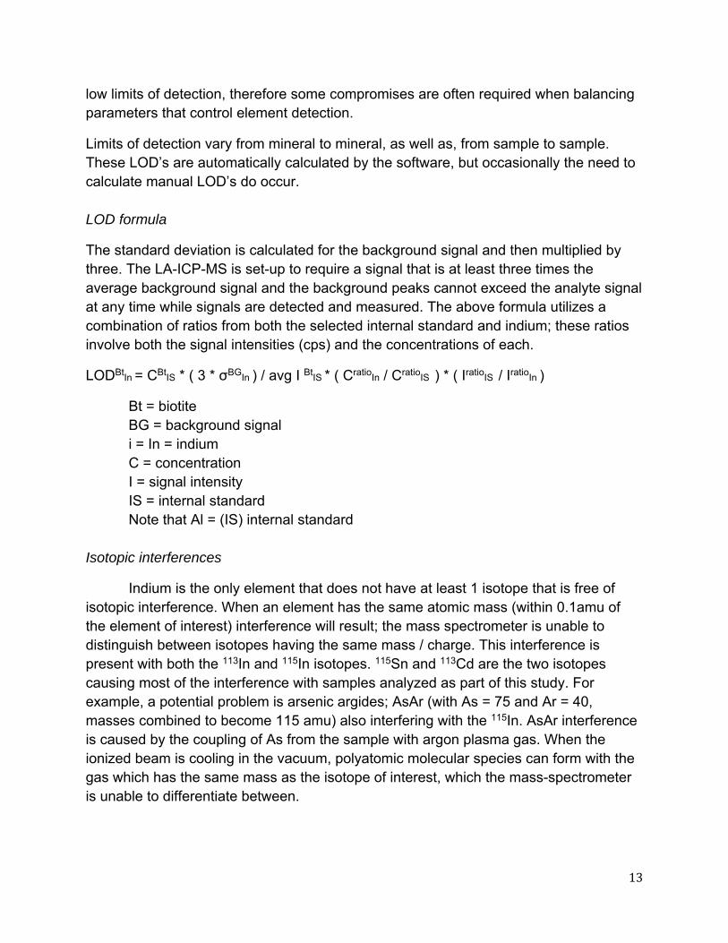
Limits of detection vary from mineral to mineral, as well as, from sample to sample. These LOD’s are automatically calculated by the software, but occasionally the need to calculate manual LOD’s do occur. LOD formula
The standard deviation is calculated for the background signal and then multiplied by three. The LA-ICP-MS is set-up to require a signal that is at least three times the average background signal and the background peaks cannot exceed the analyte signal at any time while signals are detected and measured. The above formula utilizes a combination of ratios from both the selected internal standard and indium; these ratios involve both the signal intensities (cps) and the concentrations of each.
LODBtIn
= CBtIS * ( 3 * σBG
In ) / avg I BtIS * ( Cratio
In / CratioIS ) * ( Iratio
IS / IratioIn )
Bt = biotite BG = background signal i = In = indium C = concentration I = signal intensity IS = internal standard Note that Al = (IS) internal standard
Isotopic interferences
Indium is the only element that does not have at least 1 isotope that is free of isotopic interference. When an element has the same atomic mass (within 0.1amu of the element of interest) interference will result; the mass spectrometer is unable to distinguish between isotopes having the same mass / charge. This interference is present with both the 113In and 115In isotopes. 115Sn and 113Cd are the two isotopes causing most of the interference with samples analyzed as part of this study. For example, a potential problem is arsenic argides; AsAr (with As = 75 and Ar = 40, masses combined to become 115 amu) also interfering with the 115In. AsAr interference is caused by the coupling of As from the sample with argon plasma gas. When the ionized beam is cooling in the vacuum, polyatomic molecular species can form with the gas which has the same mass as the isotope of interest, which the mass-spectrometer is unable to differentiate between.

14
Isotopic interference problems are corrected by using known ratios of naturally occurring isotope abundances associated with the interfering element. An appropriate isotopic ratio is chosen for use in the calculations to determine the portion of the interfering isotope contributing to the overall total signal measured for 113In or 115In. The indium signals are corrected and free of isotopic interference once the determined portion of interference is subtracted from the uncorrected 113In or 115In data.
Data Correction
Indium is the only element that does not have a non-interfering isotope; therefore corrections are required to remove these overlapping isobaric signal intensities since the mass spectrometer detector cannot distinguish between these isotopes with the same mass.
After completing the LA-ICP-MS analysis, indium signal intensities (expressed as ‘counts per second’) and concentrations (expressed as ppm) are corrected for isotopic interferences caused by the similar mass of 115Sn and 113Cd with that of 115In and 113In respectively. The correction equation relies on ratios constructed from the known natural abundances of the isotopes involved and allows calculations to determine and remove the interfering isotopic signal.
Isotopic abundances used in ratio correction calculations Element Isotopes 111 113 115 118 Correction Ratio
Cadmium (Cd) 12.8 12.2 1.05 Indium (In) 4.3 95.7
Tin (Sn) 0.3 24.2 .01 Table 1: Naturally occurring isotope abundances, with ratios (in red) used to correct the signal intensity interferences from tin and cadmium.
Isotopic ratios are used to calculate the portion of the measured signal which represents the interfering isotope and then this can be subtracted from the overall signal intensity producing the corrected indium measurement.
The correction calculations for 115In and 113In are as follows:
Corrected 115In = 115In (total uncorrected cps) – (Sn115/118)*( 118Sn cps)
Corrected 113In = 113In (total uncorrected cps) – (111Cd cps / Cd 113/111)
This calculation requires using ratios formed from the known natural isotopic abundances of those elements involved with the interferences. If an interfering element has many isotopes, it is often best to select isotopes for ratio calculations that provide the greatest difference. In the case of Sn, which has 10 natural isotopes, 118Sn is paired

15
with the interfering 115Sn isotope creating the ratio Sn (0.34/24.23). By evaluating the laser data and the amount of 118Sn measured (select isotopes are analyzed for ratio correction purposes) the amount of 115Sn interfering with the 115In can be inferred and then removed.
When the signal intensity (in cps) is corrected for 113In and 115In (using the preceding equations) these corrected signals are further utilized as ratio multipliers for correcting concentrations of the respective isotopes total concentration (in ppm). The resulting concentration represents the same proportion as that of the corrected signal / uncorrected signal ratio.
Corrected 115In concentration =
(corrected 115In, cps / uncorrected 115In, cps) * (uncorrected 115In, ppm)
Calculating the concentrations of indium
CBtIn = (CBt
IS Al x IBtIn / IBt
IS Al) x (CratioIn / Cratio
IS Al) x (IratioIS Al / Iratio
In)
The formula above can be used to calculate the concentrations of indium in the different minerals examined. The equation requires a known internal standard (IS) concentration that can be compared against the measured internal standard concentrations found in the minerals measured. Indium concentrations were determined by utilizing the known values of the internal standard (Al) in signal intensity and concentration ratios of indium and aluminum, along with the average aluminum content (IS) in the sampled mineral determined by the electron probe prior to the laser analysis.
ppm to mg/g conversions
The use of ppm can often be a source of confusion due to its varying meaning between the physics community and that of geology, both disciplines use ppm to represent different measurements / amounts. In geological applications ppm can mean just as implied, a single ppm would be 1 part per million parts, which is the same as 1/1,000,000=.000001 or .0001%, this can also be expressed as 1ppm = 1mg/kg or .001 mg/g. It is important to bear in mind that ppm does not give an actual weight value and is based on relative parts so it is more useful to express quantities of concentrations in weight percent instead of using ppm units. This conversion can be made after correction calculations are performed or done in unison with the correction calculations (see correction calculations for combining both in a single equation). If done after corrections, the conversion is just a simple matter of converting ppm to a percent based on 10,000

16
ppm’s = 1%, thus 1 ppm = .0001%; these conversions can be further exploited to represent the desired units of measurement.

17
Data and Results, Table 2 (see appendix for complete EPMA and LA-ICP-MS data tables)
Table 2 (above) Summarization of modal % and concentrations of indium measured among the mineralogy of each constituent of the TIS.
Std. Dev. Uncert # of trials
Avg. Indium [conc.] ppm mg/g
Quartz 18.0%
Biotite 10.6% 0.06 0.00006 0.01 0.01 3
Hornblende 10.9% 0.34 0.00034 0.05 0.04 3
Plagioclase 48.4% 0.05 0.00005 ins/d ins/d 2
Alkali Feldspar 10.6% n/d n/d n/d n/d 0
Titanite 0.4% b/d b/d ins/d ins/d 2
Magnetite 0.5% n/d n/d n/d n/d 0
Chlorite n/d n/d n/d n/d n/d 0
Apatite 0.2% n/d n/d n/d n/d 0
Std. Dev. Uncert # of trials
Avg. Indium [conc.] ppm mg/g
Biotite 3.7% 17.68 0.02 0.04 0.03 8
Hornblende 2.3% 0.25 0.00 0.01 0.01 6
Plagioclase 43.5% b/d b/d ins/d ins/d 5
Alkali Feldspar 23.4% b/d b/d ins/d ins/d 4
Titanite 0.6% 0.01 0.00 0.01 0.01 5
Magnetite 1.0% b/d b/d ins/d ins/d 2
Chlorite n/d 0.45 0.00 ins/d ins/d 1
Apatite 0.6% n/d n/d n/d n/d 0
Std. Dev. Uncert # of trials
Avg. Indium [conc.] ppm mg/g
Biotite 3.8% 0.22 0.00022 0.12 0.09 2
Hornblende 0.4% 0.72 0.00072 0.25 0.17 6
Plagioclase 47.7% b/d b/d ins/d ins/d 2
Alkali Feldspar 20.8% ins/d ins/d ins/d ins/d 3
Titanite 0.5% 0.01 0.00001 0.01 0.01 4
Magnetite 0.7% b/d b/d ins/d ins/d 3
Chlorite n/d ins/d ins/d ins/d ins/d 2
Apatite 0.2% n/d n/d n/d n/d 0
Std. Dev. Uncert # of trials
Avg. Indium [conc.] ppm mg/g
Biotite 1.5% n/d n/d n/d n/d 0
Hornblende 0.0% n/d n/d n/d n/d 0
Plagioclase 41.1% b/d b/d n/d n/d 2
Alkali Feldspar 29.0% b/d b/d n/d n/d 2
Titanite 0.1% b/d b/d n/d n/d 2
Magnetite 0.3% 0.03 0.00003 0.02 0.01 2
Chlorite n/d ins/d ins/d n/d n/d 4
Apatite b/d n/d n/d n/d n/d 0
HDG
CPG
JGP
MLG

18
The average indium concentrations in Table per mineral represent the laser ablation measurements collected and processed in this study. The indium concentrations listed in the table have all been corrected for isotopic interferences and then converted from ppm units to mgs of indium per grams of mineral.
Graphs 1. Modal % of the mineralogy of each TIS member.
The mineralogy of the four rocks evaluated from the Tuolumne Intrusive Suite was based on the modal analysis determined by the Bateman and Chappell (1979) study and the samples used in this research were collected by Dr. Piccoli from similar locations as those collected and used by Bateman and Chappell (1979) study.

19
Interpretations and conclusions
The data shows (chart to the left) that the ferromagnesian minerals did sequester indium at higher concentrations than those concentrations seen in the other minerals measured and analyzed. The averages for the other minerals measured for indium concentrations are unavailable due to most of the measurements falling below detectable limits.
Graph 2: Average indium concentrations in each of the ferromagnesian constituents present in their respective intruded member of the TIS
Despite the numerous complications with the laser analysis and measuring indium, the results do show clear indium trends among the minerals selected for this research project.
The determination not to analyze quartz was made at the commencement of the study due to anticipated problems associated with the ablation characteristics of quartz and a general knowledge quartz would not be a significant host for indium. Except for the ferromagnesian minerals, most of the measurements collected fell below detection, and those minerals that did have a sample(s) measured above the threshold of detection never exceeded the 0.05 ppm measured in a single plagioclase.
The exception to the single plagioclase measured was a single apatite sample, which measured 0.19 ppm of indium in the HDG and a measurement from a single microcline sample (from the CPG sample) measuring indium concentrations at 0.33 ppm. The microcline measurement should not be considered reliable due to the total of 9 samples measured and all were below detection (all < 0.12 ppm detection). Before corrections were made, the CPG showed each of the indium measurements above detection but after the Sn interfereces were removed only the 0.33 ppm measurement, and little or no confidence should be placed on this datum. Furthermore, it is worth noting that the Sn interferences seen in the data for the CPG unit were extremely high, in some cases several magnitudes greater than those seen with other minerals.
There is a clear increasing trend of indium concentrations with both the hornblende and the biotite with each progressive intrusion. The last and most felsic TIS member, the

20
JGP had no hornblende and all of the biotite analyzed had been altered to chlorite; likely the result of hydrothermal chloritization. The chlorite found in the HDG (1 sample) and the JGP (3) had indium concentrations similar to those of the biotite, ranging from 0.14 -0.34 ppm. As shown above there was some magnetite with indium averaging 0.00004 mg/g (0.04 ppm) in the JGP. There was additional indium detected in the magnetite (HDG with 0.02 ppm with 1 sample and the CPG also with a sample at 0.02 ppm) but each of these members also had a sample below detection.
Graph 3: Corrected indium concentrations in hornblende illustrating the increases of indium concentrations found in each of the TIS members as they become progressively more felsic.
The hornblende was the dominant indium bearing mineral examined with an overall average of 0.54 ppm (00054 mg/g) among the three members where present. The last member (CPG) containing hornblende averaging the highest indium concentrations evaluated in this research at 0.72 ppm (00072 mg/g) and the highest recorded measurement of any sample at 1.13 ppm (00113 mg/g); this is approximately 20 times more indium than the concentrations found in the upper continental crust (0.056 ppm).
Indium concentrations in hornblende increased with each successive intrusion by over twice the rate of the increases seen in the biotites. The mineral samples per TIS member range from no usable measurements to a high sample count of six measurements with the one exception being the eight measurements obtained from the HDG biotite.. Statistics of any sort should be viewed with extreme prejudice; however counting statistics of the arthimetic mean and the standard deviation are listed in the project summarization table per TIS member and per mineral where more than one measurement was above the limit of detection.

21
Much of the data had no usable measurements but can still provide information about the distribution of indium among those minerals simultaneously crystallizing out of the melt. The data showed that in each of the TIS members, indium preferentially partitioned into the ferromagnesian constituents over the other minerals examined. The indium concentrations in biotite consistently had a minimal amount of Sn interference when corrected, unlike the titanite, which upon correction fell below detection in many cases. Most of the corrections made utilized the Sn 115/118 ratio, which provided a better ratio for the calculations with a greater spread between the abundance of the two isotopes. The isotopic interference corrections on the MLG data used the 117Sn isotope for the calculation ratio, unlike all of the other corrections made, due to 118Sn not part of the initial data set received.
Graph 4: Indium concentrations before and after corrections are made to the laser analysis data. Corrections vary from mineral to mineral with the highest variations seen in the titanite. The isotopic interference for 115In were all related to the 115Sn.
Some data has been difficult to interpret or understand and may ultimately prove erroneous. A sample of chlorite measured from the CPG sample had elevated 117Sn and 118Sn levels on the order of 2-3 magnitudes greater, suggesting a potential error or contamination from ablating the glass thin section (all of this is speculative but these values warrant suspicion).

22
Graph 5: Corrected indium concentratons in the hornblende among the MLG, HDG, and the CPG. There was no hornblende present in JGP (the most felsic end member of the TIS).
Hornblende measured consistently the highest indium concentrations, with progressive increases with each subsequent intrusion; MLG averaged about 0.0001 mg indium per gram of hornblende (0.10 ppm). There was a near five times increase with indium in the HDG, averaging 0.00053 mg/g of indium in hornblende (0.53 ppm). The CPG showed even higher indium concentrations, averaging 0.00069 mg/g and the highest measured indium concentration in this study at 1.11 ppm or 0.0011 mg/g indium per hornblende.
Graphs 6 (below): Measurements of indium concentrations obtained from the mineralogy present in each of theTIS member.

23
The trends among each of the TIS members show the indium distributed within the ferromagnesian minerals at higher indium concentrations and very low to no measurements for the other major mineral constituents. The chloritization of biotite is shown in the JGP and the indium concentrations are consistent with those levels of indium found in the biotite of the other TIS members that preceded emplacement of the JGP. The chloritization of the biotite found in the JGP suggests hydrothermal alteration, which would be consistent with a more shallow and later stage magmatic emplacement. Based on the small amount of data analyzed in the research project, it can be surmised that this transition from a granodiorite to a granite, as characterized by the CPG and the JGP emplacement respectively, might be the most likely step in the evolutionary process of the silicate magma system where indium is removed by hydrothermal activity along with other ore-forming elements where potential ore deposits might form near distal margins of the magmatic system.

24
Graph 7: shows the relationship with iron and FeO + MgO showing a positive correlation that suggests that as FeO increases the MgO stays relatively constant. The increases seen with the Fe abundance in the ferromagnesian minerals appears to increase relative to each successive emplacement where fewer ferromagnesian minerals form from the melt but tend to have a greater capacity for indium concentrations. I do not have enough data to state this relationship with amount of certainty but might be an area of research that would benefit from further evaluation.
REFERENCES Bateman, P. C., & Chappell, B. W. (1979). Crystallization, fractionation, and solidification of the Tuolumne Intrusive Series, Yosemite National Park, California. Geological Society of America Bulletin, 90(5), I465-i482.
Burke, E. A. J. and Kieft, C. (1980) Canadian Mineral Coleman, D. S., & Glazner, A. F. (1997). The Sierra Crest magmatic event; rapid formation of juvenile crust during the Late Cretaceous in California. International Geology Review, 39(9), 768-787.
Coleman, D. S., Gray, W., & Glazner, A. F. (2004). Rethinking the emplacement and evolution of zoned plutons; geochronologic evidence for incremental assembly of the Tuolumne Intrusive Suite, California. Geology [Boulder], 32(5), 433-436. doi:10.1130/G20220.1
Cook, N. J., Ciobanu, C. L., Pring, A., Skinner, W., Shimizu, M., Danyushevsky, L., Saini-Eidukat, B., ... Melcher, F. (January 01, 2009). Trace and minor elements in sphalerite: A LA-ICPMS study. Geochimica Et Cosmochimica Acta, 73, 16, 4761-4791.

25
Glazner, A. F., Bartley, J. M., Coleman, D. S., Gray, W., & Taylor, R. Z. (2004). Are plutons assembled over millions of years by amalgamation from small magma chambers?. GSA Today, 14(4-5), 4-11.
Guenther, D., & Heinrich, C. (n.d.). Enhanced sensitivity in laser ablation-ICP mass spectrometry using helium-argon mixtures as aerosol carrier. Journal of Analytical Atomic Spectrometry, 1363-1368.
Guenther, D., Audetat, A., Frischknecht, R., & Heinrich, C. A. (January 01, 1998). Quantitative analysis of major, minor and trace elements in fluid inclusions using laser ablation-inductively coupled plasma mass spectrometry. Journal of Analytical Atomic Spectrometry, 13, 4, 263-270.
Hedenquist, J. W., & Lowenstern, J. B. (August 18, 1994). The role of magmas in the formation of hydrothermal ore deposits. Nature, 370, 6490, 519-527.
Hu, Z., & Gao, S. (January 01, 2008). Upper crustal abundances of trace elements: A revision and update. Chemical Geology, 253, 3, 205-221.
Kesler, S. E. (2007). Mineral supply and demand into the 21st century. U. S. Geological Survey Circular, 55-62.
Naney, M. (1983). Phase equilibria of rock-forming ferromagnesian silicates in granitic systems. American Journal of Science, 993-1033.
Paterson, S. R. (2009). Magmatic tubes, pipes, troughs, diapirs, and plumes; late-stage convective instabilities resulting in compositional diversity and permeable networks in crystal-rich magmas of the Tuolumne Batholith, Sierra Nevada, California.Geosphere, 5(6), 496-527. doi:10.1130/GES00214.1
Reid, J. r., Murray, D. P., Hermes, O., & Steig, E. J. (1993). Fractional crystallization in granites of the Sierra Nevada; how important is it?. Geology [Boulder], 21(7), 587-590. doi:10.1130/0091-7613(1993)021<0587:FCIGOT>2.3.CO;2
Relvas, J. M. R. S., Barriga, F. J. A. S., Ferreira, A., Noiva, P. C., Pacheco, N., & Barriga, G. (January 01, 2006). Hydrothermal Alteration and Mineralization in the Neves-Corvo Volcanic-Hosted Massive Sulfide Deposit, Portugal: I. Geology, Mineralogy, and Geochemistry. Economic Geology, 101, 4, 753-790.
Rudnick, R. L. (1995). Making continental crust. Nature, 378(6557), 571. Retrieved from http://search.proquest.com/docview/204461153?accountid=14696
Seifert, T., & Sandmann, D. (n.d.). Mineralogy and geochemistry of indium-bearing polymetallic vein-type deposits: Implications for host minerals from the Freiberg district, Eastern Erzgebirge, Germany. Ore Geology Reviews, 1-31.
Severs, M. J., Beard, J. S., Fedele, L., Hanchar, J. M., Mutchler, S. R., & Bodnar, R. J. (2009). Partitioning behavior of trace elements between dacitic melt and plagioclase, orthopyroxene, and clinopyroxene based on laser ablation ICPMS analysis of silicate

26
melt inclusions. Geochimica Et Cosmochimica Acta, 73(7), 2123-2141. doi:10.1016/j.gca.2009.01.009
Sinclair, W. D., Kooiman, G. J. A., Martin, D. A., & Kjarsgaard, I. M. (January 01, 2006). Geology, geochemistry and mineralogy of indium resources at Mount Pleasant, New Brunswick, Canada. Ore Geology Reviews, 28, 1, 123-145.
Solgadi, F. F., & Sawyer, E. W. (2008). Formation of igneous layering in granodiorite by gravity flow; a field, microstructure and geochemical study of the Tuolumne Intrusive Suite at Sawmill Canyon, California. Journal Of Petrology, 49(11), 2009-2042. doi:10.1093/petrology/egn056
Special Issue, 50, 192-194, Bratislava. Taylor, S. R., & McLennan, S. M. (1985). The continental crust, its composition and evolution: An examination of the geochemical record preserved in sedimentary rocks. Oxford: Blackwell Scientific.
Wager, L., Smit, J. R., & Irving, H. H. (1958). Indium content of rocks and minerals from the Skaergaard intrusion, East Greenland. Geochimica Et Cosmochimica Acta, 13(2-3), 81-86.
Wedepohl, K. H. (1969). Handbook of geochemistry. Berlin: Springer.
You, C.-F., Castillo, P. R., Gieskes, J. M., Chan, L. H., & Spivack, A. J. (January 01, 1996). Trace element behavior in hydrothermal experiments: Implications for fluid processes at shallow depths in subduction zones. Earth and Planetary Science Letters,140, 41-52.
Zellmer, G. F., & Annen, C. (2008). An introduction to magma dynamics. Geological Society Special Publications, 3041-13. doi:10.1144/SP304.1

27
Appendix
Appendix: Samples
The four thin sections yielding data are from the Tuolumne Intrusive Suite, in NE California
Y‐56 May Lake sample (granodiorite)
The scanned thin section samples shown are colored scans with dimensions of ~26 mm x 16 mm.
Y‐59 Half Dome Granodiorite

28
Y‐17 Catherdral Peak Granodiorite (thin section dimensions of ~26 mm x 16 mm)
Y‐22 Johnson Granite Porphryr

29
Appendix: EPMA Data
Standards Used
Operating Conditions
15 kV Accelerating Voltage
20 nA Cup Current
1‐20 micron beam diameter
Element Amphibole Biotite Sphene
Na Kakanui Hornblende Kakanui Hornblende Plagioclase
Fe Kakanui Hornblende Kakanui Hornblende Kakanui Hornblende
Ca Kakanui Hornblende Kakanui Hornblende Sphene
K Kakanui Hornblende Orthoclase Kakanui Hornblende
Al Kakanui Hornblende Kakanui Hornblende Kakanui Hornblende
Mg Kakanui Hornblende Kakanui Hornblende Kakanui Hornblende
Mn Rhodonite Rhodonite Rhodonite
Ti Kakanui Hornblende Kakanui Hornblende Sphene
Si Kakanui Hornblende Kakanui Hornblende Sphene
Element Feldspar Magnetite
Na Plagioclase Kakanui Hornblende
Fe Kakanui Hornblende Magnetite
Ca Plagioclase Plagioclase
K Orthoclase Kakanui Hornblende
Al Orthoclase Kakanui Hornblende
Mg Kakanui Hornblende Kakanui Hornblende
Mn Rhodonite Rhodonite
Ti Kakanui Hornblende Ilmenite
Si Orthoclase Kakanui Hornblende

30
Sample: Y‐56 May Lake Biotite
No. # Na2O FeO CaO K2O Al2O3 MgO MnO TiO2 SiO2 Total wt %
Detection Limits (ppm) 100 220 160 100 140 120 180 480 150
Region 1 1_1 0.09 19.92 b/d 9.54 15.03 11.57 0.29 4.23 37.02 97.70
1_2 0.10 19.81 b/d 9.51 14.94 11.60 0.27 4.17 36.90 97.29
1_3 0.06 19.98 b/d 9.54 15.00 11.57 0.25 4.32 37.18 97.91
1_4 0.07 20.23 b/d 9.43 14.87 11.63 0.26 4.23 36.90 97.62
1_5 0.08 19.56 b/d 9.37 14.76 11.28 0.27 4.18 36.65 96.13
1_6 0.08 20.08 b/d 9.55 14.82 11.16 0.27 4.11 37.17 97.24
1_7 0.08 20.08 b/d 9.39 14.70 11.42 0.29 4.25 36.68 96.88
1_8 0.08 20.52 b/d 9.17 14.99 11.66 0.28 4.17 36.87 97.74
1_9 0.10 20.35 b/d 9.10 15.17 11.80 0.27 4.08 36.94 97.81
1_10 0.07 20.09 b/d 9.32 14.99 11.63 0.29 4.03 37.24 97.68
1_11 0.07 20.21 b/d 9.51 14.89 11.62 0.26 4.12 37.14 97.81
1_12 0.10 20.10 b/d 9.44 14.90 11.55 0.26 4.30 36.88 97.54
1_13 0.12 20.28 b/d 9.62 14.90 11.52 0.27 4.30 37.18 98.20
1_14 0.11 20.16 b/d 9.50 14.69 11.65 0.27 4.05 36.94 97.36
1_15 0.07 20.17 b/d 9.47 14.86 11.35 0.26 4.16 36.73 97.07
1_16 0.07 20.02 b/d 9.39 15.03 11.42 0.29 4.20 37.17 97.59
1_17 0.10 20.12 b/d 9.26 14.78 11.21 0.28 4.14 36.49 96.38
1_18 0.09 20.33 b/d 9.57 14.92 11.64 0.29 3.90 37.04 97.77
1_19 0.07 20.35 b/d 9.19 15.04 11.48 0.30 4.08 37.04 97.55
1_20 0.08 20.37 b/d 9.53 15.07 11.20 0.31 3.99 37.18 97.73
Trav #2 2_1 0.10 20.24 b/d 9.18 14.98 11.20 0.28 4.05 37.25 97.28
2_2 0.07 20.64 b/d 8.84 15.21 11.43 0.30 4.01 36.76 97.25
2_3 0.10 20.29 b/d 9.24 14.81 11.38 0.26 4.09 37.08 97.25
2_4 0.09 20.13 b/d 9.12 15.01 11.44 0.30 4.12 37.02 97.22
2_5 0.09 20.03 b/d 9.12 15.07 11.40 0.33 4.09 37.13 97.26
2_6 0.12 20.22 b/d 8.80 14.99 11.48 0.31 3.96 36.90 96.77
2_8 0.13 18.80 b/d 8.41 15.50 10.69 0.25 3.75 39.56 97.08
2_9 0.10 20.24 b/d 9.00 15.25 11.33 0.30 4.03 37.33 97.57
2_10 0.11 20.05 b/d 8.95 15.19 11.04 0.29 3.98 36.78 96.38
2_11 0.10 20.10 b/d 8.83 15.23 11.27 0.26 4.12 37.11 97.03
2_12 0.09 20.15 b/d 9.21 15.06 11.46 0.33 4.17 37.32 97.79
2_14 0.07 20.05 b/d 9.00 15.24 11.45 0.36 4.14 37.45 97.76
sample cnt 2_15 0.11 19.98 b/d 8.89 15.55 11.40 0.32 3.93 38.10 98.30
33.00
Average 0.09 20.11 Ins. Data 9.24 15.01 11.42 0.29 4.10 37.12
Standard Dev 0.02 0.31 Ins. Data 0.29 0.20 0.22 0.03 0.12 0.52
31
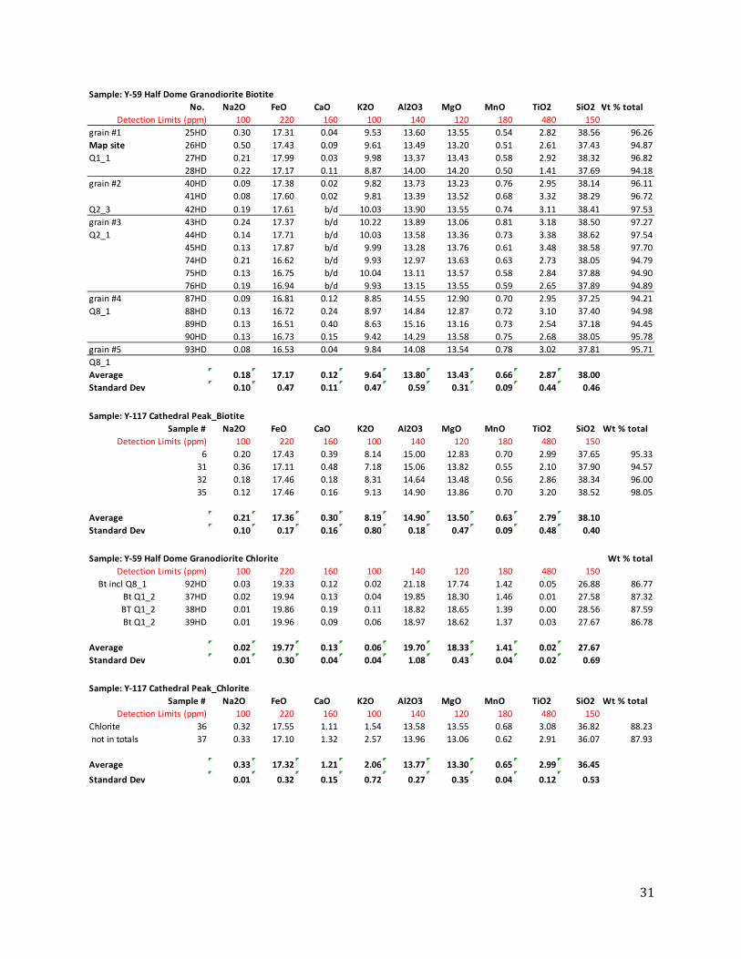
Sample: Y‐59 Half Dome Granodiorite Biotite
No. Na2O FeO CaO K2O Al2O3 MgO MnO TiO2 SiO2 Wt % total
Detection Limits (ppm) 100 220 160 100 140 120 180 480 150
grain #1 25HD 0.30 17.31 0.04 9.53 13.60 13.55 0.54 2.82 38.56 96.26
Map site 26HD 0.50 17.43 0.09 9.61 13.49 13.20 0.51 2.61 37.43 94.87
Q1_1 27HD 0.21 17.99 0.03 9.98 13.37 13.43 0.58 2.92 38.32 96.82
28HD 0.22 17.17 0.11 8.87 14.00 14.20 0.50 1.41 37.69 94.18
grain #2 40HD 0.09 17.38 0.02 9.82 13.73 13.23 0.76 2.95 38.14 96.11
41HD 0.08 17.60 0.02 9.81 13.39 13.52 0.68 3.32 38.29 96.72
Q2_3 42HD 0.19 17.61 b/d 10.03 13.90 13.55 0.74 3.11 38.41 97.53
grain #3 43HD 0.24 17.37 b/d 10.22 13.89 13.06 0.81 3.18 38.50 97.27
Q2_1 44HD 0.14 17.71 b/d 10.03 13.58 13.36 0.73 3.38 38.62 97.54
45HD 0.13 17.87 b/d 9.99 13.28 13.76 0.61 3.48 38.58 97.70
74HD 0.21 16.62 b/d 9.93 12.97 13.63 0.63 2.73 38.05 94.79
75HD 0.13 16.75 b/d 10.04 13.11 13.57 0.58 2.84 37.88 94.90
76HD 0.19 16.94 b/d 9.93 13.15 13.55 0.59 2.65 37.89 94.89
grain #4 87HD 0.09 16.81 0.12 8.85 14.55 12.90 0.70 2.95 37.25 94.21
Q8_1 88HD 0.13 16.72 0.24 8.97 14.84 12.87 0.72 3.10 37.40 94.98
89HD 0.13 16.51 0.40 8.63 15.16 13.16 0.73 2.54 37.18 94.45
90HD 0.13 16.73 0.15 9.42 14.29 13.58 0.75 2.68 38.05 95.78
grain #5 93HD 0.08 16.53 0.04 9.84 14.08 13.54 0.78 3.02 37.81 95.71
Q8_1
Average 0.18 17.17 0.12 9.64 13.80 13.43 0.66 2.87 38.00
Standard Dev 0.10 0.47 0.11 0.47 0.59 0.31 0.09 0.44 0.46
Sample: Y‐117 Cathedral Peak_Biotite
Sample # Na2O FeO CaO K2O Al2O3 MgO MnO TiO2 SiO2 Wt % total
Detection Limits (ppm) 100 220 160 100 140 120 180 480 150
6 0.20 17.43 0.39 8.14 15.00 12.83 0.70 2.99 37.65 95.33
31 0.36 17.11 0.48 7.18 15.06 13.82 0.55 2.10 37.90 94.57
32 0.18 17.46 0.18 8.31 14.64 13.48 0.56 2.86 38.34 96.00
35 0.12 17.46 0.16 9.13 14.90 13.86 0.70 3.20 38.52 98.05
Average 0.21 17.36 0.30 8.19 14.90 13.50 0.63 2.79 38.10
Standard Dev 0.10 0.17 0.16 0.80 0.18 0.47 0.09 0.48 0.40
Sample: Y‐59 Half Dome Granodiorite Chlorite Wt % total
Detection Limits (ppm) 100 220 160 100 140 120 180 480 150
Bt incl Q8_1 92HD 0.03 19.33 0.12 0.02 21.18 17.74 1.42 0.05 26.88 86.77
Bt Q1_2 37HD 0.02 19.94 0.13 0.04 19.85 18.30 1.46 0.01 27.58 87.32
BT Q1_2 38HD 0.01 19.86 0.19 0.11 18.82 18.65 1.39 0.00 28.56 87.59
Bt Q1_2 39HD 0.01 19.96 0.09 0.06 18.97 18.62 1.37 0.03 27.67 86.78
Average 0.02 19.77 0.13 0.06 19.70 18.33 1.41 0.02 27.67
Standard Dev 0.01 0.30 0.04 0.04 1.08 0.43 0.04 0.02 0.69
Sample: Y‐117 Cathedral Peak_Chlorite
Sample # Na2O FeO CaO K2O Al2O3 MgO MnO TiO2 SiO2 Wt % total
Detection Limits (ppm) 100 220 160 100 140 120 180 480 150
Chlorite 36 0.32 17.55 1.11 1.54 13.58 13.55 0.68 3.08 36.82 88.23
not in totals 37 0.33 17.10 1.32 2.57 13.96 13.06 0.62 2.91 36.07 87.93
Average 0.33 17.32 1.21 2.06 13.77 13.30 0.65 2.99 36.45
Standard Dev 0.01 0.32 0.15 0.72 0.27 0.35 0.04 0.12 0.53

32
Sample: Y‐22 Johnson Granite Porphryr_Chlorite Wt % total
Detection Limits (ppm) 100 220 160 100 140 120 180 480 150
Chlorite 41 0.21 16.17 0.85 1.44 18.05 14.79 1.09 0.05 38.02 90.66
42 0.25 14.79 1.09 1.54 17.48 13.62 0.85 0.02 38.85 88.48
43 0.21 14.37 1.06 1.69 23.21 13.44 1.03 0.04 33.96 89.02
69 0.30 9.62 1.00 1.75 37.32 8.93 0.65 0.04 28.38 87.99
Average 0.24 13.74 1.00 1.60 24.02 12.70 0.90 0.04 34.80
Standard Dev 0.04 2.85 0.11 0.14 9.24 2.58 0.20 0.01 4.79
Sample: Y‐17 Cathedral Peak_Titanite
Sample # Na2O FeO CaO K2O Al2O3 MgO MnO TiO2 SiO2 Wt % total
Detection Limits (ppm) 85 220 150 100 120 120 180 480 150
16 0.03 1.46 28.25 b/d 1.30 0.02 0.16 38.03 30.24 99.50
24 b/d 1.47 28.45 b/d 1.22 0.01 0.13 38.35 30.10 99.73
27 b/d 1.24 28.25 b/d 1.08 b/d 0.14 38.00 30.03 98.74
28 0.01 1.32 28.35 0.01 1.06 0.02 0.15 38.51 29.93 99.37
33 0.02 1.52 28.29 0.01 1.15 b/d 0.12 38.08 29.21 98.40
34 0.01 1.47 28.27 b/d 1.22 0.02 0.18 37.26 29.91 98.34
Average 0.02 1.41 28.31 0.01 1.17 0.02 0.15 38.04 29.90
Standard Dev 0.01 0.11 0.08 0.00 0.09 0.00 0.02 0.43 0.36
Sample: Y‐22 Johnson Granite Porphryr_Titanite Wt % total
Detection Limits (ppm) 85 220 150 100 120 120 180 480 150
66 0.02 1.51 27.86 b/d 1.21 0.01 0.17 38.13 30.39 99.29
67 0.04 2.10 28.28 b/d 1.68 b/d 0.35 36.73 30.39 99.58
Average 0.03 1.81 28.07 Ins. Data 1.44 0.01 0.26 37.43 30.39
Standard Dev 0.02 0.42 0.30 Ins. Data 0.33 Ins. Data 0.13 0.99 0.00
Sample: Y‐59 HDG_Titanite
Sample ID No. Na2O FeO CaO K2O Al2O3 MgO MnO TiO2 SiO2 Wt % total
Map Site Detection Lim 85 220 480 100 120 120 180 150 150
grain #1 33 b/d 1.52 29.00 b/d 1.50 0.02 0.20 36.16 32.47 100.86
Q1_2 34 b/d 1.44 28.82 b/d 1.48 b/d 0.14 36.44 32.13 100.47
35 b/d 1.17 28.56 b/d 1.34 b/d 0.14 36.69 32.06 99.97
36 b/d 1.57 28.18 b/d 1.39 b/d 0.18 35.96 31.72 99.00
grain #2 46 0.03 1.65 28.69 0.01 1.70 b/d 0.21 35.82 32.15 100.27
Q2_1 47 0.02 1.27 29.31 b/d 1.43 b/d 0.19 36.20 32.35 100.79
48 0.11 1.16 29.09 0.05 1.29 b/d 0.16 36.13 31.46 99.46
grain #3 49 b/d 1.29 28.49 b/d 1.32 0.02 0.15 35.94 31.38 98.60
Q3_1 50 b/d 1.83 27.81 b/d 1.82 0.04 0.15 34.46 31.09 97.20
51 0.01 1.42 28.44 0.02 1.59 b/d 0.13 35.96 31.61 99.19
grain #4 57 0.04 1.24 28.41 b/d 1.47 b/d 0.24 35.44 31.88 98.75
Q3_3 58 0.01 1.43 28.87 b/d 1.49 b/d 0.18 35.71 32.10 99.79
59 b/d 1.32 28.91 b/d 1.51 0.02 0.14 35.92 32.09 99.92
66 b/d 1.47 28.41 b/d 1.42 0.02 0.23 35.78 31.80 99.15
grain #5 99 b/d 1.49 28.69 b/d 1.56 b/d 0.16 35.94 31.79 99.63
Q4_3 100 0.02 1.16 28.84 b/d 1.10 b/d 0.13 36.82 31.82 99.90
101 b/d 1.26 29.19 b/d 0.91 0.01 0.15 37.05 32.20 100.77
102 0.01 1.60 28.77 b/d 1.71 0.04 0.16 35.88 31.99 100.17
Average 0.03 1.41 28.69 0.03 1.45 0.03 0.17 36.02 31.89
Standard Dev 0.03 0.19 0.37 0.02 0.21 0.01 0.03 0.56 0.35

33
Sample: Y‐59 HDG Hornblende
Sample ID No. Na2O FeO CaO K2O Al2O3 MgO MnO TiO2 SiO2 Total
Detection Lim 110 200 150 100 140 130 200 480 180
grain #1 52 0.28 12.33 13.14 0.08 1.45 16.26 0.97 b/d 55.48 100.03
Q3_2 53 1.06 13.95 12.12 0.50 5.17 14.72 0.94 0.70 50.57 99.72
54 0.53 11.65 12.52 0.16 2.65 16.43 1.04 b/d 53.87 98.89
grain #2 68 1.07 13.64 12.14 0.46 5.21 14.69 0.92 0.62 50.11 98.86
Q3_3 69 0.98 13.75 12.28 0.44 5.06 14.79 0.92 0.49 50.65 99.35
70 1.25 14.42 11.96 0.55 5.85 14.31 0.90 0.78 49.40 99.43
71 0.98 13.52 12.13 0.40 4.83 14.97 0.88 0.69 50.81 99.22
grain #3 80 1.14 13.87 11.92 0.49 4.99 14.48 0.92 0.85 49.65 98.29
Q8_1 83 0.91 13.85 12.16 0.39 4.43 14.87 1.01 0.58 50.71 98.91
Averages 0.91 13.44 12.26 0.38 4.41 15.06 0.94 0.67 51.25
Standard dev 0.29 0.83 0.35 0.15 1.34 0.71 0.05 0.11 1.92
Sample: Y‐17 Cathedral Peak_Hornblende
Sample # Na2O FeO CaO K2O Al2O3 MgO MnO TiO2 SiO2 Wt % total
Detection Limits (ppm) 110 200 150 100 140 130 200 480 180
14 1.37 15.52 11.81 0.75 7.87 12.91 0.85 1.19 44.43 96.70
15 1.32 15.15 11.63 0.68 7.23 13.26 0.83 1.11 45.40 96.61
17 1.35 14.57 11.76 0.70 7.34 13.59 0.71 1.17 47.34 98.52
23 1.43 14.69 11.70 0.75 7.76 13.00 0.73 1.28 46.70 98.03
25 1.29 14.33 11.71 0.77 7.30 13.21 0.82 1.19 46.42 97.03
26 1.35 15.28 11.95 0.75 7.57 13.17 0.92 1.14 46.61 98.74
Averages 1.35 14.92 11.76 0.73 7.51 13.19 0.81 1.18 46.15
Standard dev 0.04 0.42 0.10 0.03 0.24 0.22 0.07 0.05 0.96
Sample: Y‐59 HDG Microcline
Sample ID No. Na2O FeO CaO K2O Al2O3 MgO MnO TiO2 SiO2 Wt % total
tion Limits (ppm) 85 220 150 100 120 120 180 480 150
Map site 94 0.28 0.03 b/d 15.57 18.39 b/d b/d b/d 64.68 98.98
grain #1 95 0.41 0.08 b/d 15.41 18.30 b/d b/d b/d 65.29 99.50
Q4_3 96 0.62 0.08 b/d 15.12 18.61 b/d b/d b/d 65.34 99.79
97 0.61 0.06 b/d 14.95 18.23 0.02 0.03 0.09 65.30 99.28
98 0.56 0.09 b/d 15.23 18.43 b/d b/d 0.06 65.27 99.67
Averages 0.50 0.07 Ins. Data 15.26 18.39 0.02 0.03 0.07 65.18
Standard Dev 0.15 0.02 Ins. Data 0.24 0.14 Ins. Data Ins. Data 0.02 0.28
Sample: Y‐17 Cathedral Peak_Microcline
No. Na2O FeO CaO K2O Al2O3 MgO MnO TiO2 SiO2 Wt % total
Detection Limits (ppm) 85 220 150 100 120 120 180 480 150
11 0.67 0.08 b/d 15.90 18.42 b/d b/d b/d 64.84 99.92
19 1.15 0.07 b/d 14.97 19.17 b/d b/d b/d 64.92 100.29
20 0.97 0.07 0.03 15.16 19.29 b/d b/d b/d 65.06 100.59
21 0.85 0.09 b/d 15.61 19.08 b/d b/d b/d 64.14 99.77
Averages 0.91 0.08 0.03 15.41 18.99 Ins. Data Ins. Data Ins. Data 64.74
Standard Dev 37.61 98.35 106.05 37.83 45.17 Ins. Data Ins. Data Ins. Data 38.13
Sample: Y‐22 Johnson Granite Porphryr_Microcline
No. Na2O FeO CaO K2O Al2O3 MgO MnO TiO2 SiO2 Wt % total
85 220 150 100 120 120 180 480 150
57 0.42 0.03 0.05 16.30 20.37 b/d 0.02 b/d 64.44 101.63
Averages 0.03 0.05 16.30 20.37 Ins. Data 0.02 Ins. Data 64.44
Standard Dev Ins. Data Ins. Data Ins. Data Ins. Data Ins. Data Ins. Data Ins. Data Ins. Data Ins. Data
Detection Limits (ppm)

34
Sample: Y‐59 HDG_Magnetite
Sample ID No. Na2O FeO CaO K2O Al2O3 MgO MnO TiO2 SiO2 Wt % total
Map site Detection L 100 240 170 130 150 130 240 300 140
grain #1 29 0.41 92.73 b/d 0.09 0.17 0.03 0.15 0.16 b/d 93.79
Q1_1 30 0.36 93.79 b/d 0.05 0.17 0.04 0.24 0.22 0.03 94.91
31 0.07 94.68 b/d b/d 0.11 b/d 0.35 0.09 b/d 95.31
32 0.06 94.54 b/d 0.03 0.11 b/d 0.30 0.02 b/d 95.07
grain #2 55 0.03 92.61 b/d b/d 0.03 b/d 0.13 0.02 b/d 92.82
Q3_2 56 0.03 94.15 b/d b/d 0.05 b/d 0.17 b/d b/d 94.40
grain #3 60 0.00 92.07 b/d b/d 0.03 0.02 0.11 0.05 0.05 92.33
Q3_3 61 0.00 91.73 b/d b/d 0.39 b/d 0.04 0.03 b/d 92.20
62 0.02 92.19 b/d 0.01 0.05 b/d 0.15 0.06 b/d 92.51
63 0.03 92.22 b/d b/d 0.06 b/d 0.12 0.13 b/d 92.55
67 0.05 92.61 b/d b/d 0.03 b/d 0.09 0.10 0.03 92.90
grain #4 72 0.04 91.62 b/d b/d b/d b/d 0.21 0.03 0.03 `
Q4_1 73 0.00 91.03 b/d b/d b/d 0.02 0.23 0.03 b/d 91.33
grain #5 84 0.00 92.05 b/d b/d 0.03 b/d 0.19 0.02 b/d 92.29
Q8_1 85 0.03 92.00 b/d b/d 0.04 0.02 0.23 0.03 0.04 92.38
86 0.00 93.04 b/d b/d 0.06 b/d 0.19 0.02 b/d 93.31
Q4_3 91 0.01 94.06 b/d b/d 0.04 b/d 0.18 b/d b/d 94.32
grain #6 105 0.01 93.36 b/d b/d 0.06 b/d 0.38 0.05 0.03 93.90
Average 0.06 92.80 Ins. Data 0.05 0.09 0.03 0.19 0.07 0.03 93.31
Standard Dev 0.12 1.07 Ins. Data 0.04 0.09 0.01 0.09 0.06 0.01
Sample: Y‐17 Cathedral Peak_Magnetite
Sample # Na2O FeO CaO K2O Al2O3 MgO MnO TiO2 SiO2 Wt % total
Detection Limits (wt % 0.01 0.02 0.03 0.01 0.02 0.01 0.02 0.02 0.01
1 b/d 94.83 b/d b/d 0.12 b/d 0.22 0.04 0.04 95.26
2 0.12 93.44 b/d 0.03 0.14 0.02 0.68 0.03 0.05 94.51
3 0.03 93.38 b/d 0.01 0.11 b/d 0.34 b/d 0.02 93.90
38 0.14 90.97 b/d 0.01 0.15 b/d 0.36 b/d 0.08 91.72
39 0.03 91.69 b/d b/d 0.12 b/d 0.60 0.06 b/d 92.51
40 0.04 93.32 b/d b/d 0.06 b.d 0.23 b/d 0.02 93.68
Average 0.07 92.94 Ins. Data 0.02 0.12 0.02 0.41 0.04 0.04 93.60
Standard Dev 0.05 1.39 Ins. Data 0.01 0.03 Ins. Data 0.19 0.02 0.03
Sample: Y‐22 Johnson Granite Porphryr_Magnetite
No. Na2O FeO CaO K2O Al2O3 MgO MnO TiO2 SiO2 Wt % total
Detection L 100 240 170 130 150 130 240 300 140
50 0.10 89.47 b/d 0.08 0.77 0.04 0.14 0.07 1.18 91.85
51 b/d 89.19 b/d 0.04 0.34 0.06 0.15 b/d 0.77 90.55
52 0.06 91.66 b/d 0.04 0.49 0.04 0.15 0.02 0.62 93.10
59 0.04 90.27 b/d b/d 0.35 0.02 0.37 0.06 0.34 91.47
60 0.04 90.40 b/d b/d 0.38 0.04 0.36 0.08 0.39 91.70
61 0.02 91.58 b/d b/d 0.18 b/d 0.32 0.04 0.29 92.48
Average 0.05 90.43 Ins. Data 0.05 0.42 0.04 0.25 0.05 0.60 91.86
Standard Dev 0.03 1.03 Ins. Data 0.03 0.20 0.02 0.12 0.02 0.34
35
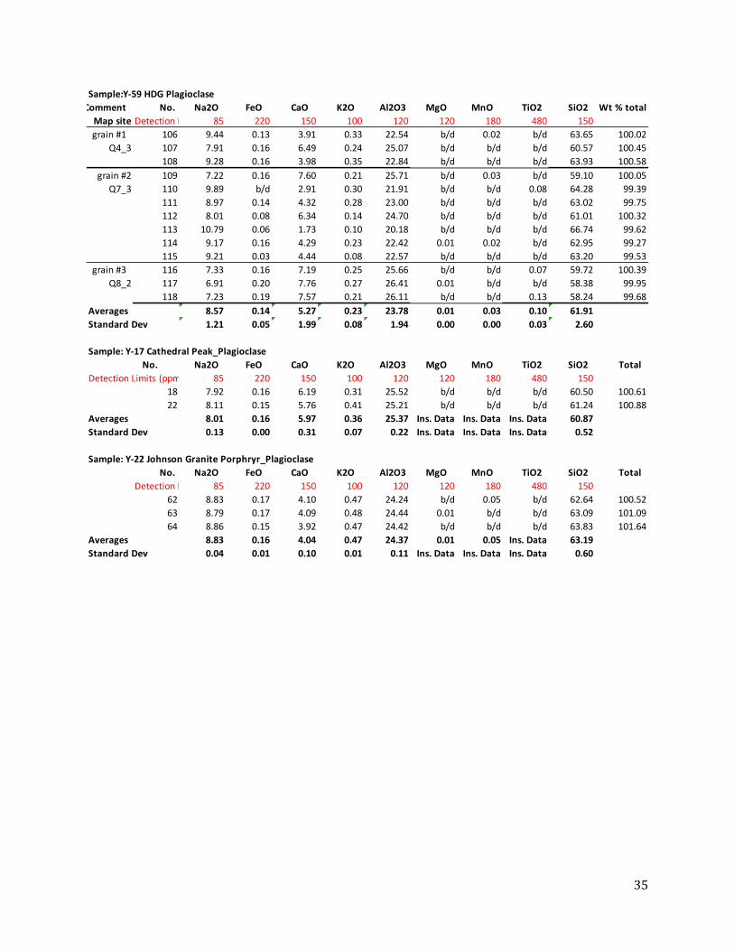
Sample:Y‐59 HDG Plagioclase
Comment No. Na2O FeO CaO K2O Al2O3 MgO MnO TiO2 SiO2 Wt % total
Map site Detection L 85 220 150 100 120 120 180 480 150
grain #1 106 9.44 0.13 3.91 0.33 22.54 b/d 0.02 b/d 63.65 100.02
Q4_3 107 7.91 0.16 6.49 0.24 25.07 b/d b/d b/d 60.57 100.45
108 9.28 0.16 3.98 0.35 22.84 b/d b/d b/d 63.93 100.58
grain #2 109 7.22 0.16 7.60 0.21 25.71 b/d 0.03 b/d 59.10 100.05
Q7_3 110 9.89 b/d 2.91 0.30 21.91 b/d b/d 0.08 64.28 99.39
111 8.97 0.14 4.32 0.28 23.00 b/d b/d b/d 63.02 99.75
112 8.01 0.08 6.34 0.14 24.70 b/d b/d b/d 61.01 100.32
113 10.79 0.06 1.73 0.10 20.18 b/d b/d b/d 66.74 99.62
114 9.17 0.16 4.29 0.23 22.42 0.01 0.02 b/d 62.95 99.27
115 9.21 0.03 4.44 0.08 22.57 b/d b/d b/d 63.20 99.53
grain #3 116 7.33 0.16 7.19 0.25 25.66 b/d b/d 0.07 59.72 100.39
Q8_2 117 6.91 0.20 7.76 0.27 26.41 0.01 b/d b/d 58.38 99.95
118 7.23 0.19 7.57 0.21 26.11 b/d b/d 0.13 58.24 99.68
Averages 8.57 0.14 5.27 0.23 23.78 0.01 0.03 0.10 61.91
Standard Dev 1.21 0.05 1.99 0.08 1.94 0.00 0.00 0.03 2.60
Sample: Y‐17 Cathedral Peak_Plagioclase
No. Na2O FeO CaO K2O Al2O3 MgO MnO TiO2 SiO2 Total
Detection Limits (ppm 85 220 150 100 120 120 180 480 150
18 7.92 0.16 6.19 0.31 25.52 b/d b/d b/d 60.50 100.61
22 8.11 0.15 5.76 0.41 25.21 b/d b/d b/d 61.24 100.88
Averages 8.01 0.16 5.97 0.36 25.37 Ins. Data Ins. Data Ins. Data 60.87
Standard Dev 0.13 0.00 0.31 0.07 0.22 Ins. Data Ins. Data Ins. Data 0.52
Sample: Y‐22 Johnson Granite Porphryr_Plagioclase
No. Na2O FeO CaO K2O Al2O3 MgO MnO TiO2 SiO2 Total
Detection L 85 220 150 100 120 120 180 480 150
62 8.83 0.17 4.10 0.47 24.24 b/d 0.05 b/d 62.64 100.52
63 8.79 0.17 4.09 0.48 24.44 0.01 b/d b/d 63.09 101.09
64 8.86 0.15 3.92 0.47 24.42 b/d b/d b/d 63.83 101.64
Averages 8.83 0.16 4.04 0.47 24.37 0.01 0.05 Ins. Data 63.19
Standard Dev 0.04 0.01 0.10 0.01 0.11 Ins. Data Ins. Data Ins. Data 0.60
36
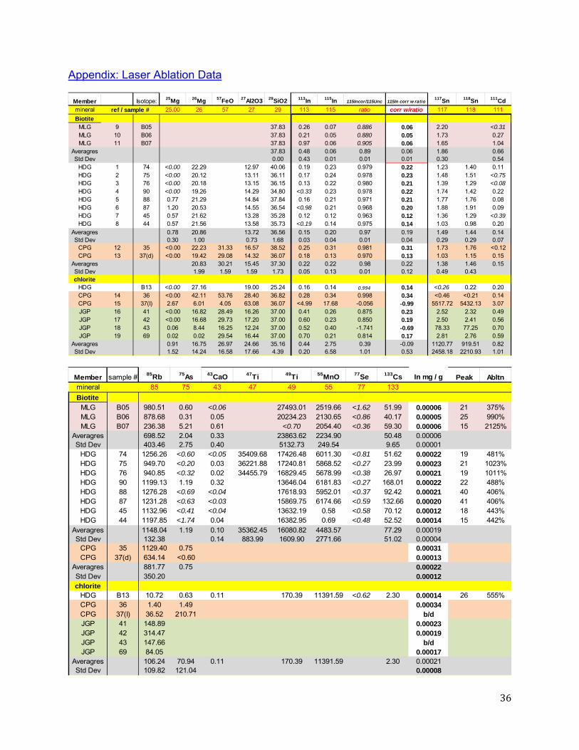
Appendix: Laser Ablation Data
Member Isotope:25Mg 26Mg 57FeO 27Al2O3 29SiO2 113In 115In 115Incor/115Unc 115In corr w ratio
117Sn 118Sn 111Cd
mineral 25.00 26 57 27 29 113 115 ratio corr w/ratio 117 118 111
BiotiteMLG 9 B05 37.83 0.26 0.07 0.886 0.06 2.20 <0.31MLG 10 B06 37.83 0.21 0.05 0.880 0.05 1.73 0.27MLG 11 B07 37.83 0.97 0.06 0.905 0.06 1.65 1.04
Averagres 37.83 0.48 0.06 0.89 0.06 1.86 0.66Std Dev 0.00 0.43 0.01 0.01 0.01 0.30 0.54
HDG 1 74 <0.00 22.29 12.97 40.06 0.19 0.23 0.979 0.22 1.23 1.40 0.11HDG 2 75 <0.00 20.12 13.11 36.11 0.17 0.24 0.978 0.23 1.48 1.51 <0.75HDG 3 76 <0.00 20.18 13.15 36.15 0.13 0.22 0.980 0.21 1.39 1.29 <0.08HDG 4 90 <0.00 19.26 14.29 34.80 <0.33 0.23 0.978 0.22 1.74 1.42 0.22HDG 5 88 0.77 21.29 14.84 37.84 0.16 0.21 0.971 0.21 1.77 1.76 0.08HDG 6 87 1.20 20.53 14.55 36.54 <0.98 0.21 0.968 0.20 1.88 1.91 0.09HDG 7 45 0.57 21.62 13.28 35.28 0.12 0.12 0.963 0.12 1.36 1.29 <0.39HDG 8 44 0.57 21.56 13.58 35.73 <0.19 0.14 0.975 0.14 1.03 0.98 0.20
Averagres 0.78 20.86 13.72 36.56 0.15 0.20 0.97 0.19 1.49 1.44 0.14Std Dev 0.30 1.00 0.73 1.68 0.03 0.04 0.01 0.04 0.29 0.29 0.07
CPG 12 35 <0.00 22.23 31.33 16.57 38.52 0.25 0.31 0.981 0.31 1.73 1.76 <0.12CPG 13 37(d) <0.00 19.42 29.08 14.32 36.07 0.18 0.13 0.970 0.13 1.03 1.15 0.15
Averagres 20.83 30.21 15.45 37.30 0.22 0.22 0.98 0.22 1.38 1.46 0.15Std Dev 1.99 1.59 1.59 1.73 0.05 0.13 0.01 0.12 0.49 0.43chlorite
HDG B13 <0.00 27.16 19.00 25.24 0.16 0.14 0.994 0.14 <0.26 0.22 0.20CPG 14 36 <0.00 42.11 53.76 28.40 36.82 0.28 0.34 0.998 0.34 <0.46 <0.21 0.14CPG 15 37(I) 2.67 6.01 4.05 63.08 36.07 <4.99 17.68 -0.056 -0.99 5517.72 5432.13 3.07JGP 16 41 <0.00 16.82 28.49 16.26 37.00 0.41 0.26 0.875 0.23 2.52 2.32 0.49JGP 17 42 <0.00 16.68 29.73 17.20 37.00 0.60 0.23 0.850 0.19 2.50 2.41 0.56JGP 18 43 0.06 8.44 16.25 12.24 37.00 0.52 0.40 -1.741 -0.69 78.33 77.25 0.70JGP 19 69 0.02 0.02 29.54 16.44 37.00 0.70 0.21 0.814 0.17 2.81 2.76 0.59
Averagres 0.91 16.75 26.97 24.66 35.16 0.44 2.75 0.39 -0.09 1120.77 919.51 0.82Std Dev 1.52 14.24 16.58 17.66 4.39 0.20 6.58 1.01 0.53 2458.18 2210.93 1.01
ref / sample #
Member sample # 85Rb 75As 43CaO 47Ti 49Ti 55MnO 77Se 133Cs In mg / g Peak Abltnmineral 85 75 43 47 49 55 77 133
BiotiteMLG B05 980.51 0.60 <0.06 27493.01 2519.66 <1.62 51.99 0.00006 21 375%MLG B06 878.68 0.31 0.05 20234.23 2130.65 <0.86 40.17 0.00005 25 990%MLG B07 236.38 5.21 0.61 <0.70 2054.40 <0.36 59.30 0.00006 15 2125%
Averagres 698.52 2.04 0.33 23863.62 2234.90 50.48 0.00006Std Dev 403.46 2.75 0.40 5132.73 249.54 9.65 0.00001
HDG 74 1256.26 <0.60 <0.05 35409.68 17426.48 6011.30 <0.81 51.62 0.00022 19 481%HDG 75 949.70 <0.20 0.03 36221.88 17240.81 5868.52 <0.27 23.99 0.00023 21 1023%HDG 76 940.85 <0.32 0.02 34455.79 16829.45 5678.99 <0.38 26.97 0.00021 19 1011%HDG 90 1199.13 1.19 0.32 13646.04 6181.83 <0.27 168.01 0.00022 22 488%HDG 88 1276.28 <0.69 <0.04 17618.93 5952.01 <0.37 92.42 0.00021 40 406%HDG 87 1231.28 <0.63 <0.03 15869.75 6174.66 <0.59 132.66 0.00020 41 406%HDG 45 1132.96 <0.41 <0.04 13632.19 0.58 <0.58 70.12 0.00012 18 443%HDG 44 1197.85 <1.74 0.04 16382.95 0.69 <0.48 52.52 0.00014 15 442%
Averagres 1148.04 1.19 0.10 35362.45 16080.82 4483.57 77.29 0.00019Std Dev 132.38 0.14 883.99 1609.90 2771.66 51.02 0.00004
CPG 35 1129.40 0.75 0.00031CPG 37(d) 634.14 <0.60 0.00013
Averagres 881.77 0.75 0.00022Std Dev 350.20 0.00012chlorite
HDG B13 10.72 0.63 0.11 170.39 11391.59 <0.62 2.30 0.00014 26 555%CPG 36 1.40 1.49 0.00034CPG 37(I) 36.52 210.71 b/dJGP 41 148.89 0.00023JGP 42 314.47 0.00019JGP 43 147.66 b/dJGP 69 84.05 0.00017
Averagres 106.24 70.94 0.11 170.39 11391.59 2.30 0.00021Std Dev 109.82 121.04 0.00008

37
Member Sample # 25Mg 26Mg 57FeO 27Al2O3 29SiO2 113In 115In 115Incor/115Unc 115In corr w ratio117Sn 118Sn 111Cd
TitaniteHDG 100 0.08 <0.07 1.29 33.46 0.60 0.33 0.002 0.00 94.98 95.47 0.84HDG 102 0.08 <0.08 1.31 32.53 0.43 0.31 -0.013 0.00 93.14 92.12 0.88HDG 46 0.17 <0.27 1.70 47.65 <0.60 0.82 0.031 0.03 238.57 233.03 <6.11HDG 48 0.34 0.45 1.29 29.12 0.56 0.36 -0.012 0.00 110.73 106.46 0.68HDG 50 0.09 <0.09 1.82 36.76 0.76 0.45 0.037 0.02 125.70 127.55 0.76
Averagres 0.15 0.45 1.48 35.91 0.59 0.45 0.01 0.01 520.22 477.59 0.84Std Dev 0.11 0.26 7.11 0.14 0.21 0.02 0.01 950.96 850.78 0.13
MLG B11 30.49 0.54 0.67 -0.048 b/d 195.36 0.73MLG B12 30.49 0.60 0.65 -0.018 b/d 185.01 0.70CPG 16 0.05 <0.05 2.14 1.18 30.24 0.37 0.30 0.049 0.01 85.69 83.42 0.48CPG 27 0.05 <0.02 2.28 1.26 30.03 0.64 0.23 0.005 0.00 67.23 68.05 0.52CPG 13 0.05 0.02 2.16 1.24 27.77 0.68 0.24 0.057 0.01 66.78 67.15 0.75CPG 18 0.06 <0.03 2.75 2.55 30.00 0.25 0.42 0.062 0.03 112.12 114.58 0.32
Averagres 0.05 0.02 2.33 1.56 29.51 0.48 0.30 0.04 0.01 82.96 83.30 0.52Std Dev 0.01 0.28 0.66 1.16 0.21 0.08 0.03 0.01 21.35 22.15 0.18
JPG 53 <0.00 18.51 3.82 1.81 26.44 0.52 0.98 -2.907 b/d 262.58 272.92 0.68JPG 66 0.05 <0.09 3.02 1.63 30.39 0.41 0.70 -3.165 b/d 208.58 207.29 0.77
Averagres 0.10 3.89 2.35 1.40 28.77 0.48 0.44 -0.34 201.29 193.46 0.61Std Dev 0.08 8.18 1.01 0.52 10.49 0.17 0.24 1.02 224.98 214.50 0.23
Member sample # 85Rb 75As 43CaO 47Ti 49Ti 55MnO 77Se 133Cs In mg / g Peak Abltn
TitaniteHDG 100 1.06 134.34 28.84 498636.80 <4.89 1222.68 124.31 0.05 0.00000 40 395%HDG 102 0.84 119.27 28.77 492136.22 <8.00 1202.29 110.52 <0.05 0.00000 36 387%HDG 46 <0.91 47.81 41.40 <18.98 0.30 21.38 <0.18 0.00003 29 138%HDG 48 29.45 17.14 25.94 <14.92 0.17 1.52 1.93 0.00000 28 223%HDG 50 2.59 382.87 32.24 <6.00 0.18 459.81 <0.05 0.00002 34 385%
Averagres 0.00002Std Dev 0.00003
MLG B11 1.91 171.31 28.91 <3.11 1034.14 199.13 <0.06 b/d 35 330%MLG B12 1.84 151.47 28.64 <16.46 1016.09 177.76 <0.05 b/d 40 306%CPG 16 0.55 85.58 0.00001CPG 27 0.65 71.29 0.00000CPG 13 0.68 68.60 0.00001CPG 18 0.80 94.64 0.00003
Averagres 0.00001Std Dev 0.00001
JPG 53 2.22 b/dJPG 66 0.79 b/d
Averagres 3.62 122.21 30.68 495386.51 639.41 156.35 0.99 0.00001Std Dev 8.17 97.73 5.07 4596.60 602.83 152.58 1.33 0.00001
Member Sample # 25Mg 26Mg 57FeO 27Al2O3 29SiO2 113In 115In 115Incor/115Unc 115In corr w ratio117Sn 118Sn 111Cd
MagnetiteHDG 55 0.11 0.28 0.05 <0.49 <0.23 0.02 0.960 0.02 <0.16 <0.27 0.20HDG 56 0.04 <0.29 0.05 <1.66 <0.36 <0.07 0.965 b/d <0.57 <0.79 <0.93CPG 1 0.01 <0.03 94.83 0.04 <0.32 <0.22 <0.01 0.788 b/d <0.84 <0.27 <0.13CPG 9 0.01 <0.02 91.96 0.41 3.55 <0.13 0.02 0.965 0.02 0.26 0.25 0.26CPG 38 0.00 <0.02 90.97 0.08 <0.13 0.03 <0.01 0.902 b/d <0.23 0.12 0.01JGP 50 0.05 0.07 89.47 0.17 0.48 0.10 0.03 0.922 0.03 <0.27 0.17 0.09JGP 51 <0.00 <0.06 89.19 0.40 1.20 0.08 0.06 0.960 0.06 <0.20 0.17 0.12
ragres (JGP only) 0.04 0.17 91.28 0.17 1.75 0.07 0.03 0.92 0.04 0.26 0.18 0.13Std Dev (JGP) 0.04 0.15 2.28 0.16 1.61 0.03 0.02 0.06 0.02 0.05 0.10
Member sample # 85Rb 75As 43CaO 47Ti 49Ti 55MnO 77Se 133Cs In mg / g Peak Abltn
MagnetiteHDG 55 <0.19 <0.42 0.09 40.57 0.13 <0.29 <0.04 0.00002 13 538%HDG 56 <0.91 <2.22 <0.10 <20.96 0.17 <3.16 <0.14 b/d 12 160%CPG 1 <0.16 <0.50 b/dCPG 9 0.13 0.44 0.00002CPG 38 <0.13 <0.28 b/dJGP 50 0.72 0.00003JGP 51 2.34 0.00006
1.06 0.44 0.09 40.57 0.15 0.000041.14 0.03 0.00002

38
Member Sample # 25Mg 26Mg 57FeO 27Al2O3 29SiO2 113In 115In 115Incor/115Unc 115In corr w ratio117Sn 118Sn 111Cd
Hornblende HHDG 52 0.39 13 1.5 28 0.58 0.38 0.995 0.38 0.69 0.55 0.68HDG 53 0.60 24 5.2 50 0.94 0.72 0.979 0.71 4.8 4.4 0.79HDG 79 0.56 20.36 4.67 45.53 0.88 0.60 0.972 0.59 4.70 4.82 0.76HDG 80 1.08 17.86 4.99 41.59 0.70 0.55 0.975 0.54 4.02 3.92 <0.68HDG 83 0.33 17.57 4.43 40.74 0.70 0.58 0.977 0.57 4.19 3.80 0.60HDG B14 0.42 20.46 5.00 44.32 <1.02 0.64 0.975 0.63 4.45 4.58 0.74
Averagres 0.57 18.89 4.29 41.72 0.76 0.58 0.98 0.57 3.80 3.69 0.72Std Dev 0.27 3.74 1.41 7.44 0.15 0.11 0.01 0.11 1.55 1.59 0.07
MLG B08 46.49 0.54 0.34 0.950 0.32 4.69 <0.09 0.39MLG B09 46.49 0.95 0.42 0.941 0.40 6.91 <0.04 0.65MLG B10 46.49 0.68 0.32 0.929 0.30 6.33 8.17 0.44
Averagres 46.49 0.72 0.36 0.94 0.34 5.98 8.17 0.49Std Dev 0.00 0.21 0.05 0.01 0.05 1.15 0.14
CPG 14 <0.00 16.60 20.77 5.64 44.43 1.04 0.66 0.980 0.65 4.08 3.91 0.35CPG 26 <0.00 18.59 24.28 7.24 46.61 0.87 0.92 0.985 0.91 3.80 3.94 0.59CPG 15 <0.00 18.53 23.08 6.42 45.40 0.85 0.60 0.980 0.59 3.92 3.53 0.64CPG 25 <0.00 18.45 22.66 7.46 46.42 0.55 0.60 0.977 0.58 3.64 4.08 0.54CPG 17 <0.00 20.61 19.78 3.90 47.34 1.01 1.14 0.994 1.13 1.92 2.11 0.77CPG 23 <0.00 19.75 23.26 6.57 46.70 0.61 0.49 0.974 0.48 4.06 3.67 0.53
Averagres 18.76 22.31 6.21 46.15 0.82 0.74 0.98 0.72 3.57 3.54 0.57Std Dev 1.36 1.69 1.30 1.05 0.20 0.25 0.01 0.25 0.83 0.73 0.14
MicroclineHDG 94 <0.01 <0.17 18.39 131.41 <0.63 <0.05 0.946 b/d <1.13 <0.51 0.35HDG 96 <0.01 <0.15 18.61 120.52 <0.68 <0.02 0.585 b/d <0.51 0.44 0.00HDG 98 <0.02 0.31 18.43 131.00 <0.56 <0.08 0.674 b/d <3.16 0.90 0.12HDG 97 <0.02 <0.29 18.23 133.97 <0.30 <0.12 1.076 b/d <1.58 <0.82 0.18JGP a12 <0.00 <0.06 <0.29 12.61 64.44 <0.27 <0.04 b/d <1.19 0.58 <0.25JGP a13 0.08 0.06 <0.30 15.04 64.44 <0.32 <0.03 b/d <0.76 <0.63 <0.36CPG 11.1 <0.12 <2.21 <8.62 0.65 64.84 <7.75 30.90 -0.062 b/d 9536.78 9611.68 <18.31CPG 11.2 0.14 0.21 <0.89 42.48 64.84 0.62 3.12 0.105 0.33 884.38 817.42 0.52CPG 11.3 0.13 <0.40 <1.71 25.86 64.84 <0.96 5.92 -0.095 b/d 1906.74 1897.98 0.55
Averagres 0.12 0.19 18.92 93.37 0.62 13.31 4109.30 2054.83 0.29Std Dev 0.03 0.12 11.14 34.21 15.30 4728.05 3776.79 0.22
Member sample #85Rb 75As 43CaO 47Ti 49Ti 55MnO 77Se 133Cs In mg / g Peak Abltn
HornblendeHDG 52 4.4 0.39 6.1 258 0.55 <0.27 0.78 0.00038 26 846%HDG 53 5.1 1.4 11 3308 0.92 0.84 0.51 0.00071 32 445%HDG 79 3.01 0.93 10.37 3287.48 6756.62 0.92 <0.05 0.00059 46 474%HDG 80 2.03 1.88 9.64 4019.40 6443.60 2.45 <0.05 0.00054 42 487%HDG 83 2.16 0.94 9.41 3067.93 6114.02 0.68 <0.04 0.00057 37 511%HDG B14 2.32 1.14 10.13 3772.36 6883.03 1.48 <0.13 0.00063 31 460%
Averagres 3.16 1.12 9.44 2952.12 4366.46 1.27 0.65 0.00057Std Dev 1.28 0.51 1.73 1365.62 3392.16 0.73 0.19 0.00011
MLG B08 3.51 1.27 10.62 7287.97 3063.72 <1.64 0.31 0.00032 40 363%MLG B09 2.76 6.69 11.63 7204.41 3780.88 10.78 0.69 0.00040 31 917%MLG B10 18.90 18.58 12.11 6531.11 4020.45 8.29 0.27 0.00030 13 883%
Averagres 8.39 8.85 11.45 7007.83 3621.68 9.54 0.42 0.00034Std Dev 9.11 8.85 0.76 414.96 497.83 1.76 0.23 0.00005
CPG 14 2.99 1.31 0.00065CPG 26 4.80 2.48 0.00091CPG 15 2.89 1.16 0.00059CPG 25 80.15 <1.14 0.00058CPG 17 1.22 0.62 0.00113CPG 23 2.15 1.41 0.00048
Averagres 15.70 1.40 0.00072Std Dev 31.60 0.68 0.00025
MicroclineHDG 94 975.16 4.93 0.39 <964.95 50.00 <71.89 <2.24 25.38 b/d 11 215%HDG 96 940.90 8.18 0.40 <748.35 44.10 <62.08 <1.46 23.09 b/d 10 259%HDG 98 1094.03 5.41 0.40 <1241.32 45.85 <104.30 <1.80 22.99 b/d 6 180%HDG 97 981.96 4.86 0.32 <1216.97 <31.57 <99.57 <1.72 26.55 b/d 10 162%JGP a12 560.95 b/dJGP a13 606.04 b/dCPG 11.1 18.24 <40.05 b/dCPG 11.2 777.29 <4.92 0.00033CPG 11.3 710.16 <11.77 b/d
Averagres 740.52 5.84 0.38 46.65 24.50 b/dStd Dev 326.49 1.58 0.04 3.03 1.76 b/d

39
Member Sample # 25Mg 26Mg 57FeO 27Al2O3 29SiO2 113In 115In 115Incor/115Unc 115In corr w ratio117Sn 118Sn 111Cd
PlagioclaseHDG 106 <0.01 <0.20 22.54 84.52 <0.28 <0.05 0.895 b/d <2.27 <0.53 0.22HDG 108 <0.02 <0.23 22.84 96.66 <0.54 <0.05 b/d b/d <2.05 <0.73 <0.58HDG 113 <0.03 <0.43 20.18 110.95 <0.54 <0.05 1.487 b/d <2.23 <1.54 0.00HDG 114 <0.01 <0.20 22.42 82.38 <0.39 <0.04 0.845 b/d <0.87 <0.48 0.23HDG 115 0.11 <0.16 22.57 84.57 0.15 <0.04 0.779 b/d <0.93 0.97 <2.10MLG B13 60.00 0.61 <0.09 2.727 b/d <0.56 <0.11 0.69MLG B14 60.00 0.65 0.06 0.911 0.05 1.42 0.26 0.68CPG 18 <0.19 <3.59 <16.30 <0.82 60.50 <8.68 52.43 -0.030 b/d 15894.36 15830.15 <32.49CPG 21 <0.00 <0.05 <0.24 16.63 64.14 <0.29 0.47 -0.054 b/d 148.81 146.77 <0.20JGP 62 <0.00 <0.05 <0.28 18.00 62.64 0.28 <0.04 b/d <1.42 <0.70 0.37JGP 63 0.01 <0.05 <0.26 17.59 63.09 0.23 <0.02 b/d <1.41 <0.47 0.24
Averagres 0.06 20.35 75.41 0.38 17.65 5348.19 3994.54 0.35Std Dev 0.07 2.60 17.52 0.23 30.12 9133.55 7890.71 0.25Apatite
HDG 119 <0.02 <0.29 0.07 <1.86 <4.91 <0.09 0.712 b/d <2.53 <0.74 <0.67HDG 120 2.11 2.84 23.57 105.25 5.57 0.52 0.362 0.19 94.75 96.59 10.70
Averagres 2.11 2.84 11.82 105.25 5.57 0.52 0.54 0.19 94.75 96.59 10.70Std Dev 16.62 0.25
Member sample # 85Rb 75As 43CaO 47Ti 49Ti 55MnO 77Se 133Cs In mg / g Peak AbltnPlagioclase
HDG 106 1.26 <2.28 4.53 <1023.78 <18.53 <71.53 <1.97 <0.09 b/d 29 156%HDG 108 0.92 <3.16 3.75 <1105.41 21.87 <80.67 <1.45 <0.12 b/d 27 141%HDG 113 14.74 <3.80 1.49 <39.57 <0.02 <1.22 0.97 b/d 7 125%HDG 114 0.72 <1.32 4.14 26.92 <0.01 <0.78 <0.09 b/d 38 180%HDG 115 18.19 <1.63 3.94 23.44 <0.01 <2.52 6.03 b/d 21 238%MLG B13 <0.43 <1.08 8.63 77.15 <23.35 <2.18 0.00 b/d 21 308%MLG B14 21.20 707.66 4.38 99.10 10.44 <0.19 0.34 0.00005 15 3723%CPG 18 <24.16 <125.02 b/dCPG 21 371.55 2.31 b/dJGP 62 1.78 b/dJGP 63 0.86 b/d
Averagres 47.91 354.99 4.41 49.69 10.44 1.84Std Dev 121.65 498.76 2.12 35.98 2.82Apatite
HDG 119 <1.03 34.56 55.37 <28.44 996.57 17.37 0.34 b/d 34 108%HDG 120 509.56 168.01 55.35 397876.36 8922.87 15.61 202.46 0.00019 10 18%
Averagres 509.56 101.29 55.36 397876.36 4959.72 16.49 101.40 b/dStd Dev 94.36 0.01 5604.74 1.25 142.92 b/d

40
Appendix: Literature Review
Bateman and Chappell (1979)
The series of intrusive events that amalgamated to form the Sierra Nevada Batholith were emplaced between 120-80 Ma during the Cretaceous period with each magmatic pulse lasting 10-15 myr. The Tuolumne Intrusive Series was emplaced in the early Late Cretaceous, making it the youngest suite of granitoids in the region (Evernden and Kistler, 1970). Alteration zones are typically characterized by hydrothermal activity were not observed, suggesting that the TIS emplacement occurred below the zone of meteoric water (Bateman and Eaton, 1967).
Crystal fractionation provides a plausible explanation for the compositional zonation observed in the TIS. The 2 possible mechanisms capable of explaining related features observed are; preferential marginal accretion coupled with inward displacement of the melt phase and downward crystal settling out of the melt and likely, simultaneous upward movement of the melt and volatile phases.
Progressive changes in fabric, textures, and mineralogy from the margins inward are evident with each of the intrusive events forming the TIS. Mafic minerals dominate the plutonic margins and decrease inward with an inverse relationship existing with the precipitation of quartz and K-spar, both of which lead to a more felsic composition as the magma proceeds to evolve. Marginal contacts also exhibit foliated textures that are parallel to the intrusions external contacts, interpreted as partly crystallized material that had stretched during emplacement and solidification processes.
Textural characteristics of the first intrusion (MLG, aka Kuna Crest) are dominated by finer grains: primarily consisting of plagioclase, biotite, and hornblende and most are anhedral with some apatite and magnetite being the exception with some equant / prismatic crystals present. As the magma evolves and additional emplacements ensue, the size and euhedral crystals from most of these minerals increase inward in the sequence. Biotite, hornblende, and sphene reach a maximum size in the middle half of the equigranular facies of the HDG. The HDG porphyritic facies, and continuing farther inward, is characterized by a decrease in the size of these mafic minerals as their abundances are reduced. Alkali feldspar grain sizes increase to the HDG equigranular / porphyry boundary where the megacrysts appear and increase in abundance up to the HDG / CP boundary, reaching their largest size (up to 6-8cm) just inside the margins of the Cathedral Peak, then the megacrysts decrease in size and abundance inward.
The last, most centralized emplacement is the Johnson Granite Porphyry, which exhibits distinct traits from the other members of the TIS: extremely fine-grained matrix, porphyritic texture, miarolitic cavities, along with angular mineral fragments all provide

41
observable evidence to the probable volcanic eruption that was coupled with the pressure quench of the Johnson Granite Porphyry formation. It has been postulated by Bunham (1972) that decompression resulted from an oversaturation of water, causing a separate aqueous phase to form and exceeded the capacity of the wall and roof rock to accommodate the additional volume and pressure increases. This scenario supports the unlikelihood that the JGP represents an end-stage melt composition and provides a reasonable explanation regarding the depletion of plagioclase and mafic minerals.
Indium distribution in a layered series of intrusions (Wager et. al, 1958)
Wager evaluated the indium distribution of a fractionated basic magma by conducting studies on the Skaergaard intrusion and assigning the composition of the chilled marginal gabbro to represent the composition of the original magma, thus producing average indium content as 0.058 ppm. Spectrographic determinations conducted by Shaw (1952) obtained an indium concentration range from 0.02 – 0.078 ppm for the 6 gabbros and dolorites and a range of 0.12 – 0.32 ppm for the 4 basalts evaluated. The standard for diabase W1, with indium concentrations at 0.064 ppm (Smales et al., 1957), is close to the values Wager noted in his study.
Wager had noted a layered series of intrusions with each progressively emplace intrusion containing higher levels of indium, ranging from 0.060 to 0.18 ppm. The hypersthene olivine gabbro (a pyroxene) was the first mineral evaluated by Wager to crystallize out of the melt and had the lowest indium content. Although ‘hypersthene’ is no longer a credited term, it has been commonly used to refer to the intermediate Fe-rich mineral; enstatite (Mg endmember) and ferrosilite (Fe endmember) are the endmembers in this solid solution series (Mg,Fe)2Si2O6. The lastest two layered rocks (the two youngest) were both iron-rich fayalite ferrogabbros which contained over double the indium content of the iron-rich enstatite, with indium present at ~ 0.15 ppm for each of these. It was observed that the biggest difference between these two layers were their relative FeS content. The last formed layer (#4328 Ferrogabbro) had a significantly higher S content at ~ 5000 ppm while the previously emplaced layer contained only ~50 ppm of Sulfur. Given what is known about the chalcophilic properties of indium, it would be intuitive to expect preferential incorporation of indium into the more sulfide-rich rock layer. Indium’s preferential affinity towards the sulfide-rich layer was not observed suggesting an immiscible sulfide liquid phase in equilibrium with the silicate magma containing elevated indium concentrations had not materialized in this case.
The acid granophyre (microgranite w/ 75% SiO2) formed from the last liquid fraction of the gabbro-like magma with an indium content of 0.091, a decrease from the latest gabbros but still higher than that of a standard (G1) granite at 0.026 ppm.

42
A late-stage basic magma was used to demonstrate the distribution of indium among the (primary five) simultaneously precipitated minerals of the hortonolite ferrogabbro (#5181) using the analysis obtained in Wagers’ study. Plagioclase is clearly an incompatible mineral phase for indium partitioning given the significantly scant indium content of ~ 0.0032 ppm. Olivine almost doubles the indium content of plagioclase, measuring 0.056 ppm; this 0.056 ppm concentration is coincidently the same ppm abundance within the upper continental crust abundance for indium as determined by Rudnick and Gao (2004). Pyroxene incorporates about 0.18 ppm indium, over double the amount of indium incorporated into the Olivine structure. The ferrous iron is primarily responsible for the indium substitutions with more readily exchanges in the augite than the olivine structure (Wager and Mitchell, 1951). Magnetite had very close indium concentrations as the augite at 0.16 ppm and ilmenite contain nearly twice that amount with 0.29 ppm, by far the most dominant indium acceptor.
Analysis was done on three early forming pyroxenes that had crystallized during different stages of fractionation. Progressing from the earliest to the latest pyroxenes to form, increases of indium correlated with the crystallizing sequence produced indium abundances of 0.17, 0.18 (Ca35Mg33Fe32), and one of the latest pyroxenes (Ca43Mg4Fe53 close to a hedenbergite) measured 1.1 ppm. This analysis demonstrates that higher indium concentrations associated with the iron-rich /lower temp pyroxenes can be attributed to a more fractionated melt in which these pyroxenes would crystallize out of sequentially. If ionic size and valency were the primary controlling substitution factors, it would be expected to find indium incorporating into the earlier forming ferromagnesian minerals more readily than the later stage, this however is clearly not the case, as demonstrated with the analyses of the three pyroxenes. It appears that in the ferromagnesian minerals the trivalent indium tends to replace the ferrous iron (divalent) despite the charge difference and the lack of similar radii (In=0.92A, Fe2+=0.83A).
The study by Wager made some important conclusions regarding indium distribution among granitic rocks found in the Skaergaard intrusion. It seems obvious from the data that the earliest forming rock to solidify from the ferrogabbro magma contained less indium than the magma from which the rock precipitated out. With each sequential mineral to crystallize out of the mix a higher indium content was observed in each of the solid phases formed, indicating an increasingly indium-enriched melt. We can assume the highest melt indium concentrations in the melt occurred at the onset with the crystallization of the granophyre. The granophyre formation clearly incorporated much of the remaining indium in the liquid. Wager concluded that indium does not become enriched in the residual liquids, basing this assessment on indium’s preferential incorporation into the ferromagnesian minerals of basic rocks, and as a direct result,

43
provides the rationale as to why granites and the mineral veins of granitic origin contain relatively low indium concentrations.
The mineralogy and chemistry of indium in sulfide deposits and implications for mineral processing (Cook et al., 2011)
Sphalerite is the most important In-bearing mineral. Very few minerals exist with indium as a major constituent and they never occur at appreciable quantities to be considered economically important. Roquesite (CuInS2) has been observed in minor amounts in association with some indium-bearing zinc ores and is only (relatively) abundant when the Zn content of the ore is very low and Cu content is high. None of the other indium-minerals (laforetite (AgInS2, sakuraiite (Cu,Zn,Fe,In,Sn)4S4, petrukite (Cu,Fe,Zn)2(Sn,In)S4, indite (FeIn2S4) or any secondary minerals provide any value beyond mineralogical / geochemical interests.
Indium occurs directly within the crystal lattice of sphalerite and can exceed concentrations of 1 wt % (10,000 ppm or 10 mg indium per 1 g sphalerite), as observed at Mount Pleasant, New Brunswick, Canada or the Erzgebirge provenance in Germany. The Toyoha deposit in Japan is a significant indium producer prior to its closer in 2005. More commonly, indium is found in sphalerite ranging from a few ppm to a few hundreds of ppm, very rarely exceeding 1000 ppm. These commonly low concentration levels of indium require the mining of indium as a by-product in conjunction with Zn-ore extraction processes.
(Cook et al., 2009) used LA-ICP-MS to demonstrate lattice bound indium had varying concentrations (across several orders of magnitude: <1 ppm to >5 wt. %). In each of these cases, indium was incorporated into the sphalerite structure by simple coupled substitution of; 2 Zn2+ Cu+ + In3+. These LA studies also provided evidence that depth profiles are always flat for indium indicating a homogenous distribution of indium within the sphalerite lattice.
The other mineral that is often an indium-carrier (although at lower levels than sphalerite) includes chalcopyrite (Gaspar, 2002). When both these minerals are present, sphalerite out competes chalcopyrite for the incorporation of indium into its mineral structure. Only when sphalerite content is low can chalcopyrite contain relatively significant amounts of indium. Some other minerals likely to contain some indium (although rarely at levels to make them viable / potential ores) include stannite, ferrokesterite and stannoidite (Schwarz-Schampera and Herzig, 2002; Jovic et al., 2011).
Granite related ore-deposits have received more research focus than other deposit types over the last few decades. With the diversity of ore-deposit classes and types, styles of mineralization and formation processes, it is likely these factors have

44
contributed to the few papers that encompass the ore-forming processes as a single investigation that models enrichment processes of ore-forming elements (OFE’s).
The parameters which influence potential exploratory targets for a given metallic resource are still not well understood and our present understanding of granite-related mineralization and ore-bearing deposits continues to be enhanced with ongoing studies. Some of these ongoing studies and areas of knowledge deficiency are: Wang et al. (2011) studing skarn systems and their distribution / migration patterns of An, Ag, Cu, Pb, and Zn during the ore forming processes near Tongling, China where skarn type ore- fields formed around several magmatic plutons.
Phase equilibria of rock-forming ferromagnesian silicates in granitic systems (Naney, M., 1983).
Naney (1983) performed a series of experiments to evaluate the PT conditions over which minerals crystallize in felsic melts. Naney’s experiments with synthetic granodiorite composition (R5 + 10M1) provide data on the crystallization of the mineral constituents from a granodioritic magma that approximates well with a magma producing the Half Dome Granodiorite. The two phase assemblage diagrams used by Naney demonstrate the paragenesis in a granodioritic magma under two distinct conditions; at shallow depth (with pressures at 200 MPa) and those at a deeper level (with pressures at 800 MPa). Potential index minerals and assemblages can often distinguish these different pressure, temperature, or volatile regimes. With the presence of epidote, it can be inferred high pressure conditions existed. Biotite and hornblende are good indicators of crystallizing conditions often associated with a more, hydrous and evolved magma and temperatures below 900oC.
Crystallization sequences of mineral constituents can be approximated (for my study) using the phase assemblage diagrams depicting pressure conditions at 200 MPa and a granodioritic magma composition. By evaluating the relationship between the temperature and wt % of H2O, it is possible to plot and determine what minerals will crystallize from the liquid at any given combination of these variables.
Using the diagram from the Naney () study and assuming a starting phase composition of the magma is at 100 % liquid requires temperatures above 1200oC when the H2O content in magma liquid is <1%. To maintain a homogenous liquid magma phase with no crystals, temperatures can drop to ~ 975oC and still maintain a crystal free magma providing an inverse relationship between temperatures and H2O is maintained. The liquidus line of descent is maintained at equilibrium down to ~ 975oC by increasing the wt % of H2O up to ~5% H2O.
When temperature is maintained and H2O continues to increase a vapor phase will form and become part of the overall system of phases present due to the H2O

45
saturation conditions. Water is an important parameter, along with temperature and pressure, when determining the sequences of mineral constituents crystallizing out of the liquid. All minerals will continue to crystallize out of the magma as temperatures continue to drop as long as these minerals have the needed elemental constituents available.
Crystallization sequences can be inferred between adjacent phases and from information gained by evaluating the slope of the liquidus phase curves such as the inverse relationships between temperatures and wt % of H2O with negative slopes. A positive curve slope for biotite at ~790 to ~835 shows the thermal stability limit for biotite increase as more H2O is added to the system


