Electronic copy available at: http://ssrn.com/abstract=1717984
Individual Investor Perceptions and Behavior During the Financial Crisis
Arvid O. I. Hoffmann*
Maastricht University and Netspar
Thomas Post
Maastricht University and Netspar
Joost M. E. Pennings
Maastricht University, Wageningen University, and University of Illinois at Urbana–Champaign
August 8, 2012
Abstract: Combining monthly survey data with matching trading records, we examine how individual investor
perceptions change and drive trading and risk-taking behavior during the 2008–2009 financial crisis. We find that
investor perceptions fluctuate significantly during the crisis, with risk tolerance and risk perceptions being less
volatile than return expectations. During the worst months of the crisis, investors’ return expectations and risk
tolerance decrease, while their risk perceptions increase. Towards the end of the crisis, investor perceptions recover.
We document substantial swings in trading and risk-taking behavior that are driven by changes in investor
perceptions. Overall, individual investors continued to trade actively and did not de-risk their investment portfolios
during the crisis.
JEL Classification: D14, D81, G01, G11, G24
Keywords: Financial Crisis, Individual Investors, Investor Perceptions, Trading Behavior, Risk-Taking Behavior
* Corresponding author: Arvid O. I. Hoffmann, Maastricht University, School of Business and Economics, Department of
Finance, P.O. Box 616, 6200 MD, The Netherlands. Tel.: +31 43 38 84 602. E-mail: [email protected].
This research would not have been possible without the help of a large discount brokerage firm. The authors thank this broker
and its employees who helped us by answering numerous questions. For their comments, the authors thank Brad Barber, Jaap
Bos, Benedict Dellaert, Daniel Dorn, Louis Eeckhoudt, Markus Glaser, Dan Goldstein, Robin Greenwood, Dries Heyman,
Bertrand Melenberg, Christine Moorman, Terry Odean, Carrie Pan, Markus Schmid, Peter Schotman, Hersh Shefrin, Meir
Statman, Scott Weisbenner, Harold Zhang, Michael Ziegelmeyer, and seminar participants at the SAVE Conference 2010,
IESEG School of Management, the Netspar Theme Conference on Balance Sheet Management (2010), Deutsche Bundesbank,
European School of Management and Technology, Santa Clara University, the European Retail Investment Conference (2011),
the University of New South Wales, the 2011 Annual Congress of the European Economic Association, the 2011 Annual
Meeting of the German Finance Association, the 2011 Netspar Pension Day, and the 12th Symposium on Finance, Banking, and
Insurance. The authors thank Gaby Hartmann for helpful research assistance and Donna Maurer for editorial help. Part of this
work was completed while the first author visited the Leavey School of Business at Santa Clara University and the Foster School
of Business at the University of Washington, whose hospitality is gratefully acknowledged. Any remaining errors are our own.
Electronic copy available at: http://ssrn.com/abstract=1717984
2
1. Introduction
An extensive literature examines the causes and consequences of the 2008–2009 financial crisis
for housing and securitization markets, financial institutions, corporate investment decisions,
household welfare, bank lending, financial contagion, financial regulation, as well as institutional
investors.1 Less is known, however, about the impact of the crisis on individual investors’
perceptions and behavior. It is important to also study the experiences of this group of investors,
as their behavior can affect asset prices (Lee, Shleifer, and Thaler 1991; Hirshleifer 2001; Kumar
and Lee 2006; Kogan et al. 2006), return volatility (Foucault, Sraer, and Thesmar 2011), and
even the macro-economy (Korniotis and Kumar 2011a). Moreover, the economic significance of
individual investors’ stock-market participation rises because of an increasing self-responsibility
for building up retirement wealth.
To examine how individual investors’ perceptions as well as their behavior changes during
the crisis, this paper uses a panel-data set which combines monthly survey data with matching
brokerage records. For each month between April 2008 and March 2009, we measure individual
investors’ perceptions in a survey on their expectations for stock-market returns, their risk
tolerance, and their risk perceptions.2 In addition, we collect information on these investors’
trading and risk-taking behavior through their brokerage records. The sample period includes, on
the one hand, the months when worldwide stock markets were hit hardest, that is, September and
October 2008. During these months, in the U.S., Lehman Brothers collapsed and AIG was bailed
out, and in Europe, parts of ABN AMRO and Fortis were nationalized. On the other hand, stock
1 See, for example, Demyanyk and Van Hemert (2011) (housing and securitization markets), Maddaloni and Peydró
(2011) and Brunetti et al. (2011) (financial institutions), Campello et al. (2011) (corporate investment decisions),
Bricker et al. (2011) (household welfare), Santos (2011) and Ivashina and Scharfstein (2010) (bank lending),
Longstaff (2010), Aloui et al. (2011), and Baur (2012) (financial contagion), Jin et al. (2011) and Moshirian (2011)
(financial regulation), and Ben-David et al. (2012) (institutional investors). 2 Whenever we do not specifically refer to return expectations, risk tolerance, or risk perceptions, the term
“perceptions” is used to refer to these survey variables in a general way to set them apart from the brokerage data.
3
markets were still relatively calm at the beginning of the sample period (April 2008), while at the
end of the sample period, stock markets already began to recover (March 2009). As such, the
available data provide a relatively complete coverage of the crisis’s impact on the stock markets.
The brokerage records at hand show that individual investors were hit hard by the financial
crisis: several months of double-digit negative stock-market returns almost halved their portfolio
values within the sample period. According to conventional wisdom (Steverman 2009; Shell
2010) as well as expectations from prior literature (Malmendier and Nagel 2011), this dramatic
shock to investor wealth, combined with this market period’s uncertainty and volatility, could
permanently shift investor perceptions of the stock market as well as of their personal
investments. In particular, the financial crisis could be expected to make individual investors
aware of the true risk of investing in stocks, decreasing their return expectations and risk
tolerance, increasing their risk perceptions, and leading them to de-risk their investment
portfolios.
The results of this paper, however, challenge these predictions: although the financial crisis
temporarily decreases individual investors’ return expectations and risk tolerance, and increases
their risk perceptions, these variables quickly recover. Furthermore, investors continue to trade
and do not de-risk their investment portfolios during the crisis. Investors also do not try to reduce
risk by shifting from risky investments to cash. Instead, investors use the depressed asset prices
as a chance to enter the stock market.
The remainder of this paper is organized as follows. Section 2 presents related literature
and develops the hypotheses. Section 3 introduces the data. Section 4 sets out the results. Section
5 presents robustness checks and evaluates alternative explanations. Section 6 concludes.
4
2. Literature and Hypotheses
In this section we develop hypotheses about the expected changes in investor perceptions and
behavior during the financial crisis. Recent research shows a persistent effect of investor
psychology on trading and risk-taking behavior (Barber and Odean 2001; Bailey, Kumar, and Ng
2011). A key finding from such studies is that individual investors have difficulty learning from
their experiences, and if they learn, this is a slow process (Gervais and Odean 2001; Seru,
Shumway, and Stoffman 2010). Moreover, individual investors often fail to update their
behavior to match their experiences and are relatively unaware of their return performance
(Glaser and Weber 2007). Thus, it seems that at least during tranquil times, investors’
experiences have little or no impact on their perceptions and behaviors.
Extreme events such as the 2008–2009 financial crisis, however, may have a strong impact
on individual investors because of their salience (Kahneman and Tversky 1972). Malmendier
and Nagel (2011), for example, suggest that dramatic experiences, such as the Great Depression
of the 1930s, can have a permanent impact on investors’ perceptions and risk-taking behavior.
Thaler and Johnson (1990) as well as Barberis (2011) find that experiencing a number of
consecutive losses reduces investors’ subsequent willingness to take risks. As the financial crisis
combines an unexpected and negative shock to investors’ wealth as well as their returns with an
uncertain and volatile market environment, we hypothesize that:
H1: The financial crisis depressed individual investors’ perceptions. That is, their return
expectations and risk tolerance decreased, while their risk perceptions increased.
5
H2: The financial crisis made investors aware of a higher than expected investment risk. In
response, individual investors reduced their portfolio risk.
During the financial crisis, investors were exposed to an unusually high volume of dramatic and
unexpected news (Dzielinski 2011). Receiving (too) much information can result in information
overload (Lam et al. 2011), which stimulates status-quo bias, thus potentially reducing individual
investors’ trading activity during the crisis (cf. Agnew and Szykman 2005). Alternatively,
however, the large amount of information investors receive during a crisis may induce frequent
changes in their perceptions, as well as a larger divergence of such perceptions (disagreement
amongst various investors). Glaser and Weber (2005), for example, find an increase in the
standard deviation of individual investors’ return and volatility forecasts directly after September
11 and the subsequent stock-market turmoil. Changes in and divergence of perceptions are both
expected to lead to higher trading activity: the first effect provides more reasons to trade, the
second effect makes it more likely to find a trading counterpart (cf. Harris and Raviv 1993;
Banerjee 2011). Based on the prior discussion, we develop two mutually exclusive hypotheses:
H3a: The frequent arrival of information during the financial crisis led to information
overload. As a result, individual investors reduced their trading activity.
H3b: The frequent arrival of information during the financial crisis changed investor
perceptions and created a larger divergence in their perceptions. As such, having more
reasons as well as opportunities to trade increased individual investors’ trading activity.
6
3. Data
To test the hypotheses, we combine brokerage records of 1,510 clients of the largest discount
broker of the Netherlands with matching monthly questionnaire data that we collected for these
investors from April 2008 through March 2009. The investors do not receive investment advice
and manage their own accounts, which ensures that the observed trading patterns, as well as
survey responses, reflect their own decision making and opinions. An additional advantage of
discount-brokerage data is that this is the dominant channel through which both U.S. and Dutch
individuals invest (Barber and Odean 2000; Bauer, Cosemans, and Eichholtz 2009). As in Bauer
et al., we exclude accounts of minors (age < 18 years) and those with an average end-of-month
portfolio value (in the sample period) of less than €250. Furthermore, to exclude professional
traders, we discard accounts in the top 1% of annual trading volume, number of transactions, or
turnover distributions. Imposing these criteria leaves 1,376 individual accounts for analysis.
3.1 Brokerage Records
Brokerage records are available for investors who completed at least one survey during the
sample period. A record consists of an identification number, a transaction date and time, a
buy/sell indicator, the type of asset traded, the gross transaction value, and transaction
commissions. The records also contain information on investors’ daily account balances,
demographics such as age and gender, and their 6-digit postal code. Based on this postal code,
which is unique to each street (or even parts of a street) in the Netherlands, and data from
7
Statistics Netherlands, we assign income and residential house value to each investor.3 Table 1
defines all variables. Table 2 shows descriptive statistics.
[Tables 1-2 here]
A comparison with samples used in other studies of individual investor behavior in the United
States (Barber and Odean 2000) and the Netherlands (Bauer et al., 2009) shows that the sample
is similar with regard to key characteristics such as investors’ portfolio sizes, age, and gender.
Comparing the average account value of the surveyed investors to the average account value of
€50,000–60,000 for Dutch individual investors in general (Bauer et al., 2009) suggests that the
average investor in our sample invests more than three-fourths of her total self-managed
portfolio with this broker. Over 40% of survey respondents hold an account only with this
particular broker. Of the respondents who also have accounts with other brokers, more than 50%
indicate that the other account(s) comprise(s) less than half their total investment portfolio.
Together with the reasons outlined above, the sample of investors that is available to us seems
sufficiently representative to justify extrapolating our results to the broader population of self-
directed individual investors. As there is no capital gains tax under the Dutch tax system, the data
and results are not affected by tax-loss selling motivated trading.
3.2 Survey Data
At the end of each month between April 2008 and March 2009, a panel of the broker’s clients
received an email with a link to an online survey. To develop the panel, we sent an email
3 Home ownership rates are high in the Netherlands (67.5%, as of 2008 (Eurostat 2011)), as well as skewed towards
wealthier households (Rouwendal 2007). Thus, it is likely that the assigned house values correspond closely to the
value of the houses actually owned by the investors in the sample.
8
invitation to 20,000 randomly selected clients in March 2008. Six months later, a re-invitation
was sent to all initially invited clients to maintain a sufficient response rate. The initial response
rate of 4.28% (April 2008) is comparable to that of other large-scale surveys (cf. Dorn and
Sengmueller 2009). Including respondents who joined the panel after April 2008, 1,510 clients
answered at least one questionnaire, with an average of 539 clients answering each month, and a
minimum of 296. Regarding willingness to respond regularly, 319 (43) clients responded at least
6 (12) consecutive times (see the monthly response numbers in Table 2, Panel B).
A possible concern with samples of investors such as used in this study is that monthly
variation of non-response might not be random. For example, trading activity or investment
success could be related to the likelihood to respond. Differences in the timing of survey
responses might also affect the results. That is, because of intermediate changes in stock-market
returns and volatility, the return expectations, risk tolerance, and risk perceptions of early versus
late respondents might differ and lead to behavioral differences. Robustness checks in Sections
5.1 and 5.2 show that the sample is not subject to non-random response behavior problems and
demonstrate that the results are unaffected by the timing of responses.
The survey elicited information on investors’ expectations of stock-market returns, risk
tolerance, and risk perceptions for each upcoming month (see Table 3). Following recent work
(Kapteyn and Teppa 2011), we use qualitative measures for these variables, as these tend to have
a higher explanatory power for individuals’ behavior than more complex quantitative measures,
which are often misunderstood by respondents. To ensure a valid measurement, we use tested
scales which are well-established in the psychometric literature (Nunnally and Bernstein 1994).4
Return expectations reflect the extent to which a respondent is optimistic about her investment
4 A “scale” represents a set of items (i.e., survey questions) that together measure a particular variable (e.g., return
expectations).
9
returns and are measured similar as in Weber et al. (2012). Risk tolerance reflects a respondent’s
predisposition toward financial risk (like or dislike of risky situations) and is measured as in
Pennings and Smidts (2000). Risk perception reflects a respondent’s interpretation of the
riskiness of the stock market and is measured according to Pennings and Wansink (2004). The
type of measures we use have been previously tested and shown to accurately capture
expectations and risk preferences related to economic behaviors (Kapteyn and Teppa 2011).
To ensure that the measurement of investors’ return expectations, risk tolerance, and risk
perception is reliable, we use multiple items (i.e., survey questions) per variable, include these
items in the questionnaire in a random order (Netemeyer, Bearden, and Sharma 2003), and
employ a mixture of regular and reverse-scored items (Nunnally and Bernstein 1994). To
formally examine the reliability of each variable we calculate their Cronbach’s alphas (Cronbach
1951). Cronbach’s alpha indicates the degree of interrelatedness between a set of items (i.e.,
survey questions) that together measure a particular variable (e.g., return expectations) and is
expressed as a number between 0 and 1.5 For a variable to be called reliable, Cronbach’s alpha
should be above 0.7 (Hair et al. 1998). Our measurement of return expectations, risk tolerance,
and risk perception is reliable, as Cronbach’s alpha varies between 0.71 and 0.89 for these
variables. One-factor solutions of exploratory factor analyses confirm the variables’ convergent
validity. Additional factor analyses show that cross-loadings between items of the different
survey variables are either low or insignificant, confirming the variables’ discriminant validity
(Nunnally and Bernstein 1994). The survey variables are computed by equally weighting and
5 Cronbach’s alpha is calculated as:
, where α is Cronbach’s alpha, xi is measurement for item i, and k is the number of items (Netemeyer et al. 2003, p. 49).
10
averaging their respective item scores. Such variables perform at least as well as those
employing “optimally” weighted scores using factor analysis, but have the advantage of
expressing a readily interpretable absolute modal meaning (Dillon and McDonald 2001, p. 62).
[Table 3 here]
4. Tests of Hypotheses
4.1 Investor Perceptions during the Crisis
In this section we examine whether the crisis had a depressing effect on investor perceptions
(H1). Figures 1 and 2 show the evolution of investors’ return expectations, risk tolerance, and
risk perceptions during the crisis, as well as the Dutch stock market’s index returns (AEX). Table
4 (Panel A) provides univariate tests that show the statistical significance of these changes.
[Figures 1-2 here]
[Table 4 here]
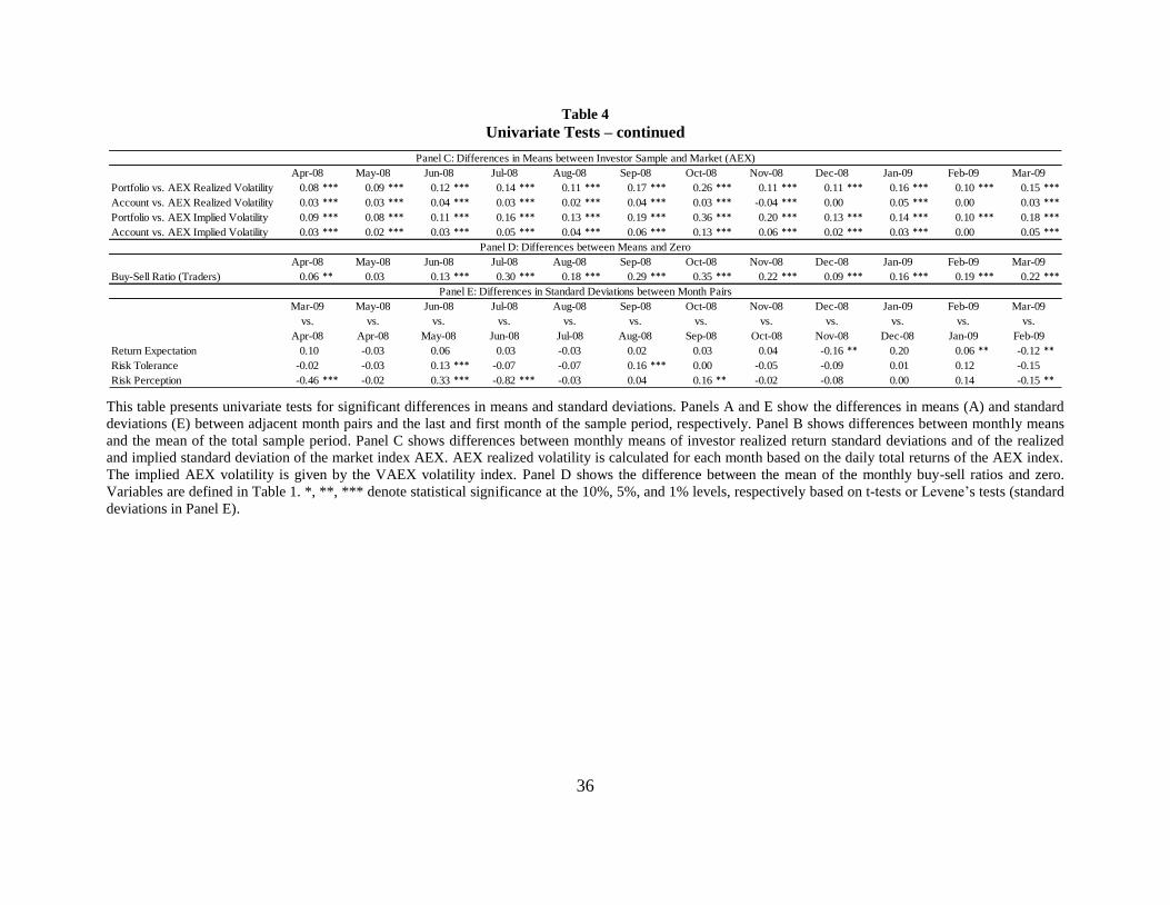
Investors’ return expectations (Figure 1) decrease significantly when investors experience a
month with bad returns (compare Table 4, Panel A). Return expectations reach their lowest level
during the height of the crisis (September–October 2008). In months with improving market
returns, however, return expectations recover significantly. Finally, towards the end of the
sample period (March 2009), their level cannot be statistically distinguished anymore from their
level at the beginning of the sample period (April 2008) (Table 4, Panel A). The recovery of
return expectations suggests that individual investors did not experience an enduring shock to
11
their return expectations as a result of the crisis, but instead regularly adapt their expectations to
changes in return experiences. Figure 1 highlights that return expectations (measured at the end
of each month) move in line with past market returns. The adaptive evolution of return
expectations during the crisis is similar to the adaptation process found in calmer market periods
(Hurd, van Rooij, and Winter 2011). Moreover, this finding is in line with De Bondt and Thaler’s
(1985) suggestion that investors overweigh the recent past when forming return expectations.
We find similar effects for risk tolerance and risk perception (Figure 2), though these
measures display less fluctuation over the sample period than return expectations. Both measures
become depressed especially in June (i.e., the first month with bad returns during the sample
period) and September 2008. In these months, the drop in the level of risk tolerance and increase
in the level of risk perception is significant compared to their levels in the previous months
(compare Table 4, Panel A). Both measures, however, already reach their lowest (risk tolerance)
and highest (risk perception) levels in June 2008 when compared to the average levels of these
measures during the complete sample period (Table 4, Panel B). Like investors’ return
expectations, both risk tolerance and risk perception recover towards the end of the sample
period. In fact, investors’ level of risk perception is significantly lower at the end of the sample
period as compared to the beginning of the sample period (compare Table 4, Panel A). Again, it
does not seem that the dramatic experiences of the financial crisis permanently decreased
(increased) individual investors’ risk tolerance (risk perception). Compared to other studies that
measure individual investor perceptions during the crisis (Bateman et al. 2011; Weber, Weber,
and Nosic 2012), this study’s longitudinal research design and frequent measurement offer
additional insights. Both Bateman et al. and Weber et al. measure investor perceptions during the
crisis less frequently and do not detect changes in risk tolerance and risk perceptions. Although
12
this study’s findings confirm the results of these other studies that risk tolerance and risk
perception are relatively stable over longer time intervals, we find that during the crisis period,
they significantly fluctuate and temporarily become depressed.
Overall, we find only limited support for hypothesis H1. During the financial crisis, investor
perceptions become depressed when the stock market does badly. That is, return expectations
and risk tolerance decrease, while at the same time, risk perceptions increase. However, the
depressing effect of the crisis on investors’ return expectations, risk tolerance, and risk
perceptions is temporarily as these variables recover with improving market returns. In fact, a
comparison of investor perceptions from the beginning of the sample period to the end of the
sample period shows that individual investors perceive less risk after the crisis than before the
crisis, while there are no significant changes in their return expectations and risk tolerance (Table
4, Panel A).
4.2 Investor Risk Taking during the Crisis
In this section we examine whether the financial crisis leads individual investors to reduce their
portfolio risk (H2). To measure portfolio risk, we use the volatility (standard deviation) of
investors’ daily portfolio returns. Figure 3 shows the monthly volatility of investor returns and
the realized as well as implied volatility of the market index (AEX). Investors’ monthly return
volatility tracks both measures of market volatility, while being significantly higher, on average
(Table 4, Panel C). Especially in October 2008, investors’ return volatility spikes (compare Table
4, Panels A and B). Thus, during the height of the crisis, investors are not de-risking their
portfolios. The sharp increase in market risk in this particular period may have come as a
surprise to investors. After October 2008, however, when market volatility decreases, individual
13
investors’ return volatility remains at a significantly higher level than that of the market (Table 4,
Panel C). Towards the end of the crisis, return volatility is even higher than at the beginning of
the crisis (Table 4, Panel A). Considering that individual investors are generally not well
diversified and hold only a limited number of different securities in their portfolios (cf.
Goetzmann and Kumar 2008), it might be difficult to reduce risk by changing portfolio
compositions. For 30% of the investors in our sample we have detailed portfolio information,
showing that, on average (median), they hold 13.1 (11.6) different securities. Thus, by selling a
particular risky security, idiosyncratic portfolio risk may actually go up. Furthermore,
considering general equilibrium effects, it might be difficult for individual investors to reduce
portfolio risk at a time when their trading counterparts (i.e., institutional investors) also try to
reduce risk (cf. Ben-David et al. 2012). Tests using additional information on the cash position in
investors’ accounts, however, confirm the previous results (Figure 3 and Table 4, Panels A and
B). Account volatility (i.e., the sum of the investment portfolio and cash) is generally lower than
portfolio volatility and also spikes at the height of the crisis. Account volatility is also
significantly higher towards the end of the crisis than at its beginning. Thus, at a time when it
might have been difficult to reduce risk within their investment portfolio, individual investors
also did not reduce risk by shifting from risky investments to cash.
[Figure 3 here]
Instead, individual investors used the depressed asset prices as a chance to enter the market.
Figure 4 shows individual investors’ monthly buy-sell ratio. Especially during September–
October 2008, the buy-sell ratio significantly increases compared to previous months (Table 4,
14
Panel A) as well as compared to the overall sample average (Table 4, Panel B). Generally, the
buy-sell ratio is significantly greater than zero, indicating net buying, on average (Table 4, Panel
D). This behavior of investors during the crisis mimics the findings of Kaniel, Saar, and Titman
(2008) for normal stock-market periods and those of Griffin et al. (2011) for the March 2000
technology stock reversal. That is, individual investors, on average, increase their buying volume
after price decreases (and vice-versa). In so doing, individual investors provided liquidity during
the falling market periods of the crisis while institutional investors withdrew liquidity (cf. Ben-
David et al. 2012).
[Figure 4 here]
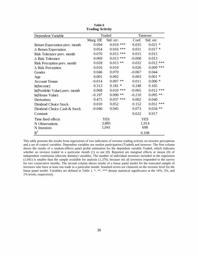
To gain more insight into the factors that drive individual investors’ risk-taking behavior, we
regress their portfolio standard deviation and buy-sell ratio on their perceptions. We run panel
regressions in which investor perceptions are included as explanatory variables in their one-
month lagged levels and changes (revisions) from that month to infer how perceptions at the start
of a month, and changes in perceptions during a month, influence behavior. This approach
differentiates the general effect of levels of investor perceptions (e.g., always having high risk
tolerance and high trading activity) from specific effects of revisions in perceptions and resulting
behavior. That is, we examine whether the monthly fluctuations in investor perceptions are an
important ingredient for understanding investor behavior, or whether only the levels of
perceptions matter. We control for other investor characteristics that prior literature suggests as
drivers of investor behavior, such as gender, age, account tenure, income, portfolio value, house
value, derivative usage, and dividend choice (Barber and Odean 2001; Dhar and Zhu 2006;
15
Bauer, Cosemans, and Eichholtz 2009; Seru, Shumway, and Stoffman 2010; Korniotis and
Kumar 2011b). We control for the possible impact of past aggregate market returns by including
time fixed effects (Section 5.3 provides robustness checks regarding investor-specific returns).6
Table 5 presents the results.
[Table 5 here]
Table 5 shows that studying the dynamics of investors’ perceptions leads to a better
understanding of their risk-taking behavior during the crisis. Both the levels of and revisions in
risk tolerance, as well as the levels of risk perception, are associated with risk taking. That is,
higher past levels of and upward revisions in risk tolerance lead investors to choose portfolios
with higher standard deviations. Furthermore, risk perceptions are positively associated with
portfolio risk, suggesting that individual investors are aware of the risk of their investment
portfolios. The regression coefficients are economically significant, as we examine monthly
standard deviations. For example, a one-point increase in the past level of risk perception is
associated with an increase in the annualized standard deviation of almost four percentage points.
The coefficients of the control variables are consistent with prior literature. Investors who
are more experienced (longer account tenure) and sophisticated (i.e., trade derivatives) take more
risk, while investors with larger portfolios take less risk (cf. Barber and Odean 2001; Bailey,
Kumar, and Ng 2008; Grinblatt and Keloharju 2009; Seru, Shumway, and Stoffman 2010).
With respect to the buy-sell ratio, we find that investors with higher levels of and upward
revisions in risk tolerance, lower levels of risk perception, less experience (shorter account
6 Standard errors are clustered on the investor level. Alternatively, we used Driscoll and Kraay (1998) standard
errors. Results in the latter specification are very similar in terms of coefficient significance (detailed results
available upon request), that is, the time fixed effect is picking up potential cross-sectional correlation.
16
tenure), more wealth (higher average house value), and lower levels of derivatives usage have a
higher buy-sell ratio (second column in Table 5). That is, more risk-tolerant investors increase
their market exposure, while investors who perceive higher risk lower their market exposure.
Overall, the results lead us to reject hypothesis H2. The financial crisis did not induce
individual investors to de-risk their portfolios. This behavior is rooted in the time-variation of
investor perceptions: risk tolerance quickly returns to pre-crisis levels while risk perception
levels are even lower at the end of the sample period than at the beginning of the sample period.
As these measures are key drivers of portfolio risk and buy-sell ratios, investors did not de-risk.
4.3 Investor Trading Activity during the Crisis
In this section we examine whether experiencing the final crisis led individual investors to
decrease (H3a) or increase (H3b) their trading activity. Figure 5 plots the fraction of investors that
trades each month and their turnover. The likelihood of trading and turnover significantly
increase during the height of the crisis, in particular in October 2008 (see Table 4, Panels A and
B). The increase in turnover is not a mechanical effect of falling portfolio values, as trading
volume also (marginally significantly) rises (compare Figure 6 and Table 4, Panels A and B).
[Figures 5-6 here]
The significant increase in trading activity during the height of the crisis makes it unlikely
that information overload (being associated with lower trading activity) plays a major role for
individual investors during the financial crisis. Increasing trading activity alone, however, is
insufficient to rule out potential information-overload effects. As a more formal test, we regress
17
investors’ trading activity on their perceptions and variables that previous research showed to be
linked to susceptibility to information overload. In particular, Agnew and Szykman (2005) find
that financially literate and experienced investors, that is, those with longer account tenure,
higher income, and larger portfolio values, suffer less from information overload. These
investors typically have less difficulty interpreting the frequent and sometimes conflicting
information that arrives during a crisis. Therefore, we expect them to have a lower tendency to
be overwhelmed by crisis events that could have led them to refrain from trading. If information
overload is present, trading activity (i.e., likelihood to trade and turnover) should be positively
related to variables that proxy for financial literacy and experience, such as account tenure,
income, and portfolio value. To examine this notion, we estimate two regression models
explaining investors’ likelihood of trading and turnover. As in Section 4.2, we control for a
variety of investor characteristics that prior literature identified as drivers of behavior and
include time fixed effects to control for the effect of past aggregate market returns (Section 5.3
provides robustness checks regarding investor-specific returns). Table 6 shows regression results.
Income is significantly and positively related to the likelihood to trade (consistent with an
information overload effect), but is not significantly related to turnover. Account tenure is
negatively associated with the likelihood to trade (not consistent with an information overload
effect), but is positively related with turnover (consistent with an information overload effect).
We find opposite results for the portfolio value coefficients. The results of Table 6 are consistent
with the intuition provided by Figure 5: the coefficient signs are sometimes in line but are also
often not in line with the theoretical predictions of information overload effects. It thus seems
unlikely that information overload played a major role for investor behavior during the crisis.
18
[Table 6 here]
As we do not find evidence in support of hypothesis H3a, we next test hypothesis H3b. That is, we
examine whether more reasons (changes in perceptions) and opportunities to trade (divergence of
perceptions) can explain the increase in trading activity, as observed in Figure 5. Both in the
likelihood of trading and the turnover regressions, most perception coefficients are significant
(Table 6). Exceptions are the coefficients for changes in risk perception (likelihood to trade), and
level and changes in risk tolerance (turnover). Overall, levels and changes in perceptions drive
trading activity. Figures 1 and 2 and Table 4 show that perceptions fluctuate significantly during
the crisis. Together with the regression results, this suggests that having more reasons to trade
leads investors to increase their trading activity. To measure divergence of perceptions (i.e.,
disagreement between different investors), we use the monthly cross-sectional standard deviation
of the perception measures (Doukas, Kim, and Pantzalis 2006; Zhang 2006; Güntay and
Hackbarth 2010; Banerjee 2011). Figure 6 plots the divergence of investor perceptions during the
crisis. Divergence of perceptions tends to move similarly as trading volume in most months. That
is, in months in which volume increases (June, September, August, however, not January),
divergence of perceptions also increases significantly (Table 4, Panel F). Overall, we thus find
support for H3b but reject H3a: the increased trading activity during the height of the crisis is
related to changes in perceptions as well as higher divergence of perceptions. In other words, the
crisis provided individual investors with more reasons as well as more opportunities to trade.
19
5. Robustness Checks and Tests of Alternative Explanations
5.1 Sample Selection Bias
A general concern with studies using surveys is that response behavior could be non-random. To
examine this issue, we first compare the investors that responded to the survey to the broker’s
overall investor population, followed by an analysis of the monthly variation of non-response.
As described in Section 3, brokerage records are available only for investors who responded
at least once to the survey. A limited amount of background information is available for all of the
broker’s clients for December 2005. This information includes their age, gender, portfolio value,
and number of trades. After imposing the same sample-selection restrictions for the broker’s
complete client base as for the 2008–2009 survey respondents (see Section 3), we have 2005
background information for 35,122 investors in total, of which 742 are also respondents to the
2008–2009 survey. A comparison of the 742 survey respondents with all of the broker’s clients
based on the 2005 data shows that 2008–2009 survey respondents are, on average, more likely to
be male (95% vs. 91%, p = 0.000) and older (3.25 years, p = 0.000), have larger portfolios
(€10.956, p = 0.000), and are more likely to trade (55% vs. 39%, p = 0.000). No significant
differences are found regarding their number of trades (given that they traded).
In the following, the characteristics of all investors who responded to the 2008–2009 survey
are compared with those of the non-responding investors for each month using the 2008–2009
brokerage-account data. Additionally, to examine whether non-response is related to investor
behavior or performance, investors’ trading and risk-taking variables, returns, Sharpe ratios, and
alphas are analyzed. Comparing respondent with non-respondent means shows that in some
months there are significant differences, especially with respect to age, account tenure, and
trading activity (detailed results available upon request). In these months, respondents, compared
20
to non-respondents, are older, have longer account tenure, and are more likely to trade, whereas
their overall transaction volume is smaller. That is, based on the 2008–2009 data, similar
tendencies with respect to response behavior emerge as with the 2005 data. This indicates that
investors that responded to the survey only a few times mimic investors that did not respond at
all. Except for August 2008 (alpha) and December 2008 (Sharpe ratio) there are no significant
differences between respondents and non-respondents regarding risk taking or performance.
Thus, response behavior is unlikely to be driven by these investor characteristics. When
examining the months with significant differences between respondents and non-respondents
regarding overall market performance, no patterns emerge that indicate that response behavior
would be driven by overall market developments.
To statistically account for the identified differences between respondents and non-
respondents, as well as the monthly variation in significant differences, as a robustness check an
inverse-probability-weighted estimator is applied (Robins and Rotnitzky 1995; Wooldridge
2002). For each of the 12 months, a logit model is estimated where the dependent variable
indicates either response (1) or non-response (0). As explanatory variables, we include the set of
variables as discussed above. Next, the predicted probabilities of survey response are calculated.
Finally, all regression models of Section 4 are estimated again using the inverse of the predicted
probabilities as sample weights. The results of the regressions that include this estimator are
similar to those obtained from the original specifications in terms of coefficient magnitudes,
significance, and signs (detailed results available upon request). That is, in general our results are
not impacted by non-random response behavior problems. Exceptions are the turnover regression
where we identify that, compared to male investors, female investors have lower turnover ( = -
0.075, p = 0.085), and the portfolio risk regression, where we find that female investors hold less
21
risky portfolios ( = -0.036, p = 0.048). Both results are consistent with the findings of Barber
and Odean (2001).
5.2 Response Timing Bias
Besides sample selection considerations, response timing might impact the results. Large
differences in the point in time at which investors respond to the survey might affect the results
due to the rapidly changing market conditions during the crisis. Therefore, we first check the
monthly distributions of survey response time. Generally, investors complete the survey shortly
after they received the monthly invitation email: 31% of responses occur on the same day that
the survey email is sent. Within another day, 53% of the total number of responses is received,
after five days 85%, and after ten days 95% of total survey responses are received. The clustering
of responses within the first few days after each survey email was sent makes it unlikely that
there is a response-time pattern in the data that could introduce a possible bias. Nevertheless, to
check more carefully for this possibility, all regression models of Section 4 are estimated again.
Yet, we now exclude investors with long response durations (more than five days, or
alternatively, more than ten days from the day the survey email was sent). The results of these
regressions are similar to those obtained from the original specifications in terms of coefficient
magnitudes, significance, and signs (detailed results available upon request). One exception is
the portfolio risk regression, where removing investors with a response duration of either more
than five or ten days, leads the coefficient for the change in risk tolerance to be significant only
at the 5% level (this was 1% before excluding late responders).
22
5.3 Investor Perceptions versus Past Returns as Drivers of Behavior
Figures 1 and 2 suggest that the month-to-month changes (revisions) in investors’ perceptions
follow changes in the Dutch stock market index (AEX). In particular, revisions in return
expectation and risk tolerance seem to be positively, and revisions in risk perception negatively,
associated with changes in market returns. Hence, one could hypothesize that perceptions have a
significant effect in the regression analyses only because they reflect past returns (cf. Statman,
Thorley, and Vorkink 2006; Barber, Odean, and Zhu 2007; Nicolosi, Peng, and Zhu 2009).
To examine this alternative explanation, we examine the within-investor correlations of the
levels of and revisions in perceptions with the levels of and changes in the market and individual
investor returns, respectively. Since perceptions are measured at the end of each month, while
returns are realized over the course of each month, we examine the contemporaneous
correlations to detect an impact of past returns on current perceptions. The results show that
although the levels and changes in perceptions are correlated with both the levels and changes in
the market and individual investor returns, all correlations are relatively low and far from unity
(detailed results available upon request). This gives first evidence that investors’ perceptions
provide additional information over and beyond the information included in their past returns.
In addition, we break down the changes in investor perceptions on a monthly basis and
distinguish between investors with positive and negative past returns, as well as changes in past
returns. The results show that, in most months, average return expectations and risk tolerance
move in the same direction, while risk perceptions move in the opposite direction of both market
returns and individual investor returns (detailed results available upon request). There is,
however, considerable heterogeneity between the directions of investors’ changes in perceptions.
23
The maximum percentage of investors that changes perceptions in line with the average change
of the overall sample of investors is 77% (= negative change in return expectations in June
2008). In most months, this percentage is lower than 60%. Furthermore, when looking closer at
individual investor returns, which may be the source of heterogeneity of the direction of changes
in investor perceptions, it becomes clear that it is not only individuals’ past return experience that
drives changes in their perceptions. The results show that the fraction of investors that change
their perceptions in line with the change in the overall market return is larger among investors
with an individual return experience that matches the sign (direction) of the market return
(change). Thus, investor perceptions are partially influenced by past individual returns. The
effect of past individual returns is small, however, because the difference between the fractions
of investors with positive and negative individual return experience that change perceptions in
line with the market is less than 10 percentage points (detailed results available upon request).
Finally, we analyze the impact of investor past return experience versus investor perceptions
on their trading and risk-taking behavior. Since the possible impact of the past market return
(AEX) on investor behavior is already accounted for by the time fixed effects that are included in
the regression models of Section 4, only the possible impact of individual investor return
experience is examined further. For this, we again estimate the regression models including
investors’ past returns, change in past returns, or both, as control variables. The results show that
the levels of investors’ past returns have no significant effect in any of the regression models.
Changes in investors’ past returns do impact behavior, but including them does not eliminate the
explanatory power of investor perceptions (detailed results available upon request). Consistent
with Statman et al.’s (2006) findings, changes in investors’ past returns have a significant effect
in the turnover regression ( = 0.013, p = 0.004), which also includes past returns as a control
24
variable, and in the buy-sell ratio regression models that include only the investors’ change in
past returns, as well as both the past returns and change in past returns ( = 0.011, p = 0.000 in
both models). The significance, signs, and approximate magnitudes of the investor perception
coefficients do not change in any of the regression models. The only exception is that in the risk-
taking (standard deviation of portfolio return) regression models that include the change in past
returns, or both the past returns and the change in past returns, the coefficient for the change in
risk perception becomes significant and positive ( = 0.009, p = 0.072 in both models). Overall,
the analyses of this section show that investor perceptions not only pick up information from past
returns, but they also provide explanatory power for investor behavior well beyond the
previously documented effect of past returns and changes in past returns.
5.4 Relevance of Investor Risk-Taking and Trading Behavior During the Crisis
Results of Section 4 show that investor perceptions and fluctuations therein are important drivers
of investor behavior. The aspects of trading and risk-trading behavior that we study have been
shown to be related to investor performance during normal market periods. Thus, economically,
they matter. In this section we assess whether, also during the financial crisis, the behavioral
variables that we study are related to investor performance, and thus have relevance in this
particular period. To do so, we regress three measures of investor performance on investor
behavior and a set of controls. As performance measures, we study investors’ monthly portfolio
return, their monthly Sharpe-Ratio, and their monthly one-factor (Jensen’s) alpha.7 The aspects
of investor behavior that we include are based on Section 4: we examine the impact of the
7 We cannot estimate multi-factor alphas because of limitations on the portfolio-holdings data. Daily market-value
data on the portfolio level is available for all investors. Detailed portfolio component data, however, is only
available for a subset of 30% of the investors. But even in that case, only the name of the security, the indication of
the asset class, and the historical purchase prices are available for each portfolio component.
25
standard deviation of investors’ portfolio return, as well as that of their buy-sell ratio, likelihood
to trade, and turnover. Note that, since investment risk is already accounted for in the dependent
variable in the Sharpe-Ratio and alpha regression, only in the portfolio-return regression do we
include the standard deviation of returns as an independent variable. The results of Table 7 show
that the behavioral variables that we consider in this paper are important drivers of investor
performance during the financial crisis. As overall market returns were mostly negative during
the sample period, both portfolio risk (standard deviation) and the buy-sell ratio are negatively
associated with performance. In addition, trading activity (turnover), is negatively related to
performance, consistent with results obtained in normal market periods (Barber and Odean
2000). Overall, these regression results provide evidence that the investor behaviors that we
study during the financial crisis are economically relevant.
[Table 7 here]
6. Conclusion
We combine monthly survey data with matching brokerage records and show how individual
investor perceptions change and drive trading and risk-taking behavior during the 2008–2009
financial crisis. Investor perceptions exhibit significant fluctuation over the course of the crisis,
with risk tolerance and risk perceptions being less volatile than return expectations. In the worst
months of the crisis, investors’ return expectations and risk tolerance decrease, while their risk
perceptions increase. Towards the end of the crisis, return expectations, risk tolerance, and risk
perceptions recover. We find substantial swings in trading and risk-taking behavior during the
crisis that are driven by changes in investor perceptions. Contrary to popular beliefs and
26
expectations from prior literature, however, individual investors continue to trade and do not de-
risk their investment portfolios during the crisis. Individual investors also do not try to reduce
risk by shifting from risky investments to cash. Instead, individual investors use the depressed
asset prices as a chance to enter the stock market.
This study provides two insights for asset pricing. First, consistent with the recent work of
Guiso, Sapienza and Zingales (2011), we show that investor’s risk tolerance is time-varying (see
Figure 2 and Table 4, Panels A and B) and significantly related to risk-taking behavior (see the
risk-taking regression). Investor’s portfolio risk, however, seems to move in parallel with market
risk (see Figure 3), as if changes in risk tolerance had no impact. Hence, it may be investor
inertia, that is, the large fraction of investors not trading during the sample period (see Figure 5),
as well as rebalancing behavior after price changes (see Figure 4 and the buy-sell ratio
regression), that ultimately drives portfolio risk. Thus, although present, time-varying risk
tolerance and its impact on risk-taking behavior can be masked and overcompensated by the
impact of investor inertia found by Brunnermeier and Nagel (2008) as well as Bilias,
Georgarakos, and Haliassos (2010). Second, although the sample period does not cover the time
before the financial crisis, this paper’s findings on the evolution of investor perceptions do shed
light on the psychological factors contributing to the asset-price bubble preceding the crisis.
Barberis (2011), for example, argues that the representativeness heuristic is largely responsible
for the overly optimistic pre-crisis expectation formation. This paper’s results show that
individual investor perceptions indeed exhibit adaptive behavior with respect to very recent
stock-market performance (see Figures 1-2). We thus provide empirical support for Barberis’s
(2011) theoretical viewpoint regarding the psychological factors that contribute to the creation of
financial bubbles in general and to the financial crisis of 2008–2009 in specific.
27
References
Agnew, J. R. and L. R. Szykman (2005), "Asset Allocation and Information Overload: The
Influence of Information Display, Asset Choice, and Investor Experience," Journal of
Behavioral Finance, 6(2), 57-70.
Aloui, R., M. S. Ben Aïssa, and D. K. Nguyen (2011), "Global Financial Crisis, Extreme
Interdependences, and Contagion Effects: The Role of Economic Structure?," Journal of
Banking and Finance, 35(1), 130-141.
Bailey, W., A. Kumar, and D. Ng (2008), "Foreign Investments of U.S. Individual Investors:
Causes and Consequences," Management Science, 54(3), 443-459.
Bailey, W., A. Kumar, and D. Ng (2011), "Behavioral Biases of Mutual Fund Investors," Journal
of Financial Economics, 102(1), 1-27.
Banerjee, S. (2011), "Learning from Prices and the Dispersion in Beliefs," Review of Financial
Studies, 24(9), 3025-3068.
Barber, B. M. and T. Odean (2000), "Trading is Hazardous to Your Wealth: the Common Stock
Investment Performance of Individual Investors," Journal of Finance, 55(2), 773-806.
Barber, B. M. and T. Odean (2001), "Boys Will be Boys: Gender, Overconfidence, and Common
Stock Investment," Quarterly Journal of Economics, 116(1), 261-292.
Barber, B. M., T. Odean, and N. Zhu (2007), "Systematic Noise," Journal of Financial Markets,
12(4), 547-569.
Barberis, N. (2011), "Psychology and the Financial Crisis of 2007-2008," working paper,
Available at SSRN: http://ssrn.com/abstract=1742463.
Bateman, H., J. Louviere, S. Satchell, T. Islam, and S. Thorp (2011), "Retirement Investor Risk
Tolerance in Tranquil and Crisis Periods: Experimental Survey Evidence," Journal of
Behavioral Finance, 12(4), 201-218.
Bauer, R., M. Cosemans, and P. M. A. Eichholtz (2009), "Option Trading and Individual
Investor Performance," Journal of Banking and Finance, 33(4), 731-746.
Baur, D. G. (2012), "Financial Contagion and the Real Economy," Journal of Banking and
Finance, In Press.
Ben-David, I., F. Franzoni, and R. Moussawi (2012), "Hedge Fund Stock Trading in the
Financial Crisis of 2007–2009," Review of Financial Studies, 25(1), 1-54.
Bilias, Y., D. Georgarakos, and M. Haliassos (2010), "Portfolio Inertia and Stock Market
Fluctuations," Journal of Money, Credit and Banking, 42(4), 715-742.
Bricker, J., B. K. Bucks, A. Kennickell, T. L. Mach, and K. Moore (2011), "Drowning or
Weathering the Storm? Changes in Family Finances From 2007 to 2009," NBER Working
Paper No.16985.
Brunetti, C. M., M. di Filippo, and J. H. Harris (2011), "Effects of Central Bank Intervention on
the Interbank Market During the Subprime Crisis," Review of Financial Studies, 24(6),
2053-2083.
28
Brunnermeier, M. K. and S. Nagel (2008), "Do Wealth Fluctuations Generate Time-Varying
Risk Aversion? Micro-Evidence on Individuals' Asset Allocation," American Economic
Review, 98(3), 713-736.
Campello, M., J. R. Giambona, J. R. Graham, and C. R. Harvey (2011), "Liquidity Management
and Corporate Investment During a Financial Crisis," Review of Financial Studies, 24(6),
1944-1979.
Cronbach, L. J. (1951), "Coefficient Alpha and the Internal Structure of Tests," Psychometrika,
16(3), 297-334.
De Bondt, W. F. M. and R. H. Thaler (1985), "Does the Stock Market Overreact?," Journal of
Finance, 40(3), 793-805.
Demyanyk, Y. and O. Van Hemert (2011), "Understanding the Subprime Mortgage Crisis,"
Review of Financial Studies, 24(6), 1848-1880.
Dhar, R. and N. Zhu (2006), "Up Close and Personal: Investor Sophistication and the Disposition
Effect," Management Science, 52(5), 726-740.
Dillon, W. R. and R. McDonald (2001), "How to Combine Multiple Items into a Composite
Score," Journal of Consumer Psychology, 10(1/2), 62-64.
Dorn, D. and P. Sengmueller (2009), "Trading as Entertainment?," Management Science, 55(4),
591-603.
Doukas, J. A., C. Kim, and C. Pantzalis (2006), "Divergence of Opinion and Equity Returns,"
Journal of Financial and Quantitative Analysis, 41(3), 573-606.
Driscoll, J. C. and A. C. Kraay (1998), "Consistent Covariance Matrix Estimation with Spatially
Dependent Panel Data," Review of Economics and Statistics, 80(4), 549-560.
Dzielinski, M. (2011), "When Does Company-Specific News Matter? Determinants of News-
Related Stock Returns," working paper, University of Zurich.
Eurostat (2011), "Distribution of Population by Tenure Status, Type of Household and Income
Group," retrieved from
http://appsso.eurostat.ec.europa.eu/nui/show.do?dataset=ilc_lvho02&lang=en.
Foucault, T., D. Sraer, and D. J. Thesmar (2011), "Individual Investors and Volatility," Journal
of Finance, 66(4), 1369-1406.
Gervais, S. and T. Odean (2001), "Learning to be Overconfident," Review of Financial Studies,
14(1), 1-27.
Glaser, M. and M. Weber (2005), "September 11 and Stock Return Expectations of Individual
Investors," Review of Finance, 9(2), 243-279.
Glaser, M. and M. Weber (2007), "Why Inexperienced Investors do not Learn: They do not
Know their past Portfolio Performance," Finance Research Letters, 4 203-216.
Goetzmann, W. N. and A. Kumar (2008), "Equity Portfolio Diversification," Review of Finance,
12(3), 433-463.
Griffin, J. M., J. H. Harris, T. Shu, and S. Topaloglu (2011), "Who Drove and Burst the Tech
Bubble?," Journal of Finance, 66(4), 1251-1290.
29
Grinblatt, M. and M. Keloharju (2009), "Sensation Seeking, Overconfidence, and Trading
Activity," Journal of Finance, 64(2), 549-578.
Guiso, L., P. Sapienza, and L. Zingales (2011), "Time Varying Risk Aversion," working paper.
Güntay, L. and D. Hackbarth (2010), "Corporate Bond Credit Spreads and Forecast Dispersion,"
Journal of Banking and Finance, 34(10), 2328-2345.
Hair, J. F., R. E. Anderson, R. L. Tatham, and W. C. Black (1998), Multivariate Data Analysis.
Upper Saddle River, New Jersey: Prentice Hall.
Harris, M. and A. Raviv (1993), "Differences of Opinions Make a Horse Race," Review of
Financial Studies, 6(3), 473-506.
Hirshleifer, D. (2001), "Psychology and Asset Pricing," Journal of Finance, 56(4), 1533-1597.
Hurd, M., M. van Rooij, and J. Winter (2011), "Stock Market Expectations of Dutch
Households," Journal of Applied Econometrics, 26(3), 416-436.
Ivashina, V. and D. S. Scharfstein (2010), "Bank Lending during the Financial Crisis of 2008,"
Journal of Financial Economics, 97(3), 319-339.
Jin, J. Y., K. Kanagaretnam, and G. J. Lobo (2011), "Ability of Accounting and Audit Quality
Variables to Predict Bank Failure During the Financial Crisis," Journal of Banking and
Finance, 35(11), 2811-2819.
Kahneman, Daniel and Amos Tversky (1972), "Subjective Probability: A Judgment of
Representativeness," Cognitive Psychology, 3(3), 430-454.
Kaniel, R., G. Saar, and S. Titman (2008), "Individual Investor Trading and Stock Returns,"
Journal of Finance, 63(1), 273-310.
Kapteyn, A. and F. Teppa (2011), "Subjective Measures of Risk Aversion, Fixed Costs, and
Portfolio Choice," Journal of Economic Psychology, 32(4), 564-580.
Kogan, L., S. A. Ross, J. Wang, and M. M. Westerfield (2006), "The Price Impact and Survival
of Irrational Traders," Journal of Finance, 61(1), 195-229.
Korniotis, G. M. and A. Kumar (2011a), "Do Behavioral Biases Adversely Affect the Macro-
Economy?," Review of Financial Studies, 24(5), 1513-1559.
Korniotis, G. M. and A. Kumar (2011b), "Do Older Investors Make Better Investment
Decisions?," Review of Economics and Statistics, 93(1), 244-265.
Kumar, A. and C. Lee (2006), "Retail Investor Sentiment and Return Comovements," Journal of
Finance, 61(5), 2451-2486.
Lam, C. F., D. S. DeRue, E. P. Karam, and J. R. Hollenbeck (2011), "The Impact of Feedback
Frequency on Learning and Task Performance: Challenging the "More is Better"
Assumption," Organizational Behavior and Human Decision Processes, 116(2), 217-228.
Lee, C. M. C., A. Shleifer, and R. H. Thaler (1991), "Investor Sentiment and the Closed-End
Fund Puzzle," Journal of Finance, 46(1), 75-109.
Longstaff, F. A. (2010), "The Subprime Credit Crisis and Contagion in Financial Markets,"
Journal of Financial Economics, 97(3), 436-450.
30
Maddaloni, A. and J.-L. Peydró (2011), "Bank Risk-taking, Securitization, Supervision, and
Low-interest Rates: Evidence from the Euro Area and the U.S. Lending Standards," Review
of Financial Studies, 24(6), 2121-2165.
Malmendier, U. and S. Nagel (2011), "Depression Babies: Do Macroeconomic Experiences
Affect Risk-Taking?," Quarterly Journal of Economics, 126(1), 373-416.
Moshirian, F. (2011), "The Global Financial Crisis and the Evolution of Markets, Institutions,
and Regulation," Journal of Banking and Finance, 35(3), 502-511.
Netemeyer, R. G., W. O. Bearden, and S. Sharma (2003), Scaling Procedures: Issues and
Applications. Thousand Oaks, California: Sage Publications.
Nicolosi, G., L. Peng, and N. Zhu (2009), "Do Individual Investors Learn from their Trading
Experience?," Journal of Financial Markets, 12(2), 317-336.
Nunnally, J. C. and I. H. Bernstein (1994), Psychometric Theory. New York: McGraw-Hill.
Pennings, J. M. E. and A. Smidts (2000), "Assessing the Construct Validity of Risk Attitude,"
Management Science, 46(10), 1337-1348.
Pennings, J. M. E. and B. Wansink (2004), "Channel Contract Behavior: The Role of Risk
Attitudes, Risk Perceptions, And Channel Members' Market Structures," Journal of
Business, 77(4), 697-723.
Robins, J. M. and A. Rotnitzky (1995), "Semiparametric Efficiency in Multivariate Regression
Models," Journal of the American Statistical Association, 90(429), 122-129.
Rouwendal, J. (2007), "Mortgage interest deductibility and homeownership in the Netherlands,"
Journal of Housing and the Build Environment, 22(4), 369-382.
Santos, J. A. C. (2011), "Bank Corporate Loan Pricing Following the Subprime Crisis," Review
of Financial Studies, 24(6), 1916-1943.
Seru, A., T. Shumway, and N. Stoffman (2010), "Learning by Trading," Review of Financial
Studies, 23(2), 705-739.
Shell, A. (2010), "Could investors fleeing stocks become a lost generation?," USA Today,
September 2, 2010.
Statman, M., S. Thorley, and K. Vorkink (2006), "Investor Overconfidence and Trading
Volume," Review of Financial Studies, 19(4), 1531-1565.
Steverman, B. (2009), "Financial Crisis Leaves Investors Wary of Risk," Bloomberg
Businessweek, September 13, 2009.
Thaler, R. H. and E. J. Johnson (1990), "Gambling With the House Money and Trying to Break
Even: The Effects of Prior Outcomes on Risky Choice," Management Science, 36(6), 643-
660.
Weber, M., E. U. Weber, and A. Nosic (2012), "Who Takes Risks When and Why: Determinants
of Changes in Investor Risk Taking," Review of Finance, Forthcoming.
Wooldridge, J. M. (2002), "Inverse Probability Weighted M-Estimation for Sample Selection,
Attrition, and Stratification," Portuguese Economic Journal, 1(2), 117-139.
Zhang, X. F. (2006), "Information Uncertainty and Stock Returns," Journal of Finance, 61(1),
105-136.
31
Table 1
Variable Definitions
Variable Definition
Gender Indicator variable taking the value 0 for male investors and 1 for female investors.
Age Age of the investor in years as of April 2008.
Account Tenure Account tenure of the investor in years as of April 2008.
Income Annual disposable income in 2007 (= gross income minus taxes, social security
contributions, health insurance premiums paid) per person receiving income. Assigned to
each investor based on their 6-digit postal code (= average net income per postal code
from Statistics Netherlands). This postal code is unique for each street in the Netherlands.
Portfolio Value Value of investment assets in an investor’s account at the end of the month.
House Value Value of house in 2008. Assigned to each investor based on their 6-digit postal code.
This postal code is unique for each street in the Netherlands. Data source is the average
residential house value per 6-digit postal code from Statistics Netherlands.
Derivatives Indicator variable taking the value 1 if an investor traded an option or futures contract at
least once during the sample period or 0 otherwise.
Traded Indicator variable taking the value 1 if an investor traded in a particular month or 0
otherwise.
Trades Number of all executed transactions in a particular month.
Volume Sum of the absolute values of all purchases and sales in a particular month.
Turnover Average of the absolute values of all purchases and sales in a particular month divided by
the average of the portfolio values at the beginning and end of a particular month.
Dividend Choice Stock Indicator variable taking the value 1 if the investor's preferred way to receive dividend is
stock dividend or 0 in case of a preference for cash dividend.
Dividend Choice Cash &
Stock
Indicator variable taking the value 1 if the investor's preferred way to receive dividend is
stock dividend for one of her subaccounts and cash for another subaccount or 0 in case of
a preference for cash dividend for all her subaccounts.
Buy-Sell Ratio Difference between volume buy and volume sell, divided by volume. For investors with
no trades in a particular month, this ratio is set to zero (such investors mimic an investor
with equal buy and sell volume).
Return Monthly investor return given by the product of the daily relative changes in the value of
her portfolio after transaction costs and portfolio in- and outflows.
Portfolio Volatility Investor realized monthly portfolio volatility calculated based on the daily returns on
investor portfolios.
Account Volatility Investor realized monthly account volatility calculated based on the daily returns on
investor account values (= portfolio value + cash).
Sharpe Ratio Monthly return divided by portfolio volatility (in monthly terms).
Alpha One-factor alpha (Jensen’s alpha) in a particular month (in monthly terms).
Return Expectation Reflects how optimistic a respondent is about her investment portfolio and its returns in
the upcoming month (see Table 3).
Risk Tolerance Reflects a respondent’s general predisposition toward financial risk (see Table 3).
Risk Perception Reflects a respondent’s interpretation of how risky the stock market will be in the
upcoming month (see Table 3).
Because of data availability, the data retrieved from Statistics Netherlands refer to different years. That is, to 2007
for the income data, and to 2008 for the house value data.
32
Table 2
Descriptive Statistics
Month Apr-08 May-08 Jun-08 Jul-08 Aug-08 Sep-08 Oct-08 Nov-08 Dec-08 Jan-09 Feb-09 Mar-09
Investors N 1,376 1,376 1,376 1,376 1,376 1,376 1,376 1,376 1,376 1,376 1,376 1,376
Gender mean 0.08 0.08 0.08 0.08 0.08 0.08 0.08 0.08 0.08 0.08 0.08 0.08
Age mean 50.56 50.56 50.56 50.56 50.56 50.56 50.56 50.56 50.56 50.56 50.56 50.56
Age std 13.57 13.57 13.57 13.57 13.57 13.57 13.57 13.57 13.57 13.57 13.57 13.57
Account Tenure mean 4.07 4.07 4.07 4.07 4.07 4.07 4.07 4.07 4.07 4.07 4.07 4.07
Account Tenure std 2.77 2.77 2.77 2.77 2.77 2.77 2.77 2.77 2.77 2.77 2.77 2.77
Income € mean 20,242 20,242 20,242 20,242 20,242 20,242 20,242 20,242 20,242 20,242 20,242 20,242
Income € std 4,314 4,314 4,314 4,314 4,314 4,314 4,314 4,314 4,314 4,314 4,314 4,314
Portfolio Value € mean 52,854 52,695 44,872 42,840 45,963 37,688 31,127 30,100 30,679 29,564 26,514 27,875
Portfolio Value € std 156,058 156,096 134,883 127,338 135,203 117,935 101,325 104,663 105,279 99,322 91,598 92,307
House Value € mean 278,982 278,982 278,982 278,982 278,982 278,982 278,982 278,982 278,982 278,982 278,982 278,982
House Value € std 112,278 112,278 112,278 112,278 112,278 112,278 112,278 112,278 112,278 112,278 112,278 112,278
Fraction Derivatives 0.39 0.39 0.39 0.39 0.39 0.39 0.39 0.39 0.39 0.39 0.39 0.39
Fraction Traded 0.46 0.47 0.48 0.47 0.41 0.51 0.63 0.42 0.37 0.41 0.40 0.42
Trades (Traders) mean 8.57 7.54 7.71 9.24 7.16 8.72 10.60 8.83 7.81 9.64 8.87 10.13
Trades (Traders) std 11.38 11.15 12.44 16.75 10.63 13.06 16.65 13.10 12.04 14.66 14.86 17.75
Volume € (Traders) mean 48,067 30,260 33,038 36,312 30,861 41,439 51,042 31,225 22,919 28,506 26,003 29,593
Volume € (Traders) std 202,150 70,839 95,236 113,827 98,506 147,420 275,317 107,946 63,888 78,723 77,374 97,800
Turnover (Traders) mean 0.55 0.46 0.42 0.60 0.46 0.62 0.99 0.73 0.61 0.80 0.67 0.78
Turnover (Traders) std 1.53 1.22 1.12 1.85 1.41 1.87 3.63 1.82 1.82 2.77 2.49 2.46
Panel A: All Brokerage Accounts
33
Table 2
Descriptive Statistics – continued
Month Apr-08 May-08 Jun-08 Jul-08 Aug-08 Sep-08 Oct-08 Nov-08 Dec-08 Jan-09 Feb-09 Mar-09
Investors N 787 701 605 557 520 491 650 402 330 312 272 291
Gender mean 0.07 0.08 0.08 0.08 0.08 0.08 0.09 0.08 0.08 0.08 0.09 0.09
Age mean 50.55 51.22 51.50 51.83 52.79 52.60 51.50 52.31 52.65 52.64 53.83 53.25
Age std 13.51 13.55 13.43 13.57 12.90 13.05 13.29 13.25 12.88 12.86 12.62 12.67
Account Tenure mean 3.93 3.98 4.09 3.98 4.11 4.08 4.26 4.35 4.34 4.45 4.53 4.38
Account Tenure std 2.76 2.79 2.77 2.78 2.77 2.76 2.78 2.73 2.75 2.74 2.68 2.71
Income € mean 20,181 20,088 20,109 19,978 20,085 20,002 20,147 19,892 19,859 20,046 20,034 20,028
Income € std 4,285 3,956 4,240 3,729 3,835 4,153 4,197 3,808 3,543 3,897 3,844 3,860
Portfolio Value € mean 54,446 54,264 45,411 45,509 49,557 39,707 29,490 33,660 30,169 30,693 27,444 27,229
Portfolio Value € std 143,872 144,617 128,455 128,159 124,176 105,507 100,216 118,529 66,600 66,198 53,089 55,039
House Value € mean 276,690 272,969 272,038 273,559 274,221 274,736 277,543 272,429 272,020 273,443 277,193 273,037
House Value € std 110,125 102,015 109,290 101,943 101,006 110,771 112,864 104,787 98,530 99,506 108,672 100,576
Fraction Derivatives 0.41 0.42 0.43 0.42 0.44 0.44 0.37 0.38 0.41 0.45 0.41 0.41
Fraction Traded 0.52 0.54 0.55 0.52 0.46 0.54 0.64 0.46 0.42 0.48 0.49 0.45
Trades (Traders) mean 9.23 7.08 7.94 8.40 6.68 8.54 10.79 8.66 7.23 10.20 10.08 9.72
Trades (Traders) std 12.26 10.79 11.90 12.57 9.58 13.76 18.50 12.51 10.33 16.10 16.88 13.97
Volume € (Traders) mean 56,262 24,814 31,821 27,447 22,637 28,375 55,642 30,555 22,986 35,797 31,304 27,663
Volume € (Traders) std 242,164 53,239 80,947 65,300 48,199 65,511 359,009 87,480 69,731 93,522 84,222 73,659
Turnover (Traders) mean 0.65 0.43 0.49 0.57 0.36 0.50 1.10 0.86 0.47 0.56 0.70 1.00
Turnover (Traders) std 1.82 1.13 1.41 1.61 0.91 1.08 4.68 2.23 1.51 1.07 2.08 3.91
Return Expectation mean 4.35 4.22 3.68 3.93 4.27 3.53 3.41 3.73 3.93 4.13 3.61 4.36
Return Expectation std 0.93 0.90 0.96 1.00 0.96 0.99 1.01 1.05 0.89 1.09 1.15 1.03
Risk Tolerance mean 4.03 4.02 3.64 3.90 4.08 3.71 3.85 3.97 4.03 3.95 3.98 4.04
Risk Tolerance std 1.15 1.13 1.26 1.19 1.12 1.28 1.28 1.23 1.14 1.15 1.28 1.13
Risk Perception mean 4.47 4.46 5.02 4.19 3.93 4.49 4.31 4.34 4.12 4.13 4.50 4.25
Risk Perception std 1.66 1.64 1.96 1.14 1.11 1.15 1.31 1.28 1.21 1.21 1.35 1.20
Panel B: Survey Respondents
This table presents monthly summary statistics for the brokerage account data. Panel A refers to all investors for whom brokerage records are available. This
sample includes investors who participated at least once during the entire sample period in the survey and who were not excluded by the sample-selection
restrictions as defined in Section 3. The monthly summary statistics presented in Panel B refer to the subset of investors who responded to the survey in each
respective month. Variables are defined in Table 1.
34
Table 3
Survey Questions
This table presents the questions as used in this study’s monthly surveys. A 7-point Likert scale is used to record
investors’ response to each question. Each survey variable (i.e., return expectation, risk tolerance, risk perception) is
calculated as the equally weighted average of the respective survey questions. * denotes a reverse-scored question.
Survey Variable Answer Categories
Return Expectation (1 = low/pessimistic, 7 = high/optimistic)
Next month, I expect my investments to do less well than desired. 1 (totally agree)–7 (totally disagree)
For the next month, I have a positive feeling about my financial
future.*
1 (totally agree)–7 (totally disagree)
Next month, my investments will have a worse performance than
those of most other investors.
1 (totally agree)–7 (totally disagree)
Next month, it is unlikely that my investment behavior will lead to
positive returns.
1 (totally agree)–7 (totally disagree)
For the next month, the future of my investment portfolio looks
good.*
1 (totally agree)–7 (totally disagree)
Risk Tolerance (1 = low risk tolerance, 7 = high risk tolerance)
Next month, I prefer certainty over uncertainty when investing. 1 (totally agree)–7 (totally disagree)
Next month, I avoid risks when investing. 1 (totally agree)–7 (totally disagree)
Next month, I do not like to take financial risks. 1 (totally agree)–7 (totally disagree)
Next month, I do not like to “play it safe” when investing.* 1 (totally agree)–7 (totally disagree)
Risk Perception (1 = low perceived risk, 7 = high perceived risk)
I consider investing to be very risky next month.* 1 (totally agree)–7 (totally disagree)
I consider investing to be safe next month. 1 (totally agree)–7 (totally disagree)
I consider investing to be dangerous next month. * 1 (totally agree)–7 (totally disagree)
I consider investing to have little risk next month. 1 (totally agree)–7 (totally disagree)
35
Table 4
Univariate Tests
Return Expectation 0.01 -0.13 *** -0.55 *** 0.26 *** 0.34 *** -0.74 *** -0.13 ** 0.33 *** 0.20 *** 0.20 *** -0.53 *** 0.75 ***
Risk Tolerance 0.01 -0.01 -0.37 *** 0.25 *** 0.18 *** -0.37 *** 0.15 * 0.12 0.06 -0.08 0.03 0.05
Risk Perception -0.22 ** -0.01 0.56 *** -0.83 *** -0.26 *** 0.57 *** -0.18 ** 0.03 -0.22 ** 0.01 0.36 *** -0.25 **
Portfolio Volatility 0.16 *** -0.01 0.05 *** 0.05 *** -0.05 *** 0.14 *** 0.21 *** -0.18 *** -0.09 *** 0.01 -0.05 *** 0.07 ***
Account Volatility 0.09 *** -0.01 ** 0.02 *** 0.02 *** -0.02 *** 0.09 *** 0.12 *** -0.10 *** -0.06 *** 0.01 ** -0.03 *** 0.04 ***
Buy-Sell Ratio (Traders) 0.16 *** -0.03 0.10 *** 0.17 *** -0.11 *** 0.11 *** 0.06 * -0.13 *** -0.13 *** 0.06 0.03 0.03
Turnover (Traders) 0.35 -0.22 ** 0.06 0.08 -0.21 * 0.14 0.60 ** -0.23 -0.39 * 0.09 0.14 0.30
Fraction Traded -0.07 ** 0.02 0.01 -0.03 -0.06 ** 0.08 ** 0.10 *** -0.18 *** -0.03 0.05 0.01 -0.04
Volume € (Traders) -28,599 -31,448 ** 7,007 -4,374 -4,811 5,738 27,268 -25,088 -7,568 12,811 -4,493 -3,641
Return Expectation 0.43 *** 0.30 *** -0.24 *** 0.01 0.35 *** -0.38 *** -0.51 *** -0.18 *** 0.01 0.21 *** -0.31 *** 0.44 ***
Risk Tolerance 0.11 ** 0.10 ** -0.27 *** -0.02 0.16 *** -0.21 *** -0.06 0.06 0.11 0.03 0.07 0.12 *
Risk Perception 0.08 0.07 0.63 *** -0.20 *** -0.46 *** 0.10 -0.08 -0.05 -0.27 *** -0.26 *** 0.10 -0.14 *
Portfolio Volatility -0.12 *** -0.13 *** -0.09 *** -0.03 *** -0.08 *** 0.05 *** 0.27 *** 0.09 *** 0.00 0.01 -0.04 *** 0.04 ***
Account Volatility -0.07 *** -0.08 *** -0.06 *** -0.03 *** -0.06 *** 0.03 *** 0.15 *** 0.06 *** 0.00 0.01 ** -0.02 *** 0.02 ***
Buy-Sell Ratio (Traders) -0.13 *** -0.17 *** -0.07 ** 0.11 *** -0.01 0.10 *** 0.16 *** 0.03 -0.10 *** -0.03 0.00 0.03
Turnover (Traders) 0.00 -0.22 * -0.16 -0.08 -0.29 ** -0.15 0.45 *** 0.21 -0.18 -0.09 0.05 0.35 *
Fraction Traded 0.00 0.02 0.03 0.00 -0.06 ** 0.02 0.12 *** -0.06 ** -0.09 *** -0.04 -0.03 -0.07 **
Volume € (Traders) 20,750 ** -10,698 -3,691 -8,065 -12,876 -7,138 20,130 * -4,958 -12,526 285 -4,208 -7,849
Mar-09
vs. vs. vs. vs.
Dec-08
vs.
Nov-08
vs. vs. vs. vs. vs. vs.
Jan-09 Feb-09
Panel B: Differences in Means between Months and Total Sample Period
Panel A: Differences in Means between Month Pairs
Apr-08 May-08 Jun-08 Jul-08 Aug-08 Sep-08 Oct-08
vs.
Oct-08 Nov-08 Dec-08 Jan-09 Feb-09 Mar-09Mar-09 May-08 Jun-08 Jul-08 Aug-08 Sep-08
Sep-08 Oct-08 Nov-08 Dec-08 Jan-09 Feb-09Apr-08 Apr-08 May-08 Jun-08 Jul-08 Aug-08
36
Table 4
Univariate Tests – continued
Portfolio vs. AEX Realized Volatility 0.08 *** 0.09 *** 0.12 *** 0.14 *** 0.11 *** 0.17 *** 0.26 *** 0.11 *** 0.11 *** 0.16 *** 0.10 *** 0.15 ***
Account vs. AEX Realized Volatility 0.03 *** 0.03 *** 0.04 *** 0.03 *** 0.02 *** 0.04 *** 0.03 *** -0.04 *** 0.00 0.05 *** 0.00 0.03 ***
Portfolio vs. AEX Implied Volatility 0.09 *** 0.08 *** 0.11 *** 0.16 *** 0.13 *** 0.19 *** 0.36 *** 0.20 *** 0.13 *** 0.14 *** 0.10 *** 0.18 ***
Account vs. AEX Implied Volatility 0.03 *** 0.02 *** 0.03 *** 0.05 *** 0.04 *** 0.06 *** 0.13 *** 0.06 *** 0.02 *** 0.03 *** 0.00 0.05 ***
Buy-Sell Ratio (Traders) 0.06 ** 0.03 0.13 *** 0.30 *** 0.18 *** 0.29 *** 0.35 *** 0.22 *** 0.09 *** 0.16 *** 0.19 *** 0.22 ***
Return Expectation 0.10 -0.03 0.06 0.03 -0.03 0.02 0.03 0.04 -0.16 ** 0.20 0.06 ** -0.12 **
Risk Tolerance -0.02 -0.03 0.13 *** -0.07 -0.07 0.16 *** 0.00 -0.05 -0.09 0.01 0.12 -0.15
Risk Perception -0.46 *** -0.02 0.33 *** -0.82 *** -0.03 0.04 0.16 ** -0.02 -0.08 0.00 0.14 -0.15 **
vs.
Panel C: Differences in Means between Investor Sample and Market (AEX)
Apr-08 May-08 Jun-08 Jul-08 Aug-08 Sep-08
vs. vs. vs.vs. vs. vs. vs. vs.
Mar-09Jan-09 Feb-09
Dec-08 Jan-09 Feb-09
Panel E: Differences in Standard Deviations between Month Pairs
Apr-08 Apr-08 May-08 Jun-08 Jul-08 Aug-08 Sep-08 Oct-08 Nov-08
Sep-08 Oct-08 Nov-08 Dec-08
vs. vs. vs.
Mar-09 May-08 Jun-08 Jul-08 Aug-08
Oct-08 Nov-08 Mar-09
Panel D: Differences between Means and Zero
Apr-08 May-08 Jun-08 Jul-08 Aug-08 Sep-08 Oct-08 Nov-08 Dec-08 Jan-09 Feb-09 Mar-09
Dec-08 Jan-09 Feb-09
This table presents univariate tests for significant differences in means and standard deviations. Panels A and E show the differences in means (A) and standard
deviations (E) between adjacent month pairs and the last and first month of the sample period, respectively. Panel B shows differences between monthly means
and the mean of the total sample period. Panel C shows differences between monthly means of investor realized return standard deviations and of the realized
and implied standard deviation of the market index AEX. AEX realized volatility is calculated for each month based on the daily total returns of the AEX index.
The implied AEX volatility is given by the VAEX volatility index. Panel D shows the difference between the mean of the monthly buy-sell ratios and zero.
Variables are defined in Table 1. *, **, *** denote statistical significance at the 10%, 5%, and 1% levels, respectively based on t-tests or Levene’s tests (standard
deviations in Panel E).
37
Table 5
Risk-Taking Behavior
Dependent Variable
Coef. Std. err. Coef. Std. err.
Return Expectation prev. month 0.006 0.009 -0.008 0.022
D Return Expectation 0.002 0.007 -0.030 0.021
Risk Tolerance prev. month 0.030 0.009 *** 0.060 0.017 ***
D Risk Tolerance 0.014 0.005 *** 0.067 0.016 ***
Risk Perception prev. month 0.017 0.006 *** -0.029 0.015 *
D Risk Perception 0.007 0.004 -0.013 0.013
Gender -0.022 0.022 0.019 0.057
Age 0.001 0.001 0.000 0.001
Account Tenure 0.006 0.003 * -0.009 0.006
ln(Income) 0.097 0.057 * -0.215 0.171
ln(Portfolio Value) prev. month -0.049 0.007 *** -0.055 0.010 ***
ln(House Value) -0.028 0.034 0.181 0.078 **
Derivatives 0.115 0.019 *** -0.175 0.043 ***
Dividend Choice Stock 0.021 0.023 0.007 0.045
Dividend Choice Cash & Stock 0.026 0.018 0.003 0.040
Constant 0.077 0.389 0.525 1.145
Time fixed effects
N ObservationsN Investors
R2
Buy-Sell Ratio
YES1,914968
0.091
Std(Return)
YES3,8851,041
0.262
This table presents the results from regressions of risk-taking behavior on investor perceptions and a set of control
variables. Dependent variables are the investor-specific standard deviation of daily portfolio returns in a particular
month and the buy-sell ratio. The columns show results of linear panel models for the full sample (standard
deviation of return) and for the truncated sample of investors who have at least one trade in a particular month (buy-
sell ratio). The number of individual investors included in the first regression (1,041) is smaller than the sample
available for analysis (1,376), because not all investors responded to the survey for two consecutive months.
Standard errors are clustered on the investor level. Variables are defined in Table 1. *, **, *** denote statistical
significance at the 10%, 5%, and 1% levels, respectively.
38
Table 6
Trading Activity
Dependent VariableMarg. Eff. Std. err. Coef. Std. err.
Return Expectation prev. month 0.094 0.019 *** 0.035 0.021 *
D Return Expectation 0.054 0.016 *** 0.031 0.017 *
Risk Tolerance prev. month 0.076 0.015 *** 0.015 0.015
D Risk Tolerance 0.069 0.013 *** -0.008 0.013
Risk Perception prev. month 0.028 0.013 ** 0.032 0.012 ***
D Risk Perception 0.016 0.010 0.026 0.009 ***
Gender 0.046 0.070 -0.067 0.044
Age 0.001 0.002 0.003 0.001 *
Account Tenure -0.014 0.007 ** 0.011 0.006 *
ln(Income) 0.313 0.181 * 0.248 0.165
ln(Portfolio Value) prev. month 0.068 0.010 *** -0.065 0.012 ***
ln(House Value) -0.197 0.090 ** -0.210 0.095 **
Derivatives 0.475 0.037 *** 0.002 0.040
Dividend Choice Stock 0.010 0.052 0.152 0.051 ***
Dividend Choice Cash & Stock -0.046 0.045 0.073 0.034 **
Constant 0.632 0.917
Time fixed effects
N ObservationsN Investors
R2
0.108
3,885 1,914YES YES
1,041 698
Traded Turnover
This table presents the results from regressions of two indicators of investor trading activity on investor perceptions
and a set of control variables. Dependent variables are market participation (Traded) and turnover. The first column
shows the results of a random-effects panel probit estimation for the dependent variable Traded, which indicates
whether an investor traded in a particular month (1) or not (0). Reported are marginal effects at means (0) of
independent continuous (discrete dummy) variables. The number of individual investors included in the regression
(1,041) is smaller than the sample available for analysis (1,376), because not all investors responded to the survey
for two consecutive months. The second column shows results of a linear panel model for the truncated sample of
investors who have at least one trade in a particular month. Standard errors are clustered on the investor level for the
linear panel model. Variables are defined in Table 1. *, **, *** denote statistical significance at the 10%, 5%, and
1% levels, respectively.
39
Table 7
Investor Performance
Dependent Variable
Coef. Std. err. Coef. Std. err. Coef. Std. err.
Gender 0.001 0.007 -0.025 0.029 -0.005 0.010
Age 0.000 0.000 0.000 0.001 0.000 0.000
Account Tenure 0.002 0.001 ** 0.005 0.003 0.002 0.001
ln(Income) 0.002 0.022 0.056 0.083 -0.042 0.032
ln(Portfolio Value) prev. month 0.000 0.002 -0.009 0.005 0.005 0.002 **
ln(House Value) 0.011 0.012 0.013 0.041 0.019 0.017
Derivatives -0.011 0.006 * 0.006 0.022 -0.009 0.007
Dividend Choice Stock -0.004 0.007 0.003 0.022 -0.007 0.008
Dividend Choice Cash & Stock -0.006 0.005 0.006 0.019 -0.004 0.007
Std(Return) -0.309 0.022 ***
Buy-Sell Ratio -0.019 0.005 *** -0.079 0.018 *** -0.017 0.006 ***
Traded -0.005 0.005 0.023 0.019 -0.005 0.007
Turnover -0.015 0.003 *** -0.014 0.005 *** -0.023 0.006 ***
Constant -0.191 0.150 -1.202 0.523 ** 0.174 0.190
Time fixed effects
N ObservationsN Investors
R2
3,885 3,8851,041 1,041
0.492 0.585
3,8851,041
0.056
YES YES YES
Return Sharpe Ratio Alpha
This table presents the results from regressions of investment performance on investor behavior and a set of control variables. Dependent variables are the
investor’s return, Sharpe Ratio, and alpha. The columns show results of linear panel models. The number of individual investors included in the regression
(1,041) is smaller than the sample available for analysis (1,376), because not all investors responded to the survey for two consecutive months. Standard errors
are clustered on the investor level. Variables are defined in Table 1. *, **, *** denote statistical significance at the 10%, 5%, and 1% levels, respectively.
40
-25%
-20%
-15%
-10%
-5%
0%
5%
10%
15%
2.5
2.7
2.9
3.1
3.3
3.5
3.7
3.9
4.1
4.3
4.5
Apr08 May08 Jun08 Jul08 Aug08 Sep08 Oct08 Nov08 Dec08 Jan09 Feb09 Mar09
Return expectation (left) AEX monthly return (right)
Figure 1. Return Expectations. Return expectations are measured on a 7-point Likert scale (see Table 3); shown is
the sample mean. A small value indicates low return expectations, whereas a large value indicates high return
expectations. AEX return is the total return of the Dutch stock market index.
-25%
-20%
-15%
-10%
-5%
0%
5%
10%
15%
2.5
2.7
2.9
3.1
3.3
3.5
3.7
3.9
4.1
4.3
4.5
Apr08 May08 Jun08 Jul08 Aug08 Sep08 Oct08 Nov08 Dec08 Jan09 Feb09 Mar09
Risk tolerance (left) Risk perception inverted (left) AEX monthly return (right)
Figure 2. Risk Tolerance and Risk Perception. Risk tolerance and risk perception about investment prospects are
measured on a 7-point Likert scale (see Table 3); shown is the sample mean. For illustrative purposes, risk
perception is shown on an inverted scale. A small value indicates low risk tolerance or high perceived risk, whereas
a large value indicates high risk tolerance or low perceived risk. AEX return is the total return of the Dutch stock
market index.
41
5%
15%
25%
35%
45%
55%
Apr08 May08 Jun08 Jul08 Aug08 Sep08 Oct08 Nov08 Dec08 Jan09 Feb09 Mar09
Mean investor portfolio volatility Mean investor account volatility
AEX realized volatility AEX implied volatility
Figure 3. Investors’ Monthly Return Volatility. AEX realized volatility is calculated for each month based on the
daily total returns of the AEX index. The implied AEX volatility is given by the VAEX volatility index. Statistics
refer to the respondent sample. All volatilities are depicted in monthly terms. Variables are defined in Table 1.
-0.05
0.00
0.05
0.10
0.15
0.20
0.25
0.30
0.35
0.40
Apr08 May08 Jun08 Jul08 Aug08 Sep08 Oct08 Nov08 Dec08 Jan09 Feb09 Mar09
Mean buy-sell ratio traders Median buy-sell ratio traders
Figure 4. Investors’ Buy-Sell Ratio (Traders). AEX return is the total return of the Dutch stock market index.
Statistics refer to the respondent sample. Variables are defined in Table 1.
42
0.00
0.20
0.40
0.60
0.80
1.00
1.20
Apr08 May08 Jun08 Jul08 Aug08 Sep08 Oct08 Nov08 Dec08 Jan09 Feb09 Mar09
Mean turnover traders Median turnover traders Fraction traded
Figure 5. Trading Activity – Fraction of Investors that Traded and Turnover. Statistics refer to the respondent
sample. Variables are defined in Table 1.
0
10,000
20,000
30,000
40,000
50,000
60,000
0.8
1.0
1.2
1.4
1.6
1.8
2.0
Apr08 May08 Jun08 Jul08 Aug08 Sep08 Oct08 Nov08 Dec08 Jan09 Feb09 Mar09
Std return expectation (left) Std risk tolerance (left)
Std risk perception (left) Mean volume traders (right)
Figure 6. Divergence of Perceptions and Trading Volume. Shown are the monthly cross-sectional standard
deviations of return expectation, risk tolerance, and risk perception, as well as the mean of the monthly volume (buy
+ sell) per investor. Statistics refer to the respondent sample. Variables are defined in Table 1.