Induced Entry Effects of a $1 for $2 Offset in SSDI Benefits

Hugo Benı́tez-Silva (SUNY-Stony Brook) Moshe Buchinsky (UCLA and NBER)John Rust (University of Maryland)

June, 2010

Abstract

This paper predicts the budgetary, behavioral, and welfareeffects of a proposed change in the SocialSecurity Disability Insurance (SSDI) program known internally within the Social Security Administration(SSA) as the “$1 for $2 benefit offset”, i.e., a reduction of $1in benefits for every $2 in earnings an SSDIbeneficiary earns above the “substantial gainful activity”(SGA) ceiling, currently equal to $1,000 per month.SSDI beneficiaries lose 100% of their benefits if their earning exceed the SGA ceiling after a nine monthtrial work period. Disability advocates argue that lowering this tax to 50% would significantly increasethe incentives for SSDI beneficiaries to return to work — at least for those who have fully or partiallyrecovered from their disabilities. To extent that a significant fraction of SSDI beneficiaries really can work,this suggests that a $1 for $2 offset policy could actually reduce the cost of SSDI viainduced exitfrom theprogram. We use a calibrated life cycle model that accounts for the details of the U.S. Social Security andDisability Insurance program. Our model predicts that the $1 for $2 offset would have negligible effects onreturn to work and induced entry into the SSDI program, although the new option to work and retain someSSDI benefits does improve the welfare of SSDI beneficiaries.However the predictions of the model aresensitive to assumptions about how the policy change would affect the stigma of DI recipients who returnto work. If the $1 for $2 policy reduces this stigma, then the effects of the $1 for $ 2 offset are moresignificant. In this scenario we predict significant return to work and induced entry, and significantly higherwelfare gains from adopting the $1 for $2 benefit offset.

†This work is made possible by research support from NIH grantAG12985-02. Buchinsky is grateful for the support from the

Alfred P. Sloan Research Fellowship. Benı́tez-Silva is grateful for the hospitality of the Departments of Economics ofthe University

of Maryland and Universitat Pompeu Fabra during the completion of this paper. We have benefited from feedback from participants

in the conference on Social Insurance and Pension Research in Aarhus, Denmark, and the Conference on the Evaluation of Labor

Market Policies in Seville, Spain. We also benefited from comments by participants in seminars at New York University, Tel Aviv

University, University of Pennsylvania, Colombia University, and Johns Hopkins. We thank Joe Heckendorn, Dave Howell, Cathy

Leibowitz and other members of the staff of the University ofMichigan Survey Research Center and the Health and Retirement

Study staff for answering numerous questions. This paper presents conclusions of the authors only and has not been reviewed or

endorsed by the Social Security Administration.

‡Corresponding author: Hugo Benı́tez-Silva, Department ofEconomics, SUNY-Stony Brook. Stony Brook, New York 11794-

4384. e-mail:hugo.benitez-silva@sunysb.edu.

1

1 Introduction

According to most recent data (December 2008), the U.S. Social Security Disability Insurance (SSDI) pro-

gram covers 9.3 million Americans, of which 7.4 million are disabled workers. A total of 10.6 million

Americans are covered by SSDI and/or a closely related means-tested program for aged, blind and disabled

citizens called Supplemental Security Income (SSI). Both of these programs have been growing at unsus-

tainable rates in recent years: since 2000, SSDI rolls have been increasing at 4% per year, or more than 4

times the U.S. population growth rate. The cost of SSDI and SSI (cash benefits only, excluding the costs of

Medicare and Medicaid benefits and administrative costs) was $150 billion dollars in 2008. If we include

all costs, the U.S. is currently spending more than $300 billion on SSDI and SSIevery year— an amount

that exceeds the total costs of the Iraq war between 2003-2006.

The U.S. government faces a difficult balancing act in attempting to restrain the long-run unsustainable

rate of growth in SSDI and SSI without significantly reducingbenefits or restricting entry into SSDI and

SSI in a way that would increase the number of truly disabled persons who are denied benefits. The basic

definition of “disability” is the same for both SSDI and SSI: ahealth problem that is so severe that it prevents

an individual from engaging in “substantial gainful activity” (SGA) and is likely to last more than 12 months

or result in death. According to SSDI regulations, an ability to earn more than $1,000 per month (or $1640

if blind) constitutesprima facieevidence of ability to engage in substantial gainful activity, and therefore

any SSDI recipient who earns more than than the SGA ceiling after a 9 month trial work period (TWP) will

be terminated from the rolls.

It is hard to deny at least some SSDI and SSI beneficiaries are not truly disabled.1 Even if the vast

majority of SSDI beneficiaries are initially truly disabledwhen they enter the program, some of fraction them

will eventually recover from their disabilities and could be capable of returning to work. However disability

advocates argue that the SSA’s rules constitute a powerfulwork disincentivesince they are equivalent to a

100% tax rate on earnings above the SGA limit after the end of the TWP. This effectively makes SSDI an

“absorbing state” terminated only by death or reaching age 65 (when SSDI benefits automatically convert to

Old Age benefits). The disability advocates claim that if this high punitive tax rate on work were reduced,

a majority of SSDI beneficiaries who ultimately recover fromtheir disabilities would have greater incentive

to return to work. Some beneficiaries who return to work mightbe successful enough to exit the SSDI rolls

entirely. Thus, the disability advocates argued that the welfare of SSDI beneficiaries would be enhanced and

the cost of the SSDI program could be reduced by allowing SSDIbeneficiaries who return to work to keep

a significant fraction of their benefits at the end of their TWP.

However it is obvious that if SSA were to allow SSDI beneficiaries the option to return to work and keep

a fraction of their benefits, this makes the program more generous, bothex ante(to potential applicants) as

well asex post(i.e. for current beneficiaries). This lead to understandable concern among policy makers

about the possibility that this policy change would actually lead to reduced exitfrom SSDI by current

beneficiaries as well asinduced entryinto SSDI by new applicants. Thus, instead of reducing SSDI rolls

1Buchinsky, Benı́tez-Silva and Rust (2005) estimate that more than 20% of SSDI beneficiaries in the early 1990s are notactually disabled by the SSA’s criteria, an estimate in linewith previous estimates by Nagi (1969) using a completely differentmethodological approach based on data from the late 1960s.

2

and costs as the disability advocates claimed, a reduction in the effective tax rate on SSDI benefits could

lead to a significant increase in the size and cost of the SSDI program. Indeed a 1994 study by the Social

Security Office of the Actuary estimated that reducing the tax rate to 50% above the then prevailing SGA

level of $85 per month would lead to 400,000 newinduced entrantsto SSDI over a 10 year period. This

is approximately a 6% increase in SSDI rolls, and benefits would increase by roughly the same percentage.

On the other hand, a 1997 study by the Congressional Budget Office (CBO), predicted that a 50% tax rate

would increase SSDI rolls by only 75,000 over a 10 year period, which amounts to only a 1% increase in

SSDI rolls and costs.

In 1999 President Clinton signed a Federal law mandating that the Social Security Administration un-

dertake a “demonstration project” (i.e., a controlled randomized experiment), to estimate the magnitude of

labor supply response and the level of induced entry that would likely occur from a policy change that would

allow SSDI beneficiaries to keep some portion of their benefits if they return to work. Congress focused on

the case of a 50% tax rate on benefits above the SGA, so the law specifically mentions an evaluation of a$1

for $2 offset,but left the issue of threshold level orearnings disregardat which this tax would kick in to be

a variable to be determined by the SSA.2

In response to this law, the SSA created an internal team assigned with the task of designing and im-

plementing the demonstration project, including collecting additional data on the population of potential

SSDI and SSI applicants in a proposedNational Survey on Health and Activity.3 A panel of outside experts

was appointed as consultants to advise SSA on the statistical and design issues associated the demonstration

project and the survey.4 This panel considered the pros and cons of various approaches to estimating the

induced entry effect.

In a report to the SSA (Tuma, 2001), the panel concluded that “It is extremely difficult and costly to

estimate the number and basic characteristics of induced entrants into a new program. Nonparticipants are

a heterogeneous group about whom little is known. Consequently, it is hard to predict their response to a

new program.” (p. ii). The consultants dismissed a nationwide randomized controlled experiment as far too

costly and unlikely to be able to accurately measure the induced entry effect.

The consultants concluded that even a much more limited demonstration project has significant draw-

backs: “The consultants agree that the classical experimental designs considered have very serious defects

2U.S. P.L. 106-70, section 302 specifies: “The Commissioner of Social Security shall conduct demonstration projects forthepurpose of evaluating, through the collection of data, a program for title II beneficiaries (as defined in section 1148(k)(3) of theSocial Security Act) under which benefits payable under section 223 of such Act, or under section 202 of such Act based on thebeneficiary’s disability are reduced by $1 for each $2 of the beneficiary’s earnings that is above a level to be determined by theCommissioner. Such projects shall be conducted at a number of localities which the Commissioner shall determine is sufficientto adequately evaluate the appropriateness of national implementation of such a program. Such projects shall identifyreductionsin Federal expenditures that may result from the permanent implementation of such a program.. . . The demonstration projectsdeveloped under subsection (a) shall be of sufficient duration, shall be of sufficient scope, and shall be carried out on a wide enoughscale to permit a thorough evaluation of the project to determine—(A) the effects, if any, of induced entry into the project andreduced exit from the project;. . . (C) the savings that accrue to the Federal Old-Age and Survivors Insurance Trust Fund, theFederal Disability Insurance Trust Fund, and other Federalprograms under the project being tested.” In 2001, the SSA announced aseparate set of demonstration projects in theFederal Registerdesigned to evaluate the effects of altering various SSI program rulesto improve incentives to return to work.

3The SSA’s work was lead by staff economists John Hennessey, L. Scott Muller, and Robert Weathers.4The panel consisted of Donald Parsons, Donald Patrick, JohnRust, Joel Sedransk, Judith Tanur, Nancy Tuma, and David

Vandergoot. These individuals were paid for their advisoryservices under a contract with the SSA.

3

and should not be used to study induced entry. Designs based upon localities cannot be dismissed as easily

as the classical experimental designs and could be considered. However, given the large numbers of locali-

ties and people involved, and given some key design problems, a demonstration study of induced entry may

not be worth its cost. The consultants are uncertain whethersuch a design, despite its advantages relative to

other designs, and despite its huge costs, would yield estimates of induced entry that would be sufficiently

accurate and reliable to meet policymakers’ needs.” (p. vi).

The reason why the consultants dismissed classical experimental designs (where individuals who have

not yet applied to SSDI are randomly assigned to “treatment”and “control” groups), is they believed that

such an experiment would not be able to reflect the peer group and community effects that would be present

in an actual nationwide implementation of a $1 for $2 offset policy. These peer and community effects

include the overall knowledge of the program by doctors, lawyers, and other advocates for the disabled. Ex-

perts on disability believe that the knowledge of the SSDI program that is distributed among many different

agents in the community may be extremely important factors affecting an inidividual’s decision to apply. An

experimental design that randomly selects only a small subset individuals within a community to be eligible

for a $1 for $2 offset will not be able to recreate the overall peer and community environment that would

exist if the policy was adopted nationally and permanently.This lead the panel to consider experimental

designs where entire communities are randomly selected forthe treatment and control groups. As noted

above, to obtain statistically significant results, large numbers of communities would have to be included in

the treatment and control groups, and this would greatly increase the cost of the demonstration project.

In addition to a demonstration project, the panel considered the pros and cons of four alternative ap-

proaches to measuring induced entry: 1) predictions based on aggregate responses to previous changes in

SSDI policies, 2) predictions based on responses to a surveywith hypothetical questions about a $1 for

$2 offset, 3)ex postevaluation after actual national implementation of a $1 for$2 offset policy, and 4)

predictions based on a dynamic model of individual behavior.

In view of these significant shortcomings of classical experimental approaches to measuring the induced

entry effect, the Tuma report concluded that approaches 2) and 4) were the most promising and cost-effective

means to estimating the induced entry effect. “The consultants think that valuable information on the im-

pact of induced entry may be acquired at relatively modest cost through the use of dynamic modeling of

individual behavior and through responses to hypotheticalquestions in a survey, such as the NSHA survey

currently being planned. Although these methods pose some issues and must be carefully interpreted, the

consultants think that SSA should continue to pursue both ofthese methods, even if it is decided to study

induced entry through a demonstration project.” (p. v).

Note that the $1 for $2 offset has already been implemented for the Supplemental Security Income (SSI)

program, but with a lower disregard of $65 per month.5 However, since there are strict asset/income tests

5SSI is a means-tested cash assistance program enacted in 1974. Unlike SSDI, there is no work requirement for SSI benefits.However, SSI applications are evaluated according to the same process as DI benefits and satisfy the same basic definitionofdisability. The SSI has very low asset threshold of $2,000 per month for a single individual. As a result of different eligibilityrequirements, the SSI program serves a different “clientele” than does the SSDI program: 55% of disabled adults under 65receivingSSI benefits are women, whereas 58% of adult SSDI beneficiaries are male. In contrast to SSDI, SSI recipients are not subject to afive-month waiting period to receive benefits, and are immediately eligible for Medicaid benefits. However, monthly SSI benefitsare significantly lower, averaging only $385 per month in 2001.

4

imposed on the SSI applicants, the induced entry effect is likely to be much smaller than it would be for the

SSDI applicants. A study by Muller, Scott, and Bye (1996) concluded that the $1 for $2 offset in SSI has

negligible effects on labor force participation and earnings. In contrast, Neumark and Powers (2003) find

significant labor supply disincentives, due to state level supplements to the SSI benefits. These state sup-

plements appear large enough to completely swamp the effecton work incentives of the $1 for $2 proposal.

Thus, attempting to extrapolate the actual experience withthe $1 for $2 offset in the SSI program does not

appear to be a fruitful approach for predicting the effect ofimplementing it for SSDI.

This paper provides a detailed analysis and forecast of the induced entry effect, the welfare and distri-

butional effects, and an overall cost/benefit analysis of the $1 for $2 offset proposal using the model-based

approach that the Tuma Report suggested as one of the two mostpromising ways to address this difficult is-

sue. In this paper we use a prototype of an empirical life-cycle model which can be used to provide detailed

predictions of the behavioral responses to a wide range of hypothetical changes in the SSA policies. Our

calibrated version of the life cycle model provides very detailed predictions of a wide range of behavioral

responses to the proposed $1 for $2 benefit offset plan. The model incorporates a realistic treatment of the

SSA rules, particularly regarding the SSDI program. The model was calibrated by fitting the simulated data

of a population of life-cycle optimizers to that of a sample of individuals born between 1931 and 1941, from

the Health and Retirement Study (HRS).6

The model predicts that the $1 for $2 offset labor supply incentive. Under the baseline simulations—

referred to as thestatus quo—which replicate the current policy environment of the model, we find that

about 9.5% of the SSDI recipients eventually return to work.In sharp contrast, under the $1 for $2 offset,

48.9% of the SSDI recipients eventually return to work at some point during their spells on SSDI. However,

almost all of these individuals return to work only on a part-time basis and for a relatively short duration.

The average number of years worked, while receiving SSDI benefits, is about 2.9 years. The mean earnings

of those who return to work is $9,096 annually, significantlyhigher than the SGA for this cohort, namely

$6,000 annually. Our model incorporates health dynamics and it predicts that 75% of the individuals on the

DI rolls will eventually experience some partial recovery,while 50% will fully recover. This implies that

under the $1 for $2 offset, almost all of the fully recovered beneficiaries have sufficient incentives to return

to work, whereas only 18% have sufficient incentives under thestatus quo.

An important reason for these large labor supply responses is that we explicitly assume that the SSA is

able to make a credible commitment not to increase the audit rates—known internally at SSA ascontinuing

disability reviews(CDRs)—for DI recipients who return to work. Under thestatus quoengaging in the

TWP lead to greater risk of being terminated from the DI rollsdue to the audits. This is why only 10% of DI

recipients take advantage of the TWP. If we assume that individuals continue to have these beliefs under the

$1 for $2 offset, then the fraction of DI recipients who ultimately return to work falls from 48.9% to 36.8%.

6It would be ideal to assess the robustness of the results of our model to the underlying population whose decisions we aretrying to match. For example, it is fair to argue that youngerpopulations might be more likely to be influenced by policy andsocial changes, like the ones introduced by the Americans with Disabilities Act, or the Individuals with Disabilities Education Act,than the relatively older sample that we are using as our baseline. Unfortunately, there are few panel data sets with informationdetailed enough to match the data requirements of our model.There is little doubt that disability is a socially evolvingconcept.Nevertheless, there is no reason to believe that the policy changes will affect the nature of the optimizing behavior of the agents inthe model.

5

Most importantly, the model predicts that the $1 for $2 offset will not have a very significant induced

entry effect. The model predicts an increase of only 2.2% in the number of SSDI applications while SSDI

rolls increase by 3.2%. However, the mean duration of a beneficiary on the program increases only slightly,

from 12.7 to 13.0 years. Thus, the induced entry effect is primarily responsible for the 5.9% increase in

the total number of person-years spent on SSDI. The present value of benefit payments (discounted to age

21 at a 2% interest rate per year) increases by only 1.7%, from$115,000 per beneficiary to $117,000 per

beneficiary. However, since there are more DI beneficiaries,due to induced entry, the total discounted value

of SSDI benefit payments is predicted to increase by 4.9%. While the present value of Social Security

contributions increases by 4.2% under the $1 for $2 offset, the net discounted cost of the SSDI program still

increases by 5%.

The results clearly indicate that the $1 for $2 offset provides a substantial benefit to a subset of SSDI

recipients, allowing them to achieve higher income, consumption, and wealth accumulation during, and

following, their spells on SSDI. In particular, annual consumption for these individuals increases by an

average of 2.2% over their full lifetimes, and by 6.9% between the ages of 45 and 65. Nevertheless, the

program is not generous enough to induce entry of younger individuals, because theex anteincrease in

welfare for a younger person who has not yet experienced a disabling condition is small. The main welfare

gains of the $1 for $2 occurex postfor people who have already entered SSDI and who have experienced a

full or partial recovery.

The remainder of the paper is organized as follows. Section 2provides a summary of our life-cycle

model, and provides clear evidence that the model approximates the behavior of real individuals very well.

Section 3 provides detailed analysis of the predictions provided by the life-cycle model regarding the impact

of the $1 for $2 offset proposal. Section 4 offers some concluding remarks and some policy discussion.

2 The Life-cycle Model

The life-cycle model is one of the cornerstones of economic theory and is originally credited to the work of

Modigliani, Brumberg, Ando, and others. Generally, there is no single life-cycle model, but rather a class of

models that could be described as life-cycle models, where specific models differ in the details about labor

supply, consumption, savings, uncertainty, and details about the private and social insurance institutions.

There have been some economists, such as Bernheim, Skinner and Weinberg (2001), who argued that the

life-cycle model cannot account for observed levels ofunder-saving, and consequently low wealth accumu-

lation, by a significant fraction of Americans. We argue thatthis conclusion is erroneous since it is based on

an oversimplified formulation of the life-cycle model whichcan be solved analytically. Current versions of

life-cycle model are much more realistic and account for more aspects of the individuals’ decision process,

such as labor supply decisions, incomplete markets, SocialSecurity, pensions, etc.7 Although these models

are typically too complex to be solved analytically, the advent of fast computers and improved algorithms

allows us to solve increasingly realistic versions of the life-cycle model numerically. Via computer simula-

tions of these models, it becomes clearer that the life-cycle model is sufficiently rich to be able to provide

7Examples of the latter type of models are Rust and Phelan (1997), French (2001), and van der Klaauw and Wolpin (2002).

6

insightful explanations for a wide variety of previously puzzling aspects of savings, labor supply, pensions,

and Social Security application decisions.

A prime example is theage 65 retirement puzzle. Previous oversimplified life-cycle models were unable

to explain the peaks in retirements, particularly at ages 62and 65. Obviously, these peaks must have some

connection to the fact that early and normal Social Securityretirement benefits are available at these ages

and that Medicare benefits are available at age 65. Previous reduced-form models, and life-cycle models

that failed to incorporate the SSA rules, were unable to explain the peaks in retirements at these ages.

This led to the conjecture that the only way one can explain the concentration of retirements at age 65 is

via a sociological age 65 retirement effect. In contrast, Rust and Phelan (1997) showed that the peaks in

retirements can be explained as a rational response to retirement incentives created by the SSA.

We have developed a version of the life-cycle model that is specifically focused on providing a realistic

treatment of the U.S. Social Security program. We follow thegeneral methodological approach of Rust and

Phelan (1997).8 However, unlike in their model, in this model we explicitly model individuals’ choices of

consumption/savings and its impact on wealth accumulation.

The parameters of the life-cycle model include parameters that determine individuals’ preferences for

consumption and leisure, and parameters that characterizetheir beliefs about their uncertain future health,

mortality, and earnings. Other parameters can be imposed exogenously, if one is willing to assume that

individuals are rational and fully informed. These includethe parameters determining the eligibility and

benefits under the SSA program, such as: (1) the ages of early and normal retirement; (2) the bend points in

the function relating the average indexed monthly earnings(AIME) to the primary insurance amount (PIA);

and (3) the actuarial reduction factors for payment of Social Security benefits at the early retirement age,

and so forth.

The Rust-Phelan model has several important limitations. First, it was estimated for the 1903-1911 birth

cohort using the Retirement History Survey that was collected during the 1970s, and is thus out of date.

Second, the Rust-Phelan model imposed crucial restrictionthat consumption equals income. While this was

a reasonable approximation for the predominantly lower income, blue collar workers in their RHS sample,

it is unlikely to hold in our sample, and we relax this assumption and extend the model to incorporate the

individual savings and wealth accumulation decisions. Third, Rust and Phelan ignored the SSDI program,

which is one of the most volatile components of the SSA programs, with DI rolls and costs rising at unsus-

tainable rates. A comprehensive model that includes all thekey components of, and the substitutions among,

the relevant Social Security programs is vital for obtaining accurate predictions of the net fiscal impacts of

various policy changes. For example, an attempt to save money by increasing the early retirement age from

62 to 64 or 65 may be partially offset by an increased in applications for DI benefits at those ages. Our

model incorporates an integrated treatment of the SSDI and the Old Age and Survivor’s Insurance programs

of Social Security (OASDI). Also, the unknown parameters ofthis successor model will be estimated using

the most recent available panel data from the seven waves of the Health and Retirement Study (HRS) over

the 1992–2004 period.9

8Rust and Phelan used the Retirement History Survey, while weuse the Health and Retirement Study, which began in 1992 andis continuing to collect data from an initial panel of more than 12,000 individuals in two year intervals.

9Because of computational difficulties the present version of the life-cycle model does not yet include Medicare, private health

7

Below we first describe the life-cycle model briefly and intuitively, and illustrate some comparisons of

the behavior predicted by a calibrated version of the model with actual behavior observed in the HRS and

other micro data, as well as data from aggregate program statistics from the SSA and other agencies. We

demonstrate the richness of the life-cycle model and the additional insights that this model provides. While

the results reveal a number of areas where the model could be improved, in terms of fitting better the data,

we believe it is already sufficiently developed to be useful for analyzing important policy issues, particularly

the $1 for $2 offset proposal.

2.1 Description of the Model

The life-cycle model predicts an individual’s behavior over their full life-cycle starting at age 21 until their

death. In each period, assumed to be one year in length, the individual makes decisions about how much

to consume and how much to save, whether or not to work, and if so, whether to work full- or part-time,

and whether or not to file an application for disability benefits, and, if the person is over age 62, whether

to apply for Old Age benefits. An individual conditions his/her decisions on current information, which

includes their current age, wealth, and health status. The individual faces uncertainty about future health

status, mortality, and earnings. The individual saves in order to accumulate a precautionary buffer stock in

the event of protracted periods of low earnings and/or bad health, as well as in order to prepare for retirement.

The model has three health states: (1) excellent/good health; (2) fair/poor health; and (3) “disabled”.10

The transition probabilities among the various health states were estimated from data on self-reported health

and disability status in the HRS. Health states (1) and (3) are relatively persistent, in the sense that once one

is in one of these states is likely to remain in that state for along time. Specifically, if a person is currently in

good health, there is a 95% probability that he/she will be ingood health in the following year. Similarly, if

a person is disabled, there is a 87.5% probability that he/she will remain disabled in the following year. The

poor health state represents atransitional state, that is, when someone is in poor health there is a 20% chance

that they will be in good health in the following year and a 12%chance that they will become disabled in the

following year. Initially we assume that these transition probabilities do not depend on age. However, we

do assume that the probability of dying depends on age, as well as on the person’s health status. Using the

HRS data we have estimated age and health-dependent survival probabilities. Not surprisingly, the results

show that survival probabilities decline with age and decline with the worsening of the health status.

Figure 1 compares the aggregate survival probability of a simulated sample of 11230 individuals to the

survival probabilities from the U.S. Decennial Life Tablesfor 1997. We see that the survival curve for our

insurance, or the Unemployment Insurance components of theSSA program. In future versions of the model we will includethese, along with a more realistic treatment of the family that includes income from spouses and other sources of unearned income,asset/business income and other sources of unearned income. These additions will allow the life-cycle model to do a better job offitting observed behavior, particularly with respect to wealth accumulation and labor supply.

10We put quotation marks around the latter state since it does not coincide with the Social Security definition of disability, butrather denotes a condition sufficiently severe such that it prevents the individual from working entirely. There are a number ofconditions that automatically qualify individuals, without further consideration of the residual functional capacity. Examples ofthese include blindness, multiple sclerosis, and AMS. Notice, however, having some of these conditions does not necessarily meanthat the person is in poor health, in fact, there are many cases of individuals with conditions which are considered “disabling,” whowork. There appears to be intangible, difficult to measure characteristics such as intelligence, motivation, and determination thatenable certain people to work in spite of severe handicaps.

8

45 50 55 60 65 700.65

0.7

0.75

0.8

0.85

0.9

0.95

1

Age

Fra

ctio

n o

f O

bse

rvat

ion

s fr

om

Wav

e 1

ActualSimulated

Figure 1:Simulated versus Actual Survival Curves

simulated population is very close to the survival curve implied by the life tables. This indicates that we have

accurately estimated the age-health survival probabilities from the HRS survey. Moreover, it also implies

that our assumption that health status transition probabilities do not depend on age may be a reasonably

good approximation, at least in the current context.

Individuals are assumed to maximize the expected discounted stream of future utility, where the per

period utility functionu(c, l ,h, t) depends on consumptionc, leisurel , health statush, and aget. Obviously,

we specify a utility function for which more consumption is better than less, and more leisure is better than

less. The flip side of the utility of leisure is the disutilityof work. We assume that the utility of leisure

(disutility of work) is an increasing function of age and is higher for individuals who are in worse health

than for individuals who are in good health. Thus, the main factor that distinguishes a person who falls into

the health statedisabledfrom a person who is infair/poor health is that the former has a higher disutility of

work. In addition, we assume that the worse a person’s healthis, the lower their overall level of utility is,

holding age, leisure, and consumption constant. We also allow for a bequest motive by providing a utility of

wealth bequeathed to heirs or to institutions after one dies.

Any person who is not already receiving SSDI benefits is eligible to apply for SSDI benefits provided

they are younger than thenormal retirement age(currently 65 and six months). If they are over the normal

retirement age, then the only option they have is to apply forSocial Security Old Age benefits. Prior to the

normal retirement age any person has the option of applying for either SSDI or Old Age benefits, provided

that he/she is over theearly retirement age(currently 62).11 While there is a 100% probability of being

awarded OA benefits if one applies and is age-eligible, the probability of being awarded SSDI benefits is

considerably less than 100%. Using data from the HRS and aggregate program data from the SSA web site,

we estimated a probabilistic model of the SSDI award process.12

The probabilities of being awarded benefits depend on the individual’s health status and the labor supply

11The OA benefits are actuarially reduced, based on the number of months prior to the normal retirement age at which theindividuals first start receiving the OA benefits.

12For details see Benı́tez-Silva, Buchinsky, Chan, Cheidvasser, and Rust (1999).

9

decision in the year of application. It is higher the worse one’s health status is, but it is zero if they choose

to work at a level in which earnings exceed the SGA level. A person is allowed to appeal a denial, and

also to repeatedly apply (and/or appeal) for SSDI benefits. This repeated gameaspect of the SSDI program

translates into the fact that theultimate award rateis about 70%, much higher than the 50%initial award

rate that would be inferred by looking only at the initial decisions by the Disability Determination Services

(DDS). The ultimate award rate is higher than the initial award rate is because some of the individuals choose

to appeal an initial denial. The first level of appeal is to askthe DDS to perform a reconsideration, and if

denied again, they can appeal the case to an Administrative Law Judge (ALJ). In principle, an individual

can subsequently appeal to the SSA Appeals Board, and then tothe Federal Court. In reality, only a small

fraction of awards are due to successful appeals to these last two stages.

Our life-cycle model does not model each of these separate appeal stages. Instead, we simply assume

that a denied applicant can reapply an unlimited number of times. At each reapplication, an applicant has

the same chance of being awarded benefits as their initial application. As indicated above, in reality, the

chance of being awarded benefits via an appeal to an ALJ is significantly higher than the chance of receiving

an initial award via the DDS. On the other hand, the SSA is likely to keep track of previous applications to

the program, and a person who repeatedly applies for benefitsmay have lower chances of success. These

two considerations have opposing effects, and we feel it is areasonable approximation to model appeals as

new applications.

A person that has been awarded SSDI benefits will not necessarily remain on the program until he/she

dies. First, if an person reaches the normal retirement age he/she will be automatically transferred from the

SSDI program to the OA program. Individuals can also decide to return to work on a full- or part-time basis,

and consequently will be terminated from the SSDI rolls after the 9 month trial work period, provided that

their earnings exceed the SGA level. There is also a small probability that an individual will be involuntarily

terminated as a result from random audits that are known internally in SSA ascontinuing disability reviews

(CDRs). We allow the probability of being terminated due to aCDR to be a function of a person’s health

status, with persons in good health status having a substantially greater risk of termination than those who

are in poor health, or who are disabled. Furthermore, as noted above, under thestatus quoversion of the

model we assume that DI recipients believe that engaging in aTWP will put them at permanently higher

risk of termination due to a CDR. When calibrated we set the probability of termination due to a CDR three

times higher after engaging in a TWP. The model provides a reasonable explanation as to why only about

10% of DI recipients ever take advantage of the TWP. Without these altered beliefs the life-cycle model

over-predicted the fraction of DI recipients who would takeadvantage of the TWP option.

2.2 Choice variables, state variables, and laws of motion

We solve the life-cycle model by backward induction, starting from the terminal age of 100 and working

backward until age 21, the age when we assume individuals enter the labor force. Agents in our model

make three decisions at the start of each period, denoted by{lt ,ct ,ssdt}, wherelt denotesleisure, ct denotes

consumption, which is treated as a continuous decision variable, andssdt denotes the individual’sSocial

Security decision. Here,lt denotes the amount of waking time devoted to non-work activities, normalized

10

to 1. We assume that a full-time job requires 2000 hours per year and a part-time job requires 800 hours per

year. Accordingly, we define,lt = 1 to denote not working at all,lt = .543 corresponds to full-time work,

while lt = .817 corresponds to part-time work.13

We assume three possible values forssdt , ssdt = 2 denotes the decision to apply for Old Age benefits,

ssdt = 2 denotes the decision to apply for DI benefits, andssdt = 0 denotes the decision not to apply for

benefits. Some of these choices may be infeasible under certain circumstances. For example, individuals

who are below the early retirement age (denoted by ERA) are not allowed to receive OA benefits. Hence,

their choice set reduces tossdt ∈ {0,2}. Also, if a person is already receiving OA benefits they cannot

re-apply for additional benefits, so they face no further choices unless their aget satisfies ERA≤ t < NRA

(where NRA denotes the normal retirement age), in which casethey still have the option to apply for DI

benefits, even while receiving OA benefits.

The stateof an individual at any point in time can be summarized by the following five variables:

(i) Current aget; (ii) net (tangible) wealthwt ; (ii) the individual’s Social Security statesst ; (iv) the indi-

vidual’s health status, and (v) the individual’s average wage, awt . The sst variable can assume up to ten

mutually exclusive values:sst = 0 (not entitled to benefits),sst = 62 (entitled to OA benefits at the early

retirement age), andsst = 63, . . . ,70 represent the remaining 8 Social Security states corresponding to first

becoming entitled for benefits at each of the ages 63, . . . ,70, respectively. The reason these states are re-

quired is that under the SSA benefit formula, the individual’s monthly old age benefit is based on their PIA

and a permanent actuarial adjustment factor that depends onthe age at which the person was first entitled to

OA benefits.14

Another key variable in the dynamic model is the average indexed wage, serving two roles: (1) it acts as

a measure ofpermanent incomethat serves as a convenientsufficient statisticfor capturing serial correlation

and predicting the evolution of annual wage earnings; and (2) it is key to accurately model the rules govern-

ing payment of the SSA benefits. An individual’s highest 35 years of earnings are averaged and the resulting

Average Indexed Earnings(AIE) is denoted asawt .15 The PIA is the potential Social Security benefit rate

for retiring at the normal retirement age. It is a piece-wiselinear, concave function ofawt , whose value is

denoted bypia(awt).

In principle, one need to keep as state variables the entire past earnings history. To avoid this, we

approximate the evolution of average wages in a Markovian fashion, i.e., periodt +1 average wage,awt+1,

is predicted using only age,t, current average wage,awt , and current period earnings,yt . Specifically, we

use the observed sequence of average wages as regressors to estimate the following regression model of an

individual’s annual earnings:

log(yt+1) = α1+α2 log(awt)+α3t +α4t2+yt +ηt . (1)

13The leisure values are obtained as follows:l = .543= (12∗365−2000)/(12∗365) andl = .817= (12∗365−800)/(12∗365)corresponding to full and part-time-work, respectively.

14That is, the model accounts for actuarial reductions in old age benefits claimed prior to the NRA, and for the delayed retirementcredit (DRC) for benefits claimed after the NRA. For further discussion on the connections between the actuarial reduction and laborsupply behavior.see Benı́tez-Silva and Heiland (2004).

15If there is less than 35 years of earnings when the person firstbecomes eligible for SSDI, then the 5 lowest years of earningsare dropped and the remaining wages are averaged. Social Security usually reports the monthly equivalent or AIME.

11

This equation describes the evolution of earnings for full-time employment. Part-time workers are assumed

to earn a pro-rata share of the full-time earnings level (i.e., part-time earnings are 800/2000 of the full-time

wage level given in equation (1)).

We have found that the AIE is well approximated by a simple moving average of indexed earnings

(truncated at the Social Security maximum earnings limit),taken over the entire earnings history. This

moving average can be written recursively as

awt+1 =t

t +1awt +

1tyt . (2)

If we regressawt on the exact average indexed earnings (calculated from the person’s earnings history using

SSA’sANYPIAprogram), theR2 of the regression is 98%, which confirms thatawt is an accurate predictor

of the AIE. The advantage of usingawt instead of the AIE is thatawt becomes a sufficient statistic for the

person’s earnings history. Thus, we need only keep track ofawt , and update it recursively using the latest

earnings according to (2).

For the 1931–1941 cohort the NRA is 65 and the PIA is permanently reduced by an actuarial reduction

factor of exp(−g1k), wherek is the number of years prior to the NRA (withk > ERA) that the individual

first starts receiving OA benefits. The actuarial reduction rate for the 1931 to 1941 cohort isg1 = .0713,

which results in a reduced benefit of 80% of the PIA for an individual who first starts receiving OA benefits

at age 62. It is important to note that a person who is acceptedinto the DI program prior to the NRA receives

the full PIA regardless of his/her age. However, the SSA doesapply an actuarial reduction to the DI benefits

that are awarded after the individual started receiving early retirement benefits.

To increase the incentives to delay retirement, the 1983 Social Security reforms gradually increased

the NRA from 65 to 67 and also increased the DRC. This is a permanent increase in the PIA by a factor

of exp{g2l}, wherel denotes the number of years after the NRA that the individualdelays receiving OA

benefits. The rateg2 is being gradually increased over time. The relevant value for the 1931 to 1941 cohort

is g2 = 0.05. The maximum value ofl is MRA−NRA, where MRA denotes a “maximum retirement age”

(currently 70), beyond which further delays in retirement yield no further increases in PIA.

Another aspect of the Social Security rules that we model concerns taxation of benefits. We solve the

model for a cohort of individuals who were born around 1930, and thus we have implemented a version of

the SSA benefit formula that was in effect during the mid 1990s, when these individuals started to reach

the NRA (65 for this cohort). Individuals whose combined income (including Social Security benefits)

exceeds a given threshold must pay Federal income taxes on a portion of their Social Security benefits. We

incorporate in our model all these rules, as well as the 15.75% Social Security payroll tax.

In addition, we also account for the Social Securityearnings test.If a person retires between the ERA

and NRA, each dollar of earnings above a certain threshold (approximately $10,800 in the mid 1990s) results

in a 50 cent reduction in Social Security benefits. Between the NRA and MRA the implicit earnings test tax

rate falls to 33% for earnings above a higher threshold ($17,000 in the mid 1990s). For individuals who are

above the MRA, there is no earnings test. While the earnings test provision has been recently eliminated for

individuals who are over 65, the older rule was the relevant one for most of the HRS birth cohort at the time

of their retirement, and we include it in our model. Our modelalso incorporates a detailed model of taxation

12

of other income, including the progressive Federal income tax schedule (including the negative tax known

as the EITC – Earned Income Tax Credit), and state and local income, sales, and property taxes.

We assume that the ifssd= 2 then the individual’s utility is given by

ut(c, l ,ssd,h,age) =cγ −1

γ+φ(age,h,aw) log(l)−2h−K. (3)

Otherwise, the individual’s utility is given by

ut(c, l ,ssd,h,age) =cγ −1

γ+φ(age,h,aw) log(l)−2h, (4)

whereφ(age,h,aw) is a weight that can be interpreted as therelative disutility of work. As discussed above,

we assume thatφ is an increasing function of age and health status (i.e., individuals in worse health have

a higher disutility of work). We also assume thatφ is a decreasing function ofaw, reflecting the fact that

individuals with higher wages typically have more interesting and physically less demanding jobs, and thus

a lower disutility of work than a “blue collar” worker who typically earns lower wages.16 The parameterK

represents the “hassle” and “stigma” costs associated withthe application for DI benefits. One can allowK

to be a function of observed covariates (such as age and average wage), as well as unobserved heterogeneity,

but we abstract from this specification in this paper. In the results shown below, we have used a value of

K = .001. We assume that there are no time or financial costs involved in applying for OA benefits, but we

do account for the time and “hassle” costs involved in applying for DI.

The parameterγ indexes the individual’s level of risk aversion. Asγ → 0 the utility of consumption

approaches log(c). We useγ =−.37, which corresponds to a moderate degree of risk aversion,i.e., implied

behavior that is slightly more risk averse than that impliedby logarithmic preferences.

Figure 2 plots the functionφ that we used in the solution and simulations of the life-cycle model. The

left panel shows that the disutility of work increases with age, and is uniformly higher the worse one’s health

is. Note that the disutility of work increases much more gradually with age for an individual in good than

for an individual in poor health, or disabled health, states. The right hand panel of Figure 2 shows how

the disutility of work decreases with average wage. We postulate that high wage workers, especially highly

educated professionals, have better working conditions than most lower wage blue collar workers.

2.3 Simulations of the Life-cycle Model

Figures 3 through 10 illustrate the rich types of behavior that the DP model predicts. Each of the curves is

an average of 11230 independent and identically distributed (iid) simulations, with each simulation corre-

sponding to a separate individual followed from age 21 untiltheir death. The averages were computed at

each age, for the sub-population of survivors at that age.

Figure 3 compares actual and simulated health status by age.The simulated health status in the right

panel of Figure 3 does a reasonable job of matching the actualpattern in the left panel of the figure. The

16In the subsequent econometric analysis we will allow the disutility to contain parameters reflecting unobserved heterogeneityfor leisure, and let the data determine the distribution of the disutility of work conditional on the average wage and other observablevariables.

13

45 50 55 60 65 700

1

2

3

4

5

6

7

8a. Relative Weight on Disutility of Work by Age

Age

Rel

ativ

e w

eig

ht

on

leid

ure

DisabledPoor healthGood health

0 5 10 15 20 25 30 35 40 45 50 55 60 65 70 750

1

2

3

4

5

6

7

8b. Relative Weight on Disutility of Work by Average Wage

Average wage (in 000)

Rel

ativ

e w

eig

ht

on

leid

ure

DisabledPoor healthGood health

Figure 2:Relative Weight on Leisure, by Age, Health and Average Wage

45 50 55 60 65 700

0.1

0.2

0.3

0.4

0.5

0.6

0.7

0.8

0.9a. Actual Health Status in the HRS

Age

Fra

ctio

n in

hea

lth

sta

te

Good healthPoor healthDisabled

45 50 55 60 65 700

0.1

0.2

0.3

0.4

0.5

0.6

0.7

0.8

0.9b. Simulated Health Status

Age

Fra

ctio

n o

f h

ealt

h s

tate

Good healthPoor healthDisabled

Figure 3:Actual vs. Simulated Health Status

fraction of people reporting good health status is declining with age a little more rapidly than our model

predicts, and the fraction in poor health and disabled is increasing more rapidly with age than in our model.

This suggests that our initial assumption of age-invarianthealth transition probabilities should be relaxed in

order to better match “age-health profiles”.

Figure 4 depict the employment status by age. On the left handpanel we provide the employment status

from the HRS. Note that there is a clear decline in labor forceparticipation starting at about age 54. There

is also significant increase in part-time work after the age of 60. The simulation results shown in the right

hand panel exhibits a similar, but more exaggerated pattern. The DP model under-predicts the amount of

part-time work between ages 45 and 60, and, generally, over-predicts the amount of part-time work at later

ages. The pronounced peaks in part-time work at ages 65 and 70—when the earnings test tax falls from 50%

to 33% and 0%, respectively—are absent in the HRS data. It appears that the life-cycle optimizers are far

more responsive to these incentives than real people are. This point should be kept in mind when evaluating

14

45 50 55 60 65 700

0.1

0.2

0.3

0.4

0.5

0.6

0.7

0.8

0.9

1a. Actual Employment Status in the HRS

Age

Fra

ctio

n o

f su

rviv

ors

in e

mp

loym

ent

stat

e

Full−timePart−timeNot working

45 50 55 60 65 700

0.1

0.2

0.3

0.4

0.5

0.6

0.7

0.8

0.9

1b. Simulated Employment Status

Age

Fra

ctio

n o

f su

rviv

ors

in e

mp

loym

ent

stat

e

Full−timePart−timeNot working

Figure 4:Actual vs. Simulated Labor Force Participation

the predicted impact of the $1 for $2 offset. Another discrepancy is that the life-cycle model over-predicts

the fraction of full-time workers between the ages of 45 and 60, and under-predicts this fraction at later ages.

None of the 11230 individuals in the simulated data worked full-time after age 65, whereas approximately

20% of the HRS sample in this age range continued to work full-time.

We believe that many of these discrepancies can be reconciled in future more general versions of the

model. Specifically, adding more heterogeneity with regardto how rapidly the disutility of work increases

with age, will make it possible to better predict the number of part-time workers at younger ages as well

as the number of full-time workers at older ages. In the modelpresented here all individuals share the

same utility function, so that the only source of heterogeneity is differences in health, average wages, and

wealth. In reality, many of the individuals who continue working full-time into their 70s may be high paid

professionals such as doctors, lawyers or academics, who have much better working conditions and more

job flexibility, and who are more likely to love their work. Asnoted in the discussion of Figure 2, we have

tried to capture some of this effect in a parsimonious way by allowing the disutility of work to be a declining

function of the average wage.

Figure 5 compares the distribution of ages at which people first receive OA benefits. In the left panel

we present the actual distribution of retirement ages in 1998, from the 1999 Annual Statistical Supplement

to theSocial Security Bulletin.In the right panel we depict the results of our simulation of the life cycle

model. The model captures the main features of the data, particularly the large peak in retirements at age

62. However, the current version of the model does not capture the relatively small fraction of individuals

who claim benefits at age 63 and 64, and at ages after the normalretirement age. Again, we believe that the

main reason for this apparent discrepancy is the lack of heterogeneity in the life-cycle model.

Figure 6 shows the evolution of the population between the three Social Security states (1) not receiving

any Social Security benefits; (2) receiving SSDI benefits; and (3) receiving OA benefits. We see that the

model captures these trends fairly well. The increase in OA benefits toward the end of the sample period

represent composition change due to death and is based on fewobservations.

15

60 61 62 63 64 65 66 67 68 69 700

10

20

30

40

50

60a. Actual Distribution in the HRS and the SSA

Age

Per

cen

t

HRSSSA Stat. Supp.

60 61 62 63 64 65 66 67 68 69 700

10

20

30

40

50

60

Age

b. Simulated Distribution of First Entitlement

Per

cen

tFigure 5:Actual vs. Simulated Distributions of Age of First Receipt of OA Benefits

45 50 55 60 650

0.1

0.2

0.3

0.4

0.5

0.6

0.7

0.8

0.9

1a. Actual Social Security Status in the HRS

Age

Per

cen

t

OA beneficiariesDI beneficiariesNo SSA benefits

45 50 55 60 650

0.1

0.2

0.3

0.4

0.5

0.6

0.7

0.8

0.9

1

Age

b. Simulated Social Security Status

Per

cen

t

OA beneficiariesDI beneficiariesNo SSA benefits

Figure 6:Actual vs. Simulated Social Security Status

16

45 50 55 60 65 700

20

40

60

80

100

120

a. Net Wealth and Earnings in the HRS

Age

Med

ian

val

ue

in 0

00$

of

1992

, fo

r re

spo

nd

ents

WealthHousing wealthStock wealthAfter tax earnings

45 50 55 60 65 700

20

40

60

80

100

120

Age

b. Simulated Wealth, Earnings, Consumption, and SSA Benefits

Med

ian

val

ue

in 0

00$

of

1992

WealthAfter tax earningsConsumptionSSA benefits

Figure 7:Actual vs. Simulated Wealth, Earnings, Social Security Benefits and Consumption

Figure 7 shows actual and simulated trajectories for wages,and wealth. In the right panel of the figure

we also provide the simulated trajectories of Social Security benefits and consumption over the life-cycle.

First, we see that wages increase over the first part of the individuals’ life-cycle and start dropping in their

late 50’s in both panels of the figure. During the first 30 years, individuals consume only about 70% of their

wage earnings, resulting in a rapid buildup of net worth thatpeaks at age 60 in our simulations. In the data

we see steady increase in wealth, but this is because of the increase in the value of housing and stocks over

the period of the late 1990’s. The maximum level of wealth accumulation is about the same in the data and

the simulations, but the life-cycle model predicts a more peaked trajectory for wealth. Wealth accumulates

up faster than we observe in the HRS prior to age 60, and then decumulates at a faster rate than we observe

after at 60.

The actual distribution of wealth is more skewed in the HRS data than in our simulations (not reported

directly for brevity). In particular, the mean net worth at age 60 for the HRS respondents is more than two

times greater than median wealth at that age, whereas in our simulations mean wealth is only slightly higher

than median wealth. The likely reason for this is the fact that we have not yet incorporated other sources

of income, such as spousal income and inheritances. Additional heterogeneity in earnings processes could

also help generate extra skewness in the wealth distribution. We believe that once we account for other

risks such as the risk of involuntary unemployment and uninsured medical costs, the life-cycle model will

predict substantially higher precautionary savings ratesthan is predicted by the current model. Recall that

in the current model an individual faces risks from only three sources: loss of job due to health problems,

mortality, and uncertainty about future wage rates.

Overall, it appears that the simulation results provide a reasonable approximation to the data. Contrary

to claims made by some researchers that individuals have inadequate savings at the eve of retirement, our

simulations of the life-cycle model suggest that the individuals born between 1931 and 1941, who were

followed by the HRS, have adequately prepared for retirement. If anything, these individuals have a higher

level of wealth accumulation both before and after the retirement age than is predicted to be optimal by

17

our life-cycle model. Our conclusions are similar to those obtained by Engen, Gale and Uccello (1999),

which also analyzed simulations of a numerically solved life-cycle model and Scholz, Seshadri and Khita-

trakun (2006).17 Thus, we see little evidence that individuals in the HRS are under-saving for retirement,

a conclusion supported by direct empirical analyses of wealth and pension accumulations of the HRS re-

spondents by Gustman and Steinmeier (1999). In particular wealth accumulation plays an important role in

consumption smoothing over the life cycle. That is, the rapid decumulation of wealth after retirement allows

individuals to maintain a relatively smooth pattern of consumption over their life cycle, even when major

changes in labor supply occur.

In Figure 8 we compare the distribution of ages of first receipt of DI benefits. The right hand side

panel presents the simulation results, while in the left panel we provide the distribution from the HRS. The

simulations are qualitatively similar to the actual distribution, except that the life-cycle model under-predicts

the mean age of first receipt of DI benefits. The model was calibrated to approximate the average age of

first receipt of SSDI benefits in the aggregate, which was 49.3in 1997.18. Our model is also consistent

with the fraction of DI recipients who are ultimately awarded benefits, namely 70%, which we have found

systematically in previous work with the HRS data (see Benı́tez-Silva, Buchinsky and Rust, 2004 and 2005).

Furthermore, we find that nearly 9.5% of SSDI recipients ultimately return to work, all via the TWP. An

additional 10% of all SSDI recipients leave the rolls as a result of CDR’s. Both findings are consistent

with Muller’s (1992) analysis of the New Beneficiary Survey.Finally, the mean duration on SSDI for our

simulated sample is 12.7 years, somewhat higher than the 10.9 year actual mean duration for the SSDI

recipients in 1993 (Wheeler, 1996).

There are two key aspects of individuals’ preferences and beliefs that affect their decisions to apply

for SSDI, and to return to work under the TWP. The first is the perceived stigma of being on SSDI. The

second is an individual’s beliefs about their chances beingsubject to a CDR, once they reveal themselves as

no longer disabled by taking advantage of the TWP. Without any stigma effect the life-cycle model greatly

over-predicts the number of individuals who apply to SSDI. However, a fairly small stigma effect, i.e.,

K = .001 (in (3)), allows us to accurately approximate the fraction of the population who applies for SSDI.

The stigma effect also helps generate an incentive for individuals to leave the DI rolls as we found in our

simulations.

The life-cycle model also over-predicts the number of DI recipients who use the TWP opportunistically,

that is, those who return to the DI rolls immediately after the TWP. As noted in the introduction, our model

of health dynamics predicts that about 50% of new awardees tothe DI program will eventually experience

a recovery sometime during their spell on the DI program. Themodel predicts that nearly all of these

individuals should take advantage of the return to work incentives since they can keep 100% of their DI

benefits during the effectively twelve-month TWP. However,the work of Muller (1992, 2000) indicates that

17Engen et al.’s life-cycle model did not allow a choice of labor supply and did not incorporate a realistic treatment of theSocialSecurity. Allowing for Social Security and endogenous labor supply,ceteris paribus,leads to lower levels of wealth accumulation.However, our model also incorporates an additional risk that Engen et al. did not consider—uncertain health status—that createsa motive for higher precautionary wealth accumulation. These two effects seem to counterbalance each other. Consequently, bothour model and the Engen et al. model lead to roughly similar levels of wealth accumulation over the life-cycle. Scholz et al. (2006)conclude that: “We also find it striking that much of the variation in observed wealth can be explained by our life-cycle model” (p.637).

18See Table 6.C in the 1999 Annual Statistical Supplement to the Social Security Bulletin.

18

45 50 55 60 65 700

1

2

3

4

5

6

7

8

9

10a. Age Distribution at First Receipt of DI Benefits in the HRS

Age

Per

cen

t

45 50 55 60 65 700

2

4

6

8

10

Age

b. Simulated Distribution of Age at First Receipt of DI Benefits

Per

cen

t

Figure 8:Actual vs. Simulated Distributions of Age of First Receipt of DI Benefits

only about 11% of new DI awardees eventually take advantage of the TWP. One way the life-cycle model is

able to capture this phenomenon is via a belief, on the part ofrecipients, that engaging in TWP willreveal

to the SSA that they might no longer be disabled, and hence will put them at much greater risk of leaving

the rolls via a CDR.

The results provided in Table 1 of Muller (1992) suggest thatthese beliefs may be well-justified. Among

the 405 DI beneficiaries in the New Beneficiary Survey who returned to work at some point in their DI spells,

46 of them were removed from the rolls. This represents a muchhigher termination due to CDRs than for the

DI population as a whole. Our simulations suggest beneficiaries believe that their chances of being removed

from the DI rolls due to a CDR is, permanently, 3 times higher after engaging in a TWP, compared to not

doing so.

The results presented here clearly show the richness and theinsights that can be obtained from analyzing

a sufficiently realistic version of the life-cycle model. While the comparisons of model predictions to the

data revealed some discrepancies, the main features of the data have been captured quite accurately. All

models are approximations to reality, the most relevant issue is whether or not a particular model provides

a sufficiently good approximation to be a useful and credibleinput into policy making. We are not aware of

any other currently available model which integrates SSDI and Social Security Old Age benefits and that can

provide individual-level predictions of labor supply, savings, and DI and OA benefit application decisions,

and which can also predict how behavior and welfare will change in response to changes in the SSA policies.

3 The Impact of the $1 for $2 Offset

We now use the life-cycle model described in the previous section to predict the behavioral, welfare, and

fiscal impacts of the imposition of the $1 for $2 benefit offsetproposal. The great advantage of the life-cycle

model is that it provides an opportunity to conduct a very special type of “controlled experiment” that would

be impossible to conduct in the real world. The experiment works as follows. We simulate a population of

19

20 30 40 50 60 70 80 90 1000

0.1

0.2

0.3

0.4

0.5

0.6

0.7

0.8

0.9

1

Age

a. $1 for $2 Ofset Impact on Full−time Employment

Fra

ctio

n of

sur

vivo

rs w

orki

ng fu

ll−tim

eStatus quo$1 for $2 ofset

20 30 40 50 60 70 80 90 1000

0.05

0.1

0.15

0.2

0.25

0.3

0.35

0.4

0.45

0.5

Age

b. $1 for $2 Ofset Impact on Part−time Employment

Fra

ctio

n of

sur

vivo

rs w

orki

ng p

art−

time

Status quo$1 for $2 ofset

Figure 9:Impact on Full and Part Time Employment

11230 individuals starting at age 21 under thestatus quopolicy of the SSA, with the de facto 100% tax on

earnings above the SGA (up to the amount paid by the SSA). Thenwe re-solve and re-simulate the life-cycle

model under the hypothesis that the $1 for $2 offset is in effect. In doing so, we save the random seeds for

the simulation of the 11230 individuals under thestatus quoand treat them as “experimental controls,” to

be applied to another simulated population of 11230 individuals who are given the $1 for $2 benefit offset

“treatment”. This means that the trajectories for health and mortality in the control and treatment groups are

identical. Hence, the only differences in the outcomes for the two groups are changes in the endogenous

variables, which reflect the behavioral responses to the $1 for $2 treatment. This is an especially powerful

type of experimental control that is clearly not possible toconduct in any experiment with human subjects.

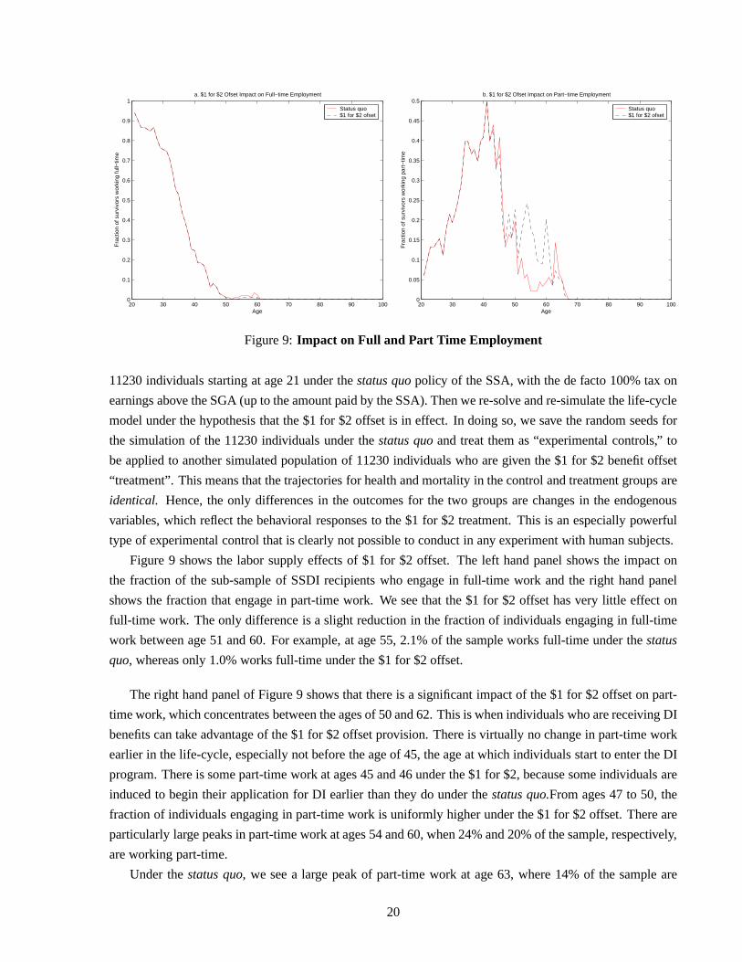
Figure 9 shows the labor supply effects of $1 for $2 offset. The left hand panel shows the impact on

the fraction of the sub-sample of SSDI recipients who engagein full-time work and the right hand panel

shows the fraction that engage in part-time work. We see thatthe $1 for $2 offset has very little effect on

full-time work. The only difference is a slight reduction inthe fraction of individuals engaging in full-time

work between age 51 and 60. For example, at age 55, 2.1% of the sample works full-time under thestatus

quo, whereas only 1.0% works full-time under the $1 for $2 offset.

The right hand panel of Figure 9 shows that there is a significant impact of the $1 for $2 offset on part-

time work, which concentrates between the ages of 50 and 62. This is when individuals who are receiving DI

benefits can take advantage of the $1 for $2 offset provision.There is virtually no change in part-time work

earlier in the life-cycle, especially not before the age of 45, the age at which individuals start to enter the DI

program. There is some part-time work at ages 45 and 46 under the $1 for $2, because some individuals are

induced to begin their application for DI earlier than they do under thestatus quo.From ages 47 to 50, the

fraction of individuals engaging in part-time work is uniformly higher under the $1 for $2 offset. There are

particularly large peaks in part-time work at ages 54 and 60,when 24% and 20% of the sample, respectively,

are working part-time.

Under thestatus quo, we see a large peak of part-time work at age 63, where 14% of the sample are

20

working part-time. The increase in labor force participation after age 62 in thestatus quosimulations reflects

the opportunistic use of the TWP option. The opportunistic use of the TWP increase after age 62 specifically

because after age 62 DI recipients have a fall back option in the form of the SSA early retirement benefits.

This, in turn, helps them shield themselves from the risk that a return to work could trigger a higher chance

of termination due to a CDR. Overall, the fraction of SSDI recipients who choose to return to work at some

point during their DI spell increases from 9.5% under thestatus quo, to 48.9% under the $1 for $2 offset.

Furthermore, those who return to work, also work for more years, namely an average of 2.9 years under the

$1 for $2 offset, but only one year under thestatus quo.This is because under thestatus quoDI recipients

are largely exploiting the trial work provision and do not work beyond it since it would result in termination

from the DI program. In contrast, under the $1 for $2 offset DIrecipients are given larger incentives to enter

a TWP and to continue working after the end of the TWP.

Independent evidence that a $1 for $2 benefit offset providesa strong work incentive is provided in a

study by Muller (1992) that followed 59,000 SSDI beneficiaries who were first entitled to benefits between

age 55 and 64. About 11% of them returned to work at some point after their initial entitlement. Of these,

71% returned to work after age 62, and 47% returned to work after age 65. This is of significant importance,

because SSDI beneficiaries can convert from DI to OA benefits at age 62, and the OA program has a $1 for

$2 offset above a substantially higher disregard level.19 At age 65 the earnings test falls to a $1 for $3 offset

above the higher disregard level. Thus, it is not surprisingthat the majority of SSDI beneficiaries return

to work at ages where the earnings test is less binding. The life-cycle model’s predictions of the timing of

return to work by DI beneficiaries are quite consistent with these findings.

Figure 10 provides the model’s prediction of the other majoreffect of the $1 for $2, namely theinduced

entry effect. The left hand panel depicts the fraction applying for DI benefits, while in the right panel

the fraction on the SSDI rolls is depicted. We see only a modest induced entry effect here. Overall, 134

individuals apply for SSDI, and 95 of those are ultimately awarded SSDI benefits under thestatus quo

simulation, whereas 137 individuals apply, and 98 of them are ultimately awarded SSDI benefits, under the

$1 for $2. Evidently, the net gain in expected discounted utility resulting from the option to work while

receiving DI benefits under the $1 for $2 offset is not large enough to induce people to apply for benefits.

Note that under the $1 for $2 offset the ultimate award rate is71.5%, only slightly higher than 70.9%, under

thestatus quo. That is, applicants who are initially rejected have a slightly stronger incentive to appeal an

initial rejection under the $1 for $2 offset than under thestatus quo.

In the right hand panel of Figure 10 we see that SSDI rolls increase by 3.1% in our simulations, some-

what larger than the 2.2% increase in applications for SSDI.This is caused by the fact that the mean duration

on the DI program increases by.3 years, from 12.7 years under thestatus quoto 13.0 years under the $1

for $2 offset. It one might be tempted to associate this with the fact that DI recipients have less incentive

to leave the rolls under a $1 for $2 offset (i.e.,reduced exit effect). However, the increase in durations is

actually due to a.3 reduction in the mean age of first receipt of DI benefits, which is closely related to the

induced entry effect. At the margin some new disabled individuals who did not apply for DI benefits under

19For example, in 1989 the SGA was $300 per month, but the OA earnings test disregards were $540 and $740 per month, forearly and normal retirees, respectively.

21

40 42 44 46 48 50 52 54 56 58 60 62 640

0.5

1

1.5

2

2.5

3

3.5

4

4.5

5

Age

a. $1 for $2 Ofset Impact on Application for Disability

Fra

ctio

n of

sur

vivo

rs a

pply

ing

for

SS

DI

Status quo$1 for $2 ofset

40 42 44 46 48 50 52 54 56 58 60 62 640

1

2

3

4

5

6

7

8

Age

b. $1 for $2 Ofset Impact on Disability Roles

Per

cent

of s

urvi

vors

Rec

eivi

ng S

SD

I

Status quo$1 for $2 ofset

Figure 10:Impact on SSDI Applications and Rolls

the status quoare induced to apply under the $1 for $2 offset. In addition there are also individuals who

applied in both cases, but are induced to apply slightlyearlier under the $1 for $2 offset. Consequently, the

combined effects of induced entry and the increase in mean duration on the program result in an increase of

5.9% in the number ofperson-yearsspent on SSDI rolls.

The life-cycle model’s prediction of the induced entry effect lies between the projections of the SSA and

CBO. As indicated above, a 1994 study by James McGlaughlin, of the SSA Office of the Actuary, predicted

that the $1 for $2 program would result in 400,000 additionalinduced recipientsover a 10 year period. This

amounts to an approximate 6.4% increase in the annual numberof workers awarded DI benefits, nearly

three times larger than the 2.2% increase predicted by our model.20 The CBO predicts that there would be

75,000 induced filers over the 10 year period considered by McGlaughlin, that is, an increase in SSDI of

approximately 1.2%.

Figure 11 shows the impact of the $1 for $2 offset on Social Security contributions and benefit payments

for the sub-population of SSDI recipients.A priori the effect of the $1 for $2 on net benefit payments is

unclear. Although recipients are on the rolls for a longer period, they are receiving reduced benefits when

they are working due to the $1 for $2 offset. Also, when they are working they are making Social Security

contributions on their wage earnings. The left hand side panel of the figure shows that despite the reduction

in benefits due to increased part-time work under the $1 for $2offset, DI benefit payments are slightly

higher. In particular, between the ages of 50 and 60 DI benefits are 4.3% higher under the $1 for $2 offset

20Projecting the latest data on DI rolls from the 2004 Annual Statistical of the SSA, the 5.86 million adult beneficiaries asofDecember of 2003, will grow to 6.18 million by the end of 2004,assuming the average growth rate of 5.3% in DI rolls overthe period 2001 to 2003 will persist. Thus, McGlaughlin’s study implies an induced entry effect of approximately 6.4% (i.e.,400,000/(6.18 million)). It is not clear whether McGlaughlin’s estimates take account of mortality and conversions ofDI benefitsto OA benefits at the NRA. Our projections do account for thesesources of attrition from the DI program, as well as the CDR’s.Also, McGlaughlin study assumed that the monthly disregardat which the $1 for $2 offset would take effect was $85, substantiallylower than the prevailing SGA level at that point in time of $500. The McGlaughlin report assumed that the amount of inducedentry would not change much if the disregard was increased tothe full SGA level. The life-cycle model predicts that therewouldbe a slightly smaller increase in the rolls, due to induced entry under the lower $85 disregard. The DI rolls is predicted to increaseby 2.1% under the $85 disregard compared to 3.2% under the $500 disregard.

22

20 30 40 50 60 70 80 90 1000

2

4

6

8

10

12

14

Age

a. $1 for $2 Ofset Impact on SSA Benefits

Mea

n va

lue

(in $

000)

for

Coh

ort S

urvi

vors

Status quo$1 for $2 ofset

20 30 40 50 60 70 80 90 1000

0.1

0.2

0.3

0.4

0.5

0.6

0.7

0.8

0.9

1

Age

b. $1 for $2 Ofset Impact on SSA Contributions

Mea

n va

lue

(in $

000)

for

Coh

ort S

urvi

vors

Status quo$1 for $2 ofset

Figure 11:Impact on Social Security Contributions and Benefits

65 700

10

20

30

40

50

60

70

80

Age

a. $1 for $2 Ofset Impact on Age of First Entitlement to OA Benefits

Per

cent

Status quo$1 for $2 ofset

40 45 50 55 600

2

4

6

8

10

12

14

16

18

20

Age

b. $1 for $2 Ofset Impact on Age of First Entitlement to DI Benefits

Per

cent

Status quo$1 for $2 ofset

Figure 12:Impact on Age of Entitlement to OA and DI Benefits

than under thestatus quo.

Figure 12 shows the impact of the $1 for $2 offset on the distributions of ages of first receipt of OA

and DI benefits. Figure 12a shows that there is hardly any effect on the ages of first receipt of OA benefits.

However, we do see a very small increase in claims for OA benefits at age 65 relative to age 62. This, in

turn, contributes to higher benefit payments after age 65 under the $1 for $2 offset. Figure 12b shows there

is a slight downward shift in the ages of first receipt of DI, from 50.6 years under thestatus quoto 50.3 years

under the $1 for $2 offset.

In order to summarize the net impact of the $1 for $2 on the fiscal balance of the SSDI program, we

compute the net present discounted value of SSDI benefits, where both contributions and benefits paid to

the sub-population of SSDI recipients over their lifetimesare discounted at a real interest rate of 2%. We

23

provide a summary of the fiscal implications of the $1 for $2 offset in Table 1. The summary is provided

only for the sub-population of SSDI recipients in the simulation cohort.

Table 1: Summary of the Budgetary Impacts of the $1 for $2 Offset

Item Status Quo $1 for $2 % Changeoffset

Number of DI applicants 134 137 +2.2%Number of DI recipients 95 98 +3.2%Person-years spent on DI 1273 1348 +5.9%Number of DI recipients who returned to work 9 48 +533%Mean Years of Part Time Work on DI 1 2.9 +190%Mean Years of Full Time Work on DI 0 0 0%

Present value of Federal Tax Payments ($000) $1938.92 $ 1872.75 -3.4%Present value of Social Security contributions ($000) $3,003.26 $3,129.84 +4.2%Present value of Social Security benefits ($000) $10,940.08$11,474.07 +4.9%Net Present value of Cost of SSDI beneficiaries ($000) $ 5,997.90 $6,471.48 +7.9%Present value of pre-tax wage earnings ($000) $24,219.80 $25,240.65 +9.3%Present value of consumption ($000) $ 33,116.34 $ 34,684.56 +4.6%

We see that the present value of benefits paid under the $1 for $2 offset increases by about 4.9% from

$10.9 million to $11.5 million. However, on a per beneficiarybasis, the present value of benefits increases

by only 1.6%, from $115,159 to $117,082. That is, while each beneficiary is collecting slightly higher

benefits, due to a longer duration in the program under the $1 for $2 offset, the increase in aggregate benefit

payments is largely due to the induced entry effect. Note also that the present value of Federal tax payments

is slightly lower under the $1 for $2 offset. This is because of the fact that thelow part-time earnings of

many of the DI recipients who return to work qualify them for tax rebates under the EITC program. Overall,

the net present value of the cost of the DI program in our simulations (i.e., the present value of benefits less

the present value of contributions and Federal taxes), increase by 7.9% under the $1 for $2 offset, from $6.0

million to $6.5 million. On a per beneficiary basis, the present value of net costs rise by 4.6%, from $63,147

to $66,041 per beneficiary.

The results suggest that implementation of the $1 for $2 offset policy would result in a modest increase

in DI applications, awards, rolls, and net expected discounted costs. However, the $1 for $2 offset provides

some of the SSDI recipients with clear welfare improvement.The $1 for $2 policy is found to be strictly

welfare enhancing, since it raises the payments (and thus consumption) to SSDI recipients under states

of the world where they experience a recovery, and wish to return to work. On the other hand, these

increase payment do not reduce payments to the SSDI beneficiaries in other states of the world. Indeed,

Table 1 demonstrate that the present value of pre-tax wage earnings increase by 9.3% higher, while that of

consumption increase by 4.6%, under the $1 for $2 offset policy than under thestatus quo.

Figure 13 shows the impact of the $1 for $2 on consumption and wealth accumulation by age. Figure 13a

shows that the average consumption under the $1 for $2 offsetis higher than that understatus quoat every

age. Similarly, Figure 13b demonstrates that net worth is also higher under the $1 for $2 offset at all ages.

24

20 30 40 50 60 70 80 90 1006

7

8

9

10

11

12

13

Age

a. $1 for $2 Ofset Impact on Consumption

Mea

n va

lue

(in $

000)

for

Coh

ort S

urvi

vors

Status quo$1 for $2 ofset

20 30 40 50 60 70 80 90 10012

14

16

18

20

22

24

26

28

Age

b. $1 for $2 Ofset Impact on Wealth Accumulation

Mea

n va

lue

(in $

000)

for

Coh

ort S

urvi

vors

Status quo$1 for $2 ofset

Figure 13:Impact on Consumption and Net Worth

20 30 40 50 60 70 80 90 10095

100

105

110

115

120

Age

Rat

io

Status quo$1 for $2 ofset

Figure 14:Ratio of Consumptions: $1 for $2 Offset vs. Status Quo

Nevertheless, note that there is virtually no increase in consumption and net worth prior to age 45, and

the biggest increases occur between the ages of 55 and 70. It is evident that individuals who return to work

under the $1 for $2 offset, increase their consumption immediately, but they also use a significant fraction

of these earnings to increase their savings for their retirement years, which last well into their 80’s.

Figure 14 plots the ratio of the mean consumption for DI beneficiaries under the $1 for $2 and under the

status quo. We see that there are particular ages at which there are fairly large increases in consumption,

sometimes by more than 18%, under the $1 for $2 offset. Over the entire life-cycle, consumption increases

by an average of 2.2% per year, and by 6.9% per year between ages 45 and 65.

We conclude this section with a summary of the welfare effects of the $1 for $2 offset policy. As we

have emphasized above, the $1 for $2 offset is certainly strictly welfare improving relative to thestatus

quo. Under the $1 for $2 offset policy, those that experience a recovery have the option of continuing

25

20 30 40 50 60 70 80 90−15

−10

−5

0

5

10

Age

a. $1 for $2 Ofset Impact on Expected Discounted Utility

Mea

n va

lue

for

Coh

ort S

urvi

vors

Status quo$1 for $2 ofset

20 30 40 50 60 70 80 90−3.5

−3

−2.5

−2

−1.5

−1

−0.5

0

0.5

1

1.5

Age

b. $1 for $2 Ofset Impact on Current Period Utility

Mea

n va

lue

for

Coh

ort S

urvi

vors

Status quo$1 for $2 ofset

Figure 15:Impact on Expected Discounted and Current Period Utility

to receive reduced SSDI benefits while continue working after the TWP. The simulations of the life cycle

model show that this is an attractive option for nearly 50% ofSSDI beneficiaries, who have experienced

an improvement in their health status, and want to return to part-time work. These individuals are now

receiving a combination of wage earnings and (reduced) SSDIbenefits, rather than not working at all and

relying exclusively on a relatively small SSDI benefits.

Figure 15a plots the mean of the value functionVt(aw,w,h,ss), i.e., the expected discounted utility from

the current age onwards, as a function of age. Figure 15b plots the current period utility functionu(c, l ,h,ss),

as a function of age. Note that bothV andu initially decline with age until about age 45. Then they increase

until leveling off around age 70.

The decline in utility between the ages of 20 and 45 is a resultof the fact that this population started off

healthy when they were in their 20s, but their health declined in their 30s and 40s. Many of these individuals

who became disabled, in these age ranges, were deterred fromapplying for DI benefits by the “hassle costs”.

Consequently, they stopped working and lived off of their savings, hoping for a recovery. As their disability

persisted and their savings dwindled, most of these individuals decided to incur the hassle costs of applying

for DI in their 40s. Once they got onto DI their welfare started to improve since their DI benefits enabled

them to increase their consumption. Also, about 50% of theseindividuals started to experience recoveries

after several years on DI, and this lead to increasing welfare between ages 50 and 75.

Figure 15 indicates that welfare is only slightly higher under the $1 for $2 offset than under thestatus

quo. Indeed the increase in utility and welfare is barely visible in these graphs. There are several reasons for

this finding. First, our welfare calculations account for the disutility of work effort. Thus, while consumption

does rise significantly under the $1 for $2 offset, the rise inconsumption came at a cost of forgone leisure

by individuals who decide to return to work. While individuals are better off from having done so, in an

ex antesense, the disutility of work effort very nearly counterbalances the increased utility from the higher

consumption they could afford as a result of their work effort.

Second, although the $1 for $2 offset is strictly more generous than thestatus quo, it still amounts to a

26

very high 50% surtax on earnings. Furthermore, this surtax applies to individuals with relatively low average

earnings anyway, who are older, face a higher disutility of work, and are not likely to find very lucrative jobs.

The combination of all these factors implies that the $1 for $2 offset is, on average, not a great deal for DI

beneficiaries.

Finally, the utilities in Figure 15 are an average of utilities of 50% of the population of DI beneficiaries

who never experienced a recovery from disability and 50% whodid. For those who never experienced any

recovery, the $1 for $2 offset is not a valuable option. It is always possible that a disabled DI beneficiary

will recover in the future, and thus the $1 for $2 offset has some value, disability is a persistent state, the

value of this option cannot not be very high.

Clearly, the $1 for $2 option is most valuable for DI beneficiaries who have recovered from their disabil-

ities. However, when we compute the increase in welfare due to the $1 for $2 offset for a younger person

who has not yet become disabled, or considered applying to the DI program, the increase inex antewelfare

is negligible. The increase in welfare due to the $1 for $2 becomes significant only when a person gets into

their middle ages and becomes disabled. The welfare gain is highest for those who are already on DI and

who have recovered from their disability.

The analysis of welfare changes is the key to understanding why our model predicts small induced entry

effect. Theex antegains facing a prospective SSDI applicant are not large whenone factors in: (1) the

chance that after incurring the hassle of submitting an application it would ultimately be rejected; (2) the

chance that once on the program the person would actually experience a medical recovery that would make

it possible to work; and (3) the high effective 50% surtax on the benefits for SSDI beneficiaries who do

return to work. The combination of all these factors impliesthat the net gain from the $1 for $2 from an

ex ante point of view is small. Unless the “gradient” in the hassle costs for those who are at the margin

of indifference between applying and not applying for SSDI benefits is very flat, the small increase in net

expected discounted utility from the $1 for $2 offset will not result in a large amount of induced entry.

4 Conclusions and Discussion

This paper examines the impact of a new disability policy that has been considered recently by the Social

Security Administration (SSA), namely the $1 for $2 benefit offset. We use a numerically solved life-cycle

model, and show that it can be an extremely useful tool for Social Security policy evaluation and forecasting,

particularly for examining the proposed reform of the SSDI program. The SSA was initially mandated to

evaluate this policy change using a large scale demonstration project. The key issue that motivated the

U.S. Congress to obligate the SSA to undertake a costly, time-consuming demonstration project, is the

concern aboutinduced entry. The key question that has been raised is: Would the $1 for $2 offset be

considered a significant increase in the generosity of the SSDI program by potential DI applicants resulting

in large increases in applications, awards, and program costs?

Our analysis has provided a number of new insights into how entering the DI roll and return to work

incentives might be affected by the way the SSDI program is being administered. Specifically, the life-

cycle model indicates that individuals are very sensitive to the SSA’s policy regarding continuing disability

27

reviews (CDRs). If DI recipients believe that taking advantage of the $1 for $2 offset will result in them

being a target for higher rates of CDRs in the future, then a significantly lower number of DI recipients will

return to work and, in turn, the induced entry effect becomesnegligible. We also demonstrate the usefulness

of the life-cycle model in providing accurate predictions for the possible impact of the $1 for $2 benefit

offset proposal that has been considered recently by the SSA. In particular, the model is able to accurately

predict individuals’ observed responses in the Health and Retirement Study regarding: (1) health status;

(2) employment decisions; (3) age of first receipt of DI and OAbenefits; (4) wealth; and (5) wages. Since

these are the most important factors affecting the application decisions for DI benefits, and/or are the most

obvious outcomes of such decision, it makes one comfortableusing it for the purpose of evaluating the

proposed $1 for $2 benefit offset policy.

Careful examination of the various simulations provided inthe paper indicates that the cost of the newly

suggested policy is not huge. Moreover it provides some of the people with very strong incentives to return

to work, even if in many cases it is only to part-time jobs. Theinduced entry effect that Congress and

the SSA are very concerned about seems to be quite small. Thisis mainly because the proposed policy

provides a welfare enhancement tool only for people who found themselves disabled at some point of their

career. From an ex-ante point of view, the proposed plan doesnot give people enough incentives to apply for

disability benefits. However, once a person finds himself on the DI rolls, it gives him/her ex-post incentives

to get of them. Consequently, the overall net increase in costs of the SSDI program are relatively small.

It is clear from our results that the $1 for $2 offset proposalwould benefit those currently receiving

disability benefits, however, does not necessarily have thepositive fiscal effects the government agencies

would be hoping for. If the policy objective is to try to integrate disabled workers into the labor force at a

reasonable cost, this could be a good policy, given the relatively small induced entry effectswe predict. If

the objective is to reduce the overall cost of the system by allowing disabled individuals to come back to

work so that they eventually get off the rolls, then this might not be the ideal policy to put in place.

There is, however, a different way of thinking about this proposed reform that can illuminate the policy

debate, and it is as an example of how to essentially change the current disability system from one that only

offers benefits to those completely disabled, to one, that for all purposes, offers partial benefits. The appeal of

this proposal to accomplish the latter objective is that it allows individuals to self-select themselves into their

own disability level (defined here by their benefit level withrespect to someone that receives full benefits),

without imposing particular ex-ante thresholds, like in countries were partial benefits are the norm, such as

Germany, Sweden, or Spain. An alternative reform of the system might be to actually offer partial benefits.

However, that is likely to come at a higher administrative cost, and would still leave open the handling of

the millions currently on the rolls.21 Given that the dichotomous nature of disability in the United States is

possibly imposing a high welfare cost on those partially disabled, our results can be understood as an initial

measure of the gains of moving towards ade factosystem of partial benefits, which would allow individuals

to adjust their dependence from the system to their ability to exert productive work in the market.

The empirical life-cycle model we have developed is a prime example for the non-experimental alterna-

tives that have been advocated by Tuma (2001) and Moffitt (2003), as a necessary alternative to randomized

21With the exemption of the current efforts by Yin (2005), which has help us understand our contribution to the policy debatebetter, there is currently almost no research on this topic regarding the U.S. system.

28

experiments. Indeed, the approach used here may be one of a few alternatives at our disposal when it comes

to the evaluation of program entry effects. The calibrated model we have used here to forecast the induced

entry effects associated with the $1 for $2 offset delivers detailed and credible predictions about the impli-

cation of the proposed policy. In fact, we are not aware of anyother alternative modeling approach that is

capable of generating predictions that would be more detailed and accurate than the approach we used here.

While we make no claim that randomized experiments are not useful, we do argue that they are not

sufficient, and in many cases are not feasible. When randomized experiments are not feasible, the most

obvious alternative is the approach we have adopted here, not simply introducing new policies without any

pretesting. This is particularly true when it comes to something as important as Social Security, since many

people are crucially dependent on these benefits. While somepolicy changes are inevitable, it is better, in

general, to have fewer well thought out policy changes than to have many semi-experimental or haphazardly

chosen ones.

We have argued throughout this paper that the life-cycle models are sufficiently realistic to provide

credible predictions of a wide range of policy changes, but we also argue that there is a very important

complementarity between survey data collection, randomized experiments, and econometric modeling. We

believe that the government should be investing in all threeareas, and that these “R&D expenditures” will

have a very high long term payoff in enabling the government to develop more cost-effective policies,

particularly with respect to welfare and Social Security.22However, we strongly believe that model building

is the most inexpensive investment that can be made to improve the nation’s analytical capabilities. It will

then be up to researchers at government institutions, and policy makers, to decide whether these models

provide useful tools in their decision making process.

It is still an open question whether any of these models will actually be used in practice as inputs to policy

making. However, some government agencies, particularly the Congressional Budget Office, are already

using life-cycle models for their long term forecasting. Itseems likely that inter-agency competition will

ultimately lead to the adoption of better analytical tools,and hopefully greater investment in data collection

and (controlled) experimentation.

22A good illustration for this complementarity is provided ina recent study by Todd and Wolpin (2003), which uses data froma large scale randomized experiment in Mexico (known as PROGRESA), and panel data on the families under study well beyondthe duration of the policy, to determine whether subsidies to parents who keep their children in school will significantly improveeducational outcomes.

29

5 References

Benı́tez-Silva, H., Buchinsky, M., Chan, H. Cheidvasser, S. and J. Rust (1999): “An Empirical Analysis of

the Social Security Disability Application, Appeal and Award Process”Labour Economics, 6, 147–

178.

Benı́tez-Silva, H. Buchinsky, M. and J. Rust (2004): “How Large is the Bias in Self-Reported Disability?”

Journal of Applied Econometrics, 19-6649–670.

Benı́tez-Silva, H. Buchinsky, M. and J. Rust (2005): “How Large are the Classification Errors in the Social

Security Disability Award Process?” manuscript, University of Maryland.

Benı́tez-Silva, H., and F. Heiland (2004): “Early Claimingof Social Security Benefits and Labor Supply

Behavior of Older Americans,” manuscript, SUNY-Stony Brook.

Bernheim, D., Skinner, J., and S. Weinberg (2001): “What Accounts for the Variation in Retirement Wealth

Among U.S. Households?”American Economic Review, 91-4, 832–857.

Congressional Budget Office (1997): “Time-Limiting Federal Disability Benefits,” Memorandum. Wash-

ington D.C.

Engen, E., Gale, W.G., and C.E. Uccello (1999): “The Adequacy of Household Saving,”Brookings Papers

on Economic Activity, 2, 65–165.

French, E. (2001): “The Effects of Health, Wealth, and Wageson Labor Supply and Retirement Behavior,”

forthcoming in theReview of Economic Studies.

Moffitt, R. (2003): “The Role of Randomized Field Trials in Social Science Research: A Perspective from

Evaluations of Reforms of Social Welfare Programs” manuscript, Department of Economics, Johns

Hopkins University.

Muller, L.S. (1992): “Disability Beneficiaries Who Work andTheir Experience Under Program Work

Incentives”Social Security Bulletin, 55-2, 2–19.

Muller, L.S. (2000): “The Search for Evidence of a Labor Supply Response to a Benefit Offset” Office of

Research, Evaluation and Statistics, Social Security Administration.

Muller, L.S., Scott, G., and B.V. Bye (1996): “Work and Earnings of SSI Disability Recipients”Social

Security Bulletin59-222–42.

Nagi, S.Z. (1969): Disability and Rehabilitation: Legal, Clinical, and Self-Concepts and Measurement,

Ohio State University Press.

Neumark, D. and E.T. Powers (2003): “The Effects of Changes in State SSI Supplements on Pre-

Retirement Labor Supply” NBER working paper 9851.

30

Rust, J. and C. Phelan (1997): “How Social Security and Medicare Affect Retirement Behavior in a World

of Incomplete Markets,”Econometrica, 64-5, 781–832.

Scholz, J.K., A. Seshadri, and S. Kitatrakun (2006): “Are American Saving ‘Optimally’ for Retirement?”

Journal of Political Economy, 114-4, 607–643.

Todd, P. and K. Wolpin (2003): “Using a Social Experiment to Validate a Dynamic Behavioral Model

of Child Schooling and Fertility: Assessing the Impact of the School Subsidy Program in Mexico,”

manuscript, University of Pennsylvania.

Tuma, N. (2001): “Approaches to Evaluating Induced Entry into a New SSDI Program with a $1 Reduction

in Benefits for each $2 in Earnings,” manuscript, Stanford University.

van der Klaauw, W., and K.I. Wolpin (2002): “Social Security, Pensions and the Savings and Retirement

Behavior of Households,” manuscript, University of North-Carolina-Chapel Hill.

Wheeler, P.M. (1996): “Message from the Associate Commissioner,”Social Security Bulletin, 59-1, p. 2.

Yin, N. (2005): “Partial Benefits in the Social Security Disability Insurance: A Policy Alternative,”

manuscript, SUNY-Stony Brook.

31