Industrial Internship Robin Verschueren - syscop · Industrial Internship Robin Verschueren Authors...

Industrial Internship

Robin Verschueren

Authors Robin VerschuerenDate November 15, 2013Version FinalConfidentiality Confidential

Industrial Internship Report - Confidential November 15, 2013

Contents

Preliminaries 3

1 Introduction: LMS, a Siemens Business 41.1 The birth and growth of LMS . . . . . . . . . . . . . . . . . . . . . . . . . . . . . . . . 41.2 Activities . . . . . . . . . . . . . . . . . . . . . . . . . . . . . . . . . . . . . . . . . . . . 4

1.2.1 Testing . . . . . . . . . . . . . . . . . . . . . . . . . . . . . . . . . . . . . . . . 41.2.2 Mechatronic simulation . . . . . . . . . . . . . . . . . . . . . . . . . . . . . . . 41.2.3 Engineering services . . . . . . . . . . . . . . . . . . . . . . . . . . . . . . . . . 5

2 The internship 52.1 Task Description . . . . . . . . . . . . . . . . . . . . . . . . . . . . . . . . . . . . . . . 52.2 Role in company activities . . . . . . . . . . . . . . . . . . . . . . . . . . . . . . . . . . 52.3 The setup . . . . . . . . . . . . . . . . . . . . . . . . . . . . . . . . . . . . . . . . . . . 52.4 The project: planning . . . . . . . . . . . . . . . . . . . . . . . . . . . . . . . . . . . . . 62.5 The project: towards Milestone 1 . . . . . . . . . . . . . . . . . . . . . . . . . . . . . . 7

2.5.1 Camera calibration . . . . . . . . . . . . . . . . . . . . . . . . . . . . . . . . . . 72.5.2 Kalman filter . . . . . . . . . . . . . . . . . . . . . . . . . . . . . . . . . . . . . 82.5.3 The communication between VPU and VCU . . . . . . . . . . . . . . . . . . . . 102.5.4 The communication between VCU and RC controller . . . . . . . . . . . . . . . 102.5.5 The Vehicle Control Unit . . . . . . . . . . . . . . . . . . . . . . . . . . . . . . . 112.5.6 The integration and Milestone 1 . . . . . . . . . . . . . . . . . . . . . . . . . . . 11

2.6 The project: towards Milestone 2 . . . . . . . . . . . . . . . . . . . . . . . . . . . . . . 122.6.1 Integration with Simulink . . . . . . . . . . . . . . . . . . . . . . . . . . . . . . . 122.6.2 Measuring the control actions . . . . . . . . . . . . . . . . . . . . . . . . . . . . 122.6.3 Identifying a car model . . . . . . . . . . . . . . . . . . . . . . . . . . . . . . . . 152.6.4 PID control on the final track . . . . . . . . . . . . . . . . . . . . . . . . . . . . 16

2.7 The project: towards Milestone 3 . . . . . . . . . . . . . . . . . . . . . . . . . . . . . . 182.7.1 Problem formulation . . . . . . . . . . . . . . . . . . . . . . . . . . . . . . . . . 182.7.2 Implementation . . . . . . . . . . . . . . . . . . . . . . . . . . . . . . . . . . . . 202.7.3 Trajectory Tracking: results . . . . . . . . . . . . . . . . . . . . . . . . . . . . . 202.7.4 Trajectory planning . . . . . . . . . . . . . . . . . . . . . . . . . . . . . . . . . . 21

3 Conclusion 21

4 Link with university programme 22

5 Logbook 22

6 Appendix A: Technical details of the setup 24

7 Appendix B: from states to error states 24

Robin Verschueren Page 2 of 25


Preliminaries

Student: Robin Verschueren (2nd Master Wiskundige Ingenieurstechnieken)

Company: LMS,Interleuvenlaan 68, Researchpark Haasrode Z1, 3001 Leuven

Company contact: Stijn De Bruyne

Supervisor: Karl Meerbergen

Period: July 22nd until August 30th



1 Introduction: LMS, a Siemens Business

1.1 The birth and growth of LMS

LMS was founded in 1980 as a spin-off of the KU Leuven. Initially LMS only offered testing asa service, but later also the development of testing software started. More recently, in the mid-1990s, simulation software was added to the product portfolio of LMS. Through time LMS acquiredseveral companies to make these developments possible. For example, recently (25 Aug 2011),LMS acquired a 60% controlling majority position of SAMTECH, the Liege-based European providerof Computer Aided Engineering (CAE) and structure analysis software. More recently still, at theend of 2012, the German holding Siemens acquired LMS as the ’Test and Simulation’ component ofSiemens PLM (Product Lifecycle Management)[3].LMS currently offers the following unique combination of products and services:

• testing systems,

• mechatronic simulation software,

• engineering services.

LMS has become a profitable company, operating in over 30 key locations with about 1200 employeesworldwide. In 2011 the company achieved a turnover of about e160 million [2]. LMS has grown tobecome a worldwide leader in engineering innovation. With multi-domain and mechatronic simulationsolutions, LMS addresses the complex engineering challenges associated with intelligent systemdesign and model-based systems engineering. They have become the partner of choice of more than5000 manufacturing companies worldwide, spread over the automotive, aerospace and mechanicalindustry segments.

1.2 Activities

The leading partner in testing and mechatronic simulation in the automotive, aerospace and otheradvanced manufacturing industries, helps customers get better products to market faster.

1.2.1 Testing

LMS has pioneered many innovative techniques in high-end structural and NVH (noise, vibration &harshness) testing over the years. The full portfolio of LMS testing solutions includes transfer pathanalysis, rotating machinery, structural and acoustics testing, environmental testing, vibration control,report and data management. On the hardware side, the LMS SCADAS family ranges from compactmobile units, autonomous smart recorders, dedicated durability solutions up to high-channel countlaboratory systems.

1.2.2 Mechatronic simulation

Over the last decade, LMS has developed an integrated hybrid process solution simulation, enhancedby test. With LMS mechatronic simulation software and solutions, critical functional performanceattributes are simulated and designed upfront in the development process. This process has enabledLMS customers to slash development times by 30-50%. This is not only a tremendous advantage interms of faster time to market, it also significantly reduced risks and costs. Today, LMS tries to takesimulation a step further, and focuses on energy management and emission reduction, as well as the



almost exponential explosion of electronics and controls in a variety of products, such as intelligentvehicles.

1.2.3 Engineering services

The engineering service team knows how to support all aspects of the development process, fromconceptual design over detailed component development to test-based product refinement and validation.LMS Engineers master a variety of complex domains: noise and vibration, strength and durability,safety and crash, kinematics and dynamics, vehicle handling, eco-engineering and mechatronicsimulation. The LMS Engineering Services centers in Europe, the USA and Asia combine state-of-the-art testing facilities with an extensive simulation infrastructure.

2 The internship

2.1 Task Description

The goal of the industrial internship is to create a setup with automated model race cars (scale 1:43)driving on a race track for demonstrating purposes towards potential customers in the automotivesector. Ultimately, a model based controller will be conceived, performing both the planning andtracking of the race car trajectory.The very first task was to get familiar with the hard/software in place, as well as debugging the VisionProcessing Unit (VPU). Next, a simple proportional controller was developed and tested on the trackto validate the successful integration of the different elements in the closed loop control system. Anessential step on the way to a model based controller is the identification of the vehicle model. Inorder to do this, existing vehicle models were examined, and experiments were carried out in orderto identify the parameters of the model. Finally, a Model Predictive Controller (MPC) for tracking areference trajectory was implemented and experimentally validated on the race track.

2.2 Role in company activities

The last few years, Advanced Driver Assistance Systems (ADAS) have been introduced in passengercars, eg. semi-automated parking and pre-crash systems. The next step would be autonomouslydriving cars, which will be achieved not so far in the future. The internship is a part of the engineeringservices activities of the company that focus on the usage of model-based control techniques forcontrol applications in the next-generation vehicles.

2.3 The setup

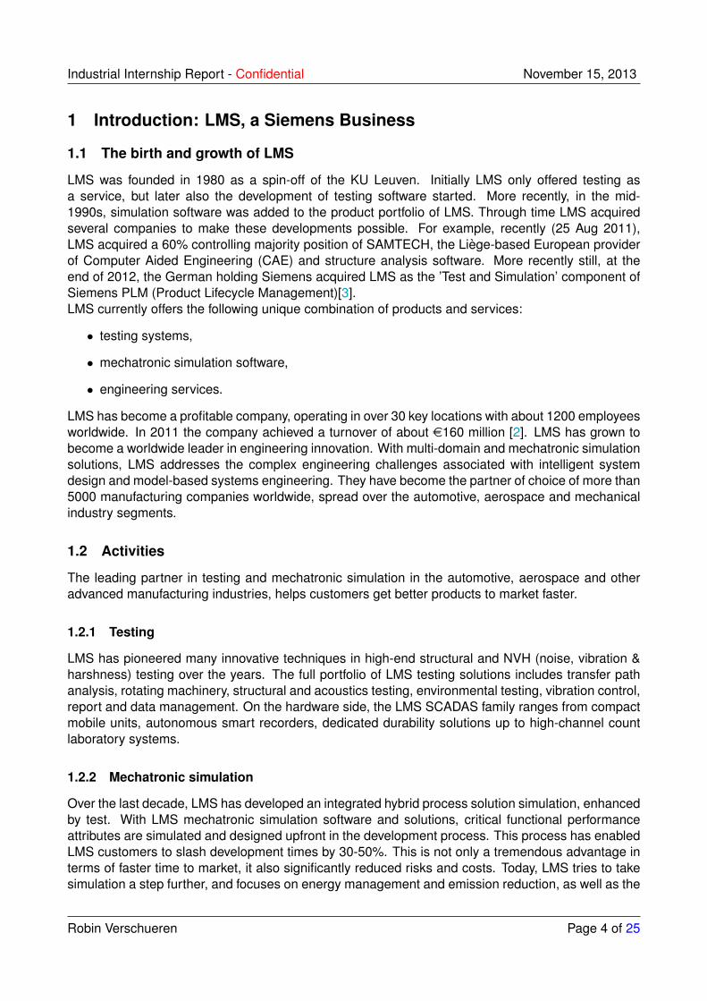
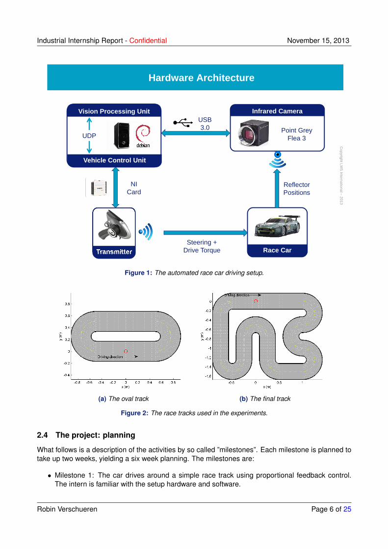
Small scale radio controlled cars (RC-cars) really came of age with the introduction of the KyoshodNaNo model race cars in 2008. These cars will be driven automatically around a track, controlled bya computer, via a data acquisition card (DAQ) which drives the Kyosho RC-controller. The feedbackin terms of the position of the cars will be provided by an infrared camera, which senses the reflectionof some small markers placed on the race cars and sends these images to the computer. The entirearchitecture is shown in Fig. 1. More technical details can be found in appendix A.In the internship, two different tracks were used. The first is a simple oval track (Fig. 2a), the other isa more sophisticated and bigger track, with a chicane, a U-turn and a longer straight section to gainspeed (Fig. 2b). We will call this the final track.


Industrial Internship Report - Confidential November 15, 2013C

opyright LMS

International –2013

4

Hardware Architecture

USB 3.0

Vision Processing Unit

UDP

Infrared Camera

Point Grey Flea 3

Vehicle Control Unit

NI Card

Transmitter Race CarSteering +

Drive Torque

ReflectorPositions

Figure 1: The automated race car driving setup.

(a) The oval track (b) The final track

Figure 2: The race tracks used in the experiments.

2.4 The project: planning

What follows is a description of the activities by so called ”milestones”. Each milestone is planned totake up two weeks, yielding a six week planning. The milestones are:

• Milestone 1: The car drives around a simple race track using proportional feedback control.The intern is familiar with the setup hardware and software.



• Milestone 2: Integration with Simulink. The car drives around a more difficult race track, stillusing proportional control. An appropriate vehicle model is identified.

• Milestone 3: Design of an MPC controller for the tracking of a predefined trajectory.

2.5 The project: towards Milestone 1

At the start of the internship, the following components of the setup were not fully functional:

• Camera calibration

• Kalman filter

• The communication between the Vision Processing Unit (VPU) and the Vehicle Control Unit(VCU)

• The communication between the VCU and the Kyosho RC-controller

These components were fixed during the first two weeks of the internship. While proceeding towardsmilestones 2 and 3, existing components were improved and new components were added.

2.5.1 Camera calibration

The calibration of the camera is crucial for an accurate vision system. It aligns the 3D real worldwith the 2D internal images. As a model for our camera, we use a pinhole model. The calibrationof the camera consists of two steps: an intrinsic calibration and an extrinsic calibration. The intrinsiccalibration deals with the camera distortions, the extrinsic calibration makes sure that the coordinatesystem of the camera is aligned with the world coordinate system. A detailed description on pinholemodels and camera calibration can be found in [4].

Intrinsic calibration Intrinsic calibration of a camera deals with distortions. The distortion of thecamera can be split in two parts: linear distortion and nonlinear distortion. For the linear distortion,the parameters that need to be identified are in the so called camera matrix:xy

w

=

fx 0 cx0 fy cy0 0 1

XYZ

, (1)

where X, Y and Z are the world coordinates, x and y are the camera coordinates. The presenceof w is because of the use of a homography coordinate system (thoroughly explained in [5]). Theunknown parameters to identify are fx, fy (camera focal lengths for each direction) and cx, cy (theoptical center expressed in pixel coordinates).The nonlinear distortion by the camera comes mainly from the ”barrel effect”, or ”fish-eye effect”, asshown in Fig. 3. These distortions can be corrected as follows:

xcorrected = x(1 + k1r2 + k2r

4) (2)

ycorrected = y(1 + k1r2 + k2r

4) (3)

For the computation of both the linear and nonlinear distortion coefficients, we use C++ code providedby ETH in Zurich. It is based on the OpenCV code that can be found at [5], and uses the checkerboard



(a) Distorted. Note the nonlinear barrel effect. (b) Undistorted.

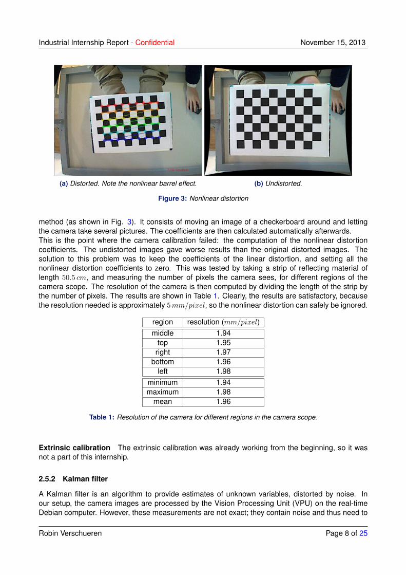
Figure 3: Nonlinear distortion

method (as shown in Fig. 3). It consists of moving an image of a checkerboard around and lettingthe camera take several pictures. The coefficients are then calculated automatically afterwards.This is the point where the camera calibration failed: the computation of the nonlinear distortioncoefficients. The undistorted images gave worse results than the original distorted images. Thesolution to this problem was to keep the coefficients of the linear distortion, and setting all thenonlinear distortion coefficients to zero. This was tested by taking a strip of reflecting material oflength 50.5 cm, and measuring the number of pixels the camera sees, for different regions of thecamera scope. The resolution of the camera is then computed by dividing the length of the strip bythe number of pixels. The results are shown in Table 1. Clearly, the results are satisfactory, becausethe resolution needed is approximately 5mm/pixel, so the nonlinear distortion can safely be ignored.

region resolution (mm/pixel)middle 1.94

top 1.95right 1.97

bottom 1.96left 1.98

minimum 1.94maximum 1.98

mean 1.96

Table 1: Resolution of the camera for different regions in the camera scope.

Extrinsic calibration The extrinsic calibration was already working from the beginning, so it wasnot a part of this internship.

2.5.2 Kalman filter

A Kalman filter is an algorithm to provide estimates of unknown variables, distorted by noise. Inour setup, the camera images are processed by the Vision Processing Unit (VPU) on the real-timeDebian computer. However, these measurements are not exact; they contain noise and thus need to



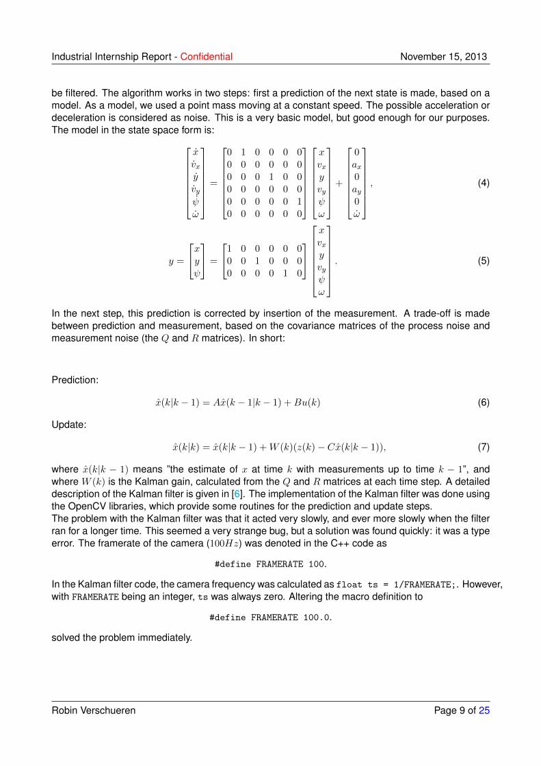
be filtered. The algorithm works in two steps: first a prediction of the next state is made, based on amodel. As a model, we used a point mass moving at a constant speed. The possible acceleration ordeceleration is considered as noise. This is a very basic model, but good enough for our purposes.The model in the state space form is:

xvxyvyψω

=

0 1 0 0 0 00 0 0 0 0 00 0 0 1 0 00 0 0 0 0 00 0 0 0 0 10 0 0 0 0 0

xvxyvyψω

+

0ax0ay0ω

, (4)

y =

xyψ

=

1 0 0 0 0 00 0 1 0 0 00 0 0 0 1 0

xvxyvyψω

. (5)

In the next step, this prediction is corrected by insertion of the measurement. A trade-off is madebetween prediction and measurement, based on the covariance matrices of the process noise andmeasurement noise (the Q and R matrices). In short:

Prediction:

x(k|k − 1) = Ax(k − 1|k − 1) +Bu(k) (6)

Update:

x(k|k) = x(k|k − 1) +W (k)(z(k)− Cx(k|k − 1)), (7)

where x(k|k − 1) means ”the estimate of x at time k with measurements up to time k − 1”, andwhere W (k) is the Kalman gain, calculated from the Q and R matrices at each time step. A detaileddescription of the Kalman filter is given in [6]. The implementation of the Kalman filter was done usingthe OpenCV libraries, which provide some routines for the prediction and update steps.The problem with the Kalman filter was that it acted very slowly, and ever more slowly when the filterran for a longer time. This seemed a very strange bug, but a solution was found quickly: it was a typeerror. The framerate of the camera (100Hz) was denoted in the C++ code as

#define FRAMERATE 100.

In the Kalman filter code, the camera frequency was calculated as float ts = 1/FRAMERATE;. However,with FRAMERATE being an integer, ts was always zero. Altering the macro definition to

#define FRAMERATE 100.0.

solved the problem immediately.



2.5.3 The communication between VPU and VCU

The camera images processed by the Vision Processing Unit (VPU) need to be sent to the VehicleControl Unit (VCU), so it can take the appropriate actions for steering the race car. For this, the UDPprotocol is used. Whenever a camera image is processed by the VPU, the useful information for theVCU (car position: x and y, orientation: ψ, speed: vx and vy and rotational speed: ω) is wrapped in aUDP packet and sent through a local loopback to the VCU (using the IP address 127.0.0.0), which isjust another application running on the same computer as the VPU.The <arpa/inet.h> and the <netinet/in.h> libraries from the Free Software Foundation provide aneasy and well-documented interface for the sending and receiving of UDP and TCP packets. Withthese libraries, the communication was quickly up and running. The low-level code which sends andreceives the actual packets was neatly wrapped in two self written classes UDPclient and UDPserver.The timing of the UDP packets is important: if a packet has a large delay, the information enclosedin it is not up to date, which is detrimental for real-time applications. The timing was tested at thereceiving end (the VCU), the results are shown in Fig. 4. Notice that except for the first packet, allpackets arrive approximately after 0.01 s, which is the sampling speed of the VPU.

0 200 400 600 800 1000 1200 14000

0.02

0.04

0.06

0.08

0.1

0.12

# packets received

time

betw

een

to p

acke

ts (

s)

Figure 4: Time between two UDP packets received by the Vehicle Control Unit.

2.5.4 The communication between VCU and RC controller

Lastly, the (modified) RC controller had to be addressed from within the VCU. The setup is as follows:the VCU drives the National Instruments Data Acquisition Card (DAQ), and the DAQ overrides themanual controls on the Kyosho RC controller. For this, the free and open source library for devicedrivers comedi was used. At first, the wiring plan of the DAQ had to be examined, and the outputvoltages had to be measured. The comedi library provides routines to switch between voltagesand raw data processed by the computer (which takes all integers between 0 and 65535). With amultimeter, the output voltages were assessed to be correct.The RC controller was modified (this work was finished before the start of the internship) to make itpossible to override the signals from the manual controls (the throttle and the steering wheel). Twomini-jack connectors are connected to the central integrated circuit board of the controller: one for



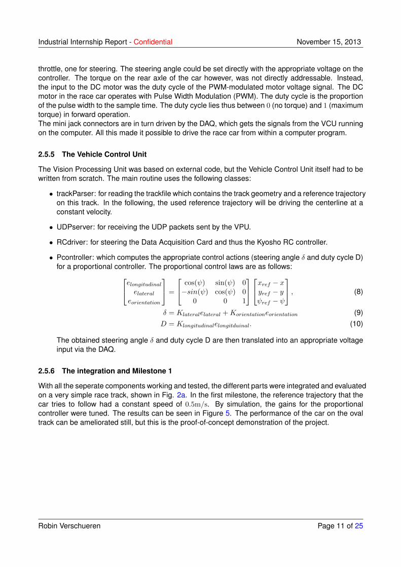
throttle, one for steering. The steering angle could be set directly with the appropriate voltage on thecontroller. The torque on the rear axle of the car however, was not directly addressable. Instead,the input to the DC motor was the duty cycle of the PWM-modulated motor voltage signal. The DCmotor in the race car operates with Pulse Width Modulation (PWM). The duty cycle is the proportionof the pulse width to the sample time. The duty cycle lies thus between 0 (no torque) and 1 (maximumtorque) in forward operation.The mini jack connectors are in turn driven by the DAQ, which gets the signals from the VCU runningon the computer. All this made it possible to drive the race car from within a computer program.

2.5.5 The Vehicle Control Unit

The Vision Processing Unit was based on external code, but the Vehicle Control Unit itself had to bewritten from scratch. The main routine uses the following classes:

• trackParser: for reading the trackfile which contains the track geometry and a reference trajectoryon this track. In the following, the used reference trajectory will be driving the centerline at aconstant velocity.

• UDPserver: for receiving the UDP packets sent by the VPU.

• RCdriver: for steering the Data Acquisition Card and thus the Kyosho RC controller.

• Pcontroller: which computes the appropriate control actions (steering angle δ and duty cycle D)for a proportional controller. The proportional control laws are as follows:elongitudinalelateral

eorientation

=

cos(ψ) sin(ψ) 0−sin(ψ) cos(ψ) 0

0 0 1

xref − xyref − yψref − ψ

, (8)

δ = Klateralelateral +Korientationeorientation (9)D = Klongitudinalelongitduinal. (10)

The obtained steering angle δ and duty cycle D are then translated into an appropriate voltageinput via the DAQ.

2.5.6 The integration and Milestone 1

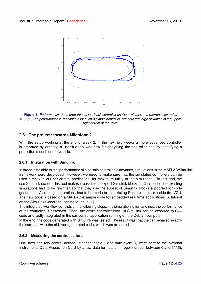
With all the seperate components working and tested, the different parts were integrated and evaluatedon a very simple race track, shown in Fig. 2a. In the first milestone, the reference trajectory that thecar tries to follow had a constant speed of 0.5m/s. By simulation, the gains for the proportionalcontroller were tuned. The results can be seen in Figure 5. The performance of the car on the ovaltrack can be ameliorated still, but this is the proof-of-concept demonstration of the project.



−0.8 −0.6 −0.4 −0.2 0 0.2 0.4 0.6 0.8

−0.4

−0.2

0

0.2

0.4

0.6

0.8

x (m)

y (m

)

Figure 5: Performance of the proportional feedback controller on the oval track at a reference speed of0.5m/s. The performance is reasonable for such a simple controller, but note the large deviation in the upper

right corner of the track.


With the setup working at the end of week 2, in the next two weeks a more advanced controlleris prepared by creating a user-friendly workflow for designing the controller and by identifying aprediction model for the vehicle.

2.6.1 Integration with Simulink

In order to be able to test performance of a certain controller in advance, simulations in the MATLAB/Simulinkframework were developed. However, we need to make sure that the simulated controllers can beused directly in our car control application, for maximum utility of the simulation. To this end, weuse Simulink coder. This tool makes it possible to export Simulink blocks to C++ code. The existingsimulations had to be rewritten so that they use the subset of Simulink blocks supported for codegeneration. Also, major alterations had to be made to the existing Pcontroller class inside the VCU.The new code is based on a MATLAB example code for embedded real time applications. A tutorialon the Simulink Coder tool can be found in [7].The integrated workflow consists of the following steps: the simulation is run and next the performanceof the controller is assessed. Then, the entire controller block in Simulink can be exported to C++code and lastly integrated in the car control application running on the Debian computer.In the end, the code generated with Simulink was tested. The result was that the car behaved exactlythe same as with the old, non-generated code, which was expected.

2.6.2 Measuring the control actions

Until now, the two control actions (steering angle δ and duty cycle D) were sent to the NationalInstruments Data Acquisition Card by a raw data format: an integer number between 0 and 65535.



However, we would like to know the exact relation between voltages and actual control actions.Therefore, two experiments have been carried out.

1. The steering angle: there is a very simple relation between steering angle and radius ofcurvature of the curve driven by a car. It is given by

radius =track

2+

wheelbasesin(δ)

, (11)

where track and wheelbase of a car are defined as in Fig. 6. By By sending a fixed voltage tothe steering system, the car will drive circles. By measuring the radius of these circles, a mapfrom steering angle to voltage can be made using a linear least squares fit. The results areshown in Fig. 7.

Figure 6: Definition of track and wheelbase of a car.

Figure 7: Relation between the voltage applied to the RC controller and the steering angle of the car. Themeasurements are shown in blue, the least-squares curve is shown in red.

2. The duty cycle. To measure the duty cycle-to-voltage mapping, we used a digital oscilloscope.By turning up the voltage applied to the handheld controller, the duty cycle becomes larger and



larger. The duty cycle can be read off the oscilloscope by fixing the screen so that it containsone period of the motor sample time. The proportion of the time that the voltage is high (for theused DC motor, a high voltage corresponds to 2V ) is the duty cycle The measured values canbe found in Table 2. Note that a low voltage corresponds to a high duty cycle. We also foundthat the duty cycle changes in a discrete way, the changing points are shown in the table. InFig. 8, the measurements are plotted along with a linear fit. The duty cycle-to-voltage mappingis obtained by inverting the red curve in the figure.

Voltage (V ) pulse width (µs) dutycyle (-)1.39 14 0.071.35 31 0.141.31 47 0.231.28 63 0.301.24 79 0.381.20 95 0.461.17 111 0.531.12 127 0.611.09 143 0.691.05 163 0.781.01 176 0.850.98 193 0.930.93 208 1.00

Table 2: Measurements of the voltage applied to the RC controller and the corresponding duty cycle appliedto the DC motor.

0.9 1 1.1 1.2 1.3 1.4 1.50

0.1

0.2

0.3

0.4

0.5

0.6

0.7

0.8

0.9

1

voltage (V)

duty

cycl

e (−

)

Figure 8: Mapping of the voltage to the duty cycle. In red, a linear fit is shown.



2.6.3 Identifying a car model

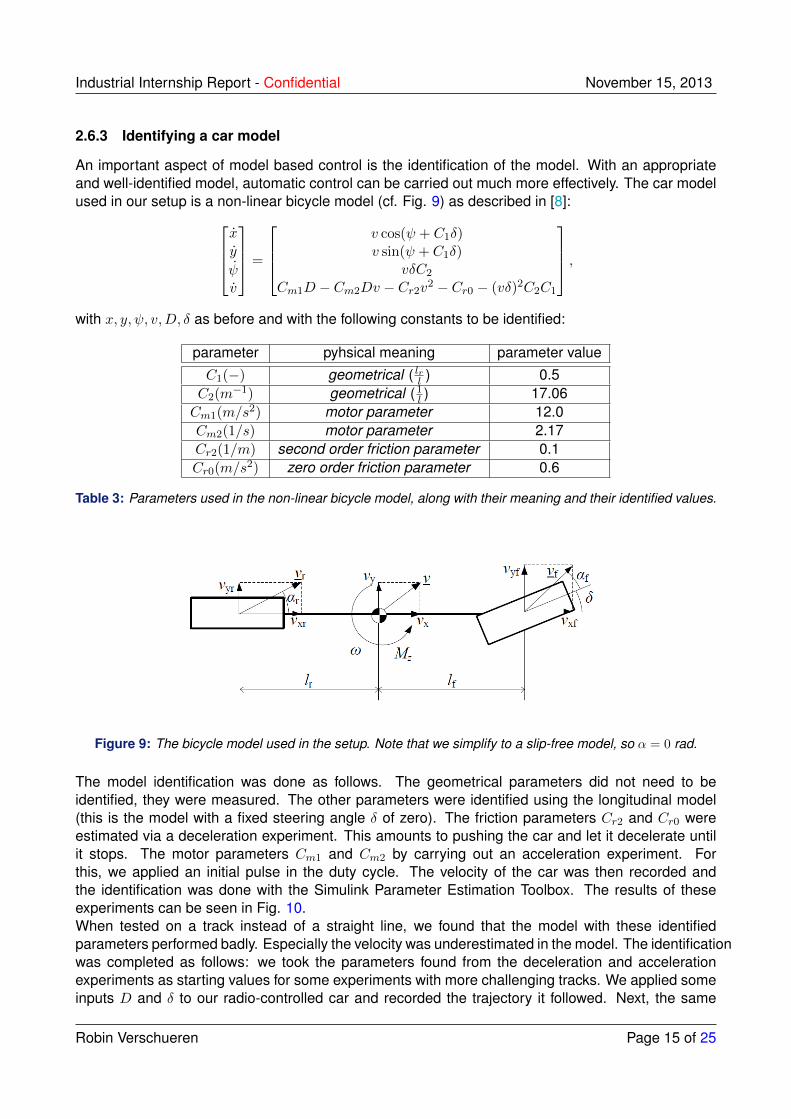
An important aspect of model based control is the identification of the model. With an appropriateand well-identified model, automatic control can be carried out much more effectively. The car modelused in our setup is a non-linear bicycle model (cf. Fig. 9) as described in [8]:

xy

ψv

=

v cos(ψ + C1δ)v sin(ψ + C1δ)

vδC2

Cm1D − Cm2Dv − Cr2v2 − Cr0 − (vδ)2C2C1

,with x, y, ψ, v,D, δ as before and with the following constants to be identified:

parameter pyhsical meaning parameter valueC1(−) geometrical ( lrl ) 0.5C2(m

−1) geometrical (1l ) 17.06Cm1(m/s

2) motor parameter 12.0Cm2(1/s) motor parameter 2.17Cr2(1/m) second order friction parameter 0.1Cr0(m/s

2) zero order friction parameter 0.6

Table 3: Parameters used in the non-linear bicycle model, along with their meaning and their identified values.

Figure 9: The bicycle model used in the setup. Note that we simplify to a slip-free model, so α = 0 rad.

The model identification was done as follows. The geometrical parameters did not need to beidentified, they were measured. The other parameters were identified using the longitudinal model(this is the model with a fixed steering angle δ of zero). The friction parameters Cr2 and Cr0 wereestimated via a deceleration experiment. This amounts to pushing the car and let it decelerate untilit stops. The motor parameters Cm1 and Cm2 by carrying out an acceleration experiment. Forthis, we applied an initial pulse in the duty cycle. The velocity of the car was then recorded andthe identification was done with the Simulink Parameter Estimation Toolbox. The results of theseexperiments can be seen in Fig. 10.When tested on a track instead of a straight line, we found that the model with these identifiedparameters performed badly. Especially the velocity was underestimated in the model. The identificationwas completed as follows: we took the parameters found from the deceleration and accelerationexperiments as starting values for some experiments with more challenging tracks. We applied someinputs D and δ to our radio-controlled car and recorded the trajectory it followed. Next, the same



(a) Deceleration experiment (b) Acceleration experiment

Figure 10: Parameter identification experiments

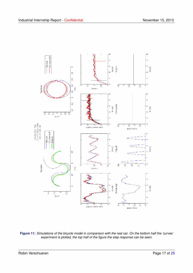
inputs were applied to our model, that was run in MATLAB/Simulink in open loop. This means ourmodel was driving as if it were blind. Lastly, the model parameters were tuned and the model wassimulated iteratively until the model trajectory fitted the real trajectory well enough.The first combination of inputs were obtained by following a curved trajectory, as can be seen in theleftmost half of Fig. 11. Also a step response was tested, as can be seen in the right half of thepicture. As can be seen, this model is adequate enough to be used in an MPC algorithm: the speedis followed closely, as well as the yaw rate ω. The position in the ’curves’ experiment is not thatwell followed by the model, but for rather short prediction horizons (cf. MPC), this will do. Followingthe speed and rotational speed is more important, because the reference trajectory is at a constantspeed. Otherwise, the car will lag more and more behind over time. The final parameter set that waschosen can be found in Table 3.

2.6.4 PID control on the final track

A last accomplishment that was made for Milestone 2 was the testing of the PID controller on the finaltrack. This provoked some minor difficulties, a re-tuning of the proportional gains had to be made forexample. Also a re-calibration was needed. The extrinsic calibration is unavoidable on a new racetrack.The tuning of the three gains (Klateral,Klongitudinal and Korientation) of the proportional controlleris done first in simulation, and then tested on the real setup. A good set of gains seems to beKlateral = 2,Klongitudinal = 4,Korientation = 0.5. This is what could be expected: diminishing thelateral error is the most important, whereas if the car has the right orientation is not crucial for trackingthe centerline; it will correct its orientation by trying to track the centerline automatically.At a speed of 1.1m/s, this gives a quite satisfactory performance for the real car (Fig. 12a). However,if we turn up this reference velocity, the performance deteriorates. For vref = 1.35m/s, this is shownin Fig. 12a. Note the bottom left corner, where the car almost hits the border of the track. Apossible solution to this deviation from the centerline would be to increase the gain on the lateralerror. However, doing this, creates oscillations in the car behavior (Fig. 12b). A last illustration ofthe behavior of the proportional controller is where the gain on the lateral error is too low: this is alsoshown in Fig. 12b. Here, the car drives into the wall after the first corner; the proportional controllerhas no clue that the wall is there.



Figure 11: Simulations of the bicycle model in comparison with the real car. On the bottom half the ’curves’experiment is plotted, the top half of the figure the step response can be seen.



−1 −0.5 0 0.5 1 1.5−1.8

−1.6

−1.4

−1.2

−1

−0.8

−0.6

−0.4

−0.2

0

0.2

x (m)

y (m

)

vref

= 1.1 m/s

vref

= 1.35 m/s

(a) The performance of the car for tracking at twodifferent reference velocities for the proportional

controller.

−1 −0.5 0 0.5 1 1.5−1.8

−1.6

−1.4

−1.2

−1

−0.8

−0.6

−0.4

−0.2

0

0.2

x (m)

y (m

)

Ky = 10

Ky = 1

(b) Car trajectory for different gains for the lateralerror (Klateral = 10,Klateral = 1). Note the

oscillations in the path for the higher gain, whichis unnatural behavior. Setting the gain lower

drives the car to the wall.

Figure 12: The performance of the proportional feedback controller on the final track.


The last two weeks of the internship were used for the design of an MPC controller for trajectorytracking.

2.7.1 Problem formulation

The goal of this part of the project is the tracking of a predefined trajectory. In a first stage, this will bethe tracking of the centerline. Afterwards, tracking of an online computed trajectory will be attempted.The strategy for the design of the MPC tracking is to reformulate the problem as a regulation problem.This means that we will try to drive the error state to zero instead of tracking a time-varying trajectory.A detailed explanation of the reformulation to error states can be found in appendix B. The usedsymbols and their meanings can be found in Table 4.

nx normalized longitudinal errorny normalized lateral errornψ normalized error on the orientationnv normalized error on the speedu1 simplified steering inputu2 simplified duty cycle inputT sampling time

Table 4: Symbols used in the MPC regulation formulation.

Note that we simplify our inputs to the system:

u1 = vδC2 − vnκ (12)

u2 =a− anvn

(13)



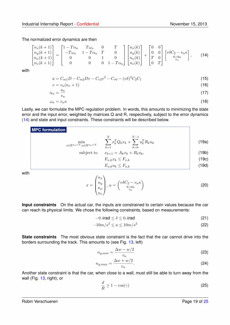
The normalized error dynamics are thennx(k + 1)ny(k + 1)nψ(k + 1)nv(k + 1)

=

1− Tαn Tωn 0 T−Tωn 1− Tαn T 0

0 0 1 00 0 0 1− Tαn

nx(k)ny(k)nψ(k)nv(k)

+

0 00 0T 00 T

[vδC2 − vnκa−anvn

], (14)

with

a = Cm1D − Cm2Dv − Cr2v2 − Cr0 − (vδ)2C2C1 (15)v = vn(nv + 1) (16)

αn =anvn

(17)

ωn = vnκ (18)

Lastly, we can formulate the MPC regulation problem. In words, this amounts to minimizing the stateerror and the input error, weighted by matrices Q and R, respectively, subject to the error dynamics(14) and state and input constraints. These constraints will be described below.

minx∈Rnx×N ,u∈Rnu×N

N∑k=1

xTkQkxk +N−1∑k=0

uTkRkuk

subject to xk+1 = Akxk +Bkuk,

Ex,kxk ≤ Fx,kEu,kuk ≤ Fu,k

MPC formulation

(19a)

(19b)(19c)(19d)

with

x =

nxnynψnv

, u =

(vδC2 − vnκ

a−anvn

)(20)

Input constraints On the actual car, the inputs are constrained to certain values because the carcan reach its physical limits. We chose the following constraints, based on measurements:

−0.4rad ≤ δ ≤ 0.4rad (21)

−10m/s2 ≤ a ≤ 10m/s2 (22)

State constraints The most obvious state constraint is the fact that the car cannot drive into theborders surrounding the track. This amounts to (see Fig. 13, left)

ny,min =∆w − w/2

vn(23)

ny,max =∆w + w/2

vn. (24)

Another state constraint is that the car, when close to a wall, must still be able to turn away from thewall (Fig. 13, right), or

d

R≥ 1− cos(γ) (25)



Figure 13: State constraints on the car needed for the MPC formulation.

2.7.2 Implementation

The presented problem formulation matches that of a linear MPC problem: it contains a quadraticcost function with linear state and input constraints. This problem can be formulated as a genericQP (Quadratic Program). This was done as described in [9]. To solve the resulting QP, we usedthe qpOASES software written by Joachim Ferrea et al. ([10]). This software provides a Simulinkinterface, as well as tailored C++ code, so it fits nicely into our project. The workflow remains thesame: simulate a controller, then export the code and build it on the Debian computer.

2.7.3 Trajectory Tracking: results

The only thing that needs to be done before trying the car on the setup is determining the costmatrices Q and R: with badly chosen weighting matrices, the car will crash into the wall immediatelyor not drive at all. An initial good guess matrices is

Q = diag([1e3, 1e3, 1e− 7, 5]), R = diag([1e− 2, 1e− 2]).

The results of a run with these values can be seen in Fig. 14. In the following experiments, we chosea reference velocity of vref = 1.25m/s.

−1 −0.5 0 0.5 1 1.5−1.8

−1.6

−1.4

−1.2

−1

−0.8

−0.6

−0.4

−0.2

0

0.2

x (m)

y (m

)

(a) Trajectory

0 2 4 6 8 10 120

0.5

1

1.5

2

2.5

time (s)

velo

city

(m

/s)

statesreference

(b) Velocity profile

Figure 14: Experiment with initial values for Q and R.



After some finetuning, we came to the following, better weighting matrices:

Q = diag([1e3, 1.2e3, 1e− 7, 5]), R = diag([2e− 2, 1e− 2]),

with results depicted in Fig. 15. When we compare, we can say that the centerline is followed moreclosely, and also in a smoother way. This follows from the higher weighting on the lateral error (Q2,2)and the higher weighting on the first input. Look for example at the bottom left corner of the trajectory,where the second experiment has a smaller deviation from the centerline. In this way, the car doesnot have to correct afterwards for this deviation. Also the first corner (top right) is taken in a muchbetter way.

−1 −0.5 0 0.5 1 1.5−1.8

−1.6

−1.4

−1.2

−1

−0.8

−0.6

−0.4

−0.2

0

0.2

x (m)

y (m

)

(a) Trajectory

0 2 4 6 8 10 120

0.5

1

1.5

2

2.5

time (s)

velo

city

(m

/s)

statesreference

(b) Velocity profile

Figure 15: Experiment with better values for Q and R.

2.7.4 Trajectory planning

At the end of the internship, a more involved 2-step algorithm was tried out: At the higher level, anonline trajectory optimization is done. At a lower level, this calculated trajectory is tracked using theMPC approach described above. However, this approach caused some problems. The calculationsspawned a lot of NaNs, possibly because of a bug somewhere in the code.

3 Conclusion

As a general conclusion, we might say that the implementation of a practical setup always takesmore time than the understanding and the simulation of theoretical results behind it. However, at theend, seeing a practical result gives a deeper satisfaction than just assessing some simulation results.Also, the goal of the internship is reached: a demonstrator setup was created which was on displayat the European Vehicle Conference of the company. It proved to be a succesful eye-catcher with alot of interested visitors.The more difficult part of the internship, on my behalf, was the integration with Simulink. I wassurprised by how badly the Simulink coder is documented by the vendor. This caused some difficulties,and quite some time spent in debugging.One of the nicest parts of the project was, that in the end, with the trajectory tracking using MPC, youcan really see an impact of certain parameters in the problem. For example, putting a higher penalty



on the y-error (lateral error), you could really see that the car sticked closer to the center. In a PIDcontext, this is generally more difficult.Lastly, the supervision of the internship was very satisfactory. Whenever problems were encountered,or questions came up, help was at hand. Moreover, the working atmosphere turned out to bepleasant.However, the setup can be ameliorated in different ways. First of all, the trajectory planning canbe made to work. Another possibility for a further project is switching from one camera to differentcameras, making it possible to have an arbitrarily large track. Of course, more difficult vehicle modelsand/or switching to non-linear MPC can be investigated also.

4 Link with university programme

For completing the internship, knowledge from following courses (and others) from the mathematicalengineering programme (Master in de Ingenieurswetenschappen: Wiskundige Ingenieurstechnieken)were used:

• Computergestuurde Regeltechniek (H03E8A): The last part of this course deals with linearMPC and the tuning process. Also, experience with Simulink, acquired in this course, came inhandy during the project.

• System Identification and Modeling (H03E1B): Although only linear systems were covered bythis course, it proved to be of great importance in terms of ideas about how to tackle theidentification problem.

• Optimization (H03E3A): Especially the switch from MPC problem formulation to QP problem,and the corresponding terminology, were drawn from this course.

• Technisch-Wetenschappelijke Software (H03F0A): Learning how to compile and link a C++application was crucial for this project, as well as miscellaneous C++ skills and tricks. Also,experience with makefiles proved to be of great convenience.

5 Logbook



Date Activities22/07 introduction with Stijn. Installation of software. Reading ETH thesis

(Rutschmann) and document on Kalman filter23/07 continue reading ETH theses (Keiser). Reading of existing code. Test intrinsic

calibration24/07 measuring intrinsic calibration, problem fixed25/07 looking for blind spots in the vision processing, looking at Kalman filter problem26/07 Kalman filter problem solved, testing of UDP connection29/07 testing of National Instruments Data Acquisition Card30/07 writing of input trackfile parsing. Testing in a straight line31/07 tuning of PID controller. Milestone 1 reached.01/08 Refactoring of the code. Export code to SVN02/08 Looking at delay problem at beginning of car run05/08 Solved delay problem, measuring steering angle06/08 Fitting of steering angle to voltage. Reading about Simulink code generation07/08 Simulink model creation. Simple example of C++ code generation08/08 tuning of Kalman filter. Generation of curves track. SVN troubles09/08 open loop testing of car model on the curves track12/08 oscilloscope measurements for duty cycle13/08 finishing of duty cycle measurements. Start of model identification14/08 model identification: step response. Milestone 2 reached. Building of final track16/08 tested vision processing on final track19/08 fixing of parameters. Reading of ETH thesis (Wunderli)20/08 formulation of MPC problem21/08 tested qpOASES on real time computer22/08 MPC problem implementation23/08 MPC tracking in simulation24/08 MPC tracking succesful, problem was camera connection. Milestone 3 reached.27/08 started MPC planning algorithm28/08 MPC planning works in simulation29/08 MPC planning on track: not satisfactory30/08 there remain problems in the MPC planning. Wrap up



6 Appendix A: Technical details of the setup

Infrared camera: PointGrey Flea 3 Infrared CameraImaging: 1280x1024 at 100 FPSConnection with computer: USB 3.0

Computer: Real-time Debian systemIntel Core i3-3220 @ 3.3 GHzOS: Debian 7.0 ’Wheezy’Kernel: Linux 3.8.13 with Preempt RT Patch

DAQ card: National Instruments PCI-62294 analog outputs, 32 analog inputs, 48 digital I/ODriver software: ni pcimio from Comedi library

Race Car: Kyosho dNaNo FX-101 ASF2.4GHz System

RC-controller: PERFEX KT-18 Transmitter 2.4GHz

7 Appendix B: from states to error states

The non-linear bicycle model is as follows:xy

ψv

=

v cos(ψ + C1δ)v sin(ψ + C1δ)

vδC2

Cm1D − Cm2Dv − Cr2v2 − Cr0 − (vδ)2C2C1

. (26)

We can now switch to error states like this:xeyeψeve

=

cos(ψn) sin(ψn) 0 0− sin(ψn) cos(ψn) 0 0

0 0 1 00 0 0 1

x− xny − ynψ − ψnv − vn

(27)

where [xn, yn, ψn, vn] denotes the nominal trajectory, which is the trajectory that is being tracked, fornow the centerline at a constant speed vn. Next, we would like to determine the error dynamics,which is the result of the combination of the derivative of the error state equation (27) with the vehiclemodel (26):

xeyeψeve

=

v cos(ψe + C1δ)− vn(1− κye)v sin(ψe + C1δ)− vn(κxe)

vδC2 − vnκa− an

(28)

withκ =

ωnvn

(29)



References

[1] Wang and Boyd, Fast Model Predictive Control Using Online Optimization, IEEE Transactionson Control Systems Technology, vol. 18, no. 2, pp. 267–278, Mar. 2010.

[2] LMS Facts and Figures, http://www.lmsintl.com/fact-figures, last accessed August 2nd,2013

[3] Siemens neemt LMS International over, De Tijd, November 8th, 2012,http://www.tijd.be/r/t/1/id/9265205, last accessed August 2nd, 2013

[4] Marc Pollefeys, Visual 3D modeling from Images, University of North Carolina, pp. 21–27, 2001

[5] Camera calibration With OpenCV, http://docs.opencv.org/doc/tutorials/calib3d/camera calibration/camera calibration.html

[6] Hugh Durrant-Whyte, Introduction to Estimation and the Kalman filter, University of Sydney, 2001

[7] Jose Carlos Molina Fraticelli, Simulink Code Generation, april 2012, accessed fromhttp://ntrs.nasa.gov/archive/nasa/casi.ntrs.nasa.gov/20120014980 2012014792.pdf

[8] P. Spengler, C. Gammeter, Modeling of 1:43 scale race cars, ETH Zurich, june 2010

[9] L. Wunderli, MPC Trajectory Tracking, ETH Zurich, april 2011

[10] qpOASES Homepage, http://www.qpOASES.org, 2007-2013


Date post:	25-Feb-2019
Category:	Documents
Upload:	duongnga
View:	236 times
Download:	0 times

Industrial Internship Robin Verschueren - syscop · Industrial Internship Robin Verschueren Authors...

Documents