Inequality and Institutions in 20 th Century America Frank Levy and Peter Temlin 1 MIT-IPC-07-002 Revised June 27, 2007 1 Department of Urban Studies and Planning. MIT, and Department of Economics, MIT. E-Mail: [email protected], [email protected]. We thank Nirupama Rao and Julia Dennett for excellent research assistance and the Russell Sage and Alfred P. Sloan Foundations for financial support. We have benefited from helpful comments from Elizabeth Ananat, David Autor, Jared Bernstein, Margaret Blair, Barry Bosworth, Peter Diamond, John Paul Ferguson, Carola Frydman, Robert Gordon, Harry Katz, Larry Katz, Tom Kochan, David Levy, Richard Murnane, Paul Osterman, Steven Pearlstein, Michael Piore, Dani Rodrik, Emmanuel Saez, Dan Sichel, Jon Skinner, Robert Solow, Katherine Swartz, Ted Truman, Eric Wanner and David Wessel and from seminar participants at NBER, the Sloan School Institute for Work and Employment Research and the New America Foundation.
Transcript
Inequality and Institutions in 20th Century America
Frank Levy and Peter Temlin1
MIT-IPC-07-002
Revised June 27, 2007
1 Department of Urban Studies and Planning. MIT, and Department of Economics, MIT. E-Mail: [email protected], [email protected]. We thank Nirupama Rao and Julia Dennett for excellent research assistance and the Russell Sage and Alfred P. Sloan Foundations for financial support. We have benefited from helpful comments from Elizabeth Ananat, David Autor, Jared Bernstein, Margaret Blair, Barry Bosworth, Peter Diamond, John Paul Ferguson, Carola Frydman, Robert Gordon, Harry Katz, Larry Katz, Tom Kochan, David Levy, Richard Murnane, Paul Osterman, Steven Pearlstein, Michael Piore, Dani Rodrik, Emmanuel Saez, Dan Sichel, Jon Skinner, Robert Solow, Katherine Swartz, Ted Truman, Eric Wanner and David Wessel and from seminar participants at NBER, the Sloan School Institute for Work and Employment Research and the New America Foundation.
The views expressed herein are the authors’ responsibility and do not necessarily reflect
those of the MIT Industrial Performance Center or the Massachusetts Institute of
Technology.
1
Inequality and Institutions in 20th Century America
ABSTRACT
We provide a comprehensive view of widening income inequality in the United States contrasting conditions since 1980 with those in earlier postwar years. We argue that the income distribution in each period was strongly shaped by a set of economic institutions. The early postwar years were dominated by unions, a negotiating framework set in the Treaty of Detroit, progressive taxes, and a high minimum wage – all parts of a general government effort to broadly distribute the gains from growth. More recent years have been characterized by reversals in all these dimensions in an institutional pattern known as the Washington Consensus. Other explanations for income disparities including skill-biased technical change and international trade are seen as factors operating within this broader institutional story. Key words: Income inequality, Institutions, Treaty of Detroit, Washington Consensus JEL Codes: J31, J53, N32
2
Inequality and Institutions in 20th Century America
“A rising tide lifts all the boats”
John F. Kennedy, October 15, 1960
“Simultaneous and identical actions of United States Steel and other leading steel corporations, increasing steel prices by some 6 dollars a ton, constitute a wholly unjustifiable and irresponsible defiance of the public interest.”
John F. Kennedy April 11, 1962 I. Introduction
A central feature of post-World War II America was mass upward mobility: individuals
seeing sharply rising incomes through much of their careers and each generation living better than
the last. The engine of that mobility – John Kennedy’s rising tide – was increased labor
productivity.
It therefore is problematic that recent productivity gains have not significantly raised
incomes for most American workers.2 In the quarter century between 1980 and 2005, business
sector productivity increased by 71 percent. Over the same quarter century, median weekly
earnings of full-time workers rose from $613 to $705, a gain of only 14 percent (figures in 2000
dollars3). Median weekly compensation - earnings plus estimated fringe benefits - rose from $736
to $876, a gain of 19 percent. Detailed analysis of this period shows that college-educated women
are the only large labor force group for whom median compensation grew in line with labor
productivity (Section II).
Since productivity growth expands total income, slow income growth for the average
worker implies faster income growth elsewhere in the distribution. In the U.S. case, growth
2 See for example, Dew-Becker and Gordon (2005), Krugman (2006), Pearlstein ( 2006, a, b), and Tritch (2006), 3 To compare earnings and productivity on a consistent basis, earnings and compensation are adjusted using the GDP deflator.
3
occurred at the very top.4 Thomas Piketty and Emmanuel Saez estimate that the share of gross
personal income claimed by top 1 percent of tax filing units – about 1.4 million returns – rose
from 8.2 percent in 1980 to 17.4 percent in 2005. Among tax returns that report positive wage and
salary income, the share of wages and salaries claimed by top 1 percent rose from 6.4 percent in
1980 to 11.6 percent in 2005.5
To place these developments in historical perspective, we construct the following ratio:
(1) Median Annual Compensation for Full-Time WorkersT Annualized Value of Output per Hour in the Non-Farm Business SectorT
The numerator of (1) is the sum of median annual earnings of full-time workers and the
value of estimated fringe benefits. The denominator of (1) is Non-Farm Business Productivity –
the standard labor productivity measure - expressed as an annual dollar amount.6 We can think of
(1) as a bargaining power index (BPI), the share of total output per worker that the average full-
time worker captures in compensation.
Figure (1) displays this Bargaining Power Index for the last from 1950-2005.7 For
purposes of comparison, Figure (1) also displays the Piketty-Saez estimate of the 99.5th income
percentile on federal tax returns8 – the median income of the top 1 percent of reported incomes –
adjusted for fringe benefits and also normalized by Non-Farm Business Productivity.
4 Slow income growth for the average worker can also mean faster growth of capital income. We return to this point in the Appendix. 5 See Piketty and Saez (2003) and the updating of their figures to 2005 on Emmanuel Saez’ website http://elsa.berkeley.edu/~saez/ (URL). Their calculations are based on pre-tax market income (wages, partnership income, interest, dividends, rents, etc.) excluding transfer payments. A tax filing unit is represents a tax return (which may be single or joint).Piketty and Saez estimate the total number of tax filing units that would occur if all U.S. households filed federal income taxes and figures like the “top 1 percent of tax filing units” refer to the top 1 percent of that estimated number rather than the top 1 percent of those who actually file.. 6 Calculation of this ratio is detailed in the Appendix. 7 Data come from authors ’ tabulations of the 1950 and 1960 Decennial Census and Current Population Survey micro data sets for 1961 and 1963 onward. Data is missing for 1951-59 because Current Population Survey data do not exist in machine readable form for these years and published summaries of the data do not report full time workers separately. 8 This income measure excludes capital gains.
4
Source
Figure 1
Bargaining Power Indices for the Median Full-Time Worker
and for the Piketty-Saez 99.5th Percentile Income (Right Axis)
0.000
0.200
0.400
0.600
0.800
1.000
1.200
1945 1955 1965 1975 1985 1995 2005
0.00
1.00
2.00
3.00
4.00
5.00
6.00
BPI for All FT Workers, ages 21-65
Piketty Saez 95 1/2% income adjusted for
Fringe Benefits and Normalized byProductivity (Right Axis)
Source: See Appendix.
Figure 1 summarizes fifty-five years of economic history. In the “Golden Age” of 1947-
73, labor productivity and median family income each roughly doubled. The Golden Age is
illustrated in Figure 1 by the relatively steady BPI - median compensation of full-time workers
(the numerator) and labor productivity (the denominator) growing at the same rate from 1950 to
the late 1970s. Simultaneously, income equality increased as very high incomes (illustrated by the
99.5th percentile) grew more slowly than labor productivity.
In the 1970s stagflation, median compensation of full-time workers began to lag behind
productivity growth, a trend that accelerated after 1980. In Figure 1, the lag is illustrated by the
BPI declining from .6 in 1980 to .53 in 1990 and to .43 in 2005. This declining bargaining power
5
of the average full-time worker is a useful way to describe why significant productivity growth
since 1980 has translated into weak growth in earnings and compensation.
Very high incomes also lagged productivity growth through the 1970s and early 1980s.
But beginning in 1986, very high incomes began to increase rapidly and have outstripped
productivity growth through the present. In the Piketty-Saez data, the richest 1 percent of tax
filers claimed 80 percent of all income gains reported in federal tax returns between 1980 and
2005.9
Many economists attribute the average worker’s declining bargaining power to skill-
biased technical change: technology, augmented by globalization, which heavily favors better
educated workers. In this explanation, the broad distribution of productivity gains during the
Golden Age is often assumed to be a free market outcome that can be restored by creating a more
educated workforce.
We argue instead that the Golden Age relied on market outcomes strongly moderated by
institutional factors. Following the literature on economic growth that emphasizes the role of
institutions in economic outcomes, we argue that institutions and norms affect the distribution of
economic rewards as well as their aggregate size. Our argument leads to an explanation of
earnings levels and inequality in which skill-biased technical change, globalization and related
factors function within an institutional framework. In our interpretation, the recent impacts of
technology and trade have been amplified by the collapse of the institutions of the post-war years,
a collapse which arose because economic forces led to a shift in the political environment over the
1970s and 1980s. If our interpretation is correct, no rebalancing of the labor force can restore a
more equal distribution of productivity gains without government intervention and changes in
private sector behavior.
9 Details of this calculation are contained in the Appendix.
6
We do not challenge the existence of technology’s and trade’s effects on labor demand
(e.g. Card and DiNardo, 2002). Rather, we argue that technology and trade’s impacts are
embedded in a larger institutional story - a story hinted at by the second John Kennedy quote that
began this paper. Previous writing has examined relationships between inequality and measurable
institutional variables including the rate of unionization, the minimum wage, and tax policy (e.g.
Autor, Katz and Kearny, 2005; Bound and Johnson, 1992; DiNardo, Fortin and Lemieux, 1996;
Feenberg and Poterba, 1993; Gordon and Slemrod 1998; Lee 1999; Reynolds 2006; Saez 2004).
Other authors have focused on historical narrative (e.g. Katz and Lipsky, 1998; Osterman, 1999).
In this paper, we combine data and history in a way that permits telling a more complete story
including the likely origins of institutional shifts. By emphasizing the interplay among
productivity, inequality, and the earnings growth of average workers we are also better able to
describe the impact of current trends on economic life. We call the post-World War II
institutional arrangements the Treaty of Detroit, after the most famous labor–management
agreement of that period. This agreement was replaced in the 1980s and surrounding years by
another set of institutional arrangements we call the Washington Consensus.10 As we will
describe, the decisions to strengthen or to abandon these institutions were made by many people
in complex economic and political settings.
We develop this argument in the sections that follow. Section II describes the evolving
nature of labor demand and presents the data that frame our argument. Section III describes the
institutional arrangements that originated in the Great Depression and helped to distribute
productivity gains broadly from 1947 to 1973. Section IV describes the way in which the post-
1973 productivity slowdown and associated stagflation ultimately led to the arrangements’
10 This term normally is used for LDCs, but the spirit of this concept applies well to the changing institutions within the United States. We use the term here to refer to the microeconomic policies of deregulation and privatization of the consensus, not the macroeconomic policies of fiscal discipline and stable exchange rates. See Willisamson, 1990, pp. 7-24.
7
collapse, to be replaced by institutions that made the labor market particularly vulnerable to
extreme effects of technical change and trade – a vulnerability that is not as evident in most other
industrialized countries. Our description focuses more on the earlier institutions than the later
ones as they are less familiar. Section V concludes by considering the implications of our story
for policy.
II. The Evolving Nature of Labor Demand
For over a decade, the economist’s primary explanation for income inequality has been
skill-biased technical change.11 While the explanation has been refined over time, its core is
unchanged.12 Technology, perhaps augmented by international trade, is shifting demand toward
more skilled workers faster than labor supply can adjust. This explanation of earnings inequality
has resonated strongly with the public as well as government policy. Educational improvement
has been a central policy focus at all levels of government. Equally important, many government
officials describe educational differences as the central driver of inequality, as in the August 1,
2006 remarks of Treasury Secretary Henry M. Paulson:
…. we must also recognize that, as our economy grows, market forces work to provide the greatest rewards to those with the needed skills in the growth areas. This means that those workers with less education and fewer skills will realize fewer rewards and have fewer opportunities to advance. In 2004, workers with a bachelor's degree earned almost $23,000 more per year, on average, than workers with a high school degree only. This gap has grown more than 60 percent since 1975.13
11 See Levy and Murnane (1992) for a history of how earnings inequality became a prominent issue in labor economics. 12 In one refinement, technology is now assumed to substitute for mid-skilled workers rather than the lowest skilled workers (Autor, Levy and Murnane 2003, Autor Katz and Kearny, 2006). In a second refinement, the steady growth of earnings inequality among observationally similar workers in the Current Population Survey was first described as measuring returns to unobserved dimensions of skill (Juhn, Murphy and Pierce, 1993). It is now identified with increasing year-to-year earnings volatility (Gottschalk and Moffitt, 1994) or as an artifact of particular data sets (Lemieux, 2006) 13 http://www.treasury.gov/press/releases/hp41.htm. The remarks were delivered at Columbia University.
8
As in Paulson’s remarks, most discussion of these forces is framed in levels of formal
schooling – e.g. college versus high school. But the theory of skill-related demand applies equally
well to differences among workers with the same quantity of formal schooling.
Figure 2 displays one such difference based on the salaries of new associates in Wall
Street law firms. In standard labor market data, these new lawyers would be classified as men,
ages 25-34, with post-bachelors education (until fairly recently, women female associates were
rare in Wall Street firms). In 1967, a new associate at Cravath, Swain and Moore earned about
$49,500 in 2005 dollars (Galanter and Palay, 1991, p. 24). This salary, which excludes fringe
benefits and bonuses, was 14 percent higher than median earnings of all full-time male workers,
ages 25-34, with post-bachelors education.
Figure 2
Median Earnings of All 25-34 Year old Men with Graduate Education and Starting Associate
Salsries in Wall Street Law Firms, 1967 and 2005 (2005 dollars)
$0
$20,000
$40,000
$60,000
$80,000
$100,000
$120,000
$140,000
1967 2005
Median Earnings of 25-34 Year Old Men withPost BA Education (excludes fringes)
Approximate Starting Salary of New Associatesin Marjor NY Law Firms - e.g.Cravath, Swainand Mooore (excludes bonuses and fringes)
Source: Galanter and Palay, 1991, p. 24; Marin Levy personal communication.
9
In 2005, a starting associate at Cravath earned about $135,000, excluding bonuses and
fringes. The gap between this salary and the median salary of 25-34 year old men with post-
bachelors education had opened from 14 percent to 120 percent. The salaries of Wall Street
lawyers, from associate to partner are often described as winner-take-all salaries - an extreme
form of skill-based inequality and, in fact, Alfred Marshall (1947) used lawyers as an example
when he first described winner-take-all markets in 1890s England.14 The question is why such
salaries were far less common in 1950s and 1960s America.
Consider next workers whose education stopped with a bachelor’s degree – hereafter,
BA’s. The common understanding of skill-biased technical change suggests demand for such
workers should be increasing. But as more people attend college (and more college graduates go
to graduate school), it is plausible that today’s median BA is “less skilled” than the BA of 10 or
20 years ago. Given these opposing forces, it is reasonable to ask whether the compensation of the
“median” BA has kept pace with the growth of labor productivity.
Answering this question requires two refinements. First, even if economy-wide
productivity is constant, an individual’s compensation typically increases with age and
experience, and the age of the “median” BA has increased over time.15 To avoid the spurious
effect of age on compensation, we divide BA’s by age (and, for similar reasons, by gender).
Second, the standard measure of Business Productivity also includes potentially spurious age and
education effects. Since 1950, the labor force has become more educated and experienced and this
changing workforce composition has increased productivity growth above what it otherwise
14 A winner-take-all market is one where the highest ranked participants get rewards far larger than those ranked even slightly lower. Such markets often arise in the provision of a complex high stakes service that must be done right the first time – a legal defense, a delicate surgery, a financial merger – where small differences in skills that cannot be taught can have big consequences. The pay of virtually all partners in Wall Street law firms fall into the top 1 percent of reported incomes on tax returns which began in 2005 at $310,000 (the figure excludes capital gains). 15 In an economy without productivity growth, the typical worker still earns more at age 35 than at age 25 but he earns no more than a 35 year-old worker had earned twenty or thirty years earlier. When a worker benefits from experience premiums and economy-wide productivity growth, individual wage gains are larger and each generation earns more than previous generations. See Frank and Cook (1995) for more discussion.
10
would have been. If “compensation-growing-faster-than-productivity” is to have a consistent
meaning over time, it is necessary to remove labor force composition effects from the annual rate
of productivity growth, a straightforward procedure.16
Figure 3 displays the BPI for six groups of workers: male and female BA’s, ages 25-34,
35-44 and 45-54. In each case, calculations are similar to Equation 1 except that the numerator is
now based on median compensation of a particular group of full-time workers – e.g. 35-44 year-
old female BA’s – and Non-farm Business Productivity in the denominator has been adjusted for
labor force composition effects.17 Figure 4 displays similar information for men and women
whose education stopped at High School.18
16 We thank Larry Katz for this point. Labor composition effects on productivity were taken from "Changes in the Composition of Labor for BLS Multifactor Productivity Measures, 2005” Bureau of Labor Statistics, March 23, 2007 http://www.bls.gov/mfp/mprlabor.pdf, Table 3. We thank Dan Sichel for guidance on using these data. 17 Calculations are detailed in the Appendix 18 CPS data do not allow distinguishing persons with a high school diploma and persons with a General Equivalency Degrees (GED).
11
Figure 3
Bargaining Power Indices for Male and Female BA's,
ages 25-34, 35-44 and 45-54
0.000
0.200
0.400
0.600
0.800
1.000
1.200
1.400
1945 1955 1965 1975 1985 1995 2005
Male 45-54 BA
Male 35-44 BA
Male 25-34 BA
Female 45-54 BA
Female 35-44 BA
Female 25-34 BA
Figure 4
Bargaining Power Indices for Male and Female HS Graduates,
ages 25-34, 35-44 and 45-54
0.000
0.100
0.200
0.300
0.400
0.500
0.600
0.700
0.800
0.900
1.000
1945 1955 1965 1975 1985 1995 2005
Male 45-54 HS
Male 35-44 HS
Male 25-34 HS
Female 45-54 HS
Female 35-44 HS
Female 25-34 HS
12
Source (Tables 3 and 4): See Appendix.
The central feature of Figures 3 and 4 is the difference in men’s and women’s patterns.
For all groups of men – both BA’s and high school graduates - the median worker’s compensation
grows roughly in line with productivity until some date between 1970 and 1980. After that date
(which varies by group) the median worker’s compensation lags increasingly behind productivity
growth.19 For all groups of women, the median worker’s compensation tracks productivity
growth more closely through the entire 55 years. In our terms, the post-1980 partial convergence
of men’s and women’s compensation arose because the average woman’s compensation claimed a
roughly constant share of output per worker while the average man’s compensation claimed a
declining share.20
A closer look at the data for men shows that median compensation begins to lag
productivity first among BA’s and then among high school graduates. Among male BA’s, the first
declines in the BPI appear in early 1970s among 25-34 year olds – the baby-boom cohorts going
to college (Freeman, 1976). In subsequent years, declines appear in older age ranges as the young
cohorts age. By contrast, the compensation of all three age groups of male high school graduates
begins to sharply lag productivity around 1980, suggesting a structural shift, a point to which we
will return.
A closer look at the data for women shows that the BPI’s of women high school graduates
declines steadily, though at a much slower rate than the corresponding BPI’s for men. Female
BA’s are the only group in Figures 3 and 4 whose median compensation consistently grows in
line with economy-wide productivity – i.e. whose bargaining power has not declined.
19 A caveat to this description is the absence of data CPS data on full time workers from 1951-1959. Other data – e.g. the way in which median family income tracked productivity growth over this decade – suggests that individual compensation must have traced productivity growth as well. 20 It is beyond this paper’s scope to examine why women’s compensation tracked productivity better than men’s, but possible factors include women’s increased work experience and the decline in occupational segregation.
13
To put these figures in perspective, consider a standard analysis of earnings inequality that
focuses on the relative earnings of college and high school graduates:
(2) Median Earnings of 35-44 Yr.-Old Male BA’s Median Earnings of 35-44 Yr.-Old Male High School Graduates.
This ratio (2) is exactly equivalent to the ratio of the corresponding BPI’s in Figures 3 and 4: (3) BPI for 35-44 Yr.-Old Male BA’s BPI for 35-44 Yr.-Old Male HS Graduates21
This ratio (3) is separately graphed for men and women in Figure 5 where it tells the familiar
education/earnings inequality story – the ratio of college-to-high school earnings narrows in the
1970s and then increases substantially through the late 1990s before closing slightly in recent
years.
21 The ratios (2) and (3) are equivalent because, as detailed in the Appendix, we construct BPI’s by multiplying both college and high school incomes by the same fringe benefit adjustment and dividing the resulting compensation by the same economy-wide average productivity figure.
14
Figure 5
BA/High School Earnings Premium for 35-44 Year-Old Male and Female Full-Time Workers
0
0.5
1
1.5
2
2.5
1945 1955 1965 1975 1985 1995 2005
35-44 Year Old Men
35-44 Year Old Women
Source: Authors’ Tabulations of Current Population Survey.
When Figures 5 and 3 are taken together they show that the college-high school premium
is only one part of the technology-trade/skill story. The story’s second part asks whether
technology and trade still permit the compensation of the average college graduate to grow in line
with productivity – i.e. is the average bachelor’s degree still sufficient to catch the rising tide? In
the case of men, at least, the answer is no. More generally, something over three-quarters of the
labor force currently face insufficient demand to keep compensation growing in line with
economy-wide productivity.
We argue that while the relatively weak demand for BA’s is fairly recent, it represents an
old phenomenon: the periodic inability of the free market to broadly distribute the gains from
productivity. In particular, the potential for this problem existed in the Golden Age but the
15
problem was largely overcome by economic institutions and norms. The composition of the labor
force was, of course, much different then. In 1940, only five percent of the labor force had a
bachelor’s degree. Unemployment in the Depression had been concentrated among the less
educated and less skilled members of the labor force, and it was largely for these workers that the
New Deal erected a new structure of institutions and norms (US Bureau of the Census, 1975, 380;
Margo, 1991).
This result was a decline in income inequality that was reinforced by the controls of World
War II and produced a broad distribution of productivity gains for at least another quarter
century As Piketty and Saez (2003) write:
The compression of wages during the war can be explained by the wage controls of the war economy, but how can we explain the fact that high wage earners did not recover after the wage controls were removed? This evidence cannot be immediately reconciled with explanations of the reduction of inequality based solely on technical change as in the famous Kuznets process. We think that this pattern or evolution of inequality is additional indirect evidence that nonmarket mechanisms such as labor market institutions and social norms regarding inequality may play a role in setting compensation at the top. (pp. 33-34)
We agree and in the sections that follow, we show how these non-market mechanisms
distributed productivity gains broadly while limiting the extent of very high incomes —at least
until the mechanisms broke down.
III. Norms, Institutions and the Golden Age.
The non-market mechanisms that shaped the postwar Golden Age had roots in the Great
Depression and the New Deal. At first glance, it is surprising that norms and institutions –
microeconomic policies – grew out of a macroeconomic crisis. But macroeconomic policy as we
now understand it did not exist in the Great Depression—Keynes’ General Theory was not
published until 1936.
16
In 1933, Roosevelt’s first year in office, unemployment stood at nearly 25% and
microeconomic policies were apparently the only tools at hand. Lacking a theory of aggregate
demand, Roosevelt’s New Deal policies revolved around something closer to “individual
demand”—a theory that if policy could raise wages and prices to reasonable levels, workers and
producers would earn enough money to stimulate the economy.
This theory was implicit in the first major piece of New Deal legislation, the 1933
National Industrial Recovery Act (NIRA) that gave the government control over employer
contracts, and encouraged labor and industry to negotiate wages, work hours, and other
employment issues (Atleson, 1998). The resulting contracts shortened work hours, increased
wages significantly, and raised prices. With the support of the Roosevelt administration, unions
and collective bargaining began to flourish as employers were hampered in attempts to obstruct
organizational efforts (Temin, 2000). Applying the same logic, NIRA also created the nation’s
first minimum wage set at 25 cents per hour.
The Supreme Court outlawed the NIRA in 1935, citing it as an overreach of federal power
into state interests. Congress responded quickly passing the National Labor Relations Act
(NLRA)—the “Wagner Act”—in the same year, endorsing the rights of labor and limiting the
means employers could use to combat unions, while reestablishing the $.25 minimum wage.
While unions grew dramatically under the NLRA, the post-war system of collective bargaining
may have had its origins more in the unemployment of the Depression than in Roosevelt’s
reaction to that unemployment (Freeman 1998). Economic conditions demanded that something
be done, and unions enjoyed strong public support.22
The NLRA’s minimum wage, like its support of unions and collective bargaining was set
to raise wages significantly. As with our Bargaining Power Index (equation 1) we can put the first
22 In 1936, 76 percent of respondents to a Gallup Poll question said they were in favor of labor unions. Result reported as Roper Center Accession Number 0174236.
17
minimum wage - $.25/hour – in perspective by comparing it to average output per worker in the
economy:
(4) Annual Earnings at the Minimum WageT Annualized Value of Output per Hour in the Non-Farm Business SectorT
In 1938, annual earnings at the first minimum wage represented 27 percent of the economy’s
average output per worker. Between 1947 and 2005, the value of the minimum wage would
exceed that percentage in only four other years (Figure 6) and stands at something less than half
that percentage today.
Source: Minimum Wage data from U.S. Department of Labor:
http://www.dol.gov/esa/minwage/chart.htm.
Figure 6 Ratio of Annual Earnings at the Minimum Wage to
Economy-Wide Labor Productivity
0.00
0.05
0.10
0.15
0.20
0.25
0.30
0.35
1930 1940 1950 1960 1970 1980 1990 2000 2010
18
New Deal policy also raised taxes on very high incomes. On the eve of Roosevelt’s
election, Hoover raised the top bracket rate sharply from 25% to 63% in an effort to reduce the
federal deficit under the impression that the Depression was over. In 1936, after the economy
began to recover more robustly, Roosevelt raised the top bracket rate further to 79% (Figure 7).
This additional increment was part of a general tax rise that included a tax on undistributed
profits, based on the presumption that the economy had progressed into a normal recovery—a
presumption speedily abandoned in the recession that followed hard on the heels of the higher
taxes (Rosen, 2005). Nonetheless, Roosevelt’s clear goal was to compress the income distribution
using unions and the minimum wage to raise low incomes while using tax rates and moral suasion
to hold down incomes at the top.
Source: Frydman and Saks, 2005.
Figure 7 Top Federal Tax Rate on Labor income
0
0.1
0.2
0.3
0.4
0.5
0.6
0.7
0.8
0.9
1
1930 1940 1950 1960 1970 1980 1990 2000
19
While New Deal policies were strongly pro-organized labor, the policies could not provide
the outcome labor wanted most – an economy growing rapidly enough to bring back full
employment. In 1937, five years into the New Deal, the unemployment rate had fallen only to
14.3 percent. Labor-business relations remained contentious and were marked by continued
frequent strikes. When the economy reentered recession in 1938, part of the public blamed
unions, and public support for unions weakened moderately.23
When the United States entered World War II, mobilization and production became the
focus of the economy. The war induced a labor shortage, ending Great-Depression
unemployment, and the principles of efficient manufacturing became ingrained into America’s
economic philosophy. Stability became the government’s goal, and bargaining solidity was
critical to achieving uninterrupted production.
Although policies of arbitration and dispute resolution through administrative means
demonstrated the principles of uninterrupted production, workers feared being left out of wartime
prosperity, and threats of labor action remained high. AFL-CIO action from 1939 to 1941 and
wildcat strikes during 1943 and 1944 interrupted wartime production and impacted munitions
production. Actual wartime strikes were brief and uncommon, but they damaged the public
perception of unions.24 The military saw unions as detrimental to the war effort, and they took
several initiatives to undercut union power (Koistinen, 2004).
The government created the National Defense Mediation Board in 1941 to settle labor
disputes and replaced it a year later with the National War Labor Board (NWLB). These
23 In 1938, 58 percent of respondents to a Gallup Poll question said they were in favor of labor unions, down from 76 percent in 1936 and 1937. Result reported as Roper Center Accession Number 0274556. The 1938 result is not strictly comparable to earlier years because the 1938 question permitted a response of No Opinion (14 percent) while earlier years did not. 24 In 1942, the National Opinion Research Center asked: “After the war, do you think the Federal government should regulate...labor unions more or less than it did before the war started (say 1938)?” More = 60 percent, Same = 13 percent, Less = 6 percent, Depends or Don’t Know = 15 percent. Roper Center Accession Number 0362578.
20
initiatives achieved no-strike and no-lockout pledges from unions and companies and effectively
froze wages for the duration of the war. The agreement created an uneasy peace, but it was a
source of tension between unions, the government, and industry throughout the war.
The Revenue Act of 1942 taxed significant wartime earnings, but the government did not
include workers’ pensions and health insurance as profits, providing employers with an incentive
to avoid the tax by supplementing labor benefits. The NWLB also decided that employer
contributions to benefit plans should not be included as wages, further assisting labor. Industry
reluctantly supported these benefits, mostly as an attempt to discourage union membership, and
the wartime institutions produced a dramatic fall in the wage dispersion from 1940 to 1950 as the
NWLB and other institutions homogenized wages (Goldin and Margo, 1992). The legacies of the
NWLB included both the procedures forced on businesses to promote unions, including checking
off union dues, and the formative experience of many people involved with the NWLB who went
on to become labor-relations experts after the war (Harris, 1982, Chap. 2; Edelstein, 2000).
As the war drew to a close, many feared that the end of wartime strike controls would
bring labor market disruption and the potential for a second Great Depression. Hoping to avoid
this outcome, President Truman convened a three-week National Labor-Management Conference
in November 1945 to discuss post-war labor relations (Harris, 1982, Chap. 4). From today’s
perspective, two features of the conference stand out. The first was the small guest list – 36
business, labor and public officials. The short list was commentary on both the oligopolistic,
regulated structure of industry and the concentration of union power. As Katz and Lipsky (1998,
p. 147) write:
Truman’s notion that an elite tri-partite group could ‘furnish a broad and permanent foundation for industrial peace and progress’ apparently was widely shared by the press and general public.
21
The meeting’s second important feature was the implication that even in peacetime,
business-labor relations would remain a tri-partite process with government actively involved
with government as the third man in the ring.25 Truman did not expect business-labor
tranquility—strikes were the reaffirmation of unions’ power. But Truman believed the
government had to keep business-labor conflict within bounds for the economy to prosper. His
authority on this matter was enhanced by the heavy regulation of interstate transportation,
telecommunication and other industries. While the conference did not reach agreement on many
specific proposals, Truman’s position received board support. An example is a statement made by
Eric Johnston, president of the U.S. Chamber of Commerce:
Labor unions are woven into our economic pattern of American life, and collective bargaining is a part of the democratic process. I say recognize this fact not only with our lips but with our hearts.26 These two characteristics would be codified in the Treaty of Detroit, a private treaty that
codified and extended institutions for labor relations that had begun in the Depression and been
enlarged in the very different environment of the war. The continuity of these institutions
suggests strongly that they were not the result of individual historical accidents, but rather the
outcome of complex negotiations and bargaining between the government, big business, and
unions.
For example, Truman retained a high top bracket income tax rate on labor income in
another extension of Depression-era policy. As Frydman and Saks (2005) and others have noted,
tax rates are endogenous, reflecting in part the social norms of the time. The high top-bracket rate
on labor income and an active government presence in the economy were clear signals to limit
high salaries. In their historical study of executive compensation (including the value of options)
Frydman and Saks (2005) write: 25 The phase refers to the referee in a boxing match. See, for example, Goldstein 1959. 26 Erik Johnston, President’s National Labor-Management Conference, 1946, General Committee, 52. quoted in Katz and Lipsky (1988) See also, Harris (1982)..
22
[Our econometric ] results suggest that, had tax rates been at their year 2000 level for the entire sample period, the level of executive compensation would have been 35 percent higher in the 1950s and 1960s. (p. 31, brackets added)
We return shortly to the interaction of tax rates and norms.
Despite Truman’s best efforts, the postwar transition was difficult. At the war’s end,
organized labor erupted with an average 3.1% of the workforce involved each year in work
stoppages between 1947 and 1949 (Figure 8). The conflict, however, only modestly diluted public
support for unions.27 Business, for its part, supported the Taft-Hartley Act of 1947 which defined
restrictive administrative policies to constrain unions. Although the Taft-Hartley Act clearly
rolled back some union gains from the Depression and war, it fell far short of dismantling them
entirely.
Figure 8
Persons Engaged in Work Stopages as Proportion of All Workers
0.000
0.005
0.010
0.015
0.020
0.025
0.030
0.035
0.040
0.045
0.050
1947
1950
1953
1956
1959
1962
1965
1968
1971
1974
1977
1980
1983
1986
1989
1992
1995
1998
2001
2004
Persons in Work Stopages as Percent of AllWorkers
Source: Data on work stoppages from U.S. Bureau of Labor Statistics: http://stats.bls.gov/news.release/wkstp.t01.htm
27 People remained strongly supportive unions per se but a significant proportion favored restraining their power. In 1949, the Gallup Poll asked: “As things stand today, do you think the laws governing labor unions are too strict or not strict enough?” Too Strict- 17%; About Right- 24%, Not Strict Enough 46%, No Opinion – 13%. Roper Accession Number 0170069
23
It was in this context, in late 1948, that Walter Reuther and his advocates assumed control
over the United Auto Workers (UAW). The relationship between the UAW and the “Big Three”
automakers (Ford, GM, and Chrysler), previously plagued by turmoil, entered a new phase of
negotiation. Reuther, an experienced labor leader, hoped to overhaul industrial relations in favor
of labor interests, but the postwar setting created significant obstacles for his social vision.
Workers faced dramatic inflation, wages remained inert, and the government’s cold-war spending
policy indicated the situation would not improve.
Charles Wilson, the CEO of GM, was aware that inflationary pressures generated by cold-
war military spending promised to be a permanent feature of the economic scene. GM had
recently begun a $3.5 billion expansion program that depended on production stability, and stress
created by inflation could instigate the unions to interrupt production with a devastating strike.
Reuther also had recently survived an assassination attempt, indicating to GM the UAW’s internal
fissures. For Wilson, a long-term wage concession would be a profitable exchange for guaranteed
production stability (Lichtenstein, 1995).
GM’s two-year proposal to the UAW included an increase in wages and two concepts
intended to keep wages up over time. The first, a cost-of-living adjustment (COLA), would allow
wages to be influenced by changes in the Consumer Price Index, adjusting for rising inflation.
Second, a two-percent annual improvement factor (AIF) was introduced, which would increase
wages every year in an attempt to allow workers to benefit from productivity gains. The UAW, in
exchange, would allow management control over production and investment decisions,
surrendering job assignment seniority and the right to protest reassignments. Reuther and his
advisors initially opposed the plan, believing the AIF formula to be too low and the deal to be a
profiteer’s bribe signaling the end of overall reform. Workers needed assistance, however, and
Reuther agreed to the plan and wage formulas, but “only because most of those in control of
24
government and industry show no signs of acting in the public interest. They are enforcing a
system of private planning for private profit at public expense” (Lichtenstein, 1995). The contract
was signed in May, 1948.
For the next two years, labor saw wage increases and gains from productivity. GM
enjoyed smooth, increasing production, and established a net income record for a US corporation
in 1949 (Amberg, 1994). When the time period for the contract ended, the UAW and GM readily
agreed to a similar plan that included several changes. A pension plan was initiated, initially
through Ford in 1949, which had an older workforce and progressive managers (Lichtenstein,
1987). The resulting plan was presented to GM as a precedent to create industrial conformity in a
process known as pattern bargaining. GM agreed readily, and the last of the “Big Three,”
Chrysler, agreed after an expensive strike. Agreements to the pension plan ultimately spread to
other industries, including rubber, Bethlehem Steel, and then U.S. Steel (Amberg, 1994). In
addition to the pension plan, GM increased the COLA/AIF formulas and paid for half of a new
health insurance program. The final, five-year UAW-GM agreement was named the “Treaty of
Detroit” by Fortune magazine: “GM may have paid a billion for peace but it got a bargain.
General Motors has regained control over one of the crucial management functions… long range
scheduling of production, model changes, and tool and plant investment.” Wage adjustments and
productivity gains became recognized as necessary and just, union membership increased, and
industry reaped the profits from the Treaty of Detroit’s stability (Lichtenstein, 1995).
The Korean War’s outbreak in 1950 immediately threatened the agreement as the UAW
and GM had to intervene to prevent the government from freezing wages. Inflationary
adjustments during Korea were not fully reflected by the COLA formula, causing disappointment
in the UAW. Other issues created by the Treaty of Detroit also caused friction, specifically the
emphasis on debating national policy over local factory floor issues. The UAW shifted its focus,
25
fighting for standardized monetary and fringe benefits while workers became frustrated over shop
terms and job assignments. The problem was exacerbated by the bureaucratization of grievance
disputes, which created a backlog of complaints about daily working conditions.
Despite these problems, the Treaty of Detroit initiated a stable period of industrial
relations. The use of collective bargaining spread throughout industry, and even non-union firms
approximated the conditions achieved by unions in an extension of pattern bargaining. Although
the strict application of this term refers to the dynamics of union negotiations in large firms, a
looser version was pervasive (Chamberlain and Kuhn, 1986). The NLRA provided a regulatory
framework for labor to organize a significant part of the industrial labor force.
This framework was administered by the National Labor Relations Board (NLRB), set up
in 1935 under the NLRA. Congress explicitly rejected a partisan board composed of labor and
management representatives and opted instead for “impartial government members.” This
concept lasted only two decades, however, and President Eisenhower, the first Republican
president after Roosevelt, appointed management people to the NLRB. This violation of the
original intent of the board was controversial, and the seeds of future controversy were planted,
but the neutrality of the board was more or less preserved (Flynn, 2000).
Unions acknowledged the exclusive right of management to determine the direction of
production in return for the right to negotiate the impact of managerial decisions. Unions were
able to craft an elaborate set of local rules that constrained management in its allocation of jobs
and bolstered the power of unions over jobs (Kochan, 1980; Weinstein and Kochan, 1995).
Simultaneously, managers used the framework of the Treaty of Detroit to tighten their grasp on
production decisions. The inclusion of supplementary unemployment benefits in production
decisions in 1955 gave managers even more control over job descriptions and workplace
decisions, as unions conceded these rights in exchange for direct welfare. Labor complaints had
26
to go through paperwork, and the burden to oppose or modify change was placed on the workers
(Brody, 1980).
The impact of this framework is clear in the pattern of relative wages. Eckstein and
Wilson found in a study of nominal wages in the 1950s that,
Wages in a group of heavy industries, which we call the key group, move virtually identically because of the economic, political and institutional interdependence among the companies and the unions in these industries…. Wages in some other industries outside this group are largely determined by spillover effects of the key group wages and economic variables applicable to the industry (Eckstein and Wilson, 1962).
Changes in these pattern wages were determined by economic variables, according to
Eckstein and Wilson, but the same forces that kept industrial wages in a stable pattern likely
affected the extent of overall wage changes as well. Erickson (1996) extended the concept of
pattern bargaining to include specific contract provisions. He found that they also were
remarkably similar at both inter- and intra-industry levels in the 1970s, although not in the 1980s
as we will see. Katznelson (2005) however reminds us that this pattern of stable conditions and
wages did not extend to all corners of the economy. Black workers and other minority groups
were largely ignored in these negotiations.
Steadily rising wages did not eliminate labor-management conflict (Figure 8). As we have
suggested, the causality ran in the opposite direction with the threat of strike activity motivating
wage growth. By the late 1950s, American business was facing increased global competition and
pressure to minimize labor costs, particularly as the economy was entering recession. Business
also sensed that union momentum might be weakening.28 In response to these circumstances,
business increased their demands and rigidity to create “the Hard Line” in 1958, sparking a series
of strikes (Jacoby, 1997).
28 Though the public, on balance was still supportive. In 1958, 64 percent of respondents to a Gallup Poll question said they were in favor of labor unions, 21 percent disapproved, 13 percent had no opinion 1 percent gave no answer. Result reported as Roper Center Accession Number 0036121
27
Work stoppages eased modestly in the early 1960s as the Kennedy/Johnson administration
stimulated the economy through a pair of tax cuts on investment and incomes respectively.
Because the tax cuts were a first application of Keynesian policy, government economists were
particularly concerned about the potential for inflation. To address this possibility, the Kennedy
Council of Economic Advisors announced a set of wage-price guideposts explicitly suggesting
how productivity gains should translate into wage and price decisions. Walter Heller, the first
chairman of Kennedy’s Council of Economic Advisors, wrote about the policy in 1966:
One cannot say exactly how much of the moderation in wages and prices in 1961-65 should be attributed to the guideposts. But one can say that their educational impact has been impressive. They have significantly advanced the rationality of the wage-price dialogue.
In business, the guideposts have contributed, first, to a growing recognition that rising wages are not synonymous with rising costs per unit of output. As long as the pay for an hour’s work does not rise faster than the product of an hour’s work, rising wages are consistent with stable or falling unit-labor costs. Second, they are helping lay to rest the old fallacy that “if productivity rises 3 percent and wages rise 3 percent, labor is harvesting all the fruits of productivity” Guideposts thinking makes it clear that a 3-percent rise in labor’s total compensation, which is about three fifths of private GNP, still leaves a 3-percent gain on the remaining two fifths – enough to provide ample rewards to capital, as is vividly demonstrated by the double of corporate profits after taxes in the five years between the first quarters of 1961 and 1966. (Heller, 1967, p. 44, italics in the original).
The wage-price guideposts were one of a number of the government’s continued interest
in promoting economic norms. Another was Kennedy’s 1962 public confrontation with U.S. Steel
over steel price increases. The price increase came shortly after Kennedy had persuaded the
United Steel Workers to accept a moderate wage settlement. Kennedy responded to the perceived
betrayal with a blistering press conference – including the second quote that opened this paper –
and the threat of sanctions using government procurement policy.29 Ultimately, the price increases
were rescinded.
29 See the transcript of Kennedy’s press conference on April 11, 1962: http://www.jfklibrary.org/Historical+Resources/Archives/Reference+Desk/Press+Conferences/003POF05Pressconference30_04111962.htm
28
This history is relevant to current debates over the interpretation of growing income share
claimed by the top 1 percent of taxpayers. Feenberg and Poterba (1993) and Gordon and Slemrod
(1998) have argued that this income concentration is to some extent, an artifact of tax law
changes. Reynolds (2006) recently argued that all of the recent growth in high-end inequality is a
tax law artifact.30 Since changes in tax laws frequently reflect changes in societal norms, a focus
on tax laws alone potentially misses important parts of the story.
In this connection, the 1964 tax cut (ultimately passed under Lyndon Johnson) represents
a natural experiment. The legislation included a sharp reduction on the top rate for labor income
(Figure 7) at a time when a CEO receiving a radically increased paycheck risked White House
criticism. That risk helps to explain why the reduced top tax rate produced no surge in either
executive compensation or high incomes per se (Frydman and Saks, 2005; Saez 2005). A related
experiment occurred in 1992 when the Clinton administration’s tax legislation significantly
increased the top marginal rate at a time when the White House showed no inclination to criticize
high incomes. Despite the increased top bracket rate, the share of income claimed by the top 1
percent of tax returns continued to rise rapidly.
While initially successful, the Kennedy-Johnson macroeconomic policies were soon
overwhelmed by events. In 1965, the government began deficit-financing the Vietnam War in an
economy that was already near full employment. By 1969, unemployment had fallen to 3.5
percent and consumer prices were rising at a then high 5.4 percent. In a tight labor market,
debates over automation became increasingly common, as new technology fueled the power
struggle between unions and management for control of decision making and the right to adapt to
P+S Top 99.5 Percentile Income + Fringes(Right Axis)
Productivity Slowdown Begins
Source: See Appendix.
This broad-based income growth benefited daily economic life in three main dimensions:
- An Expanding the Middle Class. By 1964, 44 percent of the population reported itself as middle class, up from 37 percent in 1952. The expanding middle class did not reflect significantly more equal incomes,31 but rather rapid income growth in which more families could afford a single family home, one or more cars, and the other elements of a middle class lifestyle.
- Mass Upward Mobility. A number of studies have shown that intergenerational mobility
within the U.S. income distribution is relatively limited (e.g. Solon 2002). But rapidly rising incomes created a mass upward mobility such that a blue collar machine operator in the early 1970s earned more in real terms than most managers had earned in 1950. Much of a generation could live better than its parents had lived even though their relative positions in the income distribution were similar. 32
- A Safety Net for Industrial Change. In any period, losing a job and finding another can
result in an immediate pay cut reflecting the lost value of firm-specific human capital.
31 While the 99 ½th percentile income had grown slowly, the 95’th and 90’th percentile incomes grew in line with incomes of the middle of the distribution. See Piketty and Saez, op. cit. 32 In the golden age, perceptions of upward mobility were enhanced because the expectations of many people had been formed in the Great Depression. See Levy (1998) for more details.
31
When wages were rising rapidly, a person could take a pay cut and “grow back” into their old pay level in a reasonably short time. When wages are “stagnant” recovery can take much longer strengthening perceptions of a lack of good jobs, (Uchitelle, 2006).
In periods of stagnant wages, these virtues are much harder to come by.33 And by 1970-
71, the economy’s declining ability to produce such benefits was becoming clear. The excessive
stimulation of late 1960s – the Vietnam War deficits – led to inflationary expectations that were
impervious to normal recessions and would become known as stagflation. Additional problems
followed in quick succession: an inflationary supply shock in food (1972-3), another supply shock
in oil (1973-4) and, most important, the collapse of productivity growth after 1973. By 1975, the
unemployment rate had reached 8.5 percent, and inflation was increasing at 8.2 percent. Most real
incomes had stopped rising (Figure 9). Economic problems topped the Gallup Poll’s list of the
nation’s biggest problem for the first time since 1946.34
As with the Great Depression, policy makers faced stagflation with little relevant history
to serve as a guide. Economic theory had followed Keynes in focusing on demand shifts, and
there was no theory of the supply side that related to economic policy. Only in the mid-1970s
was the concept of aggregate supply developed to extend the standard IS-LM model. And as with
the Great Depression, the resulting policy agenda was heavily microeconomic. To combat slow
productivity growth, some economists began to argue for economic restructuring including
removing what they saw as the rigidities of New Deal institutions: unions imposing work rules; a
regulatory regime covering most of the nation’s utilities, telecommunications and interstate
transportation; and high marginal tax rates that they assumed reduced work effort.
Jimmy Carter argued in 1978 that, “The two most important measures the Congress can
pass to prevent inflation … (are) the airline deregulation bill … (and) hospital cost containment
legislation.” He appointed Alfred E. Kahn, chairman of the Civil Aeronautics Board, to head the 33 Immigrants clearly find their jobs improved in these ways by entering the U.S. labor force. But this is an example of cross-section variation of wages and working conditions, while this paper is about time-series variation. 34 See, for example, Roper Center Accession Number 0026306, May 16, 1976.
32
administration’s anti-inflation program. Kahn’s field was government regulation, and his plans
were to reduce regulations that supported monopoly pricing (Carter, 1978; Cowan, 1978). We do
not want to equate Carter and Roosevelt or even economic theory in the 1970s and 1930s.
Instead, we note that unusual macroeconomic events sometimes transcend existing
macroeconomic theory. Before macroeconomics could be expanded to include the aggregate
supply curve in the 1970s, public policy appears to have focused on perceived microeconomic
problems.
In what is now known as the Washington Consensus on economic policy, deregulation
plays a prominent role. The impact of deregulation on wages was not much discussed in the
1970s because blue collar wages, in particular, continued to do fairly well. On the labor market’s
supply side, male high school graduates remained heavily unionized (42 percent – authors’
tabulations) with unionization among female high school graduates at 17 percent. On the labor
market’s demand side, the food and oil supply shocks had stimulated the energy and agricultural
industries while a declining international value of the dollar was expanding global demand for
U.S. manufacturing goods.35 Strong manufacturing, energy and agricultural sectors created what
economic geographers were calling a “Rural Renaissance” (Long and DeAre, 1988) in which the
nation’s heartland was doing well, with resulting demand for blue collar workers, while the east
and west coasts were stagnant.36
In reality the Rural Renaissance was a blue-collar bubble. High demands for agriculture
and domestic energy were temporary while the falling dollar was masking manufacturing’s
35 In 1971, Richard Nixon had abandoned fixed exchange rates as part of his program to deal with inflation, a recognition of the fact that continuing trade deficits were diminishing the country’s exchange reserves. 36 Even at the time it was clear that some of this success was unsustainable. In the early 1970s’ both the auto workers and steel workers unions had signed new contracts in which full cost-of-living adjustments were exchanged for promises of labor peace. At that time, no one anticipated consumer prices doubling over the next ten years. As a result, auto makers and big steel firms became an island in the economy with real wages far higher than even most other unionized occupations. Had exchange rates fallen far enough to bring overall trade flows into balance, auto and big steel would still have been overpriced on world markets.
33
competitive weakness. Unions, perhaps lulled by this temporary prosperity, largely ignored the
need to organize a changing labor market. As labor force composition shifted toward women and
college graduates, many in the service sector, union membership fell to about 27 percent of all
wage and salary workers (private and public), down from 35 percent at the peak of their post-war
strength (Osterman, 1999; Hirsch and Macpherson, 2004).
While the bubble existed, however, wage setting norms interacted with inflation to
markedly increase labor’s share of national income. The ideas embodied in the Treaty of Detroit
were developed in the time of low inflation and high productivity that followed World War II.
From the end of the war through the mid-1960s, real wages rose dramatically but labor’s share of
national income cycled narrowly around 67 percent.37 In subsequent years, inflation accelerated,
productivity growth declined, and wage setting norms – for example, money wages rising roughly
in line with the Consumer Price Index – helped labor’s share to rise to .74 in 1973 and .76 in
1980. Capital’s weak prospects were summarized in the performance of the Dow-Jones Industrial
Average: 903 in January 1965 falling to 876 in January 1980 while the general price level had
more than doubled. The effectiveness of COLA contracts in this inflationary environment put
pressure on the Treaty of Detroit system.
While Carter advanced deregulation and increased competition as solutions to the stagnant
economy, others attacked unions directly. An example was the 1978 failure of a bill reforming
labor law. The bill proposed a set of small, technical changes in labor law that would have
preserved the legal framework in which the Treaty of Detroit labor system had operated. Despite
the small scale of the bill, business mounted a large, inflammatory public campaign against it.
The bill passed the House by a vote of 257 to 163, and it would have passed the Senate as well.
37 We thank Robert Gordon for these estimates of labor’s share that also appear in Dew-Becker and Gordon (2005). The estimates reported here based on compensation only. Gordon and Dew-Becker present a second estimate that adds the labor component of proprietor’s income which raises the level of labor’s share but demonstrates the same variation over time.
34
But employers took a hard line against the bill and arranged to have it stopped by a filibuster.
After a 19-day filibuster, the bill’s supporters failed in their sixth try to muster 60 votes to stop it
and sent the bill back to committee to die (Mills, 1979). The AFL-CIO’s failure to pass this bill
demonstrates that while labor still had the support of most political representatives, it no longer
had enough support to offset the blocking actions in the federal government. In particular,
employers no longer felt the need to share the accommodating views expressed by the president
of the US Chamber of Commerce during Truman’s 1945 conference.
For the remainder of the 1970s, the economy continued to limp along. Unemployment fell
slowly, and weak productivity growth translated economic expansion into additional inflation. By
1979, consumer prices were increasing at 12 percent annually. Shaken financial markets forced
Carter to appoint Paul Volcker, an inflation hawk, as Chairman of the Federal Reserve. Volcker
quickly instituted a strong tight money policy to break inflation quickly. When, in 1980, Carter
was defeated by Ronald Reagan, Volcker’s and Reagan’s policies combined to help dismantle
much of what remained of New Deal institutions and norms.
In Reagan’s first year in office, he made three decisions that proved central to the wage
setting process. He gave Volcker’s tight-money anti-inflation policy his full backing. He
introduced a set of supply-side tax cuts including lowering the top income tax on non-labor
income from 70 to 50 percent to align it with the top rate on labor income. And when the air
traffic controllers union, one of the few unions to support Reagan, went out on strike, he gave
them 48 hours to return to work or be fired. His stance ultimately led to the union’s
decertification.
The firing of the air traffic controllers, the 1978 defeat of labor law reform and the
lowering of tax rates were signals that the third man–government–was leaving the ring. From that
point on, business and labor would fight over rewards in less regulated markets with many
35
workers in an increasingly weak position. Then, in an unanticipated development, Volcker’s tight
money policy further weakened the position of blue collar workers.
With Reagan’s strong backing, Volcker’s policy reduced inflation far more rapidly than
most economists had predicted–from 12.5 percent in 1980 to 3.8 percent in 1982. But by 1982,
Reagan’s tax cuts, combined with little expenditure reduction, had led to projections of large
future deficits. Financial markets, fearing the deficits would be monetized, kept interest rates high
even as inflation fell.38 High real interest rates increased global demand for U.S. securities and
the dollars required to buy them. Between 1979 and 1984, the trade-weighted value of the dollar
rose by 55 percent.
The result was perhaps fifteen years of normal change compressed into five years. U.S.
durable manufacturing firms – a pillar of private sector unionization – were hit first by the deep
recession and then by the high dollar that crippled export sales. More generally, high real interest
rates restricted profitable investment opportunities for mature firms in all industries, making them
targets for takeover activity39. The loss of old line manufacturing jobs together with new
employer boldness put unions under siege. The fraction of all private sector wage and salary
workers in unions fell from 23 percent in 1979 to 16 percent in 1985 (Hirsch and Macpherson,
2004). The unionization rate among male high school graduates fell from 44 to 32 percent
(authors’ tabulations). The Rural Renaissance of the 1970s became the Rust Belt of the 1980s
These changes in the real economy were enabled in part by financial innovations designed
to increase the role of market forces in allocation of capital. An early example was the late 1970s
securitization of mortgages as mortgage-backed bonds. As interest rates rose during the 1970s and
early 1980s, savings and loan institutions were under pressure to sell low-interest mortgages in 38 By 1982, the real interest on three year government securities exceeded 6 percent – three times its normal postwar value. 39 This argument has been developed most fully by Margaret Blair. Blair argues that the lack of investment opportunities helps to explain the growth of “free cash flow” that lies at the center of Michael Jensen’s arguments in favor of corporate takeovers. See Blair and Schary (1993) and Jensen (1997).
36
the hope of reinvesting the proceeds at higher returns. There was little investor interest in buying
individual mortgages but mortgage-backed bonds created a market in which these mortgages
could be sold. The market grew rapidly and, as a byproduct, helped to redefine income norms.
Lewis (1989, p.126) tells the story of Howie Rubin, a late 20’s graduate of Salomon Brothers’
training program who was assigned to trade mortgage-backed bonds. In 1983, Rubin’s first year,
he had generated $25 million of revenue:
…Rubin, like all trainees, was placed in a compensation bracket. In his first year, he was paid $90,000, the most permitted a first-year trader. In 1984, his second year, Rubin made $30 million trading. He was then paid $175,000. He recalls, “The rule of thumb at Harvard [Business School] had been that if you are really good, you’ll make a hundred thousand dollars three years out.” The rule of thumb no longer mattered. In the beginning of 1985 he quit Salomon Brothers and moved to Merrill Lynch for a three year guarantee: a minimum of $1 million a year plus a percentage of his trading profits.
Many of Salomon’s other successful mortgage bond traders soon left the firm for similar offers.
Similarly, junk bonds were developed in part to finance corporate takeovers, shifting
control of the corporation’s assets from the current mangers to shareholders (Jensen, 1997). Here,
too, a byproduct was very high salaries for both the junk bond salesmen and the investment
bankers and lawyers who advised in the transactions. The rapidly growing U.S. Treasuries
market, a result of the Reagan budget deficits, provided additional bond trading opportunities.
Between 1975 and 1984, total credit market debt grew from $2.5 trillion to $7.2 trillion dollars
(nominal dollars). 40
This history is summarized in Figure 10 which shows for selected industries the sum of
compensation and corporate profits - a surrogate for economic rents – per full-time equivalent
employee (FTE). From 1950 through the end of the 1970s, economic rent per FTE in the Finance,
40 Board of Governors of the Federal Reserve System, Flow of Funds Accounts of the United States, various issues.
37
Insurance and Real Estate Industry (FIRE) grew at a rate similar to rates in other industries.
Beginning in the mid-1980s, economic rent per FTE in FIRE grew at an accelerating pace in line
with the expanding bond market and a revived stock market.41
Figure 10
(Compensation + Corporate Profits) per FTE in Selected Private Industries
$0
$20,000
$40,000
$60,000
$80,000
$100,000
$120,000
1950
1953
1956
1959
1962
1965
1968
1971
1974
1977
1980
1983
1986
1989
1992
1995
1998
$2
00
5
All Private industries
Manufacturing
Retail trade and automobile services
Finance, insurance, and real estate
Services
Source: U.S. Department of Commerce, National Income and Product Accounts, 6.2, 6.8, and
6.16.
Kaplan and Rauh (2006) estimate that in the period 1994-2005, financial executives and
partners at national law firms are somewhat more numerous than CEO’s in the top income ranges
reported by Piketty and Saez. Figure 2 suggests this was not always the case (at least with respect
to lawyers) while Figure 10 suggests the growing importance of financial and finance-related
41 Between 1980 and 1990, the Dow Jones Industrial Index rose from 875 to 2,785.
38
professions into top income ranges occurred in the 1980s. As one former partner in a Wall Street
banking house – “Robert” – wrote in private correspondence:
In 1974 as a successful young investment banker with 8 years experience, I was paid less than my peers in the large industrial companies or utilities and had no benefits of significance. Everyone left the office at 5:00 o’clock and it was resented if you tried to come into the office on weekends (doors locked, no staff, no lights, a/c almost off). By 1985 I was a mid-level partner earning $4 million a year, working 12-14 hour days and frequent weekends, and the busiest parts of the firm had second shifts of support staff every day and all weekend.
Howie Rubin and “Robert” were participating in winner-take-all or “superstar” markets
(Rosen, 1981) made more extreme by reduced tax rates and the knowledge that no compensation,
however high, would attract government attention. As financial salaries changed income norms,
superstar markets were often invoked to justify large compensation in occupations where high pay
arose from non-market sources of power -- for example, CEO’s who benefited from compliant
compensation committees. In 1984 – the year Howie Rubin moved to Merrill Lynch for $1
million per year plus incentive pay – median CEO compensation in the sample analyzed by Hall
and Liebman (1998 ) was $568,000 (both figures in 1984 dollars). Over the next decade, real
median compensation in the Hall and Liebman sample increased by 87 percent. Much of this
increase came from the rapidly expanding inclusion of stock options in compensation, a practice
relatively unknown before the mid-1980s. While the options’ stated purpose was to align
managerial and shareholder interests, accounting regulations did not require the value of options
to be treated as an expense and boards were reluctant to grant bonuses of comparable value.42
Arguing in favor of the CEO as superstar, Gabaix and Landier (2007) show that the growth in
CEO compensation since 1980 reflects the rising equity of the firm such that increasing amounts
of money ride on each decision. Frydman and Saks (2005), analyzing a longer historical period,
42 See fn. 37; Hall and Liebman, 1998.
39
show that rising equity values translated into higher CEO compensation at a much lower rate prior
to 1980, a time of more restrained norms.
Many of Reagan’s supporters acknowledged his policies would lead to inequality, but they
argued that inequality was the price of revived productivity growth. Most people would see rising
incomes while the incomes of the rich would rise faster. Consistent with the booming stock
market and rapidly rising CEO compensation (Frydman and Saks, 2005), the 99½th percentile of
reported taxpayer income increased from $175,000 in 1980 to $220,000 in 1988 (Figure 9).43 At
the same time, labor productivity continued its weak growth while the compensation of male high
school graduates, in particular, declined sharply – the sharp 1980 break in trend for male high
school graduates illustrated in Figure 4.
Because a rising tide was supposed to lift all boats, there was no thought given to ex-post
redistribution. To the contrary, Reagan’s administration allowed the minimum wage to reach an
historical low relative to output per worker (Figure 6). In a similar way, the NLRB became more
polarized, moving away from the impartial model that characterized the board’s early years. The
seeds planted under Eisenhower flowered under Reagan. Reagan broke with tradition and
appointed a management consultant who specialized in defeating unions to be the chairman of the
NLRB. The result is that the NLRB increasingly reflected current political trends.
Lee (1999) among others has argued that the falling value of minimum wage was a
significant determinant of inequality during this period. We take the broader position advanced by
Autor, Katz and Kearny (2005) that increased inequality reflected a change in regime of which the
falling minimum wage was part. One indicator of this new regime was the dramatic fall-off strike
activity.44 In the 1970s, an average 1.7 percent of the labor force was involved annually in work
stoppages (Figure 8). In the 1980s, this rate fell to two-thirds to .5 percent. Even as the number of 43 Figures in 2005 dollars. As we note in the Appendix, some of the timing of these increases reflects changing tax laws – in particular the Tax Reform Act of 1986.. 44 Osterman (1999) chapter 2 makes a similar point.
40
union complaints of unfair labor practices was rising, the politicization of the NLRB had sharply
reduced the economic return to work stoppages and discouraged workers from attempting them
(Flynn, 2000; Roomkin, 1981). The rapid fall in work stoppages underestimates the decline in
expressions of union power as strikes increasingly became expressions of union despair – e.g. the
strike against the Greyhound Corporation--rather than efforts to improve working conditions
(Kochan, Katz and McKersie, 1994).
The sharp decline in male high school graduate earnings caused economists to focus their
attention on the declining demand for less educated workers and the relationship between growing
inequality and educational differences (Levy, 1988, 1989; Katz and Murphy 1992; Juhn, Murphy
and Pierce, 1993). These analyses ignored the point that began this paper: Since in the mid-1970s,
a growing fraction of male BA’s also now faced demand that was too weak to keep compensation
growing in line with productivity (Figure 3).
By the early 1980s, then, market demand for most groups of workers was too weak to
keep average compensation growing in line with productivity. At the same time, labor market
institutions were too weak to achieve a more equal distribution of the gains from growth. The
declining bargaining power of the average worker is partially reflected in the fall of labor’s share
in national income to .69-.70 in recent years, slightly above its average from 1947-65 and about
four percentage points lower than its average during the 1970s. This figure overstates the average
worker’s situation, however, since by the 1990s, labor’s share itself was distributed less equally
today than 40 years ago.45
The outlines of our story have persisted through the present. Bill Clinton, the only
Democratic president since 1980, encouraged the Washington Consensus in his centrist positions
extending deregulation in the United States and—to the extent possible—in the world as a whole.
45 Compared to 40 years ago, labor’s share also includes more of what might be called capital income – in particular, the value of redeemed stock options given as compensation. See the Appendix for further discussion.
41
He took important measures of ex-post redistribution by expanding the Earned Income Tax
Credit, increasing the minimum wage, and increasing the top income-tax rate, but George W.
Bush partially reversed the last two elements.
Clinton’s time in office was also marked by two macro developments – one transitory, the
other permanent – that are now part of our story. Permanent was the growing potential to offshore
service work, which, together with advances in computerized work, increased substitution
possibilities for U.S. workers at all educational levels. Anecdotal evidence suggests that in recent
years, both offshoring and the threat of offshoring serve to further weaken bargaining power and
suppress wage demands.
The second macro development was the dot.com boom of the 1997-2000 in which the
unemployment rate averaged 4.4 percent. During this period, very tight labor markets increased
most groups’ bargaining power and median compensation for BA’s and high school graduates
briefly rose faster than productivity (Figures 3 and 4). While the period produced great benefits,
it also suggested a sobering lesson: As technical change and trade continue to expand substitution
possibilities for most workers and labor market institutions remain weak, it requires a labor
market boom – a relatively rare event – to produce a distribution of productivity gains that
occurred routinely under the Treaty of Detroit.
V. Conclusions
We have argued in this paper that the current trend toward greater inequality in America is
primarily the result of a change in economic policy that took place in the late 1970s and early
1980s. The stability in income equality where wages rose with national productivity for a
generation after the Second World War was the result of policies that began in the Great
Depression with the New Deal and were amplified by both public and private actions after the
42
war. This stability was not the result of a natural economy alone: it was also the result of policies
designed to promote it. We have termed this set of policies the Treaty of Detroit.
The new policies, which we have grouped under the title of the Washington Consensus,
also originated in a time of economic distress, albeit nowhere near the distress of the 1930s. In a
process similar to the experience of the Great Depression, policy makers—unable to comprehend
the macroeconomic causes of distress—instituted microeconomic changes in an attempt to
ameliorate the macroeconomic problems. In both cases, the measures taken were only partially
successful, and recovery came from diverse influences. The microeconomic changes, however,
had durable impacts on the distribution of economic production.
These microeconomic changes were not inevitable. Labor-market institutions appear to
have many national idiosyncrasies. Lindert (2004) shows that different labor-market institutions
in Western Europe and America are compatible with similar rates of economic growth. Nickell
(1997) demonstrated that different labor-market institutions within Western Europe are
compatible with similar rates of unemployment. Saez (2004) shows that rapidly rising incomes
among the very rich appear in the U.S. , England and Canada (largely in response to U.S.
competition.) but do not appear in most continental European countries or Japan.
Globalization clearly does not determine institutions. Some economists and commentators
have asserted that globalization has made more than one set of institutions not viable. Yet the
variety of institutions that form the right-hand side of Lindert’s and Nickell’s regressions shows
no sign of disappearing. Their work suggests further that it may not even be costly to preserve a
preferred set of labor-market institutions, in contrast to the assertions of globalization enthusiasts.
Finally, economic shocks do not determine institutions. The Vietnam War and the oil
shocks deranged the international economy. Yet countries responded to these shocks in
idiosyncratic ways. The contrast between the US and Japan in the 1970s is only one example of
43
the great diversity. Economic shocks can affect policy, and the shocks of the 1970s may have
accelerated institutional change, but there is no indication that it forced counties to adopt
homogenous labor-market institutions. It did, however, create opportunities for political choices
to change institutions, and we chronicle the results in the US.
Deregulation, floating exchange rates, international capital mobility, low minimum wages
and taxes, and the destruction of labor unions, were not unique responses to the oil crisis or the
productivity collapse. The effects of these policies have been amplified by skill-biased technical
change and, in the extreme, winner-take-all markets.. But the technology did not fully determine
who received the rents produced any more than technology fully determined who got the rents
from the great postwar expansion. As we noted, African-Americans were largely excluded from
the GI Bill and other public policies by a series of political and bureaucratic actions (Katznelson,
2005).
We noted earlier how a rising income made fluctuations in the income of wage earners
easier. The inability of workers to maintain this rising average standard of living now makes the
uncertainty of working life harder to bear. This side effect of the trends in Figure 1 has been
accentuated in two ways. The uncertainty of working may well have increased under the new
institutions. It is harder to measure second moments than first ones, and conclusions are not firm.
They do however suggest strongly greater uncertainty (Gottschalk and Moffitt, 1994). The
American dream of income mobility—the rags to riches story that made the United States an
exceptional place to live and work—has become less likely as intergeneration income mobility
has decreased. There now is no more mobility in the US than in Europe (Solon, 2002; Ferrie,
2005).
The elements of the Washington Consensus were adopted in the name of improving
economic efficiency. But there is growing recognition that the current free-market income
44
distribution – the combination of large inequalities and stagnant wages for many workers –
creates its own “soft” inefficiencies as people become disenchanted with existing economic
arrangements. As Stephen Pearlstein (2006) writes:
Up to now, Americans have put up with more income inequality than Europeans, Canadians or Japanese. But their tolerance is wearing thin as they see Wall Street sharpies and corporate executives getting fabulously rich by undercutting the economic security of the working poor and middle class. Not only are job security, private pensions and employer-provided health care coverage being cut back, but there is also a noticeable erosion in the public services that serve as a backstop—schools and colleges, transportation, health, recreation, job training, and food stamps. Many citizens feel they are now walking an economic tightrope, without a net, and it is this—more than mansion-envy—that animates their anxiety.
The Washington Consensus thus has come under fire recently as people suffering from
stagnant incomes —both here an in some similar countries—have begun to protest. Our analysis
suggests that the trends in the distribution derive in part from the shift from one complex of
policies to another—from the Treaty of Detroit to the Washington Consensus. There is no single
determinant, whether education, minimum wage, capital or labor mobility, that determines the
path of income distribution. Any specific measure therefore can alleviate the distress of some
people, but it cannot change the overall distributional trends shown in our graphs.
Only a reorientation of government policy can restore the general prosperity of the
postwar boom, can recreate a more equitable distribution of productivity gains where a rising tide
lifts all boats. The precise form of this reorientation is not yet clear. The preferred solution of the
Washington Consensus is to let markets function and to redistribute ex post – the winners
compensating the losers. Missing in this technical description is a discussion of the politics and
leadership necessary for passage of ex post redistribution.
The last six years of federal tax history have involved an inhospitable politics in which
winners have used their political power to expand their winnings. But political sentiment does
shift. Economic distress like the 1930s can induce such a shift. Even the smaller economic
45
distress of the 1970s was enough to redirect American economic policy. Only time will tell if
more economic distress is needed to change policy yet again.
***************************************
46
References Amberg, Stephen. 1994. The Union Inspiration in American Politics. Philadelphia: Temple University Press. Atleson, James B. 1998. Labor and the Wartime State. Urbana and Chicago: University of Illinois Press. Autor, David H., Lawrence F. Katz and Melissa S. Kearny, 2005, “Trends in U.S. Wage Inequality: Re-Assessing the Revisionists”, National Bureau of Economic Research Working Paper 11627, September. Autor, David H., Lawrence F. Katz and Melissa S. Kearny. 2006, “The Polarization of the U.S. Labor Market”, American Economic Review, 96, no. 2 (May) pp. 189-194. Autor, David, H., Frank Levy and Richard J. Murnane. 2003. “The Skill Content of Recent Technical Change: An Empirical Investigation” Quarterly Journal of Economics, 118, 4 (November) pp. 1279-1334. Blair, Margaret (unpublished) Blair, Margaret M., and Martha A. Shary. 1993. “Industry-Level Pressures to Restructure” in Margaret M. Blair (ed), The Deal Decade, Washington, D.C., The Brookings Institution. Board of Governors of the Federal Reserve System, Flow of Funds Accounts of the United States, various issues. Bound, John, and Johnson, George 1992. “Changes in the Structure of Wages in the 1980s: An Evaluation of Alternative Explanations, American Economic Review, 92, no. 3 (June), 371-392. Brody, David. 1980. Workers in Industrial America. Oxford: Oxford University Press. Card, David, and John E. DiNardo 2002. “Skill-Biased Technical Change and Rising Wage Inequality: Some Problems and Puzzles.” Journal of Labor Economics, 20 no 4 (October), pp. 733-783. Carter, President Jimmy. 1978. “Transcript of the President’s Address on Inflation,” New York Times, April 12, 1978. Chamberlain, Neil W., and James W. Kuhn. 1986. Collective Bargaining, third edition New York: McGraw-Hill. Cowan, Edward. 1978. “Can Kahn Contain Wage-Price Spiral?” New York Times, November 12, 1978. Dew-Becker, Ian and Gordon, Robert J. 2005. “Where Did the Productivity Growth Go? Inflation Dynamics and the Distribution of Income.” Brookings Papers in Economic Activity, 2005, no. 2, pp. 67-150.
47
DiNardo, John, Nicole Fortin and Thomas Lemieux. 1996. “Labor Market Institutions and the Distribution of Wages, 1973-1992: A Semiparametric Approach.” Econometrica 64, no. 3 (September) 1001-1044. Eckstein, Otto and Wilson, Thomas A. 1962. “The Determination of Money Wages in American History,” Quarterly Journal of Economics 76 (August) pp. 379-414. Edelstein, Michael. 2000. “War and the American Economy,” in Engerman, Stanley L. and Robert E. Gallman (eds) The Cambridge Economic History of the United States. Cambridge, UK: Cambridge University Press. Erickson, Christopher L. 1996. “A Re-Interpretation of Pattern Bargaining,” Industrial and Labor Relations Review, 49, pp. 615-34. Feenberg, Daniel and James Poterba. 1993. “Income Inequality and the Incomes of High-Income Taxpayers: Evidence from Tax Returns”, in James Poterba (ed.), Tax Policy and the Economy #7, Cambridge, MA., MIT Press, pp. 145-173. Ferrie, Joseph. 2005. “The End of American Exceptionalism? Mobility in the United States Since 1850,” Journal of Economic Perspectives, 19, pp. 199-215. Flynn, Joan. 2000. “A Quiet Revolution at the Labor Board: The Transformation of the NLRB, 1935-2000,” Ohio State Law Journal, 61, pp. 1-53. Frank, Robert H and Philip J. Cook, The Winner-Take-All Society, New York, Free Press, 1995. Freeman, Richard B. 1976. The Overeducated American, New York, Academic Press. Freeman, Richard B, 1998. “Spurts in Union Growth: Defining Moments and Social Processes,” in Michael D. Bordo, Claudia Goldin, and Eugene N. White (eds.), The Defining Moment: The Great Depression and the American Economy in the Twentieth Century. Chicago, University of Chicago Press. Frydman, Carola and Raven E. Saks. 2005. “Historical Trends in Executive Compensation: 1936-2003,” Sloan School of Management, MIT, working paper.
Gabaix, Xavier and Augustin Landier, “Why has CEO Pay Increased So Much?”, working paper available at http://econ-www.mit.edu/faculty/download_pdf.php?id=1293, January 8, 2007.
Goldin, Claudia, and Robert A. Margo. 1992. “The Great Compression: The Wage Structure in the United States at Mid-Century,” Quarterly Journal of Economics, 107 (February), 1-34.
Goldstein, Ruby 1959. “Third Man in the Ring: Ruby Goldstein” (as told to Frank Graham), New York, Funk and Wagnalls.
Galanter Marc and Thomas Palay, Tournament of Lawyers: The Transformation of the Big Law Firm, University of Chicago Press, (1991).
48
Gordon Roger H. and Joel Slemrod. 1998. “Are "Real" Responses to Taxes Simply Income Shifting Between Corporate and Personal Tax Bases?” National Bureau of Economic Research Working Paper 6576.
Gottschalk, Peter and Robert Mofffit. 1994. “The Growth of Earnings Instability in the U.S. Labor Market,” Brookings Papers in Economic Activity, 1994, no. 2, pp. 217-272. Hall, Brian J and Jeffrey B. Liebman (1998) “Are CEO’s Really Paid like Bureaucrats?”,Quarterly Journal of Economics, vol. 113, No. 3 (August), pp. 653-691. Hamermesh, Daniel S. 1999. “Changing Inequality in Markets for Workplace Amenities,” The Quarterly Journal of Economics. 74, no. 4. pp. 1085-1123, Harris, Howell John. 1982. The Right to Manage: Industrial Relations Policies of American Business in the 1940s. Madison, WI: University of Wisconsin Press. Heller, Walter W. 1967. New Dimensions of Political Economy., New York, W.W. Norton. Hirsch, Barry T. and David. A. Macpherson. 2004. Union Membership and Earnings Data Book: Compilations from the Current Population Survey: 2004 edition. Washington, D.C., Bureau of National Affairs. Jacoby, Sanford M. 1997. Modern Manors. Princeton: Princeton University Press. 1997. Jensen, Michael C.. 1997. “Eclipse of the Public Corporation” (revised version). available at http://papers.ssrn.com/abstract=146149 (paper originally published in the Harvard Business Review, September-October 1989) Juhn, Chinhui, Kevin M. Murphy and Brooks Pierce. 1993. “Wage Inequality and the Rise in Returns to Skill,” Journal of Political Economy, 101, no. 3 (June), pp. 410-442. Kaplan, Stephen N. and Joshua Rauh, 2006. “Wall Street and Main Street: What Contributes to the Rise in Highest Incomes?” Working paper, University of Chicago School of Business, version of September 13. Katz, Harry C. and David B. Lipsky, 1998, “The Collective Bargaining System in the United States: The Legacy and the Lessons,” in M. Neufeld and J. McKelvey eds. Industrial Relations at the Dawn of a New Millennium, Ithaca: New York State School of Industrial and Labor Relations. pp. 145-162. Katz, Lawrence F. and Kevin M. Murphy. 1992. “Changes in Relative Wages, 1963-1987: Supply and Demand Factors,” The Quarterly Journal of Economics. 107. no. 2. (February) pp. 35-78. Katznelson, Ira, 2005. When Affirmative Action was White: An Untold Story of Racial Inequality in Twentieth-Century America. New York, Norton. Kochan, Thomas A. 1980. Collective Bargaining and Industrial Relation. Homewood, IL. Irwin.
49
Kochan, Thomas A., Harry C. Katz, and Robert B. McKersie. 1994. The Transformation of American Industrial Relations. Ithaca, NY: ILR Press. Koistinen, Paul A. C. 2004. Arsenal of World War II: The Political Economy of American Warfare, 1940-1945. Lawrence: University Press of Kansas. Krugman, Paul 2006. “Whining over Discontent,” The New York Times, September 8. Lee, David S. 1999. “Wage Inequality in the United States During the 1980s: Rising Dispersion or Falling Minimum Wage?” The Quarterly Journal of Economics. 114. no 3. pp. 977-1023. Lemieux, Thomas. 2006. “Increasing Residual Wage Inequality: Composition Effects, Noisy Data, or Rising Demand for Skill?” American Economic Review, 96, no. 3 (June), pp. 461-498. Levy, Frank (1988) “Incomes, Families and Living Standards,” in Robert E. Litan, Robert Z. Lawrence and Charles Schultze, (eds), American Living Standards: Challenges and Threats, Washington, DC., The Brookings Institution. Chapter 4. Levy, Frank. 1989. “Recent Trends in U.S. Earnings and Family Incomes,” National Bureau of Economic Research Macroeconomics Annual, 1989, Cambridge, MA. MIT Press, pp. 73-114. Levy, Frank. 1998. The New Dollars and Dreams: American Incomes and Economic Change. New York: Russell Sage Foundation. Levy Frank and Richard J. Murnane. 1992. “U.S. Earnings Levels and Earnings Inequality: A Review of Recent Trends and Proposed Explanations,” Journal of Economic Literature, 30, pp. 1333-1381. Lewis, Michael, 1989, Liar’s Poker, New York, W.W. Norton. Lichtenstein, Nelson. 1987. “Reutherism on the Shop Floor: Union Strategy and Shop-Floor Conflict in the USA 1946-1970,” in Steven Tolliday, Steven and Jonathan Zeitlin (eds). The Automobile Industry and Its Workers: Between Fordism and Flexibility. New York: St. Martin’s Press. Lichtenstein, Nelson. 1995. Walter Reuther: The Most Dangerous Man in Detroit. Urbana and Chicago: University of Illinois Press. Lichtenstein, Nelson. 2002. State of the Union. Princeton: Princeton University Press. Lindert, Peter H. 2004. Growing Public: Social Spending and Economic Growth since the Eighteenth Century. New York: Cambridge University Press. Long, Larry and DeAre, Diana. 1998. “U.S. Population Redistribution: a Perspective on the Nonmetropolitan Turnaround,” Population and Development Review. 14, no 3, pp. 433-50. Margo, Robert A. 1991. “The Microeconomics of Depression Unemployment,” Journal of Economic History, 51 (June), 333-41.
50
Marshall, Alfred, Principles of Economics, Eighth Edition, 1947. New York, Macmillan. Mills, D. Quinn. 1979. “Flawed Victory in Labor Law Reform,” Harvard Business Review, 57, no. 3 (May-June), pp. 92-102. Nickell, Stephen. 1997. “Unemployment and Labor Market Rigidities: Europe versus North America,” Journal of Economic Perspectives, 11, pp. 55-74. Osterman, Paul. 1999. Securing Prosperity – The American Labor Market: How It Has Changed and What to Do About It. Princeton, Princeton University Press. Pearlstein, Steven, 2006a. “New Economy Hurting People in the Middle Most,” The Washington Post, March 8, 2006. Pearlstein, Steven 2006b. “Solving Inequality Problem Won’t Take Class Warfare”, The Washington Post, March 15, 2006. Pierce, Brooks 2001. “Compensation Inequality,” Quarterly Journal of Economics, Vol. 116, No. 4 (Nov., 2001), pp. 1493-1525 Piketty Thomas and Emmanuel Saez. 2003. “Income Inequality in the United States.” The Quarterly Journal of Economics. 118. no. 1 (February), pp. 1-39. Reynolds, Alan. 2006. “The Top 1 % ….. of What?” Wall Street Journal, December 14, p/ A20. Roomkin, Myron. 1981. “A Quantitative Study of Unfair Labor Practice Cases,” Industrial and Labor Relations Review, 34, no. 2 (January), pp. 245-256. Roper Center for Public Opinion Research, University of Connecticut, various poll archives accessed. http://www.ropercenter.uconn.edu/ Rosen, Elliot A., 2005. Roosevelt, the Great Depression and the Economics of Recovery. Charlottesville, VA. University of Virginia Press. Rosen, Sherwin, 1981.“The Economics of Superstars,” American Economic Review, 71 no. 5 (December) pp. 845-58. Saez, Emmanuel, 2004. “Reported Incomes and Marginal Tax Rates, 1960-2000: Evidence and Policy Implications” in J. Poterba (ed.) Tax Policy and the Economy 18, Cambridge. MIT Press. Solon , Gary. 2002. “Cross Country Differences in Intergenerational Earnings Mobility,” Journal of Economic Perspectives. 16, no.3. pp. 59-66. Temin, Peter. 2000 “The Great Depression” in Stanley L. Engerman and Robert E. Gallman (eds). The Cambridge Economic History of the United States. Cambridge, UK: Cambridge University Press.
51
Tritch, Teresa, 2006, “Editorial Observer; A Letter to Treasury Secretary Henry M. Paulson Jr.,” New York Times, August 5.
Uchitelle, Louis. 2006. The Disposable American: Layoffs and their Consequences. New York, Knopf. U.S. Bureau of the Census. 1975 Historical Statistics of the United States, Colonial Times to 1970. (Washington, DC: GPO). U.S. Department of Labor, Bureau of Labor Statistics, 2007 "Changes in the Composition of Labor for BLS Multifactor Productivity Measures, 2005,” March 23, Weinstein, Marc and Kochan, Thomas, 1995. “The Limits of Diffusion: Recent Developments in Industrial Relations and Human Resource Practices in the United States,” in Richard Locke, Thomas Kochan, and Michael Piore (eds.), Employment Relations in a Changing World Economy (Cambridge, MA. MIT Press). Williamson, John, “What Washington Means by Policy Reform,” in John Williamson (ed.), Latin American Adjustment: How Much has Happened? (Washington: Institute for International Economics, 1990).
52
Appendix A) The Bargaining Power Index (BPI)
The Bargaining Power Index described in Equation 1 and graphed in Figure 1 has the form:
Median Annual Compensation for Full-Time WorkersT Annualized Value of Output per Hour in the Non-Farm Business SectorT
As described in the text, the index can be thought of, roughly, as the share of average output per
worker in the economy claimed by the median full-time worker as compensation.46
To form this index, we calculated a numerator and denominator in nominal dollars for
each year for which data was available - the 1950 and 1960 Decennial Census and Current
Population Surveys for 1961 and 1963 onward.
The BPI numerator was constructed by first constructing the median weekly earnings of
all full-time workers and multiplying the resulting median by 52 weeks.47 To adjust this statistic
for fringes, each year’s median was inflated by a percentage equal to:
Supplements to Wages and SalariesT Wage and Salary DisbursementsT
where Supplements to Wages and Salaries measure the value of fringe benefits, and both series in
this ratio are taken from the National Income and Product Accounts (NIPA). By applying the
same ratio to all workers, we ignore the facts that the self-employed typically do not receive
supplementary benefits, and high income workers are relatively more likely than lower wage
workers to receive fringe benefits (e.g. Pierce , 2001).48
46 The description is not quite accurate since focusing on output per worker in the non-farm business sector – the standard basis for productivity - excludes the value of government output due to difficulties in measuring output. 47 A full-time worker is one who normally works 35 or more hours per week but they need not work full-year. To avoid confounding compensation changes with changes in weeks worked, we multiplied weekly earnings by 52 weeks to base examples on year-round full-time workers. 48 For example, among 35-44 year old male BA’s (including the self employed), who had median earnings +/- 20%, 90% reported receiving employer provided health insurance trending down to 80% in 2004. Among 35-44 year old
53
In government data, Business Sector Productivity (i.e. the value output per hour of work)
is reported as a index number – not a nominal or real dollar amount. To construct the nominal
dollar amount for each year, we first computed the nominal value of 1950 output in the Business
Sector divided by Persons Engaged in Production in the Business Section, an approximation49 of
the full-time equivalent workforce. This served as the denominator for 1950. We then applied the
index of Business Productivity to this 1950 measure to construct real values of Business Sector
output per worker for all years from 1960 to 2005, expressed in 1950 dollars. We finally applied
the GDP deflator to convert these 1950 real dollar values into the nominal value of output per
full-time, full year workers - the denominator for each year.
With respect to the 99 ½ percentile of income, fringe benefit adjustments were applied to
the portion of that income that came from wages and salaries which we approximated as the
fraction of income coming from wages and salaries between the 99’th and 99 ½th income
percentiles (Piketty and Saez, Table A750).
B) The Share of Post-1980 Personal Income Gains Received by the Top 1 Percent of Taxpayers
As noted in the text, calculations using the updated Piketty-Saez data suggest that four-
fifths of all pre-tax, pre transfer personal income between 1980 and 2005 (excluding capital gains)
went to the top 1 percent of taxpayers. The calculations are as follows:
Pikkety and Saez (Table A0) report that in 1980, average income per tax unit rose from
$40,774 to $46.806. a gain of $6,032 per tax filing unit. Thus a sample of 100 tax filing units
male high school graduates, the comparable numbers were 89% trending to 66 %. Among similar aged women who work full time, the comparable trends were (BA) 72% trending to 71% and (high school) 70% trending to 58%. 49 We say “approximately” because in constructing Persons Engaged in Production, the Bureau of Economic Analysis converts all employee data (i.e. persons working for employers) into full-time equivalents but does not attempt a similar conversion for the self-employed who are added to the estimate on a one-for-one basis. 50 All Appendix references are to the Pikkety-Saez data updated to 2005 and available on Emmanuel Saez web site - http://elsa.berkeley.edu/~saez/. The calculations are based directly on these data, which are adjusted for inflation using the Consumer Price Index. As noted in footnote 3, we adjust all other numbers in the current paper by the GDP deflator to avoid productivity-income differences that can be caused by the use of the GDP deflator for productivity and the Consumer Price Index used to deflate incomes.
54
would have an aggregate income gain of $603,200. In Table A4, the authors report that over the
same years, the average income of in the top 1 percent of tax filing units rose from $317,607 to
$812,497, a gain of $494,890.
It follows that in a random sample of 100 tax filing units, the gain in average income of
the top tax filer would equal ($494,890/$603,200) or 82 percent of the total gains of the group.
C) Is Growing Income Concentration an Artifact of Tax Policy?
As noted in the text, Feenberg and Poterba (1993) and Gordon and Slemrod (1998)
have argued that the growing share of income received by the top 1 percent of tax filing
units is to some extent an artifact of the Tax Reform Act of 1986 (TRA 1986). Reynolds
(2006) recently argued that TRA 1986 induced behavior accounts for all growth in top 1
percent incomes.
These authors have two mechanisms in mind beginning with the timing of income
realizations. High income individuals often have flexibility to postpone the realization of
current income to a future date. The TRA broadened the tax base in exchange for lower
rates (e.g. Figure 7). It is possible to argue that high income individuals responded to the
lower rates by reporting income that otherwise would have been postponed. In this
interpretation, the apparent growth income top 1 percent income after 1986 reflected
income that was “already owned” but had not yet been realized. (An alternative
interpretation, implicit in Frydman and Saks (2005) is that low tax encourages increased
high-end compensation by requiring fewer pre-tax dollars to, for example, raise CEO
salaries by a given amount.)
55
The second mechanism, suggested by Gordon and Slemrod and emphasized by
Reynolds is the shifting of business income from Subchapter C to Subchapter S
corporations. Subchapter C corporations are taxed as corporate income while income from
Subchapter S corporations are reported as personal income and taxed at personal income
tax rates. Prior to TRA 1986, claiming this income through Subchapter C corporations
would have minimized taxes paid. The rate reductions in TRA 1986 reversed that
calculation. Under Reynolds interpretation, the surge top 1 percent incomes after 1986
simply reflected income being reclassified as personal (Subchapter S) , rather than
corporate (Subchapter C) income.
Figure (A1) displays the composition by income type of the average (mean) income
among the top 1 percent of tax filing units (figures exclude capital gains). The spike in
entrepreneurial income from 1986 to 1988, immediately following the passage of TRA
1986, almost certainly reflects tax shifting of the kind described above. But since TRA
1986 was a one-time change, one would expect this shift to be concentrated in a limited
number of years. In fact, however, entrepreneurial income continued to increase, doubling
between 1988 and 2005 (in constant dollars). For purpose of comparison, mean personal
income reported across all tax filing units increased by 9 percent over the same period.
56
Income Composition in the Top 1 percent of Tax Filing Units (2005 dollars)
$0
$100,000
$200,000
$300,000
$400,000
$500,000
$600,000
$700,000
$800,000
$900,000
1980
1981
1982
1983
1984
1985
1986
1987
1988
1989
1990
1991
1992
1993
1994
1995
1996
1997
1998
1999
2000
2001
2002
2003
2004
2005
Mean
In
co
me in
th
e T
op
1 p
erc
en
t o
f T
ax F
ilin
g U
nit
s
Dividends, Interest and Rents
Entrpreneurial Income
Wage Income
The continued growth of entrepreneurial income reflects in part the growing shift in
the economy’s compensation from labor to capital as detailed in the text (Dew-Becker and
Gordon, 2005, Figure 2). Capital’s share of National Income rose from .24 in 1980 to .31
in 2005. Labor’s share in 1980 was unusually high, even compared to adjacent years, but
taking this into account still shows capital’s share of national income rising by about 5
percent, a number that could have helped fuel the continued growth of entrepreneurial
income in the top 1 percent even after adjustments were made to the TRA 1986. Equally
important, over half the growth of average top 1 percent income came from a steady
increase in wage income, an increase that continued even after the top bracket rate
increases of 1992 (Figure 7).
In sum, there is little evidence to suggest that the growing concentration of income
in the top 1 percent of tax filing units is an artifact of any kind. Tax rates clearly influence
57
the year-to-year timing of increases but the underlying trends are the mirror image of an
average worker who is losing ground both to capital and to the best paid members of the


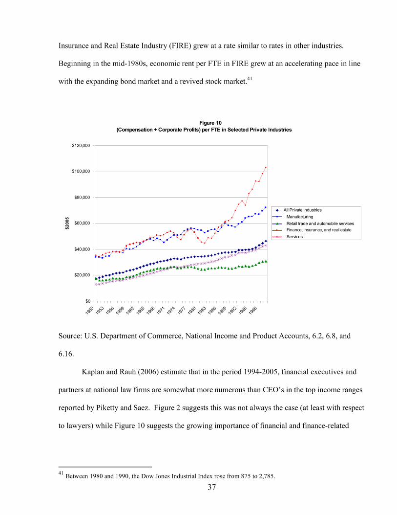


![Kato Kr-20h-l - Lift Chart[1]](https://static.documents.pub/doc/80x56/551534df497959071e8b4a9d/kato-kr-20h-l-lift-chart1.jpg)

