Inequality, fiscal policy, and business cycle … · Inequality, fiscal policy, and business cycle...

NBP Working Paper No. 253

Inequality, fiscal policy, and business cycle anomalies in emerging markets

Amanda Michaud, Jacek Rothert

Economic InstituteWarsaw, 2016

NBP Working Paper No. 253

Inequality, fiscal policy, and business cycle anomalies in emerging markets

Amanda Michaud, Jacek Rothert

Published by: Narodowy Bank Polski Education & Publishing Department ul. Świętokrzyska 11/21 00-919 Warszawa, Poland phone +48 22 185 23 35 www.nbp.pl

ISSN 2084-624X

© Copyright Narodowy Bank Polski, 2016

Amanda Michaud – Indiana University; contact: [email protected] Rothert – US Naval Academy; contact: [email protected]

Acknowledgments: We thank seminar participants at Indiana University, University of Western Ontario, Narodowy Bank Polski, 2015 Midwest Macroeconomics Meetings in Rochester, and the 2015 LACEA Annual Meeting. The views expressed are our own.

3NBP Working Paper No. 253

Contents1 Introduction 5

1.1 Literature 72 Empirical Regularities on the Composition of Fiscal Policy 9

3 Model 16

3.1 Production 163.2 Households 173.3 Cyclicality of fiscal policy 183.4 Solution method 18

4 Results 19

4.1 Quantitative implications of social transfers 194.2 Does the inequality matter? 21

5 Conclusions 23

A Equilibrium conditions 24

Narodowy Bank Polski4

Abstract

Abstract

Government expenditures are procyclical in emerging markets and countercyclical

in developed economies. We show this pattern is driven by differences in social trans-

fers: transfers are more countercyclical and make up a larger portion of spending in

developed economies. We use a small open economy model to study how much these

differences in fiscal policies can account for differences in business cycle characteristics

of emerging economies, particularly excess volatility of private consumption. We find

that ignoring disparate fiscal policy results in an overestimation of the persistence of

technology shocks in emerging markets relative to developed by 52%. We study how

this conclusion depends on differences in the extent and sources of inequality across

countries.

JEL Codes: E21, E32, E62, F41

Keywords: fiscal policy, emerging markets, trasnfers, inequality

2


Chapter 1

1 Introduction

We study the role disparate fiscal policies play in generating the business cycle anomalies

of emerging markets. Prior literature has documented that emerging markets experience

business cycles differently than developed economies. Consumption is more volatile relative

to output, real exchange rates depreciate during downturns, and the trade balance is strongly

counter-cyclical.1

A parallel literature has documented that the business cycle response of fiscal policy

in emerging markets is also distinctive.2 Total expenditures are procyclical in emerging

markets versus countercyclical in developed economies. This contrast is important because

fiscal procyclicality tends to amplify rather than mitigate underlying forces driving business

cycles. In this paper, we delve further into fiscal data and find this pattern holds for only one

key component of government expenditure: social transfers. Social transfers are acyclical

in emerging economies and countercyclical (correlation with GDP is -0.64) in developed

economies. This is important because social transfers are the largest expenditure category

in each country group. They comprise 36% of expenditures (12.3% of GDP) in developed

economies compared to 23% of expenditures (5.4% of GDP) in emerging economies. The

large differences in transfers trounce the minor differences in other categories such as Goods

Expenses, Fixed Capital, and Employee Compensation. Therefore, understanding the impact

of transfers is key for understanding the impact of overall fiscal policy on business cycle

outcomes.

We bridge these literatures by developing a small open economy business cycle model with

a role for government expenditure explicitly modeled as social transfers. The base of our

model is the workhorse small open economy model of Mendoza 1990. We generate emerging

market business cycle characteristics using a theory of trend shocks provided by Aguiar

and Gopinath. To the base model, we add heterogeneous households and a government.

Households differ in both their labor productivity and access to financial markets. The

government provides social transfers to poor households according to an exogenous process

replicating the level, standard deviation, and correlation with GDP of social benefits observed

1Key works in this field include: Mendoza (1995), Neumeyer and Perri (2005), Uribe and Yue (2006),

and Aguiar and Gopinath (2007).2See Alesina et al. (2008), Riascos and Vegh (2003), Talvi and Vegh (2005)

3


in the data. Social transfers are supported by taxes on rich households. Taxes are chosen

endogenously with the objective to smooth the tax burden overtime.3 Fiscal deficits are

covered by issuing bonds at the global interest rate and surpluses may be invested in the

same international market.4

We find that differences in fiscal policy go a long way in accounting for the contrasting

business cycle characteristics of emerging and developed economies. When we estimate the

model with realistic social transfers observed in the data, we find trend shocks account for

48% of the variation in TFP in emerging markets and 29% in developed. Re-estimating

the model with social transfers set to zero implies trend shocks account for 48% and 7% of

the variation of TFP in emerging and developed countries, respectively. We conclude that

ignoring redistribution provided by fiscal policy leads to a substantial overestimation in the

differences in the underlying TFP processes between emerging and developed economies.

This is an important result not only for understanding the risks nations face along the path

of economic growth, but also for understanding the stabilizing role of fiscal policy.

Emerging markets also feature higher income and wealth inequality than developed

economies above what can be accounted for by differences in social transfers. We explore how

the extent of inequality affects the macroeconomic impacts of social redistribution through

the channels of our model. First, we consider wealth inequality. We assume rich agents own

the capital stock and poor agents are hand-to-mouth consumers with no means of saving.

We find the smaller the share of rich agents in the economy, the smaller is the impact of

social benefits on cyclical properties of consumption and trade balance. Second, we consider

income inequality. We assume rich agents have higher efficiency units of labor than poor

agents resulting in a higher wage per unit of time worked. We find the larger the relative

labor income of rich agents, the larger is the effect of social transfers on cyclical properties

of consumption and trade balance. Thus, our results suggest the source of income inequality

3This assumption is motivated by the classical arguments of Barro (Barro (1979)), but may also be

interpreted as minimizing political and/or administrative costs necessary to change fiscal policy at high

frequency.4Sovereign default is obviously an important issue for emerging markets. However, the question we ask in

this paper does not require the explicit modeling of default. Instead, we can consider a partial equilibrium

interest rate on government bonds that depends on the current debt to GDP ratio. This captures the relevant

difference in constraints to tax smoothing in emerging and developed countries.

4

in the data. Social transfers are supported by taxes on rich households. Taxes are chosen

endogenously with the objective to smooth the tax burden overtime.3 Fiscal deficits are

covered by issuing bonds at the global interest rate and surpluses may be invested in the

same international market.4

We find that differences in fiscal policy go a long way in accounting for the contrasting

business cycle characteristics of emerging and developed economies. When we estimate the

model with realistic social transfers observed in the data, we find trend shocks account for

48% of the variation in TFP in emerging markets and 29% in developed. Re-estimating

the model with social transfers set to zero implies trend shocks account for 48% and 7% of

the variation of TFP in emerging and developed countries, respectively. We conclude that

ignoring redistribution provided by fiscal policy leads to a substantial overestimation in the

differences in the underlying TFP processes between emerging and developed economies.

This is an important result not only for understanding the risks nations face along the path

of economic growth, but also for understanding the stabilizing role of fiscal policy.

Emerging markets also feature higher income and wealth inequality than developed

economies above what can be accounted for by differences in social transfers. We explore how

the extent of inequality affects the macroeconomic impacts of social redistribution through

the channels of our model. First, we consider wealth inequality. We assume rich agents own

the capital stock and poor agents are hand-to-mouth consumers with no means of saving.

We find the smaller the share of rich agents in the economy, the smaller is the impact of

social benefits on cyclical properties of consumption and trade balance. Second, we consider

income inequality. We assume rich agents have higher efficiency units of labor than poor

agents resulting in a higher wage per unit of time worked. We find the larger the relative

labor income of rich agents, the larger is the effect of social transfers on cyclical properties

of consumption and trade balance. Thus, our results suggest the source of income inequality

3This assumption is motivated by the classical arguments of Barro (Barro (1979)), but may also be

interpreted as minimizing political and/or administrative costs necessary to change fiscal policy at high

frequency.4Sovereign default is obviously an important issue for emerging markets. However, the question we ask in

this paper does not require the explicit modeling of default. Instead, we can consider a partial equilibrium

interest rate on government bonds that depends on the current debt to GDP ratio. This captures the relevant

difference in constraints to tax smoothing in emerging and developed countries.

4

matters for business cycles.

1.1 Literature

Business cycles in emerging markets are different than in developed economies. Consumption

is more volatile than output and trade balance is strongly counter-cyclical. These two facts

are puzzling for the standard business cycle model of a small open economy. Numerous

suggested fluctuations in emerging markets were driven by fundamentally different sources

than in developed countries. Aguiar and Gopinath (2007) proposed productivity process in

emerging markets was different - emerging markets faced a more volatile shocks to growth

rate rather than level of productivity. Neumeyer and Perri (2005) and Uribe and Yue (2006)

emphasized the role of interest rate fluctuations and financial frictions. A number of follow-

up studies focused their efforts in evaluating the relative importance of the two sources

of fluctuations5, implicitly emphasizing the substantial difference between emerging and

developed economies. We show the differences between the two groups of countries may

have been over-estimated, once we take into account the behavior of fiscal policy, particularly

social transfers.

Ours is not the first paper to consider the role of fiscal policy in generating anomalies

of emerging markets business cycles. Gavin and Perotti (1997) first document the pattern

of procyclical fiscal policy in Latin America. Their work is followed by broader studies on

expenditures (Kaminsky et al. (2005)) and taxes (Ilzetzki and Vegh (2008)) reinforcing their

findings. Two complementary theoretical literatures are related to these empirical findings:

one seeking to understand the implication of fiscal policy in open economy business cycles

and one seeking to understand the fundamental cause of why these fiscal policies differ. Our

paper belongs to the first literature.6 The study of fiscal policy in open economy models was

included in early works. Backus et al. (1992) show that an increase in government spend-

ing causes a real exchange rate depreciation in the open economy neoclassical model. This

response has been shown to be counterfactual. For example, Ravn et al. (2007) document

5A non-exhausting list includes Chang and Fernandez (2013), Garcia-Cicco et al. (2010), Rothert (2012).6The second literature has provided theories related to limited access to international credit markets

(Cuadra et al. (2010),Riascos and Vegh (2003)) and political economy motives (Talvi and Vegh (2005),

Alesina et al. (2008)).

5


Introduction


1.1 Literature













social transfers.















5


1.1 Literature













social transfers.















5

that increases in government expenditure on goods deteriorates the trade balance and de-

preciates the real exchange rate. They provide a theory of deep habits where an increase in

government spending leads firms to lower domestic markups relative to foreign providing a

real exchange rate depreciation matching the data.

Our contribution to the quantitative theory literature is to explore how the composition

of government expenditures, not just the level, may reconcile outcomes in the neoclassical

open economy model with empirical observations. As such we depart from the standard

modelling assumptions as government expenditures as a sunk expense, or equivalently as

separable in the utility function of households. We also add agents who are heterogenous in

wealth and income into the analysis. These departures relate our paper to a third, emerging

literature on the calculation of government spending multipliers in models with heterogenous

agents. Most related is Brinca et al. (2014). They document a positive correlation between

fiscal multipliers and wealth inequality. They show a heterogenous agent neoclassical model

of incomplete markets can replicate this fact when government spending is modeled as social

security and appropriately calibrated. Ferriere and Navarro (2014) study the impact tax

progressivity on multipliers, but model expenditures as “thrown into the ocean”. Our work

is also distinct in considering an open economy setting.

Our empirical analysis of the IMF’s Government Finance Survey is an independent con-

tribution apart from our quantitative theory exercises. Changes in the survey overtime and

differences in reporting conventions across countries require significant cleaning of the dataset

to provide consistent measures of government expenditure at the categorical level. We devise

a detailed methodology to achieve this. We then merge the dataset with key variables from

other Macroeconomic datasets and compute a variety of statistics useful for studying issues

in growth, international macroeconomics, and political economy.

6


that increases in government expenditure on goods deteriorates the trade balance and de-

preciates the real exchange rate. They provide a theory of deep habits where an increase in

government spending leads firms to lower domestic markups relative to foreign providing a

real exchange rate depreciation matching the data.

Our contribution to the quantitative theory literature is to explore how the composition

of government expenditures, not just the level, may reconcile outcomes in the neoclassical

open economy model with empirical observations. As such we depart from the standard

modelling assumptions as government expenditures as a sunk expense, or equivalently as

separable in the utility function of households. We also add agents who are heterogenous in

wealth and income into the analysis. These departures relate our paper to a third, emerging

literature on the calculation of government spending multipliers in models with heterogenous

agents. Most related is Brinca et al. (2014). They document a positive correlation between

fiscal multipliers and wealth inequality. They show a heterogenous agent neoclassical model

of incomplete markets can replicate this fact when government spending is modeled as social

security and appropriately calibrated. Ferriere and Navarro (2014) study the impact tax

progressivity on multipliers, but model expenditures as “thrown into the ocean”. Our work

is also distinct in considering an open economy setting.

Our empirical analysis of the IMF’s Government Finance Survey is an independent con-

tribution apart from our quantitative theory exercises. Changes in the survey overtime and

differences in reporting conventions across countries require significant cleaning of the dataset

to provide consistent measures of government expenditure at the categorical level. We devise

a detailed methodology to achieve this. We then merge the dataset with key variables from

other Macroeconomic datasets and compute a variety of statistics useful for studying issues

in growth, international macroeconomics, and political economy.

6


Chapter 2

2 Empirical Regularities on the Composition of Fiscal

Policy

Government Finance Statistics Dataset 7 Our main dataset for fiscal variables is the

Government Finance Statistics Dataset (GFS) maintained by the International Monetary

Fund (IMF). The data collection began in 1972 with further guidelines established in 1986

intended to harmonize reporting of fiscal measures across countries. These guidelines have

subsequently been updated twice: once in 2001 and again in 2014. These changes have little

impact on our analysis with the exception of the expansion in the inclusion of nonmonetary

transactions. Most countries switched from cash accounting to accrual in the mid-1990s’

early 2000’s.

We use annual data. Higher frequency- monthly and quarterly data- are limited to a

smaller group of mostly developed countries.

Reported transactions are delineated by sub-sectors of the total Public Sector. Starting

from finest to coarsest, the sector-level reporting concepts we consider are:

1. Budgetary Central Government: a single unit encompassing financial activities of the

judiciary, legislature, ministries, president, and government agencies. It is funded by

the main operating budget of the nation, generally approved by the legislature. Items

not included in the budgetary central government statistics include extra-budgetary

units and transactions;8 and social security funds.

2. Central Government: the central government includes all transactions not operated

through a public corporation (ex: central bank and other financial institutions) that

are implemented at the national level (ie: not state or local governments). These

statistics may or may not include social security, depending on the country reporting.

Social security refers to social insurance schemes operated by a budget of assets and

liabilities separate from the general fund.

3. General Government: the sum of central, state, and local financial activities plus social

security. This does not include financial corporations.

7Information for this section comes from the 2014 GFS manual.8For example, units with revenue streams outside of the central budget, external grants received, etc.

7


Striation in the reporting of statistics by government level differs greatly across countries

and over time. This is a major difficulty in our analysis.

The transactions we analyze fall into the categories of revenues and expenses affecting

net worth. The specific breakdown is as follows.

• Revenue: transactions that increase net worth. These do not include transactions that

simply affect the composition of assets and liabilities in the balance sheet such as the

payments of loans or sale of financial assets.

1. Tax Revenue: compulsory, unrequited accounts receivable by the government.

Does not include, fines, penalties, and most social security contributions (as these

are requited). Taxe revenue can be further disaggregated into: (a) taxes on

income, profits and capital gains; (b) payroll taxes; (c) property taxes; (d) taxes

on goods and services; (e) taxes on international trades and transactions.

2. Social Contributions: revenue of social insurance schemes. May be voluntary or

compulsory.

3. Grants: transfers relievable that are not taxes, social contributions, or subsidies.

May come from domestic or international organizations and units.

4. Other: revenues not fitting in the aforementioned categories. Include: (a) prop-

erty income, (b) sales of goods and services, (c) fines, etc.

• Expense: transactions that decrease net worth. These do not include transactions that

simply affect the composition of assets and liabilities in the balance sheet.

1. Compensation of Employees: renumeration payable, both cash and in-kind, to

employees of the government unit. Includes contractors.

2. Use of Goods and Services: “value of goods and services used for the production of

market and nonmarket goods and services”. Includes consumption of fixed capital

and goods purchased by the government for direct distribution. Consumption of

fixed capital is also reported separately.

3. Interest: interest fees on liabilities generated by both financial and non-financial

services consumed by the government. Includes intra-government liabilities for

disaggregated units.

8


Empirical Regularities on the Composition of Fiscal Policy

Table 1: List of countriesEmerging Developed

Brazil Australia

Israel Austria

Malaysia Belgium

South Korea Canada

Peru Denmark

Slovakia Finland

South Africa Netherlands

Thailand New Zealand

Argentina Norway

Portugal

Spain

Sweden

Switzerland

4. Subsidies: unrequited transfers to enterprises based on production activities. In-

cludes implicit subsidies of central banks.

5. Social Benefits: current transfers receivable by household related to social risks.

These include: sickness, unemployment, retirement, housing, and education.

6. Other: transfers not otherwise classified, non-interest property expense, premiums

and fees on nonlife insurance schemes.

We consider an alternative measure of expenditure categorized by function: “social pro-

tection”. These expenditures are provided to individual persons and include (a) sickness and

disability; (b) old age and survivors; (c) family and children; (d) unemployment; (e) housing;

(f) social exclusion not otherwise classified.

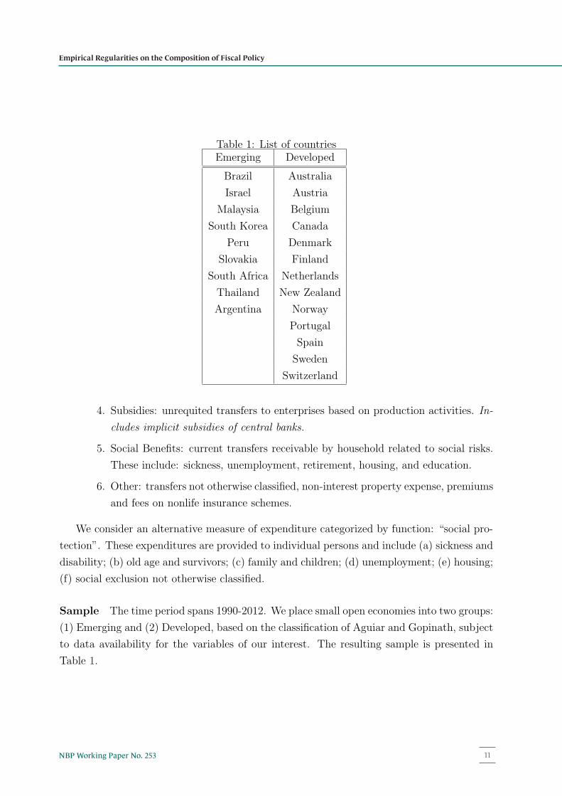
Sample The time period spans 1990-2012. We place small open economies into two groups:

(1) Emerging and (2) Developed, based on the classification of Aguiar and Gopinath, subject

to data availability for the variables of our interest. The resulting sample is presented in

Table 1.

9


Table 2: Macro StatisticsVariable Emerging Developed

std(y) 0.38 0.208

std(c)/std(y) 1.27 0.85

nx/gdp -0.016 0.013

corr(nx,gdp) -0.37 0.12

Constructing Consistent Measures of Revenues and Expenditures. Constructing

consistent measures of revenues and expenditures at the categorical level is non-trivial. The

first hurdle is that different countries implement fiscal policy through different government

bodies. For example, Brazil reports almost all social benefits are provided at the central

government level while subnational governments provide three-quarters of social benefits in

Denmark. This is a potential problem because the data are incomplete: some countries only

report spending at certain levels.9 The second hurdle is that some countries switch from

reporting cash to non-cash payments or switch the level at which they report payments:

general, central, of budgetary general. We handle each of these issues on a case-by-case basis.

In many cases the time-series remains smooth despite changes in the reported accounting

scheme. If these changes occur in the two years after the GFS survey is updated (1995-6,

2001-2) we use the two series as one consistent series. In cases where we observe general

government spending in ten or more years, we use this category as is. In cases where we only

observe central government spending in ten or more years, we continue to use the time series

if it is more than 85% of total government spending in the years where general government

spending is observed as well. Countries included in Aguiar and Gopinath (2007) that do not

meet either of these criteria are dropped (Mexico, Uruguay, etc.). We repeat this process for

each component of expenditures and revenues and their cash and non-cash reports.

Table 3 shows the following stylized facts about average expenses and revenues across the

country groups. Developed countries have higher mean total expenses and total revenues

over the sample. The difference in total expenses is driven almost entirely by the difference

in Social Benefits. Developed countries mean spending on social benefits is twice that of

emerging economies. Social benefits are also the largest expenditure category in each country

9The main issue is the exclusion of local governments for the emerging economies.

10



Table 3: Composition of Government Spending

Average Share of GDP

Variable Emerging Developed

Total Expenses 23.3 34.0

Compensation of Employees 5.05 4.86

Fixed Capital 1.2 1.0

Goods Expenses 4.03 3.19

Social Protection* 6.2 12.3

Social Benefits 5.42 12.30

Subsidies & Transfers 1.06 1.45

Interest 3.3 2.8

Other Expense 1.28 1.36

Total Revenue 23.2 33.6

Social contributions 3.16 8.11

Taxes 16.88 21.93

Grants 0.33 0.53

Other Revenue 3.2 4.0

Gini 47.5 29.5

*So-

cial Protection is calculated by a different accounting method catego-

rizing expenditure by function.

11


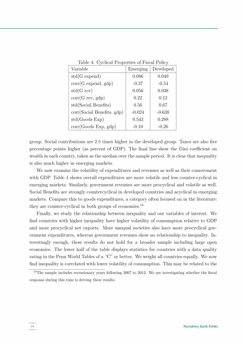
Table 4: Cyclical Properties of Fiscal Policy

Variable Emerging Developed

std(G expend) 0.086 0.049

corr(G expend, gdp) -0.37 -0.54

std(G rev) 0.056 0.038

corr(G rev, gdp) 0.22 0.12

std(Social Benefits) 0.56 0.67

corr(Social Benefits, gdp) -0.024 -0.638

std(Goods Exp) 0.543 0.288

corr(Goods Exp, gdp) -0.10 -0.26

group. Social contributions are 2.5 times higher in the developed group. Taxes are also five

percentage points higher (as percent of GDP). The final line show the Gini coefficient on

wealth in each country, taken as the median over the sample period. It is clear that inequality

is also much higher in emerging markets.

We now examine the volatility of expenditures and revenues as well as their comovement

with GDP. Table 4 shows overall expenditures are more volatile and less counter-cyclical in

emerging markets. Similarly, government revenues are more procyclical and volatile as well.

Social Benefits are strongly countercyclical in developed countries and acyclical in emerging

markets. Compare this to goods expenditures, a category often focused on in the literature:

they are counter-cyclical in both groups of economies.10

Finally, we study the relationship between inequality and our variables of interest. We

find countries with higher inequality have higher volatility of consumption relative to GDP

and more procyclical net exports. More unequal societies also have more procyclical gov-

ernment expenditures, whereas government revenues show no relationship to inequality. In-

terestingly enough, these results do not hold for a broader sample including large open

economies. The lower half of the table displays statistics for countries with a data quality

rating in the Penn World Tables of a “C” or better. We weight all countries equally. We now

find inequality is correlated with lower volatility of consumption. This may be related to the

10The sample includes recessionary years following 2007 to 2012. We are investigating whether the fiscal

response during this time is driving these results.

12



Table 5: Relationship to Inequality

Variable Pooled A&G Sample

corr(Gini , std(c)/std(y)) 0.214

corr(Gini , corr(NX,y)) 0.233

corr(Gini, std(y)) 0.52

corr(Gini, corr(G expend, GDP) 0.38

corr(Gini, corr(G rev, GDP)) -0.002

Variable PWT data quality better than “C”

corr(Gini , std(c)/std(y)) -0.25

corr(Gini , corr(NX,y)) -0.027

corr(Gini, std(y)) -0.013

corr(Gini, corr(G expend, GDP) -0.20

corr(Gini, corr(G rev, GDP)) -0.025

corr(Gini, corr(Social Ben, GDP) -0.355

fact that it also is correlated countercyclical expenditures and social benefits. This is rather

unsurprising as our data quality requirement trims the sample to mostly large, developed

economies.

13


Chapter 3

3 Model

In order to analyze the impact of inequality, and redistributive policies on business cycle

properties we build on workhorse real business cycle model of a small open, emerging econ-

omy (Mendoza (1991), Aguiar and Gopinath (2007) and Neumeyer and Perri (2005)). We

introduce inequality by considering two types of households: (R)ich and (P)oor. There is a

mass NR of rich households, and a mass NP of poor households. The difference between the

two is twofold. First, rich households have higher efficiency of labor input: efficiency of the

unit of labor of a poor household is 1, efficiency of the unit of labor of a rich household is

γ > 1. Second, only rich households can own physical capital.

3.1 Production

Aggregate production function is Cobb-Douglas with identical specification as in Aguiar and

Gopinath (2007):

Yt = eztKαt (ΓtLt)

1−α,

where zt is a temporary component of the log of total factor productivity (TFP), and Γt is

the trend component of the TFP. The inputs Kt, and Lt are aggregate capital stock and

aggregate labor respectively. The stochastic processes governing productivity are as follows:

zt = ρzzt−1 + �zt

Γt =Γt−1egt

gt =(1− ρg)μg + ρggt−1 + �gt

Aggregate capital stock is the sum of all the physical capital owned by rich households.

Aggregate labor input is the sum of effective labor inputs of the rich and the poor households:

Kt =NR · ktLt =NR · γ�Rt +NP �Pt

where kt is capital stock per rich household, �R and �P is labor supply per rich and poor

household, respectively.

14


Model

3.2 Households

The Rich A typical rich household solves the following utility maximization problem:

max∑t

βt

[cRt − χΓt−1

�Rt1+ν

1+ν

]1−σ

1− σ

subject to:

cRt + xt ≤wRt (1− τRt )�

Rt + rtkt−1 +Rt−1at−1 − at − κ

2(at − a)2

kt = (1− δ)kt−1 + xt − φ

2

(ktkt−1

− eμg

)2

kt−1

where the last term on the RHS of the budget constraint is a portfolio adjustment introduced

to ensure stationarity of the law of motion for assets in the linearized economy.

The Poor There is a mass NP of poor households. A typical poor household solves the

following utility maximization problem:

max∑t

βt

[cPt − χΓt−1

�Pt1+ν

1+ν

]1−σ

1− σ

subject to:

cPt ≤ wPt �

Pt + bt

where bt is the net social transfer from the government.

Government The government’s only expenditure is social benefits bt. We treat them as

an exogenous stochastic process, possibly correlated with other exogenous variables in the

model. Given the stochastic process for the social benefits {bt}, the government’s objective

is to minimize time variation in taxes, subject to the inter-temporal budget constraint. The

government solves the following problem:

min∑t

βt1

2TAX2

t

15


subject to:

TAXt =NR · τRt �Rt wRt

NP · bt +Rt−1Dt−1 =TAXt +Dt − 1

2κ�Dt − D · Γt−1

�2

log(bt)= (1− ρs)b+ ρs log bt−1 + �bt

The first constraint specifies the source of tax of revenues is labor tax imposed on rich

households. The second constraint is the government inter-temporal budget constraint. The

government has to finance exogenously given social transfers NP · bt and repay outstanding

debt. The two sources of revenue to cover this expenditure are tax revenues TAXt and

newly issued debt Dt. The last term on the RHS is a quadratic adjustment cost introduced

to ensure stationarity of the law of motion for government debt in the linearized economy.

Finally, the last equation specifies the stochastic process for social transfers.

3.3 Cyclicality of fiscal policy

Cyclicality of fiscal policy is introduced exogenously by specifying a joint stochastic process

for the vector of shocks: [�zt , �gt , �

sbt ]. The stochastic process takes the following form:

⎛⎜⎝

�zt

�gt

�sbt

⎞⎟⎠ ∼ N (0,Σ)

where the variance co-variance matrix Σ is given by:

Σ =

⎛⎜⎝

σ2z 0 σz,sb

0 σ2g σg,sb

σz,sb σg,sb σ2sb

⎞⎟⎠

The cyclicality of social transfers will be driven by two parameters: σz,sb, and σg,sb.

3.4 Solution method

We solve the model with local methods by linearizing the equilibrium conditions around

the non-stochastic steady-state. We use Dynare for this step. Equilibrium conditions are

described in the appendix.

16


Chapter 4

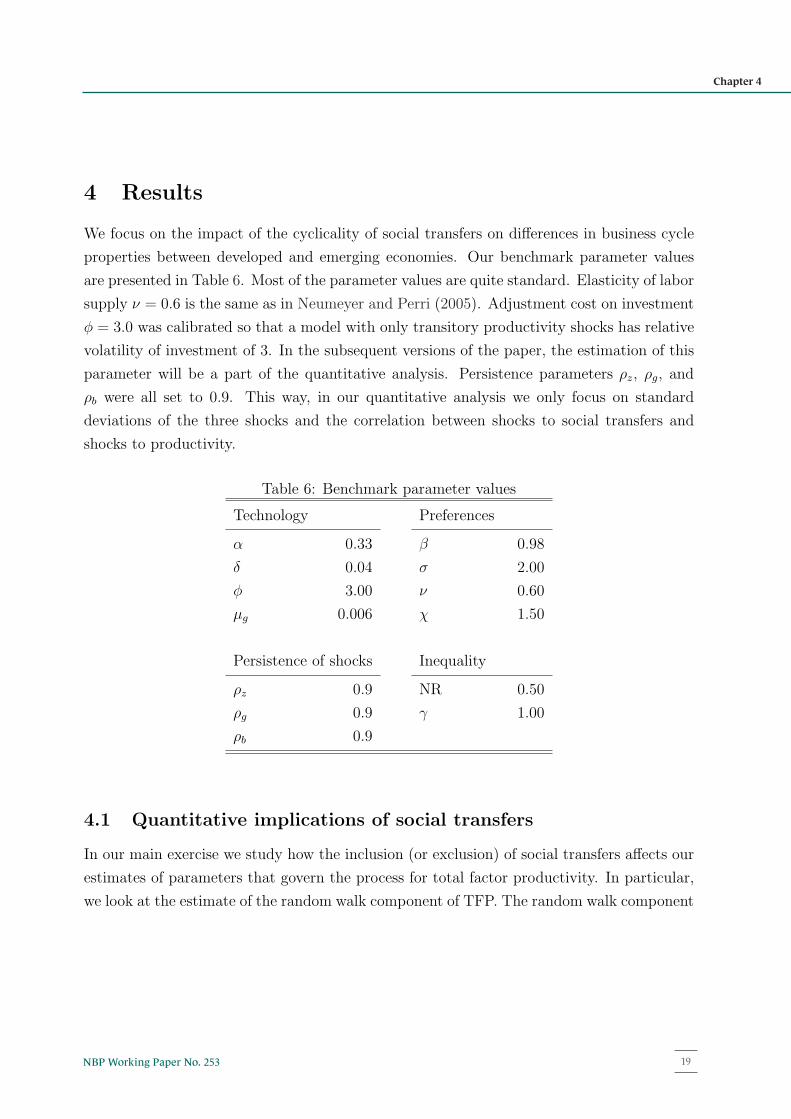
4 Results

We focus on the impact of the cyclicality of social transfers on differences in business cycle

properties between developed and emerging economies. Our benchmark parameter values

are presented in Table 6. Most of the parameter values are quite standard. Elasticity of labor

supply ν = 0.6 is the same as in Neumeyer and Perri (2005). Adjustment cost on investment

φ = 3.0 was calibrated so that a model with only transitory productivity shocks has relative

volatility of investment of 3. In the subsequent versions of the paper, the estimation of this

parameter will be a part of the quantitative analysis. Persistence parameters ρz, ρg, and

ρb were all set to 0.9. This way, in our quantitative analysis we only focus on standard

deviations of the three shocks and the correlation between shocks to social transfers and

shocks to productivity.

Table 6: Benchmark parameter values

Technology Preferences

α 0.33 β 0.98

δ 0.04 σ 2.00

φ 3.00 ν 0.60

μg 0.006 χ 1.50

Persistence of shocks Inequality

ρz 0.9 NR 0.50

ρg 0.9 γ 1.00

ρb 0.9

4.1 Quantitative implications of social transfers

In our main exercise we study how the inclusion (or exclusion) of social transfers affects our

estimates of parameters that govern the process for total factor productivity. In particular,

we look at the estimate of the random walk component of TFP. The random walk component

17


Table 7: Results

Model w/o transfers Model w/ transfers

Emerging Developed Difference Emerging Developed Difference

σz 0.145 0.091 0.054 0.145 0.085 0.060

σg 0.093 0.017 0.076 0.093 0.036 0.057

σ2z

1−ρ2z

0.763 0.479 0.284 0.763 0.447 0.316σ2g

1−ρ2g

0.489 0.089 0.400 0.489 0.189 0.300

σb N/A N/A N/A 0.550 0.650 -0.100

corr(�z, �b) N/A N/A N/A -0.020 -0.530 0.510

Random walk

component of TFP 48% 7% 41% 48% 29% 19%

of TFP is calculated using the formula (14) in Aguiar and Gopinath (2007):

RW =(1− α)2σ2

g/(1− ρ2g)

[2/(1 + ρz)]σ2z + [(1− α)2σ2

g/(1− ρ2g)]

We first consider a restricted model with σb = 0. In this restricted model we estimate two

parameters—σz, and σg—by matching two empirical moments—standard deviation of GDP,

and the relative standard deviation of consumption. Then, we drop the restriction that

σb = 0, and we also allow for σz,b �= 0, and for σg,b �= 0 (for simplicity we only impose

restriction that σg,b = σz,b, i.e. transfers respond identically to transitory and permanent

productivity shocks). In that estimation we use additional two moments—standard deviation

of social benefits, and correlation between GDP and social benefits. In each case we focus

on the difference between emerging and developed in the importance of the random walk

component of TFP. Our results are summarized in Table 7.

In the model without social transfers about 48% of the TFP variance in emerging markets

is accounted for by trend shocks. In developed countries this number is only 7%. For

comparison, Chang and Fernandez (2013) estimate the random walk component in emerging

markets to be 28%, Rothert (2012) estimates it to be 61%, while Aguiar and Gopinath (2007)

estimates it to be 96%11.

11We only provide these numbers for reference, without drawing any conclusions. Our model features

18


Results

When we include social transfers and estimate their cyclical behavior to mimic the one

in the data, the difference between emerging and developed countries shrinks dramatically.

Since transfers are largely acyclical in emerging economies, our estimates of σz and σg for

this group remains essentially the same. However, the strong counter-cyclicality and high

volatility of social transfers in developed countries has a big impact on our estimates of the

productivity process in that group. We now estimate that as much as 29% of the TFP

variance in developed countries is accounted for by trend shocks. This is only 19 percentage

points difference from emerging markets, comparing to 41 percentage points difference if we

do not take into account the cyclical behavior of social benefits.

4.2 Does the inequality matter?

We explore the impact of inequality by changing two parameters: the fraction of population

that owns capital (NR = 0.35), and the relative labor productivity of capital owners (γ =

1.5). In each case we estimate the model without and with social transfers, and see how the

inclusion of transfers affects the difference between emerging and developed countries. Our

preliminary results suggest the, given the cyclicality of transfers, the impact of inequality is

not very large.

Table 8: Random walk component of TFP - the role of inequality

Model w/o transfers Model w/ transfers

Emerging Developed Difference Emerging Developed Difference

Benchmark 48% 7% 41% 48% 29% 19%

NR = 0.35 45% 7% 38% 44% 23% 21%

γ = 1.5 42% 4% 38% 42% 29% 13%

When changes in inequality come from changes in relative labor productivity, the im-

heterogenous households, where only the rich own capital stock, and only the rich are allowed to borrow or

lend. Naturally, our benchmark estimates will differ.

19


pact of social transfers on qualitative features of business cycles is stronger. For developed

countries, taking into account social benefits, increases the estimate of the random walk

component by 25 percentage points (comparing to the increase by 22 percentage points with

γ = 1). When changes in inequality come from changes in capital ownership, the result is

opposite. For developed countries, taking into account social benefits, increases the estimate

of the random walk component by 16 percentage points (comparing to the increase by 22

percentage points with NR = 0.5).

20


Chapter 5

5 Conclusions

We studied the role disparate fiscal policies play in generating the business cycle anomalies

of emerging markets. We first documented substantial differences in the business cycle

properties of various components of fiscal policy in developed and emerging economies. In

particular, we showed the key difference between the two groups of countries is in the cyclical

behavior of social transfers.

We then studied how these differences affect our conclusions about differences in the

sources of business cycle fluctuations in emerging vs. developed countries. We considered

a workhorse, real business cycle model of a small open economy with heterogenous house-

holds, in order to account for differences in inequality and to study redistributive policies.

Accounting for social transfers drastically reduces the estimated differences between emerg-

ing and developed economies. Ignoring cyclicality of social transfers leads us to believe the

random walk component of total factor productivity in emerging economies is 7 times more

important than in developed countries. Taking that cyclicality into account, reduces that

ratio to 2.

Overall, our results indicate the fundamental differences between emerging and developed

countries may be exaggerated if one does not take into account differences in the behavior

of fiscal policy.

21


References

References

Aguiar, M. and G. Gopinath (2007): “Emerging Market Business Cycles: The Cycle Is

the Trend,” Journal of Political Economy, 115.

Alesina, A., F. R. Campante, and G. Tabellini (2008): “Why is fiscal policy often

procyclical?” Journal of the european economic association, 6, 1006–1036.

Backus, D., P. J. Kehoe, and F. E. Kydland (1992): “Dynamics of the Trade Balance

and the Terms of Trade: The S-curve,” Tech. rep., National Bureau of Economic Research.

Barro, R. J. (1979): “On the Determination of the Public Debt,” Journal of Political

Economy, 87, 940–71.

Brinca, P. S., H. A. Holter, P. Krusell, and L. Malafry (2014): “Fiscal Multi-

pliers in the 21st Century,” Robert Schuman Centre for Advanced Studies Research Paper.

Chang, R. and A. Fernandez (2013): “On the sources of aggregate fluctuations in

emerging economies,” International Economic Review, 54, 1265–1293.

Cuadra, G., J. M. Sanchez, and H. Sapriza (2010): “Fiscal policy and default risk in

emerging markets,” Review of Economic Dynamics, 13, 452–469.

Ferriere, A. and G. Navarro (2014): “The Heterogeneous Effects of Government

Spending: It’s All About Taxes,” .

Garcia-Cicco, J., R. Pancrazi, and M. Uribe (2010): “Real Business Cycles in Emerg-

ing Countries?” American Economic Review, 100, 2510–31.

Gavin, M. and R. Perotti (1997): “Fiscal policy in latin america,” in NBER Macroeco-

nomics Annual 1997, Volume 12, Mit Press, 11–72.

Ilzetzki, E. and C. A. Vegh (2008): “Procyclical fiscal policy in developing countries:

Truth or fiction?” Tech. rep., National Bureau of Economic Research.

Kaminsky, G. L., C. M. Reinhart, and C. A. Vegh (2005): “When it rains, it pours:

procyclical capital flows and macroeconomic policies,” in NBER Macroeconomics Annual

2004, Volume 19, MIT Press, 11–82.

22


References

Mendoza, E. G. (1991): “Real Business Cycles in a Small Open Economy,” American

Economic Review, 81, 797–818.

——— (1995): “The terms of trade, the real exchange rate, and economic fluctuations,”

International Economic Review, 101–137.

Neumeyer, P. A. and F. Perri (2005): “Business cycles in emerging economies: the role

of interest rates,” Journal of Monetary Economics, 52, 345–380.

Ravn, M. O., S. Schmitt-Grohe, and M. Uribe (2007): “Explaining the effects of

government spending shocks on consumption and the real exchange rate,” Tech. rep.,

National Bureau of Economic Research.

Riascos, A. and C. A. Vegh (2003): “Procyclical government spending in developing

countries: The role of capital market imperfections,” unpublished (Washington: Interna-

tional Monetary Fund).

Rothert, J. A. (2012): “Productivity or Demand: Identifying Sources of Fluctuations in

Emerging Markets,” Society for Economic Dynamics 2012 Meeting Papers.

Talvi, E. and C. A. Vegh (2005): “Tax base variability and procyclical fiscal policy in

developing countries,” Journal of Development economics, 78, 156–190.

Uribe, M. and V. Z. Yue (2006): “Country spreads and emerging countries: Who drives

whom?” Journal of international Economics, 69, 6–36.

23


Appendices

Appendices

A Equilibrium conditions

Since our model features a stochastic trend, we need to make the model stationary. We

do so, by dividing all the variables containing the trend by Γt−1. The resulting equilibrium

conditions are as follows.

Production function:

yt = ezt(NR · kt−1)α [egtLt]

1−α

where Lt =(NRγ · �Pt +NP · �Pt

).

Capital law of motion:

egtkt = (1− δ)kt−1 + xt − φ

2

(egt

ktkt−1

− eμg

)2

kt−1

Resource constraint:

NP cPt +NRcTt +NRxt +NXt = yt

Consumption leisure trade-off:

−U�,t/Uc,t = wit, i = R,P

where

wPt =(1− α)Yt/Lt

wRt = γwP

t

Government budget constraint:

NP · bt +Rt−1dt−1 = TAXt + egtdt − 1

2κ(dt − d

)2

Poor household’s budget constraint:

cPt = ePt �Pt + bt

24


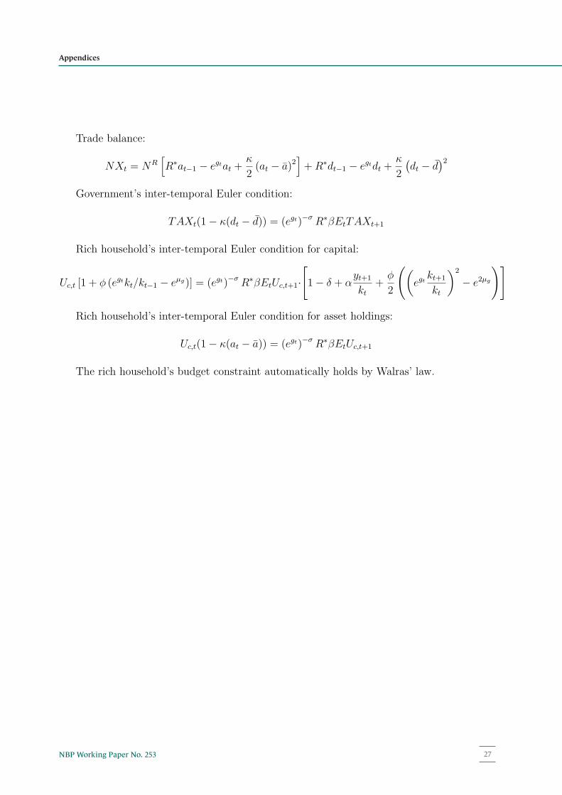
Appendices

Trade balance:

NXt = NR[R∗at−1 − egtat +

κ

2(at − a)2

]+R∗dt−1 − egtdt +

κ

2

(dt − d

)2

Government’s inter-temporal Euler condition:

TAXt(1− κ(dt − d)) = (egt)−σ R∗βEtTAXt+1

Rich household’s inter-temporal Euler condition for capital:

Uc,t [1 + φ (egtkt/kt−1 − eμg)] = (egt)−σ R∗βEtUc,t+1·[1− δ + α

yt+1

kt+

φ

2

((egt

kt+1

kt

)2

− e2μg

)]

Rich household’s inter-temporal Euler condition for asset holdings:

Uc,t(1− κ(at − a)) = (egt)−σ R∗βEtUc,t+1

The rich household’s budget constraint automatically holds by Walras’ law.

25

www.nbp.pl

Date post:	05-Sep-2018
Category:	Documents
Upload:	doandien
View:	215 times
Download:	0 times

Inequality, fiscal policy, and business cycle … · Inequality, fiscal policy, and business cycle...

Documents