Unclassified ECO/WKP(2016)65 Organisation de Coopération et de Développement Économiques Organisation for Economic Co-operation and Development 17-Nov-2016 ___________________________________________________________________________________________ _____________ English - Or. English ECONOMICS DEPARTMENT INEQUALITY IN DENMARK THROUGH THE LOOKING GLASS ECONOMICS DEPARTMENT WORKING PAPERS No. 1341 By Orsetta Causa, Mikkel Hermansen, Nicolas Ruiz, Caroline Klein and Zuzana Smidova OECD Working Papers should not be reported as representing the official views of the OECD or of its member countries. The opinions expressed and arguments employed are those of the author(s). Authorised for publication by Christian Kastrop, Director, Policy Studies Branch, Economics Department. All Economics Department Working Papers are available at www.oecd.org/eco/workingpapers JT03405564 Complete document available on OLIS in its original format This document and any map included herein are without prejudice to the status of or sovereignty over any territory, to the delimitation of international frontiers and boundaries and to the name of any territory, city or area. ECO/WKP(2016)65 Unclassified English - Or. English
Transcript
Unclassified ECO/WKP(2016)65 Organisation de Coopération et de Développement Économiques Organisation for Economic Co-operation and Development 17-Nov-2016
This paper delivers a broad assessment of income inequality in Denmark. As a necessary preamble to
provide a basis for discussion, we start by contrasting Danish official inequality measures with those
gathered by the OECD in an international context. We show that differences between these two sources are
fully explained by differences in methodological choices. We then go beyond synthetic measures of
inequality to deliver a granular assessment of income distribution and of the distributional impact of taxes
and transfers; and on this basis we compare Denmark to other OECD countries. This approach is then used
to quantify the distributional impact of some growth-enhancing reforms undertaken or recommended for
Denmark, based on empirical evidence across OECD countries. Finally, we take a forward looking stance
by discussing global forces shaping the rise in inequality, in particular skill-biased technological change
and deliver a tentative scenario for Denmark in the wider OECD context.
JEL codes: O15; D31; H23; E61
Keywords: income distribution, inequality, general means, structural policies
************************
Les inégalités au Danemark : mesures, évolutions et impacts de réformes récentes
Ce document de travail fournit une évaluation générale de l'inégalité de revenu au Danemark. En
préambule afin de fournir une base aux discussions, ce papier commence par une comparaison entre les
mesures d'inégalité officielles danoises et celles recueillies par l'OCDE dans un contexte international. Il
est montré que les différences entre ces deux sources sont expliquées principalement par des différences de
choix méthodologiques. Ensuite, au-delà des mesures synthétiques de l'inégalité, le document fournit une
évaluation granulaire des inégalités et de l'impact redistributif des impôts et des transferts au Danemark,
dans une perspective internationale. Cette approche est ensuite utilisée pour quantifier l'impact redistributif
de certaines réformes pro-croissance. Enfin, les potentielles évolutions futures des inégalités au Danemark
sont discutées, au regard des récentes tendances mondiales, en particulier le changement technologique et
son influence sur la demande de compétences.
Codes JEL: O15; D31; H23; E61
Mots clés: inégalité, moyennes généralisées, politiques structurelles
ECO/WKP(2016)65
4
TABLE OF CONTENTS
1. Introduction and key findings ............................................................................................................... 6 2. Measuring income inequality in Denmark............................................................................................ 7
Denmark is among the most equal countries in the OECD … ................................................................. 7 …but different measurement can lead to different assessment ................................................................ 9 Key differences in data selection and transformation ............................................................................ 11 Key differences in income definition ..................................................................................................... 12 Summarising the overall impact of differences in inequality measurement .......................................... 17 Inequality in the tails: top incomes and poverty ..................................................................................... 20 Going further: the OECD granular approach to income inequality........................................................ 23 Wrapping-up inequality developments and introducing the sources of rising inequality ...................... 32
3. Estimating the impact of selected policy reforms ............................................................................... 32 4. Looking forward: scenario analysis on future inequality developments ............................................ 39
The Tinbergen model of earnings inequality ......................................................................................... 39 Baseline scenario .................................................................................................................................... 41 Alternative scenario ................................................................................................................................ 44
5. Conclusions and future research ......................................................................................................... 44
Table 1. Differences in data selection and transformation .................................................................. 11 Table 2. Differences in household income definition .......................................................................... 13 Table A.1 Differences in data selection and transformation and income definition ............................. 49
Figures
Figure 1. Income inequality in Denmark is among the lowest across OECD countries ........................ 8
Figure 2. National sources report a higher level of inequality in Denmark since mid-2000s than the
Figure 16. Effects of a reduction in regulation in network industries on household disposable incomes .... 38
Figure 17. Effects of an increase in value added of finance on household disposable incomes ............ 39
Figure 18. Effects of an increase in value added of finance on household disposable incomes ............ 42 Figure 19. Increase in earnings inequality (D9/D1) if employment protection, union coverage, tax
wedges and PMR are set equal to the lowest levels in the sample ....................................... 43 Figure A1. Mean disposable income deciles ........................................................................................... 50
Boxes
Box 1. Owner-occupied housing services in Danish income statistics ..................................................... 15 Box 2. Rising capital incomes and inequality increase in Denmark .......................................................... 19 Box 3. The general mean approach ............................................................................................................ 23 Box 4. OECD framework on the impact of structural policies across the income distribution ................. 33
ECO/WKP(2016)65
6
INEQUALITY IN DENMARK THROUGH THE LOOKING GLASS
Orsetta Causa, Mikkel Hermansen, Nicolas Ruiz, Caroline Klein and Zuzana Smidova1
1. Introduction and key findings
1. The Danish society is increasingly concerned about increasing income inequality and its link
with growth. Although Denmark is one of the least unequal countries in the world, it has not been immune
from the recent global rise in income inequality. Indeed, the Gini coefficient (a common measure of
income inequality, with a score of 0 if everybody has identical incomes and 100 if all income goes to one
person) rose by the same proportion as the OECD average, i.e. by almost 3 points over the past three
decades. Also, the recovery from the recent financial crisis has been sluggish and late in Denmark and
2015 GDP remains below the pre-crisis level. The economy is expected to grow at just below 2% in the
coming years, but the prospects are fairly uncertain. Moreover, though GDP growth has benefitted
households fairly equally across the income distribution during mid-1980s to mid-2000s, it has recently
tended to benefit relatively more the upper-half of the distribution. At the same time, the re-distributive
features of the welfare system have been weakened.
2. This paper delivers an assessment of income distribution in Denmark in a comparative
perspective with respect to high-income OECD countries. A first step is to clarify how inequality is being
measured, and this is one of the core issues addressed in this paper. There is no single way to measure
inequality, even if there are fundamental theoretical and empirical rules to be respected. Nevertheless,
different legitimate measurement choices may lead to different assessments. In particular, measurement
criteria used in an international comparative perspective are likely to not coincide with those used in a
national context. We document this issue through the lenses of the Danish (national) approach to inequality
measurement, which we compare to the OECD (international) approach. Against this background and with
a good understanding of measurement issues, we provide a comprehensive assessment of income
inequality in Denmark, going beyond synthetic indicators such as the Gini coefficient, hence covering the
wide spectrum of the income distribution. We then use this approach to quantify the distributional impact
of some growth-enhancing reforms undertaken over the last decades in Denmark. We finally provide a
forward-looking scenario on long-term income inequality challenges for Denmark and the rest of the
OECD.
3. Main findings can be summarised as follows:
Assessing income inequality depends on how income inequality is being measured:
o The differences between the Gini coefficient published by the Danish government and that
published by the OECD can be fully explained by differences in measurement approach,
1. The authors are members of the Economics Department of the OECD. This paper was produced as a
background paper for a seminar on income inequality in Denmark on November 5th
, 2015 at Copenhagen
Economics. The authors would like to thank Helge Sigurd Næss-Schmidt (Copenhagen Economics) for
initiating and hosting the seminar. They would also like to thank Economics Department colleagues Alain
de Serres, Christian Kastrop, Andreas Wörgötter, seminar participants at Copenhagen Economics, and
colleagues from the Directorate for Employment, Labour and Social Affairs and the Statistics Directorate
for useful comments and suggestions. They also thank Caroline Abettan for editorial assistance.
ECO/WKP(2016)65
7
such as the household definition and the treatment of the housing services that
homeowners provide to themselves.
o Assessing inequality on the basis of synthetic measures such as the Gini coefficient is
bound to deliver an incomplete picture of income inequality, one that heavily depends on
some part of the distribution. The OECD has developed a more granular approach to
inequality allowing for capturing every part of the income distribution, hence to
identifying the sources of inequality, at a given moment and over time. This is achieved by
the use of general means.
Denmark has one of the lowest degrees of income inequality in the world. This conclusion holds
for a range of inequality measures from the Gini coefficient to tail incomes as well as the granular
approach.
Income inequality has been increasing around the same pace as the OECD average. This was
driven by a global trend towards increased earnings dispersion, but also rising capital incomes as
well as changes in household structure.
Tentative analysis based on cross-country time series for all OECD countries suggests that some of
the growth-enhancing structural reforms implemented in Denmark over the recent decades may
have contributed to increase inequality in household disposable income. Such is the case of the
reduction in unemployment benefits generosity but also of financial deregulation, in particular due
to the rise in household indebtedness.
Nevertheless, the main long-term driver of increasing inequality across developed countries has
been skill-biased technological change. This global trend is likely to continue, and the OECD 50-
Year Global Scenario suggests that, absent policy response, the level of earnings inequality in
Denmark could reach, by 2060, that prevailing today in the United Kingdom.
4. This paper is structured as follows. Section 2 delivers a detailed discussion on issues associated
with income inequality measurement, focusing on Denmark. Section 3 delivers a preliminary assessment of
the distributional impact of growth-enhancing reforms implemented over the recent decades in Denmark,
based on a new empirical framework developed at the OECD. Section 4 takes a forward-looking approach
and presents long-term scenarios for earnings inequality in Denmark, in a cross-country comparative
perspective, based on OECD long-term projections. Section 5 proposes some potential options for future
research, on the basis of the issues raised by the paper.
2. Measuring income inequality in Denmark
Denmark is among the most equal countries in the OECD …
5. Denmark scores well on many dimensions of well-being. It is ranked as the happiest nation in the
world (Helliwell et al., 2016). It is also ranked among the most equal countries. According to OECD
sources, the level of household disposable income inequality prevailing in Denmark, as measured by the
Gini coefficient is the lowest across the OECD (Figure 1, Panel A). The Gini coefficient comes out at 24.9
in 2012, well below the OECD average of 31.5, while not far from other Nordic countries. Alternative
measures of inequality barely modify this conclusion.2
2. Measures like the P90/P10, S80/S20, and the Palma ratio (the ratio between the income share of the top
10% and the bottom 40%) result in a similar ranking of Denmark as one of the most equal countries in the
OECD (OECD, 2015a).
ECO/WKP(2016)65
8
Figure 1. Income inequality in Denmark is among the lowest across OECD countries
Gini coefficient, 2012
Note: Data refer to 2014 for Hungary; 2013 for Finland, Israel, Korea, Netherlands and the United States; 2011 for Canada and Chile; 2009 for Japan and 2012 for the rest.
Source: OECD Income Distribution Database.
0
10
20
30
40
50
60
DN
K
SV
N
SV
K
NO
R
CZ
E
ISL
FIN
BE
L
SW
E
AU
T
NLD
CH
E
HU
N
DE
U
PO
L
LUX
KO
R
IRL
FR
A
OE…
CA
N
AU
S
ITA
NZ
L
ES
P
JPN
PR
T
ES
T
GR
C
GB
R
ISR
US
A
TU
R
ME
X
CH
L
A. Disposable income for total population
0
10
20
30
40
50
60
KO
R
CH
E
ISL
SV
K
NLD
SW
E
NO
R
CZ
E
DN
K
HU
N
JPN
DE
U
TU
R
CA
N
AU
S
SV
N
NZ
L
BE
L
OE…
FIN
ISR
PO
L
ES
T
AU
T
ITA
LUX
FR
A
ES
P
ME
X
US
A
PR
T
GR
C
CH
L
IRL
B. Market income for working age population (age 18-65)
0
10
20
30
40
50
60
SV
K
CZ
E
DN
K
NO
R
HU
N
BE
L
NLD IS
L
PO
L
FIN
ES
T
SV
N
GR
C
AU
T
DE
U
CA
N
SW
E
LUX
IRL
ES
P
OE…
CH
E
ITA
FR
A
NZ
L
AU
S
GB
R
PR
T
JPN
TU
R
ISR
US
A
KO
R
CH
L
ME
XC. Disposable income for retirement age population (above age 65)
ECO/WKP(2016)65
9
6. Such low level of inequality can be partly explained by the breadth of the redistributive system in
Denmark, as the strong welfare system plays a crucial role in mitigating the impact of market income
inequality on disposable income inequality (i.e. market income after taxes and transfers). That said, even
the level of market income inequality is relatively low compared to many OECD countries. The Gini
coefficient for market income inequality in the working age population stands at 39.6 (Figure 1, Panel B),
the 9th lowest in the OECD. Part of the taxes paid by the working age population are used to finance the
public pension scheme, which is characterised by a relatively high replacement rate for pensioners with no
or limited savings (OECD, 2013a). This results in a very equal income distribution among the retirement
age population, the 3th lowest in the OECD (Figure 1, Panel C).
…but different measurement can lead to different assessment
7. The assessment of income inequality can change depending on measurement factors. OECD
official figures presented above are based on the OECD Income Distribution Database (IDD), a secondary
data-set established to benchmark and monitor income distribution across OECD countries.3 It gathers a
number of standardized indicators available under the form of semi-aggregated tabulations based on
national sources, deemed to be most representative in each country. The method of data collection aims to
maximize international comparability as well as inter-temporal consistency of the data. This is achieved
through a common set of protocols and statistical conventions based on internationally agreed statistical
standards.4
8. International protocols and conventions tend to discard specific differences in measurement
which cannot be transposed in an international context, but may matter at the country level. International
standards generally set the rules for the choice of the unit of analysis (individual vs households), for how to
compare incomes from households of different size (equivalence scale), and, most critically, for the choice
of the income concept. In this respect, the income concept should account for a variety of different income
sources (e.g. labour and capital income, including from self-employment), while others should be excluded
(e.g. capital gains and losses from financial and non-financial assets which are not considered as part of
income but as such changes in net worth). In practice, the IDD cannot comply with the most
comprehensive definition of household income, mainly because the underlying data sources do not provide
all the necessary information, but also because some available elements have to be excluded due to poor
cross-country comparability. Such is the case of imputed rents from owner-occupied dwellings. As a result,
official figures on income inequality published by national sources often differ from those of the IDD.
9. The national statistical agency, Statistics Denmark, and the Danish government produce their
own measures of inequality.5 Their measures do not follow international standards but are customized to
the data source available. As a result, the Gini coefficients reported by the two national institutions differ
from the OECD numbers (Figure 2, Panel A).
3. The data cover the period mid-80s/2013. The database is currently being updated annually but with a 2-3
year lag for most countries.
4. See the Canberra Group Handbook (UNECE, 2011) and OECD (2013b).
5. In the following the term “the Danish government” is used since different ministries have been responsible
of inequality assessments during recent years. Previously the Ministry of Finance was in charge, while the
most recent publications are from the Ministry of Economic Affairs and the Interior (2015a). After the
recent election this ministry has been closed and activities moved to other ministries.
ECO/WKP(2016)65
10
Figure 2. National sources report a higher level of inequality in Denmark since mid-2000s than the OECD
Note: Household disposable income for the total population.
Source: Ministry of Economic Affairs and the Interior (2015a), OECD Income Distribution Database, Statistics Denmark (2015a).
10. Remarkably, national measures also differ among themselves, by almost 2 percentage points.
According to Statistics Denmark, the Gini coefficient for household disposable income was 27.4 in 2012,
whereas the Danish government reports a level of 25.7. Both numbers exceed those reported by the OECD,
but the ranking of the three institutions has been the same since the mid-2000s. As a result year-on-year
changes are highly correlated (Figure 2, Panel B), although the OECD figures seem to deviate between
2007 and 2009.
11. The differences between these measures derive mainly from two factors: i) data selection and
transformation and ii) income definition. In what follows, the main focus will be on the difference between
the Danish government and the OECD measurement approaches.6 The idea is to identify and try to
6. See the appendix for a detailed table summarizing the differences vis-à-vis Statistics Denmark and an
illustration of the overall implications for gauging income distributions.
10
15
20
25
30
35
40
1985 1990 1995 2000 2005 2010
A. Gini coefficient in levels
OECD Danish government Statistics Denmark
Corr(OECD, Danish gov): 0.95
Corr(OECD, Statistics Denmark): 0.88
Corr(Danish gov, Statistics Denmark): 0.98
-1.5
-1
-0.5
0
0.5
1
1.5
2
2006 2007 2008 2009 2010 2011 2012 2013
Percentage points
B. Year-on-year changes
OECD Danish government Statistics Denmark
Corr(OECD, Danish gov): 0.75
Corr(OECD, Statistics Denmark): 0.56
Corr(Danish gov, Statistics Denmark): 0.93
ECO/WKP(2016)65
11
quantify the sources of the difference between associated Gini coefficients. This can be achieved because
the IDD is based on the same Danish dataset used for official figures: the data are treated differently, as
will be analysed in this section (see also OECD, 2012a).7 The Danish figures are always constructed from
national register data covering the full population and based on detailed information from tax records. This
reflects the very high standard of the Danish statistical apparatus – almost unique in the OECD in terms of
coverage, depth, accuracy and availability. Such high data quality makes Denmark particularly well suited
for an in-depth analysis of inequality measurement.
Key differences in data selection and transformation
12. In terms of data selection and transformation, the Danish government and the OECD approach
differ mainly in three ways (Table 1). This is because the OECD definition needs to be applied on a large
set of countries, which necessitates minimising the complexity of the figures requested from countries.
Table 1. Differences in data selection and transformation
OECD Implication for
inequality measure1
Danish government
Household definition
Individual or group of persons who live together under the same housing arrangement and who combine to provide themselves with food and possible other essentials of living.
<
The family is the unit of analysis, i.e. for two persons to form a household they have to be in a relationship. A family is an individual or couple living together with or without children. More than one household (family) can live at the same address. Children living by their parents belong to the family regardless of their age.
No exclusion of individuals with very high or low incomes.
2
> Incomes below 5M DKK (0.75M USD) and above 20M DKK (2.3M USD) have been excluded prior to the mid-1990s. Afterwards no restrictions, all incomes included regardless of value.
3
1. In terms of the Gini coefficient. “>” (“<”) represents a higher (lower) Gini coefficient using the OECD framework compared to the Danish government method.
2. However, negative income elements are replaced by zero (see text and Table 2).
3. In publications prior to 2015 the restriction applied to all years but historical series have been revised back to the mid-1990s in the most recent publication (Ministry of Economic Affairs and the Interior, 2015a).
Source: Ministry of Economic Affairs and the Interior (2015), OECD (2012a, 2014a).
Household definition
13. The Danish government uses an explicit family concept defined as an individual or couple and
their children (if any) who live together. As a result, more than one family can live at the same address. By
contrast, the OECD defines a household as a group of persons living together regardless of their
relationship. As a result, households by the OECD definition tend to be larger, which reduces measured
inequality since income is pooled between more people.
7. The sources of differences in the treatment are also not static across time. The IDD has been collected
during 7 waves and the terms of reference are regularly updated. Similarly, the Danish government update
their standards and definitions regularly. In the following the main focus is on the persisting sources of
differences.
ECO/WKP(2016)65
12
Equivalisation
14. Equivalence scales are applied to compare the incomes of different household types (e.g. a single
person household, a household with two adults and two children, etc.). The adjustment is required to take
into account the economies of scale induced by the sharing of living arrangements. The equivalence scale
applied by the OECD is different than the one applied by the Danish government. In the IDD, income is
divided by the square root of the household size, i.e. (household size)0.5
, whereas the Danish government
uses slightly larger number , i.e. (household size)0.6
. As a result, the extent of economies of scale associated
with a given family structure is smaller in the Danish compared to the OECD approach. This tends to
reduce inequality as income differences are smoother compared with the IDD.
Exclusion of low and high incomes
15. The OECD asks countries not to exclude very high or low income values from the data sent for
the IDD, as truncation in the tails implies smaller income differences among the remaining population, thus
it mechanically reduces inequality. Until recently, the Danish government has been excluding incomes
above or below a certain threshold in its official figures, but not in the numbers provided to the OECD.
Top coding is now not applied anymore in Danish data and historical series back to the mid-1990s have
been revised. Exclusion of tail incomes is thus not a source of difference anymore.
Key differences in income definition
16. The United Nations has established an official income definition standard to be used in
international comparison (see Canberra Group Handbook, 2011). This is defined as the sum of all receipts,
whether monetary or in-kind (goods and services), that accrue to the household at annual or more frequent
intervals, but excludes windfall gains and other irregular and typically one-time receipts. In accounting
terms, the conceptual income definition covers six elements: i) income from employment, ii) capital and
property income, iii) income from the production of household services for own consumption, iv) current
transfers received, v) current transfers paid, and vi) social transfers in kind.8 All these elements define
disposable income, i.e. income available to the household to support its consumption expenditure and
saving during the reference period (noting that a reduction in net wealth can also be used to support consumption). This is the preferred measure for income distribution purposes.
17. The OECD definition of income largely complies with the United Nations standard (Table 2),
primarily because of its international acceptance but also because this standard is applied to household
surveys, which are for most countries the national source sent to the OECD for constructing the IDD.
However, the Danish government does not rely on a survey but on tax records to compute household
income statistics. Therefore, the income concept used in Denmark must comply with tax rulings, which
implies that it departs from the OECD definition in a number of ways.
8. Social transfers in kind are generally excluded from household income statistics since countries rarely
collect this type of information due to practical measurement issues. OECD and Danish statistics are no
exception in this respect.
ECO/WKP(2016)65
13
Table 2. Differences in household income definition
Conceptual definition OECD practical
definition
Danish government definition
1
1 Income from employment x x A Employee income x (if ≥0) x Cash wages and salaries x x Cash bonuses and gratuities x x Commissions and tips x x Directors’ fees x x Profit-sharing bonuses and other forms of profit-related pay x x Shares offered as part of employee remuneration x x Free or subsidised goods and services from an employer x x Severance and termination pay x x Employers’ social insurance contributions
B Income from self-employment x (if ≥0) x Profit/loss from own unincorporated enterprise x x Goods produced for barter, less cost of inputs Goods produced for own consumption, less cost of inputs x
2 Capital and property income x (if ≥0) x A Income from financial assets, net of expenses x x
2
Regular receipts from voluntary individual private pension plans and life insurance schemes
x x
B Rent from real estate other than owner-occupied dwellings, net of expenses x x C Royalties and other income from other non-financial assets, net of expenses x x 3 Income from household production of services for own consumption x A Net value of housing services provided by owner-occupied dwellings x B Value of unpaid domestic services C Net value of services from household consumer durables 4 Current transfers received, excluding social transfers in kind x x A Current transfers received from public social security x (if ≥0) x Pensions benefits from public pension schemes x x Unemployment benefits and all other cash benefits from government x x Social assistance benefits including means-tested benefits x x
B Pensions and other benefits from employment-related social insurance x (if ≥0) x C Current transfers received from non-profit institutions and other households
(e.g. alimonies) x (if ≥0) x
5 Current transfers paid x x A Direct taxes on income and wealth (net of refunds) x x B Compulsory fees and fines x x C Employee’s social insurance contributions
3 x
D Employers’ social insurance contributions E Current transfers paid to non-profit institutions and other households
(e.g. alimonies) x x
6 Social transfers in kind received Income from production (1+3) - - Market income (1+2+4.b+4.c-5.e) - Primary income (1+2+3) (1+2+4.c-5.e) - Total income (1+2+3+4) - - Disposable income (1+2+3+4-5) (1+2+4-5) - Adjusted disposable income (1+2+3+4-5-6) - -
1. The income definition applied by the Danish government does not follow the same structure as outlined in the table. But for comparison each corresponding element is marked if included in the Danish definition.
2. The Danish definition also includes (taxable) realised gains and losses from shares. In practice this creates no difference between national and OECD statistics since capital gains are also included in the data delivered to the IDD by Denmark.
3. The Danish definition excludes both employers’ and employee’s social insurance contributions from employee income (1.a). Accordingly, employee’s social insurance contributions are also excluded from current transfers paid (5.c). Moreover, voluntary (tax deductible) contributions to private or occupational pension schemes are included in current transfers paid in the Danish definition (see text).
Source: Adapted from table 2.1 in Canberra Group Handbook (2011) and OECD (2013b).
ECO/WKP(2016)65
14
Treatment of negative income elements
18. The Danish definition accepts negative income elements, e.g. from self-employment or from
capital. By contrast, other countries exclude negative incomes from the collected data. To maximize cross-
country comparability, the OECD definition follows this standard and does not allow negative income
elements. The implications for inequality measurement are a priori ambiguous due to counteracting
effects. On the one hand, the income distribution becomes less dispersed by altering self-employment
income from negative to zero, thereby reducing measured inequality. On the other hand, households with
large interest expenses and capital losses tend to have large incomes from employment. In that case,
excluding negative capital income would increase measured income inequality.
Goods produced (in self-employment) for own consumption
19. Goods produced for own consumption have been recently added to the OECD income definition
in the context of extending the IDD to emerging-market economies such as e.g. Brazil and South Africa
(OECD, 2014a). This item is not included in the Danish definition but would presumably not make a
substantial difference for inequality measurement for a high-income country.
Realised capital gains and losses
20. Realised capital gains and losses are excluded from the OECD income concept. They are
considered as a change in household net worth and not income. By contrast, the Danish government
includes realised gains (less losses) from financial assets as long as it is taxed and thus available in the
income registers. Including realised capital gains tends to increase the level of income inequality measures
since households in the upper part of the income distribution are more likely to hold financial assets than
households in the lower part. Moreover, capital gains are more sensitive to the business cycle than other
income items and their inclusion may thus contribute to increase the volatility of income inequality
measures. This measurement issue is very important but in practice does not impact the comparison
between the OECD and official national inequality figures for Denmark, because the data provided to the
OECD by the Danish government include realised capital gains (see below).
Housing services provided by owner-occupied dwellings (imputed rents)
21. Household living standards are determined by cash income as well as non-cash income
components. The role of housing is topical in this respect as some households pay a rent while others don’t
pay a rent because they own their dwelling. In order to compare incomes between tenants and homeowners
it is necessary to account for the housing services that homeowners provide to themselves. Thus, provided
the value of owner-occupied housing services (imputed rents) can be measured accurately, including this
income component gives a more comprehensive view of households’ living standards. International
standards recommend measuring imputed rents on a net basis, i.e. subtracting associated costs for
homeowners such as mortgage interest expenses and real estate taxes.
22. The OECD IDD database excludes imputed rents from owner-occupied dwellings due to the poor
cross-country comparability of existing data. By contrast, the Danish government includes imputed rents in
its income measure (Box 1). This is computed as 4% of the estimated value of the owner-occupied
dwelling and is defined on a gross basis by the Danish government. Housing-related costs such as
mortgage interest expenses are counted as a negative capital income component.
23. Including net imputed rents in the income definition has been found to trigger an equalising
effect on the distribution of disposable income in cross-country studies (Törmälehto and Sauli, 2013; Frick
et al., 2010). This is to some extent driven by the high proportion among homeowners of older households
ECO/WKP(2016)65
15
with low cash incomes and no or little outstanding debt. The finding of an income equalising effect of
imputed rents could differ in the Danish case:
First, the user cost approach applied by the Danish government (Box 1) may have implied a
disequalising effect driven by development in house prices, to the extent that increases in house
prices benefitted higher-income households most. As a result, imputed rents could have triggered
a disequalising effect, when measured on a gross basis through the user cost approach. This is
indeed in line with analysis by the Danish government of the sources of rising inequality over the
last decades (see below).
Second, the high and increasing indebtedness by Danish households implies that mortgage
expenses are likely to impact the distributional effect of imputed rents.9 This impact will depend
on debt volumes, on interest rates and on the distribution of household indebtedness. As a result,
imputed rents trigger an uncertain distributional effect in Denmark, if measured on a net basis
through the user cost approach.
Box 1. Owner-occupied housing services in Danish income statistics
Owner-occupied housing yields a flow of services and at the same time is an important component of wealth for households. This dual role of housing is reflected in the two approaches generally used to estimate imputed rents (SNA 2008; UNECE, 2011):
1. Rental equivalence (market rent) approach: This method focuses on the flow of services from homeownership. The idea is to compare owners with similar tenants and to estimate the rent the owner would have paid had she been a tenant in her own house. This approach is recommended when a sufficiently wide and well organised rental market exists.
2. User cost (return to capital) approach: This method focuses on the asset value of housing and is based on an estimate of the dividend that the owner would have received had the housing capital been invested in financial assets instead.
In theory, absent rental and financial markets imperfections as well as measurement error, the two approaches should give the same result but in practice this is clearly not the case.
The Danish government applies the user cost approach and calculates imputed rent as an annual return of 4% of the estimated value of dwellings.
1 The institutional settings governing the housing market along with recent price
developments in Denmark imply that the user cost approach may be problematic:
Denmark experienced rapid house price increases in the years prior to the financial crisis followed by an abrupt fall, while at the same time rental prices remained fairly constant (Figure).
2 This mechanically raised
the incomes of homeowners relative to those of tenants in household income statistics. The application of the rental equivalence approach would have implied a smoother evolution of housing income given the stability of rental prices.
A fixed rate of return of 4% is applied to estimate imputed rents. Applying the same rate of return over a prolonged period of time is problematic. In the current low-interest rate context for instance, a 4% annual rate of return may be unrealistically high.
A related issue is the relatively strict rental regulation in Denmark compared to other OECD countries (Andrews et al., 2011), which implies that a significant fraction of tenants pay below-market rates. In principle, imputed rents should be constructed for this group also to achieve full comparison between owners and renters (Juntto and Reijo, 2010). This would reduce the likely overestimation of income differences between tenants and homeowners.
9. Gross debt-to-income ratios for Danish households are among the highest in OECD countries (OECD,
2015b), and mortgage loan-to-value ratios have been found to be higher for higher-income households
(Andersen et al., 2012; Andersen et al., 2014).
ECO/WKP(2016)65
16
Rising house prices disconnects imputed rents from rental market prices
Note: House and rental price indexes are seasonally adjusted and deflated by the private consumption deflator from the National Account statistics.
Source: OECD Housing Prices Database.
To conclude, given the high rate of homeownership in Denmark, it is preferable to include imputed rents in household income to be able to compare disposable incomes of owners and tenants. However, the user cost method applied by Danish authorities can be flawed. Given large house price fluctuations in recent years, the rental equivalence approach would be more suited for tracking developments in household incomes. Capital gains from house price increases do matter from a household welfare perspective, but should probably be counted as household wealth instead of income.
1. The reason for applying this method is not a small rental market (around 50% of households in Denmark are tenants, Andrews and Caldera Sánchez, 2011), but the lack of information on rents paid by tenants in the register-based household statistics.
2. The aggregate house price index conceals large geographic differences (Statistics Denmark, 2015a). The largest increases took place in the areas around the two largest cities, Copenhagen and Aarhus, whereas prices increased to a much lower degree in the remaining parts of Denmark. See Dam et al. (2011) for an analysis of the house price developments in Denmark.
Employees’ contributions to employer-related pension schemes
24. Most employees in Denmark are covered by mandatory employer-related pension schemes.10
The
OECD definition of market income includes employees’ contributions to employer-related pension
schemes among wages and salaries. Such contributions are deducted (as current transfers paid by
households) from market income to derive disposable income. The Danish government definition of
market income excludes those contributions from wages and salaries and thus does not consider them
among current transfers paid by household. This difference in approach does not affect the comparison of
household disposable income between OECD and Danish data but it affects the comparison of household
market income. Given that employer-related pension schemes contributions are restricted to people in
employment and given that contribution rates tend to be higher for higher income groups, market income
10. More than 90% of all full-time employees are covered. Contribution rates typically vary between 9% and
17% of gross earnings (OECD, 2013a).
20
40
60
80
100
120
140
1980 1985 1990 1995 2000 2005 2010 2015
Index 2010 = 100
House price index Rental price index
ECO/WKP(2016)65
17
inequality increases when such contributions are included among wages and salaries. As a result, the
Danish definition reduces measured market income inequality compared to the OECD definition.
Voluntary private pension contributions
25. The Danish government definition of disposable income considers voluntary (tax deductible)
pension contributions as current transfers paid by households, which thereby reduces disposable income.
By contrast, the OECD considers voluntary pension contributions as savings. As a result, such
contributions affect household wealth but not household income. Private pension schemes and voluntary
contributions to occupational pension schemes are usually more concentrated among higher income
households, not least reflecting fiscal optimisation practices. Including such contributions among current
transfers paid by households tends thus to reduce measured inequality. The reduction in the Gini
coefficient has been estimated of around 1 percentage point for Denmark (Ministry of Economic Affairs
and the Interior, 2015a).11
The implication is that the Danish definition reduces measured disposable
income inequality compared to the OECD definition.
Summarising the overall impact of differences in inequality measurement
26. To summarise, the impact of the differences between the OECD and Danish government
approach to inequality measurement can be quantified on the basis of the Gini coefficient for selected years
(Figure 3). To interpret the results, it has to be noted that the data delivered by the Danish government to
the OECD as part of the IDD procedure do not fully comply with the OECD framework. This implies that
some of the differences discussed before do not affect in practice the comparison between OECD and
Danish government statistics. Specifically, realised capital gains, employees’ mandatory and voluntary
pension contributions are treated in the same way in the IDD as they are in the national assessment made
by the Danish government.12
As a result, these differences are theoretical and do not de facto impact the
comparison between OECD and official Danish data. It remains unclear whether the Gini coefficient under
full compliance with the OECD standards would be lower or higher since the inclusion of realised capital
gains tends to increase inequality whereas inclusion of voluntary pension contributions (among current
transfers paid) tends to decrease inequality (see above).
11. Only tax deductible voluntary pension contributions are accounted for. A tax reform in 2009 restricted the
tax deductibility of some pension contributions, which resulted in lower contributions. Consequently, this
change in behaviour caused a counter-intuitive increase in the Gini coefficient by around 0.4 percentage
point (Ministry of Economic Affairs and the Interior, 2014a). In a lifecycle perspective the reform
unambiguously raises tax payments for higher income groups and thus it should reduce income inequality.
12. In the most recent update of the IDD (year 2012), pension contributions (mandatory and voluntary) follow
the OECD framework.
ECO/WKP(2016)65
18
Figure 3. Decomposition of the difference between national and OECD Gini coefficient
Note: The decomposition starts from the national Gini and excludes one element at a time, retaining already excluded elements until the OECD Gini is reached. The order of exclusion affects the decomposition. Negative income elements do not include gross interest expenses in capital income since this is treated as part of net imputed rents. The analysis was performed in 2012 using the definitions applied at that time. Currently, the Danish government no longer use top/bottom coding and historical series have been revised back to the mid-1990s (Figure 2). The decomposition has been modified to not show top/bottom coding after 1995. The total difference deviates slightly from the difference between the two curves in Figure 2 due to other updates and statistical discrepancies.
Source: OECD (2012a) based on computations by the Ministry of Finance.
27. Main findings from this analysis can be summarised as follows:
The difference in household definition increases the Danish government’s Gini relative to the
OECD’s Gini: in 2010 by 0.8 percentage point and to a lesser extent in previous years.
The difference in equivalence scales reduces the Danish government’s Gini relative to the OECD’s
Gini: in 2010 by 0.4 percentage point and to a lesser extent in previous years. This is a surprisingly
large effect given the small underlying difference in equivalence scale (see above).
The difference in top/bottom coding applied by the Danish government until the mid-90s reduces
government’s Gini relative to the OECD’s Gini, but to a limited extent, by e.g. 0.2 percentage
points in 1995.
The difference in the treatment of negative income elements reduces government’s Gini relative to
the OECD’s Gini all years except for 2010 in which case the effect is opposite. The impact of such
difference is large: it reduces government’s Gini relative to the OECD’s by more than 1.5
percentage points between 1985 and 1995.
The difference in the treatment of imputed rents varies over time: it reduces government’s Gini
relative to the OECD’s Gini in 1985 and 1990 and increases it from 2000 to 2010, with a
particularly large impact in 2005 (1 percentage point).
28. The large impact of negative income elements and imputed rents would suggest that differences
in the treatment of capital income may be the first driver of the higher measured inequality increase in
Danish official statistics compared to OECD statistics. This is somehow in line with one recent analysis
conducted by the Danish government suggesting that rising capital income accounted for a significant
-3.5
-2.5
-1.5
-0.5
0.5
1.5
2.5
3.5
1985 1990 1995 2000 2005 2010
Percentage points
Household definition Equivalence scale Negative income elements
Top/bottom coding Net imputed rents Gini, Danish government - Gini, OECD
ECO/WKP(2016)65
19
fraction of the increase in the government’s reported Gini coefficient from the mid-1990s to the late 2000s
(Box 2).
Box 2. Rising capital incomes and inequality increase in Denmark1
According to Danish official figures, from the mid-1990s to early-2010s the Gini coefficient increased by 6 percentage points (Figure, Panel A). Over the same period, the OECD reports an increase of around 3.5 percentage points. The above analysis has suggested that the differential treatment of capital income is the most important driver of the difference between the two sources. Indeed, according to Danish official figures, the Gini coefficient remained broadly stable from the mid-1990s to early-2010s if capital income is excluded (Figure, Panel A).
The role of capital income can be further analyzed by decomposing the Danish Government’s official Gini coefficient by income sources (Pyatt et al., 1980), which allows to draw a more accurate picture of the distributional effect stemming from the various items that compose capital income (Figure, Panel B):
Gross imputed rent from owner-occupied dwellings accounts for almost the whole increase. Sharply rising house prices in Denmark caused a large increase the government’s estimation of imputed rents. This implied an increase in Gini contribution from 2-3 percentage points up until the early-2000s to close to 6 percentage points before the onset of the crisis in 2008-09.
Equity income from dividends and net realised gains also caused an increase in the Gini, especially before the financial crisis. However, this was partly offset by the opposite effect of taxes on capital income.
Net interest income, which is negative for most households (primarily from mortgages), and other capital income only contributes to the increase in the Gini to a very limited extent.
In conclusion, most of the increase in income inequality from capital income was caused by the gross imputed rent term. This reemphasizes the pivotal role of capital income in general, and imputed rents in particular for getting an exhaustive picture of income inequality. Unfortunately, in practice because income inequality statistics rely in most countries on household surveys, such information is hard to retrieve (Törmälehto and Sauli, 2013). This partly reflects that the evaluation of imputed rents is very sensitive to methodological choices (Box 1).
Capital income have been the main driver of the increase in the Gini coefficient
Source: Ministry of Economic Affairs and the Interior (2015a).
1. This box summarises the work carried out by the former Ministry of Economic Affairs and the Interior and presented in chapter 3 in Ministry of Economic Affairs and the Interior (2015a).
5
10
15
20
25
30
35
1994 1997 2000 2003 2006 2009 2012
A. Gini with and without capital income
Disposable income
Disposable income, excluding capital income
-5
0
5
10
15
20
1994 1997 2000 2003 2006 2009 2012
B. Contributions from capital income elements
Gross imputed rents Net interest income
Equity income (dividends; realised gains)
Other capital income
Tax on capital income Difference Gini
Percentage points
ECO/WKP(2016)65
20
Inequality in the tails: top incomes and poverty
29. The discussion has so far relied on the Gini coefficient for assessing inequality. This is the most
widely used inequality measure and is very sensitive to the middle of the income distribution (Foster et al.,
2013; Causa et al., 2015). As a result, assessing income inequality only on the basis of the Gini coefficient
may fail to capture the tails of the income distribution. Assessing tail inequality is, however, a complex
task, because top and bottom incomes tend to be measured with error in household surveys.13
The
combination of inadequate measures and data can lead to important underestimation of the overall level of
inequality, as well as to incomplete characterisation of changes in the tails of a distribution (Ruiz and
Woloszko, 2015). In fact, the recent “top income” literature demonstrates that once the income distribution
is adjusted to adequately capture inequality in the upper tail of the distribution, the rise in income
inequality over the last 15 years is much stronger than previously measured, especially in Anglo-Saxon
countries (Piketty and Saez, 2013).
Figure 4. Top income shares in Denmark
Note: Taxable income is defined as gross income less deductions (interest payments etc.), see Atkinson and Søgaard (2015). The unit of observation is individuals age 15 and above. (Equivalised) disposable income follows the definition by Statistics Denmark and includes capital income. The unit of observation is households covering the full population.
Source: Statistics Denmark (2015b), The World Top Incomes Database, http://topincomes.g-mond.parisschoolofeconomics.eu/, 31/08/2015.
30. Measurement issues associated with tail inequality are less of an issue in the case of Denmark,
mainly given its reliance on comprehensive administrative data sources as opposed to household surveys.
That said the top income literature has also delivered estimates for Denmark, which are thus relied upon
here. The data show that the share of income held by the top of the distribution in Denmark is among the
lowest in the OECD and has been pretty stable over the recent decades. The share of income held by the
top 10% is around 25% for taxable income excluding capital gains, and a few percentage points lower
(22%) for disposable income (Figure 4). The top 1% share has also been relatively stable, around 5%, since
the early-1980s. This low level is remarkable in an international perspective: the top 1% income share has
risen dramatically in the United States and also in countries more similar to Denmark, in particular Sweden
13. See Deaton (1997) for a comprehensive review and also Atkinson et al. (2011) for a specific focus on top
incomes.
0
5
10
15
20
25
30
35
40
1970 1975 1980 1985 1990 1995 2000 2005 2010
Percentage
Top 10% (taxable income, excluding capital gains) Top 10% (disposable income)
Top 1% (taxable income, excluding capital gains) Top 1% (disposable income)
Top 0.1% (taxable income, excluding capital gains)
ECO/WKP(2016)65
21
(Figure 5). The stability of top income shares in Denmark is also surprising, given the fact that capital
income tend to dominate labour income in the upper part of an income distribution.14
Figure 5. The top 1% income share in Denmark remains low and stable compared to other OECD countries
Source: The World Top Incomes Database, http://topincomes.g-mond.parisschoolofeconomics.eu/, 31/08/2015.
31. Regarding the bottom of the income distribution and relying on a standard relative poverty
measure, the share of households living below 50% of the median disposable income in Denmark is among
the lowest in the OECD and has been relatively stable over the last decades (Figure 6). Finer measures of
low-tail inequality convey a more nuanced view. The previous Danish government introduced a more
comprehensive approach to poverty measurement by defining a new official measure that goes beyond
income and notably introduces poverty dynamics. This has been made possible thanks to the availability of
longitudinal administrative data for Denmark.15
According to this measure, an individual is considered as
poor in Denmark if for 3 years in a row: i) disposable income is below 50% of the median, ii) net wealth
(per adult family member) is below 100,000 DKK (15,000 USD), including net housing wealth but
excluding pension assets, iii) the individual is not a student and does not live in a family with a student
above age 17. This new measure undoubtedly leads to a better characterisation of the poor as the duration
of poverty is more closely linked to a wide range of detrimental outcomes (Foster and Santos, 2012) than
static measures. Also, households below the poverty line can have different living standards depending on
their net assets, which they can mobilize to act as a buffer on income shocks and thus escape poverty
(Brandolini et al., 2010).
14. Nevertheless, top incomes shares in Denmark have been subject to fluctuations when looking at the very
top of the distribution such as the top 0.1%, reflecting the disproportionate weight of capital income
(Ministry of Economic Affairs and the Interior, 2014b; Kraka, 2015).
15. See Ministry of Economic Affairs and the Interior (2014a). The new government elected in June 2015 has
abolished the use of an official poverty line.
0
2
4
6
8
10
12
14
16
18
20
1970 1975 1980 1985 1990 1995 2000 2005 2010
PercentageDenmark France Germany Netherlands Sweden USA
ECO/WKP(2016)65
22
Figure 6. The poverty rate is low in Denmark compared to other OECD countries
Percentage of population below 50% of median disposable income
Note: For 1995, data refer to 1994 for Greece, Mexico, Turkey and the United Kingdom; 1996 for France. For 2005, data refer to 2003 for Japan and New Zealand; 2004 for Austria, France, Germany, Italy, Mexico, Norway, Sweden and Turkey. For 2012, data refer to 2009 for Japan; 2011 for Canada and Chile.
Source: OECD Income Distribution Database.
32. Assessing poverty through the lenses of this measure shows an increase in poverty in Denmark
(Figure 7), contrary to the diagnosis conveyed by relative poverty measures. Since 1999, the poverty rate
has more than doubled, although from a very low level, pointing to an increase in inequality at the bottom
of the income distribution. Around 40,000 people (of which 7,300 are children) lived in poverty in
Denmark in 2013, corresponding to less than 1% of the population (Figure 7).
Figure 7. Poverty has increased according to the national poverty line
Percentage of total population below the poverty line
Note: See text for definition of the poverty line. The new government elected in June 2015 has abolished the use of an official poverty line.
Source: Ministry of Economic Affairs and the Interior (2015a).
Going further: the OECD granular approach to income inequality
33. The OECD has recently developed an analytical framework aimed at uncovering the granularity
of the income distribution, moving progressively from the bottom to the top. The framework encompasses
average income and the income distribution within a simple unified measure – the general mean approach
(Box 3).16
General means adopt a flexible stance by putting different weights on different parts of the
income distribution. Unlike summary measures of inequality such as the Gini coefficient and poverty rates,
general means take into account the entire income distribution, but emphasise lower or higher incomes
depending on the value taken by a specific parameter α, often referred to as the order of the general mean.
Taking the entire income distribution into account avoids the need to set arbitrary thresholds that give full
weight to some parts of the distribution and no weight to the remaining parts (as is often the case in
poverty measurement for example).
Box 3. The general mean approach
General means are grounded in Atkinson’s (1970) framework for inequality and welfare analysis and belong to the family of “equally distributed equivalent income” functions. The equally distributed equivalent level of income is the level of income per head, which if equally distributed, would give the same level of social welfare as the present distribution. Formally, for an income distribution x=(x1,…,xN), the general mean of order α, μ(x, α), is defined as:
𝜇(𝑥, α) = (1
𝑁∑ 𝑥𝑖
𝛼
𝑁
𝑖=1
)
1𝛼
𝑖𝑓 𝛼 ≠ 0
= ∏ 𝑥𝑖
1𝑁
𝑁
𝑖=1
𝑖𝑓 𝛼 = 0
For a fixed distribution x, the value of the general mean μ(x,α) is increasing in the parameter α, with the value approaching the maximum income of x as α rises to ∞ and tending to the minimum income as α falls to −∞. The income standard μ(x, α) places greater weight on higher incomes and less weight on lower incomes as the parameter
rises. Hence, α can be interpreted as (an inverse) measure of the level of inequality aversion. The parameter value α =1 corresponds to the average and provides a natural benchmark. As α decreases below 1, preferences become more egalitarian, placing relatively more weight on lower incomes and less weight on higher incomes than the average. The geometric mean (α = 0) is generally empirically close to the median and provides another relevant benchmark.
Inspection of income standards as defined by general means allows for a broad assessment of inequality across countries and over time. Because these functions can be linked to the Lorenz criterion underlying inequality measurement, this assessment will be consistent with that implied by most widely used summary inequality measures such as the Gini coefficient – and can be intuitively explained as follows:
Comparing income distributions across two countries (A and B) at a given point in time: if country A and country B feature the same level of average income but all bottom sensitive income standards are lower and all top sensitive income standards are higher in country A, then this implies higher inequality in A compared with B (consistent with Gini-based inequality ranking)
Comparing income distributions in a single country over a given period: weaker growth in all bottom sensitive income standards and stronger growth in all top sensitive income standards compared with the average implies an increase in inequality over this period, consistent also with Gini-based inequality assessment.
16. The general-mean approach was used in 2003 for measuring pro-poor growth and tracking poverty in
Estonia and Latvia (Ozola, 2003).
ECO/WKP(2016)65
24
It is important to emphasize that general means measure income levels across the distribution and are not designed to “quantify’’ inequality, as done by single indices of income spread, like the Gini. Inequality changes can be inferred by performing pairwise comparisons of income standards at several points of the distribution, but it is not possible to deliver the magnitude of such changes. Having said that, however, general means, like other income standards, can be used in a straightforward way to build synthetic measures of inequality of a general form, i.e. Atkinson inequality measures (Atkinson, 1970).
34. The general mean approach encompasses various levels of inequality aversion through the
selection of the parameter α, which explicitly reflects different weights applied to different points of the
income distribution.17
This makes the approach both flexible and transparent with respect to normative
views and social preferences in the area of income distribution. The Gini coefficient can be considered as a
particular case of this broader analytical framework: setting α=0.5 is empirically tantamount to focusing on
the middle of the income distribution and produces a ranking of income distributions generally similar to
the one obtained by the Gini coefficient. The general mean approach allows for capturing every part of the
distribution through the use of wide range of α’s. This ultimately delivers a more nuanced and complex
distributional assessment compared to a synthetic index of inequality. In sum, general means make it
possible to identify the “location” of inequality, i.e. to pin down the portions of the income distribution that
drive a given overall inequality level or a given overall inequality change.
35. Figure 8 presents a general mean curve for household disposable income in Denmark along with
the mean income deciles. This allows for providing some intuition on the empirical correspondence
between the value of general means across αs and the value of mean incomes across deciles of the income
distribution in the Danish case.18
17. Hermansen et al. (2016) calculate the implicit distributional weights implied by general means for various
αs, defined as the elasticities of the general mean with respect to average income in each decile. For
instance, when α=-4, the weight of the first decile is around 0.8, that of the second decile is around 0.1 and
that of the fifth (and above) decile is almost 0, on average across OECD countries. At the other extreme,
when α=6, the weight of the last decile is around 0.9 while that that of the fifth (and below) decile is almost
0.
18. General mean curves should ideally be computed using microdata (survey- or register-based). This is not
an option when relying on the OECD Income Distribution database, for which household income data are
only available by decile (mean income by each decile). In practice general mean curves computed from
decile data points approximate microdata-based general mean curves sufficiently well, as long as the
parameter α does not take too high or too low values. Generally, a window for α from -4 to 6 can be
applied (see Hermansen et al., 2016). However, to illustrate the correspondence between general means
and decile points a larger interval is shown in Figure 8.
ECO/WKP(2016)65
25
Figure 8. Household disposable income across the distribution
General mean curve for Denmark, 2012
Note: Equivalised household disposable incomes across the distribution are measured by the full range of income standards, i.e. from bottom to top-sensitive income standards (see text for details). Blue bars represent the mean income for each income decile as reported in the OECD Income Distribution Database.
Source: OECD Income Distribution Database.
36. The general mean approach can then be used to put Denmark in a cross-country comparative
perspective, which delivers the following insights:
The average income level in Denmark is close to the levels in countries such as Sweden, Germany
and France (Figure 9, Panel A). However, comparison of general mean curves show that bottom-
sensitive income standards are higher in Denmark, whereas top-sensitive income standards are
lower. This confirms that income is more equally distributed in Denmark and highlight that
differences come from both the lower and upper part of the distribution.
By contrast, a similar comparison against the United States suggests that inequality differences are
more pronounced in the upper part of the distribution in the US (Figure 9, Panel B). Moreover, the
general mean curves for the English-speaking countries display a clearer S-profile indicating
substantially higher income inequality relative to Denmark.
Figure 9. Household disposable income distribution: Denmark compared to other OECD countries
Note: Equivalised household disposable incomes across the distribution are measured by the full range of income standards, i.e. from bottom to top-sensitive income standards (see text for details). Income series are expressed in USD, constant prices and constant Purchasing Power Parities (OECD base year 2010) with PPPs for private consumption of households. Data refer to 2011 for Canada; 2013 for the United States and 2012 for the rest.
Source: OECD Income Distribution Database.
37. General means can also shed light on the redistributive effect of taxes and transfers. This can be
achieved by comparing market and disposable income-based general mean curves (Figure 10). Public
transfers make the bulk of households’ economic resources in the bottom of the income distribution, most
of whom are not in employment: the level of market incomes approaches zero for values of α below -2.
Above this level the curve rises sharply as households with income from employment are given more and
more weight in the general mean. Moving from market income curves to disposable income curves
highlights the redistributive effect of taxes and transfers in Denmark: redistribution reduces incomes in the
upper part of the distribution while it lifts incomes in the lower part. The extent of income redistribution is
quite important in Denmark relative to other countries, as can be seen for example by the comparison with
0
5
10
15
20
25
30
35
40
45
50
-4 -3 -2 -1 0 1 2 3 4 5 6
Thousands USD
General mean parameter α
A. General mean curves for Sweden, Germany and France
Denmark Sweden Germany France
Average income
0
10
20
30
40
50
60
70
80
-4 -3 -2 -1 0 1 2 3 4 5 6
Thousands USD
General mean parameter α
B. General mean curves for United Kingdom, Canada and United States
Denmark United Kingdom Canada United States
Average income
ECO/WKP(2016)65
27
France (Figure 10, Panels A and B). In particular, the role of taxes and transfers in reducing disposable
income compared to market income in the upper-half of the distribution is much weaker in France
compared to Denmark.
Figure 10. Redistribution: incomes before and after tax-transfers across the distribution
Note: Equivalised household incomes across the distribution are measured by the full range of income standards, i.e. from bottom to top-sensitive income standards (see text for details). Income series cover the full population and are expressed in USD, constant prices and constant Purchasing Power Parities (OECD base year 2010) with PPPs for private consumption of households.
Source: OECD Income Distribution Database.
38. General means growth curves make it possible to assess developments in inequality over time.
Figure 11 shows general means-based growth curves based on real household disposable income for
Denmark and selected OECD countries, from the mid-1990s to the early 2010s. For α=1, the curve’s height
measures annual growth in average income. For α>1, faster growth in the general mean than in average
income points to an increase in inequality. Conversely, for α<1, faster growth in the general mean than in
A. General mean curves for Denmark, 2012
B. General mean curves for France, 2012
0
10
20
30
40
50
60
70
80
90
100
-4 -3 -2 -1 0 1 2 3 4 5 6
Thousands USD
General mean parameter α
Disposable income standard Market income standard
Average income
0
10
20
30
40
50
60
70
80
90
100
-4 -3 -2 -1 0 1 2 3 4 5 6
Thousands USD
General mean parameter α
Disposable income standard Market income standard
Average income
ECO/WKP(2016)65
28
average income points to a decrease in inequality. More generally, an S-profile indicates an increase in
inequality (as in the case for Denmark) and an inverted S-profile a decrease, while the relative flatness of
the curve captures the magnitude of associated changes in inequality.
39. In Panel A of Figure 11, Denmark is compared to the Netherlands and the United Kingdom. The
figure indicates different inequality developments across countries – Denmark experiencing a starker rise
in income inequality compared to the two other countries. The Figure uncovers the sources of associated
distributional developments. Real household income in the bottom of the distribution grew slower in
Denmark compared to the United Kingdom, while it grew at the same rate in the upper part of the income
distribution. By contrast, real household income in the bottom of the distribution grew at the same rate in
Denmark than in the Netherlands, while it grew at a much higher rate in the upper part of the income
distribution in Denmark.
40. Panel B of Figure 11 repeats the exercise for Sweden and Germany, both countries experiencing
rising overall inequality (like Denmark). Again, the figure makes it possible to assess and compare the
sources of such changes in the income distribution. Household incomes grew faster in Sweden than in
Denmark across the entire distribution, with the largest differences observed in the upper part. This pattern
explains the comparatively strong rise in average income in Sweden. A comparison with Germany points
to opposing effects on relative inequality from the lower and upper part. Real household income in the
bottom of the distribution grew slower in the Germany compared to Denmark, while the opposite pattern
emerges for the upper part of the income distribution.19
19. However, this should be qualified due to the risk that the data used here may underestimate the increase in
upper-income inequalities in Germany (Ruiz and Woloszko, 2015).
ECO/WKP(2016)65
29
Figure 11. Growth in household disposable incomes across the distribution: Denmark compared to other OECD countries
Average annual growth rates from mid-1990s to early-2010s
Note: Equivalised household disposable incomes across the distribution are measured by the full range of income standards, i.e. from bottom to top-sensitive income standards (see text for details). Income series are expressed in USD, constant prices and constant Purchasing Power Parities (OECD base year 2010) with PPPs for private consumption of households.
Source: OECD Income Distribution Database.
41. General mean growth curves can also capture the role of tax and transfers in the dynamics of
inequality. Figure 12 displays general means-based growth curves for disposable income and market
income for Denmark over the period 1985 to 2011 (Panel A) and selected sub periods (Panels B to D).
Over the whole period, real disposable incomes increased across the entire distribution, albeit at a slightly
higher pace in the upper part (Panel A). By contrast, real market incomes declined in the bottom part of the
income distribution. This indicates an increase in the role of redistribution over the period 1985-2011,
largely driven by rising net transfers to moderate the fall in market incomes at the bottom of the
distribution. Decomposing the whole period uncovers distinct phases:
0
1
2
3
4
-4 -3 -2 -1 0 1 2 3 4 5 6
Percentage
General mean parameter α
A. Netherlands and United Kingdom
Denmark Netherlands United Kingdom
Average income
0
1
2
3
4
-4 -3 -2 -1 0 1 2 3 4 5 6
Percentage
General mean parameter α
B. Sweden and Germany
Denmark Sweden Germany
Average income
ECO/WKP(2016)65
30
From 1985 to 1995, less affluent households experienced increasing real disposable income amid
declining real market income (Panel B): redistribution was sufficiently strong to reduce
inequality in disposable income despite strong increase in market income inequality.
The following ten years (Panel C) saw positive growth across the distribution of both disposable
and market incomes but with much smaller differences between the two: redistribution remained
at the same level during this decade, cushioning the rise in inequality but not reducing inequality.
Finally, from 2005 to 2011 – a period covering the global financial crisis which had a large
impact on the Danish economy – real disposable incomes declined for the least affluent part of
the income distribution (Panel D). Disposable income growth was stronger than market income
growth across the entire distribution. Nevertheless, taxes and transfers did not succeed in moving
disposable income growth in positive territory for the most vulnerable households, a potentially
alarming finding as regards redistribution. This conclusion needs further scrutiny.
Figure 12. General means-based growth curves: Uneven growth in household income across the distribution and over time
Average annual growth rates for selected time periods, Denmark
-2
-1
0
1
2
3
-4 -3 -2 -1 0 1 2 3 4 5 6
Percentage
General mean parameter α
A. 1985-2011
Disposable income Market income
Average income-2
-1
0
1
2
3
-4 -3 -2 -1 0 1 2 3 4 5 6
Percentage
General mean parameter α
B. 1985-1995
Disposable income Market income
Average income
-2
-1
0
1
2
3
-4 -3 -2 -1 0 1 2 3 4 5 6
Percentage
General mean parameter α
C. 1995-2005
Disposable income Market income
Average income-2
-1
0
1
2
3
-4 -3 -2 -1 0 1 2 3 4 5 6
Percentage
General mean parameter α
D. 2005-2011
Disposable income Market income
Average income
ECO/WKP(2016)65
31
Average annual growth rates for selected time periods, United States
Note: Equivalised household incomes across the distribution are measured by the full range of income standards, i.e. from bottom to top-sensitive income standards (see text for details). Market income is restricted to the working age population (age 18-65), whereas disposable income is measured for the full population.
Source: OECD Income Distribution Database.
42. The comparison with the United States sheds light on the extent of differences in redistributive
choices, across countries and over time (Panels E-H). Considering the whole period, the extent of
redistribution has been markedly lower in the United States than in Denmark, for instance given the
neutrality of taxes and transfers in the upper-half of the distribution in the United States (Panel E). The
United States also experienced distinct phases between 1984 and 2012, with pronounced and clear
differences over policy choices in redistribution policy. In particular, between 1995 and 2005, taxes and
transfers have been regressive, as market incomes have grown less than disposable incomes in the upper
half the distribution and more than disposable incomes in the lower half of the income distribution (Panel
F). By contrast, the previous decade (1984-1995) had been characterised by rising progressivity, as market
incomes have grown more than disposable incomes in the upper half the distribution and less than
disposable incomes in the lower half of the income distribution (Panel G). Over the most recent period
(2005-2012), redistribution was not enough to prevent disposable incomes to fall in the lower-half of the
distribution (Panel H), as in the case of Denmark; redistribution was nevertheless enough to prevent
-4
-3
-2
-1
0
1
2
3
4
-4 -3 -2 -1 0 1 2 3 4 5 6
Percentage
General mean parameter α
E. 1984-2012
Disposable income Market income
Average income-4
-3
-2
-1
0
1
2
3
4
-4 -3 -2 -1 0 1 2 3 4 5 6
Percentage
General mean parameter α
F. 1984-1995
Disposable income Market income
Average income
-4
-3
-2
-1
0
1
2
3
4
-4 -3 -2 -1 0 1 2 3 4 5 6
Percentage
General mean parameter α
G. 1995-2005
Disposable income Market income
Average income-4
-3
-2
-1
0
1
2
3
4
-4 -3 -2 -1 0 1 2 3 4 5 6
Percentage
General mean parameter α
H. 2005-2012
Disposable income Market income
Average income
ECO/WKP(2016)65
32
disposable incomes to fall in the upper-half of the distribution, pointing to remaining regressive features in
the tax and transfer system (Panel H).
Wrapping-up inequality developments and introducing the sources of rising inequality
43. Denmark has one of the lowest degrees of income inequality in the world. This conclusion holds
for a range of inequality measures from the Gini coefficient to tail incomes as well as the granular general
means approach. However, Denmark has also experienced increasing inequality over the last three
decades, as this paper has shown. In terms of the Gini coefficient, the increase from the mid-80s to 2012
has been around 3 percentage points, which is close to the OECD average. It is beyond the scope of this
paper to properly quantify the sources of rising in inequality in Denmark. A global trend towards skill-
biased technological change (STBC) taking place in most OECD countries is likely to have largely
contributed to rising earnings inequality, as discussed in section 4. Beyond secular global trends, Danish-
specific policy changes are also likely to have contributed. This will be tentatively explored in the next
section, based on a short selection of recent reforms implemented in Denmark. The literature has already
produced some key results on the sources of changing inequality in Denmark and main findings can be
summarised as follows:
Higher earnings inequality (OECD, 2011). Apart from the global trend towards SBTC, higher
earnings inequality has to some extent been driven by less centralised wage bargaining, which
has been found to increase wage dispersion and returns to skills (Dahl et al., 2012).
Rising capital incomes in the upper part of the income distribution (OECD, 2011; Ministry of
Economic Affairs and the Interior, 2015a). Disregarding the impact of imputed rents (Box 2),
higher capital income from dividends and lower interest rate expenses among more affluent
households have raised inequality.
Changes in household structure. The number of single-headed households has increased
significantly in Denmark (OECD, 2011). This may have contributed to rising inequality insofar
as it was associated with a higher number of single parent-households. Another disequalising
factor has been the rise in positive assortative mating (OECD, 2011), i.e. the tendency to form a
couple among people with same education and earnings level.
Changes in taxation away from labour, capital and property income to more indirect taxation.
Growth-oriented tax reforms may have contributed to rising inequality by reducing the
progressivity of the tax system (Ministry of Economic Affairs and the Interior, 2015a; Danish
Economic Council, 2011) (see also below).
Changes in employment. Bringing more people into employment and shifting from part-time to
full-time employment may reduce inequality. The structural unemployment rate decreased
substantially from the early 1990s until the crisis in 2008 in Denmark. Female labour force
participation is high in Denmark and has been fairly unchanged since the mid-1980s while part-
time employment among women has fallen over time. These changes may have contained the rise
in income inequality.
3. Estimating the impact of selected policy reforms
44. The OECD has developed new analysis on the impact of structural reforms on household
incomes across the distribution, hence on income inequality (Box 4). The analysis is based on a
comprehensive empirical framework encompassing growth (and its sub-components labour productivity
and labour utilisation) and household incomes across the distribution. Growth-enhancing policy reforms
ECO/WKP(2016)65
33
are deemed to deliver growth effects, i.e. changes in labour productivity and labour utilisation. Such
changes benefit differentially household incomes across the distribution, i.e. growth effects also encompass
distributional effects, as demonstrated in Hermansen et al. (2016). In this vein, the impact of a policy
reform on household income is either macro-level effects, i.e. channelled through reform-driven changes in
labour productivity and/or labour utilisation, or micro-level effects, i.e. changes in household income in
addition to macro-level reform effects. The focus is on household disposable income, i.e. market incomes
after taxes and transfers.
Box 4. OECD framework on the impact of structural policies across the income distribution
A new analytical framework estimates the impact of structural reforms across the distribution (see Causa et al. (2016) for a complete analytical exposure of the approach). The presentation follows the OECD granular approach to inequality measurement (Box 3): it uses general mean curves to deliver the effect of policies on household disposable incomes. A natural starting point is to assume that in the long run the level of household income at each point of the distribution is mainly driven by the level of GDP per capita. The impact of GDP is subsequently decomposed along its two main sub-components, labour productivity (LP) and labour utilisation (LU) to analyse the sources of growth on income inequality. The empirical model takes the following form:
where periods t and t-1 correspond to observations 2 years apart, ∆ln𝜇𝛼(𝑥𝑖𝑡) is the growth in household income
across the distribution measured by the general mean of order α (allows for uncovering different portions of the
distribution, from bottom to top), ∆ln𝐺𝐷𝑃𝑖𝑡 is the growth in GDP per capita, 𝑁𝑋𝑖𝑡 is the ratio of net exports to GDP
included to control for persistent gaps between household incomes and domestic output,1 𝑍𝑖𝑡−1 is a structural policy
indicator,Error! Reference source not found.
𝛾𝑡 denotes time controls (a linear time trend), and 𝜂𝑖 denotes country fixed effects.
Household income data are taken from the OECD Income Distribution Database, covering all OECD countries during the period mid-1980s to 2012, but with much variation in time coverage across countries (see Hermansen et al., 2016). Data for labour productivity and labour utilisation are from OECD National Accounts, while policy indicators are from the Structural Policy Indicator Database. The model is estimated by System GMM due to the presence of the lagged dependent variable to account for convergence.
3 This allows for deriving consistent estimates of the long-run
elasticities of household incomes with respect to labour productivity and labour utilisation, given by 𝜋𝐿𝑃,𝛼,𝑍 = 𝜃3,𝛼/𝜃1,𝛼
and 𝜋𝐿𝑈,𝛼,𝑍 = 𝜃5,𝛼/𝜃1,𝛼, as well as the household incomes elasticity with respect to the policy indicator 𝑍𝑖𝑡−1, given by
𝐷𝜇𝛼,𝑍 = 𝜃7,𝛼/𝜃1,𝛼. Repeated estimation of the model for different values of the general mean parameter α
allows for uncovering the impact for different income groups so as to span the income distribution from the poor to the rich households.
This approach enable identification of the total effect of structural reforms on household disposable incomes composed by macro-level and micro-level effects:
where 𝐸𝜇𝛼,𝑍 denotes the long-run elasticity of household income in a given income group (governed by α) with
respect to a change in the policy variable Z. This corresponds to the total reform effect and combines mutually exclusive macro-level and micro-level effects:
The first term captures the macro-level effect channeled through labour productivity. This is in turn the product of two effects: i) the distribution-sensitive return to household income from labour productivity growth (𝜋𝐿𝑃,𝛼,𝑧), which is conditional on policies Z, and ii) distribution-neutral macroeconomic growth effects
of a policy reform on labour productivity (𝜀𝐿𝑃,𝑍).
The second term captures the macro-level effect channeled through labour utilisation, analogous to labour productivity.
The third term (𝐷𝜇𝛼,𝑍) captures micro-level distributional reform effects, i.e. distribution-sensitive changes in
household income that are not driven by changes in labour productivity and labour utilisation.
ECO/WKP(2016)65
34
Reform-driven macroeconomic effects (𝜀𝐿𝑃,𝑍 and 𝜀𝐿𝑈,𝑍) have been estimated in the context of a recent updated
assessment of the quantitative impact of policies and institutions on labour utilisation and productivity (Gal and Theising, 2015; Egert, 2016). Distributional effects have been estimated in the context of a multistage project on the impact of growth and growth-enhancing structural policies on household incomes across the distribution (Causa et al., 2016). These layers of empirical work are combined in a single framework in order to deliver a comprehensive assessment of the impact of structural policies on growth and the income distribution.
The present quantification exercise for Denmark relies on this combined framework. The evidence relies on cross-country time series and has not been adapted to apply specifically to Denmark. As such the estimated effects should be interpreted as average effects across OECD countries.
-----------------------
1. The underlying rationale is that mean household income elasticity to domestic production is more likely to deviate from 1 in more open economies under persistent external imbalances whereby households tend to consume more (deficit) or less (surplus) than their income. In addition, previous work has shown that the difference between growth in real GDP and in real mean household income is, to a large extent, driven by differences in growth of output relative to consumer prices (Causa et al., 2014; 2015). In turn, the evidence would suggest that this is, to a good extent, driven by terms-of-trade effects.
2. Policy effects are estimated one-by-one, i.e. simultaneous effects cannot be estimated. Due to the limited degrees of freedom in the income distribution data used (e.g. short time horizon, break in the series, etc.), using SYS-GMM for the micro-effects precludes the estimation of multivariate reform scenarios (as well as the introduction of non-linear effects or interactions between policies). However, the lack of control for potential confounding factors is deemed to be attenuated by an appropriate treatment of endogeneity allowed by SYS-GMM.
3. See Blundell and Bond (1998).
45. Using this framework, this section presents the impact of selected structural reforms on
household incomes across the distribution, hence on income inequality. The scenarios use estimated reform
effects on the basis of cross-country time series analysis. In this respect, they should be taken with caution,
because they reflect average effects across countries which of course may not apply within every country.
Bearing this caveat in mind, for the purpose of this paper, reform scenarios have been chosen to be relevant
in the specific context of Denmark. The motivation for the selection of the reforms is accordingly twofold.
In an attempt to explain part of the past inequality increase, the first set of reforms resembles selected
policy changes implemented in recent years. The second set of reforms can be linked to recommendations
that Denmark has been issued in the context of regular country surveillance (Economic Surveys and Going
for Growth).
Increasing the statutory retirement age
46. Effective retirement age is slightly below the OECD average for Danish workers: in 2012, men
tended to stop working at the age of 63.4 and women a little earlier at 61.9, while the corresponding ages
for the OECD average were 64.2 and 63.1 respectively (OECD, 2013a). This reflects extensive recourse to
early retirement (VERP) in the past and a long unemployment insurance period for older workers. A
reform to postpone the retirement age was introduced in 2006 (and further strengthened in 2011). The
reform implies the following main changes:
The eligibility for an early retirement scheme (VERP) is being gradually raised from 60 to 62
years during 2014-2017, while the pension period of this scheme will be gradually shortened
during 2018-2023.
The official retirement age will be raised from 65 to 67, during 2019-2022. From 2030 onwards
it will be adjusted for life expectancy gains every five years by a maximum of one year following
a vote in the Parliament.
ECO/WKP(2016)65
35
47. There have been some signs that the increased retirement age is having an impact on employment
rates of the affected cohorts and these are now staying in employment a little longer (OECD, 2016;
Ministry of Economic Affairs and the Interior, 2015b). According to cross-country estimates in Causa et al.
(2016), increasing the legal retirement age would have limited impact on income inequality (Figure 13).
This reflects reform-driven increases in older worker employment rates, which benefit household incomes
across the distribution, with the exception of rich households that are found to be unaffected. The finding
that such effect is broadly distribution-neutral tentatively indicates that older workers at the low end of the
income distribution have been successful at remaining employed, on average across countries over the
sample period. The finding that increasing retirement age does not trigger a change in inequality needs
however to be interpreted with caution. Indeed, a proper assessment of reform-driven distributional effects
should ideally rely on micro-based estimates by age and income group, which is beyond the scope of the
applied framework. In any case, from a broader perspective, reforms in this area should be designed to
allow for choice in work and retirement decisions (including part-time employment) and combined with
policy measures ensuring employability of older workers.
Figure 13. Effects of an increase in the legal retirement age on household disposable incomes
How to read this figure: An increase in the legal retirement age by 1 year is estimated to increase household disposable incomes by 0.3-0.4% on average from the poor to the upper middle class. This total effect comprises only the macro-level effect through labour utilisation since the micro-level effect is insignificant for all income groups. See Box 4 for details of the empirical approach and the definition of the effects. Non-significant estimates (at the 10% level) are indicated by dots on general mean curves.
Reducing the labour tax wedge
48. Since the beginning of 2000s, various tax reforms have contributed to reducing the labour tax
wedge in Denmark. Most recently, in 2012, the earned-income tax credit has been increased. The challenge
is to support labour supply as population is ageing and public spending is under pressure. Cutting labour
taxes has remained one of the reform priorities for Denmark in successive editions of the OECD Going for
Growth report. Targeting tax cuts to benefit recipients who take up a job is likely to have a stronger impact
on labour market participation compared with untargeted measures.
49. Reducing the labour tax wedge for a given level of overall tax revenue is found to reduce
income inequality (Figure 14). The effect is entirely driven by an increase in labour utilisation that in turn
is mostly beneficial to households in the bottom of the distribution. The effect of reducing labour taxes is
likely to depend on reform design, both in terms of financing and targeting. For instance, an unfinanced
-1
-0.5
0
0.5
1
1.5
-4 -3 -2 -1 0 1 2 3 4 5 6
%
General mean parameter α
Micro-level effects Total effects (macro-level effects through labour utilisation only)
The poor The lower-middle class Mean income The upper-middle class The rich
ECO/WKP(2016)65
36
reduction in the labour tax wedge is found to increase income inequality (see Causa et al. (2016) for results
and further discussion).
Figure 14. Effects of a tax revenue-neutral reduction in the labour tax wedge for one-earner couples on household disposable incomes
How to read this figure: A reduction in the labour tax wedge for a one-earner couple (100/0% of average earnings, 2 children) by 1 percentage point is estimated to increase household disposable incomes by 0.3-0.7% for the poor and the middle class. This total effect comprises only the macro-level effect through labour utilisation since the micro-level effect is insignificant for all income groups. See Box 4 for details of the empirical approach and the definition of the effects. Non-significant estimates (at the 10% level) are indicated by dots on general mean curves. Total tax revenue in per cent of GDP is included as an additional control variable.
Unemployment insurance benefits
50. Denmark is well known for its flexicurity model, which is based on flexible hiring and firing
regulations, a generous social safety net and strong active labour market policies. This system has been
undergoing important changes over the recent past. To raise the incentives for active job search, the
duration and generosity of unemployment benefits have been reduced and tougher job-search and
activation requirements have been introduced gradually since the 1990s. The duration of eligibility for
unemployment benefits was reduced from 7 to 2 years over the past two decades. Replacement rates were
also reduced for some groups (e.g. unskilled youth below 25 years and recently for graduates) but has
remained stable overall since 2000. More recent changes include the following:
Since January 2007, unemployment benefit duration has been harmonised to the standard 4 years
for everyone, meaning that the special 9-year duration for 55-59 year olds was abolished.
From 2010, the maximum unemployment insurance benefit period has been cut from 4 to 2 years.
A temporary scheme for the unemployed who have exhausted the unemployment insurance period
without having found a job has been put in place but will be gradually phased out by 2017.
In 2015 the reform was revised to allow for extending the unemployment benefit period from 2
years to a maximum of 3 years, conditional on an additional eligibility criterion (i.e. for one day of
work during the initial 2 years, two days of additional benefit entitlement are acquired).
51. The benefit duration period of 2 years prevailing in Denmark remains relatively high in a cross-
country comparative perspective, even though the reduction implemented in 2010 has been quite
important. This complicates an assessment based on cross-country evidence. Figure 15 shows the effect of
a reduction in UB replacement rates for long-term unemployed (measured in the 60th month of benefit
-2
-1.5
-1
-0.5
0
0.5
1
1.5
2
-4 -3 -2 -1 0 1 2 3 4 5 6
%
General mean parameter α
Micro-level effects Total effects (macro-level effects through labour utilisation only)
The poor The lower-middle class Mean income The upper-middle class The rich
ECO/WKP(2016)65
37
receipt, hence including cash housing assistance and social assistance “top ups” if available), which may
cautiously approximate elements of recent reforms to the Danish unemployment benefit system.
52. On average across OECD countries, reductions in benefit replacement rates targeted to the long-
term unemployed are found to increase inequality in household disposable income. This could reflect that
targeting social benefit reforms to the long-term unemployed may fail to deliver significant employment
gains because the long-term unemployed have usually lower chances to find a job relative to the recently
unemployed, reflecting compositional effects as well as skills erosion. The cross-country macro estimates
fail to identify any significant labour utilisation gain as a result of targeted reductions in unemployment
benefits, as opposed to untargeted reductions in the average replacement rate (see Causa et al., 2016).
However, several studies of the Danish reform of 2010 have found important employment effects of the
reduction from 4 to 2 years unemployment benefit duration (Danish Economic Council, 2014; Ministry of
Employment, 2015). Such macro-level effects would have a positive impact on household incomes in the
lower half of the distribution, but little effects in the upper half, thereby counteracting the disequalising
micro-level effect in Figure 15. As a result, the impact on inequality of recent unemployment insurance
reforms is not clear-cut and needs further investigation.
Figure 15. Effects of a reduction in UB net replacement rates for long-term unemployed on household disposable incomes
How to read this figure: A reduction in UB net replacement rates for long-term unemployed (single, 100% of average earnings, no children, 60th month of benefit receipt) by 1 percentage point is estimated to decrease household disposable incomes by 0.2-0.7% on average among the lower-middle class and the poor. This total effect comprises only the micro-level effect since the macro-level effect on labour utilisation is insignificant and thus set to zero. See Box 4 for details of the empirical approach and the definition of the effects. Non-significant estimates (at the 10% level) are indicated by dots on general mean curves.
Reducing product market regulation
53. In recent years, several policy packages to strengthen competition policy oversight have been
implemented. In particular, a 2011 Competition package introduced a number of measures to boost
competition, primarily in construction and services. Nevertheless, the evidence of higher prices in
particular in services sector remains (Ministry of Business and Growth, 2013) and weak competition is also
reflected in the large number of low-productivity firms in many sectors (Productivity Commission, 2013;
Danish Economic Council, 2010). Many professions are highly regulated, notably retail trade, pharmacies
and taxis. Also, some network sectors, such as railways, have some scope for further opening to
competition. Lowering regulatory barriers in services is thus advocated to boost productivity and spur
-0.8
-0.6
-0.4
-0.2
0
0.2
0.4
-4 -3 -2 -1 0 1 2 3 4 5 6
%
General mean parameter α
Macro-level effects through labour utilisation Total effects (micro-level effects only)
The poor The lower-middle class Mean income The upper-middle class The rich
ECO/WKP(2016)65
38
innovation, but also employment in industries where there is pent-up demand (OECD, 2014b; OECD,
2015b).
54. Easing regulation in transport and network industries does not entail a particular trade-off
between growth and inequality (Figure 16). This stems from two offsetting macro-level effects: higher
labour productivity, which benefits the most affluent households disproportionately, and higher labour
utilisation, which benefits disproportionately to the less affluent. Overall, the two effects leave the income
distribution almost unchanged.
Figure 16. Effects of a reduction in regulation in network industries on household disposable incomes
How to read this figure: A reduction in regulation in network industries (ETCR aggregate, index 0-6) by 1% is estimated to increase household disposable incomes by around 0.2% on average across the distribution. This total effect can be decomposed along macro-level effects through labour productivity and labour utilisation. The micro-level effect is insignificant for all income groups and thus not included in the total effect. See Box 4 for details of the empirical approach and the definition of the effects. Non-significant estimates (at the 10% level) are indicated by dots on general mean curves.
Increasing role of the financial sector
55. Denmark has a highly developed and large financial sector, with assets of around 650% GDP.
Danish households benefit from easy access to inexpensive credit opportunities, in particular mortgages.
The covered bonds market that finances mortgages has earned praise for its stable functioning.
Nevertheless, since the financial crisis, there has been a considerable debate about the impact and the
“right” size of the financial sector on both growth but also income distribution grounds. Danish households
hold significant financial assets (mainly pensions’ savings), but are also among the most indebted in the
OECD.
56. The estimation using the share of value added associated with financial services in GDP suggests
that increasing the role of the financial sector tends to be disequalising, as it reduces household incomes at
the bottom of the distribution (Figure 17). This result is in line with recent empirical findings on the
adverse distributional effects of finance, which suggests that the long-term costs from credit overexpansion
fall disproportionately on vulnerable households by slowing their income growth through capital
misallocation and greater instability (Cournède et al., 2015). While deepening financial markets allows
credit constrained and low income households to better smooth their consumption, excessive financial
expansion is likely not only to slow long-term growth but also to raise inequality.
0
0.1
0.2
0.3
0.4
-4 -3 -2 -1 0 1 2 3 4 5 6
%
General mean parameter α
Micro-level effects Macro-level effects through productivity
Macro-level effects through labour utilisation Total effects
The poor The lower-middle class Mean income The upper-middle class The rich
ECO/WKP(2016)65
39
Figure 17. Effects of an increase in value added of finance on household disposable incomes
How to read this figure: An increase in value added for the financial sector (in per cent of GDP) by 1% is estimated to decrease household disposable incomes by 0.4-0.6% on average among the lower-middle class and the poor. This total effect comprises only the micro-level effect since the macro-level effect on labour productivity is insignificant and thus set to zero. See Box 4 for details of the empirical approach and the definition of the effects. Non-significant estimates (at the 10% level) are indicated by dots on general mean curves.
4. Looking forward: scenario analysis on future inequality developments20
57. This section delivers a forward-looking analysis of future tensions on income inequality, putting
Denmark in a comparative perspective. The analysis is based on recent long-term projections of earnings
inequality produced by the OECD in the context of the OECD 50-Year Global Scenario (OECD, 2014c;
Braconier and Ruiz-Valenzuela, 2014), based on the Tinbergen model on the race between education and
technology (Tinbergen, 1974). The forward-looking exercise is a tool for thinking about future tensions
and related policy challenges but has no pretension to describe in realistic way future developments in
inequality. In particular, government transfers and taxation policy are assumed to remain unchanged,
against the background of rising earnings inequality. As a result, the two projections presented set the
scene of future policy challenges, not least in the area of redistribution policy. This is likely to be a
particularly challenge for the future evolution of the Nordic model, hence particularly relevant in the
Danish context.
The Tinbergen model of earnings inequality
58. The Tinbergen model of a race between education and technology provides the starting point for
explaining rising wage inequality in the OECD. Tinbergen (1974) described wage differentials across
educational classes as being driven by a race between demand (technology) and supply (education). The
framework then follows Acemoglu and Autor (2012) by assuming a CES production function for the
aggregate economy, where there two types of labour, less-educated workers and more-educated workers
(measured as having completed tertiary education), are considered. Technology is assumed to be factor
augmenting and complements either less or more educated workers. Skill-biased technological change
(SBTC) is driven by a cross-country common trend and a country-specific effect related to multifactor
productivity (MFP), which allows for differences in MFP to play a role.
20. All the results of this section are drawn from Braconier and Ruiz-Valenzuela (2014).
-0.8
-0.6
-0.4
-0.2
0
0.2
-4 -3 -2 -1 0 1 2 3 4 5 6
%
General mean parameter α
Macro-level effects through productivity Total effects (micro-level effects only)
The poor The lower-middle class Mean income The upper-middle class The rich
ECO/WKP(2016)65
40
59. The baseline model employs wage decile ratios as dependent variables (D9/D1) and is estimated
for a panel data set of OECD countries.21
The estimates imply an annual trend increase in earnings
differentials due to trend SBTC of 0.9 per cent per year (0.8 per cent when MFP is added to the model).
Moreover, increases in MFP lead to more wage inequality, with a 1 per cent increase in multi factor
productivity generating a 0.31% increase in wage inequality as measured by the D9/D1 earnings decile
ratio. Cross-country variations in SBTC are fairly limited, and SBTC seems to be counter-cyclical, with no
tendency for a weakening trend. The Tinbergen model performs well in explaining high-to medium
(D9/D5) wage differentials. By contrast, medium-to-low wage differentials (D5/D1) are not very well
explained. In line with the polarization/hollowing out of the middle class theories, SBTC seems, therefore,
to be a more important driver of inequality in the upper part of the distribution.
60. The original Tinbergen model is then extended to allow for additional factors beyond the SBTC
component to play a role, namely structural factors and policy settings. Under the extended framework, the
relative demand for skilled labour is divided into product-market supply-side technological factors, such as
capital intensity and trend R&D; and product market demand factors, such as domestic preferences and
international specialisation and demand. The relative supply of skilled labour is a function of educational
attainment; as well as of relative market power in wage setting. This in turn depends on policy settings, in
particular labour market institutions, product market regulation and tax wedges:
First, policies that affect labour’s market power – like unionisation and levels of employment
protection – may impact wages of skilled and unskilled labour differently (Koeniger and
Nunziata, 2007). For instance, low earners are more likely to be affected by legislation on
temporary contracts than high-income earners. Deregulation of product markets may lower
market rents available for unions to capture through collective bargaining, leading to greater
wage dispersion.
Second, higher tax wedges will increase labour costs for employers and lower take-home pay,
and this might discourage especially employment in low-paid jobs. Fewer low-income employees
would increase the share of high-skilled labour and drive down wage differentials.
Third, characteristics of the labour force, other than educational background, may also affect
earning differentials. For instance, higher female participation tends to lower wage dispersion: as
income distribution among females is more equal than among men, an increasing female share
tends to increase the share of wage earners that are closer to the mean. See Causa et al. (2015)
and OECD (2011).
61. The extended Tinbergen model delivers the following noteworthy results:
Trend R&D has no significant impact on overall earnings inequality (D9/D1) but has a positive
(small) impact on earnings inequality in the lower-half of the distribution (D5/D1). Cyclically
higher R&D tends to increase earning differentials in the top half of the distribution, likely
reflecting rising demand for skilled labour.
Trade exposure and FDI restrictiveness have no impact on overall earnings inequality (D9/D1).
However, higher trade seems to reduce inequality on the upper part of the distribution, whereas
21. The dependent variables used in the analysis are the decile ratios of gross earnings (D9/D1, D9/D5, D5/D1)
compiled by the OECD in the OECD Earnings Database. The data is available for OECD countries and the
time coverage differs across countries. For Denmark, the augmented Tinbergen model, which is used for
the scenario analysis, is estimated over the period 1990/2006, while the original model is estimated over
the period 1980/2008.
ECO/WKP(2016)65
41
fewer restrictions to FDI are found to decrease inequality on the lower part. These results are in
line with Causa et al. (2015) and Jaumotte et al. (2013), who find that trade integration is
associated with a reduction in inequality. However, empirical evidence on the effects of the
globalisation variables (trade and FDI) on inequality is rather inconclusive.22
For instance, earlier
findings in OECD (2011) suggest that results may depend on the degree of disaggregation of the
trade openness variable and on the overall specification of the regression model.
Employment protection, the degree of unionisation, higher tax wedges and restrictive product
market regulations are found to lower wage differentials, in line with OECD (2011). Except for
the degree of unionisation, an increase in the variables just mentioned leads to lower wage
differentials in the bottom half of the distribution, likely because they have been found to have a
bigger impact on low income earners (Koske et al., 2012).
The female employment share has a negative and significant impact on earnings inequality
concentrated on the lower part of the earnings distribution.
62. Coefficient estimates from the earnings differences model are used to construct forward-looking
scenarios for earnings dispersion up until 2060 that are consistent with the long-term growth scenarios
presented in OECD (2014c) and trade scenarios from Johansson and Olaberría (2014). Any scenarios
covering a 50 year time horizon are associated with large uncertainties. The simulations are static i.e. no
endogenous policy responses that could be envisaged as a result of changes in wage dispersion are
considered. All in all, these scenarios should be considered only indicative, pointing to the size of the
potential redistribution challenges ahead.
Baseline scenario
63. The baseline scenario relies on OECD long-term projections of MFP and GDP developments
based on assumptions about gradual convergence in policies and in educational attainment.23
SBTC is
assumed to continue to follow its estimated historical trend. In line with the results from the empirical
model, the expected future rate of global trend SBTC is set at 0.91% per annum.
64. The baseline scenario implies that earning differentials will continue to increase over the coming
fifty years, mainly driven by global trend SBTC (Figure 18). For the OECD average of countries included
in the sample, increases will be of the order of almost 31%, or an annual increase around 0.62%, which is
slightly above the 0.6% average annual increases observed during the early 1990’s to the pre-crisis period
for the same OECD countries. Such an increase would push earning differentials in the average OECD
country to levels slightly below current levels in the United States (Figure 18). By 2060, earning
inequalities in Denmark might rise slightly above current levels in high inequality countries such as
Canada and the United Kingdom. Using the simple Tinbergen model for the scenario calculations does not
change the picture, nor would assuming lower and upper bound estimates of the pace of SBTC (0.5% and
1.2% growth per year, respectively).
22. According to the Stolper-Samuelson theorem, trade liberalization is expected to increase inequality in
advanced economies as the price of low-skill labour products diminishes with increased openness. Koske et
al. (2012) point out that while a positive link between globalisation and inequality is supported by a
growing body of firm-level studies, it is more difficult to establish a robust link between globalisation and
inequality at the aggregate level, and cite different studies that reach opposite conclusions. For an analysis
of the link between trade, FDI and inequality based on a different model specification, see OECD (2011).
23. For product market regulation, the baseline scenario assumes that all countries converge to the OECD
average levels by 2060. Countries that are already below the OECD average levels in the initial year stay
there over the projection horizon.
ECO/WKP(2016)65
42
Figure 18. Effects of an increase in value added of finance on household disposable incomes
Note: Panel A, countries on the left part of the graph are in-sample countries. OECD -21 countries is computed as the simple average for these 21 OECD countries. Countries on the centre part of the graph are the remaining out-of-sample OECD countries. Countries on the right part of the graph are non-OECD countries with data for explanatory variables (in the baseline scenario) available. Panel B, countries on the left part of the graph are in-sample countries. OECD -21 countries is computed as the simple average for these 21 OECD countries. Countries on the right part of the graph are out-of-sample countries. OECD 29 countries is computed as the simple average of the countries available. Inequality values in 2060 in Estonia, Luxembourg, Slovenia, Mexico and Turkey (and non-OECD countries) are missing because there is no information available (at the moment of computation) in the OECD Earnings Database for 2010 (or any other recent year), and the series could not be updated with the projected growth rate. Last available year is usually 2010/2011, except for Chile, Czech Republic and France (2009), Iceland (2008) and Netherlands (2005).
A. Contribution to change in gross earnings inequality (D9/D1) 2010-2060
B. Gross earnings inequality (D9/D1), last available year and 2060
Ger
man
yF
inla
ndC
anad
aC
zech
Rep
Sw
eden
Den
mar
kJa
pan
Italy
Pol
and
Net
herla
nds
Bel
gium
Fra
nce
Sw
itzer
land
Uni
ted
Sta
tes
Spa
inN
orw
ayH
unga
ryU
nite
d K
ingd
omA
ustr
alia
New
Zea
land
Irel
and
Gre
ece
Est
onia
Isra
elS
lova
k R
epub
licA
ustr
iaS
love
nia
Luxe
mbo
urg
Kor
eaP
ortu
gal
Icel
and
Mex
ico
Chi
leT
urke
y
OE
CD
-21
cou
ntrie
sO
EC
D -
34 c
ount
ries
Rus
sian
Fed
erat
ion
Bra
zil
Arg
entin
aS
audi
Ara
bia
Chi
naIn
done
sia
Sou
th A
fric
aIn
dia
-80
-60
-40
-20
0
20
40
60
80
100
PercentageGlobal Trend Multifactor productivity
GDP per capita Ratio of tertiari to non-tertiary educated labour
Product Market Regulations Total change
Italy
Sw
eden
Nor
way
Bel
gium
Fin
land
Sw
itzer
land
Den
mar
k
Fra
nce
Net
herla
nds
New
Zea
land
Japa
n
Cze
ch R
ep
Spa
in
Aus
tral
ia
Ger
man
y
Pol
and
UK
Irel
and
Can
ada
Hun
gary
US
A
Icel
and
Gre
ece
Aus
tria
Slo
vak
Rep
ublic
Por
tuga
l
Kor
ea
Chi
le
Isra
el
OE
CD
-21
cou
ntrie
s
OE
CD
-29
cou
ntrie
s
0
1
2
3
4
5
6
7
8
D9/D1, last available year D9/D1, 2060 baseline
ECO/WKP(2016)65
43
Figure 19. Increase in earnings inequality (D9/D1) if employment protection, union coverage, tax wedges and PMR are set equal to the lowest levels in the sample
Note: OECD: average of the 21 included countries. Variables racing to the lowest levels for the last available year in the sample. These correspond to: United States (employment protection and union coverage), New Zealand (tax wedges) and Netherlands (PMR).
Source: Braconier and Ruiz-Valenzuela (2014).
A. Contribution to change in gross earnings inequality (D9/D1) 2010-2060
B. Gross earnings inequality (D9/D1) 2010-2060 - baseline and race to bottom scenario
Ger
man
y
Fra
nce
Fin
land
Bel
gium
Sw
eden
Spa
in
Italy
Cze
ch R
ep
Den
mar
k
Nor
way
Net
herla
nds
Pol
and
OE
CD
-21
cou
ntrie
s
Hun
gary
Can
ada
Sw
itzer
land
Japa
n
Aus
tral
ia
Uni
ted
Kin
gdom
Uni
ted
Sta
tes
Irel
and
New
Zea
land
-60
-40
-20
0
20
40
60
80
100
Percentage
Trend SBTC Multifactor productivity GDP per capita
Skilled to unskilled labour Product market regulations Union Coverage
EPL Tax wedges Total change
Uni
ted
Sta
tes
Hun
gary
Can
ada
Ger
man
y
Pol
and
Uni
ted
Kin
gdom
Cze
ch R
ep
Spa
in
Aus
tral
ia
Irel
and
OE
CD
-21
cou
ntrie
s
Net
herla
nds
Japa
n
Fra
nce
Den
mar
k
Sw
itzer
land
New
Zea
land
Fin
land
Bel
gium
Sw
eden
Nor
way
Italy
0
1
2
3
4
5
6
7
8
D9/D1, 2060 baseline D9/D1, 2060 race to bottom
ECO/WKP(2016)65
44
Alternative scenario
65. This alternative scenario assumes that structural policies and labour market institutions race to
the bottom levels in the sample, i.e. moving to the least restrictive levels. Country levels of EPL and union
coverage are set to converge in 2060 to recent US levels; tax wedges in 2060 to the levels recently
observed in New Zealand, and product market regulations are assumed to reach Netherlands recent levels.
Remaining variables continue to evolve as in the baseline.
66. By 2060, earning differentials for the 21 country OECD average would be 17% higher in this
alternative scenario compared to the baseline (Figure 19). The lowest increase in inequality compared to
the baseline scenario would take place in countries that in 2010 already displayed light policy and
institutional restrictions. These are mainly the English-speaking countries and Japan. By contrast, some
European countries, such as Belgium and France, experience increases in inequality of over 25% compared
to the baseline scenario. Denmark would fall behind these two extremes, with an increase in earnings
inequality of 22% compared to the baseline scenario. Moving towards the situation depicted in this
scenario would entail a policy dilemma since inequality would increase as compared to the baseline
scenario, while the scope for implementing redistributive policies would shrink unless the decrease in
income taxation is compensated by a shift towards other sources of revenue or by an increase in the income
tax base due to GDP growth.
5. Conclusions and future research
67. This paper delivers a broad assessment of income inequality in Denmark. As a necessary
preamble to the discussion, we start by contrasting Danish official inequality measures with those gathered
by the OECD in an international context. We show that differences between these two sources are fully
explained by differences in methodological choices. We then go beyond synthetic measures of inequality
to deliver a granular assessment of income distribution and of the distributional impact of taxes and
transfers; and on the basis we compare Denmark to other OECD countries. This granular approach is then
used to quantify the distributional impact of some growth-enhancing reforms undertaken over the last
decades in Denmark. Finally, we take a forward looking stance by discussing global forces shaping the rise
in inequality, in particular skill-biased technological change and deliver a tentative scenario for Denmark,
in the wider OECD context.
ECO/WKP(2016)65
45
REFERENCES
Acemoglu, D. and D. Autor (2012), “What Does Human Capital Do? A Review of Goldin and Katz’s The
Race between Education and Technology”, Journal of Economic Literature, Vol. 50/2, pp.426-463,
http://dx.doi.org/10.1257/jel.50.2.426.
Andersen, A.L. et al. (2012), “The Wealth and Debt of Danish Families”, Monetary Review, 2nd
Quarter
2012, Part 2, Danmarks Nationalbank.
Andersen, A.L., C. Duus, and T.L. Jensen (2014), “Household Debt and Consumption during the Financial
Crisis: Evidence from Danish Micro Data”, Working Paper No. 89, Danmarks Nationalbank.
Andrews, D. and A. Caldera Sánchez (2011), “The Evolution of Homeownership Rates in Selected OECD
Countries: Demographic and Public Policy Influences”, OECD Journal: Economic Studies, Vol.
Table A.1 Differences in data selection and transformation and income definition
OECD Danish government Statistics Denmark Data selection and transformation Data source Data collected by the Danish
government based on the Danish Law Model System.
Danish Law Model System. The raw data is provided by Statistics Denmark.
Income registers, primarily based on detailed tax records.
Population Before 1995: 3% of population. From 1995: 33.3% of the population.
33.3% of the population (of which app. 2% are excluded for various reasons).
Full population.
Household definition Individual or group of persons who live together under the same housing arrangement and who combine to provide themselves with food and possible other essentials of living.
Same definition as Statistics Denmark except that children living by their parents belong to the family regardless of their age.
The family is the unit of analysis, i.e. for two persons to form a household they have to be in a relationship. A family is an individual or couple living together with or without children below age 25. More than one household (family) can live at the same address. Children above age 25 living by their parents are treated as separate households.
Equivalence scale (Household size)^0.5 (Household size)^0.6 OECD-modified scale (value 1 to household head, 0.5 to each adult member, 0.3 to each child)
Exclusion of top/bottom incomes
No exclusion of individuals with very high or low incomes but negative incomes replaced by zero. Incomes far out in the tail not included in samples of 3% and 33.3% of the population.
Incomes below 5M DKK (0.75M USD) and above 20M DKK (2.3M USD) have been excluded prior to the mid-1990s. Afterwards no restrictions, all incomes included regardless of value.
1
No restrictions. All incomes included regardless of value.
Income definition Negative income elements (employee income, self-employment income, capital income, or transfers received)
All negative elements are set to zero. Hence, losses from self-employment or negative capital income are excluded.
Negative income elements allowed.
Negative income elements allowed.
Realised capital gains Excluded.2 Included. Taxable net gains
(primarily stocks) are included in property income.
Included. Taxable net gains (primarily stocks) are included in property income.
Net value of imputed rent from owner-occupied dwellings
Excluded, i.e. gross imputed rent excluded from property income and gross interest expenses excluded from capital income.
Included in property income. Gross imputed rent calculated as 4% of estimated value of dwellings (from tax authorities).
Included in property income. Gross imputed rent calculated as a return of estimated value of dwellings (from tax authorities). The annual rate of return is normalised to match the aggregate value of housing services in the national accounts.
Social insurance contributions Employee’s social insurance contributions included in income, whereas employers’ contributions are excluded from income.
Both employee and employers’ social insurance contributions excluded from income.
Both employee and employers social insurance contributions excluded from income.
Voluntary private pension contributions
Excluded from current transfers paid.
Included in current transfers paid (only tax deductible contributions).
Excluded from current transfers paid.
1. In publications prior to 2015 the restriction applied to all years but historical series have been revised back to the mid-1990s in the most recent publication (Ministry of Economic Affairs and the Interior, 2015a).
2. In practice this creates no difference between national and OECD statistics since capital gains are also included in the data delivered to the IDD by Denmark.
Source: Ministry of Economic Affairs and the Interior (2014a, 2015a), OECD (2012a, 2014a), Statistics Denmark (2014, 2015b).
ECO/WKP(2016)65
50
Figure A1. Mean disposable income deciles
Denmark, 2012
Source: Ministry of Economic Affairs and the Interior (2015a), OECD Income Distribution Database, Statistics Denmark (2014).


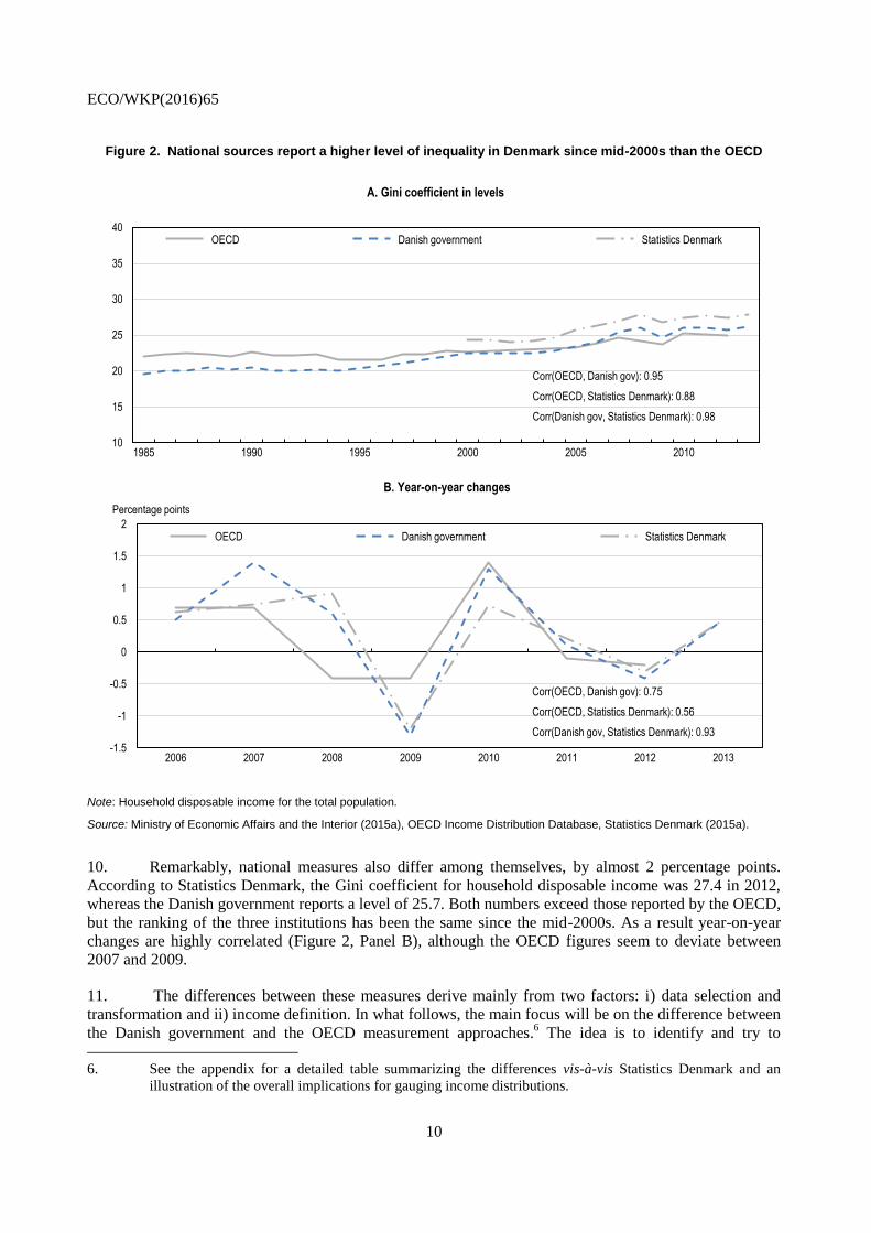
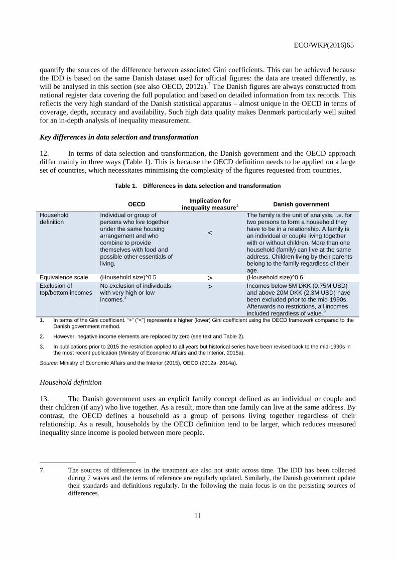


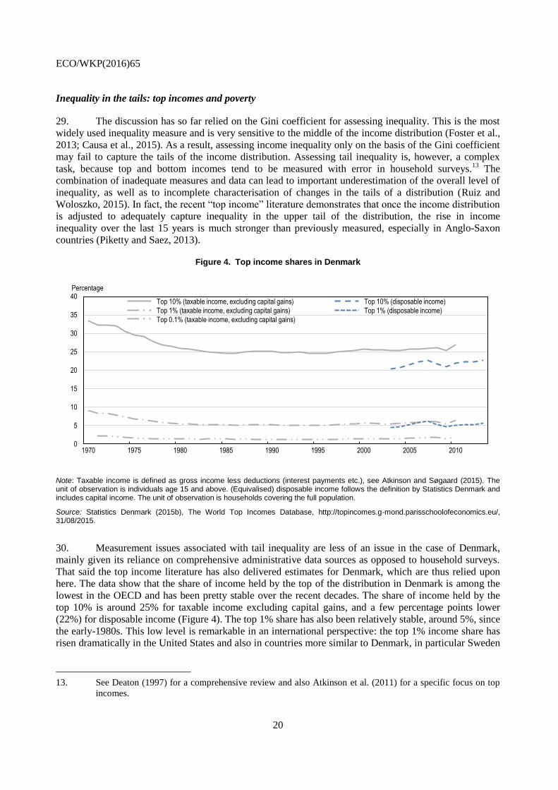

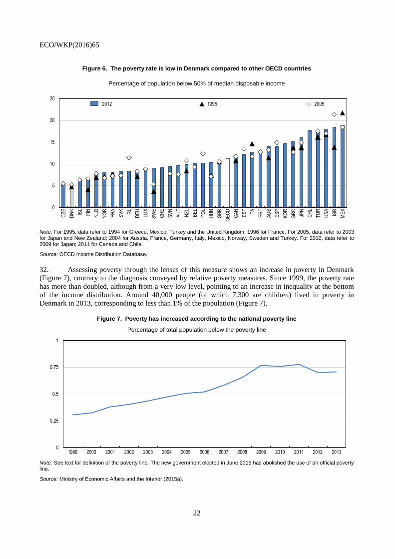


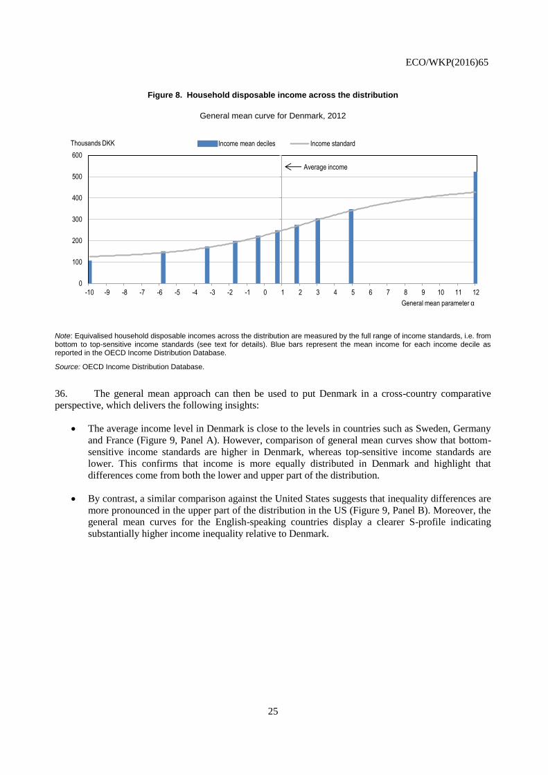


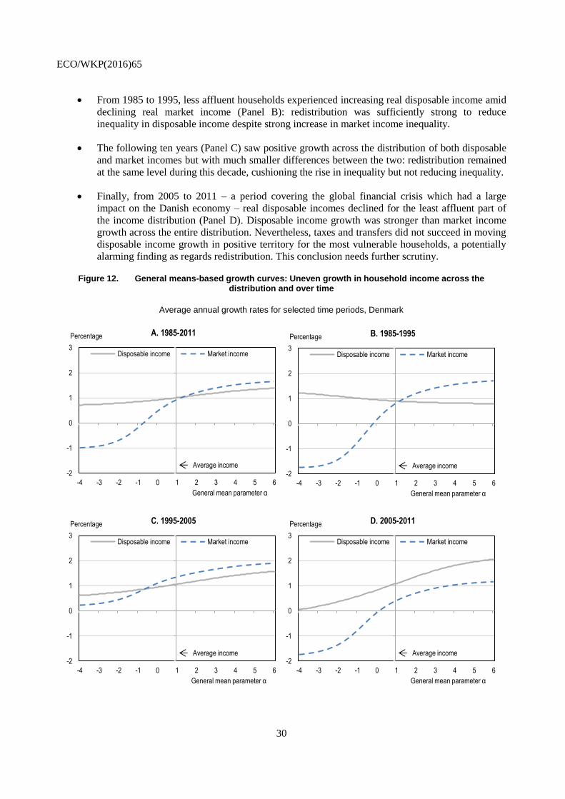


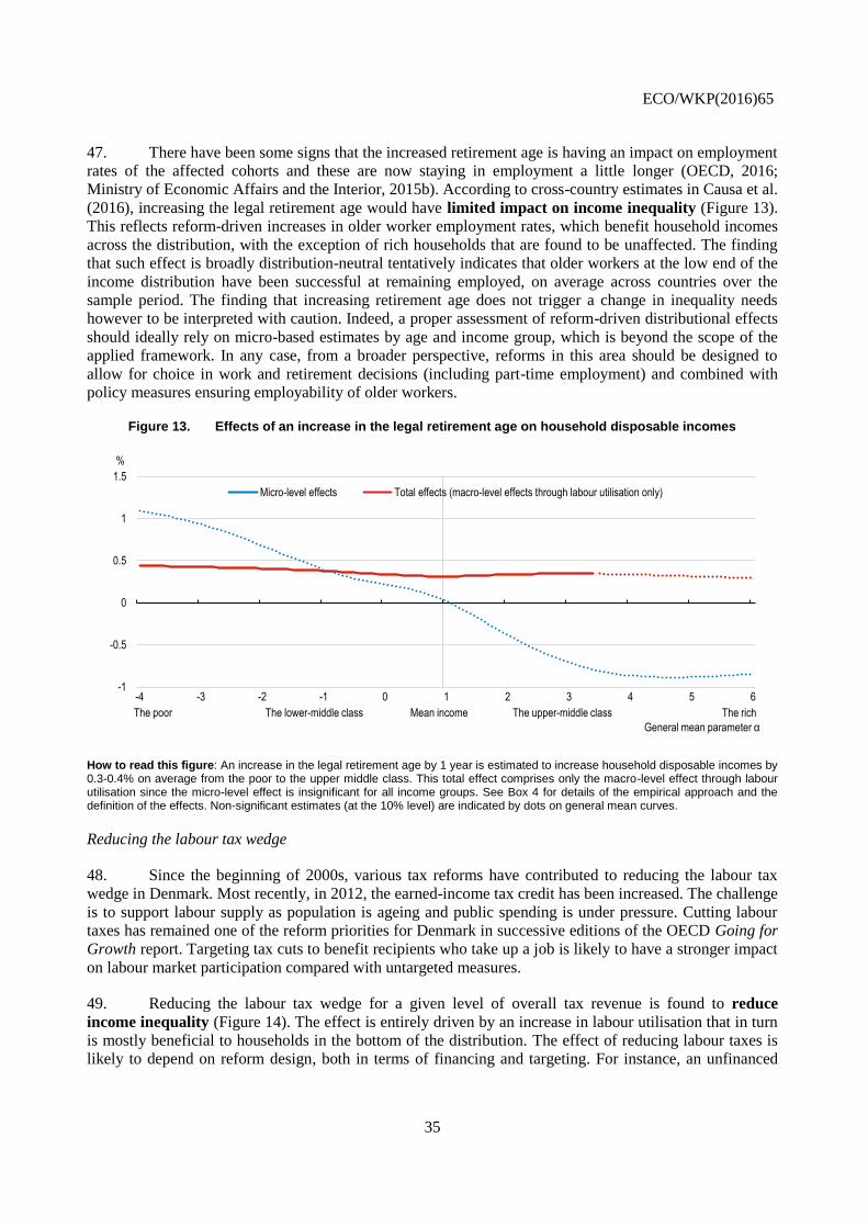


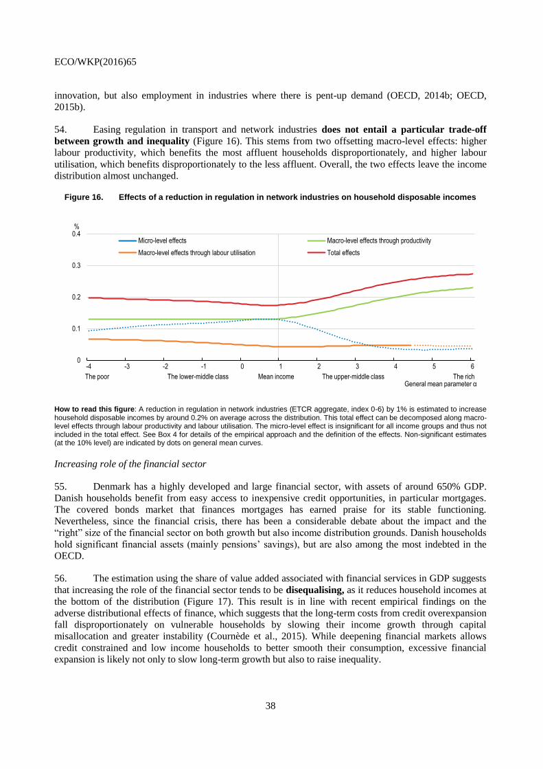


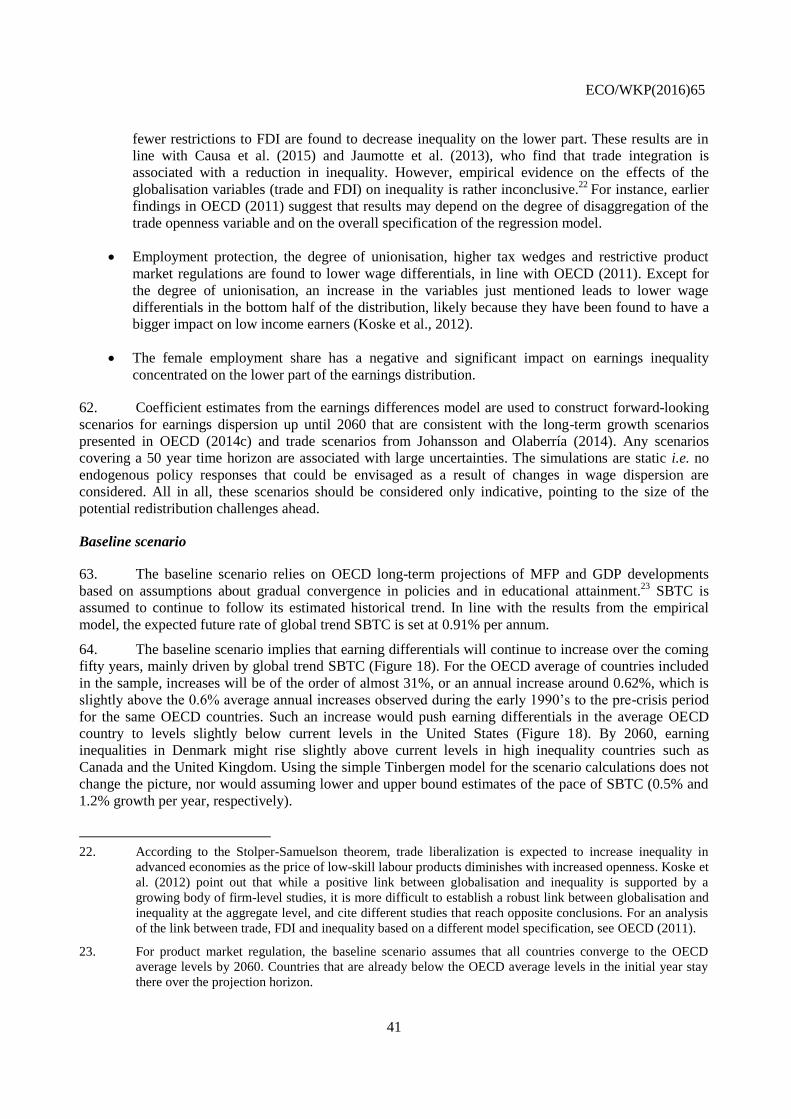


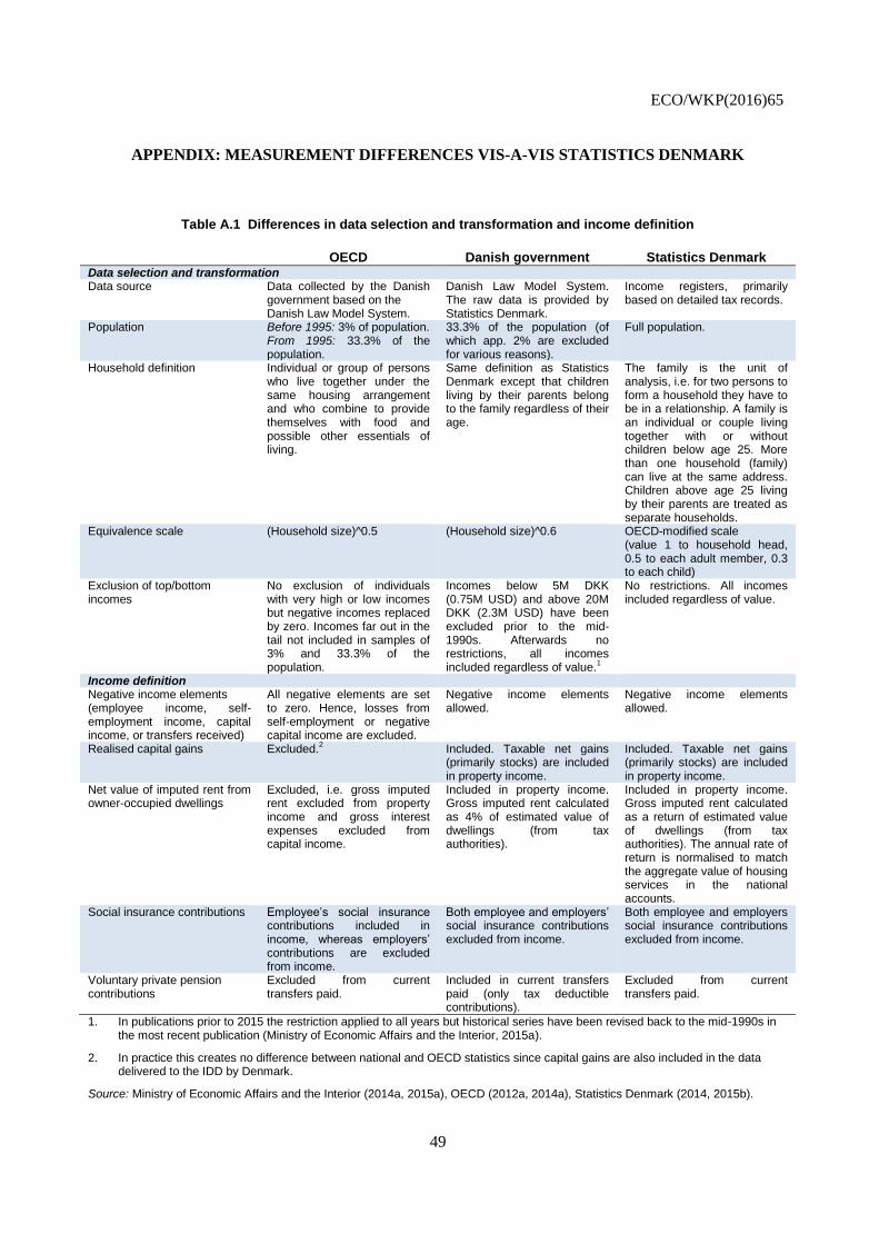


![Through the looking [Google] Glass](https://static.documents.pub/doc/80x56/58ed70341a28abdb228b46c9/through-the-looking-google-glass.jpg)

