1 Inertial Sensor Fusion for Limb Orientation Self-introduction: Hi my name is Mehdi Badrimanesh, I’m currently 26 years old, and I’m trying to get my Masters degree in mechatronic engineering at Khaje-nasir Toosy university (KNTU). I have written this tutorial for those of you who are interested in inertial sensor fusion for limb orientation. Thank you for putting away some time and reading it. Hope it’s useful (july/2019) Introduction In this tutorial, we discuss the topic of orientation estimation using inertial sensors fusion. We start by providing a brief background and motivation in 1.1 and explain what inertial sensors are and give a few concrete examples of relevant application areas of pose estimation using inertial sensors. In 1.2, we subsequently discuss how inertial sensors can be used to provide position and orientation information. Background and motivation The term inertial sensor is used to denote the combination of a threeaxis accelerometer and a three-axis gyroscope. Devices containing these sensors are commonly referred to as inertial measurement units (IMUs). Inertial sensors are nowadays also present in most modern smartphone, and in devices such as Wii controllers and virtual reality (VR) headsets,as shown in Figure 1.1. A gyroscope measures the sensor’s angular velocity, i.e. the rate of change of the sensor’s orientation. An accelerometer measures the external specific force acting on the sensor. The specific force consists of both the sensor’s acceleration and the earth’s gravity. Nowadays, many gyroscopes and accelerometers are based on microelectromechanical system (MEMS) technology. MEMS components are small, light, inexpensive, have low power consumption and short start-up times. Their accuracy has significantly increased over the years. Generally speaking, inertial sensors can be used to provide information about the pose of any object that they are rigidly attached to. It is also possible to combine multiple inertial sensors to obtain information about the pose of separate connected objects. Hence, inertial sensors can be used to track
Transcript
1
Inertial Sensor Fusion for Limb Orientation
Self-introduction: Hi my name is Mehdi Badrimanesh, I’m currently 26 years old, and I’m trying to get my Masters degree in mechatronic engineering at Khaje-nasir Toosy university (KNTU). I have written this tutorial for those of you who are interested in inertial sensor fusion for limb orientation. Thank you for putting away some time and reading it. Hope it’s useful (july/2019)
Introduction
In this tutorial, we discuss the topic of orientation estimation using inertial sensors fusion. We start by providing a brief background and motivation in 1.1 and explain what inertial sensors are and give a few concrete examples of relevant application areas of pose estimation using inertial sensors. In 1.2, we subsequently discuss how inertial sensors can be used to provide position and orientation
information.
Background and motivation
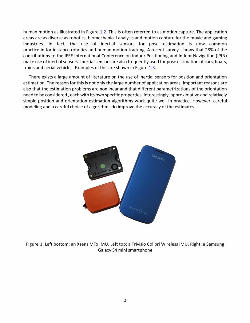
The term inertial sensor is used to denote the combination of a threeaxis accelerometer and a three-axis gyroscope. Devices containing these sensors are commonly referred to as inertial measurement units (IMUs). Inertial sensors are nowadays also present in most modern smartphone, and in devices such as Wii controllers and virtual reality (VR) headsets,as shown in Figure 1.1.
A gyroscope measures the sensor’s angular velocity, i.e. the rate of change of the sensor’s orientation. An accelerometer measures the external specific force acting on the sensor. The specific force consists of both the sensor’s acceleration and the earth’s gravity. Nowadays, many gyroscopes and accelerometers are based on microelectromechanical system (MEMS) technology. MEMS components are small, light, inexpensive, have low power consumption and short start-up times. Their accuracy has significantly increased over the years.
Generally speaking, inertial sensors can be used to provide information about the pose of any object that they are rigidly attached to. It is also possible to combine multiple inertial sensors to obtain information about the pose of separate connected objects. Hence, inertial sensors can be used to track
2
human motion as illustrated in Figure 1.2. This is often referred to as motion capture. The application areas are as diverse as robotics, biomechanical analysis and motion capture for the movie and gaming industries. In fact, the use of inertial sensors for pose estimation is now common practice in for instance robotics and human motion tracking. A recent survey shows that 28% of the contributions to the IEEE International Conference on Indoor Positioning and Indoor Navigation (IPIN) make use of inertial sensors. Inertial sensors are also frequently used for pose estimation of cars, boats, trains and aerial vehicles. Examples of this are shown in Figure 1.3.
There exists a large amount of literature on the use of inertial sensors for position and orientation estimation. The reason for this is not only the large number of application areas. Important reasons are also that the estimation problems are nonlinear and that different parametrizations of the orientation need to be considered , each with its own specific properties. Interestingly, approximative and relatively simple position and orientation estimation algorithms work quite well in practice. However, careful modeling and a careful choice of algorithms do improve the accuracy of the estimates.
Figure 1: Left bottom: an Xsens MTx IMU. Left top: a Trivisio Colibri Wireless IMU. Right: a Samsung Galaxy S4 mini smartphone
3
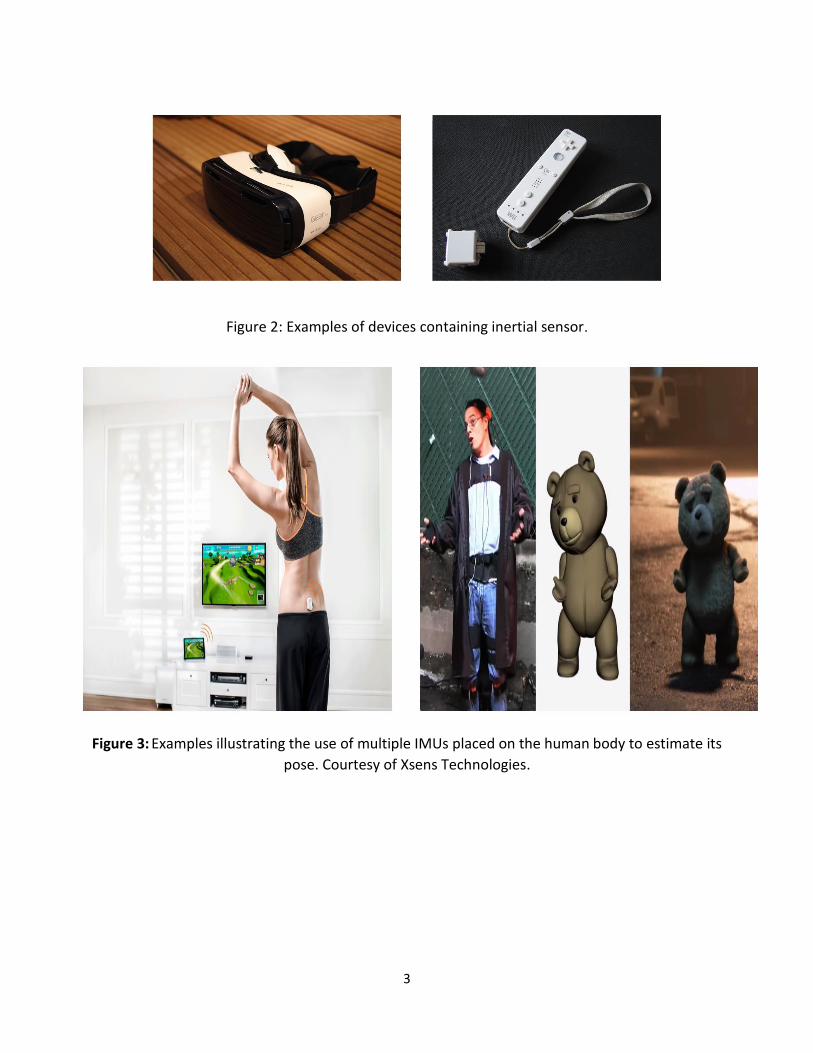
Figure 2: Examples of devices containing inertial sensor.
Figure 3: Examples illustrating the use of multiple IMUs placed on the human body to estimate its
pose. Courtesy of Xsens Technologies.
4
Figure 4: Examples illustrating the use of a single IMU placed on a moving object to estimate its pose.
Courtesy of Xsens Technologies
Figure 5: Schematic illustration of dead-reckoning, where the accelerometer measurements (external
specific force) and the gyroscope measurements (angular velocity) are integrated to position and
orientation.
Using inertial sensors for position and orientation estimation As illustrated in §1.1, inertial sensors are frequently used for navigation purposes where the position
and the orientation of a device are of interest. Integration of the gyroscope measurements provides information about the orientation of the sensor. After subtraction of the earth’s gravity, double integration of the accelerometer measurements provides information about the sensor’s position. To be able to subtract the earth’s gravity, the orientation of the sensor needs to be known. Hence, estimation of the sensor’s position and orientation are inherently linked when it comes to inertial sensors. The process of integrating the measurements from inertial sensors to obtain position and
5
orientation information, often called dead-reckoning, is summarized in Figure 1.4. If the initial pose would be known, and if perfect models for the inertial sensor measurements would exist, the process illustrated in Figure 1.4 would lead to perfect pose estimates. In practice, however, the inertial measurements are noisy and biased as will be discussed in more detail in §2.4. Because of this, the integration steps from angular velocity to rotation and from acceleration to position introduce integration drift. This is illustrated in Example 1.1.
Using inertial sensors for position and orientation estimation
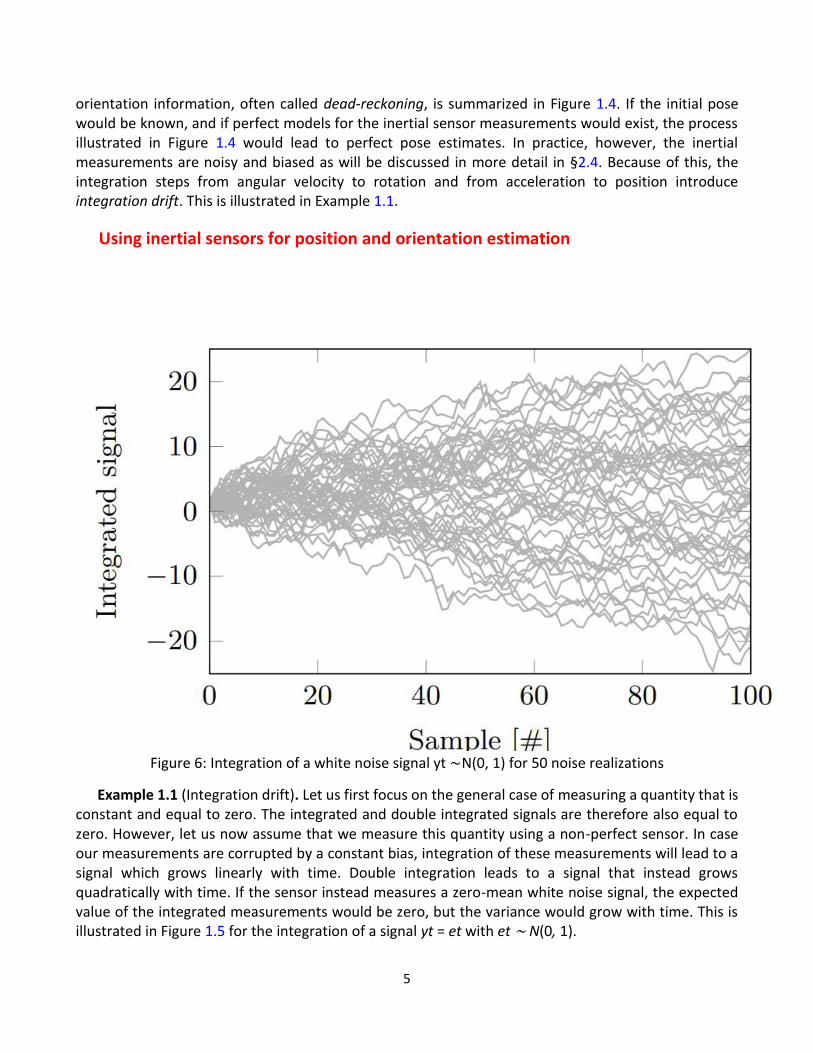
Figure 6: Integration of a white noise signal yt ∼ N(0, 1) for 50 noise realizations
Example 1.1 (Integration drift). Let us first focus on the general case of measuring a quantity that is constant and equal to zero. The integrated and double integrated signals are therefore also equal to zero. However, let us now assume that we measure this quantity using a non-perfect sensor. In case our measurements are corrupted by a constant bias, integration of these measurements will lead to a signal which grows linearly with time. Double integration leads to a signal that instead grows quadratically with time. If the sensor instead measures a zero-mean white noise signal, the expected value of the integrated measurements would be zero, but the variance would grow with time. This is illustrated in Figure 1.5 for the integration of a signal yt = et with et ∼ N(0, 1).
6
Hence, integration drift is both due to integration of a constant bias and due to integration of noise.
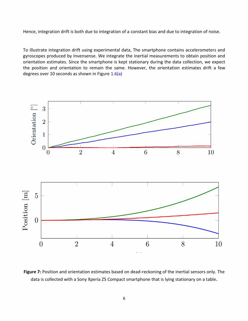
To illustrate integration drift using experimental data, The smartphone contains accelerometers and gyroscopes produced by Invensense. We integrate the inertial measurements to obtain position and orientation estimates. Since the smartphone is kept stationary during the data collection, we expect the position and orientation to remain the same. However, the orientation estimates drift a few degrees over 10 seconds as shown in Figure 1.6(a)
Figure 7: Position and orientation estimates based on dead-reckoning of the inertial sensors only. The
data is collected with a Sony Xperia Z5 Compact smartphone that is lying stationary on a table.
7
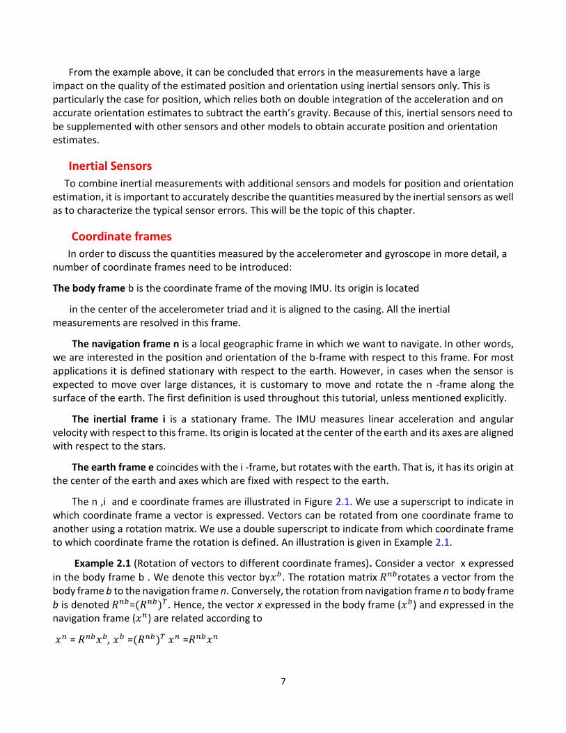
From the example above, it can be concluded that errors in the measurements have a large impact on the quality of the estimated position and orientation using inertial sensors only. This is particularly the case for position, which relies both on double integration of the acceleration and on accurate orientation estimates to subtract the earth’s gravity. Because of this, inertial sensors need to be supplemented with other sensors and other models to obtain accurate position and orientation estimates.
Inertial Sensors
To combine inertial measurements with additional sensors and models for position and orientation estimation, it is important to accurately describe the quantities measured by the inertial sensors as well as to characterize the typical sensor errors. This will be the topic of this chapter.
Coordinate frames In order to discuss the quantities measured by the accelerometer and gyroscope in more detail, a
number of coordinate frames need to be introduced:
The body frame b is the coordinate frame of the moving IMU. Its origin is located
in the center of the accelerometer triad and it is aligned to the casing. All the inertial measurements are resolved in this frame.
The navigation frame n is a local geographic frame in which we want to navigate. In other words, we are interested in the position and orientation of the b-frame with respect to this frame. For most applications it is defined stationary with respect to the earth. However, in cases when the sensor is expected to move over large distances, it is customary to move and rotate the n -frame along the surface of the earth. The first definition is used throughout this tutorial, unless mentioned explicitly.
The inertial frame i is a stationary frame. The IMU measures linear acceleration and angular velocity with respect to this frame. Its origin is located at the center of the earth and its axes are aligned with respect to the stars.
The earth frame e coincides with the i -frame, but rotates with the earth. That is, it has its origin at the center of the earth and axes which are fixed with respect to the earth.
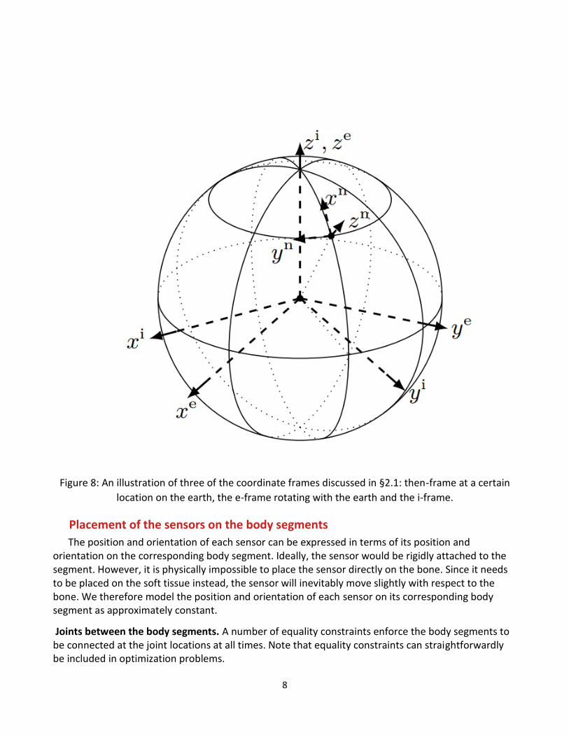
The n ,i and e coordinate frames are illustrated in Figure 2.1. We use a superscript to indicate in which coordinate frame a vector is expressed. Vectors can be rotated from one coordinate frame to another using a rotation matrix. We use a double superscript to indicate from which coordinate frame to which coordinate frame the rotation is defined. An illustration is given in Example 2.1.
Example 2.1 (Rotation of vectors to different coordinate frames). Consider a vector x expressed in the body frame b . We denote this vector by𝑥𝑏. The rotation matrix 𝑅𝑛𝑏rotates a vector from the body frame b to the navigation frame n. Conversely, the rotation from navigation frame n to body frame b is denoted 𝑅𝑛𝑏=(𝑅𝑛𝑏)𝑇. Hence, the vector x expressed in the body frame (𝑥𝑏) and expressed in the navigation frame (𝑥𝑛) are related according to
𝑥𝑛 = 𝑅𝑛𝑏𝑥𝑏, 𝑥𝑏 =(𝑅𝑛𝑏)𝑇 𝑥𝑛 =𝑅𝑛𝑏𝑥𝑛
8
Figure 8: An illustration of three of the coordinate frames discussed in §2.1: then-frame at a certain
location on the earth, the e-frame rotating with the earth and the i-frame.
Placement of the sensors on the body segments
The position and orientation of each sensor can be expressed in terms of its position and orientation on the corresponding body segment. Ideally, the sensor would be rigidly attached to the segment. However, it is physically impossible to place the sensor directly on the bone. Since it needs to be placed on the soft tissue instead, the sensor will inevitably move slightly with respect to the bone. We therefore model the position and orientation of each sensor on its corresponding body segment as approximately constant.
Joints between the body segments. A number of equality constraints enforce the body segments to be connected at the joint locations at all times. Note that equality constraints can straightforwardly be included in optimization problems.
9
Exclusion of magnetometer measurements .The magnetic field in indoor environments is not constant, This is specifically of concern in motion capture applications, since the magnetic field measured at the different sensor locations is typically different. Because of this, we do not include. magnetometer measurements in the model. The inclusion of the equality constraints enforcing the body segments to be connected allows us to do so, since incorporating these constraints, the sensor’s relative position and orientation become observable as long as the subject is not standing completely still. As before, we denote the time-varying states by 𝑥𝑡and the constant parameters by 𝜃. However, to highlight the different parts of the model ,we split the states 𝑥𝑡 in states 𝑥𝑡
𝑠𝑖pertaining to the sensor 𝑠𝑖and states 𝑥𝑡
𝐵𝑖pertaining to the body segment 𝐵𝑖, for i = 1, . . . ,𝑁𝑠. Here, 𝑁𝑠 is the number of sensors attached to the body and it is assumed to be equal to the number of body segments that are modeled. Using this notation, the optimization problem that is solved in can be summarized as
𝑚𝑖𝑛 −∑ ∑log𝑝(𝑥𝑡𝑠𝑖|𝑥𝑡−1
𝑠𝑖) −
𝑁𝑠
𝑖=1
𝑁𝑡
𝑡=2⏟ Dynamics of the state 𝑥𝑡
𝑠𝑖
∑ ∑log𝑝(𝑥𝑡𝐵𝑖|𝑥𝑡
𝑠𝑖)
𝑁𝑠
𝑖=1
𝑁𝑡
𝑡=1⏟ Placement of sensor S𝑖 on body segment B𝑖
−∑log 𝑝(𝑥1𝑠𝑖)
𝑁𝑠
𝑖=1
−∑log 𝑝(𝜃𝑠𝑖)
𝑁𝑠
𝑖=1⏟ pior
c(x1:N) = 0 where the number of time steps is denoted NT and c(x1:N) denote the equality constraints from assuming that the body segments are connected at the joints.
Concluding Remarks
The goal of this tutorial was not to give a complete overview of all algorithms that can be used for position and orientation estimation. Instead, our aim was to give a pedagogical introduction to the topic of position and orientation estimation using inertial sensors, allowing newcomers to this problem to get up to speed as fast as possible by reading one paper. By integrating the inertial sensor measurements (so-called dead-reckoning), it is possible to obtain information about the position and orientation of the sensor. However, errors in the measurements will accumulate and the estimates will drift. Because of this , to obtain accurate position and orientation estimates using inertial measurements, it is necessary to use additional sensors and additional models. In this tutorial, we have considered two separate estimation problems. The first is orientation estimation using inertial and magnetometer measurements, assuming that the acceleration of the sensor is approximately zero. Including magnetometer measurements removes the drift in the heading direction, while assuming that the acceleration is approximately zero removes the drift in the inclination. The second estimation problem that we have considered is pose estimation using inertial and position measurements. Using inertial measurements, the position and orientation estimates are coupled and the position measurements therefore provide information also about the orientation.


![[Phys 6006][Ben Williams][Inertial Confinement Fusion]](https://static.documents.pub/doc/80x56/58a7db721a28ab8a7e8b61cb/phys-6006ben-williamsinertial-confinement-fusion.jpg)


