Inference in non parametric Hidden Markov Models

Inference in non parametric Hidden MarkovModels

Elisabeth Gassiat

Universite Paris-Sud (Orsay) and CNRS

Van Dantzig Seminar, June 2017

E.Gassiat (UPS and CNRS) Nonparametric HMM Leiden 2017 1 / 47

Hidden Markov models (HMMs)

Zk Zk+1

Xk Xk+1

Observations (Xk)k≥1 are independent conditionnally to (Zk)k≥1

L ((Xk)k≥1|(Zk)k≥1) =⊗k≥1

L (Xk |Zk)

Latent (unobserved) variables (Zk)k≥1 form a Markov chain


Finite state space stationary HMMs

The Markov chain is stationary, has finite state space {1, . . . ,K}and transition matrix Q. The stationary distribution is denoted µ.

Conditionnally to Zk = j , Xk has emission distribution Fj .

The marginal distribution of any Xk is

K∑j=1

µ (j)Fj

A finite state space HMM is a finite mixture with Markov regime


Finite state space stationary HMMs

The Markov chain is stationary, has finite state space {1, . . . ,K}and transition matrix Q. The stationary distribution is denoted µ.

Conditionnally to Zk = j , Xk has emission distribution Fj .

The marginal distribution of any Xk is

K∑j=1

µ (j)Fj

A finite state space HMM is a finite mixture with Markov regime


The use of hidden Markov models

Modeling dependent data arising from heterogeneous populations.

Markov regime : leads to efficient algorithms to compute :

Filtering/prediction/smoothing/ probabilities(Forward/Backward recursions) : given a set of observations,the probability of hidden states.

Maximum a posteriori (prediction of hidden states) ; Viterbi’salgorithm.

Likelihoods and EM algorithms : estimation of the transitionmatrix Q and the emission distributions F1, . . . , FK

MCMC Bayesian methods


The use of hidden Markov models

Modeling dependent data arising from heterogeneous populations.

Markov regime : leads to efficient algorithms to compute :

Filtering/prediction/smoothing/ probabilities(Forward/Backward recursions) : given a set of observations,the probability of hidden states.

Maximum a posteriori (prediction of hidden states) ; Viterbi’salgorithm.

Likelihoods and EM algorithms : estimation of the transitionmatrix Q and the emission distributions F1, . . . , FK

MCMC Bayesian methods


The parametric/non parametric story

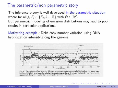
The inference theory is well developed in the parametric situationwhere for all j , Fj ∈ {Fθ, θ ∈ Θ} with Θ ⊂ Rd .But parametric modeling of emission distributions may lead to poorresults in particular applications.

Motivating example : DNA copy number variation using DNAhybridization intensity along the genome


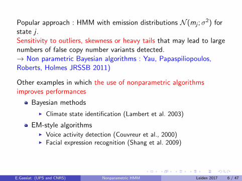
Popular approach : HMM with emission distributions N (mj ;σ2) for

state j .Sensitivity to outliers, skewness or heavy tails that may lead to largenumbers of false copy number variants detected.→ Non parametric Bayesian algorithms : Yau, Papaspiliopoulos,Roberts, Holmes JRSSB 2011)

Other examples in which the use of nonparametric algorithmsimproves performances

Bayesian methods

I Climate state identification (Lambert et al. 2003)

EM-style algorithmsI Voice activity detection (Couvreur et al., 2000)I Facial expression recognition (Shang et al. 2009)


Finite state space non parametric HMMs

The marginal distribution of any Xk is∑K

j=1 µ (j)Fj

Non parametric mixtures are not identifiable with no furtherassumptions

µ (1)F1 + µ (2)F2 + . . .+ µ (K )FK

= (µ(1)+µ(2))

[µ (1)

µ(1) + µ(2)F1 +

µ (2)

µ(1) + µ(2)F2

]+ . . .+µ (K )FK

=µ (1)

2F1 +

[µ(1)

2 F1 + µ (2)F2

]µ(1)

2 + µ (2)+ . . .+ µ (K )FK

Why do non parametric HMM algorithms work ? ? ? ?

Dependence of observed variables has to help !


Basic questions

Denote F = (F1, . . . ,FK ).

For m an integer, let P(m)K ;Q;F be the distribution of (X1, . . . ,Xm).

The sequence of observed variables has mixing properties : adaptive

estimation of P(m)K ;Q;F is possible. Can one get information on K , Q

and F from an estimator P(m) of P(m)K ;Q;F ?

Identifiability : for some m,

P(m)K1;Q1;F1

= P(m)K2;Q2;F2

=⇒ K1 = K2, Q1 = Q2, F1 = F2.

Inverse problem : Build estimators K , Q and F such that one

may deduce consistency/rates from those of P(m) as an

estimator of P(m)K ;Q;F.


Joint work with Judith Rousseau (translated emission distributions ;Bernoulli 2016)

Joint work with Alice Cleynen and Stephane Robin (Generalidentifiability ; Stat. and Comp. 2016),Yohann De Castro and Claire Lacour (Adaptive estimation via modelselection and least squares ; JMLR 2016),Yohann De Castro and Sylvain Le Corff (Spectral estimation andestimation of filtering/smoothing probabilities ; IEEE IT to appear),

Work by Elodie Vernet (Bayesian estimation ; consistency EJS 2015and rates Bernoulli in revision)

Work by Luc Lehericy (Estimation of K ; submitted ; state by stateadaptivity ; submitted)

Work by Augustin Touron (Climate applications ; PHD in progress)


Identifiability/inference theoretical results innonparametric HMMs

1 Identifiability in non parametric finite translation HMMs andextensions

2 Identifiability in non parametric general HMMs

3 Generic methods

4 Inverse problem inequalities

5 Further works





3 Generic methods


5 Further works


Translated emission distributions

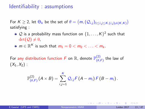
Here we assume that there exists a distribution function F and realnumbers m1, . . . ,mK such that

Fj (·) = F (· −mj) , j = 1, . . . ,K .

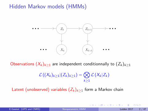
The observations follow

Xt = mZt + εt , t ≥ 1,

where the variables εt , t ≥ 1, are i.i.d. with distribution function F ,and are independent of the Markov chain (Zt)t≥1.

Previous work : independent variables ; K ≤ 3 ; symmetryassumption on F : Bordes, Mottelet, Vandekerkhove (Annals of Stat.2006) ; Hunter, Wang, Hettmansperger (Annals of Stat. 2007) ;Butucea, Vandekerkhove (Scandinavian J. of Stat, to appear).


Identifiability : assumptions

For K ≥ 2, let Θk be the set of θ =(m, (Qi ,j)1≤i ,j≤K ,(i ,j)6=(K ,K)

)satisfying :

Q is a probability mass function on {1, . . . ,K}2 such thatdet(Q) 6= 0,

m ∈ RK is such that m1 = 0 < m2 < . . . < mk .

For any distribution function F on R, denote P(2)(θ,F ) the law of

(X1,X2) :

P(2)(θ,F ) (A× B) =

K∑i ,j=1

Qi ,jF (A−mi )F (B −mi ) .


Identifiability result

Theorem [ EG, J. Rousseau (Bernoulli 2016)]

Let F and F be distribution function on R, θ ∈ ΘK and θ in ΘK .Then

P(2)θ,F = P(2)

θ,F=⇒ K = K , θ = θ and F = F.

No assumption on F !

HMM not needed ; dependent (stationary) state variablessuffice.

Extension (by projections) to multidimensional variables.

Identification of `-marginal distribution, i.e. the law of(Z1, . . . ,Z`), K and F using the law of (X1, . . . ,X`).


Identifiability : sketch of proofφF : characteristic function of F ; φF : c.f. of F ;φθ,i : (φθ,i ) c.f. of the law of mZi

under Pθ,F , (under Pθ,F ) ;Φθ : (Φθ) c.f. of the law of (mZ1 ,mZ2) under Pθ,F (under Pθ,F ).

The c.f. of the law of X1, of X2, then of (X1,X2), give

φF (t)φθ,1 (t) = φF (t)φθ,1 (t) ,

φF (t)φθ,2 (t) = φF (t)φθ,2 (t) ,

φF (t1)φF (t2) Φθ (t1, t2) = φF (t1)φF (t2) Φθ (t1, t2) .

We thus get for all (t1, t2) ∈ R2,

φF (t1)φF (t2) Φθ (t1, t2)φθ,1 (t1)φθ,2 (t2)

= φF (t1)φF (t2) Φθ (t1, t2)φθ,1 (t1)φθ,2 (t2) .


Identifiability : sketch of proof

Thus on a neighborhood of 0 in which φF is non zero :

Φθ (t1, t2)φθ,1 (t1)φθ,2 (t2) = Φθ (t1, t2)φθ,1 (t1)φθ,2 (t2) .

Then

Equation extended to the complex plane (entire functions).

The set of zeros of φθ,1 coincides with the set of zeros of φθ,1(here det(Q) 6= 0 is used).

Hadamard’s factorization theorem allows to prove thatφθ,1 = φθ,1.

Same proof for φθ,2 = φθ,2, leading to Φθ = Φθ, and thenφF = φF

Finally the characteristic function characterizes the law, so thatK = K , θ = θ and F = F .


Identifiability : estimation of θ

Φθ (t1, t2)φX1 (t1)φX2 (t2)− Φ(X1,X2) (t1, t2)φθ,1 (t1)φθ,2 (t2) = 0.

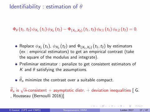
Replace φX1 (t1), φX2 (t2) and Φ(X1,X2) (t1, t2) by estimators(ex : empirical estimators) to get an empirical contrast (takethe square of the modulus and integrate).

Preliminar estimator : penalize to get consistent estimators ofK and θ satisfying the assumptions.

θn minimize the contrast over a suitable compact.

θn is√n-consistent + asymptotic distr. + deviation inequalities [ G.

, Rousseau (Bernoulli 2016)]





3 Generic methods


5 Further works


Finite state space HMM : Connexion with mixtures ofindependent variablesThe distribution of (X1,X2,X3) may be written as

P(3)Q,F =

K∑i=1

K∑j=1

K∑m=1

µ (i)Qi ,jQj ,mFi ⊗ Fj ⊗ Fm

=K∑j=1

µ (j)

(K∑i=1

µ (i)Qi ,j

µ (j)Fi

)⊗ Fj ⊗

(K∑

m=1

Qj ,mFm

)

=K∑j=1

µ (j)Gj ,1 ⊗ Gj ,2 ⊗ Gj ,3

which is a mixture of K populations, in each population theobservation is that of independent variables.

Z1 and Z3 are independent conditionally to Z2.

→ Use results about mixtures of independent variables.


An old result by Kruskal

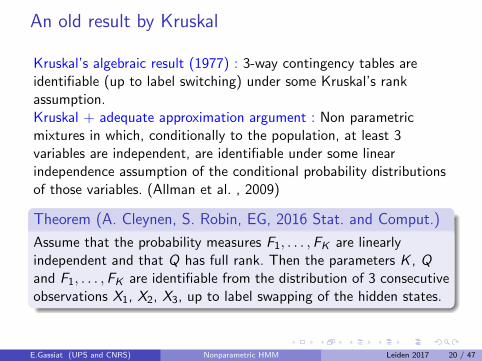
Kruskal’s algebraic result (1977) : 3-way contingency tables areidentifiable (up to label switching) under some Kruskal’s rankassumption.Kruskal + adequate approximation argument : Non parametricmixtures in which, conditionally to the population, at least 3variables are independent, are identifiable under some linearindependence assumption of the conditional probability distributionsof those variables. (Allman et al. , 2009)

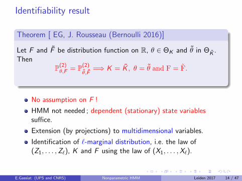
Theorem (A. Cleynen, S. Robin, EG, 2016 Stat. and Comput.)

Assume that the probability measures F1, . . . ,FK are linearlyindependent and that Q has full rank. Then the parameters K , Qand F1, . . . ,FK are identifiable from the distribution of 3 consecutiveobservations X1, X2, X3, up to label swapping of the hidden states.


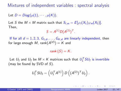
Mixtures of independent variables : spectral analysisWorks by Anandkumar, Dai, Hsu, Kakade, Song, Zhang, Xie.

Let X = (X1;X2;X3) have distribution ⊗3d=1Gj ,d conditionally to

Z = j so that X has distribution

K∑j=1

µ (j)⊗3d=1 Gj ,d

Let ϕ1, . . . , ϕM be M real valued functions.For d = 1, 2, 3, define A(d) the M × K matrix such that

A(d)l ,j =

∫ϕldGj ,d = E [ϕl(Xd)|Z = j ]

A(d) =

∫ϕ1dG1,d · · ·

∫ϕ1dGK ,d

......

...∫ϕMdG1,d · · ·

∫ϕMdGK ,d


Mixtures of independent variables : spectral analysis

Let D = Diag(µ(1), · · · , µ(K )).

Let S the M ×M matrix such that Sl ,m = E [ϕl(X1)ϕm(X2)].Then,

S = A(1)D(A(2))T .

If for all d = 1, 2, 3, G1,d , . . . ,GK ,d are linearly independent, thenfor large enough M, rank(A(d)) = K and

rank (S) = K .

Let U1 and U2 be M × K matrices such that UT1 SU2 is invertible

(may be found by SVD of S).

UT1 SU2 =

(UT

1 A(1))D(

(A(2))TU2

).


Mixtures of independent variables : spectral analysisDefine T be the M ×M ×M tensor such that

T (l1, l2, l3) = E [ϕl1(X1)ϕl2(X2)φl3(X3)].

Let V ∈ RM , and define T [V ] the M ×M matrix such that

T [V ]l ,m = E [ϕl(X1)ϕm(X2)〈V ,Φ(X3)〉]

where Φ(X3) = (ϕh(X3))1≤h≤M . Then

T [V ] = A(1)D · Diag(

(A(3))TV)

(A(2))T

DefineB(V ) = (UT

1 T [V ]U2)(UT1 SU2)−1.

Then, one has

B(V ) = (UT1 A(1))Diag

((A(3))TV

)(UT

1 A(1))−1.



UT1 SU2 =

(UT

1 A(1))D(

(A(2))TU2

)(UT

1 SU2

)−1=(

(A(2))TU2

)−1D−1

(UT

1 A(1))−1

T [V ] = A(1)D · Diag(

(A(3))TV)

(A(2))T

B(V ) = (UT1 T [V ]U2)(UT

1 SU2)−1

= UT1 A(1)D · Diag

((A(3))TV

)(A(2))TU2(UT

1 SU2)−1

= UT1 A(1)Diag

((A(3))TV

)· D(A(2))TU2(UT

1 SU2)−1

= (UT1 A(1))Diag

((A(3))TV

)(UT

1 A(1))−1.



Recall

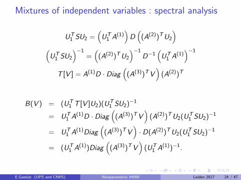
B(V ) = (UT1 T [V ]U2)(UT

1 SU2)−1 = (UT1 A(1))Diag

((A(3))TV

)(UT

1 A(1))−1.

All matrices B(V ) have the same eigenvectors, and eigenvalues thecoordinates of (A(3))TV .By exploring various vectors V , one may recover A(3). Theeigenvectors stay the same when permuting coordinates 2 and 3 ofthe observed variable, so that one may recover A(2), and thus alsoA(1). Recovering D is then also possible. Then, by taking M toinfinity, one may recover the whole distributions G1,j , G2,j and G3,j ,j = 1, . . . ,K .

One may recover µ(1), . . . , µ(K ) and G1,j , G2,j and G3,j ,j = 1, . . . ,K using Singular Value/ Eigen Value decompositions ofmatrices built from the distribution of X = (X1,X2,X3).


Spectral analysis : estimation

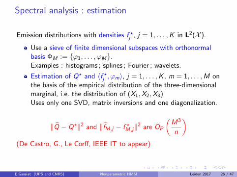
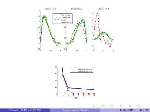
Emission distributions with densities f ?j , j = 1, . . . ,K in L2(X ).

Use a sieve of finite dimensional subspaces with orthonormalbasis ΦM := {ϕ1, . . . , ϕM}.Examples : histograms ; splines ; Fourier ; wavelets.

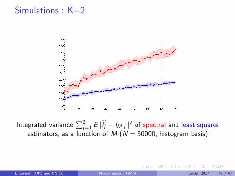
Estimation of Q? and 〈f ?j , ϕm〉, j = 1, . . . ,K , m = 1, . . . ,M onthe basis of the empirical distribution of the three-dimensionalmarginal, i.e. the distribution of (X1,X2,X3)Uses only one SVD, matrix inversions and one diagonalization.

‖Q − Q?‖2 and ‖fM,j − f ?M,j‖2 are OP

(M3

n

)(De Castro, G., Le Corff, IEEE IT to appear)





3 Generic methods


5 Further works


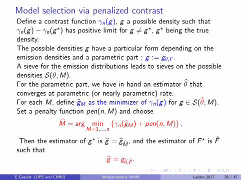
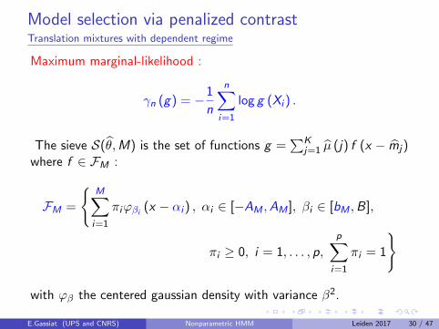
Model selection via penalized contrastDefine a contrast function γn(g), g a possible density such thatγn(g)− γn(g?) has positive limit for g 6= g?, g? being the truedensity.The possible densities g have a particular form depending on theemission densities and a parametric part : g := gθ,F .A sieve for the emission distributions leads to sieves on the possibledensities S(θ,M).For the parametric part, we have in hand an estimator θ thatconverges at parametric (or nearly parametric) rate.For each M, define gM as the minimizer of γn(g) for g ∈ S(θ,M).Set a penalty function pen(n,M) and choose

M = arg minM=1,...,n

{γn(gM) + pen(n,M)} .

Then the estimator of g? is g = gM

, and the estimator of F ? is Fsuch that

g = gθ,F.


Model selection via penalized contrastTranslation mixtures with dependent regime

Recall that the observations follow :

Xt = mZt + εt , t ≥ 1,

where the variables εt , t ≥ 1, are i.i.d. with distribution function F ,and are independent of the Markov chain (Zt)t≥1.When θ = ((mj)j , (Qi ,j)i ,j) is known, one may recover F from themarginal density gθ,F of Xt .If F has density f , then gθ,f := gθ,F is given by :

gθ,f (x) =K∑j=1

µ (j) f (x −mj) .

where µ(i) =∑K

j=1 Qi ,j . Given the estimator

θn = ((mi )1≤i≤k? , (Qi ,j)(i ,j)6=(k?,k?)), denote µ(i) =∑k?

j=1 Qi ,j .


Model selection via penalized contrastTranslation mixtures with dependent regime

Maximum marginal-likelihood :

γn (g) = −1

n

n∑i=1

log g (Xi ) .

The sieve S(θ,M) is the set of functions g =∑K

j=1 µ (j) f (x − mj)where f ∈ FM :

FM =

{M∑i=1

πiϕβi (x − αi ) , αi ∈ [−AM ,AM ], βi ∈ [bM ,B],

πi ≥ 0, i = 1, . . . , p,

p∑i=1

πi = 1

}

with ϕβ the centered gaussian density with variance β2.


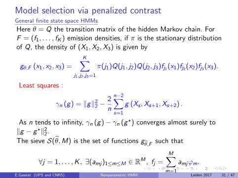
Model selection via penalized contrastGeneral finite state space HMMs

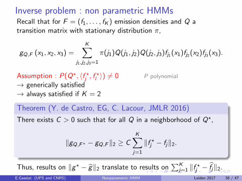
Here θ = Q the transition matrix of the hidden Markov chain. ForF = (f1, . . . , fK ) emission densities, if π is the stationary distributionof Q, the density of (X1,X2,X3) is given by

gθ,F (x1, x2, x3) =K∑

j1,j2,j3=1

π(j1)Q(j1, j2)Q(j2, j3)fj1(x1)fj2(x2)fj3(x3).

Least squares :

γn (g) = ‖g‖22 −

2

n

n−2∑s=1

g (Xs ,Xs+1,Xs+2) .

As n tends to infinity, γn (g)− γn (g?) converges almost surely to‖g − g?‖2

2.

The sieve S(θ,M) is the set of functions gθ,F

such that

∀j = 1, . . . ,K , ∃(amj)1≤m≤M ∈ RM , fj =M∑

m=1

amjϕm.


Oracle inequalities (in general)

There exist constants κ, C and n0 such that : if

pen(n,M) ≥ κ complexity(M)log n

n,

then for all x > 0, for all n ≥ n0, with probability 1− e−x , it holds

D2(g , g?) ≤ C { infM

[d2(g?M , g

?) + pen(n,M)]

+ small terms } .

Proof : concentration inequality + control of the complexity ofthe Sieve (ex : using bracketing entropy).

Adaptive rates ; automatic best compromise bias/variance.

Penalty in practice : slope heuristics.


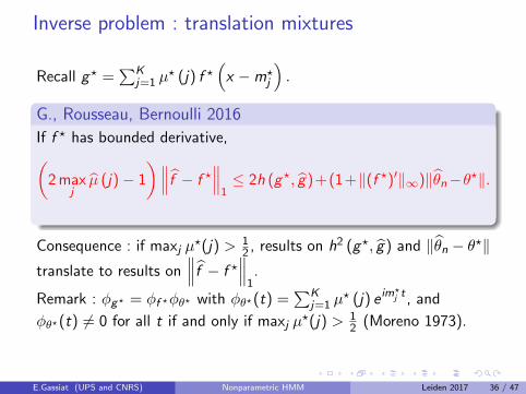
Oracle inequalities : Translation mixtures and HMMs

Additional difficulty : deal with θ in γn.C depends here on the hidden chain (concentration inequality fordependent variables).

Translation mixtures with dependent regimeOracle inequality using penalized m.l.e (G. , Rousseau [Bernoulli2016]).D2(g , g?) : Hellinger’s distance.d2(g?M , g

?) : Kullback’s divergence.

General finite state space HMMsOracle inequality using least squares (De Castro, G. Lacour [JMLR2016]).D2(g , g?) and d2(g?M , g

?) : L2-square distance.





3 Generic methods


5 Further works


General question

Consistent estimation of g? translates to consistent estimation ofF ?.

Do adaptive minimax rates for the estimation of g? translate toadaptive minimax rates for the estimation of F ? ?


Inverse problem : translation mixtures

Recall g? =∑K

j=1 µ? (j) f ?

(x −m?

j

).

G., Rousseau, Bernoulli 2016

If f ? has bounded derivative,(2 max

jµ (j)− 1

)∥∥∥f − f ?∥∥∥

1≤ 2h (g?, g)+(1+‖(f ?)′‖∞)‖θn−θ?‖.

Consequence : if maxj µ?(j) > 1

2 , results on h2 (g?, g) and ‖θn − θ?‖translate to results on

∥∥∥f − f ?∥∥∥

1.

Remark : φg? = φf ?φθ? with φθ?(t) =∑K

j=1 µ? (j) e im

?j t , and

φθ?(t) 6= 0 for all t if and only if maxj µ?(j) > 1

2 (Moreno 1973).


ProofProof : starts from ‖g? − g‖2

1 ≤ 4h2 (g?, g) . Then,

‖g? − g‖1 = ‖K∑j=1

µ? (j) f ?(y −m?

j

)−

K∑j=1

µ (j) f (· − mj) ‖1

≥ ‖K∑j=1

µ (j) (f − f ?) (· − mj) ‖1

−‖K∑j=1

µ? (j) f ?(y −m?

j

)−

K∑j=1

µ (j) f ? (· − mj) ‖1

≥ ‖K∑j=1

µ (j) (f − f ?) (· − mj) ‖1 − (1 + ‖(f ?)′‖∞)‖θn − θ?‖.

Then using the triangle inequality,

‖K∑j=1

µ (j) (f − f ?) (· − mj) ‖1 ≥(

2 maxjµ (j)− 1

)∥∥∥f − f ?∥∥∥

1.


Inverse problem : non parametric HMMsRecall that for F = (f1, . . . , fK ) emission densities and Q atransition matrix with stationary distribution π,

gQ,F (x1, x2, x3) =K∑

j1,j2,j3=1

π(j1)Q(j1, j2)Q(j2, j3)fj1(x1)fj2(x2)fj3(x3).

Assumption : P(Q?, 〈f ?j , f ?l 〉) 6= 0 P polynomial

→ generically satisfied→ always satisfied if K = 2

Theorem (Y. de Castro, EG, C. Lacour, JMLR 2016)

There exists C > 0 such that for all Q in a neighborhood of Q?,

‖gQ,F? − gQ,F‖2 ≥ CK∑j=1

‖f ?j − fj‖2.

Thus, results on ‖g? − g‖2 translate to results on∑K

j=1 ‖f ?j − fj‖2.


Simulations : K=2

0 0.2 0.4 0.6 0.8 1−0.5

0

0.5

1

1.5

2

2.5Emission law 1

0 0.2 0.4 0.6 0.8 1−0.5

0

0.5

1

1.5

2

2.5Emission law 2

True density

Spectral method

Empirical contrast method

Reconstruction of densities f1 and f2 (Beta distributions) withspectral and least squares methods(N = 50000, trigonometric basis)


Simulations : K=2

0 0.2 0.4 0.6 0.8 1−0.5

0

0.5

1

1.5

2

2.5Emission law 1

0 0.2 0.4 0.6 0.8 1−0.5

0

0.5

1

1.5

2

2.5Emission law 2

True density

Spectral method

Empirical Contrast method

Reconstruction of densities f1 and f2 (Beta distributions) withspectral and least squares methods (N = 50000, histogram basis)


Simulations : K=2

Integrated variance∑2

j=1 E‖fj − fM,j‖2 of spectral and least squaresestimators, as a function of M (N = 50000, histogram basis)





3 Generic methods


5 Further works


Sensitivity to the linear dependence assumption(L. Lehericy, memoire de M2, 2015).

0 0.5 1−0.5

0

0.5

1

1.5

2

2.5

3

3.5Emission law 1

0 0.5 1−0.5

0

0.5

1

1.5

2

2.5

3

3.5Emission law 2

0 0.5 1−0.5

0

0.5

1

1.5

2

2.5

3

3.5Emission law 3

True density

L2 projection

Spectral

Least Squares

1 2 3 4 5 6 7 80

0.1

0.2

0.3

0.4

Index

Empirical spectrumTheorical spectrum


0 0.5 1−0.5

0

0.5

1

1.5

2

2.5

3Emission law 1

0 0.5 1−0.5

0

0.5

1

1.5

2

2.5

3Emission law 2

0 0.5 1

−2

0

2

4

6

8

Emission law 3

True density

L2 projection

Spectral

Least Squares

1 2 3 4 5 6 7 80

0.1

0.2

0.3

0.4

Index

Empirical spectrumTheorical spectrum


Likelihood methods

Back to Kruskal : identifiability holds when Q is full rank andF1, . . . ,FK are distinct probability distributions, but on the basis ofthe (2K + 1)[(K 2 − 2K + 2) + 1]-th marginal distribution.(Alexandrovitch et al., 2016)

→ Full likelihood methods

(Oracle inequalities, L. Lehericy, on going work)


Others

Bayesian methods E. Vernet : consistency of the posteriordistribution (EJS 2015) ; rates of concentration for the posteriordistribution (Bernoulli, in revision).

Clustering/Estimation of the filtering and marginal smoothingdistibutions (Y. De Castro, EG, S. Le Corff, IEEE IT, to appear)

Estimation of K (L. Lehericy, 2016, submitted)

Adaptive estimation of each emission density using Lepski’smethod (L. Lehericy, on going work)

Seasonal HMMs and climate applications (A. Touron, work inprogress)


Thank you for your attention !


Date post:	14-Mar-2022
Category:	Documents
Upload:	others
View:	13 times
Download:	0 times

Inference in non parametric Hidden Markov Models

Documents