Inferring 3D Structure from Image Motion: The Constraint of Poinsot Motion*
BRUCE M. BENNETT Department of Mathematics, University of California, Irvine, CA 92717
DONALD D. HOFFMAN AND JIN S. KIM Department of Cognitive Science, University of California, Irvine, CA 92717
SCOTT N. RICHMAN Department of Mathematics, University of California, Irvine, CA 92717
Abstract. Monocular observers perceive as three-dimensional (3D) many displays that depict three points rotating rigidly in space but rotating about an axis that is itself tumbling. No theory of structure from motion currently available can account for this ability. We propose a formal theory for this ability based on the constraint of Poinsot motion, i.e., rigid motion with constant angular momentum. In particular, we prove that three (or more) views of three (or more) points are sufficient to decide if the motion of the points conserves angular momentum and, if it does, to compute a unique 3D interpretation. Our proof relies on an upper semicontinuity theorem for finite morphisms of algebraic varieties. We discuss some psychophysical implications of the theory.
Monocular observers can perceive three-dim- ensional (3D) structures and motions in dynamic two-dimensional (2D) displays. This ability has generated a substantial body of literature, both theoretical [1]-[17] and experimental [18]-[25]. Yet it appears that no theory so far proposed can account for our perception of certain simple dis- plays. These displays depict three points moving rigidly in space about an axis that is itself rotat- ing in space. Such, for example, would be the motion of the three points were they attached to a precessing top. Detailed psychophysical stud- ies of these displays remain to be done, but the verdict of casual observation is clear: one sees the points in three dimensions, rotating rigidly about a tumbling axis.
*This work was supported by National Science Founda- tion grants IRI-8700924 and DIR-9014278 and by Office of Naval Research contract N00014-88-K-0354,
A well-known theorem of Ullman and Frem- lin [15] cannot explain this percept because the theorem requires three orthographic views of four noncoplanar points, whereas these displays have but three points. A theorem by Hoff- man and Bennett [8] also cannot explain this percept because the theorem, although it needs but three orthographic views of three points, requires that the points rotate rigidly about a single fixed axis, whereas these displays exhibit tumbling motion. Other theoretical accounts fail on similar grounds: they require too many points or else require the points to move in ways less general than the motions actually depicted (and perceived) in these displays.
This circumstance led us to consider further constraints or assumptions that human vision might employ to interpret visual motion. A promising constraint, and the one we study here, is a constraint from classical mechanics: a freely moving rigid body, a body subject to no net
144 Bennett, Hoffman, Kim, and Richman
torque, moves in such a manner that its angular- momentum vector remains constant [26], [27]. The behavior of such a rigid body, described by Poinsot [28] in 1834, is called Poinsot motion.
To keep our discussion reasonably self-con- tained we briefly review some relevant classi- cal mechanics. We then use the constraint of Poinsot motion, together with an upper semi- continuity theorem from algebraic geometry, to prove a theorem about the inference of 3D structure from image motion. Finally we dis- cuss some psychophysical implications.
For efficiency in locating numbered items, we number all theorems, lemmas, proposi- tions, remarks, and displayed equations in a single sequence.
2 Conservat ion of Angular M o m e n t u m
In this section we briefly review the mechanics of a rigid body in motion. More details can be found in standard texts [26], [27].
Consider a rigid body made up of N points that have masses rn~ and positions ri with respect to an origin O. If the instantaneous angular velocity of the body is w, then the instantaneous linear velocity v,: of each point mass is
vi = w x ri, (1)
where x denotes the cross product of vectors. The angular momentum L of the body about O is then the sum of the angular momenta of the point masses:
N
L = E miri x vi, (2) i=1
which by (1) can be written
N
L = ~ mirl × (w × ri) = Iw, (3) i=1
where we view I as a symmetric rank-2 tensor (or a symmetric operator) that depends on the r; and rn{. It is called the inertia tensor of the body. We can represent I as a matrix as follows. Recalling that
a x (b x c) = b ( a . c) - c ( a . b),
where • denotes the dot product of vectors, we can rewrite (3) as
N
Iw = ~ [mir~w--m{ri(r{. w)]. (4) i=1
Here ri denotes the length of the vector r~. Thus I, written as an operator, is
N
I = E (mlr~l - mirir~), (5) i=1
where 1 is the identity operator and r~ is the linear functional that takes dot product with ri. If we write ri in terms of components as ri = (zi, Yi, zi), then the corresponding matrix expression for I is
I= ' N 2 )
(6)
If we rotate our coordinate system by some rota- tion matrix A, then the components of the inertia tensor change by a similarity transformation:
I ' = AIA T, (7)
where A T denotes the transpose of A.
PROPOSITION 8. If N = 2, then rl and r2 are linearly independent if and only if the matrix I is nonsingular.
Proof. In view of (7), it suffices to prove the proposition after application of an arbitrary ro- tation A. Moreover, by multiplying by 1 /m 1, we may assume ml = 1. Thus we may take rl = (1, 0, 0) and r2 = (a, b, 0) for some a, b. Let m denote the mass at r2. We then obtain
I = rob - m a b 0 )
-mab rna 2 + 1 0 . 0 0 m(a 2 + b 2) + 1
Hence
mb - m a b ) = O, det I = 0 *~ det - m a b ma 2 + 1
3D Structure from Image Motion 145
which holds when mb 2 = O, i.e., when r2 = arl.
The eigenvectors of the inertia tensor are called the principal axes of the body. Any axis of symmetry of a body is a principal axis, and any plane of symmetry of a body is perpendicular to a principal axis. Each inertia tensor I has a uniquely associated inertia ellipsoid with equa- tion
f i r = 1. (9)
The principal axes of the inertia tensor and of its associated elllipsoid are coincident. We discuss next the dynamical import of the principal axes.
According to classical mechanics, the behavior of the angular momentum is governed by the law
dL dt N, (10)
where N denotes the total torque about the point O. If N= O, i.e., if the body is subject to no net torque about the origin of the coordinate system, then it undergoes Poinsot motion: the angular velocity vector traces out a polhode on the inertia ellipsoid [26]-[32]. There are several cases. If the body has an axis of symmetry, then its general motion is easily described: the angular-velocity vector w precesses in a circle of fixed radius about the axis of symmetry. If w is parallel to the axis of symmetry, then the motion is rotation with constant angular speed about a fixed axis, viz., the symmetry axis. Indeed, a necessary condition for w to be constant is that it be directed along a principal axis of the inertia tensor. Such fixed-axis motion is stable if w lies along an axis of maximum or minimum moment of inertia, but it is unstable if w lies along the axis of intermediate moment of inertia. If the body is not symmetric about any axis, then the motion of w is more complex: the polhodes are fourth-order curves on the inertia ellipsoid (examples can be found in [29]-[32]).
We wish to investigate the constraint of con- stant angular momentum, a constraint that is formulated only for the case of continuous mo- tion. In this case we can find, for any pair of times to and t + to, an element of SO(3, R) that rotates the object from its position at time to to its position at time t + to. This element
of SO(3,R) can be represented by a 3 x 3 ma- trix. Its eigenvectors of eigenvalue unity and its trace give, respectively, a canonical axis and a canonical angle of rotation about this axis, which rotate the object from its position at time to to its position at time t + to. In general, of course, an object does not undergo strictly fixed-axis motion during an interval t. In this case the canonical axis and angle represent a weighted time average of the instantaneous an- gular velocities of the body during the interval t. Any rotation, whether finite or infinitesimal, has a canonical axis and angle associated with it. If the angle of rotation is vanishingly small, the canonical axis and angle correspond (up 'to first order in t) to the actual angular velocity at that instant of time.
In this article we are interested in the discrete- time version of rigid motion with constant an- gular momentum. As above, we assume that our rigid body consists of N point masses, with N > 3. We are interested in the positions of these points in three dimensions at succes- sive instants {tj} of time, instants separated by time intervals that are of equal length and that are small relative to the rate of motion of the body. We must formulate the constant-angular- momentum condition in this setting. For this purpose we first define (discrete-time) angular- velocity vectors for each interval, i.e., for each pair of successive positions of the body points. We use a 3D coordinate system in which one given point of the body remains fixed at the origin. This is a noninertial system and hence is dependent on the chosen point. The discrete- time angular momentum will be calculated with this point as the origin of our coordinate sys- tem. Such a choice is justified up to first order in t if the point is not undergoing large angular accelerations in the time intervals. The motiva- tion for this choice of coordinates is to "rood out" the average motion of the body in our cal- culations. By "foveating" one of the N points of the body we are precisely eliminating the translation of this point. If we were to foveate the center of mass, then we would eliminate all translation and be left with pure rotation. How- ever, our approach does not, in general, result in the center of mass being foveated; in fact,
146 Bennett, Hoffman, Kim, and Richman
it is impossible, in general, to find the center of mass of three points over three views. In this coordinate system having one point fixed at the origin there is a rotation Mj of R 3 (i.e., an element of SO(3, R)) that carries the positions of the points of the body at time tj to their positions at time tj+l. If the degenerate case for which Mj is the identity is excluded, there will be a unique line ly through the origin such that M s is a rotation about l o through some angle 0j. Note that there are countably many choices for Oj that differ by integer multiples of 27r. The vectors wj on the line lj satisfy Mjw~ =w~. Our (discrete-time) angular-velocity vector for the time interval [tj, tj+l] will be such a wj, subject to the additional condition that Iwjl = sinOj, where Oj is a choice of an- gle of the rotation. Note that for small angles Oj the number sin0~ is very close to 0~ (where Oj is measured in radians). The advantage of choosing sin0j instead of Oj itself for the length of wj is that this choice can be expressed by an algebraic equation (see below). In addition, using sin0j instead of Oj reduces the ambiguity in 0, so that now wj has but a twofold ambiguity, corresponding to choice of orientation. We will see below that this remaining ambiguity does not affect our result.
To summarize, our discrete-time angular- velocity vector wj for the motion from time tj to time tj+l is specified by the equations
Mjwj = wj, ( l la)
Iwjl = sinOj. ( l lb)
At each time tj we define the inertia tensor Ij by using (7), in which we substitute the co- ordinates of our N points at time tj. (Here we are assuming that the inertia tensor does not change significantly over the time interval.) We then define the (discrete-time) angular mo- mentum vector for the time interval [tj, tj+l] to be Ijwj. The constant (discrete-time) angular- momentum constraint may then be written
Ijwj = b+lWj+l Vj. (12)
It should be stressed that this is only a discrete- time angular momentum; its construction was motivated by conservation of its continuous-time
analog. However, the question of how one ver- sion relates to the other is as yet unresolved. The most we can conclude is that our discrete version of the angular momentum is in some sense the time average of the real angular mo- mentum in each interval. Given such sparse data, this is the best approximation that we can make in the sense that other reasonable defini- tions of discrete-time angular momentum yield approximations to the continuous-time angular momentum that are no better than ours.
The motivation for our definition of discrete- time angular momentum is the following. Recall the definition of angular momentum in contin- uous time:
L(t) = I(t)co(t),
where I(t) is the inertia tensor at time t and co(t) is the instantaneous angular velocity at time t. We construct co explicitly from the Lie derivative of the family of orthogonal rotations correspond- ing to the motion of the rigid object. Let O(t) denote the matrix in SO(3,R) representing ro- tation of a rigid object. (To each rigid object we can associate an orthogonal coordinate system fixed in the body. O is the rotation between this body system and the inertial system that we take to be the body system at time to.) Then co(to) is the vector such that
Oq(to) d-~-t[ r=co(t0) x r . to
Here O-l(to)(dO/dt)lto is in the Lie algebra so (3,R). Now every rotation in SO(3,R) is equivalent to a rotation about a fixed axis, i.e., every A ~ I C SO(3, R) has a unique fixed direction ~ such that A ~ = ~, where the hats indicate normalization to a unit vector and I is the identity rotation. This is true for both finite and infinitesimal rotations. In the case of fixed-axis motion the matrices O(t) are similar to
cos0(t) sin0(t) i ) -sin0(t) cos O(t)
o 0
for the appropriate choice of coordinates. No- tice that dO(t)/dt = Ico(t)l. Intuitively, for suf- ficiently small intervals of time the body is undergoing almost fixed-axis motion, so that in
3D Structure from Image Motion 147
the limit as t ~ to it is also true that ~ ~ ~(t0). We can see this also from the definition of the Lie derivative at to. Let ~(t) be the fixed direc- tion of O(t) for t near to. Then
d___OO = lim O ( t ) - I dt t ~ to t - to to
and
d_~_ to w(t0) = tlim-~ to O(t)~(t)t - -to I+( t ) = 0 Vt,
so that ~(t) --, c~(t0). If we let
lw(t)l - t -1to cos i (Tr 0(~) - 1)
and recall that the trace (denoted Tr) of a ma- trix is invariant under similarity transformations, then we obtain
lim Iw(t)l = I~(to) l .
3 Inferring 3D Structure
We are interested in the use of the Poinsot con- straint for the purpose of inferring the depth (z) coordinates of moving points from their (ortho- graphic) projections on the image (x, y) plane. Mathematically, this amounts to plugging in the x and y coordinates (in the system of equations consisting of (12) together with equations ex- pressing rigidity of motion) and eliminating the wj's, thereby obtaining values for the unknown z's. This can be done, with effort, for particu- lar numerical values of the (z, y)'s. However, because of the complexity of the equations, it is very difficult to extract closed-form expressions for the z's in terms of the (x, y)'s. Our desired result, however, asserts that 1) when there are solutions, there are generically exactly two, and 2) for generic (x, y) data there are no solutions. How can we hope to obtain such results in the absence of some closed-form expression for the z's? The key is to exploit the algebraicity of the system of equations: for the first assertion we use results from algebraic geometry that state that under suitable conditions the number of
solutions to a system of polynomial equations, equations depending on certain parameters, is an upper semicontinuous function of those pa- rameters in a very strong sense. This tech- nique enables us, in effect, to obtain the desired results simply by checking several test points. For the second assertion we show that the di- mension of the solution set of our equations is suitably small. For more details about the algebro-geometric terminology and techniques the reader is referred to the appendix.
Here is our main result:
THEOREM 13. Suppose that three (or more) unit point masses move in space. Moreover suppose that three (or more) distinct images of the point masses are obtained, at equally spaced intervals of time, by using orthographic projection. Then the following two statements are true:
1. Uniqueness. If the point masses move rigidly in space and conserve discrete-time angular momentum, i.e., they satisfy equation (12) above, then the images are compatible, gener- ically, with precisely two 3D interpretations in which the point masses move rigidly and conserve angular momentum with respect to one of the points. The two interpretations are mirror reflections of each other about the imaging plane.
2. Measure-zero-distinguished premises. For ge- neric motions of the point masses (e.g., non- rigid and nonconservative motions) generi- cally chosen images are compatible with no 3D interpretations in which the point masses move rigidly and conserve angular momen- tum with respect to one of the points. This implies that false targets have Lebesgue mea- sure zero.
Proof. We take one of the three points to be the origin O of a Cartesian coordinate system whose z axis is taken to be orthogonal to the imaging plane. (This is the coordinate system in which we will make our calculations of angular momentum.) We let rij = (xij, Yij, zij), where i = 1, 2 and j = 1, 2, 3, denote the position vector of point mass i in frame j relative to O. (We use the term f rame to denote the 3D
148 Bennett, Hoffman, Kim, and Richman
situation at an instant of time; the term view denotes a 2D image.) The constraint that the point masses move rigidly over the three frames leads to six equations (studied previously in [8]):
r l l " r l l = r 1 2 " r12 = r13" r13, (14) r21 . r21 = r22 . r 2 2 = r23 . r23 , ( 1 5 )
rll "r21 = r12 - r 2 2 = r13 . r 2 3 . (16)
Equations (14) and (15) state that the lengths of the position vectors r~j remain constant over frames, whereas (16) states that the angle be- tween the two position vectors in each frame remains constant. In these equations the com- ponents x~ and y~j are known from the image data and the six components z~j must be solved for. Equations (14)-(16) have, generically, 64 solutions. Hence for these equations alone false targets have full measure. Thus the role of the angular-momentum constraint (12) is, first, to reduce the number of solutions from 64 to two and, second, to make the measure of false tar- gets zero.
If the vectors r~j satisfy the rigidity constraints (14)-(16), then the successive frames are related by rotations. Hence there are (discrete-time) angular-velocity vectors wl and w2 associated, respectively, to the rotation from frame 1 to frame 2 and to the rotation from frame 2 to frame 3 (see equation (11)). According to our conventions, conservation of angular momentum in discrete time is then expressed by the equation
I l W l = I2W2, (17)
where Ij denotes the inertia tensor in frame j (see equations (3)if). We will call (14)-(17) the Poinsot constraint. A collection of unit point masses whose motion satisfies the Poinsot con- straint is a collection that moves rigidly and whose motion conserves (discrete-time) angu- lar momentum.
The strategy of our proof is to show that the set of 6-tuples of vectors {(r~j), i = 1, 2; j = 1, 2, 3} representing, as above, a body under- going Poinsot motion is a variety Ec in C is whose projection onto the space C 12 of image data {(x~j, yij)} is a so-called finite morphism. We are ultimately interested in the set E of points in Ec with real coordinates. The proof
of the first assertion of our theorem then hinges on the application of the upper semicontinu- ity theorem for finite morphisms (see appendix, Theorem A5) to the finite morphism Ec ~ C 12 and on its interpretation for E. The second as- sertion of the theorem is proved by showing that the dimension of E is suitably small. One im- mediate problem in handling E c is that, of the equations (14)-(17) that define Poinsot motion, one of them - equation (17 ) - involves variables other than (xij, Y~i, zo). In fact, it involves wl and w2. We are thus led to construct an appropriate space in whch wl and w2 are well- defined functions, in order to obtain a solution variety for (14)-(17) in this space, and then to project this variety back into (xij, yij, zij)-space, thereby obtaining Ec. To ensure the finiteness of the morphism Ec ~ C 12 we will need to keep good control over the various algebraic aspects of this construction.
The following proof is organized into 10 steps, labeled A through J. Each step begins with a less technical discussion of what is to be accom- plished in that step and then proceeds with the technical details. For those interested in follow- ing the proof in detail, this organization should help to see its logical structure. For those not interested in following the proof in detail, the less technical discussions at the start of each step should give the general idea and intuitive meaning of the proof.
Step A. Our first task terms of components
k(z j) = -
= -
: 3 ( Z l j ) = Z21 --
f 4 ( z i j ) = Z21 -- Zi3 q" C 4 = 0 ,
fs(zij) = ZllZ21 - z12z22 -F (I 5 ----- O,
f 6 ( z i j ) = ZllZ21 -- Z13Z23 "k" (16 = 0 ,
is to analyze (14)-(16). In (14)-(16) may be written
+ = o, (18)
z23 + (12 = 0, (19)
Z22 q- C 3 = O, (20)
(21)
(22)
(23)
where
(1, = x21 + - 4 -
- - - - Y I 3 ~
(13 = : 1 + y 2 _ _ y i 2 ,
= -- -- Y23,
(24)
(25)
(26)
(27)
3D Structure from Image Motion 149
R.c C Xc = C lg zq)}
" l J."
Yc = C
Fig. 1. Structural setting for Rc, which is defined by equations (18)-(23).
i = 1 , 2 ; j = 1 , 2 , 3
C5 = X11X21 "+" YllY21 - - X12X22 -- Y12Y22, (28)
C6 = XllX21 + YllY21 -- X13X23 -- Yt3Y23, (29)
Equations (18)-(23) can be regarded as defin- ing an anne variety Re (for rigidity) in a complex affine space Xc = {(xij, yij, zij)]i = 1 , 2 ; j = 1, 2, 3} = C 18. Since we are given the (x~.j, ylj) from the images, we can view the (x~j, y~j) as parameters in these equa- tions. The space of all possible parameters is a complex anne space Yc = { (X i j , yij) li = 1 , 2 ; j = 1, 2, 3} = C 12. Xc and Yc are re- lated by a morphism ~r : Xc ---* }Pc given by (x~j, y~j, zij) H (xij, y~j). For each parameter point y 6 Yc the set ~r -1 ({y}) is a six-dimensional (6D) complex affine space with coordinates z¢j. Figure 1 displays the various spaces and maps.
Step B. We now want to show that for generic choices of the x~j and ylj, i.e., for generic choices of the constants ci, that (a) equations (18)-(23) have only finitely many solutions for the un- known zij's and (b) these equations have no additional solutions at infinity when we view the 6D space of possible z~j's as being embedded in a 6D projective space. In the terminology of algebraic geometry, this means that if we re- strict the map ¢r : Re --* Yc (mentioned in the previous paragraph) away from a nongeneric measure-zero subset of Yc, then the result is a so-called finite morphism. (A technical defini- tion of finite morphism is given in the appendix.) The next few paragraphs are devoted entirely to proving that 7r is a finite morphism. The reader not interested in the details of this proof can now skip to step C.
For each choice of parameters y = { ( x i j , Y~j)} 6 Yc we can view the complex anne
space 7 r - l ( { y } ) ---- C 6 as an affine open sub- set of complex projective space p6(C). In this sense p6(C) = C6Ul'5(C), where we call the pro- jective space PS(C) the points at infinity relative to our original affine space C 6. Algebraically, this is expressed in coordinates as follows: As a system of homogeneous coordinates on p6(C) we take {{Zij}, T} and let
Z~j (30) Zij -.~ -7""
The space FS(c) at infinity is then the locus T = 0 in p6(C). Its homogeneous coordinates are the {Zij}. (For more details a good first reference is Fulton [35].) Let Re denote the closure of Re in p6(C) x Yc. Re is defined by a collection of homogeneous polynomials in {{Z/s}, T} that may be obtained from the polynomials fl , -.-, fo in {z/t} that define Re in C 6 x Yc. To do this we first take the ideal I generated by fl, . .- , f6 in the polynomial ring C[x;j, yij, zij]. (I is the set of all polynomials that can be written in the form glfl + " " +gnf,, for some polynomials 91, . . . , g,~ in xij, yij, zij.) Now, for each f in I, view f as a polynomial in the {zij} whose coefficients are polynomials in {(xij, yij)}. Let deg~ f denote the degree of f with respect to the z variables only. Then, if d = deg z f , by using (30) we see that F = Td f is a homogeneous polynomial of degree d in {{Zij}, T}. The projective variety Re is the one defined by all such F's (i.e., by the F's that come by means of this procedure from all the f ' s in I).
We continue to use the notation 7r for the projection map p6(C) x Yc ~ Yc. Define Ry = R c N Ir-t({y}), ~ = ~cc 71Tr-l({y}). R~ and R:j have concrete descriptions as follows: A point y ~ Yc corresponds to particular numerical values (in C) for {(xij, yij)}. Thus, given any
150 Bennett, Hoffman, Kim, and Richman
R c C ~ x C '2 =
n fq / ~ c: l ' 6 ( Q x C n =
k C 12 =
Fig. 2. Structural setting for R c and R o
Xc
II d x :f,"c
I ~ ( Q x Yc
{ x q , Yii , zq }
{ Z i j , ~tij , Zij , T }
rc v j}
polynomial f in the variables {(zij, yij, zq)}ij, for any v 6 Y we can evaluate {(xlj, Vlj)} at v and obtain a polynomial in the zlj only (with coefficients in C). Denote this polynomial by fv. With this notation R:, is the affine variety in C 6 defined by f l y , . . . , f6.,. Similarly, R---~u is the projective variety in p6(C) defined by the /;y. Figure 2 displays the various spaces and maps.
We will now show that R.~ / = R:~ (for V out- side of a measure-zero subset of Yc), i.e., we will show that the system of homogeneous polynomi- als F described above has no solutions at infinity. To compute solutions at infinity we set T = 0 in each F and obtain a homogeneous polynomial
in {Zij} only. From the way in which F is
obtained from f it is clear that F is nothing other than the part of f that has the highest degree in the z~j, except that we replace zlj by Zij. To carry out our computation here we need to note that the ideal I generated by fl . . . . , f6 contains, in particular, the polynomials
2 f7 = z21fl + z12f3 -- (Z21Z11 at" Z12Z22)f5
= C3Z~2 -- C5ZllZ21 + CLZ21 -- C5Z12Z22
= 0, ( 3 1 ) 2
f8 = 221Y2 + z13f4 -- (ZllZ21 + Z13Z23)f6
= C4Z23 -- C6ZllZ21 + C2221 -- C6ZI3Z23
= O. ( 3 2 )
Associated to these fl . . . . , fs are the homoge-
The solutions to F I , . . . , F8 in pS(c), with ho- mogeneous coordinates {Zi;}, are the points in Re at infinity. Observe that although f7 and fs are in the ideal generated by fl . . . . , f6 it is
N
not the case that F7 and Fs are contained in
the ideal generated by F1 . . . . , F6. For instance, any assignment of values to the Zij such that 211 = Z12 = Z13 and Z21 = Z22 --" Z23 are solu- tions to F1, . . . , F6 but are not solutions to F7
and Fs (for generic values of q , . . . , c6). Equations (41)-(46) have at most the solu-
tions Z11 = -t-Z12 = ±Z13, Z21 = =IzzZ22 = @Z23. For any choices of these signs we can express all
the Z~.j in terms of, say, Zll and Z21. F7 a n d ~'a then become homogeneous quadratic polynomi- als in Zll and Z21, say Gv, Gs, whose coefficients are expressions in c l , . . . , c6. Thus for generic choices of q , . . . , c6, i.e., for (xlj, yij) outside of some proper closed subvariety 7)1 c Yc, equa- tions Gv and Ga will be independent, and hence Z11 = Z21 = 0 will be the unique solution. (In fact, if G7 = AZ~1 + BZalZ21 + CZ21, Gs = D Z f, "at" EZI1Z21- I -FZ21 , where A, B, C, D, E, F are polynomials in cl . . . . , c6, then 7)1 is the va- riety in C 12 where the three determinants
D E ' D ' F
all vanish.) It follows that the unique solution to the system (41)-(48) is Zij = 0 for all i and j , but this does not correspond to a point in PS(C) (the points in PS(C) correspond to lines through the origin in zi;-space). We have thus shown that there are no solutions at infinity for R u for y ¢ 7 ? 1 , i.e., that R.~ = R:~ y t D l . Let Yc,1 = Yc -7)1 , and let Rc now denote the variety in Xc,1 = Yc.1 x C 6 defined by (18)-(23). We have shown that Rc contains no points at infinity. Thus while Rc is a priori a closed subvariety of Yc, 1 x C 6, it is, moreover, a subvariety of Yc, 1 x p 6 ( C ) , i.e,, it is the projective variety defined by
F1, . . . , Fs. We have shown, then, that this Re is actually a closed subvariety of Yc, a x p6(C).
Hence the projection map Rc ~ Yc,1 is a projective morphism. In fact, Re ~ Yc, a is a finite morphism. Namely, by Fact A4 in the appendix it suffices to show that for y E Yc,1 the set R v consists of finitely many points. But if it
Puz C C 6xYc,1 = Xc,l
Yc,1 = Yc,1 = Y c - D 1
Fig. 3. Map 7r, which when restricted to Rc, is a finite morphism.
contained infinitely many points it would have a positive dimensional component , which would then intersect the p5 at infinity, i.e., we would then have Rv ~ Ry, a contradiction.
We summarize as follows: There is a proper subvariety 7) 1 of Yc = C12, so that if we de- note Yc, l = Y c - 7)1 and we let Re denote the subvariety of Xc, 1 = Yc, 1 x C 6 defined by il . . . . . f6 = 0 (equations (18)-(23)), then the projection 7r " Rc ~ Yc, 1 is a finite morphism (as illustrated in figure 3).
Step C. At this point we have established that ¢r : Rc ~ Yc, 1 is a finite morphism, where ¥c, 1 is obtained from Yc by deleting a measure-zero subset of nongeneric image data. To get unique- ness of interpretations and to assure that the measure of false targets is zero we now need to impose the constraint of conservation of angular momentum, viz., Itwl = I2w2. To construct wl and w2 we must first construct discrete-time ro- tation matrices O~ and Oz; 01 takes the vector ril to the vector ri2 and 02 takes r~2 to r;3. Then wl will be an eigenvector of O1 whose length encodes the amount of rotation from frame 1 to frame 2 and w2 will be an eigenvector of O2 whose length encodes the amount of rotation from frame 2 to frame 3.
We now explicitly construct the matrix O1. The construction for O2 is analogous. In what follows we will use an overbar to denote nor- malization to a unit vector. We first note that if the vectors r l j , rzj are linearly indepen- dent, the following three unit vectors define or- thonormal coordinates in frame j : r I j , rlj × r2j ,
and (rlj x r25) x r15. The rotation of these or-
152 Bennett, Hoffman, Kim, and Richman
thonormal coordinates (and therefore of the points) from frame 1 to frame 2 is then given by the matrix
r12 O 1 = r12 x r22 [ rN x rE1 •
(r12 x r22) x r12 \(r11 x r21) x rll (49)
The normalizations to unit vectors used in the definition of O1 involve square roots, which are not polynomial functions. Since our method of proof requires that we use polynomial equations exclusively, we must rework the definition of O1 to make it polynomial. The mathematical details of this reworking are contained in the next few paragraphs. The reader not interested in the details of this reworking can skip to Step D.
To make our rotation matrices algebraic it will now be convenient to introduce variables corresponding to the lengths of the vectors rlj and r~j x rEj so that we can represent these lengths in polynomial expressions. To do this we introduce variables lj, nj, where j = 1, 2, 3, satisfying the equations
n 2 = r l j ' r l j , (50)
12 = (r U x r2j). (rlj x r2~). (51)
In terms of components these equations may be written
2 x2j y ~ j - z Z j = o , (52) n j - -
and
12 __ ( X l j Y 2 j -- a72jYl j ) 2 -- ( X 2 j Z l j -- X l j Z 2 j ) 2
-- ( Y l j Z 2 j -- Y 2 j Z l j ) 2 -~ O, (53)
where j = 1, 2, 3. Now (52) and (53), together with (18)-(23), can be regarded as defining a va-
riety Rc in X~ = Xc,1 x {(nj, lj), j = 1, 2, 3} = Xc,1 x C 6 = Yc, l x C 12. The projection q from X~ to Xc, 1 (which forgets the nj and lj) induces
a finite morphism Rc --+ Rc; in fact, according to (52) and (53), nj and lj satisfy monic poly- nomials whose coefficients are functions on Rc.
Using the variables 15, nj (where j = 1, 2, 3) introduced above, we can rewrite the matrix
Oj as
( r 1 2 / n 2 ) T ( r l l /n l , ~ 0 1 = r12 x r22//2 rll x r21//1 ] ,
(r12 x r22 ) x r12/(n2 12) (rll x r21 ) x r l l / (n 1 ll) ] (54a)
( r i 3 / n 3 ) T ( r12/ , 0 2 = r13 x r23//3 r12 x r22/l 2 ] .
(r13 x r23 ) x r13/(n 3/3) (r12 x r22 ) x rl2/(n 2 12)/ (54b)
Note that for a given set of r i /s there are many matrices O1, 02 corresponding to different choices of sign for the I/s and nj's; each point of
the variety Re corresponds to one such choice,
i.e., for each point of Re there is precisely one matrix O1 and one matrix 02. These matrices have the property that Ojrij = -t-ri,j+l (i = 1, 2). Therefore to ensure that the Oj have the desired meaning we will impose the equations
Ojrlj=r,: , j+l, j = 1,2, i = 1,2, (55)
Det O 1 = Det 02 = 1. (56)
Thus the rlj are related by the rigid rotations Oj in SO(3, C). These equations define a subvariety
R~ of Rc. Since Re --* Rc is finite, / ~ ~ Rc is finite and is therefore projective by Fact A3 in the appendix.
For these matrices to make sense, i.e., in order that none of the lj's or nj's be zero, we must restrict our attention to those arrays {rij} for which rlj and r2j are linearly independent for j = 1, 2, 3. A sufficient condition for this is that the projections of raj and r2j into the image plane be independent. Thus let 792 c Yc = C12 denote the set of those {(xlj, yij)}ij in which (xlj, Yl~) and (x2~, Y2j) are dependent for at least one value of j, 1 _< j _< 3. "DE is a variety in C 12 defined by the vanishing of the appropriate determinants. We will let Y c , 2 = Y c - (791 t_J "/)2), XC, 2 = Yc, 2 × C6, and X~z ' 2 = XC, 2 X C 6.
We will now use the symbol Rc to denote the variety in Xc,2 defined by (18)-(23); we will let R~ denote the variety in X~, 2 defined by (51) and (52). The point is that with this new notation the projections R~ ~ Rc and Re Yc,2 are finite morphisms and at each point 1 a = { ( x i j , Y i j , Zi j , n j , l j ) } o f / ~ the matrices Ol(r') and O2(r') defined in (54) and (55) make sense (see figure 4). Indeed, if at a point r' E R~
3D Structure from Image Motion 153
c x&,2 = gc,2x csxc6
"2. 1 1' Rc C Xc,2 = Yc,2 x C -~
Yc,2 = Yc,z = Y c - ( : P l u : P 2 )
{xq , yq, zq, I], r~.}
( x q , yq , zq}
( x q , gq }
Fig. 4. R c which is defined by (18)-(23), and R~ which is defined additionally by (49), (50), and (56). To each point r ~ in ! R e are associated the rotation matrices O1 and 02.
the coordinates {(zij, yi~, zij, nj, lj)} are all real numbers, then Ol(r') and O2(r') are rotation matrices in SO(3, R); Ol(r t) sends rlt to ri2 (i = 1, 2) and O2(r') sends r;2 to ri3 (i = 1, 2).
Step D. We now consider vector variables wl and w2, representing possible discrete-time an- gular velocities (see section 2), where each wj varies on a copy of C 3. (For the reader following the technical details we form the variety R~ x C3x C 3, on which we have co- ordinates x;j, YO, zij, nj, l j , Wl, W 2. It is on this variety that we can formulate our conservation equations.)
First of all, according to equations (11), which define the w 5, we must impose the eigenvector conditions
Olwt = wl, (57)
O2w2 = W2. (58)
Secondly, we impose the conservation equation
IlWl = I2w2. (59)
Finally, we must impose the length conditions (11) for wl and w2. We use the fact that if O is a matrix that expresses a rotation through an angle 0 about some axis, then
cos 0 = Tr(O) - 1 2 (60)
It follows that
sin20 1 (Tr(O~) - 1 ) 2 = - ( 6 1 )
Hence or length condition (11) on wj implies the equations
wj " wj = l - (Tr(Oj) - l ) 2 " 2 (62)
In the following few paragraphs we will show that the number of complex solutions to these constraint equations is generically not more than two. The reader not interested in the mathe- matical details can skip to step E.
We are interested in the subvariety E'~ of R~ x C 3 x C 3 defined by (57)-(59) and (62) (see figure 5). We can complete E~ to a projective
- - - ' 3 7 variety E~ over R~: E c is the projective com- pletion of E~ in the w-coordinates, i.e., / ~ is
' ~ is the closure a subvariety of R c x C 6 and E c of /5~ in R~: xp6 (c ) . Now let E L be the im-
age of E~ in R~ by means of p, and let Ec be the image of E~ in Re by means of the mor- phism q op, where p • R~ x p6(C) --, R~ and q : R~ ~ Re are the projections. Both p and q are projective morphisms, as we have seen. Therefore q o p is projective (Fact A1 in the ap- pendix). Since a projective morphism is closed (Fact A2 in the appendix), it follows that Ec is a closed subvariety of Re. Since Re is finite over Yc, 2 and Ec C Re is closed, it follows that ~rlz c : Ec ~ Yc,1 is finite.
Now since ~r : Ec ~ Yc.2 is a finite morphism, by Theorem 13 we find the following:
RESULT 63. Tc = {y E Yc,2 I rr-~({Y}) n Ec
154 Bennett, Hoffman, Kim, and Richman
E~ C R ' c x C 3 x C 3
N N Eg: c x r'6(O c a x e 6 ( c )
Et: c c x ' C,2
Ec C Rc C Xc,2
1 Yc,2
{xij , Vii, zi/, I], rb. , wl , w2 }
Fig. 5. E~ which is defined by (18)-(23), (49), (50), (56)-(59), and (62). E~ is the projective completion of E~ in the wj variables.
contains more than two points} is a closed sub- variety of YC,2"
Note that the fact that Tc is a closed subvariety of YC, 2 means that Tc has measure zero in Yc,2.
Step E. Up to this point all of our results have concerned complex solutions to our con- straint equations. We are, of course, ultimately interested in the real solutions. In the follow- ing paragraphs we will define a set E of real vectors rij that satisfy our constraint equations. This will be essential in finding the number of real solutions to our equations. Recall that the map 7r : R TM ~ 11,12 takes {Xij, Yij, Zij} to {x~j, Yij}. As a matter of notation let S = 7r(E). Intuitively, S represents the set of all displays that are consistent with a Poinsot motion in- terpretation. The next few paragraphs will be devoted to showing (a) for generic s 6 S, the set ~r-l(S) n E contains exactly two points (which correspond to 3D interpretations that are mu- tual reflections in the x, y plane) and (b) the set 7r-1(S)n E has Lebesgue measure zero in X ( = RlS). The reader not interested in the
mathematical details can now skip to Step E Result 63 is all that we need to extract from
the complex geometry of our equations. We now consider the underlying real geometry. Let E", E", E ~, E denote, respectively, the subsets of E~, E~, EL, Ec of points with real coordi- nates. As illustrated in figure 6, we let
Y = Yc, 2 n R 12
X = Xc , 2 n R ~s
X'--_ & N R 24,
R = R c N X , R' = R~c N X', s = ~ ( z ) c Y.
( = R 12 - ('D 1 U 792) N R12),
(= Y x R 6 ) ,
We note that all the polynomial equations defining the variety E~ have real coefficients and that the maps E~ ~ E L ~ Ec ~ C 12 are induced by projections and hence are defined over R. Thus E", E', and E are R-varieties, S is a semialgebraic set (see the appendix), and E " ~ E --+ S C R 12 are R-morphisms. (Note that E may equally well be defined as the image of E" in X2.)
3D Structure from Image Motion 155
E't C X ' x R 6 C R 24 × R 6
N N E '--7 C X' x F6(R) C R z4 x I ~ ( R )
I, 1, E' C ,1~ C X ' = X × R 6 C R 24
I. I' E C R C X = Y x R 6 c R 18
I- I- s C Y = Y c , 2 A R 12 C R 12
= R 12 - ( D 1 U D 2 ) ClR n
{xq , Vq, zq , rb. , l/, wj}
{ x q , Vii, zq , rb. , lj }
{zq,vq, zq}
Fig. 6. Relationships between the real spaces involved in the proof of Theorem 13.
Since E~: = p(E~) and Ec = q(E~) by def- inition, we have E' C p(E") and E c q(E'). We will show that E" = E". Moreover, we will show that E' = p(E") and E = q(E') (the corresponding statement is false in general for complexified maps of real varieties). These re- sults mean that the points of E represent 3D motions for which the Poinsot constraint holds in the ordinary sense and not in some virtual sense for infinite or complex-valued angular ve- locities as an artifact of our equations. Precisely, we show the following:
CLAIM 64
(a) E " = E". (b) E = q(E'). (c) E ' = p(E").
Proof. Let r' E R', so that O l ( r ' ) and O2(r ' ) are in SO(3, R). Moreover, neither O1 nor 02 is the identity matrix since otherwise q , e3 and c5 (or c2, c4, and c6) would be 0, so that r' would project to :D1, the possibility of which we have
excluded. Now any nontrivial matrix in SO(3, R) has a unique (up to scalar multiple) nonzero eigenvector of eigenvalue 1, which is a real vec- tor. Now we have noted that the inertia operator I2, say, is nonsingular provided that r12, r22 are linearly independent (see Proposition 8). There- fore (since we are working over the complement of 7)2) equation (59) may be written
W 2 = ~21l lWl .
Thus the variation of (wl, w2) is restricted by equations (57)-(59) to a one-dimensional (1D) vector space: If (a, b, c) = v is a (real) eigenvec- tor for O1 of eigenvalue 1, we can take this space to be the 1D subspace of C 3 x C 3 consisting of those points of the form (tv, tIzlIlv), t E C.
Equation (62) for j = 1 is then t2(a 2 + b 2 + c 2) = kl, where
kt = 1 - Tr(O1 )) - 1
is a real nonnegative constant that depends on ¢. Hence, since a 2 + b 2 + c 2 > 0, we have
156 Bennett, Hoffman, Kim, and Richman
E C X
-1 I- s C Y
Fig. Z Spaces and maps involved in the statement of Theo- rem 13.
t ER , with 0 < t < c o . Thus equations (57)- (59) and (62) have no simultaneous solutions at infinity (in the wl and w2 variables), i.e., every point of E~ lying over a real point r' in E c is in fact in £~ and is real. This proves parts (a) and (b) of Claim 64. Also if r E R has real Coordinates {(xij, yij, zij)}, then if r' E R' projects to r, it follows that r' also has real coordinates {(x;j, ylj, zlj, nj, lj)} since the n 5 and lj are the squared lengths of real vectors. This proves part (c) of Claim 64.
We summarize: E is the set of 6-tuples {(xij, yij, Zij)}i=l.2;j=l,2.3 of vectors in R 3 that are nondegenerate in the sense that they do not give image data in 791 U 792 and that represent a body exhibiting Poinsot motion. 5' consists of those nondegenerate real image data {(x;j, Yis)} for which there exists real {zij}, so that the ar- ray {(x~j, y~j, zlj)} is in E, i.e., S consists of those nondegenerate real image data that can be interpreted as arising from a Poinsot motion in three dimensions. Assertions 1 and 2 of our main Theorem 13 may now be stated in terms of E, S, X, Y (see figure 7):
1. For generic s E S, the set ~r-l(S)nE contains exactly two points (which correspond to 3D interpretations that are mutual reflections in the x, y plane).
2. The set 7r-1(S)N E has Lebesgue measure zero in X.
Step E The next few paragraphs will be de- voted to finding the irreducible components of E. Intuitively, a set W is irreducible only if it cannot be decomposed into distinct subcom- ponents, each component being the zero set of a distinct set of polynomials. For example, in
R 2 the solution set to the equation xy = 0 is not irreducible since it has two distinct compo- nents, viz., the x axis (i.e., y = 0) and the y axis (i.e., x = 0). The reason we want to find the irreducible components of E is that these irreducible components will be used later in our proof in conjunction with an upper semicontinu- ity theorem from algebraic geometry. The reader not interested in the mathematical details can now skip to Step G.
Let rt be the map that associates to any array in E the vectors in its first two frames, i.e,
r /((r l l , r21), (r12, r22), (r13, r23))
= ( ( r n , r21), (1"12, r22)).
Thus r/: E --+ (R3) 4 = R 12. (Note that this R 12
is different from the R 12 containing Y, which consists of the projections into the x, y plane of the vectors in all three frames.)
Let F denote the set of all ((rll, r21), (r12, r22)) in R 12 such that
Property 65. For some O1 E SO(3, R), O1(ril) = rlz, / = 1, 2.
Property 66. The projections into the x, y plane of rll and r21 are linearly independent.
We claim that o(E) = F. It is clear that ~(E) C F since Property 66 holds for any ar- ray E because we have excluded the degenerate locus 792. Thus the content of the claim is that given ((rn, r2a), (r12, r22)) E F, there ex- ists a pair of vectors (r13, r23) and a rotation 02 E SO(3, R) such that O2(ri2) = ri3 (where i = 1, 2) and the (discrete-time) angular mo- mentum of the motion (rn, r21) H (ra2, r22) is the same as that of the motion (r12, r22) (ra3, r23). This means that w2 = I21Iw> Now Ij is determined by (rlj, r2j), j = 1, 2, so that I1, I2 are determined by the point of F. More- over, O1 is uniquely determined by the point of F since the vectors in the first frame are linearly independent and a rotation of R 3 is uniquely determined by its effect on two lin- early independent vectors. Finally, wl is de- termined by O1 up to a factor of ±1 by the conditions that wa is parallel to the axis of ro- tation of O1 and t h a t IWl[ 2 = sin 20, where 0
is the angle of the rotation expressed by O1. Choose one of the two possible values of wl, and let wz = I~-ll~w~. Now any vector w is a discrete-time angular velocity vector for some rotation O. In fact, O is the rotation about an axis parallel to w through an angle 0 such that sin20 = Iwl 2. Notice that this does not uniquely determine 0. However, by choosing one such 0 we obtain an O as desired. In our case choose an 02 for w2 in this manner. We can then let (r13, r23) = 02(r12, r22), and then it is clear that ((rll , rE1), (r12 , r22), (r13 , r23)) is in E.
F is an irreducible variety in R 3. .F iS isomor- phic to the product variety V × SO(3, R), where V is the set of points (rxl, r21) E R 3 × R 3, which are linearly independent. In fact, we have al- ready noted that in view of the independence, O1 is uniquely determined by the vectors in question. V is the complement of the variety W in R 3 × R 3 (defined by the 2 × 2 minors of the matrix)
3D Structure from lmage Motion 157
Step G. At this point we have established that the real solutions E to our constraint equations have at most four irreducible components. We now consider each of the irreducible components of E, which we have denoted by Ek. We denote their images under the map ~r by Tr(Ek) = Sk. Since the Ek are irreducible, so also are the Sk. Intuitively, Sk consists of image data {xij, yij} that are compatible with real solutions to our constraint equations, i.e., that give rise to so- lutions {Xij, y,:j, Zij} contained in Ek. We will now develop more detailed information about the irreducible sets 5'k. The reader not inter- ested in the mathematical details can now skip to Step H.
Since the codimension of W in R 3 x R 3 is at least 2, V = R 3 x R 3 - W is connected. Moreover, it is nonsingular (since it is an open subset of R 3 x R3). Hence V is irreducible (appendix, Fact A8). Moreover SO(3, R) is irreducible since it is a connected (algebraic) group (appendix, Fact A9). Hence the product V x SO(3, R) is irreducible (appendix, Fact A10), so that F is irreducible.
We now look more closely at the map rl : E ~ F. In particular, we want to study the set r l - l (P) for a point P = ((r11, r21), (r12, r22)) in F. As we noted above, P determines I1 and 12 uniquely and it determines O1 uniquely, whence it determines wl up to a factor of +1. Hence w2 is determined up to ~1 by the relation W 2 ----" I21llwl. Each point in r / - l (P) is then of the form
We now ask, I s /~ irreducible? We know that E has an irreducible image by the algebraic map ~ and that E is generically a four-sheeted cover of r/(E). Thus each irreducible component must be a union of sheets, which may be more precisely stated as follows:
158 Bennett, Hoffman, Kim, and Richman
Sk are irreducible semialgebraic sets (since they are algebraic images of the irreducible varieties Ek; see appendix, Fact, A7) and that S = U~,Sk. It follows from Result 68 that
RESULT 69. If { e l , . . . , e4} are as in Result 68, then each S~: contains at least one of the 7 r ( e l ) , . . . , 71(e4).
Since each irreducible component of S is one of the Sk and since all the S~ have the same dimension (of 9), it follows that "generic on Sk for all k" implies "generic on S." Therefore to prove assertion 1 of Theorem 13 it suffices to prove the following:
Assertion 70. For each k, for generic s E S~, the set 7r-l({s})n E contains exactly two points, which correspond to configurations that are re- flections of each other in the z, y plane.
Now for any e E E the point e' in X, which represents the reflection of e, is also in E; this is true because the equations for the Poinsot constraint are invariant un- der the transformation z;j ~ -z;j . Since by the definition of S the set Tr-~({s})N E contains at least one point, it follows that ~r-l({s}) N E contains at least two points for all s E S. Hence to show Assertion 70 it suf- fices to show that if T~, = {s E Sk [zr-l({s}) N E has more than two points}, then dim T~, < dimSk. Now 7r-l({s}) M E C 7r-l({s}) M Ec. Hence T~, C Sx; M Tc, where Tc is as in Re- sult 63. Therefore to prove Assertion 70 it suffices to prove the following:
Assertion 71. For each k = 1 , . . . , n it is the ease that dim(To rq S~:) < dim SA, (where Tc is as in Result 63.
Step H. We have just finished a careful examina- tion of the sets Sx,. Recall that each set S~. con- sists of image data {zlj, y~} that are compatible with real solutions to our constraint equations in Ek. We will now show that for generic image data in each Sk the number of real solutions to our constraint equations is precisely two. Here is where we explicitly use the upper semiconti-
nuity theorem. When this theorem is used, it suffices to find one point in each Sk for which there are precisely two real solutions to our constraint equations and no complex solutions. Finding such points constitutes a rigorous proof that for generic image data in each Sk there are precisely two real solutions. We now produce a point on each Sk for which there are precisely two real solutions. The reader not interested in the mathematical details can now skip to Step I.
Now Tc cl Sk is a closed subvariety of the irreducible semialgebraic set Sk in the sense that it is the locus of points of SA: defined by the vanishing of certain polynomials. In fact, it is the subvariety for which the real and imaginary parts of the complex polynomials defining Tc vanish separately. It is a fact (appendix, Fact A l l ) that a proper subvariety of an irreducible variety has positive codimension. Therefore it remains only to show that Tc C? 6'k is a proper subvariety of S~,. To do this we need only produce one point sk E S#. (for each k) such that 7r-l(sk)nEc contains exactly two points, both of which are in E, i.e., have real coordinates. For this purpose, in view of Result 69 we will choose a concrete point P E ~(E) such that 0- I (P) = {el, . . . , e4}, we will let st, = 7r(e~,), and we will then simply check 7r-l(s~,)nE for each of these sk. (If there are fewer than four components we will thereby have done some unnecessary checking, but this is, of course, harmless.)
For our point P we choose
P = (((7.00000, 2.00000, 3.00000),
(5.00000, 1.00000, 9.00000)),
((6.39369, 1.42001, 4.37085),
(3.01394, 1.30948, 9.80823))), (72)
(where the numbers are truncated decimals de- rived from double-precision computations). We then compute that the corresponding ek's are
In practice, the easiest way to compute 7r -a ({s}) n E is first to compute 7r-l({s})n Rc. In fact, (see [8]) for each point of Y the equations (14)-(16) defining Rc have 64 solutions, which may be computed explicitly. Beginning with one of our st,'s, then, we can check systematically which of these 64 explicitly computed points in ~r-l({s})n R satisfy the Poinsot constraint (embodied by the equations (57)-(59), (62)). We know a priori that e~, and its reflection in the x, y plane, viz., el,, both satisfy the constraint; the question is whether there are any other points that satisfy it. Having carried out these computations (using Mathematica), we find that for each k = 1, . . . , 4 the set 7r-1({s})N E =
Step L We have now found that for generic im- age data in each of the four sets Sk the number of real solutions to our constraint equations is precisely two. We did this by examining concrete test cases, finding all the real solutions to our
equations, and then invoking the upper semicon- tinuity theorem. But we must now be concerned with one issue: the multiplicity of these real so- lutions. Recall that if f ( z ) = (z - zo)'~g(z) is a polynomial with a zero at z0 and with g(zo) ~ 0, then the multiplicity of the solution z0 is n. For instance, the polynomial y = x 2 can be rewrit- ten as y(x) = ( x - 0) 2 , so that the solution 0 has multiplicity two. We must now establish that each of the real solutions to our equations that were found in our concrete test cases have multiplicity one. The reason we must do this is that solutions with multiplicity n can break up into n distinct solutions if the parameters to the equations change (which they do along each SA,). In the case of the parabola y = x 2, for instance, the solution at 0 becomes two solutions near 0 if the parabola is translated very slightly down the Y axis. To determine the multiplicity of our real solutions, we will now apply a Jacobian test to each solution. The reader not interested in the mathematical details can skip to Step J.
We now check that, for each k, both el,, and ' have multiplicity one as points on the fiber of %
Ec over sk, i.e., that they are nonsingular points of the fiber. Since Ec is a subvariety of Rc, it suffices to show that they have multiplicity one in the fiber of Re over s~. To show this we may apply the Jacobian criterion for nonsingularity to the fiber of Rc over s~,: It suffices to show that the Jacobian matrix
(0j ) 0-~m/' l , m = l . . . . ,6 ,
has nonzero determinant when evaluated at ek or e~,, (here the six functions f are as given in (18)-(23) and the six z,, 's are what we have elsewhere called the six z~j's). This determinant is easy to compute and is, in fact, far from zero in each case. One might wonder whether our evaluation of the Jacobian determinant is subject to rounding error due to the use of floating point arithmetic. It is. However, this is not a problem, since (a) we want only to ascertain that this determinant is not zero and (b) the values of the determinant we obtained were far from zero, so that they could not be due simply to rounding error. This concludes the proof of the assertion 1 of Theorem 13.
160 Bennett, Hoffman, Kim, and Richman
Step J. The final step in our proof is to show that the (Lebesgue) measure of false targets is zero. This follows from the fact that the image data S that are compatible with Poinsot interpretations have measure zero in the set of all possible image data. The argument is presented more precisely in the following paragraph.
We now prove the second assertion of Theo- rem 13. We have seen that dim(S) = 9, so that S has Lebesgue measure zero in R 12. Since only points of S have interpretations that satisfy the Poinsot constraint, we are done. Now to see further that this implies that false targets have measure zero, observe that since S has measure zero in R 12, it follows that 7r -1 (S) has Lebesgue measure zero in R is and afortiori ~r-1(S)-E has Lebesgue measure zero in R is. But ~ r - l ( s ) - E is precisely the set of false targets: It is the set of those 3D arrays that are not in E, i.e., that do not represent Poinsot motions but that produce image data in S, i.e., image data that have a Poinsot interpretation. This concludes the proof of assertion 2 of Theorem 13.
4 F o r m u l a t i o n as an Observer
Theorem 13 licenses a class of inferences: The premises for these inferences are certain dy- namical images; the conclusions are certain 3D structures in motion. The abstract form of these inferences can be described as follows (see fig- ure 8). The set of possible premises is the set Y = R 12 of all possible three views of two vectors (we can now restrict our consideration to real numbers and ingore the complex numbers that arose in the course of the proof). The set of pos- sible conclusions is the set X = R is of all possi- ble 3D interpretations for elements of Y. Those interpretations satisfying the Poinsot constraint form a nine-dimensional subset B of X. The conclusions X and premises Y are related by a function 7r given by (xq, yq, zq) ~ (xq, Yij), and for each premise y c Y the set Ir-l({y}) is the set of all 3D conclusions compatible with the premise y. Those premises y that have at least one compatible conclusion that satisfies the Poinsot constraint form a subset S of Y. Clearly, S = w(E). Moreover, S has Lebesgue measure
l /l;
<25> Fig. 8. Observer structure of the Poinsot motion inference.
zero in I/. Thus for most y E Y none of the compatible conclusions satisfies the Poinsot con- straint, and hence the probability of false targets for this inference is zero. For premises 8 E S the number of compatible conclusions that sat- isfy the Poinsot constraint is, generically, two. Therefore the conclusion associated to such an 8 is best thought of as a probability measure, say, ~/.~, supported on these two conclusions. The weight given to a particular conclusion by this measure can be thought of as the frequency with which that interpretation is perceived, given that one is viewing the display s.
Thus the inference of structure from mo- tion examined here is specified by a six-tuple (X, Y, E, S, 7r, r/). This six-tuple precisely satis- fies the definition of observer given in observer theory [36], [37]. According to the observer the- sis [36], [37] every perceptual capacity, whether instantiated in neurons or in silicon, can be de- scribed as an instance of a single formal struc- ture, viz., the observer.
DEFINITION 81. An observer is a six-tuple (X, Y, E, S, 7r, r/) where
3D Structure from Image Motion 161
1. X and Y are measurable spaces. E is an event of X. 5' is an event of Y. Points of X and Y are measurable.
2. 7r is a mesurable map from X onto Y such that 7r(E) = S.
3. r~ is a Markovian kernel that associates to each point s of S a probability measure on E that gives the set 7r-l(s)n E a probability of one.
The present theory of structure from Poinsot motion is a specific example in support of the observer thesis.
5 Implications and Comments
The analysis presented here is a departure from previous analyses in an interesting respect: Whereas previous analyses of the inference of 3D structure from image motion have relied exclusively on kinematical and geometrical con- straints, such as rigid motion or fixed-axis mo- tion, the present analysis introduces a dynamical constraint-Poinsot motion. The dynamical na- ture of this constraint is evident in its use of the inertia tensor, which incorporates the masses of the moving points, and in its assumption that there is no net force acting on the system of points.
The present analysis is, of course, but a first step in this direction. We have assumed, for instance, that all the visible points have equal masses and that these masses alone determine the appropriate inertia tensor. This assumption will not, in general, be valid. If this assumption is nevertheless used by human vision, we should be able to concoct displays that are systemati- cally misperceived by subjects in ways predicted by the foregoing analysis. However, it might be theoretically possible to infer, from the motion of the visible points, more detailed information about the true inertia tensor of the body to which the points are attached. If so, it would be of some interest to ask psychophysically whether human vision can, from displays of structure from motion, infer such information. Indeed, pilot experiments carried out in our laboratory suggest that human subjects can infer dynamical
properties of moving points from 2D displays. In these experiments subjects were shown dis- plays of three points undergoing Poinsot motion. In each display one point had a high mass, one had an intermediate mass, and one had a low mass. The ratio of these masses was an inde- pendent variable of the experiment; the ratios were 16:1:1/16 or 4:1:1/4 or 2:1:1/2 or 1:1:1. The subject's task was to view the Poinsot mo- tion display for roughly 30 s (exactly 900 distinct frames) and then to choose which one of the three points was of intermediate mass. The dis- plays were controlled so that subjects could not use a simple strategy based on only the rela- tive 2D velocities of the points to perform the task. In particular, the point of lightest mass was not always the point with the fastest average 2D speed. The pilot data suggest that subjects can determine well above chance which of the three points has intermediate mass. This re- sult indicates that human vision might well use dynamical constraints for the interpretation of motion. It also suggests that further theoreti- cal analyses should be pursued, along the lines of the analysis presented here but relaxing the assumption that all the points have equal mass. (Some other psychophysical studies also suggest that subjects can infer information about the relative masses of colliding disks just from their 2D motions [38]-[41]. Such experiments are, of course, quite different from the one just pro- posed, but their positive results can be taken as encouraging: Perhaps relative masses can be inferred as well from displays of structure from motion.)
Human vision might make assumptions about the general form of the inertia tensor. For ex- ample, it would be convenient to assume that the body has an axis of symmetry, so that the inertia tensor has a twofold degeneracy (two of the eigenvalues are equal). In this case one can show that Poinsot motion of the body has constant magnitude of angular velocity. There- fore one could pursue an analysis based on constraint equations (14)-(16) and, instead of equation (17), use the following equation, which states that the magnitude of the angular velocity is constant:
162 Bennett, Hoffman, Kim, and Richman
r12 " r l l + (r12 × r22) . ( ~ )
+[( r12 × r22 ) × r12 ] • [ ( r l l x r21 ) × r l l ]
= r13 . r12 + ( ~ ' ( ~
+[(r13 x r23 ) x r13 ] . [(r12 x r22 ) x r12 ] (81)
A number of empirical studies suggest that axes of symmetry (local and global) are important in the visual perception of motion [3], [4], [42], [43] and in mental rotations of mental images [44]-[47].
One might just drop equations (14)-(16) alto- gether, i.e., drop the assumption of rigidity, and see what can be inferred about 3D structure and motion by using the above equation alone or by using the more general equation (17). There are many directions to go in pursuing dynam- ical, as opposed to kinematical, constraints in the perception of structure from motion.
One interesting consequence of pursuing dy- namical constraints is that one automatically gets 3D interpretations in which the motion is smooth. If one just uses the kinematical constraint of rigid motion, then an object can undergo arbitrary accelerations and jerks from frame to frame and still satisfy the rigidity con- straint. The same is true for a fixed-axis motion constraint or a planar motion constraint. How- ever, the human visual perception of 3D struc- ture is greatly impaired for displays involving such jerks and accelerations, even when care is taken to avoid any problems due to failure of point correspondence [15] from frame to frame. Human vision seems to prefer smooth inter- pretations of the motion; dynamical constraints such as Poinsot motion may provide just the right notion of smoothness.
Appendix: Some Results from Algebraic Geom- etry
We now briefly review some basic terminology and facts from algebraic geometry that are used in the proof of Theorem 13. We work first with the complex numbers C, even though our ulti- mate interest is in solutions to equations over the real numbers R. For any positive integer n, C n denotes the set of ordered n-tuples of com- plex numbers; we call it n-dimensional complex
affine space. The usual coordinates on this space are called affine coordinates. P"(C) denotes n- dimensional complex projective space. By def- inition, the points of W(C) are the lines (1D complex linear subspaces) through the origin in C TM. The ordinary coordinates on this C n+l are called homogeneous coordinates for P'~(C). Thus the homogeneous coordinates of a point in P ' (C) are specified only up to scalar multi- plication. We note that the origin in C n+l does not, by itself, correspond to any point of Pn(C).
We are interested in solutions of polynomial equations on affine and projective spaces. Given a collection of polynomials in the affine coor- dinates of C ~, the locus of points in C n where these polynomials vanish is called the affine (al- gebraic) variety determined by the polynomials. Similarly, given a collection of homogeneous polynomials in the coordinates of C '~+1 (a poly- nomial is homogeneous if all its monomials have the same total degree), there is a well-defined set of lines through the origin on which these polynomials vanish. The corresponding set of points in P'~(C) is called the projective variety determined by the polynomials.
Let V be a variety, affine or projective. In any case it can be shown that V is covered by open sets each of which is an affine variety. Now every affine variety U can, by definition, be represented as a set of points in some affine space C", as we have described above. In this sense, given any polynomial function on C n we can restrict it to U. The functions on U ob- tained in this manner will be called polynomial functions on U. Now if V is an arbitrary vari- ety and f is a function defined locally on V, it is called a polynomial function on V if it is a polynomial function on each affine open set U of V contained in its domain of definition.
If W is a variety, a subset W' c W is called a closed subvariety of W if there exist, locally, polynomial functions fl, . . . , fn on W such that W' = {w E Wi l l (W) . . . . . f~(w) = 0}. A variety W is called irreducible if whenever W' and W" are closed subvarieties of W such that W = W'U W", then W = W' or W = W".
Let V, W be any varieties. V and W may be affine, projective, or suitable open subsets of affine or projective varieties. A mapping
3D Structure from Image Motion 163
: V --* W is called a morphism if for any polynomial function 9 on W, 9otp is a polynomial function on V. A morphism ~ is called projective if V is representable as a closed subvariety of W x P'~(C) (for some r 0 in such a way that is induced by the projection of W x P"(C) onto W. We can then think of V as a family of projective varieties {Vw} in P"(C) parametrized by the points of W, where Eo is ~ - l (w) c V. A morphism ~ is called a finite morphism if the polynomial functions on V are locally obtained from the polynomial functions on W by adjoining finitely marly new functions, each of which satisfies a monic polynomial whose coefficients are polynomial functions on W. This will be true, for example, if the new functions are pth roots (for some p) of polynomial functions on W. A morphism ~ is called quasi finite if ~ - l (w) is a finite set for all w in W. Finite morphisms are quasi finite, but the converse is false in general.
Our proof will use the following:
FACT A1. The composition of projective mor- phisms is projective [33, II, Exer. 4.9].
FACT A2. The image of a projective morphism ~o : V ~ W is a closed subvariety of W [33, II, Thin. 4.9].
FACT A3. A finite morphism is projective. (This follows directly from the definition of finite mor- phism given above.)
FACT A4. A quasi-finite projective morphism is finite [33, III, Cor. 11.5].
One of our main tools is the following:
THEOREM A5. Suppose ~ : V ~ W is a finite morphism. Then for any integer n the set
{w E Wl~p-l (w) has at least n points}
is a closed subvariety of W.
Sketch of Proof. This theorem may be stated equivalently as follows: Let N : W ~ Z be the function defined by N(w) = number of points in V~,; then N is upper semicontinuous for the
Zariski topology of W. It follows directly from the definitions that if 9) : V ~ W is a finite morphism, then p.Ov is a coherent Ov¢ module. By [33, II, Exer. 5.8] the function w ~ rk~o~p.Ov is then Zariski upper semicontinuous on W, where rkw~.Ov denotes the rank at w of the Ow-module ~.Ov. Finally, we conclude with the fact that if ~ : V ~ W is a finite morphism, rkw~,,Ov is equal to the number of points in ~ - l (w) (counted with multiplicities).
We will also need some facts about real alge- braic varieties. A real affine variety V is a subset of R" defined by the vanishing of a collection of polynomials in n variables with real coefficients; V is also called an algebraic set. The notion of a polynomial function on V is defined just as in the complex case, except that now we consider only real polynomials. Similarly, we define a morphism ~ : V ~ W of real varieties to be a map that associates polynomial functions on W to polynomial functions on V. We note that if U is any complex variety in C n, the set of real points of U (i.e., U n R 7') is a real variety; in fact, it is defined in R" by the real and imaginary parts separately of the complex polynomials defining U in C". R" itself is a variety defined by the polynomial that is identically 0. A semialgebraic set in R" is a subset defined by a collection of polynomial inequalities and equalities, i.e., by a collection of relations of the form
f i = O , 9; > 0 , h k > 0 ,
where the {fi}, {9;}, and {hk} are finite sets of polynomials.
FACT A6. If ~o : R "' ---, R '~2 is a morphism and V C R", is a variety, then ~(V) is a semialgebraic set in R "~2. (This is the famous theorem of Tarski-Seidenberg; see, e.g., [48, section 2.Z8] or [49].
If A C R" is a set, the Zariski closure of A, denoted Z(A), is the smallest algebraic set containing A; it exists because the intersection of any collection (finite or infinite), of algebraic sets is again an algebraic set. Z(A) is the variety defined by all those polynomals that vanish on A. An algebraic set V is irreducible if for any
164 Bennett, Hoffman, Kim, and Richman
algebraic sets W1 and W2, V = W 1 U W 2 = ~ V = W1 or V = W2. A semialgebraic set S in R " is irreducible if Z(S) is irreducible; this is so if and only if the polynomials that vanish on S form a prime ideal in the ring R[zl , . . . , z,,] of polynomial functions on R"[48, section 2.8.3]. It follows from this and Fact A6 that the following is true:
Z ( W n S ) c W n V , so that dim Z ( W n S ) <_ dim W n V < dim V, i.e., dim Z ( W n S) < dim Z(S). We conclude using the fact that dim(S) = dim Z(S) for any semialgebraic set S [48, section 2.8.2].
Acknowledgments
FACT A7. If ~ : R" ~ R'" is a projection morphism and A is an irreducible semialgebraic set of R", then ~(A) is an irreducible semialge- braic set.
Let V be an algebraic set in R '~, and let z E V. V is nonsingular of dimension d at x if there is a neighborhood U of z in R n and if there are n - d polynomials f~ . . . . . f,,_a such that V n U = {u E U l f l (u) . . . . . f,~_d(u) = 0} and the gradients ~Tfi(z), i = 1, . . . , n - d, are linearly independent. A variety is nonsingular if it is nonsingular at every point. We need the following facts:
FACT A8. A nonsingular, connected variety is irreducible. (This follows from [50, sec- tion 2.2.6.]).
From this we get
FACT A9. A connected algebraic group is irre- ducible.
We will also need the following:
FACT A10. The product of irreducible varieties is irreducible [48, section 2.8.3.].
FACT A l l . Suppose S is an irreducible semi- algebraic set in R" and W an algebraic set in R n. Suppose W n S is properly contained in S. Then d im(W n S) < dim S.
c To prove this let V = Z(S). Then W n S ~ V.
But then d im(W n V) < dim V by [50, section 2.2.9] (which asserts that Fact A l l holds for the special case that S is an algebraic set). Now
We thank S. Akbulut, M. Albert, M. Braunstein, G. Brumfiel, M. Fried, D. Honig, B. Rich- man, and R. Stern for discussions. We also thank three anonymous reviewers for careful and insightful comments that greatly improved the paper.
References
1. J. Aloimonos and A. Bandyopadhyay, "Perception of structure from motion: Lower bound results," Tech. Re- port 158, Department of Computer Science, University of Rochester, Rochester, NY, 1985.
2. B.M. Bennett and D.D. Hoffman, "The computation of structure from fixed-axis motion: Nonrigid structures," Biol. Cybernet., vol. 51, 1985, pp. 293-300.
3. E.H. Carlton and R.N. Shepard, "Psychologically sim- ple motions as geodesic paths: I. Asymmetric objects," J. Math. Psychol., vol. 34, 1990, pp. 127-188.
4. E.H. Carlton and R.N. Shepard, "Psychologically sim- ple motions as geodesic paths: II. Symmetric objects,'" J. Math. Psych., vol. 34, 1990. pp. 189-228.
5. O.D. Faugeras and S. Maybank, "Motion from point matches: Multiplicity of solutions," Internat. J. Corn- put. Vis., vol, 4, 1990, pp. 225-246.
6. N. Grzywacz and E. Hildreth, "Incremental rigid- ity scheme for recovering structure from motion: Position-based versus velocity-based formulations," J. Opt. Soc. Am. A, vol. 4, 1987, pp. 503-518.
7. D.D. Hoffman and B.M. Bennett, "Inferring the rela- tive three-dimensional positions of two moving points," J. Opt. Soc. Am. A, vol. 2, 1985, pp. 350-353.
8. D.D. Hoffman and B.M. Bennett, "The computation of structure from fixed-axis motion: Rigid structures," Biol. Cybernet., vol. 54, 1986, pp. 71-83.
9. D.D. Hoffman and B.E. Flinchbaugh, "The interpreta- tion of biological motion," Biol. Cybernet., vol. 42, 1982, pp. 197-204.
10. T. Huang and C. Lee, "Motion and structure from ortho- graphic projections," IEEE Trans. Patt. Anal. Mach. Intell., vol. 11, 1989, pp. 536-540.
l l . J. Koenderink and A. van Doorn, "Depth and shape from differential perspective in the presence of bending defor- mations," J. Opt. Soc. Am. A, vol. 3, 1986, pp. 242-249.
12. J. Koenderink and A. van Doom, "Invariant properties
3D Structure f rom Image Mot ion 165
of the motion parallax field due to the movement of rigid bodies relative to an observer," Opt. Acta, vol. 22, 1975, pp. 773-791.
13. E. Kruppa, "Zur Ermittlung eines Objektes aus zwei Perspektiven mit innerer Orientierung,'" Akad. Wiss. Wien Math. Naturwiss. Kl. Sitzungsberichte, vol. 122, 1913, pp. 1939-1948.
14. H.C. Longuet-Higgins, "A computer algorithm for re- constructing a scene from two perspective projections," Nature, vol. 293, 1981, pp. 133-135.
15. S. Ullman, The Interpretation of Visual Motion, MIT Press, Cambridge, MA, 1979.
16. A. Waxman and K. Wohn, "Contour evolution, neigh- borhood deformation, and image flow: Textured sur- faces in motion," in Image Understanding 1985-1986, W. Richards and S. Ullman, eds., Ablex, Norwood, NJ, 1987, pp. 72-98.
17. J.A. Webb and J.K. Aggarwal, "Structure from motion of rigid and jointed objects," Artif lntell., vol. 19, 1982, pp. 107-130.
18. M.L. Braunstein, D.D. Hoffman, and EE. Pollick, "Discriminating rigid from nonrigid motion: Minimum points and views," Percept. Psychophys., vol. 47, 1990, pp. 205-214.
19. M. Braunstein, D. Hoffman, L. Shapiro, G. Andersen, and B. Bennett, "Minimum points and views for the recovery of three-dimensional structure," J. Exp. Psychol. Hum. Percept., vol. 13, 1987, pp. 335-343.
20. J.J. Gibson and E.J. Gibson, "Continuous perspective transformations and the perception of rigid motion," J. Exp. PsychoL, vol. 54, 1957, pp. 129-138.
21. B. Green, "Figure coherence in the kinetic depth effect," J. Exp. Psychol., vol. 62, 1961, pp. 272-282.
22. J.S. Lappin, J.E Donner, and B. Kottas, "Minimal condi- tions for the visual detection of structure and motion in three dimensions," Science, vol. 209, 1980, pp. 717-719.
23. V.S. Ramachandran, S. Cobb, and D. Rogers-Rama- chandran, "Perception of 3-D structure from motion: The role of velocity gradients and segmentation bound- aries," Percept. Psychophys., vol. 44, 1988, pp. 390-393.
24. J.T Todd, R.A. Akerstrom, ED. Reichel, and W. Hayes, '~pparent rotation in three-dimensional space: Effects of temporal, spatial, and structural factors," Percept. Psy- chophys., vol. 43, 1988, pp. 179-188.
25. H. Wallach and D. O'Connell, "The kinetic depth effect," J. Exp. PsychoL, vol. 45, 1953, pp. 205-217.
26. H. Goldstein, Classical Mechanics, Addison-Wesley, Rea- ding, MA, 1980.
27. K. Symon, Mechanics, Addison-Wesley, Reading, MA, 1971.
28. L. Poinsot, "Theorie nouvelle de la rotation des corps," Z Liouville, vol. 16, 1851.
29. A. Gray, A Treatise on Gyrostatics and Rotational Motion, Dover, New York, 1959.
30. W.D. Macmillan, Theoretical Mechanics: Dynamics of Rigid Bodies, Dover, New York, 1960o
31. E.J. Routh, Dynamics of a System of Rigid Bodies: Ad- vanced Part, Macmillan, London, 1892.
32. A.G. Webster, The Dynamics of Particles and of Rigid, Elastic, and FluM Bodies, Stechert-Hafner, New York, 1920.
33. R. Hartshorne, Algebraic Geometry, Springer-Verlag~ New York, 1977.
34. A. Grothendieck, "Etude cohomologique des faisceaux coh6rents,'" PubL Math. IHES, vol. 1l, 1961; vo1. I7, 1963.
35. W. Fulton, Algebraic Curves: An Introduction to Algebraic Geometry, Addison-Wesley, New York, 1989.
36. B.M. Bennett, D.D. Hoffman, and C. Prakash, Observer Mechanics, Academic Press, New York, 1989.
37. B.M. Benett, D.D. Hoffman, and C. Prakash, "Unity of perception," Cognition, vol. 38, 1991, pp. 295-334.
38. D.L. Gilden and D.R. Proffitt, "Understanding collision dynamics," J. Exp. PsychoI. Hum. Percept., vol. 15, 1989, pp. 372-383.
39. M.K. Kaiser and D.R. Proffitt, "The development of sen- sitivity to causally relevant dynamic information," Child Dev., vol. 55, 1984, pp. 1614-1624.
40. M.K. Kaiser and D.R. Proffitt, "Observers' sensitivity to dynamic anomalies in collisions," Percept. Psychophys., vol. 42, 1987, pp. 275-280.
41. J.T. Todd and W.H. Warren, "Visual perception of rela- tive mass in dynamic events," Perception, vol. 1~,, 1982, pp. 325-335.
42. M. McBeath and R.N. Shepard, '~Apparent motion be- tween shapes differing in location and orientation: A window technique for estimating path curvature," Per- cept. Psychophys., vol. 46, 1989, 333-337.
43. D.R. Proflitt, D. Gilden, M.K. Kaiser, and S. Whelan, "The effect of configural orientation on perceived trajec- tory in apparent motion," Percept. Psychophys., vol. 45, 1988, pp. 465-474.
44. M.A. Just and EA. Carpenter, "Cognitive coordinate systems: Accounts of mental rotation and individual dif- ferences in spatial abilities,'" Psychol. Rev., vol. 92, 1985, pp. 137-192.
45. L.M. Parsons, "Imagined spatial transformations of one's hand and feet," Cog. Psychol., vol. 19, 1987, pp. 178-241.
46. L.M. Parsons, "Imagined spatial transformations of one's body," J. Exp. PsychoL Gen., vol. 116, 1987, pp. 172-191.
47. R.N. Shepard, Mental Images and Their Transformations, MIT Press, Cambridge, MA, 1982.
48. J. Bochnak and M. Coste, M. Roy, G~om~trie alg~brique r~ele, Springer-Verlag, New York, 1987.
49. A. Seidenberg, "A new decision method for elementary algebra," Ann. Math., vol. 60, 1954, pp. 365-374.
50. S. Akbulut and H. King, Topology of Real Algebraic Sets, in press.
166 Bennett, Hoffman, Kim, and Richman
Bruce M. Bennett received the B.A. degree from Long Is- land University in 1964 and the Ph.D. degree in mathematics from Columbia University in 1968. He was the Benjamin Peirce Assistant Professor in Mathematics at Harvard Uni- versity from 1970 to 1971. He was then an assistant pro- fessor of mathematics at Stanford University from 1971 to 1974. Since 1974 he has been on the faculty of the Uni- versity of California, lrvine, where he is now a professor of mathematics.
Jin S. Kim received the B.S. degree in physics and mathe- matics from the University of Michigan and the M.A. degree in mathematical behavioral science from the University of California, h-vine, in 1989. He is currently working toward a Ph.D. in cognitive science at the University of California, Irvine.
Donald D. Hoffman received the B.A. degree from the University of California, Los Angeles, in 1978 and the Ph.D. degree in computation psychology from the Massachusetts Institute of Technology in 1983. He was a member of the technical staff at Hughes Aircraft Company from 1978 to 1983. He was a research scientist in the MIT Laboratory for Artificial Intelligence in 1983. Since 1983 he has been on the faculty of the University of California, Irvine, where he is now a professor of cognitive science and of information and computer science.
Scott N. Richman received the B.S. degree in applied math- ematics from the California Institute of Technology. He is currently a graduate student in mathematics at the Univer- sity of California Irvine. He has worked at the Rockwell Science Center on the implementation of object recognition and image processing algorithms.

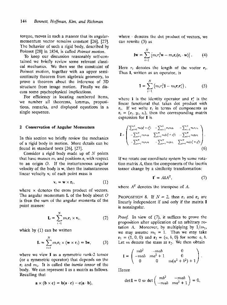


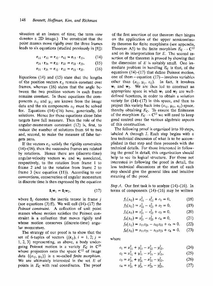

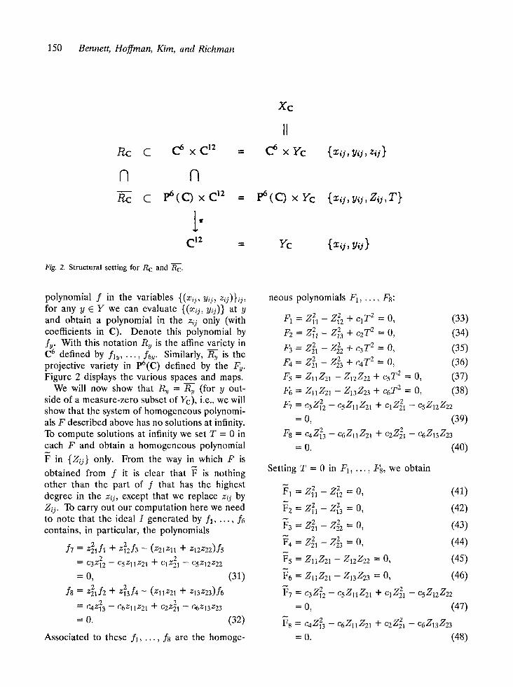


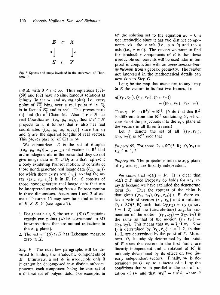


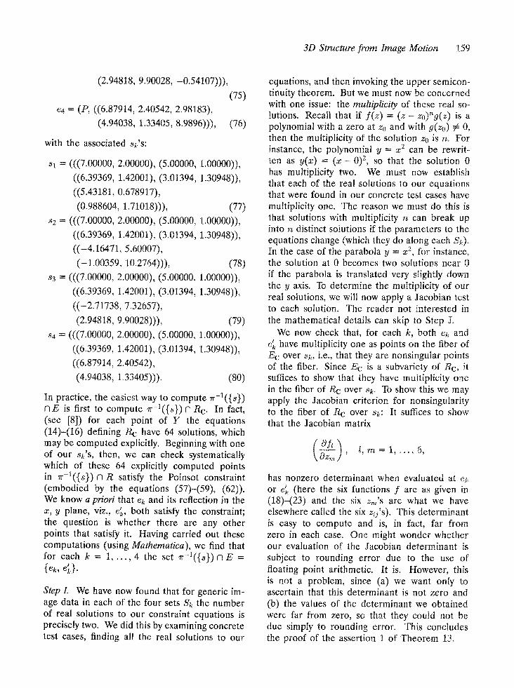


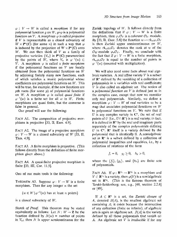


![A novel formulation for determining joint constraint loads during … · 2008. 4. 3. · the optimization-based motion planning method [19]. The determination of constraint loads](https://static.documents.pub/doc/80x56/606f3391fd63ce266f596c65/a-novel-formulation-for-determining-joint-constraint-loads-during-2008-4-3.jpg)


