Prof. Brian L. Evans

Dept. of Electrical and Computer Engineering

The University of Texas at Austin

EE345S Real-Time Digital Signal Processing Lab Fall 2006

Lecture 6

Infinite Impulse Response Filters

6 - 2

Digital IIR Filters

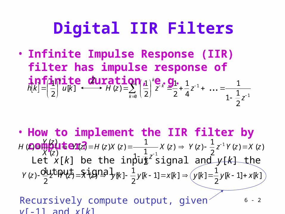
• Infinite Impulse Response (IIR) filter has impulse response of infinite duration, e.g.

• How to implement the IIR filter by computer?Let x[k] be the input signal and y[k] the output signal,

][2

1kukh

k

1

1

0

21

1

1

4

1

2

1

2

1 )(

zzzzH k

k

k

...Z

)()( 2

1)( )(

21

1

1)()()(

)(

)()( 1

1

zXzYzzYzXz

zXzHzYzX

zYzH

][]1[2

1][ ][]1[

2

1][ )()(

2

1)( 1 kxkykykxkykyzXzYzzY

Recursively compute output, given y[-1] and x[k]

6 - 3

Different Filter Representations

• Difference equation

Recursive computation needs y[-1] and y[-2]

For the filter to be LTI,y[-1] = 0 and y[-2] = 0

• Transfer functionAssumes LTI system

• Block diagram representation

Second-order filter section (a.k.a. biquad) with 2 poles and 0 zeros

][]2[8

1]1[

2

1][ kxkykyky

x[k] y[k]

UnitDelay

UnitDelay

1/2

1/8

y[k-1]

y[k-2]

21

21

81

21

1

1

)(

)()(

)()(8

1)(

2

1)(

zzzX

zYzH

zXzYzzYzzY

Poles at –0.183 and +0.683

6 - 4

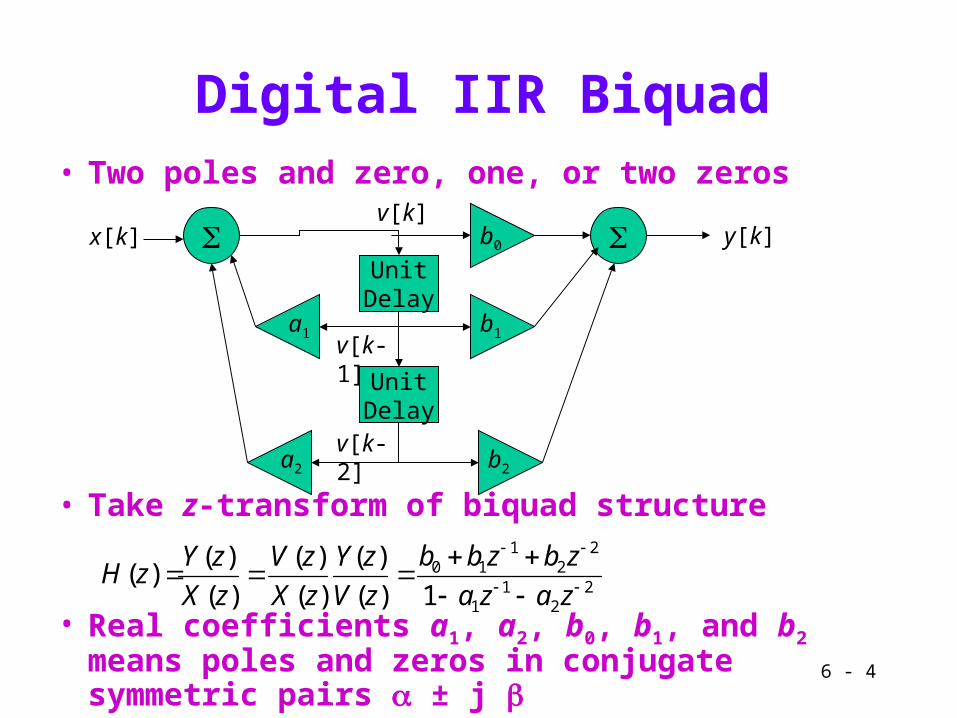
Digital IIR Biquad

• Two poles and zero, one, or two zeros

• Take z-transform of biquad structure

• Real coefficients a1, a2, b0, b1, and b2 means poles and zeros in conjugate symmetric pairs ± j

22

11

22

110

1)(

)(

)(

)(

)(

)()(

zaza

zbzbb

zV

zY

zX

zV

zX

zYzH

x[k]

UnitDelay

UnitDelay

v[k-1]

v[k-2]

v[k]

b2

a1

a2

b1

y[k]b0

6 - 5

Digital IIR Filter Design

• Poles near unit circle indicate filter’s passband(s)

• Zeros on/near unit circle indicate stopband(s)

• Biquad with zeros z0 and z1, and poles p0 and p1

Transfer function

Magnitude response

10

10 )(pzpz

zzzzCzH

10

10

)(

pepe

zezeCeH

jj

jjj

10

10

)(

pepe

zezeCeH

jj

jj

j

Distance from point on unit circle ej and pole location p0

|a – b| is distance between complex numbers a and b

6 - 6

Digital IIR Biquad Design Examples

• Transfer function

• Poles (X) & zeros (O) in conjugate symmetric pairs– For coefficients in unfactored transfer function to be real

• Filters below have what magnitude responses?

Re(z)

Im(z)

XOO X Re(z)

Im(z)

O

OX

X

Re(z)

Im(z)O

O

X

X

1

11

0

11

10

10

10

11

11 )(

zpzp

zzzzC

pzpz

zzzzCzH

lowpasshighpass bandpass bandstop

allpass notch?

Poles have radius r zeros have radius 1/r

6 - 7

A Direct Form IIR Realization

• IIR filters having rational transfer functions

• Direct form realization– Dot product of vector of N +1

coefficients and vector of currentinput and previous N inputs (FIR section)

– Dot product of vector of M coefficients and vector of previous M outputs (FIR filtering of previous output values)

– Computation: M + N + 1 MACs– Memory: M + N words for previous inputs/outputs and

M + N + 1 words for coefficients

MM

NN

zaza

zbzbb

zA

zB

zX

zYzH

1

)(

)(

)(

)()(

11

110

...

N

n

nn

M

m

mm zbzXzazY

01

)( 1 )(

M

mm

N

nn mkyankxbky

10

][ ][ ][

6 - 8

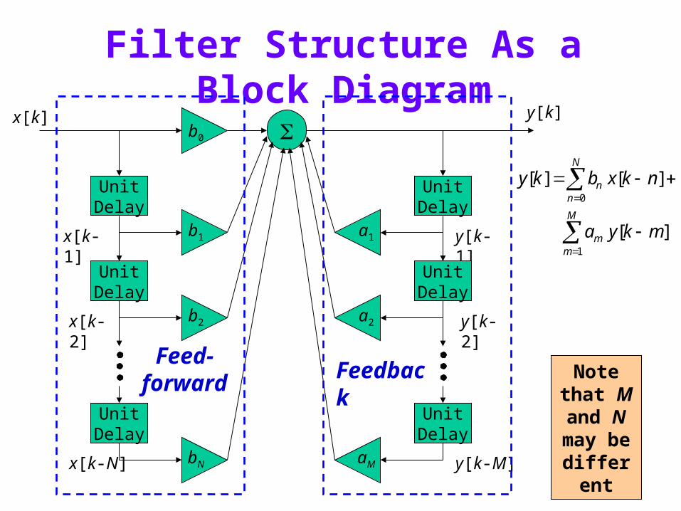
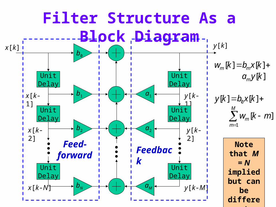
Filter Structure As a Block Diagram

M

mm

N

nn

mkya

nkxbky

1

0

][

][ ][

x[k] y[k]

y[k-M]

x[k-1]

x[k-2] b2

b1

b0

UnitDelay

UnitDelay

UnitDelay

x[k-N] bN

Feed-forward

a1

a2

y[k-1]

y[k-2]

UnitDelay

UnitDelay

UnitDelay

aM

Feedback Note that M and N may be

different

6 - 9

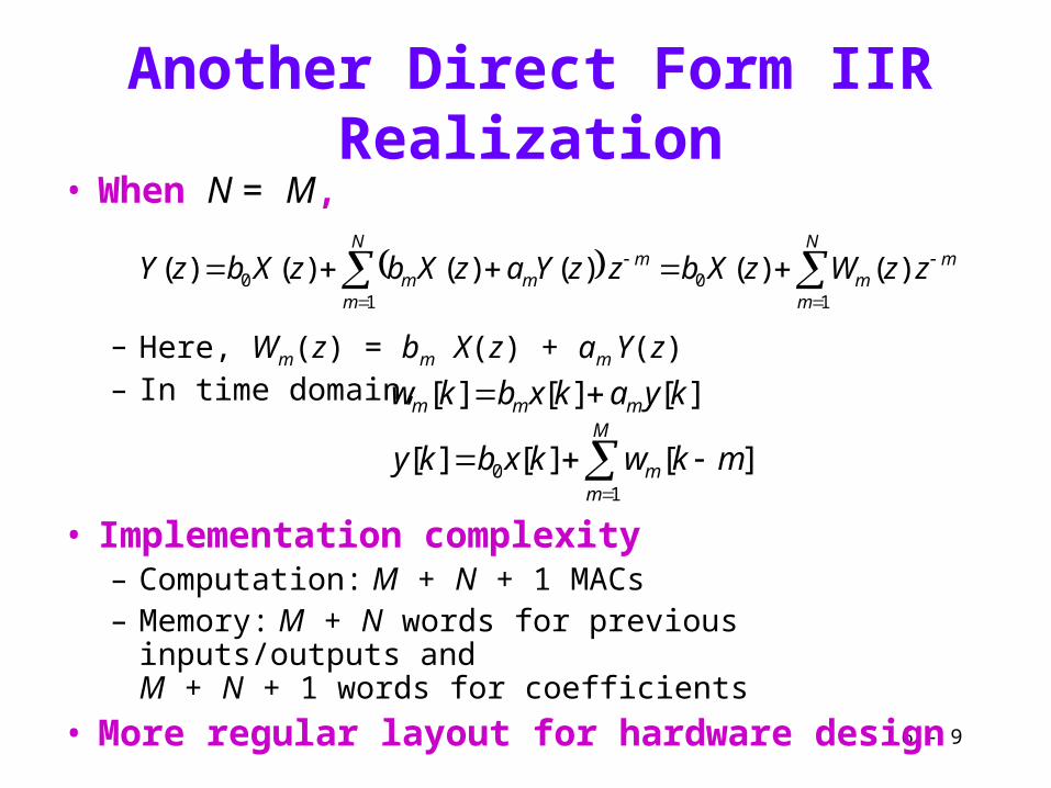
Another Direct Form IIR Realization

• When N = M,

– Here, Wm(z) = bm X(z) + am Y(z)– In time domain,

• Implementation complexity– Computation: M + N + 1 MACs– Memory: M + N words for previous inputs/outputs and

M + N + 1 words for coefficients

• More regular layout for hardware design

mN

mm

mN

mmm zzWzXbzzYazXbzXbzY

)()( )()()()(

10

10

M

mm

mmm

mkwkxbky

kyakxbkw

10 ][][][

][][][

6 - 10

Filter Structure As a Block Diagramx[k]

x[k-1]

x[k-2] b2

a1

a2

b1

y[k]b0

UnitDelay

UnitDelay

UnitDelay

x[k-N] bN

y[k-1]

y[k-2]

UnitDelay

UnitDelay

UnitDelay

y[k-M]aM

Feed-forward

Feedback

M

mm

m

mm

mkw

kxbky

kyakxbkw

1

0

][

][][

][ ][][

Note that M = N

implied but can be different

6 - 11

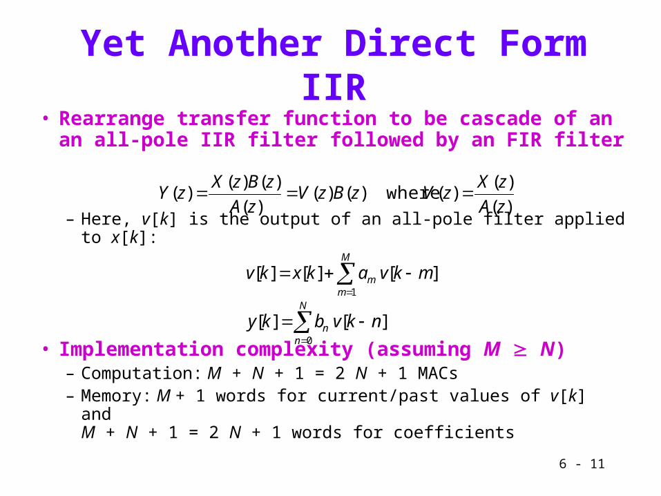
Yet Another Direct Form IIR

• Rearrange transfer function to be cascade of an an all-pole IIR filter followed by an FIR filter

– Here, v[k] is the output of an all-pole filter applied to x[k]:

• Implementation complexity (assuming M N)– Computation: M + N + 1 = 2 N + 1 MACs– Memory: M + 1 words for current/past values of v[k] and

M + N + 1 = 2 N + 1 words for coefficients

)(

)()( where)()(

)(

)()()(

zA

zXzVzBzV

zA

zBzXzY

N

nn

M

mm

nkvbky

mkvakxkv

0

1

][ ][

][ ][][

6 - 12

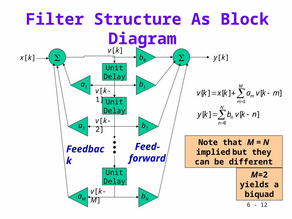
Filter Structure As Block Diagram

x[k]

UnitDelay

UnitDelay

v[k-1]

v[k-2]

v[k]

b2

a1

a2

b1

y[k]b0

UnitDelay

v[k-M]bNaM

Feed-forward

Feedback

M=2 yields a biquad

N

nn

M

mm

nkvbky

mkvakxkv

0

1

][ ][

][ ][][

Note that M = N implied but they can be different

6 - 13

Demonstrations (DSP First)

• Web site: http://users.ece.gatech.edu/~dspfirst

• Chapter 8: IIR Filtering Tutorial (Link)• Chapter 8: Connection Betweeen the Z and

Frequency Domains (Link) • Chapter 8: Time/Frequency/Z Domain Moves for

IIR Filters (Link)

6 - 14

Stability

• A digital filter is bounded-input bounded-output (BIBO) stable if for any bounded input x[k] such that | x[k] | B < , then the filter response y[k] is also bounded | y[k] | B <

• Proposition: A digital filter with an impulse response of h[k] is BIBO stable if and only if

– Any FIR filter is stable– A rational causal IIR filter is stable if and only if its poles

lie inside the unit circle

|][| khn

Review

6 - 15

azza

kuaZ

k

for 1

1

1

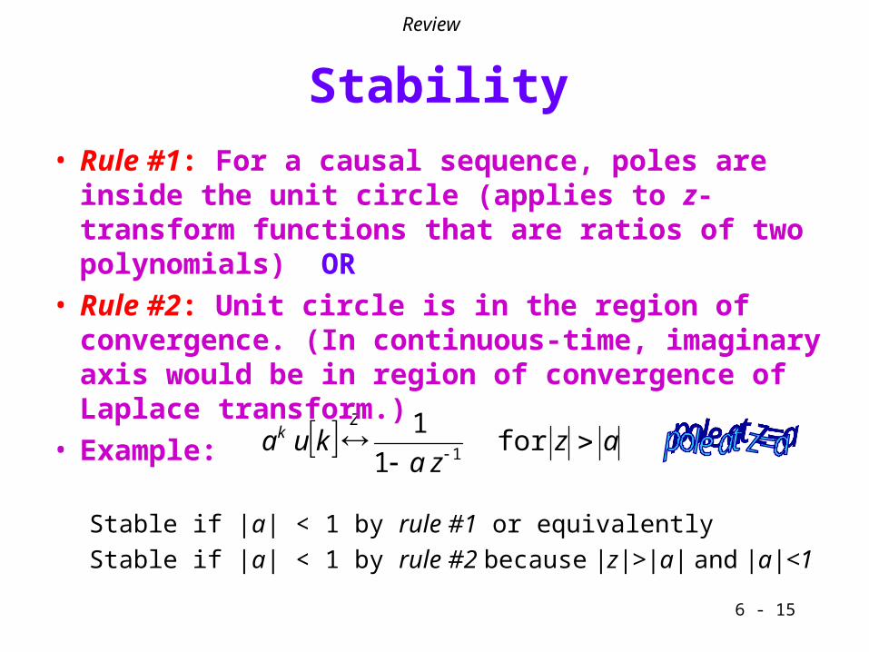
Stability

• Rule #1: For a causal sequence, poles are inside the unit circle (applies to z-transform functions that are ratios of two polynomials) OR

• Rule #2: Unit circle is in the region of convergence. (In continuous-time, imaginary axis would be in region of convergence of Laplace transform.)

• Example:

Stable if |a| < 1 by rule #1 or equivalently

Stable if |a| < 1 by rule #2 because |z|>|a| and |a|<1

Review

6 - 16

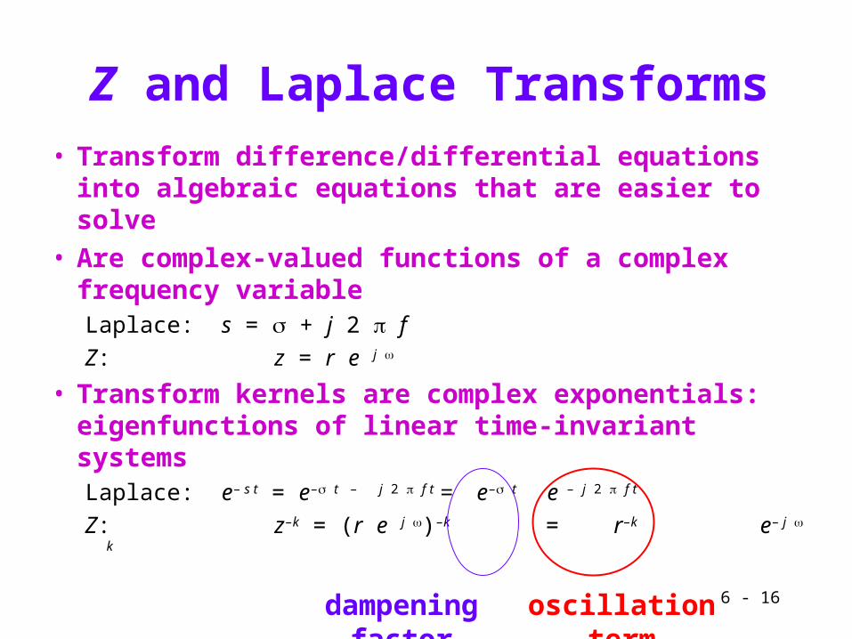
Z and Laplace Transforms

• Transform difference/differential equations into algebraic equations that are easier to solve

• Are complex-valued functions of a complex frequency variableLaplace: s = + j 2 f

Z: z = r e j

• Transform kernels are complex exponentials: eigenfunctions of linear time-invariant systemsLaplace: e– s t = e– t – j 2 f t = e– t e – j 2 f t

Z: z–k = (r e j )–k = r–k e– j k

dampening factor oscillation term

6 - 17

Z and Laplace Transforms

• No unique mapping from Z to Laplace domain or from Laplace to Z domain– Mapping one complex domain to another is not unique

• One possible mapping is impulse invariance – Make impulse response of a discrete-time linear time-

invariant (LTI) system be a sampled version of the continuous-time LTI system.

H(z) y[k]f[k]

Z

H(s) tf~ ty~

Laplace

TsezzHsH |)()(

6 - 18

Impulse Invariance Mapping

• Impulse invariance mapping is z = e s T

Laplace Domain Z Domain

Left-hand plane Inside unit circle

Imaginary axis Unit circle

Right-hand plane Outside unit circle

1

Im{z}

Re{z}

s = -1 j z = 0.198 j 0.31 (T = 1 s)

s = 1 j z = 1.469 j 2.287 (T = 1 s)

1

2

11 maxmax sffω

1

1

-1

-1

Im{s}

Re{s}

fjs 2 lowpass, highpass

bandpass, bandstop allpass, or notch?

6 - 19

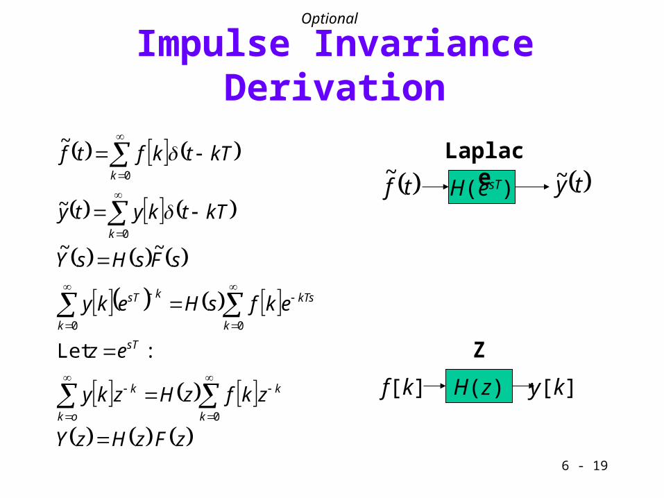
Impulse Invariance Derivation

zFzHzY

zkfzHzky

ez

ekfsHeky

sFsHsY

kTtkyty

kTtkftf

k

k

ok

k

sT

k

kTs

k

ksT

k

k

:Let

~~

~

~

0

00

0

0

H(z) y[k]f[k]

Z

H(esT) tf~ ty~

Laplace

Optional

6 - 20

Analog IIR Biquad

• Second-order filter section with 2 poles and 2 zeros– Transfer function is a ratio of two real-valued polynomials

– Poles and zeros occur in conjugate symmetric pairs

• Quality factor: technology independent measure of sensitivity of pole locations to perturbations– For an analog biquad with poles at a ± j b, where a < 0,

– Real poles: b = 0 so Q = ½ (exponential decay response)

– Imaginary poles: a = 0 so Q = (oscillatory response)

Qa

baQ

2

1 where

2

22

6 - 21

Analog IIR Biquad

• Impulse response with biquad with poles a ± j b with a < 0 but no zeroes:– Pure sinusoid when a = 0 and pure decay when b = 0

• Breadboard implementation– Consider a single pole at –1/(R C). With 1% tolerance on

breadboard R and C values, tolerance of pole location is 2%– How many decimal digits correspond to 2% tolerance?– How many bits correspond to 2% tolerance?– Maximum quality factor is about 25 for implementation of

analog filters using breadboard resistors and capacitors.– Switched capacitor filters: Qmax 40 (tolerance 0.2%)– Integrated circuit implementations can achieve Qmax 80

) cos( )( tbeCth ta

6 - 22

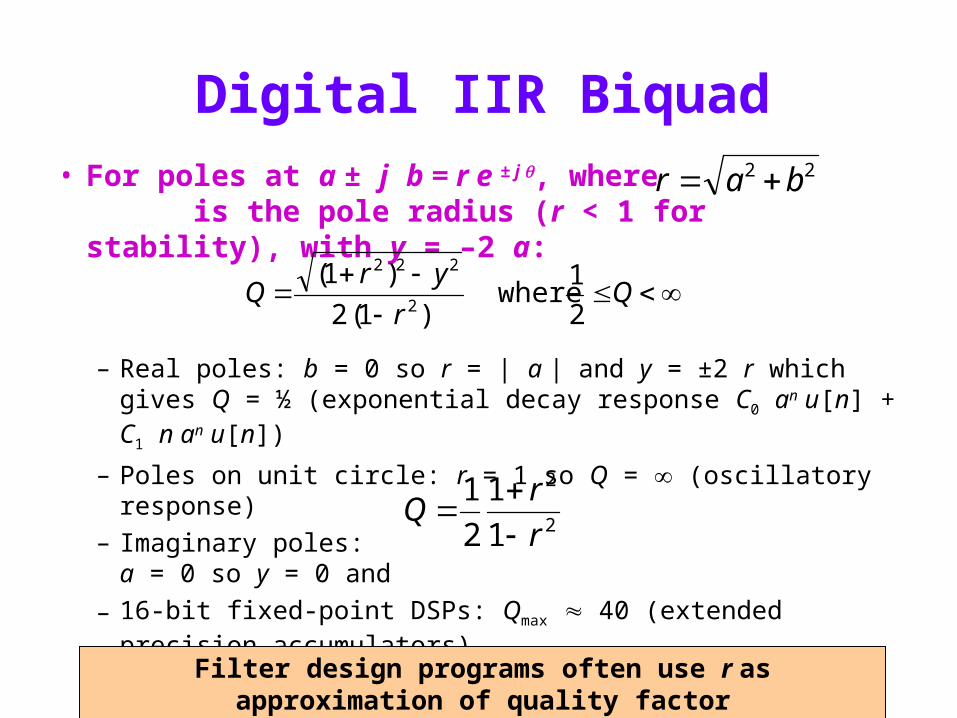
Digital IIR Biquad

• For poles at a ± j b = r e ± j , where is the pole radius (r < 1 for stability), with y = –2 a:

– Real poles: b = 0 so r = | a | and y = ±2 r which gives Q = ½ (exponential decay response C0 an u[n] + C1 n an u[n])

– Poles on unit circle: r = 1 so Q = (oscillatory response)

– Imaginary poles:a = 0 so y = 0 and

– 16-bit fixed-point DSPs: Qmax 40 (extended precision accumulators)

Q

r

yrQ

2

1 where

)1( 2

)1(2

222

22 bar

2

2

1

1

2

1

r

rQ

Filter design programs often use r as approximation of quality factor

6 - 23

Analog/Digital IIR Implementation

• Classical IIR filter designsFilter of order n will have n/2 conjugate roots if n is even or

one real root and (n-1)/2 conjugate roots if n is odd

Response is very sensitive to perturbations in pole locations

• Robust way to implement an IIR filterDecompose IIR filter into second-order sections (biquads)

Cascade biquads in order of ascending quality factors

For each pair of conjugate symmetric poles in a biquad, conjugate zeroes should be chosen as those closest in Euclidean distance to the conjugate poles

6 - 24

Classical IIR Filter Design

• Classical IIR filter designs differ in the shape of their magnitude responses Butterworth: monotonically decreases in passband and

stopband (no ripple) Chebyshev type I: monotonically decreases in passband but

has ripples in the stopband Chebyshev type II: has ripples in passband but monotonically

decreases in the stopband Elliptic: has ripples in passband and stopband

• Classical IIR filters have poles and zeros, except that analog lowpass Butterworth filters are all-pole

• Classical filters have biquads with high Q factors

6 - 25

Analog IIR Filter Optimization

• Start with an existing (e.g. classical) filter design• IIR filter optimization packages from UT Austin

(in Matlab) simultaneously optimizeMagnitude response

Linear phase in the passband

Peak overshoot in the step response

Quality factors

• Web-based graphical user interface (developed as a senior design project) available at

http://signal.ece.utexas.edu/~bernitz

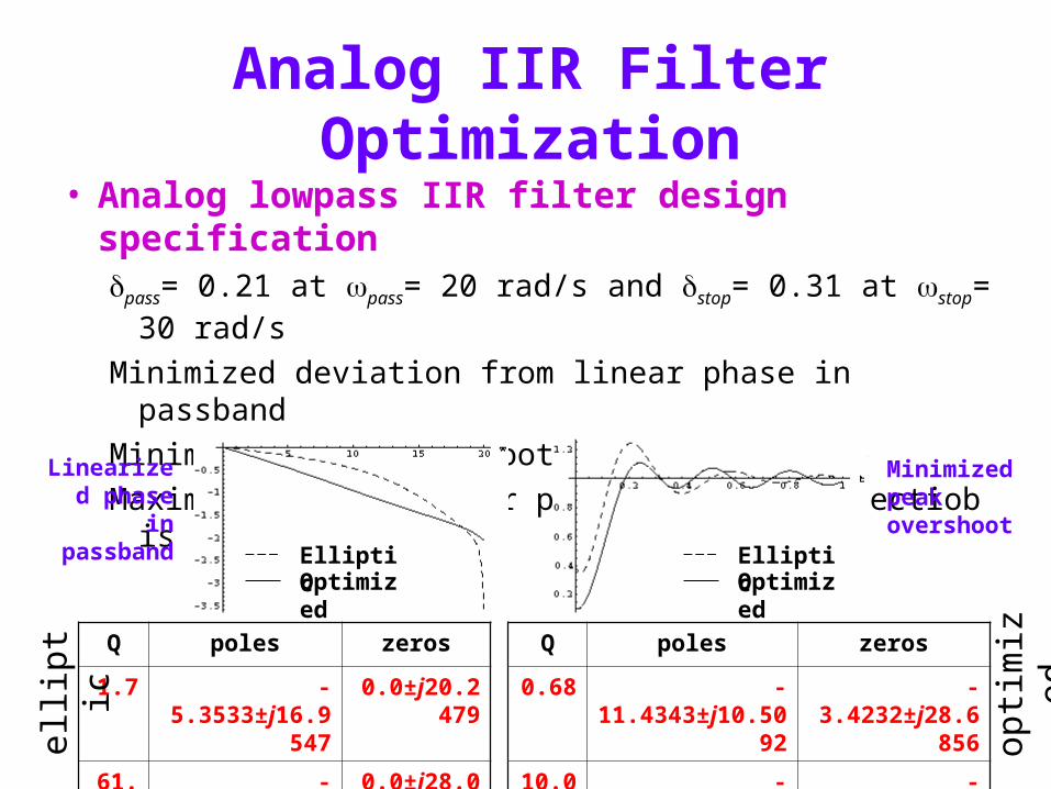
Analog IIR Filter Optimization

• Analog lowpass IIR filter design specificationpass= 0.21 at pass= 20 rad/s and stop= 0.31 at stop= 30 rad/s

Minimized deviation from linear phase in passband

Minimized peak overshoot in step response

Maximum quality factor per second-order sectiob is 10

Linearized phase

in passband

Minimized peak overshoot

EllipticOptimized

Q poles zeros

1.7 -5.3533±j16.9547 0.0±j20.2479

61.0 -0.1636±j19.9899 0.0±j28.0184elli

ptic Q poles zeros

0.68 -11.4343±j10.5092 -3.4232±j28.6856

10.00 -1.0926±j21.8241 -1.2725±j35.5476 opti

miz

ed

EllipticOptimized