1428 IEEE TRANSACTIONS ON INFORMATION THEORY, VOL. 34, NO. 6, NOVEMBER 1988

Infinite Series of Interference Variables with Cantor-Type Distributions

Abstract-The sum of an infinite series of weighted binary random variables arises in communications problems involving intersymbol and adjacent channel interference. If the weighting asymptotically decays at least exponentially and if the decay is not too slow, the sum has an unusual distribution which has neither a density nor a discrete mass function, and therefore cannot be manipulated with usual techniques. The distribution of the sum is given, and the calculus for dealing with the distribution is presented. It is shown that these Cantor-type random variables arise in a range of digital communications models, and exact explicit expressions for performance measures, such as the probability of error, may be obtained. Several examples are given.

I. INTRODUCTION

T H E RANDOM variable 1

j = l

where XI, X,, are independent random variables tak- ing on the values +1 with probability 1/2, arises in the study of digital transmission systems with intersymbol and adjacent channel interference. In a pulse-amplitude-mod- ulated transmission system with additive noise, the output of the receive filter on which the decisions are made is of the form [l]

v ( t ) = 4) + n ( t > (2) where s ( t ) is the superposition of the received pulses

03

s ( t ) = c X , h ( t - J T ) (3) j = - w

and n ( t ) , the additive noise, is often Gaussian. The output of the receive filter is sampled at time to to yield the statistic on which the decision about a particular bit, say X,, is made:

03

Y = c X - j p j + N . (4) j = - m

Manuscript received January 15, 1988; revised July 5 , 1988. This research was supported by the Natural Sciences and Engineering Re- search Council of Canada under Grants A3391 and A2151. The initial part of this work was presented at the IEEE International Symposium on Information Theory, Ronneby, Sweden, June 1976.

P. H. Wittke and W. S. Smith are with the Department of Electrical Engineering, Queen's University, Kingston, ON, Canada K7L 3N6.

L. L. Campbell is with the Department of Mathematics and Statistics, Queen's University, Kingston, ON, Canada, K7L 3N6.

IEEE Log Number 8824872.

Then the coefficients system response function h (t),

are regularly spaced samples of a

p j = h ( t , + j T ) . ( 5 ) The decision about a particular bit would be made on the basis of the sign of Y, that is, X,=1 if Y 2 0 , and X, = - 1 if Y < 0. The decision variate can be written

Y = X,p, + Z; + Z,.I + N ( 6 )

where 2; is given by (1) and Z: is a similar sum over negative indices. In the case of a causal system model, the second inteference variable vanishes, and the probability of error is given by

P, = Pr( Y = Po + Z , + N < OlX, =1)

with Z, of the form (l), and p, = h ( t , + JT). Otherwise, a pair of interference variables appears in (7).

For almost all systems the distribution of Z , has not been known, and so bounds and computational procedures have been used to evaluate error probability. For a discus- sion of the techniques and a comprehensive bibliography, see the paper by Helstrom [2] which presents a new numer- ical technique.

Other important communications problems exist in which infinite sums of interference variables arise but not in a straightforward additive fashion as in (7). For exam- ple, to obtain constant envelope modulations that meet stringent requirements on the out-of-band radiative power, shaping the baseband modulating pulses has been incorpo- rated with modulations such as minimum shift keying (MSK) and intersymbol interference results. MSK where the baseband pulses are shaped by a Gaussian filter results in GMSK [3], [4]. In mobile applications a noncoherent detection may be necessary, in which case the performance is dependent in a nonlinear fashion on the intersymbol interference infinite sum.

The purpose of this paper is to present the distribution and properties of the random variable Z , for system functions that asymptotically decay at least exponentially as would be encountered in a range of models for commu- nications systems and where the rate of asymptotic decay is not too slow. These systems give rise to an unusual class of random variables which are neither continuous nor discrete and cannot be manipulated in the usual way. Nevertheless, a calculus for dealing with them can be

(7)

0018-9448/88/llOO-1428$01.00 01988 IEEE

W I ~ K E et al.: INFINITE SERIES OF INTERFERENCE VARIABLES 1429

developed, and exact explicit expressions for performance measures such as P, result.

In [9] Rice presented a recursive equation for the distri- bution function. Huzii and Sugiyama [lo] have derived a related set of functional equations whose solution tends to

11. HISTORICAL BACKGROUND the distribution function of intersymbol interference under

The cases in which the infinite sum (1) has been dealt with directly are as follows. A number of the results are due to Rice who, we understand, had an early interest in the problem. For pj =l/J, Rice [5] has evaluated the distribution of Z, numerically and given asymptotic ex- pressions for the tails of the distribution. This particular random sum arises in a pulse transmission system with a rectangular system function and timing error. The other case which has yielded results is the random geometric series where pj = PJ. A survey paper which considers the application to the intersymbol interference problem has been presented by Hill and Blanco [6]. Hill developed a computational technique [7] for calculating the effects of intersymbol interference for the geometric case. Also, in cases where the intersymbol interference was not strictly geometric, Hill and Blanco have estimated the probability of error from that of an approximating geometric series [SI. They point out that Rice reported on the problem in an unpublished memorandum in 1957 [9], summarizing results he attributes to others and providing new ones as well.

Rice’s memorandum [9] on random geometric series where the binary variables can take values 0 or 1, is related to the response of a resonant circuit to a train of random pulses, as might occur in timing recovery for pulse-code modulation (PCM) systems. Results were presented on estimation of the distribution and normal law approxima- tion as j3 -1. He gave expressions for the moments and semi-invariants of Z,, where the binary variables are 0 or 1 and 2, is defined by (8) below. An explicit expression for the distribution function of 2, was given for p =l/fi, and a derivation was presented of the result that for p = 2T1lK, K an integer, the distribution function of Z =

(l-p)Zo is

F , ( x ) = A(1+ x ) ~ , for x s1-3p/2

where

A = (1 - 2-1/K) - [2-(3K+ 1)/2 ] / K ! .

the assumption that the pulse samples decrease exponen- tially. These recursive forms will be used in the distribu- tion function evaluation below.

The sum (l), can be viewed as resulting from an infinite series of convolutions of binary or Bernoulli random vari- ables. There is a mathematical literature [11]-[13] on infi- nite convolutions of binary random variables. It is known [ l l ] that the distribution function of the sum is continu- ous. However there are cases where it is not absolutely continuous and so the distribution is singular, without a density function. The main concern in the mathematical work has been with the conditions under which the distri- bution function is singular or absolutely continuous. The problem is not yet completely resolved. The cases where the distribution is known explicitly are few. For the geo- metric series and p = 1/2, the distribution is uniform [14]. For p an integer root of 1/2, the distribution was given in 1957 in unpublished work by Rice, as mentioned before. Lucky et al. [15, p. 601 point out that for /3 <1/2 the distribution is singular and indeed the distribution for /3 = 1/3 or /3 = 1/4 is used in probability and analysis as a construction of a singular random variable or a distribu- tion function that is continuous but with a zero derivative almost everywhere [16]. Thus the integral of the derivative does not yield a distribution function, let alone the original function. Such a distribution function is sketched in Fig- ure 1.

111. RANDOM SUMS WITH CANTOR-TYPE DISTRIBUTIONS

Let m

‘ k = c x j p j (8) j = k

and

j = k (9)

Here the binary variables can take values f 1. where it is assumed that the series (9) is convergent. Since

, .: I’ , I .;-.--:- - 1 12 - -. -

1 -1 I2 0 112 1 L

R1

Example of Cantor-type distribution function Fig. 1.

1430 IEEE TRANSACTIONS ON INFORMATION THEORY, VOL. 34, NO. 6, NOVEMBER 1988

TABLE I SOME CHANNELS YIELDING CANTOR-TYPE RANDOM VARIABLES

Bandwidth for Z,,, to be Cantor Type i.e., B,, > R r + l for all n 2 m tn 8,

for all m if /3 <1/2 or B T > 0.11 for all m if /3 < 1/2 or BT > 0.11 for m = 0 if B < 0.262 or BT > 0.137

m = 1 /.? < 0.358 BT > 0.105 m - w 8 < 1 / 2 BT>0.071

for m = 0 if < 0.187 or B T > 0.172 m = 1 /3 < 0.327 BT > 0.114

form = 0 if /? < 0.188 or BT> 0.136 m = 1 B < 0.289 BT > 0.101 m + w /.3<1/2 BT>0.056

for m = 1 if /3* < 0.8503 or BT > 0.0755 m = 2 /3 * < 0.8975 BT > 0.0616

for m = 1 if /3* < 0.840 or BT > 0.0784

~

Notes: 1) /3 = exp(- aT) and B* = exp(- Cr’T’). 2) h ( t ) for the last entry is the differential phase change for GMSK, where f ( t ) = rq(fiat)-exp(- a’t’)/2&, and q ( . ) is defined after (39).

the X, in (1) can take on the values k 1 with equal probability, there is no loss in generality in assuming ?he p’s to be positive. The summability of the coefficients pj (9) implies that they are also square-summable which is the necessary and sufficient condition that the infinite series of convolutions of the binary or Bernoulli distribution func- tions converges to a distribution function [l l] . It is known [U], [13] that under the condition E:-#; < 00, the infinite convolution of binary distribution functions converges to a distribution function that is continuous and “pure” in the sense that it is either absolutely continuous or singular but not a composition of the two. Furthermore, if

/3,, > R,+l for all n 2 m, (10) the distribution function of 2, increases on a set of measure limn - ,2“R + 1. Thus if

lim 2”Rn=0, (11) n + c a

the distribution of Z,,, is singular and in addition of the Cantor type, which means it takes on constant values except on a set of measure zero. (There are other types of singular distributions.) Equation (10) implies that the B ’ s are monotone decreasing for all n 2 m, and /In = 0(2 - ” ) . Equation (11) is satisfied if p,, = O ( p ” ) for some p <1/2.

Suppose (10) and (11) hold or the coefficients Is, can be reordered into a series for which they hold. In this paper, the distribution function of 2, will be given, and its statistical properties will be found. Methods for dealing with these variables as they occur in communications problems will be presented. However, first let us examine a range of channel models that yield Cantor-type distribu- tions. Error rates for some particular examples of these models have been estimated previously using bounds [17] and numerical techniques [6] .

Table I shows a selection of channel responses h ( t ) which, when sampled, yield a Cantor variable Z,. The coefficients b, are given by

p j = h ( t 0 + j T )

where to has been chosen to yield a maximum bo which is taken to be the magnitude of the desired signal variable. Note that the channel response h ( t ) is assumed to be causal, i.e., h ( t ) = 0 for t < 0. (The noncausal case can be treated as well, although the results are more complicated. In particular, where a single Cantor variable now appears there would be a pair of Cantor variables, and the results in Section IV involving double summations would involve summation over four indices.) In the causal case, the intersymbol interference variable is Z,, which can be scaled as desired without altering the type of variable. In general, it is found that the variables are Cantor-type for all normalized bandwidths BT, greater than the constant shown in the table. The minimum bandwidth depends on the particular form of the channel response h , and the sampling time to. Single-sided bandwidths to the 3-dB point were used. p ( t ) is a rectangular pulse of unit ampli- tude over the interval (O,T), and an asterisk indicates convolution. For the case where h ( t ) is of the form p ( t ) * f( t), which corresponds to transmission with a pulse input, the single-sided 3-dB bandwidth of f ( t ) is presented in the table. For a channel response of the form t ” exp ( - at ) the results were obtained from an identity for the remainder R i . Let

m

R i = j”,SJ. (13) j = k

Then

This yields a polynomial of degree k which can be solved for the permissible range of p. For example, for the response a2t exp( - at),

- ( (3+m + r , / ~ ) - ~ ) ~ - 8 ) ~ ’ ~ ] / 4 . (15)

1431 WIlTKE et d. : INFINITE SERIES OF INTERFERENCE VARIABLES

If the channel is noncausal but the response h ( t ) yields a Cantor variable for t > 0 and another Cantor variable for t < 0, the distribution of Z can be treated as the convolu-

For example,

y 1 , 1 = - P1

y 2 , 1 = - P1- P 2

Y 1 , 2 = + P1,

Y 2 , 2 = - P 1 + P2 tion of two Cantor-type variables. If the channel response is an exponentially damped sinusoid Y2.3 = + P 1 - b2 Y 2 , 4 = + P 1 + P 2 9

fin = P" sin ( n UT + $11, (16) and so on. Again, from a consideration of the separation between the values that can be taken by the partial sum in (19) and from the inequality P,, > R,+l , Fzl is defined by (20) except on a set of measure 2"+1Rn+1. This goes to zero under assumption (I1) as

the distribution of Zk can be expressed as a convolution of Cantor variables when oT is a rational fraction of v. The complexity involved in treating this case or the number of convolutions varies directly as the length of the period of --* 03. Th

the sine wave. 2 J + 1 F Z I ( X ) = 0, x < ~ j , 1 - ',+I= - ' 1

=1, Y J , l - PJ+l < < yJ,l + pJ+l

= 2, Y J , 1 + R J + l < < Y J . 2 - R J + l

If conditions (10) and (11) do not hold for all n, but only for n greater than or equal to some integer m, then

finite sum of variables with the Cantor Z,. However, the amount of work involved in dealing with the convolutions

the distribution can be treated as the convolution of a

increases dramatically with m, even for small m. = 2( - 9 Y J , k - 1 + J + 1 < < Y,, k - J + 1

IV. DISTRIBUTION FUNCTION EVALUATION

In t h s section a technique for evaluating the distribu- tion function for distributions satisfying (10) and (11) will be presented. To simplify the notation, let us assume these conditions are satisfied for m =l . This restriction will be removed later.

Since Zk = XkPk + Zk+l, there is a recursion expression for the distribution function

FZk( ) = ( 1 / 2 ) [ FZk+l( + P k ) + FZk+l( - P k )] . (I7) Since Pk > Rkt l , and Xk = f 1 each with probability 1 / 2 , it follows that

X < - R k

F Z k ( X ) = 1/29 - P k + R k + l < < P k - R k + l . [:: X > R k

(18)

(19)

The variable Z, can be written n

' 1 = C x1Pi + Z n + 1 1 = 1

and can be conditioned on the 2" values taken on by the partial sum in (19),

2"

F Z ~ ( X ) = 2-" C ~ z , + , ( x + Y n , , ) (20) I =1

where y , , , can take on the 2" values: f P1 f P2 f . . f i n . Since P,, > R n t l , the y,,, can be ordered in increasing value simply by relating the & coefficients to the binary expansion of i . Let

E = (a , ,a2 , - ,an) (21) be the binary expansion of the integer i - 1, where leading zeros have been retained. Then

n

y n , i = ( 2 a k - l ) P k * (22) k = l

Y J , ~ J - ' + R ~ + l = < x, = 2 J + '

k = l 2 J , j = O , 1 , 2 , * * (23 )

where yo,l has been defined as zero and

~ j = P j - R j + l . (24)

The segments of the distribution functions (23) can be written more concisely. Let us define the sets A = ( R , , 00)

and B = (- CO, - R,) and the sequence of sets

k = ( Y n - 1 , k - pn 3 Y n - 1, k + P n ) , k = 1,. ' ' 7 . 2"-'

(25 )

It can be shown, although the demonstration is tedious, that Fzl is defined by (23) over

n + l 2 J - I

U U ' J , k ? j = 1 k = l

and all C J , k are disjoint. For the purposes here, it is sufficient to note that for a particular j the Fstribution function is obviously defined by (23) over UFilCJ, k with

2J-1

= ( 2 k - 1 ) 2 - J 1 ( q , k ~ x ) (26) k = 1

where the indicator function of a set C J , k is defined by

By (25) and th,e disjointness of the sets c , , k , the Lebesgue

00 2 J - 1

measure of U : = , C j , , is 2Jpj. Thus the measure of

'= U U q , k j = l k = l

1432 IEEE TRANSACTIONS ON INFORMATION THEORY, VOL. 34, NO. 6 , NOVEMBER 1988

is W

p(c) = 2JPj. j = 1

From (9), quently,

= R j - R j + l , and so pj = R j - 2 R j + 1 . Conse-

n n

2Jpj= ( 2 J R j - 2 J + ' R . J + 1 ) = 2 R 1 - 2 n + 1 R , + 1 . ;=l j = l

By the hypothesis that (11) holds, 2n+1Rn+1 + 0 as n + M.

Thus

P ( C ) . = 2 4 . Since C is a subset of the interval (- R I , R , ) and since Fzl is constant on A , B , and each interval c J , k , Fzl is a distribution function of the Cantor type, as described by Feller [18, pp. 35-36]. Fzl is constant almost everywhere and, except on a set of Lebesgue measure zero, is given by

m 2 J - l

B. Moments and Characteristic Function

Integration by parts (29) cannot be applied directly to obtain the general nth moment E { Z " } , as g ( z ) = Z" is unbounded. Rather, a lemma given by Feller [18, p. 1481 can be applied. It states that, for any a > 0,

Jo"nF(dz} = a / m z " ' [ l - 0 F ( z ) ] d z , (31)

in the sense that if one side of the equation converges, so does the other side. An analogous result over (- M,O] can be derived as

- ~ ) ~ F { d z } =a/' ( - z ) * - ' F ( z ) dz . (32) /-om( - 0 3

From the symmetry of the distribution function F( z ) =1- F( - z ) (33)

and (31) and (32), it follows that the odd order moments are zero. For n even,

V. THE CALCULUS OF CANTOR VARIABLES

Since the Cantor-type random variables are singular, the conventional calculus which is used with discrete or con- tinuous random variables cannot be applied. However, results presented by Feller [18, ch. IV] on probability measures and spaces can be applied to obtain a calculus for these distributions as follows.

A. Expectation

In communications problems, commonly there is some function g ( Z ) , such as an error performance, that can be obtained given or conditioned on an interference variable Z , which in this case is a Cantor variable. Note that for ease of notation in the general results, the subscript on Z will not be indicated. It is desired to find overall

m 2 J

= 2 R ; - ( & - R 2 ) " - ( 2 k - 1 ) 2 - J J = 1 k = 2 1 - ' + 1

* [ ( Y J , k + p J + l ) " - ( Y J , k - PJ+ 1 ) "1 ' (34)

Similar considerations can be used to find the characteris- tic function

Mzl( j u ) = lm d""F { dz } --M

= COS uR, -COS U ( p1 - R2) 2'

+ f ( 2 k - 1 ) 2 - j J = 1 k = 2 1 - ' + 1

where the notation of Feller F { d z } has been used to indicate the probability measure induced on the real line

that if g is bounded and has a continuous derivative g', then for an arbitrary distribution function F, integration by parts is possible

C. Conuolution of Continuous and Cantor Variables

occur with additive noise such as Gaussian. For example, in the pulse-amplitude~modulated transmission model con- sidered in the Lntroduction, the decision variable is of the

by the distribution function F. shows [18, P. 148i In linear band-restricted channels, interferences usually

form r = p , + w

- g ( a ) F( a ) - Jbg'( z ) F( z ) dz . (29) where a

Thus, for 2, a Cantor variable W = DZ,+ N . ( 36)

In (36), the constant D has been introduced to allow a variation of peak distortion [15 , p. 661, DRJP,. Po is the sample value of the pulse being detected, and N is a Gaussian random variable of mean zero and variance u2. Note that in the results that follow, thereis no limit on the

m 2J-1

- 1 k = 1 E ( g ( Z 1 ) ) = g ( R , ) - c c ( 2 k - W '

. [ g ( ~ , - l , k + p ~ ) - g ( y , - l . k - ~ ~ ) l . (30)

WITTKE er U/ . : INFINITE SERIES OF INTERFERENCE VANABLES 1433

peak distortion for the results to hold, as there has been in much of the work on intersymbol interference. The distri- bution function of W is given by [18, p. 1421

F , ( w ) = /" Fzl ( D - ( w - x ) ) dF, ( x ) . (37)

Since N is a continuous random variable, after a simple change of variable

F , ( w ) = D/- . Fzl ( x ) f , ( w - Dx ) dx .

M

00

(38) 03

This integral is absolutely convergent and so may be written as a sum of integrals over the sets on which Fzl is defined by (27):

F,(w) = D / m f , , , ( w - D x ) d x RI

m 2 J - I

+ D(2k -1)2-J f,(w - D x ) dx J =1 k =1 Lk

= q( 0-1( R,D - w)) m 2 J - 1

1 (2k-1)2-'Q(C1,k,w) (39) j = 1 k = l

where

Q = 4( U-'[ D(Yj-1,k - P,) - w])

- q( '-'[ D(y~- l ,k + w]) and

q ( x ) = ( 2 ~ ) - ' / ~ l ~ e x p ( - t2/2) d t .

The probability of error for a binary transmission sys- tem in Gaussian noise and interference can be obtained directly from F,. If the received signal levels are +bo with probability 1/2 and successive bits are statistically independent, the probability of error is given by

P, = Pr( Po + W < OIXo =1)

=F,(-Po), (40) whch can be evaluated by calculating (39) with w = - Po.

In Sections I11 and IV it was assumed for simplicity that conditions (Io) and i l l ) hold for m =I. Now suppose they hold for an arbitrary m . Then we can form a random variable

ffl-1

w=w+ x,p, (41) J = 1

where W is the sum of a Gaussian and a Cantor random variable as before. The probability of error is given by

* I t - '

p, = 2-m+' c ~ , ( - , 8 0 - I d (42) k = I

where I k takes on the 2"-' possible values that the sum of the X,P, can take on. However, problems that require the

use of (42) become untractable for large m , for the compu- tation time required grows exponentially with m.

VI. EXAMPLES

Examples will be given to indicate the application of the results on Cantor variables to data transmission problems.

A . Additive Intersymbol Interference

Hill and Blanco [6], [8] have considered the random geometric series where p, = P J in (l), and the series is summed from 0 to 00. They consider the application to the calculation of the probability of error in digital transmis- sion systems with additive intersymbol interference, and let the intersymbol interference be

Z = D* (1 - B ) Zo (43)

with pJ=,8J . The constants D* and (1-,8) have been introduced so that the value of D* gives the peak distor- tion which can be set according to the overall magnitude of the intersymbol interference. Note that there is no limit on the value of D* for which the theory applies. They have used a computational technique [7] to evaluate the proba- bility of error (7) and have presented results [6] for N an additive Gaussian variable and for a range of values of ,8 between zero and one. The results of Section IV-C apply for 0 I ,8 <1/2, where a direct comparison with their results can be made.

Error probability has been evaluated using (40) and (39) for a range of values of ,8 and D*. The desired pulse amplitude Po has been set to one, and the scaling parame- ters are related by

D = D*(1- /?)//I. (44)

Early results were obtained on a programmable hand calculator with the series (39) truncated at j = 4 . More recent calculations have been carried out with truncation at j = 5,6,7. The particular choice has not been critical either in terms of accuracy of the results or ease of computation. Values of 6 and 7 have been used when the ,8, decay most slowly.

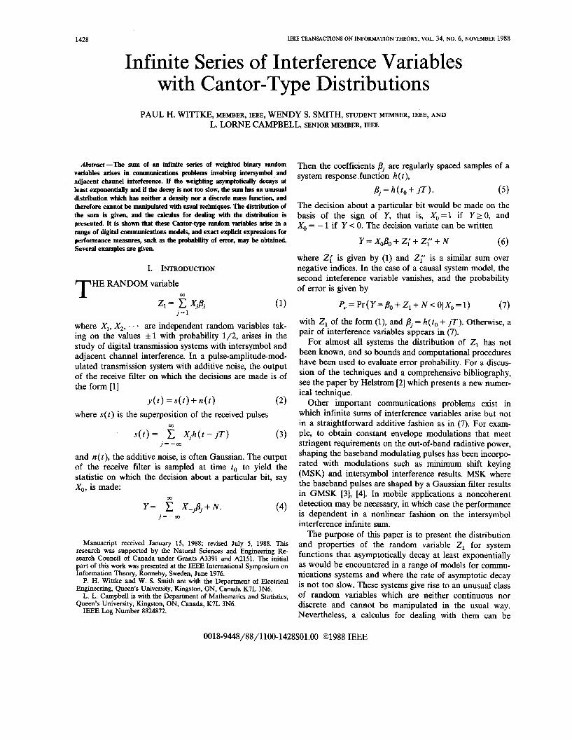
Results for ,8 = 0.3 are presented in Fig. 2. Here the series was truncated at j = 6. The same calculation trun- cated ai j = 5, ~ s u k e d in ii dtrfference in atmosi the fifth least significant figure. The calculations are in close agree- ment with the computational results in [6, p. 3321.

Equations (39) and (40)can he used to evaluate mm performance as a function of channel parameters such as bandwidth or timing offset, for the channel models indi- cated in Table I. As an example, the probability of error is presented in Fig. 3 as a function of bandwidth BT, for transmission of rectangular pulses of duration T s, in additive Gaussian noise with double-sided spectral density N0/2 W/Hz. Reception is by a single-pole low-pass filter with single-sided 3-dB bandwidth B Hz, sampled every T s. The signal-to-noise ratio (SNR) r = A 2 T / N o . For each r, the choice of bandwidth that is the optimum

IEEE TRANSACTIONS ON INFORMATION THEORY, VOL. 34, NO. 6, NOVEMBER 1988

SNR (dB)

Fig. 2. Error probability for PAM transmission in Gaussian noise and geometric interference with /3 = 0.3.

BANDWIDTH BT

0 ; : ' 1 2 3

- 1 6

-18

Fig. 3. Error probability as function of bandwidth ET for pulse trans- mission through single-pole filter.

compromise between noise and intersymbol interference is evident.

B. Noncoherent Detection of FSK

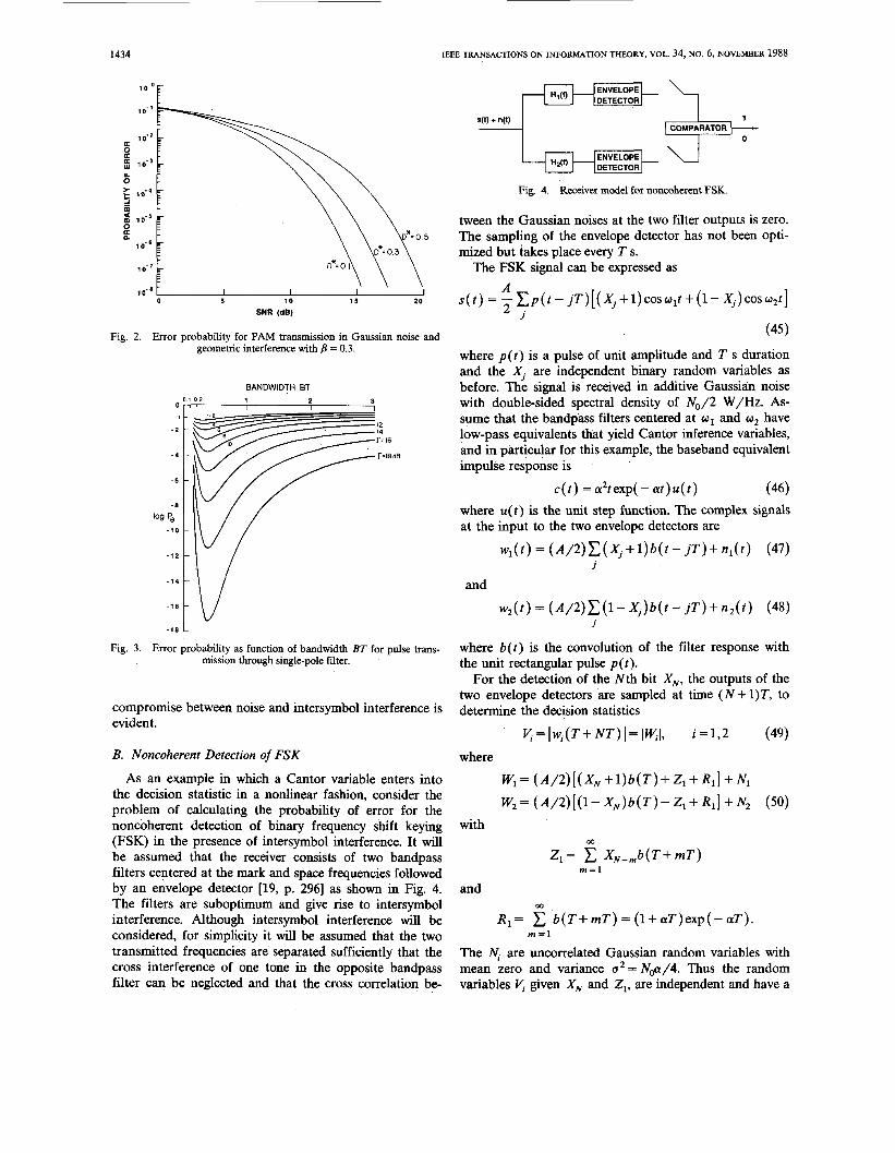
As an example in which a Cantor variable enters into the decision statistic in a nonlinear fashion, consider the problem of calculating the probability of error for the noncoherent detection of binary frequency shift keying (FSK) in the presence of intersymbol interference. It will be assumed that the receiver consists of two bandpass filters centered at the mark and space frequencies followed by an envelope detector [19, p. 2961 as shown in Fig. 4. The filters are suboptimum and give rise to intersymbol interference. Although intersymbol interference will be considered, for simplicity it will be assumed that the two transmitted frequencies are separated sufficiently that the cross interference of one tone in the opposite bandpass filter can be neglected and that the cross correlation be-

+ n@) _i COMPARATOR - &-+ DETECTOR

Fig. 4. Receiver model for noncoherent FSK.

tween the Gaussian noises at the two filter outputs is zero. The sampling of the envelope detector has not been opti- mized but takes place every T s.

The FSK signal can be expressed as A

s( t ) = - p ( t - j T ) [ ( x, + 1) cos w,t + (1 - x,) cos w,t ] 2 J

(45)

where p ( t ) is a pulse of unit amplitude and T s duration and the XJ are independent binary random variables as before. The signal is received in additive Gaussian noise with double-sided spectral density of N, /2 W/Hz. As- sume that the bandpass filters centered at w1 and w2 have low-pass equivalents that yield Cantor inference variables, and in particular for this example, the baseband equivalent impulse response is

c ( t ) = a2texp( - a t ) u ( t )

w l ( t ) = (A/2)C(X, +w - m+ n l w (47)

w z ( t > = ( A / 2 ) C ( l - X , ) b ( t - j T ) + n , ( t ) (48)

(46) where u ( t ) is the unit step function. The complex signals at the input to the two envelope detectors are

J

and

J

where b ( t ) is the convolution of the filter response with the unit rectangular pulse p ( t ) .

For the detection of the Nth bit X,, the outputs of the two envelope detectors are sampled at time (N + 1)T, to determine the decision statistics

v; = I w, ( T + NT ) I = I w, I, i = 1,2 (49) where

Wl = (A/2) [ ( X, + 1) b ( T ) + Zl + R,] + Nl

W, = ( A / 2 ) [(l- X,)b(T) - Z , + RI] + Nz (50) with

W

z,= X, - ,b (T+mT) m = l

and W

R l = b ( T + m T ) = ( l+aT)exp( -aT) .

The N, are uncorrelated Gaussian random variables with mean zero and variance u2 = N , / 4 . Thus the random variables v; given X, and Z,, are independent and have a

m = l

1435 WITTKE et al.: INFINITE SERIES OF INTERFERENCE VARIABLES

conditional Ricean density [19, p. 2971

PV,(U,lZl? x,=1> = ( ~ , / ~ z , " P [ - ( ~ f + w s f ) / 2 ~ 2 ]

4. The number of terms is determined by the accuracy required at the highest signal-to-noise ratios. To obtain accuracy to three significant figures, a J,, of eight was required. This curve is not plotted in Fig. 5 as it would not be distinguishable from the curve for J,, = 4. Signifi- cantly fewer terms are required to achieve similar accuracy at larger bandwidths. In particular, BT = 0.6 requires J,, = 4; BT = 1, J,, = 2; and BT = 2, J,, = 1. Fig. 6 shows

*'o(ufws8/u2) ( 5 1 ) where Io is the zero-order modified Bessel function, and

ws, = ( A / W - R l + Zl)

e,= ( A / 2 ) ( R , - z,>. loo The probability of error may then be obtained from

[19, p. 5871 Pr (error I Z , , X, = 1)

= Pr ( V, > V,(Z, , X, = 1) = p:( Z , )

= Q (6,fi) - (1 / 2 ) exp [ - ( a + b ) / 2 ] Io (a ) ( 5 2) where a = r( R, - Z,)2/aT, b = r ( 2 - R , + Z,)'/aT, Q is Marcum's Q-function, and the SNR r = A2T/2No. Since Pr (error I X , = 1) = Pr (error 1 X, = - l),

P e = E=,{ P: 1. (53)

Finally, since p: is bounded and is a continuously differ- entiable function of Z,, (30) can be used to give

00 2 J - l

P e = p : ( R l ) - C C (2'-1)2-' j = 1 k = l

. [ P : ( Y , - l , k + P,)- P : ( Y , - l , k - P , ) ] . (54)

The probability of error has been plotted as a function of SNR in Fig. 5 , where the infinite sum of (54) has been truncated at j = JmW. This particular example is for a

0.4. Curves are shown for values of J,, ranging from 0 to filter with normalized double-sided 3-dB bandwidth BT =

SNR IN DE

Fig. 6 . FSK error probability as function of SNR with bandwidth parameter.

loo F

SNR IN DB

Fig. 5. Error probability for FSK as function of Jma, number of terms in series.

l o o

/ SNR = 14 DB

.---'-: I j _

NORMALIZED IF FILTER BANDWIDTH, BT

Fig. 7. FSK error probability as function of bandwidth.

1436 IEEE TRANSACTIONS ON INFORMATTON THEORY, VOL. 34, NO. 6, NOVEMBER 1988

the probability of error as a function of SNR with double- sided 3 dB bandwidth as a parameter. In Fig. 7, probabil- ity of error is plotted as a function of bandwidth so that the bandwidth yielding optimum performance is apparent.

ACKNOWLEDGMENT

The authors are pleased to acknowledge the interest and assistance of Dr. J. Salz, AT&T Bell Laboratories, who made available early papers of S. 0. Rice on the problem.

REFERENCES

J. G. Proakis, Digital Communications. New York: McGraw-Hill, 1983, p. 333. C. W. Helstrom, “Calculating error probabilities for intersymbol and cochannel interference,” IEEE Trans. Commun., vol. COM-34, 5, pp. 430-435, May 1986. K. Murota and K. Hirade, “GMSK modulation for digital mobile radio telephony,” IEEE Trans. Commun., vol. COM-29, pp.

M. K. Simon and C. C. Wang, “Differential detection of Gaussian MSK in a mobile radio environment,” IEEE Trans. Veh. Technol.,

S. 0. Rice, “Distribution of E u , / n , a , randomly equal to +1,” Bell Syst. Tech. J., vol. 52, pp. 1097-1103, Sept. 1973. F. S. Hill, Jr., and M. A. Blanco, “Random geometric series and intersymbol interference,” IEEE Truns. Inform. Theory, vol. IT-19, 3, pp. 326-335, May 1973.

1044-1050, July 1981.

vol. VT-33, 4, pp. 307-320, NOV. 1984.

[7] F. S. Hill, Jr., “The computation of error probability for digital transmission,” Bell Syst. Tech. J. , vol. 50, pp. 2055-2077, July/Aug. 1971. F. S. Hill, Jr., and M. A. Blanco, “The geometric series approach to intersymbol interference in PCM transmission,” in Proc. IEEE Int. Communications Conf., Seattle, June 1973, pp. 14-17-14-20.

[9] S. 0. Rice, “Statistical properties of the response of a resonant circuit to a train of random pulses,” Bell Labs., 1957, unpublished.

[lo] A. Huzii and H. Sugiyama, “Intersymbol interference of Markov pulse trains,” Electron. Commun. Japan, vol. 53-A, pp. 21-30, 1970.

[ l l ] A. M. Garcia, “Arithmetic properties of Bernoulli convolutions,” Truns. Amer. Math. Soc.. vol. 91, no. 102, DD. 409-432. Mar. 1962.

[8]

-, “Entropy and singularity of infinite cbnvolutions,” Pacific J . Math., vol. 13, pp. 1159-1169, 1963. J. P. Kahane and R. Salem, “Sur la convolution d’une infinit6 de distributions de Bernoulli,” Colloq. Math., vol. 6, pp. 193-202, 1958. M. Kac, Statistical Independence in Probability, Analysis and Num- ber Theory, The Carus Mathematical Monographs No. 12. New York: Wiley, 1959. R. W. Lucky, J. Salz, and E. J. Weldon, Jr., Principles of Data Communication. New York: McGraw-Hill, 1968. M. E. Munroe, Introduction to Measure and Integration. Reading, MA: Addison-Wesley, 1953. R. Lugannani, “Intersymbol interference and probability of error in digital systems,” IEEE Trans. Inform. Theory, vol. IT-15, 6, pp.

W. Feller, An Introduction to Probability Theory and Its Applica- tions, vol. II. New York: Wiley, 1966. M. Schwartz, W. R. Bennett, and S. Stein, Communication System and Techniques. New York: McGraw-Hill, 1966.

682-688, NOV. 1969.