Copyright � Author(s) 20031 Research Department, Banco de Mexico, 5 de Mayo N.18. Col. Centro, Del: Cuauhtemoc, Mexico City06059, Mexico; 2 World Institute for Development Economics Research (WIDER), United NationsUniversity, Katajanokanlaituri 6B, 00160 Helsinki, Finland, e-mail: mavrotas@wider.unu.eduThis study has been prepared within the UNU/WIDER project on New Directions in Development whichis directed by Tony Addison.

Discussion Paper No. 2003/44

Inflation, Output and PerfectlyEnforceable Price Controlsin Orthodox and HeterodoxStabilization Programmes

Mario Reyna-Cerecero 1

and George Mavrotas 2

May 2003

Abstract

The paper deals with the success of price controls in stabilizing high inflation rates andtheir effects on the real economy under an imperfect competition setting derived byoptimal maximization. Our model builds on Helpman’s work of price controls andimperfect competition, and incorporates inflation inertia through adaptive expectations.The model predicts that under these circumstances price controls can be an effectivemethod of curving inflation when they accompany an orthodox monetary restrictionprogramme; incomes policies alone cannot curve inflation substantially. Efforts wheremonetary growth is decreased gradually and price controls are implemented to achievezero inflation result in the boom-recession cycle observed in many real lifeprogrammes. When monetary growth is curved immediately and price controls areimplemented to achieve zero inflation, there follows a recession and not a boom.Orthodox money-based stabilization programmes implemented on their own need moretime to control inflation and always produce a recession.

Keywords: stabilization programmes, inflation, price controls

JEL classification: E64, E31

The World Institute for Development Economics Research (WIDER) wasestablished by the United Nations University (UNU) as its first research andtraining centre and started work in Helsinki, Finland in 1985. The Instituteundertakes applied research and policy analysis on structural changesaffecting the developing and transitional economies, provides a forum for theadvocacy of policies leading to robust, equitable and environmentallysustainable growth, and promotes capacity strengthening and training in thefield of economic and social policy making. Work is carried out by staffresearchers and visiting scholars in Helsinki and through networks ofcollaborating scholars and institutions around the world.

www.wider.unu.edu publications@wider.unu.edu

UNU World Institute for Development Economics Research (UNU/WIDER)Katajanokanlaituri 6 B, 00160 Helsinki, Finland

Camera-ready typescript prepared by Liisa Roponen at UNU/WIDERPrinted at UNU/WIDER, Helsinki

The views expressed in this publication are those of the author(s). Publication does not implyendorsement by the Institute or the United Nations University, nor by the programme/project sponsors, ofany of the views expressed.

ISSN 1609-5774ISBN 92-9190-470-8 (printed publication)ISBN 92-9190-471-6 (internet publication)

1

1 Introduction

The study of the heterodox stabilization programmes of the 1980s, which used theexchange rate as a nominal anchor in combination with incomes policies, has yieldedseveral theories to explain the boom-recession cycle observed in almost all of them(Rebelo and Végh 1995). These theories rely inter alia on the inertia of inflation(Aspe 1993 and van Wijnbergen 1988), on the perceived temporariness of thestabilization measures (Calvo and Végh 1994), and on supply side or wealth effects of astabilization programme (Roldós 1995). In his work on the effects of a price freeze onan imperfectly competitive market, Helpman (1988) offers a different explanation of theboom-recession cycle. His insight has been that since these programmes were carriedout in countries where the market structure was more likely to be imperfectlycompetitive, price freezes imposed on this type of economy can produce the boom-recession effects without resorting to credibility issues, inflation inertia or wealtheffects. In Helpman’s view, when the government artificially freezes a price, it sets thatparticular controlled price below the optimal price that firms would freely set. In aperfectly competitive market this would immediately increase demand and reducesupply by causing a recession and excess demand. In an imperfectly competitivemarket, the increase in demand brought about by the relative drop in prices can besatisfied by producers and still earn above normal profits. However, if the controlledprice falls much below the optimal free price, firms will behave as in a perfectcompetitive market and will no longer find it profitable to satisfy demand; in fact theywill cut production. Thus, in case the controlled price is at first not too far off the freeprice, production will increase and, as this gap increases, firms will reduce theirproduction, so that a boom-recession cycle will appear due entirely to the fact thatprices are controlled in an imperfectly competitive market.

The model we develop in the present paper deals not only with the effects of a pricefreeze on output, but also with a mechanism for bringing inflation down as well as itseffectiveness as a tool accompanying other more orthodox measures. We build onHelpman’s idea that a price freeze in an imperfect competitive setting can bring aboutan increase in output and then, in case the controls are too severe, a reduction in output.The rest of the paper is organized as follows: in section 2 we present our inter-temporalmodel and discuss incomes policy within the context of this model, along with thederivation of the price level, labour demand, demand and supply by individual firms,aggregate demand and supply, wages and growth rates. Section 3 deals with the effectsof an incomes policy in a stabilization programme by using simulation analysis withinthe context of the model developed in section 2. Section 4 concludes.

2 The model

In order to represent through time the effects that Helpman (1988) recognized in a staticworld, an inter-temporal model is developed. However, before presenting the model, wedeal with two assumptions which are adopted to capture both the monetarist view of theorthodox stabilization programmes implemented during the late 1970s and early 1980sas suggested by the IMF (Buira 1983) and the inertial aspects of those proponents ofheterodox programmes. Firstly, we build on the fact that orthodox programmes usuallyaim at curving fiscal budget deficits in order to eliminate the primary source of moneycreation which is taken to be the fuel on which inflation thrives on; consequently, and in

2

order to simplify matters, money is assumed to be exogenous to the model; we furtherassume that the government can completely control money movements. In this mannerwe side-step the government seigniorage requirements, therefore, there is nogovernment maximization or minimization of any kind. However, behind thisassumption lies the implicit management of fiscal deficits on which orthodoxprogrammes rely in practice.

Second, in order to capture the inertial properties of inflation in a manner as simple aspossible, we further assume that agents’ expectations are formed in an adaptive way.We do this since the paper is not concerned with the causes of inertia, only itsconsequences. Furthermore, utilizing adaptive expectations makes sense whenmodelling an economy where there are no reliable government data, or when thegovernment has little credibility (Bruno and Fischer 1990). In addition, althoughtheoretically attractive, rational expectations do not always reflect real life in highinflationary episodes (Dornbusch et al. 1990). Finally, given the focus of the presentmodel on episodes of high inflation in developing countries, where a common feature isthe lack of available credible government information, fully adaptive expectations isused for the remainder of this paper. Therefore, the expected value of a variable will justbe the most immediate past value it has taken.

The rest of the underlying assumptions in the model are as follows. There are severalfirms in this monopolistic market place, each producing a slight variation of a commongood. Each firm utilizes labour from the same unionized pool, paying the same wage setby the union. In deriving its optimal price and its labour demand schedule, the firmtakes as given the demand for its own good, as well as the wage rate that constitutes itscosts only. In order to simplify matters further, it is assumed that there is no capital inthe production technology. There is only one union in the economy, which has enoughbargaining power so as to set wages for the whole of the labour force. This union can beconsidered as a kind of ‘mega-union’, which serves as an umbrella organization forindividual labour unions that actually carry out the wage negotiations for its members.1In choosing wages, the union takes into account the decrease in labour demanded that arise in wages would have, as well as the union members’ euphoria when a rise in wagesoccurs. Households make spending decisions based on the relative prices of each goodand on the amount of real wealth.

2.1 Price level

To determine the price that will maximize firms’ profits, it is necessary to describe theenvironment of the firms. There are i firms that encompass the whole economy, witheach firm producing a relative differentiated product and having to deal with the sameunion. Wages are set by this union which has monopoly power, so that wages are takenas given by firms. Wages are the same for all firms and are set at the end of the period

1−t for period t . Therefore, firms know the wage level when they set their prices anddecide the amount of labour to employ. Labour is the only variable input in production.The production technology and demand functions are the same across firms. Firms aremonopolistic and obtain their desired price from the maximization of profits at thebeginning of every period t subject to consumer demand and the technology used in 1 Examples of this situation are Mexico’s Confederación de Trabajadores de México and Israel’s

Histadruth.

3

production. The profit function for each firm is denoted by Π it , and is determined bythe following equation:

(1) NWYP ittititit −=Π

Where labour demanded by each firm i is represented by N it , W t is the wage rate thatall firms face, and Pit is the price of good i at time t . Firms care equally about presentand future profits so that there is no discount factor to incorporate. Each firm faces aconsumer demand equation assumed to behave according to the following equation:2

(2)PM

PPY

t

t

t

itdit

ρ−

���

����

�=

Where Y dit is the demand for product i by all households, Pt represents the aggregate

price level, M t is the nominal money stock at time t and 1>ρ is the constantelasticity of demand. The production function is the same for all firms and it ischaracterized by diminishing returns, where γ is the share of labour in the productionprocess, and is given by:

(3) NY itsit

γ=

From the maximization of the profit function subject to the individual demand and theproduction functions, we can derive the profit-maximizing price in the absence of pricecontrols pit

* :

(4) ( ) ( )mwzp ttit γγµγ −++−= 1*

Here lower case letters represent the log of that variable, therefore, Pp itit log= . Wedefine µ as the log of the price mark-up that occurs in monopolistic markets and z asthe log of the share of labour in the production function. Finally wt stands for the log ofthe wage rate for the whole of the economy. Equation (4) represents the optimal pricethat all firms would choose to set if they were free to do so; this optimal price givesfirms a monopolistic profit margin. However, in heterodox programmes, some or allfirms have their prices set by the government, so that only a proportion of firms will settheir prices in line with (4). The number of firms that are subject to supervision willdepend on whether the government determines that a price freeze will affect somesectors, or the entire economy. Let δ be the percentage of firms that are undergovernment control, thus if 1=δ the government will determine prices for the whole ofthe economy. If 0=δ then there will be no incomes policy as no firms are obliged toset their prices according to government guidelines. As long as 01 >> δ holds, theprice freeze will affect only a fraction of the economy, and so some firms will be able toset prices freely according to equation (4).

2 This equation is similar to the one derived by Blanchard and Kiyotaki (1987).

4

We build on Helpman (1988) to derive the price charged by firms as determined by thegovernment. The underlying assumption is that when a government implements a pricefreeze, it does so in order to stop prices from increasing. However, following Helpman’sinsight, what the government actually does in practice is to set prices below theirprofit-maximizing level. Thus, a wedge is formed between the price the firms set andthe price which is determined by the government. This wedge is captured by thefollowing equation:3

(5) β tjtjt pp −= *

Where p jt* is the log of the average profit-maximizing price freely set by firms, which

is the same across this type of firms, and p jt is the log of the average governmentcontrolled price which is the same for all these firms. The gap between these prices ismeasured, in logs, by β t , which is government determined. Thus the controlled price is

the optimal price less a government-determined percentage. By taking the p jt* as a

reference point, the government has an inkling of how it distorts relative prices.4

To calculate the individual price set by firms in the controlled sector, we take intoaccount that without a price freeze all profit-maximizing prices will be the same, thuswe have pp jtit

** = . Therefore, by substituting the firms’ profit-maximizing price (4) inequation (5), the actual price equation set by firms in that sector is:

(6) ( ) ( ) βγγµγβ ttttitjt mwzpp −−++−=−= 1*

Eq. (6) states that the actual price set by firms in the controlled sector will depart fromtheir optimal price as the intensity of the price controls increases, i.e. the more β tgrows. The aggregate price level is the weighted average of the two average priceindices in the economy: the freely set price index and the index made up by pricesdetermined by the government. This weight is given by δ . So, the price level is: 5

(7) ( ) ppp jtitt δδ +−= 1

By substituting the price set by the ‘free’ (non-supervised) firms (5) and the governmentset price (6) into the above expression, we obtain the aggregate price level for thiseconomy:

(8) ( ) ( ) βδγγµγ tttt mwzp −−++−= 1

3 See Appendix for details.

4 The negotiations carried out with the private sector in Israel (1985-92) and Mexico (1987-94) provideus with some confidence to this part of the present theory (Reyna-Cerecero, 2001).

5 Agénor in his (1995) study of credibility of price controls uses a similar idea; in his model δ is theproportion of inflation under government control and it is fixed over time.

5

It is clear that a price freeze will directly lower the general price level in directproportion as the fraction of firms that are under supervision increases.

2.2 Labour demand

The derivation of labour demand will be obtained from the profit-maximization problemof the firm, above. As has been seen above, there will be two different individual pricesin the economy, one for the ‘free’ firms and one for the controlled ones. Therefore, therewill also be two equations for labour demand. The free market labour demand is givenby:

(9) ( ) ( ) βµ γρδ

tttit wmzn 1−−−+−=

where nit represents the quantity of labour demanded by firms in the free sector.Equation (9) shows that each individual labour demand schedule depends on the amountof goods produced by firms, which in turn depends on the firms’ demand for theirgoods. Given that demand depends on the relative prices and since prices in thecontrolled sector are lower than in the free sector, their demand has increased relativelyto the demand of goods in the free sector. Therefore as shown in (9) as β t grows, theamount of labour demanded by free firms will diminish.

The labour demand expression for the controlled sector is more complicated to derivedue to the nature of the model. In line with Helpman (1988), the effects of the incomespolicy on the controlled sector will initially increase output, and with it labour demand.However, after a certain point, the price freeze will reduce output and in so doing willdiminish the quantity of labour demanded by firms in the controlled sector.Consequently, for those firms whose prices are under government supervision, therewill be two labour demand equations: one according to which labour demand increasesas the wedge between optimal and set prices increases (when prices are above theintersection of marginal cost and demand) and another one in which labour demanddecreases as the gap continues to increase (i.e. when prices are set below theintersection of marginal cost and demand). These expressions are given below byequations (10) and (10a), respectively, where n jt represents the quantity of labourdemanded by firms in the controlled sector.

(10) ( ) ( ) βµ γδδρ

tttjt mwzn +−++−−= 1

(10a) βµ γγγ

tttjt mwzn −− −+−+= 11

1

As can be seen, as long as firms are still earning above normal profits they willaccommodate the increase in demand by increasing their supply of goods. This will inturn increase their demand of labour in order for them to have the capacity to increaseproduction. Once the gap is large enough to erode their profits, any increase in thewedge between prices will result in these firms diminishing their production, and with itthe quantity of labour demanded. As with the aggregate price level, the aggregatedemand schedule is determined as a weighted average of the quantity of labour

6

demanded by the free and the controlled sectors, with the weight again being theproportional size of each sector represented by δ . This is given by:

(11) ( ) nnn jtitt δδ +−= 1

where nt is the aggregate labour demand. As there are two expressions for the labourdemand of the supervised firms, there will be two equations for aggregate labourdemand:

(12) ( ) βµ γδ

tttt mwzn ++−−=

(12a) βκµ γδφ

tttt mwzn −+−+=

where ( )( )( ) 11111 >= −−−−+

γγρδγφ and γ

δγκ −−+= 11 . Thus, the total amount of labour demanded

will increase with the initial implementation of the price freeze and, after a certain point,will diminish as this gap increases further.

2.3 Derivation of aggregate demand

Aggregate demand will also be defined as a weighted average of demand for goods offirms in the government-supervised sector and in the free sector:

(13) ( ) yyy djt

dit

dt δδ +−= 1

Where ydt stands for aggregate demand, yd

it represents demand of firms in the free

sector and ydjt gives demand of firms in the controlled sector. Each individual firm

demand schedule is given by the equation above. After substituting equations (4), and(6) and (8), into the demand function, expressed in logs, we have:

(14a) ( ) ( )βρδγγµγ tttdit mwzy 1−−+−−=

(14b) ( ) ( )[ ] βδδργγµγ tttdjt mwzy +−++−−= 1

which are the demand expressions for firms in the free and controlled sectors,respectively. Inspection of these equations shows that while the incomes policy will, inline with Helpman’s model, increase the demand schedule for firms under governmentsupervision, it will also decrease demand for those firms in the free sector. Substituting(14a) and (14b) into the aggregate demand expression given above we have:

(15) ( ) βδγγµγ tttdt mwzy ++−−=

7

Equation (15) states that aggregate demand will increase as the price freeze becomeswidespread, both in terms of the number of firms it covers and in the intensity of thefreeze.

2.4 Derivation of aggregate supply

Aggregate supply function is defined as a weighted average of the quantity of outputproduced by firms in the free and supervised sectors:

(16) ( ) yyy sjt

sit

st δδ +−= 1

where yst is the quantity of aggregate supply, ys

it is output produced by firms in the free

sector and ysjt is the output of the firms in the supervised sector. Because of the switch

in profit earning that firms in the controlled sector suffer, there will be two supplyschedules for these firms and two equations for aggregate supply. These are:

(17) ( ) ( )[ ] βδδργγµγ tttsjt mwzy +−++−−= 1

(17a) βγγµγ γγ

γγ

tttsjt mwzy −− −+−+= 11

2

where equations (17) and (17a) give the supply schedules for firms under governmentsupervision before and after the switching point. As can be seen from equation (17)supply will accommodate demand as it increases due to the lowering of the relativeprice. In fact equations (14b) and (17) are equal, meaning that these firms’ output growsexactly as their demand increases. However, this situation is reversed once profitsbecome negative as they continue to accommodate demand growth. As equation (17a)shows, after the switching point has been reached, if the price freeze continues to distortrelative prices, firms under official supervision will decrease their output. As can beseen from eq. (18) below, the increase in the gap between optimal and controlled priceswill decrease the supply of free firms.

(18) ( ) ( )βρδγγµγ tttsit mwzy 1−−+−−=

Therefore, non-supervised firms can accommodate changes in demand because they arestill earning above normal profits. However, as the price freeze becomes more stringentand their relative price higher, their demand will be falling. Nevertheless, inspection ofequations (14a) and (18) verifies that ‘free firm’ demand and supply schedules arealways in equilibrium. In order to obtain aggregate supply when supervised firms arestill making above normal profits, we substitute (17) and (18) into the expression foraggregate supply given in the previous sub-section. To calculate aggregate supply, oncethe switching point has been reached, we substitute (17a) and (18) into the aboveexpression.

(19) ( ) βδγγµγ tttst mwzy ++−−=

8

(19a) βδφγγγκµγ tttst mwzy −+−+=

Aggregate supply as given by (19) is equal to aggregate demand in equation (15).Aggregate supply will continue to expand as the increasing incomes policy parameterreduces relative prices in the supervised sector. Aggregate supply will then diminish asthe gap between optimal and controlled prices gets larger, and firms decreaseproduction in reaction to this increase. Aggregate demand will continue to grow inresponse to the continuing price freeze, output however will diminish and will therebycreate a situation of excess demand.

2.5 Derivation of optimal wages

The union in this economy sets the wage rate for period t in period 1−t , withoutknowing what the price and demand for real balances are going to be. Hence, thesevariables will be derived by the expectations at time 1−t .6 In setting the wage rate, theunion will take into account the absolute level of employment of its own union membersand the real wage level:

(20) NPWUL t

t

tt

ε

ε

−

���

����

�

−=

1

11 1>ε

Where ULt is the utility function of the union and ε measures the degree of relativerisk aversion. This particular specification was chosen since it reflects the popular viewthat a union utility function should be increasing and concave in its arguments of thewage rate and the employment of union members (Oswald 1982). The underlyingassumption is that the union is utilitarian, i.e. it cares about the sum of all of itsmembers’ utility. Using a utility function for a labour union that has many members isjustified in that it is no different than using a utility function for a family consisting ofmany individuals or for industries with more than one firm (Dertouzos and Pencavel1981). Having the real wage appearing in the utility function instead of the nominalwage is not uncommon (Dertouzos and Pencavel 1981 and Jensen 1993). In line withthe wage bill hypothesis which states that a union with monopoly power maximizes itsutility function subject to the labour demand function derived by firms (Oswald 1982),the union will maximize its utility function with respect to aggregate labour demandgiven by (12) and (12a). The result of the maximization process for both labour demandschedule gives two wage setting equations, with expectations taken at time 1−t :

(21a) ( ) ( ) βµψ εγδ

εε

εε ttttttt EpEmEzw 11111

111

11

−+−+−

−++ +++−+=

(21b) ( ) ( ) βκµψ εγδφ

εε

εε ttttttt EpEmEzw 11111

111

11

−+−+−

−++ −++++=

In the equations above we define [ ] 0log 1 >−= −εεψ . As already stated, the

expectations that are used in the model are fully adaptive so that the union expects that

6 This approach has been used in Naish (1988).

9

the values these variables take today will be the same values they had yesterday.Deriving the expectations of eqs. (21a) and (21b) we take:

(22a) ( ) ( ) βµψ εγδ

εε

εε 11111

111

11

−+−+−

−++ +++−+= tttt pmzw

(22b) ( ) ( ) βκµψ εγδφ

εε

εε 11111

111

11

−+−+−

−++ −++++= tttt pmzw

These equations reflect the fact that as the gap in prices increases, there will be a higherlabour demand whatever the wage rate. Therefore, the union can raise its wage demandsand still be better off than before. Obviously, the opposite is true when the switchingpoint has been reached and firms are now loosing money.

2.6 Deriving the reduced-form equations

To derive the reduced-form equations’ growth rates, we substitute (22a) and (22b) into(8), (15), (19) and (19a) and take their first difference. A circumflex (ˆ) represents thegrowth rate of that variable, and the inflation rate is defined as pp ttt 211 −−− −=π .Therefore, the dynamic equations are expressed as follows:

when supply is demand determined:

(23a) ( ) βπ εγδ

εε

εˆˆˆ 1111

111

1−+−+

−−+ ++=

tttt mw

(23b) ( ) βδβπγ εδ

εεγ

εγ ˆˆˆˆˆ

11111

11 tttttdt mmy +−−−=

−+−+−

−+

(23c) ( ) βδβπγ εδ

εεγ

εγ ˆˆˆˆˆ

11111

11 tttttst mmy +−−−=

−+−+−

−+

(23d) ( ) ( ) βδβππ εδ

εεγ

εγγ ˆˆˆˆ 1111

1111

tttttt mm −+++=−+−+

−−+−

when supply is no longer demand determined:

(24a) ( ) βπ εγδφ

εε

εˆˆˆ 1111

111

1−+−+

−−+ −+=

tttt mw

(24b) ( )11 11 1 1 1

ˆ ˆˆ ˆ ˆdt t tt t ty m m γ εγ δφ

ε ε εγ δπ β β−− −+ + + −

= − − + +

(24c) ( ) βδφβπγ εδφ

εεγ

εγ ˆˆˆˆˆ

11111

11 tttttst mmy −+−−=

−+−+−

−+

(24d) ( ) ( ) βδβππ εδφ

εεγ

εγγ ˆˆˆˆ 1111

1111

tttttt mm −−++=−+−+

−−+−

Therefore, the system is reduced to four endogenous variables and two exogenousvariables. The main difference between (23) and (24) is how the price gap affects thevariable in question. In most instances, the sign on the β t term is reversed and itscoefficient has increased once the point satisfying equation (26) below is reached. The

10

other variables in the model are not affected in their sign or size of their relationship bythe implementation of the incomes policy. It should be noted that as long as 0>ε , theeffect of the current gap β t outweighs the effects of past gaps β 1−t .

To obtain the level of excess demand we equate aggregate demand and supply in levels:

(25a) ( ) ( )111 1 1 11 11d

t tt t t tzy pm m γ εγ γ δφε ε ε εε ε κ µ ψ γ δβ β−

−+ + + +− −+ += − − + − − + +� �� �

(25b) ( )[ ] ( ) βδφβγψκµε εδφ

εεγ

εγ

εγ

tttttst pmmzy −+−−+−+= −+−+

−−++ 1111

1111

Defining excess demand as yyED st

dtt −= , and subtracting (25a) from (25b), we

obtain:

(25c) ( ) ( )1 1t tED δ φ γ κ µβ= + − +

In view of eq. (25c), the level of excess demand is positively related to the degree of thegap between optimal and controlled prices and negatively to a constant value. In orderto determine the point where supervised firms will lower their production, we equateaggregate demand and supply and clear for β t :

(26) µβ δγ=t

When the gap in prices is large enough to satisfy equation (26), the price freeze willmake it no longer profitable for firms to accommodate increases in demand. Therefore,the economy will start to experience shortages as this rise is met by a decrease inaggregate supply. If the initial value of the gap surpasses the value of (26), it willgenerate excess demand from the beginning of the stabilization programme.

3 Effects of an incomes policy in a stabilization programme

In this section we examine how effective different variations of orthodox and heterodoxstabilization programmes are in controlling inflation, as well as their respective costs.This involves understanding the dynamics that the model predicts for each type ofprogramme. To do this, values for the parameters in the model must be specified.Table 1 gives the values that were used in the analysis which follows:

Table 1Values of the parameters used in the model

ρ γ ε δ2.33 0.6 6 0.80

11

3.1 Orthodox money-based stabilization

First we consider the case where the government brings down inflation without incomespolicies, but by relying entirely on orthodox policies to control inflation. In this type ofplan, usually recommended by the IMF in the 1980s (but also implemented in manydeveloping as well as middle-income countries with inflationary pressures in the 1990s),the government implements cuts in its expenditures to reduce its fiscal deficit. This inturn reduces monetary growth, and thereby, inflationary pressures. The government canchoose between the several forms that this type of programme can take. Thegovernment can assume an extreme position of achieving an immediate zero growth ofthe monetary base, known as a shock programme, or it can set the money supply togrow at a diminishing rate, and then to keep it at a lower plateau. These different policyscenarios will be analysed.

Case 1: Orthodox stabilization: immediate zero money growth

A shock treatment has rarely been applied in a real life programme.7 As we showbelow, this might be related to its inherent costs. The programme involves an immediatecessation of all government activities that generate a positive growth rate of the moneysupply, effectively bringing it down to zero in an abrupt manner.8 In the context of ourmodel, setting 0ˆ =mt will reflect this policy. Since in an orthodox programme, bydefinition, there is no price freeze, the set of equations we focus on are (23a) to (23d),with 0ˆˆ

1==

−ββ tt. Thus in the first period of the programme, inflation is:

(27) ( )[ ]πεπ εγ

111 1ˆ −−+ −+= ttt m

In line with equation (27), because of the inertial factors in the economy, even a totalreduction in monetary growth will not bring about an immediate elimination ofinflation, though it will reduce it substantially. In subsequent periods of the programme,with money growth still at a zero per cent level, inflation will converge to the growthrate of money. However, because of the positive remaining inflation rate, it will do soonly slowly, as long as ( ) 11

1 <+−ε

εγ .9 As can be seen from equation (27a):

(27a) ( ) ππ εεγ

111

−+−= tt

The effects of this programme on the real economy can be seen by examining equation(23c), with 0ˆ =mt and 0ˆˆ

1==

−ββ tt, for the first two periods after the plan has been

put into practice:

(28) ( )[ ]πεεγ

111 1ˆˆ −−+ −+−= ttst my first period of the programme

7 Agénor and Montiel (1996).

8 Which can be taken to represent a total elimination of the budget deficit.

9 Which will be the case as long as 1<γ , which is by definition true.

12

(28a) ( )πεεγ

111ˆ −+

−−= tsty second period of the programme.

Since past money growth and inflation are positive, a recession will come about from azero money growth target, the magnitude of which will diminish as inflation decreasesand the policy is maintained. As can be seen in equation (28a), after the first period ofthe programme, the depth of the recession will diminish but will continue as long asthere is a positive inflation rate. The same can be said for aggregate demand. Figure 1shows that after the programme, inflation and output decrease immediately.

In Figure 1 money growth is set to zero in the third period after growing at 10 per centand 12 per cent the previous periods. Output decreases by 1.43 per cent in the firstperiod and suffers a recession in the following 8 periods, eventually diminishing 2.5 percent overall. During this time, inflation drops from 5.04 per cent to 0.25 per cent withinfour periods, and continues to decline until it reaches 0 per cent within eight periods tostay there thereafter.

Figure 1Shock orthodox programme

0

2

4

6

212

214

216

218

220

2 4 6 8 10 12 14 16 18 20 22 24 26

INFLATION OUTPUT

GDP

Inflation

Case 2: Orthodox stabilization—decreasing money growth to a zero rate

A much more realistic approach to an orthodox stabilization effort is one where thegovernment decides to slow down the rate of money growth to a lower level. Thisgradual approach seeks to diminish the inflation rate without incurring too much outputloss. However, taking the derivative of (23c) and (23d) with respect to money growth,we see that money growth has a bigger impact on output than on inflation:

(29) γπγ −=∂∂>=

∂∂

1ˆˆ

ˆmm

yt

t

t

st for 5.0>γ

Therefore, even though this policy will not create such a large recession, it will affectoutput more than inflation. This effect can be seen to represent some degree of pricestickiness, so that as money growth is slowed down, output will decrease faster thaninflation. Starting from a 12 per cent rate of money growth, and assuming a 2 per cent

13

decline every period so that it reaches a zero rate in six periods, we have the effectsshown in Figure 2.

Money growth is increasing at a decreasing rate after the third period. Starting from 10per cent growth in the third period, after growing at 12 per cent in the previous one, itfalls to zero in the sixth period of the programme. Output increases in the first twoperiods after the implementation of the programme, then suffers a recession for thefollowing 10 periods, after which it stays at the same level. Inflation grows in the firstperiod of the programme, and falls for the next 11 periods, until it becomes zero andstabilizes thereafter.

In both monetary stabilization programmes, inflation comes down to the constant rate ofmoney growth, the time it takes to achieve a constant inflation rate is associated with thespeed money growth is reduced. But even when money growth is reduced immediatelyto zero, inflation takes some time to come down, and this reduction in inflation comeswith the price of lost output growth. In the first case, as we have seen, the economyenters into a deep recession and never recovers. In the second, less extreme case, therecession is not as profound.

Figure 2 Gradual orthodox programme

0

2

4

6

8

212

214

216

218

220

222

224

2 4 6 8 10 12 14 16 18 20 22 24 26

INFLATION OUTPUT

GDP

Inflation

3.2 Heterodox stabilization: shock price freeze and monetary policy

When a government implements an incomes policy it does so with the intention toeliminate or reduce the inflation rate in as a brief time as possible, with the least cost inoutput as feasible. To accomplish this, a comprehensive heterodox programme iscombined with orthodox monetary policies to eliminate the source of inflation, and aprice freeze to eradicate the inertial forces in the inflation process. In this sub-sectionthe different variations this programme can take will be examined.

As in the case of orthodox programmes, the government can choose whether to achievea zero inflation rate quickly, or reduce the inflation rate gradually towards zero or someother positive rate. For the moment, it will be assumed that the government’s mainobjective is to bring inflation down to a zero rate immediately after the stabilizationprogramme has been put into place. If the authorities pursue this policy, the gapbetween optimal and control prices will need to be adjusted every period. This is donein order to counter the effects of the inertial components of the present inflation rate, aswell as the current, if any, expansion of the monetary base. Setting 0=πt in equation

14

(23d) and clearing for β̂ t, we can derive the optimal adjustment of the gap that

achieves an immediate zero rate inflation:

(30) ( )( )( ) βπβ εεδεγ

εδγ

δγ ˆˆˆˆ

111

111

111

−+−+−

−+− +++=

ttttt mm

This behaviour is dependent on the assumption that the initial gap is less than thequantity given by equation (26). If the gap is not less than the value of (26), then thebehaviour of the gap is determined by setting 0=πt in equation (24d) and clearing forβ̂ t

:

(31) ( )( )( ) βπβ ε

φεδ

εγεδ

γδγ ˆˆˆˆ

11111

111

−+−+−

−+− −++=

ttttt mm

One of the key factors in determining whether β̂ tdepends on (30) or (31), is the size of

money growth. If β̂ t has to offset a huge current increase in money supply, then its

value will be bigger than that given by equation (26). If on the other hand, β̂ t has to

offset only the inertial components of inflation, then it is likely that β̂ t will not cause

an excess demand situation. To show the effects that different monetary policies havewhen accompanied by a price freeze, we first assume that the government decides toimplement a zero growth rate of the monetary base.10

Case 3: Heterodox stabilization—money growth is decreasing from 12 per cent to0 per cent in the first period of the programme with β t made to keepinflation zero

In this policy scenario, the government decides to accompany the price freeze with ashock treatment of the monetary policy, by implementing a zero per cent money growthin the first period of the programme. This type of policy can be adopted in order to gaininstant credibility with economic agents, and to send a signal to the general public thatthe authorities are committed to combatting inflation. Figure 3 shows what happens inthe model when money growth is stopped as the price freeze is put into effect. Output isnot affected under the present assumption, and, as the price freeze cancels out anyinertia that might fuel inflation, inflation drops to zero level immediately. The price gapstarts at 4.66 per cent and stabilizes at 5.41 per cent after four periods, to remain thesame thereafter. In this policy mix there is no recession, but there is also no outputgrowth whatsoever. Obviously, zero growth is preferable to negative growth, but it is farfrom being what the general public and the government authorities might consider as anoptimal result.

10 In what follows both the monetary policy and the price freeze are implemented in the third time

period, which can be regarded as period t .

15

Figure 3Simultaneous shock/heterodox programme

0

2

4

6

8

212

214

216

218

220

222

2 4 6 8 10 12 14 16 18 20 22 24 26

INFLATION OUTPUT

GDP

Inflation

Managing the price freeze so as to keep inflation at a zero level, is very effective inachieving its goal, but it does come at the price of maintaining a wedge between optimaland controlled prices. As can be seen from equations (30) and (31), this optimal wedgedepends on the amount of past and present money growth, and on the amount ofinflation it has to offset. The gap will continue to grow at a diminishing rate, as theinertial components of inflation become smaller as the incomes policy offsets them—this can be seen in equation (32). In the first period of implementation of a policy ofimmediate zero money growth, the price freeze only has to compensate for the inertialcomponents of the inflation, since there is no previous incomes policy parameter to referto. Therefore, equation (30) is reduced to:

(32) ( )( )( )πβ εδεγ

εδγ

111

11 ˆˆ −+−

−+ += ttt m

In the second period of the programme, money growth has been at zero rate for twoperiods, and since the previous inflation rate was zero, the main inertial componentshave been eliminated. However, because of the increase in demand, which translatesinto an additional demand for labour (and, which, in turn increases wages) there is anadditional effect in the form of the previous gap in prices. Thus, the incomes policy isreduced to offsetting previous gaps:

(33) ββ εˆˆ

111

−+=tt

Therefore, after money growth has ceased and inflation has been effectively eliminated,β̂ t

only has to account for its past values. In the case where β̂ t exceeds the value given

in eq. (26), its growth rate has to be negative. In subsequent periods, after this stage hasbeen reached, β̂ t

will alternate signs:

(34) ββ εφ ˆˆ

11 −+−=tt

This implies that the sign of the growth rate of the incomes policy parameter willfluctuate, but not the actual degree of the price freeze, which is always positive.

16

3.3 Heterodox stabilization: shock price freeze and gradual monetary policy

As was seen above, any shock stabilization will involve a recession, one that might notbe endurable by the general population, and thus neither by the government.Consequently, the government might be tempted to continue to add fuel to the economyto achieve a positive growth of output. In what follows we explore this scenario.

Case 4: Heterodox stabilization—decreasing money growth from 12 per cent to 0 percent in six periods, β t made to keep inflation zero

Another form the incomes policy can take is a slow reduction in the growth of thesupply of money, with the beginning of this policy coinciding with the price freeze. Inthe simulation, money grows 12 per cent from period 1−t to period t , and it willcontinue to grow but at a diminishing rate. Therefore in six periods, it will reach andmaintain a zero growth rate (Figure 4).

The combination of a complete price freeze and a diminishing growth of money supplyresult in output growth in the first five periods of the programme, although at adecreasing rate (from 4.35 per cent to 0.81 per cent). Following this initial expansion,output follows three periods of slight recessions (0.42 per cent to 0.01 per cent), to settledown to a new level thereafter. As a consequence of money supply continuing to growand exerting upward pressures on inflation, the gap required to eliminate inflation ishigh, surging from 8.32 per cent to 22.184 per cent, remaining at that level thereafter.Even though β t is large, this scenario does not produce excess demand, which, as weshow in the next section, depends largely on γ and on ρ .

This much more realistic type of policy produces the boom-recession stabilizationbusiness cycle observed in many heterodox programmes during the 1970s and 1980s.The effect of money supply continuing to grow on the economy, even though at adecreasing rate, will be to produce a boom in the first stages of the programme. Asmoney reaches zero per cent growth, it will result in a recession. However, because ofthe increase in demand, brought about by the price controls, the recession is slight andshort-lived in comparison to the recession which is related to a gradual orthodoxprogramme. This is a distinct advantage over orthodox programmes. There are,

Figure 4Gradual-money/shock-heterodox programme

0

2

4

6

210

220

230

240

250

2 4 6 8 10 12 14 16 18 20 22 24 26

INFLAT ION OUTPUT

GDP

Inflation

17

however, risks in this approach. One is that authorities might be tempted not to reducemoney enough, if at all, in a bid to sustain the boom. The consequences of such anaction will be seen below. Another risk is that product shortages might be created, eventhough in this example none were produced.

Case 5: Heterodox stabilization—constant money growth at 12 per cent; β t made tokeep inflation zero

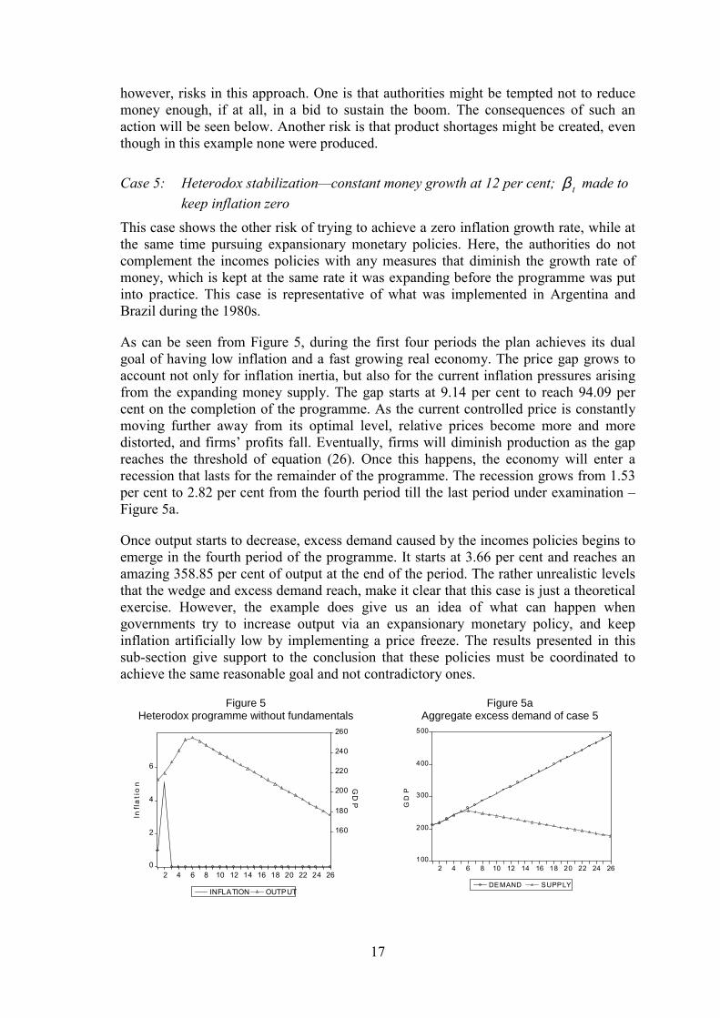
This case shows the other risk of trying to achieve a zero inflation growth rate, while atthe same time pursuing expansionary monetary policies. Here, the authorities do notcomplement the incomes policies with any measures that diminish the growth rate ofmoney, which is kept at the same rate it was expanding before the programme was putinto practice. This case is representative of what was implemented in Argentina andBrazil during the 1980s.

As can be seen from Figure 5, during the first four periods the plan achieves its dualgoal of having low inflation and a fast growing real economy. The price gap grows toaccount not only for inflation inertia, but also for the current inflation pressures arisingfrom the expanding money supply. The gap starts at 9.14 per cent to reach 94.09 percent on the completion of the programme. As the current controlled price is constantlymoving further away from its optimal level, relative prices become more and moredistorted, and firms’ profits fall. Eventually, firms will diminish production as the gapreaches the threshold of equation (26). Once this happens, the economy will enter arecession that lasts for the remainder of the programme. The recession grows from 1.53per cent to 2.82 per cent from the fourth period till the last period under examination –Figure 5a.

Once output starts to decrease, excess demand caused by the incomes policies begins toemerge in the fourth period of the programme. It starts at 3.66 per cent and reaches anamazing 358.85 per cent of output at the end of the period. The rather unrealistic levelsthat the wedge and excess demand reach, make it clear that this case is just a theoreticalexercise. However, the example does give us an idea of what can happen whengovernments try to increase output via an expansionary monetary policy, and keepinflation artificially low by implementing a price freeze. The results presented in thissub-section give support to the conclusion that these policies must be coordinated toachieve the same reasonable goal and not contradictory ones.

Figure 5Heterodox programme without fundamentals

Figure 5aAggregate excess demand of case 5

0

2

4

6

160

180

200

220

240

260

2 4 6 8 10 12 14 16 18 20 22 24 26

INFLATION OUTPUT

GDP

Inflation

100

200

300

400

500

2 4 6 8 10 12 14 16 18 20 22 24 26

DEMAND SUPPLY

GDP

18

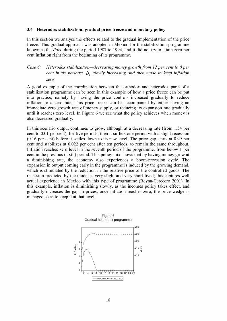
3.4 Heterodox stabilization: gradual price freeze and monetary policy

In this section we analyse the effects related to the gradual implementation of the pricefreeze. This gradual approach was adopted in Mexico for the stabilization programmeknown as the Pact, during the period 1987 to 1994, and it did not try to attain zero percent inflation right from the beginning of its programme.

Case 6: Heterodox stabilization—decreasing money growth from 12 per cent to 0 percent in six periods; β t slowly increasing and then made to keep inflationzero

A good example of the coordination between the orthodox and heterodox parts of astabilization programme can be seen in this example of how a price freeze can be putinto practice, namely by having the price controls increased gradually to reduceinflation to a zero rate. This price freeze can be accompanied by either having animmediate zero growth rate of money supply, or reducing its expansion rate graduallyuntil it reaches zero level. In Figure 6 we see what the policy achieves when money isalso decreased gradually.

In this scenario output continues to grow, although at a decreasing rate (from 1.54 percent to 0.01 per cent), for five periods; then it suffers one period with a slight recession(0.16 per cent) before it settles down to its new level. The price gap starts at 0.99 percent and stabilizes at 6.022 per cent after ten periods, to remain the same throughout.Inflation reaches zero level in the seventh period of the programme, from below 1 percent in the previous (sixth) period. This policy mix shows that by having money grow ata diminishing rate, the economy also experiences a boom-recession cycle. Theexpansion in output coming early in the programme is induced by the growing demand,which is stimulated by the reduction in the relative price of the controlled goods. Therecession predicted by the model is very slight and very short-lived; this captures wellactual experience in Mexico with this type of programme (Reyna-Cerecero 2001). Inthis example, inflation is diminishing slowly, as the incomes policy takes effect, andgradually increases the gap in prices; once inflation reaches zero, the price wedge ismanaged so as to keep it at that level.

Figure 6Gradual heterodox programme

0

2

4

6

8

210

215

220

225

230

2 4 6 8 10 12 14 16 18 20 22 24 26

INFLATION OUTPUT

GDP

Inflation

19

Even though output does experience a small recession once money growth is zero whileinflation is still positive, this policy does not cause excess demand because the gap inprices does not reach the levels required to achieve it. The size of the gap in prices of6.022 per cent, though not insignificant, is much less than under the shock programmeof achieving zero inflation right from the beginning of the programme (22.18 per cent).This difference in the size of the price wedge reflects what has already been stated: theprice gap depends on the magnitude of the diminished inertial component and presentdeterminants of inflation. Gradually increasing the gap offsets the inertial aspect ofinflation and the slow reduction of money growth reduces present inflation, thus makinga huge gap unnecessary. This combination also increases output indirectly bystimulating demand via changing relative prices, and directly by continuing to havepositive money growth for some time.

4 Concluding remarks

In this paper we developed a model which deals with the potential success of pricecontrols in stabilizing high inflation rates and their effects on the real economy under animperfect competition setting derived by optimal maximization. Our model builds onHelpman’s (1988) work on price controls and imperfect competition and incorporatesinflation inertia through adaptive expectations.

A central conclusion that seems to emerge from the previous analysis is that heterodoxprogrammes which only concentrate on the ‘hetero’ part of the effort, without attentionto the fundamental determinants of inflation, will be finally associated with adeteriorating performance on the output and inflation stabilization fronts. Enactingpolicies that pursue two different and conflicting goals, will fail to achieve either ofthem. The model presented here enables experiments to be carried out to analyse whichpolicy mix is more effective in bringing inflation down and what their respective costswill be in terms of output loss. Our model shows another path for the stabilizationbusiness cycle to take, without having to resort to exchange rate or credibility factors.The only factor needed is the effect of the price control upon the decisions of firms toaccommodate demand or not. Since all equations but one in the model are derived fromrational microeconomic behaviour, these decisions are always profit maximizing, and inline with the conventional wisdom on how firms operate.

A heterodox programme can be implemented following several and distinct policymixes, all with different outcomes. The policy of achieving zero inflation right away,with an accompanying shock treatment of monetary policy will eliminate inflation, butat the cost of a recession. The same policy with a gradual decline of money growth willachieve a boom followed by a slight recession. The major disadvantage of thisprogramme comes in the form of shortages in the economy, which will upset consumersand businessmen, and thus put extra pressure on the government to eliminate thecontrols. This is related to the greatest possible danger inherent in this type of policy,namely policymakers not actually lowering the rate of money growth. In casepolicymakers adopt the view ‘one more period of growth and then we can act’ on theassumption that this will not harm the economy, they are seriously mistaken. Thisbehaviour will distort relative prices beyond the limits tolerated by the private sector,which in turn will lower output; the final result will be that the more the governmentadds fuel to the economy, the deeper the recession becomes.

20

Any government instituting a stabilization programme will be burdened from the startwith credibility problems regarding policy management skills of the relevantgovernment authorities, the duration of the programme and, most importantly, theiractual intentions and goals. Bearing this in mind, even the most favourable heterodoxpolicy mix examined here, the gradual lowering of money growth and the phasedincrease in the intensity of the price freeze, can cause problems in achieving the goals.However, the shock treatment of money and the complete price freeze will successfullyachieve low inflation, but at the price of zero growth. Nevertheless, this result ispreferable to recession with inflation caused by an orthodox stabilization programme.Therefore, it is highly recommended for the government to gain credibility before theheterodox programme is implemented. Our simulation results are confirmed by thesensitivity analysis we conducted,11 although econometric analysis should beundertaken in future work, by using real data series on individual country basis, so thatmore robust results can be derived and policy lessons are learnt.

11 Sensitivity analysis results are available from the authors upon request.

21

Appendix

Helpman (1988) basically states that what a price control does is to set the control pricebelow what the optimal free price would be. This means that the controlled price can beexpressed as the optimal price divided by a variable that is greater than one:

(A.1)BP

Pt

jtjt

*

= 1≥Bt

where P jt is the government controlled price, P jt* represents the optimal

profit-maximizing price, and Bt stands for the wedge between the governmentcontrolled and optimal prices. In logs:

(A.2) β tjtjt pp −= *

where Btt log=β . This is equation (5) in the text. The advantage of representing a pricecontrol in this manner is that this equation is able to model the behaviour of the incomespolicy through time. Table 2 below shows the three possible paths β t can take:

Table 2Possible paths of price gap

Case 1 t-1 t t+1

Optimal price 5 8 10

Controlled price - 5 5

Gap - 37.50% 50%

Case 2 t-1 t t+1

Optimal price 5 8 10

Controlled price - 5 6.25

Gap - 37.50% 37.50%

Case 3 t-1 t t+1

Optimal price 5 8 10

Controlled price - 5 8

Gap - 37.50% 20%

Notes: Case 1: Constant controlled price and an increasing gap

Case 2: Increasing controlled price and a constant gap

Case 3: Increasing controlled price and a decreasing gap

In all cases periods 1−t and t are the same; at time 1−t there was no price freeze andthe optimal firm determined price is 5, at time t the government institutes a pricefreeze, setting prices for period t equal to prices at time 1−t . However, due to inertiaor some other factors the optimal price is now 8; thus, there the wedge is formed. Case 1illustrates the case where the government continues to set the same price at period 1+tas it did in period t , the optimal price has increased and so has the wedge. In case 2 thegovernment allows some adjustment of the controlled price to keep the wedge constant.

22

Finally, in case 3 the government has adjusted the controlled price to diminish thewedge; this could be the case where the government is slowly lifting the controls.Incorporating this pathway into the price freeze will give the model a possibility tomodel heterodox programmes in a dynamic manner which reflects the changes in theprogramme as circumstances change and new policy goals evolve.

23

References

Agénor, Pierre-Richard (1995). ‘Credibility of Price Controls in Disinflation Programs’.Journal of Macroeconomics, 17, (1): 161-71.

Agénor, Pierre, and Peter Montiel (1996). Development Macroeconomics. Princeton,NJ: Princeton University Press.

Aspe, Pedro (1993). Economic Transformation: The Mexican Way. Cambridge, MA:MIT Press.

Blanchard, Oliver, and Nobuhiro Kiyotaki (1987). ‘Monopolistic Competition and theEffects of Aggregate Demand’. American Economic Review, 77 (September):647-66.

Bruno, Michael, and Stanley Fischer (1990). ‘Seigniorage, Operating Rules, and theHigh Inflation Trap’. Quarterly Journal of Economics, May: 353-74.

Buira, Ariel (1983). ‘IMF Financial Programs and Conditionality’. Journal ofDevelopment Economics, 12: 11-136.

Calvo, Guillermo, and Carlos Végh (1994). ‘Credibility and the Dynamics ofStabilization Policy: A Basic Framework’, in Christopher Sims (ed.), Advances inEconometrics, Sixth World Congress, Vol. II. Cambridge: Cambridge UniversityPress.

Dertouzos, James N., and John H. Pencavel (1981). ‘Wage End EmploymentDetermination under Trade Unionism: The International Typographical Union’.Journal of Political Economy, 89 (6): 1162-81.

Dornbusch, Rudiger; Federico Sturzenegger, and Holger Wolf (1990). ‘ExtremeInflation: Dynamics and Stabilization’. Brookings Papers on Economic Activity, 1-84.

Helpman, Elhanan (1988). ‘Macroeconomic Effects of Price Controls: The Role ofMarket Structure’. The Economic Journal, 98 (June): 340-54.

Jensen, Henrik (1993). ‘Uncertainty in Interdependent Economies with MonopolyUnions’. Journal of Macroeconomics, 15 (1): 1-24.

Naish, Howard F. (1988). ‘Optimal Union Wage Setting Behaviour and the Non-neutrality of Anticipated Monetary Changes’. Oxford Economic Papers, 40: 346-64.

Oswald, Andrew J. (1982). ‘The Microeconomic Theory of the Trade Union’. TheEconomic Journal, 92 (September): 576-95.

Rebelo, Sergio, and Carlos Végh (1995). ‘Real Effects of Exchange Rate-basedStabilization: An Analysis of Competing Theories’, in Ben Bernanke and JulioRotemberg (eds), NBER Macroeconomics Annual. Cambridge, MA: MIT Press.

Reyna-Cerecero, Mario A. (2001). ‘Orthodox and Heterodox Stabilization Programs:Theory and Policy’. Manchester: University of Manchester. Ph.D. Thesis.

Roldós, Jorge E., (1995). ‘Supply-side Effects of Disinflation Programs’. IMF StaffPapers, 42: 158-83.

van Wijnbergen, Sweder (1988). ‘Monopolistic Competition, Credibility and the OutputCosts of Disinflation Programs: An Analysis of Price Controls’. Journal ofDevelopment Economics, 29: 375-98.