PROCEEDINGS, Thirty-Fifth Workshop on Geothermal Reservoir Engineering Stanford University, Stanford, California, February 1-3, 2010 SGP-TR-188

INFLUENCE OF GEOLOGICAL STRUCTURES ON FLUID AND HEAT FLOW FIELDS

J. Florian Wellmann, Franklin G. Horowitz, Klaus Regenauer-Lieb

Western Australian Geothermal Centre of Excellence (WAGCoE) The University of Western Australia

Crawley, WA, 6100, Australia E-mail: wellmann@cyllene.uwa.edu.au

ABSTRACT

Geothermal exploration is commonly performed in the absence of 3-D seismics or other high quality methods constraining the geometry of the underlying geological system. Therefore, uncertainty resides in the structural model itself. This is in addition to the usual assumption of stochasticity in the petrophysical properties. We show here that small changes in the geometrical description of the geology can produce large changes in the character of heat transport. Combining these sensitivities with the inherent uncertainties in geological model characterization, we suggest that the careful consideration of the systematics of geothermal heat transport is warranted. At present, these sensitivities are not widely recognized because the infrastructure to explore these links has not previously existed to the best of our knowledge. We have therefore constructed an integrated workflow that combines geological modeling directly with fluid and heat flow simulation. This allows us to calculate the heat transport variability in an ensemble approach. We apply our method to a geological model of the North Perth sedimentary basin in Western Australia. For interpretation of the results, we suggest a particularly useful analysis is the spatial variability of temperature fluctuations combined with the variability of the Peclet numbers in horizontal and vertical directions.

INTRODUCTION

Geothermal simulation is an essential part of exploration and reservoir utilization (e.g. O’Sullivan, 2001). However, a model can never be a perfect representation of the real world and uncertainties and misfits remain. The sensitivity of a model with respect to the physical properties is commonly evaluated, but the effect of uncertainties in the underlying geological structure model is rarely considered.

We hypothesize that uncertainties in the structural model have a significant influence on the simulated fluid and heat flow fields. To test this hypothesis, we develop an integrated workflow that links geological raw data with the flow simulation. This enables testing the sensitivity of the flow fields to changes in the geological model. It also opens the way to geological data-driven geothermal inversion. In this paper, we evaluate some simple examples of how the subsurface structure influences the single-phase flow field by studying the onset of convection in a hot sedimentary aquifer. We then present some fundamental uncertainties present in geological models. Next, we explain our method of an integrated workflow for geological modeling and geothermal simulation. We then show how to use this workflow to evaluate the effect of uncertainties in the geological model on the flow field. We give an example of how the approach can be applied to realistic scenarios and how the results can be interpreted. Finally, we discuss further possibilities and future work to extend the approach.

INFLUENCE OF SUBSURFACE STRUCTURE ON FLUID FLOW

We demonstrate one important example of how the subsurface structure influences fluid flow by considering the onset of convection in a porous medium.

Theoretical considerations A non-linear effect is present if small changes in some properties lead to a significant change in the model. One of the best known and most important non-linear effects in fluid and heat flow is the onset of free convection. The Rayleigh number (Ra) determines the system state with respect to fluid properties, permeability, thermal conductivity and geothermal gradient. For porous media and a 2-D layer heated from below, it is defined as

m

pff TTkbcgRa

µλρα )0

2 ( −≡

where α f is the coefficient of thermal expansion, g is

the acceleration of gravity, ρ f is fluid density, cp is heat capacity, k is permeability, b is layer thickness, T is the temperature at bottom of the layer, T0 is the temperature at the top of the layer, µ is the viscosity, and λm is thermal conductivity. The fluid starts to convect once this number reaches a threshold value, the critical Rayleigh number ( Racrit = 4π 2 for the assumption that only density changes with temperature are considered). This changes the character of the fluid and heat flow fields completely. From the definition of the Rayleigh number, we can see its direct dependence on permeability k and temperature difference (T-T0). These parameters are commonly tested in sensitivity analyses for the flow field. Permeability is especially important as it can vary by several orders of magnitude for different rock types. We show here another important sensitivity, namely the dependence on the thickness of the formation (b).

Example simulation Consider a very simple double layered model (Fig. 1, upper part) with a permeable layer bounded by an impermeable layer above. For conditions below the critical Rayleigh number, we find a nearly linear temperature pattern (Fig. 1, Model 1: Temperature). If we increase the thickness of the permeable layer by

10 meters (Fig. 1, Model 2: Geology), the temperature field does not change significantly (Model 2: Temperature). But if we increase the layer thickness by another 10 meters (Fig. 1, Model 3: Geology) the system rises above the critical Rayleigh number, and convection begins. We obtain a completely different fluid and heat flow pattern (Model 3: Temperature). This is a (Hopf) bifurcation from a conductive to a convective system; in this case only due to the increased thickness of the permeable layer, all other parameters being constant. This is just an illustrative example to demonstrate how changes in the subsurface structure affect the fluid and heat flow fields. But it suggests the importance of considering uncertainties in the underlying geological model since the character of the solution changes dramatically with a 1% change in thickness.

UNCERTAINTIES IN GEOLOGICAL MODELS

For the purpose of this paper, we define geological models as structural representations of the subsurface derived from the interpolation of a variety of data sources like seismic reflection data, well-logs or field observations and measurements. Uncertainties in these geological models occur for a variety of different reasons (Fig. 2). The first type of uncertainty (Fig. 2a) is directly related to the quality of the data that are used for modeling. Geological observations usually contain a degree of uncertainty, especially if they are indirectly interpreted, e.g. from well-logs. This adds a significant degree of uncertainty to the structural model.

Figure 1: Non-linear effect of formation thickness change on the temperature pattern. Model 1: simple geological model with a permeable formation (7*10-13m2) overlain by an impermeable layer. The simulated temperature field is mainly linear with some minor instability. Model 2: the permeable layer is increased by 10m, the temperature field is similar to the first Model. Model 3: thickness of permeable layer increased by another 10m: the character of the simulated temperature field changes completely due to the onset of convection. Only formation thickness is changed, all other parameters are the same as before.

Figure 2: Different types of uncertainties typically

encountered in structural geological modelling

The next problem is related to the quality of the interpolation applied between data points (Fig. 2b). Many tools can be used to interpolate, ranging from simple Bezier methods to complex geostatistical interpolations (e.g. Mallet, 1992; Lajaunie, 1997). All have different advantages and disadvantages, but there always remains an uncertainty of the interpolation quality between observation points. Finally, even for the best interpolation and high-quality data points, we never know if our knowledge about the relevant structures in the subsurface is complete (Fig. 2c). In a recently submitted paper (Wellmann, submitted) we propose that model uncertainties derived from inaccuracies in the raw data (Fig. 2a) can have a significant influence on the modeled subsurface structure. We developed a method similar to conditional simulation that generates uncertainties in the results. Each model respects the probability distributions and structural dependencies for boundary observations and orientation measurements. Figure 3 shows an example model where multiple simulated formation surfaces are plotted into the same section.

Figure 3: Result of uncertainty simulation for a

simple model with formations in a graben setting. The lines represent the top surface of a formation. All modeled surfaces for several simulated input data sets are plotted into one section, different colors represent different formations.

We can use the simulated models for statistical analyses and e.g. calculate the mean surface and standard deviation maps (Figure 5). This provides a further insight into areas of high and low certainty within the model.

Figure 4: Statistical analysis of all simulated

surfaces of one formation (red formation in Fig. 4): map of standard deviations projected on mean surface. We can clearly identify areas of high uncertainty around the faults.

While this approach works well for 2.5-D like settings (only one point for each formation at every location), it gets more complicated if we consider a full 3-D setting, for example with reverse faulting or dome structures. To treat these more complex settings, we developed an approach that is applicable to many types of possible structures based on indicator functions. The indicator function of a formation F is a subset of the whole model space defined as

⎩⎨⎧

∉∈

=Fx

FxxIF for 0

for 1)(

For a practical application, we can apply this formulation to a discretized version of the model (e.g.

a regular mesh) and thus derive a mesh with cell values 0 or 1 for each formation in a model. It is now straight-forward to calculate the minimal and maximal extent of a formation F for n simulated models as

∏∈

=nk

FF kII

min

)1(1max ∏

∈

−−=nk

FF kII

Figure 5 shows an example of a complex dome setting with calculated minimal extent (red surface) and maximal extent (blue transparent surface) of all simulated models.

Figure 5: Minimal and maximal extent of all

simulated models for a dome structure calculated with the indicator formulation described above. The “Indicator sum” (color bar) is another way to display the model variations showing isolines for the extent of a certain number of models

For further details about the uncertainty simulation itself and the parameters and probability distributions applied to the example models, please see Wellmann (submitted). For the work presented in this paper, we consider as important to point out that structural models can contain significant uncertainties and that ways to display and analyze these uncertainties exist. Combining this finding with the realization that already small changes in the structural model can have a significant influence on the flow field (see above), we attempt to develop tools to evaluate this effect in simulated models by combining both steps, uncertainty evaluation of the structural model and subsequent fluid and heat flow simulation, into one combined, integrated workflow.

COUPLING GEOLOGICAL MODELING DIRECTLY TO FLUID FLOW SIMULATION

Standard approach and relevant steps Before we describe our approach of an integrated workflow, we want to briefly outline the standard steps to compute a fluid and heat flow model for a geothermal resource area

Geological model The first step is usually to create a structural representation of the subsurface, a geological model, as a starting point for the fluid and heat flow simulation. This can range from very simple plate models to highly complex interpolations of a variety of input data in full 3-D. Many different (mostly commercial) tools exist to create subsurface models (e.g. Calcagno, 2008; Turner, 2006; Mallet, 1992), mainly differing in the way they interpolate between data points (e.g. surface or volume methods) and the flexibility of input data types they can deal with (seismics, well-logs, structural measurements, etc.). All these approaches have different advantages and disadvantages but finally the aim to create a representation of the subsurface structure that can be combined to fluid and heat flow properties for the simulation. In this sense, the scale of the subsurface model has to be chosen to reflect the details that are relevant for the scale of the simulation.

Processing of the subsurface model to a simulation grid The structural model has to be discretized into a format that is recognized by the simulation code. Typical examples are rectilinear meshes for finite difference (FD) simulation codes or tetrahedral meshes for finite element (FE) codes, but many other mesh types are possible. Depending on the complexity of the structural model, and the required mesh discretization, this step can be very tedious and time-consuming.

Fluid and heat flow simulation After the subsurface model is discretized into a mesh format, fluid and heat flow properties can be assigned to the different structural domains. The used properties depend on the type of simulation, typically for single phase fluid and heat flow simulations at least permeability, porosity, thermal conductivity and heat production rate are required. The next step is then to assign boundary conditions for the simulation, where typical conditions are fixed head/ temperature, constant flux or no flow. A variety of different software codes exists for the geothermal simulation itself (see e.g. O’Sullivan, 2001, for an overview and also a discussion about typical boundary conditions).

Processing and analysis of results After simulation, a variety of possibilities exists for further processing of the results. Many post-processing tools allow a visualization of the results (mainly fluid pressure and temperature field) in 3-D. Depending on the nature of the study, it might also be interesting to analyze specific features of the model in more detail. In the case of geothermal exploration for hot sedimentary aquifers, it is, for example, specifically interesting to determine areas with high temperatures and hydraulic conductivities to obtain optimal pumping rates.

Integration into one workflow and linking of single steps Most of the steps described above require at least some manual work, depending on the complexity of the structural model and the type of discretization. Thus, if the initial structural geological model is changed, e.g. for scenario testing, it can be tedious and time-consuming to update the results of the flow simulation. In order to evaluate the effect of uncertainties in the structural model on the flow field, it is necessary to reduce these manual steps to a minimum. We therefore designed an integrated workflow that combines the steps described. We used the following techniques to achieve this (see Table 1 for a summary):

Geological Modelling We apply the potential-field approach for the geological modelling that is used in the software GeoModeller (for detailed information see www.geomodeller.com and Calcagno, 2008). This modelling technique allows the direct update of the geological model when the input data are changed or new data are added.

Meshing We implemented automated mesh generation algorithms that create rectilinear meshes from the geological model. These can be used for finite differences/ finite volume flow simulation codes (e.g. SHEMAT, see Clauser, 2003 and/or TOUGH2, see Pruess, 1991).

Simulation update The input file for the simulation is updated directly based in the changed geological model. All parameters that are linked to a geological structure are adapted, all others remain constant (e.g. boundary conditions, convergence criteria, etc.).

Combining uncertainty simulation of geological model directly with flow simulation We can now combine the integrated workflow with the uncertainty simulation of the structural model. Instead of only processing one geological model to the fluid and heat flow simulation, we process several structural representations simultaneously (Figure 6). As the single steps of the workflow are automated, no further manual steps are required here. Thus, we obtain several simulated fluid and heat flow fields. The differences are solely due to changes in the initial structural model, all other parameters are kept constant in this analysis to detect the influence of the structural uncertainty.

Figure 6: Flow chart for the combination of

structural uncertainty simulation with the integrated workflow from meshing to flow simulation: instead of processing only one structural model and calculating its flow fields, several structural representations are processed simultaneously

Table 1: Overview of the common process steps from geological data points to simulated fluid and heat flow fields; In the column “Automation”, our steps to link the different parts into one integrated workflow are summarizes

Process Description Automation

Raw data discretization Digitalization of observed or inferred data points and observation measurements into a modeling framework; Changing and adjusting existing points and observations

Use of xml file format to store data (GeoModeller format); possible to access and change data with own scripts (e.g. for random changes in uncertainty simulation)

Geological modeling Interpolation of observed or interpreted data points in a model domain respecting geological reasoning (stratigraphy, faulting, etc.)

Using GeoModeller as modeling software: enables direct model update when input data are changed; external control of software with own scripts

Mesh generation Discretization of geological model into a mesh format that can be used with simulation code (i.e. suitable for Finite Element, Finite Difference, Finite Volume, etc. calculations)

Rectilinear mesh generation with export function in GeoModeller and own scripts

Set-up of simulation Import discretized model into a format useable by simulation code; assign fluid and thermal properties to cells; definition of model parameters (e.g. convergence criteria, time steps) and boundary conditions

Automated update of a pre-defined template file with own scripts

Fluid and heat flow simulation Coupled fluid and heat flow simulation; visualization, processing and analysis of results

Simulation with TOUGH2 and/or SHEMAT; post-processing and data analysis with own scripts

50403020

EXAMPLE SIMULATION NORTH PERTH BASIN

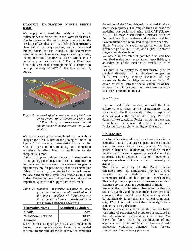
We apply our sensitivity analysis to a hot sedimentary aquifer setting in the North Perth Basin. The formation of the Perth Basin is related to the break-up of Gondwana. It is a half-graben structure, characterized by deep-reaching normal faults and internal horsts (see Fig. 7 and 8). The sedimentary basin is several kilometers deep containing clastic, mainly terrestrial, sediments. These sediments are partly very permeable (up to 1 Darcy). Basal heat flux in the area of this example model is assumed to be approximately 80 mW/m2 (Hot Dry Rocks Ltd, 2009).

Figure 7: 3-D geological model of a part of the North

Perth Basin; Model dimensions are 50km x 50km * 8km; the cross-section and all simulations are based around the yellow section.

We are presenting an example of our sensitivity analysis for a 2-D subset of the geological model in Figure 7 for convenient presentation of the results. Still, all parts of the modeling and simulation workflow described here are applicable to the complete 3-D model. The box in figure 8 shows the approximate position of the geological model. Note that the drillholes do not penetrate the basement. We therefore assigned a high uncertainty for positioning of the basement (see Table 2). Similarly, uncertainties for the thickness of the lower sedimentary layers are affected by this lack of data. We furthermore assigned an uncertainty to an important aquitard in the upper part of the model. Table 2: Statistical properties assigned to three

formations in the model; Positioning of the lower interface of formations are drawn from a Gaussian distribution with the specified standard deviations.

Formation Name Standard deviation Cadda 20m Woodada-Kockatea 100m Permian 200m

Based on these assigned properties, we simulated 20 random model representations. Using the automated software framework described above, we combined

the results of the 20 models using assigned fluid and heat flow properties. The coupled fluid and heat flow modeling was performed using SHEMAT (Clauser, 2003). The mesh discretization, interface with the fluid and heat flow database and the fluid and heat flow simulation are automated using Python scripts. Figure 9 shows the spatial resolution of the finite difference grid (25m x 100m) and Figure 10 shows a single example simulation. We obtain an ensemble of possible fluid and heat flow field realizations. Statistics on these fields give an indication of the locations of variability in the results. In Figure 11, we display the spatial variability of the standard deviation for all simulated temperature fields. We clearly identify locations of high uncertainty in the resulting temperature fields. To obtain an insight into the spatial variability of heat transport by fluid or conduction, we make use of the local Peclet number defined as Pe = l * v / κ For our local Peclet number, we used the finite difference grid sizes as the characteristic length scales l, v is the fluid velocity in the corresponding direction and κ the thermal diffusivity. With this definition, we calculated Peclet numbers in the x- and z-directions. The standard deviations of the local Peclet numbers are shown in Figure 12 a and b.

DISCUSSION

Our hypothesis is confirmed: small variations in the geological model have large impact on the fluid and heat flow properties of these systems. We have presented here a methodology to assess these impacts for the specific case of sparse geological control on structure. This is a common situation in geothermal exploration where 3-D seismic data is normally not available. The spatial variability of the Peclet number calculated from the simulations provides a good indicator for the reliability of the predicted temperature fields and heat transport mechanisms. This is of primary importance for assessing models of heat transport in locating a geothermal drillhole. We note that an interesting observation is that the spatial variability and the magnitude of the horizontal component (Fig. 12a) of the Peclet number appears to be significantly larger than the vertical component (Fig. 12b). This could affect the risk analysis for a geothermal siting decision. This approach complements the standard stochastic variability of petrophysical properties as practiced in the petroleum and geostatistical communities. We leave for future work the combination of our approach with these traditional methods and with multiscale variability obtained from forward simulations of sedimentary processes.

Figure 8: Cross-section of the North Perth Basin (Mory, 1996) showing the boundary fault in the East (Darling Fault) and the internal horst-graben structures with deep-reaching normal faults cutting into the basement (pink). The oldest sedimentary formation is Permian (light blue), the youngest in this part of the basin Jurassic (light green). The grey box shows the position of the simulated example sections.

Figure 9: Discretized model: regular mesh with a cellsize of 200m x 25m; the inset shows the resolution of the thin layers

Figure 10: Temperature distribution in one of the simulated models

Figure 11: Spatial variability of the standard deviation for all simulated temperature fields; we can identify areas in the model that are particularly sensitive to uncertainties in the geological model in the lowest layer and areas that are relatively stable; the lines show one geological model representation

ACHKNOWLEDGEMENT

J. Florian Wellmann is supported by an International Postgraduate Research Scholarship (IPRS) from the Australian Government and an Ad-hoc Scholarship by Green Rock Ltd. Conference attendance is made possible by a UWA Graduate Research Student Travel Award. The Western Australian Geothermal Centre of Excellence (WAGCoE) is a joint center between Curtin, UWA, CSIRO and funded by the Western Australian State Government.

REFERENCES

Calcagno, Ph.; Chilès, J-P.; Courrioux, G.; Guillen, A. (2008): Geological modelling from field data and geological knowledge: Part I. Modelling method coupling 3D potential-field interpolation and geological rules. Physics of the Earth and Planetary Interiors, 171

Clauser, Ch; Bartels, J (2003): Numerical simulation of reactive flow in hot aquifers. SHEMAT and processing SHEMAT. Berlin: Springer.

Hot Dry Rocks Ltd (2009): Geothermal Energy Potential in Selected Areas of Western Australia (Perth Basin). A report prepared for the Department of Industry and Resources, Western Australia. Department of Mines and Petroleum. Government of Western Australia.

Lajaunie, C.; Courrioux, G.; Manuel, L. (1997): Foliation fields and 3D cartography in geology: Principles of a method based on potential interpolation. Mathematical Geology, 29, 571–584.

Mallet, J-L. (1992): Discrete smooth interpolation in geometric modelling. Computer-Aided Design, 24, 178–191.

Mory, A. J., and Iasky, R. P. (1996): Stratigraphy and structure of the onshore northern Perth Basin, Western Australia: Western Australia Geological Survey, Report 46.

O'Sullivan, M. J.; Pruess, K.; Lippmann, M. J. (2001): State of the art of geothermal reservoir simulation. Geothermics, 30, 395–429.

Pruess, K. (1991): TOUGH2: A general-purpose numerical simulator for multiphase fluid and heat flow. Lawrence Berkeley Lab., CA (United States). (Technical Report).

Turner, A. (2006): Challenges and trends for geological modelling and visualisation. Bulletin of Engineering Geology and the Environment, 65, 109–127.

Wellmann, J. F.; Horowitz, F. G.; Schill, E.; Regenauer-Lieb, K. (submitted): Uncertainty simulation improves understanding of 3-D geological models. Submitted to Tectonophysics

(a)

(b)

Figure 12: Spatial variability of standard deviation of the calculated Peclet numbers in x-direction (a) and z-direction (b); With this analysis, areas in the model are highlighted where fluid velocities are changing significantly; As the fluid driver is free convection in this case, we can identify areas where the position of convection cells is sensitive to uncertainties in the geological model. This is relevant for geothermal exploration in hot sedimentary aquifers where upwelling zones of convection cells are a favourable target.