ABSTRACT The objective of the present work is to investigate the effect of the Earth’s oblateness
parameters, particularly J2, on the formation flight of micro satellites in low circular orbits. For this purpose, the Clohessy-Wiltshire equations, which have been accordingly modified, will be reviewed to arrive at a convenient formulation as a set of linearized differential equations of motion to include the J2 effects in the LVLH frame of reference. Comparison will then be made between the orbit of twin-satellite formation flying with respect to that predicted by the Hill-Clohessy-Wiltshire equation. Results obtained compare well with those in the literature and can be utilized for further development, parametric studies and mission design. Keywords: Orbital Mechanics; Gravitational Potential; Spacecraft Formation Flying.
INTRODUCTION
The interest in using multiple spacecraft for interferometry, space-based communications, and missions to study the magnetosphere prompted studies on the relative motion dynamics and control of spacecraft in formation flight. Specific insight into formation geometry is needed for mission planning and reconfiguration, which is not be possible without accurate description of the dynamics and optimal control methods. A closed path of relative motion traced out by a spacecraft under force-free motion as stipulated by Yeh and Sparks (2000), satisfying the Hill-Clohessy-Wiltshire (HCW) equations, must lie on the intersection of a plane and an elliptic cylinder with an eccentricity of 3/2 in a moving coordinate system fixed to the chief spacecraft in the Local-Vertical-Local Horizon (LVLH) frame of reference. The plane can be at any slope that is not perpendicular to the orbit plane of the chief satellite, as the elliptical cylinder lies normal to the orbit plane. In the well-known HCW equation, the Earth is regarded as a point mass. However, it is also well known that the Earth’s gravitational potential can also be represented by a spheroid (Vinti, 1971) or other harmonics (Alfriend, Gim, & Schaub, 2000). By linearizing the gravitational terms in the presence of J2 , the Earth’s dominant oblateness parameter, for the deputy satellite with respect to the chief’s reference orbit, analytical solutions similar to that of the HCW equations are obtained. These J2 -Modified Hill’s Equations describe the mean motion changes in both the in-plane and out-of-plane motion considerably well. The objective of the present work is thus to develop a computational routine and investigate the effect of the Earth’s dominant oblateness parameters, particularly J2, on the formation flight of micro satellites in low circular orbits for further applications.
Djojodihardjo /International Journal of Automotive and Mechanical Engineering 9 (2014) 1802-1819
1803
COORDINATE SYSTEM TRANSFORMATION
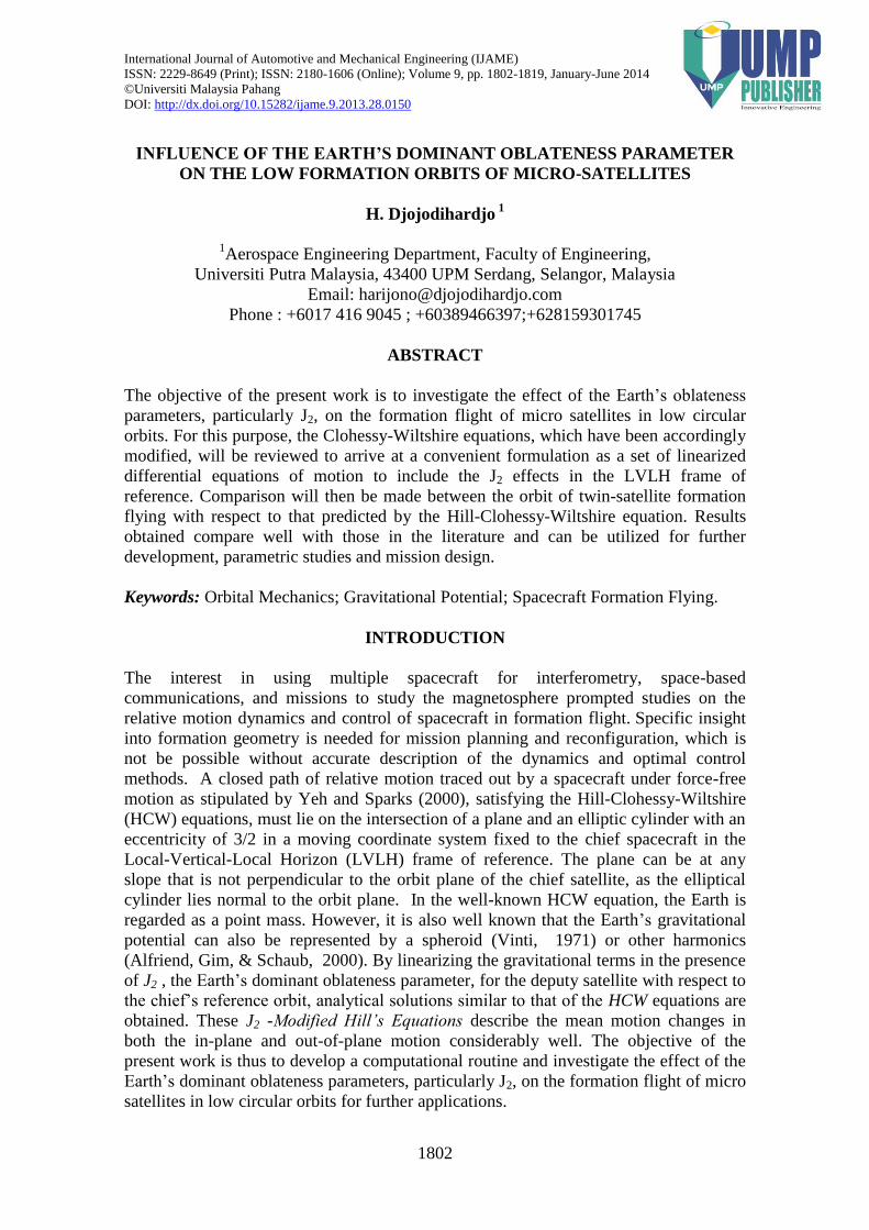
Referring to the coordinate system conventionally utilized as described by Alfriend et al. (2000), here the subscript N denotes a vector in the ECI frame, and a subscript O denotes a vector in the satellite-centered frame. The ( r −θ − i ) coordinate system (or Earth Centered Chief Satellite Orbital Plane coordinate system) is used to describe the J2 disturbance in the local ( x - y - z ) coordinate system. The presence of r and the two Euler angles, θ and i , completes the geometry of the associated transformation from the ECI frame to the ( r −θ − i ) frame, utilizing the direction cosine matrix formed by the 3-1-3 Euler angle sets Ω , i and θ . This is shown in Figure 1 and defined as the longitude of the ascending node, the argument of latitude, and the inclination angle, respectively.
cos cos sin sin cos sin cos cos sin cos sin sin
cos sin sin cos cos sin sin cos cos cos cos sin
sin sin cos sin cos
i i i
ON i i i
i i i
(1)
A similar direction cosine matrix (DCM) is written in terms of the LVLH
coordinate frame as described in the ECI frame, which is a direct rotation from the ECI coordinates into the satellite-centered frame. As such, these two rotations are equivalent.
rX rY rZ
X Y Z
hX hY hZ
e e e
ON e e e
e e e
(2)
Figure 1 depicts the various relevant coordinate systems used.
Figure 1. The ( r −θ − i ) coordinate system is used to describe the J2 disturbance in the local ( x - y - z ) coordinate system.
1804
FORMATION FLYING AND RENDEZVOUZ PROBLEM Spacecraft formation flying involves multiple spacecraft orbiting a common primary in close proximity. One of the spacecraft will be referred to as the chief and the others as the deputies. This terminology is used in a more general arrangement. Different terminologies such as leader-follower or target-chaser are also used depending on the nature of the formation structure. In a formation flight, there is usually only one chief satellite while there can be multiple numbers of deputies. The chief need not to be a physical spacecraft but can be modeled as a fictitious spacecraft acting as a reference point or a reference orbit for the spacecraft formation. Two spacecraft can be maneuvered in several ways. One spacecraft could already be in an orbit (referred to as the target) and the other could be in a different orbit (the chaser), or more generally a different position in space. The chaser, then, can perform an orbital transfer maneuver to achieve its determined objective, whether to achieve a similar orbit, to intercept the target or to follow the target in close proximity. In order to analyze this situation, one needs the positions and velocities of the two spacecraft to be known in a similar coordinate system. One can then define the position vectors and the velocity vectors of the target and chaser (LVLH frame). The deputy satellite position and velocity vector is
T
c c c ct x y zX (3a)
T
c c c ct x y zV (3b) We then define define the difference or relative position and velocity between the two spacecraft as
d ct X X X (4a)
d ct V V V (4b)
where subscript c refers to Chief (Target, Leader)-Satellite and d refers to Deputy (Chaser, Follower)-Satellite. This relative motion can be classified into several categories. The category is defined by the boundary conditions that need to be satisfied, associated with the mission. The terminal time, when the deputy satellite accomplishes the mission, will be denoted by tf. Rendezvous: For a space rendezvous, two spacecraft need to be in the same position on an orbital with the same velocities at the end of the maneuver, and no constraint imposed on the initial conditions of the two spacecraft. This requires six boundary conditions with every element in position and the velocity vectors the same at the end of the maneuver:
0d ct X X X (5a)
0d ct V V V (5b)
Djojodihardjo /International Journal of Automotive and Mechanical Engineering 9 (2014) 1802-1819
1805
Intercept: For the chaser to intercept the target only the position vectors of the two spacecraft need to be equal. This can be compared with a missile trying to hit a moving target, for instance. Only three boundary conditions are required.
0fx t ; 0fy t ; 0fz t (6)
Orbital transfer: In this case, the chaser does not need to “touch” the target, it is sufficient for it to be in the target’s orbit. To achieve this, five boundary conditions are
needed.
0fx t ; 0fz t ; 0fx t ; 0fy t ; 0fz t (7)
Stand-off rendezvous: In this type of rendezvous, the chaser does not “touch” the target, but rather remains in a close proximity in a bounded motion around the target. The distance between the chaser and the target is defined as the vector 𝝆.
ft X ρ ; 0ft V (8)
This type of rendezvous is fundamental for initializing spacecraft to fly in
formation (close proximity to each other). Ideally, in formation flying, one would like to maintain the position of the follower with respect to the leader at all times during a space mission (one may alternatively use the terminology follower-leader to better suit the nature of the problem). For the present work, it is sufficient that the followers be in proximity with the motion around the leader, or in other words, are “bounded”.
LINEAR MODEL OF RELATIVE DYNAMICS The objective of this section is to determine the equations of motion for the deputy spacecraft relative to the chief spacecraft. The following development closely follows that of Alfriend et al. (2000). Figure 2 shows two spacecraft in Earth orbit. The inertial position vector of the chief is R, and that of the deputy is r. The position vector of the deputy relative to the chief is ρ, such that
r R ρ or d cr r ρ (.9)
Figure 2. Coordinate System for defining relative motion.
1806
One of the assumptions that should be made at this stage is that the relative
distance between chief and deputy is small compared to the magnitude of R, e.g. 1R
.
Following Newton’s Gravitational Law, the equation of motion for an earth-orbiting body is:
3
; rr
r r r 3
; d d d dd
rr
r r r (10a)
as well as
3
; RR
R R R 3
; c c c cc
rr
r r r (10b)
Here is the standard gravitational constant of the earth, which is 3986km3/sec2. In what follows, all perturbation components (derived from the propulsive force, J-perturbation, aerodynamics drag or third-body forces) will be ignored in Eq. (10) at the present stage. The vectors are all t-dependent. The equation of motion for the deputy in the moving frame can be further elaborated by substituting Eq. (.9) (into Eq. (10) to obtain the equation of motion for the deputy satellite. Hence:
3
r R ρ R ρ
R ρ (11)
and, subsequently
3
ρ R R ρ
R ρ (12)
For circular orbit, 3
R represents the angular rate of the circular orbit
around the center of Earth in the orbital plane. Here R is the semi-major axis or radius of the circular orbit and ρ is the position vector of the deputy spacecraft in the relative (moving, orbiting) frame around the chief spacecraft. Accordingly:
3
0 00
0 0 ; ; ;0
Rx
y
zR
ω R ρ (13)
For the right-hand side of Eq. (12) , one can expand 3
R ρ in a Taylor series
approximation. Taylor series expansion about 3
0,F
R ρ R ρ yields
3 3
32 2
2 2 2 3 2 2
3 4 5 5 5 6 6 6
2
1 3 6 3 3 10 15 15...
2 2 2 2
x x y z x xy xz
R R R R R R R R
R ρ R ρ R ρ R R R ρ ρ ρ
(14)
Djojodihardjo /International Journal of Automotive and Mechanical Engineering 9 (2014) 1802-1819
1807
Substituting Eq.(14) into Eq. (12) one obtains
2 2 2 3 2 2
3 4 5 5 5 6 6 6
1 3 6 3 3 10 15 15..
2 2 2 2
x x y z x xy xz
R R R R R R R Rρ R R ρ (15)
Neglecting the terms with an order higher than one, Eq. (15) becomes
3 3 2
3
R R R
Rρ R ρ R ρ R (16)
Substituting the equation of motion for the chief satellite 3R
R R into
Eq. (16), one finally obtains:
3 2
3
R Rρ ρ R ρ R (17)
Eq. (17) yields the desired relationship for �̈� in the inertial frame I. One needs to
represent 𝝆 in the relative frame, R, around the chief spacecraft. One can write �̈�𝐼 in the inertial frame as:
2I R R R R ρ ρ ω ρ ω ω ρ ω ρ (18)
Thus, �̈� in the relative frame:
2R I R R R ρ ρ ω ρ ω ω ρ ω ρ (19)
Substituting Eq. (13) into Eq. (19) and keeping only the linear terms, one obtains the kinematic relationship:
2 22 2 x y x y x y zρ i j k (20)
Substituting Eq. (13) to Eq. (20) yields the equation of motion:
2
2
3
x y z R x R
Rρ i j k i (21)
Combining the kinematic relationship (17) with the equation of motion (21) yields:
2 22 3 2 0 x y x y x z zi j k (22)
Hence, Eq. (22) gives the linearized Clohessy-Wiltshire equation:
22 3 0 x y x (23a)
1808
2 0 y x (23b)
2 0 z z (23c)
This set of equations refers to the moving frame of reference in which they were derived. This moving frame is sometimes called CW-frame or Hill’s frame. One
advantage of the CW equations is that the in-plane orbital motion (x and y directions) is uncoupled from the out-of-plane orbital motion (𝛿𝑧 direction). In the present CW equations, the following assumptions are made:
i. The eccentricity of the chief orbit is zero (circular), e=0 ii. The angular rate is constant, �̇�=0 iii. 𝑅 is constant (circular orbit)
Next the homogeneous solution of the CW equations will be derived. Define
T
x y zX and T
x y zV . A subscript 0 denotes the initial
condition. The solution of the linearized CW equations can then be represented in the following matrix form:
0 0XX XVt X X V (24)
where,
4 3cos 0 0
6sin 6 1 0
0 0 cosXX
t
t t
t
;
sin / 2 1 cos 0
2 1 cos / 4sin / 3 0
0 0 sin /XX
t t
t t t
t
(25)
0 0VX VVt V X V (26)
where,
3 sin 0 0
6 1 cos 0 0
0 0 sinVX
t
t
t
: cos 2 1 cos 0
2sin 3 4cos 0
0 0 cosVV
t t
t t
t
(27)
Eq. (24)-(27) then describe the homogeneous solution of the Clohessy-Wiltshire (CW) equation, which determines the position of the deputy spacecraft relative to the chief spacecraft as a function of t subject to initial conditions X0 and V0.
BASELINE HILL-CLOHESSY-WILTSHIRE EQUATION: For a point mass or uniformly distributed sphere, the gravitational potential is
14 3 23.986005 10 /eGM m s (28)
which is the first term of the more general gravitational potential of the Earth. If J2 is included, we have (Alfriend et al., 2000; Djojodihardjo, 1972).
Djojodihardjo /International Journal of Automotive and Mechanical Engineering 9 (2014) 1802-1819
1809
2
223
3 1cos
2 2eR J
U
(29)
Baseline Hill-Clohessy Wiltshire Equations, for circular orbit around the Earth
as the central body, assumed the Earth as the point mass centered at its center of mass and the center of the orbit. The equations of motion in the chief LVLH frame:
2
22
2 3 0d x dy
xdtdt
(30a)
2
22 0
d y dxdtdt
(30b)
2
22
0d z
zdt
(30c)
are also known as the Unperturbed HCW Equations. The angular velocity is given by:
3 3
G M m
r r (31)
The out-of-plane motion is modeled as a harmonic oscillator, where the in-plane motion is described as a coupled harmonic oscillator. These second-order differential equations have the general solutions:
cos offx t A nt x
3
2 sin2 off offy t A nt nx t y (32)
cosz t B nt
where A, α, xoff , yoff ,B and β are the six integral constants. The velocities are found as the time derivatives of (32). In order to produce bounded relative motion, the radial offset term must be equal to zero to eliminate the secular growth present in the along track direction. Setting the in-track offset term to zero, the bounded equations now have the form given by Eq. (32). For the z direction, integration of:
0 sinz t B t (33)
yields:
0
0cosB
z t t D or 0cosz t B nt D (34)
Following Djojodihardjo, Salahuddin, and Harithuddin (2010), the analytical
solutions of the homogeneous CW equations are obtained as follows. Define
T
x y zX and T
x y zV . A subscript 0 denotes the initial condition. The
1810
solution of the linearized Clohessy-Wiltshire (CW) equations can then be represented in the following matrix form:
0 0 XX XVt t t t tX X V (35a)
0 0 VX VVt t t t tV X V (35b)
where XX(t), XV(t), VX(t) and VV(t) are state-transition matrices defined as in Eq. (25)-(27).
The homogeneous solutions to the CW equation determine the position and the velocity of the deputy spacecraft relative to the chief spacecraft as a function of t subject to initial conditions X0 and V0.
RELATIVE BOUNDED MOTION
Projected Circular Orbit In formation flying, the motion of the deputy satellite must remain bounded with respect to the chief satellite so that it experiences no secular drift and the formation configuration is maintained. One needs to find the condition such that the solutions of the Clohessy-Wiltshire equations are bounded (Alfriend, Vadali, Gurfil, How, & Breger, 2010). Equation (32a) and Equation (32b) are coupled, and they can be solved in parallel. Integrating Equation (32b) yields an expression for y (t) :
0 02 2 y t x t x y (36)
If one integrates Equation (28b) from 0 to t, one finds terms that grow unboundedly over time, 02x t and 0y t . However, y t can be made bounded and periodic given
the condition:
0 02 0 x y (37)
Then, the solution for the in-plane motion of the deputy satellite is:
0 sin x t A t (38a)
0 02 cos y t A t C (38b)
where A0 , phase angle α and integration constant C0 depend on the initial conditions. The out-of-plane motion is decoupled from the in-plane motion and its solution takes on the form of a simple harmonic oscillator:
0sinz t B t (38c)
where amplitude B0 and phase angle are constants which depend on the initial conditions. The out-of-pane motion is periodic and bounded with respect to the chief satellite.
The set of solutions in Eqs. (38) define a family of bounded, periodic motion trajectories for the deputy satellite in the relative frame under the assumptions of the
Djojodihardjo /International Journal of Automotive and Mechanical Engineering 9 (2014) 1802-1819
1811
CW-equations. The motion of the deputy satellite, if projected onto the y-z plane, follows an ellipse of semi-major axis 2A0 and semi-minor axis A0. Figures 3 (b) to (d) exhibit the geometry of the relative position of the deputy satellite in a relative frame centered on the chief satellite, while Figure 3(a) illustrates the motion of the deputy satellite with respect to the chief satellite as a projected circular orbit in inertial frame.
Figure 3. (a) Sketch of projected circular orbit in inertial frame (b)-(d) Illustration of the relative position of the deputy satellite in relative frame centered on the chief satellite.
GRAVITATIONAL PERTURBATION EFFECTS
The primary gravitational perturbation effect is due to the equatorial bulge term, J2. The J2 term changes the orbit period, a drift in perigee, a nodal precession rate and periodic variations in all the elements. Let’s consider the right ascension rate which is
2
2
3cos
2ER
J n ip
(39)
An aspherical body may be modeled using spherical harmonics, which break
down into three types – zonal, sectorial, and tesseral harmonics. The J2 zonal harmonic, which captures the equatorial bulge of the Earth, is the largest coefficient when describing the Earth’s shape. There is an approximately 21km difference in equatorial and polar radii due mainly to this bulge. The various reference frames that are used to describe the motion of a satellite in orbit around the Earth are illustrated and defined. This includes the geometry used to describe the potential due to J2. A small amount of fuel, roughly 20 meters per year per spacecraft, is required if only the differential perturbations that tend to affect the size and shape of the cluster are addressed (Alfriend et al., 2000). At about 800km altitude in the Earth’s orbit, the J2 effect is much larger in
1812
comparison with other perturbations such as atmospheric drag, solar radiation pressure and electro-magnetic effects. Adding the J2 Perturbation The previous section assumed the central body was a sphere of uniform density. This allows the two-body equations of motion to be written in a more simplified form. However, the Earth is not a perfect sphere with uniform density, and therefore, we would like to determine the gravitational potential for an aspherical central body. The geometry describing the aspherical gravitational potential is shown in Figure 4. In order to determine the gravitational potential at point P, each point in the Earth, Q m must be taken into account. The angles φsat and φQ are the respective colatitudes, λQ and θsat are the longitudinal arguments, and Λ is the angle between the vectors rQ and rsat , also known as the ground range or total range angle. The above angle measurements are all geocentric. The potential that describes an aspherical central body is then given (Djojodihardjo, 1972; Vinti, 1971) as:
, , ,
2 2 1
1 cos cos cos sinsat sat
l ll
l l gc l m gc l m sat l m satl l m
R RU J P P C m S m
r r r (40)
where Jl , Cl,m , and , Sl,m are gravitational coefficients and R is the equatorial radius of the Earth. The first term is the two-body potential, whereas the second term is the potential due to zonal harmonics ( Jll terms, where m=0, and represent bands of latitude). An aspherical body which only deviates from a perfect sphere due to zonal harmonics is axially symmetric about the Z-axis. The third term represents two other harmonics. The sectorial harmonics, where l = m, represent bands of longitude, and tesseral harmonics, where l ≠ m ≠ 0 , represent tile-like regions of the Earth. The J2 coefficient is about 1000 times larger than the next largest aspherical coefficient, and is therefore very important when describing the motion of a satellite around the Earth. The potential due to the J2 disturbance can be obtained from (40) as
2
2 2 cossatzonal gc
RU J P
r r
(41a)
which can further be reduced to
222
3
3 1cos
2 2eR J
U
(41b)
where 2 cos
satgcP is the associated Legendre polynomial of J2 and the second zonal
gravitational coefficient according to the JGM-2 model has been calculated as J2 = 1.082626925638815×10⁻³ . The co-latitude may be written as:
2
22
sin 1satgc
Zr
(42)
Djojodihardjo /International Journal of Automotive and Mechanical Engineering 9 (2014) 1802-1819
1813
Figure 4. Geometry used to derive the gravitational potential
The acceleration due to J2 in the ECI frame is then calculated as the gradient of the potential:
2
2
2
2
2
2
2 22
2 5 2
2
2
51
3 51
2
53
J
JJ
J
ZU XrX
U J R ZU J Y
Y r rU Z
ZZ r
(43)
The chief and deputy equations of motion can be rewritten in the inertial frame as:
23 cc cc
r r Jr
(44)
23 dd dd
r r Jr
(45)
The acceleration due to J2 in the LVLH frame may be calculated from the gradient in the r and Z directions:
2 2
2
32
2 4 6 5
3 15 32 2
J JJ r z r z
U U z zU e e J R e e
r z r r r (46)
The ( r −θ − i ) coordinate system is used in describing the J2 disturbance in the
local ( x - y - z ) coordinate system. The presence of r and the two Euler angles, θ and i, complete the geometry of the associated transformation from the ECI frame to the ( r −θ
− i ) frame, utilizing the direction cosine matrix formed by the 3-1-3 Euler angle sets Ω ,
1814
i and θ . This is shown in Figure 3.1 and defined as the longitude of ascending node, the argument of latitude, and the inclination angle, respectively.
cos cos sin sin cos sin cos cos sin cos sin sin
cos sin sin cos cos sin sin cos cos cos cos sin
sin sin cos sin cos
i i i
ON i i i
i i i
(47)
or
cos cos sin sin cos sin cos cos sin cos sin sin
cos sin sin cos cos sin sin cos cos cos cos sin
sin sin cos sin cos
X
Y
Z
x i i i I
y r i i i I
z i i i I
(47a)
Substituting this back into (3.23) yields the acceleration to be:
2
32
2 4 6 5
3 15 32 2J r z r z
U U z zU e e J R e e
r z r r r (48a)
or
2
2 2
222
2 4
2 2 222
4
1 3sin sin2 2
sin sin cos
sin cos sin
1 3sin sin ˆ ˆ ˆsin sin cos sin cos sin2 2
J
i
J RU J i
ri i
J R ii i j i i k
r
(48b)
in Earth-Centered Inertial (ECI) frame of reference.
MODIFIED HCW EQUATION FOLLOWING GINN’S TRUTH MODEL The chief and deputy equations of motion in the inertial frame due to J2 in the ECI frame is given by Eqs. 44-45, where:
2
2 2
2 222 2
22 22 4 4
1 3sin sin2 2 1 3sin sin ˆ ˆsin sin cos
2 2sin sin cos
ˆsin cos sin sin cos sin
J
i
ii i jJ R J R
J U ir r
i i i i k
(49)
in Earth-Centered Inertial (ECI) frame of reference. The exact nonlinear equations of motion for the chief and deputy satellites in ECI are given by:
3; r
r
r r r 3
; c c c cc
rr
r r r
3; d d d d
d
rr
r r r
Djojodihardjo /International Journal of Automotive and Mechanical Engineering 9 (2014) 1802-1819
1815
3
r R ρ R ρ
R ρ 3
d c
r r ρ r ρ
r ρ c c3
c
r rr
ρ ρ
ρ (50)
and the linearized equations of motion for the chief and deputy satellites in ECI is given by
:
3 2
3
R R
ρ ρ R ρ R
c c3 2
c c
3r r
r rρ ρ ρ (51)
The inertial relative position and velocity is defined as the position and velocity
of the deputy relative to the chief.
d cNr r
d c ρ r r (52)
d cN
r r d c
ρ r r (53)
d cN
r r d c
ρ r r (54)
3
0 0
0 0 ; 0 ; ;
0
c c
c d
r x r
y y
z zR
ω r ρ r (55)
Hence the components in ECI Frame of reference are given by:
sin cos sin cos
cos sin ; cos sin
sin sin sin sin
c d d d
c c d d d
c d d d
r i r i
r r
r i r i
r r (56)
Similar to the unperturbed HCW case, in LVLH, the solution of the equations of motion can be represented in the following matrix form:
0 0XX XVt X X V (57)
where appropriate terms such as those below have to be formulated, and:
0 0VX VVt V X V (58)
EXAMPLES AND VALIDATION
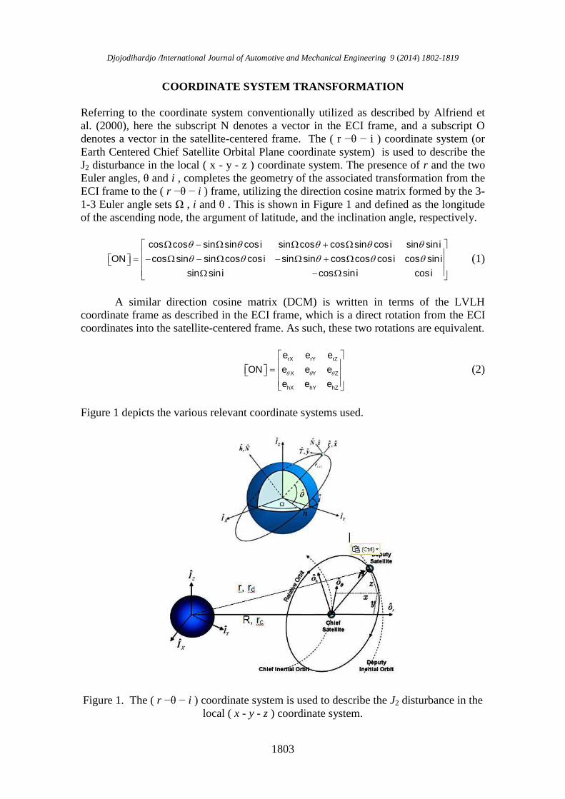
Validation of Clohessy-Wiltshire Model To demonstrate the relative satellite motion modeled by the Clohessy-Wiltshire equations, the projected circular orbit trajectory is simulated via MATLAB. The trajectory follows the initial conditions defined by the set of solutions presented in Table 1.
1816
Figure 5. Relative trajectory comparison for ρ= 1km, 5km, 10km, 25km, and 50km with e=0 and a= 7225km.
Figure 6. Clohessy-Wiltshire model error for ρ= 1km, 5km, 10km, 25km, and 50km with e=0 and a= 7225km.
Djojodihardjo /International Journal of Automotive and Mechanical Engineering 9 (2014) 1802-1819
1817
Example and Comparison of Baseline Clohessy-Wiltshire Model of Twin-Satellite Orbits with J2-Perturbed Orbits
(a) (b)
(c) (d) Figure 7. Comparison of Baseline Ground-Track of the Orbits of the Deputy and Chief Satellites. (a) Without J2 Perturbation; (b) With J2 Perturbation (c) Comparison of the radius of the orbit of the Deputy Satellite around the Chief Satellite as the solution of Clohessy-Wiltshire Equation (without J2) and incorporating the influence of J2, using
linearized modified Clohessy-Wiltshire Equation; the influence of J3 is also shown (Djojodihardjo & Haur, 2014). (d) Comparison of the orbit of the Deputy Satellite
around the Chief Satellite as the solution of Clohessy-Wiltshire Equation (without J2) and incorporating the influence of J2, using linearized modified Clohessy-Wiltshire
Equation.
To demonstrate the relative satellite motion modeled by the Clohessy-Wiltshire equations, the projected circular orbit trajectory is simulated via MATLAB. The trajectory follows the initial conditions defined by the set of solutions given by Djojodihardjo et al. (2010). To demonstrate the influence of J2 on the linearized (CW) orbit of the Twin Satellite Formation Flying Orbits, the J2 perturbed linearized CW equations orbits are compared with the baseline orbits. Some examples of the results indicating the influence of J2 are shown in Figure 7.
1818
Table 1. Chief’s Orbital Elements and deputy’s initial conditions with respect to Chief
Chief Satellite
Altitude, h (km) Eccentricity, e Orbit Inclination, I (deg) Right Ascension of the Ascending Node, Ω (deg) Argument of Perigee ω (deg) Mean Anomaly at Epoch, M (deg)
A computation procedure following linearized Clohessy-Wiltshire equations has been developed to allow parametric study of spacecraft formation flying. Some preliminary results will provide basic information relevant to the choice of orbital parameters. Such results also exhibit the merit of simple analysis, which could be extended to incorporate other parameters. The relevance of parametric study as a preliminary step towards optimization efforts has been demonstrated in the presentation of the results. The influence of J2 to the formation flight trajectories for twin satellites consisting of the chief and deputy satellites have also been derived. The relative positions in the LVLH frame will be used to compare the accuracy of the present model with various models in the literature. These will be displayed as errors from the desired relative position in the LVLH or Hill frame.
ACKNOWLEDGEMENTS The author would like to thank Universiti Putra Malaysia (UPM) for granting Research University Grant Scheme (RUGS) Project Code: 9378200, under which the present research was carried out.
REFERENCES
Alfriend, K., Vadali, S. R., Gurfil, P., How, J., & Breger, L. (2010). Spacecraft formation flying: Dynamics, Control, and Navigation (Vol. 2): Butterworth-Heinemann.
Alfriend, K. T., Gim, D.-W., & Schaub, H. (2000). Gravitational perturbations, nonlinearity and circular orbit assumption effects on formation flying control strategies. Guidance and Control 2000, 139-158.
Djojodihardjo /International Journal of Automotive and Mechanical Engineering 9 (2014) 1802-1819
1819
Djojodihardjo, H. (1972). Vinti's surface density as a means of representing the earth's disturbance potential. Proceedings-Institut Teknologi Bandung, 7(4), 139.
Djojodihardjo, H., & Haur, T. J. (2014). An assessment of the influence of j 2 on formation flying of micro-satellites in low orbits. Advanced Science Letters, 20(2), 439-445.
Djojodihardjo, H., Salahuddin, A., & Harithuddin, M. (2010). Spacecraft formation flying for tropical resources and environmental monitoring: A parametric study. Advances in the Astronautical Sciences, 138(49), 2010.
Vinti, J. P. (1971). Representation of the earth's gravitational potential. Celestial Mechanics, 4(3-4), 348-367.
Yeh, H.-H., & Sparks, A. (2000). Geometry and control of satellite formations. Proceedings of the 2000 American Control Conference.