WATER RESOURCES RESEARCH, VOL. 35, NO. 12, PAGES 3747-3759, DECEMBER 1999

Influence of various water quality sampling strategies on load estimates for small streams

Dale M. Robertson and Eric D. Roerish

Water Resources Division, USGS, Middleton, Wisconsin

Abstract. Extensive streamflow and water quality data from eight small streams were systematically subsampled to represent various water-quality sampling strategies. The subsampled data were then used to determine the accuracy and precision of annual load estimates generated by means of a regression approach (typically used for big rivers) and to determine the most effective sampling strategy for small streams. Estimation of annual loads by regression was imprecise regardless of the sampling strategy used; for the most effective strategy, median absolute errors were -30% based on the load estimated with an integration method and all available data, if a regression approach is used with daily average streamflow. The most effective sampling strategy depends on the length of the study. For 1-year studies, fixed-period monthly sampling supplemented by storm chasing was the most effective strategy. For studies of 2 or more years, fixed-period semimonthly sampling resulted in not only the least biased but also the most precise loads. Additional high-flow samples, typically collected to help define the relation between high streamflow and high loads, result in imprecise, overestimated annual loads if these samples are consistently collected early in high-flow events.

1. Introduction

Various approaches have been used to quantify the total transport (load) of specific constituents past a fixed point on a stream. In most of the more accurate approaches it is assumed that discrete water quality samples are collected and that con- tinuous or at least daily average streamflow records are avail- able or can be estimated. The most common approach is to estimate loads by means of continuous (at least daily) concen- tration and streamflow traces. Loads are then estimated by multiplying the continuous concentration trace by the contin- uous streamflow trace. A continuous concentration trace can

be developed by either of two approaches: the integration method and the rating curve, or regression, method. In the integration method, constituent concentrations are plotted through time, and hydrologic judgement is used to extrapolate between the measured concentrations [Porterfield, 1972]. Inte- gration is generally considered to be the most accurate method to estimate loading at all timescales if sufficient data are col- lected to describe the changes in water quality, especially if samples are collected throughout the largest high-flow events during the period of interest. It is difficult, however, to place confidence limits on loads estimated with this approach. For accurate load estimations, "sufficient data" often means that many samples must be collected to reflect the variability in water quality; thus the integration method is the most expen- sive approach. Loads calculated by use of this method are often used as a reference to evaluate results from other methods.

The regression method usually uses a relation found be- tween concentration (or load) and daily average flow (and other independent variables) to estimate daily concentrations (or loads) of the constituent, although it has also been applied using instantaneous and hourly average flows. The regression

This paper is not subject to U.S. copyright. Published in 1999 by the American Geophysical Union.

Paper number 1999WR900277.

method began as simple linear relations between concentra- tion (or load) and flow but has been modified to account for nonlinearities, seasonal and long-term variability, censored data, biases associated with using logarithmic transformations, and serial correlations in the residuals of the analyses [Cohn, 1995]. This approach has come into widespread use because it requires'less data than integration does, produces estimates for periods beyond when concentration data were collected, and enables confidence limits to be placed on the estimates. The regression method is often used with very small data sets that have been assembled over several years.

With the regression method one typically uses daily average streamflow to estimate daily average concentrations (or loads) because this is the resolution of most streamflow databases.

Therefore each concentration and streamflow combination

(and any other independent variable) used in the regression is assumed to be representative of the average daily conditions when the data were collected. Instantaneous flows are com-

monly measured during sampling; however, these data are not usually used in the analysis because the daily average flows are used with the regression equations to estimate total loads and confidence limits. In this type of analysis, if more than one sample was collected during a given day, each concentration would be assigned the same daily average flow. Therefore high-flow samples should be randomly collected throughout the day during high-flow events. This type of regression ap- proach is usually considered to be a "big river" approach be- cause it is based on the assumption that samples represent the daily average concentration and it estimates changes in con- centration (or loads) on a daily time step. However, this ap- proach has been commonly used to estimate loads in small streams in which concentrations can change rapidly [Walker, 1996].

Because of financial constraints the number of samples that can be collected and analyzed is often limited. Therefore sam- pling for the integration approach is usually designed to collect

3747

3748 ROBERTSON AND ROERISH: INFLUENCE OF SAMPLING STRATEGIES

I--

rr I-- Z

Z

I i i i i i i I I I i i i i i i i i I I I I I I I

Bower Creek

East River

Bower Creek (East River Sampling Frequency)

I i i i i i i_

OND J FMAM J J ASOND J FMAMJ J ASOND 1992 1993 1994

Figure 1. Effects of sampling strategy on number and distri- bution of samples for two small streams. Intensive sampling was used at Bower Creek, Wisconsin, and fixed-period sam- pling supplemented with a few high-flow samples at East River, Wisconsin.

samples rather sparsely when concentrations are thought to be stable (such as during base flow) and intensely when concen- trations are thought to be changing (such as during high flow). An example of data collected in this manner is shown for Bower Creek, Wisconsin, in Figure 1. In most studies the sampling budget requires more restrictive sampling (shown in Figure 1 for the East River, Wisconsin). The similarity in water quality of the two streams can be inferred by examining just the Bower Creek data collected with the East River sampling fre- quency. Infrequent sampling is often inadequate to directly describe the changes in water quality and usually misses the highest concentrations. Therefore the infrequent data must be used to extrapolate concentrations during most of the time period.

How well infrequently collected data, such as that collected for the East River, can be extrapolated to the entire time period depends on how well the changes in concentration are related to other independent variables. Concentrations of many constituents have been shown to be directly related to streamflow. For many constituents, concentrations increase very rapidly during increasing flow, peak prior to maximum flow, and then decrease more slowly during decreasing flow (hysteresis). These general changes in concentration associ- ated with changes in flow are characteristic of sediment, total phosphorus, pesticides, and other sediment-derived constitu- ents [Richards and Holloway, 1987; Richards and Baker, 1993]. Concentrations of other constituents, such as nitrates or chlo- rides or constituents from point sources, often decrease with increasing flow because of dilution. How quickly concentra- tions change in a stream often depends on the variability in flow, which in turn depends on the size of the basin and the surficial deposits, slope of the terrain, and land use in the basin. In some small streams, flow and concentrations increase to very high levels and decrease back to baseline within 1 day. Changes in streamflow and total phosphorus concentrations during a high-flow event in Bower Creek are shown in Figure 2.

The goal of this analysis is to determine the most effective sampling strategy for computing loads in small streams when

only limited samples can be collected, and therefore the re- gression method is used.

1.1. Sampling Strategies

Various sampling strategies have been used to collect data to estimate loads to take advantage of the systematic or nonsys- tematic changes in concentration. A full integration design typically includes fixed-period, manually collected, monthly or semimonthly samples supplemented with many miscellaneous samples collected during high flows, such as sampling con- ducted by the Nonpoint Program of the U.S. Geological Survey (USGS) Wisconsin District [Graczyk et el., 1993]. Typically, this program collects 100-200 samples per year per site for small streams, i.e., less than ---100 km 2 (Figure 1). Automated equipment is commonly used to collect samples when stream- flow is rapidly changing, especially for small streams. Because the automated equipment can collect nonrepresentative sam- ples, coinciding manual and automated samples are generally collected and correction coefficients are calculated and applied if needed.

Another sampling strategy is to manually collect samples at a fixed interval (monthly or more frequent). The Wisconsin Department of Natural Resources (WDNR) collects samples monthly [Tiegs, 1986] and the Illinois Environmental Protec- tion Agency collects samples every 6 weeks [Illinois Environ- mental Protection Agency, 1996]. Other sampling strategies are between these two extremes and have fixed-period sampling supplemented with a few samples collected during high flows. The typical design of National Water-Quality Assessment (NAWQA) Program [Hirsch et el., 1988], a nationwide sam- pling effort by the USGS, is to collect fixed-period monthly samples supplemented by four to eight manually collected high-flow samples per year for ---2.5 years [Gilliom et el., 1995]. This design results in ---18 samples per year and ---45 samples over 2.5 years for both large rivers and small streams. Loads estimated from these data are often computed by use of a regression approach (D. K. Mueller, USGS, written commu- nication, 1998).

If a regression approach is to be used to compute loads, the additional high-flow samples are usually attempted to be col- lected over a range of flows. How the additional high-flow

40 , , 4 •

• 30

• 20

g

• lO

• 0 ' 0800 1600

8

I Flow

(• ,• -q-' Concentration ji r•lii ,l• Fixed Period !! I [ I Storm Chasing

ii I. • • Peak Flow

i •'••'•r••l" It Single Stags

2400 0800 1600 2400 0800 1600

9 10

June 1993

i.- z LLI

z

2 0

1 0

0

Figure 2. Changes in total phosphorus concentration during a high-flow event in a small stream in 1993 (Bower Creek, Wisconsin). Samples collected for various sampling strategies are identified with respect to flow and concentration.

ROBERTSON AND ROERISH: INFLUENCE OF SAMPLING STRATEGIES 3749

samples are collected and how many event• are sampled de- pend on resources. With limited high-flow sampling, the addi- tional samples are usually collected manually when a sampling crew can get to the stream or by use of single-stage samplers that collect a sample as the water level exceeds a given storm stage [Edwards and Glysson, 1988]. In slowly responding big rivers, samples can easily be collected throughout the changes in the hydrograph. In small flashy streams, however, a sampling crew chasing storms might be expected to collect samples later in the events, resulting in a bias toward lower concentrations, whereas automated sampling techniques like single-stage sam- plers collect samples earlier in the event and might be biased toward higher concentrations. Fixed-period sampling usually results in random samples collected throughout a range in streamflows, but because high flows are infrequent, they are generally underrepresented.

Although sampling strategies vary among monitoring pro- grams, many programs have a common goal: to estimate the total load of various constituents transported in the stream. Regression methods are probably the most common approach for estimating loads because the infrequent data collected in most monitoring programs require concentrations and loads to be estimated during the large gaps between samplings. Use of regression methods poses certain questions: How accurate are regression techniques with infrequent data, especially for small streams? How do various sampling strategies affect this accuracy?

1.2. Accuracy in Load Estimates

The accuracy of the regression approach at estimating an- nual loads has been evaluated in only a few cases. Walling and Webb [1981] used hourly suspended sediment data, derived from continuous turbidity measurements, collected over 7 years to estimate "true" annual sediment loads for a small stream in the United Kingdom, using the integration approach. These data were then used to determine the accuracy and precision of the regression approach using subsamples of these data chosen on the basis of fixed intervals (1-14 days) and a fixed interval (7 days) supplemented with additional random samples collected during high flows. Between 365 and 1365 samples were used to calibrate simple exponential models us- ing both hourly and daily streamflow. They found that the regression approach using either hourly and daily average streamflow consistently underestimated the annual sediment load by 23-83%. Walling and Webb [1988] obtained similar results for other small streams and found that the bias could

not be easily corrected for by use of transformation adjustments. Dolan et al. [1981] and Preston et al. [1989] evaluated the

regression approach for two large rivers (Grand and Saginaw Rivers). Virtually daily data were used to estimate a true load using the integration approach. These values were compared with estimates made by the regression approach using daily average streamflow and randomly selected subsets of the water quality data (12 samples to represent monthly, 4 to represent quarterly, etc.) or stratified random data sets (randomly monthly plus randomly during high flows) by means of Monte Carlo methods. They demonstrated average biases and stan- dard deviation in the errors in annual total phosphorus loads to be <10% when using -24 samples a year. They found only very minor improvement in the estimates when substituting 12 monthly samples plus 12 event samples for the 24 semimonthly samples. In general, the regression approach (with the im- provements described by Cohn [1995]) has been shown to provide nearly unbiased estimates with relatively low variance

for large rivers, although in some cases very large errors can result [Cohn et al., 1992].

As part of the Nonpoint Program of the USGS and WDNR, extensive phosphorus and suspended solids and sediment data were collected for several small streams in Wisconsin [Owens et al., 1997]. At each site, samples were collected at fixed intervals and throughout most high-flow events. These data were used to estimate phosphorus and suspended solids and sediment loads by use of the integration approach [Porterfield, 1972]. In this paper, we use various sampling strategies to subsample the data collected for eight of these streams and then use the regression approach using daily average flow to compute an- nual loads for each stream [Cohn et al., 1989]. In other studies that have examined how various sampling strategies affect load computations, subsampling was done at a fixed interval or in some random order, such as randomly throughout the entire data set or randomly during low and high flows, and often, many samples were used to derive the regression relations. However, in this study, subsets were based on specifically de- fined sampling protocols, similar to protocols actually used by sampling crews and limited in number to what is often col- lected. Load estimates generated from subsets of the data are compared with those computed with the integration method to determine the accuracy and precision of regression techniques using daily average flow, which is often used for small streams with infrequent data and to determine how the accuracy and precision changes with various sampling strategies. We then compare this accuracy with the flashiness of the streams to see whether the most effective sampling strategy for small streams depends on their relative responsiveness in flow.

2. Study Sites and Methods 2.1. Study Sites

The eight small streams are located in agricultural areas of the southern half of Wisconsin and have drainage areas that range in size from 14 to 110 km 2 (Table 1). Each site was instrumented to continuously record water levels and compute flow by use of a stage-discharge relation. Water samples were collected manually at fixed intervals (approximately every 2 weeks from March through October and monthly in other months) by use of the equal width increment (EWI) method described by Guy and Norman [1970] and throughout high-flow events by use of stage-activated, refrigerated, automatic sam- plers [Graczyk et al., 1993]. At each site between -90 and 195 water samples were collected each year (Table 1; -20 fixed- period samples and usually 6-10 samples in each of -10-20 storms annually) and analyzed for total phosphorus (TP) and either suspended solids or suspended sediment (Table 1). In the analysis, annual loads of suspended solids and suspended sediment were combined and referred to as "SS." All chemical

analyses were done by the Wisconsin State Laboratory of Hy- giene in accordance with the guidelines of the U.S. Environ- mental Protection Agency [Wisconsin State Laboratory of Hy- giene, 1993] or by USGS water quality laboratories in accordance with standard analytical procedures described by Fishman and Friedman [1989]. A detailed summary of collec- tion procedures and quality assurance and quality control is given by Graczyk et al. [1993]. A few EWI samples were col- lected concurrently with automated samples to develop coef- ficients to correct for concentration differences between the

automatic samplers and the more representative integrated EWI samples. Correction coefficients, computed as the ratio of

3750 ROBERTSON AND ROERISH: INFLUENCE OF SAMPLING STRATEGIES

Table 1. Characteristics of Eight Streams Used in This Study

Site Name

U.S. Geological Drainage Flashiness Average Survey Station Area, Index, Relative

Number km2 Qs/Q 95 Flashiness Rank Constituents*

Average Number of Samples per Year

Bower Creek 04085119 38.3 415.0 1.0

Brewery Creek 05406470 27.2 41.2 2.0 Eagle Creek 05378185 37.0 3.4 7.7 Garfoot Creek 05406491 14.0 4.4 6.7

Joos Valley Creek 05378183 15.3 3.5 6.7 Kuenster Creek 054134435 24.9 7.6 4.7 Otter Creek 040857005 24.6 12.0 3.0 Rattlesnake Creek 05413449 109.8 8.0 4.3

TP/solids TP/sediment TP/solids TP/sediment TP/solids TP/solids TP/solids TP/solids

195

100

100

93 107

98

172 117

Here Qs/Q95 is the ratio of the 5th and 95th percentiles of flow. *TP is total phosphorus, solids is suspended solids, and sediment is suspended sediment.

the EWI sample to the automated sample, ranged from 0.9 to 1.0. Data collection periods for these sites vary, but each was sampled during 1992-1994. Included in this period was a rel- atively dry year (1992), a relatively wet year (1993), and a relatively normal year (1994).

The responsiveness of flow differed widely among the streams because of the differences in surficial deposits and slopes of the terrain in the watersheds [Rappold et al., 1997]. To quantify this variability, three flow responsiveness indices were computed by taking the ratio of various percentiles of flow: Qs/Q95 (5th/95th percentile of flow), Q•o/Q9o, and Q2o/Q8o [Richards, 1990]. The Qs/Q95 ratio and the relative ranking of the eight sites on the basis of an average ranking from the three ratios are given in Table 1.

2.2. Sampling Strategies and Subsampling of Data Set

To simulate data collected using sampling strategies that are less intensive than used for the full integration method, the chemistry time series of each stream was systematically sub- sampled. Ten sampling strategies were simulated for TP. Three were fixed-period strategies (semimonthly, monthly, and every 6 weeks). Seven involved fixed-period plus high-flow samples (semimonthly plus high-flow (storm-chasing) samples, semimonthly plus single-stage samples, monthly plus storm- chasing samples, monthly plus peak flow samples, monthly plus single-stage samples, 6-week plus storm-chasing samples, and 6-week plus single-stage samples). Seven sampling strategies were used for SS. Two were fixed-period strategies (semi- monthly and monthly), and five involved fixed-period plus high-flow samples (semimonthly plus storm-chasing samples, semimonthly plus single-stage samples, monthly plus storm- chasing samples, monthly plus peak flow samples, and monthly plus single-stage samples).

Fixed-period monthly sampling was simulated by use of the sample collected at the most frequently sampled time of the month in the entire period. Semimonthly sampling was simu- lated with the monthly sample plus a second sample -15 days away from the monthly sample. Six-week sampling was simu- lated with every third sample in the semimonthly data set, unless a biweekly sample was missing, such as often occurred during winter. If more than one sample was collected on any of these dates, the sample collected closest to 11:00 A.M. CT was chosen (midmorning was when most manual samples were collected).

After testing various protocols, the following strategy was selected to subsample high-flow events in an unbiased manner and provide, on average, approximately six to nine high-flow

samples per year. The first step was to determine flow thresh- olds for a high-flow event that become more stringent with many events (such as during a wet year) and less stringent with dry conditions:

1. For the base threshold, compute the flow at the 99th percentile of flow from existing flow data, i.e., the daily average flow that is exceeded only 1% of the time (TB).

2. For a more stringent threshold, multiply TB by 2 (TM•). 3. For the most stringent threshold, multiply Ta by 4

4. For a less stringent threshold, multiply Ta by 0.75

5. For the least stringent threshold, multiply Ta by 0.50

The second step was to select the samples appropriate for the various sampling strategies by examining the 15-min flow data stored in the USGS Automated Data-Processing System (ADAPS) within the National Water Information System (NWlS) [USGS, 1998]. To decide which samples would have been collected by a storm-chasing crew, a sample was chosen when the instantaneous 15-min flow surpassed the high-flow thresholds between 6:00 A.M. and 4:00 P.M. (typical work hours). In examining the 15-min flow data, future flow data were not examined (because a sampling crew would not have this information). It was assumed that only one sample was collected in any high-flow event, as would be typical of most monitoring programs. In each year the sampling clock began on January 1 with an initial threshold set to Ta. Because TB represented the daily flow exceeded 1% of the time, it was exceeded more frequently for instantaneous flows. If the streamflow exceeded Ta, the sampling crew would assumedly take -2 hours to reach the stream, so the sample collected closest to 2 hours after flow exceeded Ta was chosen. Once a sample was chosen in a month, the threshold became more stringent for the next high-flow event in that month because a sampling crew would not want to use its total budget in a single month. Therefore the threshold was set to TM•, similar to what may be actually done. If a second sample was selected in a given month, the threshold was raised to T•2 for the next event. If conditions were dry and 2 full months passed without selection of a high-flow sample, the threshold was relaxed to Tz• • to try to ensure that high-flow samples would be collected. If 4 full months passed without selection of a high-flow sample, the threshold was further relaxed to Tz•2. Once the first high- flow sample of a month was collected, the threshold was always set to T• and set to Ta the following month. These protocols generally resulted in slightly less than six high-flow samples per

ROBERTSON AND ROERISH: INFLUENCE OF SAMPLING STRATEGIES 3751

year in a dry year and slightly more than six high-flow samples in a wet year.

One strategy that is sometimes attempted for collecting sam- ples over the widest range in flow conditions is to try to collect samples at peak flow in specific high-flow events. This is next to impossible to do in reality without collecting several samples, but it could be simulated in this study. Therefore the sample collected nearest peak flow, regardless of the time of day, was chosen for each high-flow event sampled by the hypothetical storm-chasing crew.

Another strategy to collect high-flow samples is to use sin- gle-stage samplers. For this strategy the samplers were simu- lated to be set at depths equivalent to flows of T B, TM•, and TM2. Samples were then selected closest to when the flow first exceeded these thresholds regardless of the time of day. Only one sample per month was selected for each threshold, and a maximum of three samples were selected for each threshold per year; therefore a maximum of nine single-stage samples were chosen each year. Replicate data sets for each strategy could not be generated because of the very specific sampling strategies simulated.

2.3. Load Computation

Daily, event, and annual loads for TP and SS were previously computed for each site by use of the integration method de- scribed by Porterfield [1972]. All water quality data and daily, monthly, and annual streamflow and loads were publi.shed in annual USGS reports and stored in NWIS databases.

Annual loads for TP and SS were estimated for three study periods to simulate the length of typical monitoring studies: 1 year (dry (1992) and wet (1993)), 2 years (1992-1993), and 3 years (1992-1994). Only 6 months of data were used for 1994 to simulate the typical 2.5-year sampling period of NAWQA. Annual loads (calculated by summing daily loads) and annual standard errors of the predictions of those loads (calculated using daily standard errors of the predictions) were estimated by a regression approach by use of the Estimator program [Cohn et al., 1989]. In this study, estimated daily loads L were computed based on the relations between constituent load (in kilograms) and two variables: streamflow Q (in cubic meters per day) and time of the year T (in radians). The general form of the model was

log (L) = a + b[log (Q) - c] + d[log (Q) - c] 2

+ e (sin T) + f(cos r). (1)

Values for the regression coefficients (a, b, c, d, e, and f) in (1) were computed for each site and for each time period by the use of multiple regression analyses between daily loads (daily average streamflows multiplied by instantaneous mea- sured concentrations, in milligrams per liter) and daily stream- flows Q and time of the year T. For each sampling strategy and for each time interval, only terms that were significant at P < 0.05 were included in the regression. Because a logarithmic transformation was used in (1), daily loads were adjusted to account for a retransformation bias by use of the minimum variance unbiased estimate (MVUE) procedure (see Cohn et al. [1989] for a complete discussion).

2.4. Evaluation Methods

Two approaches are typically used to evaluate the results generated using regression equations. The first compares the magnitude of the standard errors in the predictions from var-

ious regression equations. The second examines the errors in the loads of the regression equations by comparing the esti- mated loads with the true loads. The standard errors in the

predictions (SEs) are commonly used to place confidence in- tervals on estimates generated by regression equations. There- fore the SEs can be used to compare and evaluate the various strategies to collect the data used in the regressions, and the strategy resulting in the smallest SEs is considered to be best. SEs for each annual load estimate were computed for each regression equation used for each stream for each simulation period. A root-mean-square standard error (RMSSE) was used to combine the SEs estimated for each of the eight streams for each year in the 3-year simulation period (24 in- dividual SEs):

RMSSE = [Sum (SE2)Iø'5/N. (2)

Prior to computing the RMSSEs, all annual SEs were con- verted into a percentage of the true annual load for the specific streams so that each error in an annual load was equally rep- resented.

The SEs of these estimates were dependent only upon the variability between the measured and predicted loads for the days in which data were collected; therefore the SEs may not incorporate all the variability that occurred during unmoni- tored periods or systematic biases incorporated into the data set. The estimated annual loads were compared with the true loads to try to incorporate all of the errors. The overall errors were dependent on the magnitude of two components: accu- racy and precision. In this study, the true annual loads were computed by the integration approach, using all of the data available for the defined periods. The accuracy or bias repre- sents the average or median difference between the estimates and the true values. The precision represents the measure of the spread or variance of the errors (0 -2 , computed as the standard deviation of the errors squared). These two compo- nents were combined into one overall estimated error called

the normalized mean square error (MSE) [Preston et al., 1989]:

MSE = Bias 2 + o -2. (3)

The overall errors of the various approaches were also com- pared using median absolute errors (MAEs) and average ab- solute errors (AAEs). To combine the errors for the eight streams and allow comparison among streams and years, all loads were converted to yields (load per unit area), and errors (MSE, bias, SE, MAE, and AAE) were normalized as percent- age of the true annual yield as determined by the integration method.

3. Results 3.1. "True" Yield Estimations

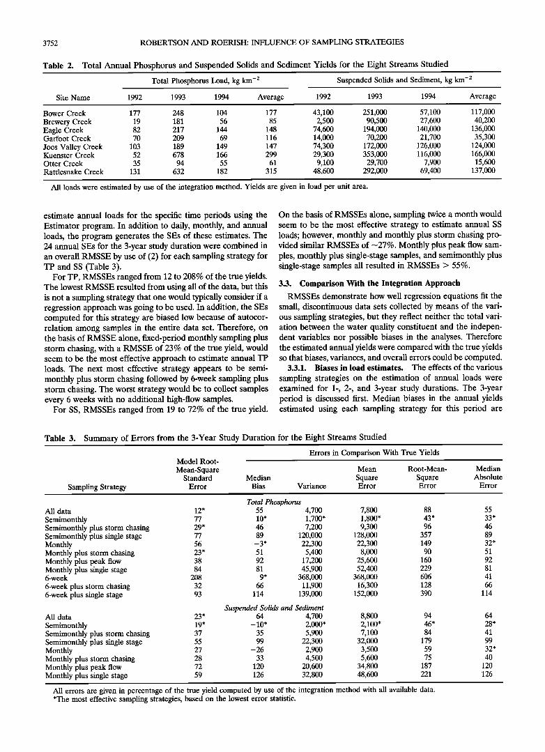
Annual yields for each of the eight sites were computed using all of the data collected at each site during 1992-1994 using the integration method (Table 2). The annual TP yields ranged from 19 to 678 kg km -2 (average annual yields ranged from 61 to 315 kg km-2), and SS yields ranged from 2500 to 353,000 kg km -2 (average annual yields ranged from 15,600 to 137,000 kg km-2). For each stream the highest annual yield occurred in 1993 (wet year), and in most cases the lowest annual yield occurred in 1992 (dry year).

3.2. Comparison of Errors in the Predictions

Subsets of the data, representing those that would have been collected using the various sampling strategies, were used to

3752 ROBERTSON AND ROERISH: INFLUENCE OF SAMPLING STRATEGIES

Table 2. Total Annual Phosphorus and Suspended Solids and Sediment Yields for the Eight Streams Studied

Total Phosphorus Load, kg kn1-2 Suspended Solids and Sediment, kg kn1-2

Site Name 1992 1993 1994 Average 1992 1993 1994 Average

Bower Creek 177 248 104 177 43,100 251,000 57,100 Brewery Creek 19 181 56 85 2,500 90,500 27,600 Eagle Creek 82 217 144 148 74,600 194,000 140,000 Garfoot Creek 70 209 69 116 14,000 70,200 21,700 Joos Valley Creek 103 189 149 147 74,300 172,000 126,000 Kuenster Creek 52 678 166 299 29,300 353,000 116,000 Otter Creek 35 94 55 61 9,100 29,700 7,900 Rattlesnake Creek 131 632 182 315 48,600 292,000 69,400

117,000 40,200

136,000 35,300

124,000 166,000

15,600 137,000

All loads were estimated by use of the integration method. Yields are given in load per unit area.

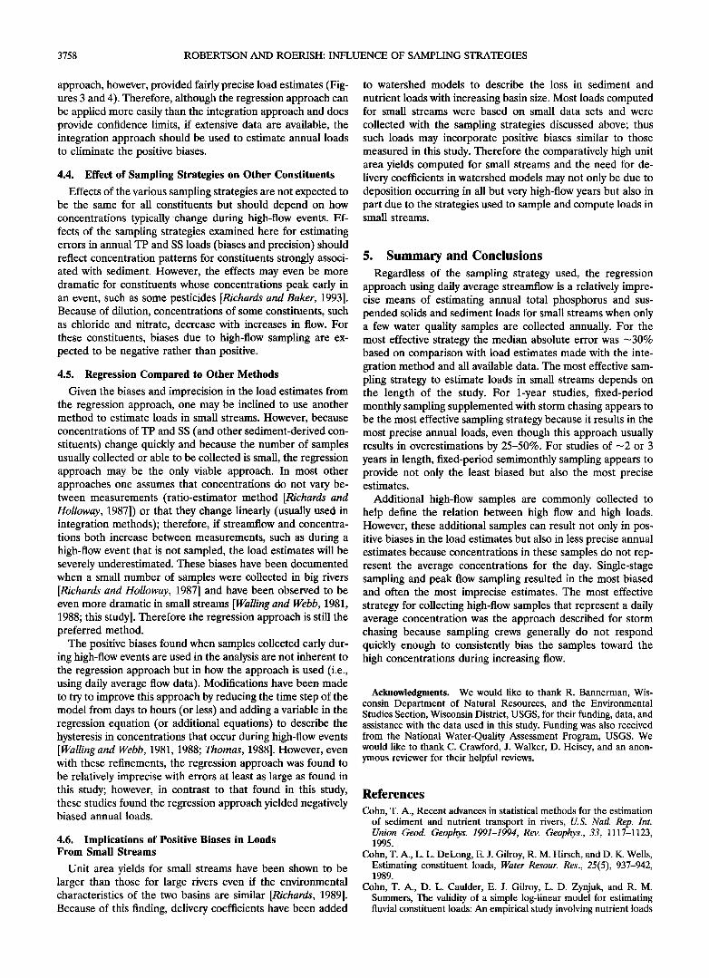
estimate annual loads for the specific time periods using the Estimator program. In addition to daily, monthly, and annual loads, the program generates the SEs of these estimates. The 24 annual SEs for the 3-year study duration were combined in an overall RMSSE by use of (2) for each sampling strategy for TP and SS (Table 3).

For TP, RMSSEs ranged from 12 to 208% of the true yields. The lowest RMSSE resulted from using all of the data, but this is not a sampling strategy that one would typically consider if a regression approach was going to be used. In addition, the SEs computed for this strategy are biased low because of autocor- relation among samples in the entire data set. Therefore, on the basis of RMSSE alone, fixed-period monthly sampling plus storm chasing, with a RMSSE of 23% of the true yield, would seem to be the most effective approach to estimate annual TP loads. The next most effective strategy appears to be semi- monthly plus storm chasing followed by 6-week sampling plus storm chasing. The worst strategy would be to collect samples every 6 weeks with no additional high-flow samples.

For SS, RMSSEs ranged from 19 to 72% of the true yield.

On the basis of RMSSEs alone, sampling twice a month would seem to be the most effective strategy to estimate annual SS loads; however, monthly and monthly plus storm chasing pro- vided similar RMSSEs of -27%. Monthly plus peak flow sam- ples, monthly plus single-stage samples, and semimonthly plus single-stage samples all resulted in RMSSEs > 55%.

3.3. Comparison With the Integration Approach

RMSSEs demonstrate how well regression equations fit the small, discontinuous data sets collected by means of the vari- ous sampling strategies, but they reflect neither the total vari- ation between the water quality constituent and the indepen- dent variables nor possible biases in the analyses. Therefore the estimated annual yields were compared with the true yields so that biases, variances, and overall errors could be computed.

3.3.1. Biases in load estimates. The effects of the various

sampling strategies on the estimation of annual loads were examined for 1-, 2-, and 3-year study durations. The 3-year period is discussed first. Median biases in the annual yields estimated using each sampling strategy for this period are

Table 3. Summary of Errors from the 3-Year Study Duration for the Eight Streams Studied

Errors in Comparison With True Yields Model Root-

Mean-Square Mean Root-Mean- Standard Median Square Square

Sampling Strategy Error Bias Variance Error Error

Median Absolute

Error

Total Phosphorus All data 12' 55 4,700 7,800 88 Semimonthly 77 10' 1,700' 1,800' 43' Semimonthly plus storm chasing 29* 46 7,200 9,300 96 Semimonthly plus single stage 77 89 120,000 128,000 357 Monthly 56 -3' 22,300 22,300 149 Monthly plus storm chasing 23' 51 5,400 8,000 90 Monthly plus peak flow 38 92 17,200 25,600 160 Monthly plus single stage 84 81 45,900 52,400 229 6-week 208 9' 368,000 368,000 606 6-week plus storm chasing 32 66 11,900 16,300 128 6-week plus single stage 93 114 139,000 152,000 390

Suspended Solids and Sediment All data 23' 64 4,700 8,800 94 S emimonthly 19' - 10* 2,000* 2,100' 46 * Semimonthly plus storm chasing 37 35 5,900 7,100 84 Semimonthly plus single stage 55 99 22,300 32,000 179 Monthly 27 - 26 2,900 3,500 59 Monthly plus storm chasing 28 33 4,500 5,600 75 Monthly plus peak flow 72 120 20,600 34,800 187 Monthly plus single stage 59 126 32,800 48,600 221

55

33* 46

89 32*

51

92

81 41

66 114

64

28* 41

99

32* 40

120 126

All errors are given in percentage of the true yield computed by use of the integration method with all available data. *The most effective sampling strategies, based on the lowest error statistic.

ROBERTSON AND ROERISH: INFLUENCE OF SAMPLING STRATEGIES 3753

140

120

100

• 80

z i,u 60

13. 40

z

•3 20

o

-20

-40

16o

140

120

lOO

80

60

40

20

i i i

-e-, 3 Years

-B- 2 Years

-I•- 1 Year (Dry)

'•)•' 1 Year (Wet)

i i i i i I i i

Total Phosphorus

I I

ALL SM I I

SMPS SMSS MON MPS MPP MSS 6W 6WPS 6WSS

SAMPLING STRATEGY

ALL SM SMPS SMSS

13 Variance

! Bias Squared

MON MPS MPP MSS

SAMPLING STRATEGY

8,0

6W 6WPS 6WSS

Figure 3. Biases (in percent) and mean square errors (in percent squared, which is percent difference from true yield estimated by the integration method) for total phosphorus for various sampling strategies for the eight studied streams. Each group of four bars is given in the following order: 1 year (dry), 1 year (wet), 2 years, and 3 years. The all-data and 6-week strategies were used for the 3-year periods only. (All, all data; SM, semimonthly; SMPS, semimonthly plus storm chasing; SMSS, semimonthly plus single stage; MON, monthly; MPS, monthly plus storm chasing; MPP, monthly plus peak flow; MSS, monthly plus single stage; 6W, 6-week; 6WPS, 6-week plus storm chasing; and 6WSS, 6-week plus single stage.)

shown as bold lines in Figure 3 (TP) and Figure 4 (SS) and are summarized in Table 3. Median biases were used to minimize

the effects of a few outliers. Median biases ranged from almost no bias for some fixed-period sampling strategies to >100% for some strategies with additional high-flow samples. All fixed-period sampling strategies (6-week, monthly, and semi- monthly) resulted in median biases <26% of the true annual yields of TP and SS; however, all yields estimated by use of fixed-period sampling plus any type of high-flow sampling re- sulted in positive biases >33%. All of the biases associated with high-flow sampling were positive, indicating that the es- timated yields were greater than the true yields. In general, examining average (rather than median) biases resulted in the same general conclusions.

The two other sampling period lengths showed similar biases

as those found for the 3-year period: fixed-period sampling resulted in biases less than those produced with additional high-flow samples. In almost all cases, positive biases were largest when fixed-period sampling was supplemented with peak flow or single-stage samples. For TP, almost all of the fixed-period sampling strategies resulted in yields with almost no bias; however, for SS, fixed-period sampling generally re- sulted in negatively biased yields. The largest negative biases for TP and SS were for monthly sampling during a wet year.

When all of the data for each site were used in the regres- sions, there was a positive bias >50%. The mean and median biases were similar.

3.3.2. Variance in yield estimates. A very small bias does not necessarily mean that a sampling strategy produced small errors in annual loads if the variance in estimated yields is very

3754 ROBERTSON AND ROERISH: INFLUENCE OF SAMPLING STRATEGIES

200

150

100

50

0

-50

-100

lOO

z 80

o

v 60

o

uJ 40

(3I

• 20

i i

• 3 Years

-1- 2 Years

-I•- 1 Year (Dry)

'•' 1 Year (Wet)

i i i

Suspended Solids / Sediment

I

ALL

I I I I I I I

SM SMPS SMSS MON MPS MPP MSS SAMPLING STRATEGY

Variance •'•,345,000 Bias Squared

ALL SM SMPS SMSS MON MPS MPP MSS

SAMPLING STRATEGY

Figure 4. Biases (in percent) and mean square errors (in percent squared, which is percent difference from true yield estimated by the integration method) for suspended sediment and solids for various sampling strategies for the eight studied streams. Each group of four bars is given in the following order: 1 year (dry), 1 year (wet), 2 years, and 3 years. The all-data strategy was only used for the 3-year periods.

large. Therefore we examined the variance in the errors in the annual yield estimates (Table 3 and Figures 3 and 4). For the 3-year period (fourth bar in each group in Figures 3 and 4; 6-week strategies were examined for the 3-year period only), the variance in the errors ranged from 1700 to 368,000 for TP and 2000 to 32,800 for SS. For both TP and SS, variance in the errors was lowest for semimonthly sampling. For TP the sec- ond lowest variance was for monthly sampling plus storm chas- ing and the third lowest was for semimonthly sampling plus storm chasing. For SS the second lowest variance was for monthly sampling, and the third lowest was for monthly sam- pling plus storm chasing. All sampling strategies for SS with additional high-flow samples increased the variance. For both TP and SS, high-flow samples collected near peak flow or with single-stage samplers increased the variance from that esti- mated for storm chasing.

Different study durations produced very different variances compared to those found for the 3-year period, but in general,

variances were consistently lowest for monthly or semimonthly sampling supplemented by storm chasing and monthly and semimonthly sampling for longer periods. The magnitude of the variance did not appear to have any consistent relation to the duration of the study. Sometimes 1 year of data resulted in small errors (such as for semimonthly sampling and monthly sampling with storm chasing for both TP and SS) and some- times in large errors (such as for semimonthly sampling for SS). In many cases for TP and SS, combining 2 or 3 years of samples resulted in variances larger than for each of the indi- vidual years, especially if high-flow samples were included. The variances of the errors when all of the data were used in the

regressions were consistently small. 3.3.3. Overall mean square error in yield estimates. To

evaluate the overall errors of the various sampling strategies, the biases and variances were combined into an MSE using (3) (Table 3 and Figures 3 and 4). For the 3-year period the MSEs ranged from -1800 to 368,000 for TP and 2100 to 48,600 for

ROBERTSON AND ROERISH: INFLUENCE OF SAMPLING STRATEGIES 3755

Table 4. Summary of Median Absolute Errors for the Eight Streams Studied

Median Absolute Error, %

Sampling Strategy 1 Year (Dry) 1 Year (Wet) 2 Years 3 Years

Total Phosphorus All data 55

Semimonthly 18 (105)* 26 (26)* 32 (52)* 33 (36)* Semimonthly plus storm chasing 23 (44)* 26 (28)* 43 46 Semimonthly plus single stage 38 67 80 89 Monthly 25 38 40 32 (76)* Monthly plus storm chasing 27 43 54 51 Monthly plus peak flow 51 101 105 92 Monthly plus single stage 53 129 103 81 6-week 41

6-week plus storm chasing 66 6-week plus single stage 114

Suspended Solids and Sediment All data 64

Semimonthly 37 (720)* 51 20 (39)* 28 (35)* Semimonthly plus storm chasing 54 (59)* 24 (25)* 36 41 Semimonthly plus single stage 87 120 108 99 Monthly 50 (54)* 70 45 32 (42)* Monthly plus storm chasing 72 26 (32)* 55 40 Monthly plus peak flow 112 122 170 120 Monthly plus single stage 116 148 133 126

All errors are given in percentage of the true yield computed by use of the integration method with all available data.

*The strategies yielding the lowest MAEs for each period. The average absolute error for the strategy with the lowest MAE for the period is listed in parentheses.

SS. To evaluate the MSEs in terms of an approximate percent error, the root-mean-square error was computed (Table 3). The lowest overall errors then equate to -45% of the true annual yields. For both TP and SS, MSEs were lowest for fixed-period, semimonthly sampling. Monthly sampling plus storm chasing and semimonthly sampling plus storm chasing were in the top four strategies for both TP and SS. In all cases for SS, additional high-flow samples increased the MSEs, es- pecially for peak flow and single-stage samples. MSEs for yields estimated from semimonthly sampling plus storm sam- ples were slightly higher than those from monthly sampling plus storm samples.

Different study durations once again produced very differ- ent MSEs compared to those found for the 3-year period, primarily because the variances of the errors were, in general, much larger than the biases squared. In general, MSEs were consistently lowest for monthly and semimonthly samples sup- plemented with storm chasing and for fixed-period monthly and semimonthly sampling for longer periods; thus these ap- pear to be the most effective overall sampling strategies.

The MSEs, when all of the data were used in the regression, were consistently a little larger than for monthly and semi- monthly sampling and monthly or semimonthly sampling sup- plemented by storm chasing.

3.3.4. Overall median absolute errors. Another way to evaluate which of the sampling strategies provided the best annual load estimates is to compare the median absolute er- rors (MAEs) (Tables 3 and 4). This approach removes the importance of the sign of the error and also removes the sensitivity to outliers. The variance of the errors, previously described, was very sensitive to a few outliers. For the 3-year period the MAEs ranged from -28 to 126%. For both TP and SS the fixed-period monthly and semimonthly sampling re- sulted in the smallest errors, and additional high-flow samples

always increased the MAEs. The largest errors generally re- sulted from the addition of peak flow and single-stage samples.

For all sampling period lengths (Table 4), semimonthly sam- pling consistently had one of the smallest MAEs; however, MAEs were comparable for semimonthly sampling plus storm chasing for 1-year periods and for monthly sampling for greater than 2-year periods. For all sampling durations, addi- tional peak flow and single-stage samples resulted in the larg- est MAEs.

3.4. Effects of Stream Flashiness on Errors

Larger biases and overall errors in load estimations might be expected for more flashy streams than for less flashy streams. To test this hypothesis, the average absolute error (AAE) for each sampling strategy for the 3-year simulation period was computed (Figure 5). An AAE was used rather than an MSE because only three errors in annual loads were used for each point (insufficient to compute an accurate variance). As evi- dent from Figure 5, the AAEs appear to be unrelated to the relative flashiness of the stream. The AAEs for Bower and

Brewery Creeks (the two flashiest streams with thick lines in Figure 5) generally bracketed the AAEs for the rest of the streams.

In a few cases the regression approach very poorly simulated the actual yields. For Brewery Creek the addition of single- stage, high-flow samples resulted in very large errors, especially for TP. For Kuenster Creek, very large errors occurred in TP yield estimates for 6-week and monthly sampling; these errors were greatly reduced with additional fixed-period samples (semimonthly) or additional storm-chasing samples. Because of the very large errors in just a few cases, especially for TP, median biases and median absolute errors appear to be an appropriate statistic to use in comparing sampling strategies. These few very large errors explain the wide range in variances

3756 ROBERTSON AND ROERISH: INFLUENCE OF SAMPLING STRATEGIES

800

0

fl. •00

0

I-- 400

LI,I 200

i I i i i i i

Total Phosphorus

.... _/......i ß

ALL SM SMPS SMSS MON MPS MPP MSS

I I I I I I I I I I

I I t I

I

I

t

I

t

I

I

.[].

ß

6W 6WS 6WSS

400

Z

0

13. 300

0

I- 200

0

I,M 100

i I i

Relative Flashiness

• Bower-l.0

• Brewery- 2.0

='=(•"" Otter - 3.0

=,-•=,. Rattle - 4.3

--"•-- Kuenster - 4.7

--=•"- Garfoot - 6.7

..... '<:•)' .... Joos - 6.7

<•..: .... E3 ..... Eagle - 7.7

i i i

Suspended Solids/Sediment

0 I I pI I I I ALL SM SMPS S SS MON MPS MPP MSS

Sampling Strategy

Figure 5. Average absolute errors (percent difference from true yield estimated by the integration method) for total phosphorus and suspended sediment and solids for the eight studied streams. The relative flashiness of each stream is identified on Figure 5.

shown in Figures 3 and 4 and the differences in the rankings of the strategies relative to median absolute errors and variance in errors or MSEs.

4. Discussion

4.1. True Loads Versus Actual Loads

The actual load in any stream cannot be determined exactly without accurate continuously recorded flow and concentra- tion data. The data used to estimate the true loads (and yields) in this study were collected as continuously as economically possible: fixed-period samples were collected throughout the entire period (at least semimonthly during the open water period and monthly during winter) and throughout most high- flow events [Graczyk et al., 1993]. Therefore use of the inte- gration method to compute loads with these data is thought to provide the best approximation possible. Changes in concen- tration between high-flow events are thought to be small, but even if concentrations did change, the effect on annual loads would not be large because of the low flow between events.

Analytical errors and errors in estimating flow do not affect the results of comparisons presented here because the same data were used by all of the approaches to estimate loads. A slight systematic bias, however, may have been inadvertently introduced through the use of raw water quality data stored in the USGS database. In computing a few annual loads with the integration approach, correction coefficients were applied to some samples collected with automated samplers. These coef- ficients were always <10% and involved <20% of the load years. Therefore the line of reference in Figures 3 and 4 may be shifted very slightly upward, resulting in negative biases increasing slightly and positive biases decreasing slightly.

4.2. Most Effective Sampling Strategy

The results summarized in Tables 3 and 4 and Figures 3-5 can be used to suggest the most effective strategy for sampling small streams and estimating the magnitude of errors that may be expected when a regression approach is used to estimate loads in flashy streams with small drainage areas (less than ---100 km2). Regardless of the sampling strategy used, use of

ROBERTSON AND ROERISH: INFLUENCE OF SAMPLING STRATEGIES 3757

the regression approach to estimate annual TP and SS loads for small flashy streams with a small number of samples per year (-30 or less) is inherently imprecise and can result in significant biases in annual load estimates. The smallest errors one can expect with either 1 or 2 years of data are -20-40% (median errors, average absolute errors, and approximately the standard deviation of the errors); additionally, with only 1 year of data, estimates can occasionally be very poor (compare the median and mean values in Table 4). With >2 years of data the very poor estimates appear to be eliminated, but the smallest errors one can expect remains -30% (median and average absolute errors) with a standard deviation in the errors of -40-45% (square root of the variance). The magnitude of the errors found in this study is larger than those found using the regression approach for large rivers [Dolan et al., 1981; Preston et al., 1989] but of similar magnitude to that found for smaller streams using either hourly or daily average streamflow in the regression [Walling and Webb, 1981, 1988]. However, Walling and Webb found consistent negative biases in the estimated annual loads using the regression approach compared to the positive biases found in this study.

So, given a limited budget, what is the most effective sam- pling strategy to estimate loads in small, flashy streams? On the basis of the results from this study the answer depends on the length of the study and the reason for estimating those loads. If the length of the study is >2 years, fixed-period, semi- monthly sampling typically produces the smallest errors (least biased and most precise) and therefore is the most effective sampling strategy (see Figures 3 and 4 and Table 3). With >3 years of data it is expected that fixed-period monthly and semimonthly sampling should result in similar errors, so fixed- period monthly sampling may be the most effective sampling strategy. However, longer in-depth studies are needed to com- pare these strategies. Therefore, for long-term monitoring studies that do not require load estimates in the first few years of the study, fixed-period sampling would be an appropriate sampling strategy to estimate annual loads that are unbiased and as precise as those estimated with additional high-flow samples.

If the length of the study is 2 years or less, determining which sampling strategy is most effective is more complicated: one must weigh the tradeoffs between biased estimates and impre- cise estimates. All three fixed-period sampling strategies (6- week, monthly, and semimonthly) provided relatively unbiased load estimates with a regression approach; however, the vari- ance in the errors in annual loads with these strategies was often quite large and much larger than the typical interannual variability in the annual loads of a small stream. Fixed-period monthly and semimonthly sampling plus storm chasing, on the other hand, provided relatively precise estimates for all study lengths, but loads were overestimated by typically 30-50%. Therefore, because interannual variability in annual loads is generally much greater than 30-50%, the most effective sam- pling strategy for 1-year studies appears to be fixed-period monthly or semimonthly sampling supplemented with storm chasing (see Figures 3 and 4). Semimonthly sampling plus storm chasing appeared to provide slightly smaller overesti- mates and more precise annual loads than those estimated with monthly sampling plus storm chasing; however, the improve- ment in load estimates was comparatively small in return for almost doubling the sampling effort. Therefore the most effec- tive sampling strategy for 1-year studies is monthly sampling plus storm chasing. For 2-year studies, semimonthly sampling

and monthly and semimonthly sampling plus storm chasing produced similar overall errors (mean square errors). There- fore, because semimonthly sampling (without additional high- flow samples) produced similarly precise estimates as the other two strategies without consistently overestimating the annual loads, it is the most effective strategy for 2-year studies.

4.3. Effects of Different High-Flow Sampling Strategies

When using the regression approach to compute annual loads, the primary reason to collect additional high-flow sam- ples is to help define the relation between high streamflows and high loads. In theory, one would hypothesize that addi- tional samples during high-flow events, regardless of how or when they were collected, would be better than having no additional samples. However, this study indicates these addi- tional samples can result in not only a positive bias in the annual loads estimates but also less precise overall annual estimates. When using the big river approach, one assumes that each concentration is representative of the daily average streamflow. This is a valid assumption if samples are collected at fixed periods or randomly with respect to flow. In general, the more random samples over a range in flow conditions, the better the overall data set approximates the true values. This is the reason that loads estimated from fixed-period, semi- monthly samples were better than those from monthly sam- ples. Semimonthly samples are more likely to be collected during the infrequent high flows than monthly samples; how- ever, it becomes a tradeoff between cost per sample and in- creased accuracy.

So why do additional high-flow samples result in positive biases and reduced load precision instead of increased accu- racy? The primary reason is that the measured concentrations were generally higher than the actual average daily concentra- tion during the high-flow event. Measured concentrations typ- ically represent what occurs with the much higher flows early in the event; they do not represent the day on the whole, as some random sample would more likely do. When using the big river approach, samples should be randomly collected during high- flow days rather than during parts of the events. For small streams, strategies that result in the least random samples on high-flow days are the samples collected with single-stage sam- plers and at peak flow (see Figures 1 and 2). The most effective strategy examined here to collect high-flow samples is the approach described for storm chasing by sampling crews. Al- though the goal of such sampling typically is to collect samples during the highest flows, samples are usually collected when flow is decreasing and when concentrations represent the daily average concentration better than those measured with single- stage samplers or near peak flow. These concentrations are still usually positively biased, but the magnitude of the bias is not as large as with the other approaches. Therefore inability of sam- pling crews to immediately respond to high-flow events results in better load estimates for these types of streams.

When using the integration approach, the sampling goal is to define all of the changes in concentration. When done most cost effectively, this results in many samples when flow and concentrations are changing rapidly and fewer samples when flow and concentrations are changing more slowly (Figure 2). If all of these data are used to compute loads with a regression approach, a positively biased annual load results because, once again, the samples are not randomly collected throughout the day but are more frequent when concentrations are highest. Loads estimated by use of all the data and the regression

3758 ROBERTSON AND ROERISH: INFLUENCE OF SAMPLING STRATEGIES

approach, however, provided fairly precise load estimates (Fig- ures 3 and 4). Therefore, although the regression approach can be applied more easily than the integration approach and does provide confidence limits, if extensive data are available, the integration approach should be used to estimate annual loads to eliminate the positive biases.

4.4. Effect of Sampling Strategies on Other Constituents

Effects of the various sampling strategies are not expected to be the same for all constituents but should depend on how concentrations typically 'change during high-flow events. Ef- fects of the sampling strategies examined here for estimating errors in annual TP and SS loads (biases and precision) should reflect concentration patterns for constituents strongly associ- ated with sediment. However, the effects may even be more dramatic for constituents whose concentrations peak early in an event, such as some pesticides [Richards and Baker, 1993]. Because of dilution, concentrations of some constituents, such as chloride and nitrate, decrease with increases in flow. For these constituents, biases due to high-flow sampling are ex- pected to be negative rather than positive.

4.5. Regression Compared to Other Methods

Given the biases and imprecision in the load estimates from the regression approach, one may be inclined to use another method to estimate loads in small streams. However, because concentrations of TP and SS (and other sediment-derived con- stituents) change quickly and because the number of samples usually collected or able to be collected is small, the regression approach may be the only viable approach. In most other approaches one assumes that concentrations do not vary be- tween measurements (ratio-estimator method [Richards and Holloway, 1987]) or that they change linearly (usually used in integration methods); therefore, if streamflow and concentra- tions both increase between measurements, such as during a high-flow event that is not sampled, the load estimates will be severely underestimated. These biases have been documented when a small number of samples were collected in big rivers [Richards and Holloway, 1987] and have been observed to be even more dramatic in small streams [Walling and Webb, 1981, 1988; this study]. Therefore the regression approach is still the preferred method.

The positive biases found when samples collected early dur- ing high-flow events are used in the analysis are not inherent to the regression approach but in how the approach is used (i.e., using daily average flow data). Modifications have been made to try to improve this approach by reducing the time step of the model from days to hours (or less) and adding a variable in the regression equation (or additional equations) to describe the hysteresis in concentrations that occur during high-flow events [Walling and Webb, 1981, 1988; Thomas, 1988]. However, even with these refinements, the regression approach was found to be relatively imprecise with errors at least as large as found in this study; however, in contrast to that found in this study, these studies found the regression approach yielded negatively biased annual loads.

4.6. Implications of Positive Biases in Loads From Small Streams

Unit area yields for small streams have been shown to be larger than those for large rivers even if the environmental characteristics of the two basins are similar [Richards, 1989]. Because of this finding, delivery coefficients have been added

to watershed models to describe the loss in sediment and

nutrient loads with increasing basin size. Most loads computed for small streams were based on small data sets and were

collected with the sampling strategies discussed above; thus such loads may incorporate positive biases similar to those measured in this study. Therefore the comparatively high unit area yields computed for small streams and the need for de- livery coefficients in watershed models may not only be due to deposition occurring in all but very high-flow years but also in part due to the strategies used to sample and compute loads in small streams.

5. Summary and Conclusions Regardless of the sampling strategy used, the regression

approach using daily average streamflow is a relatively impre- cise means of estimating annual total phosphorus and sus- pended solids and sediment loads for small streams when only a few water quality samples are collected annually. For the most effective strategy the median absolute error was -30% based on comparison with load estimates made with the inte- gration method and all available data. The most effective sam- pling strategy to estimate loads in small streams depends on the length of the study. For 1-year studies, fixed-period monthly sampling supplemented with storm chasing appears to be the most effective sampling strategy because it results in the most precise annual loads, even though this approach usually results in overestimations by 25-50%. For studies of -2 or 3 years in length, fixed-period semimonthly sampling appears to provide not only the least biased but also the most precise estimates.

Additional high-flow samples are commonly collected to help define the relation between high flow and high loads. However, these additional samples can result not only in pos- itive biases in the load estimates but also in less precise annual estimates because concentrations in these samples do not rep- resent the average concentrations for the day. Single-stage sampling and peak flow sampling resulted in the most biased and often the most imprecise estimates. The most effective strategy for collecting high-flow samples that represent a daily average concentration was the approach described for storm chasing because sampling crews generally do not respond quickly enough to consistently bias the samples toward the high concentrations during increasing flow.

Acknowledgments. We would like to thank R. Bannerman, Wis- consin Department of Natural Resources, and the Environmental Studies Section, Wisconsin District, USGS, for their funding, data, and assistance with the data used in this study. Funding was also received from the National Water-Quality Assessment Program, USGS. We would like to thank C. Crawford, J. Walker, D. Heisey, and an anon- ymous reviewer for their helpful reviews.

References

Cohn, T. A., Recent advances in statistical methods for the estimation of sediment and nutrient transport in rivers, U.S. Natl. Rep. Int. Union Geod. Geophys. 1991-1994, Rev. Geophys., 33, 1117-1123, 1995.

Cohn, T. A., L. L. DeLong, E. J. Gilroy, R. M. Hirsch, and D. K. Wells, Estimating constituent loads, Water Resour. Res., 25(5), 937-942, 1989.

Cohn, T. A., D. L. Caulder, E. J. Gilroy, L. D. Zynjuk, and R. M. Summers, The validity of a simple log-linear model for estimating fluvial constituent loads: An empirical study involving nutrient loads

ROBERTSON AND ROERISH: INFLUENCE OF SAMPLING STRATEGIES 3759

entering Chesapeake Bay, Water Resour. Res., 28(9), 2353-2363, 1992.

Dolan, D. M., A. K. Yui, and R. D. Geist, Evaluation of river load estimation methods for total phosphorus, J. Great Lakes Res., 7, 207-214, 1981.

Edwards, T. K., and G. D. Glysson, Field methods of and measure- ment of fluvial sediment, U.S. Geol. Surv. Open File Rep., 86-531,118 pp., 1988.

Fishman, M. J., and L. C. Friedman (Eds.), Methods for determination of inorganic substances in water and fluvial sediments, U.S. Geol. Surv. Techniques of Water Resour. Invest., book 5, chapter A1, 545 pp., 1989.

Gilliom, R. J., W. M. Alley, and M. E. Gurtz, Design of the National Water-Quality Assessment program: Occurrence and distribution of water-quality conditions, U.S. Geol. Surv. Circ., 1112, 33 pp., 1995.

Graczyk, D. J., J. F. Walker, S. R. Greb, S. R. Corsi, and D. W. Owens, Evaluation of nonpoint-source contamination, Wisconsin: Selected data for 1992 water year, U.S. Geol. Surv. Open File Rep., 93-630, 48 pp., 1993.

Guy, H. P., and V. W. Norman, Field methods for measurement of fluvial sediment, U.S. Geol. Surv. Water Resour. Invest. Rep., book 3, chapter C2, 59 pp., 1970.

Hirsch, R. M., W. M. Alley, and W. G. Wilber, Concepts for a National Water-C)uality Assessment program, U.S. Geol. Surv. Circ., 1021, 42 pp., 1988.

Illinois Environmental Protection Agency, Illinois water quality report, 1994 and 1995, vol. 1, IEPA/BOW/96-O60a, Bureau of Water, Spring- field, 1996.

Owens, D. W., S. R. Corsi, and K. F. Rappold, Evaluation of nonpoint- source contamination, Wisconsin: Selected topics for water year 1995, U.S. Geol. Surv. Open File Rep., 96-661A, 41 pp., 1997.

Porterfield, G., Computation of fluvial-sediment discharge, U.S. Geol. Surv. Water Resour. Invest. Rep., book 3, chapter C3, 66 pp., 1972.

Preston, S. D., V. J. Bierman Jr., and S. E. Silliman, An evaluation of methods for the estimation of tributary mass loads, Water Resour. Res., 25(6), i379-1389, 1989.

Rappold, K. F., J. A. Wierl, and F. U. Amerson, Watershed charac- teristics and land management in the nonpoint-source evaluation monitoring watersheds in Wisconsin, U.S. Geol. Surv. Open File Rep., 97-110, 39 pp., 1997.

Richards, R. P., Evaluation of some approaches to estimating non- point pollutant loads for unmonitored areas, Water Resour. Bull., 25(4), 891-904, 1989.

Richards, R. P., Measures of flow variability and a new flow-based classification of Great Lakes Tributaries, J. Great Lakes Res., 16, 53-70, 1990.

Richards, R. P., and D. B. Baker, Pesticide concentration patterns in agricultural drainage networks in the Lake Erie Basin, Environ. Toxicol. Chem., 12, 13-26, 1993.

Richards, R. P., and J. Holloway, Monte Carlo studies of sampling strategies for estimating tributary loads, Water Resourc. Res., 23(10), 1939-1948, 1987.

Tiegs, C., State of Wisconsin surface water quality monitoring data, 1986, WR222-90, Wis. Dep. of Natural Resour., Madison, 1986.

Thomas, R. B., Monitoring baseline suspended sediment in forested basins: The effects of sampling on suspended sediment rating curves, Hydrol. Sci., 33(5), 499-514, 1988.

U.S. Geological Survey (USGS), National Water Information System (NWIS), Fact Sheet FS-027-98, Reston, Va., 1998.

Walker, W. W., Simplified procedures for eutrophication assessment and prediction: User manual, Instr. Rep. W-96-2, U.S. Army Corps of Engineers, Vicksburg, Miss., 1996.

Walling, D. E., and B. W. Webb, The reliability of suspended sediment load data, in Erosion and Sediment Transport Measurement, IAHS Publ., 133, 177-194, 1981.

Walling, D. E., and B. W. Webb, The reliability of rating curve esti- mates of suspended sediment yield: Some further comments, in Sediment Budgets, IAHS Publ., 174, 337-350, 1988.

Wisconsin State Laboratory of Hygiene, Manual of analytical methods, inorganic chemistry unit, University of Wisconsin-Madison, Madi- son, 1993.

D. M. Robertson and E. D. Roerish, Water Resources Division, USGS, 8505 Research Way, Middleton, WI 53562. (dzrobert@ usgs.gov)

(Received February 2, 1999; revised August 23, 1999; accepted September 7, 1999.)