+ All Categories
Home > Documents > Information and Trading Targets in a Dynamic Market...

Information and Trading Targets in a Dynamic Market...

Date post: 30-Apr-2020
Category:
Upload: others
View: 9 times
Download: 0 times
Share this document with a friend
46
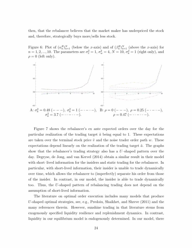
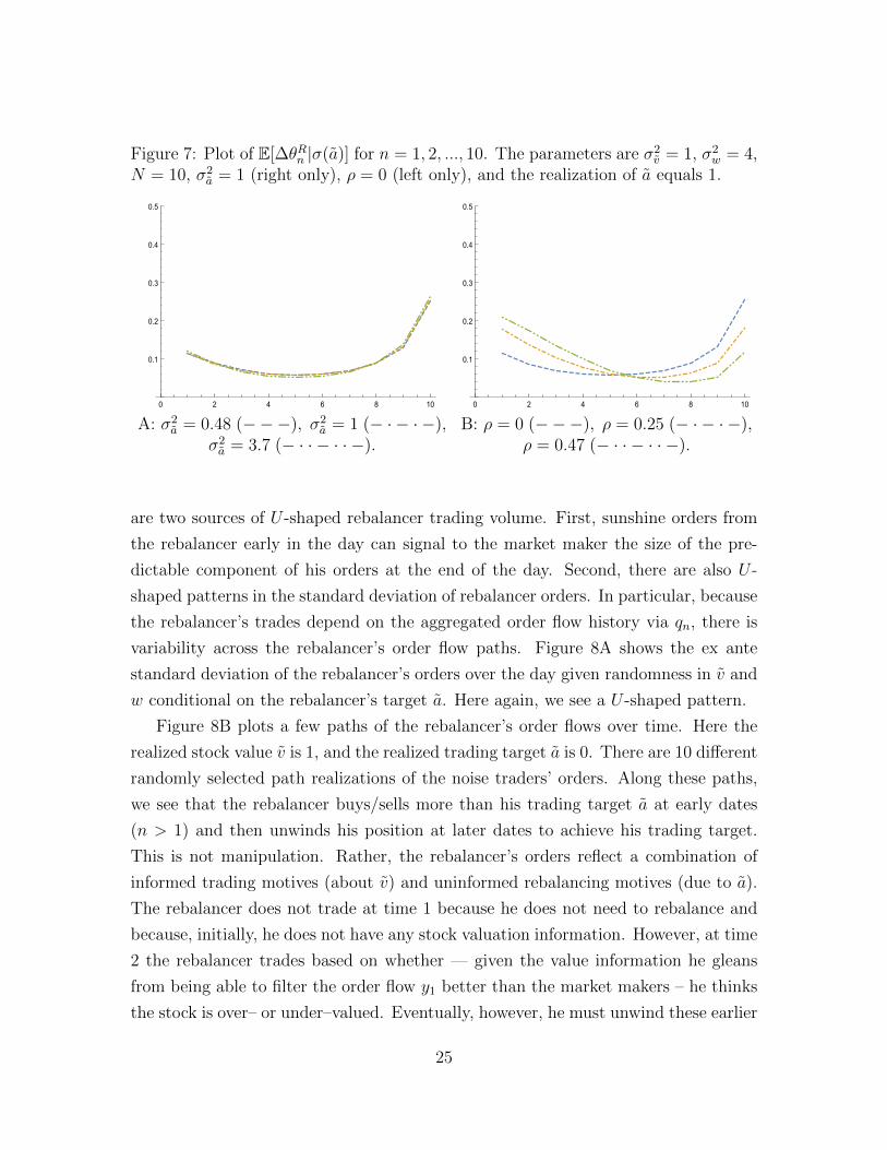
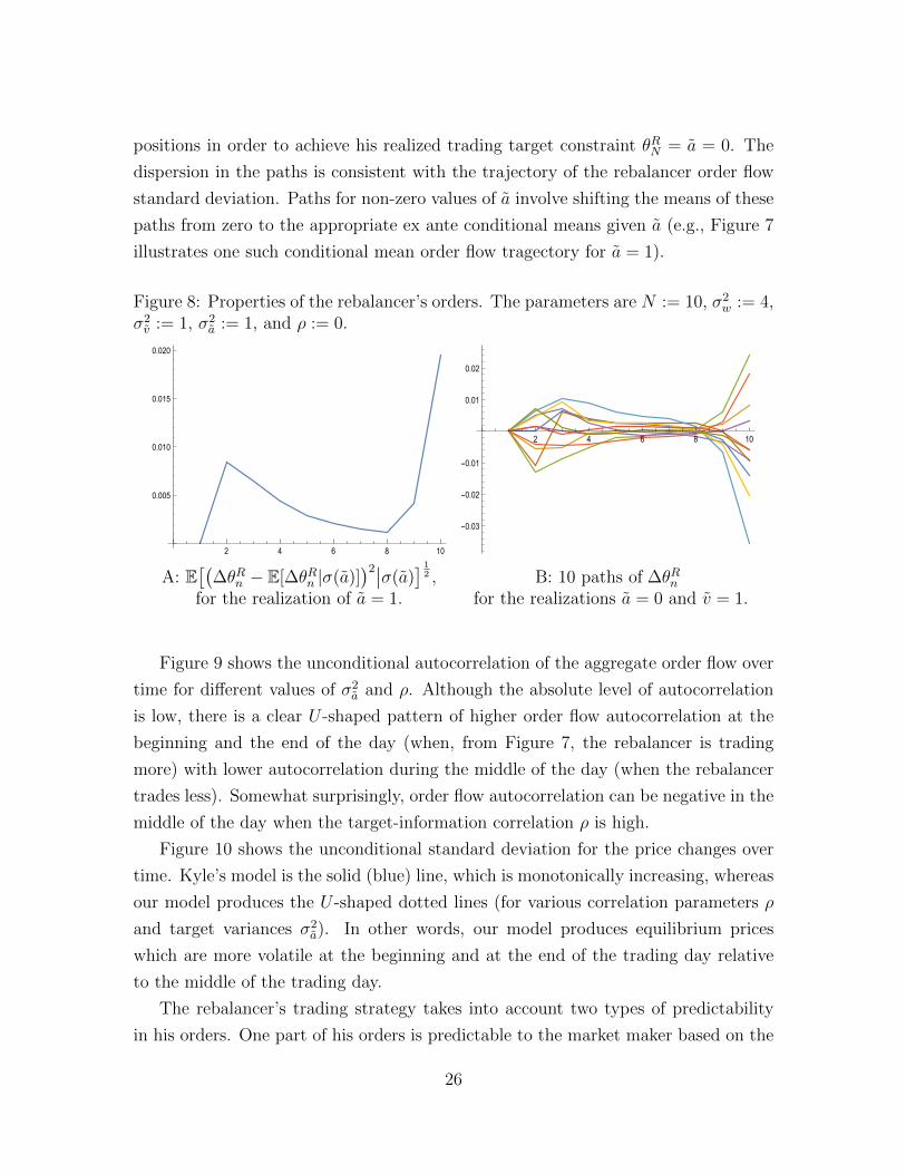
Information and Trading Targets in a Dynamic Market Equilibrium 1 Jin Hyuk Choi Department of Mathematical Sciences, Carnegie Mellon University, Pittsburgh, PA 15213, USA email: [email protected] Kasper Larsen Department of Mathematical Sciences, Carnegie Mellon University, Pittsburgh, PA 15213, USA email: [email protected] Duane J. Seppi Tepper School of Business, Carnegie Mellon University, Pittsburgh, PA 15213, USA email: [email protected] May 3, 2015 1 The authors thank Steve Shreve, Mihai Sirbu, and Gordan ˇ Zitkovi´ c for useful discussions. The second author has been supported by the National Science Foundation under Grant No. DMS- 1411809 (2014 - 2017). Any opinions, findings, and conclusions or recommendations expressed in this material are those of the authors and do not necessarily reflect the views of the National Science Foundation (NSF).
Transcript

Information and Trading Targets in a

Dynamic Market Equilibrium1

Jin Hyuk ChoiDepartment of Mathematical Sciences,

Carnegie Mellon University,

Pittsburgh, PA 15213, USA

email: [email protected]

Kasper LarsenDepartment of Mathematical Sciences,

Carnegie Mellon University,

Pittsburgh, PA 15213, USA

email: [email protected]

Duane J. SeppiTepper School of Business,

Carnegie Mellon University,

Pittsburgh, PA 15213, USA

email: [email protected]

May 3, 2015

1The authors thank Steve Shreve, Mihai Sirbu, and Gordan Zitkovic for useful discussions. Thesecond author has been supported by the National Science Foundation under Grant No. DMS-1411809 (2014 - 2017). Any opinions, findings, and conclusions or recommendations expressed inthis material are those of the authors and do not necessarily reflect the views of the National ScienceFoundation (NSF).

Information and Trading Targets in a

Dynamic Market Equilibrium

Abstract: This paper investigates the equilibrium interactions between

trading targets and private information in a multi-period Kyle (1985)

market. There are two investors who each follow dynamic trading

strategies: A strategic portfolio rebalancer who engages in order split-

ting to reach a cumulative trading target and an unconstrained strate-

gic insider who trades on long-lived information. We consider a base-

line case in which the rebalancer is initially uninformed and also cases

in which the rebalancer is initially partially informed. We derive a lin-

ear Bayesian Nash equilibrium, describe an algorithm for computing

such equilibria, and present numerical results on properties of these

equilibria.

Keywords: Market microstructure, optimal order execution, price dis-

covery, asymetric information, liquidity, portfolio rebalancing

AMS subject classifications: 93E20

JEL-Classification: G12, G11, D53

1 Introduction

Price discovery and liquidity in financial markets arise from the interactions of dif-

ferent investors with different information and trading motives using a variety of

order execution strategies.2 An important insight from Akerlof (1970), Grossman

and Stiglitz (1980), Kyle (1985), and Glosten and Milgrom (1985) is that trading

noise plays a critical role in markets subject to adverse selection when some investors

trade on superior private information. However, orders from investors with non-

informational reasons to trade also presumably reflect optimizing behavior such as

minimizing trading costs, optimizing hedging objectives, and other portfolio structur-

ing objectives. Moreover, while informed and uninformed investors trade differently,

the opportunities available to them for how to trade are presumably similar.

Our paper is the first to model optimal dynamic trading by both informed and

rebalancing investors without exogenous restrictions on information life and trading

strategies. We specifically investigate a multi-period Kyle (1985) market in which

there are two strategic investors with different trading motives who each follow opti-

mal but different dynamic trading strategies. One investor is the standard strategic

informed investor with long-lived information. The other investor is a strategic port-

folio rebalancer who can trade over multiple rounds to minimize the cost of hitting

a terminal trading target. In addition, the model has noise traders and competi-

tive market makers. In our model, the informed investor’s orders are masked by

two types of trading noise over time: Independently and identically distributed noise

trader orders and correlated randomness in the optimally chosen orders submitted by

the rebalancer with the trading target.

Our main results are:

• Sufficient conditions for a linear Bayesian Nash equilibrium are characterized

for this market.

• An algorithm for computing such equilibria numerically is provided.

• The presence of the rebalancer introduces several new features: i) the aggregate

order flow is autocorrelated, ii) expected trading for the insider and rebalancer

is U -shaped over time, and iii) the price impact of the order flow is S-shaped

2The heterogeneity of the investing public is an important fact underlying current debates abouthigh frequency trading (SEC 2010).

1

with initial price impacts above those in Kyle and later price impacts below

Kyle’s.

• The rebalancer’s trading is driven by the rebalancing target, minimizing trading

costs to reach the trading target, and profiting from any private information

he acquires endogenously over time through the trading process. As a result,

the rebalancer sometimes buys/sells more than his ultimate target and then

partially unwinds his position at the end to achieve his trading target.

Our analysis integrates two literatures on pricing and trading. The first is research

on price discovery. Kyle (1985) described equilibrium pricing and dynamic trading in a

market with noise traders and a single investor who has long-lived private information.

Subsequent work by Holden and Subrahmanyam (1992), Foster and Viswanathan

(1996), and Back, Cao, and Willard (2000) extended the model to allow for multiple

informed investors with long-lived information.

A second literature studies optimal dynamic order execution for uninformed in-

vestors with trading targets. This work includes Bertsimas and Low (1998), Almgren

and Chriss (1999, 2000), Gatheral and Scheid (2011), Engel, Ferstenberg, and Russell

(2012) and Predoiu, Shaikhet, and Shreve (2011) on optimal dynamic order execution

with trading targets and Bunnermeier and Pedersen (2005) on predatory trading in

response to predictable uninformed trading. This research all takes the price impact

function for orders as exogenous. In contrast, we model optimal order execution in

an equilibrium setting that endogenizes the price impact of orders and that reflects,

in particular, the impact of strategic uninformed trading on price impacts.3

Models combining both informed trading and optimized rebalancing have largely

been restricted to static settings or to multi-period settings with short-lived infor-

mation and/or exogenous restrictions on the rebalancer’s trading strategies. Admati

and Pfleider (1988) study a dynamic market consisting of a series of repeating one-

period trading rounds with short-lived information and uninformed liquidity traders

who only trade once but decide when to time their trading. An exception is Seppi

(1990) who models an informed investor and an uninformed strategic investor with a

trading target in a market in which both can trade dynamically. His model is solved

3In our model, order flow has a price impact due to adverse selection because of the insider’s pri-vate information. Alternatively, one could model price impacts due to inventory costs and imperfectcompetition in liquidity provision.

2

for separating and partial pooling equilibria with upstairs block trading, but only for

a restricted set of particular model parameterizations.

Our paper is related to Degryse, de Jong, and van Kervel (DJK 2014). Both their

paper and our analysis model dynamic order splitting by an uninformed investor in

a multi-period market. However, the informed investors in DJK have short-lived pri-

vate information (i.e., they only have one chance to trade on high-frequency value

innovations before they become public) whereas our insider can trade on long-lived

information over multiple intra-day time periods. Both papers have autocorrelated

(predictable) order flows because of the dynamic rebalancing. Order flow autocorrela-

tion is empirically significant but absent in previous Kyle models.4 However, there are

several notable differences between our work and DJK. First, we show that the zero

price impact of predictable orders is robust to dynamic informed trading. Thus, our

rebalancer engages in “sunshine trading,” using early trading to signal later trading.

However, the numerical magnitude of “sunshine trading” is smaller in our setting

than in DJK. This is because our informed insider can trade dynamically whereas

DJK’s series of informed traders are, by construction, unable to trade predictably

over time. Second, our analysis is possible because we use the approach of Foster and

Vishwanathan (1996) to circumvent the large state space problem mentioned in DJK.

This means that our rebalancer’s orders depend dynamically on the realized path of

aggregate orders as well as on their rebalancing target. In contrast, the rebalancer

in DJK trades deterministically over time. Third, the insider’s and the rebalancer’s

orders interact in our model. In particular, the rebalancer can learn about the in-

sider’s information, and the insider can identify and benefit from mechanical price

pressure from the rebalancer’s orders. Fourth, we derive intertemporal price impacts

and order flow patterns that differ from those in both Kyle and in DJK.

2 Model

We model a multi-period discrete-time market for a risky stock. A trading day is

normalized to the interval [0, 1] during which there are N ∈ N time points at which

trade can occur where ∆ := 1N> 0 is the time step. As in Kyle (1985), the stock’s

true value v becomes publicly known at time N + 1 after the market closes at the

4For empirical evidence on order flow autocorrelation, see Hasbrouck (1991a,b) and also therelated empirical references in Degryse, de Jong, and van Kervel (2014).

3

end of the day. The value v is normally distributed with mean zero and variance σ2v .

Additionally, there is a money market account that pays a zero interest rate.

Four types of investors trade in our model:

1. An informed trader (who we will call the insider) knows the true stock value

v at the beginning of trading and has zero initial positions in both the stock

and the money market account. The insider is risk-neutral and maximizes the

expected value of her final wealth. The insider’s order for the stock at time n,

n = 1, ..., N , is denoted by ∆θIn where θIn is her accumulated total stock position

at time n.

2. A constrained investor needs to rebalance his portfolio by buying or selling stock

to reach a terminal trading target constraint a on his ending stock position θRNby the close of the trading day. He starts the day with zero initial positions

in both the stock and the money market account.5 The target a is jointly

normally distributed with v. The variable a has zero-mean and variance σ2a and

a correlation ρ ∈ [0, 1] with the stock value v. When ρ is 0, the rebalancer is

initially uninformed. However, if ρ > 0, then we can think of the rebalancer as

being initially informed about v but subject to random binding risk limits.6 The

rebalancer is risk-neutral and maximizes the expected value of his final wealth

subject to the terminal stock position constraint. The rebalancer’s order for

the stock at time n, n = 1, ..., N , is ∆θRn , and the terminal constraint requires

∆θRN = a− θRN−1 at time N .

3. Noise traders submit net orders for stock at times n, n = 1, ..., N , that are

exogenously given by Brownian motion increments ∆wn. These increments are

normally distributed with zero-mean and variance V[∆wn] = σ2w∆ for a constant

σw > 0. We assume that w is independent of v and a.

4. Competitive risk-neutral market makers observe the aggregate net order flow

yn at times n, n = 1, ..., N , where

yn := ∆θIn + ∆θRn + ∆wn, y0 := 0. (2.1)

5Both the insider and the rebalancer finance their stock trading by borrowing/lending. Thisassumption simplifies the notation for their objective functions but is without loss of generality.

6The fact that the terminal value v is measured in dollars while the trading target a is measuredin shares is not problematic for v and a being correlated random variables.

4

Given competition and risk-neutrality, market makers clear the market (i.e.,

trade −yn) at a stock price pn set to be

pn := E[v|σ(y1, ..., yn)], n = 1, 2, ..., N, p0 := 0, (2.2)

where σ(y1, ..., yn) is the sigma-algebra generated by the order flow history.

The constrained rebalancer’s presence is the main difference between our setting

and Kyle (1985) as well as the multi-agent settings in Holden and Subrahmanyam

(1992) and Foster and Viswanathan (1996). As we shall see, the rebalancer’s presence

produces new stylized features, such as autocorrelated order flow, relative to the

existing models.

Because all initial positions are assumed to be zero (i.e., θI0 = θR0 = 0), the insider

chooses orders ∆θIn ∈ σ(v, y1, ..., yn−1) at times n, n = 1, 2, ..., N, to maximize

E[θIN(v − pN) + θIN−1∆pN + ...+ θI1∆p2

∣∣∣σ(v)]

= E

[N∑n=1

(v − pn)∆θIn

∣∣∣σ(v)

]. (2.3)

On the other hand, the rebalancer faces the terminal constraint θRN = a. Therefore,

he submits orders ∆θRn ∈ σ(a, y1, ..., yn−1) at times n, n = 1, 2, ..., N − 1, to maximize

E[a(v − pN) + θRN−1∆pN + ...+ θR1 ∆p2

∣∣∣σ(a)]

=ρσvσa

a2 − E

[N∑n=1

(a− θRn−1)∆pn

∣∣∣σ(a)

],

(2.4)

given the trading target constraint θRN = a. Here the equality follows from pN =∑Nn=1 ∆pn, p0 = 0, and E[v|σ(a)] = ρσv

σaa. As proven in the appendix, the insider’s

problem (2.3) and the rebalancer’s problem (2.4) are both quadratic optimization

problems.

Definition 2.1. A Baysian Nash equilibrium is a collection of random variables

{θIn, θRn , pn} such that

(i) given {θRn , pn}, the strategy θIn solves the insider’s problem (2.3):

max∆θIk∈σ(v,y1,...,yk−1)

1≤k≤N

E[ N∑k=1

(v − pk)∆θIk∣∣∣σ(v)

], (2.5)

5

(ii) given {θIn, pn}, the strategy θRn solves the rebalancer’s problem (2.4):

max∆θRk∈σ(v,y1,...,yk−1)

1≤k≤N−1, θRN=a

−E[ N∑k=1

(a− θRk−1)∆pk

∣∣∣σ(a)], (2.6)

(iii) given {θIn, θRn }, the pricing rule pn satisfies (2.2).

To clarify this definition, we recall the Doob-Dynkin lemma: For any random

variable B and any σ(B)-measurable random variable A we can find a deterministic

function f such that A = f(B). Therefore, we can write θRn = fRn (a, y1, . . . , yn−1),

θIn = f In(v, y1, . . . , yn), and pn = fpn(y1, . . . , yn) for three deterministic functions fRn ,

f In, and fpn. In (i), (ii), and (iii) we then mean that the functions fRn , f In, and fpn are

fixed whereas the random variables y1, ..., yn vary with the controls θI and θR.

In what follows, our goal is to construct a linear Bayesian Nash equilibrium in

which (i) the insider’s and rebalancer’s trading strategies take the forms:

∆θRn = βRn

(a− θRn−1

)+ αRn qn−1, θR0 = 0, (2.7)

∆θIn = βIn

(v − pn−1

)+ αInqn−1, θI0 = 0, (2.8)

where βRn , βIn, α

Rn , α

In, n = 1, 2, ..., N , are constants with βRN = 1 and αRN = 0, and (ii)

the pricing rule has the dynamics

∆pn = λnyn + µnqn−1, p0 := 0, (2.9)

where λn, µn are constants, and (iii) where the process qn has the dynamics

∆qn = rnyn + snqn−1, q0 := 0, (2.10)

for constants rn and sn, n = 1, 2, ..., N . The rebalancer and insider are not restricted

to use linear strategies like (2.7) and (2.8). However, we will prove that they optimally

choose such strategies in the equilibrium we construct.

The rebalancer’s trading target necessitates the introduction of the process qn

which is our model’s main new feature. Much like pn is a state variable giving the

market maker beliefs about the stock valuation, qn is a state variable indicating market

maker beliefs about the rebalancer’s remaining trading given the prior trading history.

6

There are two things to note about qn. First, the rebalancer’s trading is not limited

to be a deterministic function of his target a. Rather, his trades can also depend

on the realized prior order flow history as reflected in qn. This is in contrast to the

deterministic rebalancer trades in Degryse, de Jong, and van Kervel (2014). Second,

if equations (2.7) through (2.10) define a linear Bayesian Nash equilibrium, then

the same equilibrium (with the same prices and orders) is obtained if rn and sn are

replaced with xrn and xsn and µn, αLn , and αIn are replaced with µn/x, αRn /x, and

αIn/x for any scaler x > 0. Thus, in the equilibrium considered below, we normalize

rn and sn so that qn is the market makers’ expectation of the rebalancer’s remaining

demand a− θRn at time n based on the observed history of aggregate orders7

qn = E[a− θRn |σ(y1, ..., yn)], n = 1, ..., N. (2.11)

The term a − θRn−1 in (2.7) plays two roles in the rebalancer’s strategy. It is the

distance between the rebalancer’s current position and his final trading target a, and,

in equilibrium, it is also private information about possible misvaluation of the stock

value v − pn−1:

E[v − pn−1|σ(a, y1, ..., yn−1)] = E[v − pn−1|σ(a− θRn−1 − qn−1, y1, ..., yn−1)]

= E[v − pn−1|σ(a− θRn−1 − qn−1)].(2.12)

The first equality follows from qn−1 ∈ σ(y1, ..., yn−1) and θRn−1 ∈ σ(a, y1, ..., yn−1). The

second equality follows from the independence between v − pn−1 and y1, ..., yn−1 as

well as the independence between a − θRn−1 − qn−1 and y1, ..., yn−1. Thus, a is, in

general, incrementally informative about v beyond the past order flow history. In

particular, it is informative at n > 1 even if ρ = 0.

Similarly, the term v − pn−1 in (2.8) plays two roles in the insider’s strategy. It

is both private information about the stock value and, in equilibrium, informative

about the remaining demand a− θRn−1 for the rebalancer:

E[a− θRn−1|σ(v, y1, ..., yn−1)]

= qn−1 + E[a− θRn−1 − qn−1|σ(v − pn−1, y1, ..., yn−1)]

= qn−1 + E[a− θRn−1 − qn−1|σ(v − pn−1)].

(2.13)

7An alternative scaling would be to set qn−1 equal to E[yn|σ(y1, ..., yn−1)].

7

The first equality follows from qn−1, pn−1 ∈ σ(y1, ..., yn−1). The second equality follows

from the independence between v − pn−1 and y1, ..., yn−1 as well as the independence

between a− θRn−1 − qn−1 and y1, ..., yn−1.

2.1 Equilibrium

In this section we characterize sufficient conditions for existence of a linear Bayesian

Nash equilibrium of the form in (2.7) through (2.10). The characterization follows

the logic of Foster and Viswanathan (1996) closely. Figure 1 graphically illustrates

the steps we use to describe sufficient equilibrium conditions.

 Set  of  possible  coefficients   Set  of  “hat”  processes  

Set  of  Kalman  filter  coefficients  

Set  of  FOC  coefficients  

Fixed  point  requirement  for  a  linear  Bayesian  Nash  equilibrium  

Figure 1: Venn diagrams illustrating the various constants entering the fixed pointwhich describes the Baysian Nash equilibrium.

To begin, we consider the complete set of all possible candidate values for the

equilibrium constants

λn, µn, rn, sn, βRn , α

Rn , β

In, α

In, n = 1, . . . , N, (2.14)

8

with

βRN = 1, αRN = 0. (2.15)

The restrictions in (2.15) at date N reflect the fact that the rebalancer must achieve

his target a after his last round of trade. Our goal is to identify sufficient conditions

for a candidate set of specific coefficient values to be an equilibrium. We do this in

three steps.

The first step takes a set of candidate constants (2.14)-(2.15) and computes (us-

ing the terminology and notation of Foster and Viswanathan 1996) a corresponding

system of “hat” price and order flow processes

∆θIn = βIn(v − pn−1) + αInqn−1, θI0 := 0, (2.16)

∆θRn = βRn (a− θRn−1) + αRn qn−1, θR0 := 0, (2.17)

yn = ∆θIn + ∆θRn + ∆wn, (2.18)

∆pn = λnyn + µnqn−1, p0 := 0, (2.19)

∆qn = rnyn + snqn−1, q0 := 0. (2.20)

The system of processes (∆pn,∆qn, yn,∆θIn,∆θ

Rn ) is fully specified (autonomous) by

the coefficients (2.14)-(2.15). Furthermore, given the zero-mean and joint normality

of v, a, and w, the “hat” system is also zero-mean and jointly normal. We define the

variances and covariance for the “hat” dynamics, n = 2, ..., N , by

Σ(1)n := V

[a− θRn−1 − qn−1

], (2.21)

Σ(2)n := V[v − pn−1

], (2.22)

Σ(3)n := E

[(a− θRn−1 − qn−1

)(v − pn−1)

], (2.23)

where the initial variances and covariance at n = 1 are

Σ(1)1 = σ2

a, Σ(2)1 = σ2

v , Σ(3)1 = ρ. (2.24)

The “hat” processes will be used to make (2.3) and (2.4) analytically tractable

in the sense that both the insider’s problem and the rebalancer’s problem can be de-

scribed by a five-dimensional state process; see (2.34) and (2.37) below. In particular,

9

the “hat” processes denote the processes that agents believe other agents believe de-

scribe the equilibrium. In equilibrium, these beliefs must be correct. This consistency

requirement imposes two groups of conditions that a set of candidate constants must

satisfy to be equilibrium constants. The next two steps explain these conditions.

The second step requires the coefficients, λn, µn, sn, and rn, of the price and order

flow state variable processes to be consistent in equilibrium with Bayesian updating.

In particular, if market makers believe that the insider and rebalancer are following

the “hat” strategies, then we can re-write (2.2) as

∆pn = λn(yn − E[yn|σ(y1, ..., yn−1)]

)= λn

(yn − [βRn E[a− θRn−1|σ(y1, ..., yn−1)] + αRn qn−1 + αInqn−1]

)= λn

(yn − (αIn + αRn + βRn )qn−1

),

(2.25)

for n = 1, ..., N . The first equality follows from the fact that, given the jointly Gaus-

sian structure of the “hat” processes, conditional expectations are linear projections.

The second equality follows from (i) the definition of the aggregate order flow, (ii)

the fact that v − pn−1 is independent of past order flows, and (iii) the assumption

that the noise trader orders are zero–mean and i.i.d. over time. The final equality

follows from the assumption that in our conjectured equilibrium pn is linear in qn−1

and the normalization that qn−1 = E[a− θRn−1|σ(y1, ..., yn−1)]. Comparing the last line

of (2.25) with (2.9) and using the fact that λn equals the projection coefficient

Cov(v − pn−1, yn − E[yn|σ(y1, ..., yn−1)])

V(yn − E[yn|σ(y1, ..., yn−1)])(2.26)

gives restrictions on the coefficients of the price process in terms of the insider and

rebalancer strategy coefficients. A similar logic can also be used to derive restrictions

on the coefficients of the qn process in terms of the investor strategy coefficients.

Thus, these calculations lead to four restrictions on the state–variable and strategy

constants in a linear Bayesian Nash equilibrium for n = 1, ..., N :

10

Condition 2.2. In equilibrium, the price and order flow state variable coefficients

depend on the insider and rebalancer order coefficients as follow:

λn =βInΣ

(2)n + βRn Σ

(3)n

(βIn)2Σ(2)n + (βRn )2Σ

(1)n + 2βInβ

Rn Σ

(3)n + σ2

w∆, (2.27)

rn =(1− βRn )(βInΣ

(3)n + βRn Σ

(1)n )

(βIn)2Σ(2)n + (βRn )2Σ

(1)n + 2βInβ

Rn Σ

(3)n + σ2

w∆, (2.28)

µn = −(αIn + αRn + βRn )λn, (2.29)

sn = −(αIn + αRn + βRn )rn − (αRn + βRn ), (2.30)

where the conditional variances and covariance from (2.21)-(2.23) can now be explic-

itly specified as (see the proof of Lemma A.1 in Appendix A.1)

Σ(1)n = (1− βRn−1)

((1− βRn−1 − rn−1β

Rn−1)Σ

(1)n−1 − rn−1β

In−1Σ

(3)n−1

), (2.31)

Σ(2)n = (1− λn−1β

In−1)Σ

(2)n−1 − λn−1β

Rn−1Σ

(3)n−1, (2.32)

Σ(3)n = (1− βRn−1)

((1− λn−1β

In−1)Σ

(3)n−1 − λn−1β

Rn−1Σ

(1)n−1

). (2.33)

Note that Condition 2.2 has a “block” structure. The variances and covariance

Σ(1)n , Σ

(2)n , and Σ

(3)n at time n just depend on prior coefficients and prior variances

and covariance from time n− 1. The values of λn and rn just depend on the βRn and

βIn strategy coefficients and the variances and covariance at time n (along with the

exogenous noise trading variance σ2w). Lastly, µn and sn depend on λn and µn and

the full set of strategy coefficients at time n.

The third step begins by deriving value functions for the optimization problems

for the two strategic investors. Consider first the insider at a generic time n. Given

her trades ∆θI1, . . . ,∆θIn — which need not be consistent with the candidate “hat”

dynamics — the insider not only knows the final stock value v, but also the extent to

which the actual prices and rebalancer’s order flow at date n deviate from the values

they would have had if she had instead traded as in the candidate “hat” processes.

Thus, the state variables at date n for the insider’s value function are

X(1)n := v − pn, X(2)

n := qn, X(3)n := θRn − θRn , X(4)

n := qn − qn, X(5)n := pn − pn. (2.34)

11

Here the “un-hatted” variables are the variable values given her actual (potentially

arbitrary) orders, see (2.9) and (2.10), whereas the “hat” variables are not affected

by actual orders. When the rebalancer’s strategy is taken to be fixed by (2.7), it is

characterized by the two sequences of candidate constants βR1 , . . . , βRN and αR1 , . . . , α

RN .

However, even though the rebalancer’s strategy is fixed, its realizations are subject to

the insider’s choice of control θI since the aggregate order flow affects the rebalancer’s

actual orders. Thus, the state variable X(3)n measures the effect of the insider’s actual

orders on the rebalancer’s actual orders. A similar interpretation applies to X(4)n and

X(5)n and the order flow state variable qn and prices pn. In equilibrium, we will see

that the three deviation state variables X(3), X(4), and X(5) are zero. However, in

deriving the equilibrium, we need to allow for the possibility of past suboptimal play.

We show (see the appendix) that the insider’s value function for n = 0, 1, ..., N

has a quadratic form

max∆θIk∈σ(v,y1,...,yk−1)

n+1≤k≤N

E[ N∑k=n+1

(v − pk)∆θIk∣∣∣σ(v, y1, ..., yn)

]= I(0)

n +∑

1≤i≤j≤5

I(i,j)n X(i)

n X(j)n ,

(2.35)

where I(0)n and I

(i,j)n are coefficients computed recursively from the candidate coef-

ficients (2.14)-(2.15). We use the Bellman principle to derive the value function

coefficients at time n (i.e., I(0)n and I

(i,j)n ) in terms of the value function coefficients at

time n + 1, which, in turn, depend on the strategy and pricing coefficients at times

n+ 1, . . . , N . The next section describes this recursion in detail.

Similarly, when the insider’s strategy is given by (2.8), an analogous argument

can be used to derive a quadratic value function for the rebalancer

max∆θRk∈σ(a,y1,...,yk−1)

n+1≤k≤N−1

−E[ N∑k=n+1

(a− θRk−1)∆pk

∣∣∣σ(a, y1, ..., yn)]

= L(0)n +

∑1≤i≤j≤5

L(i,j)n Y (i)

n Y (j)n .

(2.36)

Here the state variables are

Y (1)n := a− θRn , Y (2)

n := qn, Y(3)n := θRn − θRn , Y (4)

n := qn − qn, Y (5)n := pn − pn, (2.37)

12

given a prior sequence of (potentially off-equilibrium) trades ∆θR1 , . . . ,∆θRn . The co-

efficients L(0)n and L

(i,j)n are again computed recursively from the candidate coefficients

(2.14) and (2.15). In equilibrium, the deviation state variables Y (3), Y (4), and Y (5)

are again zero.

The first– and second–order conditions for the insider’s and rebalancer’s max-

imization problems, given the insider’s and rebalancer’s value functions, lead to a

group of equilibrium restrictions on the investor strategy coefficients βIn, βRn , αIn, and

αRn in terms of the price and order flow state variable coefficients.

Condition 2.3. Given the conditional variances Σ(1)N and Σ

(2)N and covariance Σ

(3)N at

time N from (2.21)-(2.23), the candidate constants satisfy (recall that βRN = 1)

βIN =( 1

2λN− Σ

(3)N

2Σ(2)N

), λN > 0. (2.38)

In addition, for n = 1, . . . , N − 1, given the variances and covariance Σ(1)n ,Σ

(2)n , Σ

(3)n ,

the candidate coefficients in (2.14)-(2.15) solve the following four polynomial equa-

tions:

2λnβIn = −(rnI

(1,4)n + λnI

(1,5)n )

(1− λn(βIn +

βRn Σ(3)n

Σ(2)n

))

− (rnI(2,4)n + λnI

(2,5)n )rn(βIn +

βRn Σ(3)n

Σ(2)n

) + 1− λnβRn Σ

(3)n

Σ(2)n

, (2.39)

0 = λn + (1− βRn )(L(1,3)n + rnL

(1,4)n + λnL

(1,5)n

)+ rn

(βRn +

βInΣ(3)n

Σ(1)n

)(L(2,3)n + rnL

(2,4)n + λnL

(2,5)n

), (2.40)

αRn = −

(L

(2,3)n + rnL

(2,4)n + λnL

(2,5)n

)(rnβ

Rn + rn

βInΣ(3)n

Σ(1)n

+ βRn − 1)

L(1,3)n + rnL

(1,4)n + λnL

(1,5)n + L

(2,3)n + rnL

(2,4)n + λnL

(2,5)n

, (2.41)

αIn =(rnI

(2,4)n + λnI

(2,5)n )(αRn + βRn − 1)

λn, (2.42)

where the I and L terms are from the two investor value functions (2.35) and (2.36).

The candidate constants and the value function terms must also satisfy the two in-

13

equalities:

− λn + I(4,5)n λnrn + I(4,4)

n r2n + I(5,5)

n λ2n < 0, (2.43)

L(3,3)n + L(3,4)

n rn + L(3,5)n λn + L(4,4)

n r2n + L(5,5)

n λ2n + L(4,5)

n rnλn < 0, (2.44)

which (as we show in the appendix) ensure sufficiency of the first-order-conditions.

♦Here again, the equilibrium restrictions have a “block” structure in that αIn and

αRn in (2.41) and (2.42) depend on βIn and βRn , whereas the linear equations (2.39) and

(2.40) – which are the first-order conditions for the insider and rebalancer at date n

– can be solved to express βIn and βRn in terms of the current updating coefficients

and value function coefficients (which only depend on the updating and strategy

coefficients at later dates) but not on αIn and αRn .

Our main theoretical result is the following:

Theorem 2.4. If the constants (2.14) and (2.15) satisfy Conditions 2.2 and 2.3, then

a linear Bayesian Nash equilibrium exists of the form given in equations (2.7)-(2.10).

Furthermore, we have

αIn = I(1,2)n = I(2,2)

n = I(2,3)n = I(2,4)

n = I(2,5)n = 0 for n = 1, 2, ..., N,

rN = 0, µN = −λN , sN = −1.(2.45)

The new feature in our model, compared to Foster and Viswanathan (1996) and

Kyle (1985), is the presence of the qn process in the equilibrium price dynamics

(2.9). This produces new stylized features including autocorrelation of the equilibrium

aggregate order flow:

E[yn|σ(y1, ..., yn−1)]

= E[∆θIn + ∆θRn + ∆wn|σ(y1, ..., yn−1)]

= αRn qn−1 + E[βIn(v − pn−1) + βRn (a− θRn−1)|σ(y1, ..., yn−1)]

= (αRn + βRn ) qn−1,

(2.46)

which, in general, is not zero. The second equality uses the fact from Theorem 2.4

that αIn = 0. The last equality follows, in part, from the earlier observation that,

in equilibrium qn−1 is the conditional expectation of a− θRn−1 given the prior trading

14

history.

2.2 Algorithm

This section describes an algorithm for searching numerically for a linear Bayesian

Nash equilibrium. The algorithm is similar in logic to the algorithm in Section V in

Foster and Viswanathan (1996), except that our algorithm requires three constants as

inputs (due to the presence of two strategic agents) whereas Foster and Viswanathan

(1996) only requires one constant as an input.

To describe the algorithm we assume that the conclusions of Lemma A.2 and

Lemma A.4 (see the appendix) are valid. The algorithm starts by taking as inputs

three conjectured constants:

Σ(1)N > 0, Σ

(2)N > 0, Σ

(3)N ∈ R such that

(3)N

)2 ≤ Σ(1)N Σ

(2)N , (2.47)

and proceeds through backward induction.8

Starting step for time N : We need λN and βIN to satisfy (2.27) for n = N and

(2.38). Given those two constants, we can define the constants

βRN := 1, αRN := αIN := rN := 0, µN := −λN , sN := −1. (2.48)

Based on Lemma A.2 and Lemma A.4 we can then let I(0)N−1, I

(i,j)N−1, L

(0)N−1, and L

(i,j)N−1,

1 ≤ i ≤ j ≤ 5, be the coefficients appearing in the two representations:

max∆θIN

E[(v − pN)∆θIN

∣∣∣σ(v, y1, ..., yN−1)]

= I(0)N−1 +

∑1≤i≤j≤5

I(i,j)N−1X

(i)N−1X

(j)N−1, (2.49)

E[− (a− θRN−1)∆pN

∣∣∣σ(a, y1, ..., yN−1)]

= L(0)N−1 +

∑1≤i≤j≤5

L(i,j)N−1Y

(i)N−1Y

(j)N−1. (2.50)

Induction step: At each time n the algorithm takes the following constants as input:

Σ(1)n+1,Σ

(2)n+1,Σ

(3)n+1, I

(0)n , (I(i,j)

n )1≤i≤j≤5, L(0)n , (L(i,j)

n )1≤i≤j≤5. (2.51)

Given these constants, (λn, rn, βIn, β

Rn ,Σ

(1)n ,Σ

(2)n ,Σ

(3)n ) must satisfy (2.27)-(2.28), (2.39)-

(2.40), and (2.31)-(2.33). This gives a system of seven polynomial equations in

8Σ(2) must be non-increasing over time (as in Kyle 1985) but Σ(1) might not be.

15

seven unknown constants. Given a solution to these seven equations, we obtain

(µn, sn, αIn, α

Rn ) from (2.29), (2.30), (2.41), and (2.42).

Next, to compute the coefficients in the value functions at time n− 1; that is,

I(0)n−1, (I

(i,j)n−1)1≤i≤j≤5, L

(0)n−1, (L

(i,j)n−1)1≤i≤j≤5, (2.52)

we consider the following two optimization problems:

max∆θIn

E[(v − pn)∆θIn + I(0)

n +∑

1≤i≤j≤5

I(i,j)n X(i)

n X(j)n

∣∣∣σ(v, y1, ..., yn−1)], (2.53)

max∆θRn

E[− (a− θRn−1)∆pn + L(0)

n +∑

1≤i≤j≤5

L(i,j)n Y (i)

n Y (j)n

∣∣∣σ(a, y1, ..., yn−1)]. (2.54)

According to Lemma A.2, the insider’s problem (2.53) is quadratic in ∆θIn whereas

Lemma A.4 ensures that the rebalancer’s problem (2.54) is quadratic in ∆θRn . The

first-order-condition produces the candidate optimizer for the insider’s order ∆θIn

5∑i=1

γ(i)n X

(i)n−1, n = 1, ..., N, (2.55)

16

where

γ(1)n := 1

2(λn−I(4,5)

n λnrn−I(4,4)n r2

n−I(5,5)n λ2

n

)(− (rnI(1,4)n + λnI

(1,5)n )

(1− λn(βIn +

βRn Σ(3)n

Σ(2)n

))

− (rnI(2,4)n + λnI

(2,5)n )rn(βIn +

βRn Σ(3)n

Σ(2)n

) (2.56)

− 2βIn(λnrnI

(4,5)n + r2

nI(4,4)n + λ2

nI(5,5)n

)+ 1− λnβ

Rn Σ

(3)n

Σ(2)n

),

γ(2)n := 1

2(λn−I(4,5)

n λnrn−I(4,4)n r2

n−I(5,5)n λ2

n

)((rnI(1,4)n + λnI

(1,5)n )

(λn(αIn + αRn + βRn ) + µn

)− (rnI

(2,4)n + λnI

(2,5)n )

(1 + rn(αIn + αRn + βRn ) + sn

)(2.57)

− 2αIn(λnrnI

(4,5)n + r2

nI(4,4)n + λ2

nI(5,5)n

)−(λn(αRn + βRn ) + µn

)),

γ(3)n :=

−(rnI(3,4)n +λnI

(3,5)n )(1−βRn )+2βRn

(λnrnI

(4,5)n +r2

nI(4,4)n +λ2

nI(5,5)n

)−λnβRn

2(λn−I(4,5)

n λnrn−I(4,4)n r2

n−I(5,5)n λ2

n

) , (2.58)

γ(4)n := 1

2(λn−I(4,5)

n λnrn−I(4,4)n r2

n−I(5,5)n λ2

n

)(− (rnI(3,4)n + λnI

(3,5)n )αRn

− 2(λnrnI

(4,5)n + r2

nI(4,4)n + λ2

nI(5,5)n

)αRn − I(4,5)

n (λn(sn + 1) + rnµn) (2.59)

− 2rnI(4,4)n (sn + 1)− 2λnI

(5,5)n µn + (λnα

Rn + µn)

),

γ(5)n := 1−I(4,5)

n rn−2λnI(5,5)n

2(λn−I(4,5)

n λnrn−I(4,4)n r2

n−I(5,5)n λ2

n

) . (2.60)

Furthermore, the second-order condition (2.43) ensures that this candidate optimizer

indeed maximizes the insider’s objective. As an aside, we note that (2.39) and (2.42)

come from (2.56) and (2.57) when the equilibrium conditions γ(1)n = βIn and γ

(2)n = αIn

are imposed.

Similarly, the candidate optimizer for the rebalancer’s order ∆θRn at time n is

5∑i=1

δ(i)n Y

(i)n−1, n = 1, ..., N, (2.61)

17

where

δ(1)n := 1

2(L

(3,3)n +L

(3,4)n rn+L

(3,5)n λn+L

(4,4)n r2

n+L(5,5)n λ2

n+L(4,5)n rnλn

)×(λn + (1− βRn )

(L(1,3)n + rnL

(1,4)n + λnL

(1,5)n

)+ rn

(βRn +

βInΣ(3)n

Σ(1)n

)(L(2,3)n + rnL

(2,4)n + λnL

(2,5)n

)+ 2βRn

(L(3,3)n + L(3,4)

n rn + L(3,5)n λn + L(4,4)

n r2n + L(5,5)

n λ2n + L(4,5)

n rnλn)),

(2.62)

δ(2)n := − 1

2(L

(3,3)n +L

(3,4)n rn+L

(3,5)n λn+L

(4,4)n r2

n+L(5,5)n λ2

n+L(4,5)n rnλn

)×(αRn(L(1,3)n + rnL

(1,4)n + λnL

(1,5)n

)−(rn(αIn + αRn −

βInΣ(3)n

Σ(1)n

) + sn + 1)(L(2,3)n + rnL

(2,4)n + λnL

(2,5)n

)− 2αRn

(L(3,3)n + L(3,4)

n rn + L(3,5)n λn + L(4,4)

n r2n + L(5,5)

n λ2n + L(4,5)

n rnλn)),

(2.63)

δ(3)n := λn+2L

(3,3)n +L

(3,4)n rn+L

(3,5)n λn

2(L

(3,3)n +L

(3,4)n rn+L

(3,5)n λn+L

(4,4)n r2

n+L(5,5)n λ2

n+L(4,5)n rnλn

) , (2.64)

δ(4)n := (L

(3,4)n +2L

(4,4)n rn+L

(4,5)n λn)(rnαIn+sn+1)+(L

(3,5)n +2L

(5,5)n λn+L

(4,5)n rn)(λnαIn+µn)

2(L

(3,3)n +L

(3,4)n rn+L

(3,5)n λn+L

(4,4)n r2

n+L(5,5)n λ2

n+L(4,5)n rnλn

) , (2.65)

δ(5)n := −βIn

(L

(3,4)n rn+L

(3,5)n λn+2L

(4,4)n r2

n+2L(5,5)n λ2

n+2L(4,5)n rnλn

)−L(3,5)

n −2λnL(5,5)n −rnL(4,5)

n

2(L

(3,3)n +L

(3,4)n rn+L

(3,5)n λn+L

(4,4)n r2

n+L(5,5)n λ2

n+L(4,5)n rnλn

) . (2.66)

Again, (2.44) ensures that this candidate optimizer indeed maximizes the rebalancer’s

objective. We also note that (2.40) and (2.41) come from (2.62) and (2.63) when the

equilibrium conditions δ(1)n = βRn and δ

(2)n = αRn are imposed.

The value function constants for time n−1 are then found by inserting the optimal

strategies (2.55) and (2.61) into the two problems (2.53) and (2.54) and then matching

coefficients.

Termination: The iteration above is continued back to time n = 1. If the resulting

values at n = 1 satisfy

Σ(1)1 = σ2

a, Σ(2)1 = σ2

v , Σ(3)1 = ρ, (2.67)

the algorithm terminates and the computed coefficients produce a linear Bayesian

Nash equilibrium. Otherwise, we adjust the conjectured starting input values in

(2.47) and start the algorithm all over.

18

3 Numerical results

As is common with multi-period Kyle-type models, we do not have analytic com-

parative results about the properties of our model. However, we have conducted a

variety of numerical experiments to illustrate properties of the model. The baseline

specification for our model has N = 10 rounds of trading, the variance of the terminal

stock value v is normalized to σ2v = 1, the total variance of the Brownian motion noise

trading order flow over the N periods is fixed at σ2w = 4, the variance of the trading

target a is σ2a = 1, and the correlation between the trading target a and the terminal

stock value v is ρ = 0. In our analysis, we vary the correlation ρ and the variance of

the trading target σ2a.

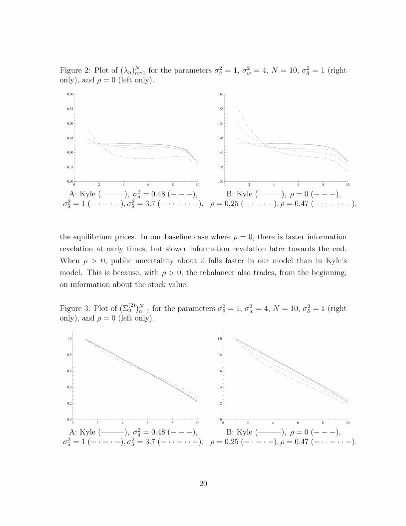
The two graphs in Figure 2 show the price impact of order flow parameter λn over

time. The various dashed lines are for different parameterizations of our model. For

comparison, the solid (blue) line is the corresponding price impact in Kyle (1985) in

which the rebalancer is absent. In the first round of trading at time n = 1, rebalancing

noise by itself would reduce the value of λ1 relative to Kyle (1985). However, in

equilibrium, the insider’s trading strategy also changes. The net effect in this example

is that λ1 increases relative to Kyle (1985).9 At later times n > 2, the price impacts

are lower than in Kyle. The result is an S-shaped twist in λn over time. The price

impact trajectory in our model also differs from Degryse, de Jong, and van Kervel

(2014) in which price impacts have an inverted U -shape (see their Figure 1).

Figure 2A varies the variance of the trading target σ2a while holding ρ fixed at 0.

We see that the S-shaped twist in λn becomes stronger for larger values of σ2a. When

σ2a is high enough, the price impact of order flow can even be non-monotone over

time (see the dashed line corresponding to σ2a = 3.7, which is comparable to the total

daily noise trader order variance σ2w = 4). Figure 2B varies the correlation ρ between

the terminal stock value v and the trading target a holding the variance σ2a fixed at

1. Here again, there is an asymmetric impact of ρ over time relative to our baseline

model with ρ = 0. At early times, λn is increasing in the correlation ρ, but at later

times, λn is decreasing in ρ. This is because increasing ρ changes some rebalancing

trades from noise into informative order flow.

Figure 3 shows the trajectory of the variance Σ(2)n of v−pn−1 over time where pn are

9From equation (2.27) we see that λn is non-monotone in the aggressiveness of informed trading.Thus, there may also be parameterizations for which our model produces an inverted U -shape forλn.

19

Figure 2: Plot of (λn)Nn=1 for the parameters σ2v = 1, σ2

w = 4, N = 10, σ2a = 1 (right

only), and ρ = 0 (left only).

0 2 4 6 8 100.30

0.35

0.40

0.45

0.50

0.55

0.60

0 2 4 6 8 100.30

0.35

0.40

0.45

0.50

0.55

0.60

A: Kyle (———), σ2a = 0.48 (−−−), B: Kyle (———), ρ = 0 (−−−),

σ2a = 1 (− · − · −), σ2

a = 3.7 (− · · − · · −). ρ = 0.25 (− · − · −), ρ = 0.47 (− · · − · · −).

the equilibrium prices. In our baseline case where ρ = 0, there is faster information

revelation at early times, but slower information revelation later towards the end.

When ρ > 0, public uncertainty about v falls faster in our model than in Kyle’s

model. This is because, with ρ > 0, the rebalancer also trades, from the beginning,

on information about the stock value.

Figure 3: Plot of (Σ(2)n )Nn=1 for the parameters σ2

v = 1, σ2w = 4, N = 10, σ2

a = 1 (rightonly), and ρ = 0 (left only).

0 2 4 6 8 100.0

0.2

0.4

0.6

0.8

1.0

0 2 4 6 8 100.0

0.2

0.4

0.6

0.8

1.0

A: Kyle (———), σ2a = 0.48 (−−−), B: Kyle (———), ρ = 0 (−−−),

σ2a = 1 (− · − · −), σ2

a = 3.7 (− · · − · · −). ρ = 0.25 (− · − · −), ρ = 0.47 (− · · − · · −).

20

Figure 4 shows the insider’s strategy coefficients βIn, which measures how aggres-

sively she trades on her private information v − pn−1 over time.10 As in Kyle, the

intensity of informed trading in our model also increases as time approaches the ter-

minal time N . This is consistent with the fact that the price impact of order flow λn

in Figure 2 shrinks as time passes. We also see that as the variance of the trading

target σ2a increases, the informed investor trades more aggressively at early dates, less

so in the middle, and then slightly more aggressively again towards the end. The

informed trader’s increased initial aggressiveness reflects the fact that there is more

noise, due to the rebalancer’s trading target a, in which to hide the insider’s orders.

In addition, if ρ > 0, insider trading aggressiveness increases somewhat due to a

Holden-Subrahmanyam race–to–trade competition effect. The apparent size of the

changes in βI1 – which are on the order of 10 percent – are visually understated in

Figure 4 because of the vertical scaling (due to the size of βI10). In the next figure,

we will see that the impact of these changes on order size is nontrivial.11

Figure 4: Plot of (βIn)Nn=1 for the parameters σ2v = 1, σ2

w = 4, N = 10, σ2a = 1 (right

only), and ρ = 0 (left only).

0 2 4 6 8 100.0

0.5

1.0

1.5

0 2 4 6 8 100.0

0.5

1.0

1.5

A: Kyle (———), σ2a = 0.48 (−−−), B: Kyle (———), ρ = 0 (−−−),

σ2a = 1 (− · − · −), σ2

a = 3.7 (− · · − · · −). ρ = 0.25 (− · − · −), ρ = 0.47 (− · · − · · −).

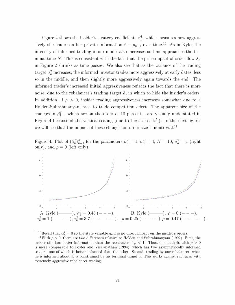
10Recall that αIn = 0 so the state variable qn has no direct impact on the insider’s orders.

11With ρ > 0, there are two differences relative to Holden and Subrahmanyam (1992). First, theinsider still has better information than the rebalancer if ρ < 1. Thus, our analysis with ρ > 0is more comparable to Foster and Viswanathan (1994), which has two asymmetrically informedtraders, one of which is better informed than the other. Second, trading by our rebalancer, whenhe is informed about v, is constrained by his terminal target a. This works against rat races withextremely aggressive rebalancer trading.

21

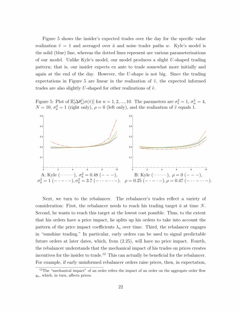
Figure 5 shows the insider’s expected trades over the day for the specific value

realization v = 1 and averaged over a and noise trader paths w. Kyle’s model is

the solid (blue) line, whereas the dotted lines represent are various parameterizations

of our model. Unlike Kyle’s model, our model produces a slight U -shaped trading

pattern; that is, our insider expects ex ante to trade somewhat more initially and

again at the end of the day. However, the U -shape is not big. Since the trading

expectations in Figure 5 are linear in the realization of v, the expected informed

trades are also slightly U -shaped for other realizations of v.

Figure 5: Plot of E[∆θIn|σ(v)] for n = 1, 2, ..., 10. The parameters are σ2v = 1, σ2

w = 4,N = 10, σ2

a = 1 (right only), ρ = 0 (left only), and the realization of v equals 1.

0 2 4 6 8 10

0.1

0.2

0.3

0.4

0.5

0 2 4 6 8 10

0.1

0.2

0.3

0.4

0.5

A: Kyle (———), σ2a = 0.48 (−−−), B: Kyle (———), ρ = 0 (−−−),

σ2a = 1 (− · − · −), σ2

a = 3.7 (− · · − · · −). ρ = 0.25 (− · − · −), ρ = 0.47 (− · · − · · −).

Next, we turn to the rebalancer. The rebalancer’s trades reflect a variety of

consideration: First, the rebalancer needs to reach his trading target a at time N .

Second, he wants to reach this target at the lowest cost possible. Thus, to the extent

that his orders have a price impact, he splits up his orders to take into account the

pattern of the price impact coefficients λn over time. Third, the rebalancer engages

in “sunshine trading.” In particular, early orders can be used to signal predictable

future orders at later dates, which, from (2.25), will have no price impact. Fourth,

the rebalancer understands that the mechanical impact of his trades on prices creates

incentives for the insider to trade.12 This can actually be beneficial for the rebalancer.

For example, if early uninformed rebalancer orders raise prices, then, in expectation,

12The “mechanical impact” of an order refers the impact of an order on the aggregate order flowyn, which, in turn, affects prices.

22

the insider should then buy less/sell more in the future, thereby putting downward

pressure on later prices which, in turn, reduces the expected cost of future rebalancer

buying. Fifth, the rebalancer trades on information about the asset value v. If

ρ > 0, the rebalancer starts out with stock valuation information. However, even

if the rebalancer is initially uninformed about v (i.e., ρ = 0), he still acquires stock

valuation information over time (see (2.12)) that he can use to reduce his rebalancing

costs and even, possibly, to earn a trading profit. In particular, he can filter the

aggregate order flow to learn about the insider’s trading, and thereby learn about v,

better than the market makers.

To gain further intuition, we rearrange (2.7) to decompose the rebalancer’s order

at time n as follows:

∆θRn =(

∆θRn − E[∆θRn |σ(y1, . . . , yn−1)])

+ E[∆θRn |σ(y1, . . . , yn−1)]

= βRn (a− θRn−1 − qn−1) + (αRn + βRn )qn−1.(3.1)

The second component, (αRn + βRn )qn−1, is the market maker’s expectation of the

rebalancer’s order at time n. This is the amount the rebalancer trades at time n

with no price impact. The first component, βRn (a − θRn−1 − qn−1), represents the

combined effect of i) strategic trading by the rebalancer on his private information,

a− θRn−1 − qn−1, which is informative about v− pn−1 (see (2.12)), and ii) rebalancing

trading given that the remaining amount that the rebalancer actually needs to trade

(i.e., a− θRn−1) differs, in general, from the market maker’s expectation qn−1.

Figure 6 shows trajectories for the rebalancer’s strategy coefficients βRn and αRn .

We use the decomposition (3.1) to interpret them. Since αRn + βRn is positive but

small until time N , the rebalancer trades a relatively small fraction of his expected

trading gap qn−1 over time until time N at which time αRN + βRN = 1 and then he

trades the full remaining gap. In addition, the fact that βRn is positive means that

the rebalancer trades in the direction of his private information. He does this for two

reasons: First, the larger a is relative to θRn−1 (given qn−1) the more the rebalancer

needs to trade to achieve his target compared to the market maker’s expectation of

his trading gap. Second, the smaller θRn−1 is relative to qn−1 (given a) the less the

rebalancer has actually bought relative to the market maker’s expectation, which,

in turn, implies that, given the prior observed aggregate order flows, the more the

insider has bought in expectation given the rebalancer’s information. This implies,

23

then, that the rebalancer believes that the market maker has underpriced the stock

and, therefore, strategically buys more/sells less stock.

Figure 6: Plot of (αRn )Nn=1 (below the x-axis) and of (βRn )Nn=1 (above the x-axis) forn = 1, 2, ..., 10. The parameters are σ2

v = 1, σ2w = 4, N = 10, σ2

a = 1 (right only), andρ = 0 (left only).

2 4 6 8 10

-0.5

0.0

0.5

1.0

2 4 6 8 10

-0.5

0.0

0.5

1.0

A: σ2a = 0.48 (−−−), σ2

a = 1 (− · − · −), B: ρ = 0 (−−−), ρ = 0.25 (− · − · −),σ2a = 3.7 (− · · − · · −). ρ = 0.47 (− · · − · · −).

Figure 7 shows the rebalancer’s ex ante expected orders over the day for the

particular realization of the trading target a being equal to 1. These expectations

are taken over the terminal stock price v and the noise trader order path w. These

expectations depend linearly on the realization of the trading target a. The graphs

show that the rebalancer’s trading strategy also has a U–shaped pattern over the

day. Degryse, de Jong, and van Kervel (2014) obtain a similar result in their model

with short–lived information for the insiders and static trading for the rebalancer. In

particular, with short-lived information, their insider is unable to trade dynamically

over time, which allows the rebalancer to (imperfectly) separate his order from those

of the insider. In contrast, in our model, the insider is able to trade dynamically

too. Thus, the U -shaped pattern of rebalancing trading does not depend on the

assumption of short-lived information.

The literature on optimal order execution includes many models that produce

U -shaped optimal strategies, see, e.g., Predoiu, Shaikhet, and Shreve (2011) and the

many references therein. However, sunshine trading in that literature stems from

exogenously specified liquidity resilience and replenishment dynamics. In contrast,

liquidity in our equilibrium model is endogenously determined. In our model, there

24

Figure 7: Plot of E[∆θRn |σ(a)] for n = 1, 2, ..., 10. The parameters are σ2v = 1, σ2

w = 4,N = 10, σ2

a = 1 (right only), ρ = 0 (left only), and the realization of a equals 1.

0 2 4 6 8 10

0.1

0.2

0.3

0.4

0.5

0 2 4 6 8 10

0.1

0.2

0.3

0.4

0.5

A: σ2a = 0.48 (−−−), σ2

a = 1 (− · − · −), B: ρ = 0 (−−−), ρ = 0.25 (− · − · −),σ2a = 3.7 (− · · − · · −). ρ = 0.47 (− · · − · · −).

are two sources of U -shaped rebalancer trading volume. First, sunshine orders from

the rebalancer early in the day can signal to the market maker the size of the pre-

dictable component of his orders at the end of the day. Second, there are also U -

shaped patterns in the standard deviation of rebalancer orders. In particular, because

the rebalancer’s trades depend on the aggregated order flow history via qn, there is

variability across the rebalancer’s order flow paths. Figure 8A shows the ex ante

standard deviation of the rebalancer’s orders over the day given randomness in v and

w conditional on the rebalancer’s target a. Here again, we see a U -shaped pattern.

Figure 8B plots a few paths of the rebalancer’s order flows over time. Here the

realized stock value v is 1, and the realized trading target a is 0. There are 10 different

randomly selected path realizations of the noise traders’ orders. Along these paths,

we see that the rebalancer buys/sells more than his trading target a at early dates

(n > 1) and then unwinds his position at later dates to achieve his trading target.

This is not manipulation. Rather, the rebalancer’s orders reflect a combination of

informed trading motives (about v) and uninformed rebalancing motives (due to a).

The rebalancer does not trade at time 1 because he does not need to rebalance and

because, initially, he does not have any stock valuation information. However, at time

2 the rebalancer trades based on whether — given the value information he gleans

from being able to filter the order flow y1 better than the market makers – he thinks

the stock is over– or under–valued. Eventually, however, he must unwind these earlier

25

positions in order to achieve his realized trading target constraint θRN = a = 0. The

dispersion in the paths is consistent with the trajectory of the rebalancer order flow

standard deviation. Paths for non-zero values of a involve shifting the means of these

paths from zero to the appropriate ex ante conditional means given a (e.g., Figure 7

illustrates one such conditional mean order flow tragectory for a = 1).

Figure 8: Properties of the rebalancer’s orders. The parameters are N := 10, σ2w := 4,

σ2v := 1, σ2

a := 1, and ρ := 0.

2 4 6 8 10

0.005

0.010

0.015

0.020

2 4 6 8 10

-0.03

-0.02

-0.01

0.01

0.02

A: E[(

∆θRn − E[∆θRn |σ(a)])2∣∣σ(a)

] 12 , B: 10 paths of ∆θRn

for the realization of a = 1. for the realizations a = 0 and v = 1.

Figure 9 shows the unconditional autocorrelation of the aggregate order flow over

time for different values of σ2a and ρ. Although the absolute level of autocorrelation

is low, there is a clear U -shaped pattern of higher order flow autocorrelation at the

beginning and the end of the day (when, from Figure 7, the rebalancer is trading

more) with lower autocorrelation during the middle of the day (when the rebalancer

trades less). Somewhat surprisingly, order flow autocorrelation can be negative in the

middle of the day when the target-information correlation ρ is high.

Figure 10 shows the unconditional standard deviation for the price changes over

time. Kyle’s model is the solid (blue) line, which is monotonically increasing, whereas

our model produces the U -shaped dotted lines (for various correlation parameters ρ

and target variances σ2a). In other words, our model produces equilibrium prices

which are more volatile at the beginning and at the end of the trading day relative

to the middle of the trading day.

The rebalancer’s trading strategy takes into account two types of predictability

in his orders. One part of his orders is predictable to the market maker based on the

26

Figure 9: Plot of E[ynyn+1]√E[y2

n]E[y2n+1]

for n = 1, 2, ..., 9. The parameters are N := 10, σ2w := 4,

σ2v := 1, σ2

a = 1 (right only), and ρ = 0 (left only).

2 4 6 8

0.005

0.010

0.015

0.020

0.025

0.030

2 4 6 8

-0.01

0.01

0.02

A: σ2a = 0.48 (———), σ2

a = 1 (−−−), B: ρ = 0(———), ρ = .25 (−−−),.σ2a = 3.7 (− · − · −). ρ = .47 (− · − · −), ρ = .86 (− · · − · · −)

Figure 10: Plot of√

E[(pn − pn−1)2] for n = 1, 2, ..., 10. The parameters are σ2v = 1,

σ2w = 4, N = 10, σ2

a = 1 (right only), and ρ = 0 (left only).

0 2 4 6 8 10

0.26

0.28

0.30

0.32

0.34

0.36

0 2 4 6 8 10

0.26

0.28

0.30

0.32

0.34

0.36

A: Kyle (———), σ2a = 0.48 (−−−), B: Kyle (———), ρ = 0 (−−−),

σ2a = 1 (− · − · −), σ2

a = 3.7 (− · · − · · −). ρ = 0.25 (− · − · −), ρ = 0.47 (− · · − · · −).

prior aggregate order flow. This sunshine trading component of his order at time n is

E[∆θRn |σ(y1, . . . , yn−1)] = E[βRn (a− θRn−1) + αRn qn−1|σ(y1, . . . , yn−1)]

= (βRn + αRn )qn−1.(3.2)

27

The advantage to the rebalancer of sunshine trading predictability is that, from (2.25),

this part of his trades has no price impact. Another part of the rebalancer’s orders

is predictable to the insider. In particular, as shown in (2.13), the insider can filter

the aggregate order flow better than the market maker to identify rebalancing orders.

The part that is predictable to the insider is

E[∆θRn |σ(v, y1, . . . , yn−1)]

= βRn E[(a− θRn−1)|σ(v, y1, . . . , yn−1)] + αRqn−1

= βRn E[(a− θRn−1 − qn−1)|σ(v − pn−1)] + (αR + βRn )qn−1

= βRnΣ

(3)n

Σ(2)n

(v − pn−1) + (αR + βRn )qn−1.

(3.3)

Figure 11A shows that the sunshine trading components, while present, is not

particularly large. In contrast, Figure 11B shows that a substantial part of the rebal-

ancer’s orders are predictable to the insider, or, put differently, is correlated with the

insider’s information. In this example, this second type of predictability is beneficial

for the rebalancer because, as shown in Figure 12, the resulting conditional correla-

tion of the insider’s orders and the rebalancer’s orders is negative. This is intuitive

since the price impact from early buying by the rebalancer raises prices, which, on

average, tends to increase future informed trader selling/reduce informed trader buy-

ing, which, in turn, tends to lower future expected prices for the rebalance. In other

words, the insider’s and rebalancer’s orders partial offset each other in expectation,

which benefits them both by canceling out part of their price impacts.

28

Figure 11: Plot of conditional expectations of the predictable parts of the rebalancer’strades (left is the market maker’s estimate and right is the insider’s estimate). Theparameters are σ2

v = 1, σ2w = 4, N = 10, ρ = 0 whereas a is realized to be 1. The

variance of the trading target varies: σ2a = 0.48 (− · − · −), σ2

a = 1 (− − −), σ2a =

3.7 (———).

2 4 6 8 10

0.1

0.2

0.3

0.4

0.5

2 4 6 8 10

0.1

0.2

0.3

0.4

0.5

A: E[

(βRn +αRn )qn−1

∆θRn|σ(a)

]B: E

[βRn Σ(3)n

Σ(2)n

(v−pn−1)+(βRn +αRn )qn−1

∆θRn

∣∣∣σ(a)]

Figure 12: Plot of corr(∆θRn ,∆θRn ) for n = 1, 2, ..., 10 (unconditional). The parameters

are σ2v = 1, σ2

w = 4, N = 10, σ2a = 1 (right only), and ρ = 0 (left only).

A: σ2a = 0.48 (− · − · −), σ2

a = 1 (−−−), B: ρ = 0 (———), ρ = 0.25 (−−−),σ2a = 3.7 (———). ρ = 0.47 (− · − · −).

4 Conclusion

This paper has explored the equilibrium interactions between strategic dynamic in-

formed trading, strategic dynamic portfolio rebalancing, price discovery, and liquidity

in a multi–period Kyle (1985) market. To the best of our knowledge, our paper is

29

the first to investigate these issues with both long-lived information and dynamic

rebalancing given a terminal trading target.

There are many interesting possible extensions for future work. One possible

extension is to model trading in continuous-time. Another possibility is to consider

other forms of portfolio rebalancing constraints. A third extension is to relax the

assumption that all investors are risk-neutral. For this extension, it would be natural

to consider exponential utilities with different coefficients of absolute risk aversion.

Finally, it would be interesting to extend the model to include multiple insiders and

rebalancers.

A Proofs

A.1 Kalman filtering

Lemma A.1. If Condition 2.2 and Condition 2.3 hold, then for n = 1, ..., N we have

pn = E[v|σ(y1, ..., yn)], (A.1)

qn = E[(a− θRn )|σ(y1, ..., yn)], (A.2)

where p is defined by (2.19) and q is defined by (2.20).

Proof. For n = 1, ..., N , we have the moment definitions in (2.21)-(2.23) where the

starting values are in (2.24). We then define the process zn as

zn :=yn − (αIn + αRn + βRn )qn−1

=βIn(v − pn−1) + βRn (a− θRn−1 − qn−1) + ∆wn.(A.3)

These variables z1, z2, ...., zN are independent and satisfy σ(z1, ...zn) = σ(y1, ...yn).

30

The projection theorem for Gaussian random variables produces

∆pn =E[v|σ(z1, ..., zn)]− E[v|σ(z1, ..., zn−1)]

=E[v zn]

V[zn]zn,

∆qn =E[a− θRn |σ(z1, ...zn)]− E[a− θRn−1|σ(z1, ..., zn−1)]

=E[a− θRn−1|σ(z1, ...zn)]− E[a− θRn−1|σ(z1, ..., zn−1)]− E[∆θRn |σ(z1, ..., zn)]

=E[(a− θRn−1)zn]

V[zn]zn − E

[βRn (a− θRn−1 − qn−1) + (αRn + βRn )qn−1

∣∣σ(z1, ..., zn)]

=E[(a− θRn−1 − qn−1)zn]

V[zn]zn − βRn E[a− θRn−1 − qn−1|σ(zn)]− (αRn + βRn )qn−1

=(1− βRn )E[(a− θRn−1 − qn−1)zn]

V[zn]zn − (αRn + βRn )qn−1.

To proceed, we first need to compute

V[zn] =E[(βIn(v − pn−1) + βRn (a− θRn−1 − qn−1) + ∆wn

)2]=(βIn)2Σ(2)

n + (βRn )2Σ(1)n + 2βInβ

Rn Σ(3)

n + σ2w∆,

E[vzn] =E[(v − pn−1)zn]

=E[(v − pn−1)

(βIn(v − pn−1) + βRn (a− θRn−1 − qn−1) + ∆wn

)]=βInΣ(2)

n + βRn Σ(3)n ,

E[(a− θRn−1 − qn−1)zn] =E[(a− θRn−1 − qn−1)

(βIn(v − pn−1) + βRn (a− θRn−1 − qn−1) + ∆wn

)]=βInΣ(3)

n + βRn Σ(1)n .

By combining these expressions and by matching coefficients with (2.19) and (2.20)

31

we find the lemma’s statement equivalent to the following restrictions

λn =βInΣ

(2)n + βRn Σ

(3)n

(βIn)2Σ(2)n + (βRn )2Σ

(1)n + 2βInβ

Rn Σ

(3)n + σ2

w∆, (A.4)

µn =− (αIn + αRn + βRn )(βInΣ(2)n + βRn Σ

(3)n )

(βIn)2Σ(2)n + (βRn )2Σ

(1)n + 2βInβ

Rn Σ

(3)n + σ2

w∆

= −(αIn + αRn + βRn )λn, (A.5)

rn =(1− βRn )(βInΣ

(3)n + βRn Σ

(1)n )

(βIn)2Σ(2)n + (βRn )2Σ

(1)n + 2βInβ

Rn Σ

(3)n + σ2

w∆, (A.6)

sn =− (αIn + αRn + βRn )(1− βRn )(βInΣ(3)n + βRn Σ

(1)n )

(βIn)2Σ(2)n + (βRn )2Σ

(1)n + 2βInβ

Rn Σ

(3)n + σ2

w∆− (αRn + βRn )

=− (αIn + αRn + βRn )rn − (αRn + βRn ). (A.7)

Based on these expressions we can find the recursion for Σ(1)n , n = 1, ..., N , to be

Σ(1)n+1 = V[a− θRn−1 − qn−1 −∆θRn −∆qn],

= V[a− θRn−1 − qn−1 −∆θRn − rnyn − snqn−1],

= V[a− θRn−1 − (1 + sn)qn−1 − (1 + rn)(βRn (a− θRn−1) + αRn qn−1)

− rn(βIn(v − pn−1) + αInqn−1)− rn∆wn

],

= V[(1− (1 + rn)βRn )(a− θRn−1)− (1 + sn + (1 + rn)αRn + rnα

In)qn−1

− rnβIn(v − pn−1)− rn∆wn

]= V

[(1− (1 + rn)βRn )(a− θRn−1 − qn−1)− rnβIn(v − pn−1)− rn∆wn

]= (1− (1 + rn)βRn )2Σ(1)

n + (rnβIn)2Σ(2)

n + r2nσ

2w∆− 2(1− (1 + rn)βRn )rnβ

InΣ(3)

n

= (1− βRn )((1− βRn − rnβRn )Σ(1)

n − rnβInΣ(3)n

). (A.8)

Similarly, we find

Σ(2)n+1 = (1− λnβIn)Σ(2)

n − λnβRn Σ(3)n , (A.9)

Σ(3)n+1 = (1− βRn )

((1− λnβIn)Σ(3)

n − λnβRn Σ(1)n

). (A.10)

32

A.2 Insider’s optimization problem

In this section, we assume that Condition 2.2 and Condition 2.3 hold so we can define

the “hat”-processes (2.16)-(2.20) as well as the insider’s state variable processes (2.34).

We let pn be defined by (2.9) and we fix the rebalancer’s strategy ∆θRn by (2.7). We

note that ∆θRn depends on the insider’s historical demands θIk for k = 1, 2, ..., n − 1

even though the strategy (2.7) for the rebalancer is fixed.

We start with the following lemma which contains most of the calculations we will

need later.

Lemma A.2. Assume that Condition 2.2 and Condition 2.3 hold. Fix ∆θRn by (2.7)

and let ∆θIn ∈ σ(v, y1, ..., yn−1), n = 1, ..., N , be arbitrary for the insider. Then for

n = 1, ..., N we have the following two measurability properties

σ(v, y1, ..., yn) = σ(v, y1, ..., yn) and θRn − θRn ∈ σ(v, y1, ..., yn−1). (A.11)

33

Based on this, we get the following expectations

E[yn|σ(v, y1, ..., yn−1)] =(βIn +

βRn Σ(3)n

Σ(2)n

)X

(1)n−1 + (αIn + αRn + βRn )X

(2)n−1,

E[yn|σ(v, y1, ..., yn−1)] = ∆θIn +βRn Σ

(3)n

Σ(2)n

X(1)n−1 + (αRn + βRn )X

(2)n−1 + βRnX

(3)n−1 − αRnX

(4)n−1,

E[X(1)n |σ(v, y1, ..., yn−1)] =

(1− λn(βIn +

βRn Σ(3)n

Σ(2)n

))X

(1)n−1 −

(λn(αIn + αRn + βRn ) + µn

)X

(2)n−1,

E[X(2)n |σ(v, y1, ..., yn−1)] = rn(βIn +

βRn Σ(3)n

Σ(2)n

)X(1)n−1 +

(1 + rn(αIn + αRn + βRn ) + sn

)X

(2)n−1,

E[(X(1)n )2|σ(v, y1, ..., yn−1)] =

(E[X(1)

n |σ(v, y1, ..., yn−1)])2

+ λ2n(βRn )2

(Σ(1)n −

(Σ(3)n )2

Σ(2)n

)+ λ2

nσ2w∆,

E[(X(2)n )2|σ(v, y1, ..., yn−1)] =

(E[X(2)

n |σ(v, y1, ..., yn−1)])2

+ r2n(βRn )2

(Σ(1)n −

(Σ(3)n )2

Σ(2)n

)+ r2

nσ2w∆,

E[X(1)n X(2)

n |σ(v, y1, ..., yn−1)] = E[X(1)n |σ(v, y1, ..., yn−1)]E[X(2)

n |σ(v, y1, ..., yn−1)]

− λnrnσ2w∆− λnrn(βRn )2

(Σ(1)n −

(Σ(3)n )2

Σ(2)n

),

E[v − pn|σ(v, y1, ..., yn−1)] = −λn∆θIn +(1− λnβ

Rn Σ

(3)n

Σ(2)n

)X

(1)n−1 −

(λn(αRn + βRn ) + µn

)X

(2)n−1

− λnβRnX(3)n−1 + (λnα

Rn + µn)X

(4)n−1 +X

(5)n−1.

Furthermore, X(3)n , X

(4)n , X

(5)n ∈ σ(v, y1, ..., yn−1) and we have the dynamics

X(3)n = (1− βRn )X

(3)n−1 + αRnX

(4)n−1,

X(4)n = −rn∆θIn + rnβ

InX

(1)n−1 + rnα

InX

(2)n−1 − rnβRnX

(3)n−1 + (rnα

Rn + sn + 1)X

(4)n−1,

X(5)n = −λn∆θIn + λnβ

InX

(1)n−1 + λnα

InX

(2)n−1 − λnβRnX

(3)n−1 + (λnα

Rn + µn)X

(4)n−1 +X

(5)n−1.

Proof. We first prove (A.11) by induction. We observe that

σ(v, y1) = σ(v, βR1 a+ ∆w1) = σ(v, y1),

θR1 − θR1 = 0,

34

which follows from θI1, θI1 ∈ σ(v). Suppose that (A.11) holds for n. Then,

θRn+1 − θRn+1 = (1− βRn+1)(θRn − θRn ) + αRn+1(qn − qn)

∈ σ(v, y1, ..., yn),

σ(v, y1, ..., yn+1) = σ(v, y1, ..., yn, yn+1)

= σ(v, y1, ..., yn, yn+1 + ∆θIn+1 −∆θIn+1 + ∆θRn+1 −∆θRn+1)

= σ(v, y1, ..., yn+1).

This proves (A.11). Next, we define the sequence of independent random variables zn

by (A.3) and we recall the property σ(z1, ..., zn) = σ(y1, ..., yn). We can then compute

the conditional expectations of yn and yn as follows:

E[yn|σ(v, y1, ..., yn−1)]

= E[∆θIn + ∆θRn |σ(v, y1, ..., yn−1)]

= E[∆θIn + ∆θRn |σ(v, z1, ..., zn−1)]

= βIn(v − pn−1) + (αIn + αRn + βRn )qn−1 + βRn E[a− θRn−1 − qn−1|σ(v − pn−1, z1, ..., zn−1)]

= βIn(v − pn−1) + (αIn + αRn + βRn )qn−1 + βRnE[(a− θRn−1 − qn−1)(v − pn−1)]

V[v − pn−1](v − pn−1)

=(βIn +

βRn Σ(3)n

Σ(2)n

)X

(1)n−1 + (αIn + αRn + βRn )X

(2)n−1,

E[yn|σ(v, y1, ..., yn−1)]

= E[∆θIn + ∆θRn |σ(v, y1, ..., yn−1)]

= E[∆θIn + ∆θRn |σ(v, z1, ..., zn−1)]

= ∆θIn + E[βRn (a− θRn−1 − qn−1)|σ(v, z1, ..., zn−1)] + βRn qn−1 + βRn (θRn−1 − θRn−1) + αRn qn−1

= ∆θIn + βRn qn−1 + βRn (θRn−1 − θRn−1) + αRn qn−1 + βRn E[a− θRn−1 − qn−1|σ(v − pn−1)]

= ∆θIn +βRn Σ

(3)n

Σ(2)n

X(1)n−1 + (αRn + βRn )X

(2)n−1 + βRnX

(3)n−1 − αRnX

(4)n−1.

For the second equality in the second conditional expectation, we have used θRn−1 −θRn−1 ∈ σ(v, y1, ..., yn−2) which we established in (A.11). By using the property

yn − yn = −∆θIn + βInX(1)n−1 + αInX

(2)n−1 − βRnX

(3)n−1 + αRnX

(4)n−1,

35

we find

X(3)n = X

(3)n−1 + ∆X(3)

n = (1− βRn )X(3)n−1 + αRnX

(4)n−1,

X(4)n = X

(4)n−1 + ∆X(4)

n = X(4)n−1 + rn(yn − yn) + snX

(4)n−1,

= −rn∆θIn + rnβInX

(1)n−1 + rnα

InX

(2)n−1 − rnβRnX

(3)n−1 + (rnα

Rn + sn + 1)X

(4)n−1,

X(5)n = X

(5)n−1 + ∆X(5)

n = X(5)n−1 + λn(yn − yn) + µnX

(4)n−1,

= −λn∆θIn + λnβInX

(1)n−1 + λnα

InX

(2)n−1 − λnβRnX

(3)n−1 + (λnα

Rn + µn)X

(4)n−1 +X

(5)n−1.

Therefore, we have X(3)n , X

(4)n , X

(5)n ∈ σ(v, y1, ..., yn−1). Furthermore, by the above we

have

E[X(1)n |σ(v, y1, ..., yn−1)]

= X(1)n−1 + E[∆X(1)

n |σ(v, y1, ..., yn−1)]

= X(1)n−1 − λnE[yn|σ(v, y1, ..., yn−1)]− µnqn−1

=(1− λn(βIn +

βRn Σ(3)n

Σ(2)n

))X

(1)n−1 −

(λn(αIn + αRn + βRn ) + µn

)X

(2)n−1,

E[X(2)n |σ(v, y1, ..., yn−1)]

= X(2)n−1 + E[∆X(2)

n |σ(v, y1, ..., yn−1)]

= X(2)n−1 + rnE[yn|σ(v, y1, ..., yn−1)] + snqn−1

= rn(βIn +βRn Σ

(3)n

Σ(2)n

)X(1)n−1 +

(1 + rn(αIn + αRn + βRn ) + sn

)X

(2)n−1.

Since all involved random variables are jointly normal, we have the formula

E[X(i)n X(j)

n |σ(v, y1, ..., yn−1)] = E[X(i)n |σ(v, y1, ..., yn−1)]E[X(j)

n |σ(v, y1, ..., yn−1)]

+ E[(X(i)n − E[X(i)

n |σ(v, y1, ..., yn−1)])(X(j)n − E[X(j)

n |σ(v, y1, ..., yn−1)])].

(A.12)

36

By applying this formula we produce

E[(X(1)n )2|σ(v, y1, ..., yn−1)]

=(E[X(1)

n |σ(v, y1, ..., yn−1)])2

+ V[X(1)n − E[X(1)

n |σ(v, y1, ..., yn−1)]]

=(E[X(1)

n |σ(v, y1, ..., yn−1)])2

+ λ2n(βRn )2V

[(a− θRn−1 − qn−1)− Σ

(3)n

Σ(2)n

X(1)n−1

]+ λ2

nσ2w∆

=(E[X(1)

n |σ(v, y1, ..., yn−1)])2

+ λ2n(βRn )2

(Σ(1)n −

(Σ(3)n )2

Σ(2)n

)+ λ2

nσ2w∆,

E[(X(2)n )2|σ(v, y1, ..., yn−1)]

=(E[X(2)

n |σ(v, y1, ..., yn−1)])2

+ V[X(2)n − E[X(2)

n |σ(v, y1, ..., yn−1)]]

=(E[X(2)

n |σ(v, y1, ..., yn−1)])2

+ r2n(βRn )2V

[(a− θRn−1 − qn−1)− Σ

(3)n

Σ(2)n

X(1)n−1

]+ r2

nσ2w∆

=(E[X(2)

n |σ(v, y1, ..., yn−1)])2

+ r2n(βRn )2

(Σ(1)n −

(Σ(3)n )2

Σ(2)n

)+ r2

nσ2w∆.

Likewise we find via (A.12)

E[X(1)n X(2)

n |σ(v, y1, ..., yn−1)]

= E[(X(1)n − E[X(1)

n |σ(v, y1, ..., yn−1)])(X(2)n − E[X(2)

n |σ(v, y1, ..., yn−1)])]

+ E[X(1)n |σ(v, y1, ..., yn−1)]E[X(2)

n |σ(v, y1, ..., yn−1)]

= E[X(1)n |σ(v, y1, ..., yn−1)]E[X(2)

n |σ(v, y1, ..., yn−1)]− λnrnσ2w∆− λnrn(βRn )2

(Σ(1)n −

(Σ(3)n )2

Σ(2)n

),

E[v − pn|σ(v, y1, ..., yn−1)]

= E[X(1)n−1 +X

(5)n−1 −∆pn|σ(v, y1, ..., yn−1)]

= X(1)n−1 +X

(5)n−1 − E[∆pn|σ(v, y1, ..., yn−1)]

= X(1)n−1 +X

(5)n−1 − λnE[yn|σ(v, y1, ..., yn−1)]− µnX(2)

n−1 + µnX(4)n−1

= −λn∆θIn +(1− λnβ

Rn Σ

(3)n

Σ(2)n

)X

(1)n−1 −

(λn(αRn + βRn ) + µn

)X

(2)n−1

− λnβRnX(3)n−1 + (λnα

Rn + µn)X

(4)n−1 +X

(5)n−1.

37

Theorem A.3. If Conditions 2.2 and 2.3 hold, then for n = 0, ..., N−1, the insider’s

value function has the following quadratic form

max∆θIk∈σ(v,y1,...,yk−1)

n+1≤k≤N

E[ N∑k=n+1

(v − pk)∆θIk∣∣∣σ(v, y1, ..., yn)

]= I(0)

n +∑

1≤i≤j≤5

I(i,j)n X(i)

n X(j)n ,

(A.13)

where X(1)n , ..., X

(5)n are defined in (2.34) and ∆pn is defined by (2.9) for ∆θRn defined

by (2.7). Furthermore, the insider’s optimal trading strategy is given by (2.55).

Proof. We prove the theorem by the backward induction.o we suppose that (A.13)

holds for n+ 1. The n’th iteration then becomes

max∆θIk∈σ(v,y1,...,yk−1)

n≤k≤N

E[ N∑k=n

(v − pk)∆θIk∣∣∣σ(v, y1, ..., yn−1)

]= max

∆θIn∈σ(v,y1,...,yn−1)E[(v − pn)∆θIn + I(0)

n +∑

1≤i≤j≤5

I(i,j)n X(i)

n X(j)n

∣∣∣σ(v, y1, ..., yn−1)].

(A.14)

Lemma A.2 shows that

E[(v − pn)∆θIn + I(0)

n +∑

1≤i≤j≤5

I(i,j)n X(i)

n X(j)n

∣∣∣σ(v, y1, ..., yn−1)]

(A.15)

is quadratic in ∆θIn and that the coefficient in front of (∆θRn )2 is given by the left-

hand-side of (2.43). Consequently, since (2.43) holds as part of Condition 2.3, the

first-order condition is sufficient for optimality. This shows that (2.55) holds.

A.3 Rebalancer’s optimization problem

In this section, we assume that Condition 2.2 and Condition 2.3 hold so we can

define the “hat”-processes (2.16)-(2.20) as well as the rebalancer’s state variable pro-

cesses (2.37). We let pn be defined by (2.9) and we fix the insider’s strategy ∆θIn

by (2.8). Similarly to before, ∆θIn depends on the rebalancer’s historical demands

(θRi )i=1,2,...,n−1, even though the insider’s strategy is fixed.

38

We will need the following analogue of Lemma A.2:

Lemma A.4. Assume that Condition 2.2 and Condition 2.3 hold and define ∆θIn by

(2.8). For ∆θRn ∈ σ(a, y1, ..., yn−1), n = 1, ..., N , we have the following measurability

properties: Y(1)n , ..., Y

(5)n ∈ σ(a, y1, ..., yn) as well as

σ(a, y1, ..., yn) = σ(a, y1, ..., yn) and yn − yn ∈ σ(a, y1, ..., yn−1). (A.16)

Based on this, we get the following expectations

E[yn|σ(a, y1, ..., yn−1)] =(βRn +

βInΣ(3)n

Σ(1)n

)Y

(1)n−1 +

(αIn + αRn −

βInΣ(3)n

Σ(1)n

)Y

(2)n−1,

E[yn|σ(a, y1, ..., yn−1)] = ∆θRn +βInΣ

(3)n

Σ(1)n

Y(1)n−1 +

(αIn −

βInΣ(3)n

Σ(1)n

)Y

(2)n−1 − αInY

(4)n−1 + βInY

(5)n−1,

E[Y (2)n |σ(a, y1, ..., yn−1)] = rn

(βRn +

βInΣ(3)n

Σ(1)n

)Y

(1)n−1 +

(rn(αIn + αRn −

βInΣ(3)n

Σ(1)n

) + sn + 1)Y

(2)n−1,

E[(Y (2)n )2|σ(a, y1, ..., yn−1)] =

(E[Y (2)

n |σ(a, y1, ..., yn−1)])2

+ r2nσ

2w∆ + r2

n(βIn)2(Σ(2)n −

(Σ(3)n )2

Σ(1)n

),

E[−(a− θRn−1)∆pn|σ(a, y1, ..., yn−1)] = −λn(Y(1)n−1 + Y

(3)n−1)∆θRn

− (Y(1)n−1 + Y

(3)n−1)

(λnβInΣ(3)n

Σ(1)n

Y(1)n−1 +

(λn(αIn −

βInΣ(3)n

Σ(1)n

) + µn)Y

(2)n−1 − (λnα

In + µn)Y

(4)n−1 + λnβ

InY

(5)n−1

).

Furthermore, Y(1)n , Y

(3)n , Y

(4)n , Y

(5)n ∈ σ(a, y1, ..., yn−1) and we have the dynamics

Y (1)n = (1− βRn )Y

(1)n−1 − αRnY

(2)n−1,

Y (3)n = −∆θRn + βRn Y

(1)n−1 + αRnY

(2)n−1 + Y

(3)n−1,

Y (4)n = −rn∆θRn + rnβ

Rn Y

(1)n−1 + rnα

RnY

(2)n−1 + (rnα

In + sn + 1)Y

(4)n−1 − rnβInY

(5)n−1,

Y (5)n = −λn∆θRn + λnβ

Rn Y

(1)n−1 + λnα

RnY

(2)n−1 + (λnα

In + µn)Y

(4)n−1 + (1− λnβIn)Y

(5)n−1.

Proof. We start by proving (A.16) by induction. We observe that

σ(a, y1) = σ(a, βI1 v + ∆w1) = σ(a, y1),

y1 − y1 = θR1 − θR1 ∈ σ(a),

39

because θR1 , θR1 ∈ σ(a). We then suppose that (A.16) holds for n in which case we get

yn+1 − yn+1 = ∆θRn+1 −∆θRn+1 + ∆θIn+1 −∆θIn+1

= ∆θRn+1 −∆θRn+1 − βIn+1(pn − pn) + αIn+1(qn − qn)

∈ σ(a, y1, ..., yn),

σ(a, y1, ..., yn+1) = σ(a, y1, ..., yn, yn+1) = σ(a, y1, ..., yn, yn+1 + yn+1 − yn+1)

= σ(a, y1, ..., yn+1).

For the above inclusion we used the facts ∆θRn+1 ∈ σ(a, y1, ..., yn), ∆θRn+1 ∈ σ(a, y1, ..., yn),

pn, qn ∈ σ(y1, ..., yn), pn, qn ∈ σ(y1, ..., yn), and the induction hypothesis.

To compute the conditional expectations of yn and yn we let zn be defined by

(A.3). Then we have

E[yn|σ(a, y1, ..., yn−1)]

= E[∆θIn + ∆θRn + ∆wn|σ(a, y1, ..., yn−1)]

= E[∆θIn + ∆θRn |σ(a, z1, ..., zn−1)]

= βRn (a− θRn−1) + (αIn + αRn )qn−1 + βInE[v − pn−1|σ(a− θRn−1 − qn−1, z1, ..., zn−1)]

= βRn (a− θRn−1) + (αIn + αRn )qn−1 + βInE[(a− θRn−1 − qn−1)(v − pn−1)]

V[a− θRn−1 − qn−1](a− θRn−1 − qn−1)

=(βRn +

βInΣ(3)n

Σ(1)n

)Y

(1)n−1 +

(αIn + αRn −

βInΣ(3)n

Σ(1)n

)Y

(2)n−1,

E[yn|σ(a, y1, ..., yn−1)]

= E[∆θIn + ∆θRn |σ(a, z1, ..., zn−1)]

= ∆θRn + βInE[v − pn−1|σ(a, z1, ..., zn−1)] + βIn(pn−1 − pn−1) + αInqn−1

= ∆θRn + βInE[v − pn−1|σ(a− θRn−1 − qn−1)] + βIn(pn−1 − pn−1) + αInqn−1 − αIn(qn−1 − qn−1)

= ∆θRn +βInΣ

(3)n

Σ(1)n

Y(1)n−1 +

(αIn −

βInΣ(3)n

Σ(1)n

)Y

(2)n−1 − αInY

(4)n−1 + βInY

(5)n−1.

40

We find

Y (1)n = Y

(1)n−1 + ∆Y (1)

n = (1− βRn )Y(1)n−1 − αRnY

(2)n−1,

Y (3)n = Y

(3)n−1 + ∆Y (3)

n = −∆θRn + βRn Y(1)n−1 + αRnY

(2)n−1 + Y

(3)n−1,

Y (4)n = Y

(4)n−1 + ∆Y (4)

n = Y(4)n−1 + rn(yn − yn) + snY

(4)n−1,

= −rn∆θRn + rnβRn Y

(1)n−1 + rnα

RnY

(2)n−1 + (rnα

In + sn + 1)Y

(4)n−1 − rnβInY

(5)n−1,

Y (5)n = Y

(5)n−1 + ∆Y (5)

n = Y(5)n−1 + λn(yn − yn) + µnY

(4)n−1,

= −λn∆θRn + λnβRn Y

(1)n−1 + λnα

RnY

(2)n−1 + (λnα

In + µn)Y

(4)n−1 + (1− λnβIn)Y

(5)n−1.

Because Y(1)n−1, ..., Y

(5)n−1 ∈ σ(v, y1, ..., yn−1) we see that Y

(1)n , Y

(3)n , Y

(4)n , Y

(5)n ∈ σ(a, y1, ..., yn−1).

The conditional expectation of Y (2) and (Y (2))2 can be seen as follows:

E[Y (2)n |σ(a, y1, ..., yn−1)]

= Y(2)n−1 + rnE[yn|σ(a, y1, ..., yn−1)] + snY

(2)n−1

= rn(βRn +

βInΣ(3)n

Σ(1)n

)Y

(1)n−1 +

(rn(αIn + αRn −

βInΣ(3)n

Σ(1)n

) + sn + 1)Y

(2)n−1,

E[(Y (2)n )2|σ(a, y1, ..., yn−1)]

=(E[Y (2)

n |σ(a, y1, ..., yn−1)])2

+ E[(Y (2)n − E[Y (2)

n |σ(a, y1, ..., yn−1)])2]

=(E[Y (2)

n |σ(a, y1, ..., yn−1)])2

+ r2nV[∆wn + βIn(v − pn−1)− βInΣ

(3)n

Σ(1)n

(a− θRn−1 − qn−1)]

=(E[Y (2)

n |σ(a, y1, ..., yn−1)])2

+ r2nσ

2w∆ + r2

n(βIn)2(Σ(2)n −

(Σ(3)n )2

Σ(1)n

),

where we for the latter expectation have used (A.12). Finally, the following compu-

tation produces the last claim:

a− θRn−1 = Y(1)n−1 + Y

(3)n−1,

E[∆pn|σ(a, y1, ..., yn−1)]

= λnE[yn|σ(a, y1, ..., yn−1)] + µnY(2)n−1 − µnY

(4)n−1

= λn∆θRn +λnβ

InΣ

(3)n

Σ(1)n

Y(1)n−1 +

(λn(αIn −

βInΣ(3)n

Σ(1)n

) + µn)Y

(2)n−1 − (λnα

In + µn)Y

(4)n−1 + λnβ

InY

(5)n−1.

41

Theorem A.5. If Conditions 2.2 and 2.3 hold, then for n = 0, 1, ..., N − 1 the

rebalancer’s value function has the following quadratic form

max∆θRk∈σ(a,y1,...,yk−1)

n+1≤k≤N−1

−E[ N∑k=n+1

(a− θRk−1)∆pk

∣∣∣a, y1, ..., yn

]= L(0)

n +∑

1≤i≤j≤5

L(i,j)n Y (i)

n Y (j)n ,

(A.17)

where Y(1)n , ..., Y

(5)n are defined in (2.37) and ∆pn is defined by (2.9) for ∆θIn defined

by (2.8). Furthermore, the rebalancer’s optimal trading strategy is given by (2.61).

Proof. The proof is similar to the proof of Theorem A.3 and is therefore omitted.

A.4 Remaining proofs

Proof of Theorem 2.4. Part (iii) of Definition 2.1 holds from Lemma A.1. Parts (i)-

(ii) of Definition 2.1 hold from Theorem A.3 and Theorem A.5 as soon as we show

that the optimizers (2.55) and (2.61) agree with (2.16) and (2.17). Equations (2.39)

and (2.40) ensure that

βIn = γ(1)n , βRn = δ(1)

n , n = 1, ..., N.

So for n = 1 the optimal strategies (2.55) and (2.61) agree with (θI1, θR1 ) stated in

(2.16) and (2.17). Consequently, (p1, q1, y1) corresponding to the optimal strategies

are equal to (p1, q1, y1). This implies that the deviation state variables satisfy

X(3)1 = X

(4)1 = X

(5)1 = Y

(3)1 = Y

(4)1 = Y

(5)1 = 0.

To inductively show that the same holds true for n = 2, ..., N we use that (2.41)-

(2.42) define (αRn , αIn) and that (2.29)-(2.30) define (µn, sn). Since the deviation state

variables at time n − 1 are all zero by hypothesis and since the strategy coefficients

are identical for (θIn, θRn ) and (θIn, θ

Rn ), the realization of the strategies at time n are

identical too.

The coefficient restriction in the last part of the theorem is proven by the induc-

tion. From the definition of the insider’s value function we have I(1,2)N = I

(2,2)N =

I(2,3)N = I

(2,4)N = I

(2,5)N = 0. By using that βRN = 1, αRN = 0, and equations (2.42) and

42

(2.57) we conclude that αIN = γ(2)N = 0.

For the induction step we suppose that αIn+1 = I(1,2)n+1 = I

(2,2)n+1 = I

(2,3)n+1 = I

(2,4)n+1 =

I(2,5)n+1 = γ

(2)n+1 = 0. Then the following recursion for I(i,j),

I(0)n +

∑1≤i≤j≤5

I(i,j)n X(i)

n X(j)n = E

[I

(0)n+1 +

∑1≤i≤j≤5

I(i,j)n+1X

(i)n+1X

(j)n+1

∣∣∣σ(v, y1, ..., yn)],

produces I(1,2)n = I

(2,2)n = I

(2,3)n = I

(2,4)n = I

(2,5)n = 0. By again using equations (2.42)

and (2.57) we conclude that αIn = γ(2)n = 0.

References

[1] Admati, A.R., and P. Pfleiderer, 1988, A Theory of Intraday Patterns: Volume

and Price Variability, Review of Financial Studies, 1(1), 3–40.

[2] Akerlof, G. A., 1970, The Market for ’Lemons’: Quality Uncertainty and the

Market Mechanism, Quarterly Journal of Economics, 84(3), 488–500.

[3] Almgren, R., 2000, Optimal Execution of Portfolio Transactions, Journal of Risk,

5–39.

[4] Almgren, R., and N. Chriss, 1999, Value Under Liquidation, Risk, 61–63.

[5] Back, K. (1992): Insider trading in continuous time, Review of Financial Studies,

5, 387–409.

[6] Back, K., H. Cao, and G. Willard, 2000, Imperfect Competition among Informed

Traders, Journal of Finance, 55, 2117–2155.

[7] Bertsimas, D., and A. Lo, 1998, Optimal control of execution costs, Journal of

Financial Markets, 1, 1–50.

[8] Brunnermeier, M.K., and L.H. Pedersen, 2005, Predatory Trading, Journal of

Finance, 60:4, 1825–1863.

[9] Degryse, H., F. de Jong, and V. van Kervel, 2014, Does Order Splitting Signal

Uninformed Order Flow?, working paper.

[10] Foster, F.D., and S. Viswanathan, 1994, Strategic Trading with Asymmetrically

Informed Traders and Long-Lived Information, Journal of Financial and Quan-

titative Analysis, 29,499–518.

43

[11] Foster, F.D., and S. Viswanathan, 1996, Strategic trading when agents forecast

the forecasts of others, Journal of Finance, 51,1437–1478.

[12] Gatheral, J., and A. Schied, 2011, Optimal Trade Execution under Geometric

Brownian Motion in the Almgren and Chriss Framework, International Journal

of Theoretical and Applied Finance, 14(3), 353–368.

[13] Grossman, S.J., and J.E. Stiglitz, 1980, On the Impossibility of Informationally

Efficient Markets, American Economic Review, 70:3, 393–408.

[14] Glosten, L.R., and P.R. Milgrom, 1985, Bid, Ask, and Transaction Prices in a

Specialist Market with Heterogeneously Informed Traders, Journal of Financial

Economics, 14:1, 71–100.

[15] Hasbrouck, J., 1991a, Measuring the Information Content of Stock Trades, Jour-

nal of Finance, 46, 179–207.

[16] Hasbrouck, J., 1991b, The Summary Informativeness of Stock Trades: An Econo-

metric Analysis, Review of Financial Studies, 4, 571–595.

[17] Holden, C.W., and A. Subrahmanyam, 1992, Long-lived private information and

imperfect competition, Journal of Finance, 47, 247–270.

[18] Kyle, A. S., 1985, Continuous auctions and Insider trading, Econometrica, 53,

1315–1336.

[19] Predoiu, S., G. Shaikhet, and S. Shreve, 2011, Optimal execution of a general

one-sided limit-order book, SIAM J. Financial Math, 2, 183–212.

[20] Seppi, D.J., 1990, Equilibrium Block Trading and Asymmetric Information,

Journal of Finance, 45, 73–94.

[21] U.S. Securities and Exchange Commission, 2010, Concept Release on Equity

Market Structure #34–61358.

44


Recommended