Information Content and Forecasting Ability of Sentiment Indicators:

Case of Real Estate Market

Gianluca Marcato and Anupam Nanda

Abstract

We evaluate a number of real estate sentiment indices to ascertain current and forward-looking information content that may be useful for forecasting demand and supply activities. Analyzing the dynamic relationships within a Vector Auto-Regression (VAR) framework and using the quarterly US data over 1988-2010, we test the efficacy of several sentiment measures by comparing them with other coincident economic indicators. Overall, our analysis suggests that the sentiment in real estate convey valuable information that can help predict changes in real estate returns. These findings have important implications for investment decisions, from consumers’ as well as institutional investors’ perspectives.

Keywords: Sentiment Index, Predictability, VAR, Impulse Response, Out-of-sample Forecast JEL Classifications: C53, C82, E37, R31.

2

1. Introduction

Rational economic agents use market information to form their individual expectations. Such

expectations should notionally shape the agents’ actual behavior in the marketplace. A number of

sentiment surveys – released quarterly or monthly – extract agents’ expectations by asking focused

questions to construct sentiment indices which capture signals of weakness/strength in the market.

Since business forecasting aims to incorporate any available information ‘gain’, looking at historical

plots of sentiment indices against market returns and ‘hard’ economic data seems to reveal

interesting patterns of lead/lag relationships, which may reveal their ability to function as good

predictors of market returns. However, empirical findings around such relationships are somewhat

mixed in the literature, especially for the real estate sector. It is important to note that sentiment

represents the part of the effect that does not directly depend on economic fundamentals and

available information. Therefore, the empirical strategy needs to disentangle the unobserved factors

by separating out the ‘pure’ sentiment, and this is the approach we undertake.

Typically, these surveys ask questions that are comparative (e.g. to the previous period) and forward-

looking, and try to explore market perceptions of the concerned economic agents. For example, the

Survey of Consumers conducted by the Reuters/University of Michigan asks whether it is a good or

bad time to buy a house; the Architecture Billings Index (ABI) obtained from the American Institute

of Architects’ (AIA) Work-on-the-Boards survey asks respondents (architecture firms) to report firm

billings for the just-completed month as compared to the previous month, as well as inquiries for

new work over the same period; and the NAHB/Wells Fargo Housing Market Index (HMI) is based

on a monthly survey that asks respondents (home builders) to rate three components - current new

single-family home sales, expected sales of single-family units over the next six months and traffic of

3

prospective buyers. These surveys, as constructed, do reveal attitudes of economic agents and may

provide important indications about their future market participation.

There is a well-established body of literature around possible channels through which these

sentiment indices may provide useful information on economic activities. Two types of sentiment

measures have been considered so far: some studies have used direct sentiment measures which are

derived from primary surveys of consumers, investors or other market players; other studies have

taken indirect measures as, for example, in Baker and Wurgler (2006, 2007) who proposed a

composite measure capturing the first principal component of several sentiment proxies (NYSE

turnover, closed-end fund discount, number of IPOs, first-day return on IPOs, equity share in new

issues and dividend premium).

A number of studies looked at the information content and predictive power of various direct

survey-based indices. In this paper, we focus on survey-based sentiment indices for specific real

estate sectors: residential and commercial, which capture both the demand- and supply-side of the

market. Another important issue is represented by the possibly different quality and quantity of

information content and method of information processing between demand-side players

(consumers/home buyers) and supply-side players (home builders, architecture firms etc.), which

may lead to responses from supply-side players containing information based on demand-side

feedbacks. Finally, some characteristics of real estate markets such as asymmetric information,

infrequent and lumpy investment and long-term commitment suggests the possible usefulness of

sector-specific surveys to predict future returns.

4

The theoretical premise behind the importance of market sentiment in asset pricing is that

consumers and other market agents form their perceptions on the basis of available information but

also expectations not explained by fundamental economic drivers. Hence, agents are also likely to

behave according to their perceptions and sentiment. Possible explanations include the presence of

‘animal spirit’, habit persistence, and forward-looking theories indicating future consumption as they

predict variables relevant to the consumers' planning problem – e.g. Acemoglu and Scott (1994);

Akerlof and Shiller (2009). Although we do not directly study the possible transmission channels,

we try to determine the causal relationships and determinants of the agents’ perceptions by using

several surveys across the general economy and real estate sectors. These surveys differ in terms of

‘breadth’ and ‘depth’ of the questionnaires and objectives. Several studies looked at the sentiment of

the residential real estate sector (Goodman, 1994; Nanda, 2007; Dua, 2008; Croce and Haurin, 2009,

Ling, Ooi and Le, 2013). However, little is known about such surveys in the non-residential real

estate sector. Therefore, one of our goals is to explore the predictive power of the Architecture

Billings Index (ABI) on the supply-side and also compare the results with those for the residential

sector.

Unlike the previous studies analysing some sector-specific outputs (e.g. personal consumption

expenditure, level of housing production, etc.), we investigate responses of price changes within

respective sectors. We argue that sentiment of supply-side players, who also have knowledge and

understanding of the demand-side conditions, may contain significant feedback effects. With this

premise, we ask two main research questions:

a) When forecasting sector performances (for both residential and non-residential sector), what are

the information gains from using sentiment indices? We address this question by testing the

forecasting ability of several sentiment indices.

5

b) Is there any difference between the information gain achieved in commercial and residential real

estate markets? Our analysis is built on two notable sentiment indices from these sectors.

Our results strongly suggest that sentiment indicators are important in explaining real estate price

changes. Particularly, the sentiment indices specific to the real estate sector reveal more information

content than the general business indicators. However, the housing market seems to provide more

support for the role of sentiment (along with a higher level of goodness of fit) than the non-

residential sector, perhaps suggesting a more substantial feedback effect in housing markets within

the broad economy. Our main contribution lies in a comprehensive analysis of both residential and

non-residential real estate markets.

We particularly focus on the real estate sector because it provides some unique features that are

consistent with the twin motives of market imperfections and precautionary savings behind the

rational expectations permanent income hypothesis – REPIH – developed by Hall (1978). These

features are several: first, consumption is disproportionate as real estate investment tends to have

lumpy and infrequent transactions, and housing is the biggest component of a typical household’s

wealth. Second, since there is a substantial information asymmetry in both residential and non-

residential real estate transactions, the buyer’s information set tends to be different from that of the

seller. This information asymmetry increases search costs, encourages speculation and creates a role

for intermediaries. Third, real estate investors hold cash and as a result, they do not spend according

to the rational expectation hypothesis. They use cash holding as a cushion for the need to invest

when borrowing is not available and to pay back loans in markets with falling asset prices (as funds

prefer not to sell under distressed conditions). Moreover, the distributed lag of past actual incomes

entails a timing mismatch between the investment decision and the transaction completion (6-9

6

months trading period). Finally, precautionary savings become an important motivation for holding

assets due to long-term commitment.

Hence, the real estate market represents a good testing ground for the role of sentiment as

expectations and speculation play a significant role in this sector. Since real estate represents a large

component of the overall economy, understanding the role of sentiment in this market can shed

light upon the overall dynamics of the economy.

We have organized the paper as follows. In the next section we review relevant literature and situate

our hypotheses within the literature. Then, we proceed to describe the data and our methodology.

Finally, we present the empirical analysis and several robustness checks and conclude with a

summary of key findings in the last section.

2. Literature review

Going back to Katona (1975), Mishkin (1978) and Linden (1982), a sizable literature now exists on

various aspects of consumer sentiment indices, with several studies analyzing the Reuters/University

of Michigan’s Index of Consumer Sentiment and the Conference Board’s Consumer Confidence

Index (e.g. Carroll et al., 1994; Matsusaka and Sbordone, 1995).

Acemoglu and Scott (1994) look at similar aggregate data from the UK and find some support for

the predictive power of sentiment data. They examine whether consumer confidence is consistent

with the REPIH, which implies strong restrictions on the stochastic behaviour of consumption,

given agents' beliefs about the future. The ability of the consumer confidence indices to predict the

7

future income may indicate that these indices contain consumers' private information. However, the

authors dismiss the plausibility of ‘animal spirit’ and argue that the confidence indicator is also a

leading indicator for consumption, contradicting the REPIH and note that “… the REPIH is only

rejected because of confidence indicators, and not because of excess sensitivity with respect to income or any other

variable”.1 In order to avoid aggregation bias (thus, rejecting rationality), Souleles (2004) uses

underlying micro data of the Reuters/University of Michigan Index of Consumer Sentiment and

finds that the sentiment index significantly improves the ability to forecast consumption growth.

In view of the inconclusive results from the previous studies, Bram and Ludvigson (1998) investigate

consumer attitudes comparing the forecasting power of the Reuters/University of Michigan’s Index

of Consumer Sentiment and the Conference Board’s Consumer Confidence Index and find that the

forecasting power varies between these surveys.2 Furthermore, Vuchelen (2004) presents a mixed

evidence of information content in the consumer sentiment surveys and other studies find similar

results for different countries, for example: Easaw and Heravi (2004) in the UK; Utaka (2003) in

Japan; Chua and Tsiaplias (2009) in Australia; Chang et al. (2011) in Taiwan; Parigi and Schlitzer

(1997) and Malgarini and Margani (2009) in Italy; and Fan and Wong (1998) in Hong Kong.

Taking into account these findings from the existing research on consumer sentiment, we focus on

the real estate market. This sector represents an adequate laboratory to test the predictive ability of

sentiment indices and possibility of violation of the REPIH. In fact, Hall (1978) identifies two

causes of deviations from the REPIH: market imperfections and precautionary savings. The former

is caused by ‘consumers [who] are unable to smooth consumption over transitory fluctuations in income because of

liquidity constraints and other practical considerations’. In real estate markets, the proportionate

consumption argument is easily violated by the lumpy process adopted for investment decisions and

8

liquidity constraints due to the heterogeneity and indivisibility features of the asset, along with a very

high transaction costs (all-round expenses between 5.0% and 7.5% for a sale and subsequent

purchase, Lizieri et al. 2012). Moreover, Hall (1978) continues: ‘The second holds that a reasonable measure

of permanent income is a distributed lag of past actual income, so the consumption function should relate actual

consumption to such a distributed lag’. Clearly, the “distributed lag” argument is supported by the

cyclicality of asset prices and the presence of smoothing in performance measurement, along with

the time on market necessary between when the investment decision is made and the exchange of

ownership and cash flows occur (normally estimated at around 3-9 months depending upon market

conditions and type of investors involved in the transaction). A final argument supporting the

precautionary saving violation can be made due to the presence of long-term investors, who may

decide not to sell (and hold on to their assets) during the periods of falling prices as they do not have

short-term commitments and can avoid losses in down markets.

Following the seminal work of Case and Shiller (1989), issues and implications of market inefficiency

have been analyzed extensively in the residential sector. A number of studies have examined the role

of serial correlation and predictability of house prices due to the presence of future price

expectations that are not explained by fundamental drivers (Jurgilas and Lansing, 2013) and the

survey data reveals forecasting abilities of lagged expectations (Case and Shiller, 2003; Case, Shiller,

and Thompson, 2012). Weber and Devaney (1996) use the Reuters/University of Michigan Index of

Consumer Sentiment data to forecast housing starts. Dua (2008) examines determinants of

consumers’ buying attitudes for houses using data from the Reuters/University of Michigan Index

of Consumer Sentiment and finds that the interest rate has the maximum impact on decisions to

purchase houses followed by expectations of real disposable income. Contrary to these studies

exploring the demand-side of the market, few articles focus on the supply-side. While Goodman

9

(1994) evaluates the predictive power of four market indices, Nanda (2007) only analyses the

NAHB/Wells Fargo Housing Market Index (HMI) based on a survey of home builders. Using

monthly data from 1985 to 2006, he finds that the inclusion of the HMI significantly increases the

explanatory power of the model explaining housing starts and permits. Croce and Haurin (2009)

compare the Reuters/University of Michigan Index of Consumer Sentiment information on housing

with the HMI and find that the measure of consumer sentiment performed better than the HMI in

predicting housing permits, housing starts and new home sales, confirming the theoretical

assumption that the supply-side perceptions embed information on the demand-side feedbacks.

Ling, Ooi and Le (2013) analyze several measures of sentiment using surveys of home buyers, home

builders, and mortgage lenders in the U.S. The orthogonalized sentiment measures predict house

price appreciation in subsequent quarters, above and beyond the impact of changes in fundamentals

and market liquidity. More recently, Changha et al. (2014) and Hohenstatt and Kaesbauer (2014)

have examined the US and UK housing markets respectively. Changha et al. (2014) employ an error

correction model of excess residential market return per risk and find that the non-fundamental

based (irrational) consumer sentiment is a significant exogenous variable in the pricing pattern.

Hohenstatt and Kaesbauer (2014) test the Google online search query data for any significant

predictive power.

As far as non-residential real estate markets are concerned, to our knowledge, Baker and Saltes

(2005), Clayton et al. (2009), Ling et al. (2013) and Tsolacos et al. (2014) are the only studies in the

non-residential real estate sector. Baker and Saltes (2005) examine the Architecture Billings Index

(ABI) and suggest that the integration of this leading indicator into more formal structural

forecasting models of non-residential construction activity may improve their performance.

According to Baker and Saltes (2005), since architecture firms design a majority of commercial

10

buildings in the US and there is a considerable time gap between the award of a design contract and

a construction contract, there may be a consistent relationship between architectural design activities

and future non-residential building activity.

Clayton et al. (2009) analyse the RERC survey and data from Korpacz PriceWaterhouse Coopers to

evaluate information on investment conditions for nine property types. Using an error correction

model for the adjustment process, they examine the extent to which fundamentals and investor

sentiment may explain the time-series variation in the national-level cap rates, and find evidence that

the investor sentiment has an impact on pricing, even after controlling for changes in expected

rental growth, equity risk premiums, T-bond yields, and lagged adjustments from a long run

equilibrium.3 In a more recent study, Ling et al. (2013) examine the relation between investor

sentiment and returns in relatively illiquid private markets. Using vector autoregressive models, the

authors find a positive and economically significant relation between investor sentiment and

subsequent private market returns. Tsolacos et al. (2014) examine the Conference Board Leading

Indicator and other predictor variables to forecast the signs of future rental growth in four key U.S.

commercial rent series. Their findings lend support to the result that the sentiment indicator has a

considerable power to predict changes in the direction of commercial rents up to two years ahead.

These studies motivate the focus of our study, where we analyze both non-residential and residential

sectors using a number of sentiment measures.

3. Data Description

We analyze a set of indicators that include both sentiment indices and indices based on ‘hard’

economic data from various sectors, thereby capturing the broader economic condition. The list of

11

indices includes the Architecture Billings Index (ABI) and the NAHB/Wells Fargo Housing Market

Index (HMI), along with other broader market indicators such as the Chicago Fed National Activity

Index (chicago), the Reuters/University of Michigan Consumer Sentiment Index (cons), the ISM

Purchasing Managers Index (purch) and the Tech Pulse Index (sftech).

Our real estate price measures are based on the NCREIF Transactions-Based Index (formerly

MIT/CRE CREDL TBI) for non-residential real estate sector and the S&P/Case-Shiller Home

Price Index for the residential real estate sector. The NCREIF TBI (NTBI) is an index based solely

on properties that are part of the NCREIF database and sold during the measurement period. The

NCREIF TBI (NTBI) is calculated by taking the average ratio of current sale price divided by a two-

quarter lagged appraisal (from the NPI database) among all sold properties each quarter. The ratio is

multiplied by the NPI cumulative capital appreciation index level, to convert the result into a

transaction price index. The two-quarter lagged appraisal is used instead of the current quarter’s

appraisal in order to obtain an NPI reported valuation that is independent of the relevant transaction

price4. Finally, as a robustness check, we also present results using the valuation-based index

produced by NCREIF.

Table 1 reports all acronyms used in our tables. We try to encompass the full history of individual

data items. Overall, for the residential real estate models, the sample period is 1988Q3 until 2010Q4.

For the non-residential real estate models, the sample period is 1997Q1 through 2010Q4. The data

restriction on the latter is due to the lack of data availability for the particular set of variables

included in individual equations (and particularly the ABI sentiment index). The frequency of the

observations is quarterly. We take the end of quarter values for variables reported on a monthly

basis. The choice of using a quarterly frequency is due to the fact that some variables (i.e. GDP and

12

non-residential transaction-based indices) are not available at higher frequencies, and hence we are

consistent for a cross-sector comparison.

[INSERT TABLE 1 HERE]

In real estate markets the ABI sentiment proxy is obtained from the American Institute of

Architects (AIA) Work-on-the-Boards survey, which has been conducted monthly since 1995 across

a nation-wide sample of architecture firms. About 300 architecture firms actively participate in this

survey. Firms are asked to report whether billings during the month significantly increased (five

percent or more), remained about the same, or significantly decreased (five percent or more)

compared with the previous month. The ABI is computed as a diffusion index, with the monthly

score calculated as the percentage of firms reporting a significant increase plus half the percentage of

firms reporting no change (see Baker and Saltes, 2005 for details).5 One of the limitations of this

index is the short history of information.

The National Association of Home Builders (NAHB) and Wells Fargo have produced the Housing

Market Index (HMI) every month since 1985 to provide an initial reading of the state of the housing

market, especially of the single-family sector. The survey aims to capture both current and forward-

looking home builders’ views of the market. The HMI is a weighted average of three separate indices

constructed from three different questions: present sales of new homes, sales of new homes

expected in the next 6 months, and traffic of prospective buyers in new homes (see Emrath, 1995;

Nanda, 2007 for details).6

13

As far as sentiment proxies for the overall economy are concerned, the Chicago Fed National

Activity Index (CFNAI), published by the Federal Reserve Bank of Chicago, is a monthly index

designed to estimate the overall economic activity and related inflationary pressure. The CFNAI is a

weighted average of 85 existing monthly indicators of national economic activity. It is constructed to

have an average value of zero and a standard deviation of one. Due to the mean-reversion in growth

rates, a positive CFNAI index indicates growth above trend, while a negative value relates to growth

below trend.7

The monthly Reuters/University of Michigan Surveys of Consumers measures how consumers

expect the economic environment to change. The survey's Index of Consumer Expectations is an

official component of the US Index of Leading Economic Indicators.8

The Purchasing Managers Index (purch) is produced monthly by the Institute for Supply

Management (ISM). The data for the index comes from a survey of about 400 purchasing managers

in the manufacturing sector. The respondents can report better, same, or worse conditions than the

previous month.9

Finally, the Tech Pulse Index (sftech), published by the Federal Reserve Bank of San Francisco, is an

index of coincident indicators of activity in the U.S. information technology sector. The indicators

used to compute the index are: investment in IT goods, consumption of personal computers and

software, employment in the IT sector, as well as industrial production and shipments by the

technology sector. We include this series in our analysis in order to capture an important sector of

the US economy.10

14

[INSERT TABLE 2 HERE]

Table 2 provides the descriptive statistics of the variables. We use the variables in changes to address

non-stationarity issues. We have performed unit root tests (Augmented Dickey-Fuller, i.e. ADF) on

the first differences and found evidence on stationarity.11 We use changes in real GDP, interest

levels, interest rate spread (i.e. difference between 10-year Treasury Bond yield and 3-month

Treasury Bill rate), and credit spreads (difference of yields between AAA- and BBB-rated corporate

bonds) as controls for overall economic conditions. We use the change in TBI as the dependent

variable in our analysis for the non-residential sector and the change in HPI for the housing sector.

The price appreciation and total return of TBI averaged respectively 1.0% and 2.4% in our sample

period, with a negatively skewed and relatively peaked distributions. The house price changes are in

line with the non-residential market reporting an average of 0.9% in the same period and a relatively

peaked and positively skewed distribution. Both the ABI and HMI are negatively skewed, with the

HMI reporting an overall fall and the ABI remaining relatively flat on average. All general sentiment

indices except the consumer confidence index show a positive average growth and tend to be

negatively skewed. Since our sample period covers the most recent recession, the TBI and sentiment

indices tend to show a wide range, with extreme maximum and minimum values in pre- and post-

crisis periods.

4. Empirical Framework

In a standard Auto-regressive Distributed Lag (ARDL) model, AR(p) and DL(q) processes are

combined to represent the causality between {yt} and {xt} as follows:

15

tqtqttptpttt vxxxyyyy +++++++++= −−−−− βββφφφα .......... 1212211 (1)

The most important limitation of imposing such causal relationships is represented by the feedback

effects that are quite common among the economic variables and make the evolution of the

‘dependent’ variable caused by or causing that of the ‘independent’ variable (i.e. the two variables

may be endogenous). A VAR framework essentially avoids any a priori assumption on causality;

rather it treats all variables symmetrically. In a structural VAR form with two variables and one

period, the time path of {yt} is affected by the present and past (one period lag) realizations of

another sequence {xt} and, simultaneously, {xt} is affected by the present and past (one period lag)

realizations of {yt}. In this case, the VAR representation is12:

xttttt

yttttt

vxyyxvxyxy

+++−=

+++−=

−−

−−

1221212120

1121111210

φφβα

φφβα (2)

In equation (2), we assume that both {yt} and {xt} are stationary and the error terms are white-noise

disturbances. The compact form of the above system is:

+

+

=

−

−

xt

yt

t

t

t

t

xy

xy

νν

φφφφ

αα

ββ

1

1

2221

1211

20

10

21

12

11

or:

ttt zBz ε+Γ+Γ= −110

where:

16

=

=Γ

=Γ

=

=

xt

ytt

t

tt x

yzB

νν

εφφφφ

αα

ββ

,,,,1

1

2221

12111

20

100

21

12

i.e.

ttt ezAAz ++= −110

where:

tt BeBABA ε111

101

0 ,, −−− =Γ=Γ= (3)

Suppose ai0 is element i of the vector A0; aij is the element in row i and column j of the matrix A1

and eit is the element i of the vector et. Then the reduced form or standard or conventional VAR can

be written as:

tttt

tttt

exayaaxexayaay

212212120

111211110

+++=+++=

−−

−− (4)

In this paper, we use a reduced form or conventional VAR as shown in equation (5) below. In

practice, multiple lags and a number of variables can be incorporated in the estimation system.

However, economic theories are useful to select relevant variables. It is also important to determine

the appropriate lag length. For both commercial and residential markets, we determine the lag

structure of the unrestricted VAR using multiple selection criteria, testing the following general

specification with n that varies from 1 to 8 quarters:

17

t

n

i

n

jjtjitit

t

n

i

n

jjtjitit

exayaax

exayaay

21 1

222120

11 1

121110

+++=

+++=

∑ ∑

∑ ∑

= =−−

= =−−

(5)

Particularly, we compute the three main model selection information criteria (Akaike, Schwarz-

Bayesian and Hannan-Quinn), along with the Akaike’s final prediction error (FPE) procedure and

the sequential modified likelihood ratio (LR), which tests the hypothesis that the coefficients on a

predefined lag are jointly zero using a X2 (Wald) statistic and, starting from the maximum lag, it

decreases the lag length by one period at a time until the rejection at 5% is obtained. Furthermore,

we also use a lag exclusion test and, for each lag in the VAR system from 1 to 8, we compute the X2

(Wald) statistic for the joint significance of all endogenous variables at that lag. Considering all the

tests mentioned above, we decided to use the minimum lag that does not violate any of these tests.

For residential markets the resulting lag length is 2, whilst the non-residential sector requires 3 lags.

Some studies (e.g. Dua, 2008; Chua and Tsiaplias, 2009) have used a VAR framework to analyze

whether attitude data and sentiment indices could be incorporated in the model as explanatory

variables (also, Kumar, Leone and Gaskins, 1995 using BVAR approach). Before proceeding with

the VAR estimation, we perform several diagnostic tests.

Our particular interest lies in detecting the ‘gain’ in information when we predict changes in real

estate market price indicators using sentiment indices. Empirically, in a two-equation model with n

lags, {yt} does not Granger cause {xt} if and only if all the coefficients are equal to zero. In other

words, if {yt} does not improve the forecasting performance of {xt}, then {yt} does not Granger

cause {xt}. We test for the Granger causality across a set of sentiment and economic variables to

ascertain information gains. In our system of equations, we also perform a block-exogeneity test to

18

detect whether incorporating additional variables (i.e. sentiment indices) improves predictability.

After we establish the predictability of the variables, we use Impulse Response functions to

determine the time length of the diffusion of the effect of a variable. We also calculate variance

decompositions to understand the individual variable’s contribution to forecast errors.

An important econometric concern is the possible presence of an omitted variable bias. It is very

difficult to isolate the impact of sentiment from the “fundamental” return drivers because the

sentiment measures are highly correlated with the ‘hard’ economic measures and moreover, those

may be correlated with the variables that are not observed in the model. Therefore, we

orthogonalize all sentiment proxies against a set of macroeconomic indicators (step 1) and then use

the residuals in the VARs (step 2) to capture the “pure” sentiment effect, as suggested in Ling et al.

(2013). The factors we employ in our orthogonalization process are as follows: the real GDP growth

rate, changes in the consumer price index, the real interest rate (10-year treasury bond yield net of

inflation), the term spread (difference between 10-year treasury bond yield and 3-month T-bill rate)

and the credit spread (yield difference between AAA- and BBB- rated bonds). We also add the same

set of macroeconomic variables to the exogenous component of our VAR framework.

5. Results

5.1 Correlation and Granger Causality

We run several models for both non-residential and residential real estate markets using respectively

the ABI and HMI indices as a proxy for real estate specific market sentiment and several business

indicators to proxy for more general market conditions. The formation of investors’ expectations

and real estate market behavior requires consideration of the dynamic nature of these relationships.

19

Consequently, we run the Granger causality tests for the real estate price changes as measured by the

Transaction-Based Index (TBI) for the non-residential sector and the S&P/Case-Shiller Index

(House prices) for housing and others explanatory variables.

[INSERT TABLE 3 HERE]

Table 3 reports the results of the Granger-causality tests for the price changes in the residential

(Panel A) and non-residential (Panel B) markets. Overall we find that the ‘hard’ economic data (Real

GDP Growth, inflation, term spread, interest rate levels and credit spread), the real estate sentiment

indices (ABI and HMI) and other general sentiment indicators (Chicago Fed National Activity

Index, Reuters/University of Michigan Consumer Sentiment Index, ISM Purchasing Manager’s

Index and Tech Pulse Index) Granger-cause real estate price changes. The inter-temporal structure is

different for various economic data and sentiment indices but overall these initial findings support

our choice of the lag structure in the VAR estimation (please see discussions below). The reverse

causation is only found for some economic data/sentiment indices and for very short time periods

(e.g. at most two lags for the term spread). The only exception is represented by the Tech Pulse

Index for which the reverse causation lasts for more than a quarter in the residential sector.

5.2 Residential Sector

After the initial analysis of the inter-temporal relationships between the economic data/sentiment

indices and the real estate price changes, we formalize our analysis using a VAR framework which

models a system of potentially endogenous relationships between the real estate price changes and

several explanatory variables. As discussed before, we use orthogonalized sentiment measures, which

reveal the ‘pure’ sentiment component reflecting ‘irrational exuberance’ (Shiller, 2000).

20

[INSERT TABLE 4 HERE]

The main results for the residential real estate price changes are reported in Table 4. Each model

includes all macro-economic variables from the orthogonalization step as a control set. All models

show high level of goodness of fit, with a strongly significant autoregressive component at both lag

1 and 2 suggesting a pronounced cyclical pattern in the housing market.

We also find evidence of Granger causality for the real estate sentiment and one out of four market

indicators (i.e. Chicago Fed National Activity Index), showing a predictive power (significant at 5%

level). This result is partly corroborated by the variance decomposition figures. The maximum

weights in a variance decomposition using a Cholesky factorization for up to 10 quarters show a

contribution of around 3-4% for ’pure’ HMI and of 1-4% for ‘pure’ general sentiment. Overall, this

result confirms that the ‘pure’ sentiment has some price signaling effect in the housing market.

Table 4 analysis is based on the S&P/Case-Shiller Home Price Index. However, the market coverage

of the S&P/Case-Shiller index is limited (e.g. 20-city indexes and 10-city indexes). Therefore, we test

the robustness of our findings in the residential sector using the FHFA (Federal Housing Finance

Agency) Purchase-only House Price Index. Moreover, the FHFA methodology, unlike the

S&P/Case-Shiller method, places equal weight on the repeat sales of each home. We use the

purchase-only index as it excludes the refinancing mortgages. Table 5 shows results with the FHFA:

as in table 4, all models show high levels of goodness of fit and both auto-regressive components are

significant. We also find evidence of the Granger causality for the real estate sentiment and one out

of four market indicators (i.e. Consumer Sentiment Index), showing significant predictive power

21

(significant at 5% level). The only difference from the table 4 is related to the timing of the impact

of real estate sentiment on pricing because using the FHFA index suggests a two quarter-lag

significance while one lag was found to be significant for the S&P/Case-Shiller index. Finally, the

maximum weights in a variance decomposition of 5-6% for ‘pure’ HMI and around 1%-4% for

‘pure’ general sentiment also confirm that, overall, the sentiment measure is important in the

residential real estate sector as it is significant and robust across both the house price measures.

[INSERT TABLE 5 HERE]

5.3 Non-residential Sector

Table 6 reports VAR estimation outputs for the non-residential sector which show a weaker

goodness of fit than the residential one. This is perhaps due to the absence of a significant

autoregressive component for the transaction-based index. However, model 3 shows a substantial

improvement in adjusted R-squared (reaching almost 26%). A slight improvement in the goodness

of fit is also reported for models including the real estate sentiment even if its coefficients are not

significant. The maximum weights in a variance decomposition using a Cholesky factorization for up

to 10 quarters range between 9% and 13% for the ‘pure’ sentiment component of ABI and between

1% and 11% for the ‘pure’ general sentiment. Overall, this result confirms that the ‘pure’ sentiment

(with the exception of the Chicago Fed National Activity Index) does not have a significant price

signaling effect in the non-residential markets. We argue that the difference with the residential

sector (where sentiment contains significant predictive power) could be attributed to the different

level of market efficiency. Economic agents such as institutional investors in the non-residential

sector are more informationally efficient and hence they may be able to embed information more

readily than the economic agents in the housing market. As a result, the current pricing may already

22

reflect the information set contained in contemporaneous sentiment measures which then lose the

predictive power and do not offer any arbitrage gains between different information sets.

[INSERT TABLE 6 HERE]

After presenting the results for the real changes in the TBI price index, we test the robustness of our

findings with two other price measures. Table 7 shows results with the TBI total returns rather than

the price changes in real terms. We do not find any marked departure from the previous results and

hence conclude that the total returns and price changes can be used interchangeably in this analysis.

[INSERT TABLE 7 HERE]

Following from this analysis, we also perform the same robustness test using the total returns from

the NCREIF valuation-based index. The results (reported in Table 8) are remarkably different from

those using the transaction-based indices. The ‘pure’ sentiment component of ABI seems to play a

bigger and much more significant role. The maximum weights in a variance decomposition using a

Cholesky factorization for up to 10 quarters range between 16% and 25% for the ‘pure’ real estate

sentiment and between 1% and 12% for the ‘pure’ general sentiment measure.

Overall, this result suggests that, contrary to our previous findings, the real estate sentiment has a

significant price signaling effect in the non-residential markets. However, we need to consider that

returns – and hence pricing - are based on appraisals, which may reflect the presence of smoothing

and appraisal biases (Quan and Quigley, 1989). Indeed, this significant result is consistent with the

argument that the sentiment is readily factored in asset pricing and hence cannot be used to predict

23

future price movements (i.e. insignificant coefficients for sentiment reported in Table 5 and 6). To

explain the mechanism, we consider a first-order autoregressive model used by the main smoothing

literature as presented in equation (6):

( ) ( ) ( )111 ,*)1(,'*, −−−−+= ttttttttt SentEconVSentEconVSentEconV αα (6)

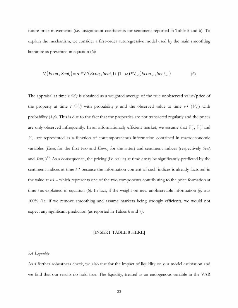
The appraisal at time t (Vt) is obtained as a weighted average of the true unobserved value/price of

the property at time t (Vt’) with probability p and the observed value at time t-1 (Vt-1) with

probability (1-p). This is due to the fact that the properties are not transacted regularly and the prices

are only observed infrequently. In an informationally efficient market, we assume that Vt , Vt’ and

Vt-1 are represented as a function of contemporaneous information contained in macroeconomic

variables (Econt for the first two and Econt-1 for the latter) and sentiment indices (respectively Sentt

and Sentt-1)13. As a consequence, the pricing (i.e. value) at time t may be significantly predicted by the

sentiment indices at time t-1 because the information content of such indices is already factored in

the value at t-1 – which represents one of the two components contributing to the price formation at

time t as explained in equation (6). In fact, if the weight on new unobservable information (p) was

100% (i.e. if we remove smoothing and assume markets being strongly efficient), we would not

expect any significant prediction (as reported in Tables 6 and 7).

[INSERT TABLE 8 HERE]

5.4 Liquidity

As a further robustness check, we also test for the impact of liquidity on our model estimation and

we find that our results do hold true. The liquidity, treated as an endogenous variable in the VAR

24

system, is significant in almost all models and boosts the goodness of fit, but the real estate

sentiment still remains significant for the residential market and insignificant for the non-residential

market. As a proxy for liquidity in the non-residential sector, we use a metric computed as the

difference between the demand and supply indices in percentage of the Transaction-Based Price

Index as the average of the two indices (Fisher et al., 2007). For the residential market, we use a

proxy for the funding liquidity measured by tightness levels in the banking system as provided by the

Federal Reserve Board through the Senior Loan Officer Opinion Survey on Bank Lending

Practices.14

5.5 Impulse Responses

Figures 1 and 2 present the impulse responses for the residential and non-residential sectors

respectively. In general, the directions of changes conform to our theoretical expectations.

Specifically for the residential model in Figure 1, a one standard deviation shock to our variable of

interest (‘pure’ component of the HMI) has a moderate positive short-run impact and overall

positive net impact. For the non-residential model (Figure 2), one standard deviation shock to the

‘pure’ component of ABI does not have any noticeable impact on changes in the TBI price index.

[INSERT FIGURES 1 AND 2 HERE]

5.6 Principal Component Analysis

It is quite likely that various sentiment measures will have some degree of commonality. The

presence of such common factors may prevent us from isolating the true effects. To explore this

issue further, we conduct a Principal Component Analysis (PCA) to extract common components

embedded in the sentiment measures (after performing the orthogonalization step). We have

25

conducted the PCA analysis for both the residential and non-residential sectors. By taking into

account five factors (as many as the sentiment indices used in our analysis for both the residential

and non-residential sector), we find that the previous results reported in Tables 4-7 hold true. Two

main factors for the residential sector are found to convey information and to contain predictive

power. We may interpret these two factors as measures reflecting general and real-estate specific

market sentiment. Finally, consistent with our results in Tables 5 and 6, no principal component is

significant in the non-residential market.

5.7 Out-of-sample Evaluation

To establish the importance of sentiment indicators in predicting real estate price changes, we have

also performed an out-of-sample test. To check the robustness of our out-of-sample evaluation, we

consider 1, 2 and 3-year evaluation windows and present selected forecast evaluation parameters in

Table 8. For the residential market (Panel A), there are improvements which are most prominent for

the 2- and 3-year windows. Both bias and variance proportion measures are generally small and the

covariance proportion measures reveal that the random component comprises more than the half of

the error (normally around 90-95%). Moreover, although in the out-of-sample evaluation exercise

we have perhaps chosen the worst time-period (in terms of economic uncertainties) the

improvement is still quite significant. Therefore, the out-of-sample predictions clearly show evidence

of a significant ‘gain’ in our forecasting ability when we incorporate indices based on the attitude

data and forward-looking surveys in the residential market (see also graph plotting actual values in

blue line against the forecast obtained with the hard economic data only in red line and the hard

economic data combined with the sentiment indices in green line).

26

For the non-residential market (Panel B), the results are less prominent, with a slightly higher bias

and variance proportion measures than those for the residential market. The gains obtained with the

inclusion of the sentiment indices are mainly achieved in the short-term (1-year forecast), even if the

Theil inequality coefficient reveals improvements in the 2- and 3-year forecasts too. Clearly, the out

of sample predictions do confirm that the non-residential sector is more informationally efficient

than the housing sector.

[INSERT TABLE 9 HERE]

6. Conclusion

In this study, we analyze the information content of several sentiment indices and their relative

importance in modeling real estate price changes. Due to several idiosyncrasies in the real estate

market such as infrequent transactions, lumpy investment and information asymmetry, this exercise

provides a good testing ground for analyzing the role of sentiment. Moreover, the real estate markets

(and particularly the residential sector) generally lead economic cycles. We employ a Vector Auto-

Regression (VAR) framework and use quarterly US data over 1988-2010 to test the predictability of

several sentiment measures. After testing for the stationarity, contemporaneous and inter-temporal

relationships, we estimate a VAR system. To extract the ‘pure’ sentiment effect, we orthogonalize

the sentiment measures against a set of macroeconomic variables. Overall, our analysis suggests that

the ‘pure’ sentiment in the residential sector may convey valuable information which should be

embedded in the modeling exercise to predict changes in the real estate returns. Our results suggest

that the sentiment indicators are important in explaining residential real estate price changes as there

are statistically significant information gains from using such survey-based indices. However, we do

27

not find any significant effects for the non-residential sector. Finally, our results are robust across

several model specifications, including the returns of a valuation-based index and common factors

of several sentiment measures estimated using a Principal Component Analysis.

Overall, our findings indicate that price changes in the residential sector respond significantly to

changes in sentiment, while the non-residential sector does not show any significant effects. This

may reflect a greater responsiveness of the residential market to shocks in ‘pure’ sentiment, possibly

being transmitted through the changes in the underlying demand shifters. Due to a typically inelastic

short-run supply curve in the residential market, any shift in the demand schedule is almost fully

reflected in the price change, with the short-run positive impact lasting for about two and a half

quarters. The consequent dampening of the effect may be attributed to a supply-side adjustment

mitigating the price effect. It can be argued that the role of uncertainty in transactions due to the

presence of significant information asymmetry (and therefore formation of future price expectation

by households) may be more prominent in the residential market than in the non-residential sector.

In fact, the extent of information asymmetry may be less prominent in generally more ‘informed’

non-residential markets, where economic agents – e.g. institutional investors – may have access to a

more comprehensive information set and their information processing may also be more formalized

than the agents in the residential sector. Another plausible explanation may be due to the nature of

contracting in the non-residential sector. Long-term contracts and complex price-setting exercises

may also prevent sentiment from influencing the pricing in the non-residential sector in the short

run. Future research may focus on the interaction of demand- and supply-side factors, investor type

and asymmetry in their behavior across various stages of the economic cycle. The evidences

provided in this paper suggest that there may be significant heterogeneity in information efficiency

28

across different sectors of the real estate market, which may stem from the variations in investment

patterns and channels in these sectors.

29

References

Akerlof, G. A. and R. J. Shiller, Animal Spirits. Princeton: Princeton University Press, 2009. Acemoglu, D. and A. Scott, Consumer confidence and rational expectations: are agents’ beliefs consistent with the theory? Economic Journal, 1994, 104, 1–19. Baker, M. and J. Wurgler, Investor sentiment and the cross-section of stock returns, Journal of Finance, 2006, 61, 1645–1680. Baker, M. and J. Wurgler, Investor sentiment in the stock market, Journal of Economic Perspectives, 2007, 21, 129-151. Baker, K. and D. Saltes, Architecture Billings as a Leading Indicator of Construction, Business Economics, 2005, October. Bram, J. and S. Ludvigson, Does Consumer Confidence Forecast Household Expenditure? A Sentiment Index Horse Race, FRBNY Economic Policy Review, 1998. Carroll, C. D., J. C. Fuhrer and D. W. Wilcox, Does consumer sentiment forecast household spending? If so, why? American Economic Review, 1994, 84, 1397–1408. Case, K. E. and R. J. Shiller, The Efficiency of the Market for Single-Family Homes, American Economic Review, 1989, 79, 125-137. Case, K. E. and R. J. Shiller, Is There a Bubble in the Housing Market? Brookings Papers on Economic Activity, 2003, 2, 300-361. Case, K. E., R. J. Shiller and A. Thompson, What Have They Been Thinking? Home Buyer Behavior in Hot and Cold Markets, NBER Working Paper Series No. 18400, 2012. Chang, C., P. H. Franses and M. McAleer, How accurate are government forecasts of economic fundamentals? The case of Taiwan, International Journal of Forecasting, 2011, 27(4), 1066-1075. Changha J., G. Soydemir and A. Tidwell, The U.S. Housing Market and the Pricing of Risk: Fundamental Analysis and Market Sentiment, Journal of Real Estate Research, 2014, 36(2). Chua, C. L. and S. Tsiaplias, Can Consumer Sentiment and its Components Forecast Australian GDP and Consumption? Journal of Forecasting, 2009, 28, 698–711. Clayton, J., D. Ling and A. Naranjo, Non-residential Real Estate Valuation: Fundamentals Versus Investor Sentiment, Journal of Real Estate Finance and Economics, 2009, 38(1), 5-37. Croce, R. M. and D. R. Haurin, Predicting turning points in the housing market, Journal of Housing Economics, 2009, 18, 281–293. Dua, P., Analysis of Consumers’ Perceptions of Buying Conditions for Houses, Journal of Real Estate Finance and Economics, 2008, 37, 335–350.

30

Easaw, J. Z. and S. M. Heravi, Evaluating consumer sentiments as predictors of UK household consumption behaviour: Are they accurate and useful? International Journal of Forecasting, 2004, 20(4), 671-681. Emrath, P., Housing Market Index, Housing Economics, National Association of Home Builders, Washington, DC. 1995, June. Fan, C. S. and P. Wong, Does consumer sentiment forecast household spending? the Hong Kong case, Economics Letters, 1998, 58(1), 77–84. Fuhrer, J. C. What Role Does Consumer Sentiment Play in the U.S. Economy? Federal Reserve Bank of Boston New England Economic Review, 1993, 32-44. Fisher, J., D. Geltner and H. Pollakowski, A Quarterly Transactions-based Index of Institutional Real Estate Investment Performance and Movements in Supply and Demand, Journal of Real Estate Finance and Economics, 2007, 34(1), 5-33. Goodman, J. L., Using attitude data to forecast housing activity, Journal of Real Estate Research, 1994, 9(4), 445–453. Hall, R. E. Stochastic implications of the life cycle-permanent income hypothesis: theory and evidence, Journal of Political Economy, 1978, 86 971-87. Hohenstatt, R. and M. Kaesbauer, ‘GECO’s Weather Forecast’ for the U.K. Housing Market: To What Extent Can We Rely on Google ECOnometrics? Journal of Real Estate Research, 2014, 36(2). Howrey, E. P. The Predictive Power of the Index of Consumer Sentiment, Brookings Papers on Economic Activity, 2001, 175-207. Joseph, K., J. Wintoki and Z. Zhang, Forecasting Abnormal Stock Returns and Trading Volume Using Investor Sentiment: Evidence from Online Search, International Journal of Forecasting, 2011, 27(4), 1116-1127. Jurgilas, M. and K. J. Lansing, Housing Bubbles and Expected Returns to Homeownership: Lessons and Policy Implications. Working paper, http//ssrn.com/abstract=2209719, 2013. Katona G., Psychological Economics, New York: Elsevier, 1975. Kumar, V. R. P. Leone and J. N. Gaskins, Aggregate and disaggregate sector forecasting using consumer confidence measures, International Journal of Forecasting, 1995, 11(3), 361-377. Lee, M., B. Elango and S. P. Schnaars, The accuracy of the Conference Board's buying plans index: A comparison of judgmental vs. extrapolation forecasting methods, International Journal of Forecasting, 1997, 13(1), 127-135. Linden, F., The Consumer as Forecaster, The Public Opinion Quarterly, 1982, 46(3), 353-360.

31

Ling, D., G. Marcato and P. McAllister, Dynamics of Asset Prices and Transaction Activity in Illiquid Markets: the Case of Private Non-residential Real Estate, Journal of Real Estate Finance and Economics, 2009, 39(3), 359-383. Ling, D., J. T. L. Ooi and T. T. Le, Explaining House Price Dynamics: Isolating the Role of Non-Fundamentals, Unpublished Working Paper, 2013. Ling, D., A. Naranjo and B. Scheick, Investor Sentiment, Limits to Arbitrage, and Private Market Returns, Real Estate Economics, 2013, 41(2), 1-47. Lizieri, C., G. Marcato, P. Ogden and A. Baum, Pricing Inefficiencies in Private Real Estate Markets Using Total Return Swaps, Journal of Real Estate Finance and Economics, 2012, 45(3), 774-803 Malgarini, M. and P. Margani, Psychology, consumer sentiment and household expenditures, Applied Economics, 2009, 39(13), 1719-1729. Matsusaka, J. G. and A. M. Sbordone, Consumer Confidence and Economic Fluctuations, Economic Inquiry, 1995, 33(2), 296-318. Milani, F., Expectation Shocks and Learning as Drivers of the Business Cycle, The Economic Journal, 2011, 121, 379–401. Mishkin, F. S. Consumer Sentiment and Spending on Durable Goods, Brookings Papers On Economic Activity, 1978, 1, 217-32. Nanda, A., Examining the NAHB/Wells Fargo Housing Market Index (HMI), Housing Economics, National Association of Home Builders, Washington, DC. March, 2007. Parigi, G. and G. Schlitzer, Predicting consumption of Italian households by means of survey indicators, International Journal of Forecasting, 1997, 13(2), 197-209. Piger, J. M. Consumer Confidence Surveys: Do They Boost Forecasters' Confidence? Regional Economist, Federal Reserve Bank of St. Louis, 2003, April. Quan, D. C. and J. M. Quigley, Inferring an investment return series for real estate from observations on sales, Journal of the American Real Estate and Urban Economics Association, 1989, 17, 218-30. Schmeling, M., Institutional and individual sentiment: Smart money and noise trader risk? International Journal of Forecasting, 2007, 23(1), 127-145. Shiller, R. J., Irrational Exuberance, Princeton, NJ: Princeton University Press, 2000. Souleles N., Expectations, heterogenous forecast errors and consumption: micro evidence from the Michigan consumer sentiment surveys, Journal of Money, Credit and Banking, 2004, 36, 39–72.

32

Stambaugh, R. F., J. Yu and Y. Yuan, The short of it: Investor sentiment and anomalies, Journal of Financial Economics, 2012, 104, 288–302. Tsolacos, S., C. Brooks and O. Nneji, On the Predictive Content of Leading Indicators: The Case of U.S. Real Estate Markets, Journal of Real Estate Research, Forthcoming. Utaka, A., Confidence and the real economy: the Japanese case, Applied Economics, 2003, 35, 337–342. Vuchelen, J., Consumer sentiment and macroeconomic forecasts, Journal of Economic Psychology, 2004, 25, 493–506. Wang, Y., A. Keswani and S. J. Taylor, The relationships between sentiment, returns and volatility, International Journal of Forecasting, 2006, 22(1), 109-123. Weber, W. and M. Devaney, Can consumer sentiment surveys forecast housing starts? Appraisal Journal, 1996, 4, 343–350.

33

Acknowledgement

The authors would like to acknowledge the financial support from the Royal Institution of

Chartered Surveyors (RICS) Education Trust, Real Estate Research Corporation (RERC) and

Henley Business School, University of Reading, School of Real Estate and Planning, UK. The

authors would also like to thank the two anonymous referees, Paul Emrath as well as participants at

the 2011 AREUEA Mid-Year Meeting for comments. Tumellano Sebehela provided excellent

research assistance. All remaining errors are ours.

Gianluca Marcato, Henley Business School, University of Reading, Reading, RG6 6UD, UK or g.marcato@reading.ac.uk. Anupam Nanda, Henley Business School, University of Reading, Reading, RG6 6UD, UK or : a.nanda@reading.ac.uk.

34

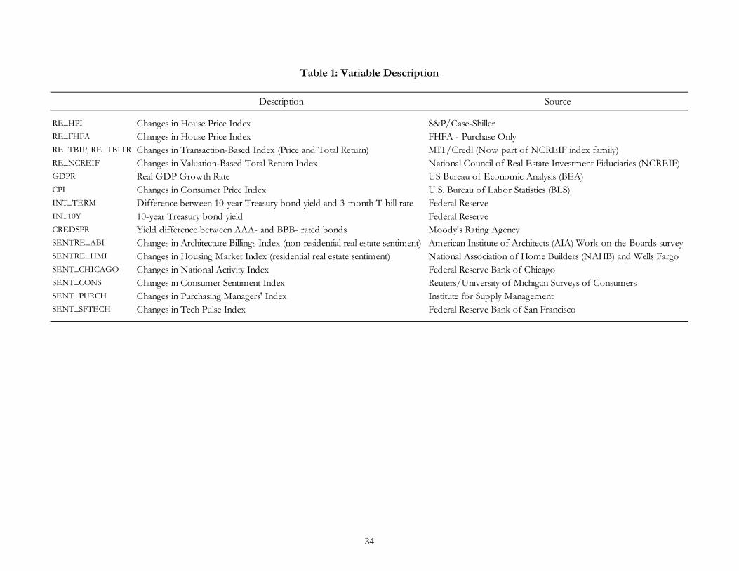
Table 1: Variable Description

Description Source

RE_HPI Changes in House Price Index S&P/Case-ShillerRE_FHFA Changes in House Price Index FHFA - Purchase OnlyRE_TBIP, RE_TBITR Changes in Transaction-Based Index (Price and Total Return) MIT/Credl (Now part of NCREIF index family)RE_NCREIF Changes in Valuation-Based Total Return Index National Council of Real Estate Investment Fiduciaries (NCREIF)GDPR Real GDP Growth Rate US Bureau of Economic Analysis (BEA)CPI Changes in Consumer Price Index U.S. Bureau of Labor Statistics (BLS)INT_TERM Difference between 10-year Treasury bond yield and 3-month T-bill rate Federal ReserveINT10Y 10-year Treasury bond yield Federal ReserveCREDSPR Yield difference between AAA- and BBB- rated bonds Moody's Rating AgencySENTRE_ABI Changes in Architecture Billings Index (non-residential real estate sentiment) American Institute of Architects (AIA) Work-on-the-Boards surveySENTRE_HMI Changes in Housing Market Index (residential real estate sentiment) National Association of Home Builders (NAHB) and Wells FargoSENT_CHICAGO Changes in National Activity Index Federal Reserve Bank of ChicagoSENT_CONS Changes in Consumer Sentiment Index Reuters/University of Michigan Surveys of Consumers SENT_PURCH Changes in Purchasing Managers' Index Institute for Supply ManagementSENT_SFTECH Changes in Tech Pulse Index Federal Reserve Bank of San Francisco

35

Table 2: Descriptive Statistics

Variables: RE_HPI = Changes in S&P/Case-Shiller Home Price Index; RE_FHFA = Changes in FHFA Purchase-only House Price Index; RE_TBIP = Changes in Transaction-Based Price Index; RE_TBITR = Changes in Transaction-Based Total Return Index; GDPR = Real GDP Growth Rate; CPI = Changes in Consumer Price Index; INT_TERM = Difference between 10-year Treasury bond yield and 3-month T-bill rate; INT10Y = 10-year Treasury bond yield; CREDSPR = Yield difference between AAA- and BBB- rated bonds; SENTRE_ABI = Changes in Architecture Billings Index (non-residential real estate sentiment); SENTRE_HMI = Changes in Housing Market Index (residential real estate sentiment); SENT_CHICAGO = Changes in National Activity Index; SENT_CONS = Changes in Consumer Sentiment Index; SENT_PURCH = Changes in Purchasing Managers' Index; SENT_SFTECH = Changes in Tech Pulse Index. The JB-stat indicates the value of the Jarque-Bera test and its p-value is in the next column. The ADF test reports the p-value of the statistic for the first lag with significant value (as suggested in the ‘Lag’ column). The maximum lag with the ADF test still being significant is reported in the ‘Max Lag’ column.

Mean Median Max Min Std. Dev. Skewness Kurtosis JB-stat Prob Sum Sum Sq. Dev. Obs Prob. Lag Max Lag

RE_HPI 0.9% 1.8% 4.4% -5.9% 2.52% -1.27 3.75 17.53 0.000 0.513 0.037 60 0.05 0 11RE_FHFA 0.8% 1.4% 2.6% -2.9% 1.44% -1.02 3.14 10.45 0.005 0.498 0.012 60 0.00 1 12RE_TBIP 1.0% 1.2% 16.4% -19.8% 5.2% -0.78 7.13 48.82 0.000 0.620 0.157 60 0.00 1 12RE_TBITR 2.4% 2.6% 17.4% -18.3% 5.13% -0.86 7.09 49.36 0.000 1.427 0.155 60 0.00 1 12RE_NCREIF 2.2% 2.8% 5.4% -8.3% 2.6% -2.37 9.09 149.07 0.000 1.349 0.041 60 0.00 4 12GDPR 0.6% 0.7% 1.9% -2.2% 0.71% -1.27 6.17 41.17 0.000 0.365 0.003 60 0.00 0 12CPI 0.6% 0.7% 1.5% -2.3% 0.56% -2.53 13.74 352.30 0.000 0.359 0.002 60 0.00 0 12INT_TERM 1.6% 1.5% 3.6% -0.6% 1.3% 0.06 1.69 4.31 0.116 0.949 0.009 60 0.02 1 12INT10Y 4.8% 4.7% 6.8% 2.7% 1.06% 0.15 2.25 1.65 0.437 2.860 0.007 60 0.16 0 12CREDSPR 1.02 0.91 3.37 0.57 0.49 3.04 13.98 393.80 0.000 61.110 14.303 60 0.00 1 12SENTRE_ABI 0.0% 1.8% 22.5% -28.7% 10.6% -0.32 3.16 1.07 0.586 0.025 0.660 60 0.00 0 10SENTRE_HMI -2.0% 0.0% 51.1% -63.6% 15.4% -0.65 7.90 64.14 0.000 -1.198 1.408 60 0.00 1 12SENT_CHICAGO 0.2% -6.3% 170.5% -211.5% 69.2% -0.18 3.42 0.75 0.687 0.111 28.246 60 0.00 0 12SENT_CONS -0.3% -0.2% 22.0% -22.2% 8.2% 0.10 4.47 5.48 0.065 -0.200 0.396 60 0.00 0 12SENT_PURCH 0.4% -0.1% 20.0% -27.4% 7.7% -0.21 5.15 11.96 0.003 0.236 0.349 60 0.00 0 12SENT_SFTECH 1.8% 2.3% 12.1% -13.5% 5.2% -0.73 3.62 6.31 0.043 1.080 0.161 60 0.00 0 12

Statistics Normality ADF Test

36

Table 3: Granger Causality Tests

Panel A: Residential Real Estate

Panel B: Non-residential Real Estate

Variables: RE_TBIP = Changes in Transaction-Based Price Index; RE_HPI = Changes in S&P/Case-Shiller Home Price Index; GDP = Real GDP Growth Rate; CPI = Changes in Consumer Price Index; INT_TERM = Difference between 10-year Treasury bond yield and 3-month T-bill rate; INT10Y = 10-year Treasury bond yield; CREDSPR = Yield difference between AAA- and BBB- rated bonds; SENTRE_ABI = Changes in Architecture Billings Index (non-residential real estate sentiment); SENTRE_HMI = Changes in Housing Market Index (residential real estate sentiment); SENT_CHICAGO = Changes in National Activity Index; SENT_CONS = Changes in Consumer Sentiment Index; SENT_PURCH = Changes in Purchasing Managers' Index; SENT_SFTECH = Changes in Tech Pulse Index. Grange Causality tests are run between each economic data/ sentiment index and real estate price changes for different lags (1 to 12). Start and End report respectively the initial and last lag for which Granger-causality is found (i.e. no causality is found before the starting or after the ending quarter). * The P-values of the coefficients of causation (‘causing’ for economic data / sentiment indices causing real estate price changes, ‘caused’ for economic data caused by real estate price changes) are reported only for the equations when causation starts. For example in Panel A, 0.0127 is the p-value of economic data/sentiment indices Granger causing real estate price changes with one quarter lag (Q1 for ‘Start’), while 0.7918 is the p-value of real estate price changes causing economic data/sentiment indices with 1 quarter lag. Since only the former shows statistical significance with confidence set at 95% level, we conclude that GDP Granger-causes real estate price changes. Initial reversal reports the initial lags when a causation opposite to the one shown by the p-values is found. For Example in Panel A, since SENT_CHICAGO is found to cause real estate price changes from Q3 to Q12 (see p-values of Q3 in the fourth and fifth column), an initial reversal Q1-Q2 indicates that real estate price changes Granger-cause general sentiment (Chicago) in these two quarters. No value in initial reversal indicates that opposite causation is not found at any lag.

Initial Start End Causing Caused Reversal

GDP Q7 Q7 0.008 0.112 -CPI Q3 Q5 0.000 0.330 -INT_TERM - - 0.217 0.002 Q1INT10Y Q11 Q12 0.037 0.208 -CREDSPR - - 0.207 0.008 Q1SENTRE_HMI Q1 Q5 0.028 0.532 -SENT_CHICAGO Q1 Q6 0.002 0.996 Q11SENT_CONS - - 0.233 0.821 -SENT_PURCH Q1 Q6 0.021 0.635 -SENT_SFTECH - - 0.505 0.643 Q5-Q7

Granger Causality P-value*

* The P-value refers to the starting quarter when the variable granger causes real estate total returns

Initial Start End Causing Caused Reversal

GDP Q1 Q5 0.013 0.792 -CPI Q6 Q6 0.049 0.411 -INT_TERM Q3 Q6 0.014 0.193 Q1INT10Y - - 0.444 0.930 -CREDSPR Q1 Q12 0.000 0.495SENTRE_ABI Q3 Q10 0.015 0.912 -SENT_CHICAGO Q3 Q12 0.000 0.130 Q1SENT_CONS - - 0.728 0.001 Q1SENT_PURCH Q7 Q8 0.040 0.286 Q1SENT_SFTECH Q1 Q1 0.042 0.758 -

Granger Causality P-value*

* The P-value refers to the starting quarter when the variable granger causes real estate total returns

37

Table 4: VAR Estimation with Real Price Changes: Residential Real Estate-I (S&P/Case-Shiller Home Price Index)

Dependent Variable: HPI = Changes in S&P/Case-Shiller Home Price Index. Independent Variables: Real Estate Sentiment = Changes in the orthogonalized Housing Market Index (residential sentiment index); General Sentiment = Changes in the orthogonalized general sentiment index (Chicago = Changes in National Activity Index; Consumer = Changes in Consumer Sentiment Index; Purchase = Changes in Purchasing Managers' Index; SFTech = Changes in Tech Pulse Index). Macro-economic variables included in the model: GDP = Real GDP Growth Rate; Inflation rate = Changes in Consumer Price Index; Real interest rate = 10-year Treasury bond yield net of inflation; Term Spread = Difference between 10-year Treasury bond yield and 3-month T-bill rate; Credit Spread = Yield difference between AAA- and BBB- rated bonds. Notes: Only the outcome from the price changes equation in the VAR system is reported in the table under each column. Sample period is 1988Q3-2010Q4. The p-values from the joint significance across the lags are reported in the Granger-Causality section of the table. t-stats are reported underneath the coefficient estimates. P-values in bold show significance up to 5% level. P-values in bold and italics show significance up to 10% level.

Return Equation Model 1 Model 2 Model 3 Model 4 Model 5 Model 6Chicago Consumer Purchase SFTech

AR1 0.691*** 0.617*** 0.627*** 0.622*** 0.633*** 0.61***6.996 5.933 5.932 5.889 5.864 5.674

AR2 0.150 0.243** 0.243** 0.233** 0.231** 0.221**1.542 2.371 2.320 2.245 2.163 2.097

Real Estate Sentiment (-1) 0.025*** 0.022** 0.026** 0.021** 0.026***2.669 2.350 2.429 2.128 2.729

Real Estate Sentiment (-2) -0.010 -0.010 -0.010 -0.010 -0.010-1.557 -1.614 -0.821 -1.536 -1.477

General Sentiment (-1) 0.005** -0.010 0.030 0.0002.340 -0.371 1.457 0.085

General Sentiment (-2) 0.000 -0.020 -0.010 -0.030-0.156 -1.016 -0.686 -0.949

Constant 0.000 0.004* 0.005** 0.000 0.005* 0.0001.040 1.745 2.024 1.578 1.795 1.520

Macro-economic variables YES YES YES YES YES YES

Adj. R-squared 0.71 0.74 0.75 0.73 0.74 0.73 F-statistic 33.41 29.76 26.45 24.16 24.90 24.13 Log likelihood 291.78 297.33 301.18 297.92 299.00 297.88 Akaike AIC -6.10 -6.18 -6.22 -6.15 -6.17 -6.15 Schwarz SC -5.89 -5.91 -5.89 -5.82 -5.85 -5.82

Granger-Causality (p-values)Real Estate Sentiment 0.005 0.010 0.034 0.024 0.005General Sentiment 0.030 0.597 0.227 0.619

38

Table 5: VAR Estimation with Real Price Changes: Residential Real Estate-II (FHFA House Price Index)

Dependent Variable: HPI = Changes in FHFA House Price Index. Independent Variables: Real Estate Sentiment = Changes in the orthogonalized Housing Market Index (residential sentiment index); General Sentiment = Changes in the orthogonalized general sentiment index (Chicago = Changes in National Activity Index; Consumer = Changes in Consumer Sentiment Index; Purchase = Changes in Purchasing Managers' Index; SFTech = Changes in Tech Pulse Index). Macro-economic variables included in the model: GDP = Real GDP Growth Rate; Inflation rate = Changes in Consumer Price Index; Real interest rate = 10-year Treasury bond yield net of inflation; Term Spread = Difference between 10-year Treasury bond yield and 3-month T-bill rate; Credit Spread = Yield difference between AAA- and BBB- rated bonds. Notes: Only the outcome from the price changes equation in the VAR system is reported in the table under each column. Sample period is 1988Q3-2010Q4. The p-values from the joint significance across the lags are reported in the Granger-Causality section of the table. T-stats are reported underneath the coefficient estimates. P-values in bold show significance up to 5% level. P-values in bold and italics show significance up to 10% level.

Return Equation Model 1 Model 2 Model 3 Model 4 Model 5 Model 6Chicago Consumer Purchase SFTech

AR1 0.468*** 0.451*** 0.451*** 0.498*** 0.443*** 0.458***5.891 5.834 5.709 6.564 5.721 5.836

AR2 0.509*** 0.514*** 0.514*** 0.484*** 0.53*** 0.535***5.884 6.122 5.973 6.006 6.216 5.789

Real Estate Sentiment (-1) 0.000 0.000 0.011** 0.010 0.0000.840 0.880 2.065 1.194 0.906

Real Estate Sentiment (-2) 0.015*** 0.015*** 0.01* 0.014** 0.015***2.790 2.724 1.798 2.521 2.843

General Sentiment (-1) 0.000 -0.017** -0.010 0.020-0.261 -2.142 -1.301 0.890

General Sentiment (-2) 0.000 0.010 0.010 0.000-0.280 1.457 0.564 -0.240

Constant 0.005*** 0.005*** 0.005*** 0.005*** 0.005*** 0.005***4.248 4.080 3.885 4.717 4.003 4.046

Macro-economic variables YES YES YES YES YES YES

Adj. R-squared 0.85 0.87 0.86 0.88 0.87 0.86 F-statistic 64.66 55.94 44.48 52.74 46.10 45.02 Log likelihood 304.84 309.42 309.48 315.33 310.70 309.89 Akaike AIC -7.71 -7.78 -7.73 -7.88 -7.76 -7.74 Schwarz SC -7.47 -7.47 -7.36 -7.51 -7.39 -7.37

Granger-Causality (p-values)Real Estate Sentiment 0.015 0.017 0.023 0.018 0.012General Sentiment 0.949 0.005 0.333 0.672

39

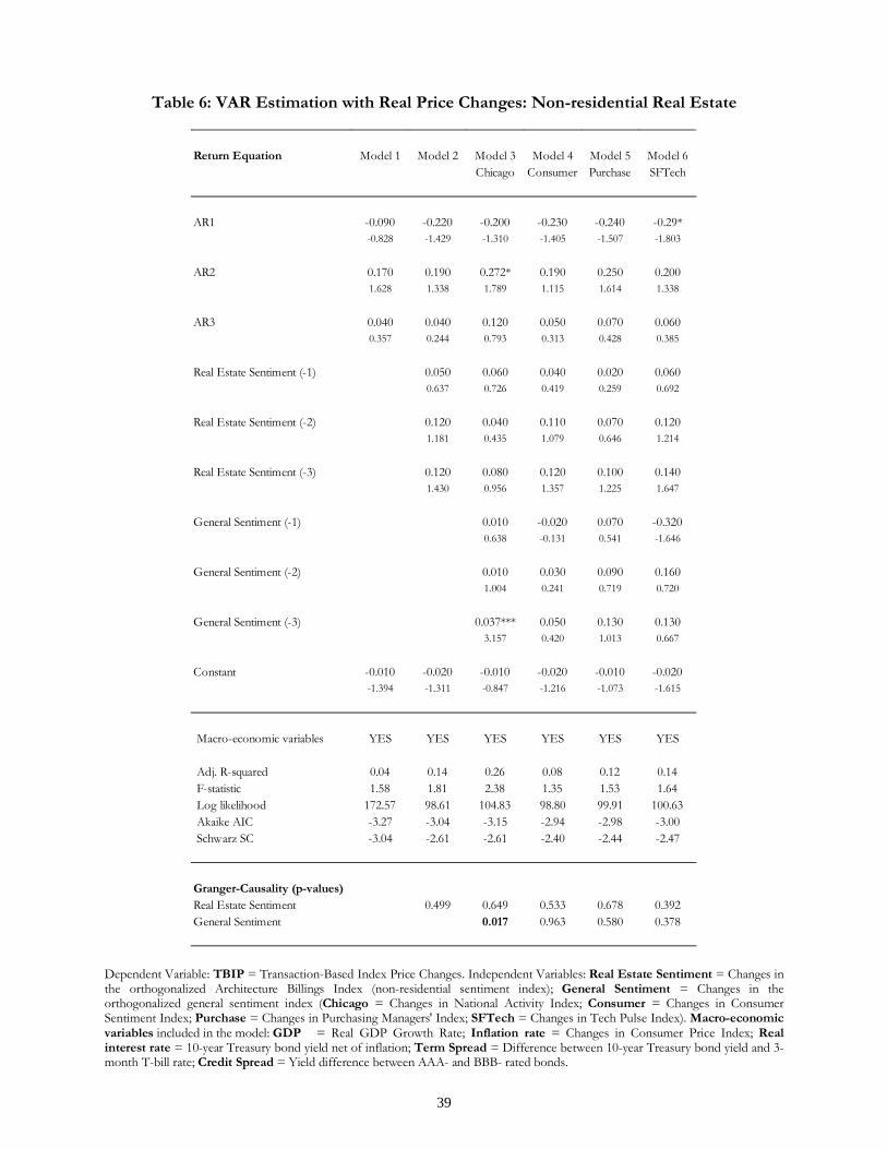
Table 6: VAR Estimation with Real Price Changes: Non-residential Real Estate

Dependent Variable: TBIP = Transaction-Based Index Price Changes. Independent Variables: Real Estate Sentiment = Changes in the orthogonalized Architecture Billings Index (non-residential sentiment index); General Sentiment = Changes in the orthogonalized general sentiment index (Chicago = Changes in National Activity Index; Consumer = Changes in Consumer Sentiment Index; Purchase = Changes in Purchasing Managers' Index; SFTech = Changes in Tech Pulse Index). Macro-economic variables included in the model: GDP = Real GDP Growth Rate; Inflation rate = Changes in Consumer Price Index; Real interest rate = 10-year Treasury bond yield net of inflation; Term Spread = Difference between 10-year Treasury bond yield and 3-month T-bill rate; Credit Spread = Yield difference between AAA- and BBB- rated bonds.

Return Equation Model 1 Model 2 Model 3 Model 4 Model 5 Model 6Chicago Consumer Purchase SFTech

AR1 -0.090 -0.220 -0.200 -0.230 -0.240 -0.29*-0.828 -1.429 -1.310 -1.405 -1.507 -1.803

AR2 0.170 0.190 0.272* 0.190 0.250 0.2001.628 1.338 1.789 1.115 1.614 1.338

AR3 0.040 0.040 0.120 0.050 0.070 0.0600.357 0.244 0.793 0.313 0.428 0.385

Real Estate Sentiment (-1) 0.050 0.060 0.040 0.020 0.0600.637 0.726 0.419 0.259 0.692

Real Estate Sentiment (-2) 0.120 0.040 0.110 0.070 0.1201.181 0.435 1.079 0.646 1.214

Real Estate Sentiment (-3) 0.120 0.080 0.120 0.100 0.1401.430 0.956 1.357 1.225 1.647

General Sentiment (-1) 0.010 -0.020 0.070 -0.3200.638 -0.131 0.541 -1.646

General Sentiment (-2) 0.010 0.030 0.090 0.1601.004 0.241 0.719 0.720

General Sentiment (-3) 0.037*** 0.050 0.130 0.1303.157 0.420 1.013 0.667

Constant -0.010 -0.020 -0.010 -0.020 -0.010 -0.020-1.394 -1.311 -0.847 -1.216 -1.073 -1.615

Macro-economic variables YES YES YES YES YES YES

Adj. R-squared 0.04 0.14 0.26 0.08 0.12 0.14 F-statistic 1.58 1.81 2.38 1.35 1.53 1.64 Log likelihood 172.57 98.61 104.83 98.80 99.91 100.63 Akaike AIC -3.27 -3.04 -3.15 -2.94 -2.98 -3.00 Schwarz SC -3.04 -2.61 -2.61 -2.40 -2.44 -2.47

Granger-Causality (p-values)Real Estate Sentiment 0.499 0.649 0.533 0.678 0.392General Sentiment 0.017 0.963 0.580 0.378

40

Notes: Only the outcome from the price changes equation in the VAR system is reported in the table under each column. Sample period is 1997Q1-2010Q4. The p-values from the joint significance across the lags are reported in the Granger-Causality section of the table. t-stats are reported underneath the coefficient estimates. P-values in bold show significance up to 5% level. P-values in bold and italics show significance up to 10% level.

41

Table 7: VAR Estimation with Real Total Returns: Non-residential Real Estate

Dependent Variable: TBITR = Transaction-Based Index Total Returns. Independent Variables: Real Estate Sentiment = Changes in the orthogonalized Architecture Billings Index (non-residential sentiment index); General Sentiment = Changes in the orthogonalized general sentiment index (Chicago = Changes in National Activity Index; Consumer = Changes in Consumer Sentiment Index; Purchase = Changes in Purchasing Managers' Index; SFTech = Changes in Tech Pulse Index). Macro-economic variables included in the model: GDP = Real GDP Growth Rate; Inflation rate = Changes in Consumer Price Index; Real interest rate = 10-year Treasury bond yield net of inflation; Term Spread = Difference between 10-year Treasury bond yield and 3-month T-bill rate; Credit Spread = Yield difference between AAA- and BBB- rated bonds. Notes: Only the outcome from price changes equation in the VAR system is reported in the table under each column. Sample period is 1997Q1-2010Q4. The p-values from the joint significance across the lags are reported in the Granger-Causality section of the table. t-stats are reported underneath the coefficient estimates. P-values in bold show significance up to 5% level. P-values in bold and italics show significance up to 10% level.

Return Equation Model 1 Model 2 Model 3 Model 4 Model 5 Model 6Chicago Consumer Purchase SFTech

AR1 -0.090 -0.200 -0.180 -0.210 -0.220 -0.274*-0.790 -1.319 -1.180 -1.282 -1.381 -1.687

AR2 0.170 0.200 0.287* 0.200 0.250 0.1901.538 1.330 1.849 1.135 1.592 1.299

AR3 0.040 0.050 0.130 0.070 0.080 0.0700.413 0.315 0.871 0.414 0.501 0.452

Real Estate Sentiment (-1) 0.040 0.050 0.030 0.020 0.0500.541 0.606 0.340 0.189 0.590

Real Estate Sentiment (-2) 0.100 0.030 0.100 0.060 0.1101.052 0.290 0.973 0.555 1.081

Real Estate Sentiment (-3) 0.110 0.060 0.110 0.090 0.1301.286 0.799 1.206 1.091 1.497

General Sentiment (-1) 0.010 -0.010 0.070 -0.3200.751 -0.068 0.535 -1.600

General Sentiment (-2) 0.010 0.050 0.090 0.1601.124 0.352 0.712 0.705

General Sentiment (-3) 0.037*** 0.050 0.120 0.1403.144 0.423 0.933 0.667

Constant 0.000 0.000 0.000 0.000 0.000 -0.010-0.128 -0.227 0.081 -0.193 -0.102 -0.530

Macro-economic variables YES YES YES YES YES YES

Adj. R-squared 0.04 0.12 0.24 0.06 0.09 0.11 F-statistic 1.54 1.67 2.24 1.25 1.40 1.52 Log likelihood 172.70 98.20 104.38 98.40 99.37 100.14 Akaike AIC -3.27 -3.02 -3.14 -2.93 -2.96 -2.99 Schwarz SC -3.04 -2.59 -2.60 -2.39 -2.42 -2.45

Granger-Causality (p-values)Real Estate Sentiment 0.594 0.737 0.624 0.753 0.484General Sentiment 0.017 0.961 0.623 0.400

42

Table 8: VAR Estimation with Valuation-Based Real Total Returns: Non-residential Real Estate

Dependent Variable: NCREIF = Valuation-based NCREIF Total Return Index. Independent Variables: Real Estate Sentiment = Changes in the orthogonalized Architecture Billings Index (non-residential sentiment index); General Sentiment = Changes in the orthogonalized general sentiment index (Chicago = Changes in National Activity Index; Consumer = Changes in Consumer Sentiment Index; Purchase = Changes in Purchasing Managers' Index; SFTech = Changes in Tech Pulse Index). Macro-economic variables included in the model: GDP = Real GDP Growth Rate; Inflation rate = Changes in Consumer Price Index; Real

Return Equation Model 1 Model 2 Model 3 Model 4 Model 5 Model 6Chicago Consumer Purchase SFTech

AR1 0.726*** 0.919*** 0.913*** 0.998*** 0.928*** 0.953***8.059 9.439 8.859 9.554 8.892 9.321

AR2 0.312*** 0.228** 0.224* 0.100 0.217* 0.225**3.347 2.165 1.963 0.830 1.950 2.091

AR3 -0.184** -0.281*** -0.272*** -0.265*** -0.3*** -0.298***-2.138 -3.169 -2.849 -3.010 -2.985 -3.205

Real Estate Sentiment (-1) 0.032** 0.033* 0.020 0.033* 0.029*2.007 1.939 1.076 1.925 1.761

Real Estate Sentiment (-2) 0.020 0.020 0.020 0.030 0.0201.281 1.165 1.278 1.293 1.219

Real Estate Sentiment (-3) 0.030 0.030 0.020 0.030 0.0201.559 1.483 1.367 1.519 1.183

General Sentiment (-1) 0.000 -0.06*** -0.020 0.050-0.134 -2.979 -0.608 1.135

General Sentiment (-2) 0.000 0.000 -0.010 -0.0700.009 0.197 -0.198 -1.569

General Sentiment (-3) 0.000 0.010 -0.010 0.0400.315 0.632 -0.177 0.910

Constant 0.000 0.000 0.000 0.000 0.000 0.0000.695 0.923 0.806 0.887 0.796 0.931

Macro-economic variables YES YES YES YES YES YES

Adj. R-squared 0.73 0.86 0.85 0.88 0.85 0.86 F-statistic 35.37 32.14 23.66 31.73 23.85 25.47 Log likelihood 308.66 189.96 190.05 197.59 190.25 191.92 Akaike AIC -5.93 -6.24 -6.14 -6.41 -6.15 -6.21 Schwarz SC -5.70 -5.81 -5.60 -5.87 -5.61 -5.67

Granger-Causality (p-values)Real Estate Sentiment 0.086 0.106 0.392 0.113 0.231General Sentiment 0.987 0.005 0.932 0.392

43

interest rate = 10-year Treasury bond yield net of inflation; Term Spread = Difference between 10-year Treasury bond yield and 3-month T-bill rate; Credit Spread = Yield difference between AAA- and BBB- rated bonds. Notes: Only the outcome from the price changes equation in the VAR system is reported in the table under each column. Sample period is 1988Q3-2010Q4. The p-values from the joint significance across the lags are reported in the Granger-Causality section of the table. t-stats are reported underneath the coefficient estimates. P-values in bold show significance up to 5% level. P-values in bold and italics show significance up to 10% level.

44

Table 9: Out-of-sample Predictions (Forecasts 2008-10)

Panel A: Residential Market

Notes: The sample period is 1997Q1 to 2010Q4. Model (1) – hard economic data only – and model (6) – hard economic data & both general and real estate sentiment indicators – in Table 4 are used for these predictions. ‘Forecasts 2008-10’ indicate that models are estimated using the sample 1997Q1 to 2007Q4 and the out-of-sample period refers to 2008Q1 to 2010Q4.

Notes: These forecasts are based on the non-residential models reported in Table 4. The blue line represents actual real estate price changes for the out-of-sample prediction, the red line represents out-of-sample forecasts obtained with a model only including economic variables and the green line represents out-of-sample forecasts obtained with a model including both economic variables and sentiment indicators. Source: Authors’ calculation.

Root Mean Squared Error 2.39% 2.13% 2.71% 2.19% 2.67% 2.21%Bias Proportion 0.96% 5.65% 12.90% 0.58% 1.15% 2.01%Variance Proportion 1.04% 7.18% 28.13% 7.17% 8.60% 2.81%Covariance Proportion 98.00% 87.17% 58.96% 92.25% 90.25% 95.18%

Theil Inequality Coefficient 2.3% 1.9% 2.7% 2.5% 3.2% 2.9%Mean Absolute Error 2.03% 1.49% 2.48% 1.66% 2.39% 1.68%Mean Absolute Percentage Error 0.60 0.51 4.12 2.00 2.99 1.53

Economic Economic& Sentiment

Economic Economic& Sentiment

Economic Economic& Sentiment

1 Year Forecast 2 Year Forecast 3 Year Forecast

60

65

70

75

80

85

90

95

100

105

Inde

x Val

ue

Time

Actual Forecast Economy Forecast Economy & Sentiment

45

Panel B: Non-Residential Market

Notes: The sample period is 1997Q1 to 2010Q4. Model (1) – hard economic data only – and model (3) – hard economic data & both general and real estate sentiment indicators – in Table 6 are used for these predictions. ‘Forecasts 2008-10’ indicate that models are estimated using the sample 1997Q1 to 2007Q4 and the out-of-sample period refers to 2008Q1 to 2010Q4.

Notes: These forecasts are based on the non-residential models reported in Table 6. The blue line represents actual real estate price changes for the out-of-sample prediction, the red line represents out-of-sample forecasts obtained with a model only including economic variables and the green line represents out-of-sample forecasts obtained with a model including both economic variables and sentiment indicators. Source: Authors’ calculation.

Root Mean Squared Error 4.06% 2.51% 8.97% 9.66% 8.26% 8.50%Bias Proportion 27.88% 0.39% 29.55% 27.48% 7.23% 18.19%Variance Proportion 68.49% 21.14% 23.25% 3.67% 49.01% 14.90%Covariance Proportion 0.42% 78.47% 47.20% 68.85% 43.76% 66.91%

Theil Inequality Coefficient 66.4% 3.8% 84.4% 24.5% 84.9% 19.5%Mean Absolute Error 3.21% 2.34% 5.60% 6.16% 5.93% 5.53%Mean Absolute Percentage Error 1.20 1.88 1.03 1.58 0.97 1.26

Economic Economic& Sentiment

Economic Economic& Sentiment

3 Year Forecast

Economic Economic& Sentiment

2 Year Forecast1 Year Forecast

0

20

40

60

80

100

120

140

Inde

x Val

ue

Time

Actual Forecast Economy Forecast Economy & Sentiment

46

Figure 1: Impulse Responses: Residential Real Estate

Variables: AR Process = Autoregressive Component of the S&P/Case-Shiller Home Price index; Real Estate Sentiment HMI = Changes in the orthogonalized Housing Market Index (residential sentiment index); General Sentiment = Changes in orthogonalized general sentiment index (Chicago = National Activity Index; Consumer = Consumer Sentiment Index; Purchase = Purchasing Managers' Index; SFTech = Tech Pulse Index). Notes: Graphs represent impulse responses of residential real estate price changes to innovations in sentiment indices. All impulse responses are derived from Table 4. Source: Authors’ calculation.

-.004

.000

.004

.008

.012

1 2 3 4 5 6 7 8 9 10

-.004

.000

.004

.008

.012

1 2 3 4 5 6 7 8 9 10

-.004

.000

.004

.008

.012

1 2 3 4 5 6 7 8 9 10

-.004

.000

.004

.008

.012

.016

1 2 3 4 5 6 7 8 9 10

-.004

.000

.004

.008

.012

.016

1 2 3 4 5 6 7 8 9 10

-.004

.000

.004

.008

.012

.016

1 2 3 4 5 6 7 8 9 10

AR process Real Estate Sentiment: HMI

General Sentiment: Chicago

General Sentiment: SFTechGeneral Sentiment: Purchase

General Sentiment: Consumer

Retu

rnRe

turn

Retu

rn

47

Figure 2: Impulse Responses: Non-residential Real Estate

Variables: AR Process = Autoregressive Component of the Real Transaction-Based Price Index; Real Estate Sentiment ABI = Changes in the orthogonalized Architecture Billings Index (non-residential sentiment index); General Sentiment = Changes in orthogonalized general sentiment index (Chicago = National Activity Index; Consumer = Consumer Sentiment Index; Purchase = Purchasing Managers' Index; SFTech = Tech Pulse Index). Notes: Graphs represent impulse responses of non-residential real estate price changes to innovations in sentiment indices. All impulse responses are derived from Table 6. Source: Authors’ calculation.

-.04

-.02

.00

.02

.04

.06

1 2 3 4 5 6 7 8 9 10

-.04

-.02

.00

.02

.04

.06

1 2 3 4 5 6 7 8 9 10

-.04

-.02

.00

.02

.04

.06

1 2 3 4 5 6 7 8 9 10

-.04

-.02

.00

.02

.04

.06

1 2 3 4 5 6 7 8 9 10

-.04

-.02

.00

.02

.04

.06

1 2 3 4 5 6 7 8 9 10

-.04

-.02

.00

.02

.04

.06

1 2 3 4 5 6 7 8 9 10

p _ _

AR process Real Estate Sentiment: ABI

General Sentiment: Chicago

General Sentiment: SFTechGeneral Sentiment: Purchase

General Sentiment: Consumer

Retu

rnRe

turn

Retu

rn

48

1 See Milani (2011) for a recent paper on relaxing rational expectation assumption. Also see paper on investors’ sentiment by Wang, Keswani and Taylor (2006); Schmeling (2007); Joseph, Wintoki and Zhang (2011); Stambaugh, Yu and Yuan (2012).

2 Lee, M., Elango, B. & Schnaars, S. P. (1997) find very little support for using Conference Board’s buying intention data for forecasting sales of durable goods. Also see, Fuhrer (1993), Howrey (2001) and Piger (2003).

3 Ling et al., 2009 find that in UK private real estate, asset turnover provides increased price revelation which may reduce investment risk and thus increases the property values.

4 see http://www.ncreif.org/tbi-returns.aspx

5 For details, see American Institute of Architects (AIA) Work-on-the-Boards survey - http://www.aia.org/practicing/economics/AIAS076265

6 For details, see The NAHB/Wells Fargo Housing Market Index (HMI): http://www.nahb.org/reference_list.aspx?sectionID=134

7 For details, see The Chicago Fed National Activity Index (CFNAI) - http://www.chicagofed.org/webpages/publications/cfnai/index.cfm

8 For details, see The Reuters/University of Michigan Surveys of Consumers: https://customers.reuters.com/community/university/default.aspx

9 For details, see The Purchasing Managers Index (PMI): http://www.ism.ws/ISMReport/content.cfm?ItemNumber=10752&navItemNumber=12961

10 For details, see The Tech Pulse Index: http://www.frbsf.org/csip/pulse.php

11 We also perform Phillips-Perron (PP) test for detecting unit roots and we do not find any significantly different outcome

12 This empirical discussion is drawn from Enders (2010), Chapter 5.

13 This is the reason why we inserted Econ and Sent within brackets next to the variables V in equation (6). For example Vt(Econt,Sentt) means that the variable Vt is a function of Econt and Sentt, i.e. the value of a property at time t is a function of the information set contained in macro-economic variables and sentiment measures released at time t.

14 Source: http://www.federalreserve.gov/boarddocs/snloansurvey/.