Information-driven experimental design in materials science R. Aggarwal, M. J. Demkowicz, Y. M. Marzouk Abstract Optimal experimental design (OED) aims to maximize the value of experiments and the data they produce. OED ensures efficient allocation of limited resources, especially when numerous repeated experiments cannot be performed. This chapter presents a fully Bayesian and decision theoretic approach to OED—accounting for uncertainties in models, model parameters, and experimental outcomes, and allowing optimality to be defined according to a range of possible experimental goals. We demonstrate this approach on two illustrative problems in materials research. The first example is a parameter inference problem. Its goal is to determine a sub- strate property from the behavior of a film deposited thereon. We design experiments to yield maximal information about the substrate property using only two measure- ments. The second example is a model selection problem. We design an experiment that optimally distinguishes between two models for helium trapping at interfaces. In both instances, we provide model-based justifications for why the selected experi- ments are optimal. Moreover, both examples illustrate the utility of reduced-order or surrogate models in optimal experimental design. 1 Introduction Experiments are essential prerequisites of all scientific research. They are the basis for developing and refining mathematical models of physical reality. Experimental data are used to infer model parameters, to improve the accuracy of model-based predictions, to discriminate among competing models, to assess model validity, and to improve design and decision-making under uncertainty. Yet experimental observations can be difficult, time-consuming, and expensive to acquire. Maximizing the value of exper- imental observations—i.e., designing experiments to be optimal by some appropriate measure—is therefore a critical task. Experimental design encompasses questions of where and when to measure, which variables to interrogate, and what experimental conditions to employ. Conventional experimental design methods, such as factorial and composite de- signs, are largely used as heuristics for exploring the relationship between input factors and response variables. By contrast, optimal experimental design uses a concrete hypothesis—expressed as a quantitative model—to guide the choice of experiments for a particular purpose, such as parameter inference, prediction, or model discrimi- nation. Optimal design has seen extensive development for linear models (where the measured quantities depend linearly on the model parameters) endowed with Gaussian 1
Transcript
Information-driven experimental design in materials science
R. Aggarwal, M. J. Demkowicz, Y. M. Marzouk
AbstractOptimal experimental design (OED) aims to maximize the value of experiments and
the data they produce. OED ensures e�cient allocation of limited resources, especiallywhen numerous repeated experiments cannot be performed. This chapter presents afully Bayesian and decision theoretic approach to OED—accounting for uncertaintiesin models, model parameters, and experimental outcomes, and allowing optimality tobe defined according to a range of possible experimental goals. We demonstrate thisapproach on two illustrative problems in materials research.
The first example is a parameter inference problem. Its goal is to determine a sub-strate property from the behavior of a film deposited thereon. We design experimentsto yield maximal information about the substrate property using only two measure-ments. The second example is a model selection problem. We design an experimentthat optimally distinguishes between two models for helium trapping at interfaces.In both instances, we provide model-based justifications for why the selected experi-ments are optimal. Moreover, both examples illustrate the utility of reduced-order orsurrogate models in optimal experimental design.
1 IntroductionExperiments are essential prerequisites of all scientific research. They are the basis fordeveloping and refining mathematical models of physical reality. Experimental data areused to infer model parameters, to improve the accuracy of model-based predictions,to discriminate among competing models, to assess model validity, and to improvedesign and decision-making under uncertainty. Yet experimental observations can bedi�cult, time-consuming, and expensive to acquire. Maximizing the value of exper-imental observations—i.e., designing experiments to be optimal by some appropriatemeasure—is therefore a critical task. Experimental design encompasses questions ofwhere and when to measure, which variables to interrogate, and what experimentalconditions to employ.
Conventional experimental design methods, such as factorial and composite de-signs, are largely used as heuristics for exploring the relationship between input factorsand response variables. By contrast, optimal experimental design uses a concretehypothesis—expressed as a quantitative model—to guide the choice of experimentsfor a particular purpose, such as parameter inference, prediction, or model discrimi-nation. Optimal design has seen extensive development for linear models (where themeasured quantities depend linearly on the model parameters) endowed with Gaussian
1
distributions [5]. Extensions to nonlinear models are often based on linearization andGaussian approximations [15, 36, 21], as analytical results are otherwise impracticalor impossible to obtain. With advances in computational power, however, optimalexperimental design for nonlinear systems can now be tackled directly using numericalsimulation [65, 84, 93, 64, 89, 48, 49, 96].
This chapter will present an overview of model-based optimal experimental design,connecting this approach to illustrative applications in materials science—a field repletewith potential applications for optimal experimentation. We will take a fully Bayesianand decision-theoretic approach. In this formulation, one first defines the utility of anexperiment and then, taking into account uncertainties in both the parameter valuesand the observations, chooses experiments by maximizing an expected utility. We willdefine these utilities according to information theoretic considerations, reflecting theparticular experimental goals at hand.
The evaluation and optimization of information theoretic design criteria, in partic-ular those that invoke complex physics-based models, requires the synthesis of severalcomputational tools. These include: (1) statistical estimators of expected informa-tion gain; (2) e�cient optimization methods for stochastic or noisy objectives (sinceexpected utilities are typically evaluated with Monte Carlo methods); and (3) reduced-order or surrogate models that can accelerate the estimation of information gain. For asimple film-substrate system, we will present an example of such a reduced-order model,derived from physical scaling principles and an “o�ine” set of detailed/full model sim-ulations. This is but one example; reduced-order models constructed through a varietyof techniques have practical use in a wide range of optimal experimental design appli-cations [48].
The rest of this chapter is organized as follows. Section 2 will present the foun-dational tools of optimal experimental design, beginning with Bayesian inference andproceeding to discuss several information theoretic design criteria. It will also discussthe computational challenges presented by this formulation. Section 3 will illustrate theinformation-driven approach with two examples: optimal design for parameter infer-ence, in the context of a film-substrate system; and optimal design for model selection,in the context of heterophase interfaces in layered metal composites. Section 4 willdiscuss open questions and topics of ongoing research.
2 The tools of optimal experimental designWe will formulate our experimental design criteria in a Bayesian setting. Bayesianstatistics o�ers a foundation for inference from noisy, indirect, and incomplete data;a mechanism for incorporating multiple heterogeneous sources of information; anda complete assessment of uncertainty in parameters, models, and predictions. TheBayesian approach also provides natural links to decision theory, which we will exploitbelow.
2.1 Bayesian inferenceThe essence of the Bayesian paradigm is to describe uncertainty or lack of knowledgeprobabilistically. This idea applies to model parameters, to observations, and even to
2
competing models. For simplicity, we first describe the case of parameter inference.Let ◊ œ � ™ Rn represent the parameters of a given model. We describe our state
of knowledge about these parameters with a prior probability density p(◊). (For theremainder of this article, we assume that all parameter and data probability distri-butions have densities with respect to Lebesgue measure.) We would like to updateour knowlege about ◊ by performing an experiment at conditions ÷ œ H ™ Rd. ÷ istherefore our vector of experimental design parameters. This experiment will yield ob-servations y œ Y ™ Rm. The relationship between the model parameters, experimentalconditions, and observations is captured by the likelihood function p(y|◊, ÷), i.e., theprobability density of the observations given a particular choice of ◊, ÷. The likelihoodnaturally incorporates a physical model of the experiment. For instance, one often hasa computational model G(◊, ÷) that predicts the quantity being measured by a pro-posed experiment. This prediction may be imperfect, and is almost always corruptedby some observational errors. A simple likelihood then results from the additive modely = G(◊, ÷) + ‘, where ‘ is a random variable representing measurement and modelerrors. If ‘ is Gaussian with mean zero and variance ‡
2, and independent of ◊ and ÷,then we have the Gaussian likelihood p(y|◊, ÷) ≥ N
!G(◊, ÷), ‡
2
". More complex like-
lihoods describe signal-dependent noise, or include more sophisticated representationsof model error (e.g., the discrepancy models of [53]).
Putting these ingredients together via Bayes’ rule, we obtain the posterior proba-bility density p(◊|y, ÷) of the parameters:
p(◊|y, ÷) = p(y|◊, ÷)p(◊)p(y|÷) , (1)
where we have assumed (quite reasonably) that the prior knowledge on the parametersis independent of the experimental design. The posterior density describes the state ofknowledge about the parameters ◊ after conditioning on the result of the experiment.The design criteria described below will formalize the intuitive idea of choosing valuesof ÷ to make the posterior distribution of ◊ as “informed” as possible.
Many problems, whether in materials science or other domains, do not have pa-rameter inference as an end goal. Rather than learning about parameters that appearin a single fixed model of interest, one may wish to collect data that help discriminateamong competing models. For instance, di�erent hypothesized physical mechanismsmay lead to di�erent models of a phenomenon. In this context, the Bayesian approachinvolves characterizing a posterior probability distribution over models. Let the modelspace M consist of an enumerable number of competing models Mi, i œ {1, 2, . . .}. Leteach model Mi be endowed with parameters ◊i œ �i ™ Rni . Then Bayes’ rule writesthe posterior probability of a model Mi as:
P (Mi|y, ÷) = p(y|Mi, ÷)P (Mi)p(y|÷) , (2)
where the marginal likelihood of each model (i.e., p(y|Mi, ÷) for the ith model) isobtained by averaging the likelihood over the prior distribution on the model’s param-eters:
p(y|Mi, ÷) =⁄
�i
p(y|◊i, ÷, Mi)p(◊i|Mi)d◊i. (3)
3
Each model has its own parameters ◊i and its own prior p(◊i|Mi). The marginal likeli-hood incorporates an automatic Occam’s razor that penalizes unnecessary model com-plexity [66, 8]. The e�ective use of the posterior distribution over models P (Mi|y, ÷)can then depend on the goals at hand. For instance, one may wish to know which modelis best supported by the data; in this case, one simply selects the model with the high-est posterior probability, thus performing Bayesian model selection. Alternatively, ifthe end goal is to make a prediction that accounts for model uncertainty, one can per-form Bayesian model averaging [46] by taking a linear combination of predictions fromeach model, weighed according to the posterior model probabilities.
2.2 Information theoretic objectivesFollowing a decision theoretic approach, Lindley [63] suggests that an objective forexperimental design should have the following general form:
U(÷) =⁄
Y
⁄
�
u(÷, y, ◊) p(◊, y|÷) d◊ dy, (4)
where u(÷, y, ◊) is a utility function and U(÷) is the expected utility. The utility functionu should be chosen to reflect the usefulness of an experiment at conditions ÷, given aparticular value of the parameters ◊ and a particular outcome y. Since we do not knowthe precise value of ◊ and we cannot know the outcome of the experiment before it isperformed, we obtain U by taking the expectation of u over the joint distribution of ◊
and y; hence the name ‘expected’ utility.The choice of utility function u reflects the purpose of the experiment. To ac-
commodate nonlinear models and avoid restrictive distributional assumptions on theparameters or model predictions, we advocate the use of utility functions that reflectthe gain in Shannon information in quantities of interest [42]. For instance, if theobject of the experiment is parameter inference, then a useful utility function is therelative entropy or Kullback-Leibler (KL) divergence from the posterior to the prior:
u(÷, y, ◊) = u(÷, y) = D
KL
(p(◊|y, ÷) Î p(◊))
=⁄
◊p(◊|y, ÷) log p(◊|y, ÷)
p(◊) d◊. (5)
Taking the expectation of this quantity over the prior predictive of the data, as in (4),yields a U equal to the expected information gain in ◊. This quantity is equivalent tothe mutual information [26] between the data and the parameters, I(y; ◊).
Inferring parameters may not be the true object of an experiment, however. Formany experiments, the goal is to improve predictions of some quantity Q. This quan-tity may depend strongly on some model parameters and weakly on others. Moreover,some model parameters might simply be “knobs” without a strict physical interpreta-tion or meaning. In this setting, we can put u(÷, y, ◊) = u(÷, y) equal to the Kullback-Leibler divergence evaluated from the posterior predictive distribution, p(Q|y, ÷) =s
p(Q|◊)p(◊|y, ÷)d◊, to the prior predictive distribution, p(Q) =s
p(Q|◊)p(◊)d◊. Tak-ing the expectation of this utility function over the data yields U(÷) = I(Q; y|÷), thatis, the conditional mutual information between data and predictions. This quantity
4
implicitly incorporates an information theoretic “forward” sensitivity analysis, as theexperiments that are most informative about Q will automatically constrain the direc-tions in the parameter space that strongly influence Q.
As mentioned above, another common experimental goal is model discrimination.From the Bayesian perspective, we wish to maximize the relative entropy between theposterior and prior distributions over models:
u(÷, y) =ÿ
i
P (Mi|y, ÷) log P (Mi|y, ÷)P (Mi)
. (6)
Moving from this utility to an expected utility requires integrating over the prior pre-dictive distribution of the data, as specified in (4). Since the utility function u heredoes not depend on the parameters ◊, we simply have U(÷) =
sY u(÷, y)p(y|÷)dy. Be-
cause we are now considering multiple competing models, however, the prior predictivedistribution is itself a mixture of the prior predictive distribution of each model:
p(y|÷) =ÿ
i
P (Mi)p(y|Mi, ÷) =ÿ
i
P (Mi)⁄
�i
p(y|◊i, ÷, Mi)p(◊i|Mi)d◊i. (7)
The resulting expected information gain in model space favors designs that are expectedto focus the posterior distribution onto fewer models [75]. In more intuitive terms, wewill be driven to test where we know the least and where we also expect to learn themost.
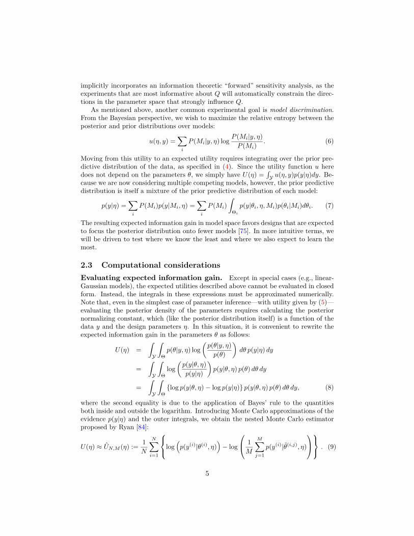
2.3 Computational considerationsEvaluating expected information gain. Except in special cases (e.g., linear-Gaussian models), the expected utilities described above cannot be evaluated in closedform. Instead, the integrals in these expressions must be approximated numerically.Note that, even in the simplest case of parameter inference—with utility given by (5)—evaluating the posterior density of the parameters requires calculating the posteriornormalizing constant, which (like the posterior distribution itself) is a function of thedata y and the design parameters ÷. In this situation, it is convenient to rewrite theexpected information gain in the parameters ◊ as follows:
where the second equality is due to the application of Bayes’ rule to the quantitiesboth inside and outside the logarithm. Introducing Monte Carlo approximations of theevidence p(y|÷) and the outer integrals, we obtain the nested Monte Carlo estimatorproposed by Ryan [84]:
U(÷) ¥ UN,M (÷) := 1N
Nÿ
i=1
Y]
[log1
p(y(i)|◊(i), ÷)
2≠ log
Q
a 1M
Mÿ
j=1
p(y(i)|◊(i,j)
, ÷)
R
b
Z^
\ . (9)
5
Here {◊
(i)} and {◊
(i,j)}, i = 1 . . . N , j = 1 . . . M , are independent samples from theprior p(◊), and each y
(i) is an independent sample from the likelihood p(y|◊(i), ÷), for
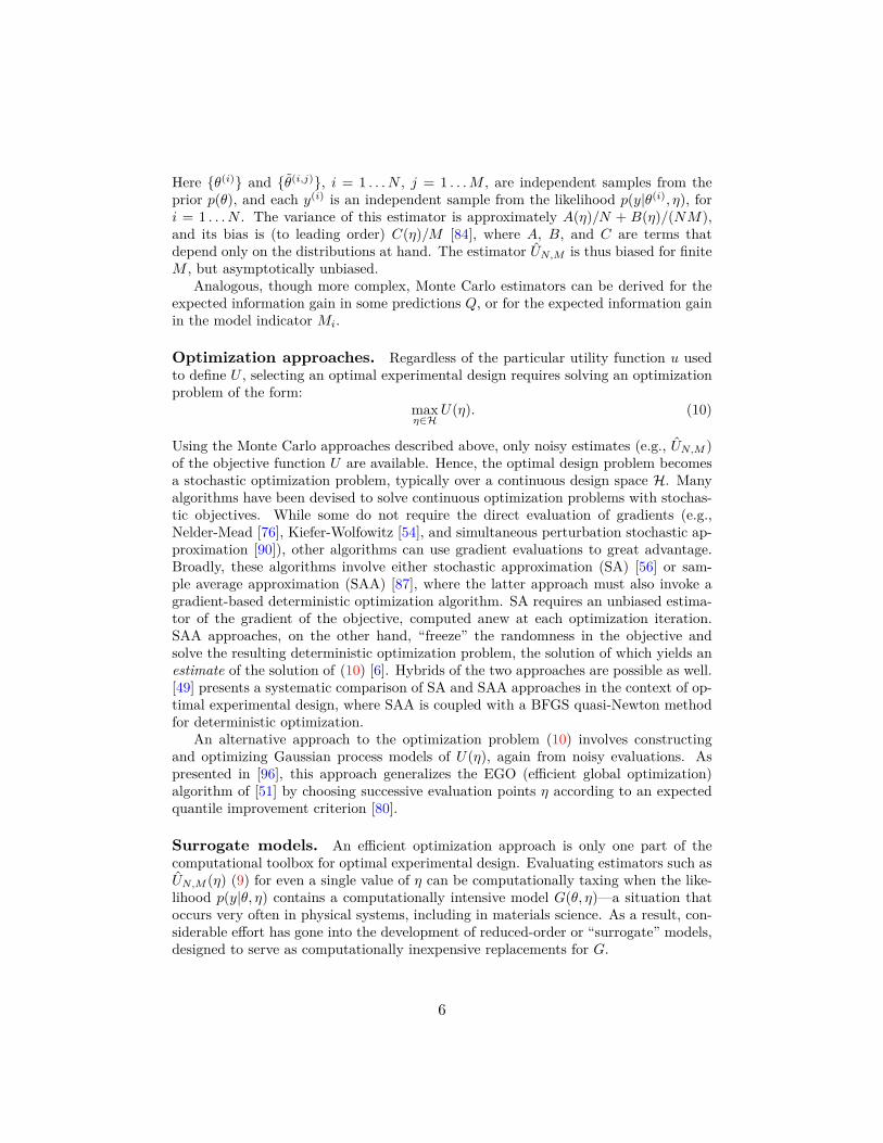
i = 1 . . . N . The variance of this estimator is approximately A(÷)/N + B(÷)/(NM),and its bias is (to leading order) C(÷)/M [84], where A, B, and C are terms thatdepend only on the distributions at hand. The estimator UN,M is thus biased for finiteM , but asymptotically unbiased.
Analogous, though more complex, Monte Carlo estimators can be derived for theexpected information gain in some predictions Q, or for the expected information gainin the model indicator Mi.
Optimization approaches. Regardless of the particular utility function u usedto define U , selecting an optimal experimental design requires solving an optimizationproblem of the form:
max÷œH
U(÷). (10)
Using the Monte Carlo approaches described above, only noisy estimates (e.g., UN,M )of the objective function U are available. Hence, the optimal design problem becomesa stochastic optimization problem, typically over a continuous design space H. Manyalgorithms have been devised to solve continuous optimization problems with stochas-tic objectives. While some do not require the direct evaluation of gradients (e.g.,Nelder-Mead [76], Kiefer-Wolfowitz [54], and simultaneous perturbation stochastic ap-proximation [90]), other algorithms can use gradient evaluations to great advantage.Broadly, these algorithms involve either stochastic approximation (SA) [56] or sam-ple average approximation (SAA) [87], where the latter approach must also invoke agradient-based deterministic optimization algorithm. SA requires an unbiased estima-tor of the gradient of the objective, computed anew at each optimization iteration.SAA approaches, on the other hand, “freeze” the randomness in the objective andsolve the resulting deterministic optimization problem, the solution of which yields anestimate of the solution of (10) [6]. Hybrids of the two approaches are possible as well.[49] presents a systematic comparison of SA and SAA approaches in the context of op-timal experimental design, where SAA is coupled with a BFGS quasi-Newton methodfor deterministic optimization.
An alternative approach to the optimization problem (10) involves constructingand optimizing Gaussian process models of U(÷), again from noisy evaluations. Aspresented in [96], this approach generalizes the EGO (e�cient global optimization)algorithm of [51] by choosing successive evaluation points ÷ according to an expectedquantile improvement criterion [80].
Surrogate models. An e�cient optimization approach is only one part of thecomputational toolbox for optimal experimental design. Evaluating estimators such asUN,M (÷) (9) for even a single value of ÷ can be computationally taxing when the like-lihood p(y|◊, ÷) contains a computationally intensive model G(◊, ÷)—a situation thatoccurs very often in physical systems, including in materials science. As a result, con-siderable e�ort has gone into the development of reduced-order or “surrogate” models,designed to serve as computationally inexpensive replacements for G.
6
Useful surrogate models can take many di�erent forms. [34] categorizes surrogatesinto three di�erent classes: data-fit models, reduced-order models, and hierarchicalmodels. Data-fit models are typically generated using interpolation or regression ofof the input-output relationship induced by the high-fidelity model G(◊, ÷), based onevaluations of G at selected input values (◊(i)
, ÷
(i)). This class includes polynomialchaos expansions that are constructed non-intrusively [41, 57, 100] and, more broadly,interpolation or pseudospectral approximation with standard basis functions on (adap-tive) sparse grids [24, 40, 101]. Gaussian process emulators [53, 99], widely used in thestatistics community, fall into this category as well. Indeed, the systematic and e�cientconstruction of data-fit surrogates, particularly for high-dimensional input spaces, hasbeen the focus of a vast body of work in computational mathematics and statisticsover the past decade. While many of these methods are used in forward uncertaintypropagation (e.g., the solution of PDEs with random input data), recent work [48]has employed sparse grid polynomial surrogates specifically for the case of optimalBayesian experimental design.
Reduced-order models are commonly derived using a projection framework; thatis, the governing equations of the forward model are projected onto a subspace of re-duced dimension. This reduced subspace is defined via a set of basis vectors, which,for general nonlinear problems, can be calculated via the proper orthogonal decompo-sition (POD) [47, 88, 81] or with reduced basis methods [77, 43]. For both approaches,the empirical basis is pre-constructed using full forward problem simulations or “snap-shots.” Systematic projection-based model reduction schemes for parameter-dependentmodels have also seen extensive development in recent years [17, 22]. To our knowl-edge, such reduction schemes have not yet been used for optimal experimental design,but in principle they are directly applicable.
Hierarchical surrogate models span a range of physics-based models of lower accu-racy and reduced computational cost. Hierarchical surrogates are derived from higher-fidelity models using approaches such as simplifying physics assumptions, coarser grids,alternative basis expansions, and looser residual tolerances. These approaches may notbe particularly systematic, in that their success and applicability are strongly problem-dependent, but they can be quite powerful in certain cases. One of the examples in thenext section will use a reduced order model derived from a combination of simplifyingphysics assumptions and fits to simulation data from a higher-fidelity model.
3 Examples of optimal experimental designIn this section, we present two examples of Bayesian experimental design in materials-related applications. The first illustrates experimental design for parameter estimationin a simple substrate-film model. This example also demonstrates the usefulness ofreduced-order models in accelerating the design process. The second example is con-cerned with experimental design for model selection. It will illustrate this process usingcompeting models of impurity precipitation at heterophase interfaces.
7
3.1 Film-substrate systems: design for parameter inferenceA classical application of Bayesian methods to physical modeling involves inferring theproperties of the interior of an object from observations of its surface, e.g., of the mantleor core of the Earth from observations at the Earth’s crust [16, 44]. In the contextof materials science, similar problems arise when observing the surface of a materialand trying to infer the subsurface properties. One example of such a problem involvesobserving a thin film deposited on a heterogeneous substrate. The heterogeneity of thesubstrate—e.g., in temperature [58], local chemistry [3], or topography [14]—inducessome corresponding heterogeneity in the film—e.g., melting [58], condensation [3], orbuckling [14]. The goal is to deduce information about the substrate from the behaviorof the film.
We have recently developed a convenient model for studying the inference of sub-strate properties from film behavior [2]. Figure 1 shows a film deposited on a substrate.Though the substrate is not directly observable, we would like to infer its propertiesfrom the behavior of the film deposited above. In the present example, we will use thissimple model to demonstrate aspects of Bayesian experimental design. Our objectivewill be to choose experiments that provide maximal information about a parameter ofinterest for a fixed number of allowed experiments.
3.1.1 Physical backgroundIn our model problem, the substrate is described by a non-uniform scalar field T (x, y)on a two-dimensional spatial domain, (x, y) œ � := [0, LD] ◊ [0, LD]. In other words,T (x, y) describes the variation of the substrate property T over a square domain.Realizations of the substrate are random, and hence we model T (x, y) as a zero-meanGaussian random field with a squared exponential covariance kernel [82]. One of thekey parameters of this covariance kernel is the characteristic length scale ¸s, whichdescribes the scale over which spatial variations in the random field occur. When ¸s islarge, realizations of the substrate field have a relatively coarse structure, while smallervalues of ¸s produce realizations with more fine-scale variation. The film deposited onthe substrate is a two-component mixture represented by an order parameter fieldc(x, y, t). The order parameter takes values in the range [≠1, 1], where c = ≠1 andc = 1 represent single-component phases and c = 0 represents a uniformly mixed phase.
The behavior of the film is modeled by the Cahn-Hilliard equation [18]:
ˆc
ˆt
= �3
ˆg
ˆc
≠ ‘
2�c
4, (11)
whereg (c, T (x, y)) = c
4
4 + T (x, y)c
2
2 (12)
is a substrate-dependent energy potential function. The two components of the filmseparate in regions of the substrate where T (x, y) < 0 and mix in regions whereT (x, y) > 0. Hence, the substrate field can be thought of as a di�erence from somecritical temperature, where temperatures above the critical value promote phase mix-ing while those below the critical value promote phase separation. The parameter ‘
8
Figure 1: A film deposited on top of a substrate. The substrate is not directly observable,but some of its properties may be inferred from the behavior of the film.
in (11) governs the thickness of the interface between separated phases. Films withlarger values of ‘ have thicker interfaces between their phase-separated regions thanfilms with lower values of ‘.
We model the time evolution of an initially uniform film c(x, y, t = 0) = 0 de-posited on a substrate by solving the Cahn-Hilliard equation using Eyre’s method fortime discretization [35]. We find that the order parameter field c converges to a staticconfiguration in the long time limit for any combination of ¸s and ‘. A detailed de-scription of the model implementation and analysis of the time-dependence of c is givenin [2]. For the purpose of the example presented here, it su�ces to know that the con-verged order parameter field has a characteristic length scale of its own, which we call�Œ.
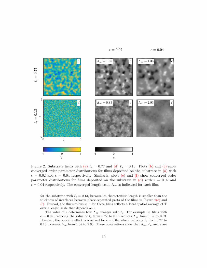
Figure 2 illustrates converged order parameter fields of films with two di�erentvalues of ‘ (‘ = 0.02 and ‘ = 0.04) deposited on substrates with two di�erent valuesof ¸s (¸s = 0.77 and ‘ = 0.13). For both substrates, we observe that increasing thevalue of ‘ increases the value of �Œ. Yet the behavior of the film on the two substratesis qualitatively di�erent. For the substrate with ¸s = 0.77, the thickness of interfacesbetween phase-separated parts of the film is su�ciently small for fluctuations in c to becorrelated with fluctuations in T . By contrast, no direct correlation of this sort exists
9
Figure 2: Substrate fields with (a) ¸s = 0.77 and (d) ¸s = 0.13. Plots (b) and (c) showconverged order parameter distributions for films deposited on the substrate in (a) with‘ = 0.02 and ‘ = 0.04 respectively. Similarly, plots (e) and (f) show converged orderparameter distributions for films deposited on the substrate in (d) with ‘ = 0.02 and‘ = 0.04 respectively. The converged length scale �Œ is indicated for each film.
for the substrate with ¸s = 0.13, because its characteristic length is smaller than thethickness of interfaces between phase-separated parts of the films in Figure 2(e) and(f). Instead, the fluctuations in c for these films reflects a local spatial average of T
over a length scale that depends on ‘.The value of ‘ determines how �Œ changes with ¸s. For example, in films with
‘ = 0.02, reducing the value of ¸s from 0.77 to 0.13 reduces �Œ from 1.05 to 0.83.However, the opposite e�ect is observed for ‘ = 0.04, where reducing ¸s from 0.77 to0.13 increases �Œ from 1.35 to 2.93. These observations show that �Œ, ¸s, and ‘ are
10
related, albeit in a non-trivial way.Our goal is to infer the substrate length scale ¸s from the value of �Œ of a film of
known ‘, deposited on the substrate. In this context, �Œ is the data obtained from anexperiment, ¸s is the value to be inferred, and ‘ is a parameter of the experiment thatwe control (e.g., by manipulating the chemical composition of the film). In previouswork, we showed how to perform this inference and how to improve it by performingmultiple measurements of �Œ using films with di�erent ‘ values [2]. In the experimentaldesign problem described here, we would like to choose optimal values of ‘ that leadto the most e�cient inference of ¸s.
For any given ¸s and ‘, �Œ may be obtained by solving the Cahn-Hilliard equationfor the time evolution of the film on the substrate. This calculation does not callfor extraordinary computational resources; indeed, it can be performed in roughly100 seconds on a modern workstation. In Bayesian experimental design, however,this calculation would have to be carried out many millions of times. The potentialcomputational e�ort of this approach is compounded by the stochasticity of T (x, y);to evaluate the likelihood function for any given value of ¸s, we must account for manypossible substrate field realizations. Therefore, to make optimal experimental designtractable, we construct a “reduced order model” (ROM) relating �Œ, ¸s, and ‘. Weuse a relation of the form
�Œ =reduced order model˙ ˝¸ ˚
f(‘, ¸s)¸ ˚˙ ˝deterministic term
+ “(‘, ¸s)¸ ˚˙ ˝random term
. (13)
The deterministic term captures the average response of the film/substrate system, andthe random term captures the inherent stochasticity of the film/substrate system andany systematic error in the deterministic term. The stochasticity of the film/substratesystem is due to the random nature of the substrate field and the initial condition ofthe Cahn-Hilliard equation, among other factors [2].
The proposed ROM can be simplified using the Buckingham Pi theorem [102]. Since‘, ¸s, and �Œ all have dimensions of length, we can form two Pi groups: (�Œ/‘) and(¸s/‘). The ROM may then be simplified to
�Œ‘
= F
3¸s
‘
4+ �
3¸s
‘
4. (14)
To obtain the form of F (¸s/‘) and �(¸s/‘), we carried out multiple runs of the Cahn-Hilliard model, with values of ¸s sampled over [0.1, 1] and values of ‘ sampled over[0.01, 0.1]. Figure 3(a) plots �Œ/‘ as a function of ¸s/‘, confirming that these quantitieslie on a single curve, on average. However, there is a spread about this curve as well.This is caused by the stochastic nature of the relation between �Œ/‘ and ¸s/‘, andjustifies the random term in the ROM. The exact forms of F (¸s/‘) and �(¸s/‘) arethen:
F
3¸s
‘
4= ¸s
‘
3a + b
(¸s/‘ ≠ 1)c
4(15)
�3
¸s
‘
4≥ N
30, ‡
2
3¸s
‘
44(16)
11
with parameters of the mean term F obtained by least squares fitting:
a = 1.05 b = 79.51 c = 1.54.
The dependence of ‡
2 on (¸s/‘) is captured nonparametrically using Gaussian processregression [82], as shown in Figure 3(b). Details of the derivation of the ROM can befound in [2].
!s/!101 102
!!/!
s
0
10
20
30
40
50
60
70
80
90
100
Data
ROM
±"
(a)
!s/!101 102
"2(!
s/!)
101
(b)
Figure 3: (a) A plot of �Œ/‘ against ¸s/‘. (b) A plot of the non-stationary variance of therandom term �(¸s/‘).
To perform inference, we use the Cahn-Hilliard model as a proxy for a physicalexperiment. We generate multiple realizations of substrates with the same value of ¸s.Then, using each substrate as an input, we run the Cahn-Hilliard model, which alsorequires ‘ as a parameter. Given one or more choices for ‘ and the values of �Œ thusobtained, we infer the value of ¸s using the ROM. Inference may be conducted usingone or multiple (�Œ, ‘) pairs.
To infer ¸s in a Bayesian setting, we need to calculate the likelihood p(�Œ, ‘). Thiscan be done using the ROM as follows:
p (�Œ|¸s, ‘) = 1Ô2fi‡(¸s/‘)
expA
≠ (�Œ/¸s ≠ F (¸s/‘))2
2‡
2(¸s/‘)
B. (17)
Since runs of the Cahn-Hilliard equation are conditionally independent given ¸s and ‘,the likelihood for multiple (�Œ, ‘) pairs can be found using the product rule
p (�Œ,1:n|¸s, ‘
1:n) =Ÿ
i
p (�Œ,i|¸s, ‘i) . (18)
12
Finally, the posterior density is calculated using Bayes’ rule
p(¸s|�Œ,1:n, ‘
1:n) = p(�Œ,1:n|¸s, ‘
1:n)p(¸s)sp(�Œ,1:n|¸s, ‘
1:n)p(¸s)d¸s. (19)
We use a truncated Je�reys prior [50] for ¸s
p(¸s) à ln(1/¸s), ¸s œ [0.1, 1]. (20)
The prior density is set to zero outside the range [0.1, 1]. This restriction is imposedfor reasons of computational convenience and may easily be relaxed.
The results of an iterative inference process that incorporates successive (�Œ, ‘)pairs are shown in Figure 4(a). Here, the true value of the substrate length scale (i.e.,the value used to generate the data) is ¸s = 0.4. Values of ‘ are selected by samplinguniformly in log-space over the interval [0.01, 0.1]. The probability density marked ‘0’(i.e., with zero data points) is the prior. The posterior probability density with onedata point (marked ‘1’) is bimodal, but the bimodality of the posterior vanishes withtwo or more data points. As additional (�Œ, ‘) pairs are introduced, the peak in theposterior moves towards the true value of ¸s = 0.4. Any number of point estimatesof ¸s may be calculated from the posterior, such as the mean, median, or mode, butthe posterior probability density itself gives a full characterization of the uncertaintyin ¸s. As an example, we have plotted in Figure 4(b) both the posterior variance (ameasure of uncertainty) and the absolute di�erence between the posterior mean andthe true value of ¸s (a measure of error) for di�erent numbers of data points. As moredata are used in the inference problem, both the posterior variance and the error inthe posterior mean decrease. Note that the ultimate convergence of the posterior meantowards the true value of ¸s, as the number of data points approaches infinity, is a moresubtle issue; it is related to the frequentist properties of this Bayesian estimator, herein the presence of model error. For a fuller discussion of this topic, see [2].
3.1.2 Bayesian experimental designThus far, we have described a model problem wherein the characteristic length scale ¸s
of a substrate is inferred from the behavior of films with known values of ‘, deposited onthe substrate. In the preceding calculations, we chose ‘ randomly from a distribution.Since ‘ is in fact an experimental parameter that we can control, this choice is equivalentto performing experiments at random. Now we would like to consider a more focusedexperimental campaign, choosing values of ‘ to maximize the information gained witheach experiment. In the language of Section 2, we will take our utility function u
to be the Kullback-Leibler (KL) divergence from the posterior to the prior (5). Theexpected utility (4) will represent expected information gain in the parameters ¸s. Toconnect the present problem to the general formulation of Section 2, note that �Œ isthe experimental data y, ¸s is the parameter ◊ to be inferred, and ‘ is the experimentalparameter ÷ over which we will optimize the expected utility.
The expected KL divergence from posterior to prior is estimated via the MonteCarlo estimator in (9). To perform the calculation, we need to be able to sample ¸
(i)s
and ˜(i,j)
s from the prior p(¸s), and �(i)Œ from the likelihood p(�Œ|¸(i)
s , ‘). The length
13
!s0.25 0.5 0.75 1
p(! s|!
!,!)
0
5
10
15
0
1
8
4
2
(a)
error in posterior mean10-2 10-1 100
posterior
varian
ce
10-5
10-4
10-3
10-2
10-1
24
8
16
32
64
(b)
Figure 4: (a) Posterior probability densities for di�erent numbers of (�Œ, ‘) pairs. Withthe inclusion of ever more data, uncertainty in the posterior on ¸s decreases steadily. (b)Posterior variance and error in posterior mean for di�erent numbers of (�Œ, ‘) pairs. Botherror and variance decrease with increasing numbers of data points.
scales ¸s can be sampled from the truncated Je�reys prior using a standard inverseCDF transformation [83]. The observation �Œ is Gaussian given ‘ and ¸s, and can besampled by evaluating (14) with distributional information given in (15)–(16).
We will use this formulation to design an optimal experiment consisting of twomeasurements. In other words, two films with independently controlled values of ‘
will be deposited on substrates with the same value of ¸s, and the two values of �Œgenerated will be used for inference. The values of ‘ will be restricted to the designrange [0.01, 0.095]. As before, this restriction is not essential and is easily relaxed.Figure 10 shows the resulting Monte Carlo estimates of expected information gainU(‘
1
, ‘
2
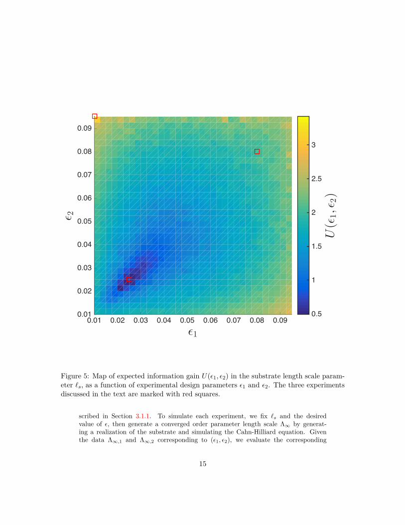
).Because the ordering of the experiments is immaterial, the map of the expected in-
formation gain is symmetric about the ‘
1
= ‘
2
line, aside from Monte Carlo estimationerror. We draw attention to three points marked by squares in Figure 10. The first isat (‘
1
, ‘
2
) = (0.025, 0.025), where U(‘1
, ‘
2
) = 0.49; it is near the minimum of the ex-pected utility function. This point corresponds to the least useful pair of experiments.The second is at (‘
1
, ‘
2
) = (0.01, 0.095), with U(‘1
, ‘
2
) = 2.9; it is the maximum of theexpected utility map and is expected to yield the most informative experiments. Thepoint (‘
1
, ‘
2
) = (0.08, 0.08), where U(‘1
, ‘
2
) = 2.0, lies midway between these extremes:it is expected to be more informative than the first design but less informative thanthe second.
To illustrate how the three (‘1
, ‘
2
) pairs highlighted above yield di�erent expectedutilities, we carry out the corresponding inferences of ¸s following the procedure de-
14
!10.01 0.02 0.03 0.04 0.05 0.06 0.07 0.08 0.09
! 2
0.01
0.02
0.03
0.04
0.05
0.06
0.07
0.08
0.09
U(!
1,!
2)
0.5
1
1.5
2
2.5
3
Figure 5: Map of expected information gain U(‘1, ‘2) in the substrate length scale param-eter ¸s, as a function of experimental design parameters ‘1 and ‘2. The three experimentsdiscussed in the text are marked with red squares.
scribed in Section 3.1.1. To simulate each experiment, we fix ¸s and the desiredvalue of ‘, then generate a converged order parameter length scale �Œ by generat-ing a realization of the substrate and simulating the Cahn-Hilliard equation. Giventhe data �Œ,1 and �Œ,2 corresponding to (‘
1
, ‘
2
), we evaluate the corresponding
15
posterior density and calculate the actual KL divergence from posterior to prior,DKL (p(¸s|�Œ,1:2
, ‘
1:2
)Îp(¸s)). The results of these three experiments are summa-rized in Figure 6(a). As expected, the second experiment, performed at (‘
1
, ‘
2
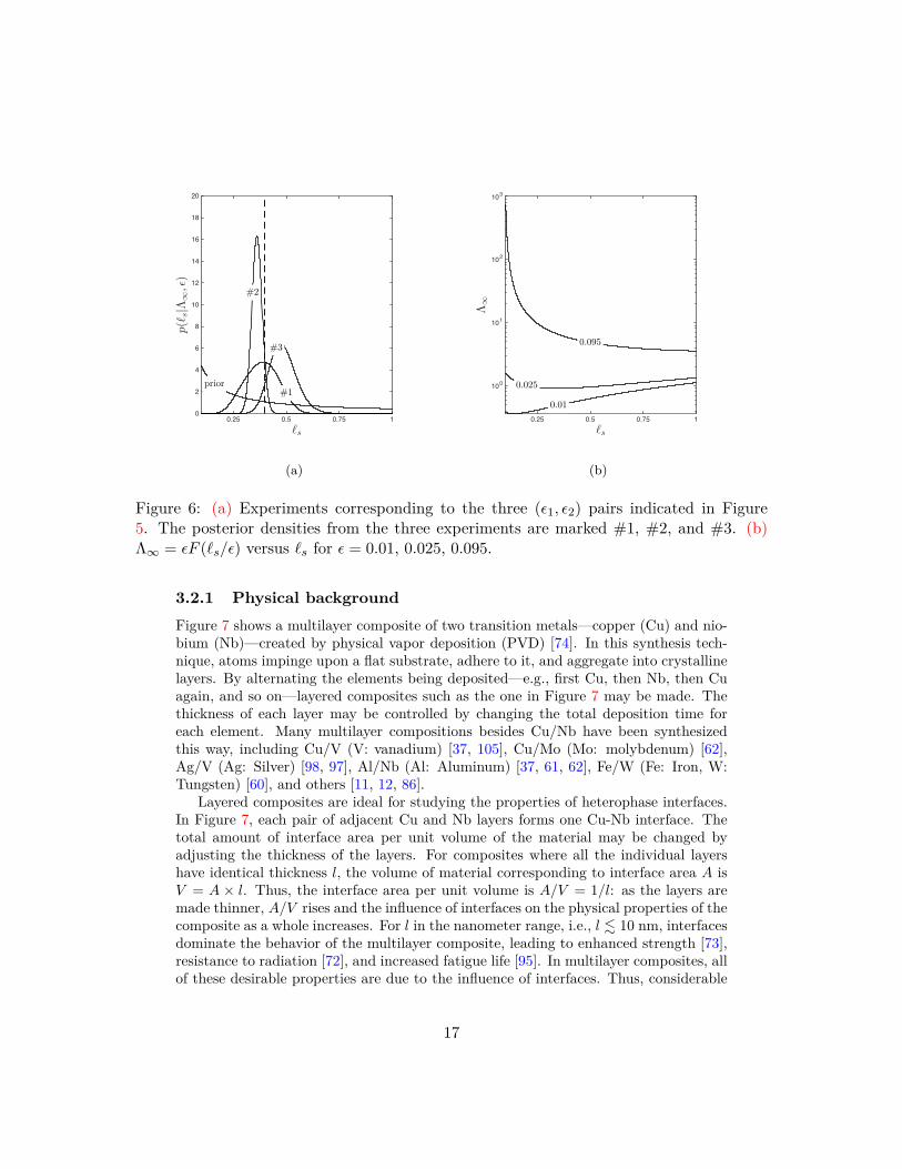
) =(0.01, 0.095) is the most informative, and has a large information gain of DKL = 2.10nats.1 The first experiment is the least informative, with a small information gain ofDKL = 0.99 nats. The third experiment, with DKL = 1.44 nats, lies in between. Theactual values of DKL are di�erent from their expected values because the expectedinformation gains are calculated by averaging over all possible prior values of ¸s andall possible experimental outcomes, whereas the actual values are calculated only forparticular ¸s and �Œ values, given ‘. However, the values of DKL follow the sametrend as their expectations.
To better understand why these experiments produce di�erent values of the infor-mation gain, Figure 6(b) plots �Œ = ‘F (¸s/‘) as a function of ¸s for ‘ = 0.01, 0.025,and 0.095. We observe that �Œ is not very sensitive to variations in ¸s for ‘ = 0.025.This explains why an experiment with (‘
1
, ‘
2
) = (0.025, 0.025) is not particularly in-formative. On the other hand, �Œ is sensitive to variations in ¸s for ‘ = 0.095 and‘ = 0.01. Additionally, �Œ is a decreasing function of ¸s for ‘ = 0.095, and an increas-ing function for ‘ = 0.01. The complementarity of these trends makes the experiment(‘
1
, ‘
2
) = (0.01, 0.095) especially useful.We can also compare the optimal experiment to the random experiments shown in
Figure 4. The information gained in the optimal experiment (DKL = 2.10 nats), withtwo values of ‘, is comparable to the information gained from the experiment with eightrandomly selected values of ‘ (DKL = 2.29 nats). Hence by using optimal Bayesianexperimental design in this example, we are able to reduce the experimental e�ort overa random strategy by roughly a factor of four! This reduction is especially valuablewhen experiments are di�cult or expensive to conduct.
3.2 Heterophase interfaces: design for model discriminationAs noted in Section 2.1, experiments often yield data that may be explained by mul-tiple models. Additional measurements may then be required to determine which ofmany possible models is best supported by the data. In such situations, it is desirableto determine which further experiments are likely to distinguish between alternativemodels most e�ciently. Naturally, this guidance is needed before the additional workis actually carried out. Determining which experiments are most informative for dis-tinguishing between alternative models is the goal of Bayesian experimental design formodel selection [63, 75]. This capability is especially useful when the experiments arevery resource-intensive and brute force data acquisition over a wide parameter rangeis not feasible. This section will illustrate Bayesian experimental design for model se-lection on an example taken from investigations of heterophase interfaces in layeredmetal composites.
1A nat is a unit of information, analogous to a bit, but with a natural logarithm rather than a base two
logarithm in (5).
16
!s0.25 0.5 0.75 1
p(! s|!
!,!)
0
2
4
6
8
10
12
14
16
18
20
prior#1
#2
#3
(a)
!s0.25 0.5 0.75 1
!!
100
101
102
103
0.025
0.01
0.095
(b)
Figure 6: (a) Experiments corresponding to the three (‘1, ‘2) pairs indicated in Figure5. The posterior densities from the three experiments are marked #1, #2, and #3. (b)�Œ = ‘F (¸s/‘) versus ¸s for ‘ = 0.01, 0.025, 0.095.
3.2.1 Physical backgroundFigure 7 shows a multilayer composite of two transition metals—copper (Cu) and nio-bium (Nb)—created by physical vapor deposition (PVD) [74]. In this synthesis tech-nique, atoms impinge upon a flat substrate, adhere to it, and aggregate into crystallinelayers. By alternating the elements being deposited—e.g., first Cu, then Nb, then Cuagain, and so on—layered composites such as the one in Figure 7 may be made. Thethickness of each layer may be controlled by changing the total deposition time foreach element. Many multilayer compositions besides Cu/Nb have been synthesizedthis way, including Cu/V (V: vanadium) [37, 105], Cu/Mo (Mo: molybdenum) [62],Ag/V (Ag: Silver) [98, 97], Al/Nb (Al: Aluminum) [37, 61, 62], Fe/W (Fe: Iron, W:Tungsten) [60], and others [11, 12, 86].
Layered composites are ideal for studying the properties of heterophase interfaces.In Figure 7, each pair of adjacent Cu and Nb layers forms one Cu-Nb interface. Thetotal amount of interface area per unit volume of the material may be changed byadjusting the thickness of the layers. For composites where all the individual layershave identical thickness l, the volume of material corresponding to interface area A isV = A ◊ l. Thus, the interface area per unit volume is A/V = 1/l: as the layers aremade thinner, A/V rises and the influence of interfaces on the physical properties of thecomposite as a whole increases. For l in the nanometer range, i.e., l . 10 nm, interfacesdominate the behavior of the multilayer composite, leading to enhanced strength [73],resistance to radiation [72], and increased fatigue life [95]. In multilayer composites, allof these desirable properties are due to the influence of interfaces. Thus, considerable
17
e�ort continues to be invested into elucidating the structure and properties of individualinterfaces [71, 19, 10].
The present example will consider the relationship between the structure of metal-metal heterophase interfaces and trapping of helium (He) impurities. Implanted He is amajor concern for the performance of materials in nuclear energy applications [92, 106].Trapping and stable storage of these impurities at interfaces is one way of mitigatingthe deleterious e�ects of implanted He [78, 32]. The influence of interfaces on Hemay be clearly seen in multilayer composites. Experiments carried out on Cu-Nb [29],Cu-Mo [62], and Cu-V [38] multilayers synthesized by PVD show that implanted Heis preferentially trapped at the interfaces. Moreover, not all interfaces are equallye�ective at trapping He: the maximum concentration c of interfacial He—expressed asthe number of He atoms per unit interface area—that may be trapped at an interfacebefore detectable He precipitates form di�ers from interface to interface [32].
Figure 8 plots c for Cu-Nb, Cu-Mo, and Cu-V interfaces as a function of one pa-rameter: the interface “misfit” m. Cu, Nb, Mo, and V all have cubic crystal structures:Cu is face-centered cubic (fcc) while Nb, Mo, and V are body-centered cubic (bcc).Thus, all three composites used in Figure 8 are made up of alternating fcc (Cu) andbcc (Nb, Mo, or V) layers. The edge length of a single cubic unit cell in fcc or bcccrystals is the lattice parameter, a
fcc
or a
bcc
. The misfit m is defined as m = a
bcc
/a
fcc
.Intuitively, m measures the mismatch in inter-atomic spacing in the adjacent crystalsthat make up an interface.
According to Figure 8, the ability of interfaces to trap He, as measured by c, dependson the misfit: c = c(m). A simple model that may be proposed based on this data isthat the relationship between c and m is linear: c = –
0
+ –
1
m. Indeed, a linear fitrepresents the available data reasonably well. Its most apparent drawback is that itpredicts negative c values for m . 0.83. Thus, a better model might be c = –|m≠m
0
|.This model predicts that c drops to zero as m decreases to m
0
and begins to riseagain as m is further reduced below m
0
. Physically, this model may be rationalized bystating that at some special value of misfit, m
0
, the atomic matching between adjacentlayers is especially good, leading to few sites at the interface where He impurities maybe trapped. As m departs from m
0
in either direction, the atomic matching becomesworse, giving rise to more He trapping sites and therefore higher c.
The structure of fcc/bcc interfaces—including the degree of atomic matching—may be investigated in detail by constructing atomic-level models [33, 30]. Figure9 shows such a model of the terminal atomic planes of Cu and Nb found at PVDCu-Nb interfaces. The pattern of overlapping atoms from the two planes containssites where a Cu atom is nearly on top of a Nb atom. Such sites are thought to bepreferential locations for trapping of He impurities [52]. They arise from the geometricalinterference of the overlapping atomic arrangements in the adjacent crystalline layersand, in that sense, may be viewed as analogous to features in a Moiré pattern.
The density and distribution of He trapping sites of the type shown in Figure 9may be computed directly for any given fcc/bcc interface as a function of the geometryof the interface using the well-known O-lattice theory [13]. In PVD Cu/Nb, Cu/Mo,and Cu/V composites, the relative orientation of the adjacent crystals is identical.Thus, di�erences in the geometry Cu-Nb, Cu-Mo, and Cu-V interfaces arise solelyfrom di�erences in the lattice parameters of the adjacent crystals, as described by the
18
misfit parameter, m. The areal density of He trapping sites for these interfaces istherefore only a function of m and may be written as
f(m) =--(4m ≠ 3)(
Ô3m ≠ Ô
2)--
3a
2
Cu
m
2
. (21)
Using this expression, we propose a second model for the dependence of c on m, namely:c = —f(m). Here, the proportionality constant — determines the number of He atomsthat may be trapped at a single site of the type illustrated in Figure 9. The bestfit for this second model is plotted in Figure 8. Both this model and the previouslydescribed linear model fit the available experimental data reasonably well. Moreover,both predict c values of zero for m ¥ 0.82–0.83. However, unlike the linear model,c = —f(m) predicts that c is also zero at m ¥ 0.75.
We wish to determine what additional experimental data will help distinguish be-tween the two models described above. However, since measuring even a single valueof c requires considerable resources, our goal is to limit the additional data to just one(c, m) pair. In an experiment, we may select m by choosing to synthesize a fcc/bccmultilayer composite of specific composition. In other words, we control m. However,we do not know c in advance. In this context, our goal is to determine what one valueof m is most likely to distinguish between the two models, regardless of the c valueactually found in the subsequent experiment. In the following section, we will applyBayesian experimental design to address this challenge. In addition to the two modelsdescribed above, we will also consider a third model encapsulating the hypothesis thatc does not depend on m at all: c = “ = constant.
Figure 7: A Cu-Nb multilayer composite synthesized by PVD [31].
19
Figure 8: Maximum interfacial He impurity concentration, c, plotted as a function of misfit,m.
3.2.2 Bayesian experimental design for model selectionAs described in Section 2, the goal of experimental design is to maximize the expec-tation of some measure of information. In the present example, we will maximize theexpected KL divergence, as applied to model discrimination, described in (6) and (7).In this context, m is the experimental parameter ÷ that we control; c is the observeddata y; M
1
, M
2
, and M
3
are the competing models; (–, m
0
) are the parameters ◊
1
ofmodel M
1
; — is the parameter ◊
2
of model M
2
; and “ is the parameter ◊
3
of model M
3
.The expected KL divergence can be computed by combining (6) and (7); this re-
quires knowing both the prior p(Mi) and the posterior p(Mi|c, m) for each model. Wewe use a flat or “indi�erence” prior over models, p(Mi) = 1/3. The posterior modelprobabilities are calculated from Bayes rule as given in (2). Evaluating Bayes’ rulein this setting requires that we calculate the marginal likelihood for each model andproposed experiment, p(c|Mi, m), as shown in (3). We now detail this procedure.
The previous section identified three models connecting c and m. They are:
M
1
: c = –|m ≠ m
0
| + ‘
1
(22)M
2
: c = —f(m) + ‘
2
(23)M
3
: c = “ + ‘
3
(24)
where ‘i ≥ N(0, ‡
2
‘ ). In addition to specifying the functional form of each model,each expression above also contains an additive noise term ‘i. This term is a randomvariable that describes uncertainty in the measured c, i.e., due to the observational
20
Figure 9: Left: a Cu-Nb bilayer. Right: the terminal Cu and Nb planes that meet at theCu-Nb interface. He trapping occurs at sites where a Cu atom is nearly on top of a Nbatom. One such site is shown with the dashed circle.
process itself. For simplicity, we assume the observational error variance ‡
2
‘ to beknown. The model parameters –, m
0
, —, and “ are endowed with priors that reflectour state of knowledge after performing the three experiments shown in Figure 8,before beginning the current experimental design problem. These priors are taken tobe Gaussian. In other words, we suppose that they are the result of Bayesian linearregression with Gaussian priors or improper uniform priors; the posterior followingthe three previous experiments becomes the prior for the current experimental designproblem. We denote the current prior means by –, m
0
, —, and “, and the current priorstandard deviations as ‡–, ‡m0 , ‡— , and ‡“ .
Given these assumptions, we can express the probability density of the observationc for each parameterized model as:
p(c|m, –, m
0
, M
1
) = 1Ô2fi‡‘
exp3
≠ (c ≠ –|m ≠ m
0
|)2
2‡
2
‘
4(25)
p(c|m, —, M
2
) = 1Ô2fi‡‘
exp3
≠ (c ≠ —f(m))2
2‡
2
‘
4(26)
p(c|m, “, M
3
) = 1Ô2fi‡‘
exp3
≠ (c ≠ “)2
2‡
2
‘
4. (27)
Each of these densities is normal with mean given by the model and variance ‡
2
‘ .For fixed m and c, these densities can be viewed as the likelihood functions for thecorresponding model parameters, i.e., – and m
0
for model 1, — for model 2, and “
for model 3. To obtain the marginal likelihoods p(c|m, Mi), we marginalize out these
21
parametric dependencies as follows:
p(c|m, M
1
) =⁄ Œ
≠Œp(c|m, –, m
0
, M
1
)p(–)p(m0
) d– dm
0
(28)
p(c|m, M
2
) =⁄ Œ
≠Œp(c|m, —, M
2
)p(—) d— (29)
p(c|m, M
3
) =⁄ Œ
≠Œp(c|m, “, M
1
)p(“) d“ (30)
Here, p(–), p(m0
), p(—), and p(“) denote the Gaussian prior probability densitiesdescribed above, e.g.,
p(–) = 1Ô2fi‡–
exp3
≠ (– ≠ –)2
2‡
2
–
4, etc. (31)
In the expressions for p(c|m, Mi), integration over –, —, and “ can be performed ana-lytically, e.g.,
p(c|m, M
2
) = 1
‡—‡‘
Ú2fi‡2
—+ 2fif(m)
2
‡2‘
expA
≠ (c ≠ —f(m))2
2(f(m)2
‡
2
— + ‡
2
‘ )
B. (32)
The integral over m
0
in the expression for p(c|m, M
1
) must be found numerically, how-ever. In the present example, this integral is easily computed using standard numericalquadrature. If the integral had been too high dimensional, however, then a MonteCarlo scheme might be used instead [83]. We carry out these calculations using priorparameters listed in Table 1. The experimental uncertainty was set to ‡‘ = 2.5/nm2,following [29].
To calculate the expected information gain U in the model indicator, as a functionof the m value for a single additional experiment, we first substitute the prior andposterior model probabilities calculated above into (6). Then we take the expectationof this utility over the prior predictive distribution, as in (7), by integrating over thedata c. More explicitly, we calculate:
U(m) =⁄
u(m, c)p(c|m) dc, (33)
where the utility is
u(m, c) =3ÿ
i=1
P (Mi|c, m) log P (Mi|c, m)P (Mi)
,
and the design-dependent prior predictive probability density is
p(c|m) =3ÿ
i=1
P (Mi)p(c|m, Mi).
22
The integral in (33) formally is taken over (≠Œ, Œ), since this is the range of theprior predictive. Negative values of c are not physical, of course, but they are exceed-ingly rare: the mean predictions of models 1 and 2 are necessarily positive, and theGaussian prior on “ in model 3 is almost entirely supported above zero. The Gaussianmeasurement noise ‘ can also lead to negative c values, but it too has a relatively smallvariance.
Model Parameter Standard DeviationM1 – ¥ 94/nm2
‡– ¥ 0.49/nm2
m0 ¥ 0.83 ‡m0 ¥ 0.62M2 — ¥ 26/nm2
‡— ¥ 4.2/nm2
M3 “ ¥ 4.5/nm2‡“ = 2.0/nm2
Table 1: Prior model parameters.
Figure 10 plots U(m) computed using all three models. For comparison, the figurealso shows U(m) found using only models 1 and 2, i.e., excluding the constant modelc = “. Values of m that maximize U(m) are the best choices for an experiment todistinguish between models. When all three models are considered, U(m) is greatestfor high misfit, i.e., m ¥ 0.95. By contrast, when only models 1 and 2 are considered,U(m) is least in the high m limit. The reason for this di�erence is clear from comparingFigure 10 with Figure 8: models 1 and 2 predict comparable c at high m while model3 predicts a markedly lower c. Thus, when all three models are considered, the valueof U(m) is high for m ¥ 0.95 because a measurement at that m value makes it possibleto distinguish models 1 and 2 from model 3. By contrast, when only models 1 and 2are considered, U(m) is least at high m because a measurement in that m range haslimited value for distinguishing between models 1 and 2.
Putting aside model 3, U(m) predicts greatest utility for an experiment carried outin the range 0.74 < m < 0.84, i.e., in the vicinity of the minima of function f(m). Tounderstand the reason for the significance of this m range, it is important to realizethat the plots in Figure 8 only show a single realization of models 1 and 2, namely thosecorresponding to – = –, m
0
= m
0
, and — = — (the prior means on the parameters).Since we assume that –, m
0
, and — are normally distributed, many other realizationsof these models are possible. Figure 11 shows 100 di�erent realizations of models 1and 2 obtained by drawing –, m
0
, and — at random from their prior distributions.Figure 11 makes clear an important distinction between models 1 and 2 that is not
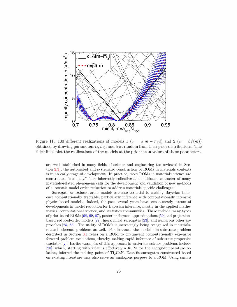
apparent in Figure 8: model 1 exhibits an extreme sensitivity to its fitting parameterswithin the range of uncertainty of those parameters. In particular, the minimum inc predicted by model 1 may occur at many di�erent m values. By contrast, model2 is relatively less sensitive to its fitting parameters, especially for 0.74 < m . 0.84.Unlike model 1, the locations of its minima are fixed. Thus, measuring a low c valuefor 0.74 < m . 0.84 has the potential to exclude a large number of realizations ofmodel 1, while measuring a high c value in that range essentially excludes model 2.Bayesian methods naturally capture this subtle aspect of experimental design withoutany special prior analysis of the competing models.
23
Figure 10: Expected information gain for model discrimination U(m).
4 OutlookThe examples presented here demonstrate how the formalism of optimal Bayesian ex-perimental design, coupled with information theoretic objectives, can be adapted todi�erent questions of optimal data collection in materials science. In one example,we seek the best pair of experiments for inferring the parameters of a given model.In another example, we seek the single experiment that can best distinguish betweencompeting models, where each model has a distinct form and a distinct set of un-certain parameters. Though simple, these examples also demonstrate the use of keycomputational and analytical tools, including the Monte Carlo estimation of expectedinformation gain (in the nonlinear and non-Gaussian setting of our first example) andthe use of reduced-order models (also in the first example).
Reduced order models (ROMs) are increasingly being recognized as crucial to mate-rials science, especially computational materials design [39, 70, 94, 104]. The reason fortheir utility is clear: strictly speaking, the complete set of degrees of freedom describinga material is the complete set of positions and types of all its constituent atoms. Thisset defines a design space far too vast to explore. Even if mesoscale entities such ascrystal defects (e.g., dislocations [45] or interfaces [91]) or microstructure [1] are usedto define the degrees of freedom for design, the resulting design space may neverthelessremain too vast to examine comprehensively.
Therefore, it is crucial to identify only those degrees of freedom that significantlya�ect properties of interest (e.g., those a�ecting performance metrics in a design) andcreate a ROM to connect the two. Yet while formal methods of model order reduction
24
Figure 11: 100 di�erent realizations of models 1 (c = –|m ≠ m0|) and 2 (c = —f(m))obtained by drawing parameters –, m0, and — at random from their prior distributions. Thethick lines plot the realizations of the models at the prior mean values of these parameters.
are well established in many fields of science and engineering (as reviewed in Sec-tion 2.3), the automated and systematic construction of ROMs in materials contextsis in an early stage of development. In practice, most ROMs in materials science areconstructed “manually.” The inherently collective and multiscale character of manymaterials-related phenomena calls for the development and validation of new methodsof automatic model order reduction to address materials-specific challenges.
Surrogate or reduced-order models are also essential to making Bayesian infer-ence computationally tractable, particularly inference with computationally intensivephysics-based models. Indeed, the past several years have seen a steady stream ofdevelopments in model reduction for Bayesian inference, mostly in the applied mathe-matics, computational science, and statistics communities. These include many typesof prior-based ROMs [68, 69, 67], posterior-focused approximations [59] and projection-based reduced-order models [27], hierarchical surrogates [23], and numerous other ap-proaches [25, 85]. The utility of ROMs is increasingly being recognized in materials-related inference problems as well. For instance, the model film-substrate problemdescribed in Section 3.1 relies on a ROM to circumvent computationally expensiveforward problem evaluations, thereby making rapid inference of substrate propertiestractable [2]. Earlier examples of this approach in materials science problems include[28], which, starting with what is e�ectively a ROM for the energy-temperature re-lation, inferred the melting point of Ti
2
GaN. Data-fit surrogates constructed basedon existing literature may also serve an analogous purpose to a ROM. Using such a
25
surrogate, [103] modeled the creep rupture life of Ni-base superalloys.Similar to reduced-order modeling, the usefulness of Bayesian approaches is now
becoming better recognized within the materials community. They can be applied toparameter inference and model inference, as demonstrated here, but also to problemsinvolving prediction under uncertainty. For example, [55] used Bayesian inference toassess the uncertainty of cluster expansion methods for computing the internal energiesof alloys. These authors point out that cluster expansions are also a kind of surrogatemodel—i.e., a ROM—and that uncertainty quantification should, among other goals,assess how well the surrogate reproduces the output of a more computationally expen-sive reference model.
Despite growing interest in Bayesian methods within the materials community,there are fewer examples of their application to experimental design. An early (yet veryrecent) e�ort is [4], which applies information-theoretic criteria and Bayesian methodsto stress-strain response and texture evolution in polycrystalline solids. Neverthe-less, opportunities for expanded application of optimal Bayesian experimental designabound in materials-related work. In particular, detailed and resource-intensive exper-iments such as those described in Section 3.2 are poised to benefit from it immensely.One potential hurdle to widespread adoption is the up-front investment of e�ort cur-rently needed to understand and implement the associated mathematical formalism.Thus, expanded availability of user-friendly, well-documented, and multi-functionalsoftware [79] is likely to accelerate the adoption and integration of Bayesian experi-mental design into mainstream materials research.
Finally, we emphasize that optimal experimental design itself—not limited to thematerials science context—is the topic of much current research. This research focuseson both formulational issues and on computational methodology. Examples of thelatter include developing reduced-order or multi-fidelity models tailored to the needsof stochastic optimization, or devising more e�cient estimators of expected informa-tion gain, using importance sampling, high-dimensional kernel density estimators, andother approaches. An interesting foundational challenge, on the other hand, involvesunderstanding and accounting for model error or misspecification in optimal design. Ifthe model relating parameters of interest to experimental observables is incomplete orunder-resolved, how useful—or close to optimal—are the experiments designed accord-ing to this relationship? When a convergent sequence of models of di�ering fidelityis available (as in the ROM setting), then this question is more tractable. But if allavailable models are inadequate, many questions remain open. One promising ap-proach to this challenge uses nonparametric statistical models, perhaps formulated ina hierarchical Bayesian manner, to account for interactions and inputs missing fromthe current model of the experiment. Sequential experimental design is also usefulin this context, as successive batches of experiments can help uncover the unmodeledmismatch between a model and physical reality.
Sequential experimental design is useful much more broadly as well. Recall thatin all the examples of this chapter, we designed a single batch of experiments all-at-once: even if the batch contained multiple experiments, we chose the design parametersbefore performing any of the experiments. Sequential design, in contrast, allows in-formation from each experiment to influence the design of the next. The most widelyused sequential approaches are greedy, where one designs the next batch of experi-
26
ments as if it were the final batch—using the current state of knowledge as the priordistribution, with design criteria similar to those used here. But greedy approaches aresub-optimal in general, as they do not account for the information to be gained fromfuture experiments. An optimal approach can instead be obtained by formulating se-quential experimental design as a problem of dynamic programming [9, 20, 7]. Makingthis dynamic programming approach computationally tractable, outside of specializedsettings, remains a significant challenge.
References[1] B. L. Adams, S. R. Kalidindi, and D. T. Fullwood, Microstructure sensi-
tive design for performance optimization, Butterworth-Heinemann, 2012.[2] R. Aggarwal, M. Demkowicz, and Y. Marzouk, Bayesian inference of
substrate properties from film behavior, Modelling and Simulation in MaterialsScience and Engineering, 23 (2015), p. 015009.
[3] J. Aizenberg, A. Black, and G. Whitesides, Controlling local disorder inself-assembled monolayers by patterning the topography of their metallic supports,Nature, 394 (1998), pp. 868–871.
[4] S. Atamturktur, J. Hegenderfer, B. Williams, and C. Unal, Selec-tion criterion based on an exploration-exploitation approach for optimal designof experiments, Journal of Engineering Mechanics, 141 (2014).
[5] A. C. Atkinson and A. N. Donev, Optimum Experimental Designs, OxfordStatistical Science Series, Oxford University Press, 1992.
[6] G. Bayraksan and D. P. Morton, Assessing solution quality in stochasticprograms via sampling, INFORMS Tutorials in Operations Research, 5 (2009),pp. 102–122.
[7] I. Ben-Gal and M. Caramanis, Sequential doe via dynamic programming, IIETransactions, 34 (2002), pp. 1087–1100.
[8] J. Berger and L. Pericchi, Objective Bayesian methods for model selection:introduction and comparison, Model Selection (P.Lahiri, editor), IMS LectureNotes – Monograph Series, 38 (2001), pp. 135–207.
[9] D. P. Bertsekas, Dynamic Programming and Optimal Control, Athena Scien-tific, 3rd ed., 2007.
[10] I. Beyerlein, M. Demkowicz, A. Misra, and B. Uberuaga, Defect-interface interactions, Progress in Materials Science, (2015).
[11] D. Bhattacharyya, N. Mara, P. Dickerson, R. Hoagland, andA. Misra, Transmission electron microscopy study of the deformation behav-ior of cu/nb and cu/ni nanoscale multilayers during nanoindentation, Journal ofMaterials Research, 24 (2009), pp. 1291–1302.
[12] , Compressive flow behavior of al–tin multilayers at nanometer scale layerthickness, Acta Materialia, 59 (2011), pp. 3804–3816.
[13] W. Bollmann, Crystal defects and crystalline interfaces, Springer, 1970.
27
[14] N. Bowden, S. Brittain, A. Evans, J. Hutchinson, and G. Whitesides,Spontaneous formation of ordered structures in thin films of metals supported onan elastomeric polymer, Nature, 393 (1998), pp. 146–149.
[15] G. E. P. Box and H. L. Lucas, Design of experiments in non-linear situations,Biometrika, 46 (1959), pp. 77–90.
[16] T. Bui-Thanh, O. Ghattas, J. Martin, and G. Stadler, A computa-tional framework for infinite-dimensional bayesian inverse problems part i: Thelinearized case, with application to global seismic inversion, SIAM Journal onScientific Computing, 35 (2013), pp. A2494–A2523.
[17] T. Bui-Thanh, K. Willcox, and O. Ghattas, Model reduction for large-scale systems with high-dimensional parametric input space, SIAM Journal onScientific Computing, 30 (2008), pp. 3270–3288.
[18] J. Cahn and J. Hilliard, Free energy of a nonuniform system. i. interfacialfree energy, J. Chem. Phys, 28 (1958), pp. 258–267.
[19] P. R. Cantwell, M. Tang, S. J. Dillon, J. Luo, G. S. Rohrer, and M. P.Harmer, Grain boundary complexions, Acta Materialia, 62 (2014), pp. 1–48.
[20] B. P. Carlin, J. B. Kadane, and A. E. Gelfand, Approaches for optimalsequential decision analysis in clinical trials, Biometrics, (1998), pp. 964–975.
[21] K. Chaloner and I. Verdinelli, Bayesian experimental design: A review,Statistical Science, 10 (1995), pp. 273–304.
[22] S. Chaturantabut and D. C. Sorensen, Nonlinear model reduction via dis-crete empirical interpolation, SIAM Journal on Scientific Computing, 32 (2010),pp. 2737–2764.
[23] J. A. Christen and C. Fox, MCMC using an approximation, Journal of Com-putational and Graphical statistics, 14 (2005), pp. 795–810.
[24] P. Conrad and Y. M. Marzouk, Adaptive Smolyak pseudospectral approxi-mations, SIAM Journal on Scientific Computing, 35 (2013), pp. A2643–A2670.
[25] P. Conrad, Y. M. Marzouk, N. Pillai, and A. Smith, Accelerating asymp-totically exact MCMC for computationally intensive models via local approx-imations, Journal of the American Statistical Association, submitted (2014).arXiv:1402.1694.
[26] T. M. Cover and J. A. Thomas, Elements of Information Theory, John Wiley& Sons, Inc., 2nd ed., 2006.
[27] T. Cui, Y. M. Marzouk, and K. Willcox, Data-driven model reduction forthe Bayesian solution of inverse problems, International Journal for NumericalMethods in Engineering, 102 (2015), pp. 966–990.
[28] S. Davis et al., Bayesian inference as a tool for analysis of first-principles cal-culations of complex materials: an application to the melting point of ti2gan,Modelling and Simulation in Materials Science and Engineering, 21 (2013),p. 075001.
[29] M. Demkowicz, D. Bhattacharyya, I. Usov, Y. Wang, M. Nastasi, andA. Misra, The e�ect of excess atomic volume on he bubble formation at fcc–bccinterfaces, Applied Physics Letters, 97 (2010), pp. 161903–161903.
28
[30] M. Demkowicz and R. Hoagland, Structure of kurdjumov–sachs interfacesin simulations of a copper–niobium bilayer, Journal of Nuclear Materials, 372(2008), pp. 45–52.
[31] M. Demkowicz, R. Hoagland, B. Uberuaga, and A. Misra, Influence ofinterface sink strength on the reduction of radiation-induced defect concentrationsand fluxes in materials with large interface area per unit volume, Physical ReviewB, 84 (2011), p. 104102.
[32] M. Demkowicz, A. Misra, and A. Caro, The role of interface structurein controlling high helium concentrations, Current Opinion in Solid State andMaterials Science, 16 (2012), pp. 101–108.
[33] M. J. Demkowicz, J. Wang, and R. G. Hoagland, Interfaces between dis-similar crystalline solids, Dislocations in solids, 14 (2008), pp. 141–205.
[34] M. Eldred, S. Giunta, and S. Collis, Second-order corrections for surrogate-based optimization with model hierarchies. AIAA Paper 2004-4457, in Proceed-ings of the 10th AIAA/ISSMO Multidisciplinary Analysis and Optimization Con-ference, 2004.
[35] D. Eyre, An unconditionally stable one-step scheme for gradient systems. Un-published manuscript, University of Utah, Salk Lake City, UT, June 1998.
[36] I. Ford, D. M. Titterington, and K. Christos, Recent advances in non-linear experimental design, Technometrics, 31 (1989), pp. 49–60.
[37] E. Fu, N. Li, A. Misra, R. Hoagland, H. Wang, and X. Zhang, Mechani-cal properties of sputtered cu/v and al/nb multilayer films, Materials Science andEngineering: A, 493 (2008), pp. 283 – 287. Mechanical Behavior of Nanostruc-tured Materials, a Symposium Held in Honor of Carl Koch at the {TMS} AnnualMeeting 2007, Orlando, Florida.
[38] E. Fu, A. Misra, H. Wang, L. Shao, and X. Zhang, Interface enableddefects reduction in helium ion irradiated cu/v nanolayers, Journal of NuclearMaterials, 407 (2010), pp. 178–188.
[39] L. D. Gabbay and S. Senturia, Computer-aided generation of nonlin-ear reduced-order dynamic macromodels. i. non-stress-sti�ened case, Microelec-tromechanical Systems, Journal of, 9 (2000), pp. 262–269.
[40] T. Gerstner and M. Griebel, Dimension-adaptive tensor-product quadrature,Computing, 71 (2003), pp. 65–87.
[41] R. Ghanem and P. Spanos, Stochastic Finite Elements: A Spectral Approach,Springer, 1991.
[42] J. Ginebra, On the measure of the information in a statistical experiment,Bayesian Analysis, 2 (2007), pp. 167–212.
[43] M. Grepl, Y. Maday, N. Nguyen, and A. Patera, E�cient reduced-basistreatment of nona�ne and nonlinear partial di�erential equations, MathematicalModelling and Numerical Analysis (M2AN), 41 (2007), pp. 575–605.
[44] G. E. Hilley, R. Bürgmann, P.-Z. Zhang, and P. Molnar, Bayesian infer-ence of plastosphere viscosities near the kunlun fault, northern tibet, GeophysicalResearch Letters, 32 (2005), pp. n/a–n/a.
29
[45] J. Hirth and J. Lothe, Theory of Dislocations, Wiley, 1992.[46] J. A. Hoeting, D. Madigan, A. E. Raftery, and C. T. Volinsky,
Bayesian model averaging: A tutorial, Statistical Science, 14 (1999), pp. 382–417.
[47] P. Holmes, J. Lumley, and G. Berkooz, Turbulence, Coherent Structures,Dynamical Systems and Symmetry, Cambridge University Press, Cambridge,UK, 1996.
[48] X. Huan and Y. M. Marzouk, Simulation-based optimal Bayesian experimen-tal design for nonlinear systems, Journal of Computational Physics, 232 (2013),pp. 288–317.
[49] X. Huan and Y. M. Marzouk, Gradient-based stochastic optimization methodsin Bayesian experimental design, International Journal for Uncertainty Quantifi-cation, 4 (2014), pp. 479–510.
[50] H. Jeffreys, An invariant form for the prior probability in estimation problems,Proceedings of the Royal Society, (1946).
[51] D. R. Jones, M. Schonlau, and W. J. Welch, E�cient global optimiza-tion of expensive black-box functions, Journal of Global optimization, 13 (1998),pp. 455–492.
[52] A. Kashinath, A. Misra, and M. Demkowicz, Stable storage of helium innanoscale platelets at semicoherent interfaces, Physical review letters, 110 (2013),p. 086101.
[53] M. C. Kennedy and A. O’Hagan, Bayesian calibration of computer models,Journal of the Royal Statistical Society. Series B (Statistical Methodology), 63(2001), pp. 425–464.
[54] J. Kiefer and J. Wolfowitz, Stochastic estimation of the maximum of aregression function, The Annals of Mathematical Statistics, 23 (1952), pp. 462–466.
[55] J. Kristensen and N. J. Zabaras, Bayesian uncertainty quantification inthe evaluation of alloy properties with the cluster expansion method, ComputerPhysics Communications, 185 (2014), pp. 2885–2892.
[56] H. Kushner and G. Yin, Stochastic approximation and recursive algorithmsand applications, Applications of mathematics, Springer, 2003.
[57] O. P. Le Maître and O. M. Knio, Spectral Methods for Uncertainty Quan-tification: With Applications to Computational Fluid Dynamics, Springer, 2010.
[58] J. Lewandowski and A. Greer, Temperature rise at shear bands in metallicglasses, Nature Materials, 5 (2006), pp. 15–18.
[59] J. Li and Y. M. Marzouk, Adaptive construction of surrogates for theBayesian solution of inverse problems, SIAM Journal on Scientific Computing,36 (2014), pp. A1163–A1186.
[60] N. Li, E. Fu, H. Wang, J. Carter, L. Shao, S. Maloy, A. Misra, andX. Zhang, He ion irradiation damage in fe/w nanolayer films, Journal of Nu-clear Materials, 389 (2009), pp. 233–238.
30
[61] N. Li, M. Martin, O. Anderoglu, A. Misra, L. Shao, H. Wang, andX. Zhang, He ion irradiation damage in al/ nb multilayers, Journal of AppliedPhysics, 105 (2009), p. 123522.
[62] N. Li, J. Wang, J. Huang, A. Misra, and X. Zhang, In situ tem obser-vations of room temperature dislocation climb at interfaces in nanolayered al/nbcomposites, Scripta Materialia, 63 (2010), pp. 363–366.
[63] D. V. Lindley, Bayesian Statistics, A Review, Society for Industrial and Ap-plied Mathematics (SIAM), 1972.
[64] T. J. Loredo, Rotating stars and revolving planets: Bayesian exploration ofthe pulsating sky, in Bayesian Statistics 9: Proceedings of the Nineth ValenciaInternational Meeting, Oxford University Press, 2010, pp. 361–392.
[65] T. J. Loredo and D. F. Chernoff, Bayesian adaptive exploration, in Statis-tical Challenges of Astronomy, Springer, 2003, pp. 57–69.
[66] D. J. MacKay, Information theory, inference, and learning algorithms, vol. 7,Citeseer, 2003.
[67] Y. M. Marzouk and H. N. Najm, Dimensionality reduction and polynomialchaos acceleration of Bayesian inference in inverse problems, Journal of Compu-tational Physics, 228 (2009), pp. 1862–1902.
[68] Y. M. Marzouk, H. N. Najm, and L. A. Rahn, Stochastic spectral methodsfor e�cient Bayesian solution of inverse problems, Journal of ComputationalPhysics, 224 (2007), pp. 560–586.
[69] Y. M. Marzouk and D. Xiu, A stochastic collocation approach to Bayesianinference in inverse problems, Communications in Computational Physics, 6(2009), pp. 826–847.
[70] J. E. Mehner, L. D. Gabbay, and S. D. Senturia, Computer-aided gener-ation of nonlinear reduced-order dynamic macromodels. ii. stress-sti�ened case,Microelectromechanical Systems, Journal of, 9 (2000), pp. 270–278.
[71] Y. Mishin, M. Asta, and J. Li, Atomistic modeling of interfaces and theirimpact on microstructure and properties, Acta Materialia, 58 (2010), pp. 1117–1151.
[72] A. Misra, M. Demkowicz, X. Zhang, and R. Hoagland, The radiationdamage tolerance of ultra-high strength nanolayered composites, Jom, 59 (2007),pp. 62–65.
[73] A. Misra, J. Hirth, and R. Hoagland, Length-scale-dependent deformationmechanisms in incoherent metallic multilayered composites, Acta Materialia, 53(2005), pp. 4817–4824.
[74] T. E. Mitchell, Y. C. Lu, A. J. G. Jr., M. Nastasi, and H. Kung,Structure and mechanical properties of copper/niobium multilayers, Journal ofthe American Ceramic Society, 80 (1997), pp. 1673–1676.
[75] J. I. Myung and M. A. Pitt, Optimal experimental design for model discrim-ination, Psychological Review, 116 (2009), pp. 499–518.
31
[76] J. A. Nelder and R. Mead, A simplex method for function minimization, TheComputer Journal, 7 (1965), pp. 308–313.
[77] A. Noor and J. Peters, Reduced basis technique for nonlinear analysis ofstructures, AIAA Journal, 18 (1980), pp. 455–462.
[78] G. Odette, M. Alinger, and B. Wirth, Recent developments in irradiation-resistant steels, Annu. Rev. Mater. Res., 38 (2008), pp. 471–503.
[79] M. Parno, P. Conrad, A. Davis, and Y. M. Marzouk, MIT uncertaintyquantification (MUQ) library. http://bitbucket.org/mituq/muq.
[80] V. Picheny, D. Ginsbourger, Y. Richet, and G. Caplin, Quantile-basedoptimization of noisy computer experiments with tunable precision, Technomet-rics, 55 (2013), pp. 2–13.
[81] Z.-Q. Qu, Model Order Reduction Techniques with Applications in Finite Ele-ment Analysis: With Applications in Finite Element Analysis, Springer Science& Business Media, 2004.
[82] C. Rasmussen and C. Williams, Gaussian Processes for Machine Learning,The MIT Press, 2006.
[83] C. P. Robert and G. Casella, Monte Carlo Statistical Methods, SpringerVerlag, 2004.
[84] K. J. Ryan, Estimating expected information gains for experimental designswith application to the random fatigue-limit model, Journal of Computationaland Graphical Statistics, 12 (2003), pp. 585–603.
[85] C. Schwab and A. M. Stuart, Sparse deterministic approximation ofBayesian inverse problems, Inverse Problems, 28 (2012), p. 045003.
[86] S. Shao, H. Zbib, I. Mastorakos, and D. Bahr, The void nucleationstrengths of the cu–ni–nb-based nanoscale metallic multilayers under high strainrate tensile loadings, Computational Materials Science, 82 (2014), pp. 435–441.
[87] A. Shapiro, Asymptotic analysis of stochastic programs, Annals of OperationsResearch, 30 (1991), pp. 169–186.
[88] L. Sirovich, Turbulence and the dynamics of coherent structures. Part 1: Co-herent structures, Quarterly of Applied Mathematics, 45 (1987), pp. 561–571.
[89] A. Solonen, H. Haario, and M. Laine, Simulation-based optimal designusing a response variance criterion, Journal of Computational and GraphicalStatistics, 21 (2012), pp. 234–252.
[90] J. C. Spall, An overview of the simultaneous perturbation method for e�cientoptimization, Johns Hopkins APL Technical Digest, 19 (1998), pp. 482–492.
[91] A. Sutton and R. Balluffi, Interfaces in crystalline materials, Monographson the physics and chemistry of materials, Clarendon Press, 1995.
[92] H. Ullmaier, The influence of helium on the bulk properties of fusion reactorstructural materials, Nuclear Fusion, 24 (1984), p. 1039.
[93] J. van den Berg, A. Curtis, and J. Trampert, Optimal nonlinear Bayesianexperimental design: an application to amplitude versus o�set experiments, Geo-physical Journal International, 155 (2003), pp. 411–421.
[94] A. Vattré, N. Abdolrahim, K. Kolluri, and M. Demkowicz, Computa-tional design of patterned interfaces using reduced order models, Scientific reports,4 (2014).
[95] Y.-C. Wang, A. Misra, and R. Hoagland, Fatigue properties of nanoscalecu/nb multilayers, Scripta materialia, 54 (2006), pp. 1593–1598.
[96] B. P. Weaver, B. J. Williams, C. M. Anderson-Cook, and D. M.Higdon, Computational enhancements to Bayesian design of experiments us-ing Gaussian processes, Bayesian Analysis, (2015).
[97] Q. Wei, N. Li, N. Mara, M. Nastasi, and A. Misra, Suppression of ir-radiation hardening in nanoscale v/ag multilayers, Acta Materialia, 59 (2011),pp. 6331–6340.
[98] Q. Wei and A. Misra, Transmission electron microscopy study of the mi-crostructure and crystallographic orientation relationships in v/ag multilayers,Acta Materialia, 58 (2010), pp. 4871–4882.
[99] B. Williams, D. Higdon, J. Gattiker, L. Moore, M. McKay, andS. Keller-McNulty, Combining experimental data and computer simulations,with an application to flyer plate experiments, Bayesian Analysis, 1 (2006),pp. 765–792.
[100] D. Xiu, E�cient collocational approach for parametric uncertainty analysis,Communications in Computational Physics, 2 (2007), pp. 293–309.
[101] D. Xiu and J. S. Hesthaven, High-order collocation methods for di�erentialequations with random inputs, SIAM Journal of Scientific Computing, 27 (2005),pp. 1118–1139.
[102] L. Yarin, The Pi-Theorem: Applications to Fluid Mechanics and Heat and MassTransfer, vol. 1, Springer, 2012.
[103] Y. Yoo, C. Jo, and C. Jones, Compositional prediction of creep rupture lifeof single crystal ni base superalloy by bayesian neural network, Materials Scienceand Engineering, (2001), pp. 22–29.
[104] D. Yuryev and M. Demkowicz, Computational design of solid-state interfacesusing o-lattice theory: An application to mitigating helium-induced damage, Ap-plied Physics Letters, 105 (2014), p. 221601.
[105] X. Zhang, E. Fu, A. Misra, and M. Demkowicz, Interface-enabled defectreduction in he ion irradiated metallic multilayers, Jom, 62 (2010), pp. 75–78.
[106] S. Zinkle and N. Ghoniem, Operating temperature windows for fusion reactorstructural materials, Fusion Engineering and design, 51 (2000), pp. 55–71.