66
Information Extraction Lecture 6 – Decision Trees (Basic Machine Learning) CIS, LMU München Winter Semester 2014-2015 Dr. Alexander Fraser, CIS
| Date post: | 17-Dec-2015 |
| Category: |
Documents |
| Upload: | justin-carter |
| View: | 213 times |
| Download: | 0 times |

Information ExtractionLecture 6 – Decision Trees (Basic Machine
Learning)
CIS, LMU MünchenWinter Semester 2014-2015
Dr. Alexander Fraser, CIS
Schedule
• In this lecture we will learn about decision trees• Sarawagi talks about classifier based IE
in Chapter 3• Unfortunately, the discussion is very
technical. I would recommend reading it, but not worrying too much about the math (yet)

Decision Tree Representation for ‘Play Tennis?’
Internal node~ test an attribute
Branch~ attribute value
Leaf~ classification result
Slide from A. Kaban
When is it useful?
Medical diagnosisEquipment diagnosisCredit risk analysisetc
Slide from A. Kaban
Outline
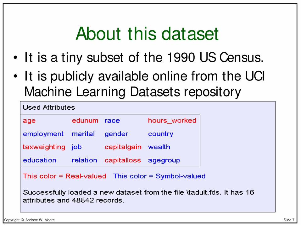
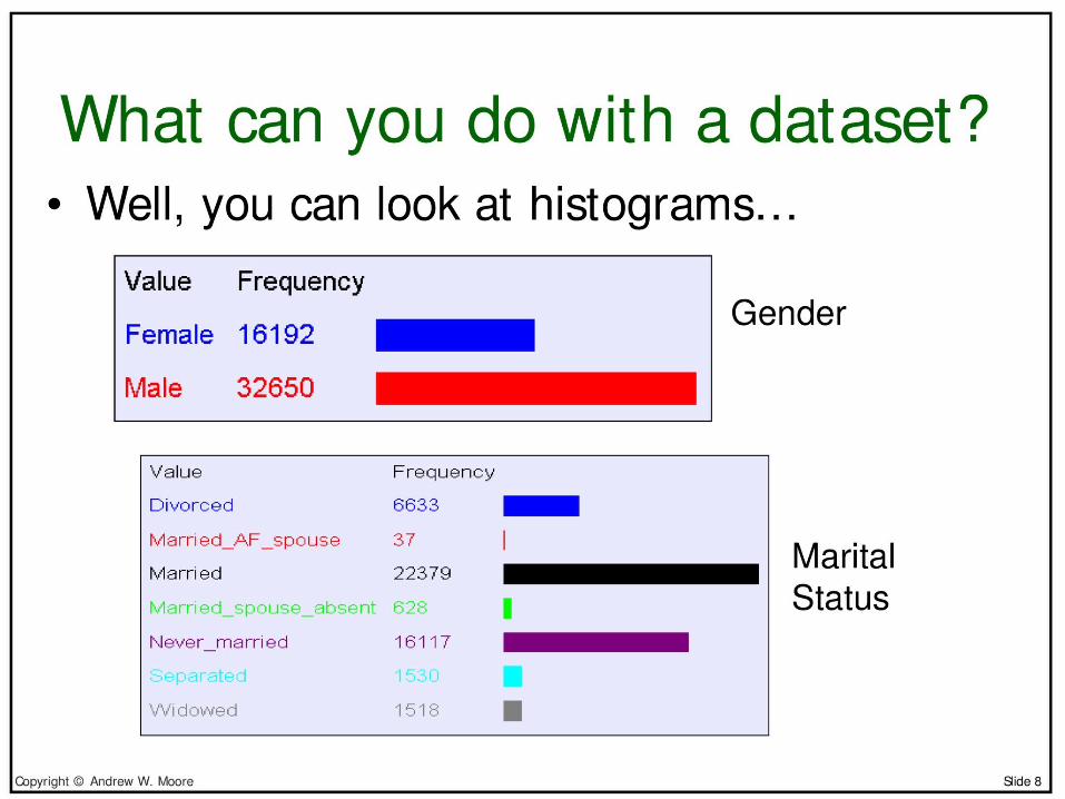
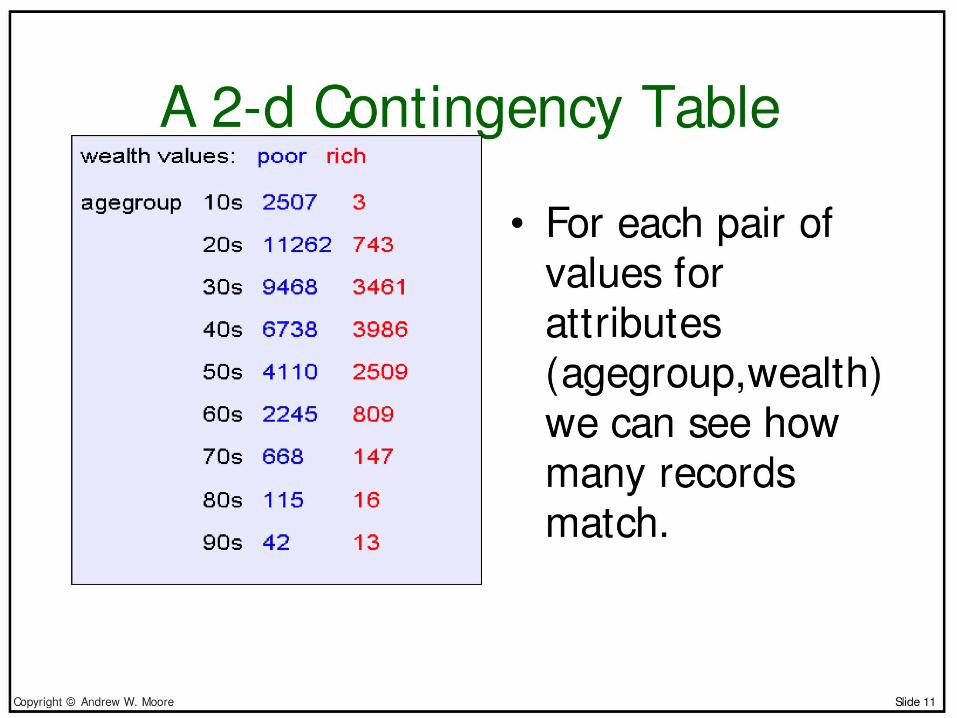
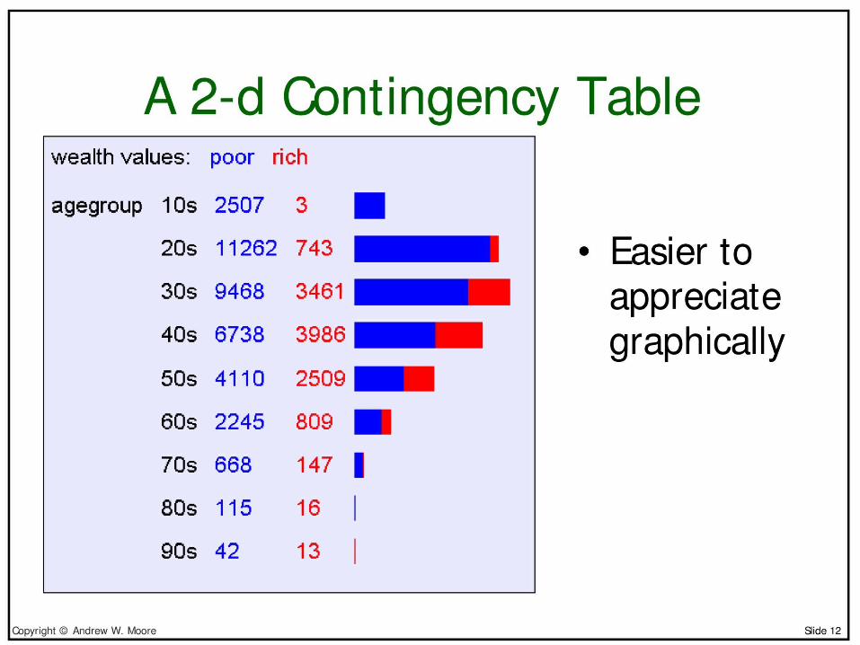
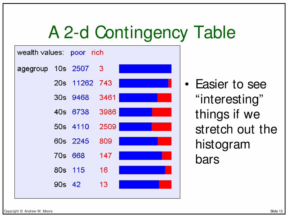
• Contingency tables– Census data set
• Information gain– Beach data set
• Learning an unpruned decision tree recursively– Gasoline usage data set
• Training error• Test error• Overfitting• Avoiding overfitting
Using this idea for classification
• We will now look at a (toy) dataset presented in Winston's Artificial Intelligence textbook
• It is often used in explaining decision trees• The variable we are trying to pick is
"got_a_sunburn" (or "is_sunburned" if you like)
• We will look at different decision trees that can be used to correctly classify this data
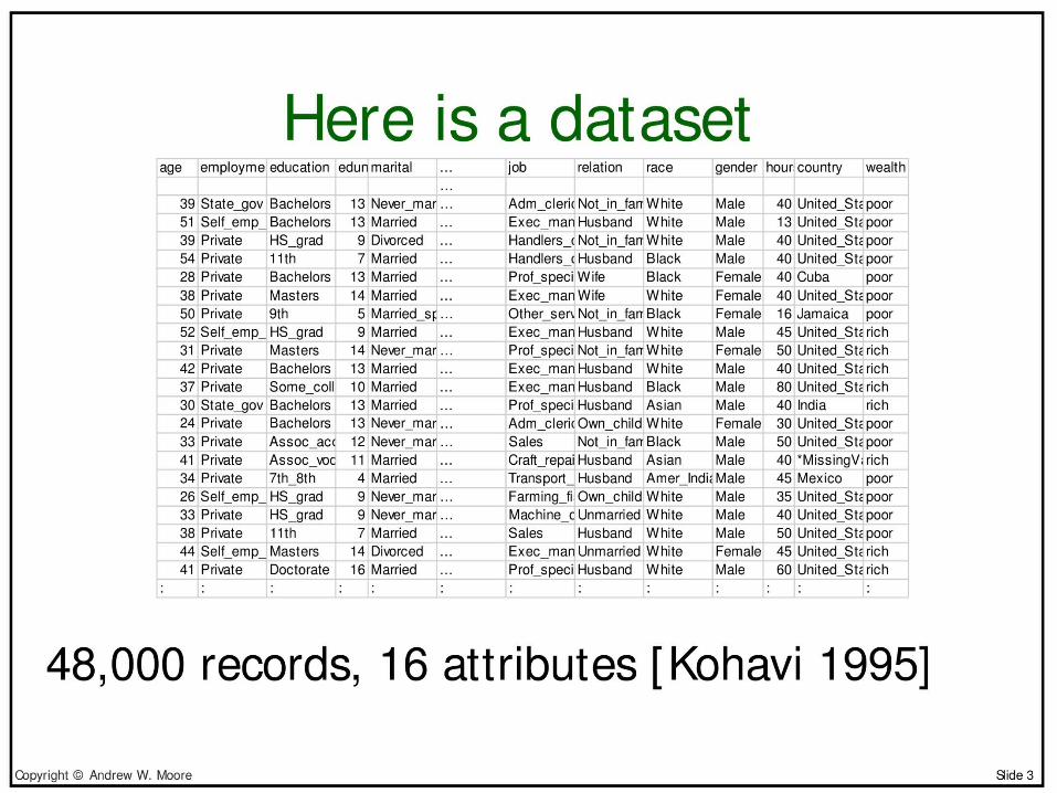
13
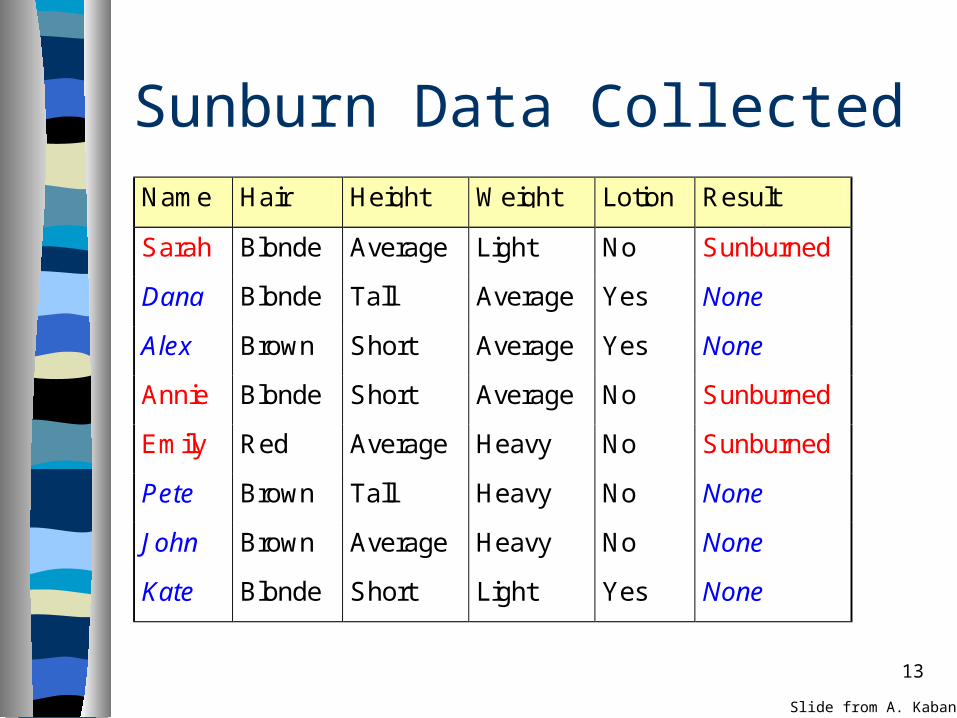
Sunburn Data CollectedName Hair Height Weight Lotion Result
Sarah Blonde Average Light No Sunburned
Dana Blonde Tall Average Yes None
Alex Brown Short Average Yes None
Annie Blonde Short Average No Sunburned
Emily Red Average Heavy No Sunburned
Pete Brown Tall Heavy No None
John Brown Average Heavy No None
Kate Blonde Short Light Yes None
Slide from A. Kaban
14
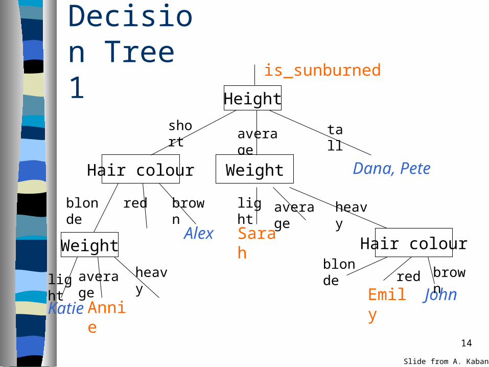
Decision Tree 1 is_sunburned
Dana, Pete
Alex Sarah
Emily JohnAnnieKatie
Height
average tallshort
Hair colour Weight
brownredblonde
Weight
light average heavy
light average heavy
Hair colourblonde
red brown
Slide from A. Kaban
15
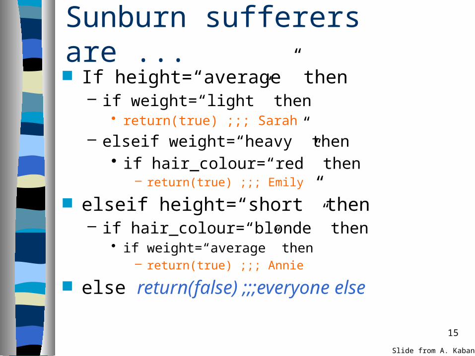
Sunburn sufferers are ... If height=“average” then
– if weight=“light” then• return(true) ;;; Sarah
– elseif weight=“heavy” then• if hair_colour=“red” then
– return(true) ;;; Emily
elseif height=“short” then– if hair_colour=“blonde” then
• if weight=“average” then– return(true) ;;; Annie
else return(false) ;;;everyone else
Slide from A. Kaban
16
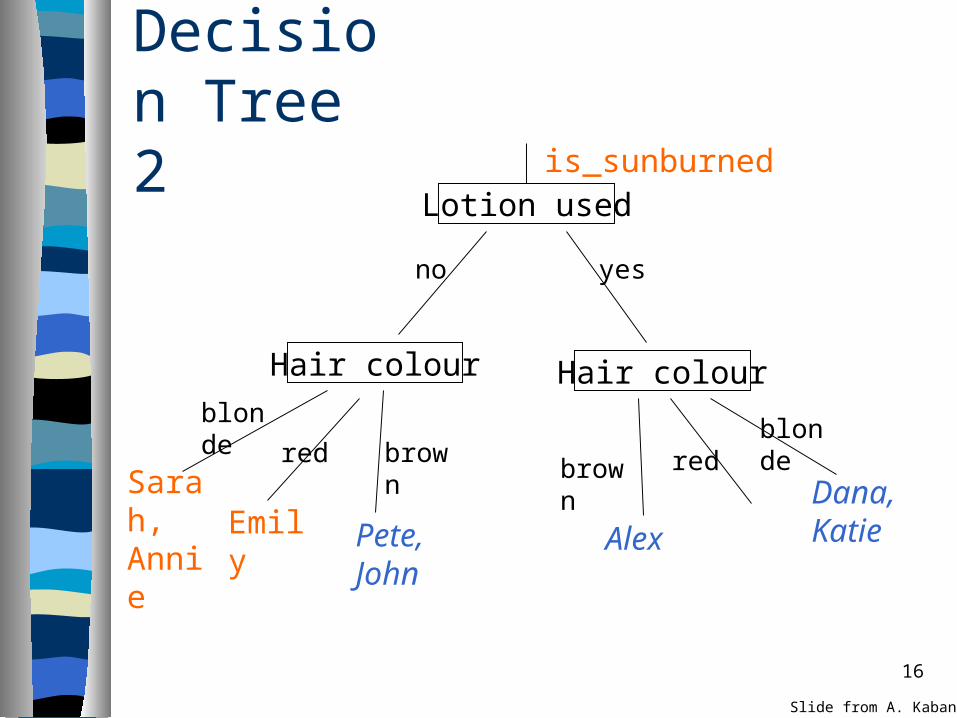
Decision Tree 2
Sarah, Annie
is_sunburned
Emily Alex
Dana, KatiePete,
John
Lotion used
Hair colour Hair colour
brownred
blonde
yesno
redbrownblonde
Slide from A. Kaban

17
Decision Tree 3
Sarah, Annie
is_sunburned
Alex, Pete, JohnEmily
Dana, Katie
Hair colour
Lotion used
blonde redbrown
no yes
Slide from A. Kaban
18
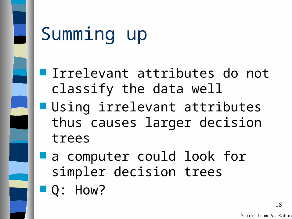
Summing up
Irrelevant attributes do not classify the data well
Using irrelevant attributes thus causes larger decision trees
a computer could look for simpler decision trees
Q: How?
Slide from A. Kaban
19
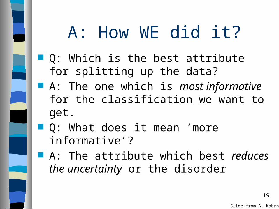
A: How WE did it? Q: Which is the best attribute for splitting up
the data? A: The one which is most informative for the
classification we want to get. Q: What does it mean ‘more informative’? A: The attribute which best reduces the
uncertainty or the disorder
Slide from A. Kaban

20
We need a quantity to measure the disorder in a set of examples
S={s1, s2, s3, …, sn} where s1=“Sarah”, s2=“Dana”, …
Then we need a quantity to measure the amount of reduction of the disorder level in the instance of knowing the value of a particular attribute
Slide from A. Kaban
21
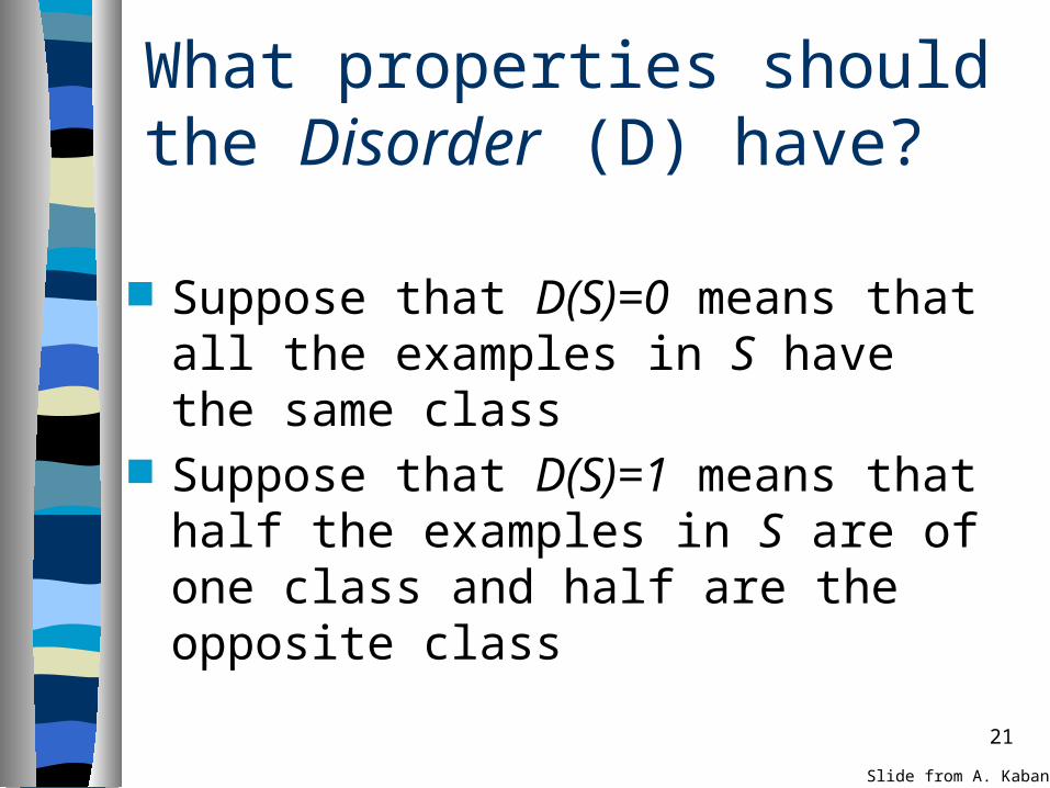
What properties should the Disorder (D) have?
Suppose that D(S)=0 means that all the examples in S have the same class
Suppose that D(S)=1 means that half the examples in S are of one class and half are the opposite class
Slide from A. Kaban

22
Examples
D({“Dana”,“Pete”}) =0 D({“Sarah”,“Annie”,“Emily” })=0 D({“Sarah”,“Emily”,“Alex”,“John” })=1 D({“Sarah”,“Emily”, “Alex” })=?
Slide from A. Kaban
23
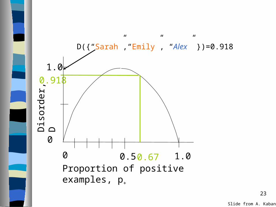
0.918
D({“Sarah”,“Emily”, “Alex” })=0.918
Proportion of positive examples, p+
0 0.5 1.0
Dis
orde
r, D
1.0
0
0.67
Slide from A. Kaban
24
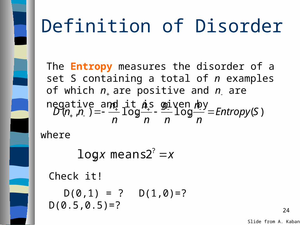
Definition of Disorder
)(loglog),( 22 SEntropy
n
n
n
n
n
n
n
nnnD
The Entropy measures the disorder of a set S containing a total of n examples of which n+ are positive and n- are negative and it is given by
xx ?2 2 means log
where
Check it!
D(0,1) = ? D(1,0)=? D(0.5,0.5)=?
Slide from A. Kaban
25
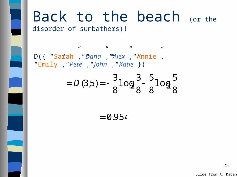
Back to the beach (or the disorder of sunbathers)!
85
log85
83
log83
)5,3( 22 D
D({ “Sarah”,“Dana”,“Alex”,“Annie”, “Emily”,“Pete”,“John”,“Katie”})
954.0
Slide from A. Kaban
26
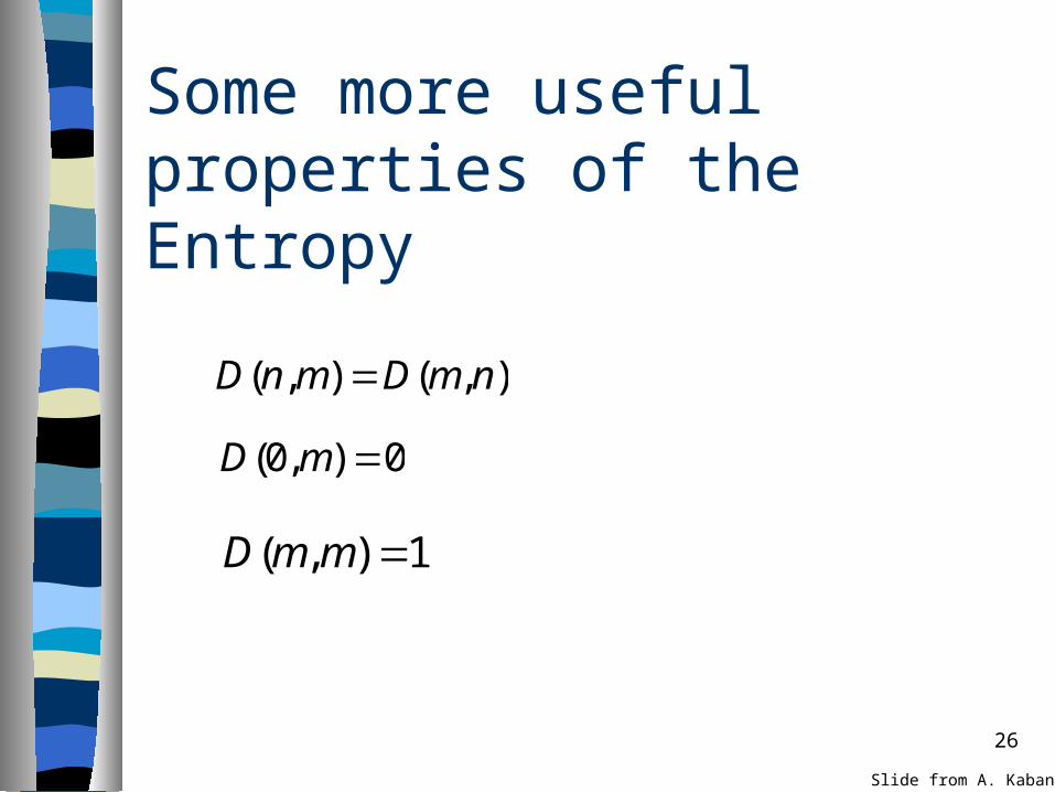
Some more useful properties of the Entropy
),(),( nmDmnD
0),0( mD
1),( mmD
Slide from A. Kaban
27
So: We can measure the disorder What’s left:
– We want to measure how much by knowing the value of a particular attribute the disorder of a set would reduce.
Slide from A. Kaban
28
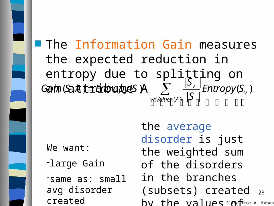
The Information Gain measures the expected reduction in entropy due to splitting on an attribute A
)(
)(||
||)(),(
AValuesvv
v SEntropyS
SSEntropyASGain
the average disorder is just the weighted sum of the disorders in the branches (subsets) created by the values of A.
We want:
-large Gain
-same as: small avg disorder created
Slide from A. Kaban

29
Back to the beach: calculate the Average
Disorder associated with Hair Colour
)( blondeblonde SD
S
S)( red
red SDS
S)( brown
brown SDS
S
Sarah AnnieDana Katie
Emily Alex Pete John
Hair colour
brownblondered
Slide from A. Kaban

30
…Calculating the Disorder of the “blondes”
5.08
4)(
S
SSD
S
S blondeblonde
blonde
The first term of the sum: D(Sblonde)=
D({ “Sarah”,“Annie”,“Dana”,“Katie”}) = D(2,2)
=1
Slide from A. Kaban

31
…Calculating the disorder of the others
The second and third terms of the sum: Sred={“Emily”}
Sbrown={ “Alex”, “Pete”, “John”}.
These are both 0 because within each set all the examples have the same class
So the avg disorder created when splitting on ‘hair colour’ is 0.5+0+0=0.5
Slide from A. Kaban
32
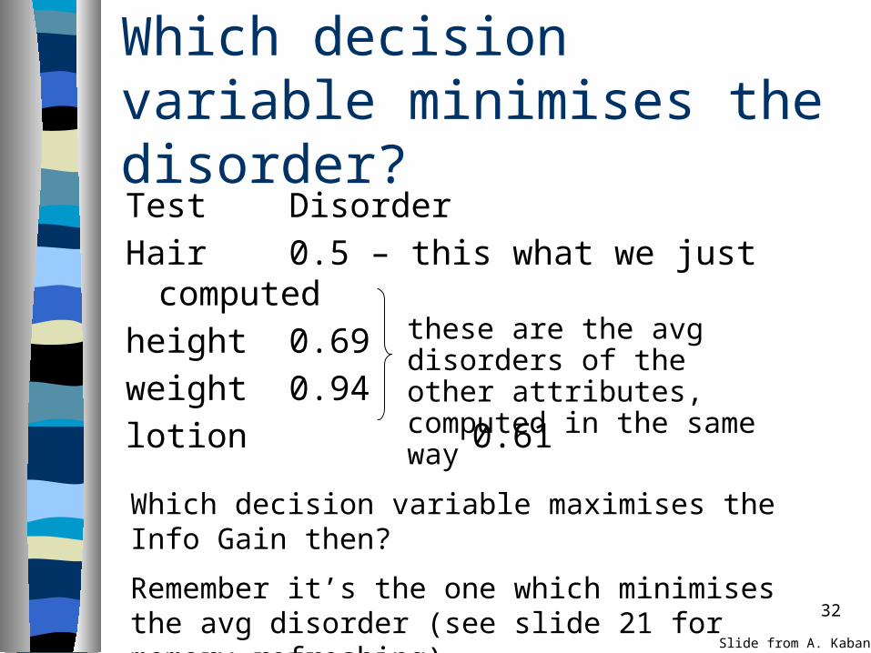
Which decision variable minimises the disorder?Test Disorder
Hair 0.5 – this what we just computed
height 0.69
weight 0.94
lotion 0.61
Which decision variable maximises the Info Gain then?
Remember it’s the one which minimises the avg disorder (see slide 21 for memory refreshing).
these are the avg disorders of the other attributes, computed in the same way
Slide from A. Kaban
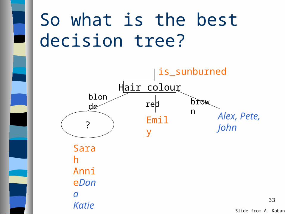
33
So what is the best decision tree?
?
is_sunburned
Alex, Pete, John
Emily
Sarah AnnieDana Katie
Hair colour
brownblonde
red
Slide from A. Kaban
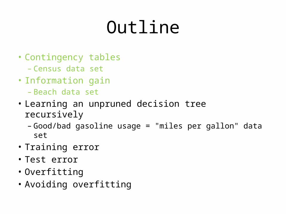
Outline
• Contingency tables– Census data set
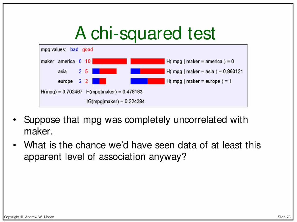
• Information gain– Beach data set
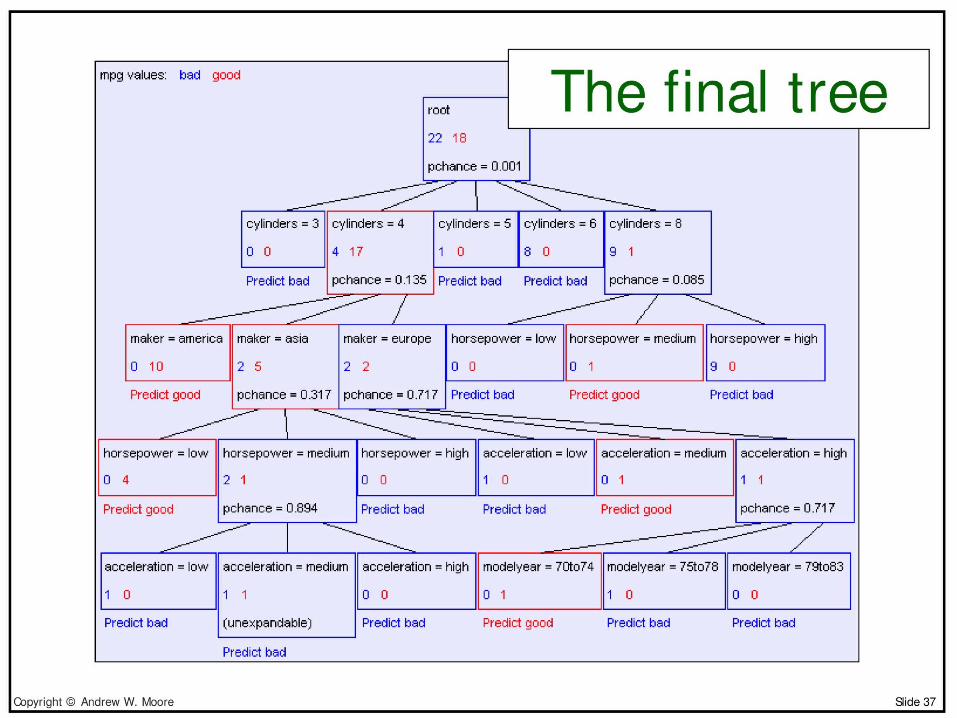
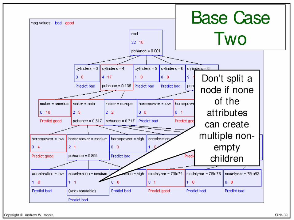
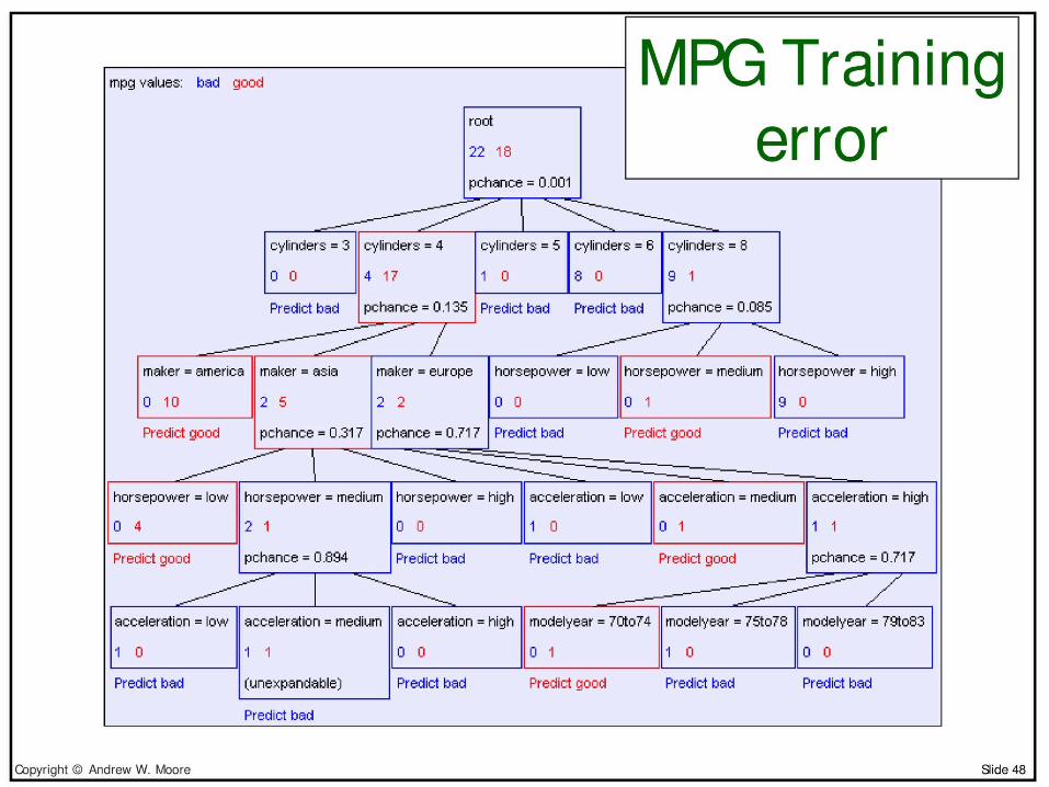
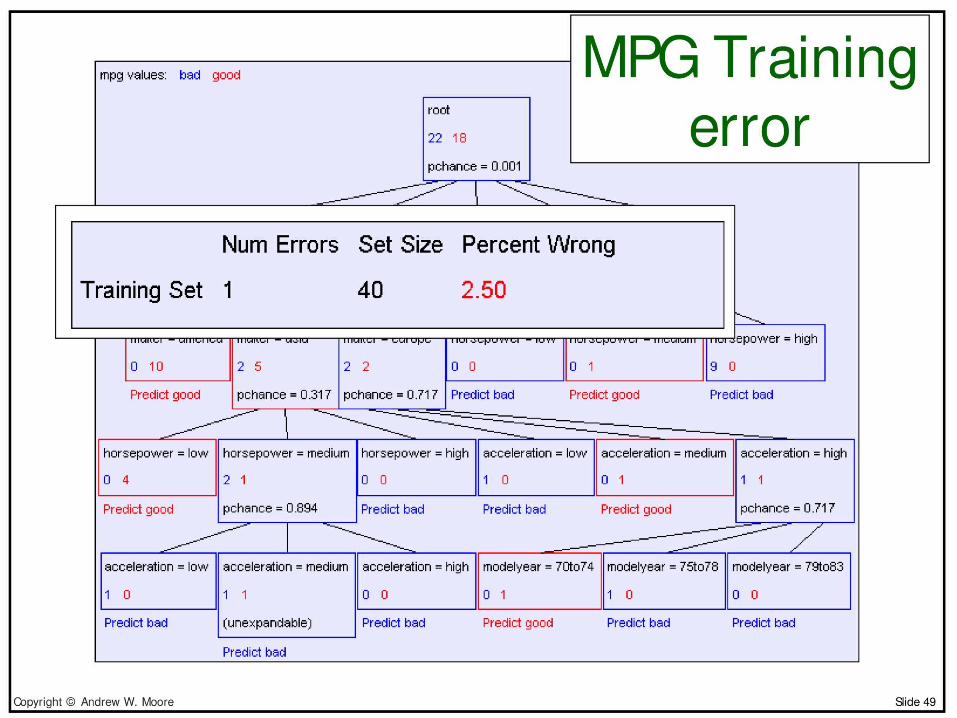
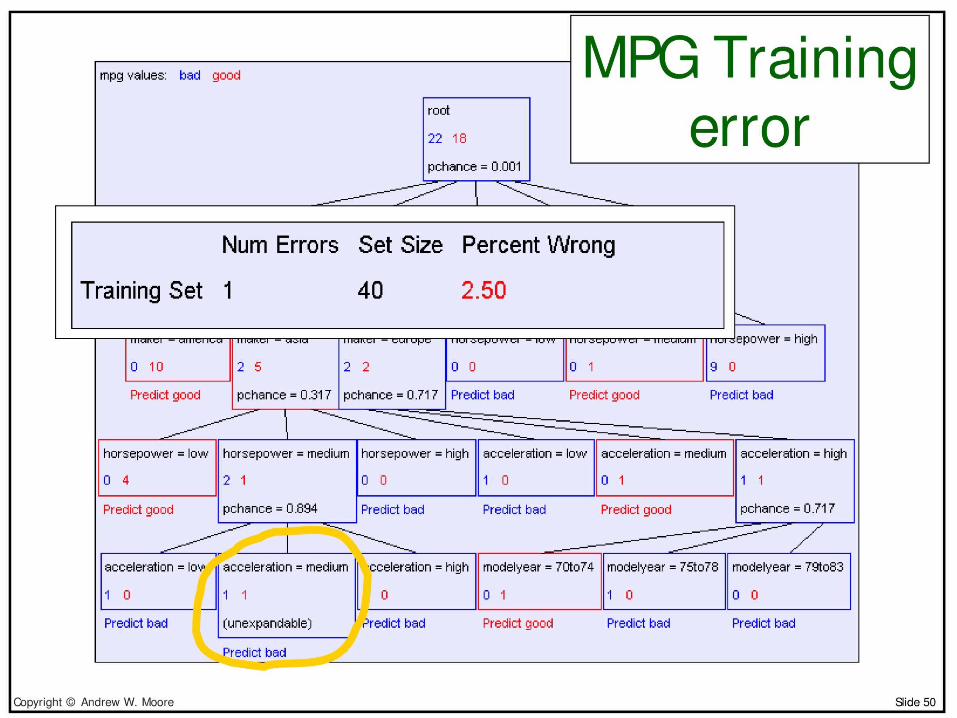
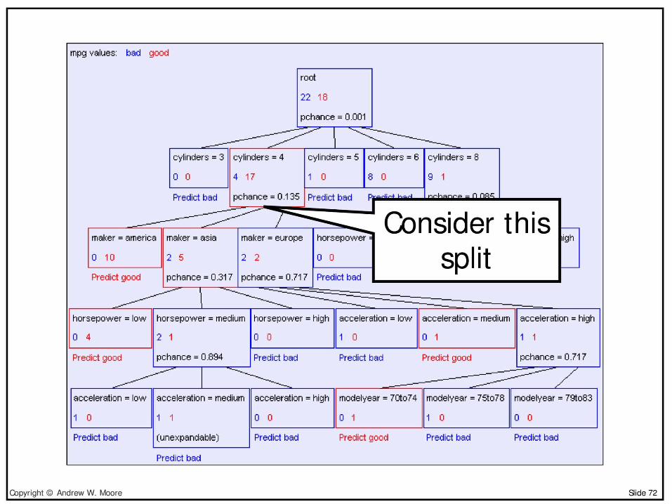
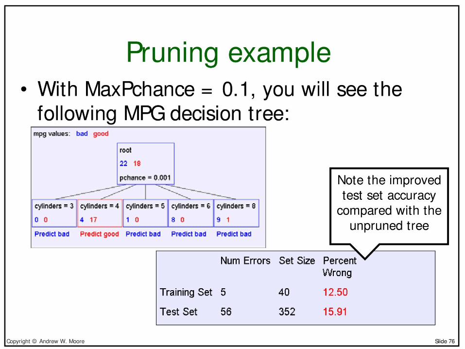
• Learning an unpruned decision tree recursively– Good/bad gasoline usage = "miles per gallon" data set
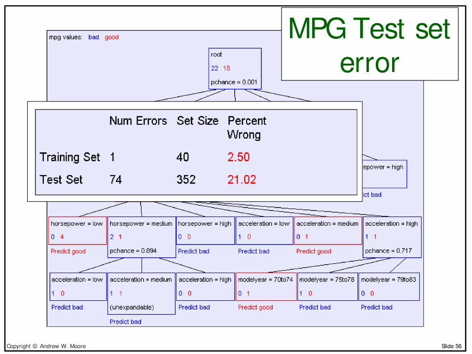
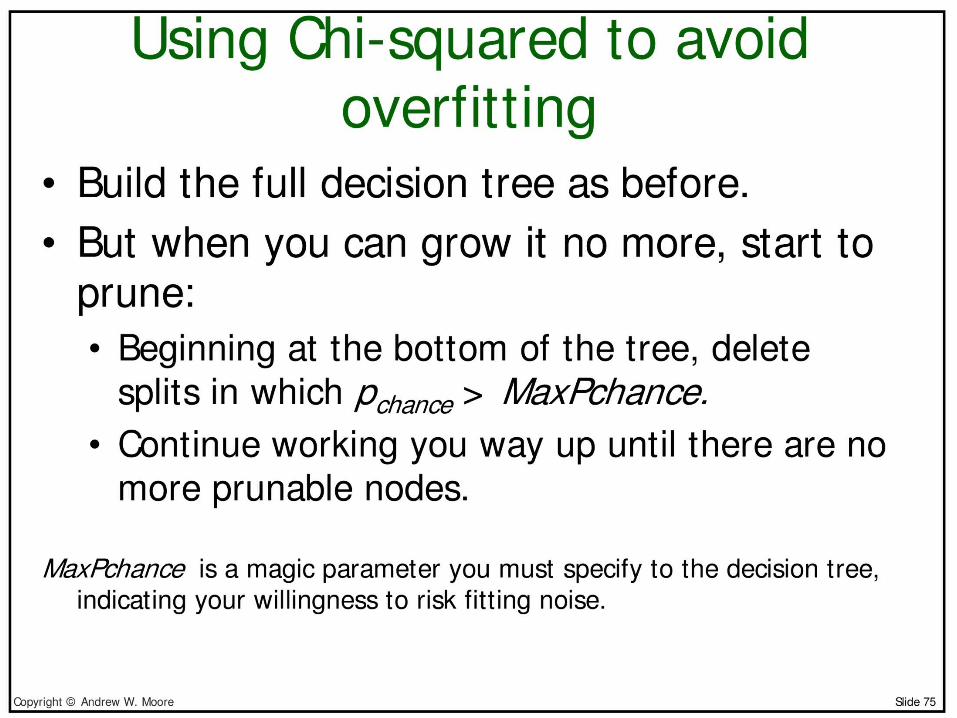
• Training error• Test error• Overfitting• Avoiding overfitting


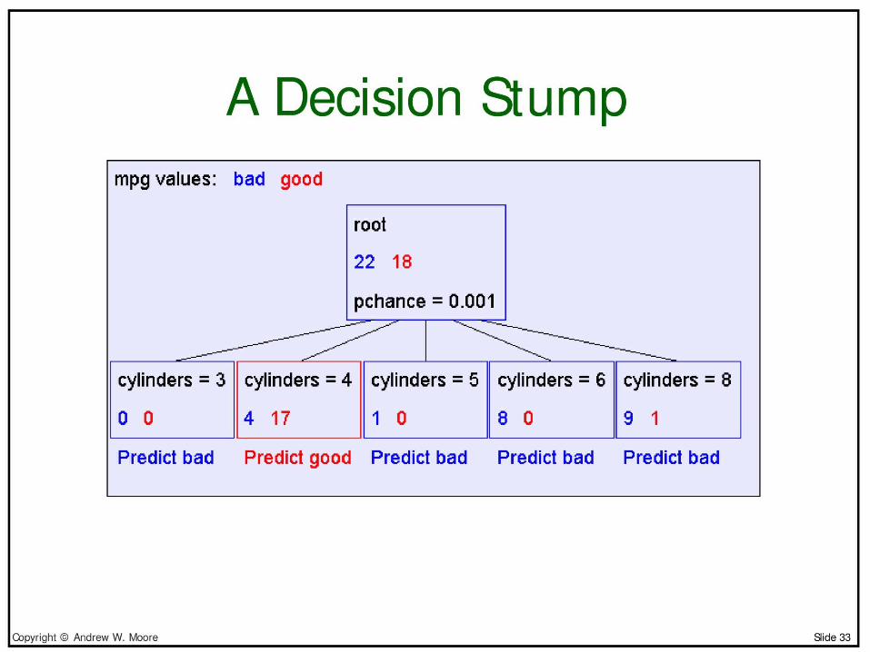
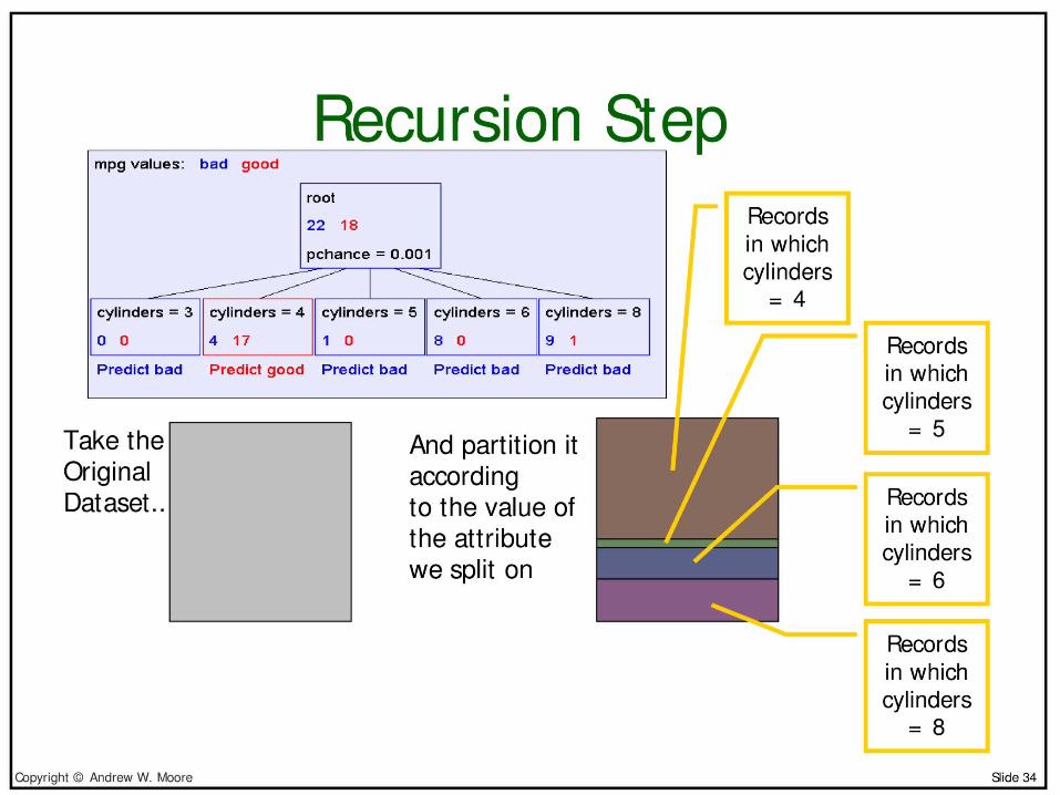
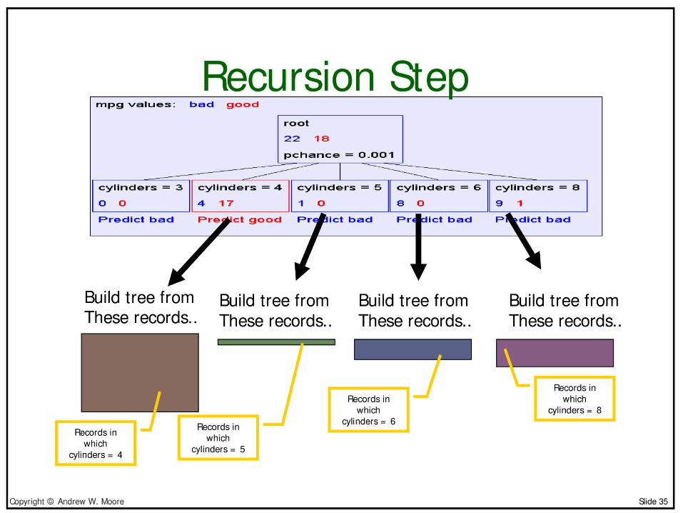
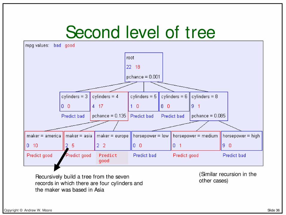
Predict good


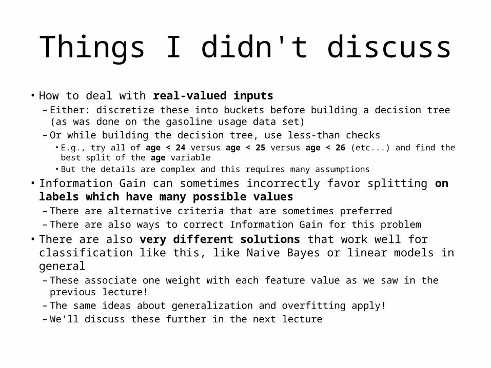
Things I didn't discuss• How to deal with real-valued inputs
– Either: discretize these into buckets before building a decision tree (as was done on the gasoline usage data set)
– Or while building the decision tree, use less-than checks• E.g., try all of age < 24 versus age < 25 versus age < 26 (etc...) and find the best split of the age
variable• But the details are complex and this requires many assumptions
• Information Gain can sometimes incorrectly favor splitting on labels which have many possible values– There are alternative criteria that are sometimes preferred– There are also ways to correct Information Gain for this problem
• There are also very different solutions that work well for classification like this, like Naive Bayes or linear models in general– These associate one weight with each feature value as we saw in the previous lecture!– The same ideas about generalization and overfitting apply!– We'll discuss these further in the next lecture

65
• Slide sources– See Ata Kaban's machine learning class
particularly for the intuitive discussion of the Winston sunburn problem and Information Gain
– See Andrew W. Moore's website for a longer presentation of his slides on decision trees, and slides on many other machine learning topics:
http://www.autonlab.org/tutorials
66
• Thank you for your attention!


