1

Infrastructure Development and Poverty Reduction:

Evidence from Cambodia’s Border Provinces

Phim Runsinarith

Graduate School of International Studies

Nagoya University

2

1. Introduction

At the end of the 20th century, governments around the world agreed on a set of

common goals for developing countries, known as the Millennium Development Goals.

These goals pave the way forward to cut world poverty by half by 2015. Cambodia has

also made efforts to achieve the goal. Among other things, infrastructure has been seen as

one important factor for poverty reduction and its potential effects on improving

livelihood are raised in Cambodia Millennium Development Goals (CMDGs). Investing

in pro-poor rural infrastructure such as small-scale irrigation facilities, all weather roads,

rural electrification and physical market infrastructure will stimulate production, enhance

productivity and facilitate trade and labour mobility (RGC 2003).

In Cambodia, the poor barely have any access to basic social services and facilities. A

WB report on poverty profile in Cambodia in 2004 states that the poorest quintile have to

travel 7 kilometers to reach a communal health center, while the richest quintile do not

have to travel that far. People in the poorest quintile, on average, live twice as far from the

nearest road as those in the richest quintile. About 60 percent of the richest quintile have

access to publicly provided electric lighting, while less than 15 percent in the poorest

quintile receive the same service. The same report also indicates that only 2 percent of

people in the poorest consumption quintile have access to piped water compared to 36

percent in the richest consumption quintile. Similarly, access to sanitation facilities by the

poor is very limited or non-existent. More than 90 percent of the people in the poorest

quintile have no access to or do not use toilet facilities.

The significance of expected contribution of infrastructure to economic development

and poverty reduction has been widely recognized and infrastructure investment has been

put on top priority list on the government’s development agenda. The RGC’s Rectangular

Strategy fully acknowledges that among other things, continued rehabilitation and

construction of physical infrastructure – which include continued restoration and

construction of transport infrastructure, management of water resources and irrigation,

development of energy and power grids, and development of Information and

Communication Technology – are crucial for promoting sustainable development and

poverty reduction (RGC 2004).

Although there are plentiful assumptions regarding the potential effects of

infrastructure development on poverty reduction, quantitative studies to measure those

effects remain scarce. This paper attempts to fill the gap by addressing two questions: (1)

Who are the poor? and (2) How could infrastructure help reduce poverty?

To answer the first question, poverty incidence, poverty gap, poverty severity by

location, household characteristics, sources of income and access to infrastructure, will

3

be computed based on an updated poverty line and poverty formula proposed by Foster,

Greener and Thorbecke. Gini coefficients will also be computed to examine inequality

between the worse-off and the better-off groups. Two different regression techniques:

Ordinary Least Square with robust option and quantile regression will be employed to

investigate the impact of infrastructure on per capita consumption. Household survey

data collected in 2006 in two border provinces of Cambodia will be utilized for analysis.

It is worth noting that those provinces which are on the so-called economic corridors of

the Greater Mekong Sub-region (GMS) are where infrastructure is most directly affected

by increased regional integration.

The next section develops a basic framework for analysis. It will discuss how

infrastructure which includes cell phone, irrigation, electricity and road would impact on

household welfare. Section 3 elaborates the methodology of how data are collected and

how poverty line, poverty indices and Gini coefficient are constructed. Section 4

examines poverty profile of households in the border province by decomposing poverty

incidence, poverty gap, poverty severity and inequality coefficient by location, household

characteristics, sources of income, and access to infrastructure. Section 5 provides some

notes on regression techniques used in the paper and discusses the effects of infrastructure

on per capita consumption and poverty reduction. Section 6 is the conclusion and policy

recommendation section.

2. A Framework

This paper follows neo-classical growth model approach to scrutinize the effect of

infrastructure on poverty reduction. The neoclassical growth model effectively highlights

an important correlation between economic growth and poverty reduction. This model

theorizes that economic growth is contingent upon the accumulation of capital, both

human and physical, and technological progress. Human capital refers to the increase in

labor productivity due to levels of education, skills and experience, and the health of the

people. Physical capital represents the tools used in production. Lastly, technological

progress has a two-fold meaning: it is the ability of larger quantities of output to be

produced with the same quantities of capital and labor. Equivalently, technological

progress represents the key ingredient in developing new, better and a larger variety of

products for the public to consume. Based on this neo-classical theory, physical capital

infrastructure is assumed to exert positive impact on economic growth as through

increased labor productivity.

Existing literatures have demonstrated the existence of a positive relationship

between infrastructure investment and economic growth as well as the existence of a

4

strong connection between economic growth and poverty reduction. Some earlier works

on infrastructure investment found that public expenditure on infrastructure yields a very

positive impact on economic growth (Easterly and Rebelo, 1993; Canning, 1998;

Calderon and Servon 2004; Phim 2004). This suggests that it is worth investing more on

infrastructure if achieving economic growth is the goal. Other literatures on economic

growth and poverty have also found a positive relationship between economic growth and

poverty reduction and concluded that growth is good for the poor (Dollar and Kraay

2000) or that economic growth and poverty reduction clearly go largely hand in hand

(Rodrik 2000).

The analytical framework in this paper is simply adopted from the neo-classical

model theory above with an attempt to show how infrastructure would impact on

economic well-being through improved productivity.

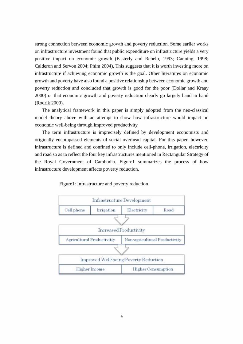
The term infrastructure is imprecisely defined by development economists and

originally encompassed elements of social overhead capital. For this paper, however,

infrastructure is defined and confined to only include cell-phone, irrigation, electricity

and road so as to reflect the four key infrastructures mentioned in Rectangular Strategy of

the Royal Government of Cambodia. Figure1 summarizes the process of how

infrastructure development affects poverty reduction.

Figure1: Infrastructure and poverty reduction

5

Cell phones can raise welfare of the poor. Grameen Village Phone of Bangladesh

provides a good case of how phones may increase the productivity and welfare of

villagers in developing countries. The Village Phone program yields significant positive

social and economic impacts, including relatively large consumer surplus and

immeasurable quality of life benefits (Don Richardson, Ricardo Ramirez, Moinul Haq,

2000). Besides reducing risks of remittance transfer, phones could help villagers get

accurate information about market prices, market trends and exchange rates, which will

consequently lead to reduction in unnecessary costs and increase in profitability.

Irrigation is expected to be growth-enhancing and poverty reducing. There is

evidence showing that irrigation significantly contributes to farm productivity and wages,

reducing poverty. Research in India, Philippines, Thailand, and Vietnam suggests that

poverty is substantially lower in irrigated areas compared with unirrigated areas

(Bhattarai et al, 2002). In an agrarian economy where a vast majority of population still

depends on agriculture for livelihood, water is dispensable for crop cultivation and

irrigation will play an important role to improve farm productivity.

Electricity is proved to have big favorable impacts on the livelihood of rural people.

Not only it can be used for lighting and household purposes but it can also be used for

mechanization of agriculture which allows for greater productivity at reduced cost. An

evaluation of Word Bank-assisted rural electrification projects in Asia indicates that rural

electrification in Bangladesh and India raises the use of irrigation, thereby significantly

reducing poverty incidence (Songco 2002). It is expected that through improved

productivity in farm and non-farm activities, electricity will also bring a positive impact

to poverty reduction in both of the sample border provinces.

Like previous infrastructure mentioned above, road development is a means for

poverty reduction. A good road network system supported by an appropriate level of

transport services can lower costs and prices. This enhances economic opportunities for

the poor and helps reduce poverty. A road investment could result in an increase in

agricultural productivity, non-farm employment and productivity, directly raising the

wages and employment of the poor and, hence, their economic welfare. In addition,

higher productivity and expanded employment would lead to higher economic growth,

affecting the supply and prices of goods and, thus, the well-being of the poor (Ifzal Ali

and Ernesto Pernia 2003).

Overall, development in such infrastructure as phones, irrigation, electricity and roads

is expected to create employment and help increase productivity in farm and non-farm

sectors which eventually brings benefits to remote households who tend to be poor (this

will be discussed in greater detail in the next section).

6

3. Data and Poverty Measurement

3.1 Data

In this paper, a set of survey data of National Institute of Statistics (NIS) from two

provinces, Banteay Meanchey and Svay Rieng in 2006 is used to measure and explain the

poverty impact of infrastructure. The data set consists of 600 households in Banteay

Meanchey and 599 households in Svay Rieng. The dependent variable is the natural

logarithm of per capita household expenditure, lny. The total household expenditure is

grouped into three categories (i) Food items, (ii) Non-food items that are consumed more

frequently/regularly and (iii) Other non-food items which are not so frequently consumed.

Per capita consumption expenditure is calculated by dividing the total household

expenditure by the household size.

3.2 Poverty Measurement

Poverty Line

Three poverty lines for three different areas: Phnom Penh, other urban areas and rural

areas, were constructed in Cambodia. In this paper, poverty lines of other urban and rural

areas in 2004 are updated with the rates of inflation occurred from 2005 to 2006.

Specifically, because the poverty line was 1,952 riel in other urban and 1,753 riel in rural

areas are 1,952 riel and according to the figures produced by CDRI, inflation rate were 16

percent in 2005, the poverty updated line is 2,264 riel for other urban and 2,033 riel for

rural areas. If one’s consumption expenditure is below 2,264 riel per day, he is classified

as a poor in other urban areas and if below 2,033 riel, a poor in the rural areas.

Poverty Indices

Poverty headcount, poverty gap, and poverty severity in Table1, are constructed

following the formula proposed by Foster, Greener and Thorbecke (1984).

q

i

i

z

yz

NP

1

1

(1)

where

N = total population

yi = welfare indicator, e.g., consumption per cap

z = poverty line

q= number of poor in the population

yi , …, yq < z < yq+1 … yn

7

The Foster, Greener and Thorbecke (FGT) measures are defined for ≥ 0, with as

a measure of the sensitivity of the index to poverty. If = 0, equation (1) becomes the

headcount index P0. If = 1, it becomes the poverty gap index P1 and if = 2, the

poverty severity index P2.

The Headcount Index denoted as P0 is the proportion of the population for whom, per

consumption is below the poverty line. But this headcount index has a disadvantage

because it assumes all the poor are in the same situation. The poverty gap index P1 gives a

better idea of how deep poverty is as it reflects the average shortfall of the poor. Despite

this virtue the poverty gap index does not capture differences in the severity of poverty

amongst the poor and ignore ―inequality among the poor‖. The poverty severity index or

the squared poverty gap index P2 takes inequality among the poor into account by having

weights given to each observation and by putting more weight on those that fall well

below the poverty line.

Inequality

Poverty measures focus on the situation of persons or households at the bottom of the

consumption distribution. Inequality is a broader concept than poverty in that it is defined

over the entire population. A measure of inequality attempts to capture the deviation of a

given distribution of consumption from the ideal distribution, called perfect equality.

In this paper, Gini coefficient which is the most commonly used measure for

inequality is also computed along with the poverty indices above. The Gini coefficient is

calculated with the following formula:

N

i

i

ii

yN

fyCovGini

1

1

),(2 (3)

where

yi is the expenditure of household i

fi is the rank of household i in the distribution

(f varies between 0 for poorest and 1 for richest)

4. Poverty Profile of the Border Provinces:

Location: Among the two provinces, Banteay Meanchey is found to have higher

poverty incidence (P0) than Svay Rieng. Across all provinces, both border rural and rural

non-border households which make up 70 percent of the total surveyed population,

8

respectively have 44 percent and 47 percent of population living below poverty line while

only 25 to 29 percent of urban households are found to be poor. This finding indicates that

poverty is largely a rural phenomenon. The poverty gap P(1) poverty severity P(2) are

lower in Svay Rieng than in Banteay Meanchey meaning that the poor are less poor and

the gap among the poor is smaller in the former province. However it seems that overall

inequality is higher in areas where poverty rate is lower. Table1 shows that Gini

coefficient is relatively smaller in Svay Rieng and rural stratum implying that the gap

between the rich and the poor is relatively narrower.

Household Characteristics: Poverty rate and inequality are a bit higher with

households headed by female. This finding conforms well to previous studies which

showed that female-headed households are usually poorer than male-headed households.

As far as age is concerned, poverty incidence increases when the age of household head

increase and is the highest among 50-60 year-old group. The inequality, however, is high

among 30-40 and 40-50 year-old groups. When it comes to education, poverty rate

decreases as the education level of household heads increase. About 68 percent of heads,

however, never finished primary education and the poverty rate, poverty gap and poverty

severity is highest among this group.

Sources of Income: Of households in both provinces, 14 percent of them are cross

border traders and 33 percent are cross-border workers. Poverty incidence, poverty gap,

and poverty severity are found to be highest among the later group, indicating that the

number of the poor is higher, the poor are relatively poorer, and the inequality among the

poor is larger within cross-border workers as compared to other groups. Nevertheless, the

overall disparity between the rich and poor is highest among the trader group. Breaking

down by sources of income, it is found that 51 percent of households earn money from

cultivation of cereal crops, 16 percent from manual labor, and 17 percent from own

enterprises. Poverty rate is higher than the average for many groups. Among those who

rely on cultivation of cereal crops and manual labor, the respective poverty rate is 43

percent and 56 percent. The poverty gap and poverty severity index suggest that the poor

in manual labor group is relatively poorer and the inequality is relatively higher than any

other groups. Consistently the Gini coefficient is highest in the groups with lower poverty

rate.

Access to Infrastructure

Cell phone: During the surveyed period only 17 percent of households in the sample

are found to have cell phone. Among the households that have this communication

equipment only 11 percent of them lives below the poverty line. The poverty gap and

9

poverty severity are also found lower among this group. However the overall gap

between the rich and the poor is relatively larger compared to the group having no phone.

Electricity: Access to electricity is very limited in the border provinces. Only 15

percent of households are found to have access to city power during the surveyed period.

As shown in Table1 many households use kerosene (42 percent) or battery (40 percent)

for lighting. The poverty incidence, poverty gap, and poverty severity are relatively

higher among households that use kerosene. The gap between the better-off and the

worse-off, however, is relatively larger among households that use city power.

Irrigation: The majority of population has no access to irrigation system. Only some

28 percent of household were able to access to irrigation system. Poverty rate and Gini

coefficient are found to be highest within the households who did not have access to

irrigation system. However no noticeable differences in poverty gap and poverty severity

are detected between these two groups. Investment in irrigation system would greatly

benefit the poor as most of them rely on cultivation of cereals for livelihood.

School: Of the total households in the sample, 75 percent of them live far from a

primary school. As can be seen, the poverty rate is higher when households locate farther

from the school – ranging from 35 percent for the group that lives within 200 meters to 42

percent with group that lives between 1km and 5 km far from school. The poverty gap and

poverty severity are higher within groups living far away from school. Being near school

seems not only to provide opportunity for the children from all socio-economic status

groups to attend class but also give them more time to directly or indirectly help

household business. As a result, households near school tend to have relatively better

economic status.

Health Center: Almost all of households live farther than 200 meters from a health

center. Health center is relatively scarce compared to primary school. Like in the case of

primary school, households who live farther away from a health center tend to be poorer.

The poverty rate varies from 24 percent with group of households within 200 meter

distance to 45 percent with group of households beyond 5 km away from the center.

Again the Gini coefficient is larger within the lower poverty rate groups.

Road: Some 69 percent of the surveyed households live farther than 1km from a

main road and 37 percent of them live below the poverty line. Inequality is found to be

high with groups of lower rate of poverty. Being near the main road enhances chance for

households to engage with business activities. Being near the main road also facilitates

households to access to social services including electricity, irrigation, school, and health

center mentioned above. Therefore, a relatively small percentage of households who live

near the main road are found to be poor.

10

11

Regression Analysis

Model Specification

A model used for regression analysis is developed from per capita consumption

model which has been used in many poverty studies. The basic consumption model

theorizes per capita consumption as a function of a set of household characteristic

variables including household size, assets, education, and sanitation. However, it is

arguable that development level of an area could play significant role in poverty

determinants. Further, variables, which represent for development level, should also be

included into the basic model to reflect the effect of development on consumption.

However, as discussed in Section 2, the neo-classical framework posits that economic

growth can be achieved by increase in capital, either human or physical, and

technological progress. Since infrastructure would increase capital productivity, it is also

safe to assume that infrastructure would increase economic growth or per capita income.

Here, per capita consumption is used as a proxy of per capita income. Incorporating a set

of development variables and a set of infrastructure variables into the basic per capita

consumption equation, a model to detect the impact of infrastructure can be specified as

follow:

(3)

where

is a per capita consumption of household i

is a vector of household characteristic variables.

is a vector of development level variables

is a vector of infrastructure variables and

It is worth noting that as development level and infrastructure variables can be

correlated; there is a need to enter these two groups of variables into the estimation

equation separately. Estimation (2), (3) and (4) in both OLS and quantile regression are

created in order to address such multi-collinearity issue. It should also be noted that the

coefficients in these semi-log equations have the interpretation of percentage changes, not

changes in levels. This is because the dependent variable is the log per capita expenditure

not the per capita expenditure itself, and the changes in logs equal the percentage change

in levels.

12

Description of Explanatory Variables

The explanatory variables include household characteristics, the development level

of the area, and the infrastructure variables. As mentioned earlier, the household

characteristics include household size, education of household head, sanitation, land size,

land title and hand-tractor. The basic concepts of these variables and their relationships to

the welfare are briefly explained below.

HHS is the household size or the number of household members. In general, the

larger the household size the smaller the per capita consumption expenditure. Thus the

sign of the household size coefficient is expected to be negative.

Education is the educational level of the household head. In the current survey,

people were asked the highest educational level that he/she has successfully completed

and codes were used to represent their grade level. Here, the variable is classified into 6

categories: 1 no education, 2 primary, 3 lower secondary, 4 upper secondary, 5 college

graduate, 6 post graduate. The sign of the coefficient of Education would be positive, as

on average, higher levels of education are associated with higher income and hence

higher per capita expenditure.

Sanitation is a dummy variable indicating whether or not a household have a toilet. It

takes value one if household possesses a toilet and zero otherwise. As a large proportion

of diseases are caused by limited access to sanitation, the poor are particularly susceptible

to health-related outcomes arising from poor sanitation (Murshid and Phim 2005). The

sign of the coefficient of Sanitation would be positive because household with knowledge

of sanitation would less frequently suffer from ill-health and therefore could more

productively engage with income generating activities which would in turn result in

relatively higher per capita expenditure.

Land is the area of land owned by households. Land is considered to be the most

valuable asset for farmers and the size of land owned by households is often used as

household welfare indicator. The better off households generally possess larger

agricultural land and hence they are able to produce and consume more than the worse off

ones. Per capita consumption expenditure would then be expected to be positively

associated with this independent variable.

Title is a dummy variable showing if the land owned by household has any certified

document. Households which lack secure land rights are vulnerable to land grabbing,

encroachment, and other types of conflicts (CDRI 2008). This in turn reduces investment

incentives, even when capital resources are available. Those households are also unable

or otherwise reluctant to assume the risks associated with variable soil and climate

conditions, especially drought and floods. Hence, household that owns land with secure

13

title is expected to use that land more productively and would be able to generate higher

income and afford higher per capita expenditure.

Tractor is a variable of household that has productive asset. Evidence from CDRI’s

Moving Out of Poverty study conducted in nine villages showed that not only that tractor

or hand-tractor can be used as farming tools but they can also be used as taxi to transport

people to make extra earning.

Urban is a dummy variable denoting a development level of an area. It takes value

one if a household live in urban area and zero if in rural. Urban dummy variable is

expected to have a positive sign because urban is expected to have more economic

activities which can provide employment to urban residents.

Border is an integration intensity variable with regional economy. This border

dummy is set to one if household resides near border and zero otherwise. The economic

activities are observed to be more intensified in the border areas compared to others.

Many migrants come to get benefits that border can offer which include cross border

trade and cross border work (Phim et al 2007). Household that resides in border areas are

expected to economically benefit from cross border interaction and afford higher

expenditure.

Phone is dummy variable indicating whether or not a household has a technology to

communicate with others. It is widely accepted that information has economic value

because it allows households to make choices that yield higher expected payoffs or

expected utility than they would obtain from choices made in the absence of information.

Hence households with information equipment are expected to have higher welfare than

those without it.

Irrigation is a dummy variable which represents whether or not households have

access to irrigation system. Irrigation has been seen as a way to reduce poverty of rural

households. Anders Engvall and Ari Kokko (2007) suggest that irrigation along with land

improvement provides additional improvements in human development outcomes. As

irrigation is expected to improve the livelihood of households who has access to it, the

sign of Irrigation would be positive.

Electricity is a dummy variable indicating whether or not households have access to

electricity. The importance of energy to development is well documented and there is

empirical basis to the relationship between access to modern technology and human

development (UN Millennium Project 2005). Electricity is expected to have positive sign

as households who can access to electricity may be able to expand opportunities for other

businesses and improve household welfare.

Mroad is a dummy variable that represents the proximity to the main road. To

14

construct the road dummy, the distance of 200 meters away from the main road is used as

the cutting point. Mroad is set to 0 if households locate farther than 200 meters from the

main road and set to zero otherwise. Households located near the main road are expected

to receive greater economic benefits and so its coefficient sign would be positive.

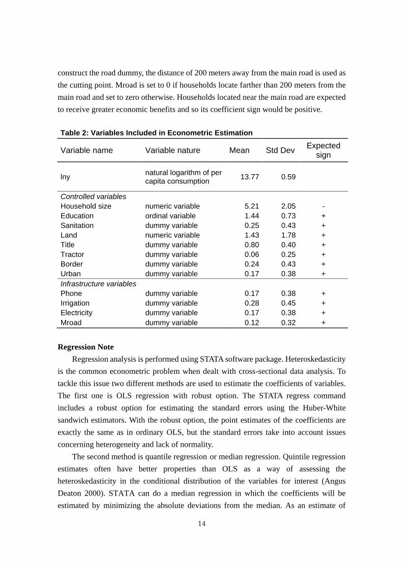
Table 2: Variables Included in Econometric Estimation

Variable name Variable nature Mean Std Dev Expected

sign

lny natural logarithm of per capita consumption

13.77 0.59

Controlled variables

Household size numeric variable 5.21 2.05 -

Education ordinal variable 1.44 0.73 +

Sanitation dummy variable 0.25 0.43 +

Land numeric variable 1.43 1.78 +

Title dummy variable 0.80 0.40 +

Tractor dummy variable 0.06 0.25 +

Border dummy variable 0.24 0.43 +

Urban dummy variable 0.17 0.38 +

Infrastructure variables

Phone dummy variable 0.17 0.38 +

Irrigation dummy variable 0.28 0.45 +

Electricity dummy variable 0.17 0.38 +

Mroad dummy variable 0.12 0.32 +

Regression Note

Regression analysis is performed using STATA software package. Heteroskedasticity

is the common econometric problem when dealt with cross-sectional data analysis. To

tackle this issue two different methods are used to estimate the coefficients of variables.

The first one is OLS regression with robust option. The STATA regress command

includes a robust option for estimating the standard errors using the Huber-White

sandwich estimators. With the robust option, the point estimates of the coefficients are

exactly the same as in ordinary OLS, but the standard errors take into account issues

concerning heterogeneity and lack of normality.

The second method is quantile regression or median regression. Quintile regression

estimates often have better properties than OLS as a way of assessing the

heteroskedasticity in the conditional distribution of the variables for interest (Angus

Deaton 2000). STATA can do a median regression in which the coefficients will be

estimated by minimizing the absolute deviations from the median. As an estimate of

15

central tendency, the median is a resistant measure that is not as greatly affected by

outliers as is the mean.

To investigate the stability of coefficients and to evaluate the relative importance of

the impact of explanatory variables on poverty reduction as well as to address the issue of

multi-collinearity, regression analysis based on all models specified above will be

performed. This technique will be employed with both regression methods above.

Results

Table 3 presents the results of regression analysis based on OLS with robust option

and those based on quantile regression. As can be seen, the results obtained from both

OLS with robust option and quantile regression analysis are very much similar. All

coefficients of explanatory variables estimated from both methods have the same signs

and almost equal effect on per capita consumption. Within each regression method,

estimation1 examines the effect of household characteristics on per capita consumption,

estimation2 examines the effect of development level, estimation3 looks at the impact of

infrastructure, and estimation4 is the full model which attempts to capture the effect of

household characteristic, development level and infrastructure variables. Using different

sets of variables gives a good sense of how robust the results are.

Focusing primarily on estimation4 of quantile regression, it is seen that all household

characteristic variables have significant effects on consumption. Household size is

statistically significant at a 1 percent level across all estimations in both OLS and quantile

estimations, and the coefficient suggests that one member additional to a household

decreases per capita consumption about 9 to 10 percent. Households whose heads have

higher education can enjoy higher consumption per capita. Education level variable is

statistically significant at a 1 percent level across all estimations, and its coefficient

suggests that it increases consumption by 12 to 19 percent. Sanitation is also found to

have positive and statistically significant impact on per capita consumption at a 1 percent

level in all estimations and the effect on consumption varies from 12 percent to 42 percent.

Land size is statistically significant at a 1 percent level. One hectare of additional land

would increase per capita consumption by 4 percent to 6 percent. Land title is not

significant in model1 and model2 in quantile regression and model1 in OLS but

significant in other models which include infrastructure variables. When controlled for

infrastructure effect, land title could raise per capita consumption by 6 to 8 percent.

Finally, tractor is statistically significant in all estimations and the use of tractors would

increase per capita consumption up to 23 percent. The result for household characteristics

is underpinned by earlier studies on other countries. There are negative welfare effects for

16

large households and positive effect for education（Deaton and Paxson 1998; Ellis and

Bahiigwa 2003; Woolard and Klasen 2005).

For the development level variables, it is seen that both border and urban variables

have positive effect on consumption when estimated with OLS when infrastructure

variables are not included. Focusing on estimation2, it is found that border is statistically

significant and the coefficient suggests that being in the border areas increases per capita

consumption by 14 percent to 16 percent. Unlike border, urban has consistent statistically

significant effect on per capita consumption in all estimations. Being in urban areas

increases per capita consumption by 16 to 34 percent. Evidence from similar studies on

other countries also reveals the positive effect of development variable, urban dummy, on

welfare (Shinkai 2006).

The effect of infrastructure variables on per capita consumption is found to be

positive and statistically significant in all models and estimation methods. Phone is

consistently and statistically significant at a 1 percent level and the coefficient implies

that households with a cell phone have 41 to 43 percent higher per capita consumption.

Irrigation is statistically significant in all estimations and its coefficient suggests that

access to irrigation system increase per capita consumption by 7 to 8 percent. Electricity

is consistently significant at a 1 percent level. Households that can access to electricity

have 22 to 29 percent per capita consumption higher compared to those who cannot. Main

road is also statistically significant across all estimations. The results indicated that being

near the main road increases per capita consumption by 7 percent to 14 percent. The result

for infrastructure variables is broadly in line with what is typically found in similar

studies on other countries. Grameen phone exemplifies a good case of phone use for

poverty reduction. There is evidence showing that poverty is substantially low in irrigated

areas compared with unirrigated areas in India, Philippines, Thailand and Vietnam

(Bhattarai et al 2002). Electricity is also found to have strong impact on poverty reduction

in other countries (Fan et al 2002; Balisacan and Permia 2002). There are positive impact

of road on poverty reduction (Kwon2000; Balisancan, Pernia, and Asra 2002; Fan et al

2002; Jalan and Ravallion 2002).

17

18

Effect of Infrastructure on Poverty Reduction

The results of the OLS regression investigation with estimation4 show that cell

phone, irrigation, electricity and main road, all have positive and statistically significant

impacts on per capita consumption. These results show very positive impacts on per

capita consumption but still nothing is known in terms of how these infrastructure

variables would help reduce poverty.

Here attempts are made to estimate the infrastructure effects on poverty reduction.

These can be done by using the estimated parameters of estimation4 of OLS regression

with robust option and the predicted consumption per capita can be used as a base for

comparison. To detect the impact of each infrastructure variable, all households are

assumed to have access to respective infrastructure. With this assumption and coefficients

obtained from estimation4 of OLS regression, the consumption per capita when all

households have access to each of these infrastructure variables can be predicted. Based

on these predicted consumption per capita and the same poverty lines constructed earlier,

poverty incidence, poverty gap and poverty severity can also be estimated.

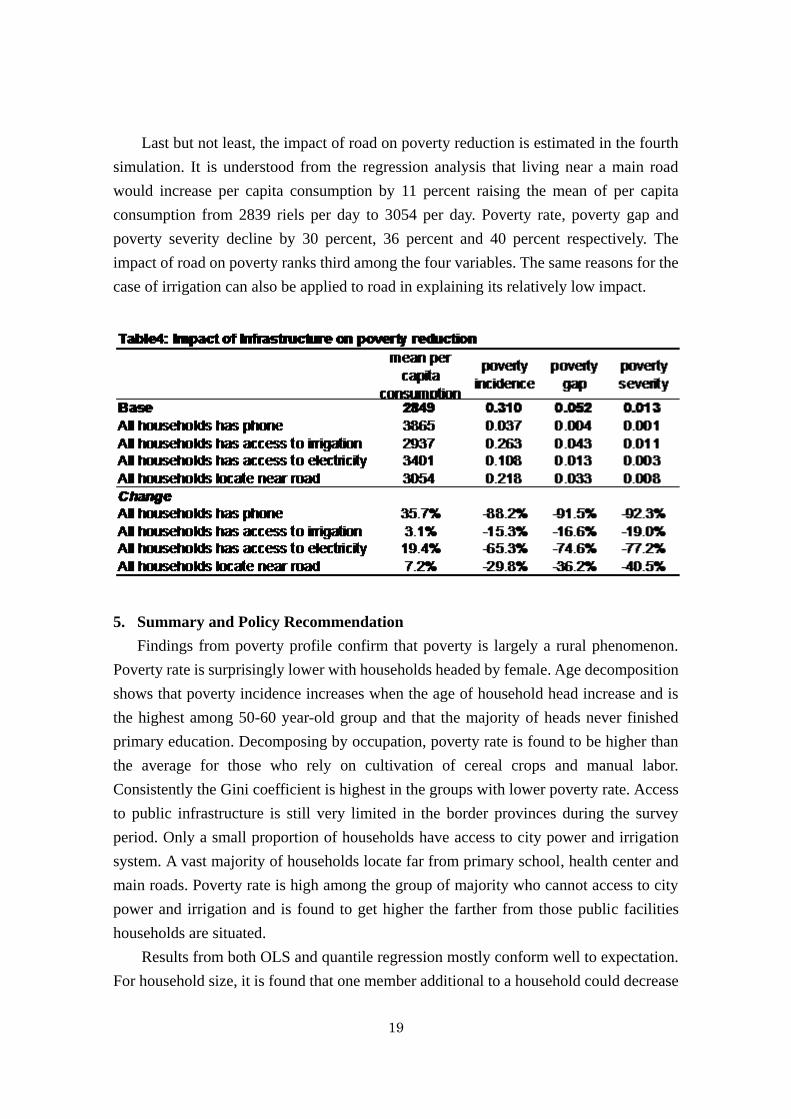
Table 4 presents the simulations of the poverty impact of infrastructure variables

based on the findings from OLS regression analysis with estimation4. For cell phone the

simulation result shows that having cell phone could increase consumption per capita by

36 percent. Poverty incidence would drop dramatically from 31 percent in base point to

only about 4 percent with the presence of cell phone. The effect of cell phone is not

limited to those who live near poverty lines but it runs deeper. The simulation shows that

cell phone also reduce both the depth of poverty and the severity of poverty by about 92

percent.

The second simulation explores the effect of irrigation on poverty reduction. The

result of estimated coefficients indicates that irrigation could raise the mean of

consumption per capita by 3 percent. This can result in alleviating 15 percent of poverty

incidence, 17 percent of poverty gap and 19 percent of poverty severity. The fact that the

effect of irrigation is not as strong as that of cell phone can be explained by the efficiency

of these two variables and the law of diminishing return. Even though irrigation seems

crucial for agricultural production, its quality is not so good. Secondly, since cell phone is

relatively new to people, the marginal return from using it is extremely high.

The third simulation scrutinizes the effect of electricity on poverty reduction. Results

from regression analysis suggest that access to electricity increases the mean of per capita

consumption by 19 percent. The depth of poverty and the severity of poverty are reduced

by 75 and 77 percent respectively. Among all infrastructure variables, the impact of

electricity is the second strongest to reduce poverty following that of cell phones.

19

Last but not least, the impact of road on poverty reduction is estimated in the fourth

simulation. It is understood from the regression analysis that living near a main road

would increase per capita consumption by 11 percent raising the mean of per capita

consumption from 2839 riels per day to 3054 per day. Poverty rate, poverty gap and

poverty severity decline by 30 percent, 36 percent and 40 percent respectively. The

impact of road on poverty ranks third among the four variables. The same reasons for the

case of irrigation can also be applied to road in explaining its relatively low impact.

5. Summary and Policy Recommendation

Findings from poverty profile confirm that poverty is largely a rural phenomenon.

Poverty rate is surprisingly lower with households headed by female. Age decomposition

shows that poverty incidence increases when the age of household head increase and is

the highest among 50-60 year-old group and that the majority of heads never finished

primary education. Decomposing by occupation, poverty rate is found to be higher than

the average for those who rely on cultivation of cereal crops and manual labor.

Consistently the Gini coefficient is highest in the groups with lower poverty rate. Access

to public infrastructure is still very limited in the border provinces during the survey

period. Only a small proportion of households have access to city power and irrigation

system. A vast majority of households locate far from primary school, health center and

main roads. Poverty rate is high among the group of majority who cannot access to city

power and irrigation and is found to get higher the farther from those public facilities

households are situated.

Results from both OLS and quantile regression mostly conform well to expectation.

For household size, it is found that one member additional to a household could decrease

20

per capita consumption by 10 percent. One the other hand, one level higher of education

and one hectare of additional land to household would increase per capita consumption up

to 19 percent and 6 percent respectively. Sanitation, land title, and tractor could increase

per capita consumption by up to 43 percent, 7 percent and 23 percent, respectively. For

the development level variables, being in the border and urban areas could increase per

capita consumption by 15 percent and 30 percent respectively. Finally, the infrastructure

variables, the variables of interest, are found to exert positive impact on consumption.

Phone, irrigation system, electricity and road could increase per capita consumption by

42 percent, 8 percent, 29 percent, and 11 percent respectively.

The simulations to detect the impact of infrastructure variables on poverty produce

encouraging results. Cell phone, irrigation, electricity and road could reduce poverty

incidence by 94 percent, 56 percent, 88 percent and 64 respectively. The effect of

infrastructure is not limited to those who live near poverty lines but run deeper. The

simulation shows that these variables also reduce the depth of poverty by 97 percent, 78

percent, 94 percent, and 82 percent, and decrease the poverty severity by 97 percent, 86

percent, 96 percent and 88 percent, respectively. Among the four infrastructure variables,

cell phone has the hugest impact on poverty reduction followed by electricity, road and

irrigation.

However, the cost of using infrastructure in Cambodia is extremely high (Lundsrom

and Ronnas 2006). Telephone and internet communications is a type of infrastructure for

which the cost is extremely expensive and the quality is low due to oligopoly markets.

Electricity was ranked high as a business constraint. The electricity cost can be decreased,

either by new sources of energy or by importing cheaper energy. Transportation cost is

very high, mainly due to the poor quality of roads. This has been a major problem for

commercialisation of the agricultural sector as well as industrialisation outside Phnom

Penh.

Royal Government of Cambodia has recognized the important role of infrastructure

for economic development. To further advance rural development there is a need to invest

in rural infrastructure. In the National Strategic Development Plan 2006-2010, the

rehabilitation of physical infrastructure include: primary and secondary roads, railways,

airports, ports, irrigation facilities, telecommunications, electricity generation and

distribution networks, etc., receive top priority with maximum attention being paid to

attracting private sector to undertake work on a BOT basis wherever possible.

Based on empirical investigation above, all the four infrastructure variables which

are included in the Rectangular Strategy appear to have strong effects on poverty

reduction. Project design including location of infrastructure investments is critical.

21

Poverty reduction can be hastened if rural roads, irrigation, and rural electrification

interventions are made in locations that are pivotal in terms of distributive and multiplier

effects.

References

Agénor, P-R, A. Izquierdo, and H. Fofack, (2001), ―IMMPA: A Quantitative

Macroeconomic Framework for the Analysis of Poverty Reduction

Strategies,‖ Washington, DC: World Bank.

Ali and E. Pernia, (2003), ―Infrastructure and Poverty Reduction—What is the

Connection?‖ Economics and Research Department, Policy Brief No.13, ADB,

Manila

Anders, Orjan, and Fredrik, (2008), ―Poverty in Rural Cambodia: The Differentiated

Impact of Linkages, Inputs and Access to Land,‖ Asian Economic Papers

Anders and Kokko, (2007), ―Poverty and Land Policy in Cambodia,‖ Stockholm School

of Economics, Working Paper 233.

Asian Development Bank, (1999), ―Fighting Poverty in Asia and Pacific: The

Poverty Reduction Strategy, ADB: Manila

Asian Development Bank, (2001),‖Participatory Poverty Assessment:

Cambodia,‖ Manila.

Asian Development Bank, (2003) ―Assessment of Implementation of Selected

Sectoral Policy Initiatives and Reforms in Cambodia,‖ ADB: Manila

Balisacan, A.M., E.M. Pernia, and A. Asra, (2002), ―Revisiting Growth and Poverty

Reduction in Indonesia: What Do Subnational Data Show? ERD Working Paper

Series No.25, Economics and Research Department, ADB:Manila

Bhattarai, M.,R. Sakhitavadivel, and Intizar Hussain, (2002), ―Irrigation Impacts on

Income Inequality and Poverty Alleviation,‖ International Water Management

Institute Working Paper 39, Colombo

Calderon, C. and L. Serven (2004), ―The Effects of Infrastructure Development on

Growth And Income Distribution‖, Policy Research Working Paper No. 3400,

World Bank, Washingtong, DC.

Chan Sophal and Kim Sedara, (2003), ―Enhancing Rural Livelihoods,‖

Cambodia Development Review, CDRI: Phnom Penh.

CDRI, (2008), ―Rural Land Titling,‖ Cambodia Development Resource Institute,

Phnom Penh

Deaton, Angus, (1997), ―The Analysis of Household Surveys: A Microeconometric

22

Approach to Development Policy,‖ Baltimore, The Johns Hopkins University

Press.

DFID, (2002), ―Making the Connections: Infrastructure for Poverty Reduction,‖

London

Dollar, David and Kraay, Aart (2000), ―Growth is Good for the Poor,‖

Washington DC, World Bank

Don Richardson, Ricardo Ramirez, Moinul Haq, (2000), ―Grameen Telecom’s Village

Phone Progamme in Rual Bangladesh: A Multi-Media Case Study,‖ Canadian

Development Agency.

Ellis, F. & Bahiigwa, G. (2003), ―Livelihoods and Rural Poverty Reduction in Uganda‖

World Development, (31) 997-1013

Fan, S., L.X. Zhang, and X. B. Zhang, (2002), ―Growth, Inequality, and Poverty

Reduction in Rural China: The Role of Public Investments,‖ Research Report 125,

International Food Policy Research Institute, Washington, DC.

CDRI, (2007), ―Moving Out of Poverty? Trends in Community Well-Being and

Household Mobility in Nine Cambodian Villages,‖ Cambodia Development

Resource Institute.

Jalan, J., and M. Ravallion, (2002), ―Geographic Poverty Traps? A Micro Model of

Consumption Growth in Rural China‖, Journal of Applied Econometrics 17(4):

329-46.

John Weiss, (2003), ―Infrastructure Investment for Poverty Reduction: A Survey of

Key Issues,‖ www.adbi.org/cfinfra03/contents.htm

Knowles, James C, (2003) ―Cambodia Poverty Review,‖ Asian Development Bank:

Manila

Kwon, E.K.,(2000) ―Infrastructure, Growth, and Poverty Reduction in Indonesia: A

Cross-Sectional Analysis,‖ Asian Development Bank, Manila

Lord, Montague, (2001), ―Macroeconomic Policies for Poverty Reduction in Cambodia,‖

Final Report to the Asian Development Bank, Manila.

Lubker et al, (2002) ―Growth and the Poor: A Comment on Dollar and Kraay,‖

Journal of International Development, (14) 555-571.

Mankiw, N.G., D. Romer and D. Weil (1992), ―A Contribution to the Empirics of

Economic Growth,‖ Quarterly Journal of Economics, (107): 407-437.

Martin Ravallion, (1996), ―Issues in Measuring and Modelling Poverty‖

The Economic Journal, (106) 1328-1343

Milbourne, R., Otto, G., and Voss, G.(2003), ―Public Investment and Economic Growth,‖

Applied Economics, (35) 527-540

23

Phim Runsinarith, (2004), ―Empirical Study on Economic Growth Effect of Government

Activities in Developing Countries,‖ Master Thesis.

Roger Koenker and Kevin F. Hallock, (2001) ―Quantile Regression,‖

Journal of Economic Perspectives, (15) 143-156

Royal Government of Cambodia, (1994) ―First Five-Year Socioeconomic

Development,‖ Ministry of Planning: Phnom Penh

Royal Government of Cambodia, (1999) ―Cambodia Poverty Index,‖ Ministry

of Planning, UNDP; SIDA, World Bank: Phnom Penh

Royal Government of Cambodia, (2000) ―Governance Action Plan,‖ Ministry of

Planning, Phnom Penh:

Royal Government of Cambodia, (2000) ―Interim Poverty Reduction Strategy

Paper,‖ Ministry of Planning, Phnom Penh

Royal Government of Cambodia, (2001) ―A Pro-Poor Trade Sector Strategy

for Cambodia: A Preliminary Concept Paper,‖ Presented at the Pre-

Consultative Group Donor Meeting, January

Royal Government of Cambodia, (2001) ―First Draft of the Second Five Year,‖

Ministry of Planning, Phnom Penh

Royal Government of Cambodia, (2003) ―Cambodia Millennium Development Goals

Report,‖ CSD/GSCD/PMATU, Phnom Penh, Royal Government of Cambodia

Royal Government of Cambodia, (2004) ―Rectangular Strategy,‖ Phnom Penh

Shinkai Naoko, (2006), ―Infrastructure Development and Poverty Reduction: The Case

of Vietnam,‖ Forum of International Development Studies, Graduation School of

International Studies, Nagoya University

Songco, J., (2002) ―Do Rural Infrastructure Investments Benefit the Poor? World Bank

Working Paper 2796, Washington, DC

UNCTAD, (2004) ―The Least Developed Countries Report, 2004, Linking

International Trade with Poverty Reduction,‖ United Nations: New York

and Geneva

Woolard, I. and Klasen S. (2005), ―Determinants of Income Mobility and Household

Poverty Dynamics in South Africa,‖ Journal of Development Studies (41)

865-897.

World Bank, (1997), ―Infrastructure Strategies in East Asia: The Untold Story,‖

World Bank Working Papers No.17148.

World Bank, (2004), ―Cambodia at the Crossroads – Strengthening

Accontability to Reduce Poverty,‖ Report No. 30636-KH, East Asia and

the Pacific Region

24

World Bank, (2002), ―A Source Book for Poverty Reduction Strategies,‖

Washington DC

World Bank, (2004), ―Making Services Work for the Poor People,‖

Washington DC

World Bank, (2006), ―Cambodia – Poverty Assessment 2006,‖

Phnom Penh

World Bank, (2009), ―Poverty Profile and Trends in Cambodia,2007,‖

Phnom Penh

Xianbin Yao, (2003) ―Infrastructure and Poverty Reduction-Making Markets

Work for the Poor,‖Asian Development Bank, Manila.