Ingegneria Strutturale e Idraulica -...

AAllmmaa MMaatteerr SSttuuddiioorruumm –– UUnniivveerrssiittàà ddii BBoollooggnnaa

DOTTORATO DI RICERCA IN

Ingegneria Strutturale e Idraulica

Ciclo XXIV

Settore Concorsuale di afferenza: 08/B2

Settore Scientifico disciplinare: ICAR 08

TITOLO TESI

Static analysis of functionally graded cylindrical and conical shells or panels using the generalized unconstrained third

order theory coupled with the stress recovery

Presentata da: Luigi Rossetti Coordinatore Dottorato Relatore Chiarissimo Prof. E. Viola Chiarissimo Prof. E. Viola

Esame finale anno 2013

Index Chapter 1.………………………………………………………………………………………...p.1

Sommario ………………………………………………………………………………………….p.1

1.1 General literature trends……………………………………………………………………… .p.2

1.2 The aim of the present work…………………………………………………………………...p.3

1.3 Problem formulation …………………………………………………………………………..p.3

1.3.1 Third order displacement expansion………………………………………………………... p.4

1.3.2 Relations between strains and displacements……………………………………………….p.5

1.3.3 Relations between stresses and strains……………………………………………………….p.7

1.3.4 Internal forces and moment resultants……………………………………………………….p.9

1.3.5 Normal and shear forces……………………………………………………………………p.10

1.3.6 Moments…………………………………………………………………………................p.11

1.3.7 Higher order moments………………………………………………………………….......p.13

1.3.8 Shear forces………………………………………………………………………………...p.14

1.3.9 Equilibrium equations……………………………………………………………………...p.15

1.3.9.1 The first fundamental equilibrium equation……………………………………………...p.22

1.3.9.2 The second fundamental equilibrium equation…………………………………………...p.24

1.3.9.3 The third fundamental equilibrium equation……………………………………………..p.27

1.3.9.4 The fourth fundamental equilibrium equation…………………………………………....p.30

1.3.9.5 The fifth fundamental equilibrium equation……………………………………………...p.33

1.3.9.6 The sixth fundamental equilibrium equation……………………………………………..p.35

1.3.9.7 The seventh fundamental equilibrium equation…………………………………………..p.38

1.4 Equilibrium equations for doubly curved shells……………………………………………...p.40

1.4.1 Stress recovery via GDQ…………………………………………………………………...p.43

Figures…………………………………………………………………………………………….p.44

References………………………………………………………………………………………...p.45

Chapter 2.……………………………………………………………………………………….p.50

Sommario ………………………………………………………………………………………...p.50

2.1. Introduction…………………………………………………………………………………. p.51

2.2. Functionally graded composite cylindrical shell and fundamental system………………….p.54

2.2.1 Fundamental hypotheses……………………………………………………………………p.54

2.2.2 Displacement field and constitutive equations……………………………………………..p.55

2.2.3 Forces and moments resultants……………………………………………………………..p.58

2.2.3.1 Normal and shear forces…………………………………………………………………p.59

2.2.3.2 Moments………………………………………………………………………………….p.59

2.2.3.3 Higher order moments……………………………………………………………………p.60

2.2.3.4 Shear Forces………………………………………………………………………………p.61

2.2.3.5 Higher order shear resultants……………………………………………………..............p.61

2.2.4 Equilibrium equations………………………………………………………………………p.62

2.3 Discretized equations and stress recovery……………………………………………………p.65

2.4. Numerical results…………………………………………………………………………….p.67

2.4.1 Classes of graded materials…………………………………………………………………p.67

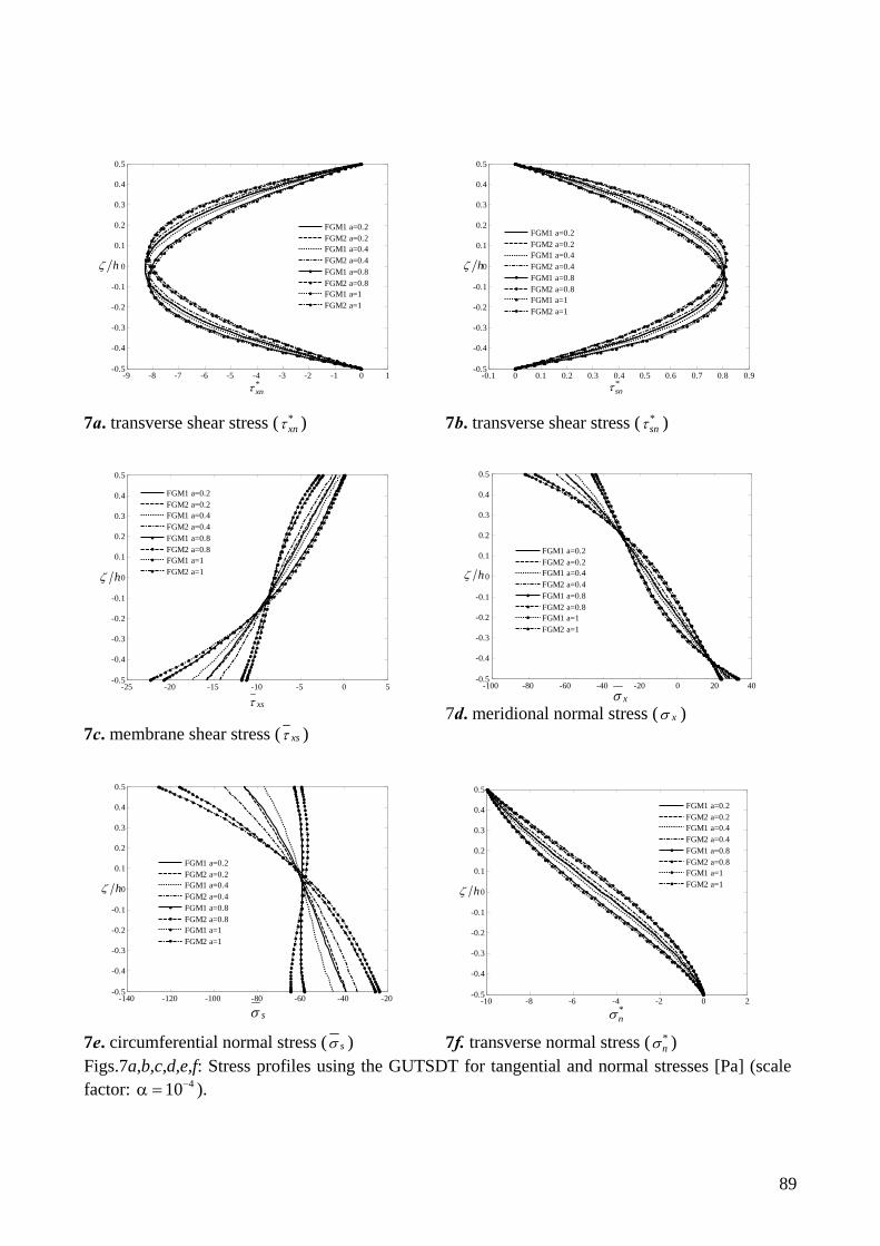
2.4.2 Stress profiles of (1,0,0,p)FGM1 cylindrical panels………………………………………….p.70

2.4.2.1 Generalized and traditional unconstrained theories………………………………………p.70

2.4.3 Stress profiles of (1,1,4,p)FGM1 cylindrical shells…………………………………………….p.71

2.4.3.1 Generalized unconstrained third and first order theories…………………………………p.71

2.4.4 Stress profiles of (1,0.5,2,p)FGM1 cylindrical shells………………………………………….p.71

2.4.4.1 Generalized and traditional unconstrained theories………………………………………p.71

2.4.5 Stress profiles of (a,0.2,3,2)FGM1 and (a,0.2,3,2)FGM2 cylindrical panels……………………p.72

2.4.5.1 The generalized unconstrained theory…………………………………………………..p.72

2.4.6 Stress profiles of (1,0.5,c,2)FGM1 cylindrical panels………………………………………...p.72

2.4.6.1 Generalized unconstrained first and third order theories…………………………………p.72

2.4.7 The stress recovery approach for the generalized unconstrained first and third order

theories……………………………………………………………………………………………p.73

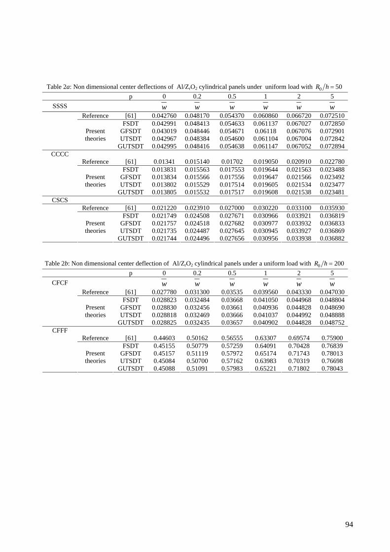
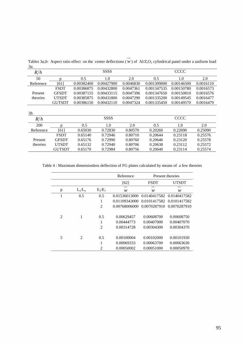
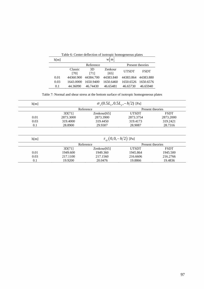
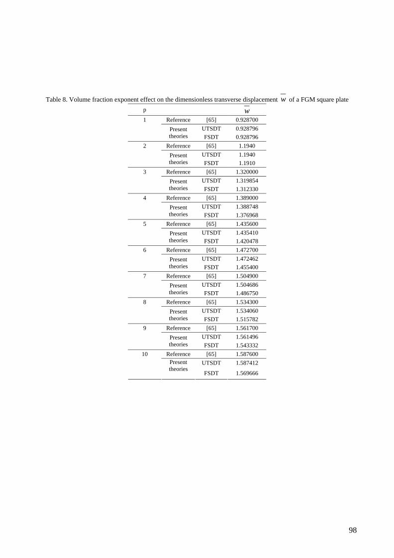
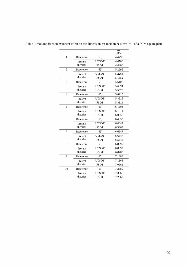
2.5 Literature numerical examples worked out for comparison…………………………………p.73

2.6 Final remarks and conclusion………………………………………………………………...p.75

References………………………………………………………………………………………...p.77

Figures……………………………………………………………………………………………p.83

Tables……………………………………………………………………………………………..p.93

Appendix………………………………………………………………………………………..p.104

Chapter 3.……………………………………………………………………………………...p.109

Sommario ……………………………………………………………………………………….p.109

3.1 Introduction…………………………………………………………………………………p.110

3.2 Functionally graded composite conical shells and fundamental systems…………………...p.117

3.2.1 Fundamental hypotheses…………………………………………………………………..p.117

3.2.2 Displacement field and constitutive equations……………………………………………p.118

3.2.3 Forces and moments resultants……………………………………………………………p.121

3.2.3.1 Normal and shear forces ………………………………………………………………..p.122

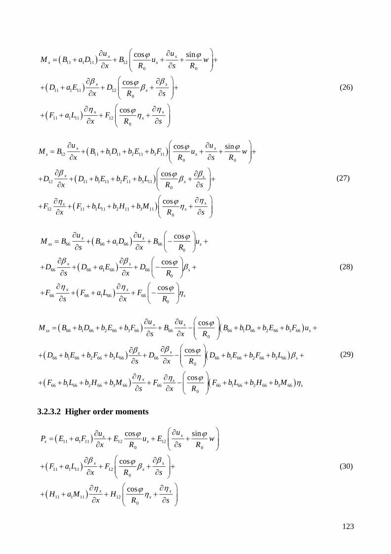
3.2.3.2 Higher order moments………………………………………………………………….p.123

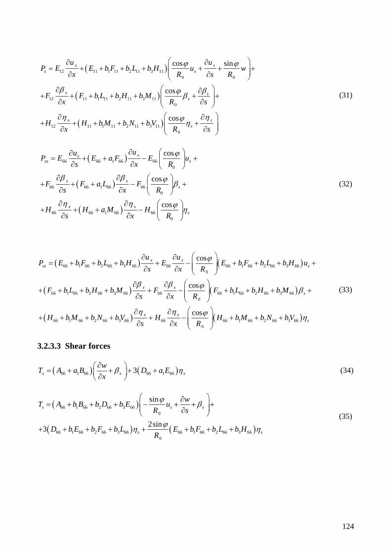
3.2.3.3 Shear forces ……………………………………………………………………………p.124

3.2.3.4 Higher order shear resultants…………………………………………………………...p.125

3.2.4 Equilibrium equations…………………………………………………………………….p.125

3.3 Discretized equations and stress recovery…………………………………………………..p.128

3.4 Stress profiles ……………………………………………………………………………….p.132

3.4.1 The reference configuration……………………………………………………………….p.134

3.4.1.1 The influence of the initial curvature effect with the semi vertex angle……………….p.135

3.4.1.2 The influence of the initial curvature effect with the p - power exponent………………p.136

3.4.1.2.1 Comparisons between the first and third order stress responses with the initial curvature

effect and the p-power exponent………………………………………………………………...p.136

3.4.1.3 The influence of the initial curvature effect with the a – material coefficient………….p.136

3.4.1.3.1 Comparisons between the first and third order stress responses with the initial curvature

effect and the a-material coefficient…………………………………………………………….p.137

3.4.1.4 Comparisons between the first and third order stress responses with the initial curvature

effect and the b-material coefficient…………………………………………………………….p.137

3.4.1.5 The influence of the /L h aspect ratio with the - angle………………………………p.138

3.4.1.5.1 The influence of the /L h aspect ratio with the - angle……………………………..p.138

3.4.1.6 Comparisons between the first and third order recovered and un-recovered transverse stress

distributions……………………………………………………………………………………..p.138

3.4.1.7 The influence of boundary conditions ………………………………………………...p.139

3.4.1.7.1 The influence of the -angle with the initial curvature effect……………………….p.139

3.4.1.7.2 Comparisons between the first and third order stress responses with

the -angle variation and the initial curvature effect…………………………………………...p.139

3.5 Comparison study …………………………………………………………………………..p.140

3.6 Conclusion…………………………………………………………………………………..p.140

References……………………………………………………………………………………….p.141

Figures…………………………………………………………………………………………...p.148

Tables……………………………………………………………………………………………p.167

Appendix………………………………………………………………………………………...p.171

Abstract

A 2D Unconstrained Third Order Shear Deformation Theory (UTSDT) is presented for the

evaluation of tangential and normal stresses in moderately thick functionally graded conical and

cylindrical shells subjected to mechanical loadings. Several types of graded materials are

investigated. The functionally graded material consists of ceramic and metallic constituents. A four

parameter power law function is used. The UTSDT allows the presence of a finite transverse shear

stress at the top and bottom surfaces of the graded shell. In addition, the initial curvature effect

included in the formulation leads to the generalization of the present theory (GUTSDT). The

Generalized Differential Quadrature (GDQ) method is used to discretize the derivatives in the

governing equations, the external boundary conditions and the compatibility conditions. Transverse

and normal stresses are also calculated by integrating the three dimensional equations of

equilibrium in the thickness direction. In this way, the six components of the stress tensor at a point

of the conical or cylindrical shell or panel can be given. The initial curvature effect and the role of

the power law functions are shown for a wide range of functionally conical and cylindrical shells

under various loading and boundary conditions. Finally, numerical examples of the available

literature are worked out.

1

Chapter 1

Third order Shear Deformation Theory

Sommario

Dopo aver analizzato lo stato dell’arte, si è fatta strada l’idea di sviluppare una teoria generale di

deformazione a taglio del terzo ordine di tipo svincolato per gusci/pannelli di rivoluzione a doppia

curvatura, costituiti da uno strato singolo di materiale a stratificazione graduale. Si è operata la

scrittura del modello cinematico a sette parametri indipendenti, delle relazioni tra deformazioni e

spostamenti arricchite dell'effetto della curvatura, delle equazioni costitutive per una lamina singola

in materiale a stratificazione graduale e delle caratteristiche di sollecitazione in funzione degli

spostamenti. Definiti i carichi esterni uniformi di natura trasversale, assiale e circonferenziale, è

stato applicato il principio degli spostamenti virtuali per ricavare le equazioni indefinite di

equilibrio e le condizioni al contorno. Pertanto si è proceduti alla scrittura della equazioni

fondamentali con la sostituzione delle relazioni delle azioni interne espresse in funzione degli

spostamenti, nelle equazioni indefinite di equilibrio. Compiuta la scrittura del sistema fondamentale

si è pervenuti alla soluzione di esso in termini delle sette variabili di spostamento indipendenti,

applicando la tecnica di quadratura differenziale di tipo generalizzato in tutti i punti della superficie

di riferimento del panello/guscio. Dunque è stato possibile determinare le tensioni membranali in un

punto arbitrario appartenente alla superficie di riferimento del panello/guscio ed elaborare poi la

distribuzione di esse lungo lo spessore dell'elemento strutturale. Successivamente con il fine di

pervenire alla determinazione completa del tensore delle tensioni, ovvero delle tensioni trasversali

normale e tagliante, si è operata l'integrazione delle equazioni indefinite di equilibrio sfruttando la

conoscenza delle tensioni membranali, determinate indirettamente dal sistema fondamentale,

sempre utilizzando il metodo generalizzato di quadratura differenziale. Pertanto si è pervenuti alla

determinazione dei profili di tensione trasversale normale e tagliante lungo lo spessore del

panello/guscio. In ambito letterario, il percorso proposto ha degli attributi di autenticità in quanto

consente di calcolare profili di tensione trasversale che soddisfano al pieno le condizioni al

contorno, anche in presenza di carichi taglianti alle superfici di estremità. In tal modo viene

superato uno dei limiti propri della teoria di Reddy che diversamente ritiene nulli a priori i carichi

taglianti alle estremità del panello/guscio.

2

1.1 General literature trends

Two significant classes of two dimensional shell theories can be found in literature: the first based

on the assumed form of the displacement field and the second based on the assumed form of the

stress field. In both cases, the displacement or stress fields are expanded in increasing powers of the

thickness coordinate. Nevertheless, displacement – based theories are more recurrent because they

do not require the strain/stress compatibility condition in addition to the kinematic and equilibrium

equations. It is proved that a third order expansion of the displacement field is optimal because it

gives quadratic variation of transverse strains and stresses, and require no “shear correction factors”

compared to the first order theory, where the transverse strains and stresses are constant through the

shell thickness. A brief overview of research done in third order shell theories is also included in

here.

The simplest and oldest plate theory is the classical Kirchhoff plate theory [1]. The so called

Kirchhoff hypothesis includes the following assumptions: straight lines remain perpendicular to the

reference surface and inextensible after deformation. In this manner both transverse shear and

normal strains [2,3] are neglected. These assumptions in the model simplify the three dimensional

problem to a two dimensional one and the governing equations are expressed in terms of three

displacements of a point on the midsurface. Moreover the theory does not qualify to be called first

order because the first order terms or rotations are not independent of the transverse displacement

component. The theory is very useful in a wide range of problems when thickness is very small

(two orders of magnitude less than the smallest in plane dimension). Transverse shear strains are

also negligible.

The simplest first order shear deformation shell theory (FSDT) often referred to as the Mindlin plate

theory [4-6], is based on the displacement expansion till to the first order, where the first order

terms are the rotations of a transverse normal line and are independent of the transverse

displacement component. The first idea of such expansion can be found in earlier works by Basset

[7], Hencky [8] and Hildebrand et al. [9]. The normality is not invoked and in this way the rotation

are independent of membrane and transverse displacement components and the transverse shear

strains are non zero but independent of out of plane coordinate. This leads to the introduction of

shear correction factors in the evaluation of the transverse shear forces.

Second order and higher order theories relax the Kirchhoff hypothesis further by allowing the

straight lines normal to the midsurface before deformation to become curves. Second order shell

theories are not so diffused because they also require shear correction factors.

The third order theories provide a slight increase in accuracy relative to the FSDT solution, at the

expense of an increase in computational effort and do no require shear correction factors.

3

Several third order plate theories have been developed by different researchers [10-24] but as

pointed by Reddy [21] some of them are claimed to be new whereas they are not new, but only

different in the form of the displacement expansions adopted.

Reddy [19,20] is the first one to develop the equilibrium equations of a third order shell theory with

vanishing tractions for composite structures, using the principle of virtual displacements. By means

of these assumptions, Reddy’s theory reduces the independent displacement components from

seven to five. The theory leads to the accurate reconstruction of the effective transverse shear

components but it excludes the presence of transverse shear loads on the boundary surfaces of the

shell.

1.2 The aim of the present work

In the present work, by moving from Leung’s idea [25] a third order shear deformation theory has

been developed by neglecting the Reddy’s assumptions. The present third order model involves

seven unknown independent parameters and it includes the possible presence of shear uniform loads

in addition to the normal uniform one on the extreme surfaces of composite shell. As in the Reddy’s

theory no correction factor is introduced.

The third order shear deformation theory under discussion is formulated for a single lamina doubly

curved shell of functionally graded material. The seven independent fundamental equations are

achieved by applying the principle of virtual displacements and the fundamental system is solved

by means of the GDQ method [26-62]. By using the GDQ solution in term of the generalized

displacements of points on the reference surface, the membrane profiles of normal and shear

stresses are determined throughout the thickness direction. Then, by considering the three

dimensional equilibrium equations, by discretizing them via the GDQ method and by the

knowledge of the membrane stress components, the transverse profiles of normal and shear stresses

are determined with satisfaction of the boundary conditions at the extreme surfaces. The Reddy’s

model lead to accurate transverse stress profiles by supposing the null values of transverse shear

stress component at the extreme surfaces, whereas the present one in conjunction with the stress

recovery from the three dimensional equations leads to accurate transverse shear stress profiles even

if shear uniform loadings are present on the boundary surfaces.

1.3 Problem formulation

In this study, a single lamina doubly curved shell of functionally graded material represents the

basic configuration of the problem (Fig.1). , s are the coordinates along the meridian and

circumferential directions of the reference surface, respectively. The third orthogonal coordinate to

4

the middle plane along the shell normal is . - coordinate defines the distance of each point

from the shell mid surface 2 2h h and h is the thickness of the shell. The angle between

the extended normal n to the reference surface and the axis of rotation 3x , or the geometric axis

3x of the meridian curve, is defined as the meridian angle . The angle formed by the parallel circle

0 ( )R and the 1x axis is designated as the circumferential angle . The meridian curves and the

parallel circles are represented by the parametric coordinates ( , s ) upon the middle surface of the

shell. The curvilinear abscissa s of a generic parallel is related to the circumferential angle by

the relation 0s R . The horizontal radius 0 ( )R of a generic parallel of the shell represents the

distance of each point from the axis of revolution 3x . bR is the shift of the geometric axis of the

curved meridian 3x with reference to the axis of revolution 3x . The curvature radius R for a shell

of revolution is defined by the relation 0 sinR R . For a general shell of revolution, ,R R ,

0R are all independent of the -angle. The well known equation of Gauss - Codazzi is also

considered : 0 cosdR d R .

The position of an arbitrary point within the shell material is defined by the coordinates

( 0 1 ), s ( 00 s s ) upon the middle surface, and directed along the outward normal and

measured from the reference surface ( 2 2h h ). In the present shell theory, the following

assumptions are taken under consideration in the formulation: (1) the shell deflections are small and

the strains are infinitesimal; (2) the transverse shear deformation is considered to influence the

governing equations. In this manner the normal lines to the reference surface of the shell before

deformation do not remain straight and normal after deformation; (3) the transverse normal strain is

inextensible so that the normal strain is equal to zero; (4) the shell is moderately thick so that the

transverse normal stress could be considered negligible; (5) the linear elastic behavior of composite

materials is assumed; (5) the initial curvature effect is also taken into account.

1.3.1 Third order displacement expansion

Consistent with the assumptions of a moderately thick shell theory reported above, the displacement

field considered in this study is that of the Third order Shear Deformation Theory and can be put in

the following form :

3

3

, , , , ,

, , , , ,

, , ,s s s s

U s u s s s

U s u s s s

W s w s

(1)

5

where u , su , w are the displacement components of points lying on the reference surface ( 0 )

of the shell, along meridional, circumferential and normal directions, respectively. and s are

normal to mid-surface rotations, respectively. and s are the higher order terms. The kinematic

hypothesis expressed by Eq.(1) is enriched by the statement that the shell deflections are small and

strains are infinitesimal, that is ,w s h .

1.3.2 Relations between strains and displacements

The relations of strains for a revolution shell are the followings [64]:

1

1

UW

RR

(2)

00

1cos sin

sin1

UU W

RR

(3)

By considering 0s R , Eq.(3) can be written in the following form:

0 0

1 cos sin

1

ss

UU W

s R R

R

(3.1)

n

W

(4)

11

1 1n

UWR

RR R

R R

(5)

0

0 0

11

1 1n

UWR

RR R

R R

(6)


6

0

0

11

1 1

ssn

UWR

s RR

R R

(6.1)

0

1 1cos

11

UUU

RRRR

(7)


0

1 1 cos

11

ss s

UUU

s RR

RR

(7.1)

By substituting Eq.(1) in Eqs.(2-7.1), relations between strains and displacements become:

31

1

uw

R R

(8)

0 3

cos sin cos1

1cos

uu w

R R

(9)


0 0 0

3

0

cos sin cos

1

1 cos

s s

s

s

uu w

s R R s R

R

s R

(9.1)

2 31 1 1

( 3 2 )1

n

wu

R R RR

(10)

7

2 3

0

1 1 1( 3 2 )

1n

wu

R R RR

(11)


2 31 1

( 3 2 )1

ssn s s s

wu

R s RR

(11.1)

3

3

0

1

1

1cos cos cos

1

u

R R

uu

R R

(12)


3

3

0 0 0

1

1

1 cos cos cos

1

s s ss

s s s

u

R R

uu

s R s R s RR

(12.1)

The transverse normal strain is 0n as in the assumptions.

1.3.3 Relations between stresses and strains

Relations between stresses and strains for a single lamina functionally graded shell are as follows:

11 12

12 22

66

44

55

0

s

s s

n

s s

n n

sn sn

Q Q

Q Q

Q

Q

Q

(13)

where [40,41]:

8

11 22 122 2

66 44 55

( ),

1 ( ) 1

2(1 ( ))

EEQ Q Q

EQ Q Q

(14)

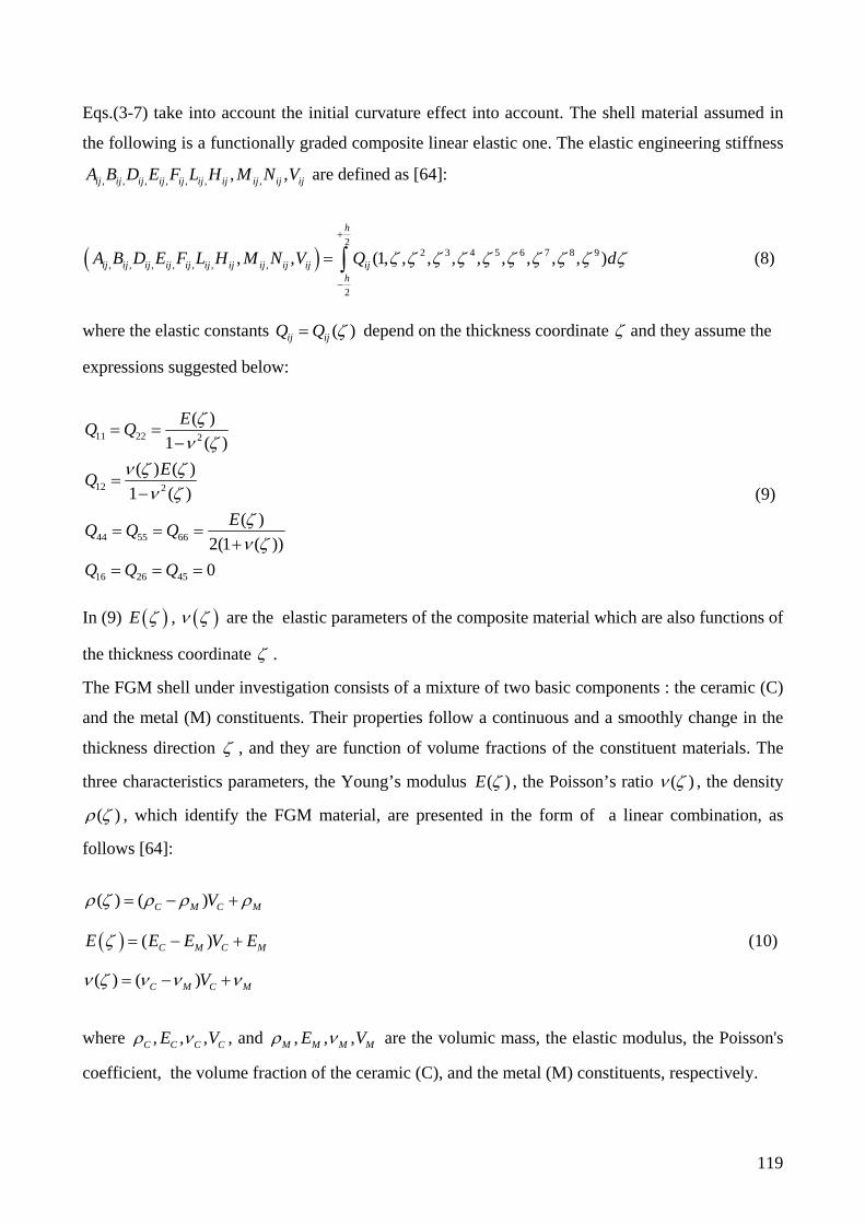
The material properties of the functionally graded lamina vary continuously and smoothly in the

thickness direction and are functions of volume fractions of constituent materials. Young’s

modulus ( )E , Poisson’s ratio and mass density of the functionally graded lamina

can be expressed as a linear combination of the volume fraction:

( )

( )

( )

C M C M

C M C M

C M C M

V

E E E V E

V

(15)

where CV is the volume fraction of the ceramic constituent material, while C , CE , C and

M , ME , M represent mass density, Young’s modulus, Poisson’s ratio of the ceramic and metal

constituent materials, respectively.

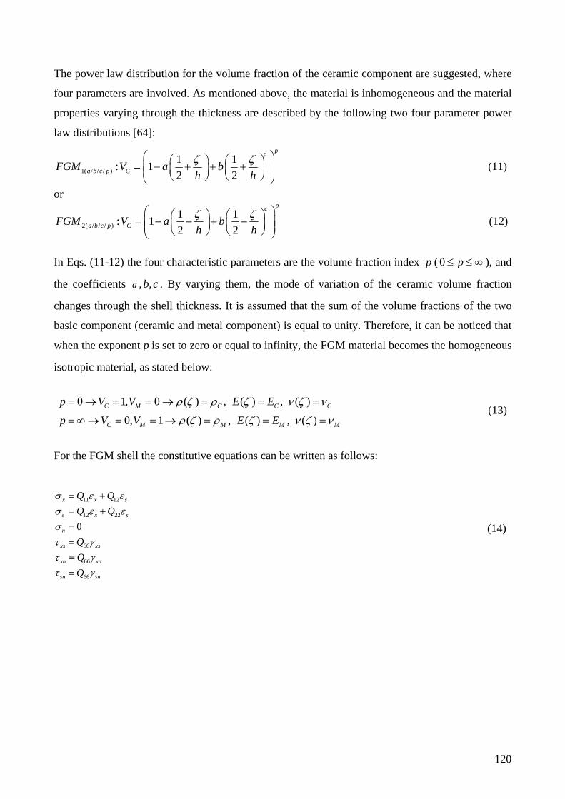
In this work, the ceramic volume fraction CV follows two simple four parameter power law

distributions[40,41]:

1,2( , , , )

1 1: ( ) 1

2 2

pc

a b c p CFGM V a bh h

(16)

where the volume fraction index p ( 0 p ) and the parameters a , b , c determine the material

variation profile along the thickness direction. The elastic engineering constants are written as

follows:

2

2 3 4 5 6 7 8 9, , , , , , ,

2

, , (1, , , , , , , , , )

h

ij ij ij ij ij ij ij ij ij ij ijh

A B D E F L H M N V Q d

(17)

9

1.3.4 Internal forces and moment resultants

Normal forces, moments, and higher order moments, as well as the shear force and higher order

shear force are all defined by the following expressions:

2

3

2

, , (1, , ) 1

h

h

N M P dR

(18)

2

3

2

, , (1, , ) 1

h

s s s sh

N M P dR

(19)

2

3

2

, , (1, , ) 1

h

s s s sh

N M P dR

(20)

2

3

2

, , (1, , ) 1

h

s s s sh

N M P dR

(21)

2

2 3

2

, , (1, , ) 1

h

nh

T Q S dR

(22)

22 3

2

( , , ) (1, , ) 1

h

s s s snh

T Q S dR

(23)

By considering the effect of the initial curvature in the formulation, the stress resultants

, ,s s sN M P are not equal to the stress resultants , ,s s sN M P , respectively. This assumption

derives from the consideration that the ratios / R , / R are not neglected with respect to unity.

The effect of initial curvature is characterized by the following coefficients as firstly done by

Toorani Lakis [63] and then improved by Tornabene [55]:

10

1 2 3 20 0 0

2

1 2 3 20 0 0 0 0

sin 1 1 sin 1 1 sin 1, ,

1 sin sin sin 1 sin sin 1, ,

a a aR R R R R R R R

b b bR R R R R R R R

(24)

1.3.5 Normal and shear forces

By substituting Eqs.(13) in Eqs.(18-21), the following expressions are obtained:

11 1 11 2 11 3 11 12 120

12 11 1 11 2 11 3 110

11 1 11 2 11 3 11 120

12 11 1 11 2 11 3 11 120

12

1 cos

sin 1

1 cos

1 cos

s

s

s

u uN A a B a D a E A u A

R R s

A w A a B a D a E wR R

B a D a E a F BR R

B E a F a L a H Es R R

Es

(25)

12 22 1 22 2 22 3 220

22 1 22 2 22 3 22

22 1 22 2 22 3 22 120

12 22 1 22 2 22 3 220

22 1 22 2 22 3 22

12

1 cos

sin 1

1 cos

1 cos

s

s

s

uN A A b B b D b E u

R R

uA b B b D b E

s

A b B b D b E w A wR R

B B b D b E b FR R

B b D b E b Fs

ER R

22 1 22 2 22 3 220

22 1 22 2 22 3 22s

E b F b L b H

E b F b L b Hs

(26)

11

66 66 1 66 2 66 3 66 660

66 66 1 66 2 66 3 66 660

66 66 1 66 2 66 3 66 660

1 cos

1 cos

1 cos

ss s

ss

ss

u uN A A a B a D a E A u

s R R

B B a D a E a F Bs R R

E E a F a L a H Es R R

(27)

66 1 66 2 66 3 66 66

66 1 66 2 66 3 66 66 1 66 2 66 3 660

66 66 1 66 2 66 3 660

66 1 66 2 66 3 66 66

1

cos

1 cos

1

ss

s

ss

s

u uN A b B b D b E A

s R

A b B b D b E u B b D b E b FR s

B B b D b E b FR R

E b F b L b H Es R

66 1 66 2 66 3 66

0

cossE b F b L b H

R

(28) 1.3.6 Moments


11 1 11 2 11 3 11 12 120

12 11 1 11 2 11 3 110

11 1 11 2 11 3 11 120

12 11 1 11 2 11 3 11 120

12

1 cos

sin 1

1 cos

1 cos

s

s

s

u uM B a D a E a F B u B

R R s

B w B a D a E a F wR R

D a E a F a L DR R

D F a L a H a M Fs R R

Fs

(29)

12

12 22 1 22 2 22 3 220

22 1 22 2 22 3 22

22 1 22 2 22 3 22 120

12 22 1 22 2 22 3 220

22 1 22 2 22 3 22

12

1 cos

sin 1

1 cos

1 cos

s

s

s

uM B B b D b E b F u

R R

uB b D b E b F

s

B b D b E b F w B wR R

D D b E b F b LR R

D b E b F b Ls

FR R

22 1 22 2 22 3 220

22 1 22 2 22 3 22s

F b L b H b M

F b L b H b Ms

(30)

66 66 1 66 2 66 3 66 660

66 66 1 66 2 66 3 66 660

66 66 1 66 2 66 3 66 660

1 cos

1 cos

1 cos

ss s

ss

ss

u uM B B a D a E a F B u

s R R

D D a E a F a L Ds R R

F F a L a H a M Fs R R

(31)

66 1 66 2 66 3 66

66 66 1 66 2 66 3 660

66 1 66 2 66 3 66

66 66 1 66 2 66 3 660

66 1 66 2 66 3 66

66

1 cos

1 cos

1

s

ss

ss

uM B b D b E b F

s

uB B b D b E b F u

R R

D b E b F b Ls

D D b E b F b LR R

F b L b H b Ms

FR

66 1 66 2 66 3 660

cosssF b L b H b M

R

(32)

13

1.3.7 Higher order moments


11 1 11 2 11 3 11 120

12 12 11 1 11 2 11 3 110

11 1 11 2 11 3 11 120

12 11 1 11 2 11 3 11 120

12

1 cos

sin 1

1 cos

1 cos

s

s

s

uP E a F a L a H E u

R R

uE E w E a F a L a H w

s R R

F a L a H a M FR R

F H a M a N a V Hs R R

Hs

(33)

12 22 1 22 2 22 3 220

22 1 22 2 22 3 22

22 1 22 2 22 3 22 120

12 22 1 22 2 22 3 220

22 1 22 2 22 3 22

12

1 cos

sin 1

1 cos

1 cos

s

s

s

uP E E b F b L b H u

R R

uE b F b L b H

s

E b F b L b H w E wR R

F F b L b H b MR R

F b L b H b Ms

HR R

22 1 22 2 22 3 220

22 1 22 2 22 3 22s

H b M b N b V

H b M b N b Vs

(34)

66 66 1 66 2 66 3 66 660

66 66 1 66 2 66 3 66 660

66 66 1 66 2 66 3 66 660

1 cos

1 cos

1 cos

ss s

ss

ss

u uP E E a F a L a H E u

s R R

F F a L a M a N Fs R R

H H a M a N a V Hs R R

(35)

14

66 1 66 2 66 3 66 66

66 1 66 2 66 3 660

66 1 66 2 66 3 66 66

66 1 66 2 66 3 660

66 1 66 2 66 3 66 66

1

cos

1

cos

1

ss

s

s

s

s

u uP E b F b L b H E

s R

E b F b L b H uR

F b L b H b M Fs R

F b L b H b MR

H b M b N b V Hs R

66 1 66 2 66 3 660

cossH b M b N b V

R

(36) 1.3.8 Shear forces

By substituting Eqs.(13) in Eqs.(22,23), the following expressions are obtained:

44 1 44 2 44 3 44

44 1 44 2 44 3 44

44 1 44 2 44 3 44

44 1 44 2 44 3 44 44 1 44 2 44 3 44

1

1

23

T A a B a D a E uR

wA a B a D a E

R

A a B a D a E

D a E a F a L E a F a L a HR

(37)

55 1 55 2 55 3 550

55 1 55 2 55 3 55 55 1 55 2 55 3 55

55 1 55 2 55 3 55 55 1 55 2 55 3 550

sin

2sin3

s s

s

s s

T A b B b D b E uR

wA b B b D b E A b B b D b E

s

D b E b F b L E b F b L b HR

(38)

15

44 1 44 2 44 3 44 44 1 44 2 44 3 44

44 1 44 2 44 3 44

44 1 44 2 44 3 44 44 1 44 2 44 3 44

1 1

23

wQ D a E a F a L u D a E a F a L

R R

D a E a F a L

F a L a H a M L a H a M a NR

(39)

55 1 55 2 55 3 55 55 1 55 2 55 3 550

55 1 55 2 55 3 55 55 1 55 2 55 3 55

55 1 55 2 55 3 550

sin

3

2sin

s s

s s

s

wQ D b E b F b L u D b E b F b L

R s

D b E b F b L F b L b H b M

F b L b H b MR

(40)

44 1 44 2 44 3 44

44 1 44 2 44 3 44

44 1 44 2 44 3 44

44 1 44 2 44 3 44 44 1 44 2 44 3 44

1

1

23

S E a F a L a H uR

wE a F a L a H

R

E a F a L a H

L a H a M a N H a M a N a VR

(41)

55 1 55 2 55 3 55 55 1 55 2 55 3 550

55 1 55 2 55 3 55 55 1 55 2 55 3 55

55 1 55 2 55 3 550

sin

3

2sin

s s

s s

s

wS E b F b L b H u E b F b L b H

R s

E b F b L b H L b H b M b N

H b M b N b VR

(42) 1.3.9 Equilibrium equations

Here we use the principle of virtual displacements to derive the equilibrium equations consistent

with the displacement field equations (1). The principle of virtual displacements can be stated in

analytical form as:

16

2

2

( )

0

h

s s s s n n sn sn s sh

n s s s s

d d p u R d ds p u R d ds

p wR d ds m R d ds m R d ds r R d ds r R d ds

(43) where:

01 1d R d R dR R

(43.1)

and , , , , , ,s n s sp p p m m r r are the external uniform loadings applied on the reference surface.

By introducing Eqs.(8-12.1;13) into Eq.(43) and considering Eqs.(18-23), the following terms of

the integral can be separated as follows:

2

2

0 0 0 0

h

h

d

uN R d d N w R d d M R d d P R d d

(43.2)

2

2

cos sin

cos

cos

h

h

ud N R d d N u R d d N w R d d

M R d d M R d d

P R d d P R d d

(43.3)

17

2

0 0 0

2

cos ( )

( cos )

h

h

ud N R d d M R d d P R d d

uN R d d N u R d d M R d d

M R d d P

( cos )R d d P R d d

(43.4)

2

0 0 0

2

0 0

( )

3 2

h

n nh

wd T u R d d T R d d T R R d d

Q R R d d S R d d

(43.5)

2

0

2

0

sin

3 2 (sin )

h

n nh

wd T u R d d T R d d T R R d d

Q R R d d S R d d

(43.6)

By solving the integrals by parts in Eqs.(43.2-43.6), the resulting expressions are obtained:

0

0 0

N RuN R d d N R u u d d

(43.7)

0

0 0

M RM R d d M R d d

(43.8)

0

0 0

P RP R d d P R d d

(43.9)

18


(43.10)

M RM R d d M R d d

(43.11)

P RP R d d P R d d

(43.12)

0

0 0


(43.13)

0

0 0

M RM R d d M R d d

(43.14)

0

0 0

P RP R d d P R d d

(43.15)


(43.16)

M RM R d d M R d d

(43.17)

P RP R d d P R d d

(43.18)

19

0

0 0

T RwT R d d T R w wd d

(43.19)

T RwT R d d T R w wd d

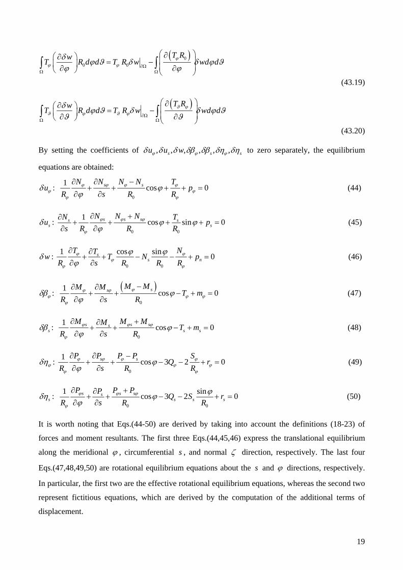
(43.20) By setting the coefficients of , , , , , ,s s su u w to zero separately, the equilibrium

equations are obtained:

u : 0

1cos 0s sN N N N T

pR s R R

(44)

su : 0 0

1cos sin 0s s ss s

s

N N NN Tp

s R R R

(45)

w : 0 0

1 cos sin0s

s n

T NTT N p

R s R R R

(46)

:

0

1cos 0

ssM MM M

T mR s R

(47)

s : 0

1cos 0s s ss

s s

M M MMT m

R s R

(48)

: 0

1cos 3 2 0s sP P P P S

Q rR s R R

(49)

s : 0 0

1 sincos 3 2 0s s ss

s s s

P P PPQ S r

R s R R

(50)

It is worth noting that Eqs.(44-50) are derived by taking into account the definitions (18-23) of

forces and moment resultants. The first three Eqs.(44,45,46) express the translational equilibrium

along the meridional , circumferential s , and normal direction, respectively. The last four

Eqs.(47,48,49,50) are rotational equilibrium equations about the s and directions, respectively.

In particular, the first two are the effective rotational equilibrium equations, whereas the second two

represent fictitious equations, which are derived by the computation of the additional terms of

displacement.

20

Then, substituting the expressions (25-42) for the in-plane meridional, circumferential, and shearing

force resultants , , ,s s sN N N N , the analogous couples , , , , , , ,s s s s s sM M M M P P P P and the

transverse shear force resultants , , , , ,s s sT T Q Q S S , Eqs.(44-50) yield the fundamental system of

equations.

It should be noted that the loadings on the middle surface can be expressed in terms of the loadings

on the upper ( , ,t t ts np p p ) and lower ( , ,b b b

s np p p ) boundary surfaces of the shell by using the static

equivalence principle, as follows:

0 0

0 0

0

sin sin1 1 1 1

2 2 2 2

sin sin1 1 1 1

2 2 2 2

sin sin1 1 1 1

2 2 2

t b

t bs s s

t bn n n

h h h hp p p

R R R R

h h h hp p p

R R R R

h h h hp p p

R R R

0

0 0

0 0

3

0

2

sin sin1 1 1 1

2 2 2 2 2 2

sin sin1 1 1 1

2 2 2 2 2 2

sin1 1

8 2 2

t b

t bs s s

t

R

h h h h h hm p p

R R R R

h h h h h hm p p

R R R R

h h hr p p

R R

3

0

3 3

0 0

sin1 1

8 2 2

sin sin1 1 1 1

8 2 2 8 2 2

b

t bs s s

h h h

R R

h h h h h hr p p

R R R R

(51)

where tp , t

sp , tnp are the meridional, circumferential and normal forces applied to the upper

surface, and bp , bsp , t

np are the meridional, circumferential and normal forces applied to the lower

surface.

The boundary conditions considered in this study are the fully clamped edge boundary condition

(C), the simply supported edge boundary condition (S) and the free edge boundary condition (F).

They assume the following form:

Clamped edge boundary condition (C):

0s s su u w at 0 or 1 00 ,s s (52)

0s s su u w at 0s or 0s s 0 1 (53)

21

Simply supported boundary condition (S):

0u w 0N M P at 0 or 1 00 ,s s (54)

0s s su w 0 s s sN M P at 0s or 0s s 0 1 (55)

Free edge boundary condition (F):

0s s sN N T M M P P

at 0 or 1, 00 s s (56)

0s s s s s s sN N T M M P P

at 0s or 0,s s 0 1 (57)

In the above Eqs.(52-57) boundary conditions, it has been assumed 0 02s R . In order to analyze

the whole shell of revolution, and not a panel, the kinematic and physical compatibility must be

added to the previous external boundary conditions. They represent the condition of continuity

related to displacements and internal stress resultants. Their analytical forms are proposed as

follows:

Kinematic compatibility conditions along the closing meridian 0( 0,2 )s R :

0 0

0 0

0 0

0 0 1

( ,0) ( , ), ( ,0) ( , ),

( ,0) ( , ), ( ,0) ( , ),

( ,0) ( , ), ( ,0) ( , ),

( ,0) ( , )

s s

s s

s s

u u s u u s

w w s s

s s

s

(58)

Physical compatibility conditions along the closing meridian 0( 0,2 )s R :

0 0

0 0

0 0

0 0 1

( ,0) ( , ), ( ,0) ( , ),

( ,0) ( , ), ( ,0) ( , ),

( ,0) ( , ) , ( ,0) ( , ),

( ,0) ( , ),

s s s s

s s s s

s s s s

s s

N N s N N s

T T s M M s

M M s P P s

P P s

(59)

22

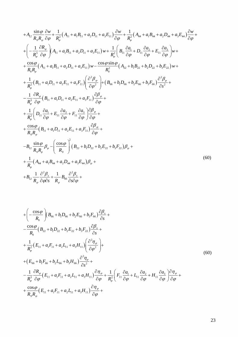
1.3.9.1 The first fundamental equilibrium equation

By substituting Eqs.(25-42) in Eq.(44) the first fundamental equation is written as follows:

2 2

11 1 11 2 11 3 11 66 1 66 2 66 3 662 2 2

31 211 1 11 2 11 3 11 11 11 113 2

11 1 11 2 11 3 110

120

1

1 1

cos

sin

u uA a B a D a E A b B b D b E

R s

R u uaa aA a B a D a E B D E

R R

uA a B a D a E

R R

AR R

2

22 1 22 2 22 3 220

44 1 44 2 44 3 442

2 2

12 66

66 1 66 2 66 3 660

22 1 22 2 22 3 220

cos

1

1 1

cos

cos

s s

s

s

u A b B b D b E uR

A a B a D a E uR

u uA A

R s R s

uA b B b D b E

R s

uA b B b D b E

R s

(60)

23

12 11 1 11 2 11 3 11 44 1 44 2 44 3 442 20

31 211 1 11 2 11 3 11 11 11 113 2

11 1 11 2 11 3 11 20 0

sin 1 1

1 1

cos cos sin

w w wA A a B a D a E A a B a D a E

R R R R

R aa aA a B a D a E w B D E w

R R

A a B a D a E wR R R

22 1 22 2 22 3 22

2 2

11 1 11 2 11 3 11 66 1 66 2 66 3 662 2 2

11 1 11 2 11 3 113

31 211 11 112

11 1 11 2 110

1

1

1

cos

A b B b D b E w

B a D a E a F B b D b E b FR s

RB a D a E a F

R

aa aD E F

R

B a D a E aR R

3 11

2

12 22 1 22 2 22 3 220 0

44 1 44 2 44 3 44

2 2

12 66

sin cos

1

1 1s s

F

B B b D b E b FR R R

A a B a D a ER

B BR s R s

(60)

66 1 66 2 66 3 660

22 1 22 2 22 3 220

2

11 1 11 2 11 3 112 2

2

66 1 66 2 66 3 66 2

111 1 11 2 11 3 11 11 113 2

cos

cos

1

1 1

s

s

B b D b E b FR s

B b D b E b FR s

E a F a L a HR

E b F b L b Hs

R aE a F a L a H F L

R R

3211

11 1 11 2 11 3 110

cos

aaH

E a F a L a HR R

(60)

24

2

12 22 1 22 2 22 3 220 0

44 1 44 2 44 3 44 44 1 44 2 44 3 442

2 2

12 66 66 1 66 2 66 3 660

22 1 22 2 22 30

sin cos

3 2

1 1 cos

cos

s s s

E E b F b L b HR R R

D a E a F a L E a F a L a HR R

E E E b F b L b HR s R s R s

E b F b L b HR

22 0s ps

(60)

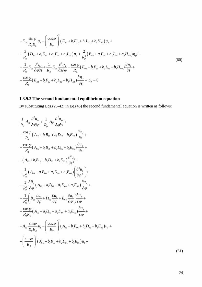
1.3.9.2 The second fundamental equilibrium equation

By substituting Eqs.(25-42) in Eq.(45) the second fundamental equation is written as follows:

2 2

12 66

22 1 22 2 22 3 220

66 1 66 2 66 3 660

2

22 1 22 2 22 3 22 2

2

66 1 66 2 66 3 662 2

66 1 66 2 66 3 663

1 1

cos

cos

1

1

s

s

u uA A

R s R s

uA b B b D b E

R s

uA b B b D b E

R s

uA b B b D b E

s

uA a B a D a E

R

RA a B a D a E

R

31 266 66 662

66 1 66 2 66 3 660

2

66 66 1 66 2 66 3 660 0

2

55 1 55 2 55 3 550

1

cos

sin cos

sin

s

s

s

s s

s

u

uaa aB D E

R

uA a B a D a E

R R

A u A b B b D b E uR R R

A b B b D b E uR

(61)

25

22 1 22 2 22 3 22 120

55 1 55 2 55 3 550

2 2

12 66

22 1 22 2 22 3 220

66 1 66 2 66 3 660

2

22 1 22 2 22 3 22

sin 1

sin

1 1

cos

cos

w wA b B b D b E A

R s R s

wA b B b D b E

R s

B BR s R s

B b D b E b FR s

B b D b E b FR s

B b D b E b F

2

2

66 1 66 2 66 3 662 2

66 1 66 2 66 3 663

31 266 66 662

66 1 66 2 66 3 660

2

66 66 1 66 2 60 0

1

1

1

cos

sin cos

s

s

s

s

s

s

s

B a D a E a FR

RB a D a E a F

R

aa aD E F

R

B a D a E a FR R

B B b D b ER R R

6 3 66

55 1 55 2 55 3 550

sin

s

s

b F

A b B b D b ER

(61)

26

2 2

12 66

22 1 22 2 22 3 220

66 1 66 2 66 3 660

2

22 1 22 2 22 3 22 2

2

66 1 66 2 66 3 662 2

66 1 66 2 66 3 663

1 1

cos

cos

1

1

s

s

s

E ER s R s

E b F b L b HR s

E b F b L b HR s

E b F b L b Hs

E a F a L a HR

RE a F a L a H

R

31 266 66 662

66 1 66 2 66 3 660

2

66 66 1 66 2 66 3 660 0

55 1 55 2 55 3 550

2

55 1 55 2 55 30

1

cos

sin cos

sin3

sin2

s

s

s s

s

aa aF L H

R

E a F a L a HR R


D b E b F b LR

E b F b L bR

55 0s sH p

(61)

27

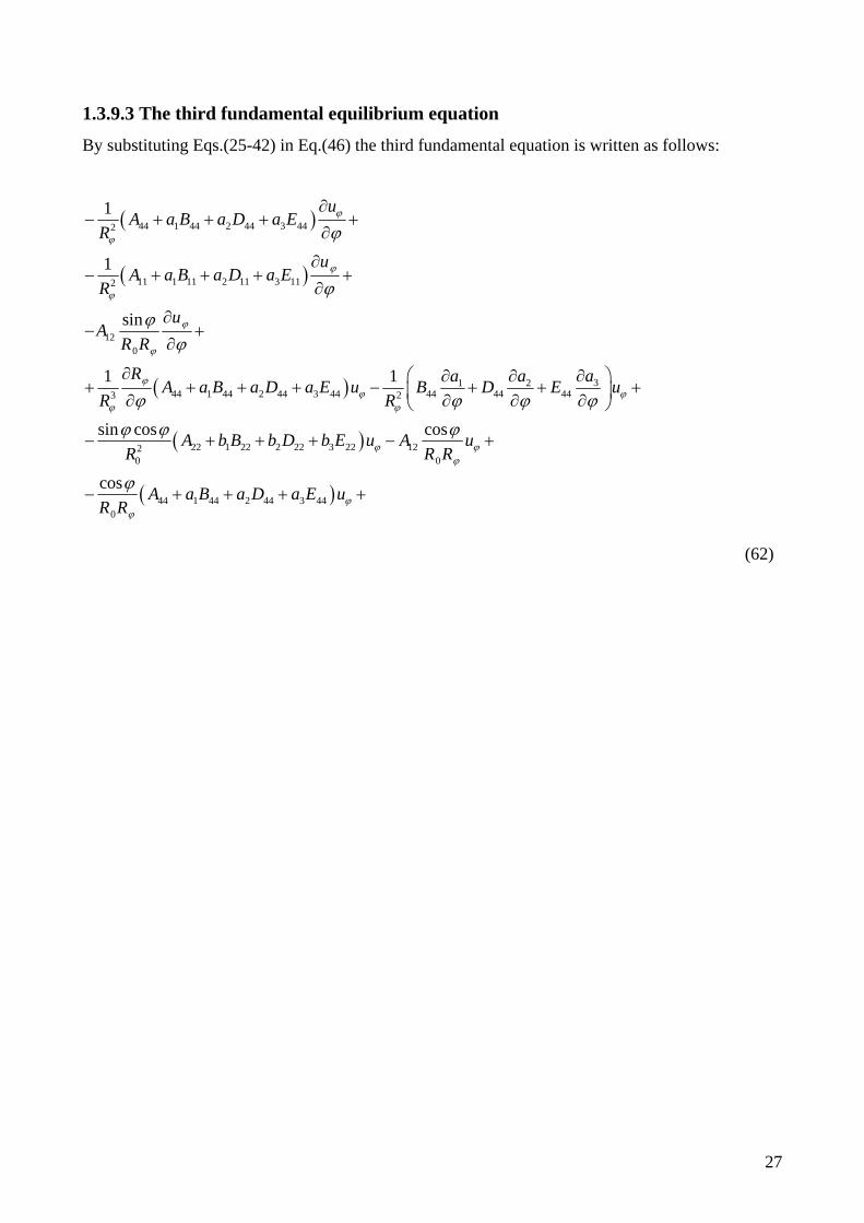
1.3.9.3 The third fundamental equilibrium equation

By substituting Eqs.(25-42) in Eq.(46) the third fundamental equation is written as follows:

44 1 44 2 44 3 442

11 1 11 2 11 3 112

120

31 244 1 44 2 44 3 44 44 44 443 2

22 1 22 2 22 3 22 1220 0

1

1

sin

1 1

sin cos cos

uA a B a D a E

R

uA a B a D a E

R

uA

R R

R aa aA a B a D a E u B D E u

R R

A b B b D b E u AR R

44 1 44 2 44 3 440

cos

uR

A a B a D a E uR R

(62)

28

55 1 55 2 55 3 550

12 22 1 22 2 22 3 220

2

44 1 44 2 44 3 442 2

2

55 1 55 2 55 3 55 2

44 1 44 2 44 3 443

144 42

sin

1 sin

1

1

1

s

s s

uA b B b D b E

R s

u uA A b B b D b E

R s R s

wA a B a D a E

R

wA b B b D b E

sR w

A a B a D a ER

aB D

R

324 44

44 1 44 2 44 3 440

12 11 1 11 2 11 3 1120

2

22 1 22 2 22 3 220

44 1 44 2 44 3 44

11 1 11 2 112

cos

sin 12

sin

1

1

aa wE

wA a B a D a E

R R

A w A a B a D a E wR R R

A b B b D b E wR

A a B a D a ER

B a D a ER

3 11a F

(62)

29

120

31 244 44 44 44 1 44 2 44 3 44

0

12 22 1 22 2 22 3 2220 0

55 1 55 2 55 3 55

12 22 1 22 2 220

sin

1 cos

cos sin cos

1 sin

s

s

BR R

aa aB D E A a B a D a E

R R

B B b D b E b FR R R

A b B b D b Es

B B b D b ER s R

3 22

44 1 44 2 44 3 44 44 1 44 2 44 3 442

11 1 11 2 11 3 11 1220

31 244 44 44 44 1 44 2 44 3 443

2

3 2

1 sin

3 2

2

sb Fs

D a E a F a L E a F a L a HR R

E a F a L a H ER R R

Raa aE F L E a F a L a H

R R

FR

31 244 44 44

44 1 44 2 44 3 44 44 1 44 2 44 3 440 0

12 22 1 22 2 22 3 2220 0

55 1 55 2 55 3 55

55 1 55 2 50

3cos 2cos

cos sin cos

3

2sin

s

aa aL H

D a E a F a L E a F a L a HR R R


D b E b F b Ls

E b F b LR

5 3 55 12

22 1 22 2 22 3 220

1

sin0

ss

sn

b H Es R s

E b F b L b H pR s

(62)

30

1.3.9.4 The fourth fundamental equilibrium equation

By substituting Eqs.(25-42) in Eq.(47) the fourth fundamental equation is written as follows:

2

11 1 11 2 11 3 112 2

2

66 1 66 2 66 3 66 2

11 1 11 2 11 3 113

31 211 11 112

11 1 11 2 11 3 110

120 0

1

1

1

cos

sin cos

uB a D a E a F

R

uB b D b E b F

sR u

B a D a E a FR

uaa aD E F

R

uB a D a E a F

R R

B uR R R

2

22 1 22 2 22 3 22

44 1 44 2 44 3 44

2 2

12 66 66 1 66 2 66 3 660

22 1 22 2 22 3 220

1

1 1 cos

cos

ss s

s

B b D b E b F u

A a B a D a E uR

uu uB B B b D b E b F

R s R s R s

uB b D b E b F

R s

(63)

31

12 11 1 11 2 11 3 1120

44 1 44 2 44 3 44

11 1 11 2 11 3 113

31 211 11 112

11 1 11 2 11 3 110

0

sin 1

1

1

1

cos

cos sin

w wB B a D a E a F

R R R

wA a B a D a E

R

RB a D a E a F w

R

aa aD B F w

R

B a D a E a F wR R

R

22 1 22 2 22 3 222

2

11 1 11 2 11 3 112 2

2

66 1 66 2 66 3 66 2

31 211 1 11 2 11 3 11 11 11 113 2

11 1 11 2 11 3 110

1

1 1

cos

B b D b E b F w

D a E a F a LR

D b E b F b Ls

R aa aD a E a F a L E F L

R R

D a E a F a LR R

(63)

32

2

12 22 1 22 2 22 3 220 0

44 1 44 2 44 3 44

2 2

12 66

66 1 66 2 66 3 660

22 1 22 2 22 3 220

11 1 11 2 11 32

sin cos

1 1

cos

cos

1

s s

s

s

D D b E b F b LR R R

A a B a D a E

D DR s R s

D b E b F b LR s

D b E b F b LR s

F a L a H aR

2

11 2

2

66 1 66 2 66 3 66 2

11 1 11 2 11 3 113

31 211 11 112

11 1 11 2 11 3 110

2

12 22 1 22 20 0

1

1

cos

sin cos

M

F b L b H b Ms

RF a L a H a M

R

aa aL H M

R

F a L a H a MR R

F F b L b HR R R

22 3 22

44 1 44 2 44 3 44 44 1 44 2 44 3 44

2 2

12 66

66 1 66 2 66 3 66 22 1 22 2 22 3 220 0

23

1 1

cos cos0

s s

ss

b M

D a E a F a L E a F a L a HR

F FR s R s

F b L b H b M F b L b H b M mR s R s

(63)

33

1.3.9.5 The fifth fundamental equilibrium equation

By substituting Eqs.(25-42) in Eq.(48) the fifth fundamental equation is written as follows:

2 2

66 12

22 1 22 2 22 3 220

66 1 66 2 66 3 660

2

66 1 66 2 66 3 662 2

2

22 1 22 2 22 3 22 2

66 1 66 2 66 3 663

1 1

cos

cos

1

1

s

s

s

u uB B

R s R s

uB b D b E b F

R s

uB b D b E b F

R s

uB a D a E a F

R

uB b D b E b F

suR

B a D a E a FR

31 266 66 662

66 1 66 2 66 3 660

2

66 66 1 66 2 66 3 660 0

55 1 55 2 55 3 550

22 1 22 2 22 3 22 120

1

cos

sin cos

sin

sin 1

s

s

s s

s

uaa aD E F

R

uB a D a E a F

R R

B u B b D b E b F uR R R

A b B b D b E uR

wB b D b E b F B

R s R

55 1 55 2 55 3 55

2 2

66 12

22 1 22 2 22 3 220

66 1 66 2 66 3 660

1 1

cos

cos

w

s

wA b B b D b E

s

D DR s R s

D b E b F b LR s

D b E b F b LR s

(64)

34

2

66 1 66 2 66 3 662 2

2

22 1 22 2 22 3 22 2

31 266 1 66 2 66 3 66 66 66 663 2

66 1 66 2 66 3 66 660 0

0

1

1 1

cos sin

cos

s

s

ss

ss

D a E a F a LR

D b E b F b Ls

R aa aD a E a F a L E F L

R R

D a E a F a L DR R R R

R

2

66 1 66 2 66 3 66 55 1 55 2 55 3 55

22

66 12

22 1 22 2 22 3 220

66 1 66 2 66 3 660

2

66 1 66 2 66 3 662 2

22 1 22

1 1

cos

cos

1

s s

s

D b E b F b L A b B b D b E

F FR s R s

F b L b H b MR s

F b L b H b MR s

F a L a H a MR

F b L

2

2 22 3 22 2

66 1 66 2 66 3 663

31 266 66 662

66 1 66 2 66 3 660

2

66 66 1 66 2 66 3 660 0

55 1 5

1

1

cos

sin cos

3

s

s

s

s

s s

b H b Ms

RF a L a H a M

R

aa aL H M

R

F a L a H a MR R

F F b L b H b MR R R

D b E

5 2 55 3 55 55 1 55 2 55 3 550

2sin0s s sb F b L E b F b L b H m

R

(64)

35

1.3.9.6 The sixth fundamental equilibrium equation

By substituting Eqs.(25-42) in Eq.(49) the sixth fundamental equation is written as follows:

2 2

11 1 11 2 11 3 11 66 1 66 2 66 3 662 2 2

31 211 1 11 2 11 3 11 11 11 113 2

11 1 11 2 11 3 110

120 0

1

1 1

cos

sin cos

u uE a F a L a H E b F b L b H

R s

R u uaa aE a F a L a H F L H

R R

uE a F a L a H

R R

E uR R R

2

22 1 22 2 22 3 22

44 1 44 2 44 3 44 44 1 44 2 44 3 442

2 2

12 66 66 1 66 2 66 3 660

3 2

1 1 cos ss s

E b F b L b H u

D a E a F a L u E a F a L a H uR R

uu uE E E b F b L b H

R s R s R s

(65)

36

22 1 22 2 22 3 220

12 11 1 11 2 11 3 1120

44 1 44 2 44 3 44

44 1 44 2 44 3 442

11 1 11 2 11 3 113

112

cos

sin 1

3

2

1

1

suE b F b L b H

R s

w wE E a F a L a H

R R R

wD a E a F a L

R

wE a F a L a H

R

RE a F a L a H w

R

FR

31 211 11

11 1 11 2 11 3 110

22 1 22 2 22 3 2220

2

11 1 11 2 11 3 112 2

2

66 1 66 2 66 3 66 2

11 1 11 2 11 3 113

cos

sin cos

1

1

aa aL H w

E a F a L a H wR R

E b F b L b H wR

F a L a H a MR

F b L b H b Ms

RF a L a H a M

R

(65)

37

31 211 11 112

11 1 11 2 11 3 11 120 0

2

22 1 22 2 22 3 22 44 1 44 2 44 3 440

44 1 44 2 44 3 44

2

12

1

cos sin

cos3

2

1 s

aa aL H M

R

F a L a H a M FR R R R

F b L b H b M D a E a F a LR

E a F a L a HR

FR s

2

66

66 1 66 2 66 3 660

22 1 22 2 22 3 220

2

11 1 11 2 11 3 112 2

2

66 1 66 2 66 3 66 2

11 1 11 2 11 3 113

1112

1

cos

cos

1

1

1

s

s

s

FR s

F b L b H b MR s

F b L b H b MR s

H a M a N a VR

H b M b N b Vs

RH a M a N a V

R

aM N

R

3211 11

11 1 11 2 11 3 110

2

12 22 1 22 2 22 3 220 0

44 1 44 2 44 3 44 44 1 44 2 44 3 44

44 1 44 2 44 3 44

cos

sin cos

69

6 4

aaV

H a M a N a VR R

H H b M b N b VR R R

F a L a H a M L a H a M a NR

L a H a M a NR

44 1 44 2 44 3 442

2 2

12 66

66 1 66 2 66 3 660

22 1 22 2 22 3 220

1 1

cos

cos0

s s

s

s

H a M a N a VR

H HR s R s

H b M b N b VR s

H b M b N b V rR s

(65)

38

1.3.9.7 The seventh fundamental equilibrium equation

By substituting Eqs.(25-42) in Eq.(50) the seventh fundamental equation is written as follows:

2 2

66 12 22 1 22 2 22 3 220

66 1 66 2 66 3 660

2

66 1 66 2 66 3 662 2

2

22 1 22 2 22 3 22 2

66 1 66 2 66 3 663

1 1 cos

cos

1

1

1

s

s

s

u u uE E E b F b L b H

R s R s R s

uE b F b L b H

R s

uE a F a L a H

R

uE b F b L b H

suR

E a F a L a HR

31 266 66 662

66 1 66 2 66 3 660

2

66 66 1 66 2 66 3 660 0

55 1 55 2 55 3 550

2

55 1 55 2 55 3 50

cos

sin cos

sin3

sin2

s

s

s s

s

uaa aF L H

R

uE a F a L a H

R R

E u E b F b L b H uR R R

D b E b F b L uR

E b F b L b HR

5

22 1 22 2 22 3 22 120

55 1 55 2 55 3 55 55 1 55 2 55 3 55

2 2

66 12

22 1 22 2 22 3 220

sin 1

2sin3

1 1

cos

su

w wE b F b L b H E

R s R s

w wD b E b F b L E b F b L b H

s R s

F FR s R s

F b L b H b MR s

(66)

39

66 1 66 2 66 3 660

2

66 1 66 2 66 3 662 2

2

22 1 22 2 22 3 22 66 1 66 2 66 3 662 3

31 266 66 66 66 1 66 2 662

0

cos

1

1

1 cos

s

s s

s

F b L b H b MR s

F a L a H a MR

RF b L b H b M F a L a H a M

s R

aa aL H M F a L a M

R R R

3 66

2

66 66 1 66 2 66 3 660 0

55 1 55 2 55 3 55

22

55 1 55 2 55 3 55 66 120

22 1 22 2 22 3 22 66 10 0

sin cos

3

2sin 1 1

cos cos

s

s s

s

s

a N

F F b L b H b MR R R

D b E b F b L

E b F b L b H H HR R s R s

H b M b N b V H bR s R

66 2 66 3 66

2 2

66 1 66 2 66 3 66 22 1 22 2 22 3 222 2 2

31 266 1 66 2 66 3 66 66 66 663 2

66 1 66 2 66 3 660

1

1 1

cos

s s

s s

s

M b N b Vs

H a M a N a V H b M b N b VR s

R aa aH a M a N a V M N V

R R

H a M a N a V HR R

660

2

66 1 66 2 66 3 66 55 1 55 2 55 3 550

55 1 55 2 55 3 55 55 1 55 2 55 3 550 0

2

55 1 55 2 55 3 550

sin

cos9

6sin sin6

sin4 0

s

s s

s s

s s

R R

H b M b N b V F b L b H b MR

F b L b H b M L b H b M b NR R

H b M b N b V rR

(66)

40

1.4 Equilibrium equations for doubly curved shells

The elastic potential energy for a revolution shell can be expressed as follows:

0

11 1

2 n n n n n n R R d d dR R

(67) By assuming the work of external forces equal to zero, the total potential energy becomes equal to

the deformation energy:

eH W (67.1)

The principle of virtual displacement has been applied in order to write the 3D equilibrium

equations.

0 U (67.2)

By considering Eq.(67.2) in Eq.(67), the following relation is obtained:

0sin 0

n n n n n n

R R d d d U

(67.3)

By considering Eqs.(2-7.1) in Eq.(67.3), the total functional can be divided into six terms as

follows:

1 0sin 0V

R R dV U (67.4)

1 0sin 0V

UW R dV U

(67.4.1)

By integrating by parts, the first part of the functional can be expressed as follows:

1 0 0( sin sin 0V

R U R WdV U

(67.5)

41

The second term of the functional is expressed as follows:

2 0sin 0V

R R dV U (67.6)

By considering Eqs.(2-7.1) in Eq.(67.6), the second term becomes:

2 cos sin 0V

UU W R dV U

(67.6.1)

By integrating by parts, the second part of the functional becomes:

2 cos sin 0V

R U R U W dV U

(67.7)

The third term of the functional is the following:

3 0sin 0n n

V

R R dV U (67.8)

By considering Eqs.(2-7.1) in Eq.(67.8), the third term becomes:

3 0sin 0n

V

WR R dV U

(67.8.1)

By means of integration by parts, the third part becomes:

3 0sin 0n

V

R R WdV U

(67.9)

The fourth part of the functional is written as follows:

40

0

1 1cos

sin

sin 0

V

UUU

R R

R R dV U

(67.10)

By integrating by pars, the fourth part is written as follows:

4 0sin

cos 0

V

R U R U

R U dV U

(67.11)

The fifth term of the functional is the following:

42

5 0sin 0n n

V

R R dV U (67.12)

By considering Eqs.(2-7.1) in Eq.(67.12), the fifth term becomes:

5 0

1sin 0n

V

UWR R R dV U

R R

(67.12.1)

By integrating by parts it becomes:

5 0 0

0

sin sin

sin 0

n n

V

n

R W R R U

R U dV U

(67.13)

The sixth term is written as follows:

6 00 0

0

1sin

sin sin

sin 0

n

V

UWR

R R

R R dV U

(67.14)

By integrating by parts, the sixth term becomes:

0

6

sin0

sin

nn

V

R W R R UdV U

R U

(67.15)

By adding the six terms of the potential elastic energy, the total potential energy is expressed as a

function of the virtual displacements and the equilibrium equations can be derived as follows:

The first equilibrium equation is written as follows:

0

0 0

0

1 cos

sin sin

2 sin0

sin

s ns

n

R

R R R s

R R

(68)

43

The second equilibrium equation is written as follows:

0

0 0

0

1 2cos

sin sin

1 2sin0

sin

s s sns

sn

R

R R R s

R R

(69)

The third equilibrium equation is written as follows:

0 0

0

0 0

1 cos 1 sin

sin sin

1 sin0

sin sin

nn s

sn nn

R R R R

R

R s R R

(70)

1.4.1 Stress recovery via GDQ

After solving the 2D problem, the solution of the 3D differential equilibrium equations can be

reached. By means of the GQD solution of the fundamental system (Eqs.(60-66)), the membrane

stresses are correctly estimated using the constitutive equations (Eqs.(13)). Then, by discretizing the

3D equilibrium equations (Eqs.(68-70)) and by the knowledge of membrane stresses and their

derivatives via the GDQ method, the transverse shear and normal stresses can be determined.

44

Figures.

bR

O 'O 1x

2C1C

d

3x '3x

R

1t t

n0 ( )R

n2t t0 ( )R

2x

1xO

Fig.1 Shell geometry: meridional section and circumferential section

45

References.

[1] Kirchhoff G. Uber das Gleichgwich und die Bewegung einer elastischen Scheibe. J Angew

Math 1850; 40: 51-88.

[2] Reddy JN. Mechanics of laminated composite plates and shells: theory and analysis. 2nd ed.

Boca Raton, Florida: CRC Press; 2004.

[3] Reddy JN. Theory and analysis elastic plates and shells. 2nd ed. Boca Raton, Florida: CRC

Press; 2007.

[4] Reissner E. The effect of transverse shear deformation on the bending of elastic plates. J

Appl Mech 1945; 12: A69-77.

[5] Reissner E. Small bending and stretching of sandwich type shells. NACA-TN 1832, 1949.

[6] Mindlin RD. Influence of rotary inertia and shear on flexural motion of isotropic elastic

plates. ASME J Appl Mech 1951; 18: 31-8.

[7] Basset AB. On the extension and flexure of cylindrical and spherical thin elastic shells. Phil

Trans Roy Soc Lond Ser A 1890; 81:433-80.

[8] Hencky H. Uber die Beriicksichtigung der Schubverzerrung in ebenen Platten. Ing Arch

1947; 16: 72-6.

[9] Hildbrand FB., Reissner E., Thomas B. Notes on the foundations of the theory of small

displacements of orthotropic shells. NACA TN-1833, Washington, DC; 1949.

[10]Vlasov BF. Ob uravnieniakh izgiba plastinok (On equations of bending of plates). Doklo

Ak Nauk Azerbeijanskoi SSR 1957;3:955-9. In Russian.

[11] Jemielita G. Techniczna Teoria Plyt Sredniej Grubbosci (Technical theory of plates with

moderate thickness). Rozpruwy nzynierskie (Eng Trans) Polska Akademia Nauk 1975; 23:483-99.

[12] Schmidt R. A refined nonlinear theory of plates with transverse shear deformation. J

Math Soc 1977; 27:23-38.

[13] Krishna Murty AV. Higher order theory for vibration of thick plates. AIAA J 1977;I8:

1823-4.

[14] Lo KH., Christensen RM., Wu EM. A higher order theory of plate deformation-part 1:

homogeneous plates. J Appl Mech, Trans ASME 1977;44(4):663-8.

[15] Lo KH., Christensen RM., Wu EM. A higher order theory of plate deformation-part 2:

laminated plates. J Appl Mech, Trans ASME 1977;44(4):669-76.

[16] Levinson M. An accurate simple theory of the statics and dynamics of elastic plates. Mech

Res Commun 1980;7:343-50.

46

[17] Murthy MVV. An improved transverse shear deformation theory for laminated

anisotropic plates. NASA Technical Paper 1903; 1981-p.1-37.

[18] Kant T. Numerical analysis of thick plates. Comput Methods Appl Mech Eng 1982; 31: 1-

18.

[19] Reddy JN. A simple higher order theory for laminated composite plates. J Appl Mech

1984; 51:745-52.

[20] Reddy JN. A refined nonlinear theory of plates with transverse shear deformation. Int J

Solids Struct 1984; 20:881-96.

[21] Reddy JN. A general non linear third order theory of plates with moderate thickness. Int

J Non Linear Mech 1990;25(6):677-86.

[22] Bhimaraddi A., Stevens LK. A higher order theory for free vibration of orthotropic,

homogeneous, and laminated rectangular plates. J Appl Mech 1984; 51:195-8.

[23] Bose P., Reddy JN. Analysis of composite plates using various plate theories, part. 2:

finite element model and numerical results. Struct Eng Mech 1998;6(7):727-46.

[24] Von Karman Th. Festigkeistprobleme in Mascinenbau. Encyklopadie der Mathematischen

Wissenschaften 1910;4(4):311-385.

[25] Leung AYT. An Unconstrained third order plate theory. Computers & Structures 1991;

40(4): 871-875.

[26] Shu C. Differential quadrature and its application in engineering. Springer 2000.

[27] Bert C., Malik M. Differential quadrature method in computational mechanics. Appl Mech

Rev 1996; 49:1-27.

[28] Liew KM., Han JB., Xiao ZM. Differential quadrature method for thick symmetric cross

ply laminates with first order shear flexibility. Int J Solids Struct 1996; 33: 2647-58.

[29] Shu C., Du H. Free vibration analysis of composites cylindrical shells by DQM. Compos

Part B – Eng 1997; 28B:267-74.

[30] Liew KM, Teo TM. Modeling via differential quadrature method: three dimensional

solutions for rectangular plates. Comput Methods Appl Mech Eng 1998; 159: 369-81.

[31] Liu F-L., Liew KM. Differential quadrature element method: a new approach for free

vibration of polar Mindlin plates having discontinuities. Comput Methods Appl Mech Eng

1999; 179: 407-23.

[32] Viola E., Tornabene F. Vibration analysis of damaged circular arches with varying cross-

section. Struct Integr Durab (SID-SDHM) 2005; 1: 155-69.

[33] Viola E., Tornabene F. Vibration analysis of conical shell shell structures using GDQ

method. Far East J Appl Math 2006; 25: 23-39.

47

[34] Tornabene F. Modellazione e Soluzione di Strutture a Guscio in Materiale Anisotropo.

PhD thesis, University of Bologna, DISTART Department; 2007.

[35] Tornabene F., Viola E. Vibration analysis of spherical structural elements using the GDQ

method. Comput Math Appl 2007; 53: 1538-60.

[36] Viola E., Dilena M., Tornabene F. Analytical and numerical results for vibration analysis

of multi – stepped and multi – damaged circular arches. J Sound Vib 2007; 299: 143-63.

[37] Marzani A., Tornabene F., Viola E. Nonconservative stability problems via generalized

differential quadrature method. J Sound Vib 2008; 315: 176-96.

[38] Tornabene F., Viola E. 2-D solution for free vibrations of parabolic shells using

generalized differential quadrature method. Eur J Mech A – Solid 2008; 27: 1001-25

[39] Alibeigloo A., Modoliat R. Static analysis of cross ply laminated plates with integrated

surface piezoelectric layers using differential quadrature. Compos Struct 2009; 88: 342-53.

[40] Tornabene F. Vibration analysis of functionally graded conical, cylindrical and annular

shell structures with a four parameter power law distribution. Comput Methods Appl Mech

Eng 2009; 198: 2911-35.

[41] Tornabene F., Viola E. Free vibrations of four parameter functionally graded parabolic

panels and shell of revolution. Eur J Mech A – Solid 2009; 28: 991-1013.

[42] Tornabene F., Viola E. Free vibration analysis of functionally graded panels and shells of

revolution. Meccanica 2009; 44: 255-81.

[43] Tornabene F., Viola E., Inman DJ. 2-D differential quadrature solution for vibration

analysis of functionally graded conical, cylindrical and annular shell structures. J Sound Vib

2009; 328: 259-90.

[44] Viola E., Tornabene F. Free vibrations of three parameter functionally graded parabolic

panels of revolution. Mech Res Commun 2009; 36: 587-94.

[45] Yang L., Zhifei S. Free vibration of a functionally graded piezoelectric beam via state

space based differential quadrature. Compos Struct 2009; 87: 257-64.

[46] Alibeigloo A., Nouri V., Static analysis of functionally graded cylindrical shell with

piezoelectric layers using differential quadrature method. Compos Struct 2010; 92: 1775-85.

[47] Andakhshideh A., Maleki S., Aghdam MM. Non linear bending analysis of laminated sector

plates using generalized differential quadrature. Compos Struct 2010; 92: 2258-64.

[48] Hosseini Hashemi Sh., Fadaee M., Es’haghi M. A novel approach for in plane / out of plane

frequency analysis of functionally graded circular /annular plates. Int J Mech Sci 2010;

52:1025-35.

48

[49] Malekzadeh P., Alibeygi Beni A. Free vibration of functionally graded arbitrary straight –

sided quadrilateral plates in thermal environment. Compos Struct 2010; 92: 2758-67.

[50] Sepahi O., Forouzan MR, Malekzadeh P. Large deflection analysis of thermo mechanical

loaded annular FGM plates on nonlinear elastic foundation via DQM. Compos Struct 2010; 92:

2369-78.

[51] Tornabene F., Marzani A., Viola E., Elishakoff I. Critical flow speeds of pipes conveying

fluid by the generalized differential quadrature method. Adv Theor Appl Mech 2010; 3:121-38.

[52] Yas MH, Sobhani Aragh B. Three dimensional analysis for thermoelastic response of

functionally graded fiber reinforced cylindrical panel. Compos Struct 2010; 92: 2391-9.

[53] Tornabene F. Free vibrations of laminated composite doubly – curved shells and panels of

revolution via the GDQ method. Comput Methods Appl Mech Eng 2011; 200: 931-52.

[54] Tornabene F. 2-D GDQ solution for free vibration of anisotropic doubly curved shells and

panels of revolution. Compos Struct 2011; 93: 1854-76.

[55] Tornabene F., Liverani A., Caligiana G. FGM and laminated doubly curved shells and

panels of revolution with a free form meridian: a 2-D GDQ solution for free vibrations. Int J

Mech Sci 2011; 53: 446-70.

[56] Zhao X., Liew KM. Free vibration analysis of functionally graded conical shell panels by

a meshless method. Compos Struct 2011; 93: 649-64.

[57] Tornabene F. Free vibrations of anisotropic doubly curved shells and panels of revolution

with a free form meridian resting on Winkler Pasternak elastic foundations. Compos Struct

2011; 94: 186-206.

[58] Yaghoubshahi M., Asadi E., Fariborz SJ. A higher order shell model applied to shells with

mixed boundary conditions. Proc I Mech E Part C 2011; 225: 292-303.

[59] Tornabene F., Liverani A., Caligiana G. Laminated composite rectangular and annular

plates: a GDQ solution for static analysis with a posteriori shear and normal stress recovery.

Compos Part B – Eng 2012; 43: 1847-72.

[60] Tornabene F., Liverani A., Caligiana G. Static analysis of laminated composite curved

shells and panels of revolution with a posteriori shear and normal stress recovery using

generalized differential quadrature method. Int J Mech 2012; 61: 71-87.

[61] Tornabene F., Liverani A., Caligiana G. General anisotropic doubly curved shell theory: a

differential quadrature solution for free vibrations of shells and panels of revolution with a

free form meridian. J Sound Vib 2012; 331: 4848-69

49

[62] Viola E., Rossetti L., Fantuzzi N. Numerical investigation of functionally graded

cylindrical shells and panels using the generalized unconstrained third order theory coupled

with the stress recovery. Compos Struct 2012; 94: 3736-58.

[63] Toorani MH, Lakis AA. General equations of anisotropic plates and shells including

transverse shear deformations, rotary inertia, and initial curvature effects. J Sound Vib 2000;

237(4): 561-615.

[64] Sokolnikoff IS, Mathematical theory of Elasticity, McGraw-Hill 1956, New York.

50

Chapter 2

Static analysis of functionally graded cylindrical shells and

panels using the generalized unconstrained third order theory

coupled with the stress recovery

Sommario

Dopo l’analisi dello stato dell’arte, si è proceduti con la scrittura di una teoria generale di

deformazione a taglio del terzo ordine di tipo svincolato per gusci/pannelli cilindrici. Si è operata la








spostamenti, nelle equazioni indefinite di equilibrio. Risolto il sistema fondamentale con il metodo

generalizzato di quadratura differenziale, si è pervenuti alla conoscenza dei sette parametri

indipendenti di spostamento, in tutti i punti della superficie di riferimento del panello/guscio

cilindrico. Utilizzando le equazioni costitutive e la soluzione del sistema fondamentale, si è giunti

alla determinazione delle tensioni membranali in un punto arbitrario della superficie di riferimento

del panello/guscio, per poi elaborare la distribuzione di esse lungo lo spessore dell'elemento

strutturale. Per determinare le tensioni trasversali normale e tagliante, si è proceduti con la scrittura

delle equazioni di equilibrio dell’elasticità tridimensionale. Compiuta la discretizzazione di esse con

il metodo di quadratura differenziale di tipo generalizzato, sfruttando la conoscenza delle tensioni

membranali determinate indirettamente dal sistema fondamentale, sono stati calcolati i profili di

tensione trasversale normale e tagliante lungo lo spessore del panello/guscio cilindrico. I profili di

tensione trasversale ottenuti in questo modo soddisfano al pieno le condizioni al contorno anche in

presenza di carichi taglianti alle superfici estreme. In questo modo è stato superato il limite della

teoria di Reddy che assumeva nulli a priori i carichi taglianti alle superfici di estremità. Sono stati

anche discussi l’influenza della curvatura iniziale e del materiale nei profili ottenuti.

51

2.1 Introduction

Composite circular cylindrical shells are extensively used in many engineering applications. As far

as the behaviour of cylindrical shells is concerned, by acting on material type, fiber orientation and

thickness, a designer can tailor different properties of a laminate to suit a particular application.

However, serious shortcomings due to stress concentrations between layers could lead to

delamination failures. In order to overcome the variation of the material properties, the functionally

graded material (FGM) was proposed by Koizumi and Yamanouchi [1,2], characterized by a

smooth and continuous variation from the core to the external surfaces. The possibility to graduate

the material properties through the thickness avoids abrupt changes in the stress and displacement

distributions.

Many researchers have furnished several results in the study of the FGM cylindrical shell [3-32].

Basset [3] presented an overview on the extension and flexure of cylindrical and spherical thin

shells. Bhimaraddi [4] developed a higher order theory for free vibration analysis of circular

cylindrical shells. Obata and Noda [5] studied circular hollow cylinders structured from FGM

material to analyze steady thermal stress at high temperature. Loy et al. [6] reached frequency

spectra of FGM cylindrical shells for simply supported boundary conditions. Hua and Lam [7]

calculated the frequency characteristics of a thin rotating cylindrical shell using the generalized

differential quadrature method. Horgan and Chan [8] analyzed the deformations of a FG cylinder

composed of a compressible isotropic linear elastic material, where the elastic modulus was a power

law function of the radius and the Poisson’s ratio was constant. Pradhan et al. [9] investigated the

vibration characteristics of a FGM shell made up of stainless steel and zirconia, for various

boundary conditions. Liew et al. [10] gave a three dimensional elasticity solution to the free

vibration problem of thick cylindrical shell panels of rectangular platform. Wu et al. [11]

formulated a high order theory to examine the electromechanical behavior of piezoelectric generic

shells with graded material properties in the thickness direction. Zhu et al. [12] discussed the

dynamic stability of functionally graded piezoelectric circular cylindrical shells. Shen and Noda

[13] characterized post buckling phenomena of FGM under combined axial and radial mechanical

loads in high-temperature state. Patel et al. [14] carried out the vibration analysis of a functionally

graded shell using a higher order theory. Najafizadeh and Isvandzibaei [15] used a higher order

shear deformation plate theory to study the vibration of simply supported FG cylindrical shells with

ring supports. Wu and Syu [16] found exact solutions of functionally graded piezoelectric shells

under cylindrical bending. Haddadpour et al. [17] conducted the free vibration analysis of

functionally graded cylindrical shells including thermal effects. Arshad et al. [18] reported the

frequency analysis of functionally graded material cylindrical shells with various volume fraction

52

laws. Iqbal et al. [19] examined the vibration characteristics of FGM circular cylindrical shells filled

with fluid using wave propagation approach. Matsunaga [20] treated a higher order shear

deformation theory in order to assess the natural frequencies and buckling stresses of functionally

graded circular cylindrical shells. Tornabene and Viola [21] and Tornabene [22] dealt with the

dynamic behavior of moderately thick FG cylindrical shells, by using the four parameter power law

distribution. Zhao et al. [23] calculated the static response and free vibration of FGM cylindrical

shells subjected to mechanical or thermomechanical loading using the element-free pk -Ritz

Method. Sobhany Aragh and Yas [24,25] considered the three dimensional analysis of thermal

stresses, static and free vibration analysis of continuously graded fiber reinforced cylindrical shells

by using the generalized power law distribution. In the studies under consideration, the influence of

the power-law exponent and the power-law distribution were investigated. Several symmetric,

asymmetric, and classic profiles were considered. A recent work by Arshad et al. [26] furnished a

detailed analysis of the effects of the exponential volume fraction law on the natural frequencies of

FGM cylindrical shells under various boundary conditions. Alibeigloo [27] estimated the

thermoelastic solution to static deformations of functionally graded cylindrical shell bonded to thin

piezoelectric layers. Sepiani et al. [28] focused on the vibration and buckling analysis of two

layered functionally graded cylindrical shell, considering the effects of transverse shear and rotary

inertia. Nie and Batra [29] evaluated exact solutions and material tailoring for functionally graded

hollow circular cylinders. Alibeigloo and Nouri [30] developed the static analysis of functionally

graded cylindrical shells with piezoelectric layers using differential quadrature method.

Sofiyev [31] presented an analytical study on the dynamic behavior of the infinitely long FGM

cylindrical shell subjected to the combined action of axial tension, internal compressive load and

ring shaped compressive pressure with constant velocity. Sobhani Aragh and Yas [32] studied the

dynamic behavior of four parameter continuous grading fiber reinforced cylindrical panels resting

on Pasternak foundation.

In the last decades, numerous studies have been also conducted on FGM cylindrical shells and

plates, dealing with a variety of subjects such as thermal elasticity [33-35], static bending [36], free

vibration and dynamic response [37,38], buckling and post buckling [39], among others.

Literature review shows that there are quite a few numerical works presenting static analysis of

FGM cylindrical shells. Moreover, the models proposed by different authors in literature are based

on the classical theory, the first order shear deformation theory [33,40-44] and the third order shear

deformation theory by Reddy [45,46].

To the best knowledge of the authors, the literature background on the static analysis of FGM

cylindrical shells by using the unconstrained shear deformation theory of Leung [47] is quite poor.

53

It should be noticed that in Leung’s theory the additional constraint typical of Reddy’s third order

shear deformation theory vanishes [45,46]. In addition, the use of four parameter power law

distributions seems to be absent in the investigation of cylindrical shells, when the initial curvature

effect is included in the model and a GDQ solution [21,22,48,49,50] to the problem is given.

This paper is motivated by this lack of studies and presents a static analysis of thick FGM

cylindrical shells by using an unconstrained third order shear deformation theory. The initial

curvature effect is involved in the analytical formulation as it was included in the first order shear

deformation theory (FSDT) by Toorani and Lakis in the past decade [51] and recently improved by

Tornabene et al. [52]. Furthermore, the stress recovery is worked out.

Firstly, a basic scheme is followed to write the fundamental equilibrium equations. It starts with the

definition of the displacement field which includes higher order terms, the strain components, the

FGM material by means of a four parameter power law distribution, and the elastic engineering

stiffnesses , the stress - strain relations, as well as the relations between the internal actions and the

generalized components of displacement and the definition of external applied loads.

Secondly, seven indefinite equilibrium equations are determined by applying the principle of virtual

displacements. The fundamental equations are obtained by substituting in them the constitutive

equations expressed in terms of generalized components of displacement.

Thirdly, the fundamental equations are discretized via GDQ [53-58] and the differential equilibrium

equations appear in the form of algebraic equations. The boundary conditions also take the

analogous algebraic form. The solution is given in terms of generalized components of

displacement of nodal points on the middle surface domain.

Fourthly, the through-thickness distribution of in plane stress ( , ,x s xs ) are given.

Fifthly, the in plane stress components calculated from the constitutive relations by using the third

order unconstrained theory are compared with those determined via the first order shear

deformation theory, for several types of functionally graded cylindrical shells. Both the transverse

shear stress components ( ,xn sn ) along the thickness direction are determined from the constitutive

equations using the unconstrained first and third order theories, respectively. In order to satisfy the

zero shear conditions on the lateral surfaces which is not imposed a priori in the unconstrained

theory, the transverse shear stress components ( ,xn sn ) are calculated by integrating the 3D

differential equilibrium equations in the thickness direction [20], using the in plane stress

components ( , ,x s xs ) determined via the constitutive relations. The effects of the material power

law function and the initial curvature are discussed and graphically shown in all the numerical

results.

54

Sixthly, the transverse normal stress component ( n ) is carried out by using the recovery

technique, as for the transverse shear stress ( ,xn sn ) components. All the recovered transverse stress

components are improved as reported in [59].

Finally, in order to prove the validity of the present formulation, the numerical examples proposed

by Aghdam et al. [60], Zhao et al. [61], Fereidoon et al. [62] and Ferreira et al. [63,64] are also

considered. The center deflections of isotropic and functionally graded cylindrical panels were

obtained in the present study and compared with the ones reported in [60] and [61]. The vertical

displacements and membrane normal stresses in the central node of functionally graded rectangular

plates were carried out and compared with those reported in [62] and [63,64]. The transverse

displacement component, the membrane normal and transverse shear stresses calculated at an

arbitrary point of functionally graded rectangular plates were compared with the ones derived from

Zenkour [65].

Further publications are reported in [66-73].

2.2. Functionally graded composite cylindrical shell and fundamental system 2.2.1 Fundamental hypotheses

In this paper, a graded composite circular cylindrical shell is considered. 0L , 0R , h denote the

length, the mean radius and the total thickness of the shell, respectively. The position of an arbitrary

point P within the shell is located by the coordinates x 0(0 ),x L s 0 0(0 )s s R upon the

middle surface, and directed along the outward normal n, and measured from the reference

surface ( )2 2h h , as shown in Fig.1.

When the general case of shell of revolution changes into the case under study, the radii of

curvature in the meridional R and circumferential directions R assume the following values:

0,xR R R R (1)

The fundamental hypotheses which characterize the present formulation are the following :

1. the normal strain is inextensible, so the corresponding deformation does not exist;

2. the transverse shear deformation is taken into account in the governing equations, and the

normal lines to the reference surface do not remain straight and normal after deformation;

3. the shell deflections are small and the strains are infinitesimal;

4. the shell is moderately thick, and consequently the normal stress could be negligible;

55

5. the shear correction factor vanishes and the presence of a finite shear transverse strain on the

top and bottom of the cylindrical circular shell is accepted. Thus, the model releases the

additional constrain imposed by the TSDT of Reddy [45,46];

6. the anisotropic material is assumed to be linearly elastic;

7. the initial curvature effect is taken into account. 2.2.2 Displacement field and constitutive equations

The unconstrained third-order shear deformation theory is based on the following representation of

the displacement field across the thickness of the cylindrical shell [47]:

3

3

, , , , ,

, , , , ,

, , ,

x x x x

s s s s

U x s u x s x s x s

U x s u x s x s x s

W x s w x s

(2)

where xU , sU , W are the displacements along the meridional, circumferential and normal

directions, respectively; xu , su are the in-plane displacements, w is the transverse displacement of

a point ,x s on the middle surface. The functions x , s are rotations of the normal to the middle

plane about s and x axes, respectively. The parameters x , s are the higher order terms in

Taylor’s series expansion and represent the higher order transverse cross-sectional deformation

modes.

By substitution of the displacement relations (2) into the strain-displacement equations of the

classical theory of elasticity, the following relations are obtained [72]:

3x x xx

u

x x x

(3)

3

0 0

1

1s s s

s

u w

R s R s s

(4)

2

3xn x x

w

x

(5)

2 3

0 00

1( 3 2 )

1s s

sn s s

u w

R s RR

(6)

56

3 3

0

1

1xs s s x x

xs

uu

x x x s s sR

(7)

Eqs. (3-7) take the initial curvature 01 R effect into account.

The shell material assumed in the following is a functionally graded composite linear elastic one.

The elastic engineering stiffness , , , , , , ,, ,ij ij ij ij ij ij ij ij ij ijA B D E F L H M N V are defined as [21,22]:

2

2 3 4 5 6 7 8 9, , , , , , ,

2

, , (1, , , , , , , , , )

h


A B D E F L H M N V Q d (8)

where the elastic constants ( )ij ijQ Q depend on the thickness coordinate and assume the

expressions suggested below:

11 2

12 11

44 55 66

16 26 45

( )

1 ( )

( )

( )

2(1 ( ))

0

EQ

Q Q

EQ Q Q

Q Q Q

(9)

In (9) E , are the elastic parameters of the composite material which are also functions of

the thickness coordinate .

The FGM shell under investigation consists of a mixture of two basic components : the ceramic (C)

and the metal (M) constituents. Their properties follow a continuous and a smoothly change in the

thickness direction , and they are function of volume fractions of the constituent materials. The

three characteristics parameters, the Young’s modulus E , the Poisson’s ratio ( )v , the density

( ) , which identify the FGM material, are presented in the form of a linear combination, as

follows [21,22]:

( ) ( )

( )

( ) ( )

C M C M

C M C M

C M C M

V

E E E V E

V

(10)

57

where , , ,C C C CE V , and , , ,M M M ME V are the volumic mass, the elastic modulus, the Poisson’s

coefficient, the volume fraction of the ceramic (C), and the metal (M) constituents, respectively.

The power law distributions for the volume fraction of the ceramic component are proposed, where

four parameters are involved. As mentioned above, the material is inhomogeneous and the material

properties varying through the thickness are described by the following four parameter power law

distribution [21,22] :

pc

1(a /b/c/p)

1 1: 1 a b

2 2CFGM Vh h

(11)

or pc

2(a /b/c/p)

1 1: 1 a b

2 2CFGM Vh h

(12)

In Eqs. (11-12) the four characteristic parameters are the volume fraction index p ( 0 p ), and

the coefficients a,b,c. By varying them, the mode of variation of the ceramic volume fraction

changes through the thickness. It is assumed that the sum of the volume fractions of the two basic

components (ceramic and metal component) is equal to unity. Therefore, it can be noticed that when

the exponent p is set to zero or equal to infinity, the FGM material becomes the homogeneous

isotropic material, as stated below:

p 0 1, 0 ( ) , ( ) , ( )

p 0, 1 ( ) , ( ) , ( )

C M C C C

C M M M M

V V E E

V V E E

(13)

For the FGM shell the constitutive equations can be written as follows:

11 12

12 22

66

66

66

0

x x s

s x s

n

xs xs

xn xn

sn sn

Q Q

Q Q

Q

Q

Q

(14)

58

2.2.3 Forces and moments resultants Normal forces, moments, and higher order moments, as well as shear forces and higher order shear

forces are all defined by the following expressions:

2

3

02

, , (1, , ) 1

h

x x x xh

N M P dR

(15)

2

3

2

, , (1, , )

h

s s s sh

N M P d

(16)

2

3

02

, , (1, , ) 1

h

xs xs xs xsh

N M P dR

(17)

2

3

2

, , (1, , )

h

sx sx sx xsh

N M P d

(18)

2

2 3

02

, , (1, , ) 1

h

x x x xnh

T Q S dR

(19)

22 3

2

( , , ) (1, , )

h

s s s snh

T Q S d

(20)

By considering the effect of initial curvature in the formulation, the stress resultants , ,xs xs xsN M P are

not equal to the stress resultants , ,sx sx sxN M P , respectively. This assumption derives from the

consideration that the ratio 0/ R is not neglected with respect to unity. The effect of initial

curvature is emphasized by the following coefficients:

1 1 2 32 30 0 0 0

1 1 1 1; ; ; a b b b

R R R R

(21)

Using Eqs. (3-7), (14-21), the relations which characterize the internal stresses as functions of the displacement parameters can be obtained.

59

2.2.3.1 Normal and shear forces

11 1 11 120

11 1 11 12 11 1 11 12

x sx

x s x s

u u wN A a B A

x s R

B a D B E a F Ex s x s

(22)

12 11 1 11 2 11 3 110

12 11 1 11 2 11 3 11 12

11 1 11 2 11 3 11

x ss

x xs

s

u u wN A A b B b D b E

x s R

B B b D b E b F Ex s x

E b F b L b Hs

(23)

66 66 1 66

66 66 1 66 66 66 1 66

x sxs

s x sx

u uN A A a B

s x

B B a D E E a Fs x s x

(24)

66 1 66 2 66 3 66 66

66 1 66 2 66 3 66 66

66 1 66 2 66 3 66 66

x ssx

x s

x s

u uN A b B b D b E A

s x

B b D b E b F Bs x

E b F b L b H Es x

(25)

2.2.3.2 Moments

11 1 11 120

11 1 11 12 11 1 11 12

x sx

x s sx

u u wM B a D B

x s R

D a E D F a L Fx s x s

(26)

60

12 11 1 11 2 11 3 110

12 11 1 11 2 11 3 11 12

11 1 11 2 11 3 11

x ss

x xs

s

u u wM B B b D b E b F

x s R

D D b E b F b L Fx s x

F b L b H b Ms

(27)

66 66 1 66

66 66 1 66 66 66 1 66

x sxs

x s x s

u uM B B a D

s x

D D a E F F a Ls x s x

(28)

66 1 66 2 66 3 66 66

66 1 66 2 66 3 66 66

66 1 66 2 66 3 66 66

x ssx

x s

x s

u uM B b D b E b F B

s x

D b E b F b L Ds x

F b L b H b M Fs x

(29)

2.2.3.3 Higher order moments

11 1 11 120

11 1 11 12 11 1 11 12

x sx

x s x s

u u wP E a F E

x s R

F a L F H a M Hx s x s

(30)

12 11 1 11 2 11 3 110

12 11 1 11 2 11 3 11 12

11 1 11 2 11 3 11

x ss

x xs

s

u u wP E E b F b L b H

x s R

F F b L b H b M Hx s x

H b M b N b Vs

(31)

66 66 1 66

66 66 1 66 66 66 1 66

x sxs

x s x s

u uP E E a F

s x

F F a L H H a Ms x s x

(32)

61

66 1 66 2 66 3 66 66

66 1 66 2 66 3 66 66

66 1 66 2 66 3 66 66

sxsx

x s

x s

uuP E b F b L b H E

s x

F b L b H b M Fs x

H b M b N b V Hs x

(33)

2.2.3.4 Shear Forces

66 1 66 66 1 66 66 1 663x x x

wT A a B A a B D a E

x

(34)

66 1 66 2 66 3 660

66 1 66 2 66 3 66

66 1 66 2 66 3 66 66 1 66 2 66 3 660

23

ss

s

s

u wT A b B b D b E

R s

A b B b D b E


(35)

2.2.3.5 Higher order shear resultants

66 1 66 66 1 663x x x

wQ D a E F a L

x

(36)

66 1 66 2 66 3 660

66 1 66 2 66 3 66 66 1 66 2 66 3 660

23

ss

s s

u wQ D b E b F b L

R s

D b E b F b L F b L b H b MR

(37)

66 1 66 66 1 663x x x

wS E a F L a H

x

(38)

66 1 66 2 66 3 660

66 1 66 2 66 3 66 66 1 66 2 66 3 660

23

ss s

s

u wS E b F b L b H

R s

L b H b M b N H b M b N b VR

(39)

62

2.2.4 Equilibrium equations Here we use the principle of virtual displacements to derive the equilibrium equations consistent


analytical form as:

2

2

( )

0

h

x x s s xs xs xn xn sn sn x x s sh

n x x s s x x s s

d d p u dxds p u dxds

p wdxds m dxds m dxds r dxds r dxds

(40)

where:

00

1d R d dxR

and , , , , , ,x s n x s x sp p p m m r r are the external loads applied on the reference surface. Introducing Eqs.

(3-7) into Eq.(40), and integrating the resulting expressions by parts, and setting the coefficients of

, , , , , ,x s x s x su u w to zero separately, the following equations of equilibrium are

obtained:

xu : 0x sxx

N Np

x s

su : 0

0s xs ss

N N Tp

s x R

w : 0

0x s sz

T T Np

x s R

x : 0x sxx x

M MT m

x s

(41)

s : 0s xss s

M MT m

s x

x : 3 0x sxx x

P PQ r

x s

s : 0

3 2 0s xs ss s

P P SQ r

s x R

It is worth noting that Eqs.(41) are derived by taking into account the definitions (15-20) of forces

and moment resultants. The first three Eqs.(41) express the translational equilibrium along the

meridional x , circumferential s , and normal direction, respectively. The last four Eqs.(41) are

rotational equilibrium equations about the s and x directions, respectively. In particular, the first

63

two are the effective rotational equilibrium equations, whereas the second two represent fictitious

equations, which are derived by the computation of the additional terms of displacement.


force resultants , , ,x s xs sxN N N N , the analogous couples , , , , , , ,x s xs sx x s xs sxM M M M P P P P and the

transverse shear force resultants , , , , ,x s x s x sT T Q Q S S , Eqs.(41) yield the fundamental system of

equations:

11 12 13 14 15 16 17

21 22 23 24 25 26 27

31 32 33 34 35 36 37

41 42 43 44 45 46 47

51 52 53 54 55 56 57

61 62 63 64 65 66 67

71 72 73 74 75 76 77

x

s

x

s

x

s

R R R R R R R u

R R R R R R R u

R R R R R R R w

R R R R R R R

R R R R R R R

R R R R R R R

R R R R R R R

x

s

n

x

s

x

s

p

p

p

m

m

r

r

(42)

where the explicit forms of the equilibrium operators ijR , , 1,...,7i j are listed in Appendix A.

It can be noticed that the analytical expressions of most of the equilibrium operators in (42) are

characterized by the presence of the coefficients 1 1 2 3, , ,a b b b (21), which incorporate the effect of the

initial curvature, as declared above. By putting 1 1 2 3 0 a b b b , the effect of initial curvature

can be neglected.


on the upper and lower surfaces of the shell as follows:

0 0

1 12 2

t bx x x

h hp p p

R R

0 0

1 12 2

t bs s s

h hp p p

R R

0 0

1 12 2

t bn n n

h hp p p

R R

0 0

1 12 2 2 2

t bx x x

h h h hm p p

R R

(43)

0 0

1 12 2 2 2

t bs s s

h h h hm p p

R R

64

3 3

0 0

1 18 2 8 2

t bx x x

h h h hr p p

R R

3 3

0 0

1 18 2 8 2

t bs s s

h h h hr p p

R R

where t

xp , tsp , t

np are the meridional, circumferential and normal forces applied to the upper

surface, and bxp , b

sp , tnp are the meridional, circumferential and normal forces applied to the lower

surface.


(C), the simply supported edge boundary condition (S) and the free edge boundary condition (F).

They assume the following form:


0x s x s x su u w at 0x or 0x L 00 ,s s (44)

0x s x s x su u w at 0s or 0s s 00 x L (45)

Simply supported boundary condition (S):

0x x xu w 0 x x xN M P at 0x or 0x L 00 ,s s (46)

0s s su w 0 s s sN M P at 0s or 0s s 00 x L (47)


0 x xs x x xs x xsN N T M M P P

at 0x or 0,x x 00 s s (48)

0 s sx s s sx s sxN N T M M P P

at 0s or 0,s s 00 x L (49)

In the above (44)-(49) boundary conditions, it has been assumed 0 02s R . In order to analyze the

whole shell of revolution, and not a panel, the kinematic and physical compatibility must be added

to the previous external boundary conditions. They represent the condition of continuity related to

displacements and internal stress resultants. Their analytical forms are proposed as follows:


65

0 0

0 0

0 0

0 0

( ,0) ( , ), ( ,0) ( , ),

( ,0) ( , ), ( ,0) ( , ),

( ,0) ( , ), ( ,0) ( , ),

( ,0) ( , ) 0

x x s s

x x

s s x x

s s

u x u x s u x u x s

w x w x s x x s

x x s x x s

x x s x L

(50)


0 0

0 0

0 0

0 0

( ,0) ( , ), ( ,0) ( , ),

( ,0) ( , ), ( ,0) ( , ),

( ,0) ( , ) , ( ,0) ( , ),

( ,0) ( , ), 0

s s sx sx

s s s s

sx sx s s

sx sx

N x N x s N x N x s

T x T x s M x M x s

M x M x s P x P x s

P x P x s x L

(51)

2.3 Discretized equations and stress recovery

The generalized differential quadrature method (GDQ) [53-58] is used to discretize the derivatives

in the governing equations (42), as well as the external boundary conditions and the compatibility

conditions. In this paper, the Chebyshev-Gauss-Lobatto grid distribution is adopted, where the

coordinates of grid points along the reference surface are identified by the following relations:

1 00

0

11 cos

1 2

1,2,...., , 0,

i

x xix x

N

i N for x L

(52)

0

0

11 cos ,

1 2

1,2,...., , 0,

j

sjs

M

j M for s s

where N , M are the total number of sampling points which discretize the domain in x and

s directions, respectively. This particular choice of the C-G-L sampling points rule with respect to

the others suggested in literature is justified by the tested efficiency of the GDQ technique.

By writing the fundamental equilibrium equations (42) by means of GDQ technique, the following

matrix form is obtained:

bb bd b b

db dd d d

K K δ p

K K p (53)

66

In the present formulation the subscripts b and d stand for boundary and domain, respectively. The

b -equations define the external boundary conditions and compatibility conditions written on the

constrained edges of the cylindrical shell, and the d -equations represent the scripture of the

fundamental equations at the points which belong to the domain. The solution procedure by means

of the GDQ technique is implemented with the support of a MATLAB code.

According to the Reddy’s constrained theory, the transverse shear stresses satisfy a priori the zero

shear condition on the upper and lower surfaces of the graded cylindrical shell. As it is well known,

and differently from the constrained theory by Reddy, the transverse shear stress determined from

the 2D-Unconstrained Theory of first and third order does not satisfy the zero shear condition on the

lateral surfaces of the cylindrical shell. A possible approach for solving this difficulty is to recovery

the out of plane shear stress using 3D-equilibrium equations. In the case of plates, a general

presentation of the stress recovery problem is reported in [59].

Using the stationary principle of total potential energy, the 3D elastic equilibrium equations for a

functionally graded cylindrical shell are written as follows:

0

0 0

1xn x xsxn

R

R x R s

(54)

0

0 0

2sn xs ssn

R

R x R s

(55)

0

0 0 0

1 1

1n xn sn

n sR

R x R R s

(56)

By the knowledge of the membrane stresses ( , ,x s xs ) and their derivatives in all the points of the

3D cylindrical shell, the present equations (54-56) of the first order can be solved via the GDQ

along the thickness direction. The C-G-L grid distribution is selected for the grid points m along

the thickness direction:

11 cos , 1, 2.., , ,

1 2 2 2 2mm h h h h

m TT

(57)

By imposing the boundary conditions at the bottom surface of the shell, equations (54) and (55) are

written via the GDQ method in the algebraic form and solved in terms of ,xn sn .

( )(1) 0( )

0 0( ) ( )1

( 1) ( )

2,3.....

Txn ijm x xs

xn ijkmkm mijm ijmk

xn ij x ij

R

R x R s m T

p

(58)

67

(1) 0( ) ( )

0 0( ) ( )1

( 1) ( )

2

2,3....

Txs s

sn ijk sn ijmmkm mijm ijmk

sn ij s ij

R

R x R s m T

p

(59)

The shear stress distributions ,xn sn carried out by the linear systems (58) and (59) do not satisfy

the boundary condition at the top surface of shell structure. Consequently, the transverse shear

stress representations are improved via the refinement suggested by Auricchio and Sacco [66] and

Tornabene et al. [59], in the following manner:

( ) ( )( ) ( ) 2

x ij xn ijTrxn ijm xn ijm m

p h

h

(60)

( ) ( )( ) ( ) 1, 2.....

2s ij sn ijTr

sn ijm sn ijm m

p hm T

h

Finally, the transverse normal stress n profiles are derived by solving the equation (56) via the

GDQ method:

( ) ( )(1) 0( )

0 0 01 ( ) ( )

( 1) ( )

2,3....

T r rn ijm s ijmxn sn

n ijkmkm m mk ijm ijm

n ij n ij

R

R x R s R m T

p

(61)

In order to satisfy the boundary condition at the top surface, the n distributions are also corrected

as follows:

( ) ( )( ) ( ) 1, 2....

2n ij n ijTr

n ijm n ijm m

p hm T

h

(62)

2.4 Numerical results 2.4.1 Classes of graded materials In this numerical study, the static analysis of FGM cylindrical shells is conducted and the through

the thickness stress distributions are furnished. The theoretical formulations are based on two shear

deformation models: the generalized unconstrained third (GUTSDT) and first order (GFSDT) shear

deformation theories. They are labeled as generalized because they are enriched by the initial

curvature effect. The stress recovery is also proposed in order to define the correct profile of the

68

transverse shear and normal stress profiles, by the knowledge of the membrane stress components

derived from the 2D shear deformation model. In this manner the shear effect is definitely

improved. The numerical analysis is done by means of the GDQ numerical technique.

The basic constituents of FGM materials are taken to be zirconia (ceramic component) and

aluminum (metal component). Young’s modulus and Poisson’s ratio for the zirconia are

168CE GPa , 0.3C , and for the aluminum are 70ME GPa , 0.3M , respectively. The

ceramic volume fraction is varied by means of the four parameter power law distribution [21,22].

The main objectives of the numerical study reported in this section are the followings:

1. to study the role of the four parameters of the power law function for various classes of

graded materials;

2. to compare the numerical results via the unconstrained third order model with those via the

first order one;

3. to clarify the influence of the initial curvature effect in the numerical analysis, developed

herein;

4. to emphasize the key role of the stress recovery technique in determining the transverse

normal and tangential stress components.

In order to characterize the effect of the volume fraction gradation as a function of the material

coefficients, eight types of graded materials are investigated. In Fig.2a the distributions of the

ceramic volume fraction CV across the thickness for a wide range of p -values are presented for the

(1,0,0,p)FGM1 class. It should be noticed that the lower surface 0.5h of the composite

structure is fully ceramic, and the top surface 0.5h is purely metallic. For 0.1 p 2

(Fig.2a), the material composition is continuously graded throughout the thickness. Differently, for

p 5 the ceramic volume fraction gradually changes only for 0.5 0.25h , and for the remaining

thickness it attains a null value. For p 8 , the ceramic volume fraction is continuously graded from

the bottom surface to the middle layer, and for the rest it has a null value. For p 50,100 , the

variation of the ceramic volume fraction is very restricted to the layers which are closer to the

bottom one, and moving away the ceramic volume fraction becomes equal to zero. In Fig.2b, the

distributions of the ceramic volume fraction are shown for the (1,1,4,p)FGM1 class for several p-values

[22]. All the (1,1,4,p)FGM1 composite shells are fully ceramic at the top and bottom surfaces. For

p 1 the ceramic volume fraction remains higher than 50%, whereas for p 2 the ceramic

69

volume fraction CV has the analogous trend but it reaches values lower than 50%. For 0 0.5h

and p 1 , the ceramic volume fraction rapidly increases and it remains higher than 50%. For

p 0.05 , the distribution of the ceramic volume fraction is quasi ceramic. For p 20,50 the

graded microstructure only belongs to the lower and upper layers of the (1,1,4,p)FGM1 cylindrical

shell, and reveals an homogeneous composition rich in the metal constituent inside the composite

structure. In Fig.2c, the ceramic volume fraction of the (1,0.5,2,p)FGM1 graded material is plotted

versus the dimensionless shell thickness [22]. The bottom surface of the composite shell structure is

fully ceramic for all the p - values. The top surface is made of a mixture of ceramic and metallic

constituents for p 0.6,2,5 , with increasing metallic content with respect to the ceramic one,

respectively. For p 10,20,50 the ceramic volume fraction is continuously graded from the bottom

surface till h variable, respectively, equal to 0.25, -0.25, -0.375. Consequently, the resulting

composite material for p 50 is prevalently metallic. In Fig.2d, the distributions of the ceramic

volume fraction across thickness for several a -values are presented for the (a,0.2,3,2)FGM1 class

[24,32]. It appears that the bottom surface of the composite structure is purely ceramic, and the top

surface changes its composition with the variation of the a -parameter. For a 0.2 the top surface of

the (a,0.2,3,2)FGM1 cylindrical shell is also ceramic. By varying the a -parameter from 0.3 to 1, the

top surface becomes a mixture of ceramic and metallic constituents. In particular, with the increase

of a , the top surface becomes richer and richer of the metallic component. In Fig.3a, the

distributions of the ceramic volume fraction across the thickness for several a -values are presented

for the (a,0.2,3,2)FGM2 class. In contrast with the previous case, it appears that the top surface of the

composite structure is purely ceramic, and the bottom surface changes its composition with the

variation of the a -parameter. For a 0.2 the bottom surface of the (a,0.2,3,2)FGM2 cylindrical shell is

also ceramic. By varying the a -parameter from 0.3 to 1, the bottom surface is made from a mixture

of ceramic and metallic constituents. In particular, with the increase of a , the bottom surface

becomes richer and richer of the metallic component. For all the a -values, the ceramic volume

fraction is continuously graded throughout the shell thickness. In Fig.3b, the distributions of the

ceramic volume fraction across the thickness for several a -values are presented for the

(0,b,2,1)FGM2 class [24,32]. It appears that the top surface of the composite structure is purely

ceramic, and the bottom surface changes its composition with the variation of the b -parameter. By

varying the b -parameter from -0.2 to -0.9, the bottom surface is made from a mixture of ceramic

and metallic constituents. In particular, with the decrease of b , the bottom surface becomes richer

70

and richer of the metallic component. For b 1 the bottom surface is purely metallic. From Figs.

3a,b it appears that for all the a and b values, the ceramic volume fraction is continuously graded

throughout the shell thickness. In Fig.3c, the ceramic volume fraction of the (1,0.5,c,2)FGM1 curves

versus the shell thickness is presented. It is noted that the top surface is compositionally made of

the 25% in the ceramic constituent, and the 75% in the metallic one, for all the c -values.

Differently, the bottom layer is fully ceramic. In Fig.3d the ceramic volume fraction profiles of the

(1,1,c,1)FGM1 are also proposed [24,32]. For all the c-values the ceramic volume fraction follows a

parabolic pattern. The external surfaces are ceramic rich. With decreasing values of the c –

parameter the ceramic volume fraction attains maximum values at layers nearer to the middle one.

2.4.2 Stress profiles of (1,0,0,p)FGM1 cylindrical panels

2.4.2.1 Generalized and traditional unconstrained theories Prevalently, the geometric and boundary conditions, as well as the external loading, are always

taken as in the reference configuration, which is defined as follows: the shell thickness is assumed

0.1h m , the -angle is equal to 120°, the parallel radius 0R and the cylinder height 0L are both

equal to 1m. The boundary condition of clamped edges is considered and the radial ( np ) constant

compressive pressure, equal to 0.1MPa, is applied over the top layer. The normal and shear stresses

are calculated at the point ( 0 00.25 ;0.25L s ) along the - direction, being 0 02s R . All the stress

components are furnished by using the scaled form as follows:

0 0

*0 0

0.25 ,0.25 ,

0.25 ,0.25 ,

g g L s

g g L s

(63)

where g or *g represent the scaled stress component, g is the stress component calculated at a

fixed point and the scale factor used for the representation and reported in caption.

In Figs.4a,b,c,d,e,f the shear * *, , xsxn sn and normal x , s , *n stresses distributions are shown for

the (1,0,0,0.1)1FGM and (1,0,0,2)1FGM cylindrical panels, by adopting in the calculation the standard

geometrical data, loading distribution value and boundary condition. The tangential and normal

stresses distributions are plotted across the dimensionless panel thickness for two p - values, via the

GUTSDT, UTSDT and stress recovery technique with regard to the transverse stress components.

In Fig.4a the transverse shear *xn stress curves are presented and the initial curvature effect does not

appear relevant. Differently, by considering the transverse shear *sn stress profiles in Fig.4b, the

differences between the stress curves are quite significant as well as the unconstrained third order

formulation is enriched by the initial curvature effect. In Figs.4c,d the membrane shear xs and

71

normal x stress distributions are proposed. At a fixed p - value the deviations between the xs

stress curves gradually reduce from the inner to the outer layer, whereas the opposite trend

characterizes the x stress distributions with and without the improved initial curvature effect. In

Fig.4e the membrane s stress distributions are suggested by means of the GUTSDT and UTSDT.

It appears that the stress curves from the GUTSDT and the UTSDT theories are significantly

divergent for both p-values. In Fig.4f the transverse normal *n stress component is showed and the

deviation between the stress curves with and without the initial curvature effect addition is

negligible throughout the panel thickness.

2.4.3 Stress profiles of (1,1,4,p)FGM1 cylindrical shells

2.4.3.1 Generalized unconstrained third and first order theories In Figs.5a,b,c,d the tangential *

xn and normal *, ,x s n stress distributions along the thickness

direction are presented for p 0,0.5,5 , via the GUTSDT and GFSDT coupled with the stress

recovery, when the radial uniform compressive pressure np is only considered. The geometrical

parameters and boundary conditions adopted in the numerical example are as in the standard case.

With the elevation of the power exponent, the divergence between the stress profile via the

GUTSDT and GFSDT results very restricted for the most part of the stress components. It appears

that, by considering the *xn shear stress curves in Fig.5a, the deviation between the first and third

order static response slightly appears around the *xn maximum shear stress values.

2.4.4 Stress profiles of (1,0.5,2,p)FGM1 cylindrical shells

2.4.4.1 Generalized and traditional unconstrained theories In Figs.6a,b,c,d the tangential and normal stress distributions along the direction are shown for

the (1,0.5,2,p)FGM1 cylindrical shells by using the GUTSDT and UTSDT with the stress recovery. The

geometric parameters are assumed as in the standard configuration. The edges of the cylindrical

shell are clamped and supported, and the composite structure is subjected to the radial compressive

pressure, equal to 0.1MPa. All the stress profiles are calculated for 5,10p . In Fig.6a, the shear

stress profiles via the generalized unconstrained theory approach to a maximum value, which is

lower that the one of the corresponding shear stress curves obtained by the unconstrained theory,

where the initial curvature effect is neglected. In Fig.6b the normal x stress curves exhibit no

significant variations by considering or not the initial curvature effect. Differently, the influence of

the initial curvature effect on the normal s stress curves is more significant away from the

72

reference layer, as shown in Fig.6c. In Fig.6d, the transverse normal stress curves derived from the

stress recovery are presented. It appears that the normal *n stress curves show little differences for

both p-values, by considering or not the initial curvature effect.

2.4.5 Stress profiles of (a ,0.2,3,2)FGM1 and (a ,0.2,3,2)FGM2 cylindrical panels

2.4.5.1 The generalized unconstrained theory In Figs.7a,b,c,d,e,f the tangential ( * *, , xsxn sn ) shear and normal ( *, ,x s n ) stress profiles of the

(a,0.2,3,2)FGM1,2 cylindrical panels are presented for several a -values, by using the reference

configuration. All the stress profiles refer to four values of the parameter a 0.2,0.4,0.8,1 . The

GUTSDT with the stress recovery is considered for the numerical analysis. It appears that by

increasing the a-value, the deviation between the stress curves of the structure graded by means of

the first form and the ones corresponding to the second form of the four parameter power exponent

function, significantly increases.

2.4.6 Stress profiles of (1,0.5,c,2)FGM1 cylindrical panels

2.4.6.1 Generalized unconstrained first and third order theories In Figs.8a,b,c,d,e,f the stress profiles of the (1,0.5,c,2)FGM1 cylindrical shells are determined by

means of the unconstrained first and third order theories. All the geometric and boundary conditions

are unvaried with respect to the reference configuration. The loading condition consider the radial

and axial compressive pressures at the top surface, both equal to 0.1MPa. The GUTSDT with the

stress recovery is used in the present numerical analysis. In Fig.8a, the transverse shear *xn stress

curves are almost juxtaposed for both c-values and for both the shear deformation models. It is

noticed how by considering the further action of the axial constant compressive pressure at the top

layer, the transverse shear *xn stress profile releases the external load at the top layer and the null

value at the inner one, by making the boundary condition satisfied. In Fig.8b, the transverse shear

*sn stress profiles are plotted along the shell thickness and a little deviation is recognizable between

the static response of the first and third order around the *sn maximum value. For the rest, the

divergence between the two order is negligible for the membrane shear xs stress curves and for the

transverse normal *n ones. Whereas it could be considered limited as far as the membrane normal

( x , s ) distributions are examined along the panel thickness, as shown in Fig.8d,8e.

73

2.4.7 The stress recovery approach for the generalized unconstrained first and third order theories

In Figs.9a,b,c,d and 10a,b,c,d the transverse shear stress *,xn xn and *,sn sn curves, respectively,

are plotted along the panel thickness, by means of the first and third order unconstrained model for

four different types of graded materials: (1,0,0,2)FGM1 , (1,0.5,2,5)FGM1 , (0, 0.5,2,1)FGM2 , (1,1,5,1)FGM1 .

The geometric and boundary configuration are considered as in the reference configuration. For

each couple of tangential stresses, the loading condition is inclusive of one ( np ), two ( ,x np p ) or

( ,s np p ), or all the three radial ( np ), axial ( xp ) and circumferential ( sp ) constant compressive

pressures at the top surface of the graded structure. The distributed compressive pressure is fixed at

0.1 MPa in every direction. All the transverse shear stress curves are derived from the first and third

order formulations and also reconstructed via the stress recovery technique.

It is quite evident how the static response urges the need of the stress recovery approach in order to

achieve the correct pattern which satisfies the boundary conditions in all the loading cases

suggested. In particular, the divergence between the first and third order static response in terms of

both transverse shear stresses under investigation results quite relevant by comparing the recovered

stress profiles with the unrecovered ones. Differently from the Constrained order theory by Reddy,

the Unconstrained one coupled with the Stress recovery allows the computation of the external

shear loading pressures on the boundary surfaces of the cylindrical structure under consideration.

The relaxation of the Reddy's hypothesis on the boundary, which enforces the null value of shear

pressure at the outer and inner layer, is the proper advantage in using the UTSDT and the Stress

recovery.

2.5 Literature numerical examples worked out for comparison In this section several numerical examples are considered in order to compare the present results

with the existing ones in literature. Aghdam et al. [60] investigated the bending of moderately thick

clamped functionally graded (FG) conical panels subjected to uniform and non uniform distributed

loadings. They used the first order shear deformation theory by taking into account the initial

curvature effect in the formulation. In the present work, the numerical results reported in [60] for a

cylindrical isotropic panel are considered for comparison. The material properties are:

3.1ME GPa, 0.3Mv and the geometry parameters are: 11.46 , 0 2.54R m,

0 0.00125h R , 0 0.2L R . The cylindrical isotropic panel is clamped and subjected to the

transverse distributed load 275.8 Pa. The maximum center deflection is reported in Table 1a, and

the numerical value from the reference under consideration is compared with the ones calculated in

74

this paper by using the first and third order shear deformation theories. Zhao et al. [61] analyzed the

static response of metal and ceramic functionally graded shells, by means of the first order shear

deformation theory (FSDT). Here, the prediction reported in [61] for a cylindrical isotropic panel is

suggested for comparison. Material properties and geometrical parameters are the same as above.

The cylindrical isotropic panel is clamped and subjected to a transverse distributed load 257.9 Pa.

Table 1b shows a comparison between the vertical displacements at the panel center obtained from

the first and third order theories, respectively, and the one reported in [61]. In the same paper [61]

the numerical results concerning the non dimensional center deflections of Al/ZrO2 cylindrical

panels under a uniform transverse load, are also reported. The results refer to the following material

properties: 70AlE GPa, 0.3Alv , 2

151ZrOE GPa, 2

0.3ZrOv , and geometrical parameters:

11.46 , 0 1R m, 0.01h m, 0.2L m. The functionally graded cylindrical panel is subjected

to a uniform transverse load 1MPa and the external edges are variously constrained (i.e. all edges

simply supported (SSSS), all edges clamped (CCCC), two opposite edges simply supported and two

clamped (CSCS), two edges clamped and two opposite edges free (CFCF), and one edge clamped

and the other three edges free (CFFF)). By varying the power exponent law, the non dimensional

center deflection ( w w h ) is calculated by means of several theories. The numerical values

calculated according to these theories, are reported in Tables 2a,b and compared with those of

Zhao et al. [61]. The effect of two distinct values of the radius to thickness ratio at the center

deflection ( w w h ) is also analyzed, as far as Al/ZrO2 cylindrical panels under a transverse

uniform pressure are concerned. Several p values are considered and the following geometrical

parameters 11.46 , 0 1R m, 0.2L m, 0.02h m or 0.005m, are assumed.

Tables 3a,b shows the results of central displacement for simply supported and clamped cylindrical

panels via the present theories and the one from Zhao et al [61]. From Tables 2a,b and Tables 3a,b

it appears that the present results agree well with those obtained by Aghdam et al. [60] and Zhao et

al. [61].

The numerical results from the present theory are also verified by considering the existing results in

literature about the rectangular plates. Fereidoon et al. [62] developed the bending analysis of thin

rectangular plates using the GDQ method. They considered functionally graded square plates

subjected to a distributed transverse load with all simply supported edges and the following material

properties: 1xL m, 0.02h m, 101 5 10E N/m2, 0.3v , 5

0 1 10q N/m2. Table 4 presents the

maximum dimensionless deflection 40 0 xw D q L w , with 3 2

0 1 12 1D E h v for different

values of the following parameters: the non homogeneity power (p), the non homogeneity ratio

75

( 2 1E E ), and the aspect ratio ( x yL L ). It appears that our results agree quite closely with the ones

reported in [62].

Ferreira et al. [63,64] conducted the analysis of composite plates using higher order shear

deformation theory and a finite point formulation based on the multiquadric radial basis function

method. A simply supported square isotropic plate under uniform load is considered. The length and

thickness of the plate are denoted by L and h , respectively. The modulus of elasticity and the

Poisson’s ratio are 10920 Pa, and 0.25v , respectively. In the central node of the plate the

following normalized displacement and normal stress are considered

3 2 410 ( 2, 2,0)w Eh w a a qL , 2 2( 2, 2, 2)x x L L h h qL . The numerical results achieved

from the present theories are in good agreement with solutions by [63,64,69,70], as shown in Table

5. Zenkour[65] presented the static response for a simply supported functionally graded rectangular

plate subjected to a transverse uniform load. He simplified the theory by enforcing traction free

boundary condition at the plate faces. Here, the center deflection w and the distribution across the

plate thickness of in - plane longitudinal stress x and longitudinal tangential stress xy are

compared with the results of the classic solution [70], 3D solution by Werner [71] and Zenkour

[65], as shown in Tables 6,7. Moreover, the effect of the volume fraction exponent on the

dimensionless stresses and displacements of a FGM square plate ( 10xL h ) is investigated. The

various non dimensional parameters used are: 0 2, 2x x x yh a q L L ,

0 2,0, 6xn x xn xh L q L h , 3 4010 2, 2,c x x yw h E L q w L L , 0 0, 2,0yn x yn yh L q L .

Tables 8,9,10,11a,11b,12a,12b show comparisons between results for graded plates subjected to

uniform distributed load as in Zenkour [65] and the theories developed in the present study. It is

noted that the present results are in good agreement with the ones from literature, as far as the

transverse displacement and membrane stresses are concerned.

2.6 Final remarks and conclusion The cylindrical shell problem described in terms of seven differential equations (42) has been

solved by using the GDQ method. Among the methods of approximation, the GDQ procedure starts

directly from the strong statement of the problem under consideration. It should be noted that the

GDQ technique of obtaining algebraic equations does not require the construction of any variational

formulation of the problem. As it is well known, the GDQ method is based on the idea that the

partial derivative of a field variable at the i-th discrete point in the computational domain is

approximated by a weighted linear sum of values of the field variable, along the line that passes

76

through that point, which is parallel to the coordinate direction of the derivative [21,22]. The

weighting coefficients, associated with the derivatives, may be obtained directly from an explicit

recursive formula [53-58].

The suggested theoretical model which involves the initial curvature effect, solved by means of the

GDQ procedure, was derived from a 2-D third order shear deformation theory. Such theory does not

enforce any boundary condition and maintains the unconstrained nature proper of the pioneer shear

deformation theory by Timoshenko [70]. The resultant 2D theory under discussion is more

complicated than Reddy’s one, due to the introduction of two additional generalized displacement

parameters (the higher order terms in the displacement field) and, consequently, the addition of

fictitious internal actions. In the proposed formulation, the initial hypotheses regarding the null

entity of the transverse normal stress is removed with its calculation by means of the integration of

the three dimensional equilibrium equations. The source data which are useful for the integration

are the membrane stresses derived from the solution of the fundamental system via the GDQ

method. In this manner, the transverse shear stress are re-calculated and make the boundary

condition satisfied, just as in the Reddy’s constrained model. The proper advantage deriving from

the use of GUTSDT with respect to the constrained one by Reddy is due to the possibility to apply

distributed loads of various nature over the extreme surfaces, which are sliding bounded in the

constrained model by Reddy. In fact, by considering the shear deformation model by Reddy, the

null value of transverse shear stresses is a priori enforced inside the formulation. Whereas the

unconstrained theory suggested in this paper leads to the accurate determination of transverse stress

profiles even if distributed meridional and circumferential pressures are applied at the top or bottom

surfaces. As shown in the numerical results, the stress recovery becomes a powerful technique to

reconstruct the correct distribution of transverse stress components under various loading

combination at the extreme surfaces.

The main contribute given by the present study consists in determining accurate stress profiles in

functionally graded cylindrical shells. A global higher order theory, that accounts for the

unconstrained third order formulation and the transverse normal and shear stress recovery, has been

set up from the 3D elastic equilibrium equations.

The initial curvature effect is discussed and the role of the four parameters in the power law

function is clarified. The role of the power exponent law is presented for the

(1,1,4,p)1,0,0,pFGM1 , FGM1 , (1,0.5,2,p)FGM1 cylindrical shells. The effects of the a , b , c parameters on the

stress responses are illustrated for the (a,0.2,3,2)FGM1, 2 , (0,b,2,1)FGM2 , (1,0.5,c,2)FGM1 , (1,1,c,1)FGM1 cylindrical

shells and panels. Various theories have been examined and numerical examples have been worked

out to see how theories are similar and how they are different.

77

It should be noted that the procedure introduced in this paper can be also extended to other types of

graded shells [67].

References [1] Koizumi M, Yamanouchi M. Proceedings of the 1st International Symposium on

Functionally Gradient Materials. Tokyo 1990.

[2] Koizumi M. The concept of FGM. Ceramic Transactions 1993; 34: 3-10.

[3] Basset AB. On the extension and flexure of cylindrical and spherical thin elastic shells.

Philosophical Transactions of the Royal Society of London Part A 1990; 181: 433-480.

[4] Bhimaraddi A. A Higher order theory for free vibration analysis of circular cylindrical

shells. International Journal of Solids and Structures 1984; 20(7): 623-630.

[5] Obata Y, Noda N. Steady thermal stresses in a hollow circular cylinder and a hollow sphere

of a functionally gradient material. Journal of Thermal Stresses 1994; 17(3):471-487.

[6] Loy CT, Lam KY, Reddy JN. Vibration of functionally graded cylindrical shells.

International Journal of Mechanical Sciences 1999; 41(3): 309-324.

[7] Hua L, Lam KY. Frequency characteristics of a thin rotating cylindrical shell using the

generalized differential quadrature method. International Journal of Mechanical Sciences 1998;

40(5): 443-459.

[8] Horgan CO, Chan AM. The pressurized hollow cylinder or disk problem for functionally

graded isotropic linear elastic materials. Journal of Elasticity 1999; 55(1): 43-59.

[9] Pradhan SC. Loy CT, Lam KY, Reddy JN. Vibration characteristics of functionally graded

cylindrical shells under various boundary conditions. Applied Acoustics 2000; 61:111-129.

[10] Liew KM, Bergman LA, Ng TY, Lam KY. Three dimensional vibration of cylindrical shells

panels - solution by continuum and discrete approaches. Computational Mechanics 2000; 26:

208-221.

[11] Wu XH, Chen C, Shen YP, Tian XG. A high order theory for functionally graded

piezoelectric shells. International Journal of Solids and Structures 2002; 39(20): 5325-5344.

[12] Zhu J, Chen C, Shen Y, Wang S. Dynamic stability of functionally graded piezoelectric

circular cylindrical shells. Materials Letters 2005; 59(4): 477-485.

[13] Shen HS, Noda N. Postbuckling of FGM cylindrical shells under combined axial and

radial mechanical loads in thermal environments. International Journal of Solids and

Structures 2005; 42(16-17): 4641-4662.

78

[14] Patel BP, Gupta SS, Loknath MS, Kadu CP. Free vibration analysis of functionally graded

elliptical cylindrical shells using higher order theory. Composites Structures 2005; 69(3): 259-

270.

[15] Najafizadeh MN, Isvandzibaei MR, Vibration of functionally graded cylindrical shells

based on higher order deformation plate theory with ring support. Acta Mechanica 2007; 191:

75-91.

[16] Wu CP, Syu YS. Exact solutions of functionally graded piezoelectric shells under

cylindrical bending. International Journal of Solids and Structures 2007; 44(20): 6450-6472.

[17] Haddadpour H, Mahmoudkhani S, Navazi HM. Free vibration analysis of functionally

graded cylindrical shells including thermal effects. Thin Walled Structures 2007; 45(6), 591-599.

[18] Arshad SH, Naeem MN, Sultana N. Frequency analysis of functionally graded material

cylindrical shells with various volume fraction laws. Journal of Mechanical Engineering Science

Part C 2007; 221:1483-1495.

[19] Iqbal Z, Naeem MN, Sultana N, Arshad SH, Shah AG. Vibration characteristics of FGM

circular cylindrical shells filled with fluid using wave propagation approach. Applied

Mathematics and Mechanics (English Edition) 2009; 30(11):1393-1404.

[20] Matsunaga H. Free vibration and stability of functionally graded circular cylindrical

shells according to a 2D higher order deformation theory. Composites Structures 2009; 88(4):

519-531.

[21] Tornabene F, Viola E. Free vibrations of four – parameter functionally graded parabolic

panels and shells of revolution. European Journal of Mechanics A/Solids 2009; 28: 991-1013.

[22] Tornabene F. Free vibration analysis of functionally graded conical, cylindrical shell and

annular plate structures with a four parameter power law distribution. Computer Methods in

Applied Mechanics and Engineering 2009;198(37-40):2911-2935.

[23] Zhao X, Lee YY, Liew KM. Thermoelastic and vibration analysis of functionally graded

cylindrical shells. International Journal of Mechanical Sciences 2009; 51(9-10):694-707.

[24] Sobhani Aragh B, Yas MH. Static and free vibration analyses of continuously graded fiber

reinforced cylindrical shells using generalized power law distribution. Acta Mechanica 2010;.

215(1-4):155-173.

[25] Sobhani Aragh B., Yas MH., Three dimensional analysis of thermal stresses in four

parameter continuous grading fiber reinforced cylindrical panels. International Journal of

Mechanical Sciences 2010; 52(8): 1047-1063.

79

[26] Arshad S.H., Naeem M.N., Sultana N, Iqbal Z, Shah AG. Effects of exponential volume

fraction law on the natural frequencies of FGM cylindrical shells under various boundary

conditions. Archive of Applied Mechanics 2011; 81(8): 999-1016.

[27] Alibeigloo A. Thermoelastic solution for static deformations of functionally graded

cylindrical shell bonded to thin piezoelectric layers. Composite Structures 2011; 93(2): 961-972.

[28] Sepiani HA, Rastgoo A, Ebrahimi F, Ghorbanpour Arani A. Vibration and buckling analysis

of two layered functionally graded cylindrical shell, considering the effects of transverse shear

and rotary inertia. Materials & Design 2010; 31(3):1063-1069.

[29] Nie GJ, Batra RC. Exact solutions and material tailoring for functionally graded hollow

circular cylinders. Journal of Elasticity 2010; 99(2): 179-201.

[30] Alibeigloo A, Nouri V. Static analysis of functionally graded cylindrical shell with

piezoelectric layers using differential quadrature method. Composite Structures 2010; 9(8):

1775-1785.

[31] Sofiyev AH. Dynamic response of an FGM cylindrical shell under moving loads.

Composite Structures 2010; 93(1):58-66.

[32] Sobhani Aragh B, Yas MH. Three dimensional free vibration analysis of four parameter

continuous grading fiber reinforced cylindrical panels resting on Pasternak foundations.

Archive of Applied Mechanics 2011; 81:1759-1779.

[33] Liew KM, Kitipornchai S, Zhang XZ, Lim CW. Analysis of the thermal stress behavior of

functionally graded hollow circular cylinders. International Journal of Solids and Structures

2003; 40(10): 2355-2380.

[34] Bodaghi M, Saidi AR. Thermoelastic buckling behavior of thick functionally graded

rectangular plates. Archive of Applied Mechanics 2011; 81(11): 1555-1572.

[35] Alibeigloo A. Exact solution for thermo-elastic response of functionally graded

rectangular plates. Composite Structures 2010; 92(1): 113-121.

[36] Fereidoon A, Seyedmahalle MA, Mohyeddin A. Bending analysis of thin functionally

graded plates using generalized differential quadrature method. Archive of Applied

Mechanics 2011; 81(1): 1523-1539.

[37] Bert CW, Kumar M. Vibration of cylindrical shells of bimodulus composite materials.

Journal of Sound and Vibration 1982; 81(1): 107-121.

[38] Hua L, Lam KY. Frequency characteristics of a thin rotating cylindrical shell using the

generalized differential quadrature method. International Journal of Mechanical Sciences

1998; 40(5): 443-459.

80

[39] Li ZM, Zhao YX, Chen XD, Wang WR. Nonlinear buckling and postbuckling of a shear

deformable anisotropic laminated cylindrical panel under axial compression. Mechanics of

Composite Materials 2010; 46(6): 599-626.

[40] Flugge W. Stresses in Shells. Berlin, Springer 1973.

[41] Sanders JR. An improved first order approximation theory for thin shells. NASA

Technical Report 1959; R24.

[42] Soldatos KP. A comparison of some shell theories used for the dynamic analysis of cross-

ply laminated circular cylindrical panels. Journal of Sound and Vibration 1984; 97(2), 305-

319.

[43] Kumar P. Assesment of shell theories for the static analysis of laminated circular

cylindrical shells. M.Sc. thesis 1993, Indian Institute of Science, India.

[44] Chandrashekhara K, Kumar P. Assessment of shell theories for the static analysis of cross-

ply laminated circular cylindrical shells. Thin Walled Structures 1995; 22(4):291-318.

[45] Reddy JN. Exact solutions of moderately thick laminated shells. Journal of Engineering

Mechanics 1984; 110(5): 794-809.

[46] Reddy JN, Liu CF. A higher order shear deformation theory of laminated elastic shells.

International Journal of Engineering Science 1985; 23(3): 319-330.

[47] Leung AYT. An unconstrained third order plate theory. Computers & Structures 1991;

40(4): 871-875.

[48] Tornabene F. 2-D GDQ solution for free vibrations of anisotropic doubly-curved shells

and panels of revolution. Composite Structures 2011; 93(7): 1854-1876.

[49] Viola E, Tornabene F. Free vibrations of three parameter functionally graded parabolic

panels of revolution. Mechanics Research Communications 2009; 36(5): 587-594.

[50] Tornabene F, Viola E, Inman DJ. 2-D differential quadrature solution for vibration

analysis of functionally graded conical, cylindrical shell and annular plate structures. Journal

of Sound and Vibration 2009; 328(3): 259-290.

[51] Toorani MH, Lakis AA. General equations of anisotropic plates and shells including

transverse shear deformations, rotary inertia, and initial curvature effects. Journal of Sound

and Vibration 2000; 237(4): 561-615.

[52] Tornabene F, Liverani A, Caligiana G. FGM and laminated doubly curved shells and

panels of revolution with a free – form meridian: A 2-D GDQ solution for free vibrations.

International Journal of Mechanical Sciences 2011; 53: 446-470.

[53] Bellman R, Casti J. Differntial quadrature and long term integration. Journal of

Mathematical Analysis and Application 1971; 34: 234-238.

81

[54] Bellman R, Kashef BG, Casti J. Differential quadrature: a technique for the rapid solution

of non linear partial differential equations. Journal of Computational Physics 1972; 10(1): 40-

52.

[55] Civan F., Sliepcevich CM. Differential quadrature for multi – dimensional problems.

Journal of Mathematical Analysis and Applications 1984; 101(2): 423-443.

[56] Shu C. Generalized differential – integral quadrature and application to the simulation of

incompressible viscous flows including parallel computation. University of Glasgow, Ph.D.

Thesis, 1991.

[57] Shu C. Differential and its application in engineering. Berlin, Springer 2000.

[58] Bert CW, Malik M. Differential quadrature method in computational mechanics: a

review. Applied Mechanics Reviews 1996; 49(1): 1-27.

[59] Tornabene F, Caligiana A, Liverani A. Laminate composite rectangular and annular plates: A GDQ

solution for static analysis with a posteriori shear and normal stress recovery. Composites: Part B 2012;

43: 1847-1872.

[60] Aghdam MM, Shahmansouri N, Bigdeli K. Bending analysis of moderately thick

functionally graded conical panels. Composite Structures 2011; 93: 1376-1384

[61] Zhao X, Lee YY, Liew KM. Thermoelastic and vibration analysis of functionally graded

cylindrical shells. International Journal of Mechanical Sciences 2009; 51: 694-707

[62] Fereidoon A, Asghardokht Seyedmahalle M, Mohyeddin A. Bending analysis of thin

functionally graded plates using generalized differential quadrature method. Archive of

Applied Mechanics 2011; 81: 1523-1539.

[63] Ferreira AJM, Roque CMC, Martins PALS. Analysis of composite plates using higher order shear

deformation theory and a finite point formulation based on the multiquadric radial basis function

method. Composites: Part B 34 2003; 627-636.

[64] Ferreira AJM, Castro LMS, Bertoluzza S. A high order collocation method for the static and

vibration analysis of composite plates using a first order theory. Composite Structures 2009; 89: 424-

432.

[65] Zenkour AM. Generalized shear deformation theory for bending analysis of functionally graded

plates. Applied Mathematical Modelling 2006; 30: 67-84.

[66] Auricchio F, Sacco E. A mixed enhanced finite element for the analysis of laminated composite

plates. International Journal for Numerical Methods in Engineering 1999; 44:1481-504.

[67] Rossetti L, Fantuzzi N, Viola E. Stress and displacement recovery for functionally graded

conical shells. International Conference on Mechanics of Nano, Micro and Macro Composite

Structures, Torino, June 2012.

[68] Reddy JN. Introduction to the finite element method. New York: McGraw-Hill; 1993

82

[69] Reddy JN. Energy and variational methods in applied mechanics. New York: Wiley; 1984

[70] Timoshenko SP, Woinowsky Krieger S. Theory of Plates and Shells. McGraw – Hill, New York,

1959.

[71] Werner H. A three dimensional solution for rectangular plate bending free of transversal normal

stresses. Communications in Numerical Methods in Engineering 1999; 15: 295-302.

[72] Sokolnikoff IS, Mathematical theory of Elasticity, McGraw-Hill 1956, New York.

[73] Akhras G, Cheung MS, Li W. Finite strip analysis for anisotropic laminated composite plates using

higher-order deformation theory. Computers & Structures 1994; 52(3):471-7

83

Figures.

0R

R

oo 1x

3x

0Ln

o

2x

1x

s2C

P

x

0Rn

Fig.1 Geometric parameters of the cylindrical shell

84

2a. 1,0,0,pFGM1

2b. 1,1,4,pFGM1

2c. 1,0.5,2,pFGM1

2d. a,0.2,3,2FGM1

Figs.2a,b,c,d: Ceramic volume fraction cV versus dimensionless thickness h for the FGM1 class.

0 0.25 0.5 0.75 1-0.5

-0.25

0

0.25

0.5

p=0

p=0.1

p=0.5p=0.6

p=1

p=2

p=5

p=8

p=50

p=100

h

CV0 0.25 0.5 0.75 1

-0.5

-0.25

0

0.25

0.5

p=0.05

p=0.2

p=0.5p=1

p=2p=5

p=20

p=50

h

CV

0 0.25 0.5 0.75 1-0.5

-0.25

0

0.25

0.5

p=0.6

p=2p=5p=10p=20

p=50

h

CV0 0.25 0.5 0.75 1

-0.5

-0.25

0

0.25

0.5

a=0.2a=0.3

a=0.4a=0.5

a=0.8

a=1h

CV

85

3a. a,0.2,3,2FGM2

3b. 0,b,2,1FGM2

3c. 1,0.5,c,2FGM1

3d. 1,1,c,1FGM1

Figs.3a,b,c,d: Ceramic volume fraction cV versus dimensionless thickness h for the FGM1 and FGM2 classes.

0 0.25 0.5 0.75 1-0.5

-0.25

0

0.25

0.5

a=0.2

a=0.3

a=0.4a=0.5a=0.8

a=1h

CV

0 0.25 0.5 0.75 1-0.5

-0.25

0

0.25

0.5

c=1c=2

c=5

c=20

h

CV

0 0.25 0.5 0.75 1-0.5

-0.25

0

0.25

0.5

b=-1

b=-0.9

b=-0.7

b=-0.3 b=-0.2

h

cV

0 0.25 0.5 0.75 1-0.5

-0.25

0

0.25

0.5

c=11

c=8c=5

c=4

c=3

c=2

c=1h

cV

86

4a. transverse shear stress ( *

xn )

4b. transverse shear stress ( *

sn ) 4c. membrane shear stress ( xs )

4d. meridional normal stress ( x )

4e. circumferential normal stress ( s )

4f. transverse normal stress ( *

n ) Figs.4a,b,c,d,e,f: Comparisons between stress [Pa] profiles for the generalized (GUTSDT) and unconstrained (UTSDT) third order theories (scale factor: 410 ).

-25 -20 -15 -10 -5 0 5-0.5

-0.4

-0.3

-0.2

-0.1

0

0.1

0.2

0.3

0.4

0.5

p=0.1 GUTSDTp=0.1 UTSDTp=2 GUTSDTp=2 UTSDT

h

xs-50 -40 -30 -20 -10 0 10 20 30 40

-0.5

-0.4

-0.3

-0.2

-0.1

0

0.1

0.2

0.3

0.4

0.5


h

x

-80 -75 -70 -65 -60 -55 -50 -45 -40 -35-0.5

-0.4

-0.3

-0.2

-0.1

0

0.1

0.2

0.3

0.4

0.5


h

s

-9 -8 -7 -6 -5 -4 -3 -2 -1 0 1-0.5

-0.4

-0.3

-0.2

-0.1

0

0.1

0.2

0.3

0.4

0.5


h

*xn

-0.1 0 0.1 0.2 0.3 0.4 0.5 0.6 0.7 0.8 0.9-0.5

-0.4

-0.3

-0.2

-0.1

0

0.1

0.2

0.3

0.4

0.5


h

*sn

-10 -8 -6 -4 -2 0 2-0.5

-0.4

-0.3

-0.2

-0.1

0

0.1

0.2

0.3

0.4

0.5


h

*n

87

5a. tangential shear stress ( *

xn )

5b. meridional normal stress ( x )

5c. circumferential normal stress ( s )

5d. transverse normal stress ( *

n ) Figs.5a,b,c,d: Stress profiles comparison between the GUTSDT and GFSDT for tangential and normal stresses [Pa] (scale factor: 510 ).

-10 -8 -6 -4 -2 0 2 4-0.5

-0.4

-0.3

-0.2

-0.1

0

0.1

0.2

0.3

0.4

0.5

p=0 GUTSDTp=0 GFSDTp=0.5 GUTSDTp=0.5 GFSDTp=5 GUTSDTp=5 GFSDT

h

x

-13 -12 -11 -10 -9 -8 -7 -6 -5-0.5

-0.4

-0.3

-0.2

-0.1

0

0.1

0.2

0.3

0.4

0.5


h

s

-0.8 -0.7 -0.6 -0.5 -0.4 -0.3 -0.2 -0.1 0 0.1-0.5

-0.4

-0.3

-0.2

-0.1

0

0.1

0.2

0.3

0.4

0.5


h

*xn

-1 -0.8 -0.6 -0.4 -0.2 0 0.2 0.4-0.5

-0.4

-0.3

-0.2

-0.1

0

0.1

0.2

0.3

0.4

0.5

p=0 GUTSDTp=0 GFSDTp=0.5 GUTSDTp=0.5 GFSDTp=5 GUTSDTp=5 GFSDTh

*n

88

6a. tangential shear stress ( *

xn )

6b. meridional normal stress ( x )

6c. circumferential normal stress ( s )


n ) Figs.6a,b,c,d: Stress profiles comparison between two theories for tangential and normal stresses [Pa] (scale factor: 510 ).

-10 -5 0 5 10 15-0.5

-0.4

-0.3

-0.2

-0.1

0

0.1

0.2

0.3

0.4

0.5

p=5 GUTSDTp=5 UTSDTp=10 GUTSDTp=10 UTSDT

h

x

-17 -16 -15 -14 -13 -12 -11 -10 -9 -8-0.5

-0.4

-0.3

-0.2

-0.1

0

0.1

0.2

0.3

0.4

0.5


h

s

-0.02 0 0.02 0.04 0.06 0.08 0.1-0.5

-0.4

-0.3

-0.2

-0.1

0

0.1

0.2

0.3

0.4

0.5


h

*xn

-1 -0.8 -0.6 -0.4 -0.2 0 0.2 0.4-0.5

-0.4

-0.3

-0.2

-0.1

0

0.1

0.2

0.3

0.4

0.5


h

*n

89


xn )






n ) Figs.7a,b,c,d,e,f: Stress profiles using the GUTSDT for tangential and normal stresses [Pa] (scale factor: 410 ).

-100 -80 -60 -40 -20 0 20 40-0.5

-0.4

-0.3

-0.2

-0.1

0

0.1

0.2

0.3

0.4

0.5

FGM1 a=0.2FGM2 a=0.2FGM1 a=0.4FGM2 a=0.4FGM1 a=0.8FGM2 a=0.8FGM1 a=1FGM2 a=1

h

x

-140 -120 -100 -80 -60 -40 -20-0.5

-0.4

-0.3

-0.2

-0.1

0

0.1

0.2

0.3

0.4

0.5

FGM1 a=0.2 FGM2 a=0.2 FGM1 a=0.4FGM2 a=0.4FGM1 a=0.8FGM2 a=0.8FGM1 a=1FGM2 a=1

h

s

-9 -8 -7 -6 -5 -4 -3 -2 -1 0 1-0.5

-0.4

-0.3

-0.2

-0.1

0

0.1

0.2

0.3

0.4

0.5

FGM1 a=0.2 FGM2 a=0.2FGM1 a=0.4FGM2 a=0.4FGM1 a=0.8FGM2 a=0.8FGM1 a=1FGM2 a=1

h

*xn

-0.1 0 0.1 0.2 0.3 0.4 0.5 0.6 0.7 0.8 0.9-0.5

-0.4

-0.3

-0.2

-0.1

0

0.1

0.2

0.3

0.4

0.5

FGM1 a=0.2FGM2 a=0.2 FGM1 a=0.4FGM2 a=0.4FGM1 a=0.8FGM2 a=0.8FGM1 a=1FGM2 a=1

h

*sn

-10 -8 -6 -4 -2 0 2-0.5

-0.4

-0.3

-0.2

-0.1

0

0.1

0.2

0.3

0.4

0.5

FGM1 a=0.2FGM2 a=0.2FGM1 a=0.4 FGM2 a=0.4FGM1 a=0.8FGM2 a=0.8FGM1 a=1FGM2 a=1

h

*n

-25 -20 -15 -10 -5 0 5-0.5

-0.4

-0.3

-0.2

-0.1

0

0.1

0.2

0.3

0.4

0.5

FGM1 a=0.2FGM2 a=0.2FGM1 a=0.4FGM2 a=0.4FGM1 a=0.8FGM2 a=0.8FGM1 a=1FGM2 a=1h

xs

90


xn )






n ) Figs.8a,b,c,d,e,f: Stress profiles comparison between the GUTSDT and GFSDT for tangential and normal stresses [Pa] (scale factor: 410 ).

-25 -20 -15 -10 -5 0-0.5

-0.4

-0.3

-0.2

-0.1

0

0.1

0.2

0.3

0.4

0.5

c=5 GUTSDTc=5 GFSDTc=20 GUTSDTc=20 GFSDT

h

xs-80 -70 -60 -50 -40 -30 -20 -10 0

-0.5

-0.4

-0.3

-0.2

-0.1

0

0.1

0.2

0.3

0.4

0.5


h

x

-85 -80 -75 -70 -65 -60 -55-0.5

-0.4

-0.3

-0.2

-0.1

0

0.1

0.2

0.3

0.4

0.5


h

s

-16 -14 -12 -10 -8 -6 -4 -2 0 2-0.5

-0.4

-0.3

-0.2

-0.1

0

0.1

0.2

0.3

0.4

0.5


h

*xn

-0.1 0 0.1 0.2 0.3 0.4 0.5 0.6 0.7 0.8 0.9-0.5

-0.4

-0.3

-0.2

-0.1

0

0.1

0.2

0.3

0.4

0.5


h

*sn

-10 -8 -6 -4 -2 0 2-0.5

-0.4

-0.3

-0.2

-0.1

0

0.1

0.2

0.3

0.4

0.5


h

*n

91

9a. (1,0,0,2)FGM1 cylindrical panel under np

9b. (1,0.5,2,5)FGM1 cylindrical panel under xp , np

9c. (0, 0.5,2,1)FGM2 cylindrical panel under sp , np

9d. (1,1,5,1)FGM1 cylindrical panel under ,x sp p , np

Figs.9a,b,c,d: Stress profiles comparison among GUTSDT, GFSDT and the stress recovery (SR)

technique for transverse shear stress *,xn xn [Pa] (scale factor: 410 ).

-12 -10 -8 -6 -4 -2 0 2-0.5

-0.4

-0.3

-0.2

-0.1

0

0.1

0.2

0.3

0.4

0.5

GUTSDTGUTSDT - SRGFSDTGFSDT - SR

h

*,xn xn -30 -25 -20 -15 -10 -5 0 5

-0.5

-0.4

-0.3

-0.2

-0.1

0

0.1

0.2

0.3

0.4

0.5


h

*,xn xn

*xnxn

-6 -5 -4 -3 -2 -1 0 1-0.5

-0.4

-0.3

-0.2

-0.1

0

0.1

0.2

0.3

0.4

0.5


h

*,xn xn -14 -12 -10 -8 -6 -4 -2 0 2

-0.5

-0.4

-0.3

-0.2

-0.1

0

0.1

0.2

0.3

0.4

0.5


h

*,xn xn

92

10a. (1,0,0,2)FGM1 cylindrical panel under np

10b. (1,0.5,2,5)FGM1 cylindrical panel under xp , np

10c. (0, 0.5,2,1)FGM2 cylindrical panel under

sp , np

10d. (1,1,5,1)FGM1 cylindrical panel under

,x sp p , np Figs.10a,b,c,d: Stress profiles comparison among GUTSDT, GFSDT and the stress recovery (SR)

technique for transverse shear stress *,sn sn [Pa] (scale factor: 410 ).

-0.2 0 0.2 0.4 0.6 0.8 1 1.2-0.5

-0.4

-0.3

-0.2

-0.1

0

0.1

0.2

0.3

0.4

0.5


h

*,sn sn 0 0.2 0.4 0.6 0.8 1 1.2 1.4

-0.5

-0.4

-0.3

-0.2

-0.1

0

0.1

0.2

0.3

0.4

0.5


h

*,sn sn

-10 -8 -6 -4 -2 0 2 4 6 8-0.5

-0.4

-0.3

-0.2

-0.1

0

0.1

0.2

0.3

0.4

0.5


h

*,sn sn -10 -8 -6 -4 -2 0 2 4 6 8

-0.5

-0.4

-0.3

-0.2

-0.1

0

0.1

0.2

0.3

0.4

0.5


h

*,sn sn

93

Tables.

Table 1a: Center transverse displacement of a clamped cylindrical shell under the uniform load 275.8 Pa w mm

Reference 60 0.2880

FSDT 0.2869 GFSDT 0.2887 UTSDT 0.2869

Present theories

GUTSDT 0.2887

Table 1b: Center transverse displacement of a clamped cylindrical shell under the uniform load 257.9 Pa w mm

Reference 61 0.28128

FSDT 0.26995 GFSDT 0.26996 UTSDT 0.26996

Present theories

GUTSDT 0.26996

94

Table 2a: Non dimensional center deflections of Al/ZrO2 cylindrical panels under uniform load with 0 50R h

p 0 0.2 0.5 1 2 5

SSSS w w w w w w Reference [61] 0.042760 0.048170 0.054370 0.060860 0.066720 0.072510

FSDT 0.042991 0.048413 0.054633 0.061137 0.067027 0.072850 GFSDT 0.043019 0.048446 0.054671 0.06118 0.067076 0.072901 UTSDT 0.042967 0.048384 0.054600 0.061104 0.067004 0.072842

Present theories

GUTSDT 0.042995 0.048416 0.054638 0.061147 0.067052 0.072894 CCCC

Reference [61] 0.01341 0.015140 0.01702 0.019050 0.020910 0.022780 FSDT 0.013831 0.015563 0.017553 0.019644 0.021563 0.023488

GFSDT 0.013834 0.015566 0.017556 0.019647 0.021566 0.023492 UTSDT 0.013802 0.015529 0.017514 0.019605 0.021534 0.023477

Present theories

GUTSDT 0.013805 0.015532 0.017517 0.019608 0.021538 0.023481 CSCS

Reference [61] 0.021220 0.023910 0.027000 0.030220 0.033100 0.035930 FSDT 0.021749 0.024508 0.027671 0.030966 0.033921 0.036819

GFSDT 0.021757 0.024518 0.027682 0.030977 0.033932 0.036833 UTSDT 0.021735 0.024487 0.027645 0.030945 0.033927 0.036869

Present theories

GUTSDT 0.021744 0.024496 0.027656 0.030956 0.033938 0.036882

Table 2b: Non dimensional center deflection of Al/ZrO2 cylindrical panels under a uniform load with 0 200R h

p 0 0.2 0.5 1 2 5

CFCF w w w w w w Reference [61] 0.027780 0.031300 0.03535 0.039560 0.043330 0.047030

FSDT 0.028823 0.032484 0.03668 0.041050 0.044968 0.048804 GFSDT 0.028830 0.032456 0.03661 0.040936 0.044828 0.048690 UTSDT 0.028818 0.032469 0.03666 0.041037 0.044992 0.048888

Present theories

GUTSDT 0.028825 0.032435 0.03657 0.040902 0.044828 0.048752 CFFF

Reference [61] 0.44603 0.50162 0.56555 0.63307 0.69574 0.75900 FSDT 0.45155 0.50779 0.57259 0.64091 0.70428 0.76839

GFSDT 0.45157 0.51119 0.57972 0.65174 0.71743 0.78013 UTSDT 0.45084 0.50700 0.57162 0.63983 0.70319 0.76698

Present theories

GUTSDT 0.45088 0.51091 0.57983 0.65221 0.71802 0.78043

95

Tables 3a,b: Aspect ratio effect on the center deflections ( w ) of Al/ZrO2 cylindrical panel under a uniform load 3a.

R h SSSS CCCC

50 p 0.5 1.0 2.0 0.5 1.0 2.0 Reference [61] 0.00382400 0.00427900 0.0046830 0.001309000 0.00146500 0.0016110

FSDT 0.00386875 0.00432800 0.0047361 0.001347535 0.00150780 0.0016573 GFSDT 0.00387155 0.00433115 0.0047396 0.001347650 0.00150810 0.0016576 UTSDT 0.00385875 0.00431800 0.0047290 0.001335200 0.00149545 0.0016477

Present theories

GUTSDT 0.00386150 0.00432110 0.0047324 0.001335450 0.00149570 0.0016479 3b.

R h SSSS CCCC

200 p 0.5 1.0 2.0 0.5 1.0 2.0 Reference [61] 0.65030 0.72830 0.80570 0.20260 0.22690 0.25090

FSDT 0.65140 0.72946 0.80710 0.20644 0.23118 0.25576 GFSDT 0.65176 0.72990 0.80760 0.20646 0.23120 0.25578 UTSDT 0.65132 0.72940 0.80706 0.20638 0.23112 0.25572

Present theories

GUTSDT 0.65170 0.72984 0.80756 0.20640 0.23114 0.25574

Table 4 : Maximum dimensionless deflection of FG plates calculated by means of a few theories

Reference Present theories

[62] FSDT UTSDT

p Lx/Ly E2/E1 w w w 1 0.5 0.5 0.01536013000 0.0140417582 0.0140417582 1 0.01109343000 0.0101417582 0.0101417582 2 0.00768006000 0.0070287910 0.0070287910

2 1 0.5 0.00629457 0.00608700 0.00608750 1 0.00444773 0.00407000 0.00407070 2 0.00314728 0.00304300 0.00304370

5 2 0.5 0.00100004 0.00102000 0.00101930 1 0.00069333 0.00063700 0.00063630 2 0.00050002 0.00051000 0.00050970

96

Table 5: Square isotropic plate under uniform load

L h w x

10 Reddy [68] 4.770000 0.28990

Exact [73] 4.791000 0.27620 Ferriera et

al. [64] 4.790600 0.27620 Reference

Ferriera et al. [63]

4.701500 0.27390

UTSDT 4.789695 0.27785

Present theories FSDT 4.790468 0.27627

20 Reddy [68] 4.570000 0.26830


al. [64] 4.623600 0.27620 Reference


4.559400 0.27370

UTSDT 4.625362 0.27666


50 Reddy [68] 4.496000 0.266700

Exact [73] 4.579000 0.276200 Ferriera et al. [64]

4.569200 0.275700 Reference


4.634100 0.266700

UTSDT 4.578982 0.276331


100 Reddy [68] 4.482000 0.26640


al. [64] 4.538300 0.27440 Reference


4.752500 0.28440

UTSDT 4.572356 0.27629


97

Table 6: Center deflection of isotropic homogeneous plates

h[m] w m

Reference Present theories

Classic

[70] 3D [71]

Zenkour [65]

UTSDT FSDT

0.01 44360.900 44384.700 44383.840 44383.864 44383.880 0.03 1643.0000 1650.9400 1650.6460 1650.6526 1650.6576 0.1 44.36090 46.74430 46.65481 46.65730 46.65940

Table 7: Normal and shear stress at the bottom surface of isotropic homogeneous plates

h[m] (0.5 ,0.5 , 2)x x yL L h [Pa]

Reference Present theories 3D[71] Zenkour[65] UTSDT FSDT

0.01 2873.3000 2873.3900 2873.3754 2873.2000 0.03 319.4000 319.4450 319.4173 319.2421 0.1 28.8900 29.9307 28.9087 28.7316

h[m] 0,0, 2xy h [Pa]

Reference Present theories 3D[71] Zenkour[65] UTSDT FSDT

0.01 1949.600 1949.360 1945.864 1945.500 0.03 217.1100 217.1560 216.6606 216.2766 0.1 19.9200 20.0476 19.8866 19.4836

98

Table 8. Volume fraction exponent effect on the dimensionless transverse displacement w of a FGM square plate

p w

1 Reference [65] 0.928700

UTSDT 0.928796

Present theories FSDT 0.928796

2 Reference [65] 1.1940

UTSDT 1.1940


3 Reference [65] 1.320000

UTSDT 1.319854


4 Reference [65] 1.389000

UTSDT 1.388748


5 Reference [65] 1.435600

UTSDT 1.435410


6 Reference [65] 1.472700

UTSDT 1.472462


7 Reference [65] 1.504900

UTSDT 1.504686


8 Reference [65] 1.534300

UTSDT 1.534060


9 Reference [65] 1.561700

UTSDT 1.561496


10 Reference [65] 1.587600

UTSDT 1.587412

Present theories

FSDT 1.569666

99

Table 9. Volume fraction exponent effect on the dimensionless membrane stress x of a FGM square plate

p x

1 Reference [65] 4.4795

UTSDT 4.4706


2 Reference [65] 5.2296

UTSDT 5.2264


3 Reference [65] 5.6108

UTSDT 5.6094


4 Reference [65] 5.8915

UTSDT 5.8916


5 Reference [65] 6.1504

UTSDT 6.1511


6 Reference [65] 6.4053

UTSDT 6.4049


7 Reference [65] 6.6547

UTSDT 6.6547


8 Reference [65] 6.8999

UTSDT 6.8992


9 Reference [65] 7.1383

UTSDT 7.1368


10 Reference [65] 7.3689

UTSDT 7.3665


100

Table10. Volume fraction exponent effect on the dimensionless membrane stress y of a FGM square plate

p y

1 Reference [65] 2.1692

UTSDT 2.1680


2 Reference [65] 2.0338

UTSDT 2.0321


3 Reference [65] 1.8593

UTSDT 1.8571


4 Reference [65] 1.7197

UTSDT 1.7173


5 Reference [65] 1.6104

UTSDT 1.6080


6 Reference [65] 1.5214

UTSDT 1.5191


7 Reference [65] 1.4467

UTSDT 1.4445


8 Reference [65] 1.3829

UTSDT 1.3810

Present theories

FSDT 1.3951

9 Reference [65] 1.3283

UTSDT 1.3267


10 Reference [65] 1.2820

UTSDT 1.2806

Present theories

FSDT 1.2933

101

Table11a. Volume fraction exponent effect on the dimensionless transverse shear stress yn of a FGM square plate

p yn

1 Reference [65] 0.5446

UTSDT 0.5452

UTSDT+SR 0.5300

Present theories

FSDT 0.4979

2 Reference [65] 0.573400

UTSDT 0.573939

UTSDT+SR 0.526141

Present theories

FSDT 0.485400

3 Reference [65] 0.5629

UTSDT 0.5647

UTSDT+SR 0.5097

Present theories

FSDT 0.4443

4 Reference [65] 0.5346

UTSDT 0.5374

UTSDT + SR 0.4974

Present theories

FSDT 0.4026

5 Reference [65] 0.5031

UTSDT 0.5060

UTSDT + SR 0.4894

Present theories

FSDT 0.3688

6 Reference [65] 0.4755

UTSDT 0.4782

UTSDT+SR 0.4840

Present theories

FSDT 0.3444

102

Table11b. Volume fraction exponent effect on dimensionless transverse shear stress yn of a FGM square plate

p yn

7 Reference [65] 0.4543 UTSDT 0.4565 UTSDT+SR 0.4800

Present theories

FSDT 0.3282 8 Reference [65] 0.4392 UTSDT 0.4409 UTSDT+SR 0.4769

Present theories

FSDT 0.3183 9 Reference [65] 0.4291 UTSDT 0.4303 UTSDT+SR 0.4744

Present theories

FSDT 0.3130 10 Reference [65] 0.4227

UTSDT 0.4235 UTSDT+SR 0.4722

Present theories

FSDT 0.3109

Table12a. Volume fraction exponent effect on the dimensionless transverse shear stress xn of a FGM square plate p xn

1 Reference [65] 0.5114

UTSDT 0.4964

UTSDT+SR 0.5003

Present theories

FSDT 0.4050

2 Reference [65] 0.470000

UTSDT 0.458503

UTSDT+SR 0.472992

Present theories

FSDT 0.344600

3 Reference [65] 0.4367

UTSDT 0.4292

UTSDT+SR 0.4596

Present theories

FSDT 0.2986

4 Reference [65] 0.4204

UTSDT 0.4151

UTSDT + SR 0.4548

Present theories

FSDT 0.2742

5 Reference [65] 0.4177

UTSDT 0.4130

UTSDT + SR 0.4531

Present theories

FSDT 0.2653

6 Reference [65] 0.4277

UTSDT 0.4178

UTSDT+SR 0.4525

Present theories

FSDT 0.2652

103

Table12b. Volume fraction exponent effect on the dimensionless transverse shear stress xn of a FGM square plate p xn

7 Reference [65] 0.4310

UTSDT 4.25E+05 0.4253

UTSDT+SR 4.52E+05 0.4522

Present theories

FSDT 2.70E+05 0.2697

8 Reference [65] 0.4399

UTSDT 4.33E+05 0.4331

UTSDT+SR 452133.50 0.4521

Present theories

FSDT 276151.95 0.2762

9 Reference [65] 0.4481

UTSDT 4.40E+05 0.4403

UTSDT+SR 452147.98 0.4521

Present theories

FSDT 283142.70 0.2831

10 Reference [65] 0.4552

UTSDT 4.46E+05 0.4463

UTSDT+SR 4.52E+05 0.4523

Present theories

FSDT 2.90E+05 0.2900

104

Appendix. In the followings all the equilibrium operators are reported. Equilibrium operators of the 1st fundamental equation 1 jR , 1...7j

2 2 2 2

11 11 66 1 11 1 66 2 66 3 662 2 2 2

R A A a B b B b D b E

x s x s (A.1)

2

12 12 66R A Ax s

(A.2)

13 120

1R A

R x

(A.3)

2 2 2 2

14 11 66 1 11 1 66 2 66 3 662 2 2 2

R B B a D b D b E b F

x s x s (A.4)

2

15 12 66R B Bx s

(A.5)

2 2 2 2

16 11 66 1 11 1 66 2 66 3 662 2 2 2

R E E a F b F b L b H

x s x s (A.6)

2

17 12 66R E Ex s

(A.7)

Equilibrium operators of the 2nd fundamental equation 2 jR , 1...7j

2

21 12 66R A As x

(A.8)

2 2 2 2

22 66 11 66 1 66 1 11 2 11 3 112 2 2 2 20

1 66 2 66 3 6620

1

1

R A A A a B b B b D b Ex s R x s

b B b D b ER

(A.9)

11 66 1 11 66 2 11 66 3 11 6623

0 0 0 0

A A b B B b D D b E ER

R s R R R s (A.10)

2

24 12 66R B Bs x

(A.11)

2 2 2 266

25 66 11 1 66 1 11 2 11 3 112 2 2 20

1 66 2 66 3 66

0

AR B B a D b D b E b F

x s R x s

b B b D b E

R

(A.12)

105

2

26 12 66 R E Es x

(A.13)

2 2 2 2

27 66 11 66 66 1 66 1 11 2 11 3 112 2 2 20 0

31 266 66 66 66 66 66

0 0 0 0 0 0

1 23 + +

2 2 2+ (3 ) (3 ) (3 )

R E E D E a F b F b L b Hx s R R x s

bb bE F F L L H

R R R R R R

(A.14)

Equilibrium operators of the 3rd fundamental equation 3 jR , 1...7j

1231

0

AR

R x

(A.15)

66 11 1 66 11 2 66 11 3 66 1132

0 0 0 0

A A b B B b D D b E ER

R s R R R s (A.16)

2 2 2 211

33 66 66 1 66 1 66 2 66 3 662 2 2 2 20

1 11 2 11 3 11

20

AR A A a B b B b D b E

x s R x s

b B b D b E

R

(A.17)

1234 66 1 66

0

BR A a B

R x x

(A.18)

11 11 11 1135 66 1 66 2 66 3 66

0 0 0 0

B D E FR A b B b D b E

R s R R R s (A.19)

1236 66 1 66

0

3 3E

R D a ER x x

(A.20)

66 11 66 111 66 2 66

0 066 1137 66

0 66 113 66

0

2 23 3

23

23

F F L Lb E b F

R RE ER D

R s sH Hb L

R

(A.21)

Equilibrium operators of the 4th fundamental equation 4 jR , 1...7j

2 2 2 2

41 11 66 1 11 1 66 2 66 3 662 2 2 2

R B B a D b D b E b F

x s x s (A.22)

2

42 12 66R B Bx s

(A.23)

106

1243 66 1 66

0

BR A a B

R x x

(A.24)

2 2 2 2

44 11 66 66 1 11 1 66 2 66 3 66 1 662 2 2 2

R D D A a E b E b F b L a B

x s x s (A.25)

2

45 12 66R D Dx s

(A.26)

2 22 2

46 11 66 66 1 11 1 66 2 66 3 66 1 662 2 2 23 3

R F F D a L b L b H b M a E

x s x s (A.27)

2

47 12 66R F Fx s

(A.28)


2

51 12 66R B Bx s

(A.29)

2 2 2 266

52 66 11 1 66 1 11 2 11 3 112 2 2 20

1 66 2 66 3 66

0

AR B B a D b D b E b F

x s R x s

b B b D b E

R (A.30)

11 11 11 1153 66 1 66 2 66 3 66

0 0 0 0

B D E FR A b B b D b E

R s R R R s (A.31)

2

54 12 66R D Dx s

(A.32)

2 2 2 2

55 66 11 66 1 66 1 11 2 11 3 112 2 2 2

1 66 2 66 3 66

R D D A a E b E b F b Lx s x s

b B b D b E

(A.33)

2

56 12 66R F Fx s

(A.34)

107

2 2 2 2

57 66 1 66 11 1 11 2 11 3 112 2 2 2

66 66 1 66 66 2 66 660 0 0

3 66 660

2 2 23 3 3

23

R F a L F b L b H b Mx x s s

D E b E F b F LR R R

b L HR

(A.35)


2 2 2 2

61 11 66 1 11 1 66 2 66 3 662 2 2 2

R E E a F b F b L b H

x s x s (A.36)

2

62 12 66R E Ex s

(A.37)

1263 66 1 66

0

3 3E

R D a ER x x

(A.38)

2 2 2 2

64 11 66 1 11 1 66 2 66 3 66 66 1 662 2 2 23

R F F a L b L b H b M D a E

x s x s (A.39)

2

65 12 66R F Fx s

(A.40)

2 2 2 2

66 11 66 66 1 11 1 66 2 66 3 66 1 662 2 2 29 9

R H H F a M b M b N b V a L

x s x s (A.41)

2

67 12 66R H Hx s

(A.42)


2

71 12 66R E Ex s

(A.43)

2 2 2 2

6672 66 11 66 1 66 1 11 2 11 3 112 2 2 2

0 0

66 66 3 661 266 66 66

0 0 0 0 0 0

213

2 2 23 3 3

ER E E D a F b F b L b H

x s R R x s

F L b Hb bE F L

R R R R R R

(A.44)

108

11 11 11 1173 66 1 66 2 66 3 66

0 0 0 0

3 3 3 3

E F L HR D b E b F b L

R s R R R s (A.45)

2

74 12 66R F Fx s

(A.46)

2 2 2 2

75 66 11 1 66 1 11 2 11 3 112 2 2 2

66 66 66 6666 1 66 2 66 3 66

0 0 0 0

2 2 2 23 3 3 3

R F F a L b L b H b Mx s x s

E F L HD b E b F b L

R R R R (A.47)

2

76 12 66R H Hx s

(A.48)

2 2 2 2

77 66 11 1 66 1 11 2 11 3 112 2 2 2

66 1 66 2 66 3 66 66 1 66 2 66 3 660 0

66 1 66 2 66 3 6620

2 63 3

4

R H H a M b M b N b Vx s x s

F b L b H b M L b H b M b NR R

H b M b N b VR

(A.49)

109

Chapter 3

Static analysis of functionally graded conical shells and panels

using the generalized unconstrained third order theory

coupled with the stress recovery

Sommario Dopo l’analisi dello stato dell’arte, si è proceduti con la scrittura di una teoria generale di

deformazione a taglio del terzo ordine di tipo svincolato per gusci/pannelli conici. Si è operata la








spostamenti, nelle equazioni indefinite di equilibrio. Risolto il sistema fondamentale con il metodo

generalizzato di quadratura differenziale, si è pervenuti alla conoscenza dei sette parametri

indipendenti di spostamento, in tutti i punti della superficie di riferimento del panello/guscio conico.

Utilizzando le equazioni costitutive e la soluzione del sistema fondamentale, si è giunti alla

determinazione delle tensioni membranali in un punto arbitrario della superficie di riferimento del

panello/guscio, per poi elaborare la distribuzione di esse lungo lo spessore dell'elemento strutturale.

Per determinare le tensioni trasversali normale e tagliante, si è proceduti con la scrittura delle

equazioni di equilibrio dell’elasticità tridimensionale. Compiuta la discretizzazione di esse con il

metodo di quadratura differenziale di tipo generalizzato e sfruttando la conoscenza delle tensioni

membranali, determinate indirettamente dal sistema fondamentale, sono stati determinati i profili di

tensione trasversale normale e tagliante lungo lo spessore dell'elemento strutturale in esame. I

profili di tensione trasversale ottenuti in questo modo soddisfano al pieno le condizioni al contorno

anche in presenza di carichi taglianti alle superfici estreme. In questo modo è stato superato il limite

della teoria di Reddy che assumeva nulli a priori i carichi taglianti alle superfici di estremità. Sono

stati anche discussi l’influenza della curvatura iniziale, del materiale e dei parametri geometrici nei

profili ottenuti.

110

3.1 Introduction

As it is well known, the classical bending and shear deformation theories have been developed for

the analysis of composite structures. Structures with a ratio of thickness to representative

dimensions equal to 1/20 or less are considered to be thin and the classical bending theory will be

adopted, whereas structures with the ratio grater than 20 are studied by means of shear deformation

theories. Reissner [1,2] proposed the first order shear deformation plate and shell theories based on

kinematics analysis. Mindlin [3] suggested a first order shear deformation plate theory that included

rotary inertia terms for the free vibrations of plates. Because the first order shear deformation

theories based on Reissner - Mindlin kinematics violated the zero shear stress condition on the top

and bottom surfaces of the shell or plate, a shear correction factor was required to compensate for

the error due to a constant shear strain assumption through the thickness. The Reissner-Mindlin

theory has been applied to the analysis of a variety of structures. Whitney [4,5] investigated the

shear correction factors for orthotropic laminates under static loads and analysed the effects of shear

deformation on the bending of laminated plates. Whitney and Pagano [6] considered the shear

deformation of heterogeneous anisotropic plates and Reissner [7] developed a consistent treatment

of transverse shear deformations in laminated anisotropic plates. However, in order to obtain a

better prediction of shear deformation and transverse normal strains in laminated structures, higher

order theories are required. Over the years, several higher order shear deformation theories have

been developed by different authors [8-20], prevalently with reference to the plate structure and

cubic expansion of displacement field. Lo et al. [9] wrote a theory of homogeneous plate

deformation which accounts for the effects of transverse shear deformation, transverse normal

strain, and a nonlinear distribution of the in plane displacements with respect to the thickness

coordinate. A particular problem involving a plate acted upon by a sinusoidal surface pressure was

considered. Later, they extended their third order formulation to laminated plates [10]. Murthy [11]

presented an improved transverse shear deformation theories for laminated anisotropic plates under

bending. The displacement field was chosen so that the transverse shear stress vanished on the plate

surfaces with the aim to remove the use of shear correction factor in computing shear stresses.

Levinson [12] presented a refined theory for the static and dynamic analyses of isotropic plates by

using different displacement field expressions. Reddy [15] pointed out that the equilibrium

equations derived by Murthy [11] and Levinson [12] resulted variationally inconsistent. He wrote a

simple higher order theory for laminated composites plates with a consistent derivation of the

displacement field and associated equilibrium equations. He considered the membrane displacement

components as cubic function of the thickness coordinate and the transverse displacement as

constant. Later, Reddy and Liew [16] extended the higher order shear deformation theory to shells.

111

Therefore, the aforementioned higher order shear deformation theories often fail to provide accurate

three dimensional stresses and strains at the ply level near geometric and material discontinuities.

So, several layerwise models were developed which contain full three dimensional kinematics and

constitutive relations. Reddy [17] suggested a layer wise theory by giving an accurate description of

the three dimensional displacement field which was expanded as a linear combination of thickness

coordinate and unknown functions of position of each layer. Di Sciuva [18,19] formulated an

improved shear deformation theory, the so called zig-zag theory. He considered a two dimensional

theory by adopting a displacement field with piecewise linear variation of the membrane

displacement and constant value of the transverse displacement through the thickness. The

fulfilment of the static and geometric continuity conditions was obtained and the influence of the

distortion of the deformed normal was included. Reddy [20] pointed out that all the higher order

theories are substantially disguised in the form of the displacement expansions used. Moreover,

even when the displacement used was the same, the equilibrium equations were carried out in two

different ways. Some authors used the vector approach, the equations did not contain the effect of

higher order terms in the form of higher order stress resultants. The higher order terms were

included in the strains computed. The other approach was to use the principle of virtual

displacements which gave many more additional terms in the form of higher stress resultants. In this

manner, the resulting set of equations for all the theories higher than first order were different from

those obtained using the vector approach. Bisegna and Sacco [21] derived a general procedure,

based on the conjecture that plate theories can be carried out from the three dimensional elasticity,

by imposing suitable constraints on the stress and strain fields. By following the framework of the

constrained three dimensional elasticity, the imposed constraint was assumed to be frictionless. And

by taking into account the reactive fields, the equilibrium, congruence and constitutive equations

turned out to be exactly satisfied. They used the equilibrium equations to carry out the shear stress

in the thickness of the plate. A layer wise laminate theory rationally deduced from the three

dimensional elasticity was also presented [22]. Bischoff and Ramm [23] discussed on the physical

significance of higher order kinematic and static variables in a three dimensional shell formulation.

Auricchio and Sacco [24] presented new mixed variational formulations for a first order shear

deformation laminate theory and considered the out of plane stresses as primary variables of the

problem. They determined the shear stress profile either by independent piecewise quadratic

functions in the thickness or by satisfying the three dimensional equilibrium equations written in

terms of midplane strains and curvatures. Carrera [25,26] proved that the Reissner's mixed

variational theorem offered a convenient way of analyzing multilayered structures, as well as

interlaminar continuity of transverse stresses and the zig-zag form of displacements in the thickness

112

plate/shell direction are easily introduced. He traced a critical overview which showed the

capability of the Reissner’s mixed variational theorem (RMVT) to study multilayered plates and

shells. He stated that the interface continuity of transverse shear stresses, as well as the zig-zag form

of displacements in the thickness shell direction, were easily introduced by RMWT. Kulikov and

Plotnikova [27] developed models for the analyses of multilayered Timoshenko-Mindlin-type shells

for the analysis of composite shells where the effect of transverse shear and transverse normal

strains were included. They calculated the axial displacement, the vertical displacement, and the

moments resultant by varying the geometric shell parameters. Carrera and Brischetto [28] extended

the thickness locking mechanism to shell geometries by considering thin shell theory, first order

shear deformation theory, higher order theories, mixed theories and layer wise theories. Their

investigation confirmed that the thickness locking can be identified as a shell theory problem and

had no relation with the numerical methods. Moreover, they observed that in order to avoid the

thickness locking the shell theories would require at least a parabolic distribution of transverse

displacement component. Matsunaga [29] determined the natural frequency, the buckling stress and

the stress distribution of functionally graded shallow shells. He used the method of power series

expansion of displacements components and derived the fundamental set of governing equations

through the Hamilton's principle. With the aim to calculate the transverse shear and normal stresses,

he conducted the integration of the fundamental equilibrium equation with satisfying the surface

boundary conditions of the shell structure. He proved that a 2D higher order deformation theory

can predict accurately not only the natural frequencies and buckling stresses but also the through the

thickness stress and displacement distributions. Cinefra et al. [30] proposed a variable kinematic

shell model, based on Carrera's unified formulation, to dynamic and static shell cases. They

compared classical shell theories with the refined ones based on the Reissner mixed variational

theorem. They furnished a better exploitation of the response of various shell theories by

considering the distribution of the vibration modes and stress components in the thickness shell

directions. Carrera et al. [31] evaluated the effect of thickness stretching in functionally graded

plate/shell structures in the thickness direction. They compared plate/shell theories with constant

transverse displacement with the ones where the transverse displacement function is expanded till to

the fourth order in the thickness direction. They considered various FGM plates and shells with

different geometry and material properties as proposed by Zenkour [32] and Kashtalyan [33]. They

confirmed the Koiter's recommendation [34] which states that an increase in the order of expansion

for in plane displacements can result meaningless if the thickness stretching is discarded in the

plate/shell theories (constant transverse displacement). Liew at al. [35] presented an overview on

the development of element free or meshless methods in the analysis of composite structures.

113

Meshless methods can provide more accurate approximations for structures with complex

geometries than FEM. Their distinctive feature is related to the shape functions which are

constructed in terms of higher order continuous weight functions. Their applications involve static

analysis, free vibration, buckling and post buckling, non linear analysis and transient dynamics.

Recently, Asemi et al. [36] furnished an elastic solution of a two dimensional functionally graded

thick truncated cone with finite length under hydrostatic combined loads, such as internal, external,

and axial pressure. They applied finite element method (FEM) by using Rayleigh – Ritz energy

formulation. They analyzed the influence of semi vertex angle of the cone and the power law

exponents on different distributions of displacements and stresses. They proposed numerical

solutions for all types of axisymmetric structures as thick hollow cylindrical and truncated conical

shells with finite and infinite lengths, and various loading and boundary conditions. Aghdam et al.

[37] conducted the bending analysis of moderately thick functionally graded conical panels,

subjected to uniform and non uniform distributed loadings. They applied the first order shear

deformation theory and solved the governing equations by the extended Kantorovich method. The

influence of the volume fraction exponent on the distribution of the normalized deflection and

moment was underlined.

A lot of works deals with the dynamic response of conical shells [38-63]. For the sake of brevity

only a few will be quoted [38-47].

Khatri and Asnani [38] conducted the vibration and damping analysis of multilayered conical shells.

They wrote the governing equation of motion for axisymmetric and antisymmetric vibrations of a

general multilayered conical shell consisting of an arbitrary number of orthotropic material layers.

They applied the Galerkin method for finding the approximate solutions of the shell with various

edge conditions. Lam et al. [39] used the generalized differential quadrature method as numerical

technique for the analysis of the free vibration of truncated conical panels. They considered

clamped and simply supported isotropic truncated conical panels and studied the effect of the semi

vertex angle on the frequency characteristics. Liew et al. [40] studied the free vibration of conical

shells via the element free kp Ritz method, by using the classical thin shell theory. They reached the

frequency characteristics of the conical shell by varying the semi vertex angle and the boundary

conditions. Li et al [41] calculated the natural frequencies and the forced vibration responses of

conical shell, using the Rayleigh-Ritz method. Sofiyev [42] analysed the vibration and stability

behaviour of freely supported truncated and complete FGM conical shells subjected to external

pressure. The material properties were assumed to vary continuously through the thickness of the

conical shells, by following a simple power law. According to the thin shell theory, the basic

relations, the dynamic stability and compatibility equations of FGM truncated conical shells were

114

written. The buckling pressures, the fundamental cyclic frequencies and corresponding waves

numbers of FGM conical shells were found by recurring to the Galerkin method. The overall effects

of the conical shell geometrical characteristics and material composition profiles on the buckling

pressure and fundamental frequencies were examined in the numerical results. The dynamic

behaviour of functionally graded conical shells by means of the FSDT and the GDQ numerical

technique was analysed in [43-44]. A double form of the simple power law distributions was

considered and the effect of the power exponent on the natural frequencies of the graded conical

shells was studied. The domain was discretized by making use of different types of non-uniform

grid point distributions. The formulation was based on the FSDT and the GDQ technique. The role

of the power exponent and the other material coefficients on the natural frequencies of the graded

conical shells was clarified. Cinefra et al. [45] arrived to closed form solutions of free vibration

problems of simply supported functionally graded shells. By considering the framework of the

Carrera unified formulation, the variable kinematic shell model was carried out. The numerical

results showed that the used theory appeared to be able to obtain accurate stress values throughout

the thickness direction. Zhao and Liew [46] developed the free vibration analysis of functionally

graded conical shell panels by a meshless method. The element free kp Ritz method was adopted

and the FSDT theory is used. The accuracy of the proposed method is verified by executing

convergence studies in terms of the number of nodes. They monitored the effects of the volume

fraction, boundary condition, semi-vertex angle, and length to thickness ratio on the frequency

characteristics of the functionally graded conical shells. Recently, Tornabene et al. [47] recently

studied the functionally graded and laminated doubly curved shells and panels of revolution with a

free-form meridian. They furnished a 2D G.D.Q. solution for free vibration, by deriving the

theoretical formulation with the use of the first order shear deformation theory (FSDT). They

generalized the shell theory with the inclusion of the curvature effect in the formulation.

Among the numerical works which dealt with the bucking of conical shell, the following ones are

considered. Seide [48] examined the axisymmetric buckling of circular cones under axial

compressions. Mushtari and Sachenkov [49] focused on the stability of cylindrical and conical

shells of circular cross section by considering the simultaneous action of axial compression and

external normal pressure. Singer [50] analyzed the buckling of circular conical shells under

axisymmetric external pressure. Seide [51] developed calculations for the stability of thin conical

frustums subjected to external uniform hydrostatic pressure and axial load. Singer [52] furnished

Donnel type equation for buckling of orthotropic conical shells. Serpico [53] studied the elastic

stability of orthotropic conical and cylindrical shells subjected to axisymmetric loading conditions.

115

Lu and Chang [54] examined the non linear thermal buckling of conical shells. Baruch et al. [55]

analyzed the influence of in plane boundary conditions on the stability of conical shells under

hydrostatic pressure. Bushnell and Smith [56] studied the buckling of non uniformly heated

cylindrical and conical shells. Wu and Chiu [57] focused on the thermally induced dynamic

instability of composite conical shells. Dulmir et al. [58] studied the axisymmetric static and

dynamic buckling of composite truncated conical cap. Bhangale et al. [59] characterized the linear

thermoelastic buckling and free vibration behaviour of functionally graded truncated conical shells.

Sofiyev [60] analyzed the stability of functionally graded truncated conical shells under aperiodic

impulsive loading. Naj et al. [61] examined the thermal and mechanical instability of functionally

graded conical shells. Sofiyev [62] analyzed the stability behaviour of freely supported FGM

conical shells subjected to external pressure. Recently, Sofiyev [63] characterized the influence of

the initial imperfection on the linear buckling response of FGM truncated conical shells.

The aim of the present study is to extend the previous formulation by the authors [64] to the

determination of accurate stress profiles for functionally conical shells and panels. As far as the

static analysis of functionally graded conical panels and shells is concerned, shear deformation

theories of various degree have been applied. The kinematic model of the first order conceived by

Reissner and Mindlin has been overcome by the higher order theories which lead to the accurate

determination of the sliding strain. By fixing the Taylor's expansion of displacement field at the

third order and taking constant the transverse displacement, two third order shear deformation

theories are recurrent in the literature background: the third order theories of constrained and

unconstrained nature. The first one was originally formulated by Reddy [16], whereas the second

one was firstly proposed by Leung [65] and is considered as an evolution of the FSDT. The need to

constrain the resulting kinematic model in the Reddy's formulation by enforcing the null value of

sliding strains on the boundary surfaces, has the proper advantage to make the boundary conditions

satisfied. Differently, the Leung's third order model does not introduce any constraint and it also

allows to consider shearing loads even if it does not satisfy the boundary condition.

In this paper, the authors reconsider the unconstrained third order theory and write it for the

functionally graded conical panels and shells. As in the previous work for the FGM cylindrical

shells and panels [64], they combine the Leung's theory with the stress recovery technique in order

to conduct the static analysis with the satisfaction of boundary conditions under shear and normal

constant loads at the extreme surfaces of graded conical shell or panels.

Here, open conical shell and panels made up of a single functionally graded layer are considered.

The ceramic volume fraction follows a four parameter power exponent law. They start from the

definition of a seven parameter displacement field, use the strain - displacement relations enriched

116

by the initial curvature effect and the constitutive equations and the internal actions in terms of the

displacement parameters. With the definition of the external transverse and shear uniform loads

written in terms of the ones acting on the upper and lower surfaces, the principle of virtual

displacement is applied and the indefinite equilibrium equations and the boundary conditions are

derived. The substitution of the internal actions in terms of generalized displacements in the

indefinite equilibrium equation system leads to seven fundamental equations. The generalized

differential quadrature method (GDQ) [66-90] is applied in order to solve the fundamental system

and obtain the solution in terms of the seven independent displacement parameters. Using the

constitutive equations, the membrane meridional and circumferential stress response along the

thickness direction for different class of functionally graded materials are determined. With the in

plane stress components indirectly derived from the GDQ - solution [66-90] of the fundamental

system, the integration of the three dimensional indefinite equilibrium equations is carried out. In

order to satisfy the boundary condition at extreme surfaces, the determined transverse shear or

normal stress was refined as shown in the previous paper by the authors [64]. In this manner, the

throughout the thickness transverse and normal stress could be plotted by means of the GDQ

solution of the 3D indefinite equilibrium equation along the thickness direction, for different types

of functionally graded open conical panels and shells. The influence of the initial curvature effect,

the semi vertex angle of the conical shell, the open angle of the conical panel, the thickness to

radius ratio, the thickness to length ratio on the stress profiles are set forth. Moreover, the

comparisons between the first and third order mechanical response, the effect of the material

coefficients, the difference between the mechanical behaviour of cylindrical and open conical

structures are studied and shown.

Further publications related with the present paper are reported in [91-94].

117

3.2 Functionally graded composite conical shells and fundamental systems

3.2.1 Fundamental hypotheses

In this paper a graded truncated conical shell is considered. 0 0, ,L R h denote the height, the parallel

radius and the total thickness of the shell, respectively. The position of an arbitrary point P within

the shell is located by the coordinates x ( 0 00 cos x x L ), s ( 0 00 s s R ) upon the middle

surface, and directed along the outward normal n, and measured from the reference surface

( 2 2)h h , as shown in Fig.1. The - parameter is the angle of the semi-vertex of the cone and

the - parameter is the angle between the normal to the shell surface and the '3x - axis. The bR -

radius represents the shift of the '3x - axis with respect to the 3x - axis of revolution. When the

general case of shell of revolution changes into the case under study, the radii of curvature in the

meridional R and circumferential R directions assume the following values:

xR R , 0 0sin cos , sin b bR x R x R x R R (1)

It is noticed that the conical structure derives from the one under consideration for 0 , and the

circular plate for 2 .

The fundamental topics which characterize the present formulation are :

1. the normal strain is inextensible, so the corresponding deformation does not exist;

2. the transverse shear deformation is taken into account in the governing equations, and the

normal lines to the reference surface do not remain straight and normal after deformation;

3. the shell deflections are small and the strains are infinitesimal;

4. the shell is moderately thick, and consequently the normal stress could be negligible;

5. the shear correction factor vanishes and the presence of a finite shear transverse strain on the

top and bottom of the open conical shell is accepted. Thus, the model releases the additional

constrain imposed by the TSDT of Reddy [16];

6. the anisotropic material is assumed to be linearly elastic;

7. the initial curvature effect is taken into account.

118

3.2.2 Displacement field and constitutive equations

The unconstrained third-order shear deformation theory is based on the following representation of

the displacement field across the thickness of the open conical shell:

3

3

, , , , ,

, , , , ,

, , ,

x x x x

s s s s

U x s u x s x s x s

U x s u x s x s x s

W x s w x s

(2)

where xU , sU , W are the displacements along the meridional, circumferential and normal

directions, respectively; xu , su are the in-plane displacements, w is the transverse displacement of

a point ,x s on the middle surface. The functions x , s are rotations of the normal to the middle

plane about s and x axes, respectively. The parameters x , s are the higher order terms in

Taylor’s series expansion and represent the higher order transverse cross-sectional deformation

modes.

By substitution of the displacement relations (2) into the strain-displacement equations of the

classical theory of elasticity, the following relations are obtained:

3x x xx

u

x x x

(3)

0 0 0

3

0

cos sin cos

1

1 cos

s sx x

s

sx

uu w

s R R s R

R

s R

(4)

2

3xn x xw

x

(5)

2 3

0 0

1 sin sin( 3 2 )

1sn s s s s

wu

R s RR

(6)

3

3

0 0 0

1 cos cos cos

1

s s sxs

x x xs s s

u

x x x

uu

s R s R s RR

(7)

119

Eqs.(3-7) take into account the initial curvature effect into account. The shell material assumed in

the following is a functionally graded composite linear elastic one. The elastic engineering stiffness

, , , , , , ,, ,ij ij ij ij ij ij ij ij ij ijA B D E F L H M N V are defined as [64]:

2

2 3 4 5 6 7 8 9, , , , , , ,

2

, , (1, , , , , , , , , )

h


A B D E F L H M N V Q d

(8)

where the elastic constants ( )ij ijQ Q depend on the thickness coordinate and they assume the

expressions suggested below:

11 22 2

12 2

44 55 66

16 26 45

( )

1 ( )

( ) ( )

1 ( )

( )

2(1 ( ))

0

EQ Q

EQ

EQ Q Q

Q Q Q

(9)

In (9) E , are the elastic parameters of the composite material which are also functions of

the thickness coordinate .

The FGM shell under investigation consists of a mixture of two basic components : the ceramic (C)

and the metal (M) constituents. Their properties follow a continuous and a smoothly change in the

thickness direction , and they are function of volume fractions of the constituent materials. The

three characteristics parameters, the Young’s modulus ( )E , the Poisson’s ratio ( ) , the density

( ) , which identify the FGM material, are presented in the form of a linear combination, as

follows [64]:

( ) ( )

( )

( ) ( )

C M C M

C M C M

C M C M

V

E E E V E

V

(10)

where , , ,C C C CE V , and , , ,M M M ME V are the volumic mass, the elastic modulus, the Poisson's

coefficient, the volume fraction of the ceramic (C), and the metal (M) constituents, respectively.

120

The power law distribution for the volume fraction of the ceramic component are suggested, where

four parameters are involved. As mentioned above, the material is inhomogeneous and the material

properties varying through the thickness are described by the following two four parameter power

law distributions [64]:

1( / / / )

1 1: 1

2 2

pc


(11)

or

2( / / / )

1 1: 1

2 2

pc


(12)

In Eqs. (11-12) the four characteristic parameters are the volume fraction index p ( 0 p ), and

the coefficients a , ,b c . By varying them, the mode of variation of the ceramic volume fraction

changes through the shell thickness. It is assumed that the sum of the volume fractions of the two

basic component (ceramic and metal component) is equal to unity. Therefore, it can be noticed that

when the exponent p is set to zero or equal to infinity, the FGM material becomes the homogeneous

isotropic material, as stated below:

0 1, 0 ( ) , ( ) , ( )

0, 1 ( ) , ( ) , ( )

C M C C C

C M M M M

p V V E E

p V V E E

(13)

For the FGM shell the constitutive equations can be written as follows:

11 12

12 22

66

66

66

0

x x s

s x s

n

xs xs

xn xn

sn sn

Q Q

Q Q

Q

Q

Q

(14)

121

3.2.3 Forces and moments resultants

Normal forces, moments, and higher order moments, as well as the shear force and higher order

shear force are all defined by the following expressions:

2

3

2

, , (1, , ) 1

h

x x x xh

N M P dR

(15)

2

3

2

, , (1, , )

h

s s s sh

N M P d

(16)

2

3

2

, , (1, , ) 1

h

xs xs xs xsh

N M P dR

(17)

2

3

2

, , (1, , )

h

sx sx sx sxh

N M P d

(18)

2

2 3

2

, , (1, , ) 1

h

x x x xnh

T Q S dR

(19)

22 3

2

( , , ) (1, , )

h

s s s snh

T Q S d

(20)

By considering the effect of the initial curvature in the formulation, the stress resultants

, ,xs xs xsN M P are not equal to the stress resultants , ,sx sx sxN M P , respectively. This assumption

derives from the consideration that the ratio 0/ R is not neglected with respect to unity. The effect

of initial curvature is emphasized by the following coefficients:

2 3

1 1 2 32 30 0 0 0

sin sinsin sin; ; ;a b b b

R R R R

(21)

Using Eqs. (3-7), (14-21) the relations which characterize the internal stresses as function of the

displacement parameters can be obtained.

122

3.2.3.1 Normal and shear forces

11 1 11 12 120 0

11 1 11 12 120

11 1 11 12 120

cos sin

cos

cos

x sx x

x sx

x sx

u uN A a B A u A w

x R s R

B a D B Bx R s

E a F E Ex R s

(22)

12 11 1 11 2 11 3 110 0

12 11 1 11 2 11 3 110

12 11 1 11 2 11 3 110

cos sin

cos

cos

x ss x

x sx

x sx

u uN A A b B b D b E u w

x R s R

B B b D b E b Fx R s

E E b F b L b Hx R s

(23)

66 66 1 66 660

66 66 1 66 660

66 66 1 66 660

cos

cos

cos

x sxs s

x ss

x ss

u uN A A a B A u

s x R

B B a D Bs x R

E E a F Es x R

(24)

66 1 66 2 66 3 66 66 66 1 66 2 66 3 660

66 1 66 2 66 3 66 66 66 1 66 2 66 3 660

66 1 66 2 66 3 66 660

cos

cos

cos

x ssx s

x ss

x s

u uN A b B b D b E A A b B b D b E u

s x R

B b D b E b F B B b D b E b Fs x R

E b F b L b H Es x R

66 1 66 2 66 3 66 sE b F b L b H

(25)

123

11 1 11 120 0

11 1 11 120

11 1 11 120

cos sin

cos

cos

x sx x

x sx

x sx

u uM B a D B u w

x R s R

D a E Dx R s

F a L Fx R s

(26)

12 11 1 11 2 11 3 110 0

12 11 1 11 2 11 3 110

12 11 1 11 2 11 3 110

cos sin

cos

cos

x ss x

x sx

sxx

u uM B B b D b E b F u w

x R s R

D D b E b F b Lx R s

F F b L b H b Mx R s

(27)

66 66 1 66 660

66 66 1 66 660

66 66 1 66 660

cos

cos

cos

x sxs s

x ss

x ss

u uM B B a D B u

s x R

D D a E Ds x R

F F a L Fs x R

(28)

66 1 66 2 66 3 66 66 66 1 66 2 66 3 660

66 1 66 2 66 3 66 66 66 1 66 2 66 3 660

66 1 66 2 66 3 66 660

cos

cos

cos

x ssx s

sxs

x s

u uM B b D b E b F B B b D b E b F u

s x R

D b E b F b L D D b E b F b Ls x R

F b L b H b M Fs x R

66 1 66 2 66 3 66 sF b L b H b M

(29)

3.2.3.2 Higher order moments

11 1 11 12 120 0

11 1 11 120

11 1 11 120

cos sin

cos

cos

sxx x

x sx

x sx

uuP E a F E u E w

x R s R

F a L Fx R s

H a M Hx R s

(30)

124

12 11 1 11 2 11 3 110 0

12 11 1 11 2 11 3 110

12 11 1 11 2 11 3 110

cos sin

cos

cos

x ss x

x sx

x sx

u uP E E b F b L b H u w

x R s R

F F b L b H b Mx R s

H H b M b N b Vx R s

(31)

66 66 1 66 660

66 66 1 66 660

66 66 1 66 660

cos

cos

cos

sxxs s

x ss

x ss

uuP E E a F E u

s x R

F F a L Fs x R

H H a M Hs x R

(32)

66 1 66 2 66 3 66 66 66 1 66 2 66 3 660

66 1 66 2 66 3 66 66 66 1 66 2 66 3 660

66 1 66 2 66 3 66 660

cos

cos

cos

x ssx s

x ss

x s

u uP E b F b L b H E E b F b L b H u

s x R

F b L b H b M F F b L b H b Ms x R

H b M b N b V Hs x R

66 1 66 2 66 3 66

sH b M b N b V

(33)

3.2.3.3 Shear forces

66 1 66 66 1 663x x x

wT A a B D a E

x

(34)

66 1 66 2 66 3 660

66 1 66 2 66 3 66 66 1 66 2 66 3 660

sin

2sin3

s s s

s s

wT A b B b D b E u

R s


(35)

125

3.2.3.4 Higher order shear resultants

66 1 66 66 1 663x x x

wQ D a E F a L

x

(36)

66 1 66 2 66 3 660

66 1 66 2 66 3 660

sin

2sin3

s s s

s

wQ D b E b F b L u

R s

F b L b H b MR

(37)

66 1 66 66 1 663x x x

wS E a F L a H

x

(38)

66 1 66 2 66 3 660

66 1 66 2 66 3 66 66 1 66 2 66 3 660

sin

2sin3

s s s

s s

wS E b F b L b H u

R s

L b H b M b N H b M b N b VR

(39)

3.2.4 Equilibrium equations

Here we use the principle of virtual displacements to derive the equilibrium equations consistent


analytical form as:

2

2

( ) 1

0

h

x x s s xs xs xn xn sn sn x x s sh

n x x s s x x s s

dxdsd p u dxds p u dxdsR

p wdxds m dxds m dxds r dxds r dxds

(40)

where :

01d R d dxR

and , , , , , ,x s n x s x sp p p m m r r are the external loads acting on the reference surface. Introducing Eqs.

(3-7) into Eq. (40) and integrating the resulting expression by parts, and setting the coefficients of

, , , , , ,x s x s x su u w to zero separately, the following equations of equilibrium are

obtained:

126

xu : 0

cos 0x sx x sx

N N N Np

x s R

su : 0 0

sincos 0s xs xs sx

s s

N N N NT p

s x R R

w : 0 0

cos sin0x s

x s n

T TT N p

x s R R

x : 0

cos 0x sx x sx x

M M M MT m

x s R

(41)

s : 0

cos 0xs s xs sxs s

M M M MT m

x s R

x : 0

cos 3 0x sx x sx x

P P P PQ r

x s R

s : 0 0

2sincos 3 0xs s xs sx

s s s

P P P PQ S r

x s R R

It is worth noting that Eqs. (41) are derived by taking into account the definitions (15-20) of forces

and moment resultants. The first three equations of Eqs.(41) express the translational equilibrium

along the meridional x , circumferential s , and normal direction, respectively. The last four Eqs.

(41) are rotational equilibrium equations about the s and x directions, respectively. In particular,

the first two are the effective rotational equilibrium equations, whereas the second two represent

fictitious equations, which derive by the computation of the additional terms of displacement.


force resultants ( , , , )x s xs sxN N N N , the analogous couples ( , , , )x s xs sxM M M M , and the transverse

shear force resultants ( , , , , , )x s x s x sT T Q Q S S , Eqs. (42) yield:

11 12 13 14 15 16 17

21 22 23 24 25 26 27

31 32 33 34 35 36 37

41 42 43 44 45 46 47

51 52 53 54 55 56 57

61 62 63 64 65 66 67

71 72 73 74 75 76 77

x

s

x

s

x

s

S S S S S S S u

S S S S S S S u

S S S S S S S w

S S S S S S S

S S S S S S S

S S S S S S S

S S S S S S S

x

s

n

x

s

x

s

p

p

p

m

m

r

r

(42)

where the explicit forms of the equilibrium operators ijS , , 1,...,7i j are listed in Appendix A.

It can be noticed that the analytical expressions of most of the equilibrium operators in (42) are

characterized by the presence of the coefficients 1 1 2 3, , ,a b b b (21), which take into account the effect

127

of the initial curvature, as declared above. By putting 1 1 2 3 0 a b b b , the effect of initial

curvature can be neglected.


on the upper and lower surfaces of the shell as follows.

0 0

sin sin1 1

2 2t b

x x xh h

p p pR R

0 0

sin sin1 1

2 2t b

s s sh h

p p pR R

0 0

sin sin1 1

2 2t b

n n nh h

p p pR R

0 0

sin sin1 1

2 2 2 2t b

x x xh h h h

m p pR R

(43)

0 0

sin sin1 1

2 2 2 2t b

s s sh h h h

m p pR R

3 3

0 0

sin sin1 1

8 2 8 2t b

x x xh h h h

r p pR R

3 3

0 0

sin sin1 1

8 2 8 2t b

s s sh h h h

r p pR R

where t

xp , tsp , t

np are the meridional, circumferential and normal forces applied to the upper

surface, and bxp , b

sp , bnp are the meridional, circumferential and normal forces applied to the lower

surface.


(C), the simply supported boundary condition (S) and the free edge boundary condition (F). They

assume the following form:


0x s x s x su u w at 0x or 0x x , 00 ,s s (44)

0x s x s x su u w at 0s or 0s s , 00 ,x x (45)

Supported edge boundary condition (S): 0 x x xu w , 0 x x xN M P at 0x or 0x x , 00 ,s s (46)

0 s s su w , 0 s s sN M P at 0s or 0s s , 00 ,x x (47)

128


0 x xs x x xs x xsN N T M M P P

at 0x or 0,x x 00 ,s s (48)

0 s sx s s sx s sxN N T M M P P

at 0s or 0,s s 00 ,x x (49)

In the above (44-49) boundary conditions, it has been assumed 0 02s R . In order to analyze the

whole shell of revolution, and not a panel, the kinematic and physical compatibility must be added

to the previous external boundary conditions. Their analytical forms are proposed as follows:


0 0

0 0

0 0

0 0

( ,0) ( , ), ( ,0) ( , ),

( ,0) ( , ), ( ,0) ( , ),

( ,0) ( , ), ( ,0) ( , ),

( ,0) ( , ) 0

x x s s

x x

s s x x

s s

u x u x s u x u x s

w x w x s x x s

x x s x x s

x x s x x

(50)


0 0

0 0

0 0

0 0

( ,0) ( , ), ( ,0) ( , ),

( ,0) ( , ), ( ,0) ( , ),

( ,0) ( , ) , ( ,0) ( , ),

( ,0) ( , ), 0

s s sx sx

s s s s

sx sx s s

sx sx

N x N x s N x N x s

T x T x s M x M x s

M x M x s P x P x s

P x P x s x x

(51)

3.3 Discretized equations and stress recovery

The generalized differential quadrature method (GDQ) [66-90] is used to discretize the derivatives

in the governing equations (42), as well as the external boundary conditions and the compatibility

conditions. In this paper, the Chebyshev-Gauss-Lobatto grid distribution is adopted, where the

coordinates of grid points along the reference surface are identified by the following relations:

129

1 00

0

11 cos

1 2

1,2,...., , 0,

i

x xix x

N

i N for x x

(52)

0

0

11 cos ,

1 2

1,2,...., , 0,

j

sjs

M

j M for s s

where N , M are the total number of sampling points which discretize the domain in x and

s directions, respectively. This particular choice of the C-G-L sampling points rule with respect to

the others suggested in literature is justified by the tested efficiency of the GDQ technique.

By writing the fundamental equilibrium equations (42) by means of GDQ technique, the following

matrix form is obtained:

bb bd b b

db dd d d

K K δ p

K K p (53)

In the present formulation the subscripts b and d stand for boundary and domain, respectively. The

b -equations define the external boundary conditions and compatibility conditions written on the

constrained edges of the conical shell, and the d -equations represent the scripture of the

fundamental equations at the points which belong to the domain. The solution procedure by means

of the GDQ technique is implemented with the support of a MATLAB code.

According to the Reddy’s constrained theory, the transverse shear stresses satisfy a priori the zero

shear condition on the upper and lower surfaces of the graded conical shell. As it is well known, and

differently from the constrained theory by Reddy, the transverse shear stress determined from the

2D-Unconstrained Theory of first and third order does not satisfy the zero shear condition on the

lateral surfaces of the open conical shell. A possible approach for solving this difficulty is to

recovery the out of plane shear stress using 3D-equilibrium equations. Using the stationary principle

of total potential energy, the 3D elastic equilibrium equations for a functionally graded conical shell

are written as follows:

'

' 0

0 0 0

sin cos( )

sin sin sin

xn x xsxn x s

R

R x R R s

(54)

'

' 0

0 0 0

2sin 2cos

sin sin sin

sn xs ssn xs

R

R x R R s

(55)

130

' ' '

' ' 0

0 0 0 0

sin cos sin

sin sin sin sin

n xn snn xn s

R

R x R R R s

(56)

By the knowledge of the membrane stresses ( , ,x s xs ) and their derivatives in all the points of the

3D conical shell, the present equations (54-56) of the first order can be solved via the GDQ along

the thickness direction. The C-G-L grid distribution is selected for the grid points m along the

thickness direction:

1

1 cos , 1, 2.., , ,1 2 2 2 2m

m h h h hm T

T

(57)

By imposing the boundary conditions at the bottom surface of the shell, equations (54) and (55) are

written via the GDQ method in the algebraic form and solved in terms of ,xn sn .

(1)( ) ( ) ( ) ( )

0 0( )1

0

0 ( )

( 1) ( )

sin cos

sin sin

2,3,...sin

T

i x ixn ijk xn ijm x ijm s ijmmk

i m i m i iijmk

i xs

m i i ijm

xn ij x ij

R x R

Rm T

R s

p

(58)

(1)( ) ( ) ( )

0 0( )1

0

0 ( )

( 1) ( )

2sin 2cos

sin sin

2,3...sin

Ti xs i

sn ijk sn ijm xs ijmmkm i i i m iijmk

i s

m i i ijm

sn ij s ij

R x R

Rm T

R s

p

(59) The shear stress distributions ,xn sn carried out by the linear systems (58) and (59) do not satisfy

the boundary condition at the top surface of shell structure. Consequently, the transverse shear

stress representations are improved via the refinement suggested by Auricchio and Sacco [24] and

Tornabene et al. [86], in the following manner:

( ) ( )( ) ( ) 2

x ij xn ijTrxn ijm xn ijm m

p h

h

(60)

( ) ( )( ) ( ) 1,2.....

2

s ij sn ijTrsn ijm sn ijm m

p hm T

h

131

Finally, the transverse normal stress n profiles are derived by solving the equation (56) via the

GDQ method:

(1) 0( ) ( ) ( )

0 0 01 ( ) ( )

( )0

( 1) ( )

sin cos

sin sin sin

sin2,3,...

sin

T r r

ri xn i i snn ijk n ijm xn ijmmk

i m i i m i i m ik ijm ijm

is ijm

m i i

n ij n ij

R

R x R R s

m TR

p

(61)

In order to satisfy the boundary condition at the top surface, the n distributions are also corrected

as follows:

( ) ( )( ) ( ) 1, 2....

2n ij n ijTr

n ijm n ijm m

p hm T

h

(62)

132

3.4 Stress profiles

In this numerical study, the static analysis of FGM open conical panels and shells is conducted and

the through the thickness stress distributions are furnished. The theoretical formulations are based

on two shear deformation models: the generalized unconstrained third (GUTSDT) and first order

(GFSDT) shear deformation theories. They are labeled as generalized because they are enriched by

the initial curvature effect. The stress recovery is also proposed in order to define the correct profile

of the transverse shear and normal stress profiles, by the knowledge of the membrane stress

components derived from the 2D shear deformation model. In this manner the shear effect is

definitely improved. The numerical analysis is done by means of the GDQ numerical technique.

The basic constituents of FGM materials are taken to be 2 3Al O (ceramic component) and aluminum

(metal component). Young’s modulus, Poisson’s ratio for the 2 3Al O are 380cE GPa , 0.3c ,

and for the aluminum are 70ME GPa , 0.3.M The ceramic volume fraction is varied by means

of the four parameter power law distribution [64].

The main objectives of this numerical study are the followings:

1. to study the role of the four parameters of the power law function for various classes of

graded materials;

2. to analyze the effect of geometric parameters ( , angles; 0 /R h , 0 / cosL h aspect

ratios) on the stress responces;

3. to compare the numerical results via the unconstrained third order model with those via the

first order one;

4. to clarify the influence of the initial curvature effect in the numerical analysis, developed

herein;

5. to compare the stress distributions of the open conical conical shell or panel with the ones

for the cylindrical shell or panel;

6. to emphasize the key role of the stress recovery technique in determining the transverse

normal and tangential stress components.

In order to characterize the effect of the volume fraction gradation as a function of the material

coefficients, eight types of graded materials are investigated. In Fig.2a the distributions of the

ceramic volume fraction CV across the thickness for a wide range of p -values are presented for the

(1,0,0,p)FGM1 class. It should be noticed that the lower surface 0.5h of the composite

structure is fully ceramic, and the top surface 0.5h is purely metallic. For 0.1 p 2

(Fig.2a), the material composition is continuously graded throughout the thickness. Differently, for

p 5 the ceramic volume fraction gradually changes only for 0.5 0.25h , and for the remaining

133

thickness it attains a null value. For p 8 , the ceramic volume fraction is continuously graded from

the bottom surface to the middle layer, and for the rest it has a null value. For p 50,100 , the

variation of the ceramic volume fraction is very restricted to the layers which are closer to the

bottom one, and moving away the ceramic volume fraction becomes equal to zero. In Fig.2b, the

distributions of the ceramic volume fraction are shown for the (1,1,4,p)FGM1 class for several p-values

[103]. All the (1,1,4,p)FGM1 composite shells are fully ceramic at the top and bottom surfaces. For

p 1 the ceramic volume fraction remains higher than 50%, whereas for p 2 the ceramic

volume fraction CV has the analogous trend but it reaches values lower than 50%. For 0 0.5h

and p 1 , the ceramic volume fraction rapidly increases and it remains higher than 50%. For

p 0.05 , the distribution of the ceramic volume fraction is quasi ceramic. For p 20,50 the

graded microstructure only belongs to the lower and upper layers of the (1,1,4,p)FGM1 cylindrical

shell, and reveals an homogeneous composition rich in the metal constituent inside the composite

structure. In Fig.2c, the ceramic volume fraction of the (1,0.5,2,p)FGM1 graded material is plotted

versus the dimensionless shell thickness [103]. The bottom surface of the composite shell structure

is fully ceramic for all the p - values. The top surface is made of a mixture of ceramic and metallic

constituents for p 0.6,2,5 , with increasing metallic content with respect to the ceramic one,

respectively. For p 10,20,50 the ceramic volume fraction is continuously graded from the bottom

surface till h variable, respectively, equal to 0.25, -0.25, -0.375. Consequently, the resulting

composite material for p 50 is prevalently metallic. In Fig.2d, the distributions of the ceramic

volume fraction across thickness for several a -values are presented for the (a,0.2,3,2)FGM1 class

[103]. It appears that the bottom surface of the composite structure is purely ceramic, and the top

surface changes its composition with the variation of the a -parameter. For a 0.2 the top surface of

the (a,0.2,3,2)FGM1 cylindrical shell is also ceramic. By varying the a -parameter from 0.3 to 1, the

top surface becomes a mixture of ceramic and metallic constituents. In particular, with the increase

of a , the top surface becomes richer and richer of the metallic component. In Fig.3a, the

distributions of the ceramic volume fraction across the thickness for several a -values are presented

for the (a,0.2,3,2)FGM2 class. In contrast with the previous case, it appears that the top surface of the

composite structure is purely ceramic, and the bottom surface changes its composition with the

variation of the a -parameter. For a 0.2 the bottom surface of the (a,0.2,3,2)FGM2 cylindrical shell is

also ceramic. By varying the a -parameter from 0.3 to 1, the bottom surface is made from a mixture

of ceramic and metallic constituents. In particular, with the increase of a , the bottom surface

134

becomes richer and richer of the metallic component. For all the a -values, the ceramic volume

fraction is continuously graded throughout the shell thickness. In Fig.3b, the distributions of the

ceramic volume fraction across the thickness for several a -values are presented for the

(0,b,2,1)FGM2 class [103]. It appears that the top surface of the composite structure is purely ceramic,

and the bottom surface changes its composition with the variation of the b -parameter. By varying

the b -parameter from -0.2 to -0.9, the bottom surface is made from a mixture of ceramic and

metallic constituents. In particular, with the decrease of b , the bottom surface becomes richer and

richer of the metallic component. For b 1 the bottom surface is purely metallic. From Figs. 3a,b it

appears that for all the a and b values, the ceramic volume fraction is continuously graded

throughout the shell thickness. In Fig.3c, the ceramic volume fraction of the (1,0.5,c,2)FGM1 curves

versus the shell thickness is presented. It is noted that the top surface is compositionally made of

the 25% in the ceramic constituent, and the 75% in the metallic one, for all the c -values.

Differently, the bottom layer is fully ceramic. In Fig.3d the ceramic volume fraction profiles of the

(1,1,c,1)FGM1 are also proposed [103]. For all the c-values the ceramic volume fraction follows a

parabolic pattern. The external surfaces are ceramic rich. With decreasing values of the c –

parameter the ceramic volume fraction attains maximum values at layers nearer to the middle one.

3.4.1 The reference configuration

The sample configuration for the open conical panel and shell in terms of geometric parameters,

boundary and loadings condition are assumed as follows. The thickness h is fixed at 0.1m, the

parallel radius bR and the conical length 0L are both equal to 1m. The -angle is equal to 11.25°,

and the -angle for the panel is assumed equal to 120°. For the truncated conical panel, the

boundary condition considers clamped all the edges (west, north, east, south). With reference to the

conical shell the north and south edges are clamped, whereas the west and east edges shared the

compatibility condition. Both the conical panel and shell are subjected to the uniform np pressure,

fixed at -0.1MPa on the top surface of the graded panel or shell. The normal and shear stresses are

calculated at the point ( 0 00.25 ;0.25L s ) along the - direction, being 0 02s R . All the stress

components are furnished by using the scaled form as follows:

135

0 0

*0 0

0.25 ,0.25 ,

0.25 ,0.25 ,

g g L s

g g L s

(63)

where g or *g represent the scaled stress component, g is the stress component calculated at a

fixed point and the scale factor used for the representation and reported in caption.

3.4.1.1 The influence of the initial curvature effect with the semi vertex angle

The (1,0,0, )1 pFGM conical panels and shells are firstly considered. The ceramic volume fraction is

continuously graded from the top metallic layer to the bottom ceramic one. The reference

configuration is considered. By varying the -angle, the initial curvature is investigated on the

tangential * *, , xsxn sn and normal *, ,x s n stress profiles of the (1,0,0,0.5)1FGM conical panel under

top normal pressure 0.1np MPa, as shown in Figs.4a-f. The stress distributions *xn , *, ,x s n are

also proposed for the (1,0,0,0.5)1FGM conical shell under top normal and meridional constant loadings

0.1n xp p MPa, as shown in Figs.5a-d. The GUTSDT and UTSDT are applied with the normal

and shear stress recovery. It should be noticed that by fixing 0 the panel or shell under study

becomes the cylindrical one.

Generally, by varying the - semi vertex angle its own influence appears significant in all the stress

distributions along the dimensionless thickness direction, except for the transverse normal ones

which seem to be juxtaposed. The shear and circumferential stresses *sn , s in Figs.4b,e and the

meridional and circumferential stresses ,x s in Figs.5b,c are influenced by the initial curvature

effect, with particular reference to layers near to the middle one for the *sn - stress in Fig.4b, and

layers near to the extreme surfaces for the x - stress in Fig.5b and the s -stress in Fig.4e,5c.

The (0, ,2,1)2 bFGM conical panels and shells are secondly considered. The ceramic volume fraction is

continuously graded from the top ceramic layer to the bottom metallic one. The geometrical,

boundary and loading conditions are unvaried with respect to the previous numerical examples for

both the panel and the shell. The throughout the thickness tangential * *, , xsxn sn and normal

*, ,x s n stress profiles of the (0, 1,2,1)2FGM conical panel and the stress distributions

*xn , *, ,x s n for the (0, 1,2,1)2FGM conical shell are shown, respectively in Figs.6a-f and Figs.7a-d.

Analogous considerations could be done as in the previous case.

136

3.4.1.2 The influence of the initial curvature effect with the p - power exponent

The initial curvature effect is studied by considering the normal and shear stress response along the

thickness direction of the (1,0,0, )1 pFGM conical shells and panels for three values of the p - power

exponent. The reference configuration is selected for the numerical analyses and the - semi -

vertex angle is fixed at 30°. The GUTSDT and UTSDT are applied with the normal and shear

stress recovery. In Figs.8a-f the tangential * *, , xsxn sn and normal *, ,x s n stress profiles are

proposed for the (1,0,0, )1 pFGM conical panels, whereas in Figs.9a-d the tangential *xn and normal

*, ,x s n stress distributions are suggested for the graded conical shells under investigation. It is

noticed that by varying the p-power exponent the initial curvature effect could be appreciable on the

*sn - shear stress profiles in Fig.8b and the s - normal stress profiles in Fig.8e and in Fig.9c. Slight

variations could be recognizable by examining the x - normal stress response in Fig.8d for the

panel and the x normal ones in Fig.9b for the shell.

3.4.1.2.1 Comparisons between the first and third order stress responses with the

initial curvature effect and the p-power exponent

The (1,0,0, )1 pFGM conical panels are considered for 0.5,2p . The reference configuration is adopted

and the shear constant load 0.1sp MPa is applied on the top layer in addition to the normal one

0.1np MPa. The - semi vertex angle is fixed at 30°. The first order and third order shear

deformation theory are applied with the normal and shear stress recovery.

It appears that the shear * *, , xsxn sn - stress distributions in Figs.10a-c and the normal *, ,x s n

stress ones in Figs.10d-f of the first and third order are strictly coincident.

3.4.1.3 The influence of the initial curvature effect with the a – material coefficient

The ( ,0.2,2,1)2 aFGM conical panels and shells are investigated for 0.2,0.4,0.6a . The top layer is

completely ceramic. With the ceramic volume fraction variation throughout the thickness by

increasing the a – material coefficient, the bottom layer passes from fully ceramic to partially

ceramic and prevalently metallic microstructure. The reference configuration is chosen and the top

0.1n xp p MPa uniform loadings are involved. The GUTSDT is applied with the normal and shear

stress recovery. The tangential * *, , xsxn sn and normal *, ,x s n stress profiles of the graded panels

are plotted along the thickness direction in Figs.11a-f,

137

whereas the shear *xn and normal *, ,x s n stress distributions of the graded shells are shown in

Figs.12a-d. Both the effect of the a - material coefficient and the initial curvature are emphasized by

the s -stress distributions suggested in Fig.11e for the panel and in Fig.12c for the shell. In the

other shear and normal stress responses furnished in the figures mentioned above, by varying the a -

material coefficient the stress profiles appear less divergent and the influence of the initial curvature

effect is more limited.

3.4.1.3.1 Comparisons between the first and third order stress responses with the

initial curvature effect and the a-material coefficient

The ( ,0.2,2,1)2 aFGM conical panels are investigated for 0.8,1.a The reference configuration is

considered with the -semi vertex angle fixed at 30° and the -angle at 180°. The top meridional

and circumferential 0.1x sp p MPa uniform loadings are applied. The GFSDT and the GUTSDT

are used with the normal and shear stress recovery. The tangential * *, , xsxn sn and normal

*, ,x s n stress profiles are shown in Figs.13a-f. It is noticed that the x - stress curves in Fig.13d

show relevant deviations between the GFSDT (or FSDT) and GUTSDT (or UTSDT) responses, in

correspondence to layers near to the extreme surfaces. Whereas the s , *n ones in Figs.13e,f

exhibit the analogous divergence only nearer the top surface of the graded panels.

3.4.1.4 Comparisons between the first and third order stress responses with the initial

curvature effect and the b-material coefficient

The (0, ,2,1)2 bFGM conical panels are analyzed for 0.2, 1b . The ceramic volume fraction which

are under examination create two different kind of composite structures , the former graded panel is

characterized by a fully ceramic top layer and a prevalently ceramic and partially metallic bottom

one. The latter graded panel is completely ceramic at the top and metallic at the bottom layer. The

reference configuration is selected and the -semi vertex angle is fixed at 22.5°. The top

meridional and circumferential 0.1x sp p MPa uniform loadings and the bottom normal

0.1np MPa constant pressure are applied. The GFSDT and the GUTSDT are used with the

normal and shear stress recovery. The tangential * *, , xsxn sn and normal *, ,x s n stress

distributions are plotted along the thickness direction in Figs.14a-f. The influence of the degree of

the shear deformation theory remains limited in all the stress profiles. The initial curvature effect is

138

enhanced by considering the s - stress curves in Fig.14e. In all the stress distributions, the effect of

the b-material coefficient appears considerable with its own variation at the two levels under study.

3.4.1.5 The influence of the /L h aspect ratio with the - angle

The (1,0,0, )1 pFGM conical panels are investigated for 1.p The ceramic volume fraction undergoes

a linear pattern from the top metallic to the bottom ceramic layer. The geometrical parameters are

chosen as follows: 11.25 ,22.5 ; 120 ; 1bR m ; 0.1h m . The /L h - aspect ratio is considered

at three levels: 10,20,40. The tangential * *, , xsxn sn and normal *, ,x s n throughout the thickness

stress distributions are shown in Figs.15a-f. The top normal constant pressure 0.1np MPa is

applied. The GUTSDT is used with the normal and shear stress recovery. It is observed that the

divergence between the stress curves in Fig.15a-e exists both when the -angle is taken constant

and the /L h - aspect ratio is varied and also in the opposite case. The *n - transverse stress profiles

in Fig.15f show more limited deviations with the change of the -angle or the /L h - aspect ratio.

3.4.1.5.1 The influence of the /L h aspect ratio with the - angle

The (1,1,4, )1 pFGM conical panels are investigated for 2.p Both the top and bottom layers are

ceramic and the ceramic volume fraction undergoes a parabolic variation along the thickness

direction. The geometrical parameters are fixed as follows: 1bR m ; 0.1h m ; 30 ; 90 ,180 .

The /L h - aspect ratio is considered at three levels: 10,20,40. The tangential * *, , xsxn sn and normal

*, ,x s n throughout the thickness stress distributions are shown in Figs.16a-f. The top normal

constant pressure 0.1np MPa is applied. The GUTSDT is used with the normal and shear stress

recovery. Analogous consideration could be formulated as in the previous case.

3.4.1.6 Comparisons between the first and third order recovered and un-recovered

transverse stress distributions

The ( ,0.2,3,2)1 aFGM conical panels are investigated for 0.5.a The ceramic volume fraction passes

from the 50%wt at the top layer to the full ceramic microstructure at the bottom one. The reference

configuration is under consideration with the - angle equal to 30°. The first and third order

responses are compared as carried out from the 2D-shear deformation theory with the responses

achieved by the shear stress recovery. Various loading conditions are taken under consideration.

The un - recovered ,xn sn and recovered * *,xn sn shear stress distributions are suggested for the

139

(0.5,0.2,3,2)1FGM conical panels under meridional and circumferential top uniform loadings

0.1x sp p MPa in Fig.17a,b,c,d and also under bottom normal pressure 0.1np MPa in

Fig.17b,d. It is noticed that the recovered shear stress pattern satisfies the boundary condition by

considering every shear or normal constant loadings at the extreme surfaces.

3.4.1.7 The influence of boundary conditions

3.4.1.7.1 The influence of the -angle with the initial curvature effect

The (1,1, ,1)1 cFGM conical panels are investigated for 5c . By following a parabolic pattern the

ceramic volume fraction decreases away from the external layers which are entirely ceramic. The

minimum value which it assumes is higher than 50%wt. The geometrical parameters are chosen as

follows: 0 ,22.5 ,90 ; 120 ; 1bR m ; 0.1h m . The normal uniform pressure 0.1np MPa is

considered on the top external surface of the composite structure. The north-south-west-east edges

of the graded structure are simply supported. The GUTSDT is used with the normal and shear

stress recovery. The tangential * *, , xsxn sn and normal *, ,x s n throughout the thickness stress

distributions are shown in Figs.18a-f. With the - angle at 0° and 22.5° the deviation between the

stress profiles by considering or not the initial curvature effect can be more appreciated in Fig.18e.

The stress profiles for 90 are referred to a circular sector plate and exhibit strong differences

with respect to the others.

3.4.1.7.2 Comparisons between the first and third order stress responses with

the -angle variation and the initial curvature effect

The (1,0.5,2, )1 pFGM conical panels are investigated for 2p . The ceramic volume fraction is varied

with decreasing its value from the 100%wt at the lower surface to the 25% at the top one. The

geometrical parameters are chosen as follows: 0 ,22.5 ,90 ; 120 ; 1bR m ; 0.1h m . The

meridional, circumferential and normal uniform loadings 0.1x s np p p MPa are applied on the

top external surface of the composite structure. The north edge is clamped and all the others are

free. The GUTSDT and GFSDT are used with the normal and shear stress recovery. The tangential

* *, , xsxn sn and normal *, ,x s n throughout the thickness stress distributions are shown in

Figs.19a-f. By fixing the - angle, the third and first order stress responses show small deviation

by considering both the stress curves derived from the generalized first and third order shear

deformation theories and the un-generalized ones.

140

3.5 Comparison study

Aghdam et al. [37] conducted the static analysis of functionally graded conical panels under

uniform distributed transverse pressure. They used the first order shear deformation theory and

added the contribution of the initial curvature to the basic formulation of the first order. In the

present paragraph, the results reported in the numerical work of Aghdam [37] are used for

comparison. The graded material consists of the ceramic part (1

380cE GPa or 2

151cE GPa , 0.3v )

and the metallic one ( 70mE GPa , 0.3v ). Various L h ratios form moderately thick ( 10L h ) to

thin ( 40L h ) (1,0,0,2)2FGM conical panels are considered. Panels are subjected to the uniform

loading with geometric parameters: L R , 45 . Tables 1 and 2 demonstrate variations of the

normalized central deflection for conical panels with different semi vertex angle . Numerical

results show very good agreement.

3.6 Conclusion

The generalized third order shear deformation theory with the normal and shear stress recovery is

extended to various types of functionally graded truncated conical panels and shells. By means of

the GDQ method the shear * *, , xsxn sn and normal *, ,x s n stress distributions are accurately

determined along the thickness direction. By considering the present formulation it is possible to

apply uniform loading of various nature with the satisfaction of the boundary conditions in all the

loading cases. It is shown how the mechanical response for graded open conical panels or shells

changes with the variation of model (GUTSDT, UTSDT, GFSDT, FSDT), the - angle, the -

angle, the aspect ratios ( /L h , /R h ), the boundary conditions. It should be noticed that the

procedure introduced in this paper can also be extended to other types of graded panels or shells.

141

References. [1] Reissner E. The effect of transverse shear deformation on the bending of elastic plates. J.

Appl Mech 1945; 12: A69-A77.

[2] Reissner E. Small bending and stretching of sandwich type shells. NACA-TN 1832, 1949.

[3] Mindlin RD. Influence of rotary inertia and shear in flexural motion of isotropic elastic

plates. ASME J Appl Mech 1951; 18: 31-38.

[4] Whitney JM. Shear correction factors for orthotropic laminates under static loads. J Appl

Mech 1973; 40: 302-304.

[5] Whitney JM. The effect of transverse shear deformation in the bending of laminated plates.

J Compos Mater1969; 3:534-547.

[6] Whitney JM., Pagano NJ. Shear deformation in heterogeneous anisotropic plates. J Appl

Mech 1970; 37: 1031-1036.

[7] Reissner E. A consistent treatment of transverse shear deformations in laminated

anisotropic plates. AIAA J 1972; 10: 716-718.

[8] Schmidt R. A refined nonlinear theory of plates with transverse shear deformation. J Math

Soc 1977; 27: 23-38.

[9] Lo KH., Christensen RM., Wu EM. A higher order theory of plate deformation - part 1:

homogeneous plates. J Appl Mech, Trans ASME 1977; 44(4): 663-668.

[10] Lo KH., Christensen RM., Wu EM. A High Order Theory of Plate Deformation - part 2:

laminated plates. J Appl Mech, Trans ASME 1977; 44(4): 669-676.

[11] Murthy MVV. An improved transverse shear deformation theory for laminated

anisotropic plates. NASA Technical paper 1903 1981; 1-37.

[12] Levinson M. An accurate simple theory for the static and dynamics of elastic plates. J

Appl Mech 1984; 51: 745-752.

[13] Kant T. Numerical analysis of thick plates. Comput Methods Appl Mech Eng. 1982; 31:1-18.

[14] Reddy JN. A refined nonlinear theory of plates with transverse shear deformation. Int J

Solids Struct 1984; 20: 881-896.

[15] Reddy JN. A simple higher order theory for laminated composite plates. J Appl Mech

1984; 51: 745-752

[16] Reddy JN., Liew CF. A higher order shear deformation theory of laminated elastic shells.

Int J Eng Sci 1985; 23: 319-330.

[17] Reddy JN. A generalization of two dimensional theories of laminated composite plates.

Commun Appl Numer Methods 1987; 3: 173-180.

142

[18] Di Sciuva M. An improved shear deformation theory for moderately thick multilayered

anisotropic shells and plates. J Appl Mech 1987; 54: 589-596.

[19] Di Sciuva M. Bending, vibration and buckling of simply supported thick multilayered

orthotropic plates: an evaluation of a new displacement field. J Sound Vib 1986; 105: 425-442.

[20] Reddy JN., Kim J. A nonlinear modified couple stress - based third - order theory of

functionally graded plates. Compos Struct 2012; 94: 1128-1143.

[21] Bisegna P., Sacco E. A rational deduction of plate theories from the three dimensional

linear elasticity. Math Mech 1997; 77(5): 349-366.

[22] Bisegna P., Sacco E. A layer wise laminate theory rationally deduced from the three

dimensional elasticity. Trans ASME 1997; 64: 538-544.

[23] Bischoff M., Ramm E. On the physical significance of higher order kinematic and static

variables in a three dimensional shell formulation. Int J Solids Struct 2000; 37: 6933-6960.

[24] Auricchio F., Sacco E. Refined First Order Shear Deformation Theory Models for

Composites Laminates. J Appl Mech 2003; 70: 381-390.

[25] Carrera E. Developments, ideas and evaluations based upon Reissner’s mixed variational

theorem in the modelling of multilayered plates and shells. Appl Mech Rev 2001; 54:301-329.

[26] Carrera E. A study of transverse normal stress effect on vibration of multilayered plates

and shells. J Sound Vib 1999; 255(5): 803-829.

[27] Kulikov GM., Plotnikova SV. Simple and effective elements based upon Timoshenko –

Mindlin shell theory. Comput Methods Appl Mech Eng 2002; 191: 1173-1187.

[28] Carrera E., Brischetto S. Analysis of thickness locking in classical, refined and mixed

theories for layered shells”. Compos Struct 2008; 85:83-90.

[29] Matsunga H. Free vibration and stability of functionally grade shallow shells according to

a 2D higher order deformation theory. Compos Struct 2008; 84: 132-146.

[30] Cinefra M., Belouettar S., Soave M., Carrera E. Variable kinematic models applied to free-

vibration analysis of functionally graded material shells. European J Mech A/Solids 2010; 29:

1078-1087.

[31] Carrera E., Brischetto S., Cinefra M., Soave M. Effects of thickness stretching in

functionally graded plates and shells. Compos B Eng 2011; 42: 123-133.

[32] Zenkour AM. Generalized shear deformation theory for bending analysis of functionally

graded plates. Appl Math Modell 2006; 30: 67-84.

[33] Kashtalyan M., Menshykova M. Three dimensional analysis of a functionally graded

coating / substrate system of finite thickness. Phil Trans R Soc A 2008; 366: 1821-1826.

143

[34] Koiter WT. A consistent first approximation in the general theory of thin elastic shells. In:

Proceedings of first symposium on the theory of thin elastic shells, North-Holland, Amsterdam;

1959.

[35] Liew KM., Zhao X., Ferreira AJM. A review of meshless methods for laminated and

functionally graded plates and shells. Compos Struct 2011; 93: 2031-2041.

[36] Asemi K., Salesi M., Akhlaghi M. Elastic solution of a two dimensional functionally graded

thick truncated cone with finite length under hydrostatic combined loads. Acta Mech 2011;

217: 119-134.

[37] Aghdam MM., Shahmansouri N., Bigdeli K. Bending analysis of moderately thick

functionally graded conical panels. Compos Struct 2011; 93: 1376-1384.

[38] Khatri KN., Asnani NT. Vibration and damping analysis of multilayered conical shells.

Compos Struct 1995; 33(3): 143-157.

[39] Lam KY., LI H., Ng TY., Chua CF. Generalized differential quadrature method for the

free vibration of truncated conical panels. J Sound Vib 2002; 251(2): 329-334.

[40] Liew KM., Ng TY., Zhao X. Free vibration analysis of conical shells via the element-free

kp-Ritz method. J Sound Vib 2005; 281:627-645.

[41] Li FM., Kishimoto K., Huang WH. The calculations of natural frequencies and forced

vibration responses of conical shell using the Rayleigh-Ritz method. Mech Res Comm 2009;

36(5): 595-602

[42] Sofiyev AH. The vibration and stability behaviour of freely supported FGM conical shells

subjected to external pressure. Compos Struct 2009; 89:356-366.

[43] Tornabene F., Viola E., Inman DJ., 2-D differential quadrature solution for vibration

analysis of functionally graded conical, cylindrical shell and annular plate structures. J Sound

Vib 2009; 328: 259-290.

[44] Tornabene F., Viola E. Free vibration analysis of functionally graded panels and shells of

revolution. Meccanica 2009; 44: 255-281.

[45] Cinefra M., Belouettar S., Soave M., Carrera E. Variable kinematic models applied to free-

vibration analysis of functionally graded material shells. European J Mech A/Solids 2010; 29:

1078-1087.

[46] Zhao X., Liew KM. Free vibration analysis of functionally graded conical shell panels by a

meshless method. Compos Struct 2011, 93: 649-664.

[47] Tornabene F., Liverani A., Caligiana G. FGM and laminated doubly curved shells and

panels of revoltion with a free-form meridian: A 2-D GDQ solution for free vibrations. Int J

Mech Sci 2011; 53: 446-470.

144

[48] Seide P. Axisymmetric buckling of circular cones under axial compression. J Appl Mech

1956; 23: 625-628.

[49] Mushtari KM., Sachenov AV. Stability of cylindrical and conical shells of circular cross

section with simultaneous action of axial compression and external normal pressure. Nasa

1958; TM-1433.

[50] Singer J. Bucking of circular conical shells under axisymmetrical external pressure. J

Mech Eng Sci 1961; 3:330-339.

[51] Seide P. Calculations for the stability of thin conical frustums subjected to external

uniform hydrostatic pressure and axial load. J Aero Sci Tech 1962; 29(8): 951-955.

[52] Singer J. Donnell – type equations for bending and buckling of orthotropic conical shells.

J Appl Mech 1963; 30: 303-305.

[53] Serpico JC., Elastic stability of orthotropic conical and cylindrical shells subjected to

axisymmetric loading conditions. AIAA J 1963; 1: 128-137.

[54] Lu SY., Chang LK. Non linear thermal buckling of conical shells. Int J Mech Sci 1967; 34:

93-111.

[55] Baruch M., Harari O., Singer J. Influence of in plane boundary conditions on the stability

of conical shells under hydrostatic pressure. Isr J Tech 1967; 5 (1-2):12-24.

[56] Bushnell D., Smith S. Stress and buckling of non uniformly heated cylindrical and conical

shells. AIAA J 1971; 9: 2314-2321.

[57] Wu CP., Chiu SJ. Thermally induced dynamic instability of laminated composite conical

shells. Int J Solids Struct 2002; 39: 3001-3021.

[58] Dulmir PC., Dube GP., Mullick A. Axisymmetric static and dynamic buckling of laminated

thick truncated conical cap. Int J Non-Linear Mech 2003; 37: 903-910.

[59] Bhangale RK., Ganesan N., Padmanabhan C. Linear thermoelastic buckling and free

vibration behaviour of functionally graded truncated conical shells. J Sound Vib 2006; 292(1-

2): 341-371.

[60] Sofiyev AH., Thermo-elastic stability of functionally graded truncated conical shells.

Compos Struct 2007; 77:56-65.

[61] Naj R., Sabzikar Boroujerdy M., Eslami MR. Thermal and mechanical instability of

functionally graded truncated conical shells. Thin Wall Struct 2008; 46(1): 65-78.

[62] Sofiyev AH., The buckling of FGM truncated conical shells subjected to combined axial

tension and hydrostatic pressure. Compos Struct 2010; 92(2): 488-498.

[63] Sofiyev AH., Influence of the initial imperfection on the non linear buckling response of

FGM truncated conical shells. Compos Struct 2010; 92(2): 488-498.

145

[64] Viola E., Rossetti L., Fantuzzi N. Numerical investigations of functionally graded

cylindrical shells and panels using the generalized unconstrained third order theory coupled

with the stress recovery. Compos Struct 2012; 94: 3736-3758.

[65] Leung AYT. An Unconstrained third order plate theory. Comp Struct 1991; 40(4): 871-

875.

[66] Bellman R., Casti J. Differntial quadrature and long term integration. J Math Analysis

Applications. 1971; 34: 234-238.

[67] Bellman R., Kashef BG., Casti J. Differential quadrature: a technique for the rapid

solution of non linear partial differential equations. J Comput Phys 1972; 10(1): 40-52.

[68] Civan F., Sliepcevich CM. Differential quadrature for multi – dimensional problems. J

Math Analysis Applications 1984; 101(2): 423-443.

[69] Shu C. Generalized differential – integral quadrature and application to the simulation of

incompressible viscous flows including parallel computation. University of Glasgow, Ph.D.

Thesis, 1991.

[70] Shu C. Differential and its application in engineering. Berlin, Springer 2000.

[71] Bert CW., Malik M. Differential quadrature method in computational mechanics: a

review. Appl Mech Rev 1996; 49(1):1-27.

[72] Artioli E. Gould PL., Viola E. A differential quadrature method solution for shear -

deformable shells of revolution. Eng Struct 2005; 27: 1879-1892.

[73] Viola E., Tornabene F. Vibration analysis of damaged circular arches with varying cross -

section. Structural Integrity & Durability (SID-SDHM) 2005; 1: 155-169.

[74] Viola E., Tornabene F. Vibration analysis of conical shell structures using GDQ method.

Far East J Appl Math 2006; 25: 23-39.

[75] Tornabene F., Viola E. Vibration analysis of spherical structural elements using the GDQ

method. Computers & Mathematics with Applications 2007; 53: 1538-1560.

[76] Viola E., Dilena M., Tornabene F. Analytical and numerical results for vibration analysis

of multi-stepped and multi-damaged circular arches. J Sound Vib 2007; 299: 143-163.

[77] Marzani A., Tornabene F., Viola E. Nonconservative stability problems via generalized

differential quadrature method. J Sound Vib 2008; 315: 176-196.

[78] Tornabene F., Viola E. 2-D solution for the vibration of parabolic shells using generalized

differential quadrature method. European J Mech - A/Solids 2008; 27:1001-1025.

[79] Tornabene F. Vibration analysis of functionally graded conical, cylindrical and annular

shell structures with a four-parameter power -law function. Comput Methods Appl Mech Eng

2009; 198: 2911-2935.

146

[80] Tornabene F., Viola E. Free vibrations of four-parameter functionally graded parabolic

panels and shells of revolution. European J Mech - A/Solids 2009; 28: 991-1013.

[81] Viola E., Tornabene F. Free vibrations of three parameter functionally graded parabolic

panels of revolution. Mech Res Comm 2009; 36: 587-594.

[82] Tornabene F., Marzani A., Viola E., Elishakoff I. Critical flow speeds of pipes conveying

fluid by the generalized differential quadrature method. Advances in Theoretical and Applied

Mechanics 2010; 3: 121-138.

[83] Tornabene F. 2-D GDQ solution for free vibration of anisotropic doubly-curved shells and

panels of revolution. Compos Struct 2011; 93: 1854-1876.

[84] Tornabene F. Free vibrations of anisotropic doubly-curved shells and panels of revolution

with a free-form meridian resting on Winkler - Pasternak elastic foundations. Compos Struct

2011; 94: 186-206.

[85] Tornabene F., Liverani A., Caligiana G. General anisotropic doubly curved shell theory: a

differential quadrature solution for free vibrations of shells and panels of revolution with a

free-form meridian. J Sound Vib 2012; 331: 4848-4869.

[86] Tornabene F., Liverani A., Caligiana G. Laminated composite rectangular and annular

plates: A GDQ solution for static analysis with a posteriori shear and normal stress recovery.

Compos Part B Eng 2012; 43(4): 1847-1872.

[87] Viola E., Tornabene F., Fantuzzi N. General higher order shear deformation theories for

the vibration analysis of completely double-curved laminated shells and panels. Compos Struct

2013; 95(1): 639-666

[88] Tornabene F., Viola E. Static analysis of functionally graded doubly-curved shells and

panels of revolution. Meccanica 2012; DOI:10.1007/s11012-012-9643-1

[89] Ferreira AJM., Roque C.M.C., Jorge R.M.N. Analysis of composite plates by trigonometric

shear deformation theory and multiquadrics. Comput Struct 2005; 83: 2225-2237.

[90] Ferreira AJM., Roque C.M.C., Martins P.A.L.S. Analysis of composite plates using higher

order shear deformation theory and a finite point formulation based on the multiquadric

radial basis function method. Compos Part B 2003; 34: 627-636.

[91] Ferreira AJM., Castro L.M.S., Bertoluzza S. A high order collocation method for the static

and vibration analysis of composite plates using a first order theory. Compos Struct 2009; 89:

424-432.

[92] Ferreira AJM., Carrera E., Cinefra M., Roque C.M.C., Polit O. Analysis of laminated shells

by a sinusoidal shear deformation theory and radial basis functions collocation, accounting

for through-the-thickness deformations. Compos Part B-Eng 2011; 42: 1276-1284.

147

[93] Daghia F., De Miranda S., Ubertini F., Viola E. A hybrid stress approach for laminated

composite plates within the first order shear deformation theory. Int J Solids Struct 2008; 45:

1766-1787.

[94] De Miranda S., Patruno L., Ubertini F. Transverse stress profiles reconstruction for finite

element analysis of laminated plates. Compos Struct 2012; 94: 2706-2715.

148

Figures.

R

3x '3x

'x

x

0R

0L

bR

O 'O

2x

1x

O

s0R

n

A. B.

Pn

Fig.1: Open – conical shell geometry: Meridional Section (A.), Parallel Section (B.)

149

2a. 1,0,0,pFGM1

2b. 1,1,4,pFGM1

2c. 1,0.5,2,pFGM1

2d. a,0.2,3,2FGM1

Figs.2a,b,c,d: Ceramic volume fraction cV versus dimensionless thickness h for the FGM1 class.

0 0.25 0.5 0.75 1-0.5

-0.25

0

0.25

0.5

p=0

p=0.1

p=0.5p=0.6

p=1

p=2

p=5

p=8

p=50

p=100

h

CV0 0.25 0.5 0.75 1

-0.5

-0.25

0

0.25

0.5

p=0.05

p=0.2

p=0.5p=1

p=2p=5

p=20

p=50

h

CV

0 0.25 0.5 0.75 1-0.5

-0.25

0

0.25

0.5

p=0.6

p=2p=5p=10p=20

p=50

h

CV0 0.25 0.5 0.75 1

-0.5

-0.25

0

0.25

0.5

a=0.2a=0.3

a=0.4a=0.5

a=0.8

a=1h

CV

150

3a. a,0.2,3,2FGM2

3b. 0,b,2,1FGM2

3c. 1,0.5,c,2FGM1

3d. 1,1,c,1FGM1

Figs.3a,b,c,d: Ceramic volume fraction cV versus dimensionless thickness h for the FGM1 and FGM2 classes.

0 0.25 0.5 0.75 1-0.5

-0.25

0

0.25

0.5

a=0.2

a=0.3

a=0.4a=0.5a=0.8

a=1h

CV

0 0.25 0.5 0.75 1-0.5

-0.25

0

0.25

0.5

c=1c=2

c=5

c=20

h

CV

0 0.25 0.5 0.75 1-0.5

-0.25

0

0.25

0.5

b=-1

b=-0.9

b=-0.7

b=-0.3 b=-0.2

h

cV

0 0.25 0.5 0.75 1-0.5

-0.25

0

0.25

0.5

c=11

c=8c=5

c=4

c=3

c=2

c=1h

cV

151


xn )






n )

Figs.4a,b,c,d,e,f. Stress profiles for (1,0,0,p)FGM1 (p 0.5) truncated conical panels via the

GUTSDT under top normal pressure (scale factor: 410 )

-14 -12 -10 -8 -6 -4 -2 0 2-0.5

-0.4

-0.3

-0.2

-0.1

0

0.1

0.2

0.3

0.4

0.5

=0° GUTSDT=0° UTSDT

=11.25° GUTSDT

=11.25° UTSDT

=22.5° GUTSDT=22.5° UTSDT

*xn

h

-0.2 0 0.2 0.4 0.6 0.8 1 1.2 1.4-0.5

-0.4

-0.3

-0.2

-0.1

0

0.1

0.2

0.3

0.4

0.5

=0° GUTSDT

=0° UTSDT

=11.25° GUTSDT

=11.25° UTSDT

=22.5° GUTSDT

=22.5° UTSDT

h

*sn

-20 -15 -10 -5 0 5-0.5

-0.4

-0.3

-0.2

-0.1

0

0.1

0.2

0.3

0.4

0.5


=11.25° GUTSDT

=11.25° UTSDT

=22.5° GUTSDT=22.5° GUTSDT

h

xs

-80 -70 -60 -50 -40 -30 -20-0.5

-0.4

-0.3

-0.2

-0.1

0

0.1

0.2

0.3

0.4

0.5


=11.25° GUTSDT

=11.25° UTSDT


h

s

-50 0 50-0.5

-0.4

-0.3

-0.2

-0.1

0

0.1

0.2

0.3

0.4

0.5


=11.25° GUTSDT

=11.25° UTSDT


h

x

-10 -8 -6 -4 -2 0 2-0.5

-0.4

-0.3

-0.2

-0.1

0

0.1

0.2

0.3

0.4

0.5


=11.25° GUTSDT

=11.25° UTSDT


h

*n

152


xn )

5b. membrane normal stress ( x )

5c. membrane normal stress ( s )


n )

Figs.5a,b,c,d: Stress profiles for (1,0,0,p)FGM1 (p 0.5) truncated conical shells via the GUTSDT

under top normal and meridional constant loadings (scale factor: 410 )

-20 -15 -10 -5 0 5-0.5

-0.4

-0.3

-0.2

-0.1

0

0.1

0.2

0.3

0.4

0.5


=11.25° GUTSDT

=11.25° UTSDT


h

*xn

-60 -50 -40 -30 -20 -10 0-0.5

-0.4

-0.3

-0.2

-0.1

0

0.1

0.2

0.3

0.4

0.5


=11.25° GUTSDT

=11.25° UTSDT


h

x

-120 -100 -80 -60 -40 -20-0.5

-0.4

-0.3

-0.2

-0.1

0

0.1

0.2

0.3

0.4

0.5


=11.25° GUTSDT

=11.25° UTSDT


h

s-10 -8 -6 -4 -2 0 2

-0.5

-0.4

-0.3

-0.2

-0.1

0

0.1

0.2

0.3

0.4

0.5


=11.25° GUTSDT

=11.25° UTSDT

=22.5° GUTSDT=22.5° UTSDTh

*n

153


xn )






n )

Figs.6a,b,c,d,e,f: Stress profiles for (0,b,2,1)FGM2 (b 1) truncated conical panels via the

GUTSDT under top normal uniform pressure (scale factor: 410 ).

-12 -10 -8 -6 -4 -2 0 2-0.5

-0.4

-0.3

-0.2

-0.1

0

0.1

0.2

0.3

0.4

0.5

=0° GUTSDT=0° UTSDT=11.25° GUTSDT=11.25° UTSDT=22.5° GUTSDT=22.5° UTSDT

h

*xn

-0.2 0 0.2 0.4 0.6 0.8 1 1.2 1.4-0.5

-0.4

-0.3

-0.2

-0.1

0

0.1

0.2

0.3

0.4

0.5


=11.25° GUTSDT

=11.25° UTSDT


h

*sn

-11 -10 -9 -8 -7 -6 -5 -4 -3 -2-0.5

-0.4

-0.3

-0.2

-0.1

0

0.1

0.2

0.3

0.4

0.5


=11.25° GUTSDT

=11.25° UTSDT


h

xs-100 -80 -60 -40 -20 0 20 40

-0.5

-0.4

-0.3

-0.2

-0.1

0

0.1

0.2

0.3

0.4

0.5

=0° GUTSDT=0° UTSDT=11.25° GUTSDT=11.25° UTSDT=22.5° GUTSDT=22.5° UTSDT

h

x

-140 -120 -100 -80 -60 -40 -20 0-0.5

-0.4

-0.3

-0.2

-0.1

0

0.1

0.2

0.3

0.4

0.5

=0° GUTSDT=0 UTSDT

=11.25° GUTSDT

=11.25° UTSDT


h

s-10 -8 -6 -4 -2 0 2

-0.5

-0.4

-0.3

-0.2

-0.1

0

0.1

0.2

0.3

0.4

0.5


=11.25° GUTSDT

=11.25° UTSDT


h

*n

154


xn )




n )

Figs.7a,b,c,d: Stress profiles for (0,b,2,1)FGM2 (b 1) truncated conical shells via the GUTSDT

under top and bottom normal constant pressures (scale factor: 410 ).

-2 0 2 4 6 8 10 12-0.5

-0.4

-0.3

-0.2

-0.1

0

0.1

0.2

0.3

0.4

0.5


=11.25° GUTSDT

=11.25° UTSDT


h

*xn -20 0 20 40 60 80

-0.5

-0.4

-0.3

-0.2

-0.1

0

0.1

0.2

0.3

0.4

0.5


=11.25° GUTSDT

=11.25° UTSDT


h

x

0 20 40 60 80 100 120-0.5

-0.4

-0.3

-0.2

-0.1

0

0.1

0.2

0.3

0.4

0.5

=0° GUTSDT=0 °UTSDT

=11.25° GUTSDT

=11.25° UTSDT


h

s-10 -5 0 5 10 15 20 25

-0.5

-0.4

-0.3

-0.2

-0.1

0

0.1

0.2

0.3

0.4

0.5


=11.25° GUTSDT

=11.25° UTSDT


h

*n

155


xn )






n )

Figs.8a,b,c,d,e,f: Stress profiles for (1,0,0,p)FGM1 truncated conical panels via the GUTSDT and

UTSDT under top normal constant pressure (scale factor: 410 ).

-16 -14 -12 -10 -8 -6 -4 -2 0 2-0.5

-0.4

-0.3

-0.2

-0.1

0

0.1

0.2

0.3

0.4

0.5

p=0 GUTSDTp=0 UTSDTp=0.5 GUTSDTp=0.5 UTSDTp=2 GUTSDTp=2 UTSDT

h

*xn

-0.2 0 0.2 0.4 0.6 0.8 1 1.2 1.4-0.5

-0.4

-0.3

-0.2

-0.1

0

0.1

0.2

0.3

0.4

0.5


h

*sn

-25 -20 -15 -10 -5 0 5-0.5

-0.4

-0.3

-0.2

-0.1

0

0.1

0.2

0.3

0.4

0.5


h

xs-80 -60 -40 -20 0 20 40 60 80

-0.5

-0.4

-0.3

-0.2

-0.1

0

0.1

0.2

0.3

0.4

0.5


h

x

-140 -120 -100 -80 -60 -40 -20-0.5

-0.4

-0.3

-0.2

-0.1

0

0.1

0.2

0.3

0.4

0.5


h

s-10 -8 -6 -4 -2 0 2

-0.5

-0.4

-0.3

-0.2

-0.1

0

0.1

0.2

0.3

0.4

0.5

p=0 GUTSDTp=0 GUTSDTp=0.5 GUTSDTp=0.5 UTSDTp=2 GUTSDTp=2 UTSDT

h

*n

156


xn )




n )

Figs.9a,b,c,d: Stress profiles for (1,0,0,p)FGM1 truncated conical panels via the GUTSDT and

UTSDT under top normal constant pressure (scale factor: 410 ).

-10 -8 -6 -4 -2 0 2-0.5

-0.4

-0.3

-0.2

-0.1

0

0.1

0.2

0.3

0.4

0.5


h

*xn -60 -50 -40 -30 -20 -10 0 10 20 30

-0.5

-0.4

-0.3

-0.2

-0.1

0

0.1

0.2

0.3

0.4

0.5


h

x

-160 -140 -120 -100 -80 -60 -40 -20-0.5

-0.4

-0.3

-0.2

-0.1

0

0.1

0.2

0.3

0.4

0.5


h

s-10 -8 -6 -4 -2 0 2

-0.5

-0.4

-0.3

-0.2

-0.1

0

0.1

0.2

0.3

0.4

0.5


h

*n

157


xn )






n )

Figs.10a,b,c,d,e,f: Stress profiles for (1,0,0,p)FGM1 truncated conical panels via the first and third

order theories under top normal and circumferential uniform loadings (scale factor: 410 ).

-14 -12 -10 -8 -6 -4 -2 0 2-0.5

-0.4

-0.3

-0.2

-0.1

0

0.1

0.2

0.3

0.4

0.5

p=0.5 GUTSDTp=0.5 UTSDTp=0.5 GFSDTp=0.5 FSDTp=2 GUTSDTp=2 UTSDTp=2 GFSDTp=2 FSDT

h

*xn -10 -8 -6 -4 -2 0 2

-0.5

-0.4

-0.3

-0.2

-0.1

0

0.1

0.2

0.3

0.4

0.5

p=0.5 GUTSDTp=0.5 UTSDTp=0.5 GFSDTp=0.5 FSDTp=2 GUTSDTp=2 UTSDTp=2 GFSDTp=2 FSDTh

*sn

-60 -50 -40 -30 -20 -10 0-0.5

-0.4

-0.3

-0.2

-0.1

0

0.1

0.2

0.3

0.4

0.5

p=0.5 GUTSDTp=0.5 UTSDTp=0.5 GFSDTp=0.5 FSDTp=2 GUTSDTp=2 UTSDTp=2 GFSDTp=2 FSDT

h

xs-40 -30 -20 -10 0 10 20 30 40 50 60

-0.5

-0.4

-0.3

-0.2

-0.1

0

0.1

0.2

0.3

0.4

0.5


x

-160 -140 -120 -100 -80 -60 -40 -20-0.5

-0.4

-0.3

-0.2

-0.1

0

0.1

0.2

0.3

0.4

0.5


s-10 -8 -6 -4 -2 0 2

-0.5

-0.4

-0.3

-0.2

-0.1

0

0.1

0.2

0.3

0.4

0.5


*n

158


xn )






n )

Figs.11a,b,c,d,e,f: Stress profiles for (a,0.2,2,1)FGM2 truncated conical panels via the GUTSDT

under top normal and meriodional uniform loadings (scale factor: 410 ).

-16 -14 -12 -10 -8 -6 -4 -2 0 2-0.5

-0.4

-0.3

-0.2

-0.1

0

0.1

0.2

0.3

0.4

0.5

a=0.2 GUTSDTa=0.2 UTSDTa=0.4 GUTSDTa=0.4 UTSDTa=0.6 GUTSDTa=0.6 UTSDT

h

*xn -0.2 0 0.2 0.4 0.6 0.8 1 1.2

-0.5

-0.4

-0.3

-0.2

-0.1

0

0.1

0.2

0.3

0.4

0.5


h

*sn

-14 -12 -10 -8 -6 -4 -2 0-0.5

-0.4

-0.3

-0.2

-0.1

0

0.1

0.2

0.3

0.4

0.5


h

xs-100 -80 -60 -40 -20 0 20

-0.5

-0.4

-0.3

-0.2

-0.1

0

0.1

0.2

0.3

0.4

0.5


h

x

-120 -110 -100 -90 -80 -70 -60 -50 -40 -30-0.5

-0.4

-0.3

-0.2

-0.1

0

0.1

0.2

0.3

0.4

0.5


h

s-10 -8 -6 -4 -2 0 2

-0.5

-0.4

-0.3

-0.2

-0.1

0

0.1

0.2

0.3

0.4

0.5


h

*n

159


xn )




n )

Figs.12a,b,c,d: Stress profiles for (a,0.2,2,1)FGM2 truncated conical shells via the GUTSDT under

normal and meridional uniform loadings (scale factor: 410 ).

-90 -80 -70 -60 -50 -40 -30 -20 -10 0-0.5

-0.4

-0.3

-0.2

-0.1

0

0.1

0.2

0.3

0.4

0.5


h

x-16 -14 -12 -10 -8 -6 -4 -2 0 2

-0.5

-0.4

-0.3

-0.2

-0.1

0

0.1

0.2

0.3

0.4

0.5


h

*xn

-110 -100 -90 -80 -70 -60 -50-0.5

-0.4

-0.3

-0.2

-0.1

0

0.1

0.2

0.3

0.4

0.5


h

s-10 -8 -6 -4 -2 0 2

-0.5

-0.4

-0.3

-0.2

-0.1

0

0.1

0.2

0.3

0.4

0.5


h

*n

160


xn )






n )

Figs.13a,b,c,d,e,f: Stress profiles for (a,0.2,2,1)FGM2 truncated conical panels via the GUTSDT

under top meridional and circumferential uniform loadings (scale factor: 410 ).

-10 -8 -6 -4 -2 0 2-0.5

-0.4

-0.3

-0.2

-0.1

0

0.1

0.2

0.3

0.4

0.5

a=0.8 GUTSDTa=0.8 UTSDTa=0.8 GFSDTa=0.8 FSDTa=1 GUTSDTa=1 UTSDTa=1 GFSDTa=1 FSDT

h

*xn

-10 -8 -6 -4 -2 0 2-0.5

-0.4

-0.3

-0.2

-0.1

0

0.1

0.2

0.3

0.4

0.5


h

*sn

-24 -22 -20 -18 -16 -14 -12 -10 -8-0.5

-0.4

-0.3

-0.2

-0.1

0

0.1

0.2

0.3

0.4

0.5


h

xs-28 -26 -24 -22 -20 -18 -16

-0.5

-0.4

-0.3

-0.2

-0.1

0

0.1

0.2

0.3

0.4

0.5


h

x

-20 -15 -10 -5-0.5

-0.4

-0.3

-0.2

-0.1

0

0.1

0.2

0.3

0.4

0.5


h

s-0.08 -0.06 -0.04 -0.02 0 0.02 0.04 0.06 0.08 0.1

-0.5

-0.4

-0.3

-0.2

-0.1

0

0.1

0.2

0.3

0.4

0.5


h

*n

161


xn )






n )

Figs.14a,b,c,d,e,f: Stress profiles for (0,b,2,1)FGM2 truncated conical panels via the first and third

order theories under top meridional and circumferential uniform pressures and bottom normal uniform pressure (scale factor: 410 ).

-16 -14 -12 -10 -8 -6 -4 -2 0 2-0.5

-0.4

-0.3

-0.2

-0.1

0

0.1

0.2

0.3

0.4

0.5

b=-0.2 GUTSDTb=-0.2 UTSDTb=-0.2 GFSDTb=-0.2 FSDTb=-1 GUTSDTb=-1 UTSDTb=-1 GFSDTb=-1 FSDT

h

*xn

-10 -8 -6 -4 -2 0 2-0.5

-0.4

-0.3

-0.2

-0.1

0

0.1

0.2

0.3

0.4

0.5

b=-0.2 GUTSDTb=-0.2 UTSDTb=-0.2 GFSDTb=-0.2 FSDTb=-1 GUTSDTb=-1 UTSDTb=-1 GFSDTb=-1 FSDTh

*sn

-25 -20 -15 -10 -5-0.5

-0.4

-0.3

-0.2

-0.1

0

0.1

0.2

0.3

0.4

0.5


h

xs

x

-100 -80 -60 -40 -20 0 20-0.5

-0.4

-0.3

-0.2

-0.1

0

0.1

0.2

0.3

0.4

0.5


h

x

-150 -100 -50 0-0.5

-0.4

-0.3

-0.2

-0.1

0

0.1

0.2

0.3

0.4

0.5

b=-0.2 GUTSDTb=-0.2 UTSDTb=-0.2 GFSDTb=-0.2 FSDTb=-1 GUTSDTb=-1 UTSDTb=-1 GFSDTb=-1 FSDTh

s-12 -10 -8 -6 -4 -2 0

-0.5

-0.4

-0.3

-0.2

-0.1

0

0.1

0.2

0.3

0.4

0.5

b=-0.2 GUTSDTb=-0.2 UTSDTb=0.2 GFSDTb=-0.2 FSDTb=-1 GUTSDTb=-1 UTSDTb=-1 GFSDTb=-1 FSDT

h

*n

162


xn )






n )

Figs.15a,b,c,d,e,f: Stress profiles for (1,0,0,p)FGM1 (p 1) truncated conical panels via the GUTSDT

under top normal uniform pressure (scale factor: 410 ).

-14 -12 -10 -8 -6 -4 -2 0 2-0.5

-0.4

-0.3

-0.2

-0.1

0

0.1

0.2

0.3

0.4

0.5

=11.25° L/h=10=11.25° L/h=20

=11.25° L/h=40

=22.5° L/h=10

=22.5° L/h=20=22.5° L/h=40

h

*xn -1.5 -1 -0.5 0 0.5 1 1.5

-0.5

-0.4

-0.3

-0.2

-0.1

0

0.1

0.2

0.3

0.4

0.5

=11.25° L/h=10=11.25° L/h=20

=11.25° L/h=40

=22.5° L/h=10

=22.5° L/h=20=22.5° L/h=40

h

*sn

-10 -8 -6 -4 -2 0 2-0.5

-0.4

-0.3

-0.2

-0.1

0

0.1

0.2

0.3

0.4

0.5

=11.25° L/h=10=11.25° L/h=20

=11.25° L/h=40

=22.5° L/h=10

=22.5° L/h=20=22.5° L/h=40

h

*n

-50 0 50-0.5

-0.4

-0.3

-0.2

-0.1

0

0.1

0.2

0.3

0.4

0.5

=11.25° L/h=10 =11.25° L/h=20

=11.25° L/h=40

=22.5° L/h=10

=22.5° L/h=20=22.5° L/h=40

h

x

-220 -200 -180 -160 -140 -120 -100 -80 -60 -40-0.5

-0.4

-0.3

-0.2

-0.1

0

0.1

0.2

0.3

0.4

0.5

=11.25° L/h=10=11.25° L/h=20

=11.25° L/h=40

=22.5° L/h=10

=22.5° L/h=20=22.5° L/h=40

h

s

-25 -20 -15 -10 -5 0 5-0.5

-0.4

-0.3

-0.2

-0.1

0

0.1

0.2

0.3

0.4

0.5

=11.25° L/h=10 =11.25° L/h=20

=11.25° L/h=40

=22.5° L/h=10

=22.5° L/h=20=22.5° L/h=40

h

xs

163


xn )






n )

Figs.16a,b,c,d,e,f: Stress profiles for (1,1,4,p)FGM1 (p 2) truncated conical panels via the GUTSDT

under top normal uniform pressure (scale factor: 410 ).

-100 -80 -60 -40 -20 0 20 40 60-0.5

-0.4

-0.3

-0.2

-0.1

0

0.1

0.2

0.3

0.4

0.5

=90° L/h=10=90° L/h=20

=90° L/h=40

=180° L/h=10

=180° L/h=20=180° L/h=40

h

x

-300 -250 -200 -150 -100 -50 0-0.5

-0.4

-0.3

-0.2

-0.1

0

0.1

0.2

0.3

0.4

0.5

=90° L/h=10=90° L/h=20

=90° L/h=40

=180° L/h=10

=180° L/h=20=180° L/h=40

h

s

-16 -14 -12 -10 -8 -6 -4 -2 0 2-0.5

-0.4

-0.3

-0.2

-0.1

0

0.1

0.2

0.3

0.4

0.5

=90° L/h=10=90° L/h=20

=90° L/h=40

=180° L/h=10

=180° L/h=20=180° L/h=40

h

*xn -5 -4 -3 -2 -1 0 1 2

-0.5

-0.4

-0.3

-0.2

-0.1

0

0.1

0.2

0.3

0.4

0.5

=90° L/h=10=90° L/h=20

=90° L/h=40

=180° L/h=10

=180° L/h=20=180° L/h=40

h

*sn

-50 -40 -30 -20 -10 0 10 20-0.5

-0.4

-0.3

-0.2

-0.1

0

0.1

0.2

0.3

0.4

0.5

=90° L/h=10=90° L/h=20

=90° L/h=40

=180° L/h=10

=180° L/h=20=180° L/h=40

h

xs

-10 -8 -6 -4 -2 0 2-0.5

-0.4

-0.3

-0.2

-0.1

0

0.1

0.2

0.3

0.4

0.5

=90° L/h=10

=90° L/h=20

=90° L/h=40

=180° L/h=10

=180° L/h=20

=180° L/h=40

h

*n

164

17a. unrecovered ( xn ) and recovered ( *xn )

shear stress under x np p top uniform

loadings

17b. unrecovered ( xn ) and recovered ( *xn )

shear stress under x sp p top uniform

loadings and np bottom uniform pressure

17c. unrecovered ( sn ) and recovered ( *sn )

shear stress under x np p top uniform

loadings

17d. unrecovered ( sn ) and recovered ( *sn )

shear stress under x sp p top uniform

loadings and np bottom uniform pressure

Figs.17a,b,c,d Stress profiles for (a,0.2,3,2)FGM1 (a 0.5) truncated conical panels via the GUTSDT

under various top and bottom uniform loadings (scale factor: 410 ).

-25 -20 -15 -10 -5 0 5-0.5

-0.4

-0.3

-0.2

-0.1

0

0.1

0.2

0.3

0.4

0.5


h

*,xn xn -25 -20 -15 -10 -5 0

-0.5

-0.4

-0.3

-0.2

-0.1

0

0.1

0.2

0.3

0.4

0.5


h

*,xn xn

-0.2 0 0.2 0.4 0.6 0.8 1 1.2 1.4 1.6-0.5

-0.4

-0.3

-0.2

-0.1

0

0.1

0.2

0.3

0.4

0.5


h

*,sn sn -10 -8 -6 -4 -2 0 2 4 6 8 10

-0.5

-0.4

-0.3

-0.2

-0.1

0

0.1

0.2

0.3

0.4

0.5


h

*,sn sn

165


xn )






n )

Figs.18a,b,c,d,e,f: Stress profiles for (1,1,c,1)FGM1 (c 5) truncated conical panels via the GUTSDT

or UTSDT under top normal uniform pressure (scale factor: 410 ).

-35 -30 -25 -20 -15 -10 -5 0 5-0.5

-0.4

-0.3

-0.2

-0.1

0

0.1

0.2

0.3

0.4

0.5

=0° GUTSDT

=0° UTSDT

=22.5° GUTSDT

=22.5° UTSDT

=90° UTSDT

*xn

h

-0.2 0 0.2 0.4 0.6 0.8 1 1.2-0.5

-0.4

-0.3

-0.2

-0.1

0

0.1

0.2

0.3

0.4

0.5

=0° GUTSDT

=0° UTSDT

=22.5° GUTSDT

=22.5° UTSDT

=90° UTSDT

h

*sn

-20 -15 -10 -5 0 5 10 15-0.5

-0.4

-0.3

-0.2

-0.1

0

0.1

0.2

0.3

0.4

0.5

=0° GUTSDT

=0° UTSDT

=22.5° GUTSDT

=22.5° UTSDT

=90° UTSDT

h

xs-200 -150 -100 -50 0 50 100 150

-0.5

-0.4

-0.3

-0.2

-0.1

0

0.1

0.2

0.3

0.4

0.5

=0° GUTSDT

=0° UTSDT

=22.5° GUTSDT

=22.5° UTSDT

=90° UTSDT

h

x

-120 -100 -80 -60 -40 -20 0 20 40-0.5

-0.4

-0.3

-0.2

-0.1

0

0.1

0.2

0.3

0.4

0.5

=0° GUTSDT

=0° UTSDT

=22.5° GUTSDT

=22.5° UTSDT

=90° UTSDT

h

s-10 -8 -6 -4 -2 0 2

-0.5

-0.4

-0.3

-0.2

-0.1

0

0.1

0.2

0.3

0.4

0.5

=0° GUTSDT

=0° UTSDT

=22.5° GUTSDT

=22.5° UTSDT

=90° UTSDT

h

*n

166


xn )






n )

Figs.19a,b,c,d,e,f: Stress profiles for (1,0.5,2,p)FGM1 (p 2) truncated conical panels via the

GUTSDT or GFSDT under top normal, circumferential, meridional uniform loadings (scale factor: 410 ).

-35 -30 -25 -20 -15 -10 -5 0 5-0.5

-0.4

-0.3

-0.2

-0.1

0

0.1

0.2

0.3

0.4

0.5

=0° GUTSDT

=0° UTSDT

=0° GFSDT

=0° FSDT

=22.5° GUTSDT

=22.5° UTSDT

=22.5° GFSDT

=22.5° FSDT

h

*xn

-16 -14 -12 -10 -8 -6 -4 -2 0 2-0.5

-0.4

-0.3

-0.2

-0.1

0

0.1

0.2

0.3

0.4

0.5

=0° GUTSDT

=0° UTSDT

=0° GFSDT

=0° FSDT

=22.5° GUTSDT

=22.5° UTSDT

=22.5° GFSDT

=22.5° FSDTh

*sn

-280 -260 -240 -220 -200 -180 -160 -140 -120 -100-0.5

-0.4

-0.3

-0.2

-0.1

0

0.1

0.2

0.3

0.4

0.5

=0° GUTSDT

=0° UTSDT

=0° GFSDT

=0° FSDT

=22.5° GUTSDT

=22.5° UTSDT

=22.5° GFSDT

=22.5° FSDT

h

xs-200 -150 -100 -50 0 50 100 150 200

-0.5

-0.4

-0.3

-0.2

-0.1

0

0.1

0.2

0.3

0.4

0.5

=0° GUTSDT

=0° UTSDT

=0° GFSDT

=0° FSDT

=22.5° GUTSDT

=22.5° UTSDT

=22.5° GFSDT

=22.5° FSDTh

x

-250 -200 -150 -100 -50 0 50 100-0.5

-0.4

-0.3

-0.2

-0.1

0

0.1

0.2

0.3

0.4

0.5

=0° GUTSDT

=0° UTSDT

=0° GFSDT

=0° FSDT

=22.5° GUTSDT

=22.5° UTSDT

=22.5° GFSDT

=22.5° FSDT h

s-12 -10 -8 -6 -4 -2 0 2

-0.5

-0.4

-0.3

-0.2

-0.1

0

0.1

0.2

0.3

0.4

0.5

=0° GUTSDT

=0° UTSDT

=0° GFSDT

=0° FSDT

=22.5° GUTSDT

=22.5° UTSDT

=22.5° GFSDT

=22.5° FSDTh

*n

167

Tables.

Table 1a. Normalized central deflection of graded conical panel (

1380cE GPa ) under uniform loading

p L h w

2 11.25° 10 ANSYS[37] 0.019500

Reference

[37] 0.019600

FSDT 0.020057

GFSDT 0.02003

UTSDT 0.02003

Present theories

GUTSDT 0.019952

20 ANSYS[37] 0.008850

Reference

[37] 0.00884

FSDT 0.0090231

GFSDT 0.0089951

UTSDT 0.0090271

Present theories

GUTSDT 0.0089991

40 ANSYS[37] 0.0027500

Reference

[37] 0.00269

FSDT 0.0027931

GFSDT 0.0027860

UTSDT 0.0027934

Present theories

GUTSDT 0.0027871

Table 1b. Normalized central deflection of graded conical panel (1


p L h w

22.5° 10 ANSYS[37] 0.0241000

Reference

[37] 0.024200

FSDT 0.024749

GFSDT 0.024706

UTSDT 0.024714

Present theories

GUTSDT 0.024671

20 ANSYS[37] 0.011400

Reference

[37] 0.0114

FSDT 0.01612

GFSDT 0.01584

UTSDT 0.01617

Present theories

GUTSDT 0.01589

40 ANSYS[37] 0.0036300

Reference

[37] 0.0035700

FSDT 0.0036890

GFSDT 0.0036813

UTSDT 0.0036890

Present theories

GUTSDT 0.0036821

168

Table 1c. Normalized central deflection of graded conical panel (1


p L h w

45° 10 ANSYS[37] 0.0354000

Reference

[37] 0.0356000

FSDT 0.036121

GFSDT 0.036108

UTSDT 0.036108

Present theories

GUTSDT 0.036119

20 ANSYS[37] 0.0200000

Reference

[37] 0.0202000

FSDT 0.020351

GFSDT 0.020330

UTSDT 0.020362

Present theories

GUTSDT 0.020341

40 ANSYS[37] 0.0075600

Reference

[37] 0.0075400

FSDT 0.0076616

GFSDT 0.0076534

UTSDT 0.0076620

Present theories

GUTSDT 0.0076543

Table 1d. Normalized central deflection of graded conical panel (


p L h w

60° 10 ANSYS[37] 0.043300

Reference

[37] 0.043900

FSDT 0.044278

GFSDT 0.044281

UTSDT 0.044350

Present theories

GUTSDT 0.044354

20 ANSYS[37] 0.0297000

Reference

[37] 0.0300000

FSDT 0.030127

GFSDT 0.030129

UTSDT 0.030153

Present theories

GUTSDT 0.030144

40 ANSYS[37] 0.0144000

Reference

[37] 0.0145000

FSDT 0.014575

GFSDT 0.014567

UTSDT 0.014576

Present theories

GUTSDT 0.014568

169

Table 2a. Normalized central deflection of graded conical panel (


p L h w

2 11.25 10 ANSYS[37] 0.012700

Reference

[37] 0.012700

FSDT 0.01313111

GFSDT 0.013132017

UTSDT 0.013064822

Present theories

GUTSDT 0.013066634

20 ANSYS[37] 0.005980

Reference

[37] 0.00596

FSDT 0.006106534375

GFSDT 0.00610285375

UTSDT 0.006107195

Present theories

GUTSDT 0.00610360875

40 ANSYS[37] 0.0019400

Reference

[37] 0.001900

FSDT 0.001965713281

GFSDT 0.00196394375

UTSDT 0.001966008203

Present theories

GUTSDT 0.00196428672

Table 2b. Normalized central deflection of graded conical panel (2


p L h w 22.5 10 ANSYS[37] 0.0156000

Reference

[37] 0.015600

FSDT 0.01611321

GFSDT 0.01611925

UTSDT 0.01605432

Present theories

GUTSDT 0.01606036

20 ANSYS[37] 0.007680

Reference

[37] 0.00767

FSDT 0.00782321562

GFSDT 0.007820761875

UTSDT 0.0078244425

Present theories

GUTSDT 0.00782198875

40 ANSYS[37] 0.0025600

Reference

[37] 0.0025200

FSDT 0.002592894441

GFSDT 0.002591124609

UTSDT 0.002593189063

Present theories

GUTSDT 0.002591419531

170

Table 2c. Normalized central deflection of graded conical panel (


p L h w

45° 10 ANSYS[37] 0.0226000

Reference

[37] 0.0226000

FSDT 0.02310753

GFSDT 0.02312112

UTSDT 0.02306072

Present theories

GUTSDT 0.02307431

20 ANSYS[37] 0.0132000

Reference

[37] 0.0133000

FSDT 0.0134078562

GFSDT 0.0134088

UTSDT 0.0134106275

Present theories

GUTSDT 0.0134116312

40 ANSYS[37] 0.0052600

Reference

[37] 0.0052300

FSDT 0.005308357813

GFSDT 0.005306942188

UTSDT 0.005308652734

Present theories

GUTSDT 0.005307296094

Table 2d. Normalized central deflection of graded conical panel (2


p L h w

60° 10 ANSYS[37] 0.0274000

Reference

[37] 0.0276000

FSDT 0.02792292

GFSDT 0.027935

UTSDT 0.02789423

Present theories

GUTSDT 0.0279048

20 ANSYS[37] 0.0191000

Reference

[37] 0.0192000

FSDT 0.0193232812

GFSDT 0.0193270562

UTSDT 0.0193289437

Present theories

GUTSDT 0.0193327187

40 ANSYS[37] 0.0097500

Reference

[37] 0.0097900

FSDT 0.009835644531

GFSDT 0.009835644531

UTSDT 0.009836824219

Present theories

GUTSDT 0.009836824219

171

Appendix. The equilibrium operators 1,...,7; 1,...,7ijS i j for the functionally graded conical shell are

reported in this section. It should be noticed that the ones 1,...,7; 1,...,7ijR i j for the

functionally graded cylindrical shell are equal to ijS by fixing 2 .

Equilibrium operator of the 1st fundamental equation 1 jS , 1...7j

2 2

11 11 1 11 66 1 66 2 66 3 662 2

2

11 11 1 11 1 11 2 11 3 110 0 0

cos sin cos( )

S A a B A b B b D b Ex s

A B a A b B b D b ER R x R

(A.1)

2

12 12 66 66 11 1 66 11 2 66 110

cosS A A A A b B B b D D

x s R s

(A.2)

1213 11 1 11 2 11 3 112

0 0

sin cos sinAS A b B b D b E

R x R

(A.3)

2 2

14 11 1 11 66 1 66 2 66 3 66 11 11 12 20 0

2

11 1 11 2 11 3 110

cos sin

cos

S B a D B b D b E b F B D ax s R R x

B b D b E b FR

(A.4)

2

15 12 66 11 66 1 11 66 2 11 66 3 66 110

cosS B B B B b D D b E E b F F

x s R s

(A.5)

2 2

16 11 1 11 66 1 66 2 66 3 66 11 11 12 20 0

2

11 1 11 2 11 3 110

cos sin

cos

S E a F E b F b L b H E F ax s R R x

E b F b L b HR

(A.6)

2

17 12 66 11 66 1 11 66 2 11 66 3 11 660

cosS E E E E b F F b L L b H H

x s R s

(A.7)

172

Equilibrium operator of the 2nd fundamental equation 2 jS , 1...7j

2

21 12 66 11 66 1 11 66 2 11 66 3 11 660

cosS A A A A b B B b D D b E E

s x R s

(A.8)

2 2

22 66 1 66 11 1 11 2 11 3 11 66 66 12 20 0

2 2

66 1 66 2 66 3 66 66 1 66 2 66 3 660 0

cos sin

cos sin

S A a B A b B b D b E A B ax s R R x

A b B b D b E A b B b D b ER R

(A.9)

23 11 1 11 2 11 3 11 66 1 66 2 66 3 660 0

sin sinS A b B b D b E A b B b D b E

R s R s

(A.10)

2

24 12 66 11 66 1 11 66 2 11 66 3 11 660

cos( )S B B B B b D D b E E b F F

s x R s

(A.11)

2 2

25 66 1 66 11 1 11 2 11 3 11 66 66 12 20 0

2

66 1 66 2 66 3 66 66 1 66 2 66 3 660 0

cos sin

cos sin


B b D b E b F A b B b D b ER R

(A.12)

2

26 12 66 11 66 1 11 66 2 11 66 3 11 660

cos +S E E E E b F F b L L b H H

s x R s

(A.13)

2 2

27 66 1 66 11 1 11 2 11 3 11 66 66 12 20 0

2

66 1 66 2 66 3 66 66 1 66 2 66 3 660 0

2

66 1 66 2 66 3 660

cos sin

cos sin3

sin2


E b F b L b H D b E b F b LR R

E b F b L b HR

(A.14)

173

Equilibrium operator of the 3rd fundamental equation 3 jS , 1...7j

31 12 11 1 11 2 11 3 1120 0

sin sin cosS A A b B b D b E

R x R

(A.15)

32 11 66 1 11 66 2 11 66 3 11 660

sin( )S A A b B B b D D b E E

R s

(A.16)

2 2

33 66 1 66 66 1 66 2 66 3 66 66 66 12 20 0

2

11 1 11 2 11 3 110

cos sin

sin

S A a B A b B b D b E A B ax s R R x

A b B b D b ER

(A.17)

34 66 1 66 12 66 1 660 0

11 66 1 11 2 11 3 1120

sin cos

sin cos

S A a B B A a Bx R x R

B B b D b E b FR

(A.18)

35 66 1 66 2 66 3 66 11 1 11 2 11 3 110

sinS A b B b D b E B b D b E b F

s R s

(A.19)

36 66 1 66 12 66 1 660 0

66 11 1 11 2 11 3 1120

sin cos3 3

sin cos3

S D a E E D a Ex R x R

E E b F b L b HR

(A.20)

66 1 66 2 66 3 66

3766 11 1 66 11 2 66 11 3 66 22

0

3

sin2 2 2 (2

D b E b F b L

SE E b F F b L L b H H s

R

(A.21)

Equilibrium operator of the 4th fundamental equation 4 jS , 1...7j

2 2

41 11 1 11 66 1 66 2 66 3 66 11 11 12 20 0

2

11 1 11 2 11 3 110

cos sin

cos


B b D b E b FR

(A.22)

2

42 12 66 11 66 1 11 66 2 11 66 3 11 660

cosS B B B B b D D b E E b F F

x s R s

(A.23)

43 12 66 1 66 11 1 11 2 11 3 1120 0

sin sin cosS B A a B B b D b E b F

R x x R

(A.24)

174

2 2

44 11 1 11 66 1 66 2 66 3 66 11 11 12 20 0

2

11 1 11 2 11 3 11 66 1 660

cos sin

cos( )

S D a E D b E b F b L D E ax s R R x

D b E b F b L A a BR

(A.25)

2

45 12 66 11 66 1 11 66 2 11 66 3 11 660

cosS D D D D b E E b F F b L L

x s R s

(A.26)

2 2

46 11 1 11 66 1 66 2 66 3 66 11 11 12 20 0

2

11 1 11 2 11 3 11 66 1 660

cos sin

cos3

S F a L F b L b H b M F L ax s R R x

F b L b H b M D a ER

(A.27)

2

47 12 66 11 66 1 11 66 2 11 66 3 11 660

cos( )S F F F F b L L b H H b M M

x s R s

(A.28)


2

51 12 66 11 66 1 11 66 2 11 66 3 11 660

cos( )S B B B B b D D b E E b F F

x s R s

(A.29)

2 2

52 66 1 66 11 1 11 2 11 3 11 66 66 12 20 0

2

66 1 66 2 66 3 66 66 1 66 2 66 3 660 0

cos sin

cos sin


B b D b E b F A b B b D b ER R

(A.30)

53 11 1 11 2 11 3 11 66 1 66 2 66 3 660

sinS B b D b E b F A b B b D b E

R s

(A.31)

2

54 12 66 11 66 1 11 66 2 11 66 3 11 660

cos( )S D D D D b E E b F F b L L

x s R s

(A.32)

2 2

55 66 1 66 11 1 11 2 11 3 11 66 66 12 20 0

2

66 1 66 2 66 3 66 66 1 66 2 66 3 660

cos sin

cos

S D a E D b E b F b L D E ax s R R x

D b E b F b L A b B b D b ER

(A.33)

2

56 12 66 11 66 1 11 66 2 11 66 3 11 660

cosS F F F F b L L b H H b M M

x s R s

(A.34)

175

2 2

57 66 1 66 11 1 11 2 11 3 11 66 66 12 20 0

2

66 1 66 2 66 3 66 66 1 66 2 66 3 660

66 1 66 2 66 3 660

cos sin

cos3

2sin


F b L b H b M D b E b F b LR

E b F b L b HR

(A.35)


2 2

61 11 1 11 66 1 66 2 66 3 66 11 11 12 20 0

2

11 1 11 2 11 3 110

cos sin

cos


E b F b L b HR

(A.36)

2

62 12 66 11 66 1 11 66 2 11 66 3 11 660

cos( )S E E E E b F F b L L b H H

x s R s

(A.37)

63 12 66 1 66 11 1 11 2 11 3 1120 0

sin sin cos3S E D a E E b F b L b H

R x R

(A.38)

2 2

64 11 1 11 66 1 66 2 66 3 66 11 11 12 20 0

2

11 1 11 2 11 3 11 66 1 660

cos sin

cos3


F b L b H b M D a ER

(A.39)

2

65 12 66 11 66 1 11 66 2 11 66 3 11 660

cosS F F F F b L L b H H b M H

x s R s

(A.40)

2 2

66 11 1 11 66 1 66 2 66 3 66 11 11 12 20 0

2

11 1 11 2 11 3 11 66 1 660

cos sin

cos9

S H a M H b M b N b V H M ax s R R x

H b M b N b V F a LR

(A.41)

176

2

67 12 66 11 66 1 11 66 2 11 66 3 11 660

cosS H H H H b M M b N N b V V

x s R s

(A.42) Equilibrium operator of the 7th fundamental equation 7 jS , 1...7j

2

71 12 66 11 66 1 11 66 2 11 66 3 11 660

cos( )S E E E E b F F b L L b H H

x s R s

(A.43)

2 2

72 66 1 66 11 1 11 2 11 3 11 66 66 12 20 0

2

66 1 66 2 66 3 66 66 1 66 2 66 3 660 0

2

66 1 66 2 66 3 660

cos sin

cos sin3

sin2


E b F b L b H D b E b F b LR R

E b F b L b HR

(A.44)

73 11 66 1 11 66 2 11 66 3 11 660 0 0 0

sin sin sin sin3 3 3 3S E D b F E b L F b H L

R s R R R s

(A.45)

2

74 12 66 11 66 1 11 66 2 11 66 3 11 660

cosS F F F F b L L b H H b M M

x s R s

(A.46)

2 2

75 66 1 66 11 1 11 2 11 3 112 2

2

66 66 1 66 1 66 2 66 3 660 0 0

66 1 66 2 66 3 66 66 1 66 2 66 3 660

cos sin cos

2sin3

S F a L F b L b H b Mx s

F L a F b L b H b MR R x R

D b L b H b L E b F b L b HR

(A.47)

2

76 12 66 11 66 1 11 66 2 11 66 3 11 660

cosS H H H H b M M b N N b V V

x s R s

(A.48)

177

2 2

77 66 1 66 11 1 11 2 11 3 11 66 66 12 20 0

2

66 1 66 2 66 3 66 66 1 66 2 66 3 660

66 1 66 2 66 3 66 66 1 66 2 66 30 0

cos sin

cos9

sin sin6 6

S H a M H b M b N b V H M ax s R R x

H b M b N b V F b L b H b MR

F b L b H b M L b H b M bR R

66

2

66 1 66 2 66 3 660

sin4

N

H b M b N b VR

(A.49)

Date post:	16-Feb-2019
Category:	Documents
Upload:	donhan
View:	214 times
Download:	0 times

Ingegneria Strutturale e Idraulica -...

Documents