AbstractHarmful blooms of the filamentous cyanobacteria Planktothrix rubescens have become common in many lakes as they have recovered from eutrophication over the last decades. These cyanobacteria, capable of regulating their vertical posi-tion, often flourish at the thermocline to form a deep chlorophyll maximum. In Lake Zurich (Switzerland), they accumulate during stratified season (May–October) as a persistent metalimnetic thin layer (~2 m wide). This study investigated the role of turbulent mixing in springtime layer formation, its persistence over the summer, and its breakdown in autumn. We char-acterised seasonal variation of turbulence in Lake Zurich with four surveys conducted in April, July and October of 2018 and September of 2019. Surveys included microstructure profiles and high-resolution mooring measurements. In July and October, the thin layer occurred within a strong thermocline ( N ≳ 0.05 s−1 ) and withstood significant turbulence, observed as turbulent kinetic energy dissipation rates ( � ≈ 10−8 W kg−1 ). Vertical turbulent overturns –monitored by the Thorpe scale– went mostly undetected and on average fell below those estimated by the Ozmidov scale ( L
O≈ 1 cm). Consistently,
vertical diffusivity was close to molecular values, indicating negligible turbulent fluxes. This reduced metalimnetic mix-ing explains the persistence of the thin layer, which disappears with the deepening of the surface mixed layer in autumn. Bi-weekly temperature profiles in 2018 and a nighttime microstructure sampling in September 2019 showed that nighttime convection serves as the main mechanism driving the breakdown of the cyanobacterial layer in autumn. These results high-light the importance of light winds and convective mixing in the seasonal cycling of P. rubescens communities within a strongly stratified medium-sized lake.
Temperate lakes are density-stratified throughout most of their annual cycle (Boehrer and Schultze 2008). During the stratified period, the water column typically assumes a verti-cal density structure consisting of three layers. These include a warmer surface layer (epilimnion) and a colder, weakly stratified deep layer (hypolimnion) separated by a region of continuous density stratification (metalimnion or ther-mocline). Stable conditions and the balance between nutri-ent and light availability, which exhibit opposing vertical distributions, make the thermocline an ecological niche for certain planktonic microbial organisms (Abbott et al. 1984; Sharples et al. 2001). These conditions often give rise to a sub-surface chlorophyll maximum of variable thickness. These may span less than a few meters and are termed thin
1 Physics of Aquatic Systems Laboratory, Margaretha Kamprad Chair, Institute of Environmental Engineering, École Polytechnique Fédérale de Lausanne, Lausanne, Switzerland
2 Present Address: Ocean and Earth Science, University of Southampton, Southampton, UK
3 Limnological Station, Department of Plant and Microbial Biology, University of Zurich, Seestrasse 187, Kilchberg, Zurich, Switzerland
4 Eawag, Surface Waters-Research and Management, Swiss Federal Institute of Aquatic Science and Technology, Kastanienbaum, Switzerland
layers in oceanographic literature (Dekshenieks et al. 2001; Sullivan et al. 2010; Durham and Stocker 2012). Thin layers have received growing attention in the scientific community due to their complex roles as ecological niches (Benoit-Bird et al. 2009), and because they often host harmful microbial communities (Nielsen et al. 1990; Broullón et al. 2020).
Efforts to reestablish oligotrophic conditions in some lakes has led to the proliferation of the harmful filamen-tous cyanobacterium Planktothrix rubescens, an unintended side-effect which poses a risk to human health (Jacquet et al. 2005; Ernst et al. 2009; Marti et al. 2016). In Lake Zurich (Switzerland), P. rubescens has become the dominant phytoplanktonic species over the last 40 years as the lake has recovered from strong eutrophication during the 1970s (Posch et al. 2012). Planktothrix rubescens’ adaptation to low light and their capacity to control their vertical posi-tion via buoyancy regulation with gas vesicles (Walsby and Schanz 2002; Walsby 2005) allow them to proliferate in a metalimnetic thin layer that persists throughout the entire stratified season (May–October; Posch et al. 2012). This layer differs from other deep chlorophyll maxima in lakes due to the former’s reduced thickness ( < 2 m, Leach et al. 2018) and from similar structures in the ocean due to its temporal persistence (~6 months). Marine thin layers typi-cally last for a few hours to a few days (Dekshenieks et al. 2001; Durham and Stocker 2012), by which time advection or turbulent mixing typically disrupt the layers (Steinbuck et al. 2009; Shroyer et al. 2014).
The few turbulence measurements available for marine thin layers indicate that turbulent mixing plays a critical role in regulating their formation and persistence (McManus et al. 2003; Cheriton et al. 2009; Steinbuck et al. 2009). Due to the scarcity of turbulence measurements in the presence of deep chlorophyll maxima in lakes however, the behaviour and scales of lacustrine thin layers is often inferred only from stratification (Leach et al. 2018). In Lake Zurich, for example, long-term persistence of P. rubescens is attributed to the strengthening and deepening of the metalimnion and to the increased duration of seasonal stratification (Yankova et al. 2016). Both of these sets of factors arise from warming expe-rienced over the last decades (Livingstone 2003; Schmid and Köster 2016). However, different stratification regimes alone cannot explain the high abundance of P. rubescens in certain lakes (Jacquet et al. 2005). An adequate characterisation of turbulent mixing and its influence on P. rubescens commu-nities can further constrain physical factors influencing their residence in Lake Zurich and similar systems.
Mixing in the metalimnion of lakes depends on the dis-sipation of internal waves (Lorke et al. 2005; Preusse et al. 2010) and turbulence originating at the surface, either by wind-driven shear (Imberger 1985; Pernica et al. 2014) or cooling-induced convection (Serra et al. 2007; Tedford et al. 2014). Previous turbulence measurements in the interior of
lakes during the stratified season revealed weak levels of internal mixing away from lake boundaries (Saggio and Imberger 2001; Etemad-Shahidi and Imberger 2001). This factor may explain the long-lasting layer persistence but turbulence is highly episodic and modulated by highly vari-able wind forcing (Saggio and Imberger 2001). Seasonal and higher-frequency variability in turbulent mixing may regulate formation of the P. rubescens thin layer in spring, its persistence over summer and breakdown in autumn, how-ever, evidence for these mechanisms remains lacking.
To fill this gap in understanding, we conducted four field surveys in Lake Zurich in April, July and October of 2018, and in September of 2019. Surveys included microstructure profiles and high-resolution measurements of velocity and temperature fluctuations to characterise the seasonal and short-term variability of turbulent mixing in the metalimnion and its influence on the P. rubescens thin layer. Biophysi-cal data collected during bi-weekly monitoring was used to interpret the high-resolution turbulence measurements. Comparison of Lake Zurich results with those from a simi-lar lake (Lake Geneva) identified key physical factors that contribute to the proliferation of P. rubescens in some lakes but not in others.
Methods
Study site and sampling overview
Lower Lake Zurich is a long (28 km), narrow (3.8 km), deep (max. depth 136 m), and medium-sized (65 km2 ) perialpine lake. The lake is monomictic meaning that it experiences one seasonal deep convective mixing occasionally reaching the lake bottom in February–March, and subsequent ther-mal stratification during summer. Lake Zurich is exposed to light winds mainly from the northwest (mean ± SD of 2.6 ± 1.8 m s−1 for 2018), flowing along the main lake axis (Baracchini et al. 2019; Fig. S1).
Three surveys were carried out in order to investigate the seasonal variations in mixing conditions. Surveys occurred on 24–26 April, 17–19 July and 2–4 October 2018 at sta-tion st1 (120 m local water depth), located in Lower Lake Zurich, ~3 km from its deepest location (Fig. S1). During these surveys, we collected profile data with microstruc-ture probes (Table S1), while a mooring system collected high-resolution current and temperature time-series within the thermocline (Table S2). We used hydrographic and bio-logical data collected at the deepest point of the lake (st0, Fig. S1) as part of a long-term monitoring program to facili-tate data interpretation over a broader seasonal context. An additional microstructure survey was conducted on 24–25 September 2019 to assess the role of nighttime convection for the seasonal breakdown of the P. rubescens layer.
Inhibited vertical mixing and seasonal persistence of a thin cyanobacterial layer in a stratified…
1 3
Page 3 of 22 38
Microstructure turbulence measurements
Microstructure profiles were collected with three differ-ent loose-tethered microstructure profilers deployed at st1 (2018) and st0 (2019). These included a SCAMP (Self-Contained Autonomous Microstructure Profiler, Precision Measurement Engineering) deployed in April 2018, a RSI VMP-500 (Vertical Microstructure Profiler, Rockland Sci-entific International) deployed in July and October 2018, and a RSI microCTD deployed in September 2019 (Table S1).
The three instruments were equipped with two FP07 ther-mistors that measure temperature fluctuations at a resolution of 10−5 ◦ C and with a response time of � ≈ 10 ms (Sommer et al. 2013). The FP07 thermistors sampled at a frequency of 100 Hz (SCAMP) and 512 Hz (VMP and microCTD). Additionally, lower-resolution high-accuracy temperature-conductivity-depth (CTD) and fluorescence sensors were mounted on all three microstructure profilers. Chlorophyll-a (chl-a) concentrations were derived from the latter. Lake water salinity and density ( � ) were calculated from the in situ temperature and conductivity measurements using lake-specific equations (Wüest et al. 1996). The buoyancy of the instruments was regulated to achieve a free-falling profiling speed of 10 to 20 cm s−1 (SCAMP and VMP) and 30 to 40 cm s−1 (microCTD). SCAMP and VMP were operated in free-falling mode, while the microCTD was operated alter-natively in free-falling and free-rising mode, between the surface and 30 m depth.
The dissipation rate of thermal variance was calculated as
where �T = 1.4 × 10⁻⁷ m2 s−1 is the molecular diffusivity of heat. The Batchelor wavenumber ( kB ) was calculated from fitting the power spectra from the vertical temperature gradient data to the Kraichnan spectrum (Kraichnan 1968) using the maximum likelihood method, which explicitly considers the noise curve of the thermistors (Ruddick et al. 2000). The rate of turbulent kinetic energy (TKE) dissipa-tion ( � ) was determined from the Batchelor wavenumber, kB =
1
2�
(��−1�−2
T
)1∕4 [cpm]. These quantities were calcu-lated over partially overlapping 1 m segments spaced at 25 cm.
Bad fits were discarded according to the misfit criteria proposed in Ruddick et al. (2000). The estimation of � also requires consideration thermistor spatial resolution vis a vis the sensor’s time-response. Although this effect was cor-rected with a single-pole function (Nash et al. 1999), the results can be highly uncertain for high � values, when temperature fluctuations are expected at large wavenum-bers. For a single pole correction and frequencies higher than the inverse of the time response f� = 1∕� [Hz], the
(1)� = 6�T
⟨(�T �
�z
)2⟩
[K2s−1],
spectral correction exceeds ~ 60%. Taking into account the speed of descent for different instruments and the sensor time-response, f� corresponds to wavenumbers of ∼670 cpm and ∼280 cpm, for SCAMP/VMP and microCTD probes, respectively. This would equate to � ≈ 6 × 10⁻⁶ W kg−1 and ∼2 ×10⁻⁷ W kg−1 . We interpret these values to represent safe upper limits for the detection of dissipation rates with the SCAMP/VMP and microCTD sensors. Cable strumming can cause perturbations of the descending profiler. These can result in extreme overestimation of dissipation rates during VMP sampling. Spikes interpreted to be cable strumming were removed. Similarly, due to limitations in microCTD performance during ascent when operated from a small boat under moderate winds, lower parts of profiles were often contaminated. These values were also removed.
Water column stability was characterised with the buoy-ancy frequency, N, defined as N2
= −g∕�(��∕�z) , where g is gravitational acceleration. The vertical turbulent heat dif-fusivity was calculated using the Osborn and Cox (1972) model given by:
This equation expresses the fact that turbulence stirs the large-scale temperature gradient and thereby transfers vari-ance to small scales where it is dissipated at a rate � . This boosts the action of molecular diffusion and increases the rate of mixing.
The vertical scale of turbulent overturns was estimated using the Thorpe length-scale, LT =
�⟨d�2⟩ , where d′ are
the Thorpe displacements, i.e. the distance that a fluid parcel needs to be displaced in order to obtain a monotonic, stable density profile (Thorpe 1977; Lorke and Wüest 2002). Other relevant length-scales for turbulence are the Ozmidov ( LO = (�N−3
)1∕2 ) and t he Kolmogorov sca les
( LK = (�3�−1)1∕4 ), at which inertial forces enter into equilib-rium with buoyancy and viscosity, respectively. The ratios of these length-scales, i.e., buoyancy Reynolds number ( Reb = (LO∕LK)
4∕3= ��−1N−2 ) and the turbulent Froude
number ( FrT = (LO∕LT )2∕3 ), are used to characterise the bal-
ance of forces and development of turbulence, and are related to the mixing efficiency (Ivey and Imberger 1991).
High‑resolution mooring
A high-resolution (HR) mooring (Sepúlveda Steiner et al. 2021; see Fig. S1) was deployed within the thermocline (~12 m depth) at station st1 to characterise velocity and temperature fluctuations within the thin layer and its surroundings (Table S2). The mooring consisted of two fins. Five RBR temperature loggers sampling at 2 Hz were installed at different depths along the upper fin. The
(2)KT =
�
2(�T∕�z)2[m2 s−1].
B. Fernández Castro et al.
1 3
38 Page 4 of 22
second fin held a Nortek Aquadopp HR profiler (2 MHz) installed facing upwards for measuring current velocities at 1 Hz. The Aquadopp profiled 2.06 m divided into 104 bins of 0.02 m size along beams in a 25◦ orientation rela-tive to vertical that covered the approximate vertical range of the temperature measurements. The HR-mooring was deployed for periods of several hours during several days in April, July and October 2018 close to st1 (Fig. S1). Due to operational issues such as vibrations along the moor-ing, some deployments generated only poor data. For this research, we analysed the July and October datasets that contained data of sufficient quality (Table S2).
Time-mean ENU (eastward–northward–upward or u–v–w) velocities were extracted by low-pass filtering at a cutoff period of 5 mins, which corresponds to about two times the local buoyancy period ( 2�∕N ), and by rotating the measured along-beam current velocities into ENU coor-dinates. TKE dissipation rates ( � ) were estimated using the structure function method directly applied to along-beam velocities as described in Wiles et al. (2006). For this calcu-lation we used 1024 point half-overlapping segments, cor-responding roughly to 17 mins.
FluoroProbe and CTD profiles
As part of a long-term monitoring program, bi-weekly pro-files ( n = 25 ) of temperature, P. rubescens chl-a and other variables were measured near the deepest location of the lake at st0 (Fig. S1) between 10 January and 12 December 2018 with a TS-16–12 FluoroProbe (bbe Moldaenke GmbH, Kronshagen, Germany). Additionally, during the convection-oriented sampling in September 2019, 11 FluoroProbe casts were performed between 14:00 on the 24th and 10:40 on the 25th of September 2019.
Meteorological data
Hourly values for meteorological variables were obtained from the COSMO-1 (COnsortium of Small-scale MOdeling) weather model run by the Swiss Federal Office of Mete-orology and Climatology (MeteoSwiss) covering the Swiss territory with a horizontal resolution of 1.1 km. Data was extracted for the grid-bin closest to st0. Heat fluxes through the lake surface (including shortwave and longwave radia-tion, as well as latent and sensible fluxes) were calculated following the derivation of Fink et al. (2014). Hourly surface water temperatures required for this calculation were inter-polated from observations.
Analysis of basin‑scale stability and mixing
Water column stability was quantified as the negative value of the background potential energy, i.e. the amount of mechanical energy that would be required to remove the existing stratification and fully mix the water column:
where � is the volume-averaged water density, A(z) is the lake area at depth z (where z is defined as positive upwards and zero at the surface), A0 = A(0) is the surface area, zmax is the maximum depth of the lake and zc is the depth of the lake’s volume centroid. Lake bathymetry was obtained through the Swiss Federal Office of Topography (https:// www. swiss topo. admin. ch/).
The potential of wind forcing to overcome the restoring effect of stratification, disturb the metalimnion and produce diapycnal mixing was quantified as the lake number, LN (Imberger and Patterson 1989; Robertson and Imberger 1994):
where zTH is the thermocline depth and u∗= (�∕�)1∕2 is the
friction velocity. Here, � = �airC10W2
10 is the wind stress,
where W10 is the wind speed 10 m above the lake surface, C10 is the wind drag coefficient, calculated according to Wüest and Lorke (2003), and �air is the air density. Bi-weekly val-ues of Sc were interpolated into hourly values to match the resolution of wind data for this calculation. The relative importance of sub-surface convective and wind mixing was quantified at 1-h intervals with the Monin–Obukhov length-scale, LMO = u3
∗∕(�B0) , where � = 0.41 is the von Karman
constant and B0 is the surface buoyancy flux. Basin-scale vertical heat diffusivity ( KBS
T ) was calculated with the heat-
budget method (Powell and Jassby 1974) for hypolimnetic layers, and using a shear and convective velocity scaling for the surface boundary layer. Supplementary Text 1 describes these methods in detail.
Results
Seasonal stratification and P. rubescens thin layer
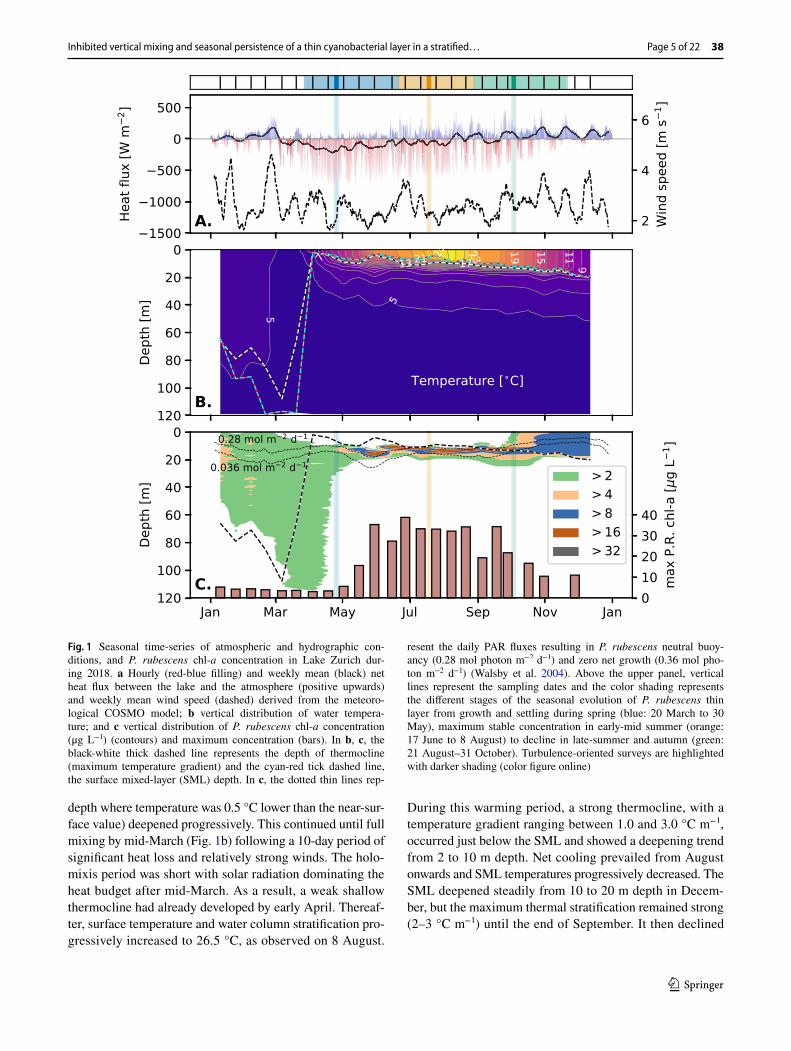
Figure 1 shows the evolution of atmospheric forcing and lake temperature at the monitoring station (st0) for Lake Zurich in 2018. From January to March, the lake lost heat to the atmosphere (Fig. 1a). The water column was weakly stratified in January and the surface mixed layer (SML, defined as the
Inhibited vertical mixing and seasonal persistence of a thin cyanobacterial layer in a stratified…
1 3
Page 5 of 22 38
depth where temperature was 0.5 °C lower than the near-sur-face value) deepened progressively. This continued until full mixing by mid-March (Fig. 1b) following a 10-day period of significant heat loss and relatively strong winds. The holo-mixis period was short with solar radiation dominating the heat budget after mid-March. As a result, a weak shallow thermocline had already developed by early April. Thereaf-ter, surface temperature and water column stratification pro-gressively increased to 26.5 °C, as observed on 8 August.
During this warming period, a strong thermocline, with a temperature gradient ranging between 1.0 and 3.0 °C m−1 , occurred just below the SML and showed a deepening trend from 2 to 10 m depth. Net cooling prevailed from August onwards and SML temperatures progressively decreased. The SML deepened steadily from 10 to 20 m depth in Decem-ber, but the maximum thermal stratification remained strong (2–3 °C m−1 ) until the end of September. It then declined
Fig. 1 Seasonal time-series of atmospheric and hydrographic con-ditions, and P. rubescens chl-a concentration in Lake Zurich dur-ing 2018. a Hourly (red-blue filling) and weekly mean (black) net heat flux between the lake and the atmosphere (positive upwards) and weekly mean wind speed (dashed) derived from the meteoro-logical COSMO model; b vertical distribution of water tempera-ture; and c vertical distribution of P. rubescens chl-a concentration (μg L−1 ) (contours) and maximum concentration (bars). In b, c, the black-white thick dashed line represents the depth of thermocline (maximum temperature gradient) and the cyan-red tick dashed line, the surface mixed-layer (SML) depth. In c, the dotted thin lines rep-
resent the daily PAR fluxes resulting in P. rubescens neutral buoy-ancy (0.28 mol photon m−2 d−1 ) and zero net growth (0.36 mol pho-ton m−2 d−1 ) (Walsby et al. 2004). Above the upper panel, vertical lines represent the sampling dates and the color shading represents the different stages of the seasonal evolution of P. rubescens thin layer from growth and settling during spring (blue: 20 March to 30 May), maximum stable concentration in early-mid summer (orange: 17 June to 8 August) to decline in late-summer and autumn (green: 21 August–31 October). Turbulence-oriented surveys are highlighted with darker shading (color figure online)
B. Fernández Castro et al.
1 3
38 Page 6 of 22
gradually as the SML expanded through the deeper part of the metalimnion, which was more weakly stratified.
Planktothrix rubescens was observed throughout the SML as relatively low chl-a concentrations (chl-a < 4 μg L−1 ) during the mixing period in winter and occurred throughout the water column after holomixis (Fig. 1c). From May onwards, P. rubescens communities formed a thin layer located within the main thermocline between 10 and 17 m depth. Planktothrix rubescens regu-late their vertical position according to the daily dosages of photosynthetically available radiation (PAR; Walsby et al. 2004). The records described here found P. rubescens mostly located between daily PAR isolines for which P. rube-scens acquires neutral buoyancy (0.28 mol photon m−2 d−1 ) and for which the net growth becomes zero (0.036 mol pho-ton m−2 d−1 ; thin dashed lines in Fig. 1c; Walsby et al. 2004). The layer remained stable, with peak concentrations between 30 and 40 μg L−1 , until October, when the thermo-cline deepened and approached the layer. From mid-October, P. rubescens concentration in the SML began to increase but the peak persisted until the end of the month, when the thermocline transgressed the layer, and the latter dispersed.
For the rest of the year, the P. rubescens population was located exclusively in the SML at moderate concentrations of ~ 10 μg L−1.
Microstructure measurements
Seasonal changes in stratification and mixing environment
Our turbulence sampling detected three stages in the seasonal development of the P. rubescens layer. The first microstruc-ture and HR-mooring survey was carried out between 24 and 26 April 2018 (blue, Fig. 1), shortly before formation of the thin layer. The second survey occurred between 17 and 19 July (orange), when the thin layer had been established for more than 2 months and water column stability approached its max-imum value. Finally, the third sampling took place between 2 and 4 October (green), when some P. rubescens chl-a had been detected in the SML but the chl-a peak remained sharp and well defined in spite of its reduced amplitude.
During the sampling in April, heating outpaced nighttime cooling and hourly wind speeds were maximal (6 m s−1 ) on the 25th, such that no microstructure profiles could be
Fig. 2 Hourly meteorological conditions (net heat flux, blue-red fill-ing; wind speed, dashed black) derived from the COSMO model dur-ing the 3 microstructure and mooring samplings in 2018: a 24–26 April 2018, b 17–19 July 2018, and c 2–4 October 2018. Median pro-files of d temperature, e buoyancy frequency and f chl-a fluorescence derived from the microstructure profiles at st1 for April 2018 (blue, SCAMP profiler), July 2018 (orange, VMP profiler) and October 2018 (green, VMP profiler). In a–c, microstructure profiles are indi-
cated with black ticks, and the duration of mooring deployments is indicated with color filling. In panels c–f the depth range of the P. rubescens thin layer, defined as the range where chl-a is larger than an e-folding fraction of the maximum value (chl-a > max (chl-a)/e, is indicated by filled rectangles for July (orange) and October (green). Individual profiles for chl-a are shown in f as semi-transparent lines. Individual profiles were projected onto isothermal coordinates to remove the effect of internal wave motions (color figure online)
Inhibited vertical mixing and seasonal persistence of a thin cyanobacterial layer in a stratified…
1 3
Page 7 of 22 38
carried out on that day. Except for this day, wind remained < 4 m s−1 (Fig. 2a). Thermal stratification was still moderate ( Nmax ≈ 0.02 s−1 ), with a shallow thermocline located above 5 m depth (Fig. 2d, e). Chl-a measured with the SCAMP was low ( < 5 μg L−1 ) and no thin layer was observed (Fig. 2f). In July, nighttime cooling intensified but daytime heat-ing still dominated the net heat budget. Maximum wind speeds of > 5 m s−1 were observed on the 19th (Fig. 2b). The water column was thermally stratified from the surface ( N ≈ 0.02 s−1 ), and a strong thermocline extended from 7 to 17 m depth with maximum stratification ( Nmax = 0.075 s−1 ) at 9 m depth (Fig. 2d, e). A ~2 m thick, vertically symmet-ric thin layer of chl-a (max. 30 μg L−1 ) occurred at 13 m, 4 m below the stratification maximum (Fig. 2f). In Octo-ber, nighttime cooling was prominent and daytime heating
had weakened. The relatively low wind speeds (2 m s−1 ), increased on 4 October (6 m s−1 , Fig. 2c). A homogeneous SML, not observed in the previous surveys, extended down to 10.5 m depth, and rested on an even sharper thermocline ( Nmax ≈ 0.1 s−1 at 11.5 m depth, Fig 2d, e). A weaker chl-a maximum (13 μg L−1 ) was observed at ~12 m depth coincid-ing with maximum N. The chl-a peak had broadened (4.5 m) to become asymmetric with a sharp upper edge (Fig. 2f).
April data gave elevated � values of 2 × 10⁻⁷ W kg−1 in the upper 8 m. Below this depth, � dropped sharply to very low values ( ≤ 10−10 W kg−1 ; Fig. 3a). In July and October, � showed a similar vertical distribution, with larger values between 4 × 10⁻⁹ and 4 × 10⁻⁸ W kg−1 in the upper 14 m, and a second maximum in the depth range of the main
Fig. 3 Mean profiles of turbulence-related variables derived from the microstructure profiles during 24–26 April 2018 (blue, SCAMP profiler), 17–19 July 2018 (orange, VMP profiler) and 2–4 October 2018 (green, VMP profiler) at st1. a TKE dissipation rate ( � ), b Thorpe ( LT , dotted lines) and Ozmidov ( LO , semi-transparent lines) length-scales, c buoyancy Reynolds number ( Reb ), and d turbulent heat diffusivity ( KT ). The 90% confidence intervals from bootstrap sampling are represented as faded horizontal lines. The depth range of the P. rubescens thin layer, defined as the range where chl-a is larger than an e-folding fraction of the maximum value (chl-a > max (chl-a)/e, is indicated by filled rectangles for July (orange) and October (green) (color figure online)
B. Fernández Castro et al.
1 3
38 Page 8 of 22
thermocline (10–13 m). From the base of the main thermo-cline, � decreased to 10−10 W kg−1 at 25 m depth.
The Thorpe scale, LT , describing the size of turbulent overturns, was 1–3 cm in the upper 10 m during April and gradually increased with depth to up to 10 cm at 20–25 m depth (Fig. 3b). In this deeper layer, LT was similar to the Ozmidov scale ( LO ), but LO was 10 times larger than LT in the upper 10 m. In July, LT , was ~3 cm in the upper 5 m but exhibited smaller thickness below ( LT = 1 mm to 1 cm). During this sampling, LO was also about one order of mag-nitude larger than LT throughout the water column. October data gave relatively large LT and LO values (10 cm to 1 m) that resembled each other in the upper 12 m. These declined sharply below 12 m to the order of ∼1 cm with LT being generally smaller than LO.
April data gave a buoyancy Reynolds number of Reb > 100 in the upper 8 m indicating energetic turbulence (Fig. 3c). At greater depths, Reb < 15 , except for a local peak at 12 m. Smaller values of Reb < 15 indicate that turbulence is buoyancy-suppressed (Ivey and Imberger 1991; Bouffard and Boegman 2013). In July, Reb exceeded 100 in the upper 5 m but declined rapidly below this depth to Reb < 15 in deeper layers. October data showed a sharp transition for Reb at 11 m depth from high values ( Reb ≈ 1000 ) in the SML to molecular values within the thermocline.
The turbulent heat diffusivity ( KT in Eq. 2) followed the same vertical distributions as those exhibited by Reb for the three sampling dates (Fig. 3d). KT approached (April) or fell below (July, October) molecular levels in the depth range where Reb ≲ 15 , including the metalimnion. April and July data gave
Fig. 4 Probability distribution of turbulence-related quantities within the P. rubescens layer, defined as the depth range where chl-a > max (chl-a)/e, derived from the microstructure profiles during 17–19 July 2018 (white bars) and 2–4 October 2018 (grey bars) at st1. a TKE dissipation rate ( � ), b Thorpe ( LT , bars) and Ozmidov ( LO , lines and filled patches) length-scales, c buoyancy Reynolds number ( Reb ), and d turbulent heat diffusivity ( KT ). Mean and median values are
represented by solid and dashed vertical lines, respectively (see val-ues in Table 1). Black lines are for July and grey lines for October, respectively. The probability of occurrence of molecular conditions according to the criteria Reb < 15 and KT ≤ �T is indicated in c, d, respectively. For the quantities depending on fitting to the theoreti-cal temperature-gradient spectrum ( � , Reb , LO , KT ), only good fits are shown (color figure online)
Inhibited vertical mixing and seasonal persistence of a thin cyanobacterial layer in a stratified…
1 3
Page 9 of 22 38
moderate KT values ( 10−5 m2 s−1 ) in the upper ~ 7 m, while October data gave large values (~10−2 m2 s−1 ) in the SML.
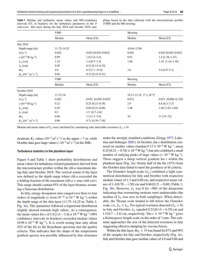
Turbulence statistics in the plankton layer
Figure 4 and Table 1 show probability distributions and mean values for turbulence-related parameters derived from the microstructure profiles within the chl-a maximum dur-ing July and October 2018. The vertical extent of the layer was defined as the depth range where chl-a exceeded the e-folding fraction of the maximum (chl-a > max (chl-a)/e). This range should contain 85% of the layer biomass assum-ing a Gaussian distribution.
In July, energy dissipation rates ranged over three to four orders of magnitude ( � from 10−10 to 10−6 W kg−1 ) within the depth range of the thin layer (11.75–14.25 m, Table 1; Fig. 4a). This parameter followed a lognormal distribution slightly skewed towards high values. As a consequence, the mean values for � of 1.8 [1.6 − 3.4] × 10−8 W kg−1 ( 90% confidence intervals in brackets) exceeded median values ( 0.99 × 10⁻⁸ W kg−1 ). It is worth noting that only about 42% of the fits to the Kraichnan spectrum met the quality criteria. This indicates that the shape of the temperature gradient spectra was possibly influenced by fine structures
under the strongly stratified conditions (Gregg 1977; Luke-tina and Imberger 2001). In October, the � distribution cen-tered on smaller values (median 0.12 × 10⁻⁸ W kg−1 , mean 0.25 [0.21 − 0.78] × 10−8 W kg−1 ) but also exhibited a small number of outlying peaks of large values ( > 10−8 W kg−1 ). These suggest a sharp vertical gradient for � within the plankton layer (Fig. 3a). Nearly half of the fits ( 47% ) from the October data failed to meet the goodness of fit criteria.
The Ozmidov length-scale ( LO ) exhibited a tight sym-metrical distribution for July and October with respective median values of 1.3 and 0.60 cm, and respective mean val-ues of 1.4 [0.70 − 1.50] cm and 0.66 [0.31 − 0.68] (Table 1; Fig. 4b). However, LT was 0 for ~90% of the datapoints indicating that overturning motions were undetectable (the median of LT was zero in both samplings). When detect-able, the Thorpe scale tended to fall below the Ozmidov scale, i.e., LT < LO . For typical overturns detected ( LT > 0 ) in July and October, LT equaled 0.23 [0.14 − 0.35] cm and 1.5 [0.7 − 2.8] cm, respectively. The � ≈ 10−8 W kg−1 gives a Kolmogorov length-scale on the order of 3 mm. This esti-mate approaches the size of the detected overturns in July suggesting effective damping by viscous forces.
Within the thin layer, Reb < 15 was found for 87% and 99% of the samples for July and October, respectively (Fig. 4c). July and October data gave median values of 4.8 and 0.86 and
Table 1 Median and arithmetic mean values and 90%-confidence intervals (CI, in brackets) for the turbulence parameters in the P. rubescens thin layer during the July 2018 and October 2018 sam-
plings based on the data collected with the microstructure profiler (VMP) and the HR-mooring
Median and mean values of LT were calculated by considering only detectable overturns ( L
T> 0)
VMP Mooring
Median Mean [CI] Median Mean [CI]
July 2018 Depth range [m] 11.75–14.25 10.84–12.90 N [s−1] 0.042 0.043 [0.025–0.043] 0.042 0.043 [0.042–0.043] � [10−8 W kg−1] 0.99 1.8 [1.6–3.4] 0.91 1.4 [1.38–1.47] L
O [cm] 1.25 1.4 [0.7–1.5] 1.08 1.18 [1.16–1.19]
LT [cm] 0.05 0.23 [0.14–0.35]
Reb
4.8 8.2 [7.1–14.9] 3.6 5.0 [4.9–5.1] K
T [ 10−7 m2 s−1] 0.04 0.12 [0.10–0.31]
VMP Mooring
Median Mean [CI] Median Mean [CI]
October 2018 Depth range [m] 11.75–16 10.13-12.19, T ≤ 18 °C N [s−1] 0.042 0.052 [0.050–0.055] 0.072 0.071 [0.068–0.139] � [10−8 W kg−1] 0.12 0.25 [0.21–0.78] 2.9 6.8 [6.3–7.3] L
O [cm] 0.59 0.66 [0.31–0.68] 1.46 1.66 [1.62–1.69]
LT [cm] 0.3 1.5 [0.7–2.8]
Reb
0.86 1.3 [1.2–2.8] 10 21 [19–23] K
T [ 10−7 m2 s−1] 0.06 0.71 [0.39–7.38]
B. Fernández Castro et al.
1 3
38 Page 10 of 22
mean values of 8.2 [7.1 − 14.9] , and 1.3 [1.2 − 2.8] indicating that non-turbulent, molecular fluxes prevailed. Estimated KT distributions for July (median: 0.04 × 10⁻⁷ m2 s−1 , mean: 0.12 [0.10 − 0.31] × 10−7 m2 s−1 ) and October (median: 0.06 × 10⁻⁷ m2 s−1 , mean: 0.71 [0.39 − 7.40] × 10−7 m2 s−1 ) agreed with the former estimates indicating that turbulent mixing did not enhance molecular heat fluxes.2
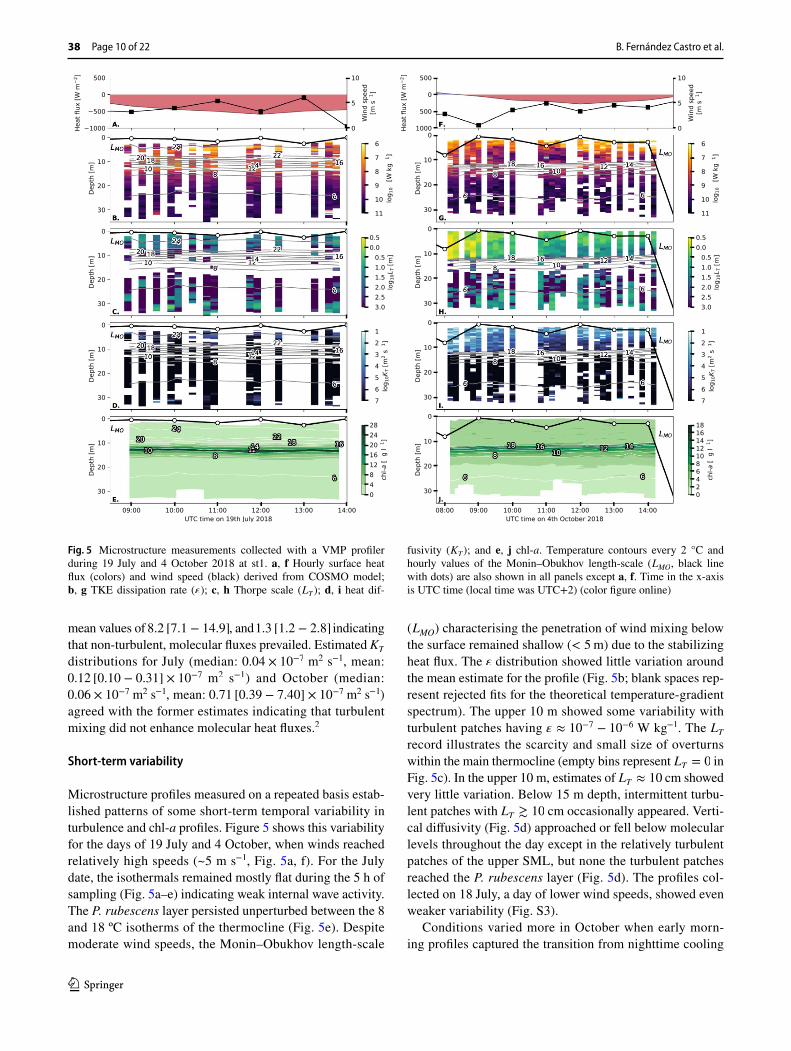
Short‑term variability
Microstructure profiles measured on a repeated basis estab-lished patterns of some short-term temporal variability in turbulence and chl-a profiles. Figure 5 shows this variability for the days of 19 July and 4 October, when winds reached relatively high speeds (~5 m s−1 , Fig. 5a, f). For the July date, the isothermals remained mostly flat during the 5 h of sampling (Fig. 5a–e) indicating weak internal wave activity. The P. rubescens layer persisted unperturbed between the 8 and 18 ºC isotherms of the thermocline (Fig. 5e). Despite moderate wind speeds, the Monin–Obukhov length-scale
( LMO ) characterising the penetration of wind mixing below the surface remained shallow ( < 5 m) due to the stabilizing heat flux. The � distribution showed little variation around the mean estimate for the profile (Fig. 5b; blank spaces rep-resent rejected fits for the theoretical temperature-gradient spectrum). The upper 10 m showed some variability with turbulent patches having � ≈ 10−7 − 10−6 W kg−1 . The LT record illustrates the scarcity and small size of overturns within the main thermocline (empty bins represent LT = 0 in Fig. 5c). In the upper 10 m, estimates of LT ≈ 10 cm showed very little variation. Below 15 m depth, intermittent turbu-lent patches with LT ≳ 10 cm occasionally appeared. Verti-cal diffusivity (Fig. 5d) approached or fell below molecular levels throughout the day except in the relatively turbulent patches of the upper SML, but none the turbulent patches reached the P. rubescens layer (Fig. 5d). The profiles col-lected on 18 July, a day of lower wind speeds, showed even weaker variability (Fig. S3).
Conditions varied more in October when early morn-ing profiles captured the transition from nighttime cooling
Fig. 5 Microstructure measurements collected with a VMP profiler during 19 July and 4 October 2018 at st1. a, f Hourly surface heat flux (colors) and wind speed (black) derived from COSMO model; b, g TKE dissipation rate ( � ); c, h Thorpe scale ( LT ); d, i heat dif-
fusivity ( KT ); and e, j chl-a. Temperature contours every 2 °C and hourly values of the Monin–Obukhov length-scale ( LMO , black line with dots) are also shown in all panels except a, f. Time in the x-axis is UTC time (local time was UTC+2) (color figure online)
Inhibited vertical mixing and seasonal persistence of a thin cyanobacterial layer in a stratified…
1 3
Page 11 of 22 38
to daytime heating and wind speeds increased during the morning (Fig. 5f). Over the 6 hours of sampling, the ther-mocline rose gradually by 2 m (Fig. 5g–j) indicating likely a basin-scale response to enhanced winds. The chl-a maximum appeared between the 8 and 18ºC isotherms and tracked a stable upwards movement (Fig. 5j). Esti-mates of turbulence remained relatively uniform between the upper part of the SML and the top of the P. rubescens layer until 9am. These indicated moderate levels of mixing with � ≈ 10−8 − 10−7 W kg−1 , KT ≈ 10−2 m2 s−1 and large turbulent overturns LT > 1 m (Fig. 5g–l). With the onset of warming, LMO diminished ( < 5 m), overturns decreased ( LT < 1 m) and � and KT declined, particularly in the lower part of the SML. As a result of the relatively strong winds, � and KT remained large in the upper SML down to 7–8 m depth. This daytime wind-driven sub-surface mixing how-ever did not reach the thermocline or cyanobacterial layer.
High‑resolution mooring observations within the thermocline
The high-resolution measurements by moored instruments revealed high-frequency internal wave variability not cap-tured by the profilers. The patterns detected included cm-scale vertical internal wave-driven isothermal displacements and velocities on cm s−1 scales (Fig. 6). In July, the sampling range (10.84–12.9 m depth) spanned a region included in the main thermocline with a relatively uniform and pronounced temperature gradient (roughly 3.5 °C over 2.5 m; Fig. 6a, b). The overall amplitude of fluctuations in current velocities and isothermal displacements varied little during the 8-h deployment. In October, the sampling range (10.13–12.19 m depth) included part of the SML at the beginning of the deployment. Measurements detected only the upper, sharper edge of the P. rubescens layer, located between the 18ºC and 15ºC isotherms (Fig. 6e, f). For the first two hours, back-ground currents were relatively weak with no fluctuations of the isotherms. After 10:30, current velocities increased gradually, and high-frequency fluctuations commenced. The intensification (up to a maximum of 5 cm s−1 at about 13:00)
Fig. 6 Measurements of horizontal eastward (u) and northward (v) velocities (filled contours in a, b, e, f), temperature (grey lines in all panels), inverse Richardson number ( 1∕Ri = S2∕N2 , c, g), and TKE dissipation rate ( � , d, h) obtained with the HR-mooring at st1 in July and October 2018. The position of the thermistors is indicated by horizontal dashed lines. Data on a–d were collected on 18 July 2018, and data on e–h correspond to 4 October 2018. The displayed
temperature and velocity signals were smoothed with a low-pass But-terworth filter with a 5-min period. Data in blank areas in d, h were excluded due to poor beam correlation (segment median correlation < 70% ). The isotherms corresponding to the mean location of chl-a maximum, and the upper and lower edges of the chl-a layer (e-folding fraction of the maximum value) are shown as green solid and dashed lines, respectively, in c, g (color figure online)
B. Fernández Castro et al.
1 3
38 Page 12 of 22
coincided with an expansion of the pycnocline such that it occupied the whole sampling range by the end of the deploy-ment. This event likely reflects rising winds that morning, which also appeared in the microstructure profiles.
Horizontal f low velocities documented ver ti-cal structure within a narrow, meter-scale range dur-ing both deployments. The shear in the mean f low ( S2 = (�u∕�z)2 + (�v∕�z)2 ) can trigger shear instabili-ties to drive turbulence and mixing if it overcomes the
Fig. 7 Microstructure measurements collected with a microCTD pro-filer during the nighttime sampling on 24–25 September 2019 at st0. a Hourly surface heat flux (colors) and wind speed (black) derived from COSMO model, b TKE dissipation rate ( � ), c Thorpe scale ( LT ), and d heat diffusivity ( KT ). Temperature contours every 2 °C and hourly values of the Monin–Obukhov length-scale ( LMO , black
line with dots) are plotted in b–d. Upward and downward looking triangles indicate ascending and descending profiling, respectively. The color scale of the triangles represents the sampling time. Surface mixing-layer depth (defined as LT > 1 m) is indicated with horizon-tal black markers in c. Time in the x-axis UTC time (local time was UTC+2) (color figure online)
Inhibited vertical mixing and seasonal persistence of a thin cyanobacterial layer in a stratified…
1 3
Page 13 of 22 38
stabilizing effect of stratification. This situation occurs when the gradient Richardson number ( Ri = N2
∕S2 ) falls below the critical value of 1/4 (Miles 1961). High-reso-lution measurements show that, despite the existence of background shear, unstable Ri were not often obtained, due to the strong stratification. Specifically, conditions in July and October met stable criteria ( Ri > 1 ) 88% and 80% of the time (Fig. 6c, g). Furthermore, most unstable val-ues occurred in October within the weakly-stratified SML. These exerted little effect on the thermocline, where the P. rubescens layer occurred.
Energy dissipation rates derived from turbulent veloc-ity fluctuations using structure functions ranged between 10−10 and 10−7 W kg−1 in July and rose to values on the order of 10−10 − 10−6 W kg−1 during October (Fig. 6d, h). In July, � exhibited intermittent structure between calmer (from 10:30 to 11:00 and between 12:00 and 13:00) and more dissipative conditions. The periods of lower dissipa-tion took place under conditions of reduced vertical shear when Ri < 1 events were not detected (Fig. 6c). In October, � began with weak values during the first 2 h, when inter-nal wave activity was weak and strengthened thereafter. The average � was 1.4 [1.4 − 1.5] × 10−8 W kg−1 (median: 0.91 × 10⁻⁸ ) and 6.8 [6.3 − 7.3] × 10−8 W kg−1 (median: 2.9 × 10⁻⁸ ) for July and October, respectively. Table 1 lists these values as well as their respective ranges. The values in July showed very good agreement with microstruc-ture estimates for the same depth range (Fig. 3a). Values derived for LO and Reb also resembled those derived form profile observations (Table 1). In October, high-resolu-tion velocities gave somewhat larger values for � , but, Reb remained in the range indicating a molecular regime (mean 21 [19 − 23] , median: 10).
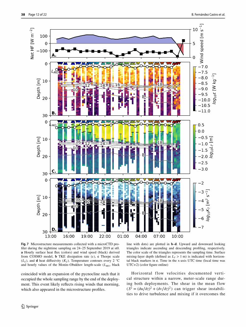
Nighttime sampling: the role of convective mixing
The asymmetric vertical distribution of chl-a in October and enhanced turbulence during the early morning of 4 October 2018 (before solar heating outpaced heat lost) suggest that convective mixing in autumn could potentially disrupt the P. rubescens layer and cause the decline observed in the long-term data (Fig. 1). It was not possible to test this idea with the 2018 dataset, since daytime measurements do not capture layer dynamics during fully developed convective mixing.
To overcome this limitation, a nighttime survey was conducted with a microstructure profiler, a CTD and a FluoroProbe between 14:40 UTC (16:40 local) on 24 Sep-tember 2019 and 10:40 on 25 September 2019 (Fig. 7). This field campaign occurred under conditions of low wind speeds (2 m s−1 ) and moderate heat loss (Fig. 7a). Observations recorded a 10 m SML with T = 18 °C and a sharp pycnocline between 10 and 15 m depth (Fig. 7b). Consistent with the previous results, data failed to pro-vide good fits to the theoretical temperature-gradient spectrum for the thermocline. As a consequence, � could not be determined in several instances (Fig. 7b). Turbu-lent overturns were rare (Fig. 7c), and vertical diffusiv-ity approached or fell below molecular values (Fig. 7d). The SML, below the Monin-Obukhov depth gave initially low values for � ( 10−10 W kg−1 ) with LT < 1 m and KT approaching molecular scale. After 17:00, a mixing layer with enhanced � ( 2 × 10⁻⁸ W kg−1 ), LT ( > 1 m) and KT ( > 10−4 m2 s−1 ) penetrated beneath LMO . At about 21:00, the mixing reached the thermocline, which also deepened slightly overnight. The intensity and downward penetra-tion of the convective mixing declined after 04:00 and completely ceased after sunrise when the heat flux was negative (into the lake).
Fig. 8 Profiles of P. rubescens chl-a concentration collected dur-ing the nighttime sampling on 24–25 September 2019 at st0 with a FluoroProbe. The profile at the indicated sampling time (color rectan-gle) is shown as a black line, and initial reference profile collected at
14:40 is shown as a light blue line. The bars represent mean profiles of Thorpe scale ( LT ) between the previous and current FluoroProbe profile. The color code indicates the sampling time in relation to Fig. 7 (color figure online)
B. Fernández Castro et al.
1 3
38 Page 14 of 22
Figure 8 shows effects of convective mixing on P. rubescens distribution as determined by the FluoroProbe measurements. The initial profiles in the early afternoon (14:40) are plotted in light blue in every panel for clar-ity, and bars representing the LT are included to illustrate the vertical extent and intensity of mixing. Planktothrix rubescens appears as a well defined peak in the after-noon and at relatively low concentration in the SML. Overnight, convection reached the top of the thin layer. The maximum P. rubescens layer concentration progres-sively declined and the community’s concentration in the SML increased due to filament entrainment by convec-tive plumes eroding the layer from above. These results clearly show the disruptive effect of nighttime convection on the structure of the P. rubescens metalimnetic layer in early autumn.
Discussion
On the nature of suppressed thermocline mixing
Independent estimates of TKE dissipation with microstruc-ture and high-resolution current measurements in the highly stratified seasonal thermocline of Lake Zurich revealed mod-erate levels of dissipation, � ≈ 10−8 W kg−1 . Dissipation exhibited a degree of intermittency spanning three orders of magnitude. The turbulent heat diffusivity, KT , exhibited persistently small values of the order of 10−8 m2 s−1 . Their scale relative to the molecular heat diffusivity means that turbulent fluxes across the thermocline were negligible. These estimates indicate very limited mixing efficiency ( � = KTN
2∕� ≈ 0.002 ) wherein most of the TKE is lost
to viscous dissipation and does not produce mixing. Data also revealed infrequent unstable Richardson number values ( Ri < 1∕4 ) and vertical turbulent overturns ( ≲ 10% occur-rence) within detection limits. Detected overturns were characterised by LT ≤ LO ≈ 2 cm, which fell below typical values in the ocean thermocline (Gregg 1987) and even the lowest estimates from hypolimnetic observations in lakes (Etemad-Shahidi and Imberger 2001; Lorke and Wüest 2002). Vertical turbulent overturns store available potential energy, 0.5L2
TN2 (Dillon and Park 1987), which is transferred
to the mean density profile when overturns collapse. The scarcity of overturns and their small size thus provide strong indication of very weak turbulent mixing in the thermocline.
Different sources of evidence, including observations, laboratory experiments and simulations, indicate that tur-bulent fluxes become negligible when the buoyancy Reyn-olds number ( Reb = (LO∕LK)
4∕3 ), which measures of the size of the inertial subrange ( LO > l > LK ), falls below O(10 − 100) (Ivey and Imberger 1991; Gibson 1999; Shih et al. 2005). Our thermocline observations fall mostly
within this range and thus explain the relative weak mix-ing observed. Another parameter used to estimate mix-ing efficiency of turbulence is the turbulent Froude num-ber, FrT = (LO∕LT )
2∕3 . This parameter represents a ratio between the turbulent eddy size required to achieve an equilibrium between inertial and buoyancy forces ( LO ) and the observed vertical eddy size ( LT ). When FrT approaches or falls below one, turbulent eddies begin to disrupt back-ground stratification, and the system experiences its maximum potential for turbulent mixing (Mashayek et al. 2017). Because LT values fell far below LO for our dataset on the Lake Zurich thermocline, FrT was very large. This means that the turbulent eddies were too small to disturb the background stratification. Instead, low mean values for Reb and LT (the latter sometimes close to the Kolmogorov scale) suggest strong dampening of turbulent motions by viscosity (Ivey and Imberger 1991). Such situations can produce only very weak turbulent fluxes, consistent with those appearing in the observations described here.
Overall, the results presented here comport with previous turbulence measurements in small and medium size lakes, which showed only very weak turbulent fluxes occurring in their interiors (Saggio and Imberger 2001; Etemad-Sha-hidi and Imberger 2001; Boegman et al. 2003; MacIntyre et al. 2009; Weck and Lorke 2017). Mixing at the basin-scale depends most strongly on processes occurring at the boundaries (Goudsmit et al. 1997; Wüest et al. 2000; Mac-Intyre et al. 1999). With direct measurements using eddy covariance, Etemad-Shahidi and Imberger (2001) and Sag-gio and Imberger (2001) quantified turbulent fluxes in the thermoclines of two stratified lakes. These researchers found similar situations to that described here for Lake Zurich, wherein high dissipation rates ( � ≈ 10−7 W kg−1 ) occurred only with small scale overturns and negligible vertical fluxes. The authors interpreted turbulent dissipation as driven by wave–wave interactions, which resulted in high-intermittency and weak vertical fluxes rather than formation of overturning billows due to shear instabilities (Itsweire et al. 1993; Teoh et al. 1997). Turbulence properties of the Lake Zurich metalimnion also resembled those reported in association with thin plankton layers in the ocean. These layers are frequently found within sharp thermoclines, where Reb (McManus et al. 2003; Broullón et al. 2020) and vertical diffusivities (Steinbuck et al. 2009) are small ( Reb < 100 and KT ≲ 10−6 m2 s−1 ) suggesting weak vertical turbulent mixing.
Turbulence characterised by low Reb and only occa-sional small scale overturns, suggests anisotropic turbulent motions. These conditions violate assumptions underlying methodologies used to calculate � both from microstructure and high-resolution current measurements (Dillon and Cald-well 1980; Smyth and Moum 2000; Bluteau et al. 2011) such that the large � values must be interpreted with caution.
Inhibited vertical mixing and seasonal persistence of a thin cyanobacterial layer in a stratified…
1 3
Page 15 of 22 38
About half of the temperature-gradient spectral fits were dis-carded because the observational spectra did not follow the expected shape according to the established fit criteria. This indicates that conditions were possibly not turbulent in all cases, and fine-scale structures influenced the spectra (Gregg 1977). Dissipation rates derived from high-resolution veloci-ties also depend on a multiplicative fit constant. Under uni-sotropic conditions, this could deviate from the prescribed isotropic value and generate uncertainties of > 50% in the estimates (Jabbari et al. 2016). Agreement between the two different methods and the consistency with previous obser-vations allow for a certain degree of confidence in our results however. Substantial errors associated with � estimates fur-thermore would not compromise first order interpretations of suppressed metalimnetic mixing.
Basin‑scale mixing and thin layer persistence
In addition to its well known seasonal persistence, our high-resolution measurements revealed the exceptional stability of the P. rubescens thin layer at sub-daily scales (Fig. 5). This only abated when nighttime convective mixing pen-etrated into the layer during the September 2019 sampling. The persistence appears due to the reduced turbulent fluxes in the metalimnion. However, our sampling strategy may have undersampled the effect of turbulent mixing on the P.
rubescens thin layer for two reasons. First, the forcing con-ditions during the four surveys may not have captured the full range of weather variability. Second, the P. rubescens community occurs throughout the lake (Salcher et al. 2011; Garneau et al. 2015) including along slope and near-shore regions. As such, the likely effects of boundary mixing (Goudsmit et al. 1997) on the community would not appear in offshore observations like the ones conducted here.
To investigate the role of unresolved mixing, we used hourly meteorological data and bi-weekly water column observations to calculate the lake number ( LN ). We also estimated a basin-scale turbulent diffusivity using the heat budget method and a surface boundary layer scaling (see Supplementary Text 1 for details) (Fig. 9). The lake number indicates the potential of wind stress to significantly disturb the metalimnion by driving upwelling and exciting inter-nal motions. Significant disturbance occurs when LN < 10 . LN exhibited values <10 almost every day over the winter period until April (Fig. 9b). This indicates that wind forc-ing could easily overcome the existing weak stratification and drive turbulent mixing. From April, the number of days when LN < 10 progressively declines such that no such days occurred in June and throughout the entire summer. This indicates strong damping of interior motions and mixing by stratification. Mixing events reappeared from October onward as the deepening of the SML progressively eroded
Fig. 9 a Basin-scale vertical heat diffusivity ( KBST
; derived from the heat budget method in the meta- and hypolimnetic layers, and from a boundary layer scaling in the SML) for the spring (blue: 20 March–30 May), mid-summer (orange: 17 June–8 August) and late-summer/autumn (green: 21 August–31 October) periods; b time-series of hourly (grey) and weekly (black) lake number ( LN ) and cumula-tive counts of days when LN < 10 during at least one hour (red);
and c weekly counts of convectively stable ( LMO < 0 ) and unsta-ble ( LMO > 0 ) situations when the absolute value of LMO is smaller/larger than the depth of the surface mixed-layer ( zSML ). Dark-red and dark-blue filling indicate conditions favorable for wind-driven entrainment in the metalimnion ( |LMO| > zSML ). Counts of situations when strong winds (twice the median value) could cause entrainment ( |LMO| > zSML ) are shown as a thin back line. The mean SML depths are shown as circles in a (color figure online)
B. Fernández Castro et al.
1 3
38 Page 16 of 22
stratification. The high summer LN values indicate that inter-nal wave dynamics in the lake generally follow the linear regime described by Horn et al. (2001) of reduced energy transfer to small scales and reduced mixing. This confirms the interpretation that our microstructure surveys accurately represent summer conditions in Lake Zurich.
Consistent with the seasonal evolution of LN , spring time measurements gave higher mean basin-scale vertical heat diffusivity ( KBS
T , Fig. 9a) below the SML (~1 ×10⁻⁵ m2 s−1 )
than that estimated for summer and autumn periods ( 10−6 − 10−5 m2 s−1 ). Mixing was suppressed at ~ 12 m depth ( ~15 m) during summer and fall. Data from these times gave KBST
values as low as 1 − 2 × 10⁻⁶ m2 s−1 . Despite large LN values during summer months, the metalimnetic basin-scale diffusivity exceeded molecular scales by an order of magni-tude. This indicates weak but detectable mixing.
To understand how P. rubescens filaments navigate mix-ing to maintain their vertical position, we compared the ver-tical restoring velocities that the P. rubescens filaments can achieve when displaced from their depth of neutral buoyancy ( wbuoy ), with the velocities required to compensate for dis-persion by turbulent mixing ( weq ) (Fig. 10). This required an equilibrium velocity that was calculated by integrating the advection-diffusion equation assuming steady state and zero net growth (Stacey et al. 2007; Steinbuck et al. 2009):
where C represents the concentration profile. In this case we used the P. rubescens chl-a profiles from the bi-weekly moni-toring at the beginning of each period (Fig. 1). Figure 9 shows vertical diffusivity profiles used as KBS
T . The restoring velocity
represents the balance between buoyancy and drag forces:
where rs is the equivalent spherical radius of a filament ( ∼ 2 � m; Walsby 2005), �fill is the density of the filaments, and � ≈ 3.97 is a form factor for cylindrical filaments. We assumed that for short term perturbations, the density of the filaments equals the density of water at the P. rubescens chl-a peak. However, laboratory cultures have shown that if the filaments are exposed to higher (lower) light levels for suf-ficiently long periods of several hours or days, they gain ballast (buoyancy) to a maximum (minimum) anomaly of �fil − � = +27 kg m−3 (-30 kg m−3 ). In this situation, the restoring velocities would reach maximum values according to Eq. (6) ( wmax
buoy≈ 0.58 m d−1 ; Walsby 2005). Here, we will
refer to the latter as a long-term response.
(5)weq(z) = KBST(z)
�
�z
[ln
(C(z)
Cmax
)],
(6)wbuoy(z) =2gr2
s(1 − �fil∕�(z))
9��,
Fig. 10 Vertical velocity ( weq , triangles) required for P. rubescens to outcompete turbulent diffusion, as derived from the advection-dif-fusion balance (Eq. 5). Upward (downward) velocities are shown as filled upward-pointing (empty downward-pointing) triangles. Stokes velocities ( wbuoy ) for P. rubescens filaments having their neu-tral density at the P. rubescens peak are shown as black solid lines (i.e. short-term response). Maximum P. rubescens stokes velocities
(i.e. long-term response) for maximum/minimum density anoma-lies (+27 / −30 kg m−3 ) observed for P. rubescens in lab cultures are shown as dashed lines, positive (resp. negative) anomalies are used above (resp. below) the peak. The P. rubescens chl-a profile at the beginning of each period is shown in grey. Spring, summer and autumn periods are as defined in Fig. 1
Inhibited vertical mixing and seasonal persistence of a thin cyanobacterial layer in a stratified…
1 3
Page 17 of 22 38
For all the periods, the short-term restoring velocities ( wbuoy < 0.1 m d−1 ) fell below the equilibrium velocities (Fig. 10), suggesting that episodic mixing events disrupt the layer on a transient basis. This situation changes when con-sidering the long-term response ( wmax
buoy ) indicating that the
buoyancy regulation capacity can generally restore the layer after mixing events. In spring, when P. rubescens lived below 10 m depth without layer formation, equilibrium velocities of 0.1–0.5 m d−1 approached but generally fell below restoring velocities (Fig. 10a). This indicates favora-ble conditions for the P. rubescens motility in rising from deeper zones to form the layer. The time-scale for layer for-mation by buoyancy alone would equate to � ≈ (|zmean|∕2)∕wmax
buoy≈ 44 days. This estimate shows good
agreement with observations since stratification began at the end of March and the plankton layer was first observed in early May. Vertical migration thus appears to initiate the layer.
In summer and autumn, equilibrium velocities ( weq ≈ 0.1 m d−1 ) below the layer were several times smaller than wmax
buoy . This explains the stability of the layer. Equilib-
rium velocities increased towards the upper edge of the layer in both periods but remained weq ≲ wmax
buoy during summer. In
autumn weq > wmaxbuoy
, which is consistent with entrainment of the layer by sub-surface mixing.
The role of convective mixing vs. wind mixing
This analysis corroborates direct observations and suggests that metalimnetic mixing driven by internal motions in the interior of the basin or at its boundaries, does not generally reach strengths necessary to overcome P. rubescens mobil-ity. Penetration of sub-surface mixing can disrupt the layer from above in autumn when the SML deepens across the metalimnion. Microstructure observations also suggest that, at least at the time of sampling, direct SML wind-driven mixing does not penetrate deep enough to produce entrain-ment of the P. rubescens layer. Nighttime convective mix-ing however generates overturns large enough to penetrate depths necessary to disrupt the P. rubescens layer in autumn. This suggests that convective mixing is responsible for the layer breakdown in autumn.
To assess the generality of this conclusion, we quanti-fied the frequency of conditions favorable for wind and convective entrainment at the base of the SML by compar-ing the Monin–Obukhov length ( LMO ) and the SML depth ( zSML ) (Fig. 9c). When LMO < 0 , the lake is warming (stable conditions). The reverse applies for lake cooling (unstable conditions). Wind can potentially produce entrainment in the metalimnion when |LMO| > zSML under either stable or unstable conditions. Fig. 9c shows that conditions for
wind-driven entrainment occurred frequently only in late spring (April–June), when the SML was shallow. The fre-quency of wind-driven entrainment peaked at ∼80% in early April. Strong wind events occurred with 20–30% frequency (see figure caption). From June to December |LMO| > zSML events were rare ( 10% frequency). Over that period, unstable conditions potentially conducive to convective entrainment of the thermocline become more and more prevalent ( 50% in July to 80% in December). These results indicate that the deepening of the SML in late summer and autumn occurs due to convective mixing and not wind mixing. In summer, the P. rubescens layer is located at the core of the metalim-nion, ∼5 m below the base of the SML. Entrainment cannot disturb it at this position. Once the SML reaches the top of the P. rubescens layer in autumn, however, nighttime con-vective mixing can entrain the layer and cause its seasonal breakdown.
Comparison with Lake Geneva
Planktothrix rubescens is a widespread species found throughout the world, particularly in perialpine lakes. For those lakes in which P. rubescens accumulates as a met-alimnetic thin layer in summer, these bacteria become the dominant planktonic species for several years or decades. Lakes Zurich, Hallwil (Stöckli 2012) and Baldegg (Buergi and Stadelmann 2000) in Switzerland, and Lac de Bourget in France (Jacquet et al. 2005) show this trend. However, in Lake Geneva (Switzerland/France), P. rubescens occurs only in modest concentrations and mainly during autumn months (CIPEL 2019). Furthermore, P. rubescens popula-tions have declined or disappeared in some lakes (i.e., Lac de Bourget, Jacquet et al. 2014), while they remain abundant in others that possess apparently similar nutrient regimes (i.e., Lake Zurich, Posch et al. 2012). To elucidate the reasons behind these differences, Jacquet et al. (2005) analysed a series of bio-physical parameters from two lakes with similar environmental conditions, including a recent history of re-oligotrophication, but also having strongly divergent concen-trations of P. rubescens (Lac de Bourget and Lake Geneva). These researchers interpreted higher water column stability as contributing to the abundant P. rubescens observed in Lac de Bourget.
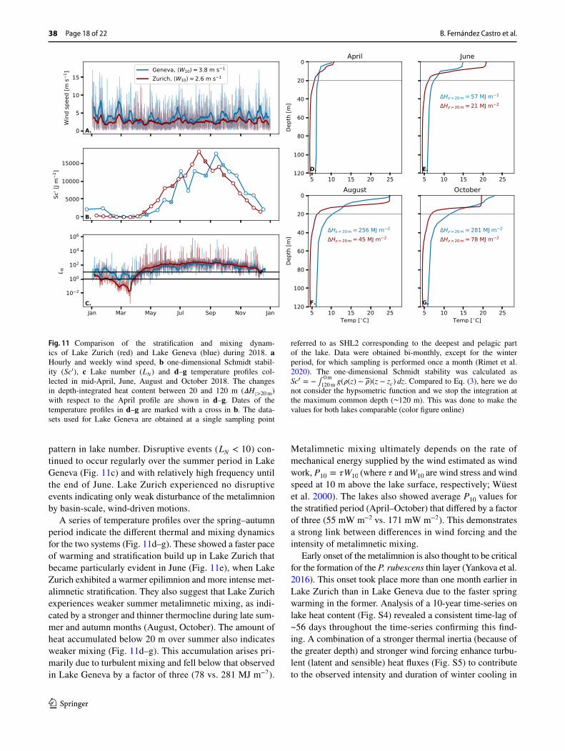
Here, we extended this comparison between Lake Geneva and Lake Zurich using meteorological and hydrographic data collected in 2018. Wind speeds were generally weaker over Lake Zurich (2.6 m s−1 ) relative to those affecting Lake Geneva (3.8 m s−1 ) (Fig. 11a). Bulk water column stability, calculated as the one-dimensional version of the Schmidt stability ( Sc′ , see caption of Fig. 11) exhibited similar maxi-mum summer values but estimates for Lake Geneva showed a delay of more than one month with respect to Lake Zurich (Fig. 11b). These two parameters conferred a different
B. Fernández Castro et al.
1 3
38 Page 18 of 22
pattern in lake number. Disruptive events ( LN < 10 ) con-tinued to occur regularly over the summer period in Lake Geneva (Fig. 11c) and with relatively high frequency until the end of June. Lake Zurich experienced no disruptive events indicating only weak disturbance of the metalimnion by basin-scale, wind-driven motions.
A series of temperature profiles over the spring–autumn period indicate the different thermal and mixing dynamics for the two systems (Fig. 11d–g). These showed a faster pace of warming and stratification build up in Lake Zurich that became particularly evident in June (Fig. 11e), when Lake Zurich exhibited a warmer epilimnion and more intense met-alimnetic stratification. They also suggest that Lake Zurich experiences weaker summer metalimnetic mixing, as indi-cated by a stronger and thinner thermocline during late sum-mer and autumn months (August, October). The amount of heat accumulated below 20 m over summer also indicates weaker mixing (Fig. 11d–g). This accumulation arises pri-marily due to turbulent mixing and fell below that observed in Lake Geneva by a factor of three (78 vs. 281 MJ m−2 ).
Metalimnetic mixing ultimately depends on the rate of mechanical energy supplied by the wind estimated as wind work, P10 = �W10 (where � and W10 are wind stress and wind speed at 10 m above the lake surface, respectively; Wüest et al. 2000). The lakes also showed average P10 values for the stratified period (April–October) that differed by a factor of three (55 mW m−2 vs. 171 mW m−2 ). This demonstrates a strong link between differences in wind forcing and the intensity of metalimnetic mixing.
Early onset of the metalimnion is also thought to be critical for the formation of the P. rubescens thin layer (Yankova et al. 2016). This onset took place more than one month earlier in Lake Zurich than in Lake Geneva due to the faster spring warming in the former. Analysis of a 10-year time-series on lake heat content (Fig. S4) revealed a consistent time-lag of ~56 days throughout the time-series confirming this find-ing. A combination of a stronger thermal inertia (because of the greater depth) and stronger wind forcing enhance turbu-lent (latent and sensible) heat fluxes (Fig. S5) to contribute to the observed intensity and duration of winter cooling in
Fig. 11 Comparison of the stratification and mixing dynam-ics of Lake Zurich (red) and Lake Geneva (blue) during 2018. a Hourly and weekly wind speed, b one-dimensional Schmidt stabil-ity ( Sc′ ), c Lake number ( LN ) and d–g temperature profiles col-lected in mid-April, June, August and October 2018. The changes in depth-integrated heat content between 20 and 120 m ( 𝛥Hz>20m ) with respect to the April profile are shown in d–g. Dates of the temperature profiles in d–g are marked with a cross in b. The data-sets used for Lake Geneva are obtained at a single sampling point
referred to as SHL2 corresponding to the deepest and pelagic part of the lake. Data were obtained bi-monthly, except for the winter period, for which sampling is performed once a month (Rimet et al. 2020). The one-dimensional Schmidt stability was calculated as Sc� = − ∫ 0m
120mg(�(z) − �)(z − zc) dz . Compared to Eq. (3), here we do
not consider the hypsometric function and we stop the integration at the maximum common depth ( ∼120 m). This was done to make the values for both lakes comparable (color figure online)
Inhibited vertical mixing and seasonal persistence of a thin cyanobacterial layer in a stratified…
1 3
Page 19 of 22 38
Lake Geneva. Lake size and the intensity of wind forcing thus appear to be factors supporting P. rubescens growth and development. P. rubescens thrives in mid-sized lakes deep enough to sufficiently isolate the metalimnion from surface and bottom enhanced turbulence, but shallow enough so that thermal inertia allows for an early onset of stratification. Mean and maximum depths of lakes Hallwil, Baldegg, Bourget and Zurich fall in intermediate ranges of 28–45 m and 48–145 m, respectively, relative to Lake Geneva which has mean and maximum depths of 155 m and 309 m, respectively.
Conclusions
This study investigated the interaction between vertical mixing and the seasonal persistence (May–October) of an annually recurring thin layer of toxic cyanobacteria (P. rubescens) in Lake Zurich using four microstructure surveys and high-resolution mooring deployments. Our measurements revealed that strong metalimnetic stratifi-cation inhibits overturning motions and vertical turbulent fluxes which provides a very stable environment for the P. rubescens thin layer to form and persist. Comparable sets of measurements available from the oceanographic literature describe similar turbulent environments for a variety of thin plankton layers which frequently appear in association with strong pycnoclines and weakly turbulent or laminar conditions. However, while oceanic features are ephemeral due to frequent disruption by episodic turbu-lence, weak mixing conditions can persist in Lake Zurich during summer. Our analysis showed that neither entrain-ment due to surface wind-driven turbulence nor metal-imnetic mixing, related to the dissipation of internal lake motions reach the strengths or frequencies necessary to disrupt the layer. This explains its extraordinary seasonal persistence. Instead, the layer breakdown in autumn occurs due to convective deepening of the surface mixed-layer.
A comparative analysis of Lake Geneva, which does not host a P. rubescens layer, indicates that low wind forcing (underpinning the weak metalimnetic mixing) and an early onset of stratification (allowed by weak thermal inertia com-pared to larger lakes) favor the proliferation and stability of P. rubescens in the form of a thin layer. These two facts would explain why P. rubescens can form thin layers and thrive in medium-sized lakes. Persistent and thin metalimnetic chloro-phyll maxima and weak interior turbulent mixing are common features in many lakes. Our results illustrate their connections and underline the relevance of convective mixing in the sea-sonal evolution of plankton blooms in stratified waters.
Supplementary Information The online version contains supplemen-tary material available at https:// doi. org/ 10. 1007/ s00027- 021- 00785-9.
Acknowledgements We acknowledge Sébastien Lavanchy (EPFL) and Michael Plüss (Eawag) for their contribution to the design of the HR-mooring and participation in the field campaigns. We thank Eugen Loher and Daniel Marty for their contribution to the bi-weekly moni-toring program. We are grateful to Tomy Doda, Lucas Serra Moncadas, Adem Topak, Camille Minaudo and Luca Cortese for their assistance during fieldwork and MeteoSwiss for the COSMO-1 weather data. This work was financed by the Swiss National Science Foundation Sinergia grant CRSII2_160726 (A Flexible Underwater Distributed Robotic Sys-tem for High-Resolution Sensing of Aquatic Ecosystems), and Grant 200021_179123 (Primary Production Under Oligotrophication in Lakes). This study was also supported by the grant SeeWandel: Life in Lake Constance - the past, present and future within the framework of the Interreg V-Program Alpenrhein–Bodensee–Hochrhein (Germany, Austria, Switzerland, Liechtenstein) which funds are provided by the European Regional Development Fund as well as the Swiss Confedera-tion and Cantons. The funders had no role in study design, data collec-tion and analysis, decision to publish, or preparation of the manuscript.
Funding Open Access funding provided by EPFL Lausanne.
Compliance with ethical standards
Conflict of interest The authors declare no conflict of interest.
Open Access This article is licensed under a Creative Commons Attri-bution 4.0 International License, which permits use, sharing, adapta-tion, distribution and reproduction in any medium or format, as long as you give appropriate credit to the original author(s) and the source, provide a link to the Creative Commons licence, and indicate if changes were made. The images or other third party material in this article are included in the article’s Creative Commons licence, unless indicated otherwise in a credit line to the material. If material is not included in the article’s Creative Commons licence and your intended use is not permitted by statutory regulation or exceeds the permitted use, you will need to obtain permission directly from the copyright holder. To view a copy of this licence, visit http:// creat iveco mmons. org/ licen ses/ by/4. 0/.
References
Abbott MR, Denman KL, Powell TM, Richerson PJ, Richards RC, Goldman CR (1984) Mixing and the dynamics of the deep chloro-phyll maximum in Lake Tahoe. Limnol Oceanogr 29(4):862–878. https:// doi. org/ 10. 4319/ lo. 1984. 29.4. 0862
Baracchini T, Bärenzung K, Bouffard D, Wüest A (2019) Le Lac de Zurich en ligne - Prévisions hydrodynamiques 3D en temps-réel sur meteolakes.ch. Aqua Gas - Fachzeitschrift für Gas, Wasser und Abwasser 99(12):24–29
Benoit-Bird KJ, Cowles TJ, Wingard CE (2009) Edge gradients pro-vide evidence of ecological interactions in planktonic thin layers. Limnol Oceanogr 54(4):1382–1392. https:// doi. org/ 10. 4319/ lo. 2009. 54.4. 1382
Bluteau CE, Jones NL, Ivey GN (2011) Estimating turbulent kinetic energy dissipation using the inertial subrange method in environ-mental flows. Limnol Oceanogr Methods 9:302–321. https:// doi. org/ 10. 4319/ lom. 2011.9. 302
Bouffard D, Boegman L (2013) A diapycnal diffusivity model for strati-fied environmental flows. Dyn Atmos Ocean 61–62:14–34. https:// doi. org/ 10. 1016/j. dynat moce. 2013. 02. 002
Broullón E, López-Mozos M, Reguera B, Chouciño P, Doval MD, Fernández-Castro B, Gilcoto M, Nogueira E, Souto C, Mouriño-Carballido B (2020) Thin layers of phytoplankton and harm-ful algae events in a coastal upwelling system. Prog Oceanogr 189:102449. https:// doi. org/ 10. 1016/j. pocean. 2020. 102449
Buergi HR, Stadelmann R (2000) Change of phytoplankton diversity during long-term restoration of Lake Baldegg (Switzerland). Verh Internat Verein Limnol 27(1):574–581. https:// doi. org/ 10. 1080/ 03680 770. 1998. 11901 300
Cheriton OM, McManus MA, Stacey MT, Steinbuck JV (2009) Physi-cal and biological controls on the maintenance and dissipation of a thin phytoplankton layer. Mar Ecol Prog Ser 378:55–69. https:// doi. org/ 10. 3354/ meps0 7847
CIPEL (2019) Rapports sur les études et recherches entreprises dans le bassin Lémanique. Tech. rep., Conseil Scientifique de la Commi-sion Internationale pour la Protection des Eaux du Léman, Thonon les Bains. ISSN 1010-8432
Dekshenieks MM, Donaghay PL, Sullivan JM, Rines JE, Osborn TR, Twardowski MS (2001) Temporal and spatial occurrence of thin phytoplankton layers in relation to physical processes. Mar Ecol Prog Ser 223:61–71. https:// doi. org/ 10. 3354/ meps2 23061
Dillon TM, Caldwell DR (1980) The Batchelor spectrum and dissipa-tion in the upper ocean. J Geophys Res 85(C4):1910–1916. https:// doi. org/ 10. 1029/ JC085 iC04p 01910
Dillon TM, Park MM (1987) The available potential energy of over-turns as an indicator of mixing in the seasonal thermocline. J Geophys Res 92(C5):5345–5353. https:// doi. org/ 10. 1029/ JC092 iC05p 05345
Durham WM, Stocker R (2012) Thin phytoplankton layers: characteris-tics, mechanisms, and consequences. Ann Rev Mar Sci 4(1):177–207. https:// doi. org/ 10. 1146/ annur ev- marine- 120710- 100957
Ernst B, Hoeger SJ, O’Brien E, Dietrich DR (2009) Abundance and toxicity of Planktothrix rubescens in the pre-alpine Lake Ammer-see, Germany. Harmful Algae 8(2):329–342. https:// doi. org/ 10. 1016/j. hal. 2008. 07. 006
Etemad-Shahidi A, Imberger J (2001) Anatomy of turbulence in ther-mally stratified lakes. Limnol Oceanogr 46(5):1158–1170. https:// doi. org/ 10. 4319/ lo. 2001. 46.5. 1158
Fink G, Schmid M, Wahl B, Wolf T, Wüest A (2014) Heat flux modi-fications related to climate-induced warming of large European lakes. Water Resour Res 50:2072–2085. https:// doi. org/ 10. 1002/ 2013W R0144 48
Garneau MÈ, Posch T, Pernthaler J (2015) Seasonal patterns of micro-cystin-producing and non-producing Planktothrix rubescens geno-types in a deep pre-alpine lake. Harmful Algae 50:21–31. https:// doi. org/ 10. 1016/j. hal. 2015. 10. 001
Goudsmit GH, Peeters F, Gloor M, Wüest A (1997) Boundary versus internal diapycnal mixing in stratified natural waters. J Geophys Res C Ocean 102(C13):27903–27914. https:// doi. org/ 10. 1029/ 97JC0 1861
Gregg MC (1977) Variations in the intensity of small-scale mixing in the main thermocline. J Phys Oceanogr 7(3):436–454. https:// doi. org/ 10. 1175/ 1520- 0485(1977) 00704 36: vitio s2.0. co;2
Gregg MC (1987) Diapycnal mixing in the thermocline: a review. J Geophys Res 92(C5):5249–5286. https:// doi. org/ 10. 1016/ 0198- 0254(87) 90591-7
Horn DA, Imberger J, Ivey GN (2001) The degeneration of large-scale interfacial gravity waves in lakes. J Fluid Mech 434:181–207. https:// doi. org/ 10. 1017/ S0022 11200 10035 36
Itsweire EC, Koseff JR, Briggs DA, Ferziger JH (1993) Turbulence in stratified shear flows: implications for interpreting shear-induced mixing in the ocean. J Phys Oceanogr 23:1508–1522. https:// doi. org/ 10. 1175/ 1520- 0485(1993) 02315 08: TISSF I2.0. CO;2
Ivey GN, Imberger J (1991) On the nature of turbulence in a stratified fluid. Part I: the energetics of mixing. J Phys Oceanogr 21(5):650–658. https:// doi. org/ 10. 1175/ 1520- 0485(1991) 02106 50: OTNOT I2.0. CO;2
Jabbari A, Rouhi A, Boegman L (2016) Evaluation of the structure function method to compute turbulent dissipation within bound-ary layers using numerical simulations. J Geophys Res Ocean 121(8):5888–5897. https:// doi. org/ 10. 1002/ 2015J C0116 08
Jacquet S, Briand JF, Leboulanger C, Avois-Jacquet C, Oberhaus L, Tassin B, Vinçon-Leite B, Paolini G, Druart JC, Anneville O, Humbert JF (2005) The proliferation of the toxic cyanobacterium Planktothrix rubescens following restoration of the largest natu-ral French lake (Lac du Bourget). Harmful Algae 4(4):651–672. https:// doi. org/ 10. 1016/j. hal. 2003. 12. 006
Jacquet S, Kerimoglu O, Rimet F, Paolini G, Anneville O (2014) Cyanobacterial bloom termination: the disappearance of Plank-tothrix rubescens from Lake Bourget (France) after restoration. Freshw Biol 59(12):2472–2487. https:// doi. org/ 10. 1111/ fwb. 12444
Kraichnan RH (1968) Small-scale structure of a scalar field convected by turbulence. Phys Fluids 11(5):945–953. https:// doi. org/ 10. 1063/1. 16920 63
Leach TH, Beisner BE, Carey CC, Pernica P, Rose KC, Huot Y, Bren-trup JA, Domaizon I, Grossart HP, Ibelings BW, Jacquet S, Kelly PT, Rusak JA, Stockwell JD, Straile D, Verburg P (2018) Patterns and drivers of deep chlorophyll maxima structure in 100 lakes: the relative importance of light and thermal stratification. Limnol Oceanogr 63(2):628–646. https:// doi. org/ 10. 1002/ lno. 10656
Livingstone DM (2003) Impact of secular climate change on the ther-mal structure of a large temperate central European lake. Clim Change 57:205–225. https:// doi. org/ 10. 1023/A: 10221 19503 144
Lorke A, Wüest A (2002) Probability density of displacement and over-turning length scales under diverse stratification. J Geophys Res Ocean 107(C12):3214. https:// doi. org/ 10. 1029/ 2001J C0011 54
Lorke A, Peeters F, Wüest A (2005) Shear-induced convective mixing in bottom boundary layers on slopes. Limnol Ocean 50(5):1612–1619. https:// doi. org/ 10. 4319/ lo. 2005. 50.5. 1612
MacIntyre S, Flynn KM, Jellison R, Romero JR (1999) Boundary mix-ing and nutrient fluxes in Mono Lake, California. Limnol Ocean-ogr 44(3):512–529. https:// doi. org/ 10. 4319/ lo. 1999. 44.3. 0512
MacIntyre S, Clark JF, Jellison R, Framb JP (2009) Turbulent mixing induced by nonlinear internal waves in Mono Lake, California. Limnol Oceanogr 54(6):2255–2272. https:// doi. org/ 10. 4319/ lo. 2009. 54.6. 2255
Marti CL, Imberger J, Garibaldi L, Leoni B (2016) Using time scales to characterize phytoplankton assemblages in a deep subalpine lake during the thermal stratification period: Lake Iseo, Italy. Water Resour Res 52:1762–1780. https:// doi. org/ 10. 1002/ 2015W R0172 00.A
Mashayek A, Caulfield CP, Peltier WR (2017) Role of overturns in optimal mixing in stratified mixing layers. J Fluid Mech 826:522–552. https:// doi. org/ 10. 1017/ jfm. 2017. 374
McManus MA, Alldredge AL, Barnard AH, Boss E, Case JF, Cowles TJ, Donaghay PL, Eisner LB, Gifford DJ, Greenlaw CF, Her-ren CM, Holliday DV, Johnson D, MacIntyre S, McGehee DM, Osborn TR, Perry MJ, Pieper RE, Rines JE, Smith DC, Sullivan
Inhibited vertical mixing and seasonal persistence of a thin cyanobacterial layer in a stratified…
1 3
Page 21 of 22 38
JM, Talbot MK, Twardowski MS, Weidemann A, Zaneveld JR (2003) Characteristics, distribution and persistence of thin layers over a 48 h period. Mar Ecol Prog Ser 261:1–19. https:// doi. org/ 10. 3354/ meps2 61001
Miles JW (1961) On the stability of heterogeneous shear flows. J Fluid Mech 10:496–508. https:// doi. org/ 10. 1143/ JJAP.8. 821
Nash JD, Caldwell DR, Zelman MJ, Moum JN (1999) A thermocou-ple probe for high-speed temperature measurement in the ocean. J Atmos Ocean Technol 16:1474–1482. https:// doi. org/ 10. 1175/ 1520- 0426(1999) 01614 74: atpfh s2.0. co;2
Nielsen T, Kiørboe T, Bjørnsen P (1990) Effects of a Chrysoch-romulina polylepis subsurface bloom on the planktonic commu-nity. Mar Ecol Prog Ser 62:21–35. https:// doi. org/ 10. 3354/ meps0 62021
Pernica P, Wells MG, MacIntyre S (2014) Persistent weak thermal stratification inhibits mixing in the epilimnion of north-temperate Lake Opeongo, Canada. Aquat Sci 76(2):187–201. https:// doi. org/ 10. 1007/ s00027- 013- 0328-1
Posch T, Köster O, Salcher MM, Pernthaler J (2012) Harmful fila-mentous cyanobacteria favoured by reduced water turnover with lake warming. Nat Clim Change 2(11):809–813. https:// doi. org/ 10. 1038/ nclim ate15 81
Powell T, Jassby A (1974) The estimation of vertical eddy diffusivities below the thermocline in lakes. Water Resour Res 10(2):191–198. https:// doi. org/ 10. 1029/ WR010 i002p 00191
Preusse M, Peeters F, Lorke A (2010) Internal waves and the generation of turbulence in the thermocline of a large lake. Limnol Oceanogr 55(6):2353–2365. https:// doi. org/ 10. 4319/ lo. 2010. 55.6. 2353
Rimet F, Anneville O, Barbet D, Chardon C, Crépin L, Domaizon I, Dorioz JM, Espinat L, Frossard V, Guillard J, Goulon C, Hamelet V, Hustache JC, Jacquet S, Lainé L, Montuelle B, Perney P, Que-tin P, Rasconi S, Schellenberger A, Tran-Khac V, Monet G (2020) The Observatory on LAkes (OLA) database: sixty years of envi-ronmental data accessible to the public. J Limnol 78(2):164–178. https:// doi. org/ 10. 4081/ jlimn ol. 2020. 1944
Robertson DM, Imberger J (1994) Lake Number, a quantitative indica-tor of mixing used to estimate changes in dissolved oxygen. Int Rev der gesamten Hydrobiol Hydrogr 79(2):159–176. https:// doi. org/ 10. 1002/ iroh. 19940 790202
Ruddick B, Anis A, Thompson K (2000) Maximum likelihood spec-tral fitting: the Batchelor spectrum. J Atmos Ocean Technol 17(11):1541–1555. https:// doi. org/ 10. 1175/ 1520- 0426(2000) 017< 1541: MLSFT B>2. 0. CO;2
Saggio A, Imberger J (2001) Mixing and turbulent fluxes in the met-alimnion of a stratified lake. Limnol Oceanogr 46(2):392–409. https:// doi. org/ 10. 4319/ lo. 2001. 46.2. 0392
Salcher MM, Pernthaler J, Frater N, Posch T (2011) Vertical and longi-tudinal distribution patterns of different bacterioplankton popula-tions in a canyon-shaped, deep prealpine lake. Limnol Oceanogr 56(6):2027–2039. https:// doi. org/ 10. 4319/ lo. 2011. 56.6. 2027
Schmid M, Köster O (2016) Excess warming of a Central European lake driven by solar brightening. Water Resour Res 52:8103–8116. https:// doi. org/ 10. 1111/j. 1752- 1688. 1969. tb048 97.x
Sepúlveda Steiner O, Bouffard D, Wüest A (2021) Persistence of bio-convection-induced mixed layers in a stratified lake. Oceanogr, Limnol. https:// doi. org/ 10. 1002/ lno. 11702
Serra T, Vidal J, Casamitjana X, Soler M, Colomer J (2007) The role of surface vertical mixing in phytoplankton distribution in a strati-fied reservoir. Limnol Oceanogr 52(2):620–634. https:// doi. org/ 10. 4319/ lo. 2007. 52.2. 0620
Sharples J, Moore MC, Rippeth TP, Holligan PM, Hydes DJ, Fisher NR, Simpson JH (2001) Phytoplankton distribution and survival
in the thermocline. Limnol Oceanogr 46(3):486–496. https:// doi. org/ 10. 4319/ lo. 2001. 46.3. 0486
Sommer T, Carpenter JR, Schmid M, Lueck RG, Wüest A (2013) Revisiting microstructure sensor responses with implications for double-diffusive fluxes. J Atmos Ocean Technol 30(8):1907–1923. https:// doi. org/ 10. 1175/ JTECH-D- 12- 00272.1
Stacey MT, McManus MA, Steinbuck JV (2007) Convergences and divergences and thin layer formation and maintenance. Limnol Oceanogr 52(4):1523–1532. https:// doi. org/ 10. 4319/ lo. 2007. 52.4. 1523
Steinbuck JV, Stacey MT, McManus MA, Cheriton OM, Ryan JP (2009) Observations of turbulent mixing in a phytoplankton thin layer: implications for formation, maintenance, and breakdown. Limnol Oceanogr 54(4):1353–1368. https:// doi. org/ 10. 4319/ lo. 2009. 54.4. 1353
Stöckli A (2012) Das Plankton zeigt die Gesundung des Hallwilersees. Umwelt Aargau 58:13–20
Sullivan JM, Donaghay PL, Rines JE (2010) Coastal thin layer dynam-ics: consequences to biology and optics. Cont Shelf Res 30(1):50–65. https:// doi. org/ 10. 1016/j. csr. 2009. 07. 009
Tedford EW, MacIntyre S, Miller SD, Czikowsky MJ (2014) Similar-ity scaling of turbulence in a temperate lake during fall cooling. J Geophys Res Ocean 119:4689–4713. https:// doi. org/ 10. 1002/ 2014J C0101 35
Teoh SG, Ivey GN, Imberger J (1997) Laboratory study of the interac-tion between two internal wave rays. J Fluid Mech 336:91–122. https:// doi. org/ 10. 1017/ S0022 11209 60045 08
Thorpe SA (1977) Turbulence and mixing in a Scottish Loch. Philos Trans R Soc Lond A 286(1334):125–181. https:// doi. org/ 10. 1098/ rsta. 1977. 0112
Walsby AE (2005) Stratification by cyanobacteria in lakes: a dynamic buoyancy model indicates size limitations met by Planktothrix rubescens filaments. New Phytol 168(2):365–376. https:// doi. org/ 10. 1111/j. 1469- 8137. 2005. 01508.x
Walsby AE, Schanz F (2002) Light-dependent growth rate determines changes in the population of Planktothrix rubescens over the annual cycle in lake Zürich, Switzerland. New Phytol 154(3):671–687. https:// doi. org/ 10. 1046/j. 1469- 8137. 2002. 00401.x
Walsby AE, Ng G, Dunn C, Davis PA (2004) Comparison of the depth where Planktothrix rubescens stratifies and the depth where the daily insolation supports its neutral buoyancy. New Phytol 162(1):133–145. https:// doi. org/ 10. 1111/j. 1469- 8137. 2004. 01020.x
Weck J, Lorke A (2017) Mixing efficiency in the thermocline of lakes observed from eddy correlation flux measurements. J Geophys Res Ocean 122(1):291–305. https:// doi. org/ 10. 1002/ 2016J C0121 88
Wiles PJ, Rippeth TP, Simpson JH, Hendricks PJ (2006) A novel tech-nique for measuring the rate of turbulent dissipation in the marine environment. Geophys Res Lett 33(21):L21608. https:// doi. org/ 10. 1029/ 2006G L0270 50
Wüest A, Lorke A (2003) Small scale hydrodynamics in lakes. Annu Rev Fluid Mech 35(1):373–412. https:// doi. org/ 10. 1146/ annur ev. fluid. 35. 101101. 161220
Wüest A, Piepke G, Halfman J (1996) Combined effects of dissolved solids and temperature on the density stratification of Lake Malawi. In: Johnson TC, Odada EO (eds) Limnology, climatol-ogy, paleoclimatology East African Lakes. Climatol, Paleocli-matology East African Lakes, Gordon and Breach, Gordon and Breach, Toronto, pp 183–202
Wüest A, Piepke G, Van Senden DC (2000) Turbulent kinetic energy balance as a tool for estimating vertical diffusivity in wind-forced stratified waters. Limnol Oceanogr 45(6):1388–1400. https:// doi. org/ 10. 4319/ lo. 2000. 45.6. 1388
Yankova Y, Villiger J, Pernthaler J, Schanz F, Posch T (2016) Prolonga-tion, deepening and warming of the metalimnion change habitat conditions of the harmful filamentous cyanobacterium Plankto-thrix rubescens in a prealpine lake. Hydrobiologia 776(1):125–138. https:// doi. org/ 10. 1007/ s10750- 016- 2745-3
Publisher’s Note Springer Nature remains neutral with regard to jurisdictional claims in published maps and institutional affiliations.