Inflationary Redistribution vs. Trading Opportunities: Cost of Inflation in a Monetary Model with Non-degenerate Distributions * Timothy Kam † Australian National University Junsang Lee ‡ Sungkyunkwan University Abstract We propose a monetary model which features endogenous market incompleteness. Our framework combines the tractable features of competitive search with match- ing frictions of Menzio et al. (2013) with a costly participation model in a centralized market with complete insurance. Equilibrium market incompleteness arises because of: (i) an externality trading off matching opportunities with consumption in non- Walrasian markets where money becomes essential; and (ii) agents have to make costly participation decisions to enter complete consumption insurance markets. We identify two types of opposing (i.e., intensive-versus-extensive) margins of trade-offs in the face of anticipated inflation tax. Numerically, we find that the extensive mar- gins tend to dominate, resulting in average welfare falling and wealth inequality ris- ing with inflation. We also propose a novel computational solution method, taking insights from computational geometry, to efficiently solve for a monetary equilib- rium. JEL Codes: E0; E4; E5; E6; C6 Keywords: Competitive Search; Inflation Trade-offs; Redistribution; Computational Geometry. * We thank Shouyong Shi, Amy Sun, Guillaume Rocheteau, Ian King and Jonathan Chiu for discussions. We also thank Nejat Anbarci, Suren Basov, Pedro Gomis-Porqueras, John Stachurski, Satoshi Tanaka, Chung Tran and seminar participants at the ANU Macroeconomics Group and Deakin University. All the remaining errors are ours. This version: May 16, 2017. † Room 2086, L.F. Crisp Building (26), Research School of Economics, The Australian National University, ACT 0200, Australia. E-mail: [email protected]‡ 4F Room No.403 Dasan Hall of Economics, School of Economics, Sungkyunkwan University, Seoul, Republic of Korea. E-mail: [email protected]
Transcript
Inflationary Redistribution vs. Trading Opportunities:
Cost of Inflation in a Monetary Model with Non-degenerate Distributions∗
Timothy Kam†
Australian National University
Junsang Lee‡
Sungkyunkwan University
Abstract
We propose a monetary model which features endogenous market incompleteness.Our framework combines the tractable features of competitive search with match-ing frictions of Menzio et al. (2013) with a costly participation model in a centralizedmarket with complete insurance. Equilibrium market incompleteness arises becauseof: (i) an externality trading off matching opportunities with consumption in non-Walrasian markets where money becomes essential; and (ii) agents have to makecostly participation decisions to enter complete consumption insurance markets. Weidentify two types of opposing (i.e., intensive-versus-extensive) margins of trade-offsin the face of anticipated inflation tax. Numerically, we find that the extensive mar-gins tend to dominate, resulting in average welfare falling and wealth inequality ris-ing with inflation. We also propose a novel computational solution method, takinginsights from computational geometry, to efficiently solve for a monetary equilib-rium.
∗We thank Shouyong Shi, Amy Sun, Guillaume Rocheteau, Ian King and Jonathan Chiu for discussions.We also thank Nejat Anbarci, Suren Basov, Pedro Gomis-Porqueras, John Stachurski, Satoshi Tanaka, ChungTran and seminar participants at the ANU Macroeconomics Group and Deakin University. All the remainingerrors are ours. This version: May 16, 2017.
†Room 2086, L.F. Crisp Building (26), Research School of Economics, The Australian National University,ACT 0200, Australia. E-mail: [email protected]
‡4F Room No.403 Dasan Hall of Economics, School of Economics, Sungkyunkwan University, Seoul,Republic of Korea. E-mail: [email protected]
behavior can affect their trading opportunities (i.e., extensive margin of trade) in non-
Walrasian markets in which contracts are not sustainable and money becomes essential;
and (ii) agents get to decide when it is beneficial to participate in markets that would
otherwise provide complete insurance of individual consumption risks.
There are two main reasons for a reassessment of the welfare cost and redistributive
role of inflation in our alternative framework. First, most real-world markets do not pos-
sess features of a hypothetical and informationally superior Walrasian-Arrow-Debreu
world. However, most monetary general equilibrium models to date have this feature
and “money”—i.e., any asset that is liquid or serves as a medium of exchange—is made
essential (or rationalized by the modeller) by restricting agent’s behavioral outcomes
through black-box asset-in-advance constraint assumptions. For example, if money is
strictly taken to be a fiat, non-interest bearing and liquid asset, then the constraint is the
well-known cash-in-advance (CIA) constraint. In contrast, in our setting, money is only
essential insofar as agents need to participate in decentralized markets in which fun-
damental information and contractual frictions prevent trade supported by contractual
promises or private securities.
Second, and in contrast with search models featuring random matching of traders, we
consider a competitive search economy—i.e., a large-markets limit of a directed search
economy.1 We suggest why this may be an important consideration: Directed, compet-
itive search and matching friction introduces an additional opposing force to the usual
force of inflationary redistribution in heterogenous agent monetary models.2 This oppos-
ing force arises from an extensive margin—an extra link between inflation and traders’
equilibrium probabilities of matching—which is not present in Walrasian models, nor in
non-Walrasian random matching models with ex-post pricing. The existence of a trade-off
1Arguably, many markets, whether physical or online, do have such features: Sellers commit to and postquantities and prices, and, buyers direct their search towards these sellers. We build upon the elegant theoryof Menzio et al. (2013) that rationalizes a Baumol-Tobin (non-neutral) liquidity channel of monetary policy.
2Both Walrasian-market heterogeneous agent monetary models (see, e.g., Imrohoroglu and Prescott,1991a; Meh et al., 2010) and random-matching search models of money (see, e.g., Molico, 2006; Chiu andMolico, 2010) give rise to the role of inflation as a redistributive tax instrument.
3
between the intensive (terms of trade) margin and extensive (trading opportunity) margin
is well known in the directed search literature; and it is a consequence of models where
buyers know ex-ante the possible terms of trade offered by sellers, and the buyers choose
what terms of trade to search for (see, e.g., Peters, 1984, 1991; Moen, 1997; Burdett et al.,
2001; Julien et al., 2008; Shi, 2008). What we show in this paper is that in a monetary
setting, this trade-off can be quantitatively relevant in terms of the effects of inflation.
The model we present in this paper is in the spirit of Menzio et al. (2013) but we allow,
generally, for two notions of limited participation in consumption insurance markets:
First, we entertain the possibility of pure good luck, whereby with probability α ∈ [0, 1)
some agents can enter a (complete) centralized market (CM) costlessly. Second, we also
allow for the possibility that agents may decide to enter the CM each period, subject to
overcoming a real fixed cost χ ≥ 0. If we set the probability of CM participation to zero
and re-define the flow payoff in the CM as depending only on leisure in a strictly concave
fashion, the model is that of Menzio et al. (2013), which we will refer to as a decentralized
market (DM). One can think of this setting as a version of a unified monetary framework
initiated by Lagos and Wright (2005). In fact, this is also what Sun and Zhou (2016) do,
but they assume that all agents in a DM must exit it in one period and must enter a
CM (with quasilinear preferences) thereafter. In their equilibrium, agent heterogeneity
(i.e., non-degeneracy of the equilibrium distribution of agents) needs to be preserved
by additionally assuming that there are idiosyncratic exogenous preference shocks to
agents in the CM. In contrast, we can have a non-degenerate distribution of agents in our
model, since not all agents will find it worthwhile to enter the CM at any period, in an
equilibrium.
We also have a “more standard” feature like a neoclassical CM sector for two reasons:
First, this will allow us to have a better mapping of the theory into reality in terms of
calibration of the model to observed data. Second, the feature of probabilistic CM par-
ticipation will allow us to perform counterfactual experiments on the degree of “market
incompleteness” in the model.
Using our proposed framework, we study the individual’s ability to insure his or her
consumption risk over time. We then consider how anticipated (long run) inflation alters
the monetary equilibrium in terms of agents’ ability to insure themselves using an imper-
fect vehicle of insurance such as money, and also in terms of its effect on the distribution
of money and welfare.
We identify two types of opposing forces at work in this environment. First, there is
the intensive-versus-extensive margin in terms of CM participation, which gives rise to
a precautionary motive for holding money: In the face of inflation, agents must either
work harder each time in the CM and bear the cost of holding excess money balances
(intensive labor-CM margin), or, they work less in each CM instance, reduce their spending
4
in each DM exchange, and ensure that they are more likely to be able to afford to go to
the CM frequently (extensive labor-CM margin). Second, there is another intensive-versus-
extensive margin in terms of DM activity. With more inflation, if agents know they may
end up in the DM sometimes, then on one hand they would like to be able to pay more
and consume more in that market. (We call this force the DM intensive margin.) However,
at each DM sub-market which suffers from equilibrium matching externality, they would
also like to have a greater probability of trading too (i.e., DM extensive margin).
We show that for plausible parametrizations of the model, the extensive margins
tend to dominate, resulting in a reduction of average welfare, and, a rise in inequality
of (money) wealth, as inflation rises. We estimate that the cost of increasing inflation
from 0 to 10 percent (per annum), involves as much as 1.6 percent per annum loss in
welfare-equivalent consumption. We also show that if agents can borrow against future
CM incomes, inequality of real money wealth can actually increase with inflation. As
a minor contribution, we also propose a novel computational solution method, taking
insights from computational geometry, to efficiently solve for a monetary equilibrium.
2 Model environment
There is a decentralized market (DM) in the style of Menzio et al. (2013) and an Arrow-
Debreu-Walras centralized market (CM). Time is implicitly indexed by t ∈ N. Here-
inafter, we will denote X := Xt and X+1 := Xt+1 for dynamic variables.
2.1 Money supply
Money is taken to be any asset that can be used as a medium of exchange—i.e., a trad-
able claim on consumption goods that does not require contracting on specific individual
trader’s characteristic or trading history. We assume that the total stock of money in the
economy M grows according to the process
M+1
M= 1 + τ, (2.1)
where τ > β− 1.
Labor is the numeraire good. If we denote ωM as the current nominal wage rate,
where ω is normalized nominal wage (i.e., nominal wage rate per units of M), then a
dollar’s worth of money is equivalent to 1/ωM units of labor. The variable ω will be
determined in a monetary equilibrium. If M is the beginning of period aggregate stock of
money in circulation, then 1/ω = M× 1/ωM is the beginning of period real aggregate
(per-capita) stock of money, measured in units of labor. Denote (equilibrium) nominal
wage growth as γ(τ) ≡ ω+1M+1/(ωM). Later, for a steady-state monetary equilibrium,
5
we will require that equilibrium nominal wage grows at the same rate as money supply,
i.e., γ(τ)|(ω+1=ω) = M+1/M.
2.2 Markets, agents, commodities and information
There are two types of markets open every period: a centralized market (CM) and a
decentralized market (DM). There is a measure one of individuals who will decide at the
beginning of each date which market to participate in. Firms can act in both types of
markets in CM and DM simultaneously. An individual can only be in the DM or CM at a
given time period. In the DM, individuals shop for special goods q. In the CM individuals
supply labor l, and, consume a general good C. A firm in the CM hires labor to produce
the general CM good. We describe the CM and DM markets in turn.
In the CM, two markets are open simultaneously: A competitive spot market for labor
and a competitive general good market; the latter is equivalent to a competitive market
for trading in a complete set of individual-state-contingent consumption claims. Agents
trade in these securities to insure their consumption risk, which arises from their hetero-
geneous trading histories upon exit from the DM. They may still demand money as a
precaution against the need for liquidity in anonymous markets in the DM.
In the DM, we have a setting similar to Menzio et al. (2013) where there is an infor-
mation friction: Buyers of special DM goods, q, are anonymous and cannot trade using
private claims or cannot undertake contracts with selling firms. As a result, the only
medium of exchange is money. There is a finite set of types of individuals and goods,
I. There is a measure-one continuum of individuals and firms of type i ∈ I, where an
individual i consumes good i and produces good i + 1 (mod-|I|). A type i firm hires la-
bor service from type i − 1 (mod-|I|) individuals (from the CM spot labor market) and
transforms it (linearly) into the same amount of DM good i. Each i-type firm commits to
posted terms of trade in all submarkets it chooses to enter. Buyers of good i direct their
search toward these submarkets that sell good i, by choosing the best terms of trade of-
fered. However, as we will see, these buyers will have to balance their decision on terms
of trades against the probability of getting matched. Since firms and buyers choose which
submarket to participate in, a type i buyer will only participate in the submarkets where
type i firms sell.3
3Hereinafter, the explicit dependency on the type of good i ∈ I will become unnecessary. It will turn outthat terms of trade in every submarket, indexed by pairs of buyers’ willingness to pay and consume {(x, q)},identifies an equivalent class of submarkets.
6
2.2.1 Preference representation
The per-period utility function of an individual is
U (C)− h (l) + u(q). (2.2)
We assume that the functions U and u are continuously differentiable, strictly increasing,
strictly concave, U1, u1 > 0, U11, u11 < 0, and the following boundary conditions hold:
U(0) = u(0) = U1(∞) = u1(∞) = 0, and U1(0), u1(0) < ∞. Also, we assume that
h (l) = Al, where A > 0 is some constant.4 Also, the upper bound on money holdings
m ∈ (0, ∞) and preferences (through parameter A) are such that:5
0 < m < (U1)−1 (A) ⇐⇒ A < U1(m) < U1(0). (2.3)
2.2.2 Matching technology in the DM
We follow the assumptions of Menzio et al. (2013) in the setting below. Let θ ∈ R+
denote the ratio of trading posts to buyers in a submarket—i.e., its market tightness. In
a submarket with tightness θ, the probability that a buyer is matched with a trading post
is b = λ(θ). The probability a trading post is matched with a buyer is s = ρ(θ) :=λ(θ)/θ.
We assume that the function λ : R+ → [0, 1] is strictly increasing, with λ(0) = 0, and
λ(∞) = 1. The function ρ(θ) is strictly decreasing, with ρ(0) = 1, and ρ(∞) = 0. We can
re-write a trading post’s matching probability s = ρ(θ) = ρ ◦ λ−1(b) ≡ µ(b). Observe
that the matching function µ is a decreasing function, and that µ(0) = 1 and µ(1) = 0.
Assume that 1/µ(b) is strictly convex in b.
2.2.3 Firms
Consider a representative firm i ∈ [0, 1] that takes the CM good’s relative price p (in units
of labor) as given. The firm hires labor on the spot market and transforms hired labor
services into Y units of CM good linearly. At the same time, in the DM, the firm takes
the terms of trade, respectively measured by buyers’ payment and demand of the good,
(x, q), in a given submarket for some type-i good as given, and chooses the measure of
trading posts (viz., shops) dN(x, q) to open in each submarket.6 These assumptions are
identical to Sun and Zhou (2016). The firm in the DM takes the (equilibrium) probability
4We will use the notational convention, fi (x1, ..., xn) ≡ ∂ f (x1, ..., xn) /∂xi, to denote the value of thepartial derivative of a function f with respect to its i-th variable. Likewise, fij will denote its cross-partialderivative function with respect to the j-th variable.
5This regularization will ensure that the agent’s labor effort is always interior, l?(m, ω) ∈ int (R+), andthat in all dates, money balances are bounded, m ∈ [0, m]. Note that this assumption is similar to the onein Sun and Zhou (2016), except that in the latter, the authors’ equivalent of A is the upper bound on somerandom variable (a preference shock).
6This is equivalent to stating that the firms commit to posted terms of trade in the particular submarket(s).
7
of being matched with a buyer s(x, q) as given. If x is what a matched buyer is willing to
pay for q, then x · s(x, q) is the firm’s expected revenue in submarket (x, q). To produce
q the firm must hire c(q) units of labor. Hence s(x, q)c(q) is its expected labor wage bill
at submarket (x, q). We assume that q 7→ c(q) is a continuous convex function. The firm
also pays a per-period fixed cost k of creating the trading post in submarket (x, q). The
firm’s value is:
π(p, x, q; k) = maxY∈R+
{pY−Y}+ maxdN(x,q)∈R+
∫{s(x, q) [x− c(q)]− k}dN(x, q), ∀ (x, q) .
(2.4)
The first term on the RHS is the firm’s value from operating in the CM. The second, is
its DM total expected value across all submarkets it chooses to operate in.
2.3 Individuals’ decisions
An individual is identified by her current money balance (measured in units of labor),
m. Given policy τ, her decisions also depend on knowing the aggregate wage ω. Denote
the relevant state vector as s := (m, ω) ∈ S = [0, m] × [0, ω].7 At the beginning of
a period (ex ante), an individual decides whether to work and consume in the CM, or,
whether to be a buyer in the frictional DM. Ex post, if the agent has positive initial money
balance as a DM buyer, he continues searching for a trading post. However, with some
probability, that agent may get to go back to the CM to simultaneously work, consume
and accumulate money. Also, ex post, another agent is in the CM either because she had
previously expended all her money in a DM submarket, or, she had received a shock
at the end of a trade that moves her to the CM (but she may still have zero or positive
money balance).8 We describe these different ex-post agents’ problems in turn, and then,
we will describe an agent’s ex-ante decision problem.
7In a steady state equilibrium, ω is a constant. However, this definition of the state vector will be relevantwhen we consider dynamic transitions. We define the upper bounds m and ω later. (The former will bespecified exogenously and the latter can be shown to exist in equilibrium.)
8This probabilistic aspect of the agent’s status can be interpreted as an exogenous way to capture limitedparticipation by agents in complete financial markets. Note that under our assumption, the only time anagents gets to decide whether to participate in the CM will be when she has no money balance left. Wewill see that agents with such zero money balance will have to work more than those with existing positivemoney holdings who entered the CM by luck.
Our assumption here is different to that of Sun and Zhou (2016). In Sun and Zhou (2016), all individualsget to go into the CM deterministically in one period, given that they are currently in the DM. Individualschoose whether to go into the DM submarkets, as in our ex ante agent’s problem. However, since Sunand Zhou (2016) also have a quasilinear preference representation in the CM, they also require that agentsreceive idiosyncratic preference shocks (i.e., labor supply shocks) to prevent degeneracy of the equilibriumdistribution of agents. In contrast, our assumption here still preserves non-degeneracy without an additionalassumption of exogenous preference shocks, since there is always a positive measure of agents who will bestuck trading in the DM submarkets for some time before some of them get to go to the CM.
8
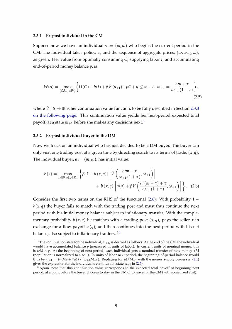
2.3.1 Ex-post individual in the CM
Suppose now we have an individual s := (m, ω) who begins the current period in the
CM. The individual takes policy, τ, and the sequence of aggregate prices, (ω, ω+1, ...),
as given. Her value from optimally consuming C, supplying labor l, and accumulating
end-of-period money balance y, is
W(s) = max(C,l,y)∈R3
+
{U(C)− h(l)+ βV (s+1) : pC+ y ≤ m+ l, m+1 =
ωy + τ
ω+1 (1 + τ)
},
(2.5)
where V : S→ R is her continuation value function, to be fully described in Section 2.3.3
on the following page. This continuation value yields her next-period expected total
payoff, at a state m+1 before she makes any decisions next.9
2.3.2 Ex-post individual buyer in the DM
Now we focus on an individual who has just decided to be a DM buyer. The buyer can
only visit one trading post at a given time by directing search to its terms of trade, (x, q).
The individual buyer, s := (m, ω), has initial value:
B(s) = maxx∈[0,m],q∈R+
{β [1− b (x, q)]
[V(
ωm + τ
ω+1 (1 + τ), ω+1
)]+ b (x, q)
[u(q) + βV
(ω (m− x) + τ
ω+1 (1 + τ), ω+1
)]}. (2.6)
Consider the first two terms on the RHS of the functional (2.6): With probability 1 −b(x, q) the buyer fails to match with the trading post and must thus continue the next
period with his initial money balance subject to inflationary transfer. With the comple-
mentary probability b (x, q) he matches with a trading post (x, q), pays the seller x in
exchange for a flow payoff u (q), and then continues into the next period with his net
balance, also subject to inflationary tranfers. 10
9The continuation state for the individual, m+1, is derived as follows: At the end of the CM, the individualwould have accumulated balance y (measured in units of labor). In current units of nominal money, thisis ωM × y. At the beginning of next period, each individual gets a nominal transfer of new money τM(population is normalized to size 1). In units of labor next period, the beginning-of-period balance wouldthus be m+1 = (ωMy + τM) / (ω+1 M+1). Replacing for M/M+1 with the money supply process in (2.1)gives the expression for the individual’s continuation state m+1 in (2.5).
10Again, note that this continuation value corresponds to the expected total payoff of beginning nextperiod, at a point before the buyer chooses to stay in the DM or to leave for the CM (with some fixed cost).
9
2.3.3 Ex ante decision
At the beginning of a period, before an arbitrary agent s := (m, ω) realizes her DM or
CM market participation status, her value is
V (s) = αW (s) + (1− α)V (s) , (2.7)
where V(s) is the value of playing a fair lottery (π1, 1− π1) over the prizes {z1, z2}, i.e.,
V(s) = maxπ1∈[0,1],z1,z2
{π1V(z1, ω) + (1− π1) V (z2, ω) : π1z1 + (1− π1)z2 = m
}; (2.8)
and, given a lottery outcome z, the individual’s value becomes
V (z, ω) =
maxa∈{0,1} {aW (z− χ, ω) + (1− a) B (z, ω)} , z− χ ≥ −ymax (ω; τ)
B (z, ω) , otherwise,
(2.9)
where
ymax (ω; τ) := min{
m− τ
ω, m}
(2.10)
is a natural upper bound on CM saving (in real money balances). We derive this limit in
the Online Appendix A.
Equation (2.7) says the following: With some exogenous probability α, an agent gets
to enter the frictionless CM costlessly, which will allow him to work and save. The value
of such an event to the individual is W (s). (Note that if the economy were to all exist
as the CM, then there is complete markets insurance of individual consumption risks.)
With probability 1 − α the buyer has to decide whether to enter the CM or DM. Since
the DM-buyer value function may not be strictly concave due to equilibrium externality
from the matching friction, it will be profitable for the individual to play a mixed strategy
over the set of pure actions a ∈ {0, 1}, where a = 0 (a = 1) corresponds to going to
the DM (CM).11 The value to the individual in such an event is V (s), which is defined
by (2.8) and (2.9). Observe that in (2.9), contingent on realizing a lottery payoff z, the
outcome of the lottery also induces the pure action of going to the DM or the CM. Also,
in such (1− α)-measure of contingent events, if the agent decides to go to the CM, he
11The externality problem shows up mathematically as the bilinear and non-concave interaction betweenb (x, q) and u (q) in the DM-buyer’s objective function in (2.6). These two terms, respectively, are inter-pretable as an aggregate extensive margin (i.e., how likely is a buyer to trade) and an intensive margin (i.e.,how much of q to consume).
10
must pay a fixed cost χ ≥ 0 (measured in units of labor) to participate in the CM. This
fixed cost component is interpretable as a barrier to some unlucky and poor individuals
to participate in financial markets (which would have allowed further insurance of their
consumption risks).
Remark 1. Observe that in the ex-ante market participation problem (2.9), there is a limited
short-sale (I.O.U.) constraint z − χ ≥ −ymax (ω; τ). It may be possible that an agent,
whose state is such that m < χ, when faced with deciding to go to the CM, may still find
it optimal to issue an I.O.U. worth m− χ at the beginning of a CM, and go to work in the
CM immediately to repay the shortfall m − χ. Since the fixed cost is levied in the CM,
and in the CM promises or contracts are completely sustainable, then a limited amount of
short selling (I.O.U.) is possible. The limit on the short sale m− χ, is equivalent to agents
exerting the maximal CM labor effort lmax (ω; τ) and not saving anything in the CM. In
Online Appendix B we derive this limit of −ymax (ω; τ) ≡ −min {m, m− τ/ω}.From this we have the following insights:
1. The higher the fixed cost χ, the closer the agent will be to violating this bound,
which means that he will then choose not to participate in the CM.
2. Observe also that, the short-selling limit tightens with higher money supply growth
rate, τ, but loosens with higher ω (but ω may depend positively on τ in equilib-
rium).
Thus, inflation (through money supply growth τ) can create an equilibrium tension act-
ing on the extensive margin of CM participation. (We discuss this again in Section 3.4 on
page 27.)
2.3.4 Special cases
Note that when α = 1 (i.e., agents get to enter the CM deterministically), χ = 0 (there is no
fixed cost of entering the CM), and the continuation value from CM is a convexification
of B(·, ω), our model becomes a version of Lagos and Wright (2005) with competitive
search markets, instead of search with Nash bargaining.
If we retain, the same DM buyer’s problem as we have here, then the economy trivially
collapses to a frictionless CM every period, and we would have a first-best represtative-
agent competitive equilibrium in which money is inessential.
Also, when α = 0, there is no fixed cost of entering the CM (χ = 0), U (C) = 0 for all
C, and the labor utility function h(l) is strictly convex, we recover the original Menzio et
al. (2013) model as a special case.
11
2.4 Monetary equilibrium (ME)
Clearly there exists a non-monetary equilibrium whereby no agent will participate in the
DM. In this paper, we restrict attention to the case of a monetary equilibrium. Hereinafter,
whenever we refer to “monetary equilibrium”, or “equilibrium”, we mean a recursive
monetary equilibrium—one in which agent’s decision functions are recursive and time-
invariant maps. In what follows, we first characterize the equilibrium strategy of firms
(section 2.4.1), the equilibrium value and decision functions of agents in the CM (section
2.4.2) and in the DM (section 2.4.3), and then close the equilibrium notion by describ-
ing the market clearing conditions (section 2.4.4). At the end of this section, we restrict
attention to and define formally the notion of a steady-state or stationary monetary equi-
librium (SME).
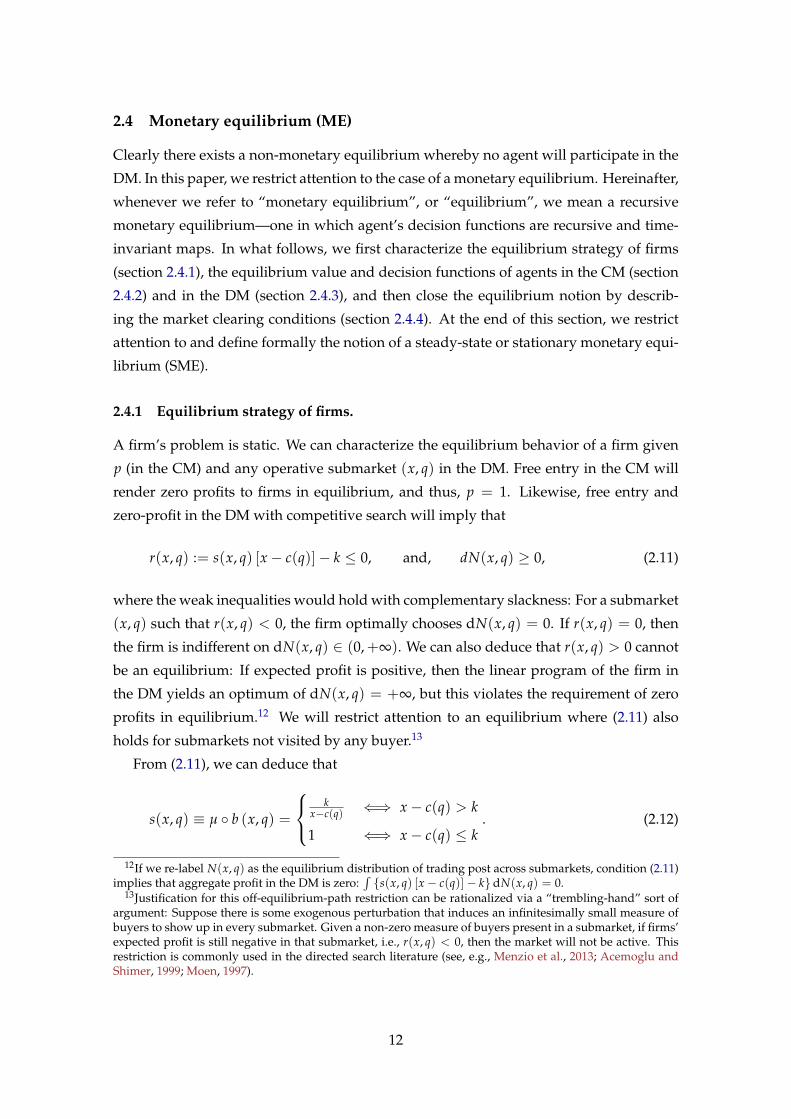
2.4.1 Equilibrium strategy of firms.
A firm’s problem is static. We can characterize the equilibrium behavior of a firm given
p (in the CM) and any operative submarket (x, q) in the DM. Free entry in the CM will
render zero profits to firms in equilibrium, and thus, p = 1. Likewise, free entry and
zero-profit in the DM with competitive search will imply that
where the weak inequalities would hold with complementary slackness: For a submarket
(x, q) such that r(x, q) < 0, the firm optimally chooses dN(x, q) = 0. If r(x, q) = 0, then
the firm is indifferent on dN(x, q) ∈ (0,+∞). We can also deduce that r(x, q) > 0 cannot
be an equilibrium: If expected profit is positive, then the linear program of the firm in
the DM yields an optimum of dN(x, q) = +∞, but this violates the requirement of zero
profits in equilibrium.12 We will restrict attention to an equilibrium where (2.11) also
holds for submarkets not visited by any buyer.13
From (2.11), we can deduce that
s(x, q) ≡ µ ◦ b (x, q) =
k
x−c(q) ⇐⇒ x− c(q) > k
1 ⇐⇒ x− c(q) ≤ k. (2.12)
12If we re-label N(x, q) as the equilibrium distribution of trading post across submarkets, condition (2.11)implies that aggregate profit in the DM is zero:
∫{s(x, q) [x− c(q)]− k}dN(x, q) = 0.
13Justification for this off-equilibrium-path restriction can be rationalized via a “trembling-hand” sort ofargument: Suppose there is some exogenous perturbation that induces an infinitesimally small measure ofbuyers to show up in every submarket. Given a non-zero measure of buyers present in a submarket, if firms’expected profit is still negative in that submarket, i.e., r(x, q) < 0, then the market will not be active. Thisrestriction is commonly used in the directed search literature (see, e.g., Menzio et al., 2013; Acemoglu andShimer, 1999; Moen, 1997).
12
Observe that the firm’s probability of matching with a buyer, s(x, q) depends only on the
posted terms of trade (x, q). Likewise, the buyer’s probability of matching with a firm,
b(x, q), given the matching technology µ : [0, 1] → [0, 1]. Thus, in any submarket with
positive measure of buyers, the market tightness, θ(x, q) ≡ b(x, q)/s(x, q), is neccessarily
and sufficiently determined by free entry into the submarket. Moreover, the terms of
trade of a submarket (x, q) is sufficient to identify the submarket.
It will be convenient for later to note that we have in equilibrium, implicitly, a relation
between q and (x, b). That is, in any equilibrium, each active trading post will produce
and trade the quantity:
q = Q(x, b) ≡ c−1[
x− kµ(b)
], (2.13)
given payment x and its matching probability s = µ(b). This relation will allow us to
perform a change of variable, and re-write the buyers’ problems below in terms choices
over (x, b), instead of over (x, q).
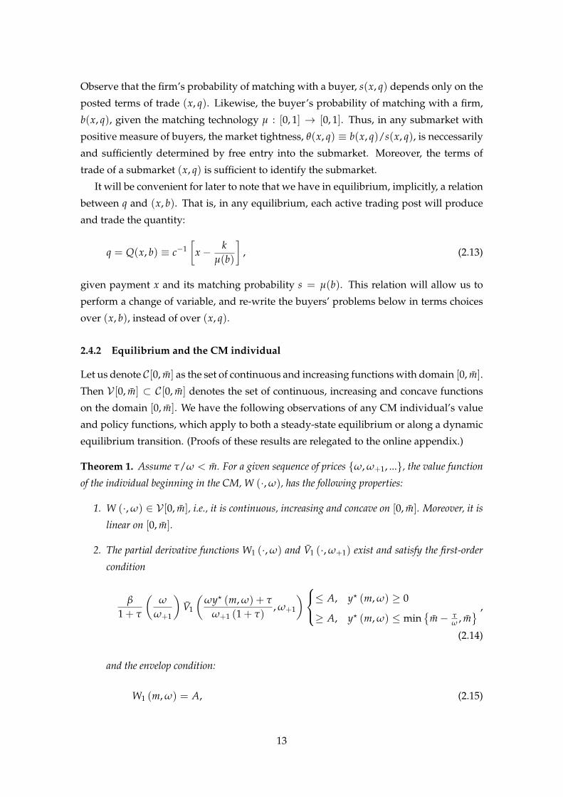
2.4.2 Equilibrium and the CM individual
Let us denote C[0, m] as the set of continuous and increasing functions with domain [0, m].
Then V [0, m] ⊂ C[0, m] denotes the set of continuous, increasing and concave functions
on the domain [0, m]. We have the following observations of any CM individual’s value
and policy functions, which apply to both a steady-state equilibrium or along a dynamic
equilibrium transition. (Proofs of these results are relegated to the online appendix.)
Theorem 1. Assume τ/ω < m. For a given sequence of prices {ω, ω+1, ...}, the value function
of the individual beginning in the CM, W (·, ω), has the following properties:
1. W (·, ω) ∈ V [0, m], i.e., it is continuous, increasing and concave on [0, m]. Moreover, it is
linear on [0, m].
2. The partial derivative functions W1 (·, ω) and V1 (·, ω+1) exist and satisfy the first-order
condition
β
1 + τ
(ω
ω+1
)V1
(ωy? (m, ω) + τ
ω+1 (1 + τ), ω+1
)≤ A, y? (m, ω) ≥ 0
≥ A, y? (m, ω) ≤ min{
m− τω , m
} ,
(2.14)
and the envelop condition:
W1 (m, ω) = A, (2.15)
13
where y?(m, ω) = m + l?(m, ω)− C?(m, ω), l?(m, ω) and C∗(m, ω), respectively, are
the associated optimal choices on labor effort and consumption in the CM.
3. The stationary Markovian policy rules y? (·, ω) and l? (·, ω) are scalar-valued and contin-
uous functions on [0, m].
(a) The function y? (·, ω), is constant valued on [0, m].
(b) The optimizer l? (·, ω) is an affine and decreasing function on [0, m].
(c) Moreover, for every (m, ω), the optimal choice l?(m, ω) is interior: 0 < lmin ≤l? (m) ≤ lmax (ω; τ) < +∞, where there is a very small lmin > 0 and lmax (ω; τ) :=
min{
m− τω , m
}+ U−1 (A) < 2U−1 (A) ∈ (0, ∞).
In the proof to Theorem 1, we also derive the equilibrium decisions of the CM agent.
We show that in an equilibrium, CM consumption is
C? (m, ω) ≡ C? = (U1)−1 (pA) , (2.16)
a finite and non-negative constant. Equilibrium CM asset decision will depend on the
aggregate state ω, i.e.,
y? (m, ω) = y? (ω) (2.17)
and this satisfies the first-order condition (2.14). Finally, from the budget constraint, we
can obtain the equilibrium labor supply function as
l?(m, ω) = C? + y? (ω)−m. (2.18)
Note that l?(m, ω) is single-valued, continuous, affine and decreasing in m.
2.4.3 Equilibrium DM buyer
Observe that since V(·, ω), W(·, ω) ∈ V [0, m] (i.e., are continuous, increasing and con-
cave), then by (2.7), V (·, ω) ∈ V [0, m]. In an equilibrium, the DM buyer’s problem in
(2.6) can be re-written as
B(s) = maxx∈[0,m],b∈[0,1]
{β(1− b)
[V(
ωm + τ
ω+1 (1 + ω), ω+1
)]+ b[
u ◦ Q(x, b) + βV(
ω (m− x) + τ
ω+1 (1 + τ), ω+1
)]}. (2.19)
It appears as if the buyer is choosing his matching probability b along with payment x.
However this is just a change of variables utilizing the equilibrium relation (2.13) between
14
quantity q and terms of trade (x, b). From this we can begin to see that there will be a
trade-off to the buyer, in terms of an extensive margin (i.e., trading opportunity b), and,
an intensive margin (i.e., how much to pay x).
The operator defined by (2.19) clearly does not preserve concavity: The objective func-
tion in (2.19) is not jointly concave in the decisions (x, b) and state m, since it is bilinear in
the function b and the value function V, or the flow payoff function u. However, we can
still show that the resulting DM buyers’ optimal choice functions for (x, b), denoted by
(x?, b?), are monotone, continuous, and have unique selections, using lattice program-
ming arguments.
The following theorem summarizes the properties of a DM agent’s value and policy
functions:14
Theorem 2 (DM value and policy functions). For a given sequence of prices {ω, ω+1, ...}, the
following properties hold.
1. For any V(·, ω+1) ∈ V [0, m], the DM buyer’s value function is increasing and continuous
in money balances, B (·; ω) ∈ C [0, m].
2. For any m ≤ k, DM buyers’ optimal decisions are b? (m, ω) = x? (m, ω) = q? (m, ω) =
0, and B (m, ω) = βV [φ(m, ω), ω+1], where φ(m, ω) := (ωm + τ)/ [ω+1(1 + τ)].
3. At any (m, ω), where m ∈ [k, m] and the buyer matching probability is positive b? (m, ω) >
0:
(a) The optimal selections (x?, b?, q?) (m, ω) and φ?(m, ω) := φ [m− x? (m, ω) , ω],
are unique, continuous, and increasing in m.
(b) The buyer’s marginal valuation of money B1(m, ω) exists if and only if V1 [φ(m, ω), ω]
exists.
(c) B(m, ω) is strictly increasing in m.
(d) the optimal policy functions b?and x?, respectively, satisfy the first-order conditions
u ◦Q [x?(m, ω), b?(m, ω)] + b?(m, ω) (u ◦Q)2 [x?(m, ω), b?(m, ω)]
14Theorem 2 is a generalization of the observation of Menzio et al. (2013) in two aspects: (i) We haveadditional endogenous CM participation in our model; and (ii) the theorem extends beyond steady stateequilibria to encompass equilibrium along a dynamic transition.
15
We prove these results in parts in the online appendix. Part 1 of the Theorem is ob-
tained in Lemma 1, Part 2 is proven as Lemma 2. Part 3(a) is proven as Lemma 3. Lem-
mata 4 and 5 together establish Parts 3(b) and 3(c). Finally, Lemma 6 establishes Part
3(d).
2.4.4 Market clearing
Goods in CM. In equilibrium, the total production of CM good equals its demand:
Y = C ≡ U−1 (A) .
Goods in DM. Given equilibrium policy functions, x? and b?, and, equilibrium distri-
bution of money G and wage ω, equation (2.13) pins downs market clearing for each sub-
market in the set of equilibrium submarkets {(x(m, ω), b(m, ω)) : m ∈ supp(G(·, ω))} .
Labor market clearing. The demand for labor from CM is Y since the firm has a linear
production using labor. All other labor available in the economy must be absorbed by
the firms operating in the DM submarkets. Let zji ≡ zj
i(m, ω) denote the possible lottery
payout, where {1, 2} 3 i denotes the set of the low and the high prize, from playing a
lottery j ∈ J,(
πj1, π
j2
), that spans an arbitrary given individual m at the beginning of the
DM. Thus the measure of buyers at each i = 1, 2 and each j ∈ J is:
Mb(i, j; ω) = (1− α)πji
(zj
i ; ω)
.
Given the constant returns to scale matching function µ, the outcome of market tight-
ness θ in a given submarket satisfies the restriction
bµ(b)
=Ms
Mb≡ θ.
for any respective buyer and seller matching probability outcomes, b and s = µ(b). From
this we can work out the measure of trading posts created in equilibrium to meet buyers
16
with holdings zji as
Ms(i, j; ω) =b?(
zji ; ω)
µ[b?(
zji ; ω)]Mb(i, j; ω)
=b?(
zji ; ω)
µ[b?(
zji ; ω)] (1− α)π
ji
(zj
i ; ω)
.
Since a firm hires workers to create a trading post and to produce outcome q at each
given submarket (x, q), its expected demand for labor is k + c(q)µ [b(x, q)]. Applying the
zero-profit condition (2.11), we also have that
k + c([q?(
zji ; ω)]
µ[b?(
zji ; ω)]
= x?(
zji ; ω)
µ[b?(
zji ; ω)]
,
where again, (q?, b?, x?) are equilibrium Markovian policy functions.
Thus, total demand for labor, across all possible submarkets created in equilibrium is:
∑j∈J
∑i∈{1,2}
Ms(i, j; ω)x?(
zji ; ω)
.
Therefore, we can write the total demand for labor in the economy as:
LD (ω) = Y + ∑j∈J
∑i∈{1,2}
Ms(i, j; ω)x?(
zji ; ω)
= Y + (1− α)∑j∈J
∑i∈{1,2}
b?(
zji ; ω)
πji
(zj
i ; ω)
x?(
zji ; ω)
. (2.22)
Define the indicator function for any agent m ∈ supp(G(·, ω)):
I{m,CM} :=
1 if m goes to CM now
0 otherwise.
On the labor supply side, we have that
LS (ω) =∫
I{m,CM}l?(m, ω)dG(m; ω)
Given the optimal labor supply of agents in the CM, l∗(m; ω) derived in (A.6), aggregate
labor supplied can be re-written as
LS (ω) =∫
I{m,CM}
[C? +
y? (ω) + τ
1 + τω−m
]dG(m; ω) (2.23)
17
The equilibrium wage rate ω is determined by equating (2.22) and (2.23):
τ
1 + τω=
1∫I{m,CM}dG(m; ω)
[Y + (1− α)∑
j∈J∑
i∈{1,2}b?(
zji ; ω)
πji
(zj
i ; ω)
x?(
zji ; ω)]
−[
C? +y? (ω)
1 + τω
]+
∫I{m,CM}mdG(m; ω)∫I{m,CM}dG(m; ω)
. (2.24)
By Walras’ Law, the requirement that all markets described above clear implies that
money demanded must also equal money supplied:
1ω
=∫
mdG(m; ω) > 0. (2.25)
Since M is the beginning of period aggregate stock of money in circulation, then the LHS
of (2.25), 1/ω = M × 1/ωM, is the beginning of period real aggregate stock of money,
measured in units of labor. The RHS of (2.25) is beginning of period aggregate demand,
or holdings, of real money balances measured in the same unit.
2.5 Existence of a SME with unique distribution
For the rest of the paper, we focus on a stationary monetary equilibrium (SME), which
comprises the characterizations from Section 2.4, where the sequence of prices are con-
stant: ω = ω+1.
Definition 1. A stationary monetary equilibrium (SME), given exogenous monetary policy
τ, is a
• list of value functions s 7→ (W, B, V)(s), satisfying the Bellman functionals: (2.5),
(2.6), and jointly, (2.7)-(2.9);
• a list of corresponding decision rules s 7→ (l?, y?, b?, x?, q?, z?, π?)(s) supporting the
value functions;
• a market tightness function s 7→ µ ◦ b?(s) given a matching technology µ, satisfying
firms’ profit maximizing strategy (2.12) and (2.13) at all active trading posts;
• an ergodic distribution of real money balances G(s) satisfying an equilibrium law
of motion
T(G)(E) =∫
P(s, E)dG(s) ∀E ∈ E (2.26)
where, E is Borel σ-algebra generated by open subsets of the product state space S,
and, s 7→ P(s, ·) is a Markov kernel induced by (l?, x?, q?, z?, π?) and µ ◦ b?under τ;
and,
18
• a wage rate function s 7→ ω(s) satisfying labor market clearing (2.24), or equiva-
lently, the money stock adding up condition (2.25).
Computationally, it will be easier to work with condition (2.25) instead of (2.24). At
this point, we note that it will not be difficult to show that there is a unique distribution
of agents in a SME. However, whether a SME is unique remains elusive to us as the
frequency function dG(m; ω) does not admit a closed form expression in terms of known
functions, and in general, it will also depend on the equilibrium candidate ω. 15
The following theorem ensures that in our computations below there exists a steady
state, stationary monetary equilibrium, and for each steady state equilibrium ω, there is
a unique distribution of agents.
Theorem 3. There is a steady-state SME with a unique nondegenerate distribution G.
Proof. First, we show that the value functions listed in the definition of a SME are unique
given ω. For given ω, The CM agent’s problem in (2.5) clearly defines a self-map TCMω :
V [0, m] → V [0, m], which preserves monotonicity, continuity and concavity (see The-
orem 1). However, for fixed ω, the DM buyer’s problem in 2.19 defines an operator
TDMω : V [0, m] → C [0, m], where C [0, m] ⊃ V [0, m] is the set of continuous and increas-
ing functions on the domain [0, m]. This operator does not preserve concavity. Note
that V(·, ω) ∈ V [0, m] as previously defined. Now we show that the ex-ante problem in
(2.9) and (2.8) defines an operator that maps the CM agent’s and the DM buyer’s value
set of continuous, increasing and concave functions: Tω : V [0, m] → V [0, m]. Since
15This statement is also true for the original Menzio et al. (2013) setting, if the authors’ model had moneysupply growth. The intractability of their version of the frequency function dG(m; ω) under money supplygrowth comes about from the modeller no longer being able to work out analytically how long it will take forDM-unmatched buyers’ balances to get eroded by inflation, before they have to go to work again. In contrast,the variation in Sun and Zhou (2016) admits an analytical form for dG(m; ω) and as a result they can showthat there is a unique SME. This special result arises from their assumption that all types of agents in theDM must deterministically enter the CM after one round of trade (or no trade) in the DM, so that the totallabor demand in their model—i.e., their counterpart of equation (2.24)—can be analytically described bya composition of equilibrium decision functions with well-behaved properties and an assumed exogenousdistribution of CM preference shocks. In their model, without an exogenous distribution of CM preferenceshocks, given the market timing assumptions, there would be no distribution of agents since preferences arequasilinear in their CM.
Our setting yields a modelling trade-off in the opposite direction: In contrast to Sun and Zhou (2016),we do not require the latter assumption to preserve distributional non-degeneracy. However, our relaxationhere would come at an analytical cost on the form of the frequency function dG(m; ω). In our opinion, theloss of tractability in this respect is not too severe: Our equilibrium characterization remains computationalfeasible. In fact, it retains the feature that agents’ decision rules depend on the aggregate state only insofaras the scalar aggregate variable, ω. This is because, unlike heterogeneous-agent neoclassical growth modelsor random matching models, the market clearing conditions in competitive search do not require the con-jecture of an entire distribution of assets in order to pin down terms of trade. In that sense, our algorithmfor finding a SME will be similar to that used for computing neoclassical heterogeneous-agent models. Infact, with aggregate shocks (e.g., to τ) our setting will also imply an accurate application of the (originallyheuristic) Krusell and Smith (1998) algorithm to an exact problem. (A similar point was previously discussedin Menzio et al. 2013, pp.2294-2295.)
19
TCMω and TDM
ω are monotone functional operators that satisfy discounting with factor
0 < β < 1, then the ex-ante problem in (2.9) and (2.8), which defines the composite oper-
ator Tω : V [0, m]→ V [0, m], clearly preserves these two properties. (The convexification
of the graph of Tω via lotteries in (2.8) preserves concavity of the image of the operator,
thus making it a self-map on V [0, m].) It can be shown that V [0, m] is a complete metric
space. Thus Tω : V [0, m] → V [0, m] satisfies Blackwell’s conditions, and has a unique
fixed point, V (·, ω) = TωV (·, ω), by Banach’s fixed point theorem.
Second, we verify the following three properties: (1) By Theorem 1 and Theorem 2,
the agent’s optimal policies are continuous, single-valued and monotone functions. This
implies, for fixed ω, that the Markov kernel P(s, ·) in the distributional operator (2.26)
is a probability measure, and, P(·, E) for all Borel subsets E ∈ B ([0, m]) is a measur-
able function. (2) Since agent’s policies are monotone, then P(s, ·) is increasing on [0, m].
Thus the Markov kernel is a transition probability function. (3) The equilibrium policies
clearly dictate that the monotone mixing conditions of Hopenhayn and Prescott (1992)
are satisfied: Consider a DM buyer who has zero money balance. With non-zero proba-
bility either by pure luck (α) or by choosing a lottery that induces such an outcome, he
will enter the CM to work and to accumulate some positive money balance. Likewise,
consider an agent, either in the DM or CM with the highest possible initial balance of m.
Again, with non-zero probability, she will decumulate that balance, either by matching
and spending that balance down in the DM, or, by working less and consuming more in
the CM. These conditions, are sufficient, by Theorem 2 of Hopenhayn and Prescott (1992),
for the Markov operator (2.26) to have a unique fixed point—i.e., regardless of an initial
distribution of agents, the recursive operation on the initial distribution converges (in the
weak* topology) to the same long run distribution G.16
Third, the market clearing condition (2.25) is continuous on the RHS: (1) The integrand
is clearly continuous in m; and, (2) the distribution G (·; ω) is continuous in ω in the sense
of convergence in the weak* topology (Stokey and Lucas, 1989, Theorem 12.13)—i.e., if
ωn → ω?, then for each ωn ∈ {ωn}n∈N, the Markov operator (2.26) defines a (weakly)
convergent sequence of distributions: G (·; ωn) → G (·; ω?). The LHS of (2.25) is clearly
continuous in ω. Thus a SME exists.
3 Computational equilibrium analyses
Finding a SME requires numerical computation. In this section, we parametrize the
model and then we illustrate the dynamic behavior of an individual agent in a economy
in the case where we have positive inflation. We will pause to discuss the underlying
16Alternatively, one could check the more relaxed set of necessary and sufficient conditions of Kamihigashiand Stachurski (2014, Theorem 2) to guarantee that there is a unique distribution for a given ω, in a steadystate SME.
20
forces and trade-offs at work that help will help us to understand the SME outcomes.
This will also help guide our understanding at the end of this section, where we pro-
vide some comparative SME analyses in terms of allocative, distributional and welfare
outcomes.
3.1 Parametrization
The CM and DM preference functions are, respectively,
U (C) = UCM(C + cmin)
1−σCM − (cmin)1−σCM
1− σCM, and, u (q) =
(q + qmin)1−σDM − (qmin)
1−σDM
1− σDM.
Without loss, we set cmin = qmin = 0.001 and normalize σDM = 1.01. The matching
function is such that µ(b) = 1− b. All the parameters of the model are listed in Table 1.
A 1 - Scale on labor disutility functionm 0.95×U−1(A) labor See assumption (2.3)χ 0.1× m = 0.095 labor Fixed cost of CM participationα 0 - Probability of costless CM entryk 0.05 labor Fixed cost of creating a trading post
UCM 0.002 - CM preference scale parameter
Caveat emptor: We plan to estimate some key parameters via the method of simulated
moments (SMM) later. For now, Table 1 contains an ad-hoc parametrization of the model.
3.2 A novel computational scheme
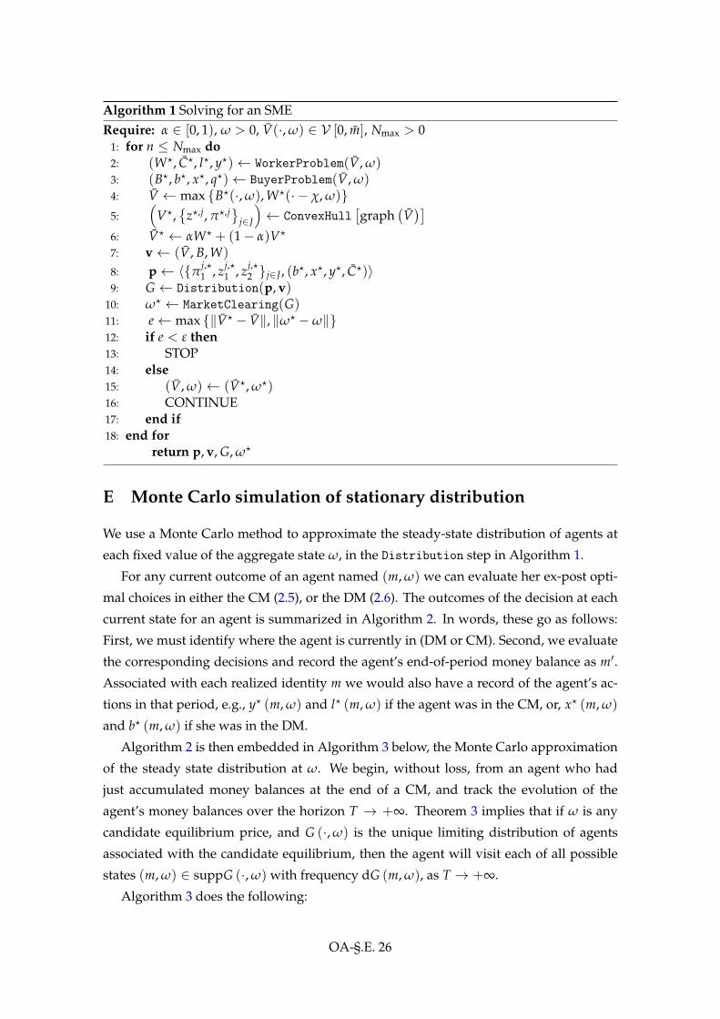
We solve for a steady state SME following the pseudocode in our Online Appendix D.
Our solution method uses a novel insight that refines the computation of the value of the
lottery problem. Recall that the directed search problem makes the ex-ante value function
V(·, ω) non-concave. Since there may exist lotteries that make agents better off than play-
ing pure strategies over participating in DM (as buyer) or CM (as consumer/worker), we
have to devise a means for finding these lotteries that convexify the graph of the function
V (·, ω).17
17Interestingly, there is parallel similarity between our problem here and those in computational dynamicgames. In the latter, non-convexities may sometimes arise in equilibrium payoff sets, and convexificationof these payoff correspondence images are required as a consequence of public randomization, instead oflotteries or behavior strategies (see, e.g., Kam and Stauber, 2016).
21
An existing way to do this in the literature is to use a grid Mg := {0 < · · · < m}to approximate the function’s original domain of [0, m]. Then, around each finite ele-
ment of Mg, one must check if there is a linear segment that approximately convexifies
graph[V (·, ω)
].18 This approximation scheme works fine when we only have a lottery
where the lower bound in Mg is included, i.e., a lottery on a set like {z1, z2}, where z1 = 0,
and, z2 < m. It becomes less accurate when lotteries may exist on upper segments of the
function, i.e., lotteries on sets like {z′1, z′2}, where 0 < z′1 < z′2 < m, but we have no prior
knowlege of what z′1 is. This is because in practice (on the computer) it is not feasible to
implement this check which is meant to be done at every element on the domain [0, m],
not its approximant Mg. As a result, its implementation on Mg may be prone to intro-
ducing non-negligible approximation errors, especially when the mesh of Mg is coarse.
Thus, one would have to make Mg very fine, but, this will come at the cost of the overall
SME solution time.
Instead, we propose a novel alternative here. We can exploit the property that V (·, ω)
has a bounded and convex domain, so then there exists a smallest convex set that con-
tains gV := graph[V (·, ω)
], i.e., conv
(gV),. This set is indeed graph [V (·, ω)]. We
utilize SciPy’s interface to the fast QHULL algorithm to back out a finite set of coordi-
nates representing the convex hull, i.e., graph [V (·, ω)]. Given these points, we approx-
imate the function V (·, ω) by interpolation on a chosen continuous basis function. We
use the family of linear B-splines available from SciPy’s interpolate class for this pur-
pose. As a residual of this exercise, we can very quickly and directly determine the entire
set of possible lotteries that exists with minimal loss of precision, for any given non-
convex/concave function V (·, ω). Detailed comments on how this is done can be found
in the method V in our Python class cssegmod.py.19
3.3 Example SME by simulation
We provide two examples of the previous discussion in Figure 1 on the next page. In Fig-
ure 1(a), we plot the SME value functions (V, B, W) when τ = 0 (i.e., zero steady state in-
flation rate). In Figure 1(b), we have the SME value functions (V, B, W) when τ = 0.1 (i.e.,
10% steady state inflation rate). In both instances of SME, the algorithm finds that only
one lottery segment exists. The solid blue line is the graph of W (·, ω). The dashed green
line is the graph of B (·, ω). The upper envelop of these two graphs give us V (·, ω), the
18See part (v) of the proof of Theorem 3.5 in Menzio et al. (2013) for an exact theoretical underpinning ofthis scheme. We thank Amy Sun for sharing her MATLAB code for Menzio et al. (2013) which confirms thisusage.
19We implement our solution in pure Python 2.7/3.4 (with OpenMPI parallelization of the agent decisionproblems on 20 logical cores). We have only tested our solutions on a Dell Precision T7810 workstation (withIntel Xeon E5-2680 v3, 2.50GHz, processors) running on the Centos 7.2 GNU/Linux operating system. Inall our experiments, we have monotone convergence towards a unique SME solution, regardless of initialguesses on ω and V (·, ω). The average time taken to find the SME is between 90 to 120 seconds, given ourhardware setting.
22
thick solid green line. Denote conv {·} as the convex-hull set operator. The solid magenta
graph is the graph of V (·, ω) obtained through our convex-hull approximation scheme,
once we have located all the intersecting coordinates between the set graph[V (·, ω)
Sustaining these equilibrium value functions are the policy functions (l?, b?, x?, q?)
and the lottery policy with prizes (z1, z2) and lottery (π1, 1− π1) over the prize support,
where π1 (m, ω) = (z2 −m) / (z2 − z1). For example, comparing the cases in Figure 1,
when τ = 0.1, the high prize of z1 = 0.55 is smaller than its counterpart of 0.57 when
τ = 0. Higher anticipated inflation reduces the lottery payoffs since the real value of
money balances get eroded by higher inflation. Also, as expected, higher anticipated
inflation will shift the value functions down uniformly.
The other policy functions can be seen in Figure 2 on the following page. Consider the
panel depicting the graph of the CM labor supply function. As shown earlier in (2.18),
labor supply is affine and decreasing in money balance. There are two shaded patches
in the Figure’s panels. The earth-red patch corresponds to the region where m ∈ [0, k),
i.e., an agent will never match nor trade in the DM. The orange patch (which overlaps
the earth-red patch) is the region of the agent’s state space in which a lottery may be
played—i.e, [z1, z2] 3 m, where in this instance, z1 = 0. What matters for each agent in the
SME is then the loci of these policy functions outside of the orange patch, but including
the points on its boundary. These will be consistent with the equilibrium’s ergodic state
space of agents. As proven in Theorem 2, the policy functions (b?, x?, q?) are monotone
in m in the relevant subspace where an agent can exist at any point in time. The relevant
ergodic subspace of [0, m] in equilibrium is given by {z1, [z2, m]} = {0, [0.55, m]} in the
example of τ = 0.1 in Figure 1(b) or Figure 2.
23
Figure 2: Markov policy functions with τ = 0.1
Given the information about a particular SME’s active or relevant agent state space,
and, the corresponding policy functions, we can use Monte Carlo methods to simulate
an agent’s outcomes. To do so, one may begin from any initial agent named (m, ω) and
apply the decision rules computed earlier, as in Figure 2. Details of how this is done can
be found in our Online Appendix E. This is also relevant for constructing an approxima-
tion of the SME’s probability distribution over agent states. In our solution method, we
simulate an agent over T = 104 periods to approximate the SME’s ergodic distribution.
Figure 3 on the next page shows a subsample of an agent’s existence, for the base-
line economy with monetary policy τ = 0.1. Corresponding to the DM/CM patterns
of spending, we can also observe the subsample’s evolution of money balances, in the
panel with its vertical axis labelled m, in Figure 3. Here, we can see that at t = 0, the
agent has his initial real balance as some m ≈ 0.87. He decides be in the DM, succeeds
in matching with a trading post, and spends a fraction of the balance to consume some
positive q. In the following period t = 1, he begins with some positive balance—because
of transfer τ/(ω (1 + τ)) > 0 combined with his residual balance—but this amount land
in the lottery region; and so the agents plays the lottery. He realizes the high prize of
z2 = 0.57 in t = 1, and so his money balance is z2. He matches and gets to consume
q > 0. (Hence, the record q1, x1, b1 > 0.) A similar event realizes again in t = 2, so the
agent again gets to consume in the DM. In t = 3, having spent his balance on consuming
in the DM the previous period, the agent realizes a low, i.e., z1 = 0, lottery payoff and his
initial balance is thus zero. However, the agent is able to borrow against his CM income,
24
and thus decides to take a temporary short asset position of −χ (although his recorded
money balance is m = z1 = 0) and enters the CM to work, repay the entry cost, consume
in the CM, and save some money balance.20 That is why we see a record of −1 for the
figure panel labelled “match status” for t = 3. Subsequently in t = 4, he begins again
with positive balance from the last CM trade. At this point, he decides to go shopping in
the DM and again, spends it all in one round. he wins the high prize in the lottery, and
finds it profitable to pay the fixed cost χ, enters the CM and works.
Figure 3: Agent sample path (τ = 0.1). Match Status: 0 (No Match in DM), 1 (Match inDM), −1 (in CM).
20See our earlier Remark 1 on page 11.
25
In summary, we can observe the following about this example economy: Agents can
trade more than once in the DM sometimes. This depends on their luck of the draw in
their lottery decisions. Agents must also ocassionally pay a fixed cost to enter the CM
to load up on money balances. Depending on their money balance, they may sometimes
find it worthwhile to borrow against their CM income to pay the fixed cost of CM entry.
Thus, we have an equilibrium Baumol-Tobin style of money demand in the model. Be-
cause agents endogenously may not have complete consumption insurance, the pattern
of consumption, for example, DM q in Figure 3 on the previous page, is not completely
smooth. (While not shown, the same would occur in terms of CM consumption.)
The long run distribution of the sample path of m is shown in Figure 4, for the two
cases of τ = 0 and τ = 0.1. Observe that in each case, the agents, in terms of money
balance m can only spend time in the equilibrium’s ergodic subspace of the set of money
holding. For example this equilibrium subspace turns out to be {z1, [z2, m]} = {0, [0.55, m]},when τ = 0. Comparing between the stationary distribution of SME(τ = 0) in Figure 4(a)
and SME(τ = 0.1) in Figure 4(b), we see that when inflation is higher, more individuals
get stuck with zero balances but also, more agents tend to stay at the top end of the distri-
bution. Comparing this with the sample path of m from Figure 3 on the preceding page,
we can see that with higher inflation, an individual tends to stay for more periods in the
CM, which explains the additional measures of people near the natural upper bound on
money balances in the money distribution in Figure 4(b), in contrast with Figure 4(a).
26
(a) τ = 0 (0% inflation)
(b) τ = 0.1 (10% inflation)
Figure 4: Money distribution under different equilibrium inflation rates
3.4 Mechanism tear-down
We would like to explain the mechanism behind the previous simulation observations,
and, behind the welfare and redistributive consequences of inflation to be shown later.
Since the equilibrium solution is non-analytic, we can at least identify the opposing forces
underlying the effect of inflation on a corresponding SME.
CM-participation intensive vs. extensive margins. Positive inflation has the following
trade-offs: On on hand, with inflation individuals would like to visit the CM more fre-
quently to work and consume there (since in the CM money is not needed for exchange).
On the other hand, given a real fixed cost χ > 0 of entering the CM, higher inflation
means that low-balance agents in the DM will be more unlikely to pay χ to enter the
CM. This is because of two possibilities: (i) their natural short-sale constraints in (2.9)
may be violated if inflation is too high, i.e., m − χ < −ymax (ω; τ) < 0, and so they
choose to stay in the DM and are more likely to keep realizing a bad draw of the zero
27
balance lottery prize; or (ii) their short-sale constraints in (2.9) are not binding, but the
value of going to CM, W (m− χ, ω) is still dominated by the value of going to the DM,
B (m, ω). Nevertheless, in order to continue deriving consumption value in the DM, an
agent would also need to ensure that he has sufficient balance to pay to go back to the
CM often enough to maintain enough precautionary saving of money.
So these trade-offs imply two margins for a precautionary motive for agents with
respect to incomplete consumption insurance: Either they work harder each time in the
CM and bear the cost of holding excess money balances (intensive labor-CM margin), or,
they work less in each CM instance, reduce their spending in each DM exchange, and
ensure that they are more likely to be able to afford to go to the CM frequently (extensive
labor-CM margin).
DM-specific intensive vs. extensive margins. There is another trade-off with respect
to the DM not present in standard general equilibrium models of money, or, in ran-
dom matching models. Consider the equilibrium description of firms’ optimal behavior
in relation to DM production and profit maximization (2.13). Given the firms’ best re-
sponse in a SME, we can deduce the following about a potential DM buyer: Q1(x, b) > 0,
Q2(x, b) < 0, Q(x, b) is weakly concave, and Q12(x, b) = 0. In words, we have another
tension here: On one hand, faced with a given probability of matching with a trading
post, b, the more a buyer is willing to pay, x, the more q she can consume. (This is the in-
tensive margin of DM trade—i.e., how much one can purchase.) On the other hand, given
a required payment, x, a buyer who seeks to match with higher probability, b, must tol-
erate eating less q (This is the extensive margin of DM trade—i.e., trading opportunities.)
From Theorem 2, we know that if a DM buyer brings in more (less) money balance ev-
ery period, then x will be higher (lower) and b will be higher (lower). But the tension just
outlined above gives an ambiguous resolution on q. Thus the intensive (x or q) margin
faces a countervailing force in the intensive margin (b).
All together now. We now consider some numerical results to resolve the CM-participation
and the DM-specific intensive-versus-extensive tensions, in the face of higher inflation.
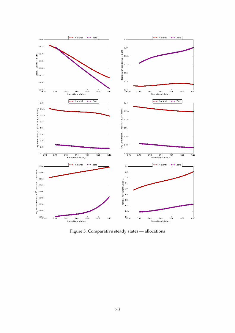
Let us begin with the red-cross graphs in the panels in Figure 5, from left to right,
and, top to bottom. These correspond to economies with the natural borrowing limit
ymax (ω; τ) as defined in (2.10). (The purple-square graphs correspond to alternative
economies with an ad-hoc zero borrowing constraint assumption, where we set ymax (ω; τ) =
0 as in Aiyagari-Huggett type economies.) On the horizontal axes of the panels, we are in-
creasing the steady-state inflation rate, τ ∈ (β− 1, 0.1]. On the vertical axes, we measure
the average outcomes for each corresponding economy’s equilibrium allocation under
policy τ; we denote each equilibrium as SME(τ). For agents who participate in the CM
28
to accumulate money wealth, higher anticipated inflation τ will tend to reduce their la-
bor effort whilst increasing their CM participation rate (i.e., the CM-participation extensive
margin dominates), and they tend to spend (x) and consume (q) less, conditional on find-
ing a match with a trading post, in favor of increasing the likelihood of trading in the
DM (b)—i.e., the DM extensive margin dominates. Because less labor is supplied to firms
in each market, the equilibrium nominal wage per total stock of money (i.e., normalized
nominal wage), ω, increases with τ.
In terms of aggregate and distribution outcomes, higher τ results in lower aggregate
money holdings. In Figure 6, both mean and median money holdings fall with inflation.
Inflation tends to increase wealth inequality (Gini index rises) despite reducing the left-
skewness of the money wealth distribution. Note that higher anticipated inflation affects
agents unequally since they are risk aversion: Higher inflation means relatively lower
(higher) marginal valuation of money to high (low)-balance agents. On one hand, higher
inflation (through both the the CM- and the DM-intensive margin) provides a redistribu-
tion of wealth from high-money-balance agents to low-money-balance agents. Hence,
the less (negative) skewness of the money distribution as inflation rises. Other the hand
(through both the CM- and the DM-extensive margin), inflation raises the downside risk
of agents not getting matched in subsequent trade rounds, and, also raises the cost of
not being able to participate in CM as much, and these two effects imply higher-balance
agents tend to trade “faster” in DM sub-markets by spending and consuming less in
each, and exiting the DM faster. The results shown in Figure 6 suggest that the extensive
margins dominate. The less negative skewness of the distribution under higher inflation,
for example, suggests that the extensive margin is offsetting the rich-to-poor redistributive
aspect of inflation through the intensive channels.
Now we can contrast the economies with the natural borrowing limit with their coun-
terparts with a zero-borrowing limit assumption. Respectively, these are the red-crossed
versus the purple-crossed graphs in Figures 5 and 6. Interestingly, in the economies
where we have imposed the ad-hoc borrowing limit, agents tend to spend less time in
the DM (and more time in the CM), and work less in the CM. In equilibrium, because
agents know they can borrow against their future CM income to pay for the cost of enter-
ing the CM, they choose to work less—or equivalently, hold less money as precaution for
its use in the DM—but as a result, they get much lower consumption in equilibrium. As
a result average welfare is lower in economies with the no-borrowing assumption, but,
money-balance inequality is also lower.
29
Figure 5: Comparative steady states — allocations
30
Figure 6: Comparative steady states — distribution
3.5 Welfare cost of inflation
From the last comparative steady-state exercise, we can also work out the aggregate wel-
fare cost of inflation. For example, to measure mean welfare we consider the ex-ante
mean value
Zτ :=∫
V(m, ω; τ)dG(m, ω; τ).
For a chosen reference economy, SME(τ0) with ex-ante average value as Zτ0 , for any
other SME(τ) we define a welfare measure as compensating equivalent variation in CM
consumption measure:
CEV (τ|τ0) =
[U−1 (Zτ)
U−1 (Zτ0)− 1]× 100%.
We plot this welfare measure across each SME with increasing long run inflation rates.
From Figure 7, we see that the mean welfare measure attain an optimum for some small,
negative inflation rate. This is away from the usual Friedman rule that says optimal
inflation is at β− 1, because of the additional market incompleteness arising for agents
31
not being able to trade in the CM completely and also not being able to trade all the time
in the DM.
Consider the left-hand panel of Figure 7. In this thought experiment, we show the
mean welfare cost of inflation for two settings: natural-borrowing (red-crosses) and zero-
borrowing (purple-squares) limit economies. In the zero-borrowing economies, inflation
reduces welfare more than the natural borrowing-limit economies. The intuition is ob-
vious: In the former, agents are worse off since they face an additional no-borrowing
constraint.
Now consider the right-hand panel of Figure 7. In this thought experiment, we con-
trast an economy where the fixed cost of CM participation, χ, is zero, with a setting
where χ = 0.3. The outcomes are depicted as the blue-circle graph for the former, and
as green-diamond graphs for the latter. A higher fixed cost of CM participation would
amplify the extensive margins outlined earlier. As a consequence, the graphs depicting
CM market participation and average matching probability, for each SME(τ), shift down
with higher χ. Also average consumption, q, and spending, x, in the DM are also lower
with χ, since agents find it more costly to enter the CM, and so must economize on their
money holdings. As a consequence, aggregate money balances shift down with χ. The
effect on wealth inequality is not so clear.
Overall, the welfare statistic tends fall with positive inflation. For the baseline parametriza-
tion of the model (red-squares), relative to the reference economy at τ0 ↘ β− 1 , would
cost welfare in terms of a reduction in equivalent consumption by about 0.2 percent a
quarter, or 0.8 percent per annum. This cost rises to about 1.4 percent per annum if the
fixed cost were χ = 0.3. Or, this welfare cost rises to about 1.6 percent per annum if
agents cannot borrow against their CM incomes to participate in the CM.
Figure 7: Comparative steady states — welfare
32
4 Conclusion
In companion projects (Kam and Lee, 2016; Kam et al., 2016), we explore the dynamics of
the model and also study unanticipated monetary policy shocks.
References
Acemoglu, Daron and Robert Shimer, “Efficient Unemployment Insurance,” Journal of
Political Economy, 1999, 107, 893–928. Cited on page(s): [12]
Bailey, Martin J., “The Welfare Cost of Inflationary Finance,” Journal of Political Economy,
1956, 64 (2), 93–110. Cited on page(s): [3]
Berge, Claude, Topological Spaces, Oliver and Boyd, 1963. Cited on page(s): [OA-§.C. 8]
Burdett, Kenneth, Shouyong Shi, and Randall Wright, “Pricing and Matching with Fric-
tions,” Journal of Political Economy, 2001, 109 (5), 1060–1085. Cited on page(s): [4]
Chiu, Jonathan and Miguel Molico, “Liquidity, Redistribution, and the Welfare Cost of
Inflation,” Journal of Monetary Economics, 2010, 57 (4), 428 – 438. Cited on page(s): [3]
Dotsey, Michael and Peter Ireland, “The welfare Cost of Inflation in General Equilib-
rium,” Journal of Monetary Economics, 1996, 37 (1), 29 – 47. Cited on page(s): [3]
Hopenhayn, Hugo A and Edward C Prescott, “Stochastic Monotonicity and Stationary
Distributions for Dynamic Economies,” Econometrica, November 1992, 60 (6), 1387–406.
Cited on page(s): [20]
Imrohoroglu, Ayse and Edward C. Prescott, “Evaluating the Welfare Effects of Al-
ternative Monetary Arrangements,” Quarterly Review, 1991, (Sum), 3–10. Cited on
page(s): [3]
and , “Seigniorage as a Tax: A Quantitative Evaluation,” Journal of Money, Credit and
Banking, August 1991, 23 (3), 462–75. Cited on page(s): [3]
Julien, Benoît, John Kennes, and Ian King, “Bidding for Money,” Journal of Economic
Fix C? (m, ω) ≡ C?. Since y?c (m, ω) is usc on [0, m], then for all ε ∈ [0, δ], and taking
δ ↘ 0, there exists a selection y? (m− ε, ω) ∈ y?c (m− ε, ω) feasible to a CM agent m.
Similarly, there is a y? (m, ω) ∈ y?c (m, ω) that is feasible to a CM agent m− ε. Moreover,
if l? (m, ω) ∈ l?c (m, ω) is an optimal selection associated with y? (m, ω), then for an agent
OA-§.A. 3
at m,
W (m, ω) = U (C?)− Al? (m, ω) + βV[
ω [m + l? (m, ω)− C?] + τ
ω+1 (1 + τ), ω+1
]︸ ︷︷ ︸
≡Z[m,y?(m,ω)]
≥ U (C?)− Al? (m− ε, ω) + βV[
ω [m + l? (m− ε, ω)− C?] + τ
ω+1 (1 + τ), ω+1
]︸ ︷︷ ︸
≡Z[m,y?(m−ε,ω)]
;
and, for an agent at m− ε,
W (m− ε, ω)
= U (C?)− Al? (m− ε, ω) + βV[
ω [(m− ε) + l? (m− ε, ω)− C?] + τ
ω+1 (1 + τ), ω+1
]︸ ︷︷ ︸
≡Z[m−ε,y?(m−ε,ω)]
≥ U (C?)− Al? (m, ω) + βV[
ω [(m− ε) + l? (m, ω)− C?] + τ
ω+1 (1 + τ), ω+1
]︸ ︷︷ ︸
≡Z[m−ε,y?(m,ω)]
.
Rearranging these inequalities, we have the following fact:
Z [m, y? (m− ε, ω)]− Z [m− ε, y? (m− ε, ω)]
m− (m− ε)
≤ W (m, ω)−W (m− ε, ω)
m− (m− ε)≤ Z [m, y? (m, ω)]− Z [m− ε, y? (m, ω)]
m− (m− ε),
which, after simplifying the denominator and taking limits, yields:
limε↘0
{Z [m, y? (m− ε, ω)]− Z [m− ε, y? (m− ε, ω)]
ε
}≤ lim
ε↘0
{W (m, ω)−W (m− ε, ω)
ε
}≤ lim
ε↘0
{Z [m, y? (m, ω)]− Z [m− ε, y? (m, ω)]
ε
}⇐⇒
β limε↘0
V[
ω(m+l?(m−ε,ω)−C?)+τω+1(1+τ)
, ω+1
]− V
[ω(m−ε+l?(m−ε,ω)−C?)+τ
ω+1(1+τ), ω+1
]ε
≤W1 (m, ω)
≤ β limε↘0
V[
ω(m+l?(m,ω)−C?)+τω+1(1+τ)
, ω+1
]− V
[ω(m−ε+l?(m,ω)−C?)+τ
ω+1(1+τ), ω+1
]ε
.
Since, from (A.3), W (·, ω) is clearly differentiable with respect to m, the second term in
the inequalities above is equal to the partial derivative W1 (m, ω), which is constant. As
ε ↘ 0, there is a selection l? (m− ε, ω) → l? (m, ω), and, by Rockafellar (1970, Theorem
OA-§.A. 4
24.1) the first is the left derivative of V (·, ω+1). Moreover, the last term is identical to the
first, i.e.,
β
1 + τω
(ω
ω+1
)V1
[ω (m− + l? (m, ω)− C?) + τ
ω+1 (1 + τ), ω+1
]≤ W1 (m, ω) ≤ β
1 + τω
(ω
ω+1
)V1
[ω (m− + l? (m, ω)− C?) + τ
ω+1 (1 + τ), ω+1
].
Therefore, if the optimal selection is interior, these weak inequalities must hold with
equality, so we have the left derivative of V with respect to the agent’s decision variable
y as:
β
1 + τω
(ω
ω+1
)V1
[ωy?− (m, ω) + τ
ω+1 (1 + τ), ω+1
]= W1 (m, ω) .
where y?− (m, ω) ≡ m− + l? (m, ω)− C?.
By similar arguments, we can also prove that the right directional derivative of V (·, ω+1)
exists, and show that the right derivative of V with respect to the agents decision y as:
β
1 + τω
(ω
ω+1
)V1
[ωy?+ (m, ω) + τ
ω+1 (1 + τ), ω+1
]= W1 (m, ω) ,
where y?+ (m, ω) ≡ m+ + l? (m, ω)− C?. From the last two equations, we can conclude
that the right and left directional derivatives must agree, and thus, we have the first-order
KKT condition (2.14) as, repeated here as
β
1 + τ
(ω
ω+1
)V1
(ωy? (m, ω) + τ
ω+1 (1 + τ), ω+1
)≤ A, y? (m, ω) ≥ 0
≥ A, y? (m, ω) ≤ min{
m− τω , m
} ,
where the weak inequalities apply with complementary slackness.21 Also, note that in
21Consider the feasible choice set for CM saving y: If m is an upper bound on end-of-period balanceplus transfer (measured in units of labor), then this gives the bounds on end-of-period money balance plustransfer, in current money value, as:
τM ≤ ωMy + τM ≤ ωMm,
where ωM is current nominal wage. Since there is inflation in nominal wage, then next-period initial balanceis current end-of-period nominal money balance normalized by the next period nominal wage M+1ω+1, i.e.,
τMω+1 M+1
≤ m+1 ≡ωMy + τM
ω+1 M+1≤ min
{ωMm
ω+1 M+1, m}
.
Using (2.1), we can re-write the above bounds as
0 ≤ y ≤ min{
m− τ
ω, m}≡ ymax (ω; τ) ,
which applies in the pair of KKT complementary slackness conditions (2.14). Note that the min operator isintroduced to account for the possibility that τ < 0.
OA-§.A. 5
the previous proof of Part 1), we have established the envelop condition (2.15):
W1 (m, ω) = A.
(Part 3.) Observe that given the assumption in (2.3), we have (A.5) always binding:
U′ (C) = pA. Also, observe from(A.5) and (2.14) that an individual’s current money
holding m and the aggregate state ω have no influence on his optimal decision on con-
sumption, C? (m, ω) = C?, but that y? (m, ω) = y? (ω). However, from the budget con-
straint, m clearly does affect the optimal labor decision,
l?(m, ω) = pC? (m, ω) + y? (m, ω)−m
≡(p=1)
C? + y? (ω)−m. (A.6)
Clearly, l?(m, ω) is single-valued, continuous, affine and decreasing in m.
Finally, we show that the optimal choice of l will always be interior. Evaluating the
budget constraint in terms of optimal choices at the current individual state m,
l? (m, ω) = y? (ω)−m + C?.
Since m ∈ [0, m], then, the minimal l attains when m is maximal at m, and, y? (m, ω) = 0:
lmin : = l? (m, ω) ≡ 0− m + C? > 0.
The last inequality obtains from (2.3) which requires m < U−1 (A), and from optimal
CM consumption (2.16) which yields C? = U−1 (A), where p = 1 in an equilibrium. The
maximal l attains when m = 0 and y? (0, ω) = ymax (ω; τ):
lmax (ω, τ) := ymax (ω; τ)− 0+ C? = min{
m− τ
ω, m}+U−1 (A) < 2U−1 (A) . (A.7)
Clearly, lmax (ω, τ) < +∞. If we do not have hyperinflation, or, if transfers are not exces-
sively large—i.e., if τ/ω < m—then, lmax (ω, τ) > 0 will be well-defined. So if τ/ω < m,
then we will have an interior optimizer for all m: 0 < lmin ≤ l? (m) ≤ lmax (ω; τ) <
+∞.
B Limited short-sale constraint and CM participation
Here we derive the short-sale constraint that may bind in the ex-ante market participation
problem (2.9) in the paper. Suppose an agent were to participate in the CM with initial
asset a = z− χ, where z is his ex-ante money balance, and, χ is the fixed cost (in units of
labor) of CM participation. Thus if a < 0, the agent is said to be short selling, or issuing
OA-§.B. 6
an I.O.U.
Recall the CM budget constraint is
y + C = l + a.
The most negative an asset position the agent can attain in an equilibrium is some a such
that he must work at the maximal amount lmax (ω; τ) and cannot afford to save, y = 0.
From the budget constraint in such an equilibrium, we have:
0 + C? = lmax (ω; τ) + a,
which then implies that a = C? − lmax (ω; τ). From (A.7), we can further obtain the
simplified expression a = −ymax (ω; τ) ≡ −min {m, m− τ/ω}. Thus the limited short-
sale constraint in (2.9) in the paper.
C DM agent’s problem
In this section, we provide the omitted proofs leading up to Theorem 2 on page 15 in the
paper. Part 1 of the Theorem is obtained in Lemma 1, Part 2 is proven as Lemma 2. Part
3(a) is proven as Lemma 3. Lemmata 4 and 5 together establish Parts 3(b) and 3(c) of the
Theorem. Finally, Lemma 6 establishes Part 3(d) of the Theorem.
C.1 DM buyer optimal policies
Recall the DM buyer’s problem from (2.19):
B(s) = maxx∈[0,m],b∈[0,1]
{ f (x, b; m, ω)} ,
where
f (x, b; m, ω) := β(1− b)[
V(
ωm + τ
ω+1 (1 + τ), ω+1
)]+ b[
uQ(x, b) + βV(
ω (m− x) + τ
ω+1 (1 + τ), ω+1
)],
and, we have re-defined the composite function u ◦ Q as uQ. Note that we have not
explicitly written f (x, b; m, ω) as depending on ω+1 which is taken as parametric. In an
equilibrium, ω+1 will be recursively dependent on ω, thus our small sleight of hand here
in writing f (x, b; m, ω).
The following Lemmata 1, 2, 3, 4, 5, and 6 make up Theorem 2. Also, these results will
rely on the following statements and notations:
OA-§.C. 7
1. Assume {ω, ω+1, ω+2...} is a given sequence of prices.
2. Let
φ(m, ω) : =ωm + τ
ω+1(1 + τ),
and,
φ?(m, ω) = φ [m− x?(m, ω), ω] .
3. Equivalently define the objective function f (·, ·; m, ω) in the DM buyer’s problem
(2.19) as follows:
f (x, b; m, ω) = βV(
ωm + τ
ω+1 (1 + τ), ω+1
)+ b
[uQ(x, b) + βV (φ?(m, ω), ω+1)− βV (φ(m, ω), ω+1)
].
≡ βV (φ(m, ω), ω+1) + bR (x, b; m, ω) . (C.1)
Remark. Observe that maximizing the value of the objective function f (x, b; m, ω) in the
DM buyer’s problem (2.19) is equivalent to maximizing the second term, bR (x, b; m, ω).
Note that the function R (x, b; m, ω) has the interpretation of the DM buyer’s surplus from
trading with a particular trading post named (x, b), by offering to pay x in exchange for
quantity Q(x, b).
Lemma 1. For any V(·, ω+1) ∈ V [0, m], the DM buyer’s value function is increasing
and continuous in money balances, B (·; ω) ∈ C [0, m].
Proof. Since the functions W (·, ω+1) , V (·, ω+1) ∈ C [0, m], i.e., are continuous and in-
creasing on [0, m], and V := αW + (1− αV), then V (·, ω+1) ∈ C [0, m]. The feasible
choice set Φ(m) := [0, m]× [0, 1] is compact, and it expands with m at each m ∈ [0, m].
By Berge’s Maximum Theorem, the maximizing selections (x?, b?) (m, ω) ∈ Φ(m) exist
for every fixed m ∈ [0, m], since the objective function is continuous on a compact choice
set (Berge, 1963). Evaluating the Bellman operator (2.19), we have that the value function
B (·, ω) ∈ C [0, m].
Lemma 2. For any m ≤ k, DM buyers’ optimal decisions are such that b? (m, ω) = 0
and B (m, ω) = βV [φ(m, ω), ω+1], where φ(m, ω) := ωm+τω+1(1+τ)
.
OA-§.C. 8
Proof. Since a buyer’s payment x is always constrained above by her initial money bal-
ance m in the DM, it will never be optimal for any firm to trade with such a buyer whose
m ≤ k, as the firm will be making an economic loss. In equilibrium it is thus optimal
for a buyer m ≤ k to optimally not trade and exit the DM with end-of-period balance
as m (i.e., with beginning-of-next-period balance φ(m, ω) when inflationary transfers
are accounted for). As a result, the continuation value is V [φ(m, ω), ω+1], and thus,
B (m, ω) = βV [φ(m, ω), ω+1], if m ≤ k.
Lemma 3. For any (m, ω), where m ∈ [k, m] and the buyer matching probability is
positive b? (m, ω) > 0, the optimal selections (x?, b?, q?) (m, ω) and φ?(m, ω) :=
φ [m− x? (m, ω) , ω] are unique, continuous, and increasing in m.
Observe that the DM buyer’s problem has a general structure similar to that of Menzio
et al. (2013). The main difference is in the details underlying the buyer’s continuation
value function, which in our setting is denoted by V (·, ω). Nevertheless, we still have
that V (·, ω) ∈ V [0, m]. As a consequence the proof of Lemma 3.3 in Menzio et al. (2013)
can be adapted to our setting. For the reader’s convenience, we repeat the proof strategy
of Menzio et al. (2013) below for our model setting in a few steps:
Proof. The DM buyer’s problem (2.19) can be re-written as
B(s) = βV (φ(m, ω), ω+1) + exp{
maxx∈[0,m],b∈[0,1]
{ln (b) + ln [R (x, b; m, ω)]}}
.
The optimizers thus must satisfy
(x?, b?)(m, ω) ∈{
arg maxx∈[0,m],b∈[0,1]
{ln (b) + ln [R (x, b; m, ω, ω+)]}}
. (C.2)
(Uniqueness and continuity of policies.) First we establish that the policy functions are con-
tinuous, and, at every state, there is a unique optimal selection: Since uQ (x, b) is contin-
uous, jointly and strictly concave in (x, b), and by assumption, V (·, ω) ∈ V [0, m] , then
R (x, b; m, ω) ≡ uQ(x, b) + βV (φ?(m, ω), ω+1)− βV (φ(m, ω), ω+1)
is continuous, jointly and strictly concave in the choice variables (x, b). Also, ln(b) is
strictly increasing and strictly concave in b. Thus the maximand is jointly and strictly
concave in (x, b). By Berge’s Maximum Theorem, the optimal selections (x?, b?)(m, ω)
are continuous and unique at any m. Since c 7→ c(q) is bijective, then
q?(m, ω) = c−1 [x?(m, ω)− k/µ (b?(m, ω))]
OA-§.C. 9
is continuous in m; and so is φ?(m, ω).
(Monotonicity of policies.) The remainder of this proof establishes that the policy functions
are increasing. The key idea of the proof is in showing that the choice set is a lattice
equipped with a partial order, that the choice set is increasing in m, and, has increasing
differences on the choice set, and the slices of the buyer’s objective is supermodular in
each given direction of his choice set. By Theorem 2.6.2 of Topkis (1998), these properties
are sufficient to ensure that the buyer’s objective function is supermodular. Together,
these properties suffice, by Theorem 2.8.1 of Topkis (1998), for showing that the buyer’s
optimal policies are increasing functions in m.
1. The function R (·, ·, ·, ω) in (C.2) has increasing difference in (x, b, m) and is therefore
supermodular:
Fix an m ∈ [k, m] and b ∈ (0, 1]. (The case of b = 0 is trivially uninteresting.) It
suffices to optimize over the function ln [R (·, b, m, ω)] in (C.2). Then the optimizer
x(b, m, ω) ∈{
arg maxx∈[k,m]
{ln [R (x, b, m, ω)]}}
is unique for each (m, b, ω), since the objective functions is strictly concave.
Next we show how the value of the objective function has increasing differences in
(x, b, m), throughout taking the sequence {ω, ω+1, ...} as fixed. Thus we will now
write R (x, b, m) ≡ R (x, b, m, ω) to temporarily ease the notation. First, the feasible
choice set
Fm : = {(x, b, m) : x ∈ [0, m] , b ∈ [0, 1] , m ∈ [k, m]} ,
is a partially ordered set with relation ≤, and it has least-upper and greatest-lower
bounds. It is therefore a sublattice in R3+. Observe that Fm is increasing in m.
Second, pick any m′ > m, b′ > b, and x′ > x in Fm:
(a) For fixed x, consider m′ > m and b′ > b. Then, we can write
R(
x, b′, m′)− R (x, b, m)
=[uQ(x, b′)− uQ(x, b)
]+ β
[V(
ω (m′ − x) + τ
ω+1 (1 + τ), ω+1
)− V
(ω (m− x) + τ
ω+1 (1 + τ), ω+1
)]− β
[V(
ωm′ + τ
ω+1 (1 + τ), ω+1
)− V
(ωm + τ
ω+1 (1 + τ), ω+1
)].
Observe that the RHS is separable in b and m: The first term on the right,
uQ(x, b′) − uQ(x, b) < 0, shows increasing difference in b. Likewise the re-
OA-§.C. 10
mainder two difference terms on the RHS show increasing differences in m.
Overall R (x, b, m) has increasing differences on the lattice [0, 1] × [0, m] 3(b, m).
(b) For fixed m, consider x′ > x and b′ > b. Observe that
R (x, b, m)− R(x′, b, m
)=[uQ(x, b)− uQ(x′, b)
]+ β
[V(
ω (m− x) + τ
ω+1 (1 + τ), ω+1
)− V
(ω (m− x′) + τ
ω+1 (1 + τ), ω+1
)]. (C.3)
Now, using the expression (C.3) twice below, we have that
[R(x′, b′, m
)− R
(x, b′, m
)]−[R(x′, b, m
)− R (x, b, m)
]=[uQ(x′, b′)− uQ(x, b′)
]+ β
[V(
ω (m− x′) + τ
ω+1 (1 + τ), ω+1
)− V
(ω (m− x) + τ
ω+1 (1 + τ), ω+1
)]−[uQ(x′, b)− uQ(x, b)
]− β
[V(
ω (m− x′) + τ
ω+1 (1 + τ), ω+1
)− V
(ω (m− x) + τ
ω+1 (1 + τ), ω+1
)]=[uQ(x′, b′)− uQ(x, b′)
]−[uQ(x′, b)− uQ(x, b)
]> 0,
where the last inequality is implied by the fact that(uQ)
12 (x, b) > 0. Therefore
R (x, b, m) has increasing differences on the lattice [0, m]× [0, 1] 3 (x, b).
(c) For fixed b, consider x′ > x and m′ > m. Observe that
[R(
x′, b, m′)− R
(x, b, m′
)]−[R(x′, b, m
)− R (x, b, m)
]=[uQ(x′, b)− uQ(x, b)
]+ β
[V(
ω (m′ − x′) + τ
ω+1 (1 + τ), ω+1
)− V
(ω (m′ − x) + τ
ω+1 (1 + τ), ω+1
)]−[uQ(x′, b)− uQ(x, b)
]− β
[V(
ω (m− x′) + τ
ω+1 (1 + τ), ω+1
)− V
(ω (m− x) + τ
ω+1 (1 + τ), ω+1
)]= β
[V(
ω (m′ − x′) + τ
ω+1 (1 + τ), ω+1
)− V
(ω (m′ − x) + τ
ω+1 (1 + τ), ω+1
)]− β
[V(
ω (m− x′) + τ
ω+1 (1 + τ), ω+1
)− V
(m− x + τ
1 + τω, ω+1
)]≥ 0,
where the last weak inequality obtains from the property that V (·, ω+1) ∈V [0, m], and V (·, ω+1) is therefore weakly concave. Therefore R (x, b, m) has
increasing differences on the lattice [0, m]× [0, m] 3 (x, m).
OA-§.C. 11
From parts (1a), (1b), and (1c), we can conclude that the objective function R (·, ·, ·, ω)
has increasing differences on Fm. This suffices to prove that the objective function
R (·, ·, ·, ω) is supermodular (see Topkis, 1998, Corollary 2.6.1), since the domain of
the function is a direct product of a finite set of chains (partially ordered sets with no
unordered pair of elements), and, the objective function is real valued (see Topkis,
1978).
2. Since R (·, b, m) is supermodular, for fixed choice b, the optimizer x (b, m, ω) is in-
creasing in (b, m), for given ω:
Let x (b, m, ω) = arg maxx∈[0,m] R (x, b, m). From part (1a) above, we can deduce
that for fixed x (b, m), R (b, m) ≡ R [x (b, m, ω) , b, m] is supermodular on the lattice
[0, 1]× [0, m] 3 (b, m). Since R(x, b, m) is strictly decreasing in b, then
R (b, m) ≡ R [x (b, m, ω) , b, m]
is strictly decreasing in b. Observe that for any m′ ≥ m, where m′, m ∈ [k, m], we
have
R(x, b, m′
)− R (x, b, m)
= β
[V(
ωm + τ
ω+1 (1 + τ), ω+1
)− V
(ω (m− x) + τ
ω+1 (1 + τ), ω+1
)]− β
[V(
ωm′ + τ
ω+1 (1 + τ), ω+1
)− V
(ω (m′ − x) + τ
ω+1 (1 + τ), ω+1
)]≥ 0,
since V (·, ω) is concave. Since this inequality holds at each fixed pair(x, b), then,
R (b, m) ≡ R [x (b, m, ω) , b, m]
≤ R[x (b, m, ω) , b, m′
]≤ R
[x(b, m′, ω
), b, m′
]≡ R
(b, m′
).
The last weak inequality obtains because the choice set is increasing in m, and so
x (b, m, ω) is a feasible selection for the more relaxed problem whose value is
R[x(b, m′, ω
), b, m′
]= max
x∈[0,m′]R(x, b, m′
).
From these weak inequalities, we can conclude that R (b, m) is increasing in m.
Now we are ready to apply Theorem 2.8.1 of Topkis (1998) to show that b? (m, ω)
increases with m: Let
b? (m, ω) = arg maxb∈[0,1]
r (b, m)
OA-§.C. 12
where r (b, m) = b · R (b, m) and R (b, m) ≡ R (x (b, m, ω) , b, m, ω). Observe the
following identity:
[r(b′, m′
)− r
(b, m′
)]−[r(b′, m
)− r (b, m)
]=
b′{
R(b′, m′
)− R
(b, m′
)−[R(b′, m
)− R (b, m)
]}+(b′ − b
) [R(b, m′
)− R (b, m)
],
for any b, b′ ∈ (0, 1] , m, m′ ∈ [k, m] where b′ > b and m′ > m. The first term on
the RHS is positive, since b′ > 0 and since R (b, m) is supermodular in (b, m), then
Topkis (1998, Theorem 2.6.1) applies, so that R (b, m) has increasing differences on
[0, 1]× [0, m] (i.e., the terms in the curly braces are positive). Since we have previ-
ously established that R (b, m) is increasing in m, and b′ − b > 0, then the second
term on the RHS is also positive. Thus the objective r(b, m) is supermodular on
[0, 1]× [k, m] 3 (b, m). (Note that the choice set of b does not depend on m.)
Therefore, by Theorem 2.8.1 of Topkis (1998), the optimal selection b? (m, ω) is in-
creasing in m. Since x (b, m, ω) is increasing in (b, m), for given ω, then we can
conclude that the optimal payment choice x? (m, ω) = x (b? (m, ω) , m, ω) is also
increasing in m.
3. The decision q? (m, ω) is monotone in m:
We perform a change of decision variables. Denote a ≡ ϕ + c(q), where, ϕ ≡ m− x.
Then we have a change of the DM buyer’s decision variables from (x, q) to (a, q).
From (2.12), we can re-write m − x = a − c(q) and b = µ−1 [k/ (m− a)]. Since
b ∈ [0, 1], the domain of a is [0, m− k], and the domain for q is [0, a]. The buyer’s
problem from (2.19) is thus equivalent to writing
B(m, ω)− βV(
ωm + τ
ω+1 (1 + τ), ω+1
)= max
a∈[0,m−k],q∈[0,a]
{µ−1
(k
m− a
)[u (q)
+βV(
ω (a− q) + τ
ω+1 (1 + τ), ω+1
)− βV
(ωm + τ
ω+1 (1 + τ), ω+1
)]}. (C.4)
Recall we take the sequence (ω, ω+1, ...) as parametric here. This problem can be
broken down into two steps: Fix (a, ω). Find the optimal q for any a, to be denoted
by q (a, ω), and then, find the optimal a given (a, ω), to be denoted by a? (m, ω).
Then we can deduce the optimal q? (m, ω) ≡ q [a? (m, ω) , m, ω]. We details these
steps below:
(a) For any fixed a and (m, ω), q (a, ω) induces the value
J (a, ω) = maxq∈[0,a]
{u (q) + βV
(ω (a− q) + τ
ω+1 (1 + τ), ω+1
)}. (C.5)
OA-§.C. 13
Observe that q and J do not depend on m, given a fixed a. The objective
function on the RHS is clearly supermodular on the lattice [0, m− k]× [0, a] 3(a, q). Since the objective function is strictly concave, the selection q(a, ω) in
unique for every a, given ω. Also, the choice set [0, a] increases with a, and,
the objective function is increasing. Therefore, respectively by Theorems 2.8.1
(increasing optimal solutions) and 2.7.6 (preservation of supermodularity) of
Topkis (1998), we have that q(a, ω) and J(a, ω) are increasing in a.
(b) Given best response q(a, ω), the optimal a? (m, ω) choice satisfies
a? (m, ω) = arg maxa∈[0,m−k]
g (a, m, ω) ,
where
g (a, m, ω) = µ−1(
km− a
) [J (m, ω)− βV
(ωm + τ
ω+1 (1 + τ), ω+1
)].
(Again, note that we have suppressed dependencies on ω+1 since this is taken
as parametric by the agent, and, in equilibrium ω+1 recursively depends on
ω.)
Consider the case J (a, ω) − βV(
ωm+τω+1(1+τ)
, ω+1
)≥ 0. Since µ (b) is strictly
decreasing in b, and 1/µ (b) is strictly convex in b, then µ−1(
km−a
)is strictly
increasing in m, strictly decreasing in a, and is strictly supermodular in (a, m).
Pick any a′, a ∈ [0, m− k], and any m′, m ∈ [k, m], such that a′ > a and m′ > m.
We have the identity:
[g(a′, m′, ω
)− g
(a, m′, ω
)]−[g(a′, m, ω
)− g (a, m, ω)
]=[
µ−1(
km′ − a′
)− µ−1
(k
m− a′
)] [J(a′, ω
)− J (a, ω)
]+
[µ−1
(k
m′ − a
)− µ−1
(k
m′ − a′
)]×[
βV(
ωm′ + τ
ω+1 (1 + τ), ω+1
)− βV
(ωm + τ
ω+1 (1 + τ), ω+1
)]+
[µ−1
(k
m′ − a′
)− µ−1
(k
m′ − a
)− µ−1
(k
m− a′
)− µ−1
(k
m− a
)]×[
J (a, ω)− βV(
ωm + τ
ω+1 (1 + τ), ω+1
)]
The first term on the RHS is positive since µ−1(
km−a
)is strictly increasing in
m, and we have previously shown that J (a, ω) is increasing in a. The sec-
ond term on the RHS is positive since µ−1(
km−a
)is strictly decreasing in a,
OA-§.C. 14
and, V (·, ω) ∈ V [0, m]. The last term on the RHS is positive since µ−1(
km−a
)is supermodular, and therefore its first term in the product shows increasing
differences Topkis (1998, Theorem 2.6.1). Its last term in the product is pos-
itive under the case we are considering. Therefore the LHS is positive, and
this suffices to establish that g (a, m, ω) is strictly supermodular (Topkis, 1998,
Theorem 2.8.1).
Finally, since the choice set [0, m− k] is increasing in m, the solution a? (m, ω)
is also increasing in m Topkis (1998, Theorem 2.6.1). Since we have established
in part (3a) that q (m, ω) is increasing in a, then, q? (m, ω) ≡ q [a? (m, ω) , ω] is
also increasing in m.
4. The decision φ? (m, ω) is monotone in m:
Similar to the procedure in the last part, we perform a change of decision variables
via a ≡ ϕ + c(q), where, ϕ ≡ m− x. The domain for ϕ is [0, min {m, a}]. However,
an optimal choice under b > 0 means that we will have ϕ < m (the end of period
residual balance is less than the beginning of period money balance). This is be-
cause, if ϕ = m then it must be that x = 0, i.e., the buyer pays nothing; but this
is not optimal for the buyer if the buyer faces a positive probability of matching
b > 0. Moreover, ϕ < a, if u′ (0) is sufficiently large—i.e., the buyer can always
increase utility by raising x (thus lowering ϕ such that ϕ < a attains). Thus the
upper bound on ϕ will never be binding. As such, the buyer’s problem from (2.19)
can be re-written as
B(m, ω)− βV(
ωm + τ
ω+1 (1 + τ), ω+1
)= max
a∈[0,m−k],ϕ≥0
{µ−1
(k
m− a
) [uC (a− ϕ)
+βV(
ωϕ + τ
ω+1 (1 + τ), ω+1
)− βV
(ωm + τ
ω+1 (1 + τ), ω+1
)]}, (C.6)
where uC (q) := u ◦ c−1 (q), which is continuously differentiable with respect to
q ≥ 0. For fixed a ∈ [0, m− k], denote the value
J (a, ω) = maxϕ≥0
{uC (a− ϕ) + βV
(ωϕ + τ
ω+1 (1 + τ), ω+1
)}, (C.7)
and the optimizer,
ϕ(a, ω) = arg maxϕ≥0
{uC (a− ϕ) + βV
(ωϕ + τ
ω+1 (1 + τ), ω+1
)}. (C.8)
Denote also q(a, ω) = c−1 [a− ϕ(a, ω)].
OA-§.C. 15
Given ϕ(a, ω), the optimal choice over a, i.e., a? (m, ω), solves
B(m, ω)− βV(
ωm + τ
ω+1 (1 + τ), ω+1
)=
maxa∈[0,m−k]
{µ−1
(k
m− a
) [J (a, ω)− βV
(ωm + τ
ω+1 (1 + τ), ω+1
)]}.
Applying the similar logic in the proof in part 3 on page OA-§.C. 13, we can show
that ϕ(a, ω) is increasing in a; that a? (m, ω) is increasing in m, and therefore, ϕ? (m, ω) ≡ϕ [a? (m, ω) , ω] is increasing in m. Finally, since
φ? (m, ω) : = [ωϕ? (m, ω) + τ] / [ω+1 (1 + τ)] ,
which is a linear transform of ϕ? (m, ω), then φ? (m, ω) is increasing with m, since
ω/ [ω+1 (1 + τ)] > 0.
C.2 DM buyer value function and first-order conditions
Let us return to the DM buyer’s problem re-written as (C.6) in part (4) of the proof of
Lemma 3 on page OA-§.C. 9. The buyer’s decision problem over ϕ ≡ m− x, for any fixed
decision a ≡ ϕ + c(q), yields the value J (a, ω) as defined in equation (C.7) of that proof.
The following intermediate results says that the value function J (·, ω) is differentiable
with respect to a and its marginal value can be related to primitives, i.e.:
Lemma 4. The marginal value of J (·, ω) agrees with the flow DM marginal utility
with respect to the buyer’s payment x,
J1 (a, ω) =u′ [q(a, ω)] ≡(
uQ)
1[x?(m, ω), b?(m, ω)] > 0. (C.9)
Proof. Consider the problem described in equations (C.6) and (C.7). Observe that since
ϕ ≡ a− c (q), then
ϕ(a, ω) = arg maxϕ≥0
{uC (a− ϕ) + βV
(ωϕ + τ
ω+1 (1 + τ), ω+1
)}(C.10)
is continuous with respect to a: There is some δ′ > 0, such that for all ε ∈ [0, δ′], the
choices ϕ(a+ ε, ω) and ϕ(a− ε, ω) exist. Moreover the optimal selection ϕ(a, ω) is unique
since the objective function in (C.10) is strictly concave by virtue of uC being strictly con-
cave and V being concave. Denote also q(a, ω) = c−1 [a− ϕ(a, ω)], where the choices
q(a + ε, ω) and q(a− ε, ω) also exist, by continuity of c−1 in its argument.
OA-§.C. 16
To verify (C.9), we can use the perturbed choices, ϕ(a + ε, ω) and ϕ(a− ε, ω), for eval-
uating right- and left-derivatives of the functions uC, V and J, in order to “sandwich” the
derivative function J1 (·, ω) and arrive at the claimed result. For notational convenience
below, we define the following function
Kω [a, ϕ(a, ω)] ≡ uC (a− ϕ(a, ω)) + βV(
ωϕ(a, ω) + τ
ω+1 (1 + τ), ω+1
).
Consider first the right derivatives: Take δ′ ↘ 0 such that for all ε ∈ [0, δ′], the choice
ϕ(a + ε, ω) is affordable for a buyer a. Since ϕ(·, ω) is an optimal policy satisfying (C.8),
Observe that b? (m, ω) > 0 implies the buyer has more than enough initial balance for
purchasing q? (m, ω), i.e.,
m− ϕ? (m, ω) > c [q?(m, ω)] + k =⇒ a(m, ω) ≡ ϕ? (m, ω) + c [q?(m, ω)] < m− k.
Since a?(m, ω) < m − k, and a?(m, ω) is continuous in m, then there is an ε > 0 such
that the following selections are also feasible: a?(m + ε, ω) < m − k, and, a?(m, ω) <
(m− ε) − k. Define the open ball Nε (m) := (m− ε, m + ε). Note that for any m′ ∈
22Note that b = µ−1(
km−a
). The term db/da = k/ (m− a)2 × 1/µ′ [b] can be derived using the implicit
function theorem: Define H(a, b) = k/ (m− a)− µ [b] = 0. Then db/da = −Ha(a, b)/Hb(a, b), which yieldsthe result. The first-order condition is thus derived as[
J (a?(m, ω), ω)− βV(
ωm + τ
ω+1 (1 + τ), ω+1
)]k
(m− a?(m, ω))21
µ′ [b? (m, ω)]
+ J1 (a?(m, ω), ω) µ−1(
km− a?(m, ω)
){= 0, if a?(m, ω) < m− k< 0, if a?(m, ω) = m− k
.
Moreover, since k/(m − a) = µ(b), we can write db/da = k/ (m− a)2 × 1/µ′ [b] ≡ [µ (b)]2 /k × 1/µ′ [b],and using the relation (C.9), the first-order condition can be further simplified to (C.11).
OA-§.C. 19
Nε (m), the selection a? (m′, ω) is feasible for an agent m; and a? (m, ω) is feasible for
agent m′.
Given that a? (m, ω) is optimal for agent m, and since ϕ?(m, ω) = ϕ [a? (m, ω)], then
we have the buyer’s optimal value as
B(m, ω) = βV(
ωm + τ
ω+1 (1 + τ), ω+1
)+ max
a∈[0,m−k],ϕ≥0
{µ−1
(k
m− a
)×[u ◦ c−1 (a− ϕ) + βV
(ωϕ + τ
ω+1 (1 + τ), ω+1
)− βV
(ωm + τ
ω+1 (1 + τ), ω+1
)}= F (a? (m, ω) , m) ≥ F (a? (m + ε, ω) , m) .
where F (a, m) := βV(
ωm+τω+1(1+τ)
, ω+1
)+µ−1
(k
m−a
) [J (a, ω)− βV
(ωm+τ
ω+1(1+τ), ω+1
)]. Sim-
ilarly, for agent m + ε, it must be that
B (m + ε, ω) = F (a? (m + ε, ω) , m + ε) ≥ F (a? (m, ω) , m + ε) .
Clearly,
F (a? (m, ω) , m + ε)− F (a? (m, ω) , m)
ε≤ B (m + ε, ω)− B (m, ω)
ε
≤ F (a? (m + ε, ω) , m + ε)− F (a? (m + ε, ω) , m)
ε.
Since F (a, m) is continuous and concave in a, and, a? (m, ω) is continuous in m, the fol-
lowing limits exist (Rockafellar, 1970, Theorem 24.1, pp.227-228), and the inequality or-
dering is preserved in the limit:
limε↘0
F (a? (m, ω) , m + ε)− F (a? (m, ω) , m)
ε≤ lim
ε↘0
B (m + ε, ω)− B (m, ω)
ε
≤ limε↘0
F (a? (m + ε, ω) , m + ε)− F (a? (m + ε, ω) , m)
ε.
Since limε↘0 a? (m + ε, ω) = a? (m, ω), the inequalities above are equivalent to
b? (m, ω)
[J1 (a? (m, ω) , ω)− β
1 + τωV1
(ωm+ + τ
ω+1 (1 + τ), ω+1
)]+
β
1 + τωV1
(ωm+ + τ
ω+1 (1 + τ), ω+1
)≤ B1
(m+, ω
)≤ b? (m, ω)
[J1 (a? (m, ω) , ω)− β
1 + τωV1
(ωm+ + τ
ω+1 (1 + τ), ω+1
)]+
β
1 + τωV1
(ωm+ + τ
ω+1 (1 + τ), ω+1
),
OA-§.C. 20
where
V1
(ωm+ + τ
ω+1 (1 + τ), ω+1
):= lim
ε↘0(1 + τ)
(ω+1
ω
) [V(
ω (m + ε) + τ
ω+1 (1 + τ), ω+1
)− V
(ωm + τ
ω+1 (1 + τ), ω+1
)]/ε.
However, observe that the first and the last terms in the inequalities are identical. Thus
we must have that the right derivative of B (·, ω) satisfies
B1(m+, ω
)= b? (m, ω)
[J1 (a? (m, ω) , ω)− β
1 + τ
(ω
ω+1
)V1
(ωm+ + τ
ω+1 (1 + τ), ω+1
)]+
β
1 + τ
(ω
ω+1
)V1
(ωm+ + τ
ω+1 (1 + τ), ω+1
).
By a similar process to arrive at the left derivative of B (·, ω), we have
B1(m−, ω
)= b? (m, ω)
[J1 (a? (m, ω) , ω)− β
1 + τ
(ω
ω+1
)V1
(ωm− + τ
ω+1 (1 + τ), ω+1
)]+
β
1 + τ
(ω
ω+1
)V1
(ωm− + τ
ω+1 (1 + τ), ω+1
),
where
V1
(ωm− + τ
ω+1 (1 + τ), ω+1
):= (1 + τ)
(ω+1
ω
)limε↘0
{1ε
[V(
ω (m− ε) + τ
ω+1 (1 + τ), ω+1
)− V
(ωm + τ
ω+1 (1 + τ), ω+1
)]}.
Using the result from (C.9) in Lemma 4 on page OA-§.C. 16, we can re-write these right-
and left-derivative functions, respectively, as
B1(m+, ω
)= b? (m, ω)
(uQ)
1[x? (m, ω) , x? (m, ω)]
+β [1− b? (m, ω)]
1 + τ
(ω
ω+1
)V1
(ωm+ + τ
ω+1 (1 + τ), ω+1
), (C.12)
and,
B1(m−, ω
)= b? (m, ω)
(uQ)
1[x? (m, ω) , x? (m, ω)]
+β [1− b? (m, ω)]
1 + τ
(ω
ω+1
)V1
(ωm− + τ
ω+1 (1 + τ), ω+1
). (C.13)
From (C.12) and (C.13), it is apparent that B1 (m, ω) exists if and only if the left- and
right-derivatives of V (·, ω+1) exist and they agree at the continuation state from m, i.e.,
OA-§.C. 21
if
V1
(ωm− + τ
ω+1 (1 + τ), ω+1
)= V1
(ωm+ + τ
ω+1 (1 + τ), ω+1
)= V1
(ωm + τ
ω+1 (1 + τ), ω+1
).
This proves the first part of the statement in the Lemma.
Since V (·, ω+1) ∈ V [0, m], it is concave and increasing in m, and therefore,
V1
(ωm− + τ
ω+1 (1 + τ), ω+1
)≥ V1
(ωm+ + τ
ω+1 (1 + τ), ω+1
)≥ 0.
Since we assumed b? (m, ω) ∈ (0, 1], and by Lemma 4, we have
J1 (a? (m, ω) , ω) ≡(
uQ)
1[x? (m, ω) , x? (m, ω)] > 0,
then (C.12) and (C.13) imply that the first-order left and right derivatives of B (·, ω+1)
satisfy:
B1(m−, ω
)≥ B1
(m+, ω
)≥ b? (m, ω)
(uQ)
1[x? (m, ω) , x? (m, ω)] > 0.
From this ordering, we can conclude that if b? (m, ω) > 0, the buyer’s valuation B (m, ω+1)
is strictly increasing with his money balance, m. This proves the last part of the statement
in the Lemma.
Lemma 6. For any (m, ω), where m ∈ [k, m] and the buyer matching probability is
positive b? (m, ω) > 0, the optimal policy functions b?and x?, respectively, satisfy the
first-order conditions (2.20) and (2.21).
Proof. We want to show that the first order conditions characterizing the optimal policy
functions b?and x?, are indeed (2.20) and (2.21). It is immediate that the objective function
(2.19) is continuously differentiable with respect to the choice b ∈ [0, 1]. Holding fixed x,
if the optimal choice for b is interior, b?(m, ω) ∈ (0, 1), then it must satisfies the first order
condition (2.20) with respect to b:
uQ [x?(m, ω), b?(m, ω)] + b?(m, ω)(
uQ)
2[x?(m, ω), b?(m, ω)]
= β [V (φ (m, ω) , ω+1)− V (φ? (m, ω) , ω+1)] .
The first order condition with respect to x is more subtle. We can derive it by first defining
one-sided derivatives of B (·, ω). Assuming beginning-of-next-period residual balance
OA-§.C. 22
after current DM trade is positive—i.e.,
φ? (m, ω) =ω [m− x? (m, ω)] + τ
ω+1 (1 + τ)> 0. (C.14)
Since (C.14) holds, and since we have shown in Lemma 3 that x? (m, ω) and φ? (m, ω) are
continuous in m ∈ [k, m], then
(φ?)+ (m, ω) : =ω [m + ε− x? (m, ω)] + τ
ω+1 (1 + τ),
and,
(φ?)− (m, ω) : =ω [m− ε− x? (m, ω)] + τ
ω+1 (1 + τ),
exist and are feasible (or affordable). From (2.19), the DM buyer’s one-sided derivatives
of B (·, ω)—i.e., its left- or right-marginal valuation of initial money balance—are, respec-
tively,
B1(m+, ω
)=
β
1 + τ
(ω
ω+1
)×{[1− b? (m, ω)] V1
(ωm+ + τ
ω+1 (1 + τ), ω
)+ b? (m, ω) V1
[(φ?)+ (m, ω) , ω+1
]},
(C.15)
and,
B1(m−, ω
)=
β
1 + τ
(ω
ω+1
)×{[1− b? (m, ω)] V1
(ωm− + τ
ω+1 (1 + τ), ω
)+ b? (m, ω) V1
[(φ?)− (m, ω) , ω+1
]},
(C.16)
where
V1
(ωm± + τ
ω+1 (1 + τ), ω+1
):= (1 + τ)
(ω+1
ω
)limε↘0
{1ε
[V(
ω (m± ε) + τ
ω+1 (1 + τ), ω+1
)− V
(ωm + τ
ω+1 (1 + τ), ω
)]}.
From Lemma 5, we have shown by change of variable, that the one-sided derivatives
of B (·, ω) also satisfy (C.15) and (C.16). These are repeated here for convenience as the
OA-§.C. 23
following equations:
B1(m+, ω
)=
β
1 + τ
(ω
ω+1
)[1− b? (m, ω)] V1
(ωm+ + τ
ω+1 (1 + τ), ω
)+ b? (m, ω)
(uQ)
1[x? (m, ω) , b? (m, ω)] , (C.17)
and,
B1(m−, ω
)=
β
1 + τ
(ω
ω+1
)[1− b? (m, ω)] V1
(ωm− + τ
ω+1 (1 + τ), ω
)+ b? (m, ω)
(uQ)
1[x? (m, ω) , b? (m, ω)] . (C.18)
From the last term on the RHS of each of equations (C.15), (C.16), (C.17), and, (C.18), we
have the observation that
β
1 + τ
(ω
ω+1
)V1
[(φ?)+ (m, ω) , ω+1
]=
β
1 + τω
(ω
ω+1
)V1
[(φ?)− (m, ω) , ω+1
]=(
uQ)
1[x? (m, ω) , b? (m, ω)] .
Since these marginal valuation functions are evaluated at the DM buyer’s optimal choice,
it must be that β1+τ
(ω
ω+1
)V1
[(φ?)+ (m, ω) , ω+1
]= β
1+τ
(ω
ω+1
)V1
[(φ?)− (m, ω) , ω+1
]=
β1+τ
(ω
ω+1
)V1 [φ
?(m, ω), ω+1], and, that this satisfies the first order condition (2.21), which
is (uQ)
1[x?(m, ω), b?(m, ω)] =
β
1 + τ
(ω
ω+1
)V1 [φ
?(m, ω), ω+1] .
D Algorithm for finding a SME
We compute a SME as follows.
1. Fix a guess ω and guess V (·, ω) ∈ V [0, m].
2. Solve for CM policy and value functions:
• We know C? (m, ω) = C? already using equation (2.16).
• For fixed C?, and, given guess of V (·, ω), iterate on Bellman equation (A.3)
solving a one-dimensional (1D) optimization problem over choice y? (·, ω).
– Note: By equation (2.17), the solution y? (·, ω) = y∗ (ω) should be a con-
stant with respect to m.
OA-§.D. 24
• Back out l?(m, ω) using the binding budget constraint (2.18).
• Store value function W? (·, ω).
3. Solve for DM policy and value functions:
• For each m ≤ k, set
– b? (m, ω) = x? (m, ω) = q? (m, ω) = 0
– B (m, ω) = βV [φ(m, ω), ω+1],
where φ(m, ω) := (m + τ)/(1 + τω).
• For each m ∈ [k, m],
– Invert first-order condition (2.21) to obtain implicit b [m, x (m, ω) , ω].
– Plug the implicit expression for b [m, x (x, ω) , ω] into Bellman equation
(2.19), and do a 1D optimization over choices x (m, ω).
– Get optimizer x? (m, ω) and corresponding value B? (m, ω) .
– Use previous step to now back out b? (m, ω).
4. Solve ex-ante decision problem:
• Given approximants W? (m, ω) and B? (m, ω), solve the lottery problem (2.9)
and (2.8).
• Get policies{
πj,?1 (m, ω)
}j∈J
and{
zj,?1 (m, ω) , zj,?
2 (m, ω)}
j∈J, where J is en-
dogenous to the solution of (2.9) and (2.8).
• Get value of the problem (2.9) and (2.8) as V? (·, ω).
5. Construct the approximant of the ex-ante value function, V? (·, ω) = (1− α)V? (·, ω)+
αW? (·, ω) .
6. Given policy functions from Steps 2-4, construct limiting distribution G (·, ω) solv-
ing the implicit Markov map (2.26). (See details in Section E on page OA-§.E. 26.)
• Check if market clearing condition (2.25) holds.
• If not,
– generate new guess and set ω ← ωnew;
– set V (·, ω)← V? (·, ω); and
– repeat Steps 2-6 again until (2.25) holds.
Algorithm 1 on page OA-§.E. 26 summarizes the steps above with reference to function
names in our actual Python implementation. Algorithm 1 is called SolveSteadyState in
our Python class file cssegmod.py.
OA-§.E. 25
Algorithm 1 Solving for an SMERequire: α ∈ [0, 1), ω > 0, V(·, ω) ∈ V [0, m], Nmax > 0
1: for n ≤ Nmax do2: (W?, C?, l?, y?)← WorkerProblem(V, ω)3: (B?, b?, x?, q?)← BuyerProblem(V, ω)4: V ← max {B?(·, ω), W?(· − χ, ω)}5:
(V?,
{z?,j, π?,j}
j∈J
)← ConvexHull
[graph
(V)]
6: V? ← αW? + (1− α)V?
7: v← (V, B, W)
8: p← 〈{π j,?1 , zj,?
1 , zj,?2 }j∈J , (b?, x?, y?, C?)〉
9: G ← Distribution(p, v)10: ω? ← MarketClearing(G)11: e← max {‖V? − V‖, ‖ω? −ω‖}12: if e < ε then13: STOP14: else15: (V, ω)← (V?, ω?)16: CONTINUE17: end if18: end for
return p, v, G, ω?
E Monte Carlo simulation of stationary distribution
We use a Monte Carlo method to approximate the steady-state distribution of agents at
each fixed value of the aggregate state ω, in the Distribution step in Algorithm 1.
For any current outcome of an agent named (m, ω) we can evaluate her ex-post opti-
mal choices in either the CM (2.5), or the DM (2.6). The outcomes of the decision at each
current state for an agent is summarized in Algorithm 2. In words, these go as follows:
First, we must identify where the agent is currently in (DM or CM). Second, we evaluate
the corresponding decisions and record the agent’s end-of-period money balance as m′.
Associated with each realized identity m we would also have a record of the agent’s ac-
tions in that period, e.g., y? (m, ω) and l? (m, ω) if the agent was in the CM, or, x? (m, ω)
and b? (m, ω) if she was in the DM.
Algorithm 2 is then embedded in Algorithm 3 below, the Monte Carlo approximation
of the steady state distribution at ω. We begin, without loss, from an agent who had
just accumulated money balances at the end of a CM, and track the evolution of the
agent’s money balances over the horizon T → +∞. Theorem 3 implies that if ω is any
candidate equilibrium price, and G (·, ω) is the unique limiting distribution of agents
associated with the candidate equilibrium, then the agent will visit each of all possible
states (m, ω) ∈ suppG (·, ω) with frequency dG (m, ω), as T → +∞.