750
Numerical Techniques in Electromagnetics Second Edition

NumericalTechniques in
ElectromagneticsSecond Edition

Matthew N. O. Sadiku, Ph.D.
NumericalTechniques in
ElectromagneticsSecond Edition
Boca Raton London New York Washington, D.C.CRC Press

This book contains information obtained from authentic and highly regarded sources. Reprinted materialis quoted with permission, and sources are indicated. A wide variety of references are listed. Reasonableefforts have been made to publish reliable data and information, but the author and the publisher cannotassume responsibility for the validity of all materials or for the consequences of their use.
Neither this book nor any part may be reproduced or transmitted in any form or by any means, electronicor mechanical, including photocopying, microfilming, and recording, or by any information storage orretrieval system, without prior permission in writing from the publisher.
The consent of CRC Press LLC does not extend to copying for general distribution, for promotion, forcreating new works, or for resale. Specific permission must be obtained in writing from CRC Press LLCfor such copying.
Direct all inquiries to CRC Press LLC, 2000 N.W. Corporate Blvd., Boca Raton, Florida 33431.
Trademark Notice:
Product or corporate names may be trademarks or registered trademarks, and areused only for identification and explanation, without intent to infringe.
© 2001 by CRC Press LLC
No claim to original U.S. Government worksInternational Standard Book Number 0-8493-1395-3
Library of Congress Card Number 00-026823Printed in the United States of America 1 2 3 4 5 6 7 8 9 0
Printed on acid-free paper
Library of Congress Cataloging-in-Publication Data
Sadiku, Matthew N. O.Numerical techniques in electromagnetics / Matthew N.O. Sadiku.—[2nd ed.].
p. cm.Includes bibliographical references and index.ISBN 0-8493-1395-3 (alk. paper)1. Electromagnetism. 2. Numerical analysis. I. Title.
QC760 .S24 2000537
′
.01
′
515—dc21 00-026823 CIP

Preface
The art of computation of electromagnetic (EM) problems has grown exponentiallyfor three decades due to the availability of powerful computer resources. In spiteof this, the EM community has suffered without a suitable text on computationaltechniques commonly used in solving EM-related problems. Although there havebeen monographs on one particular technique or the other, the monographs are writtenfor the experts rather than students. Only a few texts cover the major techniques anddo that in a manner suitable for classroom use. It seems experts in this area arefamiliar with one or few techniques and not many experts seem to be familiar withall the common techniques. This text attempts to fill the gap.
The text is intended for seniors or graduate students and may be used for a one-semester or two-semester course. The main requirements for students taking a coursebased on this text are introductory EM courses and a knowledge of a high-levelcomputer language, preferably FORTRAN or C. Software packages such as Matlaband Mathcad may be helpful tools. Although familiarity with linear algebra andnumerical analysis is useful, it is not required.
In writing this book, three major objectives were borne in mind. First, the book isintended to teach students how to pose, numerically analyze, and solve EM problems.Second, it is designed to give them the ability to expand their problem solving skillsusing a variety of available numerical methods. Third, it is meant to prepare graduatestudents for research in EM. The aim throughout has been simplicity of presentationso that the text can be useful for both teaching and self-study. In striving aftersimplicity, however, the reader is referred to the references for more information.Toward the end of each chapter, the techniques covered in the chapter are appliedto real life problems. Since the application of the technique is as vast as EM andauthor’s experience is limited, the choice of application is selective.
Chapter 1 covers some fundamental concepts in EM. Chapter 2 is intended to putnumerical methods in a proper perspective. Analytical methods such as separationof variables and series expansion are covered. Chapter 3 discusses the finite differ-ence methods and begins with the derivation of difference equation from a partialdifferential equation (PDE) using forward, backward, and central differences. Thefinite-difference time-domain (FDTD) technique involving Yee’s algorithm is pre-
v

sented and applied to scattering problems. Numerical integration is covered usingtrapezoidal, Simpson’s, Newton-Cotes rules, and Gaussian quadratures.
Chapter 4 on variational methods serves as a preparatory ground for the next twomajor topics: moment methods and finite element methods. Basic concepts suchas inner product, self-adjoint operator, functionals, and Euler equation are covered.Chapter 5 on moment methods focuses on the solution of integral equations. Chap-ter 6 on finite element method covers the basic steps involved in using the finiteelement method. Solutions of Laplace’s, Poisson’s, and wave equations using thefinite element method are covered.
Chapter 7 is devoted to transmission-line matrix or modeling (TLM). The methodis applied to diffusion and scattering problems. Chapter 8 is on Monte Carlo methods,while Chapter 9 is on the method of lines.
Since the publication of the first edition, there has been an increased awareness andutilization of numerical techniques. Many graduate curricula now include coursesin numerical analysis of EM problems. However, not much has changed in compu-tational electromagnetics. A major noticeable change is in the FDTD method. Themethod seems to have attracted much attention and many improvements are beingmade to the standard algorithm. This edition adds the noticeable change in incorpo-rating absorbing boundary conditions in FDTD, FEM, and TLM. Chapter 9 is a newchapter on the method of lines.
Acknowledgements
I am greatly indebted to Temple University for granting me a sabbatical in Fall 1998during which I was able to do most of the revision. I specifically would like to thankmy dean, Dr. Keya Sadeghipour, and my chairman, Dr. John Helferty, for their support.Special thanks are due to Raymond Garcia of Georgia Tech for writing Appendices Cand D in C++. I am deeply grateful to Dr. Arthur D. Snider of the University ofSouth Florida and Mohammad R. Zunoubi of Mississippi State University for takingthe time to send me the list of errors in the first edition. I thank Dr. Reinhold Preglafor helping in clarifying concepts in Chapter 9 on the method of lines. I expressmy deepest gratitude to my wife, Chris, and our daughters, Ann and Joyce, for theirpatience, sacrifices, and prayers.
A Note to Students
Before you embark on writing your own computer program or using the ones in thistext, you should try to understand all relevant theoretical backgrounds. A computer

is no more than a tool used in the analysis of a program. For this reason, you shouldbe as clear as possible what the machine is really being asked to do before setting itoff on several hours of expensive computations.
It has been well said by A.C. Doyle that “It is a capital mistake to theorize beforeyou have all the evidence. It biases the judgment.” Therefore, you should never trustthe results of a numerical computation unless they are validated, at least in part. Youvalidate the results by comparing them with those obtained by previous investigatorsor with similar results obtained using a different approach which may be analyticalor numerical. For this reason, it is advisable that you become familiar with as manynumerical techniques as possible.
The references provided at the end of each chapter are by no means exhaustive butare meant to serve as the starting point for further reading.

Contents
1 Fundamental Concepts1.1 Introduction 1.2 Review of Electromagnetic Theory
1.2.1 Electrostatic Fields 1.2.2 Magnetostatic Fields 1.2.3 Time-varying Fields 1.2.4 Boundary Conditions 1.2.5 Wave Equations 1.2.6 Time-varying Potentials 1.2.7 Time-harmonic Fields
1.3 Classification of EM Problems1.3.1 Classification of Solution Regions 1.3.2 Classification of Differential Equations 1.3.3 Classification of Boundary Conditions
1.4 Some Important Theorems 1.4.1 Superposition Principle 1.4.2 Uniqueness Theorem References Problems
2 Analytical Methods2.1 Introduction 2.2 Separation of Variables 2.3 Separation of Variables in Rectangular Coordinates
2.3.1 Laplace’s Equations 2.3.2 Wave Equation

2.4 Separation of Variables in Cylindrical Coordinates 2.4.1 Laplace’s Equation 2.4.2 Wave Equation
2.5 Separation of Variables in Spherical Coordinates2.5.1 Laplace’s Equation 2.5.2 Wave Equation
2.6 Some Useful Orthogonal Functions 2.7 Series Expansion
2.7.1 Poisson’s Equation in a Cube 2.7.2 Poisson’s Equation in a Cylinder 2.7.3 Strip Transmission Line
2.8 Practical Applications 2.8.1 Scattering by Dielectric Sphere2.8.2 Scattering Cross Sections
2.9 Attenuation Due to Raindrops2.10 Concluding Remarks
References Problems
3 Finite Difference Methods3.1 Introduction3.2 Finite Difference Schemes 3.3 Finite Differencing of Parabolic PDEs 3.4 Finite Differencing of Hyperbolic PDEs 3.5 Finite Differencing of Elliptic PDEs
3.5.1 Band Matrix Method 3.5.2 Iterative Methods
3.6 Accuracy and Stability of FD Solutions 3.7 Practical Applications I — Guided Structures
3.7.1 Transmission Lines 3.7.2 Waveguides
3.8 Practical Applications II — Wave Scattering (FDTD) 3.8.1 Yee’s Finite Difference Algorithm3.8.2 Accuracy and Stability3.8.3 Lattice Truncation Conditions3.8.4 Initial Fields 3.8.5 Programming Aspects
3.9 Absorbing Boundary Conditions for FDTD 3.10 Finite Differencing for Nonrectangular Systems
3.10.1 Cylindrical Coordinates 3.10.2 Spherical Coordinates
3.11 Numerical Integration 3.11.1 Euler’s Rule3.11.2 Trapezoidal Rule 3.11.3 Simpson’s Rule

3.11.4 Newton-Cotes Rules3.11.5 Gaussian Rules 3.11.6 Multiple Integration
3.12 Concluding Remarks References Problems
4 Variational Methods4.1 Introduction 4.2 Operators in Linear Spaces 4.3 Calculus of Variations4.4 Construction of Functionals from PDEs 4.5 Rayleigh-Ritz Method 4.6 Weighted Residual Method
4.6.1 Collocation Method4.6.2 Subdomain Method4.6.3 Galerkin Method4.6.4 Least Squares Method
4.7 Eigenvalue Problems 4.8 Practical Applications4.9 Concluding Remarks
ReferencesProblems
5 Moment Methods5.1 Introduction5.2 Integral Equations
5.2.1 Classification of Integral Equations5.2.2 Connection Between Differential and Integral Equations
5.3 Green’s Functions 5.3.1 For Free Space 5.3.2 For Domain with Conducting Boundaries
5.4 Applications I — Quasi-Static Problems5.5 Applications II — Scattering Problems
5.5.1 Scattering by Conducting Cylinder 5.5.2 Scattering by an Arbitrary Array of Parallel Wires
5.6 Applications III — Radiation Problems5.6.1 Hallen’s Integral Equation 5.6.2 Pocklington’s Integral Equation 5.6.3 Expansion and Weighting Functions
5.7 Applications IV — EM Absorption in the Human Body 5.7.1 Derivation of Integral Equations 5.7.2 Transformation to Matrix Equation (Discretization) 5.7.3 Evaluation of Matrix Elements 5.7.4 Solution of the Matrix Equation

5.8 Concluding Remarks References Problems
6 Finite Element Method6.1 Introduction 6.2 Solution of Laplace’s Equation
6.2.1 Finite Element Discretization6.2.2 Element Governing Equations 6.2.3 Assembling of All Elements 6.2.4 Solving the Resulting Equations
6.3 Solution of Poisson’s Equation 6.3.1 Deriving Element-governing Equations 6.3.2 Solving the Resulting Equations
6.4 Solution of the Wave Equation 6.5 Automatic Mesh Generation I — Rectangular Domains 6.6 Automatic Mesh Generation II — Arbitrary Domains
6.6.1 Definition of Blocks 6.6.2 Subdivision of Each Block 6.6.3 Connection of Individual Blocks
6.7 Bandwidth Reduction 6.8 Higher Order Elements
6.8.1 Pascal Triangle6.8.2 Local Coordinates 6.8.3 Shape Functions6.8.4 Fundamental Matrices
6.9 Three-Dimensional Elements 6.10 Finite Element Methods for Exterior Problems
6.10.1 Infinite Element Method 6.10.2 Boundary Element Method6.10.3 Absorbing Boundary Conditions
6.11 Concluding RemarksReferencesProblems
7 Transmission-line-matrix Method7.1 Introduction 7.2 Transmission-line Equations 7.3 Solution of Diffusion Equation 7.4 Solution of Wave Equations
7.4.1 Equivalence Between Network and Field Parameters 7.4.2 Dispersion Relation of Propagation Velocity 7.4.3 Scattering Matrix 7.4.4 Boundary Representation 7.4.5 Computation of Fields and Frequency Response

7.4.6 Output Response and Accuracy of Results 7.5 Inhomogeneous and Lossy Media in TLM
7.5.1 General Two-Dimensional Shunt Node 7.5.2 Scattering Matrix 7.5.3 Representation of Lossy Boundaries
7.6 Three-Dimensional TLM Mesh 7.6.1 Series Nodes 7.6.2 Three-Dimensional Node 7.6.3 Boundary Conditions
7.7 Error Sources and Correction 7.7.1 Truncation Error 7.7.2 Coarseness Error 7.7.3 Velocity Error 7.7.4 Misalignment Error
7.8 Absorbing Boundary Conditions 7.9 Concluding Remarks
ReferencesProblems
8 Monte Carlo Methods8.1 Introduction 8.2 Generation of Random Numbers and Variables 8.3 Evaluation of Error8.4 Numerical Integration
8.4.1 Crude Monte Carlo Integration 8.4.2 Monte Carlo Integration with Antithetic Variates8.4.3 Improper Integrals
8.5 Solution of Potential Problems 8.5.1 Fixed Random Walk8.5.2 Floating Random Walk 8.5.3 Exodus Method
8.6 Regional Monte Carlo Methods 8.7 Concluding Remarks
References Problems
9 Method of Lines9.1 Introduction 9.2 Solution of Laplace’s Equation
9.2.1 Rectangular Coordinates9.2.2 Cylindrical Coordinates
9.3 Solution of Wave Equation 9.3.1 Planar Microstrip Structures 9.3.2 Cylindrical Microstrip Structures
9.4 Time-Domain Solution

9.5 Concluding Remarks References Problems
A Vector RelationsA.1 Vector IdentitiesA.2 Vector Theorems A.3 Orthogonal Coordinates
B Solving Electromagnetic Problems Using C++B.1 Introduction B.2 A Brief Description of C++ B.3 Object-Orientation B.4 C++ Object-Oriented Language Features B.5 A Final Note
References
C Numerical Techniques in C++D Solution of Simultaneous Equations
D.1 Elimination Methods D.1.1 Gauss’s Method D.1.2 Cholesky’s Method
D.2 Iterative Methods D.2.1 Jacobi’s Method D.2.2 Gauss-Seidel Method D.2.3 Relaxation Method D.2.4 Gradient Methods . . . .
D.3 Matrix Inversion D.4 Eigenvalue Problems
D.4.1 Iteration (or Power) MethodD.4.2 Jacobi’s Method
E Answers to Odd-Numbered Problems

To my teacher
Carl A. Ventriceand my parents
Ayisat and Solomon Sadiku

Chapter 1
Fundamental Concepts
“Science knows no country because knowledge belongs to humanity and is thetorch which illuminates the world. Science is the highest personification of thenation because that nation will remain the first which carries the furthest theworks of thoughts and intelligence.” Louis Pasteur
1.1 Introduction
Scientists and engineers use several techniques in solving continuum or field prob-lems. Loosely speaking, these techniques can be classified as experimental, analyti-cal, or numerical. Experiments are expensive, time consuming, sometimes hazardous,and usually do not allow much flexibility in parameter variation. However, every nu-merical method, as we shall see, involves an analytic simplification to the point whereit is easy to apply the numerical method. Notwithstanding this fact, the followingmethods are among the most commonly used in electromagnetics (EM).
A. Analytical methods (exact solutions)
(1) separation of variables
(2) series expansion
(3) conformal mapping
(4) integral solutions, e.g., Laplace and Fourier transforms
(5) perturbation methods
B. Numerical methods (approximate solutions)
(1) finite difference method
(2) method of weighted residuals
(3) moment method
(4) finite element method
© 2001 by CRC PRESS LLC

(5) transmission-line modeling
(6) Monte Carlo method
(7) method of lines
Application of these methods is not limited to EM-related problems; they findapplications in other continuum problems such as in fluid, heat transfer, and acous-tics [1].
As we shall see, some of the numerical methods are related and they all generallygive approximate solutions of sufficient accuracy for engineering purposes. Sinceour objective is to study these methods in detail in the subsequent chapters, it may bepremature to say more than this at this point.
The need for numerical solution of electromagnetic problems is best expressed inthe words of Paris and Hurd: “Most problems that can be solved formally (analyti-cally) have been solved.”1 Until the 1940s, most EM problems were solved using theclassical methods of separation of variables and integral equation solutions. Besidesthe fact that a high degree of ingenuity, experience, and effort were required to applythose methods, only a narrow range of practical problems could be investigated dueto the complex geometries defining the problems.
Numerical solution of EM problems started in the mid-1960s with the availabilityof modern high-speed digital computers. Since then, considerable effort has beenexpended on solving practical, complex EM-related problems for which closed formanalytical solutions are either intractable or do not exist. The numerical approach hasthe advantage of allowing the actual work to be carried out by operators without aknowledge of higher mathematics or physics, with a resulting economy of labor onthe part of the highly trained personnel.
Before we set out to study the various techniques used in analyzing EM problems,it is expedient to remind ourselves of the physical laws governing EM phenomenain general. This will be done in Section 1.2. In Section 1.3, we shall be acquaintedwith different ways EM problems are categorized. The principle of superposition anduniqueness theorem will be covered in Section 1.4.
1.2 Review of Electromagnetic Theory
The whole subject of EM unfolds as a logical deduction from eight postulatedequations, namely, Maxwell’s four field equations and four medium-dependent equa-tions [2]–[4]. Before we briefly review these equations, it may be helpful to state twoimportant theorems commonly used in EM. These are the divergence (or Gauss’s)
1Basic Electromagnetic Theory, D.T. Paris and F.K. Hurd, McGraw-Hill, New York, 1969, p. 166.
© 2001 by CRC PRESS LLC

theorem, ∮S
F · dS =∫v
∇ · F dv (1.1)
and Stokes’s theorem ∮L
F · dl =∫S
∇ × F · dS (1.2)
Perhaps the best way to review EM theory is by using the fundamental concept ofelectric charge. EM theory can be regarded as the study of fields produced by electriccharges at rest and in motion. Electrostatic fields are usually produced by staticelectric charges, whereas magnetostatic fields are due to motion of electric chargeswith uniform velocity (direct current). Dynamic or time-varying fields are usuallydue to accelerated charges or time-varying currents.
1.2.1 Electrostatic Fields
The two fundamental laws governing these electrostatic fields are Gauss’s law,∮D · dS =
∫ρv dv (1.3)
which is a direct consequence of Coulomb’s force law, and the law describing elec-trostatic fields as conservative, ∮
E · dl = 0 (1.4)
In Eqs. (1.3) and (1.4), D is the electric flux density (in coulombs/meter2), ρv is thevolume charge density (in coulombs/meter3), and E is the electric field intensity (involts/meter). The integral form of the laws in Eqs. (1.3) and (1.4) can be expressedin the differential form by applying Eq. (1.1) to Eq. (1.3) and Eq. (1.2) to Eq. (1.4).We obtain
∇ · D = ρv (1.5)
and
∇ × E = 0 (1.6)
The vector fields D and E are related as
D = εE (1.7)
where ε is the dielectric permittivity (in farads/meter) of the medium. In terms of theelectric potential V (in volts), E is expressed as
E = −∇V (1.8)
© 2001 by CRC PRESS LLC

or
V = −∫
E · dl (1.9)
Combining Eqs. (1.5), (1.7), and (1.8) gives Poisson’s equation:
∇ · ε∇V = −ρv (1.10a)
or, if ε is constant,
∇2V = −ρv
ε(1.10b)
When ρv = 0, Eq. (1.10) becomes Laplace’s equation:
∇ · ε∇V = 0 (1.11a)
or for constant ε
∇2V = 0 (1.11b)
1.2.2 Magnetostatic Fields
The basic laws of magnetostatic fields are Ampere’s law∮L
H · dl =∫S
J · dS (1.12)
which is related to Biot-Savart law, and the law of conservation of magnetic flux (alsocalled Gauss’s law for magnetostatics)∮
B · dS = 0 (1.13)
where H is the magnetic field intensity (in amperes/meter), Je is the electric cur-rent density (in amperes/meter2), and B is the magnetic flux density (in tesla orwebers/meter2). Applying Eq. (1.2) to Eq. (1.12) and Eq. (1.1) to Eq. (1.13) yieldstheir differential form as
∇ × H = Je (1.14)
and
∇ · B = 0 (1.15)
The vector fields B and H are related through the permeability µ (in henries/meter)of the medium as
B = µH (1.16)
© 2001 by CRC PRESS LLC

Also, J is related to E through the conductivity σ (in mhos/meter) of the medium as
J = σE (1.17)
This is usually referred to as point form of Ohm’s law. In terms of the magnetic vectorpotential A (in Wb/meter)
B = ∇ × A (1.18)
Applying the vector identity
∇ × (∇ × F) = ∇(∇ · F)− ∇2F (1.19)
to Eqs. (1.14) and (1.18) and assuming Coulomb gauge condition (∇ · A = 0) leadsto Poisson’s equation for magnetostatic fields:
∇2A = −µJ (1.20)
When J = 0, Eq. (1.20) becomes Laplace’s equation
∇2A = 0 (1.21)
1.2.3 Time-varying Fields
In this case, electric and magnetic fields exist simultaneously. Equations (1.5)and (1.15) remain the same whereas Eqs. (1.6) and (1.14) require some modificationfor dynamic fields. Modification of Eq. (1.6) is necessary to incorporate Faraday’slaw of induction, and that of Eq. (1.14) is warranted to allow for displacement current.The time-varying EM fields are governed by physical laws expressed mathematicallyas
∇ · D = ρv (1.22a)
∇ · B = 0 (1.22b)
∇ × E = −∂B∂t
− Jm (1.22c)
∇ × H = Je + ∂D∂t
(1.22d)
where Jm = σ ∗H is the magnetic conductive current density (in volts/square meter)and σ ∗ is the magnetic resistivity (in ohms/meter).
These equations are referred to as Maxwell’s equations in the generalized form.They are first-order linear coupled differential equations relating the vector field quan-
© 2001 by CRC PRESS LLC

tities to each other. The equivalent integral form of Eq. (1.22) is∮S
D · dS =∫v
ρvdv (1.23a)∮S
B · dS = 0 (1.23b)
∮L
E · dl = −∫S
(∂B∂t
+ Jm
)· dS (1.23c)
∮L
H · dl =∫S
(Je + ∂D
∂t
)· dS (1.23d)
In addition to these four Maxwell’s equations, there are four medium-dependentequations:
D = εE (1.24a)
B = µH (1.24b)
Je = σE (1.24c)
Jm = σ ∗M (1.24d)
These are called constitutive relations for the medium in which the fields exist. Equa-tions (1.22) and (1.24) form the eight postulated equations on which EM theory un-folds itself. We must note that in the region where Maxwellian fields exist, the fieldsare assumed to be:
(1) single valued,
(2) bounded, and
(3) continuous functions of space and time with continuous derivatives.
It is worthwhile to mention two other fundamental equations that go hand-in-handwith Maxwell’s equations. One is the Lorentz force equation
F = Q(E + u × B) (1.25)
where F is the force experienced by a particle with charge Q moving at velocity u inan EM field; the Lorentz force equation constitutes a link between EM and mechanics.The other is the continuity equation
∇ · J = −∂ρv
∂t(1.26)
which expresses the conservation (or indestructibility) of electric charge. The conti-nuity equation is implicit in Maxwell’s equations (see Example 1.2). Equation (1.26)is not peculiar to EM. In fluid mechanics, where J corresponds with velocity and ρvwith mass, Eq. (1.26) expresses the law of conservation of mass.
© 2001 by CRC PRESS LLC

1.2.4 Boundary Conditions
The material medium in which an EM field exists is usually characterized by itsconstitutive parameters σ, ε, and µ. The medium is said to be linear if σ, ε, and µare independent of E and H or nonlinear otherwise. It is homogeneous if σ, ε, andµ are not functions of space variables or inhomogeneous otherwise. It is isotropic ifσ, ε, and µ are independent of direction (scalars) or anisotropic otherwise.
Figure 1.1Interface between two media.
The boundary conditions at the interface separating two different media 1 and 2,with parameters (σ1, ε1, µ1) and (σ2, ε2, µ2) as shown in Fig. 1.1, are easily derivedfrom the integral form of Maxwell’s equations. They are
E1t = E2t or (E1 − E2)× an12 = 0 (1.27a)
H1t −H21 = K or (H1 − H2)× an12 = K (1.27b)
D1n −D2n = ρS or (D1 − D2) · an12 = ρS (1.27c)
B1n − B2n = 0 or (B2 − B1) · an12 = 0 (1.27d)
where an12 is a unit normal vector directed from medium 1 to medium 2, subscripts1 and 2 denote fields in regions 1 and 2, and subscripts t and n, respectively, denotetangent and normal components of the fields. Equations (1.27a) and (1.27d) statethat the tangential components of E and the normal components of B are continuousacross the boundary. Equation (1.27b) states that the tangential component of H isdiscontinuous by the surface current density K on the boundary. Equation (1.27c)states that the discontinuity in the normal component of D is the same as the surfacecharge density ρs on the boundary.
In practice, only two of Maxwell’s equations are used (Eqs. (1.22c) and (1.22d))when a medium is source-free (J = 0, ρv = 0), since the other two are implied (seeProblem 1.3). Also, in practice, it is sufficient to make the tangential componentsof the fields satisfy the necessary boundary conditions since the normal componentsimplicitly satisfy their corresponding boundary conditions.
1.2.5 Wave Equations
As mentioned earlier, Maxwell’s equations are coupled first-order differential equa-tions which are difficult to apply when solving boundary-value problems. The diffi-culty is overcome by decoupling the first-order equations, thereby obtaining the waveequation, a second-order differential equation which is useful for solving problems.
© 2001 by CRC PRESS LLC

To obtain the wave equation for a linear, isotropic, homogeneous, source-free medium(ρv = 0, J = 0) from Eq. (1.22), we take the curl of both sides of Eq. (1.22c). Thisgives
∇ × ∇ × E = −µ ∂
∂t(∇ × H) (1.28)
From (1.22d),
∇ × H = ε∂E∂t
since J = 0, so that Eq. (1.28) becomes
∇ × ∇ × E = −µε ∂2E∂t2
(1.29)
Applying the vector identity
∇ × ∇ × F = ∇(∇ · F)− ∇2F (1.30)
in Eq. (1.29),
∇(∇ · E)− ∇2E = −µε ∂2E∂t2
Since ρv = 0,∇ · E = 0 from Eq. (1.22a), and hence we obtain
∇2E − µε∂2E∂t2
= 0 (1.31)
which is the time-dependent vector Helmholtz equation or simply wave equation. Ifwe had started the derivation with Eq. (1.22d), we would obtain the wave equationfor H as
∇2H − µε∂2H∂t2
= 0 (1.32)
Equations (1.31) and (1.32) are the equations of motion of EM waves in the mediumunder consideration. The velocity (in m/s) of wave propagation is
u = 1√µε
(1.33)
where u = c ≈ 3 × 10⁸ m/s in free space. It should be noted that each of the vectorequations in (1.31) and (1.32) has three scalar components, so that altogether we havesix scalar equations for Ex,Ey,Ez,Hx,Hy , and Hz. Thus each component of thewave equations has the form
∇2� − 1
u2
∂2�
∂t2= 0 (1.34)
which is the scalar wave equation.
© 2001 by CRC PRESS LLC

1.2.6 Time-varying Potentials
Although we are often interested in electric and magnetic field intensities (E andH), which are physically measurable quantities, it is often convenient to use auxiliaryfunctions in analyzing an EM field. These auxiliary functions are the scalar electricpotential V and vector magnetic potential A. Although these potential functions arearbitrary, they are required to satisfy Maxwell’s equations. Their derivation is basedon two fundamental vector identities (see Prob. 1.1),
∇ × ∇� = 0 (1.35)
and
∇ · ∇ × F = 0 (1.36)
which an arbitrary scalar field � and vector field F must satisfy. Maxwell’s equa-tion (1.22b) along with Eq. (1.36) is satisfied if we define A such that
B = ∇ × A (1.37)
Substituting this into Eq. (1.22c) gives
−∇ ×(
E + ∂A∂t
)= 0
Since this equation has to be compatible with Eq. (1.35), we can choose the scalarfield V such that
E + ∂A∂t
= −∇Vor
E = −∇V − ∂A∂t
(1.38)
Thus, if we knew the potential functions V and A, the fields E and B could beobtained from Eqs. (1.37) and (1.38). However, we still need to find the solutionfor the potential functions. Substituting Eqs. (1.37) and (1.38) into Eq. (1.22d) andassuming a linear, homogeneous medium,
∇ × ∇ × A = µJ + εµ∂
∂t
(−∇V − ∂A
∂t
)
Applying the vector identity in Eq. (1.30) leads to
∇2A − ∇(∇ · A) = −µJ + µε∇ ∂2A∂t2
+ µε∇ ∂V
∂t(1.39)
Substituting Eq. (1.38) into Eq. (1.22a) gives
∇ · E = ρ
ε= −∇2V − ∂(∇ · A)
∂t
© 2001 by CRC PRESS LLC

or
∇2V + ∂
∂t∇ · A = −ρv
ε(1.40)
According to the Helmholtz theorem of vector analysis, a vector is uniquely definedif and only if both its curl and divergence are specified. We have only specified thecurl of A in Eq. (1.37); we may choose the divergence of A so that the differentialequations (1.39) and (1.40) have the simplest forms possible. We achieve this in theso-called Lorentz condition:
∇ · A = −µε ∂V∂t
(1.41)
Incorporating this condition into Eqs. (1.39) and (1.40) results in
∇2A − µε∂2A∂t2
= −µJ (1.42)
and
∇2V − µε∂2V
∂t2= −ρv
ε(1.43)
which are inhomogeneous wave equations. Thus Maxwell’s equations in terms ofthe potentials V and A reduce to the three equations (1.41) to (1.43). In other words,the three equations are equivalent to the ordinary form of Maxwell’s equations in thatpotentials satisfying these equations always lead to a solution of Maxwell’s equationsfor E and B when used with Eqs. (1.37) and (1.38). Integral solutions to Eqs. (1.42)and (1.43) are the so-called retarded potentials
A =∫
µ[J] dv4πR
(1.44)
and
V =∫ [ρv] dv
4πεR(1.45)
whereR is the distance from the source point to the field point, and the square bracketsdenote ρv and J are specified at a time R(µε)1/2 earlier than for which A or V isbeing determined.
1.2.7 Time-harmonic Fields
Up to this point, we have considered the general case of arbitrary time variation ofEM fields. In many practical situations, especially at low frequencies, it is sufficient todeal with only the steady-state (or equilibrium) solution of EM fields when produced
© 2001 by CRC PRESS LLC

by sinusoidal currents. Such fields are said to be sinusoidal time-varying or time-harmonic, that is, they vary at a sinusoidal frequency ω. An arbitrary time-dependentfield F(x, y, z, t) or F(r, t) can be expressed as
F(r, t) = Re[Fs(r)ejωt
](1.46)
where Fs(r) = Fs(x, y, z) is the phasor form of F(r, t) and is in general complex,Re[] indicates “taking the real part of” quantity in brackets, and ω is the angularfrequency (in rad/s) of the sinusoidal excitation. The EM field quantities can berepresented in phasor notation as
E(r, t)D(r, t)H(r, t)B(r, t)
=
Es(r)Ds(r)Hs(r)Bs(r)
ejωt (1.47)
Using the phasor representation allows us to replace the time derivations ∂/∂t by jωsince
∂ejωt
∂t= jωejωt
Thus Maxwell’s equations, in sinusoidal steady state, become
∇ · Ds = ρvs (1.48a)
∇ · Bs = 0 (1.48b)
∇ × Es = −jωBs − Jms (1.48c)
∇ × Hs = Jes + jωDs (1.48d)
We should observe that the effect of the time-harmonic assumption is to eliminate thetime dependence from Maxwell’s equations, thereby reducing the time-space depen-dence to space dependence only. This simplification does not exclude more generaltime-varying fields if we consider ω to be one element of an entire frequency spec-trum, with all the Fourier components superposed. In other words, a nonsinusoidalfield can be represented as
F(r, t) = Re
[∫ ∞
−∞Fs(r, ω)ejωtdω
](1.49)
Thus the solutions to Maxwell’s equations for a nonsinusoidal field can be obtainedby summing all the Fourier components Fs(r, ω) over ω. Henceforth, we drop thesubscript s denoting phasor quantity when no confusion results.
Replacing the time derivative in Eq. (1.34) by (jω)2 yields the scalar wave equationin phasor representation as
∇2� + k2� = 0 (1.50)
© 2001 by CRC PRESS LLC

where k is the propagation constant (in rad/m), given by
k = ω
u= 2πf
u= 2π
λ(1.51)
We recall that Eqs. (1.31) to (1.34) were obtained assuming that ρv = 0 = J. Ifρv =0 =J, Eq. (1.50) will have the general form (see Prob. 1.4)
∇2� + k2� = g (1.52)
We notice that this Helmholtz equation reduces to:
(1) Poisson’s equation
∇2� = g (1.53)
when k = 0 (i.e., ω = 0 for static case).
(2) Laplace’s equation
∇2� = 0 (1.54)
when k = 0 = g.
Thus Poisson’s and Laplace’s equations are special cases of the Helmholtz equation.Note that function � is said to be harmonic if it satisfies Laplace’s equation.
Example 1.1From the divergence theorem, derive Green’s theorem
∫v
(U∇2V − V∇2U
)dv =
∮S
(U∂V
∂n− V
∂U
∂n
)· dS
where ∂�∂n
= ∇� · an is the directional derivation of � along the outward normal to
S.
SolutionIn Eq. (1.1), let F = U∇V , then
∫v
∇ · (U∇V ) dv =∮S
U∇V · dS (1.55)
But
∇ · (U∇V ) = U∇ · ∇V + ∇V · ∇U= U∇2V + ∇U · ∇V
© 2001 by CRC PRESS LLC

Substituting this into Eq. (1.55) gives Green’s first identity:∫v
(U∇2V + ∇U · ∇V
)dv =
∮S
U∇V · dS (1.56)
By interchanging U and V in Eq. (1.56), we obtain∫v
(V∇2U + ∇V · ∇U
)dv =
∮S
V∇U · dS (1.57)
Subtracting Eq. (1.57) from Eq. (1.56) leads to Green’s second identity or Green’stheorem: ∫
v
(U∇2V − V∇2U
)dv =
∮S
(U∇V − V∇U) · dS
Example 1.2Show that the continuity equation is implicit (or incorporated) in Maxwell’s equations.
SolutionAccording to Eq. (1.36), the divergence of the curl of any vector field is zero. Hence,taking the divergence of Eq. (1.22d) gives
0 = ∇ · ∇ × H = ∇ · J + ∂
∂t∇ · D
But ∇ · D = ρv from Eq. (1.22a). Thus,
0 = ∇ · J + ∂ρv
∂t
which is the continuity equation.
Example 1.3Express:
(a) E = 10 sin(ωt − kz)ax + 20 cos(ωt − kz)ay in phasor form.
(b) Hs = (4 − j3) sin xax + ej10◦x
az in instantaneous form.
Solution
(a) We can express sin θ as cos(θ − π/2). Hence,
E = 10 cos(ωt − kz− π/2)ax + 20 cos(ωt − kz)ay
= Re[(
10e−jkze−jπ/2ax + 20e−jkzay)ejωt
]
= Re[Ese
jωt]
© 2001 by CRC PRESS LLC

Thus,
Es = 10e−jkze−jπ/2ax + 20e−jkzay= (−j10ax + 20ay
)e−jkz
(b) Since
H = Re[Hse
jωt]
= Re
[5 sin xej (ωt−36.87◦)ax + 1
xej (ωt+10◦)az
]
=[
5 sin x cos(ωt − 36.87◦)ax + 1
xcos(ωt + 10◦)az
]
1.3 Classification of EM Problems
Classifying EM problems will help us later to answer the question of what methodis best for solving a given problem. Continuum problems are categorized differentlydepending on the particular item of interest, which could be one of these:
(1) the solution region of the problem,
(2) the nature of the equation describing the problem, or
(3) the associated boundary conditions.
(In fact, the above three items define a problem uniquely.) It will soon become evidentthat these classifications are sometimes not independent of each other.
1.3.1 Classification of Solution Regions
In terms of the solution region or problem domain, the problem could be an interiorproblem, also variably called an inner, closed, or bounded problem, or an exteriorproblem, also variably called an outer, open, or unbounded problem.
Consider the solution region R with boundary S, as shown in Fig. 1.2. If part or allof S is at infinity, R is exterior/open, otherwise R is interior/closed. For example, wavepropagation in a waveguide is an interior problem, whereas while wave propagationin free space — scattering of EM waves by raindrops, and radiation from a dipoleantenna — are exterior problems.
A problem can also be classified in terms of the electrical, constitutive properties(σ, ε, µ) of the solution region. As mentioned in Section 1.2.4, the solution regioncould be linear (or nonlinear), homogeneous (or inhomogeneous), and isotropic (oranisotropic). We shall be concerned, for the most part, with linear, homogeneous,isotropic media in this text.
© 2001 by CRC PRESS LLC

Figure 1.2Solution region R with boundary S.
1.3.2 Classification of Differential Equations
EM problems are classified in terms of the equations describing them. The equa-tions could be differential or integral or both. Most EM problems can be stated interms of an operator equation
L� = g (1.58)
where L is an operator (differential, integral, or integro-differential), g is the knownexcitation or source, and � is the unknown function to be determined. A typicalexample is the electrostatic problem involving Poisson’s equation. In differentialform, Eq. (1.58) becomes
−∇2V = ρv
ε(1.59)
so that L = −∇2 is the Laplacian operator, g = ρv/ε is the source term, and � = V
is the electric potential. In integral form, Poisson’s equation is of the form
V =∫
ρvdv
4πεr2(1.60)
so that
L =∫
dv
4πr2, g = V, and � = ρv/ε
In this section, we shall limit our discussion to differential equations; integral equa-tions will be considered in detail in Chapter 5.
As observed in Eqs. (1.52) to (1.54), EM problems involve linear, second-orderdifferential equations. In general, a second-order partial differential equation (PDE)is given by
a∂2�
∂x2+ b
∂2�
∂x∂y+ c
∂2�
∂y2+ d
∂�
∂x+ e
∂�
∂y+ f� = g
© 2001 by CRC PRESS LLC

or simply
a�xx + b�xy + c�yy + d�x + e�y + f� = g (1.61)
The coefficients, a, b and c in general are functions of x and y; they may also dependon� itself, in which case the PDE is said to be nonlinear. A PDE in which g(x, y) inEq. (1.61) equals zero is termed homogeneous; it is inhomogeneous if g(x, y) =0.Notice that Eq. (1.61) has the same form as Eq. (1.58), where L is now a differentialoperator given by
L = a∂2
∂x2+ b
∂2
∂x∂y+ c
∂2
∂y2+ d
∂
∂x+ e
∂
∂y+ f (1.62)
A PDE in general can have both boundary values and initial values. PDEs whoseboundary conditions are specified are called steady-state equations. If only initialvalues are specified, they are called transient equations.
Any linear second-order PDE can be classified as elliptic, hyperbolic, or parabolicdepending on the coefficients a, b, and c. Equation (1.61) is said to be:
elliptic if b2 − 4ac < 0hyperbolic if b2 − 4ac > 0
parabolic if b2 − 4ac = 0(1.63)
The terms hyperbolic, parabolic, and elliptic are derived from the fact that thequadratic equation
ax2 + bxy + cy2 + dx + ey + f = 0
represents a hyperbola, parabola, or ellipse if b2 − 4ac is positive, zero, or negative,respectively. In each of these categories, there are PDEs that model certain physicalphenomena. Such phenomena are not limited to EM but extend to almost all areasof science and engineering. Thus the mathematical model specified in Eq. (1.61)arises in problems involving heat transfer, boundary-layer flow, vibrations, elasticity,electrostatic, wave propagation, and so on.
Elliptic PDEs are associated with steady-state phenomena, i.e., boundary-valueproblems. Typical examples of this type of PDE include Laplace’s equation
∂2�
∂x2+ ∂2�
∂y2= 0 (1.64)
and Poisson’s equation
∂2�
∂x2+ ∂2�
∂y2= g(x, y) (1.65)
where in both cases a = c = 1, b = 0. An elliptic PDE usually models an interiorproblem, and hence the solution region is usually closed or bounded as in Fig. 1.3 (a).
© 2001 by CRC PRESS LLC

Figure 1.3(a) Elliptic, (b) parabolic, or hyperbolic problem.
Hyperbolic PDEs arise in propagation problems. The solution region is usuallyopen so that a solution advances outward indefinitely from initial conditions whilealways satisfying specified boundary conditions. A typical example of hyperbolicPDE is the wave equation in one dimension
∂2�
∂x2= 1
u2
∂2�
∂t2(1.66)
where a = u2, b = 0, c = −1. Notice that the wave equation in (1.50) is not hyper-bolic but elliptic, since the time-dependence has been suppressed and the equation ismerely the steady-state solution of Eq. (1.34).
Parabolic PDEs are generally associated with problems in which the quantity ofinterest varies slowly in comparison with the random motions which produce thevariations. The most common parabolic PDE is the diffusion (or heat) equation inone dimension
∂2�
∂x2= k
∂�
∂t(1.67)
where a = 1, b = 0 = c. Like hyperbolic PDE, the solution region for parabolicPDE is usually open, as in Fig. 1.3 (b). The initial and boundary conditions typicallyassociated with parabolic equations resemble those for hyperbolic problems exceptthat only one initial condition at t = 0 is necessary since Eq. (1.67) is only first orderin time. Also, parabolic and hyperbolic equations are solved using similar techniques,whereas elliptic equations are usually more difficult and require different techniques.
© 2001 by CRC PRESS LLC

Note that: (1) since the coefficients a, b, and c are in general functions of x and y,the classification of Eq. (1.61) may change from point to point in the solution region,and (2) PDEs with more than two independent variables (x, y, z, t, . . . ) may not fitas neatly into the classification above. A summary of our discussion so far in thissection is shown in Table 1.1.
Table 1.1 Classification of Partial Differential EquationsType Sign of Example Solution region
b2 − 4ac
Elliptic − Laplace’s equation: Closed�xx +�yy = 0
Hyperbolic + Wave equation: Openu2�xx = �tt
Parabolic 0 Diffusion equation: Open�xx = k�t
The type of problem represented by Eq. (1.58) is said to be deterministic, since thequantity of interest can be determined directly. Another type of problem where thequantity is found indirectly is called nondeterministic or eigenvalue. The standardeigenproblem is of the form
L� = λ� (1.68)
where the source term in Eq. (1.58) has been replaced by λ�. A more general versionis the generalized eigenproblem having the form
L� = λM� (1.69)
where M , like L, is a linear operator for EM problems. In Eqs. (1.68) and (1.69),only some particular values of λ called eigenvalues are permissible; associated withthese values are the corresponding solutions� called eigenfunctions. Eigenproblemsare usually encountered in vibration and waveguide problems where the eigenval-ues λ correspond to physical quantities such as resonance and cutoff frequencies,respectively.
1.3.3 Classification of Boundary Conditions
Our problem consists of finding the unknown function � of a partial differentialequation. In addition to the fact that� satisfies Eq. (1.58) within a prescribed solutionregion R, � must satisfy certain conditions on S, the boundary of R. Usually theseboundary conditions are of the Dirichlet and Neumann types. Where a boundary hasboth, a mixed boundary condition is said to exist.
(1) Dirichlet boundary condition:
�(r) = 0, r on S (1.70)
© 2001 by CRC PRESS LLC

(2) Neumann boundary condition:
∂�(r)∂n
= 0, r on S , (1.71)
i.e., the normal derivative of � vanishes on S.
(3) Mixed boundary condition:
∂�(r)∂n
+ h(r)�(r) = 0, r on S , (1.72)
where h(r) is a known function and ∂�∂n
is the directional derivative of � along theoutward normal to the boundary S, i.e.,
∂�
∂n= ∇� · an (1.73)
where an is a unit normal directed out of R, as shown in Fig. 1.2. Note that theNeumann boundary condition is a special case of the mixed condition with h(r) = 0.
The conditions in Eq. (1.70) to (1.72) are called homogeneous boundary conditions.The more general ones are the inhomogeneous:
Dirichlet:
�(r) = p(r), r on S (1.74)
Neumann:
∂�(r)∂n
= q(r), r on S (1.75)
Mixed:
∂�(r)∂n
+ h(r)�(r) = w(r), r on S (1.76)
where p(r), q(r), and w(r) are explicitly known functions on the boundary S. Forexample, �(0) = 1 is an inhomogeneous Dirichlet boundary condition, and theassociated homogeneous counterpart is �(0) = 0. Also �′(1) = 2 and �′(1) = 0are, respectively, inhomogeneous and homogeneous Neumann boundary conditions.In electrostatics, for example, if the value of electric potential is specified on S, wehave Dirichlet boundary condition, whereas if the surface charge (ρs = Dn = ε ∂V
∂n)
is specified, the boundary condition is Neumann. The problem of finding a function� that is harmonic in a region is called Dirichlet problem (or Neumann problem) if� (or ∂�
∂n) is prescribed on the boundary of the region.
It is worth observing that the term “homogeneous” has been used to mean differentthings. The solution region could be homogeneous meaning that σ, ε, and µ areconstant within R; the PDE could be homogeneous if g = 0 so that L� = 0; and theboundary conditions are homogeneous when p(r) = q(r) = w(r) = 0.
Example 1.4Classify these equations as elliptic, hyperbolic, or parabolic:
© 2001 by CRC PRESS LLC

(a) 4�xx + 2�x +�y + x + y = 0
(b) ex∂2V
∂x2+ cos y
∂2V
∂x∂y− ∂2V
∂y2= 0 .
State whether the equations are homogeneous or inhomogeneous.
Solution
(a) In this PDE, a = 4, b = 0 = c. Hence
b2 − 4ac = 0 ,
i.e., the PDE is parabolic. Since g = −x − y, the PDE is inhomogeneous.
(b) For this PDE, a = ex, b = cos y, c = −1. Hence
b2 − 4ac = cos2 y + 4ex > 0
and the PDE is hyperbolic. Since g = 0, the PDE is homogeneous.
1.4 Some Important Theorems
Two theorems are of fundamental importance in solving EM problems. These arethe principle of superposition and the uniqueness theorem.
1.4.1 Superposition Principle
The principle of superposition is applied in several ways. We shall consider twoof these.
If each member of a set of functions�n, n = 1, 2, . . . , N , is a solution to the PDEL� = 0 with some prescribed boundary conditions, then a linear combination
�N = �0 +N∑n=1
an�n (1.77)
also satisfies L� = g.Given a problem described by the PDE
L� = g (1.78)
© 2001 by CRC PRESS LLC

subject to the boundary conditions
M1(s) = h1
M2(s) = h2
...
MN(s) = hN , (1.79)
as long asL is linear, we may divide the problem into a series of problems as follows:
L�0 = g L�1 = 0 · · · L�N = 0
M1(s) = 0 M1(s) = h1 · · · M1(s) = 0
M2(s) = 0 M2(s) = 0 · · · M2(s) = 0
......
...
MN(s) = 0 MN(s) = 0 · · · MN(s) = hN (1.80)
where �0,�1, . . . , �N are the solutions to the reduced problems, which are easierto solve than the original problem. The solution to the original problem is given by
� =N∑n=0
�n (1.81)
1.4.2 Uniqueness Theorem
This theorem guarantees that the solution obtained for a PDE with some prescribedboundary conditions is the only one possible. For EM problems, the theorem maybe stated as follows: If in any way a set of fields (E,H) is found which satisfiessimultaneously Maxwell’s equations and the prescribed boundary conditions, this setis unique. Therefore, a field is uniquely specified by the sources (ρv, J) within themedium plus the tangential components of E or H over the boundary.
To prove the uniqueness theorem, suppose there exist two solutions (with subscripts1 and 2) that satisfy Maxwell’s equations
∇ · εE1,2 = ρv (1.82a)
∇ · H1,2 = 0 (1.82b)
∇ × E1,2 = −µ∂H1,2
∂t(1.82c)
∇ × H1,2 = J + σE1,2 + ε∂E1,2
∂t(1.82d)
If we denote the difference of the two fields as7E = E2 −E1 and7H = H2 −H1,
© 2001 by CRC PRESS LLC

7E and 7H must satisfy the source-free Maxwell’s equations, i.e.,
∇ · ε7E = 0 (1.83a)
∇ ·7H = 0 (1.83b)
∇ ×7E = −µ∂7H∂t
(1.83c)
∇ ×7H = σ7E + ε∂7E∂t
(1.83d)
Dotting both sides of Eq. (1.83d) with 7E gives
7E · ∇ ×7H = σ |7E|2 + ε∇E · ∂7E∂t
(1.84)
Using the vector identity
A · (∇ × B) = B · (∇ × A)− ∇ · (A × B)
and Eq. (1.83c), Eq. (1.84) becomes
∇ · (7E ×7H) = −1
2
∂
∂t
(µ|7H|2 + ε|7E|2
)− σ |7E|2
Integrating over volume v bounded by surface S and applying divergence theorem tothe left-hand side, we obtain
∮S
(7E ×7H) · dS = − ∂
∂t
∫v
[1
2ε|7E|2 + 1
2µ|7H|2
]dv
−∫v
σ |7E| dv (1.85)
showing that 7E and 7H satisfy the Poynting theorem just as E1,2 and H1,2. Onlythe tangential components of7E and7H contribute to the surface integral on the leftside of Eq. (1.85). Therefore, if the tangential components of E1 and E2 or H1 and H2are equal over S (thereby satisfying Eq. (1.27)), the tangential components of7E and7H vanish on S. Consequently, the surface integral in Eq. (1.85) is identically zero,and hence the right side of the equation must vanish also. It follows that 7E = 0due to the second integral on the right side and hence also 7H = 0 throughout thevolume. Thus E1 = E2 and H1 = H2, confirming that the solution is unique.
The theorem just proved for time-varying fields also holds for static fields as aspecial case. In terms of electrostatic potential V , the uniqueness theorem may bestated as follows: A solution to ∇2V = 0 is uniquely determined by specifyingeither the value of V or the normal component of ∇V at each point on the boundarysurface. For a magnetostatic field, the theorem becomes: A solution of ∇2A = 0(and ∇ · A = 0) is uniquely determined by specifying the value of A or the tangentialcomponent of B = (∇ × A) at each point on the boundary surface.
© 2001 by CRC PRESS LLC

References
[1] K.H. Huebner and E.A. Thornton, The Finite Element Method for Engineers.New York: John Wiley and Sons, 1982, Chap. 3, pp. 62–107.
[2] J.A. Kong, Electromagnetic Wave Theory. New York: John Wiley and Sons,1986, Chap. 1, pp. 1–41.
[3] R.E. Collins, Foundations of Microwave Engineering. New York: McGraw-Hill, 1966, Chap. 2, pp. 11–63.
[4] M.N.O. Sadiku, Elements of Electromagnetics. New York: Oxford Univ. Press,1994, Chap. 9, pp. 409–452.
Problems
1.1 In a coordinate system of your choice, prove that:
(a) ∇ × ∇� = 0,
(b) ∇ · ∇ × F = 0,
(c) ∇ × ∇ × F = ∇(∇ · F)− ∇2F,
where � and F are scalar and vector fields, respectively.
1.2 If U and V are scalar fields, show that∮L
U∇V · dl = −∮L
V∇U · dl
1.3 Show that in a source-free region (J = 0, ρv = 0), Maxwell’s equations canbe reduced to the two curl equations.
1.4 In deriving the wave equations (1.31) and (1.32), we assumed a source-freemedium (J = 0, ρv = 0). Show that if ρv =0, J =0, the equations become
∇2E − 1
c2
∂2E∂t2
= ∇(ρv/ε)+ µ∂J∂t
,
∇2H − 1
c2
∂2H∂t2
= −∇ × J
What assumptions have you made to arrive at these expressions?
© 2001 by CRC PRESS LLC

1.5 Determine whether the fields
E = 20 sin(ωt − kz)ax − 10 cos(ωt + kz)ay
H = k
ωµo
[−10 cos(ωt + kz)ax + 20 sin(ωt − kz)ay],
where k = ω√µoεo, satisfy Maxwell’s equations.
1.6 In free space, the electric flux density is given by
D = D0 cos(ωt + βz)ax
Use Maxwell’s equation to find H.
1.7 In free space, a source radiates the magnetic field
Hs = H0e−jβρ√
ρaφ
where β = ω√µ0ε0. Determine Es .
1.8 An electric dipole of lengthL in free space has a radical field given in sphericalsystem (r, θ, φ) as
Hs = IL
4πrsin θ
(1
r+ jβ
)e−jβraφ
Find Es using Maxwell’s equations.
1.9 Show that the electric field
Es = 20 sin(kxx) cos(kyy)az ,
where k2x + k2
y = ω2µ0ε0, can be represented as the superposition of fourpropagating plane waves. Find the corresponding Hs field.
1.10 (a) Express Is = e−jz sin πx cosπy in instantaneous form.
(b) Determine the phasor form of V = 20 sin(ωt − 2x)− 10 cos(ωt − 4x)
1.11 For each of the following phasors, determine the corresponding instantaneousform:
(a) As = (ax + jay)e−2jz
(b) Bs = j10 sin xax + 5e−j12z−π/4az(c) Cs = 2
je−j3x cos 2x + e3x−j4x
1.12 Show that a time-harmonic EM field in a conducting medium (σ >> ωε)
satisfies the diffusion equation
∇2Es − jωµσEs = 0
© 2001 by CRC PRESS LLC

1.13 Show that in an inhomogeneous medium, the wave equations become
∇ ×(
1jωµ
∇ × Es
)+ jωεEs = 0 ,
∇ ×(
1jωε
∇ × Hs
)+ jωµHs = 0
1.14 Show that the time-harmonic potential function Vs and As satisfy the followinginhomogeneous wave equation
∇2Vs + k2Vs = −ρvs
ε
∇2As + k2As = −µJs
where k2 = ω2µε.
1.15 Classify the following PDEs as elliptic, parabolic, or hyperbolic.
(a) �xx + 2�xy + 5�yy = 0
(b) (y2 + 1)�xx + (x2 + 1)�yy = 0
(c) �xx − 2 cos x�xy − (3 + sin2 x)�yy − y�y = 0
(d) x2�xx − 2xy�xy + y2�yy + x�x + y�y = 0
1.16 Repeat Prob. 1.15 for the following PDEs:
(a) α∂2�
∂x2= β
∂�
∂x+ ∂�
∂t(α, β = constant)
which is called convective heat equation.
(b) ∇2φ + λ� = 0
which is the Helmholtz equation.
(c) ∇2�+ [λ− ρ(x)]� = 0
which is the time-independent Schrodinger equation.
© 2001 by CRC PRESS LLC

© 2001 by CRC PRESS LLC

Chapter 2
Analytical Methods
“I’ve learned that about 90 percent of the things that happen to me are goodand only about 10 percent are bad. To be happy, I just have to focus on the 90percent.” Anonymous
2.1 Introduction
The most satisfactory solution of a field problem is an exact mathematical one.Although in many practical cases such an analytical solution cannot be obtainedand we must resort to numerical approximate solution, analytical solution is usefulin checking solutions obtained from numerical methods. Also, one would hardlyappreciate the need for numerical methods without first seeing the limitations ofthe classical analytical methods. Hence our objective in this chapter is to brieflyexamine the common analytical methods and thereby put numerical methods in properperspective.
The most commonly used analytical methods in solving EM-related problems in-clude:
(1) separation of variables
(2) series expansion
(3) conformal mapping
(4) integral methods
Perhaps the most powerful analytical method is the separation of variables; it is themethod that will be emphasized in this chapter. Since the application of conformalmapping is restricted to certain EM problems, it will not be discussed here. Theinterested reader is referred to Gibbs [1]. The integral methods will be covered inChapter 5, and fully discussed in [2].
© 2001 by CRC PRESS LLC

2.2 Separation of Variables
The method of separation of variables (sometimes called the method of Fourier)is a convenient method for solving a partial differential equation (PDE). Basically,it entails seeking a solution which breaks up into a product of functions, each ofwhich involves only one of the variables. For example, if we are seeking a solution�(x, y, z, t) to some PDE, we require that it has the product form
�(x, y, z, t) = X(x)Y (y)Z(z)T (t) (2.1)
A solution of the form in Eq. (2.1) is said to be separable in x, y, z, and t . For example,consider the functions
(1) x2yz sin 10t ,(2) xy2 + 2
t,
(3) (2x + y2)z cos 10t .(1) is completely separable, (2) is not separable, while (3) is separable only in z andt .
To determine whether the method of independent separation of variables can be ap-plied to a given physical problem, we must consider the PDE describing the problem,the shape of the solution region, and the boundary conditions — the three elements thatuniquely define a problem. For example, to apply the method to a problem involvingtwo variables x and y (or ρ and φ, etc.), three things must be considered [3]:
(i) The differential operator L must be separable, i.e., it must be a function of�(x, y) such that
L{X(x)Y (y)}�(x, y)X(x)Y (y)
is a sum of a function of x only and a function of y only.
(ii) All initial and boundary conditions must be on constant-coordinate surfaces,i.e., x = constant, y = constant.
(iii) The linear operators defining the boundary conditions at x = constant (or y =constant) must involve no partial derivatives of � with respect to y (or x), andtheir coefficient must be independent of y (or x).
For example, the operator equation
L� = ∂2�
∂x2+ ∂2�
∂x∂y+ ∂2�
∂y2
violates (i). If the solution region R is not a rectangle with sides parallel to the x andy axes, (ii) is violated. With a boundary condition � = 0 on a part of x = 0 and∂�/∂x = 0 on another part, (iii) is violated.
With this preliminary discussion, we will now apply the method of separationof variables to PDEs in rectangular, circular cylindrical, and spherical coordinatesystems. In each of these applications, we shall always take these three major steps:
© 2001 by CRC PRESS LLC

(1) separate the (independent) variables
(2) find particular solutions of the separated equations, which satisfy some of theboundary conditions
(3) combine these solutions to satisfy the remaining boundary conditions
We begin the application of separation of variables by finding the product solutionof the homogeneous scalar wave equation
∇2�− 1
c2
∂2�
∂t2= 0 (2.2)
Solution to Laplace’s equation can be derived as a special case of the wave equation.Diffusion and heat equation can be handled in the same manner as we will treat waveequation. To solve Eq. (2.2), it is expedient that we first separate the time dependence.We let
�(r, t) = U(r)T (t) (2.3)
Substituting this in Eq. (2.2),
T∇2U − 1
c2UT ′′ = 0
Dividing by UT gives
∇2U
U= T ′′
c2T(2.4)
The left side is independent of t , while the right side is independent of r; the equalitycan be true only if each side is independent of both variables. If we let an arbitraryconstant −k2 be the common value of the two sides, Eq. (2.4) reduces to
T ′′ + c2k2T = 0 , (2.5a)
∇2U + k2U = 0 (2.5b)
Thus we have been able to separate the space variable r from the time variable t . Thearbitrary constant −k2 introduced in the course of the separation of variables is calledthe separation constant. We shall see that in general the total number of independentseparation constants in a given problem is one less than the number of independentvariables involved.
Equation (2.5a) is an ordinary differential equation with solution
T (t) = a1ejckt + a2e
−jckt (2.6a)
or
T (t) = b1 cos(ckt)+ b2 sin(ckt) (2.6b)
Since the time dependence does not change with a coordinate system, the time de-pendence expressed in Eq. (2.6) is the same for all coordinate systems. Therefore,we shall henceforth restrict our effort to seeking solution to Eq. (2.5b). Notice that ifk = 0, the time dependence disappears and Eq. (2.5b) becomes Laplace’s equation.
© 2001 by CRC PRESS LLC

2.3 Separation of Variables in Rectangular Coordinates
In order not to complicate things, we shall first consider Laplace’s equation in twodimensions and later extend the idea to wave equations in three dimensions.
2.3.1 Laplace’s Equations
Consider the Dirichlet problem of an infinitely long rectangular conducting troughwhose cross section is shown in Fig. 2.1. For simplicity, let three of its sides be
Figure 2.1Cross section of the rectangular conducting trough.
maintained at zero potential while the fourth side is at a fixed potential Vo. This is aboundary value problem. The PDE to be solved is
∂2V
∂x2+ ∂2V
∂y2= 0 (2.7)
subject to (Dirichlet) boundary conditions
V (0, y) = 0 (2.8a)
V (a, y) = 0 (2.8b)
V (x, 0) = 0 (2.8c)
V (x, b) = Vo (2.8d)
We let
V (x, y) = X(x)Y (y) (2.9)
Substitute this into Eq. (2.7) and divide by XY . This leads to
X′′
X+ Y ′′
Y= 0
© 2001 by CRC PRESS LLC

or
X′′
X= −Y ′′
Y= λ (2.10)
where λ is the separation constant. Thus the separated equations are
X′′ − λX = 0 (2.11)
Y ′′ + λY = 0 (2.12)
To solve the ordinary differential equations (2.11) and (2.12), we must impose theboundary conditions in Eq. (2.8). However, these boundary conditions must be trans-formed so that they can be applied directly to the separated equations. SinceV = XY ,
V (0, y) = 0 → X(0) = 0 (2.13a)
V (a, y) = 0 → X(a) = 0 (2.13b)
V (x, 0) = 0 → Y (0) = 0 (2.13c)
V (x, b) = Vo → X(x)Y (b) = Vo (2.13d)
Notice that only the homogeneous conditions are separable. To solve Eq. (2.11), wedistinguish the three possible cases: λ = 0, λ > 0, and λ < 0.
Case 1: If λ = 0, Eq. (2.11) reduces to
X′′ = 0 ord2X
dx2= 0 (2.14)
which has the solution
X(x) = a1x + a2 (2.15)
where a1 and a2 are constants. Imposing the conditions in Eq. (2.13a) and Eq. (2.13b),
X(0) = 0 → a2 = 0
X(a) = 0 → a1 = 0
Hence X(x) = 0, a trivial solution. This renders case λ = 0 as unacceptable.
Case 2: If λ > 0, say λ = α2, Eq. (2.11) becomes
X′′ − α2X = 0 (2.16)
with the corresponding auxiliary equations m2 − α2 = 0 or m = ±α. Hence thegeneral solution is
X = b1e−αx + b2e
αx (2.17)
© 2001 by CRC PRESS LLC

or
X = b3 sinh αx + b4 cosh αx (2.18)
The boundary conditions are applied to determine b3 and b4.
X(0) = 0 → b4 = 0
X(a) = 0 → b3 = 0
since sinh αx is never zero for α > 0. Hence X(x) = 0, a trivial solution, and weconclude that case λ > 0 is not valid.
Case 3: If λ < 0, say λ = −β2,
X′′ + β2X = 0 (2.19)
with the auxiliary equation m2 + β2 = 0 or m = ±jβ. The solution toEq. (2.19) is
X = A1ejβx + A2e
jβx (2.20a)
or
X = B1 sin βx + B2 cosβx (2.20b)
Again,
X(0) = 0 → B2 = 0
X(a) = 0 → sin βa = 0 = sin nπ
or
β = nπ
a, n = 1, 2, 3, . . . (2.21)
since B1 cannot vanish for nontrivial solutions, whereas sin βa can vanish without itsargument being zero. Thus we have found an infinite set of discrete values of λ forwhich Eq. (2.11) has nontrivial solutions, i.e.,
λ = −β2 = −n2π2
a2, n = 1, 2, 3, . . . (2.22)
These are the eigenvalues of the problem and the corresponding eigenfunctions are
Xn(x) = sin βx = sinnπx
a(2.23)
From Eq. (2.22) note that it is not necessary to include negative values of n since theylead to the same set of eigenvalues. Also we exclude n = 0 since it yields the trivial
© 2001 by CRC PRESS LLC

solution X = 0 as shown under Case 1 when λ = 0. Having determined λ, we cansolve Eq. (2.12) to find Yn(y) corresponding to Xn(x). That is, we solve
Y ′′ − β2Y = 0 , (2.24)
which is similar to Eq. (2.16), whose solution is in Eq. (2.18). Hence the solution toEq. (2.24) has the form
Yn(y) = an sinhnπy
a+ bn cosh
nπy
a(2.25)
Imposing the boundary condition in Eq. (2.13c),
Y (0) = 0 → bn = 0
so that
Yn(y) = an sinhnπy
a(2.26)
Substituting Eqs. (2.23) and (2.26) into Eq. (2.9), we obtain
Vn(x, y) = Xn(x)Yn(y) = an sinnπx
asinh
nπy
a, (2.27)
which satisfies Eq. (2.7) and the three homogeneous boundary conditions in Eqs.(2.8a), (2.8b), and (2.8c). By the superposition principle, a linear combination of thesolutions Vn, each with different values of n and arbitrary coefficient an, is also asolution of Eq. (2.7). Thus we may represent the solution V of Eq. (2.7) as an infiniteseries in the function Vn, i,e.,
V (x, y) =∞∑n=1
an sinnπx
asinh
nπy
a(2.28)
We now determine the coefficient an by imposing the inhomogeneous boundarycondition in Eq. (2.8d) on Eq. (2.28). We get
V (x, b) = Vo =∞∑n=1
an sinnπx
asinh
nπb
a, (2.29)
which is Fourier sine expansion of Vo. Hence,
an sinhnπb
a= 2
b
∫ b
0Vo sin
nπx
adx = 2Vo
nπ(1 − cos nπ)
or
an =
4Vonπ
1
sinh nπba
, n = odd ,
0, n = even(2.30)
© 2001 by CRC PRESS LLC

Substitution of Eq. (2.30) into Eq. (2.28) gives the complete solution as
V (x, y) = 4Voπ
∞∑n=odd
sin nπxa
sinh nπya
n sinh nπba
(2.31a)
By replacing n by 2k − 1, Eq. (2.31a) may be written as
V (x, y) = 4Voπ
∞∑k=1
sin nπxa
sinh nπya
n sinh nπba
, n = 2k − 1 (2.31b)
2.3.2 Wave Equation
The time dependence has been taken care of in Section 2.2. We are left with solvingthe Helmholtz equation
∇2U + k2U = 0 (2.5b)
In rectangular coordinates, Eq. (2.5b) becomes
∂2U
∂x2+ ∂2U
∂y2+ ∂2U
∂z2+ k2U = 0 (2.32)
We let
U(x, y, z) = X(x)Y (y)Z(z) (2.33)
Substituting Eq. (2.33) into Eq. (2.32) and dividing by XYZ, we obtain
X′′
X+ Y ′′
Y+ Z′′
Z+ k2 = 0 (2.34)
Each term must be equal to a constant since each term depends only on the corre-sponding variable; X on x, etc. We conclude that
X′′
X= −k2
x,Y ′′
Y= −k2
y,Z′′
Z= −k2
z (2.35)
so that Eq. (2.34) reduces to
k2x + k2
y + k2z = k2 (2.36)
Notice that there are four separation constants k, kx, ky , and kz since we have fourvariables t, x, y, and z. But from Eq. (2.36), one is related to the other three so thatonly three separation constants are independent. As mentioned earlier, the number ofindependent separation constants is generally one less than the number of independentvariables involved. The ordinary differential equations in Eq. (2.35) have solutions
X = A1ejkxx + A2e
−jkxx (2.37a)
© 2001 by CRC PRESS LLC

or
X = B1 sin kxx + B2 cos kxx , (2.37b)
Y = A3ejkyy + A4e
jkyy (2.37c)
or
Y = B3 sin kyy + B4 cos kyy , (2.37d)
Z = A5ejkzz + A6e
−jkzz (2.37e)
or
Z = B5 sin kzz + B6 cos kzz , (2.37f)
Various combinations of X, Y , and Z will satisfy Eq. (2.5b). Suppose we choose
X = A1ejkxx, Y = A3e
jkyy, Z = A5ejkzz , (2.38)
then
U(x, y, z) = Aej(kxx+kyy+kzz) (2.39)
or
U(r) = Aejk·r (2.40)
Introducing the time dependence of Eq. (2.6a) gives
�(x, y, z, t) = Aej(k·r+ωt) (2.41)
where ω = kc is the angular frequency of the wave and k is given by Eq. (2.36).The solution in Eq. (2.41) represents a plane wave of amplitude A propagating in thedirection of the wave vector k = kxax + kyay + kzaz with velocity c.
Example 2.1In this example, we would like to show that the method of separation of variables
is not limited to a problem with only one inhomogeneous boundary condition aspresented in Section 2.3.1. We reconsider the problem of Fig. 2.1, but with fourinhomogeneous boundary conditions as in Fig. 2.2(a).
SolutionThe problem can be stated as solving Laplace’s equation
∂2V
∂x2+ ∂2V
∂y2= 0 (2.42)
© 2001 by CRC PRESS LLC

Figure 2.2Applying the principle of superposition reduces the problem in (a) to those in (b).
subject to the following inhomogeneous Dirichlet conditions:
V (x, 0) = V1
V (x, b) = V3
V (0, y) = V4
V (a, y) = V2 (2.43)
Since Laplace’s equation is a linear homogeneous equation, the problem can be sim-plified by applying the superposition principle. If we let
V = VI + VII + VIII + VIV , (2.44)
we may reduce the problem to four simpler problems, each of which is associated withone of the inhomogeneous conditions. The reduced, simpler problems are illustratedin Fig. 2.2 (b) and stated as follows:
∂2VI
∂x2+ ∂2VI
∂y2= 0 (2.45)
© 2001 by CRC PRESS LLC

subject to
VI (x, 0) = V1
VI (x, b) = 0
VI (0, y) = 0
VI (a, y) = 0 ; (2.46)
∂2VII
∂x2+ ∂2VII
∂y2= 0 (2.47)
subject to
VII (x, 0) = 0
VII (x, b) = 0
VII (0, y) = 0
VII (a, y) = V2 ; (2.48)
∂2VIII
∂x2+ ∂2VIII
∂y2= 0 (2.49)
subject to
VIII (x, 0) = 0
VIII (x, b) = V3
VIII (0, y) = 0
VIII (a, y) = 0 ; (2.50)
and
∂2VIV
∂x2+ ∂2VIV
∂y2= 0 (2.51)
subject to
VIV (x, 0) = 0
VIV (x, b) = 0
VIV (0, y) = V4
VIV (a, y) = 0 (2.52)
It is obvious that the reduced problem in Eqs. (2.49) and (2.50) with solution VIIIis the same as that in Fig. 2.1. The other three reduced problems are quite similar.Hence the solutions VI , VII , and VIV can be obtained by taking the same steps as in
© 2001 by CRC PRESS LLC

Section 2.3.1 or by a proper exchange of variables in Eq. (2.31). Thus
VI = 4V1
π
∞∑n=odd
sin nπxa
sinh nπ(b−y)a
n sinh nπba
, (2.53)
VII = 4V2
π
∞∑n=odd
sin nπxb
sinh nπyb
n sinh nπab
, (2.54)
VIII = 4V3
π
∞∑n=odd
sin nπxa
sinh nπya
n sinh nπba
, (2.55)
VIV = 4V4
π
∞∑n=odd
sin nπ(a−x)b
sinh nπyb
n sinh nπab
(2.56)
We obtain the complete solution by substituting Eqs. (2.53) to (2.56) inEq. (2.44).
Example 2.2Find the product solution of the diffusion equation
�t = k�xx, 0 < x < 1, t > 0 (2.57)
subject to the boundary conditions
�(0, t) = 0 = �(1, t), t > 0 (2.58)
and initial condition
�(x, 0) = 5 sin 2πx, 0 < x < 1 (2.59)
SolutionLet
�(x, t) = X(x)T (t) (2.60)
Substitute this into Eq. (2.57) and divide by kXT to obtain
T ′
kT= X′′
X= λ
where λ is the separation constant. Thus
X′′ − λX = 0 (2.61)
T ′ − λkT = 0 (2.62)
As usual, in order for the solution of Eq. (2.61) to satisfy Eq. (2.58), we must chooseλ = −β2 = −n2π2 so that n = 1, 2, 3, . . . and
Xn(x) = sin nπx (2.63)
© 2001 by CRC PRESS LLC

Equation (2.62) becomesT ′ + kn2π2T = 0 ,
which has solution
Tn(t) = e−kn2π2t (2.64)
Substituting Eqs. (2.63) and (2.64) into Eq. (2.60),
�n(x, t) = an sin nπx exp(−kn2π2t)
where the coefficients an are to be determined from the initial condition in Eq. (2.59).The complete solution is a linear combination of �n, i.e.,
�(x, t) =∞∑n=1
an sin nπx exp(−kn2π2t)
This satisfies Eq. (2.59) if
�(x, 0) =∞∑n=1
an sin nπx = 5 sin 2πx (2.65)
The coefficients an are determined as (T = 1)
an = 2
T
∫ 1
05 sin 2πx sin nπx dx =
{5, n = 2
0, n =0
Alternatively, by comparing the middle term in Eq. (2.65) with the last term, the twoare equal only when n = 2, an = 5, otherwise an = 0. Hence the solution of thediffusion problem becomes
�(x, t) = 5 sin 2πt exp(−4kπ2t)
2.4 Separation of Variables in Cylindrical Coordinates
Coordinate geometries other than rectangular Cartesian are used to describe manyEM problems whenever it is necessary and convenient. For example, a problemhaving cylindrical symmetry is best solved in cylindrical system where the coordinatevariables (ρ, φ, z) are related as shown in Fig. 2.3 and 0 ≤ ρ ≤ ∞, 0 ≤ φ <
2π,−∞ ≤ z ≤ ∞. In this system, the wave equation (2.5b) becomes
∇2U + k2U = 1
ρ
∂
∂ρ
(ρ∂U
∂ρ
)+ 1
ρ2
∂2U
∂φ2+ ∂2U
∂z2+ k2U = 0 (2.66)
As we did in the previous section, we shall first solve Laplace’s equation (k = 0) intwo dimensions before we solve the wave equation.
© 2001 by CRC PRESS LLC

Figure 2.3Coordinate relations in a cylindrical system.
2.4.1 Laplace’s Equation
Consider an infinitely long conducting cylinder of radius a with the cross sectionshown in Fig. 2.4. Assume that the upper half of the cylinder is maintained at potentialVo while the lower half is maintained at potential −Vo. This is a Laplacian problemin two dimensions. Hence we need to solve for V (ρ, φ) in Laplace’s equation
∇2V = 1
ρ
∂
∂ρ
(ρ∂V
∂ρ
)+ 1
ρ2
∂2V
∂φ2= 0 (2.67)
subject to the inhomogeneous Dirichlet boundary condition
V (a, φ) ={Vo, 0 < φ < π
−Vo, π < φ < 2π(2.68)
We let
V (ρ, φ) = R(ρ)F (φ) (2.69)
Substituting Eq. (2.69) into Eq. (2.67) and dividing through by RF/ρ2 result in
ρ
R
d
dρ
(ρdR
dρ
)+ 1
F
d2F
dφ2= 0
or
ρ2
R
d2R
dρ2+ ρ
R
dR
dρ= − 1
F
d2F
dφ2= λ2 (2.70)
where λ is the separation constant. Thus the separated equations are:
F ′′ + λ2F = 0 (2.71a)
ρ2R′′ + ρR′ − λ2R = 0 (2.71b)
© 2001 by CRC PRESS LLC

Figure 2.4A two-dimensional Laplacian problem in cylindrical coordinates.
It is evident that Eq. (2.71a) has the general solution of the form
F(φ) = c1 cos(λφ)+ c2 sin(λφ) (2.72)
From the boundary conditions of Eq. (2.68), we observe thatF(φ)must be a periodic,odd function. Thus c1 = 0, λ = n, a real integer, and hence Eq. (2.72) becomes
Fn(φ) = c2 sin nφ (2.73)
Equation (2.71b), known as the Cauchy-Euler equation, can be solved by making asubstitution ρ = eu and reducing it to an equation with constant coefficients. Thisleads to
Rn(ρ) = c3ρn + c4ρ
−n, n = 1, 2, . . . (2.74)
Note that case n = 0 is excluded; if n = 0, we obtain R(ρ) = ln ρ+ constant, whichis not finite at ρ = 0. For the problem of a coaxial cable, a < ρ < b, ρ =0 sothat case n = 0 is the only solution. However, for the problem at hand, n = 0 is notacceptable.
Substitution of Eqs. (2.73) and (2.74) into Eq. (2.69) yields
Vn(ρ, φ) = sin nφ(Anρn + Bnρ
−n) (2.75)
where An and Bn are constants to be determined. As usual, it is possible by thesuperposition principle to form a complete series solution
V (ρ, φ) =∞∑n=1
(Anρn + Bnρ
−n) sin nφ (2.76)
For ρ < a, inside the cylinder, V must be finite as ρ → 0 so that Bn = 0. Atρ = a,
V (a, φ) =∞∑n=1
Anan sin nφ =
{Vo, 0 < φ < π
−Vo, π < φ < 2π(2.77)
© 2001 by CRC PRESS LLC

Multiplying both sides by sinmφ and integrating over 0 < φ < 2π , we get∫ π
0Vo sinmφ dφ −
∫ 2π
π
Vo sinmφ dφ =∞∑n=1
Anan
∫ 2π
0sin nφ sinmφ dφ
All terms in the right-hand side vanish except when m = n. Hence
2Von
(1 − cos nπ) = Anan
∫ 2π
0sin2 φ dφ = πAna
n
or
An =
4Vonnan
, n = odd
0, n = even(2.78)
Thus,
V (ρ, φ) = 4Voπ
∞∑n=odd
ρn sin nφ
nan, ρ < a (2.79)
For ρ > a, outside the cylinder, V must be finite as ρ → ∞ so that An = 0in Eq. (2.76) for this case. By imposing the boundary condition in Eq. (2.68) andfollowing the same steps as for case ρ < a, we obtain
Bn =
4Voan
nπ, n = odd
0, n = even(2.80)
Hence,
V (ρ, φ) = 4Voπ
∞∑n=odd
an sin nφ
nρn, ρ > a (2.81)
2.4.2 Wave Equation
Having taken care of the time-dependence in Section 2.2, we now solve Helmholtz’sequation (2.66), i.e.,
1
ρ
∂
∂ρ
(ρ∂U
∂ρ
)+ 1
ρ2
∂2U
∂φ2+ ∂2U
∂z2+ k2U = 0 (2.66)
Let
U(ρ, φ, z) = R(ρ)F (φ)Z(z) (2.82)
© 2001 by CRC PRESS LLC

Substituting Eq. (2.82) into Eq. (2.66) and dividing by RFZ/ρ2 yields
ρ
R
d
dρ
(ρdR
dρ
)+ ρ2
Z
d2Z
dz2+ k2ρ2 = − 1
F
d2F
dφ2= n2
where n = 0, 1, 2, . . . and n2 is the separation constant. Thus
F ′′ + n2F = 0 (2.83)
and
ρ
R
d
dρ
(ρdR
dρ
)+ ρ2
Z
d2Z
dz2+ k2ρ2 = n2 (2.84)
Dividing both sides of Eq. (2.84) by ρ2 leads to
1
ρR
d
dρ
(ρdR
dρ
)+(k2 − n2
ρ2
)= − 1
Z
d2Z
dz2= µ2
where µ2 is another separation constant. Hence
− 1
Z
d2Z
dz2= µ2 (2.85)
and
1
ρR
d
dρ
(ρdR
dρ
)+(k2 − µ2 − n2
ρ2
)= 0 (2.86)
If we let
λ2 = k2 − µ2 , (2.87)
the three separated equations (2.83), (2.85), and (2.86) become
F ′′ + n2F = 0 , (2.88)
Z′′ + µ2Z = 0 , (2.89)
ρ2R′′ + ρR +(λ2ρ2 − n2
)R = 0 (2.90)
The solution to Eq. (2.88) is given by
F(φ) = c1ejnφ + c2e
−jnφ (2.91a)
or
F(φ) = c3 sin nφ + c4 cos nφ (2.91b)
© 2001 by CRC PRESS LLC

Similarly, Eq. (2.89) has the solution
Z(z) = c5ejnµ + c6e
−jnµ (2.92a)
or
Z(z) = c7 sin nµ+ c8 cos nµ (2.92b)
To solve Eq. (2.90), we let x = λρ and replace R by y; the equation becomes
x2y′′ + xy′ + (x2 − n2)y = 0 (2.93)
This is called Bessel’s equation. It has a general solution of the form
y(x) = b1Jn(x)+ b2Yn(x) (2.94)
where Jn(x) and Yn(x) are, respectively, Bessel functions of the first and secondkinds of order n and real argument x. Yn is also called the Neumann function. If x inEq. (2.93) is imaginary so that we may replace x by jx, the equation becomes
x2y′′ + xy′ − (x2 + n2)y = 0 (2.95)
which is called modified Bessel’s equation. This equation has a solution of the form
y(x) = b3In(x)+ b4Kn(x) (2.96)
where In(x) and Kn(x) are respectively modified Bessel functions of the first andsecond kind of order n. For small values of x, Fig. 2.5 shows the sketch of sometypical Bessel functions (or cylindrical functions) Jn(x), Yn(x), In(x), and Kn(x).
To obtain the Bessel functions from Eqs (2.93) and (2.95), the method of Frobeniusis applied. A detailed discussion is found in Kersten [4] and Myint-U [5]. For theBessel function of the first kind,
y = Jn(x) =∞∑m=0
(−1)m(x/2)n+2m
m!/(n+m+ 1)(2.97)
where /(k + 1) = k! is the Gamma function. This is the most useful of all Besselfunctions. Some of its important properties and identities are listed in Table 2.1. Forthe modified Bessel function of the second kind
In(x) = j−nJn(jx) =∞∑
m=U
(x/2)n+2m
m!/(n+m+ 1)(2.98)
For the Neumann function, when n > 0
Yn(x) = 2
πJn(x) ln
γ x
2− 1
π
n−1∑m=0
(n−m− 1)!(x/2)2m−n
m!
− 1
π
∞∑m=0
(−1)m(x/2)n+2m
m!/(n+m+ 1)[p(m)+ p(n+m)] (2.99)
© 2001 by CRC PRESS LLC

Figure 2.5Bessel functions.
where γ = 1.781 is Euler’s constant and
p(m) =m∑k=1
1
k, p(0) = 0 (2.100)
If n = 0,
Y0(x) = 2
πJ0(x) ln
γ x
2+ 2
π
∞∑m=0
(−1)m+1(x/2)2m
(m!)2 p(m) (2.101)
For the modified Bessel function of the second kind,
Kn(x) = π
2jn+1 [Jn(jx)+ jYn(jx)] (2.102)
© 2001 by CRC PRESS LLC

Table 2.1 Properties and Identities of Bessel Functions1 Jn(x)
(a) J−n(x) = (−1)nJn(x)(b) Jn(−x) = (−1)nJn(x)(c) Jn+1(x) = 2n
xJn(x)− Jn−1(x) (recurrence formula)
(d) ddxJn(x) = 1
2 [Jn−1(x)− Jn+1(x)](e) d
dx[xnJn(x)] = xnJn−1(x)
(f) ddx
[x−nJn(x)] = −x−nJn+1(x)
(g) Jn(x) = 1π
∫ π0 cos(nθ − x sin θ) dθ, n ≥ 0
(h) Fourier-Bessel expansion of f (x) :f (x) =
∞∑k=1
AkJn(λkx), n ≥ 0
Ak = 2
[aJn+1(λia)]2
∫ a
0xf (x)Jn(λkx) dx, 0 < x < a
where λk are the positive roots in ascending order of magnitude of Jn(λia) = 0.
(i)∫ a
0 ρJn(λiρ)Jn(λjρ) dρ = a2
2 [Jn+1(λia)]2δij
where λi and λj are the positive roots of Jn(λa) = 0.
1. Properties (a) to (f) also hold for Yn(x).
If n > 0,
Kn(x) = 1
2
n−1∑m=0
(−1)m(n−m− 1)!(x/2)2m−n
m!
+ (−1)n1
2
∞∑m=0
(x/2)n+2m
m!(n+m)
and if n = 0,
K0(x) = −I0(x) lnγ x
2+
∞∑m=0
(x/2)2m
(m!)2 p(m) (2.104)
Other functions closely related to Bessel functions are Hankel functions of the firstand second kinds, defined respectively by
H(1)n (x) = Jn(x)+ jYn(x) (2.105a)
H(2)n (x) = Jn(x)− jYn(x) (2.105b)
Hankel functions are analogous to functions exp(±jx) just as Jn andYn are analogous
© 2001 by CRC PRESS LLC

to cosine and sine functions. This is evident from asymptotic expressions
Jn(x) x → ∞−−−−−→√
2
πxcos(x − nπ/2 − π/4) , (2.106a)
Yn(x) x → ∞−−−−−→√
2
πxsin(x − nπ/2 − π/4) , (2.106b)
H(1)n (x) x → ∞−−−−−→
√2
πxexp[j (x − nπ/2 − π/4)] , (2.106c)
H(2)n (x) x → ∞−−−−−→
√2
πxexp[−j (x − nπ/2 − π/4)] , (2.106d)
In(x) x → ∞−−−−−→1√2πx
ex , (2.106e)
Kn(x) x → ∞−−−−−→1√2πx
e−x (2.106f)
With the time factor ejωt , H (1)n (x) andH(2)
n (x) represent inward and outward travelingwaves, respectively, while Jn(x) or Yn(x) represents a standing wave. With the timefactor e−jωt , the roles of H(1)
n (x) and H(2)n (x) are reversed. For further treatment of
Bessel and related functions, refer to the works of Watson [6] and Bell [7].Any of the Bessel functions or related functions can be a solution to Eq. (2.90)
depending on the problem. If we choose R(ρ) = Jn(x) = Jn(λρ) with Eqs. (2.91)and (2.92) and apply the superposition theorem, the solution to Eq. (2.66) is
U(ρ, φ, z) =∑n
∑µ
AnµJn(λρ) exp(±jnφ ± jµz) (2.107)
Introducing the time dependence of Eq. (2.6a), we finally get
�(ρ, φ, z, t) =∑m
∑n
∑µ
AmnµJn(λρ) exp(±jnφ ± jµz ± ωt) , (2.108)
where ω = kc.
Example 2.3Consider the skin effect on a solid cylindrical conductor. The current density distri-bution within a good conducting wire (σ/ωε >> 1) obeys the diffusion equation
∇2J = µσ∂J
∂t
We want to solve this equation for a long conducting wire of radius a.
© 2001 by CRC PRESS LLC

SolutionWe may derive the diffusion equation directly from Maxwell’s equation. We recallthat
∇ × H = J + Jd
where J = σE is the conduction current density and Jd = ∂D∂t
is the displacementcurrent density. For σωε >> 1, Jd is negligibly small compared with J. Hence
∇ × H � J (2.109)
Also,
∇ × E = −µ∂H∂t
∇ × ∇ × E = ∇∇ · E − ∇2E = −µ ∂
∂t∇ × H
Since ∇ · E = 0, introducing Eq. (2.109), we obtain
∇2E = µ∂J∂t
(2.110)
Replacing E with J/σ , Eq. (2.110) becomes
∇2J = µσ∂J∂t
, (2.111)
which is the diffusion equation.Assuming harmonic field with time factor ejωt ,
∇2J = jωµσJ (2.112)
For infinitely long wire, Eq. (2.112) reduces to a one-dimensional problem in cylin-drical coordinates:
1
ρ
∂
∂ρ
(ρ∂Jz
∂ρ
)= jωµσJz
or
ρ2J ′′z + ρJ ′
z − jωµσρ2Jz = 0 (2.113)
Comparing this with Eq. (2.95) shows that Eq. (2.113) is the modified Bessel equationof zero order. Hence the solution to Eq. (2.113) is
Jz(ρ) = c1I0(λρ)+ c2K0(λρ) (2.114)
where c1 and c2 are constants and
λ = √jωµσ = j1/2
√2
δ(2.115)
© 2001 by CRC PRESS LLC

and δ =√
2σµω
is the skin depth. Constant c2 must vanish if Jz is to be finite at ρ = 0.
At ρ = a,Jz(a) = c1I0(λa) → c1 = Jz(a)/I0(λa)
Thus
Jz(ρ) = Jz(a)I0(λρ)
I0(λa)(2.116)
If we let λρ = j1/2√
2δρ = j1/2x, it is convenient to replace
I0(λρ) = I0(j1/2x) = J0(xe
j3π/4)
= ber0(x)+ jbei0(x) (2.117)
where ber0 and bei0 are ber and bei functions of zero order. Ber and ber functionsare also known as Kelvin functions. For zero order, they are given by
ber0(x) =∞∑m=0
cos(mπ/2)(x/2)2m
(m!)2 , (2.118)
bei0(x) =∞∑m=0
sin(mπ/2)(x/2)2m
(m!)2 (2.119)
Using ber and bei functions, Eq. (2.116) may be written as
Jz(ρ) = Jz(a)ber0(x)+ jbei0(x)
ber0(y)+ jbei0(y)(2.120)
where x = √2ρ/δ, y = √
2a/δ.
Example 2.4A semi-infinitely long cylinder (z ≥ 0) of radius a has its end at z = 0 maintained
at Vo(a2 − ρ2), 0 ≤ ρ ≤ a. Find the potential distribution within the cylinder.
SolutionThe problem is that of finding a function V (ρ, z) satisfying the PDE
∇2V = ∂2V
∂ρ2+ 1
ρ
∂V
∂ρ+ ∂2V
∂z2= 0 (2.121)
subject to the boundary conditions:
(i) V = Vo(a2 − ρ2), z = 0, 0 ≤ ρ ≤ a,
(ii) V → 0 as z → ∞, i.e., V is bounded,
(iii) V = 0 on ρ = a,
© 2001 by CRC PRESS LLC

(iv) V is finite on ρ = 0.
Let V = R(ρ)Z(z) and obtain the separated equations
Z′′ − λZ = 0 (2.122a)
and
ρ2R′′ + ρR′ + λ2ρ2R = 0 (2.122b)
where λ is the separated constant. The solution to Eq. (2.122a) is
Z1 = c1e−λz + c2e
λz (2.123)
Comparing Eq. (2.122b) with Eq. (2.93) shows that n = 0 so that Eq. (2.122b) isBessel’s equation with solution
R = c3J0(λρ)+ c4Y0(λρ) (2.124)
Condition (ii) forces c2 = 0, while condition (iv) implies c4 = 0, since Y0(λρ) blowsup when ρ = 0. Hence the solution to Eq. (2.121) is
V (ρ, z) =∞∑n=0
Ane−λnzJ0(λnρ) (2.125)
where An and λn are constants to be determined using conditions (i) and (iii). Im-posing condition (iii) on Eq. (2.125) yields the transcendent equation
J0 (λna) = 0 (2.126)
Thus λn are the positive roots of J0(λna). If we take λ1 as the first root, λ2 asthe second root, etc., n must start from 1 in Eq. (2.125). Imposing condition (i) onEq. (2.125), we obtain
V (ρ, 0) = Vo
(a2 − ρ2
)=
∞∑n=1
AnJ0 (λnρ)
which is simply the Fourier-Bessel expansion of Vo(a2 − ρ2). From Table 2.1,property (h),
An = 2
a2[J1(λna)]2
∫ a
0ρVo
(a2 − ρ2
)J0 (λnρ) dρ (2.127)
To evaluate the integral, we utilize property (e) in Table 2.1:∫ a
0xnJn−1(x) dx = xnJn(x)
∣∣∣∣a0
= anJn(a), n > 0
© 2001 by CRC PRESS LLC

By changing variables, x = λρ,∫ a
0ρnJn−1(λρ) dρ = an
λJn(λa) (2.128)
If n = 1, ∫ a
0ρJ0(λρ) dρ = a
λJ1(λa) (2.129)
Similarly, using property (e) in Table 2.1, we may write∫ a
0ρ3J0(λρ) dρ =
∫ a
0
ρ2
λ
∂
∂ρ[ρJ1(λρ)] dρ
Integrating the right-hand side by parts and applying Eq. (2.128),∫ a
0ρ3J0(λρ) dρ = a3
λJ1(λa)− 2
λ
∫ a
0ρ2J1(λρ) dρ
= a3
λJ1(λa)− 2a2
λ2J2(λa)
J2(x) can be expressed in terms of J0(x) and J1(x) using the recurrence relations,i.e., property (c) in Table 2.1:
J2(x) = 2
xJ1(x)− J0(x)
Hence∫ a
0ρ3J0(λnρ) dρ = 2a2
λ2n
[J0(λna)+
(aλn
2− 2
aλn
)J1(λna)
](2.130)
Substitution of Eqs. (2.129) and (2.130) into Eq. (2.127) gives
An = 2Voa2[J1(λna)]2
[4a
λ3n
J1(λna)− 2a2
λ2n
J0(λna)
]= 8Vo
aλ3nJ1(λna)
since J0(λna) = 0 from Eq. (2.126). Thus the potential distribution is given by
V (ρ, z) = 8Voa
∞∑n=1
e−λnzJ0(λnρ)
λ3nJ1(λna)
Example 2.5A plane wave E = Eoe
j (ωt−kx)az is incident on an infinitely long conducting cylinderof radius a. Determine the scattered field.
© 2001 by CRC PRESS LLC

Figure 2.6Scattering by a conducting cylinder.
SolutionSince the cylinder is infinitely long, the problem is two-dimensional as shown inFig. 2.6. We shall suppress the time factor ejωt throughout the analysis. For the sakeof convenience, we need to express the plane wave in terms of cylindrical waves. Welet
e−jx = e−jρ cosφ =∞∑
n=−∞anJn(ρ)e
jnφ (2.131)
where an are expansion coefficients to be determined. Since ejnφ are orthogo-nal functions, multiplying both sides of Eq. (2.131) by ejmφ and integrating over0 ≤ φ ≤ 2π gives ∫ 2π
0e−jρ cosφejmφ = 2πamJm(ρ)
Taking the mth derivative of both sides with respect to ρ and evaluating at ρ = 0leads to
2πj−m
2m= 2πam
1
2m→ am = j−m
Substituting this into Eq. (2.131), we obtain
e−jx =∞∑
n=−∞j−nJn(ρ)ejnφ
(An alternative, easier way of obtaining this is using the generating function for Jn(x)in Table 2.7.) Thus the incident wave may be written as
Eiz = Eoe
−jkx = Eo
∞∑n=−∞
(−j)nJn(kρ)ejnφ (2.132)
© 2001 by CRC PRESS LLC

Since the scattered field Esz must consist of outgoing waves that vanish at infinity, it
containsJn(kρ)− jYn(kρ) = H(2)
n (kρ)
Hence
Esz =
∞∑n=−∞
AnH(2)n (kρ)ejnφ (2.133)
The total field in medium 2 is
E2 = Eiz + Es
z
while the total field in medium 1 is E1 = 0 since medium 1 is conducting. At ρ = a,the boundary condition requires that the tangential components ofE1 andE2 be equal.Hence
Eiz(ρ = a)+ Es
z(ρ = a) = 0 (2.134)
Substituting Eqs. (2.132) and (2.133) into Eq. (2.134),
∞∑n=−∞
[Eo(−j)nJn(ka)+ AnH
(2)n (ka)
]ejnφ = 0
From this, we obtain
An = −Eo(−j)nJn(ka)H
(2)n (ka)
Finally, substituting An into Eq. (2.133) and introducing the time factor leads to thescattered wave as
Esz = −Eoe
jωtaz∞∑
n=−∞(−j)n Jn(ka)H
(2)n (kρ)ejnφ
H(2)n (ka)
2.5 Separation of Variables in Spherical Coordinates
Spherical coordinates (r, θ, φ) may be defined as in Fig. 2.7, where 0 ≤ r ≤∞, 0 ≤ θ ≤ π, 0 ≤ φ < 2π . In this system, the wave equation (2.5b) becomes
∇2U + k2U = 1
r2
∂
∂r
(r2 ∂U
∂r
)+ 1
r2 sin θ
∂
∂θ
(sin θ
∂U
∂θ
)+ 1
r2 sin2 θ
∂2U
∂φ2+ k2U = 0 (2.135)
As usual, we shall first solve Laplace’s equation in two dimensions and later solvethe wave equation in three dimensions.
© 2001 by CRC PRESS LLC

Figure 2.7Coordinate relation in a spherical system.
2.5.1 Laplace’s Equation
Consider the problem of finding the potential distribution due to an unchargedconducting sphere of radius a located in an external uniform electric field as in Fig. 2.8.
Figure 2.8An uncharged conducting sphere in a uniform external electric field.
The external electric field can be described as
E = Eoaz (2.136)
while the corresponding electric potential can be described as
V = −∫
E · dl = −Eoz
or
V = −Eor cos θ (2.137)
© 2001 by CRC PRESS LLC

where V (θ = π/2) = 0 has been assumed. From Eq. (2.137), it is evident thatV is independent of φ, and hence our problem is solving Laplace’s equation in twodimensions, namely,
∇2V = 1
r2
∂
∂r
(r2 ∂V
∂r
)+ 1
r2 sin θ
∂
∂θ
(sin θ
∂V
∂θ
)= 0 (2.138)
subject to the conditions
V (r, θ) = −Eor cos θ as r → ∞ , (2.139a)
V (a, θ) = 0 (2.139b)
We let
V (r, θ) = R(r)H(θ) (2.140)
so that Eq. (2.138) becomes
1
R
d
dr(r2R′) = − 1
H sin θ
d
dθ(sin θH ′) = λ (2.141)
where λ is the separation constant. Thus the separated equations are
r2R′′ + 2rR′ − λR = 0 (2.142)
and
d
dθ(sin θH ′)+ λ sin θH = 0 (2.143)
Equation (2.142) is the Cauchy-Euler equation. It can be solved by making thesubstitution R = rk . This leads to the solution
Rn(r) = Anrn + Bnr
−(n+1), n = 0, 1, 2, . . . (2.144)
with λ = n(n + 1). To solve Eq. (2.143), we may replace H by y and cos θ by x sothat
d
dθ= dx
dθ
d
dx= − sin θ
d
dx
d
dθ
(sin θ
dH
dθ
)= − sin θ
d
dx
(sin θ
dx
dθ
dH
dx
)= sin θ
d
dx
(sin2 θ
dy
dx
)=√
1 − x2 d
dx
[(1 − x2)
dy
dx
]Making these substitutions in Eq. (2.143) yields
d
dx
[(1 − x2)
dy
dx
]+ n(n+ 1)y = 0
© 2001 by CRC PRESS LLC

or
(1 − x2)y′′ − 2xy′ + n(n+ 1)y = 0 (2.145)
which is the Legendre differential equation. Its solution is obtained by the method ofFrobenius [5] as
y = cnPn(x)+ dnQn(x) (2.146)
where Pn(x) and Qn(x) are Legendre functions of the first and second kind, respec-tively.
Pn(x) =N∑k=0
(−1)k(2n− 2k)!xn−2k
2nk!(n− k)!(n− 2k)! (2.147)
where N = n/2 if n is even and N = (n− 1)/2 if n is odd. For example,
P0(x) = 1
P1(x) = x = cos θ
P2(x) = 1
2(3x2 − 1) = 1
4(3 cos 2θ + 1)
P3(x) = 1
2(5x3 − 3x) = 1
8(5 cos 3θ + 3 cos θ)
P4(x) = 1
8(35x4 − 30x2 + 3) = 1
64(35 cos 4θ + 20 cos 2θ + 9)
P5(x) = 1
8(63x5 − 70x3 + 15x) = 1
128(30 cos θ + 35 cos 3θ + 63 cos 5θ)
Some useful identities and properties [5] of Legendre functions are listed in Table2.2. The Legendre functions of the second kind are given by
Qn(x) = Pn(x)
[1
2ln
1 + x
1 − x− p(n)
]+
n∑k=1
(−1)k(n+ k)!(k!)2(n− k)! p(k)
[1 − x
2
]k(2.148)
where p(k) is as defined in Eq. (2.100). Typical graphs of Pn(x) and Qn(x) areshown in Fig. 2.9. Qn are not as useful as Pn since they are singular at x = ±1 (orθ = 0, π ) due to the logarithmic term in Eq. (2.148). We use Qn only when x = ±1(or θ =0, π ), e.g., in problems having conical boundaries that exclude the axis fromthe solution region. For the problem at hand, θ = 0, π is included so that the solutionto Eq. (2.143) is
Hn(θ) = Pn(cos θ) (2.149)
© 2001 by CRC PRESS LLC

Table 2.2 Properties and Identities of Legendre Functions1
(a) For n ≥ 1, Pn(1) = 1, Pn(−1) = (−1)n,
P2n+1 = 0, P2n(0) = (−1)n (2n)!22n(n!)2
(b) Pn(−x) = (−1)nPn(x)
(c) Pn(x) = 12nn!
dn
dxn(x2 − 1)n, n ≥ 0
(Rodriguez formula)
(d) (n+ 1)Pn+1(x) = (2n+ 1)xPn(x)− nPn−1(x), n ≥ 1
(recurrence relation)
(e) P ′n(x) = xP ′
n−1(x)+ nPn−1(x), n ≥ 1
(f) Pn(x) = xPn−1(x)+ x2−1n
P ′n−1(x), n ≥ 1
(g) P ′n+1(x)− P ′
n−1(x) = (2n+ 1)Pn(x), n ≥ 1
or∫Pn(x) dx = Pn+1−Pn−1
2n+1
(h) Legendre series expansion of f (x) :f (x) =
∞∑n=0
AnPn(x), −1 ≤ x ≤ 1
where
An = 2n+ 1
2
∫ 1
−1f (x)Pn(x) dx, n ≥ 0
If f (x) is odd,
An = (2n+ 1)∫ 1
0f (x)Pn(x) dx, n = 0, 2, 4 . . .
and if f (x) is even,
An = (2n+ 1)∫ 1
0f (x)Pn(x) dx, n = 1, 3, 5 . . .
(i) Orthogonality property∫ 1
−1Pn(x)Pm(x) dx =
{0, n =m
22n+1 , n = m
1. Properties (d) to (g) are also valid for Qn(x).
Substituting Eqs. (2.144) and (2.149) into Eq. (2.140) gives
Vn(r, θ) =[Anr
n + Bnr−(n+1)
]Pn(cos θ) (2.150)
To determine An and Bn we apply the boundary conditions in Eq. (2.139). Since as
© 2001 by CRC PRESS LLC

Figure 2.9Typical Legendre functions of the first and second kinds.
r → ∞, V = −Eor cos θ , it follows that n = 1 and A1 = −Eo, i.e.,
V (r, θ) =(
−Eor + B1
r2
)cos θ
Also since V = 0 when r = a, B1 = Eoa3. Hence the complete solution is
V (r, θ) = −Eo
(r − a3
r2
)cos θ (2.151)
The electric field intensity is given by
E = −∇V = −∂V
∂rar − 1
r
∂V
∂θaθ
= Eo
[1 + 2a3
r3
]cos θar + Eo
[1 − a3
r3
]sin θaθ (2.152)
© 2001 by CRC PRESS LLC

2.5.2 Wave Equation
To solve the wave equation (2.135), we substitute
U(r, θ, φ) = R(r)H(θ)F (φ) (2.153)
into the equation. Multiplying the result by r2 sin2 θ/RHF gives
sin2 θ
R
d
dr
(r2 dR
dr
)+ sin θ
H
d
dθ
(sin θ
dH
dθ
)+ k2r2 sin2 θ = − 1
F
d2F
dφ2(2.154)
Since the left-hand side of this equation is independent of φ, we let
− 1
F
d2F
dφ2= m2, m = 0, 1, 2, . . .
where m, the first separation constant, is chosen to be nonnegative integer such thatU is periodic in φ. This requirement is necessary for physical reasons that will beevident later. Thus Eq. (2.154) reduces to
1
R
d
dr
(r2 dR
dr
)+ k2r2 = − 1
H sin θ
d
dθ
(sin θ
dH
dθ
)+ m2
sin2 θ= λ
where λ is the second separation constant. As in Eqs. (2.141) to (2.144), λ = n(n+1)so that the separated equations are now
F ′′ +m2F = 0, (2.155)
R′′ + 2
rR′ +
[k2 − n(n+ 1)
r2
]R = 0 , (2.156)
and
1
sin θ
d
dθ(sin θH ′)+
[n(n+ 1)− m2
sin2 θ
]H = 0 (2.157)
As usual, the solution to Eq. (2.155) is
F(φ) = c1ejmφ + c2e
−jmφ (2.158a)
or
F(φ) = c3 sinmφ + c4 cosmφ (2.158b)
If we let R(r) = r−1/2R(r), Eq. (2.156) becomes
R′′ + 1
rR′ +
[k2 − (n+ 1/2)2
r2
]R = 0 ,
© 2001 by CRC PRESS LLC

which has the solution
R = Ar1/2zn(kr) = BZn+1/2(kr) (2.159)
Functions zn(x) are spherical Bessel functions and are related to ordinary Besselfunctions Zn+1/2 according to
zn(x) =√π
2xZn+1/2(x) (2.160)
In Eq. (2.160), Zn+1/2(x) may be any of the ordinary Bessel functions of half-integer
order, Jn+1/2(x), Yn+1/2(x), In+1/2(x),Kn+1/2(x),H(1)n+1/2(x), and H
(2)n+1/2(x),
while zn(x)may be any of the corresponding spherical Bessel functions jn(x), yn(x),in(x), kn(x), h
(1)n (x), and h(2)n (x). Bessel functions of fractional order are, in general,
given by
Jν(x) =∞∑k=0
(−1)kx2k+ν
22k+νk!/(ν + k + 1)(2.161)
Yν(x) = Jν(x) cos(νπ)− J−νsin(νπ)
(2.162)
Iν(x) = (−j)νJν(jx) (2.163)
Kν(x) = π
2
[I−ν − Iν
sin(νπ)
](2.164)
where J−ν and I−ν are, respectively, obtained from Eqs. (2.161) and (2.163) byreplacing ν with −ν. Although ν in Eqs. (2.161) to (2.164) can assume any fractionalvalue, in our specific problem, ν = n + 1/2. Since Gamma function of half-integerorder is needed in Eq. (2.161), it is necessary to add that
/(n+ 1/2) =
(2n)!22nn!
√π , n ≥ 0
(−1)n22nn!(2n)!
√π , n < 0
(2.165)
Thus the lower order spherical Bessel functions are as follows:
j0(x) = sin x
x, y0(x) = −cos x
x,
h(1)0 (x) = ejx
jx, h
(2)0 (x) = e−jx
−jx ,
i0(x) = sinh x
x, k0(x) = e−x
x,
j1(x) = sin x
x2− cos x
x, y1(x) = −cos x
x2− sin x
x,
h(1)1 = − (x + j)
x2ejx , h
(2)1 (x) = − (x − j)
x2e−jx
© 2001 by CRC PRESS LLC

Other zn(x) can be obtained from the series expansion in Eqs. (2.161) and (2.162) orthe recurrence relations and properties of zn(x) presented in Table 2.3.
Table 2.3 Properties and Identities of Spherical BesselFunctions
(a) zn+1 = (2n+1)x
zn(x)− zn−1(x) (recurrence relation)
(b) ddxzn(x) = 1
2n+1 [nzn−1 − (n+ 1)zn+1(x)](c) d
dx[xzn(x)] = −nzn(x)+ xzn−1(x)
(d) ddx
[xn+1zn(x)] = −xn+1zn−1(x)
(e) ddx
[x−nzn(x)] = −x−nzn+1(x)
(f)∫xn+2zn(x) dx = xn+2zn+1(x)
(g)∫x1−nzn(x) dx = −x1−nzn−1(x)
(h)∫x2[zn(x)]2 dx = 1
2x3[zn(x)− zn−1(x)zn+1(x)]
By replacing H in Eq. (2.157) with y, cos θ by x, and making other substitutionsas we did for Eq. (2.143), we obtain(
1 − x2)y′′ − 2xy′ +
[n(n+ 1)− m2
1 − x2
]y = 0 , (2.166)
which is Legendre’s associated differential equation. Its general solution is of theform
y(x) = amnPmn (x)+ dmnQ
mn (x) (2.167)
where Pmn (x) and Qm
n (x) are called associated Legendre functions of the first andsecond kind, respectively. Equation (2.146) is a special case of Eq. (2.167) whenm = 0. Pm
n (x) and Qmn (x) can be obtained from ordinary Legendre functions Pn(x)
and Qn(x) using
Pmn (x) =
[1 − x2
]m/2 dm
dxmPn(x) (2.168)
and
Qmn (x) =
[1 − x2
]m/2 dm
dxmQn(x) (2.169)
where −1 < x < 1. We note that
P 0n (x) = Pn(x) ,
Q0n(x) = Qn(x) ,
Pmn (x) = 0 for m > n (2.170)
© 2001 by CRC PRESS LLC

Typical associated Legendre functions are:
P 11 (x) = (1 − x2)1/2 = sin θ ,
P 12 (x) = 3x(1 − x2)1/2 = 3 cos θ sin θ ,
P 22 (x) = 3(1 − x2) = 3 sin2 θ ,
P 13 (x) = 3
2(1 − x2)1/2(5x − 1) = 3
2sin θ(5 cos θ − 1) ,
Q11(x) = (1 − x2)1/2
[1
2ln
1 + x
1 − x+ x
1 − x2
],
Q12 = (1 − x2)1/2
[3x
2ln
1 + x
1 − x+ 3x2 − 2
1 − x2
],
Q22 = (1 − x2)1/2
[3
2ln
1 + x
1 − x+ 5x2 − 3x2
[1 − x2]2
]Higher-order associated Legendre functions can be obtained using Eqs. (2.168) and(2.169) along with the properties in Table 2.4. As mentioned earlier, Qm
n (x) is un-bounded at x = ±1, and hence it is only used when x = ±1 is excluded. SubstitutingEqs. (2.158), (2.159), and (2.167) into Eq. (2.153) and applying superposition theo-rem, we obtain
U(r, θ, φ, t) =∞∑n=0
n∑m=0
∞∑A=0
AmnAzn(kmAr)Pmn (cos θ) exp(±jmφ ± jωt) (2.171)
Note that the products H(θ)F (φ) are known as spherical harmonics.
Example 2.6A thin ring of radius a carries charge of density ρ. Find the potential at: (a) pointP(0, 0, z) on the axis of the ring, (b) point P(r, θ, φ) in space.
SolutionConsider the thin ring as in Fig. 2.10.(a) From elementary electrostatics, at P(0, 0, z)
V =∫
ρdl
4πεR
where dl = adφ, R = √a2 + z2. Hence
V =∫ 2π
0
ρadφ
4πε[a2 + z2]1/2= aρ
2ε[a2 + z2]1/2(2.172)
© 2001 by CRC PRESS LLC

Table 2.4 Properties and Identities of Associated LegendreFunctions1
(a) Pm(x) = 0, m > n
(b) Pmn (x) = (2n−1)xPm
n−1(x)−(n+m−1)Pmn−2(x)
n−m(recurrence relations for fixed m)
(c) Pmn (x) = 2(m−1)x
(1−x2)1/2Pm−1n (x)− (n−m+ 2)(n+m− 1)Pm−2
n
(recurrence relations for fixed n)
(d) Pmn (x) = [1−x2]m/2
2n
[m−n
2
]∑k=0
(−1)k(2n− 2k)!xn−2k−m
k!(n− k)!(n− 2k −m)!where [t] is the bracket or greatest integer function, e.g., [3.54] = 3.
(e) ddxPmn (x) = (n+m)Pm
n−1(x)−nxPmn (x)
1−x2
(f) ddθPmn (x) = 1
2 [(n−m+ 1)(n+m)Pm−1n (x)− Pm+1
n (x)](g) d
dxPmn (x) = −mxPm
n (x)
1−x2
+ (1−x2)m/2
2n
[m−n
2
]∑k=0
(−1)k(2n− 2k)!xn−2k−m−1
k!(n− k)!(n− 2k −m)!(h) d
dθPmn (x) = −(1 − x2)1/2 d
dxPmn (x)
(i) The series expansion of f (x):
f (x) =∞∑n=0
AnPmn (x) ,
where An = (2n+1)(n−m)!2(n+m)!
∫ 1
−1f (x)Pm
n (x) dx
(j) dm
dxmPn(x)
∣∣∣∣x=1
= (n+m)!2mm!(n−m)!
dm
dxmPn(x)
∣∣∣x=−1
= (−1)n+m(n+m)!2mm!(n−m)!
(k) P−mn (x) = (−1)m (n−m)!
(n+m)!Pmn (x), m = 0, 1, . . . , n
(l)
∫ 1
−1Pmn (x)P
mn (x) dx = 2
2n+ 1
(n−m)!(n+m)!δnk ,
where δnk is the kronecker delta defined by δnk ={
0, n =k1, n = k
1. Properties (b) and (c) are also valid for Qmn (x).
© 2001 by CRC PRESS LLC

(b) To find the potential at P(r, θ, φ), we may evaluate the integral for the potential aswe did in part (a). However, it turns out that the boundary-value solution is simpler.So we solve Laplace’s equation ∇2V = 0 where V (0, 0, z) must conform with theresult in part (a). From Fig. 2.10, it is evident that V is invariant with φ. Hence thesolution to Laplace’s equation is
V =∞∑n=0
[Anr
n + Bn
rn+1
] [A′nPn(u)+ B ′
nQn(u)]
where u = cos θ . Since Qn is singular at θ = 0, π, B ′n = 0. Thus
V =∞∑n=0
[C′nr
n + D′n
rn+1
]Pn(u) (2.173)
Figure 2.10Charged ring of Example 2.6.
For 0 ≤ r ≤ a, D′n = 0 since V must be finite at r = 0.
V =∞∑n=0
C′nr
nPn(u) (2.174)
To determine the coefficients C′n, we set θ = 0 and equate V to the result in part (a).
But when θ = 0, u = 1, Pn(1) = 1, and r = z. Hence
V (0, 0, z) = aρ
2ε[a2 + z2]1/2= aρ
2ε
∞∑n=0
Cnzn (2.175)
Using the binomial expansion, the term [a2 + z2]1/2 can be written as
1
a
[1 + z2
a2
]−1/2
= 1
a
[1 − 1
2(z/a)2 + 1 · 3
2 · 4(z/a)4 − 1 · 3 · 5
2 · 4 · 6(z/a)6 + . . .
]
© 2001 by CRC PRESS LLC

Comparing this with the last term in Eq. (2.175), we obtain
C0 = 1, C1 = 0, C2 = − 1
2a2, C3 = 0 ,
C4 = 1 · 3
2 · 4
1
a4, C5 = 0, C6 = −1 · 3 · 5
2 · 4 · 6
1
a6, . . .
or in general,
C2n = (−1)n(2n)!
[n!2n]2a2n
Substituting these into Eq. (2.174) gives
V = aρ
2ε
∞∑n=0
(−1)n(2n)![n!2n]2
(r/a)2nP2n(cos θ), 0 ≤ r ≤ a (2.176)
For r ≥ a, C′n = 0 since V must be finite as r → ∞, and
V =∞∑n=0
D′n
rn+1Pn(u) (2.177)
Again, when θ = 0, u = 1, Pn(1) = 1, r = z,
V (0, 0, z) = aρ
2ε[a2 + z2]1/2= aρ
2ε
∞∑n=0
Dnz−(n+1) (2.178)
Using the binomial expansion, the middle term [a2 + z2]−1/2 can be written as
1
z
[1 + a2
z2
]−1/2
= 1
z
[1 − 1
2(a/z)2 + 1 · 3
2 · 4(a/z)4 − 1 · 3 · 5
2 · 4 · 6(a/z)6 + · · ·
]Comparing this with the last term in Eq. (2.178), we obtain
D0 = 1, D1 = 0, D2 = −a2
2, D3 = 0 ,
D4 = 1 · 3
2 · 4a4, D5 = 0, D6 = −1 · 3 · 5
2 · 4 · 6a6, . . .
or in general,
D2n = (−1)n(2n)!
[n!2n]2a2n
Substituting these into Eq. (2.177) gives
V = aρ
2εr
∞∑n=0
(−1)n(2n)![n!2n]2
(a/r)2nP2n(cos θ), r ≥ a (2.179)
© 2001 by CRC PRESS LLC

We may combine Eqs. (2.176) and (2.179) to get
V =
a
∞∑n=0
gn(r/a)2nP2n(cos θ), 0 ≤ r ≤ a
∞∑n=0
gn(a/r)2n+1P2n(cos θ), r ≥ a
where
gn = (−1)nρ
2ε
2n![n!2n]2
Example 2.7A conducting spherical shell of radius a is maintained at potential Vo cos 2φ; deter-
mine the potential at any point inside the sphere.
SolutionThe solution to this problem is somewhat similar to that of the previous problem exceptthat V is a function of φ. Hence the solution to Laplace’s equation for 0 ≤ r ≤ a isof the form
V =∞∑n=0
∞∑m=0
(amn cosmφ + bmn sinmφ) (r/a)nPmn (cos θ)
Since cosmφ and sinmφ are orthogonal functions, amn = 0 = bmn except thatan2 =0. Hence at r = a
Vo cos 2φ = cos 2φ∞∑n=2
an2P2n (cos θ)
or
Vo =∞∑n=2
an2P2n (x), x = cos θ
which is the Legendre expansion of Vo. Multiplying both sides by P 2m(x) gives
2
2n+ 1
(n+ 2)!(n− 2)!an2 = Vo
∫ 1
−1P 2n (x) dx = Vo
∫ 1
−1
(1 − x2
) d2
dx2Pn(x) dx
Integrating by parts twice yields
an2 = Vo2n+ 1
2
(n− 2)!(n+ 2)!
(2Pn(1)− 2Pn(−1)− 2
∫ 1
−1Pn(x) dx
)Using the generating functions forPn(x) (see Table 2.7 and Example 2.10) it is readilyshown that
Pn(1) = 1, Pn(−1) = (−1)n
© 2001 by CRC PRESS LLC

Also ∫ 1
−1Pn(x) dx =
∫ 1
−1P0(x)Pn(x) dx = 0
by the orthogonality property of Pn(x). Hence
an2 = Vo(2n+ 1)(n− 2)!(n+ 2)!
[1 − (−1)n
]and
V = Vo cos 2φ∞∑n=2
(2n+ 1)(n− 2)!(n+ 2)!
[1 − (−1)n
](r/a)nP 2
n (cos θ)
Example 2.8Express: (a) the plane wave ejz and (b) the cylindrical wave J0(ρ) in terms of
spherical wave functions.
Solution(a) Since ejz = ejr cos θ is independent of φ and finite at the origin, we let
ejz = ejr cos θ =∞∑n=0
anjn(r)Pn(cos θ) (2.180)
where an are the expansion coefficients. To determine an, we multiply both sides ofEq. (2.180) by Pm(cos θ) sin θ and integrate over 0 < θ < π :∫ π
0ejr cos θPm(cos θ) sin θdθ =
∞∑n=0
anjn(r)
∫ 1
−1Pn(x)Pm(x) dx
={
0, n =m2
2n+1anjn(r), n = m
where the orthogonality property (i) of Table 2.2 has been utilized. Taking the nthderivative of both sides and evaluating at r = 0 gives
jn∫ π
0cosn θPn(cos θ) sin θdθ = 2
2n+ 1an
dn
drnjn(r)
∣∣∣∣r=0
(2.181)
The left-hand side of Eq. (2.181) yields
jn∫ 1
−1xnPn(x) dx = 2n+1(n!)2
(2n+ 1)! jn (2.182)
To evaluate the right-hand side of Eq. (2.181), we recall that
jn(r) =√π
2xJn+1/2(r) =
√π
2
∞∑m=0
(−1)mr2m+n
m!/(m+ n+ 3/2)22m+n+1/2
© 2001 by CRC PRESS LLC

Hence
dn
drnjn(r)
∣∣∣∣r=0
=√π
2
n!/(n+ 3/2)2n+1/2
= 2n(n!)2(2n+ 1)! (2.183)
Substituting Eqs. (2.182) and (2.183) into Eq. (2.181) gives
an = jn(2n+ 1)
Thus
ejz = ejr cos θ =∞∑n=0
jn(2n+ 1)jn(r)Pn(cos θ) (2.184)
(b) Since J0(ρ) = J0(r sin θ) is even, independent of φ, and finite at the origin,
J0(ρ) = J0(r sin θ) =∞∑n=0
bnj2n(r)P2n(cos θ) (2.185)
To determine the coefficients of expansion bn, we multiply both sides byPm(cos θ) sin θ and integrate over 0 < θ < π . We obtain
∫ π
0J0(r sin θ)Pm(cos θ) sin θ dθ =
0, m =2n2bn
4n+ 1j2n(r), m = 2n
Differentiating both sides 2n times with respect to r and setting r = 0 gives
bn = (−1)n(4n+ 1)(2n− 1)!22n−1n!(n− 1)!
Hence
J0(ρ) =∞∑n=0
(−1)n(4n+ 1)(2n− 1)!22n−1n!(n− 1)! j2n(r)P2n(cos θ)
2.6 Some Useful Orthogonal Functions
Orthogonal functions are of great importance in mathematical physics and engi-neering. A system of real functions �n(n = 0, 1, 2, . . . ) is said to be orthogonalwith weight w(x) on the interval (a, b) if∫ b
a
w(x)�m(x)�n(x) dx = 0 (2.186)
© 2001 by CRC PRESS LLC

for every m =n. For example, the system of functions cos(nx) is orthogonal withweight 1 on the interval (0, π) since∫ π
0cosmx cos nx dx = 0 , m =n
Orthogonal functions usually arise in the solution of partial differential equationsgoverning the behavior of certain physical phenomena. These include Bessel, Leg-endre, Hermite, Laguerre, and Chebyshev functions. In addition to the orthogonalityproperties in Eq. (2.186), these functions have many other general properties, whichwill be discussed briefly in this section. They are very useful in series expansionof functions belonging to very general classes, e.g., Fourier-Bessel series, Legendreseries, etc. Although Hermite, Laguerre, and Chebyshev functions are of less impor-tance in EM problems than Bessel and Legendre functions, they are sometimes usefuland therefore deserve some attention.
An arbitrary function f (x), defined over interval (a, b), can be expressed in termsof any complete, orthogonal set of functions:
f (x) =∞∑n=0
An�n(x) (2.187)
where the expansion coefficients are given by
An = 1
Nn
∫ b
a
w(x)f (x)�n(x) dx (2.188)
and the (weighted) norm Nn is defined as
Nn =∫ b
a
w(x)�2n(x) dx (2.189)
Simple orthogonality results when w(x) = 1 in Eqs. (2.186) to (2.189).Perhaps the best way to briefly describe the orthogonal functions is in table form.
This is done in Tables 2.5 to 2.7. The differential equations giving rise to eachfunction are provided in Table 2.5. The orthogonality relations in Table 2.6 arenecessary for expanding a given arbitrary function f (x) in terms of the orthogonalfunctions as in Eqs. (2.187) to (2.189). Most of the properties of the orthogonalfunctions can be proved using the generating functions of Table 2.7. To the propertiesin Tables 2.5 to 2.7 we may add the recurrence relations and series expansion formulasfor calculating the functions for specific argument x and order n. These have beenprovided for Jn(x) and Yn(x) in Table 2.1 and Eqs. (2.97) and (2.99), for Pn(x) andQn(x) in Table 2.2 and Eqs. (2.147) and (2.148), for jn(x) and yn(x) in Table 2.3and Eq. (2.160), and for Pm
n (x) andQmn (x) in Table 2.4 and Eqs. (2.168) and (2.169).
For Hermite polynomials, the series expansion formula is
Hn(x) =[n/2]∑k=0
(−1)kn!(2x)n−2k
k!(n− 2k)! (2.190)
© 2001 by CRC PRESS LLC

Table 2.5 Differential Equations with SolutionsEquations Solutions
x2y′′ + xy′ + (x2 − n2)y = 0 Jn(x) Bessel functionsof the first kind
Yn(x) Bessel functionsof the second kind
H(1)n (x) Hankel functions
of the first kind
H(2)n (x) Hankel functions
of the second kindx2y′′ + xy′ − (x2 + n2)y = 0 In(x) Modified Bessel functions
of the first kindKn(x) Modified Bessel functions
of the second kindx2y′′ + 2xy′ + [x2 − n(n+ 1)]y = 0 jn(x) Spherical Bessel functions
of the first kindyn(x) Spherical Bessel functions
of the second kind
(1 − x2)y′′ − 2xy + n(n+ 1)y = 0 Pn(x) Legendre polynomialsQn(x) Legendre functions
of the second kind(1 − x2)y′′ − 2xy′ Pm
n (x) Associated Legendre
+[n(n+ 1)− m2
1−x2
]y = 0 polynomials
Qmn (x) Associated Legendre
functions of the second kind
y′′ − 2xy′ + 2ny = 0 Hn(x) Hermite polynomials
xy′′ + (1 − x)y′ + ny = 0 Ln(x) Laguerre polynomials
xy′′ + (m+ 1 − x)y′ + ny = 0 Lmn (x) Associated Laguerre
polynomials
(1 − x2)y′′ − xy′ + n2y = 0 Tn(x) Chebyshev polynomialsof the first kind
Un(x) Chebyshev polynomialsof the second kind
where [n/2] = N is the largest even integer ≤ n or simply the greatest integerfunction. Thus,
H0(x) = 1, H1(x) = 2x, H2(x) = 4x2 − 2 , etc.
The recurrence relations are
Hn+1(x) = 2xHn(x)− 2nHn−1(x) (2.191a)
© 2001 by CRC PRESS LLC

Table 2.6 Orthogonality Relations
Functions Relations
Bessel functions∫ a
0 xJn(λix)Jn(λjx) dx = a2
2 [Jn+1(λia)]2δij
where λi and λj are the roots of Jn(λa) = 0
Spherical Bessel functions∫∞−∞ jn(x)jm(x) dx = π
2n+1δmn
Legendre polynomials∫ 1−1 Pn(x)Pm(x) dx = 2
2n+1δmn
Associated Legendre∫ 1−1 P
kn (x)P
km(x) dx = 2(n+k)!
(2n+1)(n−k) δmn
polynomials∫ 1−1
Pmn (x)P k
n (x)
1−x2 dx = (n+m)!m(n−m)!δmk
Hermite polynomials∫∞−∞ e−x2
Hn(x)Hm(x) dx = 2nn!(√π)δmn
Laguerre polynomials∫∞
0 e−xLn(x)Lm(x) dx = δmn
Associated Laguerre∫∞
0 e−xxkLkn(x)L
km(x) dx = (n+k)!
n! δmnpolynomials
Chebyshev polynomials∫ 1−1
Tn(x)Tm(x)
(1−x2)1/2 dx =
0, m =nπ/2, m = n =0
π, m = n = 0
∫ 1−1
Un(x)Um(x)
(1−x2)1/2 dx =
0, m =nπ/2, m = n =0
π, m = n = 0
and
H ′n(x) = 2nHn−1(x) (2.191b)
For Laguerre polynomials,
Ln(x) =n∑
k=0
n!(−x)k(k!)2(n− k)! (2.192)
so that
L0(x) = 1, L1(x) = −x + 1, L2(x) = 1
2! (x2 − 4x + 2) , etc.
The recurrence relations are
Ln+1(x) = (2n+ 1 − x)Ln(x)− n2Ln−1(x) (2.193a)
© 2001 by CRC PRESS LLC

Table 2.7 Generating Functions
Functions Generating function
R = [1 − 2xt + t2]1/2
Bessel function exp[x2
(t − 1
t
)]=
∞∑n=−∞
tnJn(x)
Legendre polynomial1
R=
∞∑n=0
tnPn(x)
Associated Legendre polynomial(2m)!(1 − x2)m/2
2mm!Rm+1=
∞∑n=0
tnPmn+m(x)
Hermite polynomial exp(2tx − t2) =∞∑n=0
tn
n!Hn(x)
Laguerre polynomial exp[−xt/(1−t)]1−t =
∞∑n=0
tnLn(x)
Associated Laguerre polynomial exp[−xt/(1−t)](1−t)m+1 =
∞∑n=0
tnLmn (x)
Chebyshev polynomial 1−t2R2 = T0(x)+ 2
∞∑n=1
tnTn(x)
√1−x2
R2 =∞∑n=0
tnUn+1(x)
and
d
dxLn(x) = 1
x
[nLn(x)− n2Ln+1(x)
](2.193b)
For the associated Laguerre polynomials,
Lmn (x) = (−1)m
dm
dxmLn+m(x) =
n∑k=0
(m+ n)!(−x)kk!(n− k)!(m+ k)! (2.194)
so that
L11(x) = −x + 2, L2
2(x) = x2
2− 3x + 3, L2
2(x) = x2
2− 4x + 6 , etc.
Note that Lmn (x) = 0, m > n. The recurrence relations are
Lmn+1(x) = 1
n+ 1
[(2n+m+ 1 − x)Lm
n (x)− (n+m)Lmn−1(x)
](2.195)
© 2001 by CRC PRESS LLC

For Chebyshev polynomials of the first kind,
Tn(x) =[n/2]∑k=0
(−1)kn!xn−2k(1 − x2)k
(2k)!(n− 2k)! , −1 ≤ x ≤ 1 (2.196)
so thatT0(x) = 1, T1(x) = x, T2(x) = 2x2 − 1 , etc.
The recurrence relation is
Tn+1(x) = 2xTn(x)− Tn−1(x) (2.197)
For Chebyshev polynomials of the second kind,
Un(x) =N∑k=0
(−1)k−1(n+ 1)! xn−2k+2(1 − x2)k−1
(2k + 1)!(n− 2k + 2)! , −1 ≤ x ≤ 1 (2.198)
where N =[n+1
2
]so that
U0(x) = 1, U1(x) = 2x, U2(x) = 4x2 − 1, etc.
The recurrence relation is the same as that in Eq. (2.197).For example, if a function f (x) is to be expanded on the interval (0,∞), Laguerre
functions can be used as the orthogonal functions with an exponential weightingfunction, i.e., w(x) = e−x . If f (x) is to be expanded on the interval (−∞,∞),we may use Hermite functions with w(x) = e−x2
. As we have noticed earlier, iff (x) is defined on the interval (−1, 1), we may choose Legendre functions withw(x) = 1. For more detailed treatment of these functions, see Bell [7] or Johnsonand Johnson [8].
Example 2.9Expand the function
f (x) = |x|, −1 ≤ x ≤ 1
in a series of Chebyshev polynomials.
SolutionThe given function can be written as
f (x) ={
−x, −1 ≤ x < 0
x, 0 < x ≤ 1
Let
f (x) =∞∑n=0
AnTn(x)
© 2001 by CRC PRESS LLC

whereAn are expansion coefficients to be determined. Since f (x) is an even function,the odd terms in the expansion vanish. Hence
f (x) = A0 +∞∑n=1
A2nT2n(x)
If we multiply both sides by w(x) = T2m√1 − x2
and integrate over −1 ≤ x ≤ 1, all
terms in the summation vanish except when m = n. That is, from Table 2.6, theorthogonality property of Tn(x) requires that
∫ 1
−1
Tm(x)Tn(x)(1 − x2
)1/2dx =
0, m =nπ/2, m = n =0
π, m = n = 0
Hence
A0 = 1
π
∫ 1
−1
f (x)T0(x)(1 − x2
)1/2dx = 2
π
∫ 1
0
x(1 − x2
)1/2dx = 2
π,
A2n = 2
π
∫ 1
−1
f (x)T2n(x)(1 − x2
)1/2dx = 4
π
∫ 1
0
xT2n(1 − x2
)1/2dx
Since Tn(x) = cos(n cos−1 x), it is convenient to let x = cos θ so that
A2n = 4
π
∫ 0
π/2
cos θ cos 2nθ
sin θ(− sin θ dθ) = 4
π
∫ π/2
0cos θ cos 2nθ dθ
= 4
π
∫ π/2
0
1
2[cos(2n+ 1)θ + cos(2n− 1)θ ] dθ = 4
π
(−1)n+1
4n2 − 1
Hence
f (x) = 2
π+ 4
π
∞∑n=1
(−1)n+1
4n2 − 1T2n(x)
Example 2.10
EvaluateP 1n (x)
sin θat x = 1 and x = −1.
SolutionThis example serves to illustrate how the generating functions are useful in derivingsome properties of the corresponding orthogonal functions. Since
P 1n (x)
sin θ= P 1
n (x)√1 − x2
,
© 2001 by CRC PRESS LLC

direct substitution of x = 1 or x = −1 gives 0/0, which is indeterminate. ButP 1n (x) = (1 − x2)1/2 d
dxPn by definition. Hence
P 1n (x)
sin θ= d
dxPn ,
i.e., the problem is reduced to evaluating dPn/dx at x = ±1. We use the generatingfunction for Pn, namely,
(1 − 2xt + t2
)−1/2 =∞∑n=0
tnPn(x)
Differentiating both sides with respect to x,
t(1 − 2xt + t2
)3/2=
∞∑n=0
tnd
dxPn (2.199)
When x = 1,
1
(1 − t)3=
∞∑n=0
tn−1 d
dxPn
∣∣∣∣x=1
(2.200)
But
(1 − t)−3 = 1 + 3t + 6t2 + 10t3 + 15t4 + · · · =∞∑n=1
n
2(n + 1)tn−1 (2.201)
Comparing this with Eq. (2.200) clearly shows that
d
dxPn
∣∣∣∣x=1
= n(n + 1)/2
Similarly, when x = −1, Eq. (2.199) becomes
1
(1 + t)3=
∞∑n=0
tn−1 d
dxPn
∣∣∣∣x=−1
(2.202)
But
(1 + t)−3 = 1 − 3t + 6t2 − 10t3 + 15t4 − · · · =∞∑n=1
(−1)n+1 n
2(n + 1)tn−1
Henced
dxPn
∣∣∣∣x=−1
= (−1)n+1n(n + 1)/2
© 2001 by CRC PRESS LLC

Example 2.11
Write a program to generate Hermite functions Hn(x) for any argument x and ordern. Use the series expansion and recurrence formulas and compare your results. Takex = 0.5, 0 ≤ n ≤ 15.
Solution
The program is shown in Fig. 2.11. Equation (2.190) is used for the series expansionmethod, while Eq. (2.191a) withH0(x) = 1 andH1(x) = 2x is used for the recurrenceformula. Note that in the program, we have replaced n by n− 1 in Eq. (2.191) so that
Hn(x) = 2xHn−1(x) − 2(n − 1)Hn−2(x)
The result of the computation is in Table 2.8. In this case, the two methods giveidentical results. In general, the series expansion method gives results of greateraccuracy since error in one computation is not propagated to the next as is the casewhen using recurrence relations.
Table 2.8 Results of the Program in Fig. 2.11
Values of Hn(x) for x = 0.5, 0 ≤ n ≤ 15N Series Expansion Recurrence Difference
0 1.00 1.00 0.001 1.00 1.00 0.002 −1.00 −1.00 0.003 −5.00 −5.00 0.004 1.00 1.00 0.005 11.00 1.00 0.006 31.00 31.00 0.007 −461.00 −461.00 0.008 −895.00 −895.00 0.009 6181.00 6181.00 0.00
10 22591.00 22591.00 0.0011 −107029.00 −107029.00 0.0012 −604031.00 −604031.00 0.0013 1964665.00 1964665.00 0.0014 17669472.00 17669472.00 0.0015 −37341152.00 −37341148.00 −4.00
Generating functions such as this is sometimes needed in numerical computations.This example has served to illustrate how this can be done in two ways. Specialtechniques may be required for very large or very small values of x or n.
© 2001 by CRC PRESS LLC

Figure 2.11Program for Hermite function Hn(x) (Continued).
© 2001 by CRC PRESS LLC

Figure 2.11(Cont.) Program for Hermite function Hn(x).
2.7 Series Expansion
As we have noticed in earlier sections, partial differential equations can be solvedwith the aid of infinite series and, more generally, with the aid of series of orthogonalfunctions. In this section we apply the idea of infinite series expansion to those PDEsin which the independent variables are not separable or, if they are separable, theboundary conditions are not satisfied by the particular solutions. We will illustratethe technique in the following three examples.
2.7.1 Poisson’s Equation in a Cube
Consider the problem
∇2V = ∂2V
∂x2+ ∂2V
∂y2+ ∂2V
∂z2= −f (x, y, z) (2.203)
subject to the boundary conditions
V (0, y, z) = V (a, y, z) = V (x, 0, z) = 0
V (x, b, z) = V (x, y, 0) = V (x, y, c) = 0 (2.204)
where f (x, y, z), the source term, is given. We should note that the indepen-dent variables in Eq. (2.203) are not separable. However, in Laplace’s equation,
© 2001 by CRC PRESS LLC

f (x, y, z) = 0, and the variables are separable. Although the problem defined byEqs. (2.203) and (2.204) can be solved in several ways, we stress the use of seriesexpansion in this section.
Let the solution be of the form
V (x, y, z) =∞∑m=1
∞∑n=1
∞∑p=1
Amnp sinmπx
asin
nπy
bsin
pπz
c(2.205)
where the triple sine series is chosen so that the individual terms and the entire serieswould satisfy the boundary conditions of Eq. (2.204). However, the individual termsdo not satisfy either Poisson’s or Laplace’s equation. Since the expansion coefficientsAmnp are arbitrary, they can be chosen such that Eq. (2.205) satisfies Eq. (2.203). Weachieve this by substituting Eq. (2.205) into Eq. (2.203). We obtain
−∑ ∑ ∑
Amnp(mπ/a)2 sin
mπx
asin
nπy
bsin
pπz
c
−∑ ∑ ∑
Amnp(nπ/b)2 sin
mπx
asin
nπy
bsin
pπz
c
−∑ ∑ ∑
Amnp(pπ/c)2 sin
mπx
asin
nπy
bsin
pπz
c= −f (x, y, z)
Multiplying both sides by sin(iπx/a) sin(jπy/b) sin(kπz/c) and integrating over0 < x < a, 0 < y < b, 0 < z < c gives∑ ∑ ∑
Amnp
[(mπ/a)2 + (nπ/b)2 + (pπ/c)2
].∫ a
0sin
mπx
asin
iπx
adx
∫ b
0sin
nπy
bsin
jπy
bdy
∫ c
0sin
pπz
csin
kπz
cdz
=∫ a
0
∫ b
0
∫ c
0f (x, y, z) sin
iπx
asin
jπy
bsin
kπz
cdx dy dz
Each of the integrals on the left-hand side vanishes except when m = i, n = j , andp = k. Hence
Amnp
[(mπ/a)2 + (nπ/b)2 + (pπ/c)2
] a2
· b2
· c2
=∫ a
0
∫ b
0
∫ c
0f (x, y, z) sin
iπx
asin
jπy
bsin
kπz
cdx dy dz
or
Amnp = 8
abc
[(mπ/a)2 + (nπ/b)2 + (pπ/c)2
]−1.∫ a
0
∫ b
0
∫ c
0f (x, y, z) sin
iπx
asin
jπy
bsin
kπz
cdx dy dz (2.206)
Thus the series expansion solution to the problem is in Eq. (2.205) with Amnp givenby Eq. (2.206).
© 2001 by CRC PRESS LLC

2.7.2 Poisson’s Equation in a Cylinder
The problem to be solved is shown in Fig. 2.12, which illustrates a cylindrical metaltank partially filled with charged liquid [9]. To find the potential distribution V in thetank, we let V� and Vg be the potential in the liquid and gas portions, respectively,i.e.,
V ={V�, 0 < z < b (liquid)
Vg, b < z < b + c (gas)
Thus we need to solve a two-dimensional problem:
1
ρ
∂
∂ρ
(ρ∂V�
∂ρ
)+ ∂2V�
∂z2= −ρv
ε, for liquid space (2.207a)
1
ρ
∂
∂ρ
(ρ∂Vg
∂ρ
)+ ∂2Vg
∂z2= 0 , for gas space (2.207b)
subject to
V = 0, ρ = a (at the wall)
Vg = V�, z = b (at the gas-liquid interface)∂Vg
∂z= εr
∂V�
∂z, z = b (at the gas-liquid interface)
Figure 2.12A cylindrical metal tank partially filled with charged liquid.
© 2001 by CRC PRESS LLC

Applying the series expansion techniques, we let
V� =∞∑n=1
J0(λnρ)Fn(z) (2.208a)
Vg =∞∑n=1
J0(λnρ) [An sinh[λn(b + c − z)] + Bn cosh [λn(b + c − z)]] (2.208b)
where Fn(z), An, and Bn are to be determined.At z = b + c, Vg = 0, which implies that Bn = 0. Hence, Eq. (2.208b) becomes
Vg =∞∑n=1
AnJ0 (λnρ) sinh [λn(b + c − z)] (2.209)
Substituting Eq. (2.208a) into (2.207b) yields
∞∑n=1
J0 (λnρ)[F ′′n − λ2
nFn
]= −ρv
ε
If we let F ′′n − λ2
nFn = Gn, then
∞∑n=1
GnJ0 (λnρ) = −ρv
ε(2.210)
At ρ = a, Vg = V� = 0, which makes
J0 (λna) = 0
indicating that λn are the roots of J0 divided by a. Multiplying Eq. (2.210) byρJ0(λmρ) and integrating over the interval 0 < ρ < a gives
∞∑n=1
Gn
∫ a
0ρJ0 (λmρ) J0 (λnρ) dρ = −ρv
ε
∫ a
0ρJ0 (λmρ) dρ
The left-hand side is zero except when m = n.∫ a
0ρJ 2
0 (λmρ) dρ = 1
2a2
[J 2
0 (λna) + J 21 (λna)
]= a2
2J 2
1 (λna)
since J0(λna) = 0. Also,∫ a
0ρJ0 (λmρ) dρ = a
λnJ1 (λna)
Hence
Gn
a2
2J 2
1 (λna) = −ρv
ε
a
λnJ1 (λna)
© 2001 by CRC PRESS LLC

or
Gn = − 2ρvεaλnJ1(λna)
showing that Gn is a constant. Thus
F ′′n − λ2
nFn = Gn
which is an inhomogeneous ordinary differential equation. Its solution is
Fn(z) = Cn sinh (λnz) + Dn cosh (λnz) − Gn
λ2n
But
Fn(0) = 0 −→ Dn = Gn
λ2n
Thus
V� =∞∑n=1
J0 (λnρ)
[Cn sinh (λnz) + Gn
λ2n
[cosh (λnz) − 1]
](2.211)
Imposing the conditions at z = b, i.e.,
V�(ρ, b) = Vg(ρ, b)
we obtain
An sinh (λnc) = Cn sinh (λnb) + Gn
λ2n
[cosh (λnb) − 1] (2.212)
Also,∂Vg
∂z
∣∣∣∣z=b
= εr∂V�
∂z
∣∣∣∣z=b
gives
λnAn cosh (λnc) = −εrλnCn cosh (λnb) − εrGn
λnsinh (λnb) (2.213)
Solving Eqs. (2.212) and (2.213), we get
An = 2ρvRnKn
[cosh (λnb) − 1]
Cn = 2ρvRnεr
[cosh (λnb) cosh (λnc) + εr sinh (λnb) sinh (λnc) − cosh (λnc)]
where
Kn = sinh (λnb) cosh (λnc) + εr cosh (λnb) sinh (λnc)
Rn = εoaλ3nJ1 (λna)
© 2001 by CRC PRESS LLC

SubstitutingAn andCn in Eqs. (2.209) and (2.211), we obtain the complete solutionas
V� =∞∑n=1
2ρvRnεr
J0 (λnρ)[ sinh(λnz)
Kn
[cosh (λnb) cosh (λnc)
+εr sinh (λnb) sinh (λnc) − cosh (λnc)] − cosh (λnz) + 1]
(2.214a)
Vg =∞∑n=1
2ρvRnKn
J0 (λnρ) [cosh (λnb) − 1] sinh [λn(b + c − z)] (2.214b)
2.7.3 Strip Transmission Line
Consider a strip conductor enclosed in a shielded box containing homogeneousmedium as shown in Fig. 2.13(a). If TEM mode of propagation is assumed, ourproblem is reduced to finding V satisfying Laplace’s equation ∇2V = 0. Due tosymmetry, we need only consider one quarter-section of the line as in Fig. 2.13(b).This quadrant can be subdivided into regions 1 and 2, where region 1 is under thecenter conductor and region 2 is not. We now seek solutions V1 and V2 for regions 1and 2, respectively.
Figure 2.13Strip line example.
© 2001 by CRC PRESS LLC

If w >> b, region 1 is similar to parallel-plate problem. Thus, we have a one-dimensional problem similar to Eq. (2.14) with solution
V1 = a1y + a2
Since V1(y = 0) = 0 and V2(y = −b/2) = Vo, a2 = 0, a1 = −2Vo/b. Hence
V1(x, y) = −2Vob
y (2.215)
For region 2, the series expansion solution is of the form
V2(x, y) =∞∑
n=1,3,5
An sinnπy
bsinh
nπ
b(a/2 − x) , (2.216)
which satisfies Laplace’s equation and the boundary condition along the box. No-tice that the even-numbered terms could not be included because they do not sat-isfy the boundary condition requirements about line y = 0, i.e., Ey(y = 0) =−∂V2/∂y
∣∣y=0 =0. To determine the expansion coefficients An in Eq. (2.216), we
utilize the fact that V must be continuous at the interface x = w/2 between regions 1and 2, i.e.,
V1(x = w/2, y) = V2(x = w/2, y)
or
−2Voy
b=
∞∑n=odd
An sinnπy
bsinh
nπ
2b(a − w) ,
which is Fourier series. Thus,
An sinhnπ
2b(a − w) = −2
b
∫ b/2
−b/2
2Voy
bsin
nπy
bdy = −8Vo sin nπ
2
n2π2
Hence
An = − 8Vo sin nπ2
n2π2 sinh nπ2b (a − w)
(2.217)
It is instructive to find the capacitance per unit length C of the strip line using the factthat the energy stored per length is related to C according to
W = 1
2CV 2
o (2.218)
where
W = 1
2
∫D · E dv = 1
2ε
∫|E|2 dv (2.219)
© 2001 by CRC PRESS LLC

For region 1,
E = −∇V = −∂V
∂xax − ∂V
∂yay = 2Vo
bay
Hence
W1 = 1
2ε
∫ w/2
x=0
∫ 0
y=−b/2
4V 2o
b2dy dx = εV 2
o w
2b(2.220)
For region 2,
Ex = −∂V
∂x=
∑ nπ
bAn cosh
nπ
b(a/2 − x) sin
nπy
b
Ey = −∂V
∂y= −
∑ nπ
bAn sinh
nπ
b(a/2 − x) cos
nπy
b
and
W2 = 1
2ε
∫∫ (E2x + E2
y
)dx dy
= 1
2ε
∫ 0
y=−b/2
∫ a/2
x=w/2
∑n
∑m
mnπ2
b2AnAm .
[sinh2 mπ
b(a/2 − x) sinh2 nπ
b(a/2 − x) cos
mπy
bcos
nπy
b
+ cosh2 mπ
b(a/2 − x) cosh2 nπ
b(a/2 − x) sin
mπy
bsin
nπy
b
]dx dy
where the double summation is used to show that we are multiplying two series whichmay have different indices m and n. Due to the orthogonality properties of sine andcosine functions, all terms vanish except when m = n. Thus
W2 = 1
2ε
∞∑n=odd
n2π2A2n
b2· b/2
2
∫ a/2
w/2
[sinh2 nπ
b(a/2 − x)
+ cosh2 nπ
b(a/2 − x)
]dx
= 1
2ε
∞∑n=odd
n2π2A2n
4b
b
nπcosh
nπ
2b(a − w) sinh
nπ
2b(a − w)
Substituting for An gives
W2 =∞∑
n=1,3,5
8εV 2o
n3π3coth
nπ
2b(a − w) (2.221)
The total energy in the four quadrants is
W = 4(W1 + W2)
© 2001 by CRC PRESS LLC

Thus
C = 2W
V 2o
= 8
V 2o
(W1 + W2)
= ε
4w
b+ 64
π3
∞∑n=1,3,5
1
n3coth
nπ
2b(a − w)
(2.222)
The characteristic impedance of the lossless line is given by
Zo =√µε
C=
√µrεr
cC=
õ
ε
1
C/ε
or
Zo = 120π
√εr
4w
b+ 64
π3
∞∑n=1,3,5
1
n3coth
nπ
2b(a − w)
(2.223)
where c = 3 × 10⁸ m/s, the speed of light in vacuum, and µr = 1 is assumed.
Example 2.12Solve the two-dimensional problem
∇2V = −ρs
εo
whereρs = x(y − 1) nC/m2
subject to
V (x, 0) = 0, V (x, b) = Vo, V (0, y) = 0 = V (a, y)
SolutionIf we let
∇2V1 = 0 , (2.224a)
subject to
V1(x, 0) = 0, V1(x, b) = Vo, V1(0, y) = 0 = V (a, y) (2.224b)
and
∇2V2 = −ρs
εo, (2.225a)
© 2001 by CRC PRESS LLC

subject to
V2(x, 0) = 0, V2(x, b) = 0, V2(0, y) = 0 = V (a, y) (2.225b)
By the superposition principle, the solution to the given problem is
V = V1 + V2 (2.226)
The solution to Eq. (2.224) is already found in Section 2.3.1, i.e.,
V1(x, y) = 4Voπ
∞∑n=1,3,5
sin nπxa
sinh nπya
n sinh nπba
(2.227)
The solution to Eq. (2.225) is a special case of that of Eq. (2.205). The only differencebetween this problem and that of Eqs. (2.203) and (2.204) is that this problem is two-dimensional while that of Eqs. (2.203) and (2.204) is three-dimensional. Hence
V2(x, y) =∞∑m=1
∞∑n=1
Amn sinnπx
asin
nπy
b(2.228)
where, according to Eq. (2.206), Amn is given by
Amn = 4
ab
[(mπ/a)2 + (nπ/b)2
]−1
·∫ b
0
∫ a
0f (x, y) sin
nπx
asin
nπy
bdx dy (2.229)
But f (x, y) = x(y − 1)/ε0 nC/m2,∫ b
0
∫ a
0f (x, y) sin
nπx
asin
nπy
adx dy
= 10−9
εo
∫ a
0x sin
nπx
adx
∫ b
0(y − 1) sin
nπy
bdy
= 10−9
10−9/36π
(−a2 cosmπ
mπ
) (−b2 cos nπ
nπ+ b
nπ[cos nπ − 1]
)
= 36π(−1)m+na2b2
mnπ2
(1 − 1
b[1 − (−1)n]
)(2.230)
since cos nπ = (−1)n. Substitution of Eq. (2.230) into Eq. (2.229) leads to
Amn =[(mπ/a)2 + (nπ/b)2
]−1 (−1)m+n144ab
mnπ
(1 − 1
b
[1 − (−1)n
])(2.231)
Substituting Eqs. (2.227) and (2.228) into Eq. (2.226) gives the complete solution as
V (x, y) = 4Voπ
∞∑n=1,3,5
sin nπxa
sinh nπya
n sinh nπba
+∞∑m=1
∞∑n=1
Amn sinnπx
asin
nπy
b(2.232)
where Amn is in Eq. (2.231).
© 2001 by CRC PRESS LLC

2.8 Practical Applications
The scattering of EM waves by a dielectric sphere, known as the Mie scatteringproblem due to its first investigator in 1908, is an important problem whose analyticsolution is usually referred to in assessing some numerical computations. Thoughthe analysis of the problem is more rigorous, the procedure is similar to that ofExample 2.5, where scattering due to a conducting cylinder was treated. Our treatmenthere will be brief; for an in-depth treatment, consult Stratton [10].
2.8.1 Scattering by Dielectric Sphere
Consider a dielectric sphere illuminated by a plane wave propagating in the z
direction and E polarized in the x direction as shown in Fig. 2.14. The incident wave
Figure 2.14Incident EM plane wave on a dielectric sphere.
is described by
Ei = Eoej (ωt−kz)ax (2.233a)
Hi = Eo
ηej (ωt−kz)ay (2.233b)
The first step is to express this incident wave in terms of spherical wave functions asin Example 2.8. Since
ax = sin θ cosφar + cos θ cosφaθ − sin φaφ ,
the r-component of Ei , for example, is
Eir = cosφ sin θEi
x = Eoejωt cosφ
jkr
∂
∂θ
(e−jkr cos θ
)
© 2001 by CRC PRESS LLC

Introducing Eq. (2.184),
Eir = Eoe
jωt cosφ
jkr
∞∑n=0
(−j)n(2n + 1)jn(kr)∂
∂θPn(cos θ)
But∂Pn
∂θ= P 1
n
hence
Eir = Eoe
jωt cosφ
jkr
∞∑n=1
(−j)n(2n + 1)jn(kr)P1n (cos θ) (2.234)
where the n = 0 term has been dropped since P 10 = 0. The same steps can be taken
to express Eiθ and Ei
φ in terms of the spherical wave functions. The result is
Ei = axEoej (ωt−kz)
= Eoejωt
∞∑n=1
(−j)n2n + 1
n(n + 1)
[M(1)
n (k) + jN(1)n (k)
](2.235a)
Hi = ayHoej (ωt−kz)
= −kEo
µωejωt
∞∑n=1
(−j)n2n + 1
n(n + 1)
[M(1)
n (k) − jN(1)n (k)
](2.235b)
where
Mn(k) = 1
sin θzn(kr)P
1n (cos θ) cosφaθ
− zn(kr)∂P 1
n (cos θ)
∂θsin φaφ (2.236)
Nn(k) = n(n + 1)
krzn(kr)P
1n (cos θ) cosφar
+ 1
kr
∂
∂r[zn(kr)]∂P
1n (cos θ)
∂θcosφaθ
+ 1
kr sin θ
∂
∂r[zn(kr)]P 1
n (cos θ) sin φaφ (2.237)
The superscript (1) on the spherical vector functions M and N in Eq. (2.235) indicatesthat these functions are constructed with spherical Bessel function of the first kind;i.e., zn(kr) in Eqs. (2.236) and (2.237) is replaced by jn(kr) when M and N aresubstituted in Eq. (2.235).
The induced secondary field consists of two parts. One part applies to the interiorof the sphere and is referred to as the transmitted field, while the other applies to the
© 2001 by CRC PRESS LLC

exterior of the sphere and is called the scattered field. Thus the total field outside thesphere is the sum of the incident and scattered fields. We now construct these fieldsin a fashion similar to that of the incident field. For the scattered field, we let
Es = Eoejωt
∞∑n=1
(−j)n2n + 1
n(n + 1)
[anM(4)
n (k) + jbnN(4)n (k)
](2.238a)
Hs = −kEo
µωejωt
∞∑n=1
(−j)n2n + 1
n(n + 1)
[anM(4)
n (k) − jbnN(4)n (k)
](2.238b)
where an and bn are expansion coefficients and the superscript (4) on M and N showsthat these functions are constructed with spherical Bessel function of the fourth kind(or Hankel function of the second kind); i.e., zn(kr) in Eqs. (2.236) and (2.237) isreplaced by h
(2)n (kr) when M and N are substituted in Eq. (2.238). The spherical
Hankel function has been chosen to satisfy the radiation condition. In other words,the asymptotic behavior of h(2)n (kr), namely,
h(2)n (kr) ∼ jn+1 e−kr
kr, (2.239)
when combined with the time factor ejωt , represents an outgoing spherical wave (seeEq. (2.106d)). Similarly, the transmitted field inside the sphere can be constructed as
Et = Eoejωt
∞∑n=1
(−j)n2n + 1
n(n + 1)
[cnM(1)
n (k1) + jdnN(1)n (k1)
](2.240a)
Ht = −kEo
µωejωt
∞∑n=1
(−j)n2n + 1
n(n + 1)
[cnM(1)
n (k1) − jdnN(1)n (k1)
](2.240b)
where cn and dn are expansion coefficients, k1 is the propagation constant in thesphere. The functions M(1)
n and N(1)n in Eq. (2.240) are obtained by replacing zn(kr)
in Eq. (2.237) by jn(k1r); jn is the only solution in this case since the field must befinite at the origin, the center of the sphere.
The unknown expansion coefficients an, bn, cn, and dn are determined by lettingthe fields satisfy the boundary conditions, namely, the continuity of the tangentialcomponents of the total electric and magnetic fields at the surface of the sphere. Thusat r = a,
ar ×(
Ei + Es − Et)
= 0 (2.241a)
ar ×(
Hi + Hs − Ht)
= 0 (2.241b)
© 2001 by CRC PRESS LLC

This is equivalent to
Eiθ + Es
θ = Etθ , r = a (2.242a)
Eiφ + Es
φ = Etφ, r = a (2.242b)
Hiθ + Hs
θ = Htθ , r = a (2.242c)
Hiφ + Hs
φ = Htφ, r = a (2.242d)
Substituting Eqs. (2.235), (2.238), and (2.240) into Eq. (2.242), multiplying the re-sulting equations by cosφ or sin φ and integrating over 0 ≤ φ < 2π , and then
multiplying bydP 1
m
dθor
dP 1m
sinθand integrating over 0 ≤ θ ≤ π , we obtain
jn(ka) + anh(2)n (ka) = cnjn (k1a) (2.243a)
µ1 [kajn(ka)]′ + anµ1
[kah(2)n (ka)
]′ = cnµ [k1ajn (k1a)]′ (2.243b)
µ1jn(ka) + bnµ1h(2)n (ka) = dnµjn (k1a) (2.243c)
k [kajn(ka)]′ + bnk
[kah(2)n (ka)
]′ = dnk1 [k1ajn (k1a)]′ (2.243d)
Solving Eqs. (2.243a) and (2.243b) gives an and cn, while solving Eqs. (2.243c)and (2.243d) gives bn and dn. Thus, for µ = µo = µ1,
an = jn(mα)[αjn(α)]′ − jn(α)[mαjn(mα)]′jn(mα)[αh(2)n (α)]′ − h
(2)n (α)[mαjn(mα)]′
(2.244a)
bn = jn(α)[mαjn(mα)]′ − m2jn(mα)[αjn(α)]′h(2)n (α)[mαjn(mα)]′ − m2jn(mα)[αh(2)n (α)]′
(2.244b)
cn = j/α
h(2)n (α)[mαjn(mα)]′ − jn(mα)[αh(2)n (α)]′
(2.244c)
dn = j/α
h(2)n (α)[mαjn(mα)]′ − m2jn(mα)[αh(2)n (α)]′
(2.244d)
where α = ka = 2πa/λ andm = k1/k is the refractive index of the dielectric, whichmay be real or complex depending on whether the dielectric is lossless or lossy. Theprimes at the square brackets indicate differentiation with respect to the argumentof the Bessel function inside the brackets, i.e., [xzn(x)]′ = ∂
∂x[xzn(x)]. To obtain
Eqs. (2.244c) and (2.244d), we have made use of the Wronskian relationship
jn(x)[xh(2)n (x)
]′ − h(2)n (x) [xjn(x)]′ = −j/x (2.245)
If the dielectric is lossy and its surrounding medium is free space,
k21 = ωµo (ωε1 − jσ ) , k2 = ω2µoεo (2.246)
© 2001 by CRC PRESS LLC

so that the (complex) refractive index m becomes
m = k1
k= √
εc =√εr1 − j
σ1
ωεo= m′ − jm′′ (2.247)
The problem of scattering by a conducting sphere can be obtained as a specialcase of the problem considered above. Since the EM fields must vanish inside theconducting sphere, the right-hand sides of Eqs. (2.242a), (2.242b), (2.243a), and(2.243d) must be equal to zero so that (cn = 0 = dn)
an = − jn(α)
h(2)n (α)
(2.248a)
bn = − [αjn(α)]′[αh(2)n (α)]′
(2.248b)
Thus we have completed the Mie solution; the field at any point inside or outsidethe sphere can now be determined. We will now apply the solution to problems ofpractical interest.
2.8.2 Scattering Cross Sections
Often scattered radiation is most conveniently measured by the scattering crosssectionQsca (in meter2) which may be defined as the ratio of the total energy scatteredper second Ws to the energy density P of the incident wave, i.e.,
Qsca = Ws
P(2.249)
The energy density of the incident wave is given by
P = E2o
2η= 1
2E2o
√ε
µ(2.250)
The scattered energy from the sphere is
Ws = 1
2Re
∫ 2π
0
∫ π
0
[EθH
∗φ − EφH
∗θ
]r2 sin θ dθ dφ
where the star sign denotes complex conjugation and field components are evaluatedat far field (r >> a). By using the asymptotic expressions for spherical Besselfunctions, we can write the resulting field components as
Esθ = ηHs
φ = − j
krEoe
j (ωt−kr) cosφS2(θ) (2.251a)
−Esφ = ηHs
θ = − j
krEoe
j (ωt−kr) sin φS1(θ) (2.251b)
© 2001 by CRC PRESS LLC

where the amplitude functions S1(θ) and S2(θ) are given by [11]
S1(θ) =∞∑n=1
2n + 1
n(n + 1)
(an
sin θP 1n (cos θ) + bn
dP 1n (cos θ)
dθ
)(2.252a)
S2(θ) =∞∑n=1
2n + 1
n(n + 1)
(bn
sin θP 1n (cos θ) + an
dP 1n (cos θ)
dθ
)(2.252b)
Thus,
Ws = πE2o
2k2ηRe
∫ π
0
(|S1(θ)|2 + |S2(θ)|2
)sin θ dθ
This is evaluated with the help of the identities [10]
∫ π
0
(dP 1
n
dθ
dP 1m
dθ+ 1
sin2 θP 1n P
1m
)sin θ dθ
=
0, n =m
2
2n + 1
(n + 1)!(n − 1)
n(n + 1), n = m
and ∫ π
0
(dP 1
m
sin θ
dP 1n
dθ+ P 1
n
sin θ
P 1m
dθ
)sin θ dθ = 0
We obtain
Ws = πE2o
k2η
∞∑n=1
(2n + 1)(|an|2 + |bn|2
)(2.253)
Substituting Eqs. (2.250) and (2.253) into Eq. (2.249), the scattering cross section isfound to be
Qsca = 2π
k2
∞∑n=1
(2n + 1)(|an|2 + |bn|2
)(2.254)
Similarly, the cross section for extinction Qext (in meter2) is obtained [11] fromthe amplitude functions for θ = 0, i.e.,
Qext = 4π
k2Re S(0)
or
Qext = 2π
k2Re
∞∑n=1
(2n + 1) (an + bn) (2.255)
© 2001 by CRC PRESS LLC

where
S(0) = S1(0o) = S2(0
o) = 1
2
∞∑n=1
(2n + 1) (an + bn) (2.256)
In obtaining Eq. (2.256), we have made use of
P 1n
sin θ
∣∣∣∣θ=0
= dP 1n
dθ
∣∣∣∣θ=0
= n(n + 1)/2
If the sphere is absorbing, the absorption cross section Qabs (in meter2) is obtainedfrom
Qabs = Qext − Qsca (2.257)
since the energy removed is partly scattered and partly absorbed.A useful, measurable quantity in radar communications is the radar cross section
or back-scattering cross section σb of a scattering obstacle. It is a lump measure ofthe efficiency of the obstacle in scattering radiation back to the source (θ = 180◦).It is defined in terms of the far zone scattered field as
σb = 4πr2 |Es |2E2o
, θ = π (2.258)
From Eq. (2.251),
σb = 2π
k2
[|S1(π)|2 + |S2(π)|2
]But
−S1(π) = S2(π) = 1
2
∞∑n=1
(−1)n(2n + 1) (an − bn)
where we have used
− P 1n
sin θ
∣∣∣∣θ=π
= dP 1n
dθ
∣∣∣∣θ=π
= (−1)nn(n + 1)/2
Thus
σb = π
k2
∣∣∣∣∣∞∑n=1
(−1)n(2n + 1) (an − bn)
∣∣∣∣∣2
(2.259)
Similarly, we may determine the forward-scattering cross section (θ = 0o) as
σf = 2π
k2
[|S1(0)|2 + |S2(0)|2
]Substituting Eq. (2.256) into this yields
σf = π
k2
∣∣∣∣∣∞∑n=1
(2n + 1) (an + bn)
∣∣∣∣∣2
(2.260)
© 2001 by CRC PRESS LLC

2.9 Attenuation Due to Raindrops
The rapid growth in demand for additional communication capacity has put pressureon engineers to develop microwave systems operating at higher frequencies. It turnsout, however, that at frequencies above 10 GHz attenuation caused by atmosphericparticles can reduce the reliability and performance of radar and space communicationlinks. Such particles include oxygen, ice crystals, rain, fog, and snow. Prediction ofthe effect of these precipitates on the performance of a system becomes important.In this final subsection, we will examine attenuation and phase shift of an EM wavepropagating through rain drops. We will assume that raindrops are spherical so thatMie rigorous solution can be applied. This assumption is valid if the rate intensity islow. For high rain intensity, an oblate spheroidal model would be more realistic [12].
The magnitude of an EM wave traveling through a homogeneous medium (with Nidentical spherical particles per unit volume) in a distance � is given by e−γ �, whereγ is the attenuation coefficient given by [11]
γ = NQext
or
γ = Nλ2
πRe S(0) (2.261)
Thus the wave is attenuated by
A = 10 log101
e−γ �= γ �10 log10 e
orA = 4.343γ � (in dB)
The attenuation per length (in dB/m) is
A = 4.343γ
or
A = 4.343λ2N
πRe S(0) (2.262)
Similarly, it can be shown [11] that the phase shift of the EM wave caused by themedium is
@ = −λ2N
2πIm S(0) (in radians/unit length)
or
@ = −λ2N
2πIm S(0)
180
π(in deg/m) (2.263)
© 2001 by CRC PRESS LLC

Table 2.9 Laws and Parsons Drop-size Distributions for VariousRain Rates
Rain Rate (mm/hour)
Drop 0.25 1.25 2.5 5 12.5 25 50 100 150diameter Percent of total volume(cm)
0.05 28.0 10.9 7.3 4.7 2.6 1.7 1.2 1.0 1.00.1 50.1 37.1 27.8 20.3 11.5 7.6 5.4 4.6 4.10.15 18.2 31.3 32.8 31.0 24.5 18.4 12.5 8.8 7.60.2 3.0 13.5 19.0 22.2 25.4 23.9 19.9 13.9 11.70.25 0.7 4.9 7.9 11.8 17.3 19.9 20.9 17.1 13.90.3 1.5 3.3 5.7 10.1 12.8 15.6 18.4 17.70.35 0.6 1.1 2.5 4.3 8.2 10.9 15.0 16.10.4 0.2 0.6 1.0 2.3 3.5 6.7 9.0 11.90.45 0.2 0.5 1.2 2.1 3.3 5.8 7.70.5 0.3 0.6 1.1 1.8 3.0 3.60.55 0.2 0.5 1.1 1.7 2.20.6 0.3 0.5 1.0 1.20.65 0.2 0.7 1.00.7 0.3
To relate attenuation and phase shift to a realistic rainfall rather than identicaldrops assumed so far, it is necessary to know the drop-size distribution for a givenrate intensity. Representative distributions were obtained by Laws and Parsons [13]as shown in Table 2.9. To evaluate the effect of the drop-size distribution, supposefor a particular rain rate R, p is the percent of the total volume of water reaching theground (as in Table 2.9), which consists of drops whose diameters fall in the intervalcentered in D cm (D = 2a), the number of drops in that interval is given by
Nc = pN(D) (2.264)
The total attenuation and phase shift over the entire volume become
A = 0.4343λ2
π· 106
∑pN(D)Re S(0) (dB/km) (2.265)
@ = −9λ2
π2· 106
∑pN(D) Im S(0) (deg/km) (2.266)
where λ is the wavelength in cm and N(D) is the number of raindrops with equivo-lumic diameter D per cm3. The summations are taken over all drop sizes. In order torelate the attenuation and phase shift to the rain intensity measured in rain rate R (inmm/hour), it is necessary to have a relationship between N and R. The relationshipobtained by Best [13], shown in Table 2.10, involves the terminal velocity u (in m/s)
© 2001 by CRC PRESS LLC

of the rain drops, i.e.,
R = u · N · (volume of a drop)
= uN4πa3
3(in m/s)
orR = 6πNuD3 · 105 (mm/hr)
Thus
N(D) = R
6πuD310−5 (2.267)
Substituting this into Eqs. (2.265) and (2.266) leads to
A = 4.343λ2
π2R
∑ p
6uD3Re S(0) (dB/km) (2.268)
@ = −90λ2
π3R
∑ p
6uD3Im S(0) (deg/km) , (2.269)
where N(D) is in per cm3, D and λ are in cm, u is in m/s, p is in percent, and S(0)is the complex forward-scattering amplitude defined in Eq. (2.256). The complexrefractive index of raindrops [14] at 20◦C required in calculating attenuation andphase shift is shown in Table 2.11.
Table 2.10 Raindrop TerminalVelocity
Radius (cm) Velocity (m/s)
0.025 2.10.05 3.90.075 5.30.10 6.40.125 7.30.15 7.90.175 8.350.20 8.70.225 9.00.25 9.20.275 9.350.30 9.50.325 9.6
Example 2.13For ice spheres, plot the normalized back-scattering cross section, σb/πa2, as a
function of the normalized circumference, α = 2πa/λ. Assume that the refractive
© 2001 by CRC PRESS LLC

Table 2.11 Refractive Index of Water at 20◦CFrequency (GHz) Refractive index (m = m′ − jm′′)0.6 8.960 − j0.17130.8 8.956 − j0.21721.0 8.952 − j0.26481.6 8.933 − j0.41052.0 8.915 − j0.50783.0 8.858 − j0.74714.0 8.780 − j0.97716.0 8.574 − j1.39911 7.884 − j2.18416 7.148 − j2.61420 6.614 − j2.78030 5.581 − j2.84840 4.886 − j2.72560 4.052 − j2.39380 3.581 − j2.100100 3.282 − j1.864160 2.820 − j1.382200 2.668 − j1.174300 2.481 − j0.8466
index of ice is independent of wavelength, making the normalized cross section forice applicable over the entire microwave region. Take m = 1.78 − j2.4 × 10−3 at0◦C.
SolutionFrom Eq. (2.259),
σb = π
k2
∣∣∣∣∣∞∑n=1
(−1)n(2n + 1) (an − bn)
∣∣∣∣∣2
Since α = ka, the normalized back-scattering cross section is
σb
πa2= 1
α2
∣∣∣∣∣∞∑n=1
(−1)n(2n + 1) (an − bn)
∣∣∣∣∣2
(2.270)
Using this expression in conjunction with Eq. (2.244), the subroutine SCATTERINGin the FORTRAN code of Fig. 2.16 was used as the main program to determineσb/πa
2 for 0.2 < α < 4. Details on the program will be explained in the nextexample. It suffices to mention that the maximum number of terms of the infiniteseries in Eq. (2.270) was 10. It has been found that truncating the series at n = 2αprovides sufficient accuracy. The plot of the normalized radar cross section versus α
© 2001 by CRC PRESS LLC

is shown in Fig. 2.15. From the plot, we note that back-scattering oscillates betweenvery large and small values. If α is increased further, the normalized radar crosssection increases rapidly. The unexpectedly large cross sections have been attributedto a lens effect; the ice sphere acts like a lens which focuses the incoming wave onthe back side from which it is reflected backwards in a concentrated beam. This isrecognized as a crude description, but it at least permits visualization of a physicalprocess which may have some reality.
Figure 2.15Normalized back-scattering (radar) cross sections α = 2πa/λ for ice at 0◦C.
Example 2.14Assuming the Laws and Parsons’ rain drop-size distribution, calculate the attenuationin dB/km for rain rates of 0.25, 1.25, 2.5, 5.0, 12.5, 50.0, 100.0, and 150.0 mm/hr.Consider the incident microwave frequencies of 6, 11, and 30 GHz.
SolutionThe FORTRAN code developed for calculating attenuation and phase shift of mi-crowaves due to rain is shown in Fig. 2.16. The main program calculates attenuationand phase shift for given values of frequency and rain rate by employing Eqs. (2.268)and (2.269). For each frequency, the corresponding value of the refractive indexof water at 20◦C is taken from Table 2.11. The data in Tables 2.9 and 2.10 on thedrop-size distributions and terminal velocity are incorporated in the main program.
Seven subroutines are involved. The subroutine SCATTERING calculates the ex-pansion coefficientsan, bn, cn anddn using Eq. (2.244) and also the forward-scatteringamplitude S(0) using Eq. (2.256). The same subroutine was used as the main programin the previous example to calculate the radar cross section of ice spheres. Enoughcomments are inserted to make the program self-explanatory. Subroutine BESSELand BESSELCMPLX are exactly the same except that the former is for real argu-ment, while the latter is for complex argument. They both employ Eq. (2.160) to
© 2001 by CRC PRESS LLC

Figure 2.16FORTRAN program for Examples 2.13 and 2.14 (Continued).
© 2001 by CRC PRESS LLC

Figure 2.16(Cont.) FORTRAN program for Examples 2.13 and 2.14 (Continued).
© 2001 by CRC PRESS LLC

Figure 2.16(Cont.) FORTRAN program for Examples 2.13 and 2.14 (Continued).
© 2001 by CRC PRESS LLC

Figure 2.16(Cont.) FORTRAN program for Examples 2.13 and 2.14 (Continued).
© 2001 by CRC PRESS LLC

Figure 2.16(Cont.) FORTRAN program for Examples 2.13 and 2.14.
find jn(x). Subroutine HANKEL employs Eq. (2.162) to find yn(x), which involvescalling subroutine BESSELN to calculate j−n(x). The derivative of Bessel-Riccatifunction [xzn(x)] is obtained from (see Prob. 2.14)
[xzn(x)]′ = −nzn(x) + xzn−1(x)
where zn is jn, j−n, yn or hn(x). Subroutine GAMMA calculates B(n + 1/2) us-ing Eq. (2.165), while subroutine FACTORIAL determines n!. All computationswere done in double precision arithmetic, although it was observed that using singleprecision would only alter results slightly.
Typical results for 11 GHz are tabulated in Table 2.12. A graph of attenuationvs. rain rate is portrayed in Fig. 2.17. The plot shows that attenuation increaseswith rain rate and conforms with the common rule of thumb. We must note that theunderlying assumption of spherical raindrops renders the result as only a first orderapproximation of the practical rainfall situation.
© 2001 by CRC PRESS LLC

Table 2.12 Attenuation and Phase Shift at 11 GHz
Rain rate (mm/hr) Attenuation (dB/km) Phase shift (deg/km)
0.25 2.56 × 10⁻³ 0.41191.25 1.702 × 10⁻³ 1.6552.5 4.072 × 10⁻³ 3.0405.0 9.878 × 10⁻³ 5.60112.5 0.3155 12.5825 0.7513 23.1950 1.740 42.74100 3.947 78.59150 6.189 112.16
Figure 2.17Attenuation vs. rain rate.
2.10 Concluding Remarks
We have reviewed analytic methods for solving partial differential equations. An-alytic solutions are of major interest as test models for comparison with numericaltechniques. The emphasis has been on the method of separation of variables, the mostpowerful analytic method. For an excellent, more in-depth exposition of this method,consult Myint-U [5]. In the course of applying the method of separation of variables,we have encountered some mathematical functions such as Bessel functions and Leg-endre polynomials. For a thorough treatment of these functions and their properties,Bell [7] and Johnson and Johnson [8] are recommended. The mathematical hand-book by Abramowitz and Stegun [15] provides tabulated values of these functions
© 2001 by CRC PRESS LLC

for specific orders and arguments. A few useful texts on the topics covered in thischapter are also listed in the references.
As an example of real life problems, we have applied the analytical techniques de-veloped in this chapter to the problem of attenuation of microwaves due to sphericalraindrops. Spherical models have also been used to assess the absorption charac-teristics of the human skull exposed to EM plane waves [16]–[20] (see Probs. 2.46to 2.49).
We conclude this chapter by remarking that the most satisfactory solution of a fieldproblem is an exact analytical one. In many practical situations, no solution can beobtained by the analytical methods now available, and one must therefore resort tonumerical approximation, graphical or experimental solutions. (Experimental solu-tions are usually very expensive, while graphical solutions are not so accurate). Theremainder of this book will be devoted to a study of the numerical methods commonlyused in EM.
References
[1] W.J. Gibbs, Conformal Transformation in Electrical Engineering. London:Chapman & Hall, 1958.
[2] N. Morita et al., Integral Equation Methods for Electromagnetics. Boston, MA:Artech House, 1990.
[3] H.F. Weinberger, A First Course in Partial Differential Equations. New York:John Wiley, 1965, Chap. IV, pp. 63–116.
[4] R.D. Kersten, Engineering Differential Systems. New York: McGraw-Hill,1969, Chap. 5, pp. 66–106.
[5] T. Myint-U, Partial Differential Equations of Mathematical Physics. New York:North-Holland, 1980.
[6] G.N. Watson, Theory of Bessel Functions. London: Cambridge UniversityPress, 1966.
[7] W.W. Bell, Special Functions for Scientists and Engineers. London: D. VanNostrand, 1968.
[8] D.E. Johnson and J.R. Johnson, Mathematical Methods in Engineering andPhysics. Englewood Cliffs, NJ: Prentice-Hall, 1982.
[9] K. Asano, “Electrostatic potential and field in a cylindrical tank containingcharged liquid,” Proc. IEEE, vol. 124, no. 12, Dec. 1977, pp. 1277–1281.
© 2001 by CRC PRESS LLC

[10] J.A. Stratton, Electromagnetic Theory. New York: McGraw-Hill, 1941,pp. 394–421, 563–573.
[11] H.C. Van de Hulst, Light Scattering of Small Particles. New York: John Wiley,1957, pp. 28–37, 114–136, 284.
[12] J. Morrison and M.J. Cross, “Scattering of a plane electromagnetic wave byaxisymmetric raindrops,” Bell Syst. Tech. J., vol. 53, no. 6, July-Aug. 1974,pp. 955–1019.
[13] D.E. Setzer, “Computed transmission through rain at microwave and visiblefrequencies,” Bell Syst. Tech. J., vol. 49, no. 8, Oct. 1970, pp. 1873–1892.
[14] M.N.O. Sadiku, “Refractive index of snow at microwave frequencies,” Appl.Optics, vol. 24, no. 4, Feb. 1985, pp. 572–575.
[15] M. Abramowitz and I.A. Stegun, Handbook of Mathematical Functions. NewYork: Dover, 1965.
[16] C.H. Durney, “Electromagnetic dosimetry for models of humans and animals:a review of theoretical and numerical techniques,” Proc. IEEE., vol. 68, no. 1,Jan. 1980, pp. 33–40.
[17] M.A. Morgan, “Finite element calculation of microwave absorption by thecranial structure,” IEEE Trans. Bio. Engr., vol. BME-28, no. 10, Oct. 1981,pp. 687–695.
[18] J.W. Hand, “Microwave heating patterns in simple tissue models,” Phys. Med.Biol., vol. 22, no. 5, 1977, pp. 981–987.
[19] W.T. Joines and R.J. Spiegel, “Resonance absorption of microwaves by thehuman skull,” IEEE Trans. Bio. Engr., vol. BME-21, Jan. 1974, pp. 46–48.
[20] C.M. Weil, “Absorption characteristics of multilayered sphere models exposedto UHF/microwave radiation,” IEEE Trans. Bio. Engr., vol. BME-22, no. 6,Nov. 1975, pp. 468–476.
Problems
2.1 Consider the PDE
a@xx + b@xy + c@yy + d@x + e@y + f@ = 0
where the coefficients a, b, c, d, e, and f are in general functions of x and y.Under what conditions is the PDE separable?
© 2001 by CRC PRESS LLC

Figure 2.18For problem 2.2.
2.2 Determine the distribution of electrostatic potential inside the conducting rect-angular boxes with cross sections shown in Fig. 2.18.
2.3 The cross-sections of the cylindrical systems that extend to infinity in the z-direction are shown in Fig. 2.19. The potentials on the boundaries are as shown.For each system, find the potential distribution.
2.4 Find the solution U of:
(a) Laplace equation
∇2U = 0, 0 < x, y < π
Ux(0, y) = 0 = Ux(x, y), U(x, 0) = 0 ,
U(x, π) = x, 0 < x < π
(b) Heat equation
kUxx = Ut, 0 ≤ x ≤ 1, t > 0
U(0, t) = 0, t > 0, U(1, t) = 1, t > 0
U(x, 0) = 0, 0 ≤ x ≤ 1
(c) Wave equation
a2Uxx = Utt , 0 ≤ x ≤ 1, t > 0
U(0, t) = 0 = U(1, t), t > 0
U(x, 0) = 0, Ut (x, 0) = x
2.5 Find the solution @ of:
(a) Laplace equation
∇2@ = 0, ρ ≥ 1, 0 < φ < π
@(1, φ) = sin φ, @(ρ, 0) = @(ρ, π) = 0
© 2001 by CRC PRESS LLC

Figure 2.19For problem 2.3.
(b) Laplace equation
∇2@ = 0, 0 < ρ < 1, 0 < z < L
@(ρ, φ, 0) = 0 = @(ρ, φ,L),@(a, φ, z) = 1
(c) Heat equation
@t = k∇2@, 0 ≤ ρ ≤ 1,−∞ < z < ∞, t > 0
@(a, φ, t) = 0, t > 0, @(ρ, φ, 0) = ρ2 cos 2φ, 0 ≤ φ < 2π
© 2001 by CRC PRESS LLC

2.6 Solve the PDE
4∂4@
∂x4+ ∂2@
∂t2= 0, 0 < x < 1, t > 0
subject to the boundary conditions
@(0, t) = 0 = @(1, t) = @xx(0, t) = @xx(1, t)
and initial conditions
@t(x, 0) = 0, @(x, 0) = x
2.7 A cylinder similar to the one in Fig. 2.20 has its ends z = 0 and z = L held atzero potential. If
V (a, z) ={Voz/L, 0 < z < L/2
Vo(1 − z/L), L/2 < z < L
find V (ρ, z). Calculate the potential at (ρ, z) = (0.8a, 0.3L).
Figure 2.20For problem 2.7.
2.8 Determine the potential distribution in a hollow cylinder of radius a and lengthL with ends held at zero potential while the lateral surface is held at potentialVo as in Fig. 2.20. Calculate the potential along the axis of the cylinder whenL = 2a.
2.9 The conductor whose cross section is shown in Fig. 2.21 is maintained atV = 0everywhere except on the curved electrode where it is held at V = Vo. Findthe potential distribution V (ρ, φ).
© 2001 by CRC PRESS LLC

Figure 2.21For problem 2.9.
2.10 Solve the PDE
∂2@
∂ρ2+ 1
ρ
∂@
∂ρ= ∂2@
∂t2, 0 ≤ ρ ≤ a, t ≥ 0
under the conditions
@(0, t) is bounded, @(a, t) = 0, t ≥ 0 ,
@(ρ, 0) =(
1 − ρ2/a2),
∂@
∂t
∣∣∣∣t=0
= 0, 0 ≤ ρ ≤ a
2.11 The generating function for Bessel function is given by
G(x, t) = exp
[x
2
(t − 1
t
)]=
∞∑n=−∞
tnJn(x)
(a) By taking the derivatives of both sides with respect to x, show that
d
dxJn(x) = 1
2
[Jn−1(x) − Jn+1(x)
](b) By taking the derivatives of both sides with respect to t , show that
Jn+1(x) = x
2(n + 1)
[Jn(x) + Jn+2(x)
]2.12 (a) Prove that
e±jρ sin φ =∞∑
n=−∞(±1)nJn(ρ)e
jnφ
(b) Derive the Bessel’s integral formula
Jn(ρ) = 1
π
∫ π
0cos(nθ − ρ sin θ) dθ
© 2001 by CRC PRESS LLC

2.13 Show that
cos x = Jo(x) + 2∞∑n=1
(−1)nJ2n(x)
and
sin x = 2∞∑n=1
(−1)n+1J2n+1(x)
which demonstrate the close tie between Bessel function and trigonometricfunctions.
2.14 Prove that:
(a) J1/2(x) =√
2πx
sin x,
(b) J−1/2(x) =√
2πx
cos x,
(c) ddx
[x−nJn(x)] = −xnJn+1(x).
(d) dn
dxnJn(x)
∣∣∣∣x=0
= 12n ,
(e) ddx
[xzn(x)] = −nzn(x) + xzn−1(x) = (n + 1)zn(x) + xzn+1(x)
2.15 Given that
Io =∫ ∞
0e−λaJo(λρ) dλ = 1
(ρ2 + a2)1/2
find
I1 =∫ ∞
0e−λaλJo(λρ) dλ
and
I2 =∫ ∞
0e−λaλ2Jo(λρ) dλ
2.16 Write a computer program that will evaluate the first five roots λnm of Besselfunction Jn(x) for n = 1, 2, . . . , 5, i.e., Jn(λnm) = 0.
2.17 Evaluate:
(a) ∫ 1
−1P1(x)P2(x) dx ,
(b) ∫ 1
−1[P4(x)]
2 dx ,
(c) ∫ 1
0x2P3(x) dx
© 2001 by CRC PRESS LLC

2.18 In Legendre series of the form∞∑n=0
AnPn(x), expand:
(a) f (x) ={
0, −1 < x < 0,
1, 0 < x < 1
(b) f (x) = x3, −1 < x < 1,
(c) f (x) ={
0, −1 < x < 0,
x, 0 < x < 1
(d) f (x) ={
1 + x, −1 < x < 0,
1 − x, 0 < x < 1
2.19 Solve Laplace’s equation:
(a) ∇2U = 0, 0 ≤ r ≤ a, U(a, θ) ={
1, 0 < θ < π/2,
0, otherwise
(b) ∇2U = 0, r > a,∂U
∂r
∣∣∣∣r=a
= cos θ + 3 cos3 θ , 0 < θ < π ,
(c) ∇2U = 0, r < a, 0 < θ < π, 0 < φ < 2π ,U(a, θ, φ) = sin2 θ
2.20 A hollow conducting sphere of radius a has its upper half charged to potentialVo while its lower half is grounded. Find the potential distribution inside andoutside the sphere.
2.21 A circular disk of radius a carries charge of surface charge density ρo. Showthat the potential at point (0, 0, z) on its axis θ = 0 is
V = ρo
2ε
[(z2 + a2
)1/2 − z
]
From this deduce the potential at any point (r, θ, φ).
2.22 (a) Verify the three-term recurrence relation
(2n + 1)xPn(x) = (n + 1)Pn+1(x) + nPn−1(x)
(b) Use the recurrence relation to find P6(x) and P1(x).
2.23 Verify the following identities:
(a)∫ 1−1 Pn(x)Pm(x) dx = 2
2n + 1δnm,
(b)∫ 1−1 P
mn (x)Pm
k (x) dx = 2
2n + 1
(n + m)!(n − m)!δnk
© 2001 by CRC PRESS LLC

2.24 Rework the problem in Fig. 2.8 if the boundary conditions are now
V (r = a) = Vo, V (r → ∞) = Eor cos θ + Vo
Find V and E everywhere. Determine the maximum value of the field strength.
2.25 In a sphere of radius a, obtain the solution V (r, θ) of Laplace’s equation
∇2V (r, θ) = 0, r ≤ a
subject toV (a, θ) = 3 cos2 θ + 3 cos θ + 1
2.26 Determine the solution to Laplace’s equation
∇2V = 0
outside a sphere r > a subject to the boundary condition
∂
∂rV (a, θ) = cos θ + 3 cos3 θ
2.27 Find the potential distribution inside and outside a dielectric sphere of radiusa placed in a uniform electric field Eo.
Hint: The problem to be solved is ∇2V = 0 subject to
εr∂V1
∂r= ∂V2
∂ron r = a, V1 = V2 on r = a ,
V2 = −Eor cos θ as r → ∞
2.28 (a) Derive the recurrence relation of the associated Legendre polynomials
Pm+1n (x) = 2mx
(1 − x2)1/2Pmn (x) − [n(n + 1) − m(m − 1)]Pm−1
n (x)
(b) Using the recurrence relation on the formula for Pmn , find P 2
3 , P33 , P 1
4 ,and P 2
4 .
2.29 Expand V = cos 2φ sin2 φ in terms of the spherical harmonics Pmn (cos θ)
sinmφ and Pmn (cos θ) cosmφ.
2.30 In the prolate spheroidal coordinates (ξ, η, φ), the equation
∇2@ + k2@ = 0
assumes the form
∂
∂ξ
[(ξ2 − 1
) ∂@
∂ξ
]+ ∂
∂η
[(1 − η2
) ∂@
∂η
]+
[1
ξ2 − 1
+ 1
1 − η2
]∂2@
∂φ2+ k2d2
(ξ2 − η2
)@ = 0
© 2001 by CRC PRESS LLC

Show that the separated equations are
d
dξ
[(ξ2 + 1
) dH1
dξ
]+
[k2d2ξ2 − m2
ξ2 − 1− c
]H1 = 0
d
dη
[(1 − η2
) dH2
dη
]−
[k2d2η2 + m2
1 − η2− c
]H2 = 0
d2H3
dφ2+ m2H3 = 0
where m and c are separation constants.
2.31 Solve Eq. (2.203) if a = b = c = π and:
(a) f (x, y, z) = e−x , (b) f (x, y, z) = sin2 x.
2.32 Solve the inhomogeneous PDE
∂2@
∂ρ2+ 1
ρ
∂@
∂ρ− ∂2@
∂t2= −@o sinωt, 0 ≤ ρ ≤ a, t ≥ 0
subject to the conditions @(a, t) = 0,@(ρ, 0) = 0,@t (ρ, 0) = 0, @ is finitefor all 0 ≤ ρ ≤ a. Take @o as a constant and aω not being a zero of J0(x).
2.33 Infinitely long metal box has a rectangular cross section shown in Fig. 2.22. Ifthe box is filled with charge ρv = ρox/a, find V inside the box.
Figure 2.22For problem 2.33.
2.34 In Section 2.7.2, find Eg and E�, the electric field intensities in gas and liquid,respectively.
2.35 Consider the potential problem shown in Fig. 2.23. The potentials atx = 0, x = a, and y = 0 sides are zero while the potential at y = b side is Vo.Using the series expansion technique similar to that used in Section 2.7.2, findthe potential distribution in the solution region.
© 2001 by CRC PRESS LLC

Figure 2.23Potential system for problem 2.35.
2.36 Consider a grounded rectangular pipe with the cross section shown in Fig. 2.24.Assuming that the pipe is partially filled with hydrocarbons with charge densityρo, apply the same series expansion technique used in Section 2.7.2 to find thepotential distribution in the pipe.
Figure 2.24Earthed rectangular pipe partially filled with charged liquid—for problem 2.36.
2.37 Write a program to generate associated Legendre polynomial, with x = cos θ =0.5. You may use either series expansion or recurrence relations. Take 0 ≤n ≤ 15, 0 ≤ m ≤ n. Compare your results with those tabulated in standardtables.
2.38 The FORTRAN program of Fig. 2.16 uses the series expansion method to gen-erate jn(x). Write a subroutine for generating jn(x) using recurrence relations.For x = 2.0 and 0 ≤ n ≤ 10, compare your result with that obtained usingthe subroutine BESSEL of Fig. 2.16 and the values in standard tables. Whichresult do you consider to be more accurate? Explain.
© 2001 by CRC PRESS LLC

2.39 Use the product generating function
G(x + y, t) = G(x, t)G(y, t)
to derive the addition theorem
Jn(x + y) =∞∑
m=−∞Jm(x)Jn−m(y)
Recall that
G(x, t) = exp
[x
2
(t − 1
t
)]=
∞∑n=−∞
tnJn(x)
2.40 Use the generating function to prove that:
1
R= 1
ro
∞∑n=0
(r/ro)nPn(cos θ), r < ro ,
1
R= 1
r
∞∑n=0
(ro/r)nPn(cos θ), r > ro, where R = |r − ro| =
[r2 − r2o − 2rro cosα]1/2 and α is the angle between r and ro.
2.41 Show that ∫T0(x) dx = T1(x)∫T1(x) dx = 1
4T2(x) + 1
4∫Tn(x) dx = 1
2
(Tn+1(x)
n + 1− Tn−1(x)
n − 1
), n > 1
so that integration can be done directly in Chebyshev polynomials.
2.42 A function is defined by
f (x) ={
1, −1 ≤ x ≤ 1
0, otherwise
(a) Expand f (x) in a series of Hermite functions,
(b) expand f (x) in a series of Laguerre functions.
2.43 By expressing Eiθ and Ei
φ in terms of the spherical wave functions, show thatEq. (2.235) is valid.
© 2001 by CRC PRESS LLC

2.44 By defining
ρn(x) = d
dxln
[xh(2)n (x)
], σn(x) = d
dxln [xjn(x)] ,
show that the scattering amplitude coefficients can be written as
an = jn(α)
h(2)n (α)
[σn(α) − mσn(mα)
ρn(α) − mσn(mα)
]
bn = jn(α)
h(2)n (α)
[σn(mα) − mσn(α)
σn(mα) − mρn(α)
]
2.45 For the problem in Fig. 2.14, plot |Etz|/|Ei
x | for −a < z < a along the axis ofthe dielectric sphere of radius a = 9 cm in the x − z plane. Take Eo = 1, ω =2π ×5 ×109 rad/s, ε1 = 4εo, µ1 = µo, σ1 = 0. You may modify the programin Fig. 2.16 or write your own.
2.46 In analytical treatment of the radio-frequency radiation effect on the humanbody, the human skull is frequently modeled as a lossy sphere. Of majorconcern is the calculation of the normalized heating potential
@(r) = 1
2σ
|Et(r)|2|Eo|2 (J · m)−1 ,
where Et is the internal electric field strength and Eo is the peak incident fieldstrength. If the human skull can be represented by a homogeneous sphere ofradius a = 10 cm, plot@(r) against the radial distance −10 ≤ r = z ≤ 10 cm.Assume an incident field as in Fig. 2.14 withf = 1 GHz,µr = 1, εr = 60, σ =0.9 mhos/m, Eo = 1.
2.47 Instead of the homogeneous spherical model assumed in the previous problem,consider the multilayered spherical model shown in Fig. 2.25 with each regionlabeled by an integer p, such that p = 1 represents the central core region andp = 4 represents air. At f = 2.45 GHz, plot the heating potential along the xaxis, y axis, and z axis. Assume the data given below.
Region p Tissue Radius (mm) εr σ (mho/m)
1 muscle 18.5 46 2.52 fat 19 6.95 0.293 skin 20 43 2.54 air 1 0
µr = 1
© 2001 by CRC PRESS LLC

Figure 2.25For problem 2.47, a multilayered spherical model of the human skull.
Note that for each region p, the resultant field consists of the transmitted andscattered fields and is in general given by
Ep(r, θ, φ) = Eoejωt
∞∑n=1
(−j)n2n + 1
n(n + 1)
[anpM(4)
np (k)
+jbnpN(4)np (k) + cnpM(1)
np (k1) + jdnpN(1)np (k1)
]
2.48 The absorption characteristic of biological bodies is determined in terms of thespecific absorption rate (SAR) defined as the total power absorbed divided asthe power incident on the geometrical cross section. For an incident powerdensity of 1 mW/cm2 in a spherical model of the human head,
SAR = 2Qabs
πamW/cm3
where a is in centimeters. Using the above relation, plot SAR against frequencyfor 0.1 < f < 3 GHz, a = 10 cm assuming frequency-dependent anddielectric properties of head as
εr = 5
(12 + (f/fo)
2
1 + (f/fo)2
)
σ = 6
(1 + 62(f/fo)2
1 + (f/fo)2
)
where f is in GHz and fo = 20 GHz.
2.49 For the previous problem, repeat the calculations of SAR assuming a six-layeredspherical model of the human skull (similar to that of Fig. 2.25) of outer radius
© 2001 by CRC PRESS LLC

a = 10 cm. Plot Pa/Pi vs. frequency for 0.1 < f < 3 GHz where
Pa
Pi= 2
α2
∑(2n + 1)
[Re (an + bn) −
(|an|2 + |bn|2
)],
Pa = absorbed power, Pi = incident power, α = 2πa/λ, λ is the wavelengthin the external medium. Use the dimensions and electrical properties shownbelow.
Layer p Tissue Radius (mm) εr σo(mho/m)
1 brain 9 5∇(f ) 6K(f )2 CSF 12 7∇(f ) 8K(f )3 dura 13 4∇(f ) 8K(f )4 bone 17.3 5 625 fat 18.5 6.95 0.296 skin 20 43 2.5
where µr = 1,
∇(f ) = 1 + 12(f/fo)2
1 + (f/fo)2,
K(f ) = 1 + 62(f/fo)2
1 + (f/fo)2,
f is in GHz, and fo = 20 GHz. Compare your result with that from theprevious problem.
© 2001 by CRC PRESS LLC

Chapter 3
Finite Difference Methods
“Those who know others are clever; those who know themselves have discern-ment; those who overcome others have force; those who overcome themselves arestrong; those who know contentment are rich; those who persevere are people ofpurpose.” Paraphrase of Lao Tzu
3.1 Introduction
It is rare for real-life EM problems to fall neatly into a class that can be solved bythe analytical methods presented in the preceding chapter. Classical approaches mayfail if [1]:
• the PDE is not linear and cannot be linearized without seriously affecting theresult
• the solution region is complex
• the boundary conditions are of mixed types
• the boundary conditions are time-dependent
• the medium is inhomogeneous or anisotropic
Whenever a problem with such complexity arises, numerical solutions must be em-ployed. Of the numerical methods available for solving PDEs, those employing finitedifferences are more easily understood, more frequently used, and more universallyapplicable than any other.
The finite difference method (FDM) was first developed by A. Thom [2] in the 1920sunder the title “the method of squares” to solve nonlinear hydrodynamic equations.Since then, the method has found applications in solving different field problems. Thefinite difference techniques are based upon approximations which permit replacingdifferential equations by finite difference equations. These finite difference approx-imations are algebraic in form; they relate the value of the dependent variable at a
© 2001 by CRC PRESS LLC

point in the solution region to the values at some neighboring points. Thus a finitedifference solution basically involves three steps:
(1) dividing the solution region into a grid of nodes
(2) approximating the given differential equation by finite difference equivalentthat relates the dependent variable at a point in the solution region to its valuesat the neighboring points
(3) solving the difference equations subject to the prescribed boundary conditionsand/or initial conditions
The course of action taken in three steps is dictated by the nature of the problembeing solved, the solution region, and the boundary conditions. The most commonlyused grid patterns for two-dimensional problems are shown in Fig. 3.1. A three-dimensional grid pattern will be considered later in the chapter.
Figure 3.1Common grid patterns: (a) rectangular grid, (b) skew grid, (c) triangular grid,(d) circular grid.
3.2 Finite Difference Schemes
Before finding the finite difference solutions to specific PDEs, we will look at howone constructs finite difference approximations from a given differential equation.This essentially involves estimating derivatives numerically.
Given a function f (x) shown in Fig. 3.2, we can approximate its derivative, slopeor the tangent at P by the slope of the arc PB, giving the forward-difference formula,
© 2001 by CRC PRESS LLC

Figure 3.2Estimates for the derivative of f (x) at P using forward, backward, and centraldifferences.
f ′(xo) � f (xo +�x)− f (xo)
�x(3.1)
or the slope of the arc AP, yielding the backward-difference formula,
f ′(xo) � f (xo)− f (xo −�x)
�x(3.2)
or the slope of the arc AB, resulting in the central-difference formula,
f ′(xo) � f (xo +�x)− f (xo −�x)
2�x(3.3)
We can also estimate the second derivative of f (x) at P as
f ′′(xo) � f ′(xo +�x/2)− f ′(xo −�x/2)
�x
= 1
�x
[f (xo +�x)− f (xo)
�x− f (xo)− f (xo −�x)
�x
]
or
f ′′(xo) � f (xo +�x)− 2f (xo)+ f (xo −�x)
(�x)2(3.4)
Any approximation of a derivative in terms of values at a discrete set of points iscalled finite difference approximation.
© 2001 by CRC PRESS LLC

The approach used above in obtaining finite difference approximations is ratherintuitive. A more general approach is using Taylor’s series. According to the well-known expansion,
f (xo +�x) = f (xo)+�xf ′(xo)+ 1
2! (�x)2f ′′(xo)+ 1
3! (�x)3f ′′′(xo)+ · · ·
(3.5)
and
f (xo −�x) = f (xo)−�xf ′(xo)+ 1
2! (�x)2f ′′(xo)− 1
3! (�x)3f ′′′(xo)+ · · ·
(3.6)
Upon adding these expansions,
f (xo +�x)+ f (xo −�x) = 2f (xo)+ (�x)2f ′′(xo)+O(�x)4 (3.7)
where O(�x)4 is the error introduced by truncating the series. We say that this erroris of the order (�x)4 or simply O(�x)4. Therefore, O(�x)4 represents terms thatare not greater than (�x)4. Assuming that these terms are negligible,
f ′′(xo) � f (xo +�x)− 2f (xo)+ f (xo −�x)
(�x)2
which is Eq. (3.4). Subtracting Eq. (3.6) from Eq. (3.5) and neglecting terms of theorder (�x)3 yields
f ′(xo) � f (xo +�x)− f (xo −�x)
2�x
which is Eq. (3.3). This shows that the leading errors in Eqs. (3.3) and (3.4) areof the order (�x)2. Similarly, the difference formula in Eqs. (3.1) and (3.2) havetruncation errors of O(�x). Higher order finite difference approximations can beobtained by taking more terms in Taylor series expansion. If the infinite Taylor serieswere retained, an exact solution would be realized for the problem. However, forpractical reasons, the infinite series is usually truncated after the second-order term.This imposes an error which exists in all finite difference solutions.
To apply the difference method to find the solution of a function(x, t), we dividethe solution region in the x− t plane into equal rectangles or meshes of sides�x and�t as in Fig. 3.3. We let the coordinates (x, t) of a typical grid point or node be
x = i�x, i = 0, 1, 2, . . .
t = j�t, j = 0, 1, 2, . . . (3.8a)
and the value of at P be
P = (i�x, j�t) = (i, j) (3.8b)
© 2001 by CRC PRESS LLC

Figure 3.3Finite difference mesh for two independent variables x and t .
With this notation, the central difference approximations of the derivatives of atthe (i, j)th node are
x |i,j � (i + 1, j)−(i − 1, j)
2�x, (3.9a)
t |i,j � (i, j + 1)−(i, j − 1)
2�t, (3.9b)
xx |i,j � (i + 1, j)− 2(i, j)+(i − 1, j)
(�x)2, (3.9c)
tt |i,j � (i, j + 1)− 2(i, j)+(i, j − 1)
(�t)2(3.9d)
Table 3.1 gives some useful finite difference approximations for x and xx .
3.3 Finite Differencing of Parabolic PDEs
Consider a simple example of a parabolic (or diffusion) partial differential equationwith one spatial independent variable
k∂
∂t= ∂2
∂x2(3.10)
where k is a constant. The equivalent finite difference approximation is
k(i, j + 1)−(i, j)
�t= (i + 1, j)− 2(i, j)+(i − 1, j)
(�x)2(3.11)
where x = i�x, i = 0, 1, 2, . . . , n, t = j�t, j = 0, 1, 2, . . . . In Eq. (3.11), wehave used the forward difference formula for the derivative with respect to t and
© 2001 by CRC PRESS LLC

Table 3.1 Finite Difference Approximations for x and xx
Derivative Finite Difference Type ErrorApproximation
xi+1−i
�xFD O(�x)
i−i−1�x
BD O(�x)
i+1−i−1�x
CD O(�x)2
−i+2+4i+1−3i2�x FD O(�x)2
3i−4i−1+i−22�x BD O(�x)2
−i+2+8i+1−8i−1+i−212�x CD O(�x)4
xxi+2−2i+1+i
(�x)2FD O(�x)2
i−2i−1+i−2(�x)2
BD O(�x)2
i+1−2i+i−1(�x)2
CD O(�x)2
−i+2+16i+1−30i+16i−1−i−2(�x)2
CD O(�x)4
where FD = Forward Difference, BD = Backward Difference,and CD = Central Difference.
central difference formula for that with respect to x. If we let
r = �t
k(�x)2, (3.12)
Eq. (3.11) can be written as
(i, j + 1) = r(i + 1, j)+ (1 − 2r)(i, j)+ r(i − 1, j) (3.13)
This explicit formula can be used to compute (x, t + �t) explicitly in terms of(x, t). Thus the values of along the first time row (see Fig. 3.3), t = �t , can becalculated in terms of the boundary and initial conditions, then the values of alongthe second time row, t = 2�t , are calculated in terms of the first time row, and so on.
A graphic way of describing the difference formula of Eq. (3.13) is through thecomputational molecule of Fig. 3.4(a), where the square is used to represent the gridpoint where is presumed known and a circle where is unknown.
In order to ensure a stable solution or reduce errors, care must be exercised inselecting the value of r in Eqs. (3.12) and (3.13). It will be shown in Section 3.6that Eq. (3.13) is valid only if the coefficient (1 − 2r) in Eq. (3.13) is nonnegative or0 < r ≤ 1/2. If we choose r = 1/2, Eq. (3.13) becomes
(i, j + 1) = 1
2[(i + 1, j)+(i − 1, j)] (3.14)
© 2001 by CRC PRESS LLC

Figure 3.4Computational molecule for parabolic PDE: (a) for 0 < r ≤ 1/2, (b) for r = 1/2.
so that the computational molecule becomes that shown in Fig. 3.4(b).The fact that obtaining stable solutions depends on r or the size of the time step�t
renders the explicit formula of Eq. (3.13) inefficient. Although the formula is simpleto implement, its computation is slow. An implicit formula, proposed by Crank andNicholson in 1974, is valid for all finite values of r . We replace ∂2/∂x2 in Eq. (3.10)by the average of the central difference formulas on the j th and (j + 1)th time rowsso that
k(i, j + 1)−(i, j)
�t= 1
2
[(i + 1, j)− 2(i, j)+(i − 1, j)
(�x)2
+(i + 1, j + 1)− 2(i, j + 1)+(i − 1, j + 1)
(�x)2
]
This can be rewritten as
−r(i − 1, j + 1)+ 2(1 + r)(i, j + 1)− r(i + 1, j + 1)
= r(i − 1, j)+ 2(1 − r)(i, j)+ r(i + 1, j) (3.15)
where r is given by Eq. (3.12). The right side of Eq. (3.15) consists of three knownvalues, while the left side has the three unknown values of . This is illustrated inthe computational molecule of Fig. 3.5(a). Thus if there are n free nodes along eachtime row, then for j = 0, applying Eq. (3.15) to nodes i = 1, 2, . . . , n results in n
Figure 3.5Computational molecule for Crank-Nicholson method: (a) for finite values of r ,(b) for r = 1.
© 2001 by CRC PRESS LLC

simultaneous equations with n unknown values of and known initial and boundaryvalues of. Similarly, for j = 1, we obtain n simultaneous equations for n unknownvalues of in terms of the known values j = 0, and so on. The combination ofaccuracy and unconditional stability allows the use of a much larger time step withCrank-Nicholson method than is possible with the explicit formula. Although themethod is valid for all finite values of r , a convenient choice of r = 1 reducesEq. (3.15) to
−(i − 1, j + 1)+ 4(i, j + 1)−(i + 1, j + 1) = (i − 1, j)+(i + 1, j)(3.16)
with the computational molecule of Fig. 3.5(b).More complex finite difference schemes can be developed by applying the same
principles discussed above. Two of such schemes are the Leapfrog method and theDufort-Frankel method [3, 4]. These and those discussed earlier are summarized inTable 3.2. Notice that the last two methods are two-step finite difference schemes inthat finding at time j + 1 requires knowing at two previous time steps j andj − 1, whereas the first two methods are one-step schemes. For further treatment onthe finite difference solution of parabolic PDEs, see Smith [5] and Ferziger [6].
Example 3.1Solve the diffusion equation
∂2
∂x2= ∂
∂t, 0 ≤ x ≤ 1 (3.17)
subject to the boundary conditions
(0, t) = 0 = (1, t) = 0, t > 0 (3.18a)
and initial condition
(x, 0) = 100 (3.18b)
SolutionThis problem may be regarded as a mathematical model of the temperature distributionin a rod of lengthL = 1 m with its end in contacts with ice blocks (or held at 0◦C) andthe rod initially at 100◦C. With that physical interpretation, our problem is finding theinternal temperature as a function of position and time. We will solve this problemusing both explicit and implicit methods.
(a) Explicit Method
For easy hand calculations, let us choose �x = 0.1, r = 1/2 so that
�t = r(�x)2
k= 0.05
© 2001 by CRC PRESS LLC

Table 3.2 Finite Difference Approximation to the Parabolic Equation:∂∂t
= 1k∂2
∂x2 , k > 0
since k = 1. We need the solution for only 0 ≤ x ≤ 0.5 due to the fact that theproblem is symmetric with respect to x = 0.5. First we calculate the initial andboundary values using Eq. (3.18). These values of at the fixed nodes are shownin Table 3.3 for x = 0, x = 1, and t = 0. Notice that the values of (0, 0) and(1, 0) are taken as the average of 0 and 100. We now calculate at the free nodesusing Eq. (3.14) or the molecule of Fig. 3.4(b). The result is shown in Table 3.3. Theanalytic solution to Eq. (3.17) subject to Eq. (3.18) is
(x, t) = 400
π
∞∑k=0
1
nsin nπx exp
(−n2π2t
), n = 2k + 1
Comparison of the explicit finite difference solution with the analytic solution atx = 0.4 is shown in Table 3.4. The table shows that the finite difference solution is
© 2001 by CRC PRESS LLC

reasonably accurate. Greater accuracy can be achieved by choosing smaller valuesof �x and �t .
Table 3.3 Result for Example 3.1x 0 0.1 0.2 0.3 0.4 0.5 0.6 . . . 1.0t
0 50 100 100 100 100 100 100 500.005 0 75.0 100 100 100 100 100 0
0.01 0 50 87.5 100 100 100 100 00.015 0 43.75 75 93.75 100 100 100 00.02 0 37.5 68.75 87.5 96.87 100 96.87 0
0.025 0 34.37 62.5 82.81 93.75 96.87 93.75 00.03 0 31.25 58.59 78.21 89.84 93.75 89.84 0
...0.1 0 14.66 27.92 38.39 45.18 47.44 45.18 0
Table 3.4 Comparison of Explicit Finite DifferenceSolution with Analytic Solution; for Example 3.1
t Finite difference Analytic solution Percentagesolution at x = 0.4 at x = 0.4 error
0.005 100 99.99 0.010.01 100 99.53 0.470.015 100 97.85 2.20.02 96.87 95.18 1.80.025 93.75 91.91 2.00.03 89.84 88.32 1.70.035 85.94 84.61 1.60.04 82.03 80.88 1.4...0.10 45.18 45.13 0.11
(b) Implicit Method
Let us choose�x = 0.2, r = 1 so that�t = 0.04. The values of at the fixed nodesare calculated as in part (a) (see Table 3.3). For the free nodes, we apply Eq. (3.16)or the molecule of Fig. 3.5(b). If we denote (i, j + 1) by i(i = 1, 2, 3, 4), thevalues of for the first time step (Fig. 3.6) can be obtained by solving the followingsimultaneous equations
−0 + 41 −2 = 50 + 100
−1 + 42 +3 = 100 + 100
−2 + 43 −4 = 100 + 100
−3 + 44 − 0 = 100 + 50
© 2001 by CRC PRESS LLC

We obtain
1 = 58.13, 2 = 82.54, 3 = 72, 4 = 55.5
at t = 0.04. Using these values of , we apply Eq. (3.16) to obtain another set ofsimultaneous equations for t = 0.08 as
−0 + 41 −2 = 0 + 82.54
−1 + 42 −3 = 58.13 + 72
−2 + 43 −4 = 82.54 + 55.5
−3 + 44 − 0 = 72 + 0
which results in
1 = 34.44, 2 = 55.23, 3 = 56.33, 4 = 32.08
This procedure can be programmed and accuracy can be increased by choosing morepoints for each time step.
Figure 3.6For Example 3.1, part (b).
3.4 Finite Differencing of Hyperbolic PDEs
The simplest hyperbolic partial differential equation is the wave equation of theform
u2 ∂2
∂x2= ∂2
∂t2(3.19)
© 2001 by CRC PRESS LLC

where u is the speed of the wave. An equivalent finite difference formula is
u2(i + 1, j)− 2(i, j)+(i − 1, j)
(�x)2= (i, j + 1)− 2(i, j)+(i, j − 1)
(�t)2
where x = i�x, t = j�t, i, j = 0, 1, 2, . . . . This equation can be written as
(i, j + 1) = 2(1 − r)(i, j)+ r[(i + 1, j)+(i − 1, j)] −(i, j − 1)
(3.20)
where (i, j) is an approximation to (x, t) and r is the “aspect ratio” given by
r =(u�t
�x
)2
(3.21)
Equation (3.20) is an explicit formula for the wave equation. The corresponding com-putational molecule is shown in Fig. 3.7(a). For the solution algorithm in Eq. (3.20)
Figure 3.7Computational molecule for wave equation: (a) for arbitrary r ≤ 1, (b) for r = 1.
to be stable, the aspect ratio r ≤ 1, as will be shown in Example 3.5. If we chooser = 1, Eq. (3.20) becomes
(i, j + 1) = (i + 1, j)+(i − 1, j)−(i, j − 1) (3.22)
with the computational molecule in Fig. 3.7(b). Unlike the single-step schemes ofEqs. (3.13) and (3.15), the two-step schemes of Eqs. (3.20) and (3.22) require thatthe values of at times j and j − 1 be known to get at time j + 1. Thus, wemust derive a separate algorithm to “start” the solution of Eq. (3.20) or (3.22); thatis, we must compute (i, 1) and (i, 2). To do this, we utilize the prescribed initialcondition. For example, suppose the initial condition on the PDE in Eq. (3.19) is
∂
∂t
∣∣∣∣t=0
= 0
© 2001 by CRC PRESS LLC

We use the backward-difference formula
∂(x, 0)
∂t� (i, 1)−(i,−1)
2�t= 0
or
(i, 1) = (i,−1) (3.23)
Substituting Eq. (3.23) into Eq. (3.20) and taking j = 0 (i.e., at t = 0), we get
(i, 1) = 2(1 − r)(i, 0)+ r[(i − 1, 0)+(i + 1, 0)] −(i, 1)
or
(i, 1) = (1 − r)(i, 0)+ r
2[(i − 1, 0)+(i + 1, 0)] (3.24)
Using the starting formula in Eq. (3.24) together with the prescribed boundary andinitial conditions, the value of at any grid point (i, j) can be obtained directly fromEq. (3.20).
There are implicit methods for solving hyperbolic PDEs just as we have implicitmethods for parabolic PDEs. However, for hyperbolic PDEs, implicit methods resultin an infinite number of simultaneous equations to be solved and therefore cannot beused without making some simplifying assumptions. Interested readers are referredto Smith [5] or Ferziger [6].
Example 3.2Solve the wave equation
tt = xx, 0 < x < 1, t ≥ 0
subject to the boundary conditions
(0, t) = 0 = (1, t), t ≥ 0
and the initial conditions
(x, 0) = sin πx, 0 < x < 1 ,
t (x, 0) = 0, 0 < x < 1
SolutionThe analytical solution is easily obtained as
(x, t) = sin πx cosπt (3.25)
Using the explicit finite difference scheme of Eq. (3.20) with r = 1, we obtain
(i, j + 1) = (i − 1, j)+(i + 1, j)−(i, j − 1), j ≥ 1 (3.26)
© 2001 by CRC PRESS LLC

For j = 0, substituting
t = (i, 1)−(i,−1)
2�t= 0
or(i, 1) = (i,−1)
into Eq. (3.26) gives the starting formula
(i, 1) = 1
2[(i − 1, 0)+(i + 1, 0)] (3.27)
Since u = 1, and r = 1,�t = �x. Also, since the problem is symmetric with respectto x = 0.5, we solve for using Eqs. (3.26) and (3.27) within 0 < x < 0.5, t ≥ 0.We can either calculate the values by hand or write a simple computer program.With the FORTRAN code in Fig. 3.8, the result shown in Table 3.5 is obtained for�t = �x = 0.1. The finite difference solution agrees with the exact solution inEq. (3.25) to six decimal places. The accuracy of the FD solution can be increasedby choosing a smaller spatial increment �x and a smaller time increment �t .
Table 3.5 Solution of the Wave Equation in Example 3.2
x 0 0.1 0.2 0.3 0.4 0.5 0.6 . . .t
0.0 0 0.3090 0.5879 0.8990 0.9511 1.0 0.95110.1 0 0.2939 0.5590 0.7694 0.9045 0.9511 0.90450.2 0 0.2500 0.4755 0.6545 0.7694 0.8090 0.76940.3 0 0.1816 0.3455 0.4755 0.5590 0.5878 0.55900.4 0 0.0955 0.1816 0.2500 0.2939 0.3090 0.29390.5 0 0 0 0 0 0 00.6 0 -0.0955 -0.1816 -0.2500 -0.2939 -0.3090 -0.29390.7 0 -0.1816 -0.3455 -0.4755 -0.5590 -0.5878 -0.5590...
......
......
......
...
3.5 Finite Differencing of Elliptic PDEs
A typical elliptic PDE is Poisson’s equation, which in two dimensions is given by
∇2 = ∂2
∂x2+ ∂2
∂y2= g(x, y) (3.28)
© 2001 by CRC PRESS LLC

Figure 3.8FORTRAN code for Example 3.2.
We can use the central difference approximation for the partial derivatives of whichthe simplest forms are
∂2
∂x2= (i + 1, j)− 2(i, j)+(i − 1, j)
(�x)2+O(�x)2 (3.29a)
∂2
∂y2= (i, j + 1)− 2(i, j)+(i, j − 1)
(�y)2+O(�y)2 (3.29b)
© 2001 by CRC PRESS LLC

where x = i�x, y = j�y, and i, j = 0, 1, 2, . . . . If we assume that�x = �y = h,to simplify calculations, substituting Eq. (3.29) into Eq. (3.28) gives[(i + 1, j)+(i − 1, j)+(i, j + 1)+(i, j − 1)
]− 4(i, j) = h2g(i, j)
or
(i, j) = 1
4
[(i + 1, j)+(i − 1, j)+(i, j + 1)+(i, j − 1)− h2g(i, j)
](3.30)
at every point (i, j) in the mesh for Poisson’s equation. The spatial increment h iscalled the mesh size. A special case of Eq. (3.28) is when the source term vanishes,i.e., g(x, y) = 0. This leads to Laplace’s equation. Thus for Laplace’s equation,Eq. (3.30) becomes
(i, j) = 1
4[(i + 1, j)+(i − 1, j)+(i, j + 1)+(i, j − 1)] (3.31)
It is worth noting that Eq. (3.31) states that the value of for each point is the averageof those at the four surrounding points. The five-point computational molecule for thedifference scheme in Eq. (3.31) is illustrated in Fig. 3.9(a) where values of the coeffi-cients are shown. This is a convenient way of displaying finite difference algorithms
Figure 3.9Computational molecules for Laplace’s equation based on: (a) second orderapproximation, (b) fourth order approximation.
for elliptic PDEs. The molecule in Fig. 3.9(a) is the second order approximation ofLaplace’s equation. This is obviously not the only way to approximate Laplace’sequation, but it is the most popular choice. An alternative fourth order difference is
−20(i, j) + 4 [(i + 1, j)+(i − 1, j)+(i, j + 1)+(i, j − 1)]
+ (i + 1, j − 1)+(i − 1, j − 1)+(i − 1, j + 1)
+ (i + 1, j + 1) = 0 (3.32)
The corresponding computational molecule is shown in Fig. 3.9(b).
© 2001 by CRC PRESS LLC

The application of the finite difference method to elliptic PDEs often leads to alarge system of algebraic equations, and their solution is a major problem in itself.Two commonly used methods of solving the system of equations are band matrix anditerative methods.
3.5.1 Band Matrix Method
From Eqs. (3.30) to (3.32), we notice that only nearest neighboring nodes affectthe value of at each node. Hence application of any of Eqs. (3.30) to (3.32) to allfree nodes in the solution region results in a set of simultaneous equations of the form
[A][X] = [B] (3.33)
where [A] is a sparse matrix (it has many zero elements), [X] is a column matrixconsisting of the unknown values of at the free nodes, and [B] is a column matrixcontaining the known values of at fixed nodes. Matrix [A] is also banded in that itsnonzero terms appear clustered near the main diagonal. Matrix [X], containing theunknown elements, can be obtained from
[X] = [A]−1[B] (3.34)
or by solving Eq. (3.33) using the Gauss elimination discussed in Appendix D.1.
3.5.2 Iterative Methods
The iterative methods are generally used to solve a large system of simultaneousequations. An iterative method for solving equations is one in which a first approxi-mation is used to calculate a second approximation, which in turn is used to calculatethe third approximation, and so on. The three common iterative methods (Jacobi,Gauss-Seidel, and successive over-relaxation (SOR)) are discussed in Appendix D.2.We will apply only SOR here.
To apply the method of SOR to Eq. (3.30), for example, we first define the residualR(i, j) at node (i, j) as the amount by which the value of (i, j) does not satisfyEq. (3.30), i.e.,
R(i, j) = (i + 1, j)+(i − 1, j)+(i, j + 1)
+(i, j − 1)− 4(i, j)− h2g(i, j) (3.35)
The value of the residual at kth iteration, denoted by Rk(i, j), may be regarded asa correction which must be added to (i, j) to make it nearer to the correct value.As convergence to the correct value is approached, Rk(i, j) tends to zero. Hence toimprove the rate of convergence, we multiply the residual by a number ω and add thatto (i, j) at the kth iteration to get (i, j) at (k + 1)th iteration. Thus
k+1(i, j) = k(i, j)+ ω
4Rk(i, j)
© 2001 by CRC PRESS LLC

or
k+1(i, j) = k(i, j)+ ω
4
[k(i + 1, j)+k+1(i − 1, j)+k+1(i, j − 1)
+ k(i, j + 1)− 4k(i, j)− h2g(i, j)]
(3.36)
The parameter ω is called the relaxation factor while the technique is known as themethod of successive over-relaxation (SOR). The value of ω lies between 1 and 2.(When ω = 1, the method is simply called successive relaxation.) Its optimum valueωopt must be found by trial-and-error. In order to start Eq. (3.36), an initial guess,0(i, j), is made at every free node. Typically, we may choose 0(i, j) = 0 or theaverage of at the fixed nodes.
Example 3.3Solve Laplace’s equation
∇2V = 0, 0 ≤ x, y ≤ 1
with V (x, 1) = 45x(1 − x), V (x, 0) = 0 = V (0, y) = V (1, y).
SolutionLet h = 1/3 so that the solution region is as in Fig. 3.10. Applying Eq. (3.31) to each
Figure 3.10Finite difference grid for Example 3.3.
of the four points leads to
4V1 − V2 − V3 − 0 = 10
−V1 + 4V2 − 0 − V4 = 10
−V1 − 0 + 4V3 − V4 = 0
−0 − V2 − V3 + 4V4 = 0
© 2001 by CRC PRESS LLC

This can be written as
4 −1 −1 0−1 4 0 −1−1 0 4 −10 −1 −1 4
V1V2V3V4
=
101000
or[A][V ] = [B]
where [A] is the band matrix, [V ] is the column matrix containing the unknownpotentials at the free nodes, and [B] is the column matrix of potentials at the fixednodes. Solving the equations either by matrix inversion or by Gauss elimination, weobtain
V1 = 3.75, V2 = 3.75, V3 = 1.25, V4 = 1.25
Example 3.4Solve Poisson’s equation
∇2V = −ρSε, 0 ≤ x, y ≤ 1
and obtain the potential at the grid points shown in Fig. 3.11. Assume ρS = x(y− 1)nC/m2 and εr = 1.0. Use the method of successive over-relaxation.
Figure 3.11Solution region for the problem in Example 3.4.
SolutionThis problem has an exact analytical solution and is deliberately chosen so that wecan verify the numerical results with exact ones, and we can also see how a problem
© 2001 by CRC PRESS LLC

with a complicated analytical solution is easily solved using finite difference method.For the exact solution, we use the superposition theorem and let
V = V1 + V2
where V1 is the solution to Laplace’s equation ∇2V1 = 0 with the inhomogeneousboundary conditions shown in Fig. 3.11 and V2 is the solution to Poisson’s equation∇2V2 = g = −ρS/ε subject to homogeneous boundary conditions. From Exam-ple 2.1, it is evident that
V1 = VI + VII + VIII + VIV
where VI to VIV are defined by Eqs. (2.53) to (2.56). V2 can be obtained by the seriesexpansion method of Section 2.7. From example 2.12,
V2 =∞∑m=1
∞∑n=1
Amn sinmπx
asin
nπy
b
where
Amn =∫ a
0
∫ b
0g(x, y) sin
mπx
asin
nπy
bdx dy
=[1.0 − 1
b[1 − (−1)n]
][(mπ/a)2 + (nπ/b)2] · (−1)m+n144ab
mnπ,
a = b = 1, and g(x, y) = −x(y − 1) · 10−9/εo.For the finite difference solution, it can be shown that in a rectangular region, the
optimum over-relaxation factor is given by the smaller root of the quadratic equa-tion [10]
t2ω2 − 16ω + 16 = 0
where t = cos(π/Nx)+cos(π/Ny) andNx andNy are the number of intervals alongx and y axes, respectively. Hence
ω = 8 − √64 − 16t2
t2
We try three cases of Nx = Ny = 4, 12 and 20 so that �x = �y = h = 1/4, 1/12,and 1/20, respectively. Also we set
g(x, y) = −ρSε
= −x(y − 1) · 10−9
10−9/36π= −36πx(y − 1)
Figure 3.12 presents the FORTRAN code for the solution of this problem. Thepotentials at the free nodes for the different cases of h are shown in Table 3.6. Noticethat as the mesh size h reduces, the solution becomes more accurate, but it takes moreiterations for the same tolerance.
© 2001 by CRC PRESS LLC

Figure 3.12FORTRAN code for Example 3.4 (Continued).
© 2001 by CRC PRESS LLC

Figure 3.12(Cont.) FORTRAN code for Example 3.4 (Continued).
© 2001 by CRC PRESS LLC

Figure 3.12(Cont.) FORTRAN code for Example 3.4.
Table 3.6 Successive Over-relaxation Solution of Example 3.4h = 1/4 h = 1/2 h = 1/20
Node ωopt = 1.171 ωopt = 1.729 ωopt = 1.729 Exact Solution
8 iterations 26 iterations 43 iterations
a −3.247 −3.409 −3.424 −3.429b −1.703 −1.982 −2.012 −2.029c 4.305 4.279 4.277 4.277d −0.0393 −0.0961 −0.1087 −0.1182e 3.012 2.928 2.921 2.913f 9.368 9.556 9.578 9.593g 3.044 2.921 2.909 2.902h 6.111 6.072 6.069 6.065i 11.04 11.12 11.23 11.13
3.6 Accuracy and Stability of FD Solutions
The question of accuracy and stability of numerical methods is extremely importantif our solution is to be reliable and useful. Accuracy has to do with the closenessof the approximate solution to exact solutions (assuming they exist). Stability is the
© 2001 by CRC PRESS LLC

requirement that the scheme does not increase the magnitude of the solution withincrease in time.
There are three sources of errors that are nearly unavoidable in numerical solutionof physical problems [8]:
• modeling errors,
• truncation (or discretization) errors, and
• roundoff errors.
Each of these error types will affect accuracy and therefore degrade the solution.The modeling errors are due to several assumptions made in arriving at the mathe-
matical model. For example, a nonlinear system may be represented by a linear PDE.Truncation errors arise from the fact that in numerical analysis, we can deal onlywith a finite number of terms from processes which are usually described by infiniteseries. For example, in deriving finite difference schemes, some higher-order termsin the Taylor series expansion were neglected, thereby introducing truncation error.Truncation errors may be reduced by using finer meshes, that is, by reducing the meshsize h and time increment �t . Alternatively, truncation errors may be reduced byusing a large number of terms in the series expansion of derivatives, that is, by usinghigher-order approximations. However, care must be exercised in applying higher-order approximations. Instability may result if we apply a difference equation of anorder higher than the PDE being examined. These higher-order difference equationsmay introduce “spurious solutions.”
Roundoff errors reflect the fact that computations can be done only with a finiteprecision on a computer. This unavoidable source of errors is due to the limited sizeof registers in the arithmetic unit of the computer. Roundoff errors can be minimizedby the use of double-precision arithmetic. The only way to avoid roundoff errorscompletely it to code all operations using integer arithmetic. This is hardly possiblein most practical situations.
Although it has been noted that reducing the mesh size h will increase accuracy,it is not possible to indefinitely reduce h. Decreasing the truncation error by using afiner mesh may result in increasing the roundoff error due to the increased number ofarithmetic operations. A point is reached where the minimum total error occurs for anyparticular algorithm using any given word length [9]. This is illustrated in Fig. 3.13.The concern about accuracy leads us to question whether the finite difference solutioncan grow unbounded, a property termed the instability of the difference scheme. Anumerical algorithm is said to be stable if a small error at any stage produces a smallercumulative error. It is unstable otherwise. The consequence of instability (producingunbonded solution) is disastrous. To determine whether a finite difference scheme isstable, we define an error, εn, which occurs at time step n, assuming that there is oneindependent variable. We define the amplification of this error at time step n+ 1 as
εn+1 = gεn (3.37)
© 2001 by CRC PRESS LLC

Figure 3.13Error as a function of the mesh size.
where g is known as the amplification factor. In more complex situations, we havetwo or more independent variables, and Eq. (3.37) becomes
[ε]n+1 = [G][ε]n (3.38)
where [G] is the amplification matrix. For the stability of the difference scheme, it isrequired that Eq. (3.37) satisfy ∣∣∣εn+1
∣∣∣ ≤ ∣∣εn∣∣or
|g| ≤ 1 (3.39a)
For the case in Eq. (3.38),
‖G‖ ≤ 1 (3.39b)
One useful and simple method of finding a stability criterion for a difference schemeis to construct a Fourier analysis of the difference equation and thereby derive theamplification factor. We illustrate this technique, known as von Neumann’s method [4,5, 7, 10], by considering the explicit scheme of Eq. (3.13):
n+1i = (1 − 2r)n
i + r(ni+1 +n
i−1
)(3.40)
where r = �t/k(�x)2. We have changed our usual notation so that we can usej = √−1 in the Fourier series. Let the solution be
ni =
∑An(t)e
jkix, 0 ≤ x ≤ 1 (3.41a)
© 2001 by CRC PRESS LLC

where k is the wave number. Since the differential equation (3.10) approximated byEq. (3.13) is linear, we need consider only a Fourier mode, i.e.,
ni = A(t)ejkix (3.41b)
Substituting Eq. (3.41b) into Eq. (3.40) gives
An+1ejkix = (1 − 2r)Anejkix + r(ejkx + e−jkx
)Anejkix
or
An+1 = An[1 − 2r + 2 cos kx] (3.42)
Hence the amplification factor is
g = An+1
An= 1 − 2r + 2 cos kx
= 1 − 4r sin2 kx
2(3.43)
In order to satisfy Eq. (3.39a), ∣∣∣∣1 − 4r sin2 kx
2
∣∣∣∣ ≤ 1
Since this condition must hold for every wave number k, we take the maximum valueof the sine function so that
1 − 4r ≥ −1 and r ≥ 0
or
r ≥ 1
2and r ≥ 0
Of course, r = 0 implies �t = 0, which is impractical. Thus
0 < r ≤ 1
2(3.44)
Example 3.5For the finite difference scheme of Eq. (3.20), use the von Neumann approach todetermine the stability condition.
SolutionWe assume a trial solution of the form
ni = Anejkix
© 2001 by CRC PRESS LLC

Substituting this into Eq. (3.20) results in
An+1ejkix = 2(1 − r)Anejkix + r(ejkx + e−jkx
)Anejkix − An−1ejkix
or
An+1 = An [2(1 − r)+ 2r cos kx] − An−1 (3.45)
In terms of g = An+1/An, Eq. (3.45) becomes
g2 − 2pg + 1 = 0 (3.46)
where p = 1 − 2r sin2 kx2 . The quadratic equation (3.46) has solutions
g1 = p +[p2 − 1
]1/2, g2 = p −
[p2 − 1
]1/2
For |gj | ≤ 1, where i = 1, 2, p must lie between 1 and −1, i.e., −1 ≤ p ≤ 1 or
−1 ≤ 1 − 2r sin2 kx
2≤ 1
which implies that r ≤ 1 or u�t ≤ �x for stability. This idea can be extended to
show that the stability condition for two-dimensional wave equation is u�t/h <1√2
,
where h = �x = �y.
3.7 Practical Applications I — Guided Structures
The finite difference method has been applied successfully to solve many EM-related problems. Besides those simple examples we have considered earlier in thischapter, the method has been applied to diverse problems [11] including:
• Transmission-line problems [12]–[21],
• Waveguides [21]–[26],
• Microwave circuit [27]–[30],
• EM penetration and scattering problems [31, 32],
• EM pulse (EMP) problems [33],
• EM exploration of minerals [34], and
• EM energy deposition in human bodies [35, 36].
It is practically impossible to cover all those applications within the limited scopeof this text. In this section, we consider the relatively easier problems of transmis-sion lines and waveguides while the problems of penetration and scattering of EMwaves will be treated in the next section. Other applications utilize basically similartechniques.
© 2001 by CRC PRESS LLC

3.7.1 Transmission Lines
The finite difference techniques are suited for computing the characteristicimpedance, phase velocity, and attenuation of several transmission lines—polygonallines, shielded strip lines, coupled strip lines, microstrip lines, coaxial lines, and rect-angular lines [12]–[19]. The knowledge of the basic parameters of these lines is ofparamount importance in the design of microwave circuits.
For concreteness, consider the microstrip line shown in Fig. 3.14(a). The geometryin Fig. 3.14(a) is deliberately selected to be able to illustrate how one accounts fordiscrete inhomogeneities (i.e., homogeneous media separated by interfaces) and linesof symmetry using a finite difference technique. The techniques presented are equallyapplicable to other lines. Assuming that the mode is TEM, having components ofneither E nor H fields in the direction of propagation, the fields obey Laplace’sequation over the line cross section. The TEM mode assumption provides goodapproximations if the line dimensions are much smaller than half a wavelength, whichmeans that the operating frequency is far below cutoff frequency for all higher ordermodes [16]. Also owing to biaxial symmetry about the two axes only one quarter ofthe cross section need to be considered as shown in Fig. 3.14(b).
Figure 3.14(a) Shielded double strip line with partial dielectric support; (b) problem in (a)simplified by making full use of symmetry.
© 2001 by CRC PRESS LLC

The finite difference approximation of Laplace’s equation, ∇2V = 0, has beenderived in Eq. (3.31), namely,
V (i, j) = 1
4[V (i + 1, j)+ V (i − 1, j)+ V (i, j + 1)+ V (i, j − 1)] (3.47)
For the sake of conciseness, let us denote
Vo = V (i, j)
V1 = V (i, j + 1)
V2 = V (i − 1, j) (3.48)
V3 = V (i, j − 1)
V4 = V (i + 1, j)
so that Eq. (3.47) becomes
Vo = 1
4[V1 + V2 + V3 + V4] (3.49)
with the computation molecule shown in Fig. 3.15. Equation (3.49) is the generalformula to be applied to all free nodes in the free space and dielectric region ofFig. 3.14(b).
Figure 3.15Computation molecule for Laplace’s equation.
On the dielectric boundary, the boundary condition,
D1n = D2n , (3.50)
must be imposed. We recall that this condition is based on Gauss’s law for the electricfield, i.e., ∮
/
D · dl =∮/
εE · dl = Qenc = 0 (3.51)
© 2001 by CRC PRESS LLC

since no free charge is deliberately placed on the dielectric boundary. SubstitutingE = −∇V in Eq. (3.51) gives
0 =∮/
ε∇V · dl =∮/
ε∂V
∂ndl (3.52)
where ∂V/∂n denotes the derivative ofV normal to the contour /. Applying Eq. (3.52)to the interface in Fig. 3.16 yields
0 = ε1(V1 − V0)
hh+ ε1
(V2 − V0)
h
h
2+ ε2
(V2 − V0)
h
h
2
+ ε2(V3 − V0)
hh+ ε2
(V4 − V0)
h
h
2+ ε1
(V4 − V0)
h
h
2
Figure 3.16Interface between media of dielectric permittivities ε1 and ε2.
Rearranging the terms,
2 (ε1 + ε2) V0 = ε1V1 + ε2V3 + (ε1 + ε2)
2(V2 + V4)
or
V0 = ε1
2(ε1 + ε2)V1 + ε2
2(ε1 + ε2)V3 + 1
4V2 + 1
4V4 (3.53)
This is the finite difference equivalent of the boundary condition in Eq. (3.50). Noticethat the discrete inhomogeneity does not affect points 2 and 4 on the boundary butaffects points 1 and 3 in proportion to their corresponding permittivities. Also notethat when ε1 = ε2, Eq. (3.53) reduces to Eq. (3.49).
On the line of symmetry, we impose the condition
∂V
∂n= 0 (3.54)
© 2001 by CRC PRESS LLC

This implies that on the line of symmetry along the y-axis, (x = 0 or i = 0)∂V
∂x=
(V4 − V2)/h = 0 or V2 = V4 so that Eq. (3.49) becomes
Vo = 1
4[V1 + V3 + 2V4] (3.55a)
or
V (0, j) =1
4[V (0, j + 1)+ V (0, j − 1)+ 2V (1, j)] (3.55b)
On the line of symmetry along the x-axis (y = 0 or j = 0),∂V
∂y= (V1 −V3)/h = 0
or V3 = V1 so that
Vo = 1
4[2V1 + V2 + V4] (3.56a)
or
V (i, 0) =1
4[2V (i, 1)+ V (i − 1, 0)+ V (i + 1, 0)] (3.56b)
The computation molecules for Eqs. (3.55) and (3.56) are displayed in Fig. 3.17.
Figure 3.17Computation molecule used for satisfying symmetry conditions: (a) ∂V/∂x = 0,(b) ∂V/∂y = 0.
By setting the potential at the fixed nodes equal to their prescribed values andapplying Eqs. (3.49), (3.53), (3.55), and (3.56) to the free nodes according to theband matrix or iterative methods discussed in Section 3.5, the potential at the freenodes can be determined. Once this is accomplished, the quantities of interest can becalculated.
© 2001 by CRC PRESS LLC

The characteristic impedance Zo and phase velocity u of the line are defined as
Zo =√L
C(3.57a)
u = 1√LC
(3.57b)
where L and C are the inductance and capacitance per unit length, respectively. Ifthe dielectric medium is nonmagnetic (µ = µo), the characteristic impedance Zooand phase velocity uo with the dielectric removed (i.e., the line is air-filled) are givenby
Zoo =√L
Co(3.58a)
uo = 1√LCo
(3.58b)
where Co is the capacitance per unit length without the dielectric. CombiningEqs. (3.57) and (3.58) yields
Zo = 1
uo√CCo
= 1
uC(3.59a)
u = uo
√Co
C= uo√
εeff(3.59b)
εeff = C
Co(3.59c)
where uo = c = 3 × 10⁸ m/s, the speed of light in free space, and εeff is the effectivedielectric constant. Thus to find Zo and u for an inhomogeneous medium requirescalculating the capacitance per unit length of the structure, with and without thedielectric substrate.
If Vd is the potential difference between the inner and the outer conductors,
C = 4Q
Vd, (3.60)
so that the problem is reduced to finding the charge per unit length Q. (The factor 4is needed since we are working on only one quarter of the cross section.) To find Q,we apply Gauss’s law to a closed path / enclosing the inner conductor. We may select/ as the rectangular path between two adjacent rectangles as shown in Fig. 3.18.
Q =∮/
D · dl =∮/
ε∂V
∂nd/
= ε
(VP − VN
�x
)�y + ε
(VM − VL
�x
)�y + ε
(VH − VL
�y
)�x
+ ε
(VG − VK
�y
)�x + · · · (3.61)
© 2001 by CRC PRESS LLC

Figure 3.18The rectangular path / used in calculating charge enclosed.
Since �x = �y = h,
Q = (εVP + εVM + εVH + εVG + · · · )− (εVN + 2εVL + εVK + · · · )or
Q = εo
[∑εriVi for nodes i on outer rectangle GHJMP
with corners (such as J) not counted]
− εo
[∑εriVi for nodes i on inner rectangle KLN
with corners (such as L) counted twice], (3.62)
where Vi and εri are the potential and dielectric constant at the ith node. If i is on thedielectric interface, εri = (εr1 + εr2)/2. Also if i is on the line of symmetry, we useVi/2 instead of Vi to avoid including Vi twice in Eq. (3.60), where factor 4 is applied.We also find
Co = 4Qo/Vd (3.63)
whereQo is obtained by removing the dielectric, finding Vi at the free nodes and thenusing Eq. (3.62) with εr1 = 1 at all nodes. Once Q and Qo are calculated, we obtainC and Co from Eqs. (3.60) and (3.63) and Zo and u from Eq. (3.59).
An outline of the procedure is given below:
(1) CalculateV (with the dielectric space replaced by free space) using Eqs. (3.49),(3.53), (3.55), and (3.56).
(2) Determine Q using Eq. (3.62).
© 2001 by CRC PRESS LLC

(3) Find Co = 4Q
Vd.
(4) Repeat steps (1) and (2) (with the dielectric space) and find C = 4Q
Vd.
(5) Finally, calculate Zo = 1
c√CCo
, c = 3 × 10⁸ m/s
The attenuation of the line can be calculated by following similar procedure outlinedin [14, 20, 21]. The procedure for handling boundaries at infinity and that for boundarysingularities in finite difference analysis are discussed in [37, 38].
3.7.2 Waveguides
The solution of waveguide problems is well suited for finite difference schemesbecause the solution region is closed. This amounts to solving the Helmholtz or waveequation
∇2+ k2 = 0 (3.64)
where = Ez for TM modes or = Hz for TE modes, while k is the wave numbergiven by
k2 = ω2µε − β2 (3.65)
The permittivity ε of the dielectric medium can be real for a lossless medium orcomplex for a lossy medium. We consider all fields to vary with time and axialdistance as exp j (ωt − βz). In the eigenvalue problem of Eq. (3.64), both k and are to be determined. The cutoff wavelength is λc = 2π/kc. For each value of thecutoff wave number kc, there is a solution for the eigenfunctioni , which representsthe field configuration of a propagating mode.
To apply the finite difference method, we discretize the cross section of the wave-guide by a suitable square mesh. Applying Eq. (3.29) to Eq. (3.64) gives
(i + 1, j)+(i − 1, j)+(i, j + 1)+(i, j − 1)− (4 − h2k2)(i, j) = 0
(3.66)
where �x = �y = h is the mesh size. Equation (3.66) applies to all the free orinterior nodes. At the boundary points, we apply Dirichlet condition ( = 0) for theTM modes and Neumann condition (∂/∂n = 0) for the TE modes. This impliesthat at point A in Fig. 3.19, for example,
A = 0 (3.67)
for TM modes. At point A, ∂/∂n = 0 implies that D = E so that Eq. (3.64)becomes
B +C + 2D − (4 − h2k2)A = 0 (3.68)
© 2001 by CRC PRESS LLC

for TE modes. By applying Eq. (3.66) and either Eq. (3.67) or (3.68) to all mesh pointsin the waveguide cross section, we obtain m simultaneous equations involving the munknowns (1,2, . . . , m). These simultaneous equations may be conveniently
Figure 3.19Finite difference mesh for a waveguide.
cast into the matrix equation
(A− λI) = 0 (3.69a)
or
A = λ (3.69b)
where A is an m×m band matrix of known integer elements, I is an identity matrix, = (1,2, . . . , m) is the eigenvector, and
λ = (kh)2 =(
2πh
λc
)2
(3.70)
is the eigenvalue. There are several ways of determining λ and the corresponding .We consider two of these options.
The first option is the direct method. Equation (3.69) can be satisfied only if thedeterminant of (A− λI) vanishes, i.e.,
|A− λI | = 0 (3.71)
This results in a polynomial in λ, which can be solved [39] for the various eigenvaluesλ. For each λ, we obtain the corresponding from Eq. (3.66). This method requiresstoring the relevant matrix elements and does not take advantage of the fact that matrixA is sparse. In favor of the method is the fact that a computer subroutine usually exists(see [40] or Appendix D.4) that solves the eingenvalue problem in Eq. (3.71) and thatdetermines all the eigenvalues of the matrix. These eigenvalues give the dominant andhigher modes of the waveguide, although accuracy deteriorates rapidly with modenumber.
© 2001 by CRC PRESS LLC

The second option is the iterative method. In this case, the matrix elements areusually generated rather than stored. We begin with 1 = 2 = · · · = m = 1 anda guessed value for k. The field k+1
ij at the (i, j)th node in the (k + 1)th iteration isobtained from its known value in the kth iteration using
k+1(i, j) = k(i, j)+ ωRij
(4 − h2k2)(3.72)
where ω is the acceleration factor, 1 < ω < 2, and Rij is the residual at the (i, j)thnode given by
Rij = (i, j + 1)+(i, j − 1)+(i + 1, j)
+(i − 1, j)−(
4 − h2k2)(i, j) (3.73)
After three or four scans of the complete mesh using Eq. (3.73), the value of λ = h2k2
should be updated using Raleigh formula
k2 = − ∫S∇2dS∫S2 dS
(3.74)
The finite difference equivalent of Eq. (3.74) is
k2 = − ∑i=1
∑j=1 (i,j)[(i+1,j)+(i−1,j)+(i,j+1)+(i,j−1)−4(i,j)]
h2∑
i=1∑
j=1 2(i,j)
(3.75)
where s are the latest field values after three or four scans of the mesh and thesummation is carried out over all points in the mesh. The new value of k obtained fromEq. (3.75) is now used in applying Eq. (3.72) over the mesh for another three or fourtimes to give more accurate field values, which are again substituted into Eq. (3.75) toupdate k. This process is continued until the difference between consecutive valuesof k is within a specified acceptable tolerance.
If the first option is to be applied, matrix A must first be found. To obtain matrixA is not easy. Assuming TM modes, one way of calculating A is to number the freenodes from left to right, bottom to top, starting from the left-hand corner as showntypically in Fig. 3.20. If there are nx and ny divisions along the x and y directions,the number of free nodes is
nf = (nx − 1)(ny − 1
)(3.76)
Each free node must be assigned two sets of numbers, one to correspond to m inm and the other to correspond to (i, j) in (i, j). An array NL(i, j) = m,i = 1, 2, . . . , nx − 1, j = 1, 2, . . . , ny − 1 is easily developed to relate the twonumbering schemes. To determine the value of element Amn, we search NL(i, j) tofind (im, jm) and (in, jn), which are the values of (i, j) corresponding to nodes m
© 2001 by CRC PRESS LLC

and n, respectively. With these ideas, we obtain
Amn =
4, m = n
−1, im = in, jm = jn + 1
−1, im = in, jm = jn − 1
−1, im = in + 1, jm = jn
−1, im = in − 1, jm = jn
0, otherwise
(3.77)
Figure 3.20Relating node numbering schemes for nx = 6, ny = 4.
Example 3.6Calculate Zo for the microstrip transmission line in Fig. 3.14 with
a = b = 2.5 cm, d = 0.5 cm, ω = 1 cm
t = 0.001 cm, ε1 = εo, ε2 = 2.35εo
SolutionThis problem is representative of the various types of problems that can be solvedusing the concepts developed in Section 3.7.1. The computer program in Fig. 3.21was developed based on the five-step procedure outlined above. By specifying thestep size h and the number of iterations, the program first sets the potential at allnodes equal to zero. The potential on the outer conductor is set equal to zero, whilethat on the inner conductor is set to 100 volts so that Vd = 100. The program findsCo when the dielectric slab is removed and C when the slab is in place and finallydetermines Zo. For a selected h, the number of iterations must be large enough andgreater than the number of divisions along x or y direction. Table 3.7 shows sometypical results.
© 2001 by CRC PRESS LLC

Figure 3.21Computer program for Example 3.6 (Continued).
© 2001 by CRC PRESS LLC

Figure 3.21(Cont.) Computer program for Example 3.6.
3.8 Practical Applications II — Wave Scattering (FDTD)
The finite-difference time-domain (FDTD) formulation of EM field problems is aconvenient tool for solving scattering problems. The FDTD method, first introducedby Yee [42] in 1966 and later developed by Taflove and others [31, 32, 35], [43]–[46],is a direct solution of Maxwell’s time-dependent curl equations. The scheme treatsthe irradiation of the scatterer as an initial value problem. Our discussion on theFD-TD method will cover:
• Yee’s finite difference algorithm,
• accuracy and stability,
© 2001 by CRC PRESS LLC

Table 3.7 CharacteristicImpedance of a Microstrip Line forExample 3.6h Number of iterations Zo
0.25 700 49.050.1 500 57.850.05 500 65.820.05 700 63.100.05 1000 61.53Other method [41]: Zo = 62.50
• absorbing boundary conditions,
• initial fields, and
• programming aspects.
Some model examples with FORTRAN codes will be provided to illustrate themethod.
3.8.1 Yee’s Finite Difference Algorithm
In an isotropic medium, Maxwell’s equations can be written as
∇ × E = −µ∂H∂t
(3.78a)
∇ × H = σE + ε∂E∂t
(3.78b)
The vector Eq. (3.78) represents a system of six scalar equations, which can beexpressed in rectangular coordinate system as:
∂Hx
∂t= 1
µ
(∂Ey
∂z− ∂Ez
∂y
), (3.79a)
∂Hy
∂t= 1
µ
(∂Ez
∂x− ∂Ex
∂z
), (3.79b)
∂Hz
∂t= 1
µ
(∂Ex
∂y− ∂Ey
∂x
), (3.79c)
∂Ex
∂t= 1
ε
(∂Hz
∂y− ∂Hy
∂z− σEx
), (3.79d)
∂Ey
∂t= 1
ε
(∂Hx
∂z− ∂Hz
∂x− σEy
), (3.79e)
∂Ez
∂t= 1
ε
(∂Hy
∂x− ∂Hx
∂y− σEz
)(3.79f)
© 2001 by CRC PRESS LLC

Following Yee’s notation, we define a grid point in the solution region as
(i, j, k) ≡ (i�x, j�y, k�z) (3.80)
and any function of space and time as
Fn(i, j, k) ≡ F(iδ, jδ, kδ, n�t) (3.81)
where δ = �x = �y = �z is the space increment, �t is the time increment, whilei, j, k, and n are integers. Using central finite difference approximation for space andtime derivatives that are second-order accurate,
∂Fn(i, j, k)
∂x= Fn(i + 1/2, j, k)− Fn(i − 1/2, j, k)
δ+O
(δ2
)(3.82)
∂Fn(i, j, k)
∂t= Fn+1/2(i, j, k)− Fn−1/2(i, j, k)
�t+O
(�t2
)(3.83)
In applying Eq. (3.82) to all the space derivatives in Eq. (3.79), Yee positions thecomponents of E and H about a unit cell of the lattice as shown in Fig. 3.22. To
Figure 3.22Positions of the field components in a unit cell of the Yee’s lattice.
incorporate Eq. (3.83), the components of E and H are evaluated at alternate half-time steps. Thus we obtain the explicit finite difference approximation of Eq. (3.79)as:
© 2001 by CRC PRESS LLC

Hn+1/2x (i, j + 1/2, k + 1/2) = H
n−1/2x (i, j + 1/2, k + 1/2)
+ δt
µ(i, j + 1/2, k + 1/2)δ
[En
y (i, j + 1/2, k + 1)
−Eny (i, j + 1/2, k) (3.84a)
+Enz (i, j, k + 1/2)− En
z (i, j + 1, k + 1/2)],
Hn+1/2y (i + 1/2, j, k + 1/2) = H
n−1/2y (i + 1/2, j, k + 1/2)
+ δt
µ(i + 1/2, j, k + 1/2)δ
[En
z (i + 1, j, k + 1/2)
−Enz (i, j, k + 1/2) (3.84b)
+Enx (i + 1/2, j, k)− En
x (i + 1/2, j, k + 1)],
Hn+1/2z (i + 1/2, j + 1/2, k) = H
n−1/2z (i + 1/2, j + 1/2, k)
+ δt
µ(i + 1/2, j + 1/2, k)δ
[En
x (i + 1/2, j + 1, k)
−Enx (i + 1/2, j, k) (3.84c)
+ Eny (i, j + 1/2, k)− En
y (i + 1, j + 1/2, k]
,
En+1x (i + 1/2, j, k) =
(1− σ(i + 1/2, j, k)δt
ε(i + 1/2, j, k)
).
Enx (i + 1/2, j, k)
+ δt
ε(i + 1/2, j, k)δ
[H
n+1/2z (i + 1/2, j + 1/2, k)
−Hn+1/2z (i + 1/2, j − 1/2, k) (3.84d)
+Hn+1/2y (i + 1/2, j, k − 1/2)
− Hn+1/2y (i + 1/2, j, k + 1/2)
],
© 2001 by CRC PRESS LLC

En+1y (i, j + 1/2, k) =
(1− σ(i, j + 1/2, k)δt
ε(i, j + 1/2, k)
).
Eny (i, j + 1/2, k)
+ δt
ε(i, j + 1/2, k)δ
[H
n+1/2x (i, j + 1/2, k + 1/2)
−Hn+1/2x (i, j + 1/2, k − 1/2) (3.84e)
+Hn+1/2z (i − 1/2, j + 1/2, k)
− Hn+1/2z (i + 1/2, j + 1/2, k)
],
En+1z (i, j, k + 1/2) =
(1− σ(i, j, k + 1/2)δt
ε(i, j, k + 1/2)
).
Enz (i, j, k + 1/2)
+ δt
ε(i, j, k + 1/2)δ
[H
n+1/2y (i + 1/2, j, k + 1/2)
−Hn+1/2y (i − 1/2, j, k + 1/2) (3.84f)
+Hn+1/2x (i, j − 1/2, k + 1/2)
− Hn+1/2x (i, j + 1/2, k + 1/2)
]
Notice from Eqs. (3.84a)–(3.84f) and Fig. 3.22 that the components of E and Hare interlaced within the unit cell and are evaluated at alternate half-time steps. Allthe field components are present in a quarter of a unit cell as shown typically inFig. 3.23(a). Figure 3.23(b) illustrates typical relations between field componentson a plane; this is particularly useful when incorporating boundary conditions. Thefigure can be inferred from Eq. (3.79d) or Eq. (3.84d). In translating the hyperbolicsystem of Eqs. (3.84a)–(3.84f) into a computer code, one must make sure that, withinthe same time loop, one type of field components is calculated first and the resultsobtained are used in calculating another type.
3.8.2 Accuracy and Stability
To ensure the accuracy of the computed results, the spatial increment δ must besmall compared to the wavelength (usually ≤ λ/10) or minimum dimension of thescatterer. This amounts to having 10 or more cells per wavelength. To ensure thestability of the finite difference scheme of Eqs. (3.84a)–(3.84f), the time increment�t must satisfy the following stability condition [43, 47]:
umax�t ≤[
1
�x2+ 1
�y2+ 1
�z2
]−1/2
(3.85)
© 2001 by CRC PRESS LLC

Figure 3.23Typical relations between field components: (a) within a quarter of a unit cell,(b) in a plane.
where umax is the maximum wave phase velocity within the model. Since we areusing a cubic cell with �x = �y = �z = δ, Eq. (3.85) becomes
umax�t
δ≤ 1√
n(3.86)
where n is the number of space dimensions. For practical reasons, it is best to choosethe ratio of the time increment to spatial increment as large as possible yet satisfyingEq. (3.86).
3.8.3 Lattice Truncation Conditions
A basic difficulty encountered in applying the FD-TD method to scattering prob-lems is that the domain in which the field is to be computed is open or unbounded (seeFig. 1.3). Since no computer can store an unlimited amount of data, a finite differencescheme over the whole domain is impractical. We must limit the extent of our solutionregion. In other words, an artificial boundary must be enforced, as in Fig. 3.24, tocreate the numerical illusion of an infinite space. The solution region must be largeenough to enclose the scatterer, and suitable boundary conditions on the artificialboundary must be used to simulate the extension of the solution region to infinity.Outer boundary conditions of this type have been called either radiation conditions,absorbing boundary conditions, or lattice truncation conditions. Although severaltypes of boundary conditions have been proposed [48, 49], we will only considerthose developed by Taflove et al. [43, 44].
The lattice truncation conditions developed by Taflove et al. allow excellent overallaccuracy and numerical stability even when the lattice truncation planes are positionedno more than 5δ from the surface of the scatterer. The conditions relate in a simpleway the values of the field components at the truncation planes to the field componentsat points one or more δ within the lattice (or solution region).
© 2001 by CRC PRESS LLC

Figure 3.24Solution region with lattice truncation.
For simplicity, we first consider one-dimensional wave propagation. Assume waveshave only Ez and Hx components and propagate in the±y directions. Also assume atime step of δt = δy/c, the maximum allowed by the stability condition of Eq. (3.86).If the lattice extends from y = 0 to y = J�y, with Ez component at the end points,the truncation conditions are:
Enz (0) = En−1
z (1) (3.87a)
Enz (J ) = En−1
z (J − 1) (3.87b)
With these lattice conditions, all possible ±y-directed waves are absorbed at y = 0and J�y without reflection. Equation (3.87) assumes free-space propagation. If wewish to simulate the lattice truncation in a dielectric medium of refractive index m,Eq. (3.87) is modified to
Enz (0) = En−m
z (1) (3.88a)
Enz (J ) = En−m
z (J − 1) (3.88b)
For the three-dimensional case, we consider scattered waves having all six fieldcomponents and propagating in all possible directions. Assume a time-step of δt =δ/2c, a value which is about 13% lower than the maximum allowed (δt = δ/
√3c)
by Eq. (3.86). If the lattice occupies1
2δ < x < (Imax + 1
2)δ, 0 < y < Jmaxδ, 0 <
z < Kmaxδ, the truncation conditions are [36, 44]:
© 2001 by CRC PRESS LLC

(a) plane i = 1/2
Hny (1/2, j, k + 1/2) = 1
3
[Hn−2
y (3/2, j, k − 1/2)+Hn−2y (3/2, j, k + 1/2)
+ Hn−2y (3/2, j, k + 3/2)
], (3.89a)
Hnz (1/2, j + 1/2, k) = 1
3
[Hn−2
z (3/2, j + 1/2, k − 1)+Hn−2z (3/2, j + 1/2, k)
+ Hn−2z (3/2, j + 1/2, k + 1)
], (3.89b)
(b) plane i = Imax + 1/2
Hny (Imax + 1/2, j, k + 1/2) = 1
3
[Hn−2
y (Imax − 1/2, j, k − 1/2)
+Hn−2y (Imax − 1/2, j, k + 1/2)
+ Hn−2y (Imax − 1/2, j, k + 3/2)
], (3.89c)
Hnz (Imax + 1/2, j + 1/2, k) = 1
3
[Hn−2
z (Imax − 1/2, j + 1/2, k − 1)
+Hn−2z (Imax − 1/2, j + 1/2, k)
+ Hn−2z (Imax − 1/2, j + 1/2, k + 1)
], (3.89d)
(c) plane j = 0,
Enx (i + 1/2, 0, k) = En−2
x (i + 1/2, 1, k) , (3.89e)
Enz (i, 0, k + 1/2) = En−2
z (i, 1, k + 1/2) , (3.89f)
(d) plane j = Jmax
Enx (i + 1/2, Jmax, k) = En−2
x (i + 1/2, Jmax − 1, k) (3.89g)
Enz (i, Jmax, k + 1/2) = En−2
z (i, Jmax − 1, k + 1/2) , (3.89h)
(e) plane k = 0,
Enx (i + 1/2, j, 0) = 1
3
[En−2
x (i − 1/2, j, 1)
+ En−2x (i + 1/2, j, 1)
+ En−2x (i + 3/2, j, 1)
], (3.89i)
Eny (i, j + 1/2, 0) = 1
3
[En−2
y (i − 1, j + 1/2, 1)
+ En−2y (i, j + 1/2, 1)
+ En−2y (i + 1, j + 1/2, 1)
], (3.89j)
© 2001 by CRC PRESS LLC

(f) plane k = Kmax,
Enx (i + 1/2, j,Kmax) = 1
3
[En−2
x (i − 1/2, j,Kmax − 1)
+ En−2x (i + 1/2, j,Kmax − 1)
+ En−2x (i + 3/2, j,Kmax − 1)
], (3.89k)
Eny (i, j + 1/2,Kmax) = 1
3
[En−2
y (i − 1, j + 1/2,Kmax − 1)
+ En−2y (i, j + 1/2,Kmax − 1)
+ En−2y (i + 1, j + 1/2,Kmax − 1)
](3.89l)
These boundary conditions minimize the reflection of any outgoing waves by simulat-ing the propagation of the wave from the lattice plane adjacent to the lattice truncationplane in a number of time steps corresponding to the propagation delay. The averag-ing process is used to take into account all possible local angles of incidence of theoutgoing wave at the lattice boundary and possible multiple incidences [43]. If thesolution region is a dielectric medium of refractive index m rather than free space,we replace the superscript n− 2 in Eqs. (3.89a)–(3.89l) by n−m.
3.8.4 Initial Fields
The initial field components are obtained by simulating either an incident planewave pulse or single-frequency plane wave. The simulation should not take excessivestorage nor cause spurious wave-reflections. A desirable plane wave source conditiontakes into account the scattered fields at the source plane. For the three-dimensionalcase, a typical wave source condition at plane y = js (near y = 0) is
Enz (i, js, k + 1/2)← 1000 sin(2πf nδt)+ En
z (i, js, k + 1/2) (3.90)
wheref is the irradiation frequency. Equation (3.90) is a modification of the algorithmfor all points on plane y = js ; the value of the sinusoid is added to the value of En
z
obtained from Eqs. (3.84a)–(3.84f).At t = 0, the plane wave source of frequency f is assumed to be turned on.
The propagation of waves from this source is simulated by time stepping, that is,repeatedly implementing Yee’s finite difference algorithm on a lattice of points. Theincident wave is tracked as it first propagates to the scatterer and then interacts with itvia surface-current excitation, diffusion, penetration, and diffraction. Time steppingis continued until the sinusoidal steady state is achieved at each point. The field en-velope, or maximum absolute value, during the final half-wave cycle of time steppingis taken as the magnitude of the phasor of the steady-state field [32, 43].
From experience, the number of time steps needed to reach the sinusoidal steadystate can be greatly reduced by introducing a small isotropic conductivity σext withinthe solution region exterior to the scatterer. This causes the fields to converge morerapidly to the expected steady state condition.
© 2001 by CRC PRESS LLC

3.8.5 Programming Aspects
Since most EM scattering problems involve nonmagnetic media (µr = 1), thequantity δt/µ(i, j, k)δ can be assumed constant for all (i, j, k). The nine multiplica-tions per unit cell per time required by Yee’s algorithm of Eqs. (3.84a)–(3.84f) can bereduced to six multiplications, thereby reducing computer time. Following Tafloveet al. [31, 35, 44], we define the following constants:
R = δt/2εo , (3.91a)
Ra = (cδt/δ)2 , (3.91b)
Rb = δt/µoδ , (3.91c)
Ca = 1− Rσ(m)/εr(m)
1+ Rσ(m)/εr(m), (3.91d)
Cb = Ra
εr(m)+ Rσ(m)(3.91e)
where m = MEDIA(i, j, k) is an integer referring to the dielectric or conductingmedium type at location (i, j, k). For example, for a solution region comprising ofthree different homogeneous media shown in Fig. 3.25, m is assumed to be 1 to 3.
Figure 3.25A typical inhomogeneous solution region with integer m assigned to eachmedium.
(This m should not be confused with the refractive index of the medium, mentionedearlier.) In addition to the constants in Eq. (3.91), we define proportional electric field
E = RbE (3.92)
Thus Yee’s algorithm is modified and simplified for easy programming as [50, 51]:
© 2001 by CRC PRESS LLC

Hnx (i, j, k) = Hn−1
x (i, j, k)+ En−1y (i, j, k + 1)
− En−1y (i, j, k)− En−1
z (i, j + 1, k)+ En−1z (i, j, k) , (3.93a)
Hny (i, j, k) = Hn−1
y (i, j, k)+ En−1z (i + 1, j, k)− En−1
z (i, j, k)
− En−1x (i, j, k + 1)+ En−1
x (i, j, k) , (3.93b)
Hnz (i, j, k) = Hn−1
z (i, j, k)+ En−1x (i, j + 1, k)− En−1
x (i, j, k)
− En−1y (i + 1, j, k)+ En−1
y (i, j, k) , (3.93c)
Enx (i, j, k) = Ca(m)En−1
x (i, j, k)
+ Cb(m)[Hn−1
z (i, j, k)−Hn−1z (i, j − 1, k)
− Hn−1y (i, j, k)+Hn−1
y (i, j, k − 1)]
, (3.93d)
Eny (i, j, k) = Ca(m)En−1
y (i, j, k)
+ Cb(m)[Hn−1
x (i, j, k)−Hn−1x (i, j, k − 1)
− Hn−1z (i, j, k)+Hn−1
z (i − 1, j, k)]
, (3.93e)
Enz (i, j, k) = Ca(m)En−1
z (i, j, k)
+ Cb(m)[Hn−1
y (i, j, k)−Hn−1y (i − 1, j, k)
− Hn−1x (i, j, k)+Hn−1
x (i, j − 1, k)]
(3.93f)
The relationship between the original and modified algorithms is illustrated inFig. 3.26 and shown in Table 3.8. Needless to say, the truncation conditions inEqs. (3.89a)–(3.89l) must be modified accordingly. This modification eliminates theneed for computer storage of separate ε and σ arrays; only a MEDIA array whichspecifies the type-integer of the dielectric or conducting medium at the location ofeach electric field component in the lattice need be stored. Also the programmingproblem of handling half integral values of i, j, k has been eliminated.
With the modified algorithm, we determine the scattered fields as follows. Letthe solution region, completely enclosing the scatterer, be defined by 0 < i < Imax ,0 < j < Jmax, 0 < k < Kmax. At t ≤ 0, the program is started by setting all fieldcomponents at the grip points equal to zero:
E0x(i, j, k) = E0
y(i, j, k) = E0z (i, j, k) = 0 (3.94a)
H 0x (i, j, k) = H 0
y (i, j, k) = H 0z (i, j, k) = 0 (3.94b)
for 0 < i < Imax, 0 < j < Jmax, 0 < k < Kmax. If we know
Hn−1x (i, j, k), En−1
z (i, j, k) ,
© 2001 by CRC PRESS LLC

Figure 3.26Modified node numbering.
and
En−1y (i, j, k)
at all grid points in the solution region, we can determine new Hnx (i, j, k) everywhere
from Eq. (3.93a). The same applies for finding other field components except that thelattice truncation conditions of Eqs. (3.89a)–(3.89l) must be applied when necessary.The plane wave source is activated at t = δt , the first time step, and left on during theentire run. The field components are advanced by Yee’s finite difference formulas inEqs. (3.93a)–(3.93f) and by the lattice truncation condition in Eqs. (3.89a)–(3.89l).The time stepping is continued for t = Nmaxδt , where Nmax is chosen large enoughthat the sinusoidal steady state is achieved. In obtaining the steady state solutions, theprogram must not be left for too long (i.e., Nmax should not be too large), otherwisethe imperfection of the boundary conditions causes the model to become unstable.
The FD-TD method has the following inherent advantages over other modelingtechniques, such as the moment method and transmission-line modeling:
• It is conceptually simple.
© 2001 by CRC PRESS LLC

Table 3.8 Relationship Between Original and Modified FieldComponents (lattice size = Imaxδ × Jmaxδ ×Kmaxδ)
Original Modified Limits on modified (i, j, k)
Hn+1/2x (xi, yj+1/2, zk+1/2) Hn
x (i, j, k) i = 0, . . . , Imaxj = 0, . . . , Jmax − 1k = 0, . . . , Kmax − 1
Hn+1/2y (xi+1/2, yj , zk+1/2) Hn
y (i, j, k) i = 0, . . . , Imax − 1j = 0, . . . , Jmaxk = 0, . . . , Kmax − 1
Hn+1/2z (xi+1/2, yj+1/2, zk) Hn
z (i, j, k) i = 0, . . . , Imax − 1j = 0, . . . , Jmax − 1k = 0, . . . , Kmax
Enx (xi+1/2, yj , zk) En
x (i, j, k) i = 0, . . . , Imax − 1j = 0, . . . , Jmaxk = 0, . . . , Kmax
Eny (xi, yj+1/2, zk) En
y (i, j, k) i = 0, . . . , Imaxj = 0, . . . , Jmax − 1k = 0, . . . , Kmax
Enz (xi, yj , zk+1/2) En
z (i, j, k) i = 0, . . . , Imaxj = 0, . . . , Jmaxk = 0, . . . , Kmax − 1
• The algorithm does not require the formulation of integral equations, and rela-tively complex scatterers can be treated without the inversion of large matrices.
• It is simple to implement for complicated, inhomogeneous conducting or di-electric structures because constitutive parameters (σ, µ, ε) can be assigned toeach lattice point.
• Its computer memory requirement is not prohibitive for many complex struc-tures of interest.
• The algorithm makes use of the memory in a simple sequential order.
• It is much easier to obtain frequency domain data from time domain results thanthe converse. Thus, it is more convenient to obtain frequency domain resultsvia time domain when many frequencies are involved.
The method has the following disadvantages:
• Its implementation necessitates modeling object as well as its surroundings.Thus, the required program execution time may be excessive.
• Its accuracy is at least one order of magnitude worse than that of the methodof moments, for example.
© 2001 by CRC PRESS LLC

• Since the computational meshes are rectangular in shape, they do not conformto scatterers with curved surfaces, as is the case of the cylindrical or sphericalboundary.
• As in all finite difference algorithms, the field quantities are only known at gridnodes.
Time-domain modeling in three dimensions involves a number of issues which areyet to be resolved even for frequency-domain modeling. Among these are whether itis best to reduce Maxwell’s equations to a second-order equation for the electric (ormagnetic) field or to work directly with the coupled first-order equation. The formerapproach is used in [35], for example, for solving the problem of EM exploration forminerals. The latter approach has been used with great success in computing EMscattering from objects as demonstrated in this section. In spite of these unresolvedissues, the FD-TD algorithm has been applied to solve scattering and other problemsincluding:
• aperture penetration [44, 52, 53],
• antenna/radiation problems [54]–[60],
• microwave circuits [63]–[68],
• eigenvalue problems [69],
• EM absorption in human tissues (bioectromagnetics) [35, 36],[70]–[74], and
• other areas [75]–[79].
The following two examples are taken from the work of Taflove et al. [32, 43,44]. The problems whose exact solutions are known will be used to illustrate theapplications and accuracy of FD-TD algorithm.
Example 3.7Consider the scattering of a + y-directed plane wave of frequency 2.5 GHz by a
uniform, circular, dielectric cylinder of radius 6 cm. We assume that the cylinderis infinite in the z direction and that the incident fields do not vary along z. Thus∂/∂z = 0 and the problem is reduced to the two-dimensional scattering of the incidentwave with only Ez,Hx , and Hy components. Our objective is to compute one of thecomponents, say Ez, at points within the cylinder.
SolutionAssuming a lossless dielectric with
εd = 4εo, µd = µo, σd = 0 , (3.95)
© 2001 by CRC PRESS LLC

the speed of the wave in the cylinder is
ud = c√εr= 1.5× 10⁸ m/s (3.96)
Hence λd = ud/f = 6 cm. We may select δ = �x = �y = �z = λd/20 = 0.3 cmand δt = δ/2c = 5 ps Thus we use the two-dimensional grid of Fig. 3.27 as thesolution domain. Due to the symmetry of the scatterer, the domain can be reducedrelative to Fig. 3.27 to the 25 × 49 subdomain of Fig. 3.28. Choosing the cylinder
Assumptions:
Ex = Ey = 0; Hz = 0
∂
∂z= 0
Maxwell’s Equations:
∂Hx
∂t= − 1
µ
∂Ez
∂y
∂Hy
∂t= 1
µ
∂Ez
∂x
∂Ez
∂t=
1
ε
(∂Hy
∂x− ∂Hx
∂y− σEx
)Figure 3.27Two-dimensional lattice for Example 3.7.
axis as passing through point (i, j) = (25.5, 24.5) allows the symmetry condition tobe imposed at line i = 26, i.e.,
Enz (26, j) = En
z (25, j) (3.97)
Soft grid truncation conditions are applied at j = 0, 49 and i = 1/2, i.e.,
Enz (i, 0) = 1
3
[En−2
z (i − 1, 1)+ En−2z (i, 1)+ En−2
z (i + 1, 1)]
, (3.98)
Enz (i, 49) = 1
3
[En−2
z (i − 1, 48)+ En−2z (i, 48)+ En−2
z (i + 1, 48)]
, (3.99)
Hny (0.5, 49) = 1
3
[Hn−2
y (1.5, j)+Hn−2y (1.5, j − 1)+Hn−2
y (1.5, j + 1)]
(3.100)
where n− 2 is due to the fact that δ = 2cδt is selected. Notice that the actual valuesof (i, j, k) are used here, while the modified values for easy programming are usedin the program; the relationship between the two types of values is in Table 3.8.
© 2001 by CRC PRESS LLC

Figure 3.28Finite difference model of cylindrical dielectric scatterer relative to the grid ofFigure 3.27.
Grid points (i, j) internal to the cylinder, determined by[(i − 25.5)2 + (j − 24.5)2
]1/2 ≤ 20 , (3.101)
are assigned the constitutive parameters εd, µo, and εd , while grid points external tothe cylinder are assigned parameters of free space (ε = εo, µ = µo, σ = 0).
A FORTRAN program has been developed by Bemmel [80] based on the ideasexpounded above. A similar but more general code is THREDE developed by Hol-land [50]. The program starts by setting all field components at grid points equal tozero. A plane wave source
Enz (i, 2)← 1000 sin(2πf nδt)+ En
z (i, 2) (3.102)
is used to generate the incident wave at j = 2 and n = 1, the first time step, and left onduring the entire run. The program is time stepped to t = Nmaxδt , where Nmax is largeenough that sinusoidal steady state is achieved. Since f = 2.5 GHz, the wave periodT = 1/f = 400 ps = 80δt . Hence Nmax = 500 = 6.25T/δt is sufficient to reachsteady state. Thus the process is terminated after 500 timesteps. Typical results areportrayed in Fig. 3.29 for the envelope of En
z (15, j) for 460 ≤ n ≤ 500. Figure 3.29also shows the exact solution using series expansion [81]. Bemmel’s code has both
© 2001 by CRC PRESS LLC

the numerical and exact solutions. By simply changing the constitutive parametersof the media and specifying the boundary of the scatterer (through a look-up tablefor complex objects), the program can be applied to almost any two-dimensionalscattering or penetration problem.
Figure 3.29Computed internal Ez on line: (a) i = 25, (b) i = 15.
Example 3.8Consider the penetration of a + y-directed plane wave of frequency 2.5 GHz by a
uniform, dielectric sphere of radius 4.5 cm. The problem is similar to the previousexample except that it is three-dimensional and more general. We assume that theincident wave has only Ez and Hx components.
SolutionLike in the previous example, we assume that internal to the lossless dielectric sphere,
εd = 4εo, µd = µo, σd = 0 (3.103)
© 2001 by CRC PRESS LLC

Figure 3.30FD-TD model of dielectric sphere.
We select
δ = λd/20 = 0.3 cm (3.104)
and
δt = δ/2c = 5 ps (3.105)
This choice of the grid size implies that the radius of the sphere is 4.5/0.3 = 15 units.The sphere model centered at grid point (19.5, 20, 19) in a 19 × 39 × 19 lattice isportrayed in Fig. 3.30 at two lattice symmetry planes k = 19 and i = 19.5. Gridpoints (i, j, k) internal to the sphere are determined by
[(i − 19.5)2 + (j − 20)2 + (k − 19)2
]1/2 ≤ 15 (3.106)
Rather than assigning σ = 0 to points external to the sphere, a value σ = 0.1 mho/mis assumed to reduce spurious wave reflections. The FORTRAN code shown inFig. 3.31, a modified version of Bemmel’s [80], is used to generate field componentsEy and Ez near the sphere irradiation axis. With the dimensions and constitutiveparameters of the sphere specified as input data, the program is developed based onthe following steps:
© 2001 by CRC PRESS LLC

1. Compute the parameters of each medium using Eq. (3.91) where m = 1, 2.
2. Initialize field components.
3. Use the FD-TD algorithm in Eqs. (3.93a)–(3.93f) to generate field components.This is the heart of the program. It entails taking the following steps:
(i) Calculate actual values of grid point (x, y, z) using the relationship inTable 3.8. This will be needed later to identify the constitutive parametersof the medium at that point using subroutine MEDIA.
(ii) Apply soft lattice truncation conditions in Eqs. (3.89a)–(3.89l) at appro-priate boundaries, i.e., at x = δ/2, y = 0, ymax, and z = 0. Notice thatsome of the conditions in Eqs. (3.89a)–(3.89l) are not necessary in thiscase because we restrict the solution to one-fourth of the sphere due togeometrical symmetry. At other boundaries (x = xmax and z = zmax),the symmetry conditions are imposed. For example, at k = 19,
Enx (i, j, 20) = En
x (i, j, 18)
(iii) Apply FD-TD algorithm in Eqs. (3.93a)–(3.93f).
(iv) Activate the plane wave source, i.e.,
Enz (i, j, k)← sin(2πf nδt)+ En
z (i, js, k)
where js = 3 or any plane near y = 0.
(v) Time step until steady state is reached.
4. Obtain the maximum absolute values (envelopes) of field components in thelast half-wave and output the results.
Figure 3.32 illustrates the results of the program. The values of |Ey | and |Ez| nearthe sphere axis are plotted against j for observation period 460 ≤ n ≤ 500. Thecomputed results are compared with Mie’s exact solution [82] covered in Section 2.8.The code for calculating the exact solution is also found in Bemmel’s work [80].
3.9 Absorbing Boundary Conditions for FDTD
The finite difference time domain (FDTD) method is a robust, flexible (adaptable tocomplex geometries), efficient, versatile, easy-to-understand, easy-to-implement, anduser-friendly technique to solve Maxwell’s equations in the time domain. Althoughthe method did not receive much attention it deserved when it was suggested, it isnow becoming the most popular method of choice in computational EM. It is finding
© 2001 by CRC PRESS LLC

Figure 3.31Computer program for FDTD three-dimensional scattering problem (Contin-ued).
© 2001 by CRC PRESS LLC

Figure 3.31(Cont.) Computer program for FDTD three-dimensional scattering problem(Continued).
© 2001 by CRC PRESS LLC

Figure 3.31(Cont.) Computer program for FDTD three-dimensional scattering problem(Continued).
© 2001 by CRC PRESS LLC

Figure 3.31(Cont.) Computer program for FDTD three-dimensional scattering problem(Continued).
© 2001 by CRC PRESS LLC

Figure 3.31(Cont.) Computer program for FDTD three-dimensional scattering problem.
© 2001 by CRC PRESS LLC

Figure 3.32Computed Ey(19.5, j, 18) and Ez(19, j, 18.5) within the lossless dielectricsphere.
widespread use for solving open-region scattering, radiation, penetration/absorption,electromagnetic interference (EMI), electromagnetic compatibility (EMC), diffusion,transient, bioelectromagnetics, and microwave circuit modeling problems. However,the method exhibits some problems such as slow convergence for solving resonantstructures, requirement of large memory for inhomogeneous waveguide structures dueto the necessity of a full-wave analysis, inability to properly handle curved boundariesdue to its orthogonal nature, low stability, and low accuracy unless fine mesh is used,to mention a few. These problems prohibit the application of the standard FDTDtechnique and have led to various forms of its modifications [83]–[93] and hybridFDTD methods [94]–[96]. Although these new FDTD methods have enhanced thestandard FDTD (increase accuracy and stability, etc.), some researchers still preferthe standard FDTD.
One of the major problems inherent in the standard FDTD, however, is that therequirement for artificial mesh truncation (boundary) condition. The artificial ter-mination truncates the solution region electrically close to the radiating/scatteringobject but effectively simulates the solution to infinity. These artificial terminationconditions are known as absorbing boundary conditions (ABCs) as they theoreticallyabsorb incident and scattered fields. The accuracy of the ABC dictates the accuracyof the FDTD method. The need for accurate ABCs has resulted in various types ofABCs [97]–[107], which are fully discussed in [104]. Due to space limitation, we will
© 2001 by CRC PRESS LLC

only consider Berenger’s perfectly matched layer (PML) type of ABC [100]–[104]since PML has been the most widely accepted and is set to revolutionize the FDTDmethod.
In the perfectly matched layer (PML) truncation technique, an artificial layer ofabsorbing material is placed around the outer boundary of the computational domain.The goal is to ensure that a plane wave that is incident from FDTD free space tothe PML region at an arbitrary angle is completely absorbed there without reflection.This is the same as saying that there is complete transmission of the incident planewave at the interface between free space and the PML region (see Fig. 3.33). Thusthe FDTD and the PML region are said to be perfectly matched.
Figure 3.33Reflectionless transmission of a plane wave at a PML/free-space interface.
To illustrate the PML technique, consider Maxwell’s equation in two dimensions fortransverse electric (TE) case with field components Ex,Ey and Hz and no variationwith z. Expanding Eqs. (1.22c) and (1.22d) in Cartesian coordinates and setting
Ez = 0 = ∂
∂z, we obtain
εo∂Ex
∂t+ σEx = ∂Hz
∂y(3.107a)
εo∂Ey
∂t+ σEy = −∂Hz
∂x(3.107b)
µo
∂Hz
∂t+ σ ∗Hz = ∂Ex
∂y− ∂Ey
∂x(3.107c)
where the PML, as a lossy medium, is characterized by an electrical conductivity σ
© 2001 by CRC PRESS LLC

and a magnetic conductivity σ ∗. The conductivities are related as
σ
ε0= σ ∗
µo
(3.108)
This relationship ensures a required level of attenuation and forces the waveimpedance of the PML to be equal to that the free space. Thus a reflectionless trans-mission of a plane wave propagation across the interface is permitted. For obliqueincident angles, the conductivity of the PML must have a certain anisotropy char-acteristic to ensure reflectionless transmission. To achieve this, the Hz componentmust be split into two subcomponents, Hzx and Hzy , with the possibility of assigninglosses to the individual split field components. This is the cornerstone of the PMLtechnique. It leads to four components Ex,Ey,Hzx , and Hzy and four (rather thanthe usual three) coupled field equations.
εo∂Ex
∂t+ σyEx = ∂(Hzx +Hzy)
∂y(3.109a)
εo∂Ey
∂t+ σxEy = −∂(Hzx +Hzy)
∂x(3.109b)
µo
∂Hzx
∂t+ σ ∗x Hzx = −∂Ey
∂x(3.109c)
µo
∂Hzy
∂t+ σ ∗y Hzy = ∂Ex
∂y(3.109d)
These equations can be discretized to provide the FDTD time-stepping equationsfor the PML region. The standard Yee time-stepping cannot be used because ofthe rapid attenuation to outgoing waves afforded by a PML medium. We use theexponentially differenced equations to preclude any possibility of diffusion instability.In the usual FDTD notations, the resulting four time-stepping equations for the PMLregion are [101]:
En+1x (i + 1/2, j) = e−σy(j)δt/ε0En
x (i + 1/2, j)
+ (1− e−σy(j)δt/ε0)
σy(j)δ
[H
n+1/2zx (i + 1/2, j + 1/2)+H
n+1/2zy (i + 1/2, j + 1/2)
− Hn+1/2zx (i + 1/2, j − 1/2)−H
n+1/2zy (i + 1/2, j − 1/2)
](3.110a)
En+1y (i, j + 1/2) = e−σx(i)δt/ε0En
y (i, j + 1/2, k)
+ (1− e−σx(i)δt/ε0)
σx(i)δ
[H
n+1/2zx (i − 1/2, j + 1/2)+H
n+1/2zy (i − 1/2, j + 1/2)
− Hn+1/2zx (i + 1/2, j + 1/2)−H
n+1/2zy (i + 1/2, j + 1/2)
](3.110b)
© 2001 by CRC PRESS LLC

Hn+1/2zx (i + 1/2, j + 1/2) = e−σ ∗x (i+1/2)δt/µ0H
n−1/2zx (i + 1/2, j + 1/2)
+ (1− e−σ ∗x (i+1/2)δt/µ0)
σ ∗x (i + 1/2)δ
[En
y (i, j + 1/2)− Eny (i + 1, j + 1/2)
](3.110c)
Hn+1/2zy (i + 1/2, j + 1/2) = e−σ ∗y (i+1/2)δt/µ0H
n−1/2zy (i + 1/2, j + 1/2)
+ (1− e−σ ∗y (i+1/2)δt/µ0)
σ ∗y (i + 1/2)δ
[En
x (i + 1/2, j + 1)− Enx (i + 1/2, j)
](3.110d)
These equations can be directly implemented in an FDTD simulation to model PMLmedium. All that is required to select the depth of the PML and its conductivity. Intheory, the PML could δ deep and have near-infinite conductivity. It has been shown,however, that increasing the conductivity gradually with depth minimizes reflections;hence the “layering” of the medium and the dependence of σ on i and j .
The TM case can be obtained by duality, with Ez split so that Ez = Ezx + Ezy .In three dimensions, all six Cartesian field components are split so that the resultingPML modification of Maxwell’s equations yields 12 equations [104].
3.10 Finite Differencing for Nonrectangular Systems
So far in this chapter, we have considered only rectangular solution regions withinwhich a rectangular grid can be readily placed. Although we can always replace anonrectangular solution region by an approximate rectangular one, our discussion inthis chapter would be incomplete if we failed to apply the method to nonrectangu-lar coordinates since it is sometimes preferable to use these coordinates. We willdemonstrate the finite differencing technique in cylindrical coordinates (ρ, φ, z) andspherical coordinates (r, θ, φ) by solving Laplace’s equation ∇2V = 0. The idea isreadily extended to other PDEs.
3.10.1 Cylindrical Coordinates
Laplace’s equation in cylindrical coordinates can be written as
∇2V = ∂2V
∂ρ2+ 1
ρ
∂V
∂ρ+ 1
ρ2
∂2V
∂φ2+ ∂2V
∂z2. (3.111)
Refer to the cylindrical system and finite difference molecule shown in Fig. 3.34. Atpoint O(ρo, φo, zo), the equivalent finite difference approximation is
V1 − 2Vo + V2
(�ρ)2+ 1
ρo
V1 − V2
2�ρ+ V3 − 2Vo + V4
(ρo�φ)2+ V5 − 2Vo + V6
(�z)2= 0 (3.112)
© 2001 by CRC PRESS LLC

Figure 3.34Typical node in cylindrical coordinate.
where �ρ,�φ and �z are the step sizes along ρ, φ, and z, respectively, and
Vo = V (ρo, φo, zo), V1 = V (ρo +�ρ, φo, zo), V2 = V (ρo −�ρ, φo, zo) ,
V3 = V (ρo, φo + ρo�φ, zo), V4 = V (ρo, φo − ρo�φ, zo) , (3.113)
V5 = V (ρo, φo, zo +�z), V6 = V (ρo, φo, zo −�z)
We now consider a special case of Eq. (3.112) for an axisymmetric system [108].In this case, there is no dependence on φ so that V = V (ρ, z). If we assume squarenets so that �ρ = �z = h, the solution region is discretized as in Fig. 3.35 andEq. (3.112) becomes(
1+ h
2ρo
)V1 +
(1− h
2ρo
)V2 + V5 + V6 − 4Vo = 0 (3.114)
If point O is at (ρo, zo) = (ih, jh), then
1+ h
2ρo
= 2i + 1
2i, 1− h
2ρo
= 2i − 1
2i
so that Eq. (3.114) becomes
V (i, j) = 1
4
[V (i, j − 1)+ V (i, j + 1)+
(2i − 1
2i
)V (i − 1, j)+
(2i + 1
2i
)V (i + 1, j)
](3.115)
Notice that in Eq. (3.114), it appears we have a singularity for ρo = 0. However, bysymmetry, all odd order derivatives must be zero. Hence
∂V
∂ρ
∣∣∣ρ=0= 0 (3.116)
© 2001 by CRC PRESS LLC

Figure 3.35Finite difference grid for an axisymmetric system.
since
V (�ρ, zo) = V (−�ρ, zo) (3.117)
Therefore by L’Hopital’s rule,
limρo→0
1
ρo
∂V
∂ρ
∣∣∣ρo
= ∂2V
∂ρ2
∣∣∣ρo
(3.118)
Thus, at ρ = 0, Laplace’s equation becomes
2∂2V
∂ρ2+ ∂2V
∂z2= 0 (3.119)
The finite difference equivalent to Eq. (3.119) is
Vo = 1
6(4V1 + V5 + V6)
or
V (0, j) = 1
6[V (0, j − 1)+ V (0, j + 1)+ 4V (1, j)] (3.120)
which is used at ρ = 0.To solve Poisson’s equation ∇2V = −ρv/ε in cylindrical coordinates, we obtain
the finite difference form by replacing zero on the right-hand side of Eq. (3.112) withg = −ρv/ε. We obtain
V (i, j) = 1
4
[V (i, j + 1)+ V (i, j − 1)+ 2i − 1
2iV (i − 1, j)+ 2i + 1
2iV (i + 1, j)+ gh2
](3.121)
© 2001 by CRC PRESS LLC

where h is the step size.As in Section 3.7.1, the boundary condition D1n = D2n must be imposed at
the interface between two media. As an alternative to applying Gauss’s law as inSection 3.7.1, we will apply Taylor series expansion [109]. Applying the series
Figure 3.36Interface between two dielectric media.
expansion to point 1, 2, 5 in medium 1 in Fig. 3.36, we obtain
V1 = Vo + ∂V(1)o
∂ρh+ ∂2V
(1)o
∂ρ2
h2
2+ · · ·
V2 = Vo − ∂V(1)o
∂ρh+ ∂2V
(1)o
∂ρ2
h2
2− · · · (3.122)
V5 = Vo + ∂V(1)o
∂zh+ ∂2V
(1)o
∂z2
h2
2+ · · ·
where superscript (1) denotes medium 1. Combining Eqs. (3.111) and (3.122) resultsin
h2∇2V = V1 + V2 + 2V5 − 4Vo − 2h∂V
(1)o
∂z+ h(V1 − V2)
2ρo
= 0
or
∂V(1)o
∂z=
V1 + V2 + 2V5 − 4Vo + h(V1 − V2)
2ρo
2h(3.123)
Similarly, applying Taylor series to points 1, 2, and 6 in medium 2, we get
V1 = Vo + ∂V(1)o
∂ρh+ ∂2V
(1)o
∂ρ2
h2
2+ · · ·
V2 = Vo − ∂V(1)o
∂ρh+ ∂2V
(1)o
∂ρ2
h2
2− · · · (3.124)
V6 = Vo − ∂V(1)o
∂zh+ ∂2V
(1)o
∂z2
h2
2− · · ·
© 2001 by CRC PRESS LLC

Combining Eqs. (3.111) and (3.124) leads to
h2∇2V = V1 + V2 + 2V6 − 4Vo − 2h∂V
(2)o
∂z+ h(V1 − V2)
2ρo
= 0
or
−∂V(2)o
∂z=
V1 + V2 + 2V6 − 4Vo + h(V1 − V2)
2ρo
2h(3.125)
But D1n = D2n or
ε1∂V
(1)o
∂z= ε2
∂V(2)o
∂z(3.126)
Substituting Eqs. (3.123) and (3.125) into Eq. (3.126) and solving for Vo yields
Vo = 1
4
(1+ h
2ρo
)V1 + 1
4
(1− h
2ρo
)V2 + ε1
2(ε1 + ε2)V5 + ε2
2(ε1 + ε2)V6
(3.127)
Equation (3.127) is only applicable to interface points. Notice that Eq. (3.127) be-comes Eq. (3.114) if ε1 = ε2.
Typical examples of finite difference approximations for boundary points, writtenfor square nets in rectangular and cylindrical systems, are tabulated in Table 3.9. Formore examples, see [12, 110]. The FDTD has also been applied in solving time-varying axisymmetric problems [93, 111].
3.10.2 Spherical Coordinates
In spherical coordinates, Laplace’s equation can be written as
∇2V = ∂2V
∂r2+ 2
r
∂V
∂r+ 1
r2
∂2V
∂θ2+ cot θ
r2
∂V
∂θ+ 1
r2 sin2 θ
∂2V
∂φ2= 0 (3.128)
At a grid point O(ro, θo, φo) shown in Fig. 3.37, the finite difference approximationto Eq. (3.128) is
V1 − 2Vo + V2
(�r)2+ 2
ro
(V1 − V2
2�r
)+ V6 − 2Vo + V5
(ro�θ)2
+cot θor2o
(V5 − V6
2�θ
)+ V3 − 2Vo + V4
(ro�φ sin θo)2= 0 (3.129)
Note that θ increases from node 6 to 5 and hence we have V5 − V6 and not V6 − V5in Eq. (3.129).
Example 3.9Consider an earthed metal cylindrical tank partly filled with a charge liquid, such
as hydrocarbons, as illustrated in Fig. 3.38 (a). Using the finite difference method,
© 2001 by CRC PRESS LLC

Table 3.9 Finite Difference Approximations at Boundary Points.
determine the potential distribution in the entire domain. Plot the potential alongρ = 0.5, 0 < z < 2 m and on the surface of the liquid. Take
a = b = c = 1.0 m ,
εr = 2.0 (hydrocarbons) ,
ρv = 10−5 C/m3
Solution The exact analytic solution to this problem was given in Section 2.7.2.
It is apparent from Fig. 3.38 (a) and from the fact thatρv is uniform thatV = V (ρ, z)
(i.e., the problem is two-dimensional) and the domain of the problem is symmetricalabout the z-axis. Therefore, it is only necessary to investigate the solution region inFig. 3.38 (b) and impose the condition that the z-axis is a flux line, i.e., ∂V/∂n =∂V/∂ρ = 0.
© 2001 by CRC PRESS LLC

Figure 3.37Typical node in spherical coordinates.
Figure 3.38For Example 3.9: (a) earth cylindrical tank, (b) solution region.
© 2001 by CRC PRESS LLC

The finite difference grid of Fig. 3.35 is used with 0 ≤ i ≤ Imax and 0 ≤ j ≤Jmax. Choosing �ρ = �z = h = 0.05 m makes Imax = 20 and Jmax = 40.Equation (3.115) is applied for gas space, and Eq. (3.123) for liquid space. Along thez-axis, i.e., i = 0, we impose the Neumann condition in Eq. (3.120). To account forthe fact that the gas has dielectric constant εr1 while the liquid has εr2, we imposethe boundary condition in Eq. (3.127) on the liquid-gas interface.
Based on these ideas, the computer program shown in Fig. 3.39 was developed todetermine the potential distribution in the entire domain. The values of the potentialalong ρ = 0.5, 0 < z < 2 and along the gas-liquid interface are plotted in Fig. 3.40.It is evident from the figure that the finite difference solution compares well with theexact solution in Section 2.7.2. It is the simplicity in concept and ease of programmingfinite difference schemes that make them very attractive for solving problems such asthis.
3.11 Numerical Integration
Numerical integration (also called numerical quadrature) is used in science andengineering whenever a function cannot easily be integrated in closed form or whenthe function is described in the form of discrete data. Integration is a more stable andreliable process than differentiation. The term quadrature or integration rule will beused to indicate any formula that yields an integral approximation. Several integrationrules have been developed over the years. The common ones include:
• Euler’s rule,
• Trapezoidal rule,
• Simpson’s rule,
• Newton-Cotes rules, and
• Gaussian (quadrature) rules.
The first three are simple and will be considered first to help build up backgroundfor other rules which are more general and accurate. A discussion on the subjectof numerical integration with diverse FORTRAN codes can be found in Davis andRabinowitz [112]. A program package called QUADPACK for automatic integrationcovering a wide variety of problems and various degrees of difficulty is presented inPiessens et al. [113]. Our discussion will be brief but sufficient for the purpose of thistext.
© 2001 by CRC PRESS LLC

Figure 3.39FORTRAN code for Example 3.9 (Continued).
© 2001 by CRC PRESS LLC

Figure 3.39(Cont.) FORTRAN code for Example 3.9.
Figure 3.40Potential distribution in the tank of Fig. 3.38: (a) along ρ = 0.5 m, 0 ≤ z ≤ 2 m:(b) along the gas-liquid interface.
© 2001 by CRC PRESS LLC

3.11.1 Euler’s Rule
To apply the Euler or rectangular rule in evaluating the integral
I =∫ b
a
f (x) dx , (3.130)
where f (x) is shown in Fig. 3.41, we seek an approximation for the area under thecurve. We divide the curve into n equal intervals as shown. The subarea under the
Figure 3.41Integration using Euler’s rule.
curve within xi−1 < x < xi is
Ai =∫ xi
xi−1
f (x) dx � hfi (3.131)
where fi = f (xi). The total area under the curve is
I =∫ b
a
f (x) dx �n∑
i=1
Ai
= h [f1 + f2 + · · · + fn]
or
I = h
n∑i=1
fi (3.132)
It is clear from Fig. 3.41 that this quadrature method gives an inaccurate result sinceeach Ai is less or greater than the true area introducing negative or positive error,respectively.
© 2001 by CRC PRESS LLC

3.11.2 Trapezoidal Rule
To evaluate the same integral in Eq. (3.130) using the trapezoidal rule, the subareasare chosen as shown in Fig. 3.42. For the interval xi−1 < x < xi ,
Figure 3.42Integration using the trapezoidal rule.
Ai =∫ xi
xi−1
f (x) dx �(
fi−1 + fi
2
)h (3.133)
Hence
I =∫ b
a
f (x) dx �n∑
i=1
Ai
= h
[fo + f1
2+ f1 + f2
2+ · · · + fn−2 + fn−1
2+ fn−1 + fn
2
]
= h
2
[fo + 2f1 + 2f2 + · · · + 2fn−1 + fn
]or
I = h
n−1∑i=1
fi + h
2(fo + fn) (3.134)
3.11.3 Simpson’s Rule
Simpson’s rule gives a still more accurate result than the trapezoidal rule. Whilethe trapezoidal rule approximates the curve by connecting successive points on thecurve by straight lines, Simpson’s rule connects successive groups of three points onthe curve by a second-degree polynomial (i.e., a parabola). Thus
Ai =∫ xi
xi−1
f (x) dx � h
3(fi−1 + fi + fi+1) (3.135)
© 2001 by CRC PRESS LLC

Therefore
I =∫ b
a
f (x) dx �n∑
i=1
Ai
I = h
3
[fo + 4f1 + 2f2 + 4f3 + · · · + 2fn−2 + 4fn−1 + fn
](3.136)
where n is even.The computational molecules for Euler’s, trapezoidal, and Simpson’s rules are
shown in Fig. 3.43. Now that we have considered simple quadrature rules to helpbuild up background, we now consider more general, accurate methods.
Figure 3.43Computational molecules for integration.
3.11.4 Newton-Cotes Rules
To apply a Newton-Cotes rule to evaluate the integral in Eq. (3.130), we divide theinterval a < x < b into m equal intervals so that
h = b − a
m(3.137)
where m is a multiple of n, and n is the number of intervals covered at a time or theorder of the approximating polynomial. The subarea in the interval xn(i−1) < x < xni
is
Ai =∫ xni
xn(i−1)
f (x) dx � nh
N
n∑k=0
Cnk f
(xn(i−1)+k
)(3.138)
© 2001 by CRC PRESS LLC

The coefficients Cnk , 0 ≤ k ≤ n, are called Newton-Cotes numbers and tabulated in
Table 3.10. The numbers are obtained from
Cnk =
1
n
∫ N
0Lk(s) ds (3.139)
where
Lk(s) =n∏
j=0,�=k
s − j
k − j(3.140)
It is easily shown that the coefficients are symmetric, i.e.,
Cnk = Cn
n−k (3.141a)
and they sum up to unity, i.e.,
n∑k=0
Cnk = 1 (3.141b)
Table 3.10 Newton-Cotes Numbers.
n N NCno NCn
1 NCn2 NCn
3 NCn4 NCn
5 NCn6 NCn
7 NCn8
1 2 1 1
2 6 1 4 1
3 8 1 3 3 1
4 90 7 32 12 32 7
5 288 19 75 50 50 75 19
6 840 41 216 27 272 27 216 41
7 17280 751 3577 1323 2989 2989 1323 3577 751
8 24350 989 5888 −928 10946 −4540 10946 −928 5888 989
For example, for n = 2,
C20 =
1
2
∫ 6
0
(s − 1)(s − 2)
(−1)(−2)ds = 1
6,
C21 =
1
2
∫ 6
0
s(s − 2)
1(−1)ds = 4
6,
C22 =
1
2
∫ 6
0
s(s − 1)
2(1)ds = 1
6
Once the subareas are found using Eq. (3.138), then
I =∫ b
a
f (x) dx �m/n∑i=1
Ai (3.142)
© 2001 by CRC PRESS LLC

The most widely known Newton-Cotes formulas are:n = 1 (2-point; trapezoidal rule)
Ai � h
2(fi+1 + fi) , (3.143)
n = 2 (3-point; Simpson’s 1/3 rule)
Ai � h
3(fi−1 + 4fi + fi+1) , (3.144)
n = 3 (4-point; Newton’s rule)
Ai � 3h
8(fi + 3fi+1 + 3fi+2 + fi+3) (3.145)
3.11.5 Gaussian Rules
The integration rules considered so far involve the use of equally spaced abscissapoints. The idea of integration rules using unequally spaced abscissa points stemsfrom Gauss. The Gaussian rules are more complicated but more accurate than theNewton-Cotes rules. A Gaussian rule has the general form
∫ b
a
f (x) dx �n∑
i=1
wif (xi) (3.146)
where (a, b) is the interval for which a sequence of orthogonal polynomials {wi(x)}exists, xi are the zeros of wi(x), and the weights wi are such that Eq. (3.146) isof degree of precision 2n − 1. Any of the orthogonal polynomials discussed inChapter 2 can be used to give a particular Gaussian rule. Commonly used rules areGauss-Legendre, Gauss-Chebyshev, etc., since the sample point xi are the roots of theLegendre, Chebyshev, etc., of degree n. For the Legendre (n = 1 to 16) and Laguerre(n = 1 to 16) polynomials, the zeros xi and weights wi have been tabulated in [114].
Using Gauss-Legendre rule,∫ b
a
f (x) dx � b − a
2
n∑i=1
wif (ui) (3.147)
where ui = b − a
2xi + b + a
2are the transformation of the roots xi of Legendre
polynomials from limits (−1, 1) to finite limits (a, b). The values of the abscissas xi
and weights wi for n up to 7 are presented in Table 3.11; for higher values of n, the
interested reader is referred to [114, 115]. Note that −1 < xi < 1 andn∑
i=1
wi = 2.
The Gauss-Chebyshev rule is similar to Gauss-Legendre rule. We use Eq. (3.147)except that the sample points xi , the roots of Chebyshev polynomial Tn(x), are
xi = cos(2i − 1)
2n, i = 1, 2, . . . , n (3.148)
© 2001 by CRC PRESS LLC

Table 3.11 Abscissas (Roots of LegendrePolynomials) and Weights for Gauss-LegendreIntegration
±xi wi
n = 20.57735 02691 89626 1.00000 00000 00000
n = 30.00000 00000 00000 0.88888 88888 888890.77459 66692 41483 0.55555 55555 55556
n = 40.33998 10435 84856 0.65214 51548 625460.86113 63115 94053 0.34785 48451 37454
n = 50.00000 00000 00000 0.56888 88888 888890.53846 93101 05683 0.47862 86704 993660.90617 98459 38664 0.23692 68850 56189
n = 60.23861 91860 83197 0.46791 39345 726910.66120 93864 66265 0.36076 15730 481390.93246 95142 03152 0.17132 44923 79170
n = 70.00000 00000 00000 0.41795 91836 734690.40584 51513 77397 0.38183 00505 051190.74153 11855 99394 0.27970 53914 892770.94910 79123 42759 0.12948 49661 68870
and the weights are all equal [116], i.e.,
wi = π
n(3.149)
When either of the limits of integration a or b or both are ±∞, we use Gauss-Laguerre or Gauss-Hermite rule. For the Gauss-Laguerre rule,∫ ∞
0f (x) dx �
n∑i=1
wif (xi) (3.150)
where the appropriate abscissas xi , the roots of Laguerre polynomials, and weightswi are listed for n up to 7 in Table 3.12. For the Gauss-Hermite rule,∫ ∞
−∞f (x) dx �
n∑i=1
wif (xi) (3.151)
where the abscissas xi , the roots of the Hermite polynomials, and weights wi arelisted for n up to 7 in Table 3.13. An integral over (a,∞) is taken care of by a change
© 2001 by CRC PRESS LLC

of variable so that ∫ ∞
a
f (x) dx =∫ ∞
0f (y + a) dy (3.152)
Table 3.12 Abscissas (Roots of LaguerrePolynomials) and Weights forGauss-Laguerre Integration.
±xi wi
n = 20.58578 64376 27 1.53332 6033123.41421 35623 73 4.45095 733505
n = 30.41577 45567 83 1.07769 2859272.29428 03602 79 2.76214 2961906.28994 50829 37 5.60109 462543
n = 40.32254 76896 19 0.83273 9123831.74576 11011 58 2.04810 2438454.53662 02969 21 3.63114 6305829.39507 09123 01 6.48714 508441
n = 50.26356 03197 18 0.67909 4042201.41340 30591 07 1.63848 7873603.59642 57710 41 2.76944 324237
12.64080 08442 76 7.21918 635435
n = 60.22284 66041 79 0.57353 5507421.18893 21016 73 1.36925 2590712.99273 63260 59 2.26068 4593385.77514 35691 05 3.35052 4582369.83746 74183 83 4.88682 680021
15.98287 39806 02 7.84901 594560
n = 70.19304 36765 60 0.49647 7597541.02666 48953 39 1.17764 3060862.56787 67449 51 1.91824 9781664.90035 30845 26 2.77184 8636238.18215 34445 63 3.84124 912249
12.73418 02917 98 5.38067 82079219.39572 78622 63 8.40543 248683
We apply Eq. (3.146) with f (x) evaluated at points xi + a, i = 1, 2, . . . , n and xisare tabulated in Table 3.12.
© 2001 by CRC PRESS LLC

Table 3.13 Abscissas (Roots of HermitePolynomials) and Weights for Gauss-HermiteIntegration.
±xi wi
n = 20.70710 67811 86548 1.46114 11826 611
n = 30.00000 00000 00000 1.18163 59006 0371.22474 48713 91589 1.32393 11752 136
n = 40.52464 76232 75290 1.05996 44828 9501.65068 01238 85785 1.24022 58176 958
n = 50.00000 00000 00000 0.94530 87204 8290.95857 24646 13819 0.98658 09967 5142.02018 28704 56086 1.18148 86255 360
n = 60.43607 74119 27617 0.87640 13344 3621.33584 90740 13697 0.93558 05576 3122.35060 49736 74492 1.13690 83326 745
n = 70.00000 00000 00000 0.81026 46175 5680.81628 78828 58965 0.82868 73032 8361.67355 16287 67471 0.89718 46002 2522.65196 13568 35233 1.10133 07296 103
A major drawback with Gaussian rules is that if one wishes to improve the accuracy,one must increase nwhich means that the values ofwi and xi must be included in theprogram for each value of n. Another disadvantage is that the function f (x) must beexplicit since the sample points xi are unassigned.
3.11.6 Multiple Integration
This is an extension of one-dimensional (1D) integration discussed so far. A doubleintegral is evaluated by means of two successive applications of the rules presentedabove for single integral [117]. To evaluate the integral using the Newton-Cotes orSimpson’s 1/3 rule (n = 2), for example,
I =∫ b
a
∫ d
c
f (x, y) dx dy (3.153)
© 2001 by CRC PRESS LLC

over a rectangular region a < x < b, c < y < d , we divide the region into m · lsmaller rectangles with sides
hx = b − a
m(3.154a)
hy = d − c
l(3.154b)
where m and l are multiples of n = 2. The subarea
Aij =∫ yn(j+1)
yn(j−1)
dy
∫ xn(i+1)
x(i−1)
f (x, y) dy (3.155)
is evaluated by integrating along x and then along y according to Eq. (3.140):
Aij � hx
3
(gj−1 + 4gj + gj+1
)(3.156)
where
gj � hy
3
(fi−1,j + 4fi,j + fi+1,j
)(3.157)
Substitution of Eq. (3.157) into Eq. (3.156) yields
Aij = hxhy
9
[(fi+1,j+1 + fi+1,j−1 + fi−1,j+1 + fi−1,j−1
)+ 4
(fi,j+1 + fi,j−1 + fi+1,j + fi−1,j
) + 16fi,j]
(3.158)
The corresponding schematic or integration molecule is shown in Fig. 3.44. Summingthe value of Aij for all subareas yields
I =m/n∑i=1
l/n∑j=1
Aij (3.159)
The procedure applied in the 2D integral can be extended to a 3D integral. Toevaluate
I =∫ b
a
∫ d
c
∫ f
e
f (x, y, z) dx dy dz (3.160)
using the n = 2 rule, the cuboid a < x < b, c < y < d, e < z < f is divided intom · l · p smaller cuboids of sides
hx = b − a
m
hy = d − c
l(3.161)
hz = f − e
p
© 2001 by CRC PRESS LLC

Figure 3.44Double integration molecule for Simpson’s 1/3 rule.
where m, l, and p are multiples of n = 2. The subvolume Aijk is evaluated byintegrating along x according to Eq. (3.144) to obtain
gj,k = hx
3
(fi+1,j,k + 4fi,j,k + fi−1,j,k
), (3.162)
then along y
gk = hy
3
(gj+1,k + 4gj,k + gj−1,k
), (3.163)
and finally along z to obtain
Aijk = hz
3(gk+1 + 4gk + gk−1) (3.164)
Substituting Eqs. (3.162) and (3.163) into Eq. (3.164) results in [117]
Aijk = hxhyhz
27
[(fi−1,j−1,k+1 + 4fi−1,j,k+1 + fi−1,j+1,k+1
)+ (
4fi,j−1,k+1 + 16fi,j,k+1 + 4fi,j+1,k+1)
+ (fi+1,j−1,k+1 + 4fi+1,j,k+1 + fi+1,j+1,k+1
)+ (
4fi−1,j−1,k + 16fi−1,j,k + 4fi−1,j+1,k)
+ (16fi,j−1,k + 64fi,j,k + 16fi,j+1,k
)+ (
4fi+1,j−1,k + 16fi+1,j,k + 4fi+1,j+1,k)
+ (fi−1,j−1,k−1 + 4fi−1,j,k−1 + fi−1,j+1,k−1
)+ (
4fi,j−1,k−1 + 16fi,j,k−1 + 4fi,j+1,k−1)
+ (fi+1,j−1,k−1 + 4fi+1,j,k−1 + fi+1,j+1,k−1
)](3.165)
The integration molecule is portrayed in Fig. 3.45. Observe that the molecule issymmetric with respect to all planes that cut the molecule in half.
© 2001 by CRC PRESS LLC

Figure 3.45Triple integration molecule for Simpson’s 1/3 rule.
Example 3.10
Write a program that uses the Newton-Cotes rule (n = 6) to evaluate Bessel functionof order m, i.e.,
Jm(x) = 1
π
∫ π
0cos(x sin θ −mθ) dθ
Run the program for m = 0 and x = 0.1, 0.2, . . . , 2.0.
Solution The computer program is shown in Fig. 3.46. The program is basedon Eqs. (3.138) and (3.142). It evaluates the integral within a subinterval θn(i−1) <
θ < θni . The summation over all the subintervals gives the required integral. Theresult for m = 0 and 0.1 < x < 2.0 is shown in Table 3.14; the values agree upto six significant figures with those in standard tables [115, p. 390]. The programis intentionally made general so that n, the corresponding Newton-Cotes numbers,and the integrand can be changed easily. Although the integrand in Fig. 3.46 is real,the program can be modified for complex integrand by simply declaring complex theaffected variables.
© 2001 by CRC PRESS LLC

Figure 3.46Computer program for Example 3.10 (Continued).
© 2001 by CRC PRESS LLC

Figure 3.46(Cont.) Computer program for Example 3.10.
Table 3.14 Result ofthe Program inFig. 3.45 for m = 0.
x J0(x)
0.1 0.99750150.2 0.99002510.3 0.97762630.4 0.96039840.5 0.9384694...
...1.5 0.51182741.6 0.45540181.7 0.39798591.8 0.33998591.9 0.28181822.0 0.2238902
3.12 Concluding Remarks
Only a brief treatment of the finite difference analysis of PDEs is given here. Thereare many valuable references on the subject which answer many of the questions leftunanswered here [3]–[8], [10, 104, 105]. The book by Smith [5] gives an excellentexposition with numerous examples. The problems of stability and convergence offinite difference solutions are further discussed in [118, 119], while the error estimatesin [120].
As noted in Section 3.8, the finite difference method has some inherent advan-tages and disadvantages. It is conceptually simple and easy to program. The finitedifference approximation to a given PDE is by no means unique; more accurate ex-pressions can be obtained by employing more elaborate and complicated formulas.However, the relatively simple approximations may be employed to yield solutions
© 2001 by CRC PRESS LLC

of any specified accuracy simply by reducing the mesh size provided that the criteriafor stability and convergence are met.
A very important difficulty in finite differencing of PDEs, especially parabolic andhyperbolic types, is that if one value of � is not calculated and therefore set equalto zero by mistake, the solution may become unstable. For example, in finding thedifference between �i = 1000 and �i+1 = 1002, if �i+1 is set equal to zero bymistake, the difference of 1000 instead of 2 may cause instability. To guard againstsuch error, care must be taken to ensure that� is calculated at every point, particularlyat boundary points.
A serious limitation of the finite difference method is that interpolation of somekind must be used to determine solutions at points not on the grid. Suppose we wantto find � at a point P which is not on the grid, as in Fig. 3.47. Assuming � is knownat the four grid points surrounding P , at a distance xo along the bottom edge of therectangle in Fig. 3.47,
�b = xo
"x[�(i + 1, j)−�(i, j)] +�(i, j) (3.166)
At a distance xo along the top edge,
�t = xo
"x[�(i + 1, j + 1)−�(i, j + 1)] +�(i, j + 1) (3.167)
The value of � at P is estimated by combining Eqs. (3.166) and (3.167), i.e.,
�P = yo
"y(�t −�b)+�b (3.168)
One obvious way to avoid interpolation is to use a finer grid if possible.
Figure 3.47Evaluating � at a point P not on the grid.
© 2001 by CRC PRESS LLC

References
[1] L.D. Kovach, Boundary-value Problems. Reading, MA: Addison-Wesley,1984, pp. 355–379.
[2] A. Thom and C.J. Apelt, Field Computations in Engineering and Physics.London: D. Van Nostrand, 1961, p. v.
[3] R.D. Richtmyer and K.W. Morton, Difference Methods for Initial-value Prob-lems, 2nd ed. New York: Interscience Publ., 1976, pp. 185–193.
[4] D. Potter, Computational Physics. London: John Wiley, 1973, pp. 40–79.
[5] G.D. Smith, Numerical Solution of Partial Differential Equations: Finite Dif-ference Methods, 3rd ed., Oxford Univ. Press, New York, 1985.
[6] J.H. Ferziger, Numerical Methods for Engineering Application. New York:John Wiley, 1981.
[7] L. Lapidus and G.F. Pinder, Numerical Solution of Partial Differential Equa-tions in Science and Engineering. New York: John Wiley, 1982, pp. 166–185.
[8] V. Vemuri and W.J. Karplus, Digital Computer Treatment of Partial DifferentialEquations. Englewood Cliffs, NJ: Prentice-Hall, 1981, pp. 88–92.
[9] A. Wexler, “ Computation of electromagnetic fields,” IEEE Trans. Micro. Theo.Tech., vol. MTT-17, no. 8, Aug. 1969, pp. 416–439.
[10] G. de Vahl Davis, Numerical Methods in Engineering and Science. London:Allen & Unwin, 1986.
[11] Special issue of IEEE Transactions on Microwave Theory and Techniques,vol. MTT-17, no. 8, Aug. 1969 on “Computer-oriented microwave practices”covers various applications of finite difference methods to EM problems.
[12] H.E. Green, “The numerical solution of some important transmission-lineproblems,” IEEE Trans. Micro. Theo. Tech., vol. MTT-13, no. 5, Sept. 1965,pp. 676–692.
[13] M.N.O. Sadiku, “Finite difference solution of electrodynamic problems,” Int.Jour. Elect. Engr. Educ., vol. 28, April 1991, pp. 107–122.
[14] M.F. Iskander, “A new course on computational methods in electromagnetics,”IEEE Trans. Educ., vol. 31, no. 2, May 1988, pp. 101–115.
[15] W.S. Metcalf, “Characteristic impedance of rectangular transmission lines,”Proc. IEE, vol. 112, no. 11, Nov. 1965, pp. 2033–2039.
© 2001 by CRC PRESS LLC

[16] M.V. Schneider, “Computation of impedance and attenuation of TEM-lines byfinite difference methods,” IEEE Micro. Theo. Tech., vol. MTT-13, no. 6, Nov.1965, pp. 793–800.
[17] M. Sendaula, M. Sadiku, and R. Heiman, “Crosstalk computation in coupledtransmission lines,” Proc. IEEE Southeastcon, April 1991, pp. 790–795.
[18] A.R. Djordjevic, et al., “Time-domain response of multiconductor transmis-sion lines,” Proc. IEEE, vol. 75, no. 6, June 1987, pp. 743–764.
[19] R.R. Gupta, “Accurate impedance determination of coupled TEM conductors,”IEEE Trans. Micro. Theo. Tech., vol. MTT-17, no. 12, Aug. 1969, pp. 479–489.
[20] E. Yamashita, et al., “Characterization method and simple design formulasof MDS lines proposed for MMIC’s,” IEEE Trans. Micro. Theo. Tech., vol.MTT-35, no. 12, Dec. 1987, pp. 1355–1362.
[21] J.R. Molberg and D.K. Reynolds, “Iterative solutions of the scalar Helmholtzequations in lossy regions,” IEEE Trans. Micro. Theo. Tech., vol. MTT-17,no. 8, Aug. 1969, pp. 460–477.
[22] J.B. Davies and C.A. Muilwyk, “Numerical solution of uniform hollow waveg-uides with boundaries of arbitrary shape,” Proc. IEEE, vol. 113, no. 2, Feb.1966, pp. 277–284.
[23] J.S. Hornsby and A. Gopinath, “Numerical analysis of a dielectric-loadedwaveguide with a microstrip line—finite-difference methods,” IEEE Trans.Micro. Theo. Tech., vol. MTT-17, no. 9, Sept. 1969, pp. 684–690.
[24] M.J. Beubien and A. Wexler, “An accurate finite-difference method for higher-order waveguide modes,” IEEE Trans. Micro. Theo. Tech., vol. MTT-16, no. 12,Dec. 1968, pp. 1007–1017.
[25] C.A. Muilwyk and J.B. Davies, “The numerical solution of rectangular waveg-uide junctions and discontinuities of arbitrary cross section,” IEEE Trans.Micro. Theo. Tech., vol. MTT-15, no. 8, Aug. 1967, pp. 450–455.
[26] J.H. Collins and P. Daly, “Calculations for guided electromagnetic waves usingfinite-difference methods,” J. Electronics & Control, vol. 14, 1963, pp. 361–380.
[27] T. Itoh (ed.), Numerical Techniques for Microwaves and Millimeterwave Pas-sive Structures. New York: John Wiley, 1989.
[28] D.H. Sinnott, et al., “The finite difference solution of microwave circuit prob-lems,” IEEE Trans. Micro. Theo. Tech., vol. MTT-17, no. 8, Aug. 1969, pp.464–478.
[29] W.K. Gwarek, “Analysis of an arbitrarily-shaped planar circuit—a time-domain approach,” IEEE Trans. Micro. Theo. Tech., vol. MTT-33, no. 10,Oct. 1985, pp. 1067–1072.
© 2001 by CRC PRESS LLC

[30] M. De Pourceq, “Field and power-density calculations in closed microwavesystems by three-dimensional finite differences,” IEEE Proc., vol. 132, Pt. H,no. 6, Oct. 1985, pp. 360–368.
[31] A. Taflove and K.R. Umashankar, “Solution of complex electromagnetic pen-etration and scattering problems in unbounded regions,” in A.J. Kalinowski(ed.), Computational Methods for Infinite Domain Media-structure Interac-tion. Washington, DC: ASME, vol. 46, 1981, pp. 83–113.
[32] A. Taflove, “Application of the finite-difference time-domain method to sinu-soidal steady-state electromagnetic-penetration problems,” IEEE Trans. EMComp., vol. EMC-22, no. 3, Aug. 1980, pp. 191–202.
[33] K.S. Kunz and K.M. Lee, “A three-dimensional finite-difference solution ofthe external response of an aircraft to a complex transient EM environment” (2parts), IEEE Trans. EM Comp., vol. EMC-20, no. 2, May 1978, pp. 328–341.
[34] M.L. Oristaglio and G.W. Hohman, “Diffusion of electromagnetic fields intoa two-dimensional earth: a finite-difference approach,” Geophysics, vol. 49,no. 7, July 1984, pp. 870–894.
[35] K. Umashankar and A. Taflove, “A novel method to analyze electromagneticscattering of complex objects,” IEEE Trans. EM Comp., vol. EMC-24, no. 4,Nov. 1982, pp. 397–405.
[36] R.W.M. Lau and R.J. Sheppard, “The modelling of biological systems in threedimensions using the time domain finite-difference method” (2 parts), Phys.Med. Biol., vol. 31, no. 11, 1986, pp. 1247–1266.
[37] F. Sandy and J. Sage, “Use of finite difference approximations to partial dif-ferential equations for problems having boundaries at infinity,” IEEE Trans.Micro. Theo. Tech., May 1971, pp. 484–486.
[38] K.B. Whiting, ”A treatment for boundary singularities in finite difference so-lutions of Laplace’s equation,” IEEE Trans. Micro. Theo. Tech., vol. MTT-16,no. 10, Oct. 1968, pp. 889–891.
[39] G.E. Forsythe and W.R. Wasow, Finite Difference Methods for Partial Differ-ential Equations. New York: John Wiley, 1960.
[40] M.L. James et al., Applied Numerical Methods for Digital Computation, 3rded. New York: Harper & Row, 1985, pp. 203–274.
[41] Y. Naiheng and R.F. Harrington, “Characteristic impedance of transmissionlines with arbitrary dielectrics under the TEM approximation,” IEEE Trans.Micro. Theo. Tech., vol. MTT-34, no. 4, April 1986, pp. 472–475.
[42] K.S. Yee, “Numerical solution of initial boundary-value problems involvingMaxwell’s equations in isotropic media,” IEEE Trans. Ant. Prop., vol. AP-14,May 1966, pp. 302–307.
© 2001 by CRC PRESS LLC

[43] A. Taflove and M.E. Brodwin, “Numerical solution of steady-state electro-magnetic scattering problems using the time-dependent Maxwell’s equations,”IEEE Micro. Theo. Tech., vol. MTT-23, no. 8, Aug. 1975, pp. 623–630.
[44] A. Taflove and K. Umashankar, “A hybrid moment method/finite-differencetime-domain approach to electromagnetic coupling and aperture penetrationinto complex geometries,” IEEE Trans. Ant. Prop., vol. AP-30, no. 4, July1982, pp. 617–627. Also in B. J. Strait (ed.), Applications of the Method ofMoments to Electromagnetic Fields. Orlando, FL: SCEE Press, Feb. 1980, pp.361–426.
[45] M. Okoniewski, “Vector wave equation 2D-FDTD method for guided waveequation,” IEEE Micro. Guided Wave Lett., vol. 3, no. 9, Sept. 1993, pp. 307–309.
[46] A. Taflove and K.R. Umashankar, “The finite-difference time-domain methodfor numerical modeling of electromagnetic wave interactions,” Electromag-netics, vol. 10, 1990, pp. 105–126.
[47] M.N.O. Sadiku, V. Bemmel, and S. Agbo, “Stability criteria for finite-difference time-domain algorithm,” Proc. IEEE Southeastcon, April 1990, pp.48–50.
[48] J.G. Blaschak and G.A. Kriegsmann, “A comparative study of absorbingboundary conditions,” J. Comp. Phys., vol. 77, 1988, pp. 109–139.
[49] G. Mux, “Absorbing boundary conditions for the finite-difference approxi-mation of the time-domain electromagnetic-field equations,” IEEE Trans. EMComp., vol. EMC-23, no. 4, Nov. 1981, pp. 377–382.
[50] R. Holland, “THREDE: A free-field EMP coupling and scattering code,” IEEETrans. Nucl. Sci., vol. NS-24, no. 6, Dec. 1977, pp. 2416–2421.
[51] R.W. Ziolkowski et al., “Three-dimensional computer modeling of electro-magnetic fields: a global lookback lattice truncation scheme,” J. Comp. Phy.,vol. 50, 1983, pp. 360–408.
[52] E.R. Demarest, “A finite difference—time domain technique for modelingnarrow apertures in conducting scatterers,” IEEE Trans. Ant. Prog., vol. AP-35, no. 7, July 1987, pp. 826–831.
[53] A. Taflove et al., “Detailed FD-TD analysis of electromagnetic fields penetrat-ing narrow slots and lapped joints in thick conducting screens,” IEEE Trans.Ant. Prog., vol. 36, no. 2, Feb. 1988, pp. 24–257.
[54] H. Meskanen and O. Pekonen, “FDTD analysis of field distribution in anelevator car by using various antenna positions and orientations,” Elect. Lett.,vol. 34, no. 6, March 1998, pp. 534–535.
© 2001 by CRC PRESS LLC

[55] J.G. Maloney, G.S. Smith, and W.R. Scott, “Accurate computation of the radi-ation from simple antennas using the finite-difference time-domain method,”IEEE Trans. Ant. Prog., vol. 38, no. 7, July 1990, pp. 1059–1068.
[56] J.G. Maloney and Smith, “The efficient modeling of thin material sheets in thefinite-difference time-domain (FDTD) method,” IEEE Trans. Ant. Prog., vol.40, no. 3, March 1992, pp. 323–330.
[57] P.A. Tirkas and C.A. Balanis, “Finite-difference time-domain method for an-tenna radiation,” IEEE Trans. Ant. Prog., vol. 40, no. 4, March 1992, pp.334–340.
[58] E. Thiele and A. Taflove, “FD-TD analysis of vivaldi flared horn antennas andarrays,” IEEE Trans. Ant. Prog., vol. 42, no. 5, May 1994, pp. 633–641.
[59] J.S. Colburn and Y. Rahmat-Samii, “Human proximity effects on circular po-larized handset antennas in personal satellite communications,” IEEE Trans.Ant. Prog., vol. 46, no. 6, June 1998, pp. 813–820.
[60] K. Uehara and K. Kagoshima, “Rigorous analysis of microstrip phased arrayantennas using a new FDTD method,” Elect. Lett., vol. 30, no. 2, Jan. 1994,pp. 100–101.
[61] H. Klingbell, K. Beilenhoff, and H.L. Hartnagel, “FDTD full-wave analysisand modeling of dielectric and metallic losses of CPW short circuits,” IEEETrans. Micro. Theo. Tech., vol. 44, no. 3, March 1996, pp. 485–487.
[62] C. Zhao and I. Awai, “Applications of the finite difference techniques to thecompensated VIP 3 dB directional coupler,” IEEE Trans. Micro. Theo. Tech.,vol. 44, no. 11, Nov. 1996, pp. 2045–2052.
[63] T. Shibata et al., “Analysis of microstrip circuits using three-dimensional full-wave electromagnetic field analysis in the time-domain.” IEEE Trans. Micro.Theo. Tech., vol. 36, no. 6, June 1988, pp. 1064–1070.
[64] W.K. Gwarek, “Analysis of arbitrarily shaped two-dimensional microwavecircuits by finite-difference time-domain method,” IEEE Trans. Micro. Theo.Tech., vol. 36, no. 4, April 1988, pp. 738–744.
[65] X. Zhang, et al., “Calculation of the dispersive characteristics of microstrips bythe time-domain finite-difference method,” IEEE Trans. Micro. Theo. Tech.,vol. 36, no. 2, Feb. 1988, pp. 263–267.
[66] X. Zhang and K.K. Mei, “Time-domain finite-difference approach to the cal-culation of the frequency-dependent characteristics of microstrip discontinu-ities,” IEEE Trans. Micro. Theo. Tech., vol. 36, no. 12, Dec. 1988, pp. 1775–1787.
[67] R.W. Larson, “Special purpose computers for the time domain advance ofMaxwell’s equations,” IEEE Trans. Magnetics, vol. 25, no. 4, July 1989, pp.2913–2915.
© 2001 by CRC PRESS LLC

[68] K.K. Mei, et al., “Conformal time domain finite difference method,” RadioSci., vol. 19, no. 5, Sept./Oct. 1984, pp. 1145–1147.
[69] D.H. Choi and W.J.R. Hoefer, “The finite-difference time-domain method andits application to eigenvalue problems,” IEEE Trans. Micro. Theo. Tech., vol.MTT-36, no. 12, Dec. 1986, pp. 1464–1470.
[70] D.M. Sullivan, et al., “Use of the finite-difference time-domain method incalculating EM absorption in human tissues,” IEEE Trans. Biomed. Engr., vol.BME-34, no. 2, Feb. 1987, pp. 148–157.
[71] A.D. Tinniswood, C.M. Furse, and O.P. Gandhi, “Computations of SAR dis-tributions for two anatomically based models of the human head using CADfiles of commercial telephone and the parallelized FDTD code,” IEEE Trans.Ant. Prog., vol. 46, no. 6, June 1998, pp. 829–833.
[72] D. Dunn, C.M. Rappaport and A.J. Terzuoli, “FDTD verification of deep-setbrain tumor hyperthermia using a spherical microwave source distribution,”IEEE Trans. Micro. Theo. Tech., vol. 44, no. 10, Oct. 1996, pp. 1769–1777.
[73] V. Hombach et al., “The dependence of EM energy absorption upon humanhead modeling at 900 MHz,” IEEE Trans. Micro. Theo. Tech., vol. 44, no. 10,Oct. 1996, pp. 1865–1873.
[74] O. Fujiwara and A. Kato, “Computation of SAR inside eyeball for 1.5-GHzmicrowave exposure using finite-difference time-domain technique,” IEICETrans. Comm., vol. E77-B, no. 6, June 1994, pp. 732–737.
[75] A. Christ and H.L. Hartnagel, “Three-dimensional finite-difference methodfor the analysis of microwave-device embedding,” IEEE Trans. Micro. Theo.Tech., vol. MTT-35, no. 8, Aug. 1987, pp. 688–696.
[76] J.H. Whealton, “A 3D analysis of Maxwell’s equations for cavities of arbitraryshape,” J. Comp. Phys., vol. 75, 1988, pp. 168–189.
[77] R. Luebbers et al., “A frequency-dependence finite-difference time-domainformulation for dispersive materials,” IEEE Trans. EMC, vol. 32, no. 3, Aug.1990, pp. 222–227.
[78] R. Holland, “Finite-difference time-domain (FDTD) analysis of magnetic dif-fusion,” IEEE Trans. EMC, vol. 36, no. 1, Feb. 1994, pp. 32–39.
[79] A. Taflove and K.R. Umashankar, “Review of FD-TD numerical modeling ofelectromagnetic wave scattering and radar cross section.” Proc. IEEE, vol. 77,no. 5, May 1989, pp. 682–699.
[80] V. Bemmel, “Time-domain finite-difference analysis of electromagnetic scat-tering and penetration problems,” M. Sc. Thesis, Dept. of Electrical and Com-puter Engr., Florida Atlantic University, Boca Raton, Dec. 1987.
[81] D.S. Jones, The Theory of Electromagnetism. New York: MacMillan, 1964,pp. 450–452.
© 2001 by CRC PRESS LLC

[82] J.A. Stratton, Electromagnetic Theory. New York: McGraw-Hill, 1941, pp.563–573.
[83] G.A. Kriegsmann, A. Taflove, and K.R. Umashankar, “A new formulationof electromagnetic wave scattering using an on-surface radiation boundarycondition approach,” IEEE Trans. Ant. Prop., vol. 35, no. 2, Feb. 1987, pp.153–161.
[84] B. Zhiqiang et al., “A new finite-difference time-domain algorithm for solvingMaxwell’s equation,” IEEE Micro. Guided Wave Lett., vol. 1, no. 12, Dec.1991, pp. 382–384.
[85] S.X.R. Vahldieck and H. Jin, “Full-wave analysis of guided wave structuresusing a novel 2-D FDTD,” IEEE Micro. Guided Wave Lett., vol. 2, no. 5, May1992, pp. 165–167.
[86] R. Mittra and P.H. Harms, “A new finite-difference time-domain (FDTD) al-gorithm for efficient field computation in resonator narrow-band structures,”IEEE Micro. Guided Wave Lett., vol. 3, no. 9, Sept. 1993, pp. 336–318.
[87] J.B. Cole, “A high accuracy realization of the Yee algorithm using non-standardfinite differences,” IEEE Trans. Micro. Theo. Tech., vol. 45, no. 6, June 1997,pp. 991–996.
[88] J.B. Cole, “A high accuracy FDTD algorithm to solve microwave propagationand scattering problems on a coarse grid,” IEEE Trans. Micro. Theo. Tech.,vol. 43, no. 9, Sept. 1995, pp. 2053–2058.
[89] U. Oguz, L. Gurel, and O. Arkan, “An efficient and accurate technique for theincident-wave excitations in the FDTD method,” IEEE Trans. Micro. Theo.Tech., vol. 46, no. 6, June 1998, pp. 869–882.
[90] I.J. Craddock and C.J. Railton, “A new technique for the stable incorporationof static field solutions in the FDTD method for the analysis of thin wires andnarrow strips,” IEEE Trans. Micro. Theo. Tech., vol. 46, no. 8, Aug. 1998, pp.1091–1096.
[91] J.B. Cole et al., “Finite-difference time-domain simulations of wave propaga-tion and scattering as a research and educational tool,” Computer in Physics,vol. 9, no. 2, March/April 1995, pp. 235–239.
[92] P.H. Harms, J.F. Lee, and R. Mittra, “A study of the nonorthogonal FDTDmethod versus the conventional FDTD technique for computing resonant fre-quency of cylindrical cavities,” IEEE Trans. Micro. Theo. Tech., vol. 40, no. 4,April 1992, pp. 741–746.
[93] Y. Chen, R. Mittra, and P. Harms, “Finite-difference time-domain algorithmfor solving Maxwell’s equations in rotationally symmetric geometries,” IEEETrans. Micro. Theo. Tech., vol. 44, no. 6, June 1996, pp. 832–839.
© 2001 by CRC PRESS LLC

[94] C. Wang, B.Q. Gao, and C.P. Deng, “Q factor of a resonator by the finitedifference time-domain method incorporating perturbation techniques,” Elect.Lett., vol. 29, no. 21, Oct. 1993, pp. 1866–1867.
[95] G. Cerri et al., “MoM-FDTD hybrid technique for analysing scattering prob-lems,” Elect. Lett., vol. 34, no. 5, March 1998, pp. 438–440.
[96] A.R. Bretones, R. Mittra, and R.G. Martin, “A hybrid technique combiningthe method of moments in the time domain and FDTD,” IEEE Micro. GuidedWave Lett., vol. 8, no. 8, Aug. 1998, pp. 281–283.
[97] C.J. Railton, E.M. Daniel, and J.P. McGeehan, “Use of second order absorbingboundary conditions for the termination of planar waveguides in the FDTDmethod,” Elect. Lett., vol. 29, no. 10, May 1993, pp. 900–902.
[98] P.Y. Wang et al., “Higher order formulation of absorbing boundary conditionsfor finite-difference time-domain method,” Elect. Lett., vol. 29, no. 23, Nov.1993, pp. 2018–2019.
[99] J.C. Olivier, “On the synthesis of exact free space absorbing boundary condi-tions for the finite-difference time-domain method,” IEEE Trans. Ant. Prog.,vol. 40, no. 4, April 1992, pp. 456–460.
[100] D.S. Katz, E.T. Thiele, and A. Taflove, “Validation and extension to threedimensions of the Berenger PML absorbing boundary conditions for FD-TDmeshes,” IEEE Micro. Guided Wave Lett., vol. 4, no. 6, Aug. 1994, pp. 268–270.
[101] J.P. Berenger, “A perfectly matched layer for the absorption of electromagneticwaves,” Jour. Comp. Phys., vol. 114, Aug. 1994, pp. 185–200.
[102] J.P. Berenger, “Perfectly matched layer for the FDTD solution of wave-structure interaction problems,” IEEE Trans. Ant. Prop., vol. 44, no. 1, Jan.1996, pp. 110–117.
[103] D.T. Prescott and N.V. Shuley, “Reflection analysis of FDTD boundary con-ditions – Part I: Time-space absorbing boundaries,” IEEE Trans. Micro. Theo.Tech., vol. 45, no. 8, Aug. 1997, pp. 1162–1170. For Part II, see the same issue,pp. 1171–1178.
[104] A. Taflove, Computational Electrodynamics: The Finite-Difference Time-Domain Method. Boston, MA: Artech House, 1995, pp. 145–202.
[105] K.S. Kunz and R.J. Luebbers, The Finite-Difference Time-Domain Method forElectromagnetic. Boca Raton, FL: CRC Press, 1993, pp. 347–358.
[106] A. Taflove and K.R. Umashankar, “The finite-difference time-domain methodfor numerical modeling of electromagnetic wave interactions with arbitrarystructures,” in M.A. Morgan (ed.), Finite Element and Difference Methods inElectromagnetic Scattering. New York: Elsevier, 1990, pp. 287–373.
© 2001 by CRC PRESS LLC

[107] K.K. Mei and J. Fang, “Superabsorption — a method to improve absorbingboundary conditions,” IEEE Trans. Ant. Prop., vol. 40, no. 9, Sept. 1992, pp.1001–1010.
[108] M. DiStasio and W.C. McHarris, “Electrostatic problems? Relax!,” Am. J.Phys., vol. 47, no. 5, May 1979, pp. 440–444.
[109] M.N.O. Sadiku, “Finite difference solution of axisymmetric potential prob-lems,” Int. J. Appl. Engr. Educ., vol. 6, no. 4, 1990, pp. 479–485.
[110] H.E. Green, “The numerical solution of transmission line problems,” inL. Young (ed.), Advances in Microwaves, vol. 2. New York: Academic Press,1967, pp. 327–393.
[111] C.D. Taylor, et al., “Electromagnetic pulse scattering in time varying inhomo-geneous media,” IEEE Trans. Ant. Prog., vol. AP-17, no. 5, Sept. 1969, pp.585–589.
[112] P.J. Davis and P. Rabinowitz, Methods of Numerical Integration. New York:Academic Press, 1975.
[113] R. Piessens, et al., QUADPACK: A Subroutine Package for Automatic Integra-tion. Berlin: Springer-Verlag, 1980.
[114] Tables of Functions and Zeros of Functions. Washington, DC: National Bureauof Standards, Applied Mathematical Series, no. 37, 1954.
[115] M. Abramwitz and I.A. Stegun (eds.), Handbook of Mathematical Functions.Washington, DC: National Bureau of Standards, Applied Mathematical Series,no. 55, 1964.
[116] L.G. Kelly, Handbook of Numerical Methods and Applications. Reading, MA:Addison-Wesley, 1967, pp. 57–61.
[117] M.N.O. Sadiku and R. Jongakiem, “Newton-Cotes rules for triple integrals,”Proc. IEEE Southeastcon, April 1990, pp. 471–475.
[118] B.P. Rynne, “Instabilities in time marching methods for scattering problems,”Electromagnetics, vol. 6, no. 2, 1986, pp. 129–144.
[119] J.I. Steger and R.F. Warming, “On the convergence of certain finite-differenceschemes by an inverse-matrix method,” J. Comp. Phys., vol. 17, 1975, pp.103–121.
[120] D.W. Kelly, et al., “A posteriori error estimates in finite difference techniques,”J. Comp. Phys., vol. 74, 1988, pp. 214–232.
© 2001 by CRC PRESS LLC

Problems
3.1 Show that the following finite difference approximations for �x are valid:
(a) forward difference,
−�i+2 + 4�i+1 − 3�i
2"x
(b) backward difference,
3�i − 4�i−1 +�i−2
2"x
(c) central difference
−�i+2 + 8�i+1 − 8�i−1 +�i−2
12"x
3.2 Solve the equation �t = �xx, 0 ≤ x ≤ 1, subject to initial and boundaryconditions
�(x, 0) = sin πx, 0 ≤ x ≤ 1 ,
�(0, t) = 0 = �(1, t) t > 0
Obtain the solution by hand calculation and use "x = 0.25 and r = 0.5.
3.3 Derive the Crank-Nicholson implicit algorithm for the hyperbolic equation�xx = a2�yy, a
2 = constant. Let "x = "y = ".
3.4 Given a boundary-value problem defined by
d2�
dx2= x + 1, 0 < x < 1
subject to �(0) = 0 and �(1) = 1, use the finite difference method to find�(0.5). You may take " = 0.25 and perform 5 iterations. Compare yourresult with the exact solution.
3.5 Prove that the fourth-order approximation of Laplace’s equation�xx+�yy = 0is
60�(i, j)− 16 [�(i + 1, j)+�(i − 1, j)+�(i, j + 1)+�(i, j − 1)]
+�(i + 2, j)+�(i − 2, j)+�(i, j + 2)+�(i, j − 2) = 0
Draw the computational molecule for the finite difference scheme.
© 2001 by CRC PRESS LLC

3.6 (a) If "x �= "y, show that for the computational molecule in Fig. 3.48 (a),Eq. (3.49) becomes
Vo = V1
2(1 + α)+ V2
2(1 + α)+ V3
2(1 + 1/α)+ V4
2(1 + 1/α)
where α = ("x/"y)2.
(b) Show that for the molecule in Fig. 3.48 (b), Eq. (3.49) becomes
Vo = V1
(1 +"x1/"x2)(1 +"x1"x2/"y3"y4)
+ V2
(1 +"x2/"x1)(1 +"x1"x2/"y3"y4)
+ V3
(1 +"y3/"y4)(1 +"y3"y4/"x1"x2)
+ V4
(1 +"y4/"y3)(1 +"y3"y4/"x1"x2)
The molecule in Fig. 3.48 (b) is useful in treating irregular boundaries.
(c) For the nine-point molecule in Fig. 3.48 (c), show that
Vo = 1
8
8∑i=1
Vi
This is a more accurate difference equation than Eq. (3.49).
3.7 For a long hollow conductor with a uniform U-shape cross-section shown inFig. 3.49, find the potential at points A, B, C, D, and E.
3.8 It is desired to solve∂2�
∂x2+ ∂2�
∂y2+ 50 = 0
in the square region 0 ≤ x, y ≤ 1 subject to the boundary conditions � = 10at x = 0, 1,�y = 40 at y = 0,�y = −20 at y = 1.
(a) Set up a system of finite difference equations which will allow the solutionto be found at x = y = 0.25 using"x = "y = h = 0.25. Perform threeiterations.
(b) Develop a program to solve the same problem using h = 0.05, 0.1, and0.2.
3.9 Modify the FORTRAN code of Fig. 3.12 to solve the following three-dim-ensional problem:
∇2V = −ρv/ε, 0 ≤ x, y, z ≤ 1 meter ,
© 2001 by CRC PRESS LLC

Figure 3.48For Problem 3.6.
Figure 3.49For Problem 3.7.
© 2001 by CRC PRESS LLC

where ρv = xyz2nC/m2 and ε = 2εo subject to the boundary conditions
V (0, y, z) = 0 = V (1, y, z)
V (x, 0, z) = 0 = V (x, 1, z)
V (x, y, 0) = 0, V (x, y, 1) = Vo
Find the potential at the center of the cube and compare your result with theanalytic solution. Take Vo = 100 volts.
3.10 Show that the leapfrog method applied to the parabolic equation (3.10) is un-stable, whereas applying the DuFort-Frankel scheme yields an unconditionallystable solution.
3.11 The advective equation
∂�
∂t+ u
∂�
∂x= 0, u > 0
can be discretized as
�n+1i = �n
i − r(�ni+1 −�n
i−1) ,
where r = u"t/2"x. Show that the difference scheme is unstable. Analternative scheme is:
�n+1 = 1
2(�n
i+1 +�ni−1)− r(�n
i+1 −�ni−1)
Find the condition on r for which this scheme is stable.
3.12 The two-dimensional parabolic equation
∂U
∂t= ∂2U
∂x2+ ∂2U
∂y2, 0 ≤ x, y ≤ 1 , 1 > 0
is approximated by the finite difference methods:
(i) Un+1i,j = [1 + r(δ2
x + δ2y)]Un
ij
(ii) Un+1i,j = (1 + rδ2
x)(1 + rδ2y)U
nij where r = "t/h2, h = "x = "y and
δ2xU
ni,j = Un
i−1,j − 2Uni,j + Un
i+1,j
δ2yU
ni,j = Un
i,j−1 − 2Uni,j + Un
i,j+1
Show that (i) is stable for r ≤ 1/4 and (ii) is stable for r ≤ 1/2
3.13 (a) The constitutive parameters of the earth allow the displacement currentsto be negligibly small. In this type of medium, show that Maxwell’sequations for two-dimensional TM mode, where
E(x, y, t) = Ezaz
© 2001 by CRC PRESS LLC

andH(x, y, t) = Hxax +Hyay ,
reduce to the diffusion equation
∂2E
∂x2+ ∂2E
∂y2− µσ
∂E
∂t= µ
∂Js
∂t
where E = Ez and Js is the source current density in the z direction.
(b) Taking Js = 0, "x = "y = " and∑Ei,j = En
i+1,j + Eni−1,j + En
i,j+1 + Eni,j−1 ,
show that applying Euler, leapfrog, and DuFort-Frankel difference me-thods to the diffusion equation gives:
Euler:En+1i,j = (1 − 4r)En
i,j + r∑
Eni,j ,
Leapfrog:
En+1i,j = En−1
i,j + 2r(∑
Eni,j − 4En
i,j
),
DuFort-Frankel:
En+1i,j = 1 − 4r
1 + 4rEn−1i,j + 2r
1 + 4r
∑Eni,j
where r = "t/(σµ"2).
(c) Analyze the stability of these finite difference schemes by substituting forEni,j a Fourier mode of the form
Eni,j = E(x = i", y = j", t = n"t) = An cos(kxi") cos(kyj")
3.14 Yee’s FD-TD algorithm for one-dimensional wave problems is given by
Hn+1/2y (k + 1/2) = H
n−1/2y (k + 1/2)+ δt
µδ
[Enx (k)− En
x (k + 1)]
Determine the stability criterion for the scheme by letting
Enx (k) = Anejβkδ, Hn
y (k) = An
ηejβkδ ,
where η = (µ/ε)1/2 is the intrinsic impedance of the medium.
3.15 (a) The potential system in Fig. 3.50 (a) is symmetric about the y-axis. Setthe initial values at free nodes equal to zero and calculate (by hand) thepotential at nodes 1 to 5 for 5 or more iterations.
© 2001 by CRC PRESS LLC

Figure 3.50For Problem 3.15.
(b) Consider the square mesh in Fig. 3.50(b). By setting initial values at thefree nodes equal to zero, find (by hand calculation) the potential at nodes 1to 4 for 5 or more iterations.
3.16 The potential system shown in Fig. 3.51 is a quarter section of a transmissionline. Using hand calculation, find the potential at nodes 1, 2, 3, 4, and 5 after5 iterations.
Figure 3.51For Problem 3.16.
3.17 A transformer has its primary and secondary windings maintained at 100 and0 V, respectively, as shown in Fig. 3.52. Assuming a square mesh ofh = 0.2 cm,
© 2001 by CRC PRESS LLC

determine the potential distribution between the windings. Find its value at(8 cm, 4 cm).
Figure 3.52For Problem 3.17.
3.18 Modify the program in Fig. 3.21 or write your own program to calculate Zo forthe microstrip line shown in Fig. 3.53. Take a = 2.02, b = 7.0, h = 1.0 =w, t = 0.01, ε1 = ε0, ε2 = 9.6εo.
3.19 Use the FDM to calculate the characteristic impedance of the high-frequency,air-filled rectangular transmission line shown in Fig. 3.54. Take advantage ofthe symmetry of the problem and consider cases for which:
(a) B/A = 1.0, a/A = 1/3, b/B = 1/3, a = 1,
(b) B/A = 1/2, a/A = 1/3, b/B = 1/3, a = 1.
© 2001 by CRC PRESS LLC

Figure 3.53For Problem 3.18.
Figure 3.54For Problem 3.19.
3.20 Figure 3.55 shows a shield microstrip line. Write a program to calculate thepotential distribution within the cross-section of the line. Take ε1 = εo, ε2 =3.5εo and h = 0.5 mm. Find the potential at the middle of the conductingplates.
3.21 Use the FDM to determine the lowest (or dominant) cut-off wave-number kc ofthe TM11 mode in waveguides with square (a×a) and rectangular (a×b, b =2a) crosssections. Compare your results with the exact solution
kc =√(mπ/a)2 + (nπ/a)2
where m = n = 1. Take a = 1.
3.22 Instead of the 5-point scheme of Eq. (3.115), use a more accurate 5-point
© 2001 by CRC PRESS LLC

Figure 3.55For Problem 3.20.
formula
2i(8i2 − 5)V (i, j) = (4i3 + 2i2 − 4i + 1)V (i + 1, j)
+ (4i3 − 2i2 − 4i − 1)V (i − 1, j)
i(4i2 − 1)V (i, j + 1)+ i(4i2 − 1)V (i, j − 1)
in Example 3.9 while other things remain the same.
3.23 For two-dimensional problems in which the field components do not vary withz coordinate (∂/∂z = 0), show that Yee’s algorithm of Eqs. (3.84a)–(3.84f)becomes:
(a) for TE waves (Ez = 0)
Hn+1/2z (i + 1/2, j + 1/2) = H
n−1/2z (i + 1/2, j + 1/2)
− α[Eny (i + 1, j + 1/2)− En
y (i, j + 1/2)]
+ α[Enx (i + 1/2, j + 1)− En
x (i + 1/2, j)],
En+1x (i + 1/2, j) = En
x (i + 1/2, j)+ β[Hn+1/2z (i + 1/2, j + 1/2)
− Hn+1/2z (i + 1/2, j − 1/2)
],
En+1z (i, j + 1/2) = γEn
y (i, j + 1/2)− β[Hn+1/2z (i + 1/2, j + 1/2)
− Hn+1/2z (i − 1/2, j + 1/2)
];
© 2001 by CRC PRESS LLC

(b) for TM waves (Hz = 0)
En+1z (i, j) = γEn
z (i, j)+ β[Hn+1/2y (i + 1/2, j)
− Hn+1/2y (i − 1/2, j)
]− β
[Hn+1/2x (i, j + 1/2)−H
n+1/2x (i, j − 1/2)
],
Hn+1/2x (i, j + 1/2) = H
n−1/2x (i, j + 1/2)− α
[Enz (i, j + 1)
−Enz (i, j)
],
Hn+1/2y (i + 1/2, j) = H
n−1/2y (i + 1/2, j)+ α
[Enz (i + 1, j)
−Enz (i, j)
],
where
α = δt
µδ, β = δt
εδ, γ = 1 − σδt
ε,
and δ = "x = "y.
3.24 Consider the diffraction/scattering of an incident TM wave by a perfectly con-ducting square of side 4a. The conducting obstacle occupies 17 < i <
49, 33 < j < 65, while artificial boundaries are placed at i = 1, 81, j =0.5, 97.5 as shown in Fig. 3.56. Assume an incident wave with only Ez andHy components given by
Ez ={
sin πθ, 0 < θ < 1
0, otherwise
Hy = 1
ηoEz
where ηo = 120π:, θ = (x−50a+ct)8a , "x = "y = a/8, "t = c"x =
a/16. Write a program that applies the algorithm in Problem 3.23 (b). As-sume “hard lattice truncation conditions” at the artificial boundaries shown inFig. 3.56 and reproduce Yee’s result [42] in his figure 3.
3.25 Repeat the previous problem but assume “soft lattice truncation conditions” ofEqs. (3.87) to (3.89a)–(3.89l) at the artificial boundaries.
3.26 In cylindrical coordinates with the vector magnetic potential A = Az(ρ, φ)az,Laplace’s equation is
∇2Az = −µJzObtain the finite difference equivalent.
3.27 Consider the finite cylindrical conductor held at V = 100 volts and enclosedin a larger grounded cylinder as in Fig. 3.57. Such a deceptively simple
© 2001 by CRC PRESS LLC

Figure 3.56For Problem 3.24.
looking problem is beyond closed form solution, but by employing finitedifference techniques, the problem can be solved without much effort. Us-ing the finite difference method, write a program that determines the poten-tial distribution in the axisymmetric solution region. Output the potential at(ρ, z) = (2, 10), (5, 10), (8, 10), (5, 2), and (5, 18).
Figure 3.57For Problem 3.27.
3.28 The problem in Fig. 3.58 is a prototype of an electrostatic particle focus-ing system which is employed in a recoil-mass time-of-flight spectrometer.Write a program to determine the potential distribution in the system. Theproblem is similar to the previous problem except that the outer conductor
© 2001 by CRC PRESS LLC

abruptly expands radius by a factor of 2. Output the potential at (ρ, z) =(5, 18), (5, 10), (5, 2), (10, 2), and (15, 2).
Figure 3.58For Problem 3.28.
3.29 For axisymmetric problems (no variation with respect to φ), show that Yee’salgorithm for TM waves can be written as
Hn+1φ (i, j) = Hn
φ (i, j)+ α[En+1/2z (i, j + 1/2)− E
n+1/2z (i, j − 1/2)
]− α
[En+1/2ρ (i + 1/2, j)− En+1/2
ρ (i − 1/2, j)]
En+3/2z (i, j + 1/2) = γE
n+1/2z (i, j + 1/2)
+ β
[1
jHn+1φ (i, j + 1/2)
+ Hn+1φ (i, j + 1)−Hn+1
φ (i, j)],
En+3/2ρ (i + 1/2, j) = γEn+1/2
ρ (i + 1/2, j)− β[Hn+1φ (i + 1, j)−Hn+1
φ (i, j)],
where
α = δt
µδ, β = δt
εδ, γ = 1 − σδt
ε, δ = "ρ = "z ,
and Hφ(z, ρ, t) = Hφ(z = i"z, ρ = (j − 1/2)"ρ, t = nδt) = Hnφ (i, j).
3.30 (a) Show that the finite difference discretization of Mur’s ABC for two-dimensional problem
∂Ez
∂x− 1
co
∂Ez
∂t− coµo
2
∂Hx
∂y= 0
© 2001 by CRC PRESS LLC

at the boundary x = 0 is
En+1z (0, j) = En
z (i, j)+ coδt − δ
coδt + δ
[En+1z (i, j)− En
z (0, j)]
− µoco
2(coδt + δ)
[Hn+1/2x (0, j + 1/2)−H
n+1/2x (0, j − 1/2)
+ Hn+1/2x (1, j + 1/2)−H
n+1/2x (1, j − 1/2)
]where co is the velocity of wave propagation.
(b) Discretize the first-order boundary condition
∂Ez
∂x− 1
co
∂Ez
∂t= 0
at x = 0.
3.31 For a three-dimensional problem, the PML modification of Maxwell’s equa-tions yields 12 equations because all the six Cartesian field components split.Obtain the 12 resulting equations.
3.32 (a) In a PML region, Ez is split into Ezx and Ezy for the TM case. Show thatMaxwell’s equation becomes
εo∂Ezx
∂t+ σxEzx = ∂Hy
∂x
εo∂Ezy
∂t+ σyEzy = −∂Hx
∂y
µo∂Hx
∂t+ σ ∗
y Hx = − ∂
∂y(Ezx + Ezy)
µo∂Hy
∂t+ σ ∗
x Hy = ∂
∂x(Ezx + Ezy)
3.33 An FDTD equation for a PML region is given by
Hn+1/2z (i + 1/2, k) = H
n−1/2z (i + 1/2, k)
− δt
µδ
[Enyx(i + 1, k)+ En
yz(i + 1, k)− Eyx(i, k)− Enyz(i, k)
]
where δ, δt, n, i, and k have their usual FDTD meanings. By substituting theharmonic dependence ejωt e−jkzz, show that the impedance of the PML regionis
Zz = Ey
Hz
= µoδ
δt
sin(ωδt/2)
sin(koδ/2)
© 2001 by CRC PRESS LLC

3.34 The conventional 3-D FDTD lattice in cylindrical coordinates is shown inFig. 3.59 (a) while its projection on the ρ − z plane is in Fig. 3.59 (b). Showthat by discretizing Maxwell’s equation,
En+1ρ (i, j) = (1 − σδ
2ε )
(1 + σδ2ε )
Enρ(i, j)− δt
εδ
1
(1 + σδ2ε )
·[Hn+1/2φ (i, j)−H
n+1/2φ (i, j − 1)
]where δ = "z = "ρ. Obtain the FDTD equations for Hρ and Hφ .
Figure 3.59For Problem 3.34: (a) A conventional 3-D FDTD lattice in cylindrical coordi-nates, (b) projection of 3-D FDTD cell at ρ − z plane.
3.35 Given the tabulated values of y = sin x for x = 0.4 to 0.52 radians in intervals
of "x = 0.02, find: (a)dy
dxat x = 0.44, (b)
∫ 0.520.4 y dx using Simpson’s rule.
© 2001 by CRC PRESS LLC

x sin x0.40 0.389420.42 0.407760.44 0.425940.46 0.443950.48 0.461780.50 0.479430.52 0.49688
3.36 (a) Use a pocket calculator to determine the approximate area under the curvef (x) = 4 − x2, 0 < x < 1 by the trapezoidal rule with h = 0.2.
(b) Repeat part (a) using the Newton-Cotes rule with n = 3.
3.37 For a half-wave dipole, evaluating the integral
∫ 1/2
0
cos2(π2 cos θ)
sin θdθ
is usually required. Evaluate this integral numerically using any quadraturerule of your choice.
3.38 Compute ∫ 1
0e−x dx
using the Newton-Cotes rule for cases n = 2, 4, and 6. Compare your resultswith exact values.
3.39 Evaluate ∫ 2π
0x cos 10x sin 20x dx
(a) using the trapezoidal rule with "x = π/10
(b) using Simpson’s1
3-rule with "x = π/10
(c) using Gaussian quadrature.
3.40 The criterion for accuracy of the numerical approximation of an integral
I =∫ b
a
f (x) dx �∞∑i=0
aif (xi)
is that the formula is exact for all polynomials of degree less than or equal to n.If a = 0, b = 4, and the values of f (x) are available at points xo = 0, x1 =1, x2 = 3, x4 = 4, find the values of the coefficients ai for which the aboverequirement of accuracy is met.
© 2001 by CRC PRESS LLC

3.41 The elliptic integral of the first type
F(k, φ) =∫ φ
0(1 − k2 sin2 θ)−1/2 dθ
cannot be evaluated in a closed form. Write a program using Simpson’s ruleto determine F(k, φ) for k = 0.5 and φ = π/2.
3.42 The following integral represents radiation from a circular aperture antennawith a constant current amplitude and phase distribution
I =∫ 1
0
∫ 2π
o
ejαρ cosφρdφdρ
Find I numerically for α = 5 and compare your result with the exact result
I (α) = 2πJ1(α)
α
3.43 Evaluate the following double integral using the trapezoidal rule:
(a)∫ π/2
0
∫ π/2
0sin(
√2xy) dx dy,
(b)∫ 5
1
∫ 5
1
[x2 + y2
]−1/2dx dy,
(c)∫ 4
2
[∫ 6
4ln(xy2) dx
]dy
© 2001 by CRC PRESS LLC

Chapter 4
Variational Methods
“You can do anything if you have enthusiasm. Enthusiasm is the yeast that makesyour hopes rise to the stars. Enthusiasm is the spark in your eye, the swing inyour gait, the grip of your hand, the irresistible surge of your will and your energyto execute your ideas. Enthusiasts are fighters; they have fortitude; they havestaying qualities. Enthusiasm is at the bottom of all progress! With it, there isaccomplishment. Without it, there are only alibis.” Henry Ford
4.1 Introduction
In solving problems arising from mathematical physics and engineering, we findthat it is often possible to replace the problem of integrating a differential equation bythe equivalent problem of seeking a function that gives a minimum value of some in-tegral. Problems of this type are called variational problems. The methods that allowus to reduce the problem of integrating a differential equation to the equivalent vari-ational problem are usually called variational methods [1]. The variational methodsform a common base for both the method of moments (MOM) and the finite elementmethod (FEM). Therefore, it is appropriate that we study the variational methods be-fore MOM and FEM. Besides, it is relatively easy to formulate the solution of certaindifferential and integral equations in variational terms. Also, variational methods giveaccurate results without making excessive demands on computer storage and time.
Variational methods can be classified into two groups: direct and indirect methods.The direct method is the classical Rayleigh-Ritz method, while the indirect methodsare collectively referred to as the method of weighted residuals: collocation (or point-matching), subdomain, Galerkin, and least square methods. The variational solutionof a given PDE using an indirect method usually involves two basic steps [2]:
• cast the PDE into variational form, and
• determine the approximate solution using one of the methods.
© 2001 by CRC PRESS LLC

The literature on the theory and applications of variational methods to EM problems isquite extensive, and no attempt will be made to provide an exhaustive list of references.Numerous additional references may be found in those cited in this chapter. Owingto a lack of space, we only can hint at some of the topics usually covered in anintroduction to this subject.
4.2 Operators in Linear Spaces
In this section, we will review some principles of operators in linear spaces andestablish notation [2]–[5]. We define the inner (dot or scalar) product of functions uand v as
〈u, v〉 =∫�
uv∗ d� (4.1)
where ∗ denotes the complex conjugate and the integration is performed over�, whichmay be one-, two-, or three-dimensional physical space depending on the problem.In a sense, the inner product 〈u, v〉 gives the component or projection of function u inthe direction of v. If u and v are vector fields, we modify Eq. (4.1) slightly to includea dot between them, i.e.,
〈u, v〉 =∫�
u · v∗ d� (4.2)
However, we shall consider u and v to be complex-valued scalar functions. For eachpair of u and v belonging to the linear space, a number 〈u, v〉 is obtained that satisfies:
(1) 〈u, v〉 = 〈v, u〉∗ , (4.3a)
(2) 〈αu1 + βu2, v〉 = α〈u1, v〉 + β〈u2, v〉 , (4.3b)
(3) 〈u, v〉 > 0 if u �=0 , (4.3c)
(4) 〈u, v〉 = 0 if u = 0 (4.3d)
If 〈u, v〉 = 0, u and v are said to be orthogonal. Notice that these properties mimicfamiliar properties of the dot product in three-dimensional space. Equation (4.3) iseasily derived from Eq. (4.1). Note that from Eqs. (4.3a) and (4.3b),
〈u, αv〉 = α∗〈v, u〉∗ = α∗〈u, v〉
where α is a complex scalar.
© 2001 by CRC PRESS LLC

Equation (4.1) is called an unweighted or standard inner product. A weightedinner product is given by
〈u, v〉 =∫�
uv∗w d� (4.4)
where w is a suitable weight function.We define the norm of the function u as
‖u‖ = √〈u, u〉 (4.5)
The norm is a measure of the “length” or “magnitude” of the function. (As far as afield is concerned, the norm is its rms value.) A vector is said to be normal if its normis 1. Since the Schwarz inequality
|〈u, v〉| ≤ ‖u‖‖v‖ (4.6)
holds for any inner product space, the angle θ between two nonzero vectors u and vcan be obtained as
θ = cos−1 〈u, v〉‖u‖‖v‖ (4.7)
We now consider the operator equation
L� = g (4.8)
whereL is any linear operator,� is the unknown function, andg is the source function.The space spanned by all functions resulting from the operator L is
〈L�, g〉 = 〈�,Lag〉 (4.9)
The operator L is said to be:
(1) self-adjoint if L = La , i.e, 〈L�, g〉 = 〈�,Lg〉,(2) positive definite if 〈L�,�〉 > 0 for any � �=0 in the domain of L,
(3) negative definite if 〈L�,�〉 < 0 for any � �=0 in the domain of L.
The properties of the solution of Eq. (4.8) depend strongly on the properties of theoperatorL. If, for example,L is positive definite, we can easily show that the solutionof � in Eq. (4.8) is unique, i.e., Eq. (4.8) cannot have more than one solution. Todo this, suppose that � and � are two solutions to Eq. (4.8) such that L� = g andL� = g. Then, by virtue of linearity of L, f = �−� is also a solution. Therefore,Lf = 0. Since L is positive definite, f = 0 implying that � = � and confirmingthe uniqueness of the solution �.
Example 4.1Find the inner product of u(x) = 1 − x and v(x) = 2x in the interval (0, 1).
© 2001 by CRC PRESS LLC

SolutionIn this case, both u and v are real functions. Hence
〈u, v〉 = 〈v, u〉 =∫ 1
0(1 − x)2x dx
= 2
(x2
2− x3
3
)∣∣∣∣10
= 0.333
Example 4.2Show that the operator
L = −∇2 = − ∂2
∂x2− ∂2
∂y2
is self-adjoint.
Solution
〈Lu, v〉 = −∫S
v∇2u dS
Takingu and v to be real functions (for convenience) and applying the Green’s identity∮�
v∂u
∂ndl =
∫S
∇u · ∇v dS +∫S
v∇2u dS
yields
〈Lu, v〉 =∫S
∇u · ∇v dS −∮�
v∂u
∂ndl (4.10)
where S is bounded by � and n is the outward normal. Similarly
〈u,Lv〉 =∫S
∇u · ∇v dS −∮�
u∂v
∂ndl (4.11)
The line integrals in Eqs. (4.10) and (4.11) vanish under either the homogeneousDirichlet or Neumann boundary conditions. Under the homogeneous mixed boun-dary conditions, they become equal. Thus, L is self-adjoint under any one of theseboundary conditions. L is also positive definite.
4.3 Calculus of Variations
The calculus of variations, an extension of ordinary calculus, is a discipline that isconcerned primarily with the theory of maxima and minima. Here we are concerned
© 2001 by CRC PRESS LLC

with seeking the extremum (minima or maxima) of an integral expression involvinga function of functions or functionals. Whereas a function produces a number as aresult of giving values to one or more independent variables, a functional produces anumber that depends on the entire form of one or more functions between prescribedlimits. In a sense, a functional is a measure of the function. A simple example is theinner product 〈u, v〉.
In the calculus of variation, we are interested in the necessary condition for afunctional to achieve a stationary value. This necessary condition on the functionalis generally in the form of a differential equation with boundary conditions on therequired function.
Consider the problem of finding a function y(x) such that the function
I (y) =∫ b
a
F (x, y, y′) dx , (4.12a)
subject to the boundary conditions
y(a) = A, y(b) = B , (4.12b)
is rendered stationary. The integrand F(x, y, y′) is a given function of x, y, andy′ = dy/dx. In Eq. (4.12a), I (y) is called a functional or variational (or stationary)principle. The problem here is finding an extremizing function y(x) for which thefunctional I (y) has an extremum. Before attacking this problem, it is necessary thatwe introduce the operator δ, called the variational symbol.
The variation δy of a function y(x) is an infinitesimal change in y for a fixed valueof the independent variable x, i.e., for δx = 0. The variation δy of y vanishes atpoints where y is prescribed (since the prescribed value cannot be varied) and it isarbitrary elsewhere (see Fig. 4.1). Due to the change in y (i.e., y → y + δy), there
Figure 4.1Variation of extremizing function with fixed ends.
is a corresponding change in F . The first variation of F at y is defined by
δF = ∂F
∂yδy + ∂F
∂y′ δy′ (4.13)
© 2001 by CRC PRESS LLC

This is analogous to the total differential of F ,
dF = ∂F
∂xdx + ∂F
∂ydy + ∂F
∂y′ dy′ (4.14)
where δx = 0 since x does not change as y changes to y + δy. Thus, we note thatthe operator δ is similar to the differential operator. Therefore, if F1 = F1(y) andF2 = F2(y), then
(i) δ (F1 ± F2) = δF1 ± δF2 , (4.15a)
(ii) δ (F1F2) = F2δF1 + F1δF2 , (4.15b)
(iii) δ
(F1
F2
)= F2δF1 − F1δF2
F 22
, (4.15c)
(iv) δ (F1)n = n (F1)
n−1 δF1 , (4.15d)
(v)d
dx(δy) = δ
(dy
dx
), (4.15e)
(vi) δ
∫ b
a
y(x) dx =∫ b
a
δy(x) dx (4.15f)
A necessary condition for the function I (y) in Eq. (4.12a) to have an extremum isthat the variation vanishes, i.e.,
δI = 0 (4.16)
To apply this condition, we must be able to find the variation δI of I in Eq. (4.12a).To this end, let h(x) be an increment in y(x). For Eq. (4.12b) to be satisfied byy(x)+ h(x),
h(a) = h(b) = 0 (4.17)
The corresponding increment in I in Eq. (4.12a) is
%I = I (y + h)− I (y)
=∫ b
a
[F(x, y + h, y′ + h′)− F
(x, y, y′)] dx
On applying Taylor’s expansion,
%I =∫ b
a
[Fy(x, y, y′)h− Fy′
(x, y, y′)h′] dx
+ higher order terms
= δI +O(h2)
where
δI =∫ b
a
[Fy(x, y, y′)h− Fy′
(x, y, y′)h′] dx
© 2001 by CRC PRESS LLC

Integration by parts leads to
δI =∫ b
a
[∂F
∂y− d
dx
(∂F
∂y′
)]h dx + ∂F
∂y′ h∣∣∣∣x=bx=0
The last term vanishes since h(b) = h(a) = 0 according to Eq. (4.17). In order thatδI = 0, the integrand must vanish, i.e.,
∂F
∂y− d
dx
(∂F
∂y′
)= 0
or
Fy − d
dxFy′ = 0 (4.18)
This is called Euler’s (or Euler-Lagrange) equation. Thus a necessary condition forI (y) to have an extremum for a given function y(x) is that y(x) satisfies Euler’sequation.
This idea can be extended to more general cases. In the case considered so far,we have one dependent variable y and one independent variable x, i.e., y = y(x).If we have one dependent variable u and two independent variables x and y, i.e.,u = u(x, y), then
I (u) =∫S
F(x, y, u, ux, uy
)dS (4.19)
where ux = ∂u/∂x, uy = ∂u/∂y, and dS = dxdy. The functional in Eq. (4.19) isstationary when δI = 0, and it is easily shown that the corresponding Euler’s equationis [6]
∂F
∂u− ∂
∂x
(∂F
∂ux
)− ∂
∂y
(∂F
∂uy
)= 0 (4.20)
Next we consider the case of two independent variables x and y and two dependentvariables u(x, y) and v(x, y). The functional to be minimized is
I (u, v) =∫S
F(x, y, u, v, ux, uy, vx, vy
)dS (4.21)
The corresponding Euler’s equation is
∂F
∂u− ∂
∂x
(∂F
∂ux
)− ∂
∂y
(∂F
∂uy
)= 0 (4.22a)
∂F
∂v− ∂
∂x
(∂F
∂vx
)− ∂
∂y
(∂F
∂vy
)= 0 (4.22b)
Another case is when the functional depends on second- or higher-order derivatives.For example,
I (y) =∫ b
a
F(x, y, y′, y′′, . . . , y(n)
)dx (4.23)
© 2001 by CRC PRESS LLC

In this case, the corresponding Euler’s equation is
Fy − d
dxFy′ + d2
dx2Fy′′ − d3
dx3Fy′′′ + · · · + (−1)n
dn
dxnFy(n) = 0 (4.24)
Note that each of Euler’s equations (4.18), (4.20), (4.22), and (4.24) is a differentialequation.
Example 4.3Given the functional
I (�) =∫S
[1
2
(�2x +�2
y
)− f (x, y)�
]dxdy ,
obtain the relevant Euler’s equation.
SolutionLet
F(x, y,�,�x,�y
) = 1
2
(�2x +�2
y
)− f (x, y)�
showing that we have two independent variables x and y and one dependent variable�. Hence, Euler’s equation (4.20) becomes
−f (x, y)− ∂
∂x�x − ∂
∂y�y = 0
or�xx +�yy = −f (x, y) ,
i.e.,∇2� = −f (x, y)
which is Poisson’s equation. Thus, solving Poisson’s equation is equivalent to finding� that extremizes the given functional I (�).
4.4 Construction of Functionals from PDEs
In the previous section, we noticed that Euler’s equation produces the governingdifferential equation corresponding to a given functional or variational principle.Here we seek the inverse procedure of constructing a variational principle for a givendifferential equation. The procedure for finding the functional associated with thedifferential equation involves four basic steps [2, 7]:
© 2001 by CRC PRESS LLC

• Multiply the operator equation L� = g (Euler’s equation) with the variationalδ� of the dependent variable � and integrate over the domain of the problem.
• Use the divergence theorem or integration by parts to transfer the derivativesto variation δ� .
• Express the boundary integrals in terms of the specified boundary conditions.
• Bring the variational operator δ outside the integrals.
The procedure is best illustrated with an example. Suppose we are interested infinding the variational principle associated with the Poisson’s equation
∇2� = −f (x, y) (4.25)
which is the converse of what we did in Example 4.3. After taking step 1, we have
δI =∫∫ [
−∇2�− f]δ�dxdy = 0
= −∫∫
∇2�δ�dxdy −∫∫
f δ�dxdy
This can be evaluated by applying divergence theorem or integrating by parts. To
integrate by parts, let u = δ�, dv = ∂
∂x
(∂�
∂x
)dx so that du = ∂
∂xδ�dx, v = ∂�
∂xand
−∫ [∫
∂
∂x
(∂�
∂x
)δ�dx
]dy = −
∫ [δ�
∂�
∂x−∫∂�
∂x
∂
∂xδ�dx
]dy
Thus
δI =∫∫ [
∂�
∂x
∂
∂xδ�+ ∂�
∂y
∂
∂yδ�− δf�
]dxdy
−∫δ�
∂�
∂xdy −
∫δ�
∂�
∂ydx
δI = δ
2
∫∫ [(∂�
∂x
)2
+(∂�
∂y
)2
− 2f�
]dxdy
− δ
∫�∂�
∂xdy − δ
∫�∂�
∂ydx (4.26)
The last two terms vanish if we assume either the homogeneous Dirichlet or Neumannconditions at the boundaries. Hence
δI = δ
∫∫1
2
[�2x +�2
y − 2�f]dxdy ,
© 2001 by CRC PRESS LLC

i.e.,
I (�) = 1
2
∫∫ [�2x +�2
y − 2�f]dxdy (4.27)
as expected.
Rather than following the four steps listed above to find the function I (�) cor-responding to the operator equation (4.8), an alternative approach is provided byMikhlin [1, pp. 74–78]. According to Mikhlin, if L in Eq. (4.8) is real, self-adjoint,and positive definite, the solution of Eq. (4.8) minimizes the functional
I (�) = 〈L�,�〉 − 2〈�, g〉 (4.28)
(See Prob. 4.6 for a proof.) Thus Eq. (4.27), for example, can be obtained fromEq. (4.25) by applying Eq. (4.28). This approach has been applied to derive variationalsolutions of integral equations [8].
Other systematic approaches for the derivation of variational principles for EMproblems include Hamilton’s principle or the principle of least action [9, 10], Lagrangemultipliers [10]–[14], and a technique described as variational electromagnetics [15,16]. The method of Lagrange undetermined multipliers is particularly useful forderiving a functional for a PDE whose arguments are constrained. Table 4.1 providesthe variational principles for some differential equations commonly found in EM-related problems.
Table 4.1 Variational Principle Associated with Common PDEs in EM1
Name of equation Partial Differential Variational principleEquation (PDE)
Inhomogeneouswave equation ∇2�+ k2� = g I (�) = 1
2
∫v
[|∇�|2 − k2�2 + 2g�]dv
Homogeneouswave equation ∇2�+ k2� = 0 I (�) = 1
2
∫v
[|∇�|2 − k2�2]dv
or
∇2�− 1u2�tt = 0 I (�) = 1
2
∫ to ∫v
[|∇�|2 − 1
u2�2t
]dv dt
Diffusion equation ∇2�− k�t = 0 I (�) = 12
∫ to ∫v
[|∇�|2 − k��t]dv dt
Poisson’s equation ∇2� = g I (�) = 12
∫v
[|∇�|2 + 2g�]dv
Laplace’s equation ∇2� = 0 I (�) = 12
∫v
[|∇�|2] dv1 Note that |∇�|2 = ∇� · ∇� = �2
x +�2y +�2
z .
© 2001 by CRC PRESS LLC

Example 4.4Find the functional for the ordinary differential equation
y′′ + y + x = 0, 0 < x < 1
subject to y(0) = y(1) = 0.
SolutionGiven that
d2y
dx2+ y + x = 0, 0 < x < 1 ,
we obtain
δI =∫ 1
0
(d2y
dx2+ y + x
)δy dx = 0
=∫ 1
0
d2y
dx2δy dx +
∫ 1
0y δy dx +
∫ 1
0x δy dx
Integrating the first term by parts,
δI = δydy
dx
∣∣∣∣x=1
x=0−∫ 1
0
dy
dx
d
dxδy +
∫ 1
0
1
2δ(y2)dx + δ
∫ 1
0xy dx
Since y is fixed at x = 0, 1, δy(1) = δy(0) = 0. Hence
δI = −δ∫ 1
0
1
2
(dy
dx
)2
dx + 1
2δ
∫ 1
0y2 dx + δ
∫ 1
0xy dx
= δ
2
∫ 1
0
[−y′2 + y2 + 2xy
]dx
or
I (y) = 1
2
∫ 1
0
[−y′2 + y2 + 2xy
]dx
Check: Taking F(x, y, y′) = y′2 − y2 − 2xy, Euler’s equation Fy − d
dxFy′ = 0
gives the differential equation
y′′ + y + x = 0
4.5 Rayleigh-Ritz Method
The Rayleigh-Ritz method is the direct variational method for minimizing a givenfunctional. It is direct in that it yields a solution to the variational problem without
© 2001 by CRC PRESS LLC

recourse to the associated differential equation [17]. In other words, it is the directapplication of variational principles discussed in the previous sections. The methodwas first presented by Rayleigh in 1877 and extended by Ritz in 1909. Without lossof generality, let the associated variational principle be
I (�) =∫S
F(x, y,�,�x,�y
)dS (4.29)
Our objective is to minimize this integral. In the Rayleigh-Ritz method, we select alinearly independent set of functions called expansion functions (or basis functions)un and construct an approximate solution to Eq. (4.29), satisfying some prescribedboundary conditions. The solution is in the form of a finite series
� �N∑n=1
anun + uo (4.30)
where uo meets the nonhomogeneous boundary conditions, and un satisfies homoge-neous boundary conditions. an are expansion coefficients to be determined and � is anapproximate solution to� (the exact solution). We substitute Eq. (4.30) into Eq. (4.29)and convert the integral I (�) into a function of N coefficients a1, a2, . . . , aN , i.e.,
I (�) = I (a1, a2, . . . , aN)
The minimum of this function is obtained when its partial derivatives with respect toeach coefficient is zero:
∂I
∂a1= 0,
∂I
∂a2= 0, . . . ,
∂I
∂aN= 0
or
∂I
∂an= 0, n = 1, 2, . . . , N (4.31)
Thus we obtain a set of N simultaneous equations. The system of linear algebraicequations obtained is solved to get an, which are finally substituted into the approxi-mate solution of Eq. (4.30). In the approximate solution of Eq. (4.30), if � → � asN → ∞ in some sense, then the procedure is said to converge to the exact solution.
An alternative, perhaps easier, procedure to determine the expansion coefficientsan is by solving a system of simultaneous equations obtained as follows [4, 18].Substituting Eq. (4.30) (ignoring uo since it can be lumped with the right-hand sideof the equation) into Eq. (4.28) yields
I =⟨N∑m=1
amLum,
N∑n=1
anun
⟩− 2
⟨N∑m=1
amum, g
⟩
=N∑m=1
N∑n=1
〈Lum, un〉anam − 2N∑m=1
〈um, g〉am
© 2001 by CRC PRESS LLC

Expanding this into powers of am results in
I = 〈Lum, um〉a2m +
N∑n�=m
〈Lum, un〉aman +N∑k�=m
〈Luk, um〉akam
− 2〈g, um〉am + terms not containing am (4.32)
Assuming L is self-adjoint and replacing k with n in the second summation,
I = 〈Lum, um〉a2m + 2
N∑n�=m
〈Lum, un〉anam − 2〈g, um〉am + · · · (4.33)
Since we are interested in selecting am such that I is minimized, Eq. (4.33) mustsatisfy Eq. (4.31). Thus differentiating Eq. (4.33) with respect to am and setting theresult equal to zero leads to
N∑n=1
〈Lum, un〉an = 〈g, um〉, m = 1, 2, . . . , N (4.34)
which can be put in matrix form as 〈Lu1, u1〉 〈Lu1, u2〉 · · · 〈Lu1, uN 〉...
...
〈LuN, u1〉 〈LuN, u2〉 · · · 〈LuN, uN 〉
a1...
aN
= 〈g, u1〉
...
〈g, uN 〉
(4.35a)
or
[A][X] = [B] (4.35b)
where Amn = 〈Lum, un〉, Bm = 〈g, um〉, Xn = an. Solving for [X] in Eq. (4.35)and substituting am in Eq. (4.30) gives the approximate solution �. Equation (4.35)is called the Rayleigh-Ritz system.
We are yet to know how the expansion functions are selected. They are selectedto satisfy the prescribed boundary conditions of the problem. uo is chosen to satisfythe inhomogeneous boundary conditions, while un(n = 1, 2, . . . , N) are selected tosatisfy the homogeneous boundary conditions. If the prescribed boundary conditionsare all homogeneous (Dirichlet conditions), uo = 0. The next section will discussmore on the selection of the expansion functions.
The Rayleigh-Ritz method has two major limitations. First, the variational princi-ple in Eq. (4.29) may not exist in some problems such as in nonself-adjoint equations(odd order derivatives). Second, it is difficult, if not impossible, to find the func-tions uo satisfying the global boundary conditions for the domains with complicatedgeometries [19].
© 2001 by CRC PRESS LLC

Example 4.5Use the Rayleigh-Ritz method to solve the ordinary differential equation:
�′′ + 4�− x2 = 0, 0 < x < 1
subject to �(0) = 0 = �(1).
SolutionThe exact solution is
�(x) = sin 2(1 − x)− sin 2x
8 sin 2+ x2
4− 1
8
The variational principle associated with �′′ + 4�− x2 = 0 is
I (�) =∫ 1
0
[(�′)2 − 4�2 + 2x2�
]dx (4.36)
This is readily verified using Euler’s equation. We let the approximate solution be
� = uo +N∑n=1
anun (4.37)
where uo = 0, un = xn(1 − x) since �(0) = 0 = �(1) must be satisfied. (Thischoice of un is not unique. Other possible choices are un = x(1 − xn) and un =sin nπx. Note that each choice satisfies the prescribed boundary conditions.) Letus try different values of N , the number of expansion coefficients. We can find theexpansion coefficients an in two ways: using the functional directly as in Eq. (4.31)or using the Rayleigh-Ritz system of Eq. (4.35).
Method 1
For N = 1, � = a1u1 = a1x(1 − x). Substituting this into Eq. (4.36) gives
I (a1) =∫ 1
0
[a2
1(1 − 2x)2 − 4a21
(x − x2
)2 + 2a1x3(1 − x)
]dx
= 1
5a2
1 + 1
10a1
I (a1) is minimum when
∂I
∂a1= 0 → 2
5a1 + 1
10= 0 or a1 = −1
4
Hence the quadratic approximate solution is
� = −1
4x(1 − x) (4.38)
© 2001 by CRC PRESS LLC

For N = 2, � = a1u1 + a2u2 = a1x(1 − x) + a2x2(1 − x). Substituting � into
Eq. (4.36),
I (a1, a2) =∫ 1
0
[[a1(1 − 2x)+ a2
(2x − 3x2
)]2 − 4[a1
(x − x2
)+ a2
(x2 − x3
)]2
+ 2a1x2(x − x2
)+ 2a2x
2(x2 − x3
)]dx
= 1
5a2
1 + 2
21a2
2 + 1
5a1a2 + 1
10a1 + 1
15a2
∂I
∂a1= 0 → 2
5a1 + 1
5a2 + 1
10= 0
or
4a1 + 2a2 = −1 (4.39a)
∂I
∂a2= 0 → 4
21a1 + 1
5a2 + 1
15= 0
or
21a1 + 20a2 = −7 (4.39b)
Solving Eq. (4.39) gives
a1 = − 6
38, a2 = − 7
38
and hence the cubic approximate solution is
� = − 6
38x(1 − x)− 7
38x2(1 − x)
or� = x
38
(7x2 − x − 6
)Method 2
We now determine am using Eq. (4.35). From the given differential equation,
L = d2
dx2+ 4, g = x2
Hence
Amn = 〈Lum, un〉 = 〈um,Lun〉=∫ 1
0xm(1 − x)
[(d2
dx2+ 4
)xn(1 − x)
]dx ,
Amn = n(n− 1)
m+ n− 1− 2n2
m+ n+ n(n+ 1)+ 4
m+ n+ 1− 8
m+ n+ 2+ 4
m+ n+ 3,
Bn = 〈g, un〉 =∫ 1
0x2nn(1 − x) dx = 1
n+ 3− 1
n+ 4
© 2001 by CRC PRESS LLC

When N = 1, A11 = −1
5, B1 = 1
20, i.e.,
−1
5a1 = 1
20→ a1 = −1
4
as before. When N = 2,
A11 = −1
5, A12 = A21 = − 1
10, A22 = − 2
21, B1 = 1
20, B2 = 1
30
Hence − 15 − 1
10
− 110 − 2
21
[a1a2
]=[
1201
30
]
which gives a1 = − 6
38, a2 = − 7
38as obtained previously. When N = 3,
A13 = A31 = − 13
210, A23 = A32 = − 28
105, A33 = − 22
315, B3 = 1
42,
i.e., − 1
5 − 110 − 13
210
− 110 − 2
21 − 28105
− 13210 − 28
105 − 22315
a1a2a3
=
1
201
301
42
from which we obtain
a1 = − 6
38, a2 = − 7
38, a3 = 0
showing that we obtain the same solution as for the case N = 2. For different valuesof x, 0 < x < 1, the Rayleigh-Ritz solution is compared with the exact solution inTable 4.2.
Table 4.2 Comparison of Exact Solutionwith the Rayleigh-Ritz Solution of�′′ + 4�− x2 = 0,�(0) = 0 = �(1)
x Exact solution Rayleigh-Ritz SolutionN = 1 N = 2
0.0 0.0 0.0 0.00.2 −0.0301 −0.0400 −0.03120.4 −0.0555 −0.0600 −0.05560.6 −0.0625 −0.0625 −0.06440.8 −0.0489 −0.0400 −0.04881.0 0.0 0.0 0.0
© 2001 by CRC PRESS LLC

Example 4.6Using the Rayleigh-Ritz method, solve Poisson’s equation:
∇2V = −ρo, ρo = constant
in a square −1 ≤ x, y ≤ 1, subject to the homogeneous boundary conditionsV (x,±1) = 0 = V (±1, y).
SolutionDue to the symmetry of the problem, we choose the basis functions as
umn =(
1 − x2) (
1 − y2) (x2my2n + x2ny2m
), m, n = 0, 1, 2, . . .
Hence
� =(
1 − x2) (
1 − y2) [a1 + a2
(x2 + y2
)+ a3x
2y2 + a4
(x4 + y4
)+ · · ·
]Case 1: When m = n = 0, we obtain the first approximation (N = 1) as
� = a1u1
where u1 = (1 − x2)(1 − y2).
A11 = 〈Lu1, u1〉 =∫ 1
−1
∫ 1
−1
(∂2u1
∂x2+ ∂2u1
∂y2
)u1 dxdy
= −8∫ 1
0
∫ 1
0
(2 − x2 − y2
) (1 − x2
) (1 − y2
)dxdy
= −256
45,
B1 = 〈g, u1〉 = −∫ 1
−1
∫ 1
−1
(1 − x2
) (1 − y2
)ρo dxdy = −16ρo
9
Hence
−256
45a1 = −16
9ρo → a1 = 5
16ρo
and
� = 5
16ρo
(1 − x2
) (1 − y2
)Case 2: When m = n = 1, we obtain the second order approximation (N = 2) as
� = a1u1 + a2u2
© 2001 by CRC PRESS LLC

where u1 = (1 − x2)(1 − y2), u2 = (1 − x2)(1 − y2)(x2 + y2). A11 and B1 are thesame as in case 1.
A12 = A21 = 〈Lu1, u2〉 = −1024
525,
A22 = 〈Lu2, u2〉 = −11264
4725,
B2 = 〈g, u2〉 = −32
45ρo
Hence [− 25645 − 1024
525
− 1024525 − 11264
4725
][a1a2
]=[− 16
9 ρo
− 3245ρo
]Solving this yields
a1 = 1295
4432ρo = 0.2922ρo, a2 = 525
8864ρo = 0.0592ρo
and� =
(1 − x2
) (1 − y2
) (0.2922 + 0.0592
(x2 + y2
))ρo
4.6 Weighted Residual Method
As noted earlier, the Rayleigh-Ritz method is applicable when a suitable functionalexists. In cases where such a functional cannot be found, we apply one of the tech-niques collectively referred to as the method of weighted residuals. The method ismore general and has wider application than the Rayleigh-Ritz method because it isnot limited to a class of variational problems.
Consider the operator equation
L� = g (4.40)
In the weighted residual method, the solution to Eq. (4.40) is approximated, in thesame manner as in the Rayleigh-Ritz method, using the expansion functions, un, i.e.,
� =N∑n=1
anun (4.41a)
where an are the expansion coefficients. We seek to make
L� ≈ g (4.41b)
© 2001 by CRC PRESS LLC

Substitution of the approximate solution in the operator equation results in a residualR (an error in the equation), i.e.,
R = L(�−�) = L�− g (4.42)
In the weighted residual method, the weighting functions wm (which, in general, arenot the same as the expansion functions un) are chosen such that the integral of aweighted residual of the approximation is zero, i.e.,∫
wmR dv = 0
or
〈wm,R〉 = 0 (4.43)
If a set of weighting functions {wm} (also known as testing functions) are chosen andthe inner product of Eq. (4.41) is taken for each wm, we obtain
N∑n=1
an〈wm,Lun〉 = 〈wm, g〉, m = 1, 2, . . . , N (4.44)
The system of linear equations (4.42) can be cast into matrix form as
[A] [X] = [B] (4.45)
where Amn = 〈wm,Lun〉, Bm = 〈wm, g〉, Xn = an. Solving for [X] in Eq. (4.45)and substituting for an in Eq. (4.41a) gives the approximate solution to Eq. (4.40).However, there are different ways of choosing the weighting functions wm leadingto:
• collocation (or point-matching method),
• subdomain method,
• Galerkin method,
• least squares method.
4.6.1 Collocation Method
We select the Dirac delta function as the weighting function, i.e.,
wm(r) = δ (r − rm) ={
1, r = rm0, r �=rm (4.46)
Substituting Eq. (4.46) into Eq. (4.43) results in
R(r) = 0 (4.47)
© 2001 by CRC PRESS LLC

Thus we select as many collocation (or matching) points in the interval as there areunknown coefficients an and make the residual zero at those points. This is equivalentto enforcing
N∑n=1
Lanun = g (4.48)
at discrete points in the region of interest, generally where boundary conditions mustbe met. Although the point-matching method is the simplest specialization for com-putation, it is not possible to determine in advance for a particular operator equationwhat collocation points would be suitable. An accurate result is ensured only if judi-cious choice of the match points is taken. (This will be illustrated in Example 4.7.) Itis important to note that the finite difference method is a particular case of collocationwith locally defined expansion functions [20]. The validity and legitimacy of thepoint-matching technique are discussed in [21, 22].
4.6.2 Subdomain Method
We select weighting functions wm, each of which exists only over subdomains ofthe domain of �. Typical examples of such functions for one-dimensional problemsare illustrated in Fig. 4.2 and defined as follows.
(1) piecewise uniform (or pulse) function:
wm(x) ={
1, xm−1 < x < xm+1
0, otherwise(4.49a)
(2) piecewise linear (or triangular) function:
wm(x) =%− |x − xm|
%, xm−1 < x < xm+1
0, otherwise(4.49b)
(3) piecewise sinusoidal function:
wm(x) =
sin k(x − |x − xm|)%
, xm−1 < x < xm+1
0, otherwise(4.49c)
Using the unit pulse function, for example, is equivalent to dividing the domain of�into as many subdomains as there are unknown terms and letting the average valueof R over such subdomains vanish.
4.6.3 Galerkin Method
We select basis functions as the weighting function, i.e., wm = um. When theoperator is a linear differential operator of even order, the Galerkin method1 reduces
1The Galerkin method was developed by the Russian engineer B.G. Galerkin in 1915.
© 2001 by CRC PRESS LLC

Figure 4.2Typical subdomain weighting functions: (a) piecewise uniform function,(b) piecewise linear function, (c) piecewise sinusoidal function.
to the Rayleigh-Ritz method. This is due to the fact that the differentiation can betransferred to the weighting functions and the resulting coefficient matrix [A] will besymmetric [7]. In order for the Galerkin method to be applicable, the operator mustbe of a certain type. Also, the expansion function un must span both the domain andthe range of the operator.
4.6.4 Least Squares Method
This involves minimizing the integral of the square of the residual, i.e.,
∂
∂am
∫R2 dv = 0
or ∫∂R
∂amR dv = 0 (4.50)
Comparing Eq. (4.50) with Eq. (4.43) shows that we must choose
wm = ∂R
∂am= Lum (4.51)
This may be viewed as requiring that
1
2
∫R2 dv
© 2001 by CRC PRESS LLC

be minimum. In other words, the choice of wm corresponds to minimizing the meansquare residual. It should be noted that the least squares method involves higher orderderivatives which will, in general, lead to a better convergence than the Rayleigh-Ritzmethod or Galerkin method, but it has the disadvantage of requiring higher orderweighting functions [19].
The concept of convergence discussed in the previous section applies here as well.That is, if the approximate solution � were to converge to the exact solution � asN → ∞, the residual must approach zero as N → ∞. Otherwise, the sequence ofapproximate solutions may not converge to any meaningful result.
The inner product involved in applying a weighted residual method can sometimesbe evaluated analytically, but in most practical situations it is evaluated numerically.Due to a careless evaluation of the inner product, one may think that the least squarestechnique is being used when the resulting solution is identical to a point-matchingsolution. To avoid such erroneous results or conclusions, one must be certain that theoverall number of points involved in the numerical integration is not smaller than thenumber of unknowns, N , involved in the weighted residual method [23].
The accuracy and efficiency of a weighted residual method is largely dependenton the selection of expansion functions. The solution may be exact or approximatedepending on how we select the expansion and weighting functions [17]. The criteriafor selecting expansion and weighting functions in a weighted residual method areprovided in the work of Sarkar and others [24]–[27]. We summarize their results here.The expansion functions un are selected to satisfy the following requirements [27]:
(1) The expansion functions should be in the domain of the operator L in somesense, i.e., they should satisfy the differentiability criterion and they must satisfythe boundary conditions for the operator. It is not necessary for each expansionfunction to satisfy exactly the boundary conditions. What is required is that thetotal solution must satisfy the boundary conditions at least in some distributionalsense. The same holds for the differentiability conditions.
(2) The expansion functions must be such that Lun form a complete set for therange of the operator. It really does not matter whether the expansion functionsare complete in the domain of the operator. What is important is that un mustbe chosen in such a way that Lun is complete. This will be illustrated inExample 4.8.
From a mathematical point of view, the choice of expansion functions does notdepend on the choice of weighting functions. It is required that the weighting functionswn must take the difference�−� small. For the Galerkin method to be applicable, theexpansion functions un must span both the domain and the range of the operator. Forthe least squares method, the weighting functions are already presented and definedby Lun. It is necessary that Lun form a complete set. The least squares techniquemathematically and numerically is one of the safest techniques to utilize when verylittle is known about the nature of the operator and the exact solution.
© 2001 by CRC PRESS LLC

Example 4.7Find an approximate solution to
�′′ + 4�− x2 = 0, 0 < x < 1,
with �(0) = 0,�′(1) = 1, using the method of weighted residuals.
SolutionThe exact solution is
�(x) = cos 2(x − 1)+ 2 sin 2x
8 cos 2− x2
4− 1
8(4.52)
Let the approximate solution be
� = u0 +N∑n=1
anun (4.53)
The boundary conditions can be decomposed into two parts:(1) homogeneous part → �(0) = 0,�′(0) = 0,(2) inhomogeneous part → �′(1) = 1.
We choose u0 to satisfy the inhomogeneous boundary condition. A reasonable choiceis
u0 = x (4.54a)
We choose un(n = 1, 2, . . . , N) to satisfy the homogeneous boundary condition.Suppose we select
un(x) = xn(x − n+ 1
n
)(4.54b)
Thus, if we take N = 2, the approximate solution is
� = u0 + a1u1 + a2u2
= x + a1x(x − 2)+ a2x2(x − 3/2) (4.55)
where the expansion coefficients, a1 and a2, are to be determined. We find the residualR using Eq. (4.42), namely,
R = L�− g
=(d2
dx2+ 4
)�− x2 (4.56)
= a1
(4x2 − 8x + 2
)+ a2
(4x3 − 6x2 + 6x − 3
)− x2 + 4x
We now apply each of the four techniques discussed and compare the solutions.
© 2001 by CRC PRESS LLC

Method 1: (collocation or point-matching method)
Since we have two unknowns a1 and a2, we select two match points, at x = 1
3and
x = 2
3, and set the residual equal to zero at those points, i.e.,
R
(1
3
)= 0 → 6a1 + 41a2 = 33
R
(2
3
)= 0 → 42a1 + 13a2 = 60
Solving these equations,
a1 = 677
548, a2 = 342
548
Substituting a1 and a2 into Eq. (4.55) gives
�(x) = −1.471x + 0.2993x2 + 0.6241x3 (4.57)
To illustrate the dependence of the solution on the match points, suppose we select
x = 1
4and x = 3
4as the match points. Then
R
(1
4
)= 0 → −4a1 + 29a2 = 15
R
(3
4
)= 0 → 28a1 + 3a2 = 39
Solving for a1 and a2, we obtain
a1 = 543
412, a2 = 288
412
with the approximate solution
�(x) = −1.636x + 0.2694x2 + 0.699x3 (4.58)
We will refer to the solutions in Eqs. (4.57) and (4.58) as collocation 1 and colloca-tion 2, respectively. It is evident from Table 4.3 that collocation 2 is more accuratethan collocation 1.
Method 2: (subdomain method)Divide the interval 0 < x < 1 into two segments since we have two unknowns a1and a2. We select pulse functions as weighting functions:
w1 = 1, 0 < x <1
2,
w2 = 1,1
2< x < 1
© 2001 by CRC PRESS LLC

so that ∫ 1/2
0w1R dx = 0 → −8a1 + 45a2 = 22∫ 1
1/2w2R dx = 0 → 40a1 + 3a2 = 58
Solving the two equations gives
a1 = 53
38, a2 = 28
38
and hence Eq. (4.55) becomes
�(x) = −1.789x + 0.2895x2 + 0.7368x3 (4.59)
Method 3: (Galerkin method)In this case, we select wm = um, i.e.,
w1 = x(x − 2), w2 = x2(x − 3/2)
We now apply Eq. (4.43), namely,∫wmR dx = 0. We obtain∫ 1
0
(x2 − 2x
)R dx = 0 → 24a1 + 11a2 = 41∫ 1
0
(x3 − 3
2x2)R dx = 0 → 77a1 + 15a2 = 119
Solving these leads to
a1 = 694
487, a2 = 301
487Substituting a1 and a2 into Eq. (4.55) gives
�(x) = −1.85x + 0.4979x2 + 0.6181x3 (4.60)
Method 4: (least squares method)
For this method, we select wm = ∂R
∂am, i.e.,
w1 = 4x2 − 8x + 2, w2 = 4x3 − 6x2 + 6x − 3
Applying Eq. (4.43)∫ 1
0w1R dx = 0 → 7a1 − 2a2 = 8∫ 1
0w2R dx = 0 → −112a1 + 438a2 = 161
© 2001 by CRC PRESS LLC

Thus
a1 = 3826
2842, a2 = 2023
2842and Eq. (4.55) becomes
�(x) = −1.6925x + 0.2785x2 + 0.7118x3 (4.61)
Notice that the approximate solutions in Eqs. (4.57) to (4.61) all satisfy the boundaryconditions �(0) = 0 and �′(1) = 1. The five approximate solutions are comparedin Table 4.3.
Table 4.3 Comparison of the Weighted Residual Solutions of the Problem inExample 4.7 with the Exact Solution in Eq. (4.52)
x Exact Collocation 1 Collocation 2 Subdomain Galerkin Leastsolution squares
0.0 0.0000 0.0000 0.0000 0.0000 0.0000 0.00000.1 −0.1736 −0.1435 −0.1602 −0.1753 −0.1794 −0.16570.2 −0.3402 −0.2772 −0.3108 −0.3403 −0.3451 −0.32170.3 −0.4928 −0.3975 −0.4477 −0.4907 −0.4935 −0.46350.4 −0.6248 −0.5006 −0.5666 −0.6221 −0.6208 −0.58690.5 −0.7303 −0.5827 −0.6633 −0.7300 −0.7233 −0.68770.6 −0.8042 −0.6400 −0.7336 −0.8100 −0.7972 −0.76150.7 −0.8424 −0.6690 −0.7734 −0.8577 −0.8390 −0.80410.8 −0.8422 −0.6657 −0.7785 −0.8687 −0.8449 −0.81130.9 −0.8019 −0.6264 −0.7446 −0.8385 −0.8111 −0.77881.0 −0.7216 −0.5476 −0.6676 −0.7627 −0.7340 −0.7022
Example 4.8This example illustrates the fact that expansion functions un must be selected such
thatLun form a complete set for the range of the operatorL. Consider the differentialequation
−�′′ = 2 + sin x, 0 ≤ x ≤ 2π (4.62)
subject to
�(0) = �(2π) = 0 (4.63)
Suppose we carelessly select
un = sin nx, n = 1, 2, . . . (4.64)
as the expansion functions, the approximate solution is
� =N∑n=1
an sin nx (4.65)
© 2001 by CRC PRESS LLC

If we apply the Galerkin method, we obtain
� = sin x (4.66)
Although un satisfy both the differentiability and boundary conditions, Eq. (4.66)does not satisfy Eq. (4.62). Hence Eq. (4.66) is an incorrect solution. The problemis that the set {sin nx} does not form a complete set. If we add constant and cosineterms to the expansion functions in Eq. (4.65), then
� = a0 +N∑n=1
[an sin nx + bn cos nx] (4.67)
AsN → ∞, Eq. (4.67) is the classical Fourier series solution. Applying the Galerkinmethod leads to
� = sin nx (4.68)
which is again an incorrect solution. The problem is that even though un form acomplete set, Lun do not. For example, nonzero constants cannot be approximatedby Lun. In order for Lun to form a complete set, � must be of the form
� =n∑n=1
[an sin nx + bn cos nx] + a0 + cx + dx2 (4.69)
Notice that the expansion functions {1, x, x2, sin nx, cos nx} in the interval [0, 2π ]form a linearly dependent set. This is because any function such as x or x2 can berepresented in the interval [0, 2π ] by the set {sin nx, cos nx}. Applying the Galerkinmethod, Eq. (4.69) leads to
� = sin x + x(2π − x) (4.70)
which is the exact solution �.
4.7 Eigenvalue Problems
As mentioned in Section 1.3.2, eigenvalue (nondeterministic) problems are de-scribed by equations of the type
L� = λM� (4.71)
where L and M are differential or integral, scalar or vector operators. The problemhere is the determination of the eigenvalues λ and the corresponding eigenfunctions
© 2001 by CRC PRESS LLC

�. It can be shown [11] that the variational principle for λ takes the form
λ = min〈�,L�〉〈�,M�〉 = min
∫�L�dv∫�M�dv
(4.72)
We may apply Eq. (4.72) to the Helmholtz equation for scalar waves, for example,
∇2�+ k2� = 0 (4.73)
Comparing Eq. (4.73) with Eq. (4.71), we obtain L = −∇2,M = 1 (the identityoperator), λ = k2 so that
k2 = min
∫�∇2�dv∫�2 dv
(4.74)
Applying Green’s identity (see Example 1.1),∫v
(U∇2V + ∇U · ∇V
)dv =
∮U∂V
∂ndS ,
to Eq. (4.74) yields
k2 = min
∫v|∇�|2 dv − ∮ �∂�
∂ndS∫
v�2 dv
(4.75)
Consider the following special cases.
(a) For homogeneous boundary conditions of the Dirichlet type (� = 0) or Neu-
mann type
(∂�
∂n= 0
). Equation (4.75) reduces to
k2 = min
∫v|∇�|2 dv∫v�2 dv
(4.76)
(b) For mixed boundary conditions
(∂�
∂n+ h� = 0
), Eq. (4.75) becomes
k2 = min
∫v|∇�|2 dv + ∮ h�2 dS∫
v�2 dv
(4.77)
It is usually possible to solve Eq. (4.71) in a different way. We choose the ba-sis functions u1, u2, . . . , uN which satisfy the boundary conditions and assume theapproximate solution
� = a1u1 + a2u2 + · · · + aNuN
© 2001 by CRC PRESS LLC

or
� =N∑n=1
anun (4.78)
Substituting this into Eq. (4.71) gives
N∑n=1
anLun = λ
N∑n=1
anMun (4.79)
Choosing the weighting functionswm and taking the inner product of Eq. (4.79) witheach wm, we obtain
N∑n=1
[ 〈wm,Lun〉 − λ 〈wm,Mun〉]an = 0, m = 1, 2, . . . , N (4.80)
This can be cast into matrix form as
N∑n=1
(Amn − λBmn)Xn = 0 (4.81)
where Amn = 〈wm,Lun〉, Bmn = 〈wm,Mun〉, Xn = an. Thus we have a set ofhomogeneous equations. In order for � in Eq. (4.78) not to vanish, it is necessarythat the expansion coefficients an not all be equal to zero. This implies that thedeterminant of simultaneous equations (4.81) vanish, i.e.,∣∣∣∣∣∣∣
A11 − λB11 A12 − λB12 · · · A1N − λB1N...
...
AN1 − λBN1 AN2 − λBN2 · · · ANN − λBNN
∣∣∣∣∣∣∣ = 0
or
|[A] − λ [B]| = 0 (4.82)
Solving this gives N approximate eigenvalues λ1, . . . , λN . The various ways ofchoosing wm leads to different weighted residual techniques as discussed in the pre-vious section.
Examples of eigenvalue problems for which variational methods have been appliedinclude [28]–[37]:
• the cutoff frequency of a waveguide,
• the propagation constant of a waveguide, and
• the resonant frequency of a resonator.
© 2001 by CRC PRESS LLC

Example 4.9Solve the eigenvalue problem
�′′ + λ� = 0, 0 < x < 1
with boundary conditions �(0) = 0 = �(1).
SolutionThe exact eigenvalues are
λn = (nπ)2, n = 1, 2, 3, . . . (4.83)
and the corresponding (normalized) eigenfunctions are
�n = √2 sin(nπx) (4.84)
where �n has been normalized to unity, i.e., 〈�n,�n〉 = 1.The approximate eigenvalues and eigenfunctions can be obtained by either using
Eq. (4.72) or Eq. (4.82). Let the approximate solution be
�(x) =N∑k=0
akuk, uk = x(
1 − xk)
(4.85)
From the given problem, L = − d2
dx2,M = 1 (identity operator). Using the Galerkin
method, wm = um.
Amn = 〈um,Lun〉 =∫ 1
0
(x − xm+1
) [− d2
dx2
(x − xn+1
)]dx
= mn
m+ n+ 1, (4.86)
Bmn = 〈um,Mun〉 =∫ 1
0
(x − xm+1
) (x − xn+1
)dx
= mn(m+ n+ 6)
3(m+ 3)(n+ 3)(m+ n+ 3)(4.87)
The eigenvalues are obtained from
| [A] − λ [B] | = 0 (4.88)
For N = 1,
A11 = 1
3, B1 = 1
30,
© 2001 by CRC PRESS LLC

giving1
3− λ
1
30= 0 → λ = 10
The first approximate eigenvalue is λ = 10, a good approximation to the exact valueofπ2 = 9.8696. The corresponding eigenfunction � = a1(x−x2) can be normalizedto unity so that
� = √30(x − x2)
For N = 2, evaluating Eqs. (4.86) and (4.87), we obtain[13
12
12
45
][a1a2
]= λ
[1
301
201
208
105
][a1a2
]or ∣∣∣∣10 − λ 0
0 42 − λ
∣∣∣∣ = 0
giving eigenvalues λ1 = 10, λ2 = 42, compared with the exact values λ1 = π2 =9.8696, λ2 = 4π2 = 39.4784, and the corresponding normalized eigenfunctions are
�1 = √30(x − x2
)�2 = 2
√210
(x − x2
)− 2
√210
(x − x3
)Continuing this way for higherN , the approximate eigenvalues shown in Table 4.4 areobtained. Unfortunately, the labor of computation increases as more uk are includedin �. Notice from Table 4.4 that the approximate eigenvalues are always greater thanthe exact values. This is always true for a self-adjoint, positive definite operator [17].Figure 4.3 shows the comparison between the approximate and exact eigenfunctions.
Table 4.4 Comparison BetweenApproximate and Exact Eigenvalues forExample 4.9
Exact ApproximateN = 1 N = 2 N = 3 N = 4
9.870 10.0 10.0 9.8697 9.869739.478 42.0 39.497 39.47888.826 102.133 102.133
157.914 200.583
Example 4.10Calculate the cutoff frequency of the inhomogeneous rectangular waveguide shown
in Fig. 4.4. Take ε = 4εo and s = a/3.
© 2001 by CRC PRESS LLC

Figure 4.3Comparison of approximate eigenfunctions with the exact solutions: (a) firsteigenfunction, (b) second eigenfunction. (After Harrington [17]; with permissionof Krieger Publishing Co.).
Solution
We will find the lowest mode having∂
∂y≡ 0. It is this dominant mode that is of most
practical value. Since the dielectric constant varies from one region to another, it is
reasonable to choose � to be an electric field, i.e., � = Ey . Also, since k2 = ω2
u2=
ω2µε, Eq. (4.74) becomes
ω2µoεo
∫ s
0E2y dx + ω2µoεoεr
∫ a−s
s
E2y dx + ω2µoεo
∫ a
a−sE2y dx
= −∫ a
0Eyd2Ey
dx2dx (4.89)
Notice that in this implementation of Eq. (4.74), there are no coefficients so that thereis nothing to minimize. We simply take k2 as a ratio. Equation (4.89) can be written
© 2001 by CRC PRESS LLC

Figure 4.4A symmetrically loaded rectangular waveguide.
as
ω2µoεo
∫ a
0E2y dx + ω2µoεo(εr − 1)
∫ a−s
s
E2y dx = −
∫ a
0Eyd2Ey
dx2dx (4.90)
We now choose the trial function for Ey . It must be chosen to satisfy the boundary
conditions, namely, Ey = 0 at x = 0, a. Since Ey ∼ sinnπx
afor the empty
waveguide, it makes sense to choose the trial function of the form
Ey =∞∑
n=1,3,5
cn sinnπx
a(4.91)
We choose the odd values of n because the dielectric is symmetrically placed; other-wise we would have both odd and even terms.
Let us consider the trial function
Ey = sinπx
a(4.92)
Substituting Eq. (4.92) into Eq. (4.90) yields
ω2µoεo
∫ a
0sin2 πx
adx + ω2µoεo(εr − 1)
∫ a−s
s
sin2 πx
adx
= π2
a2
∫ a
0sin2 πx
adx (4.93)
which leads to
ω2µoεo
{1 + (εr − 1)
[(1 − 2s
a
)+ 1
πsin
2πs
a
]}= π2
a2
But k2o = ω2µoεo = 4π2
λ2c
, where λc is the cutoff wavelength of the waveguide filled
with vacuum. Hence
4π2
λ2c
= (π/a)2
1 + (εr − 1)[(1 − 2s
a)+ 1
πsin 2πs
a
]
© 2001 by CRC PRESS LLC

Taking εr = 4 and s = a/3 gives
4π2
λ2c
= (π/a)2
2 + 3√
32π
ora
λc= 0.2974
This is a considerable reduction in a/λc compared with the value of a/λc = 0.5 forthe empty guide. The accuracy of the result may be improved by choosing more termsin Eq. (4.91).
4.8 Practical Applications
The various techniques discussed in this chapter have been applied to solve aconsiderable number of EM problems. We select a simple example for illustration [38,39]. This example illustrates the conventional use of the least squares method.
Consider a strip transmission line enclosed in a box containing a homogeneousmedium as shown in Fig. 4.5. If a TEM mode of propagation is assumed, Laplace’s
Figure 4.5The strip line enclosed in a shielded box.
equation
∇2V = 0 (4.94)
is obeyed. Due to symmetry, we will consider only one quarter section of the line as
in Fig. 4.6 and adopt a boundary condition∂V
∂x= 0 at x = −W . We allow for the
singularity at the edge of the strip. The variation of the potential in the vicinity of
© 2001 by CRC PRESS LLC

Figure 4.6A quarter-section of the strip line.
such a singularity is approximated, in terms of trigonometric basis functions, as
V = Vo +∞∑
k=1,3,5
ckρk/2 cos
kφ
2, (4.95)
where Vo is the potential on the trip conductor and the expansion coefficients ck areto be determined. If we truncate the infinite series in Eq. (4.95) so that we haveN unknown coefficients, we determine the coefficients by requiring that Eq. (4.95)be satisfied at M(≥ N) points on the boundary. If M = N , we are applying thecollocation method. If M > N , we obtain an overdetermined system of equationswhich can be solved by the method of least squares. Enforcing Eq. (4.95) at Mboundary points, we obtain M simultaneous equations
V1V2...
VM
=
A11 A12 . . . A1NA21 A22 . . . A2N...
...
AM1 AM2 . . . AMN
c1c2...
cM
i.e.,
[V ] = [A] [X] (4.96)
where [X] is an N × 1 matrix containing the unknown expansion coefficients, [V ] isan M × 1 column matrix containing the boundary conditions, and [A] is the M ×N
coefficient matrix. Due to redundancy, [X] cannot be uniquely determined fromEq. (4.96) if M > N . To solve this redundant system of equations by the method ofleast squares, we define the residual matrix [R] as
[R] = [A] [X] − [V ] (4.97)
© 2001 by CRC PRESS LLC

We seek for [X], which minimizes [R]2. Consider
[I ] = [R]t [R] = [[A] [X] − [V ]]t [[A] [X] − [V ]]∂ [I ]
∂ [X]= 0 → [A]t [A] [X] − [A]t [V ] = 0
or
[X] = [[A]t [A]]−1
[A]t [V ] (4.98)
where the superscript t denotes the transposition of the relevant matrix. Thus wehave reduced the original redundant system of equations to a determinate set of Nsimultaneous equations in N unknown coefficients c1, c2, . . . , cN .
Once [X] = [c1, c2, . . . , cN ] is determined from Eq. (4.98), the approximate solu-tion in Eq. (4.95) is completely determined. We can now determine the capacitanceand consequently the characteristic impedance of the line for a given value of width-to-height ratio. The capacitance is determined from
C = Q
Vo= Q (4.99)
If we let Vo = 1 V. The characteristic impedance is found from [40]
Zo =√εr
cC(4.100)
where c = 3 × 10⁸ m/s, the speed of light in vacuum. The major problem here isfinding Q in Eq. (4.99). If we divide the boundary BCD into segments,
Q =∫ρL dl = 4
∑BCD
ρL%l
where the charge density ρL = D · an = εE · an,E = −∇V , and the factor 4 is dueto the fact that we consider only one quarter section of the line. But
∇V = ∂V
∂ρaρ + 1
ρ
∂V
∂φaφ ,
E = −∑k=odd
k
2ckρ
k/2−1(
coskφ
2aρ − sin
kφ
2aφ
)
Since ax = cosφaρ − sin φaφ and ay = sin φaρ + cosφaφ ,
ρL|CD = εE · ax
= −ε∑k=odd
k
2ckρ
k/2−1(
coskφ
2cosφ + sin
kφ
2sin φ
)(4.101a)
© 2001 by CRC PRESS LLC

and
ρL|BC = εE · ay
= −ε∑k=odd
k
2ckρ
k/2−1(
coskφ
2sin φ − sin
kφ
2cosφ
)(4.101b)
Example 4.11Using the collocation (or point matching) method, write a computer program to
calculate the characteristics impedance of the line shown in Fig. 4.5. Take:
(a) W = H = 1.0 m, W1 = 5.0 m, εr = 1, V0 = 1 V,
(b) W = H = 0.5 m, W1 = 5.0 m, εr = 1, V0 = 1 V.
SolutionThe computer program is presented in Fig. 4.7. For the first run, we take the numberof matching points N = 11; the points are selected as illustrated in Fig. 4.6. Theselection of the points is based on our prior knowledge of the fact that the flux linesare concentrated on the side of the strip line numbered 6 to 10; hence more points arechosen on that side.
The first step is to determine the potential distribution within the strip line usingEq. (4.95). In order to determine the expansion coefficients ck in Eq. (4.95), we letEq. (4.95) be satisfied at the matching points. On points 1 to 10 in Fig. 4.6, V = 0so that Eq. (4.95) can be written as
−Vo =∞∑
k=1,3,5
ckρk/2 cos
kφ
2(4.102)
The infinite series is terminated at k = 19 so that 10 points are selected on the sides
of the strip line. The 11th point is selected such that∂V
∂x= 0 is satisfied at the point.
Hence at point 11,
0 = ∂V
∂x= cosφ
∂V
∂ρ− sin φ
ρ
∂V
∂φ
or
0 =∑
k=1,3,5
k
2ckρ
k/2−1(
coskφ
2cosφ + sin
kφ
2sin φ
)(4.103)
With Eqs. (4.102) and (4.103), we set up a matrix equation of the form
[B] = [F ] [A] (4.104)
© 2001 by CRC PRESS LLC

Figure 4.7Computer program for Example 4.11 (Continued).
© 2001 by CRC PRESS LLC

Figure 4.7(Cont.) Computer program for Example 4.11.
where
Bk ={
−Vo, k �=N0, k = N ,
Fki =
ρk/2i cos kφi/2, i = 1, . . . , N − 1,
k = 1, . . . , Nk
2ρk/2−1i (cos (kφi/2) cosφi + sin (kφi/2) sin φi) , i = N, k = 1, . . . , N
© 2001 by CRC PRESS LLC

where (ρi, φi) are the cylindrical coordinates of the ith point. Matrix [A] consistsof the unknown expansion coefficients ck . By matrix inversion using subroutineINVERSE in Appendix D, we obtain [A] as
[A] = [F ]−1 [B] (4.105)
Once the expansion coefficients are determined, we now calculate the total charge onthe sides of the strip line using Eq. (4.101) and
Q = 4∑BDC
ρL%l
Finally, we obtain Zo from Eqs. (4.99) and (4.100). Table 4.5 shows the resultsobtained using the program in Fig. 4.7 for different cases. In Table 4.5,N = Nx+Ny ,whereNx andNy are the number of matching points selected along the x and y axes,respectively. By comparing Fig. 4.5 with Fig. 2.13, one may be tempted to applyEq. (2.223) to obtain the exact solution of part (a) as 61.1 �. But we must recallthat Eq. (2.223) was derived based on the assumption that w >> b in Fig. 2.12 orW >> H in Fig. 4.5. The assumption is not valid in this case, the exact solutiongiven in [39] is more appropriate.
Table 4.5 Characteristic Impedance of the Strip Transmission Line ofFig. 4.5; for Example 4.11 with W1 = 5.0
W = H N Nx Ny c1 Calculated Zo(�) Exact [39] Zo(�)
1.0 7 5 2 −1.1549 67.846 65.1611 8 3 −1.1266 65.16
0.5 7 5 2 −1.1549 96.92 100.5711 8 3 −1.1266 99.60
4.9 Concluding Remarks
This chapter has provided an elementary introduction to the basic idea of variationaltechniques. The variational methods provide simple but powerful solutions to physicalproblems provided we can find approximate basis functions. A prominent feature ofthe variational method lies in the ability to achieve high accuracy with few terms in theapproximate solution. A major drawback is the difficulty encountered in selectingthe basis functions. In spite of the drawback, the variational methods have beenvery useful and provide basis for both the method of moments and the finite elementmethod to be discussed in the forthcoming chapters.
© 2001 by CRC PRESS LLC

Needless to say, our discussion on variational techniques in this chapter has onlybeen introductory. An exhaustive treatment of the subject can be found in [1, 6, 10,11], [41]–[43]. Various applications of variational methods to EM-related problemsinclude:
• waveguides and resonators [28]–[37]
• transmission lines [38, 39], [44]–[47]
• acoustic radiation [48]
• wave propagation [49]–[51]
• transient problems [52]
• scattering problems [53]–[59].
The problem of variational principles for EM waves in inhomogeneous media isdiscussed in [60].
References
[1] S.G. Mikhlin, Variational Methods in Mathematical Physics. New York:Macmillan, 1964, pp. xv, 4–78.
[2] J.N. Reddy, An Introduction to the Finite Element Method. New York: McGraw-Hill, 2nd ed., 1993, pp. 18–64.
[3] R.B. Guenther and J.W. Lee, Partial Differential Equations of MathematicalPhysics and Integral Equations. Englewood Cliffs, NJ: Prentice-Hall, 1988, pp.434–485.
[4] A. Wexler, “Computation of electromagnetic fields,” IEEE Trans. Micro. Theo.Tech., vol. MTT-17, no. 8, Aug. 1969, pp. 416–439.
[5] M.M. Ney, “Method of moments as applied to electromagnetic problems,” IEEETrans. Micro. Theo. Tech., vol. MTT-33, no. 10, Oct. 1985, pp. 972–980.
[6] I.M. Gelfand and S.V. Fomin, Calculus of Variations (translated from Russianby R.A. Silverman). Englewood Cliffs, NJ: Prentice-Hall, 1963.
[7] J.N. Reddy and M.L. Rasmussen, Advanced Engineering Analysis. New York:John Wiley, 1982, pp. 377–386.
[8] B.H. McDonald, et al., “Variational solution of integral equations,” IEEE Trans.Micro. Theo. Tech., vol. MTT-22, no. 3, Mar. 1974, pp. 237–248. See also vol.MTT-23, no. 2, Feb. 1975, pp. 265–266 for correction to the paper.
© 2001 by CRC PRESS LLC

[9] K. Morishita and N. Kumagai, “Unified approach to the derivation of variationalexpression for electromagnetic fields,” IEEE Trans. Micro. Theo. Tech., vol.MTT-25, no. 1, Jan. 1977, pp. 34–39.
[10] B.L. Moiseiwitch, Variational Principles. London: Interscience Pub., 1966.
[11] L. Cairo and T. Kahan, Variational Technique in Electromagnetics. New York:Gordon & Breach, 1965, pp. 48–65.
[12] K. Kalikstein, “Formulation of variational principles via Lagrange multipliers,”J. Math. Phys., vol. 22, no. 7, July 1981, pp. 1433–1437.
[13] K. Kalikstein and A. Sepulveda, “Variational principles and variational func-tions in electromagnetic scattering,” IEEE Trans. Ant. Prog., vol. AP-29, no. 5,Sept. 1981, pp. 811–815.
[14] P. Hammond, “Equilibrium and duality in electromagnetic field problems,” J.Frank. Inst., vol. 306, no. 1, July 1978, pp. 133–157.
[15] S.K. Jeng and C.H. Chen, “On variational electromagnetics,” IEEE Trans. Ant.Prog., vol. AP-32, no. 9, Sept. 1984, pp. 902–907.
[16] S.J. Chung and C.H. Chen, “Partial variational principle for electromagneticfield problems: theory and applications,” IEEE Trans. Micro. Theo. Tech., vol.36, no. 3, Mar. 1988, pp. 473–479.
[17] R.F. Harrington, Field Computation by Moment Methods. Malabar, FL:R.E. Krieger, 1968, pp. 19, 126–131.
[18] S.G. Mikhlin and K.I. Smolitskiy, Approximate Methods for Solution of Differ-ential and Integral Equations. New York: Elsevier, 1967, pp. 147–270.
[19] T.J. Chung, Finite Element Analysis in Fluid Dynamics. New York: McGraw-Hill, 1978, pp. 36–43.
[20] O.C. Zienkiewicz and R.L. Taylor, The Finite Element Method. London:MacGraw-Hill, 1989, vol. 1, 4th ed., pp. 206–259.
[21] L. Lewin, “On the restricted validity of point-matching techniques,” IEEETrans. Micro. Theo. Tech., vol. MTT-18, no. 12, Dec. 1970, pp. 1041–1047.
[22] R.F. Muller, “On the legitimacy of an assumption underlying the point-matchingmethod,” IEEE Trans. Micro. Theo. Tech., vol. MTT-18, June 1970, pp. 325–327.
[23] A.R. Djordjevic and T.K. Sarkar, “A theorem on the moment methods,” IEEETrans. Ant. Prog., vol. AP-35, no. 3, Mar. 1987, pp. 353–355.
[24] T.K. Sarkar, “A study of the various methods for computing electromagneticfield utilizing thin wire integral equations,” Radio Sci., vol. 18, no. 1, Jan./Feb.,pp. 29–38.
© 2001 by CRC PRESS LLC

[25] T.K. Sarkar, “A note on the variational method (Rayleigh-Ritz), Galerkin’smethod, and the method of least squares,” Radio Sci., vol. 18, no. 6, Nov./Dec.1983, pp. 1207–1224.
[26] T.K. Sarkar, “A note on the choice of weighting functions in the method ofmoments,” IEEE Trans. Ant. Prog., vol. AP-33, no. 4, April 1985, pp. 436–441.
[27] T.K. Sarkar, et al., “On the choice of expansion and weighting functions in thenumerical solution of operator equations,” IEEE Trans. Ant. Prog., vol. AP-33,no. 9, Sept. 1985, pp. 988–996.
[28] A.D. Berk, “Variational principles for electromagnetic resonators and waveg-uides,” IRE Trans. Ant. Prog., vol. AP-4, April 1956, pp. 104–111.
[29] G.J. Gabriel and M.E. Brodwin, “The solution of guided waves in inhomoge-neous anisotropic media by perturbation and variation methods,” IEEE Trans.Micro. Theo. Tech., vol. MTT-13, May 1965, pp. 364–370.
[30] W. English and F. Young, “An E vector variational formulation of the Maxwellequations for cylindrical waveguide problems,” IEEE Trans. Micro. Theo. Tech.,vol. MTT-19, Jan. 1971, pp. 40–46.
[31] H.Y. Yee and N.F. Audeh, “Uniform waveguides with arbitrary cross-sectionconsidered by the point-matching method,” IEEE Trans. Micro. Theo. Tech.,vol. MTT-13, Nov. 1965, pp. 847–851.
[32] J.A. Fuller and N.F. Audeh, “The point-matching solution of uniform nonsym-metric waveguides,” IEEE Trans. Micro. Theo. Tech., vol. MTT-17, no. 2, Feb.1969.
[33] R.B. Wu and C.H. Chen, “On the variational reaction theory for dielectricwaveguides,” IEEE Trans. Micro. Theo. Tech., no. 6, June 1985, pp. 477–483.
[34] T.E. Rozzi, “The variational treatment of thick interacting inductive irises,”IEEE Trans. Micro. Theo. Tech., vol. MTT-21, no. 2, Feb. 1973, pp. 82–88.
[35] A.D. McAulay, “Variational finite-element solution of dissipative waveguideand transportation application,” IEEE Trans. Micro. Theo. Tech., vol. MTT-25,no. 5, May 1977, pp. 382–392.
[36] L.V. Lindell, “A variational method for nonstandard eigenvalue problems inwaveguides and resonator analysis,” IEEE Trans. Micro. Theo. Tech., vol. MTT-30, no. 8, Aug. 1982, pp. 1194–1204. See comment on this paper in vol. MTT-31, no. 9, Sept. 1983, pp. 786–789.
[37] K. Chang, “Variational solutions on two opposite narrow resonant strips inwaveguide,” IEEE Trans. Micro. Theo. Tech., vol. MTT-35, no. 2, Feb. 1987,pp. 151–158.
[38] T.K. Seshadri, et al., “Application of ‘corner function approach’ to strip lineproblems,” Int. Jour. Electron., vol. 44, no. 5, May 1978, pp. 525–528.
© 2001 by CRC PRESS LLC

[39] T.K. Seshadri, et al., “Least squares collocation as applied to the analysis ofstrip transmission lines,” Proc. IEEE, vol. 67, no. 2, Feb. 1979, pp. 314–315.
[40] M.N.O. Sadiku, Elements of Electromagnetics. New York: Oxford Univ. Press,Chap. 11, 1994.
[41] P.M. Morse and H. Feshback, Methods of Theoretical Physics. New York:McGraw-Hill, 2 volumes, 1953.
[42] R.E. Collin, Field Theory of Guided Waves. New York: McGraw-Hill, 1960,pp. 148–164, 314–367.
[43] D.G. Bodner and D.T. Paris, “New variational principle in electromagnetics,”IEEE Trans. Ant. Prog., vol. AP-18, no. 2, March 1970, pp. 216–223.
[44] T.D. Tsiboukis, “Estimation of the characteristic impedance of a transmissionline by variational methods,” IEEE Proc., vol. 132, Pt. H, no. 3, June 1985, pp.171–175.
[45] E. Yamashita and R. Mittra, “Variational method for the analysis of microstriplines,” IEEE Trans. Micro. Theo. Tech., vol. MTT-16, no. 4, Apr. 1968, pp.251–256.
[46] E. Yamashita, “Variational method for the analysis of microstrip-like transmis-sion lines,” IEEE Trans. Micro. Theo. Tech., vol. MTT-16, no. 8, Aug. 1968,pp. 529–535.
[47] F. Medina and M. Horno, “Capacitance and inductance matrices for multistripstructures in multilayered anisotropic dielectrics,” IEEE Trans. Micro. Theo.Tech., vol. MTT-35, no. 11, Nov. 1987, pp. 1002–1008.
[48] F.H. Fenlon, “Calculation of the acoustic radiation of field at the surface of afinite cylinder by the method of weighted residuals,” Proc. IEEE, vol. 57, no. 3,March 1969, pp. 291–306.
[49] C.H. Chen and Y.W. Kiang, “A variational theory for wave propagation in aone-dimensional inhomogeneous medium,” IEEE Trans. Ant. Prog., vol. AP-28, no. 6, Nov. 1980, pp. 762–769.
[50] S.K. Jeng and C.H. Chen, “Variational finite element solution of electro-magnetic wave propagation in a one-dimensional inhomogeneous anisotropicmedium,” J. Appl. Phys., vol. 55, no. 3, Feb. 1984, pp. 630–636.
[51] J.A. Bennett, “On the application of variation techniques to the ray theory ofradio propagation,” Radio Sci., vol. 4, no. 8, Aug. 1969, pp. 667–678.
[52] J.T. Kuo and D.H. Cho, “Transient time-domain electromagnetics,” Geophys.,vol. 45, no. 2, Feb. 1980, pp. 271–291.
[53] R.D. Kodis, “An introduction to variational methods in electromagnetic scat-tering,” J. Soc. Industr. Appl. Math., vol. 2, no. 2, June 1954, pp. 89–112.
© 2001 by CRC PRESS LLC

[54] D.S. Jones, “A critique of the variational method in scattering problems,” IRETrans., vol. AP-4, no. 3, 1965, pp. 297–301.
[55] R.J. Wagner, “Variational principles for electromagnetic potential scattering,”Phys. Rev., vol. 131, no. 1, July 1963, pp. 423–434.
[56] J.A. Krill and R.A. Farrell, “Comparison between variational, perturbational,and exact solutions for scattering from a random rough-surface model,” J. Opt.Soc. Am., vol. 68, June 1978, pp. 768–774.
[57] R.B. Wu and C.H. Chen, “Variational reaction formulation of scattering problemfor anisotropic dielectric cylinders,” IEEE Trans. Ant. Prog., vol. 34, no. 5, May1986, pp. 640–645.
[58] J.A. Krill and R.H. Andreo, “Vector stochastic variational principles for elec-tromagnetic wave scattering,” IEEE Trans. Ant. Prog., vol. AP-28, no. 6, Nov.1980, pp. 770–776.
[59] R.W. Hart and R.A. Farrell, “A variational principle for scattering from roughsurfaces,” IEEE Trans. Ant. Prog., vol. AP-25, no. 5, Sept. 1977, pp. 708–713.
[60] J.R. Willis, “Variational principles and operator equations for electromagneticwaves in inhomogeneous media,” Wave Motion, vol. 6, no. 2, 1984, pp. 127–139.
Problems
4.1 Find 〈u, v〉 if:
(a) u = x2, v = 2 − x in the interval −1 < x < 1,
(b) u = 1, v = x2 − 2y2 in the rectangular region 0 < x < 1, 1 < y < 2,
(c) u = x + y, v = xz in the cylindrical region x2 + y2 ≤ 4, 0 < z < 5.
4.2 Show that:
(a) 〈h(x), f (x)〉 = 〈h(x), f (−x)〉,(b) 〈h(ax), f (x)〉 =
⟨h(x),
1
af(xa
)⟩,
(c)
⟨df
dx, h(x)
⟩= −
⟨f (x),
dh
dx
⟩,
(d)
⟨dnf
dxn, h(x)
⟩= (−1)n −
⟨f (x),
dnh
dxn
⟩
© 2001 by CRC PRESS LLC

Note from (d) that L = d
dx,d3
dx3, etc., are not self-adjoint, whereas L =
d2
dx2,d4
dx4, etc., are.
4.3 Find the Euler partial differential equation for each of the following functionals:
(a)∫ b
a
√1 + y′ dx
(b)∫ b
a
y
√1 + y
′2 dx
(c)∫ b
a
cos(xy′) dx
4.4 Repeat Problem 4.3 for the following functionals:
(a)∫ b
a
(y′2 − y2) dx
(b)∫ b
a
[5y2 − (y′′)2 + 10x] dx
(c)∫ b
a
(3uv − u2 + u′2 − v
′2) dx
4.5 Determine the extremal y(x) for each of the following variational problems:
(a)∫ 1
0(2y
′2 + yy′ + y′ + y) dx, y(0) = 0, y(1) = 1
(b)∫(y
′2 − y2) dx, y(0) = 1, y(π/2)
4.6 If L is a positive definite, self-adjoint operator and L� = g has a solution �o,show that the function
I = 〈L�,�〉 − 2〈�, g〉 ,where � and g are real functions, is minimized by the solution �o.
4.7 Show that a function that minimizes the functional
I (�) = 1
2
∫S
[|∇�|2 − k2�2 + 2g�
]dS
is the solution to the inhomogeneous Helmholtz equation
∇2�+ k2� = g
© 2001 by CRC PRESS LLC

4.8 Show that minimizing the energy functional
I = 1
2
∫v
|∇V |2 dv
is equivalent to solving Laplace’s equation.
4.9 Using Euler’s equation, obtain the differential equation corresponding to theelectrostatic field functional
I =∫v
[1
2εE2 − ρvV
]dv
where E = |E| and ρv is the volume charge density.
4.10 Repeat Problem 4.9 for the energy function for steady state currents
I =∫v
1
2J · E dv
where J = σE.
4.11 Poisson’s equation in an anisotropic medium is
∂
∂x
(εx∂V
∂x
)+ ∂
∂y
(εy∂V
∂y
)+ ∂
∂z
(εz∂V
∂z
)= −ρv
in three dimensions. Derive the functional for the boundary value problem.Assume εx, εy , and εz are constants.
4.12 Show that the variational principle for the boundary value problem
∇2� = f (x, y, z)
subject to the mixed boundary condition
∂�
∂n+ g� = h on S
is
I (�) =∫v
[|∇�|2 − 2fg
]dv +
∮ [g�2 − 2h�
]dS
4.13 Obtain the variational principle for the differential equation
−d2y
dx2+ y = sin πx , 0 < x < 1
subject to y(0) = 0 = y(1).
© 2001 by CRC PRESS LLC

4.14 Determine the variational principle for
�′′ = �− 4xex , 0 < x < 1
subject to �′(0) = �(0)+ 1,�′(1) = �(1)− e.
4.15 For the boundary value problem
−�′′ = x , 0 < x < 1
�(0) = 0 , �(1) = 2
determine the approximate solution using the Rayleigh-Ritz method with basisfunctions
uk = xk(x − 1) , k = 0, 1, 2, . . . ,M
Try cases when M = 1, 2, and 3.
4.16 Rework Example 4.5 using
(a) um = x(1 − xm),
(b) um = sinmπx, m = 1, 2, 3, . . . ,M . Try cases when M = 1, 2, and 3.
4.17 Solve the differential equation
−�′′(x)+ 0.1�(x) = 1, 0 ≤ x ≤ 10
subject to the boundary conditions �′(0) = 0 = �(0) using the trial function
�(x) = a1 cosπx
20+ a2 cos
3πx
20+ a3 cos
5πx
20
Determine the expansion coefficients using: (a) collocation method, (b) sub-domain method, (c) Galerkin method, (d) least squares method.
4.18 For the boundary value problem
�′′ +�+ x = 0 , 0 < x < 1
with homogeneous boundary conditions� = 0 at x = 0 and x = 1, determinethe coefficients of the approximate solution function
�(x) = x(1 − x) (a1 + a2x)
using: (a) collocation method (choose x = 1/4, x = 1/2 as collocationpoints), (b) Galerkin method, (c) least squares method.
4.19 Given the boundary value problem
y′′ + (1 + x2)y + 1 = 0 , −1 < x < 1 ,
y(−1) = 0 = y(1) ,
© 2001 by CRC PRESS LLC

find the expansion coefficients of the approximate solution
y = a1(1 − x2)+ a2x2(1 − x2)
by using: (i) the various weighted residual methods, (ii) the Rayleigh-Ritzmethod.
4.20 Rework the previous problem using the approximate solution
y = a1(1 − x2)(1 − 4x2)+ a2x2(1 − x2)
Use the Galerkin and the least squares methods to determine a1 and a2.
4.21 Consider the problem
�′′ + x�′ +� = 2x , 0 < x < 1
subject to �(0) = 1,�(1) = 0. Find the approximate solution using theGalerkin method. Use uk = xk(1 − x), k = 0, 1, . . . , N . Try N = 3.
4.22 Determine the first three eigenvalues of the equation
y′′ + λy = 0 , 0 < x < 1 ,
y(0) = 0 = y(1) using collocation at x = 1/4, 1/2, 3/4.
4.23 Determine the fundamental eigenvalue of the problem
−�′′(x)+ 0.1�(x) = λ�(x) , 0 < x < 10
subject to �(0) = 0 = �(10). Use the trial function
�(x) = x(x − 10)
4.24 Obtain the lowest eigenvalue of the problem
∇2�+ λ� = 0 , 0 < ρ < 1
with � = 0 at ρ = 1.
4.25 Rework Example 4.10 using the trial function
Ey = sinπx
a+ c1 sin
3πx
a
where c1 is a coefficient to be chosen such that ω2εoµo is minimized.
© 2001 by CRC PRESS LLC

4.26 Consider the waveguide in Fig. 4.4 as homogeneous. To determine the cutofffrequency, we may use the polynomial trial function
Hz = Ax3 + Bx2 + Cx +D
By applying the conditions
Hz = 1 at x = a , Hz = −1 at x = a ,
∂Hz
∂x= 0 at x = 0, a ,
determine A,B,C, and D. Using the trial function, calculate the cutoff fre-quency.
© 2001 by CRC PRESS LLC

Chapter 5
Moment Methods
“He who will not reason is a bigot; he who cannot is a fool; he who dares not isa slave.” William Drummond
5.1 Introduction
In Section 1.3.2, it was mentioned that most EM problems can be stated in termsof an inhomogeneous equation
L� = g (5.1)
where L is an operator which may be differential, integral or integro-differential,g is the known excitation or source function, and � is the unknown function to bedetermined. So far, we have limited our discussion to cases for whichL is differential.In this chapter, we will treat L as an integral or integro-differential operator.
The method of moments (MOM) is a general procedure for solving Eq. (5.1).The method owes its name to the process of taking moments by multiplying withappropriate weighing functions and integrating, as discussed in Section 4.6. Thename “method of moments” has its origin in Russian literature [1, 2]. In westernliterature, the first use of the name is usually attributed to Harrington [3]. The originand development of the moment method are fully documented by Harrington [4, 5].
The method of moments is essentially the method of weighted residuals discussedin Section 4.6. Therefore, the method is applicable for solving both differential andintegral equations.
The use of MOM in EM has become popular since the work of Richmond in1965 and Harrington [7] in 1967. The method has been successfully applied to awide variety of EM problems of practical interest such as radiation due to thin-wireelements and arrays, scattering problems, analysis of microstrips and lossy structures,propagation over an inhomogeneous earth, and antenna beam pattern, to mention afew. An updated review of the method is found in a paper by Ney [8]. The literatureon MOM is already so large as to prohibit a comprehensive bibliography. A partialbibliography is provided by Adams [9].
© 2001 by CRC PRESS LLC

The procedure for applying MOM to solve Eq. (5.1) usually involves four steps:
(1) derivation of the appropriate integral equation (IE),
(2) conversion (discretization) of the IE into a matrix equation using basis (orexpansions) functions and weighting (or testing) functions,
(3) evaluation of the matrix elements, and
(4) solving the matrix equation and obtaining the parameters of interest.
The basic tools for step (2) have already been mastered in Section 4.6; in this chapterwe will apply them to IEs rather than PDEs. Just as we studied PDEs themselves inSection 1.3.2, we will first study IEs.
5.2 Integral Equations
An integral equation is any equation involving unknown function � under theintegral sign. Simple examples of integral equations are Fourier, Laplace, and Hankeltransforms.
5.2.1 Classification of Integral Equations
Linear integral equations that are most frequently studied fall into two categoriesnamed after Fredholm and Volterra. One class is the Fredholm equations of the first,second, and third kind, namely,
f (x) =∫ b
a
K(x, t)�(t) dt , (5.2)
f (x) = �(x) − λ
∫ b
a
K(x, t)�(t) dt , (5.3)
f (x) = a(x)�(x) − λ
∫ b
a
K(x, t)�(t) dt , (5.4)
where λ is a scalar (or possibly complex) parameter. Functions K(x, t) and f (x) andthe limits a and b are known, while �(x) is unknown. The function K(x, t) is knownas the kernel of the integral equation. The parameter λ is sometimes equal to unity.
The second class of integral equations are the Volterra equations of the first, second,and third kind, namely,
© 2001 by CRC PRESS LLC

f (x) =∫ x
a
K(x, t)�(t) dt , (5.5)
f (x) = �(x) − λ
∫ x
a
K(x, t)�(t) dt , (5.6)
f (x) = a(x)�(x) − λ
∫ x
a
K(x, t)�(t) dt , (5.7)
with a variable upper limit of integration. If f (x) = 0, the integral equations (5.2)to (5.7) become homogeneous. Note that Eqs. (5.2) to (5.7) are all linear equationsin that � enters the equations in a linear manner. An integral equation is nonlinear if� appears in the power of n > 1 under the integral sign. For example, the integralequation
f (x) = �(x) −∫ b
a
K(x, t)�2(t) dt (5.8)
is nonlinear. Also, if limit a or b or the kernel K(x, t) becomes infinite, an integralequation is said to be singular. Finally, a kernel K(x, t) is said to be symmetric ifK(x, t) = K(t, x).
5.2.2 Connection Between Differential and Integral Equations
The above classification of one-dimensional integral equations arises naturally fromthe theory of differential equations, thereby showing a close connection between theintegral and differential formulation of a given problem. Most ordinary differentialequations can be expressed as integral equations, but the reverse is not true. Whileboundary conditions are imposed externally in differential equations, they are incor-porated within an integral equation.
For example, consider the first order ordinary differential equation
d�
dx= F(x,�), a ≤ x ≤ b (5.9)
subject to �(a) = constant. This can be written as the Volterra integral of the secondkind. Integrating Eq. (5.9) gives
�(x) =∫ x
a
F (t,�(t)) dt + c1
where c1 = �(a). Hence Eq. (5.9) is the same as
�(x) = �(a) +∫ x
a
F (t,�) dt (5.10)
Any solution of Eq. (5.10) satisfies both Eq. (5.9) and the boundary conditions. Thusan integral equation formulation includes both the differential equation and the bound-ary conditions.
© 2001 by CRC PRESS LLC

Similarly, consider the second order ordinary differential equation
d2�
dx2= F(x,�), a ≤ x ≤ b (5.11)
Integrating once yields
d�
dx=∫ x
a
F (x,�(t)) dt + c1 (5.12)
where c1 = �′(a). Integrating Eq. (5.12) by parts,
�(x) = c2 + c1x +∫ x
a
(x − t)F (x,�(t)) dt
where c2 = �(a) − �′(a)a. Hence
�(x) = �(a) + (x − a)�′(a) +∫ x
a
(x − t)F (x,�) dt (5.13)
Again, we notice that the integral equation (5.13) represents both the differential equa-tion (5.11) and the boundary conditions. We have only considered one-dimensionalintegral equations. Integral equations involving unknown functions in two or morespace dimensions will be discussed later.
Example 5.1Solve the Volterra integral equation
�(x) = 1 +∫ x
0�(t) dt
SolutionThis can be solved directly or indirectly by finding the solution of the correspondingdifferential equation. To solve it directly, we differentiate both sides of the givenintegral equation. In general, given an integral
g(x) =∫ β(x)
α(x)
f (x, t) dt (5.14)
with variable limits, we differentiate this using the Leibnitz rule, namely,
g′(x) =∫ β(x)
α(x)
∂f (x, t)
∂xdt + f (x, β)β ′ − f (x, α)α′ (5.15)
Differentiating the given integral equation, we obtain
d�
dx= �(x) (5.16a)
© 2001 by CRC PRESS LLC

or
d�
�= dx (5.16b)
Integrating givesln � = x + ln co
or� = coe
x
where ln co is the integration constant. From the given integral equation
�(0) = 1 = co
Hence
�(x) = ex (5.17)
is the required solution. This can be checked by substituting it into the given integralequation.
An indirect way of solving the integral equation is by comparing it with Eq. (5.10)and noting that
a = 0,�(a) = �(0) = 1
and that F(x,�) = �(x). Hence the corresponding first order differential equationis
d�
dx= �, �(0) = 1
which is the same as Eq. (5.16), and the solution in Eq. (5.17) follows.
Example 5.2Find the integral equation corresponding to the differential equation
�′′′ − 3�′′ − 6�′ + 8� = 0
subject to �′′(0) = �′(0) = �(0) = 1.
SolutionLet �′′′ = F(�,�, φ, x) = 3�′′ + 6�′ − 8�. Integrating both sides,
�′′ = 3�′ + 6� − 8∫ x
0�(t) dt + c1 (5.18)
where c1 is determined from the initial values, i.e.,
1 = 3 + 6 + c1 → c1 = −8
© 2001 by CRC PRESS LLC

Integrating both sides of Eq. (5.18) gives
�′ = 3� + 6∫ x
o
�(t) dt − 8∫ x
0(x − t)�(t) dt − 8x + c2 (5.19)
where
1 = 3 + c2 → c2 = −2
Finally, we integrate both sides of Eq. (5.19) to get
� = 3∫ x
o
�(t) dt + 6∫ x
o
(x − t)�(t) dt − 4∫ x
o
(x − t)2�(t) dt − 4x2 − 2x + c3
where 1 = c3. Thus the integral equation equivalent to the given differential equationis
�(x) = 1 − 2x − 4x2 +∫ x
o
[3 + 6(x − t) − 4(x − t)2
]�(t) dt
5.3 Green’s Functions
A more systematic means of obtaining an IE from a PDE is by constructing anauxiliary function known as the Green’s function1 for that problem [10]–[13]. TheGreen’s function, also known as the source function or influence function, is the kernelfunction obtained from a linear boundary value problem and forms the essential linkbetween the differential and integral formulations. Green’s function also provides amethod of dealing with the source term (g in L� = g) in a PDE. In other words, itprovides an alternative approach to the series expansion method of Section 2.7 forsolving inhomogeneous boundary-value problems by reducing the inhomogeneousproblem to a homogeneous one.
To obtain the field caused by a distributed source by the Green’s function technique,we find the effects of each elementary portion of source and sum them up. If G(r, r′)is the field at the observation point (or field point) r caused by a unit point sourceat the source point r′, then the field at r by a source distribution g(r′) is the integralof g(r′)G(r, r′) over the range of r′ occupied by the source. The function G isthe Green’s function. Thus, physically, the Green’s function G(r, r′) represents thepotential at r due to a unit point charge at r′. For example, the solution to the Dirichletproblem
∇2� = g in R
� = f on B(5.20)
1Named after George Green (1793–1841), an English mathematician.
© 2001 by CRC PRESS LLC

is given by
� =∫R
g(r′)G (
r, r′) dv′ +∮B
f∂G
∂ndS (5.21)
where n denotes the outward normal to the boundary B of the solution region R. It isobvious from Eq. (5.21) that the solution � can be determined provided the Green’sfunction G is known. So the real problem is not that of finding the solution but thatof constructing the Green’s function for the problem.
Consider the linear second order PDE
L� = g (5.22)
We define the Green’s function corresponding to the differential operator L as asolution of the point source inhomogeneous equation
LG(r, r′) = δ
(r, r′) (5.23)
where r and r′ are the position vectors of the field point (x, y, z) and source point(x′, y′, z′), respectively, and δ(r, r′) is the Dirac delta function, which vanishes forr �=r′ and satisfies ∫
δ(r, r′) g (r′) dv′ = g(r) (5.24)
From Eq. (5.23), we notice that the Green function G(r, r′) can be interpreted as thesolution to the given boundary value problem with the source term g replaced by theunit impulse function. Thus G(r, r′) physically represents the response of the linearsystem to a unit impulse applied at the point r = r′.
The Green’s function has the following properties [13]:(a) G satisfies the equation LG = 0 except at the source point r′, i.e.,
LG(r, r′) = δ
(r, r′) (5.23)
(b) G is symmetric in the sense that
G(r, r′) = G
(r′, r
)(5.25)
(c) G satisfies that prescribed boundary value f on B, i.e.,
G = f on B (5.26)
(d) The directional derivative ∂G/∂n has a discontinuity at r′ which is specifiedby the equation
limε→0
∮S
∂G
∂ndS = 1 (5.27)
where n is the outward normal to the sphere of radius ε as shown in Fig. 5.1, i.e.,∣∣r − r′∣∣ = ε2
Property (b) expresses the principle of reciprocity; it implies that an exchange ofsource and observer does not affect G. The property is proved by Myint–U [13] byapplying Green’s second identity in conjunction with Eq. (5.23) while property (d) isproved by applying divergence theorem along with Eq. (5.23).
© 2001 by CRC PRESS LLC

Figure 5.1Illustration of the field point (x, y, z) and source point (x′, y′, z′).
5.3.1 For Free Space
We now illustrate how to construct the free space Green’s functionG correspondingto a PDE. It is usually convenient to let G be the sum of a particular integral of theinhomogeneous equation LG = g and the solution of the associated homogeneousequation LG = 0. In other words, we let
G(r, r′) = F
(r, r′)+ U
(r, r′) (5.28)
where F , known as the free-space Green’s function or fundamental solution, satisfies
LF = δ(r, r′) in R (5.29)
and U satisfies
LU = 0 in R (5.30)
so that by superpositionG = F +U satisfies Eq. (5.23). AlsoG = f on the boundaryB requires that
U = −F + f on B (5.31)
Notice that F need not satisfy the boundary condition.We apply this to two specific examples. First, consider the two-dimensional prob-
lem for which
L = ∂2
∂x2+ ∂2
∂y2= ∇2 (5.32)
The corresponding Green’s function G(x, y; x′, y′) satisfies
∇2G(x, y; x′, y′) = δ
(x − x′) δ (y − y′) (5.33)
© 2001 by CRC PRESS LLC

Hence, F must satisfy∇2F = δ
(x − x′) δ (y − y′)
For ρ = [(x − x′)2 + (y − y′)2]1/2 > 0, i.e., for x �=x′, y �=y′,
∇2F = 1
ρ
∂
∂ρ
(ρ∂F
∂ρ
)= 0 (5.34)
which is integrated twice to give
F = A ln ρ + B (5.35)
Applying the property in Eq. (5.27)
limε→0
∮dF
dρdl = lim
ε→0
∫ 2π
0
A
ρρ dφ = 2πA = 1
or A = 1
2π. Since B is arbitrary, we may choose B = 0. Thus
F = 1
2πln ρ
and
G = F + U = 1
2πln ρ + U (5.36)
We choose U so that G satisfies prescribed boundary conditions.For the three-dimensional problem,
L = ∇2 = ∂2
∂x2+ ∂2
∂y2+ ∂2
∂z2(5.37)
and the corresponding Green’s function G(x, y, z; x′, y′, z′) satisfies
LG(x, y, z; x′, y′, z′) = δ
(x − x′) δ (y − y′) δ (z − z′) (5.38)
Hence, F must satisfy
∇2F = δ(x − x′) δ (y − y′) δ (z − z′)
= δ(r − r′)
For r �=r′,
∇2F = 1
r2
d
dr
(r2 dF
dr
)= 0 (5.39)
which is integrated twice to yield
F = −A
r+ B (5.40)
© 2001 by CRC PRESS LLC

Applying Eq. (5.27),
1 = limε→0
∮dF
drdS = lim
ε→0
∫ 2π
0
∫ π
0
A
r2r2 sin φ dθ dφ = 4πA
or A = 1
4π. Choosing B = 0 leads to
F = − 1
4πr
and
G = F + U = − 1
4πr+ U (5.41)
where U is chosen so that G satisfies prescribed boundary conditions.Table 5.1 lists some Green functions that are commonly used in the solution of
EM-related problems. It should be observed from Table 5.1 that the form of thethree-dimensional Green’s function for the steady-state wave equation tends to theGreen’s function for Laplace’s equation as the wave number k approaches zero. It isalso worthy of remark that each of the Green’s functions in closed form as in Table 5.1can be expressed in series form. For example, the Green’s function
F = −j
4H
(1)0
(k∣∣ρ − ρ′∣∣)
= −j
4H
(1)0
(k[ρ2 + ρ′ 2 − 2ρρ′ cos
(φ − φ′)]1/2
)(5.42)
can be written in series form as
F =
−j
4
∞∑n=−∞
H(1)n
(kρ′) Jn(kρ)e−jn(φ−φ′), ρ < ρ′
−j
4
∞∑n=−∞
H(1)n (kρ)Jn
(kρ′) e−jn(φ−φ′), ρ > ρ′
(5.43)
This is obtained from addition theorem for Hankel functions [14]. It should benoted that Green’s functions are very difficult to construct in an explicit form exceptfor the simplest shapes of domain.
With the aid of the Green’s function, we can construct the integral equation corre-sponding to Poisson’s equation in three dimensions
∇2V = −ρv
ε(5.44)
as
V =∫
ρv
εG(r, r′) dv′
© 2001 by CRC PRESS LLC

Table 5.1 Free-Space Green’s FunctionsOperator Laplace’s Steady-state Modifiedequation equation Helmholtz’s steady-state
(or wave) Helmholtz’sequation1 (or wave)
equation
Solution ∇2G = δ(r, r′) ∇2G + k2G = δ
(r, r′) ∇2G − k2G = δ
(r, r′)
Region
1- dimensional no solution − j2k exp
(jk∣∣x − x′∣∣) − 1
2k exp(−k
∣∣x − x′∣∣)for (−∞,∞)
2-dimensional 12π ln
∣∣ρ − ρ′∣∣ − j4H
(1)0 (k|ρ − ρ′|) − 1
2π Ko
(k∣∣ρ − ρ′∣∣)
3-dimensional − 14π(r−r′) − exp(jk|r−r′|)
4π |r−r′| − exp(−k|r−r′|)4π |r−r′|
1 The wave equation has the time factor ejωt so that k = ω√µε.
or
V =∫
ρv dv′
4πεr(5.45)
Similarly, the integral equation corresponding to Helmholtz’s equation in three di-mensions
∇2� + k2� = g (5.46)
as
� =∫
gG(r, r′) dv′
or
� =∫
gejkr dv′
4πr(5.47)
where an outgoing wave is assumed.
5.3.2 For Domain with Conducting Boundaries
The Green’s functions derived so far are useful if the domain is free space. Whenthe domain is bounded by one or more grounded planes, there are two ways to obtainGreen’s function:
(a) the method of images [12], [15]–[22] and(b) the eigenfunction expansion [12, 16, 17], [22]–[30].
© 2001 by CRC PRESS LLC

(a) Method of Images
The method of images is a powerful technique for obtaining the field due to oneor more sources with conducting boundary planes. If a point charge q is at somedistance h from a grounded conducting plane, the boundary condition imposed bythe plane on the resulting potential field may be satisfied by replacing the plane withan “image charge” −q located at a position which is the mirror location of q. Usingthis idea to obtain the Green’s function is perhaps best illustrated with an example.
Consider the region between the ground planes at y = 0 and y = h as shownin Fig. 5.2. The Green’s function G(x, y; x′, y′) is the potential at the point (x, y),which results when a unit line charge of 1 C/m is placed at the point (x′, y′). If noground planes were present, the potential at distance ρ from a unit line charge wouldbe
V (ρ) = 1
4πεln ρ2 (5.48)
In order to satisfy the boundary conditions on the ground planes, an infinite set ofimages is derived as shown in Fig. 5.2. The potential due to such a sequence of linecharges (including the original) within the strip is the superposition of an infiniteseries of images:
G(x, y; x′, y′) = 1
4πε
(ln[(x − x′)2 + (
y + y′)2]
− ln[(x − x′)2 + (
y + y′)2]
+∞∑n=1
(−1)n{
ln[(x − x′)2 + (
y + y′ − 2nh)2]
− ln[(x − x′)2 + (
y − y′ − 2nh)2]
+ ln[(x − x′)2 + (
y + y′ − 2nh)2]
− ln[(x − x′)2 + (
y − y′ − 2nh)2]})
= 1
4πε
∞∑n=−∞
ln
[(x − x′)2 + (
y + y′ − 2nh)2
(x − x′)2 + (y − y′ − 2nh)2
](5.49)
This series converges slowly and is awkward for numerical computation. It can besummed to give [15]
G(x, y; x′, y′) = 1
4πεln
sinh2
(π(x−x′)
2h
)+ sin2
(π(y+y′)
2h
)sinh2
(π(x−x′)
2h
)+ sin2
(π(y−y′)
2h
) (5.50)
This expression can be shown to satisfy the appropriate boundary conditions alongthe ground plane, i.e., G(x, y; x′, y′) = 0 at y = 0 or y = h. Note that G has exactlyone singularity at x = x′, y = y′ in the region 0 ≤ y ≤ h.
© 2001 by CRC PRESS LLC

Figure 5.2A single charge placed between two conducting planes produces the same poten-tial as does the system of image charges when no conducting planes are present.
In order to evaluate an integral involving G(x, y; x′, y′) in Eq. (5.50), it is conve-nient to take out the singular portion of the unit source function. We rewrite Eq. (5.50)as
G(x, y; x′, y′) = − 1
4πεln[(x − x′)2 + (
y + y′)2]
+ g(x, y; x′, y′) (5.51)
where
g(x, y; x′, y′) =
1
4πεln
[(x − x′)2 (
y − y′)2] [
sinh2(π(x−x′)
2h
)+ sin2
(π(y+y′)
2h
)]sinh2
(π(x−x′)
2h
)+ sin2
(π(y−y′)
2h
) (5.52)
Note that g(x, y; x′, y′) is finite everywhere in 0 ≤ y ≤ h. The integral involvingg is evaluated numerically, while the one involving the singular logarithmic term isevaluated analytically with the aid of integral tables.
© 2001 by CRC PRESS LLC

The method of images has been applied in derivating the Green’s functions formulticonductor transmission lines [18]–[20] and planar microwave circuits [16, 17,21]. The method is restricted to the shapes enclosed by boundaries that are straightconductors.
(b) Eigenfunction Expansion
This method is suitable for deriving the Green’s function for differential equationswhose homogeneous solution is known. The Green’s function is represented in termsof a series of orthonormal functions that satisfy the boundary conditions associatedwith the differential equation. To illustrate the eigenfunction expansion procedure,suppose we are interested in the Green’s function for the wave equation
∂24
∂x2+ ∂24
∂y2+ k24 = 0 (5.53)
subject to
∂4
∂n= 0 or 4 = 0 (5.54)
Let the eigenfunctions and eigenvalues of Eq. (5.53) that satisfy Eq. (5.54) be 4j andkj , respectively, i.e.,
∇24j + k2j4j = 0 (5.55)
Assuming that 4j form a complete set of orthonormal functions,
∫S
4∗j 4i dxdy =
{1, j = i
0, j �=i(5.56)
where the asterisk (∗) denotes complex conjugation. G(x, y; x′, y′) can be expandedin terms of 4j , i.e.,
G(x, y; x′, y′) =
∞∑j=1
aj4j (x, y) (5.57)
Since the Green’s function must satisfy(∇2 + k2
)G(x, y; x′, y′) = δ
(x − x′) δ
(y − y′) , (5.58)
substituting Eqs. (5.55) and (5.57) into Eq. (5.58), we obtain
∞∑j=1
aj
(k2 − k2
j
)4j = δ
(x − x′) δ
(y − y′) (5.59)
© 2001 by CRC PRESS LLC

Multiplying both sides by 4∗i and integrating over the region S gives
∞∑j=1
aj
(k2 − k2
j
) ∫S
4j4∗i dxdy = 4∗
i
(x′, y′) (5.60)
Imposing the orthonormal property in Eq. (5.56) leads to
ai
(k2 − k2
i
)= 4∗
i
(x′, y′)
or
ai = 4∗i
(x′, y′)(
k2 − k2i
) (5.61)
Thus
G(x, y; x′, y′) =
∞∑j=1
4j(x, y)4∗j
(x′, y′)(
k2 − k2j
) (5.62)
The eigenfunction expansion approach has been applied to derive the Green’sfunctions for plane conducting boundaries such as rectangular box and prism [22],planar microwave circuits [16, 17, 25], multilayered dielectric structures [23, 24],waveguides [28], and surfaces of revolution [27]. The approach is limited to separablecoordinate systems since the requisite eigenfunctions can be determined for only thesecases.
Example 5.3Construct a Green’s function for
∇2V = 0
subject to V (a, φ) = f (φ) within a circular disk ρ ≤ a.
SolutionSince g = 0, the solution is obtained from Eq. (5.21) as
V =∮C
f∂G
∂ndl (5.63)
where the circle C is the boundary of the disk as shown in Fig. 5.3. Let
G = F + U ,
where F is already found to be
F = 1
2πln∣∣ρ − ρ′∣∣ ,
© 2001 by CRC PRESS LLC

Figure 5.3A disk of radius a.
i.e.,
F(ρ, φ; ρ′, φ′) = 1
4πln[ρ′ 2 + ρ′ 2 − 2ρρ′ cos
(φ − φ′)] (5.64)
The major problem is finding U . But
∇2U = 0 in R (5.65a)
with
U = −F on C
or
U(a, φ; ρ′, φ′) = − 1
4πln[a2 + ρ′ 2 − 2aρ′ cos
(φ − φ′)] (5.65b)
Thus U can be found by solving the PDE in Eq. (5.65a) subject to the condition inEq. (5.65b). Applying the separation of variables method,
U = A0
2
∞∑n=1
ρn [An cos nφ + Bn sin nφ] (5.66)
The term ρ−n is not included since U must be bounded at ρ = 0. To imposethe boundary condition in Eq. (5.65b) on the solution in Eq. (5.66), we first expressEq. (5.65b) in Fourier series using the identity
∞∑n=1
zn
ncos nθ =
∫ z
0
cos θ − λ
1 + λ2 − 2λ cos θdλ = −1
2ln[1 + z2 − 2z cos θ
](5.67)
© 2001 by CRC PRESS LLC

Hence Eq. (5.65b) becomes
U(a, φ; ρ′, φ′) = − 1
4πln a2
[1 + (
ρ′/a)2 − 2ρ′
acos
(φ − φ′)]
= − 1
2πln a + 1
2π
∞∑n=1
[ρ′
a
]n cos n(φ − φ′)n
= − 1
2πln a + 1
2π
∞∑n=1
[ρ′
a
]n·
(cos nφ cos nφ′ + sin nφ sin nφ′)
n(5.68)
Comparing Eq. (5.66) with Eq. (5.68) at ρ = a, we obtain the coefficients An and Bn
as
A0
2= − 1
2πln a
anAn = 1
2πn
[ρ′
a
]ncos nφ′
anBn = 1
2πn
[ρ′
a
]nsin nφ′
Thus Eq. (5.66) becomes
U(ρ, φ; ρ′, φ′) = − 1
2πln a + 1
2π
∞∑n=1
[ρ′
a
]n [ρ
a
]ncos n
(φ − φ′)n
= − 1
2πln a − 1
4πln
[1 +
[ρρ′
a2
]2
− 2ρρ′
a2cos
(φ − φ′)] (5.69)
From Eqs. (5.64) and Eq. (5.69), we obtain the Green’s function as
G = 1
4πln[ρ2 + ρ′ 2 − 2ρρ′ cos
(φ − φ′)]
− 1
4πln
[a2 + ρ′ 2ρ2
a2− 2ρρ′ cos
(φ − φ′)] (5.70)
An alternative means of constructing the Green’s function is the method of images.Let us obtain Eq. (5.70) using the method of images. Let
G(P,P ′) = 1
2πln r + U
The problem reduces to finding the induced field U , which is harmonic within the
disk and is equal to − 1
2πln r on C. Let P ′ be the singular point of Green’s function
© 2001 by CRC PRESS LLC

Figure 5.4The image point Po of P ′ with respect to circle C so that OP ′.OPo = OQ = a2
and OQP ′ and OPoQ are similar triangles.
and let Po be the image of P ′ with respect to the circle C as shown in Fig. 5.4. Thetriangles OQP ′ and OQP0 are similar because the angle at O is common and thesides adjacent to it are proportional. Thus
ρ′
a= a
ρo
→ ρ′ρo = a2 (5.71)
That is, the product of OP ′ and OPo is equal to the square of the radius OQ. At apoint Q on C, it is evident from Fig. 5.4 that
rQP ′ = ρ′
arQPo
Therefore,
U = − 1
2πln
ρ′rPPo
a(5.72)
and
G = 1
2πln rPP ′ − 1
2πln
ρ′
arPPo (5.73)
Since rPP ′ is the distance between P(ρ, φ) and P ′(ρ′, φ′) while rPPo is the distancebetween P(ρ, φ) and Po(ρ
′o, φ) = Po(a
2/ρ′, φ),
r2PP ′ = ρ2 + ρ′ 2 − 2ρρ′ cos
(φ − φ′) ,
r2PPo
= ρ2 + a4
ρ′ 2− 2ρ
a2
ρ′ cos(φ − φ′)
© 2001 by CRC PRESS LLC

Substituting these in Eq. (5.73), we obtain
G = 1
4πln[ρ2 + ρ′ 2 − 2ρρ′ cos
(φ − φ′)]
− 1
4πln
[a2 + ρ′ 2ρ2
a2− 2ρρ′ cos
(φ − φ′)] (5.74)
which is the same as Eq. (5.70). From Eq. (5.70) or (5.74), the directional derivative∂G/∂n = (∇G · an) on C is given by
∂G
∂ρ′
∣∣∣∣ρ′=a
= 2a − 2ρ cos(φ − φ′)
4π[a2 + ρ2 − 2aρ cos (φ − φ′)
]−
2ρ2
a− 2ρ cos
(φ − φ′)
4π[a2 + ρ2 − 2aρ cos (φ − φ′)
] ,
= a2 − ρ2
2πa[a2 + ρ2 − 2aρ cos (φ − φ′)
]Hence the solution in Eq. (5.63) becomes (with dl = adφ′)
V (ρ, φ) = 1
2π
∫ 2π
0
(a2 − ρ2
)f(φ′) dφ′[
a2 + ρ2 − 2aρ cos (φ − φ′)] (5.75)
which is known as Poisson’s integral formula.
Example 5.4Obtain the solution for the Laplace operator on unbounded half-space, z ≤ 0 with
the condition V (z = 0) = f .
SolutionAgain the solution is
V =∮S
f∂G
∂ndS
where S is the plane z = 0. We let
G = 1
4π |r − r′| + U ,
so that the major problem is reduced to finding U . Using the method of images, it iseasy to see that the image point of P ′(x′, y′, z′) is Po(x
′, y′,−z′) as shown in Fig. 5.5.Hence
U = − 1
4π |r − ro|and
G = 1
4π |r − r′| − 1
4π |r − ro| ,
© 2001 by CRC PRESS LLC

Figure 5.5Half-space problem of Example 5.4.
where
∣∣r − r′∣∣ =[(x − x′)2 + (
y − y′)2 + (z − z′)2
]1/2
|r − ro| =[(x − x′)2 + (
y − y′)2 + (z + z′)2
]1/2
Notice thatG reduces to zero at z = 0 and has the required singularity atP ′(x′, y′, z′).The directional derivative ∂G/∂n on plane z = 0 is
∂G
∂z′
∣∣∣∣z′=0
= 1
4π
[ (z − z′)
|r − r′|3 +(z + z′)
|r − ro|3]∣∣∣∣∣
z′=0
= z
2π[(x − x′)2 + (y − y′)2 + z2
]3/2
Hence
V (x, y, z) = 1
2π
∫ ∞
−∞
∫ ∞
−∞zf(x′, y′) dx′dy′[
(x − x′)2 + (y − y′)2 + z2]3/2
Example 5.5Using Green’s function, construct the solution for Poisson’s equation
∂2V
∂x2+ ∂2V
∂y2= f (x, y)
© 2001 by CRC PRESS LLC

subject to the boundary conditions
V (0, y) = V (a, y) = V (x, 0) = V (x, b) = 0
SolutionAccording to Eq. (5.21), the solution is
V (x, y) =∫ b
0
∫ a
0f(x′, y′)G (
x, y; x′, y′) dx′dy′ (5.76)
so that our problem is essentially that of obtaining the Green’s function G(x, y;x′, y′). The Green’s function satisfies
∂2G
∂x2+ ∂2G
∂y2= δ
(x − x′) δ (y − y′) (5.77)
To apply the series expansion method of finding G, we must first determine eigen-functions 4(x, y) of Laplace’s equation, i.e.,
∇24 = λ4
where 4 satisfies the boundary conditions. It is evident that the normalized eigen-functions are
4mn = 2√ab
sinmπx
asin
nπy
b
with the corresponding eigenvalues
λmn = −(m2π2
a2+ n2π2
b2
)
Thus,
G(x, y; x′, y′) = 2√
ab
∞∑m=1
∞∑n=1
Amn
(x′, y′) sin
mπx
asin
nπy
b(5.78)
The expansion coefficients, Amn are determined by substituting Eq. (5.78) into
Eq. (5.77), multiplying both sides by sinmπx
asin
nπy
band integrating over
0 < x < a, 0 < y < b. Using the orthonormality property of the eigenfunctionsand the shifting property of the delta function results in
−(m2π2
a2+ n2π2
b2
)Amn = 2√
absin
mπx′
asin
nπy′
b
Obtaining Amn from this and substituting in Eq. (5.78) gives
G(x, y; x′, y′) = − 4
ab
∞∑m=1
∞∑n=1
sin mπxa
sin mπx′a
sin nπyb
sin nπy′b
m2π2/a2 + n2π2/b2(5.79)
© 2001 by CRC PRESS LLC

Another way of obtaining Green’s function is by means of a single series ratherthan a double summation in Eq. (5.79). It can be shown that [28, 29]
G(x, y; x′, y′) =
− 2
π
∞∑n=1
sin nπxb
sinhnπ(a−x′)
bsin nπy
bsinh nπy′
b
n sinh nπab
, x < x′
− 2π
∞∑n=1
sinh nπx′b
sinh nπ(a−x)b
sin nπyb
sinh nπy′b
n sinh nπab
, x > x′(5.80)
By Fourier series expansion, it can be verified that the expressions in Eqs. (5.79)
and (5.80) are identical. Besides the factor1
ε, the Green’s function in Eq. (5.79)
or Eq. (5.80) gives the potential V due to a unit line source at (x′, y′) in the region0 < x < a, 0 < y < b as shown in Fig. 5.6.
Figure 5.6Line source in a rectangular region.
Example 5.6An infinite line source Iz is located at (ρ′, φ′) in a wedge waveguide shown in Fig. 5.7.Derive the electric field due to the line.
SolutionAssuming the time factor ejωt , the z-component of E for the TE mode satisfies thewave equation
∇2Ez + k2Ez = jωµIz (5.81)
with∂Ez
∂n= 0
© 2001 by CRC PRESS LLC

Figure 5.7Line source in a waveguide.
where k = ω√µε and n is the outward unit normal at any point on the periphery of
the cross section. The Green’s function for this problem satisfies
∇2G + k2G = jωµδ(ρ − ρ′) (5.82)
with∂G
∂n= 0
so that the solution to Eq. (5.81) is
Ez = jωµ
∫S
Iz(ρ′, φ′)G (
ρ, φ; ρ′, φ′) dS (5.83)
To determine the Green’s function G(ρ, φ; ρ′, φ′), we find 4i so that Eq. (5.62)
can be applied. The boundary condition∂G
∂n= 0 implies that
1
ρ
∂G
∂φ
∣∣∣∣φ=0
= 0 = 1
ρ
∂G
∂φ
∣∣∣∣φ=α
= ∂G
∂ρ
∣∣∣∣ρ=a
(5.84)
The set of functions which satisfy the boundary conditions are
4mν(ρ, φ) = Jν (kmνρ) cos νφ (5.85)
where
ν = nπ/α, n = 0, 1, 2, . . . , (5.86a)
kmν are chosen to satisfy
∂
∂ρJν (kmνρ)
∣∣∣∣ρ=a
= 0 , (5.86b)
and the subscript m is used to denote the mth root of Eq. (5.86b); m can take thevalue zero for n = 0. The functions 4mν are orthogonal if and only if ν is an integer
© 2001 by CRC PRESS LLC

which implies that ν is an integral multiple of α. Let α = π/?, where ? is a positiveinteger, so that �mν are mutually orthogonal. To obtain the Green’s function usingEq. (5.62), these eigenfunctions must be normalized over the region, i.e.,
∫ a
0J 2ν (kmνρ) dρ =
{a2/2, m = ν1
2
[a2 −
(ν2/k2
mν
)]J 2ν (kmνa) , otherwise
(5.87a)
∫ α
0cos2 νφ dφ =
π
?, ν = 0
π
2?, otherwise
(5.87b)
where ν = n?. Using the normalized eigenfunctions, we obtain
G(ρ, φ; ρ′, φ′) = j2?
ωεπa2− 4j?ωµ
∞∑n=1
∞∑m=1
Jν (kmνρ) Jν(kmνρ
′) cos νφ cos νφ′
ενπ(a2 − ν2
k2mν
)J 2ν (kmνa)
(k2 − k2
mν
) (5.88)
where
εν ={
2, ν = 0
1, ν �=0(5.89)
We have employed the fact thatωµ/k2 = 1
ωεto obtain the first term on the right-hand
side of Eq. (5.88).
5.4 Applications I — Quasi-Static Problems
The method of moments has been applied to so many EM problems that coveringall of them is practically impossible. We will only consider the relatively easy onesto illustrate the techniques involved. Once the basic approach has been mastered, itwill be easy for the reader to extend the idea to attack more complicated problems.
We will apply MOM to a static problem in this section; more involved applica-tion will be considered in the sections to follow. We will consider the problem ofdetermining the characteristic impedance Zo of a strip transmission line [31].
Consider the strip transmission of Fig. 5.8(a). If the line is assumed to be infinitelylong, the problem is reduced to a two-dimensional TEM problem of line sources ina plane as in Fig. 5.8(b). Let the potential difference of the strips be Vd = 2V sothat strip 1 is maintained at +1V while strip 2 is at −1V . Our objective is to find the
© 2001 by CRC PRESS LLC

Figure 5.8(a) The strip transmission line. (b) The two-dimensional view.
surface charge density ρ(x, y) on the strips so that the total charge per unit length onone strip can be found as
Q? =∫
ρ dl (5.90)
(Q? is charge per unit length as distinct from the total charge on the strip becausewe are treating a three-dimensional problem as a two-dimensional one.) Once Q isknown, the capacitance per unit length C? can be found from
C? = Q?
Vd
(5.91)
Finally, the line characteristic impedance is obtained:
Zo = (µε)1/2
C?
= 1
uC?
(5.92)
where u = 1/√µε is the speed of the wave in the (lossless) dielectric medium
between the strips. Everything is straightforward once the charge density ρ(x, y) inEq. (5.90) is known. To find ρ using MOM, we divide each strip into n subareas of
© 2001 by CRC PRESS LLC

equal width B so that subareas in strip 1 are numbered 1, 2, . . . , n, while those instrip 2 are numbered n + 1, n + 2, n + 3, . . . , 2n. The potential at an arbitrary fieldpoint is
V (x, y) = 1
2πε
∫ρ(x′, y′) ln
R
rodx′dy′ (5.93)
where R is the distance between source and field points, i.e.,
R =[(x − x′)2 + (
y − y′)2]1/2
(5.94)
Since the integral in Eq. (5.93) may be regarded as rectangular subareas in a nu-merical sense, the potential at the center of a typical subarea Si is
Vi = 1
2πε
2n∑j=1
ρj
∫Si
lnRij
rodx′
or
Vi =2n∑j=1
Aijρj (5.95)
where
Aij = 1
2πε
∫Si
lnRij
rodx′ , (5.96)
Rij is the distance between ith and j th subareas, and Aijρj represents the potentialat point i due to subarea j . In Eq. (5.95), we have assumed that the charge density ρ
is constant within each subarea. For all the subareas Si, i = 1, 2, . . . , 2n we have
V1 =2n∑j=1
ρjA1j = 1
V2 =2n∑j=1
ρjA2j = 1
...
Vn =2n∑j=1
ρjAnj = 1
Vn+1 =2n∑j=1
ρjAn+1,j = −1
...
V2n =2n∑j=1
ρjA2n,j = −1
© 2001 by CRC PRESS LLC

Thus we obtain a set of 2n simultaneous equations with 2n unknown charge densitiesρi . In matrix form,
A11 A12 · · · A1,2nA21 A22 · · · A2,2n...
A2n,l A2n,2 · · · A2n,2n
ρ1ρ2...
ρ2n
=
11...
−1−1
or simply
[A][ρ] = [B] (5.97)
It can be shown that [32] the elements of matrix [A] expressed in Eq. (5.96) can bereduced to
Aij =
B
2πεln
Rij
ro, i �=j
B
2πε
[ln
B
ro− 1.5
], i = j
(5.98)
where ro is a constant scale factor (commonly taken as unity). From Eq. (5.97), weobtain [ρ] either by solving the simultaneous equation or by matrix inversion, i.e.,
[ρ] = [A]−1[B] (5.99)
Once [ρ] is known, we determine C? from Eqs. (5.90) and (5.91) as
C? =n∑
j=1
ρjB/Vd (5.100)
where Vd = 2V . Obtaining Zo follows from Eqs. (5.92) and (5.100).
Example 5.7Write a program to find the characteristic impedance Zo of a strip line with H =
2m,W = 5m, ε = εo, µo = µo, and Vd = 2V .
SolutionThe FORTRAN program is shown in Fig. 5.9. With the given data, the programcalculates the elements of matrices [A] and [B] and determines [ρ]by matrix inversion.With the computed charge densities the capacitance per unit length is calculated usingEq. (5.100) and the characteristic impedance from Eq. (5.92). Table 5.2 presents thecomputed values of Zo for a different number of segments per strip, n. The resultsagree well with Zo = 50 D from Wheeler’s curve [33].
© 2001 by CRC PRESS LLC

Figure 5.9FORTRAN program for Example 5.7 (Continued).
© 2001 by CRC PRESS LLC

Figure 5.9(Cont.) FORTRAN program for Example 5.7.
Table 5.2 CharacteristicImpedance of a StripTransmission Linen Zo(in D)
3 53.027 51.07
11 50.4918 50.3939 49.7159 49.61
5.5 Applications II — Scattering Problems
The purpose of this section is to illustrate, with two examples, how the methodof moments can be applied to solve electromagnetic scattering problems. The firstexample is on scattering of a plane wave by a perfectly conducting cylinder [3], whilethe second is on scattering of a plane wave by an arbitrary array of parallel wires [34].
© 2001 by CRC PRESS LLC

5.5.1 Scattering by Conducting Cylinder
Consider an infinitely long, perfectly conducting cylinder located at a far distancefrom a radiating source. Assuming a time-harmonic field with time factor ejωt ,Maxwell’s equations can be written in phasor form as
∇ · Es = 0 (5.101a)
∇ · Hs = 0 (5.101b)
∇ × Es = −jωµHs (5.101c)
∇ × Hs = Js + jωεEs (5.101d)
where the subscript s denotes phasor or complex quantities. Henceforth, we willdrop subscript s for simplicity and use the same symbols for the frequency-domainquantities and time-domain quantities. It is assumed that the reader can differentiatebetween the two quantities. Taking the curl of Eq. (5.101c) and applying Eq. (5.101d),we obtain
∇ × ∇ × E = −jωµ∇ × H = −jωµ(J + jωεE) (5.102)
Introducing the vector identity
∇ × ∇ × A = ∇(∇ · A) − ∇2A
into Eq. (5.102) gives
∇(∇ · E) − ∇2E = −jωµ(J + jωεE)
In view of Eq. (5.101a), ∇(∇ · E) = 0 so that
∇2E + k2E = jωµJ (5.103)
where k = ω(µε)1/2 = 2π/λ is the wave number and λ is the wavelength. Equa-tion (5.103) is the vector form of the Helmholtz wave equation. If we assume a TMwave (Hz = 0) with E = Ez(x, y)az, the vector equation (5.103) becomes a scalarequation, namely,
∇2Ez + k2Ez = jωµJz (5.104)
where J = Jzaz is the source current density. The integral solution to Eq. (5.104) is
Ez(x, y) = Ez(ρ) = −kηo
4
∫S
Jz(ρ′)H(2)
0
(k∣∣ρ − ρ′∣∣) dS′ (5.105)
where ρ = xax + yay is the field point, ρ′ = x′ax + y′ay is the source point,
ηo = (µo/εo)1/2 � 377D is the intrinsic impedance of free space, and H
(2)0 =
Hankel function of the second kind of zero order since an outward-traveling waveis assumed and there is no φ dependence. The integration in Eq. (5.105) is over thecross section of the cylinder shown in Fig. 5.10.
© 2001 by CRC PRESS LLC

Figure 5.10Cross section of the cylinder.
If field Eiz is incident on a perfectly conducting cylinder, it induces surface current
Jz on the conducting cylinder, which in turn produces a scattered field Esz . The
scattered field Esz due to Jz is expressed by Eq. (5.105). On the boundary C, the
tangential component of the total field must vanish. Thus
Eiz + Es
z = 0 on C (5.106)
Substitution of Eq. (5.105) into Eq. (5.106) yields
Eiz(ρ) = kηo
4
∫C
Jz(ρ′)H(2)
0
(k∣∣ρ − ρ′∣∣) dl′ (5.107)
In the integral equation (5.107), the induced surface current density Jz is the onlyunknown. We determine Jz using the moment method.
We divide the boundaryC intoN segments and apply the point matching technique.On a segment BCn, Eq. (5.107) becomes
Eiz (ρn) = kηo
4
N∑m=1
Jz (ρm)H(2)0 (k |ρn − ρm|)BCm (5.108)
where the integration in Eq. (5.107) has been replaced by summation. On applyingEq. (5.108) to all segments, a system of simultaneous equations results. The systemof equations can be cast in matrix form as
Ei
z (ρ1)
Eiz (ρ2)...
Eiz (ρN)
=
A11 A12 . . . A1NA21 A22 . . . A2N...
...
AN1 AN2 . . . ANN
Jz (ρ1)
Jz (ρ2)...
Jz (ρN)
(5.109a)
or
[E] = [A][J ] (5.109b)
© 2001 by CRC PRESS LLC

Hence
[J ] = [A]−1[E] (5.110)
To determine the exact values of elements of matrix [A] may be difficult. Approxi-mately [6],
Amn �
ηok
4BCnH
(2)0
{k (xn − xm)
2 + (yn − ym)2](1/2)
}, m �=n
ηok
4
[1 − j
2
πlog10
(γ kBCn
4e
)], m = n
(5.111)
where (xn, yn) is the midpoint of BCn, e = 2.718 . . . , and γ = 1.781 . . . . Thusfor a given cross section and specified incident field Ei
z, the induced surface currentdensity Jz can be found from Eq. (5.110). To be specific, assume the propagationvector k is directed as shown in Fig. 5.11 so that
Eiz = Eoe
jk·r
where r = xax +yay,k = k(cosφiax +sin φiay), k = 2π/λ, and φi is the incidenceangle. Taking Eo = 1 so that |Ei
z| = 1,
Eiz = ejk(x cosφi+y sin φi) (5.112)
Given any C (dictated by the cross section of the cylinder), we can substitute Eqs. (5.111)and (5.112) into Eq. (5.109) and determine [J ] from Eq. (5.110). Once Jz, the in-duced current density, is known, we calculate the scattering cross section σ definedby
σ (φ, φi) = 2πρ
∣∣∣∣ Esz(φ)
Esz (φi)
∣∣∣∣2
= kη2o
4
∣∣∣∣∫C
Jz(x′, y′) ejk(x′ cosφ+y′ sin φ) dl′
∣∣∣∣2
(5.113)
where φ is the angle at the observation point, the point at which σ is evaluated. Inmatrix form,
σ (φi, φ) = kη2
4
∣∣∣[V sn
][Znm]−1
[V im
]∣∣∣2 (5.114)
where
V im = BCme
jk(xm cosφi+ym cosφi) , (5.115a)
V sn = BCne
jk(xn cosφ+yn cosφ) , (5.115b)
and
Zmn = BCmAmn (5.115c)
© 2001 by CRC PRESS LLC

Figure 5.11Typical propagation of vector k.
5.5.2 Scattering by an Arbitrary Array of Parallel Wires
This problem is of more general nature than the one just described. As a matterof fact, any infinitely long, perfectly conducting, thin metal can be modeled as anarray of parallel wires. It will be shown that the scattering pattern due to an arbitraryarray of line sources approaches that of a solid conducting cylinder of the same cross-sectional geometry if a sufficiently large number of wires are present and they arearrayed on a closed curve. Hence the problem of scattering by a conducting cylinderpresented above can also be modeled with the techniques to be described here (seeProblems 5.17 and 5.19).
Consider an arbitrary array of N parallel, infinitely long wires placed parallel tothe z-axis [34]. Three of such wires are illustrated in Fig. 5.12. Let a harmonic TMwave be incident on the wires. Assuming a time factor ejωt , the incident wave inphasor form is given by
Figure 5.12An array of three wires parallel to the z-axis.
© 2001 by CRC PRESS LLC

Eiz = Ei(x, y)e
−jhz (5.116)
where
Ei(x, y) = Eoe−jk(x sin θi cosφi+y sin θi sin φi) (5.117a)
h = k cos θi , (5.117b)
k = 2π
λ= ω(µε)1/2 , (5.117c)
and θiand φi define the axis of propagation as illustrated in Fig. 5.13. The incidentwave induces current on the surface of wire n. The induced current density has onlyz component.
Figure 5.13Propagation vector k.
It can be shown that the field due to a harmonic current In uniformly distributedon a circular cylinder of radius an has a z component given by
En = −I ′nH
(2)0 (gρn) e
−jhz, ρn > an (5.118)
where
I ′n = ωµg2
4k2InJ0 (gan) , (5.119)
g2 + h2 = k2 , (5.120)
J0 is Bessel function of order zero, and H0 is Hankel function of the second kind oforder zero. By induction theorem, if In is regarded as the induced current, Eq. (5.118)may be considered as the scattered field, i.e.,
Esz = −
N∑n=1
I ′nH
(2)0 (gρn) e
−jhz (5.121)
where the summation is taken over all the N wires. On the surface of each wire(assumed perfectly conducting),
Eiz + Es
z = 0
© 2001 by CRC PRESS LLC

or
Eiz = −Es
z, ρ = ρn (5.122)
Substitution of Eqs. (5.116) and (5.121) into Eq. (5.122) leads to
N∑n=1
I ′nH
(2)0 (gρmn) = Ei (xm, ym) (5.123)
where
ρmn ={√
(xm − xn)2 + (ym − yn)
2 ,m �=n
am ,m = n(5.124)
and am is the radius of the mth wire. In matrix form, Eq. (5.123) can be written as
[A][I ] = [B]or
[I ] = [A]−1[B] (5.125)
where
In = I ′n , (5.126a)
Amn = H(2)0 (gρmn) , (5.126b)
Bm = Eoe−jk(xm sin θi cosφi+ym sin θi sin φi) (5.126c)
Once I ′n is calculated from Eq. (5.125), the scattered field can be obtained as
Esz = −
N∑n=1
I ′nH
(2)0 (gρn) e
−jhz (5.127)
Finally, we may calculate the “distant scattering pattern,” defined as
E(φ) =N∑
n=1
I ′ne
jg(xn cosφ+yn sin φ) (5.128)
The following example, taken from Richmond’s work [34], will be used to illustratethe techniques discussed in the latter half of this section.
Example 5.8Consider the two arrays shown in Fig. 5.14. For Fig. 5.14(a), take
no. of wires, N = 15
wire radius, ka = 0.05
wire spacing, ks = 1.0
θo = 90◦, φo = 40◦, 270◦ < φ < 90◦
© 2001 by CRC PRESS LLC

and for Fig. 5.14(b), take
no. of wires, N = 30
wire radius, ka = 0.05
cylinder radius, R = 1.12 λ
θo = 90◦, φo = 0, 0 < φ < 180◦
For the two arrays, calculate and plot the scattering pattern as a function of φ.
Figure 5.14For Example 5.8: (a) A plane array of 15 parallel wires, (b) a semicircular arrayof 30 parallel wires.
SolutionThe FORTRAN code for calculating the scattering pattern E(φ) based onEq. (5.128) is shown in Fig. 5.15. The same program can be used for the two arraysin Fig. 5.14, except that the input data on N, ka, ks and the locations (xn, yn), n =1, 2, . . . , N of the wires are different. The program essentially calculates In required
© 2001 by CRC PRESS LLC

Figure 5.15Computer program for Example 5.8 (Continued).
© 2001 by CRC PRESS LLC

Figure 5.15(Cont.) Computer program for Example 5.8 (Continued).
© 2001 by CRC PRESS LLC

Figure 5.15(Cont.) Computer program for Example 5.8.
Figure 5.16Scattering pattern for the plane array of Fig. 5.14(a).
© 2001 by CRC PRESS LLC

Figure 5.17Scattering pattern for the semicircular array of Fig. 5.14(b).
Figure 5.18Cylindrical antenna of length l and radius a.
© 2001 by CRC PRESS LLC

in Eq. (5.128) using Eqs. (5.125) and (5.126). The plots of E(φ) against φ are por-trayed in Figs. 5.16 and 5.17 for the arrays in Fig. 5.14(a) and 5.14(b), respectively.
5.6 Applications III — Radiation Problems
In this section, we consider the application of MOM to wires or cylindrical antennas.The distinction between scatterers considered in the previous section and antennasto be treated here is primarily that of the location of the source. An object acts as ascatterer if it is far from the source; it acts as an antenna if the source is on it [3].
Consider a perfectly conducting cylindrical antenna of radius a, extending fromz = −?/2 to z = ?/2 as shown in Fig. 5.18. Let the antenna be situated in a losslesshomogeneous dielectric medium (σ = 0). Assuming a z-directed current on thecylinder (J = Jzaz), only axial electric field Ez is produced due to axial symmetry.The electric field can be expressed in terms of the retarded potentials of Eq. (1.38) as
Ez = −jωAz − ∂V
∂z(5.129)
Applying the Lorentz condition of Eq. (1.41), namely,
∂Az
∂z= −jωµεV , (5.130)
Eq. (5.129) becomes
Ez = −jω
(1 + 1
k2
∂2
∂z2
)Az (5.131)
where k = ω(µε)1/2 = 2π/λ, ω is the angular frequency of the suppressed harmonictime variation ejωt . From Eq. (1.44)
Az = µ
∫ ?/2
−?/2I(z′)G (
x, y, z; x′, y′, z′) dz′ (5.132)
where G(x, y, z; x′, y′, z′) is the free space Greens’ function, i.e.,
G(x, y, z; x′, y′, z′) = e−jkR
4πR(5.133)
and R is the distance between observation point (x, y, z) and source point (x′, y′, z′)or
R =[(x − x′)2 + (
y − y′)2 + (z − z′)2
]1/2(5.134)
© 2001 by CRC PRESS LLC

Combining Eqs. (5.131) and (5.132) gives
Ez = −jωµ
(1 + 1
k2
d2
dz2
)∫ ?/2
−?/2I(z′)G (
x, y, z; x′, y′, z′) dz′ (5.135)
This integro-differential equation is not convenient for numerical analysis because itrequires evaluation of the second derivative with respect to z of the integral. We willnow consider two types of modification of Eq. (5.135) leading to Hallen’s (magneticvector potential) and Pocklington’s (electric field) integral equations. Either of theseintegral equations can be used to determine the current distribution on a cylindricalantenna or scatterer and subsequently calculate all other quantities of interest.
5.6.1 Hallen’s Integral Equation
We can rewrite Eq. (5.135) in a compact form as(d2
dz2+ k2
)F(z) = k2S(z), −?/2 < z < ?/2 (5.136)
where
F(z) =∫ ?/2
−?/2I(z′)G (
z, z′) dz′ , (5.137a)
S(z) = − Ez
jωµ(5.137b)
Equation (5.136) is a second-order linear ordinary differential equation. The generalsolution to the homogeneous equation(
d2
dz2+ k2
)F(z) = 0 ,
which is consistent with the boundary condition that the current must be zero at thewire ends (z = ±?/2), is
Fh(z) = c1 cos kz + c2 sin kz (5.138)
where c1 and c2 are integration constants. The particular solution of Eq. (5.136) canbe obtained, for example, by the Lagrange method of varying constants [35] as
Fp(z) = k
∫ ?/2
−?/2S(z′) sin k
∣∣z − z′∣∣ dz′ (5.139)
Thus from Eqs. (5.137) to (5.139), the solution to Eq. (5.136) is∫ ?/2
−?/2I(z′)G (
z, z′) dz′ = c1 cos kz + c2 sin kz
− j
η
∫ ?/2
−?/2Ez
(z′) sin k
∣∣z − z′∣∣ dz′ (5.140)
© 2001 by CRC PRESS LLC

where η = √µ/ε is the intrinsic impedance of the surrounding medium. Equa-
tion (5.140) is referred to as Hallen’s integral equation [36] for a perfectly conductingcylindrical antenna or scatterer. The equation has been generalized by Mei [37] toperfectly conducting wires of arbitrary shape. Hallen’s IE is computationally conve-nient since its kernel contains only ?/r terms. Its major advantage is the ease withwhich a converged solution may be obtained, while its major drawback lies in theadditional work required in finding the integration constants c1 and c2 [35, 38].
5.6.2 Pocklington’s Integral Equation
We can also rewrite Eq. (5.135) by introducing the operator in parentheses underthe integral sign so that∫ ?/2
−?/2I(z′) ( ∂2
∂z2+ k2
)G(z, z′) dz′ = jωεEz (5.141)
This is known as Pocklington’s integral equation [39]. Note that Pocklington’s IEhas Ez, which represents the field from the source on the right-hand side. BothPocklington’s and Hallen’s IEs can be used to treat wire antennas. The third type ofIE derivable from Eq. (5.135) is the Schelkunoff’s IE, found in [35].
5.6.3 Expansion and Weighting Functions
Having derived suitable integral equations, we can now find solutions for a varietyof wire antennas or scatterers. This usually entails reducing the integral equations toa set of simultaneous linear equations using the method of moments. The unknowncurrent I (z) along the wire is approximated by a finite setun(z) of basis (or expansion)functions with unknown amplitudes as discussed in the last chapter. That is, we let
I (z) =N∑
n=1
Inun(z) , (5.142)
where N is the number of basis functions needed to cover the wire and the expansioncoefficients In are to be determined. The functions un are chosen to be linearlyindependent. The basis functions commonly used in solving antenna or scatteringproblems are of two types: entire domain functions and subdomain functions. Theentire domain basis functions exist over the full domain −?/2 < z < ?/2. Typicalexamples are [8, 40]:
(1) Fourier:
un(z) = cos(n − 1)ν/2 , (5.143a)
(2) Chebychev:
un(z) = T2n−2(ν) , (5.143b)
© 2001 by CRC PRESS LLC

(3) Mauclaurin:
un(z) = ν2n−2 , (5.143c)
(4) Legendre:
un(z) = P2n−2(ν) , (5.143d)
(5) Hermite:
un(z) = H2n−2(ν) , (5.143e)
where ν = 2z/? and n = 1, 2, . . . , N . The subdomain basis functions exist only onone of the N nonoverlapping segments into which the domain is divided. Typicalexamples are [41, 42]:
(1) piecewise constant (pulse) function:
un(z) ={
1, zn−1/2 < z < zn+1/2
0, otherwise,(5.144a)
(2) piecewise linear (triangular) function:
un(z) =
B − |z − zn|B
, zn−1 < z < zn+1
0, otherwise,(5.144b)
(3) piecewise sinusoidal function:
un(z) =
sin k (z − |z − zn|sin kB
, zn−1 < z < zn+1
0, otherwise,(5.144c)
where B = ?/N , assuming equal subintervals although this is unnecessary.Figure 5.19 illustrates these subdomain functions. The entire domain basis func-tions are of limited applications since they require a prior knowledge of the natureof the function to be represented. The subdomain functions are the most commonlyused, particularly in developing general-purpose user-oriented computer codes fortreating wire problems. For this reason, we will focus on using subdomain functionsas basis functions.
Substitution of the approximate representation of current I (z) in Eq. (5.142) intoPocklington’s IE of Eq. (5.141) gives
∫ ?/2
−?/2
N∑n=1
Inun
(z′)K (
zm, z′) dz′ � Ez (zm) (5.145)
© 2001 by CRC PRESS LLC

Figure 5.19Typical subdomain weighting functions: (a) Piecewise uniform function,(b) piecewise linear function, (c) piecewise sinusoidal function.
where
K(zm, z
′) = 1
jωε
(∂2
∂z2+ k2
)G(zm, z
′)is the kernel z = zm on segment m is the point on the wire at which the IE is beingenforced. Equation (5.145) may be written as
N∑n=1
In
∫Bzn
K(zm, z
′) un
(z′) dz′ � Ez (zm)
or
N∑n=1
Ingm = Ez (zm) (5.146)
where
gm =∫Bz′
n
K(zm, z
′) un
(z′) dz′ (5.147)
In order to solve for the unknown current amplitudes In (n = 1, 2, . . . , N),N
equations need to be derived from Eq. (5.146). We achieve this by multiplyingEq. (5.146) by weighting (or testing) functions wn (n = 1, 2, . . . , n) and integrating
© 2001 by CRC PRESS LLC

over the wire length. In other words, we let Eq. (5.146) be satisfied in an averagesense over the entire domain. This leads to forming the inner product between eachof the weighting functions and gm so that Eq. (5.146) is reduced to
N∑n=1
In 〈ωn, gm〉 = 〈ωn,Ez〉 , m = 1, 2, . . . , N (5.148)
Thus we have a set of N simultaneous equations which can be written in matrix formas
〈ω1, g1〉 . . . 〈ω1, gN 〉〈ω2, g1〉 . . . 〈ω2, gN 〉
......
〈ωN, g1〉 . . . 〈ωN, gN 〉
I1I2...
IN
=
〈ω1, Ez1〉〈ω2, Ez2〉
...
〈ωN,EzN 〉
or
[Z][I ] = [V ] (5.149)
where zmn = 〈ωn, gm〉 and Vm = 〈ωm,Ez〉. The desired solution for the current isthen obtained by solving the simultaneous equations (5.149) or by matrix inversion,i.e.,
[I ] = [Z]−1[V ] (5.150)
Because of the similarity of Eq. (5.149) to the network equations, the matrices[Z], [V ], and [I ] are referred to as generalized impedance, voltage, and currentmatrices, respectively [6]. Once the current distribution I (z′) is determined fromEq. (5.149) or (5.150), parameters of practical interest such as input impedance andradiation patterns are readily obtained.
The weighting functions {wn} must be chosen so that each Eq. (5.148) is linearlyindependent and computation of the necessary numerical integration is minimized.Evaluation of the integrals in Eq. (5.149) is often the most time-consuming portionof scattering or radiation problems. Sometimes we select similar types of functionsfor both weighting and expansion. As discussed in the previous chapter, choosingwn = un leads to Galerkin’s method, while choosing wn = δ(z − zn) results inpoint matching (or colocation) method. The point matching method is simpler thanGalerkin’s method and is sufficiently adequate for many EM problems. However, ittends to be a slower converging method. The general rules that should be followedin selecting the weighting functions are addressed in [43]. The following examplesare taken from [41], [44]–[46].
Example 5.9Solve the Hallen’s integral equation∫ ?/2
−?/2I(z′)G (
z, z′) dz′ = − j
ηo(A cos kz + B sin k|z|)
© 2001 by CRC PRESS LLC

where k = 2π/λ is the phase constant and ηo = 377 � is the intrinsic impedanceof free space. Consider a straight wire dipole with length L = 0.5 λ and radiusa = 0.005 λ.
SolutionThe integral equation has the form∫ �/2
−�/2I(z′)K
(z, z′
)dz′ = D(z) (5.151)
which is a Fredholm integral equation of the first kind. In Eq. (5.151),
K(z, z′
) = G (z, z′
) = e−jkR
4πR, (5.152a)
R =√a2 + (z− z′)2 , (5.152b)
and
D(z) = − j
ηo[A cos(kz)+ B sin(k|z|)] (5.152c)
If the terminal voltage of the wire antenna is VT , the constant B = VT /2. The ab-solute value in sin k|z| expresses the assumption of antenna symmetry, i.e., I (−z′) =I (z′). Thus∫ �/2
−�/2I(z′) e−jkR
4πRdz′ = − j
ηo
[A cos kz+ VT
2sin k|z|
](5.153)
If we let
I (z) =N∑n=1
Inun(z) , (5.154)
Eq. (5.153) will contain N unknown variables In and the unknown constant A. Todetermine the N + 1 unknowns, we divide the wire into N segments. For the sakeof simplicity, we choose segments of equal lengths �z = �/N and select N + 1matching points such as:
z = −�/2,−�/2 +�z, . . . , 0, . . . , �/2 −�z, �/2At each match point z = zm,
∫ �/2
−�/2
N∑n=1
Inun(z′)K
(zm, z
′) dz′ = D (zm) (5.155)
© 2001 by CRC PRESS LLC

Taking the inner products (moments) by multiplying either side with a weightingfunction wm(z) and integrating both sides,
∫ �/2
−�/2
∫ �/2
−�/2
N∑n=1
Inun(z′)K
(zm, z
′) dz′wm(z)dz=
∫ �/2
−�/2D (zm)wm(z) dz (5.156)
By reversing the order of the summation and integration,
N∑n=1
In
∫ �/2
−�/2un
(z′) ∫ �/2
−�/2K
(zm, z
′)wm(z) dzdz′=
∫ �/2
−�/2D (zm)wm(z) dz (5.157)
The integration on either side of Eq. (5.157) can be carried out numerically or ana-lytically if possible. If we use the point matching method by selecting the weightingfunction as delta function, then
wm(z) = δ (z− zm)Since the integral of any function multiplied by δ(z − zm) gives the value of thefunction at z = zm, Eq. (5.157) becomes
N∑n=1
In
∫ �/2
−�/2un
(z′)K
(zm, z
′) dz′ = D (zm) , (5.158)
where m = 1, 2, . . . , N + 1. Also, if we choose pulse function as the basis orexpansion function,
un(z) ={
1, zn −�z/2 < z < zn +�z/20, elsewhere,
and Eq. (5.158) yields
N∑n=1
In
∫ zn+�z/2
zn−�z/2K
(zm, z
′) dz′ = D (zm) (5.159)
Substitution of Eq. (5.152) into Eq. (5.159) gives
N∑n=1
In
∫ zn+�z/2
zn−�z/2ejkRm
4πRmdz′ = − j
ηo
[A cos kzm + VT
2sin k |zm|
](5.160)
© 2001 by CRC PRESS LLC

where m = 1, 2, . . . , N + 1 and Rm = [a2 + (zm − z′)2]1/2. Thus we have a set ofN + 1 simultaneous equations, which can be cast in matrix form as
F11 F12 . . . F1,Nj
ηcos (kz1)
F21 F22 . . . F2,Nj
ηcos (kz2)
......
FN+1,1 FN+1,2 . . . FN+1,Nj
ηcos (kzN+1)
I1I2...
A
=
− j
2ηVT sin k |z1|
− j
2ηVT sin k |z2|...
− j
2ηVT sin k |zN+1|
(5.161a)
or
[F ][X] = [Q] (5.161b)
where
Fmn =∫ zn+�z/2
zn−�z/2e−jkRm4πRm
dz′ (5.162)
The N + 1 unknowns are determined by solving Eq. (5.161) in the usual manner. Toevaluate Fmn analytically rather than numerically, let the integrand in Eq. (5.162) beseparated into its real (RE) and imaginary (IM) parts,
e−jkRmRm
= RE +j IM
= cos kRmRm
− j sin kRmRm
(5.163)
IM as a function of z′ is a smooth curve so that
∫ zn+�z/2
zn−�z/2IM
(z′)dz′ = −
∫ zn+�z/2
zn−�z/2
sin k[a2 + (
zm − z′)2]1/2
[a2 + (zm − z′)2
]1/2dz′
� −�z sin k[a2 + (zm − zn)2
]1/2[a2 + (zm − zn)2
]1/2(5.164)
© 2001 by CRC PRESS LLC

The approximation is accurate as long as �z < 0.05 λ. On the other hand, REchanges rapidly as z′ → zm due to Rm. Hence
∫ zn+�z/2
zn−�z/2RE
(z′)dz′ = −
∫ zn+�z/2
zn−�z/2
cos k[a2 + (
zm − z′)2]1/2
[a2 + (zm − z′)2
]1/2dz′
� cos k[a2 + (zm − zn)2
]1/2∫ zn+�z/2
zn−�z/2dz′[
a2 + (zm − z′)2]1/2
= cos k[a2 + (zm − zn)2
]1/2
ln
[zm +�z/2 − zn + [
a2 + (zm − zn +�z/2)2]1/2
zm −�z/2 − zn + [a2 + (zm − zn −�z/2)2]1/2
](5.165)
Thus
Fmn � 1
4πcos k
[a2 + (zm − zn)2
]1/2
× ln
[zm +�z/2 − zn + [
a2 + (zm − zn +�z/2)2]1/2
zm −�z/2 − zn + [a2 + (zm − zn −�z/2)2]1/2
]
− j�z sin k[a2 + (zm − zn)2
]1/2
4π[a2 + (zm − zn)2
]1/2(5.166)
A typical example of the current distribution obtained for � = λ, a = 0.01 λ is shownin Fig. 5.20, where the sinusoidal distribution commonly assumed for wire antennasis also shown for comparison. Notice the remarkable difference between the two nearthe dipole center.
Example 5.10
Consider a perfectly conducting scatterer or antenna of cylindrical cross sectionshown in Fig. 5.21. Determine the axial current I (z) on the structure by solving theelectric field integral equation (EFIE)
jη
4kπ
(d2
dz2+ k2
)∫ h
−hI(z′)G
(z, z′
)dz′ = Eiz(z) (5.167)
© 2001 by CRC PRESS LLC

Figure 5.20Current distribution of straight center-fed dipole.
where
G(z, z′
) = 1
2π
∫ 2π
0
e−jkR
Rdφ′ ,
R =[(z− z′)2 + 4a2 sin2 φ
′
2
]1/2
,
η =√µ
ε, and k = 2π
λ
SolutionIf the radius a << λ (the wavelength) and a << 2h (the length of the wire), thestructure can be regarded as a “thin-wire” antenna or scatterer. As a scatterer, we mayconsider a plane wave excitation
Eiz(z) = Eo sin θejkz cos θ (5.168a)
where θ is the angle of incidence. As an antenna, we may assume a delta-gap generator
Eiz = V δ (z− zg)
(5.168b)
where V is the generator voltage and z = zg is the location of the generator.In order to apply the method of moments to the given integral equation (5.167), we
expand the currents in terms of pulse basis function as
I (z) =N∑n=1
Inun(z) (5.169)
© 2001 by CRC PRESS LLC

Figure 5.21Cylindrical scatterer or antenna.
where
un(z) ={
1, zn−1/2 < z < zn+1/2
0, elsewhere
Substituting Eq. (5.169) into Eq. (5.167) and weighting the result with triangularfunctions
wm(z) =
z− zm−1
�, zm−1 < z < zm
−z− zm+1
�, zm−1 < z < zm+1
0, elsewhere,
(5.170)
where � = 2h/N , leads to
N∑n=1
ZmnIn = Vm, m = 1, 2, . . . , N (5.171)
Figure 5.22 illustrates un(z) and wm(z). Equation (5.171) can be cast in matrix formas
[Z][I ] = [V ] (5.172)
where [I ] can be solved using any standard method. For the impedance matrix [Z],the elements are given by
Zmn = jη
4πk
2
�
[1
2Gm−1,n −
(1 − k2�2
2
)Gm,n + 1
2Gm+1,n
](5.173)
© 2001 by CRC PRESS LLC

where
Gm,n =∫ zn+�/2
zn−�/2G
(zm, z
′) dz′ (5.174)
To obtain Eq. (5.173), we have used the approximation∫ zm+1
zm−1
wm(z)f (z) dz = �f (zm)
For the plane wave excitation, the elements of the forcing vector [V] are
Vm = �E0ejkzm cos θ (5.175a)
For delta-gap generator,
Vm = V δmg (5.175b)
where g is the index of the feed zone pulse.
Figure 5.22For Example 5.10: (a) Pulse basis function, (b) triangular weighting function.
© 2001 by CRC PRESS LLC

Solving Eq. (5.172) requires that we incorporate a method to perform numericallythe double integration in Eq. (5.174). The kernel G(z, z′) exhibits a logarithmicsingularity as |z− z′| → 0, and therefore care must be exercised. To circumvent thedifficulty, we let
G(z, z′
) = 1
2π
∫ 2π
0
e−jkR
Rdφ′ = Go
(z, z′
) +G1(z, z′
)(5.176)
where
Go(z, z′
) = 1
2π
∫ 2π
0
dφ′
R(5.177)
and
G1(z, z′
) = 1
2π
∫ 2π
0
e−jkR − 1
Rdφ′ (5.178)
We note that
Go(z, z′
) (z−z′2a
)→ 0
−−−−−−−−−−→ − 1
πaln
∣∣z− z′∣∣8a
and hence we replace Go(z, z′) by[Go
(z, z′
) + 1
πaln
∣∣z− z′∣∣8a
]− 1
πaln
∣∣z− z′∣∣8a
(5.179)
The term G1(z, z′) is nonsingular, while the singularity of Go(z, z′) can be avoided
by using Eq. (5.179). Thus the double integral involved in evaluating Zmn is easilydone numerically. It is interesting to note that Zmn would remain the same if we hadchosen the triangular basis function and pulse weighting function [46].
5.7 Applications IV — EM Absorption in the Human Body
The interest in hyperthermia (or electromagnetic heating of deep-seated tumors)and in the assessment of possible health hazards due to EM radiation have promptedthe development of analytical and numerical techniques for evaluating EM powerdeposition in the interior of the human body or a biological system [47]. The overallneed is to provide a scientific basis for the establishment of an EM radiation safetystandard. Since human experimentation is not possible, irradiation experiments mustbe performed on animals. Theoretical models are required to interpret and confirmthe experiment, develop an extrapolation process, and thereby develop a radiationsafety standard for man [48].
© 2001 by CRC PRESS LLC

The mathematical complexity of the problem has led researchers to investigate sim-ple models of tissue structures such as plane slab, dielectric cylinder homogeneousand layered spheres, and prolate spheroid. A review of these earlier efforts is givenin [49, 50]. Although spherical models are still being used to study the power deposi-tion characteristics of the head of man and animals, realistic block model composedof cubical cells is being used to simulate the whole body.
The key issue in this bioelectromagnetic effort is how much EM energy is absorbedby a biological body and where is it deposited. This is usually quantified in termsof the specific absorption rate (SAR), which is the mass normalized rate of energyabsorbed by the body. At a specific location, SAR may be defined by
SAR = σ
ρ|E|2 (5.180)
where σ = tissue conductivity, ρ = tissue mass density, E = RMS value of theinternal field strength. Thus the localized SAR is directly related to the internal electricfield and the major effort involves the determination of the electric field distributionwithin the biological body. The method of moments has been extensively utilized tocalculate localized SARs in block model representation of humans and animals.
As mentioned in Section 5.1, an application of MOM to EM problems usuallyinvolves four steps:
• deriving the appropriate IE,
• transforming the IE into a matrix equation (discretization),
• evaluating the matrix elements, and
• solving the resulting set of simultaneous equations.
We will apply these steps for calculating the electric field induced in an arbitraryhuman body or a biological system illuminated by an incident EM wave.
5.7.1 Derivation of Integral Equations
In general, the induced electric field inside a biological body was found to be quitecomplicated even for the simple case of assuming the plane wave as the incidentfield. The complexity is due to the irregularity of the body geometry, and the factthat the body is finitely conducting. To handle the complexity, the so-called tensorintegral-equation (TIE) was developed by Livesay and Chen [51]. Only the essentialsteps will be provided here; the interested reader is referred to [51]–[53].
Consider a biological body of an arbitrary shape, with constitutive parametersε, µ, σ illuminated by an incident (or impressed) plane EM wave as shown in Fig. 5.23.The induced current in the body gives rise to a scattered field Es , which may beaccounted for by replacing the body with an equivalent free-space current density Jeqgiven by
Jeq(r) = (σ(r)+ jω [ε(r)− εo]
)E(r) = τ(r)E(r) (5.181)
© 2001 by CRC PRESS LLC

Figure 5.23A biological body illuminated by a plane EM wave.
where a time factor ejωt is assumed. The first term in Eq. (5.181) is the conductioncurrent density, while the second term is the polarization current density. With theequivalent current density Jeq , we can obtain the scattered fields Es and Hs by solvingMaxwell’s equations
∇ × Es = −Jeq − jωHs (5.182a)
∇ × Hs = jωEs (5.182b)
where Es ,Hs , and Jeq are all in phasor (complex) form. Elimination of Es or Hs inEq. (5.182) leads to
∇ × ∇ × Es − k2oEs = −jωµoJeq (5.183a)
∇ × ∇ × Hs − k2oHs = ∇ × Jeq (5.183b)
where k2o = ω2µoεo. The solutions to Eq. (5.183) are
Es = −jω[
1 + 1
k2o
∇∇·]
A (5.184a)
Hs = 1
µo∇ × A (5.184b)
where
A = µo∫v
Go(r, r′) Jeq
(r′) dv′ (5.185)
and
Go(r, r′) = e−jko(r−r′)
4π |r − r′| (5.186)
is the free-space scalar Green’s function. By the operator ∇∇· , we mean that ∇∇·A =∇(∇ · A). It is evident from Eqs. (5.184) to (5.186) that Es and Hs depend on Jeq .
© 2001 by CRC PRESS LLC

Suppose Jeq is an infinitesimal, elementary source at r′ pointed in the x direction sothat
Jeq = δ (r − r′) ax , (5.187)
the corresponding vector potential is obtained from Eq. (5.185) as
A = µoGo(r, r′) ax (5.188)
If Gox(r, r′) is the electric field produced by the elementary source, then Gox(r, r′)must satisfy
∇ × ∇ × Gox(r, r′) − k2
oGox(r, r′) = −jωµoδ
(r, r′) (5.189)
with solution
Gox(r, r′) = −jωµo
(1 + 1
k2∇∇·
)Go
(r, r′) (5.190)
Gox(r, r′) is referred to as a free-space vector Green’s function with a source pointedin the x direction. We could also have Goy(r, r′) and Goz(r, r′) corresponding toinfinitesimal, elementary sources pointed in the y and z direction, respectively. Wenow introduce a dyadic function2 which can store the three vector Green functionsGox(r, r′),Goy(r, r′), and Goz(r, r′), i.e.,
Go(r, r′) = Gox
(r, r′) ax + Goy
(r, r′) ay + Goz
(r, r′) az (5.191)
This is called free-space dyadic Green’s function [53]. It is a solution to the dyadicdifferential equation
∇ × ∇ × Go(r, r′) − k2
oGo(r, r′) = I δ (r − r′) (5.192)
where I denotes the unit dyad (or idem factor) defined by
I = axax + ayay + azaz (5.193)
The physical meaning of Go(r, r′) is rather obvious. Go(r, r′) is the electric field ata field point r due to an infinitesimal source at r′.
From Eqs. (5.183a) and (5.192), the solution of E is
Es(r) = −jωµo∫
Go(r, r′) · Jeq
(r′) dv′ (5.194)
Since Go(r, r′) has a singularity of the order |r − r′|3, the integral in Eq. (5.194)diverges if the field point r is inside the volume v of the body (or source region).
2A dyad is a group of two or a pair of quantities. A dyadic function, denoted by D, is formed by twofunctions, i.e., D = AB. See Tai [53] or Balanis [28] for an exposition on dyadic functions.
© 2001 by CRC PRESS LLC

This difficulty is overcome by excluding a small volume surrounding the field pointfirst and then letting the small volume approach zero. The process entails definingthe principal value (PV ) and adding a correction term needed to yield the correctsolution. Thus
Es(r) = PV∫v
Jeq(r) · G(r, r′) dv′ + [
Es(r)]
correction (5.195)
The correction term has been evaluated [51, 52] to be −Jeq/j3ωεo so that
Es(r) = PV∫v
Jeq(r) · G(r, r′) dv′ − Jeq(r)
j3ωεo(5.196)
The total electric field inside the body is the sum of the incident field Ei and scatteredfield Es , i.e.,
E(r) = Ei (r)+ Es(r) (5.197)
Combining Eqs. (5.181), (5.196), and (5.197) gives the desired tensor integral equa-tion for E(r):[
1 + τ(r)3jωεo
]E(r)− PV
∫v
τ(r′)E(r) · G
(r, r′) dv′ = Ei (r) (5.198)
In Eq. (5.198), τ(r) = σ(r) + jω[ε(r) − εo] and the incident electric field Ei areknown quantities; the total electric field E inside the body is unknown and is to bedetermined by MOM.
5.7.2 Transformation to Matrix Equation (Discretization)
The inner product E(r) · G(r, r′) in Eq. (5.198) may be represented as
E(r) · G(r, r′) =
Gxx(r, r′) Gxy
(r, r′) Gxz
(r, r′)
Gyx(r, r′) Gyy
(r, r′) Gyz
(r, r′)
Gzx(r, r′) Gzy
(r, r′) Gzz
(r, r′)
Ex (r′)Ey
(r′)
Ez(r′)
(5.199)
showing that G(r, r′) is a symmetric dyad. If we let
x1 = x, x2 = y, x3 = z ,then Gxpxq (r, r
′) can be written as
Gxpxq(r, r′) = −jωµo
[δpq + 1
k2o
∂2
∂xq∂xp
]Go
(r, r′) , p, q = 1, 2, 3 (5.200)
We now apply MOM to transform Eq. (5.198) into a matrix equation. We partitionthe body into N subvolumes or cells, each denoted by vm (m = 1, 2, . . . , N), and
© 2001 by CRC PRESS LLC

assume that E(r) and τ(r) are constant within each cell. If rm is the center of themthcell, requiring that each scalar component of Eq. (5.198) be satisfied at rm this leadsto[
1 + τ(r)3jωεo
]Exp (rm)−
3∑q=1
3∑q=1
τ (rn) PV∫vm
Gxpxq(rm, r′) dv′
Exq (rn)= Eixp (rm) (5.201)
If we let [Gxpxq ] be an N ×N matrix with elements
Gmnxpxq = τ (rn) PV∫vn
Gxpxq(rm, r′) dv′ − δpqδmn
[1 + τ(r)
3jωεo
], (5.202)
where m, n = 1, 2, . . . , N, p, q = 1, 2, 3, and let [Exp ] and [Eixp ] be columnmatrices with elements
Exp = Exp (r1)
...
Exp (rN)
, Eixp = E
ixp(r1)
...
Eixp (rN)
, (5.203)
then from Eqs. (5.198) and (5.201), we obtain 3N simultaneous equations forEx,EyandEz at the centers ofN cells by the point matching technique. These simultaneousequations can be written in matrix form as
[Gxx][Gxy
] [Gxz
]− − − − − − − − −[Gyx
] [Gyy
] [Gyz
]− − − − − − − − −[Gzx
] [Gzy
] [Gzz
]
[Ex]− − −[Ey
]− − −[Ez
]
= −
[Eix
]− − −[Eiy
]− − −[Eiz
]
(5.204a)
or simply [G][E] = −[
Ei]
(5.204b)
where [G] is 3N × 3N matrix and [E] and [Ei] are 3N column matrices.
5.7.3 Evaluation of Matrix Elements
Although the matrix [Ei] in Eq. (5.204) is known, while the matrix [E] is to bedetermined, the elements of the matrix [G], defined in Eq. (5.202), are yet to becalculated. For the off-diagonal elements of [Gxpxq ], rm is not in the nth cell (rm isnot in vn) so that Gxpxq (rm, r
′) is continuous in vn and the principal value operationcan be dropped. Equation (5.202) becomes
Gmnxpxq = τ (rn)∫vn
Gxpxq(rm, r′) dv′, m =n (5.205)
© 2001 by CRC PRESS LLC

As a first approximation,
Gmnxpxq = τ (rn)Gxpxq(rm, r′)�vn, m =n (5.206)
where �vn is the volume of cell vn. Incorporating Eqs. (5.190) and (5.200) intoEq. (5.206) yields
Gmnxpxq = −jωµko�vnτ (rn) exp(−jαmn)4πα3
mn
[(αmn − 1 − jαmn) δpq
+ cos θmnxp cos θmnxq
(3 − α2
mn + 3jαmn)], m =n (5.207)
where
αmn = koRmn, Rmn = |rm − rn| ,cos θmnxp = xmp − xnp
Rmn, cos θmnxq = xmq − xnq
Rmn,
rm = (xm1 , x
m2 , x
m3
), rn = (
xn1 , xn2 , x
n3
)The approximation in Eq. (5.207) yields adequate results provided N is large. Ifgreater accuracy is desired, the integral in Eq. (5.205) must be evaluated numerically.
For the diagonal terms (m = n), Eq. (5.202) becomes
Gnnxpxq = τ (rn) PV∫vn
Gxpxq(rn, r′) dv′ − δpq
[1 + τ(r)
3jωεo
](5.208)
To evaluate this integral, we approximate cell vn by an equivolumic sphere of radiusan centered at rn, i.e.,
�v = 4
3πa3
n
or
an =(
3�v
4π
)1/3
(5.209)
After a lengthy calculation, we obtain [51]
Gnnxpxq = δpq
[−2jωµoτ (rn)
3k3o
(exp (−jkoan) (1 + jkoan)− 1)
−(
1 + τ (rn)
3jωεo
)], m = n (5.210)
In case the shape of cell vn differs considerably from that of a sphere, the approx-imation in Eq. (5.210) may yield poor results. To have a greater accuracy, a smallcube, cylinder, or sphere is created around rn to evaluate the correction term, and theintegration through the remainder of vn is performed numerically.
© 2001 by CRC PRESS LLC

5.7.4 Solution of the Matrix Equation
Once the elements of matrix [G] are evaluated, we are ready to solve Eq. (5.204),namely, [
G][E] = −[
Ei]
(5.204)
With the known incident electric field represented by [Ei], the total induced electricfield represented by [E] can be obtained from Eq. (5.204) by inverting [G] or byemploying a Gauss–Jordan elimination method. If matrix inversion is used, the totalinduced electric field inside the biological body is obtained from[
E] = −[
G]−1[
Ei]
(5.211)
Guru and Chen [55] have developed computer programs that yield accurate resultson the induced electric field and the absorption power density in various biologicalbodies irradiated by various EM waves. The validity and accuracy of their numericalresults were verified by experiments.
In the following examples, we illustrate the accuracy of the numerical procedurewith one simple elementary shape and one advanced shape of biological bodies. Theexamples are taken from the works of Chen and others [52], [56]–[58].
Example 5.11Determine the distribution of the energy absorption rate or EM heating induced by
plane EM waves of 918 MHz in spherical models of animal brain having radius 3 cm.Assume the Ei field expressed as
Ei = Eoe−jkozax = axEo (cos koz− j sin koz) V/m (5.212)
where ko = 2π/λ = 2πf/c, Eo = √2ηoPi, Pi is the incident power in mW/cm2
and ηo = 377 � is the intrinsic impedance of free space. Take Pi = 1 mW/cm2
(Eo = 86.83 V/m), εr = 35, σ = 0.7 mhos/m.
SolutionIn order to apply MOM, we first approximate the spherical model by a “cubic sphere.”Figure 5.24 portrays an example in which one eighth of a sphere is approximated by40 or 73 cubic cells. The center of each cell, for the case of 40 cells, is determinedfrom Fig. 5.25. Ei at the center of each cell can be calculated using Eq. (5.212). Withthe computed Ei and the elements of the matrix [Gxpxq ] calculated using Eqs. (5.207)and (5.210), the induced electric field E in each cell is computed from Eq. (5.211).Once E is obtained, the absorption rate of the EM energy is determined using
P = σ
2|E|2 (5.213)
The average heating is obtained by averaging P in the brain. The curve showingrelative heating as a function of location is obtained by normalizing the distributionof P with respect to the maximum value of P at a certain location in the brain.
© 2001 by CRC PRESS LLC

Figure 5.24For Example 5.11: (a) One eighth of a sphere, (b) a “cubic sphere” constructedfrom 73 cubic cells.
Figure 5.25Geometry and dimensions of one half of the spherical model of the brain con-structed from 40 cells. The cell numbering is used in the program of Fig. 5.26.
© 2001 by CRC PRESS LLC

The computer program for the computation is shown in Fig. 5.26. It is a modifiedversion of the one developed by Jongakiem [58]. The numerical results are shown inFig. 5.27(a), where relative heating along the x-, y-, and z-axes in the brain is plotted.The three curves identified by X, Y , and Z correspond with the distributions of therelative heating along x-, y-, and z-axes, respectively. Observe the strong standingwave patterns with peak heating located somewhere near the center of the brain. Theaverage and maximum heating are found to be 0.3202 and 0.885 in mW/cm3. Theexact solution obtained from Mie theory (see Section 2.8) is shown in Fig. 5.27(b).The average and maximum heating from exact solution are 0.295 and 0.814 mW/cm3,respectively. A comparison of Figs. 5.27(a) and (b) confirms the accuracy of thenumerical procedure.
Example 5.12Having validated the accuracy of the tensor-integral-equation (TIE) method, deter-
mine the induced electric field and specific absorption rate (SAR) of EM energy insidea model of typical human body irradiation (Fig. 5.28), by EM wave at 80 MHz withvertical polarization, i.e.,
E = ax V/m
at normal incidence. Assume the body at 80 MHz is that of a high-water contenttissue with ε = 80εo, µ = µo, σ = 0.84 mhos/m.
SolutionThe body is partitioned into 108 cubic cells of various sizes ranging from 5 cm3
to 12 cm3. To ensure accurate results, the cell size is kept smaller than a quarter-wavelength (of the medium). With the coordinates of the center of each cell figuredout from Fig. 5.28, the program in Fig. 5.26 can be used to find induced electric fieldcomponents Ex,Ey , and Ez at the centers of the cells due to an incident electricfield 1 V/m (maximum value) at normal incidence. The SAR is calculated from(σ/2)(E2
x + E2y + E2
z ). Figures 5.29 to 5.31 illustrate Ex,Ey , and Ez at the centerof each cell. Observe that Ey and Ez are much smaller than Ex at this frequency dueto the polarization of the incident wave.
As mentioned earlier, the model of the human body shown in Fig. 5.28 is due toChen et al. [52]. An improved, more realistic model due to Gandhi et al. [59]–[61] isshown in Fig. 5.32.
5.8 Concluding Remarks
The method of moments is a powerful numerical method capable of applyingweighted residual techniques to reduce an integral equation to a matrix equation. The
© 2001 by CRC PRESS LLC

Figure 5.26Computer program for Example 5.11 (Continued).
© 2001 by CRC PRESS LLC

Figure 5.26(Cont.) Computer program for Example 5.11 (Continued).
© 2001 by CRC PRESS LLC

Figure 5.26(Cont.) Computer program for Example 5.11. (Continued).
© 2001 by CRC PRESS LLC

Figure 5.26(Cont.) Computer program for Example 5.11. (Continued).
© 2001 by CRC PRESS LLC

Figure 5.26(Cont.) Computer program for Example 5.11.
solution of the matrix equation is usually carried out via inversion, elimination, oriterative techniques. Although MOM is commonly applied to open problems suchas those involving radiation and scattering, it has been successfully applied to closedproblems such as waveguides and cavities.
Needless to say, the issues on MOM covered in this chapter have been carefullyselected. We have only attempted to cover the background and reference materialupon which the reader can easily build. The interested reader is referred to theliterature for more in-depth treatment of each subject. General concepts on MOM
© 2001 by CRC PRESS LLC

Figure 5.27Distributions of heating along the x-, y-, and z-axis of a spherical model of ananimal brain [57]: (a) MOM solution, (b) exact solution.
Figure 5.28Geometry and dimensions of a model of typical human body of height 1.77 m [52].
© 2001 by CRC PRESS LLC

Figure 5.29Induced Ex (in mV/m) at the center of each cell due to Eix of 1 V/m [52].
Figure 5.30Induced Ey (in mV/m) at the center of each cell due to Eix of 1 V/m [52].
© 2001 by CRC PRESS LLC

Figure 5.31Induced Ez (in mV/m) at the center of each cell due to Eix of 1 V/m [52].
Figure 5.32A more realistic block model of the human body [59]: (a) In three dimensions(Continued).
© 2001 by CRC PRESS LLC

Figure 5.32(Cont.) A more realistic block model of the human body [59]: (b) Front and
side views.
are covered in [10] and [62]. Clear and elementary discussions on IEs and Green’sfunctions may be found in [12], [28]–[30], [62]–[65]. For further study on the theoryof the method of moments, one should see [6, 9, 10, 28, 40].
The number of problems that can be treated by MOM is endless, and the examplesgiven in this chapter just scratch the surface. The following problems represent typicalEM-related application areas:
• electrostatic problems [31], [66]–[69]
• wire antennas and scatterers [34, 37, 42, 44, 70, 78]
• scattering and radiation from bodies of revolution [79, 80]
• scattering and radiation from bodies of arbitrary shapes [38, 81, 82]
• transmission lines [18]–[20], [23, 24], [83]–[86]
• aperture problems [87]–[89]
• biomagnetic problems [47]–[52], [90]–[92].
A number of user-oriented computer programs have evolved over the years tosolve electromagnetic integral equations by the method of moments. These codes
© 2001 by CRC PRESS LLC

can handle radiation and scattering problems in both the frequency and time do-mains. Reviews of the codes may be found in [7, 38, 93]. The most popular of thesecodes is the Numerical Electromagnetic Code (NEC) developed at the Lawrence Liv-ermore National Laboratory [7, 94]. NEC is a frequency domain antenna modelingFORTRAN code applying the MOM to IEs for wire and surface structures. Its mostnotable features are probably that it is user oriented, includes documentation, and isavailable; for these reasons, it is being used in public and private institutions. A com-pact version of NEC is the mini-numerical electromagnetic code (MININEC) [95],which is intended to be used in personal computers.
It is important that we recognize the fact that MOM is limited in application toradiation and scattering from bodies that are electrically large. The size of the scattereror radiator must be of the order λ3. This is because the cost of storing, inverting,and computing matrix elements becomes prohibitively large. At high frequencies,asymptotic techniques such as the geometrical theory of diffraction (GTD) are usuallyemployed to derive approximate but accurate solutions [46, 96, 97].
References
[1] L.V. Kantorovich and V.I. Krylov, Approximate Methods of Higher Analysis(translated from Russian by C.D. Benster). New York: John Wiley, 1964.
[2] Y.U. Vorobev, Method of Moments in Applied Mathematics (translated fromRussian by Seckler). New York: Gordon & Breach, 1965.
[3] R.F. Harrington, Field Computation by Moment Methods. Malabar, FL: Krieger,1968.
[4] B.J. Strait, Applications of the Method of Moments to Electromagnetics. St.Cloud, FL: SCEEE Press, 1980.
[5] R.F. Harrington, “Origin and development of the method moments for field com-putation,” in E.K. Miller et al., Computational Electromagnetics. New York:IEEE Press, 1992, pp. 43–47.
[6] J.H. Richmond, “Digital computer solutions of the rigorous equations for scat-tering problems,” Proc. IEEE, vol. 53, Aug. 1965, pp. 796–804.
[7] R.F. Harrington, “Matrix methods for field problems,” Proc. IEEE, vol. 55,no. 2, Feb. 1967, pp. 136–149.
[8] M.M. Ney, “Method of moments as applied to electromagnetics problems,”IEEE Trans. Micro. Theo. Tech., vol. MTT-33, no. 10, Oct. 1985, pp. 972–980.
[9] A.T. Adams, “An introduction to the method of moments,” Syracuse Univ.,Report RADC TR-73-217, vol. 1, Aug. 1974.
© 2001 by CRC PRESS LLC

[10] M.D. Greenberg, Application of Green Functions in Science and Engineering.Englewood Cliffs, NJ: Prentice-Hall, 1971.
[11] A. Ishimaru, Electromagnetic Wave Propagation, Radiation, and Scattering.Englewood Cliffs, NJ: Prentice-Hall, 1991, pp. 121–148.
[12] P.M. Morse and H. Feshbach, Methods of Theoretical Physics. New York:McGraw-Hill, Part I, Chap. 7, 1953, pp. 791–895.
[13] T. Myint-U, Partial Differential Equations of Mathematical Physics. New York:North-Holland, 1980, 2nd ed., Chap. 10, pp. 282–305.
[14] R.F. Harrington, Time-harmonic Electromagnetic Fields. New York: McGraw-Hill, 1961, p. 232.
[15] I.V. Bewley, Two-dimensional Fields in Electrical Engineering. New York:Dover Publ., 1963, pp. 151–166.
[16] K.C. Gupta, et al., Computer-aided Design of Microwave Circuits. Dedham:Artech House, 1981, pp. 237–261.
[17] T. Itoh (ed.), Numerical Techniques for Microwaves and Millimeterwave Pas-sive Structures. New York: John Wiley & Sons, 1989, pp. 221–250.
[18] D.W. Kammler, “Calculation of characteristic admittance and coupling coef-ficients for strip transmission lines,” IEEE Trans. Micro. Tech., vol. MTT-16,no. 11, Nov. 1968, pp. 925–937.
[19] Y.M. Hill, et al., “A general method for obtaining impedance and coupling char-acteristics of practical microstrip and triplate transmission line configurations,”IBM J. Res. Dev., vol. 13, May 1969, pp. 314–322.
[20] W.T. Weeks, “Calculation of coefficients of capacitance of multiconductortransmission lines in the presence of a dielectric interface,” IEEE Trans. Micro.Theo. Tech., vol. MTT-18, no. 1, Jan. 1970, pp. 35–43.
[21] R. Chadha and K.C. Gupta, “Green’s functions for triangular segments in planarmicrowave circuits,” IEEE Trans. Micro. Theo. Tech., vol. MTT-28, no. 10, Oct.1980, pp. 1139–1143.
[22] R. Terras and R. Swanson, “Image methods for constructing Green’s functionsand eigenfunctions for domains with plane boundaries,” J. Math. Phys., vol. 21,no. 8, Aug. 1980, pp. 2140–2153.
[23] E. Yamashita and K. Atsuki, “Stripline with rectangular outer conductor andthree dielectric layers,” IEEE Trans. Micro. Theo. Tech., vol. MTT-18, no. 5,May 1970, pp. 238–244.
[24] R. Crampagne, et al., “ A simple method for determining the Green’s functionfor a large class of MIC lines having multilayered dielectric structures,” IEEETrans. Micro. Theo. Tech., vol. MTT-26, no. 2, Feb. 1978, pp. 82–87.
© 2001 by CRC PRESS LLC

[25] R. Chadha and K.C. Gupta, “Green’s functions for circular sectors, annularrings, and annular sectors in planar microwave circuits,” IEEE Trans. Micro.Theo. Tech., vol. MTT-29, no. 1, Jan. 1981, pp. 68–71.
[26] P.H. Pathak, “On the eigenfunction expansion of electromagnetic dydadicGreen’s functions,” IEEE Trans. Ant. Prog., vol. AP-31, no. 6, Nov. 1983.
[27] R.F. Harrington and J.R. Mautz, “Green’s functions for surfaces of revolution,”Radio Sci., vol. 7, no. 5, May 1972, pp. 603–611.
[28] C.A. Balanis, Advanced Engineering Electromagnetics. New York: John Wiley,1989, pp. 670–742, 851–916.
[29] E. Butkov, Mathematical Physics. New York: Addison-Wesley, 1968, pp. 503–552.
[30] J.D. Jackson, Classical Electrodynamics, 2nd ed., New York: John Wiley, 1975,pp. 119–135.
[31] L.L. Tsai and C.E. Smith, “Moment Methods in electromagnetics undergradu-ates,” IEEE Trans. Educ., vol. E-21, no. 1, Feb. 1978, pp. 14–22.
[32] P.P. Silvester and R.L. Ferrari, Finite Elements for Electrical Engineers. Cam-bridge, UK: Cambridge University Press, 1983, pp. 103–105.
[33] H.A. Wheeler, “Transmission-line properties of parallel strips separated by adielectric sheet,” IEEE Trans. Micro. Theo. Tech., vol. MTT-13, Mar. 1965,pp. 172–185.
[34] J.H. Richmond, “Scattering by an arbitrary array of parallel wires,” IEEE Trans.Micro. Theo. Tech., vol. MTT-13, no. 4, July 1965, pp. 408–412.
[35] B.D. Popovic, et al., Analysis and Synthesis of Wire Antennas. Chichester, UK:Research Studies Press, 1982, pp. 3–21.
[36] E. Hallen, “Theoretical investigations into the transmitting and receiving quali-ties of antennae,” Nova Acta Regiae Soc. Sci. Upsaliensis, Ser. IV, no. 11, 1938,pp. 1–44.
[37] K.K. Mei, “ On the integral equations of thin wire antennas,” IEEE Trans. Ant.Prog., vol. AP-13, 1965, pp. 374–378.
[38] J. Moore and P. Pizer (eds.), Moment Methods in Electromagnetics: Techniquesand Applications. Letchworth, UK: Research Studies Press, 1984.
[39] H.C. Pocklington, “ Electrical oscillations in wire,” Cambridge Phil. Soc. Proc.,vol. 9, 1897, pp. 324–332.
[40] R. Mittra (ed.), Computer Techniques for Electromagnetics. Oxford: PergamonPress, 1973, pp. 7–95.
[41] C.A. Balanis, Antenna Theory: Analysis and Design. New York: Harper &Row, 1982, pp. 283–321.
© 2001 by CRC PRESS LLC

[42] C.M. Butler and D.R. Wilton, “Analysis of various numerical techniques appliedto thin-wire scatterers,” IEEE Trans. Ant. Prog., vol. AP-23, no. 4, July 1975,pp. 524–540. Also in [46, pp. 46–52].
[43] T.K. Sarkar, “A note on the choice of weighting functions in the method ofmoments,” IEEE Trans. Ant. Prog., vol. AP-33, no. 4, April 1985, pp. 436–441.
[44] F.M. Landstorfer and R.F. Sacher, Optimisation of Wire Antenna. Letchworth,UK: Research Studies Press, 1985, pp. 18–33.
[45] K.A. Michalski and C.M. Butler, “An efficient technique for solving the wireintegral equation with non-uniform sampling,” Conf. Proc. IEEE Southeastcon.,April 1983, pp. 507–510.
[46] R.F. Harrington, et al. (eds.), Lectures on Computational Methods in Electro-magnetics. St. Cloud, FL: SCEEE Press, 1981.
[47] R. Kastner and R. Mittra, “A new stacked two-dimensional spectral iterativetechnique (SIT) for analyzing microwave power deposition in biological me-dia,” IEEE Trans. Micro. Theo. Tech., vol. MTT-31, no. 1, Nov. 1983, pp. 898–904.
[48] P.W. Barber, “Electromagnetic power deposition in prolate spheroidal modelsof man and animals at resonance,” IEEE Trans. Biomed. Engr., vol. BME-24,no. 6, Nov. 1977, pp. 513–521.
[49] J.M. Osepchuk (ed.), Biological Effects of Electromagnetic Radiation. NewYork: IEEE Press, 1983.
[50] R.J. Spiegel, “A review of numerical models for predicting the energy depositionand resultant thermal response of humans exposed to electromagnetic fields,”IEEE Trans. Micro. Theo. Tech., vol. MTT-32, no. 8, Aug. 1984, pp. 730–746.
[51] D.E. Livesay and K.M. Chen, “Electromagnetic fields induced inside arbitraryshaped biological bodies,” IEEE Trans. Micro. Theo. Tech., vol. MTT-22, no. 12,Dec. 1974, pp. 1273–1280.
[52] J.A. Kong (ed.), Research Topics in Electromagnetic Theory. New York: JohnWiley, 1981, pp. 290–355.
[53] C.T. Tai, Dyadic Green’s Functions in Electromagnetic Theory. Scranton, PA:Intex Educational Pub., 1971, pp. 46–54.
[54] J. Van Bladel, “Some remarks on Green’s dyadic infinite space,” IRE Trans.Ant. Prog., vol. AP-9, Nov. 1961, pp. 563–566.
[55] B.S. Guru and K.M. Chen, “A computer program for calculating the inducedEM field inside an irradiated body,” Dept. of Electrical Engineering and SystemScience, Michigan State Univ., East Lansing, MI, 48824, 1976.
[56] K.M. Chen and B.S. Guru,“Internal EM field and absorbed power density inhuman torsos induced by 1-500 MHz EM waves,” IEEE Micro. Theo. Tech.,vol. MTT-25, no. 9, Sept. 1977, pp. 746–756.
© 2001 by CRC PRESS LLC

[57] R. Rukspollmuang and K.M. Chen, “Heating of spherical versus realistic mod-els of human and infrahuman heads by electromagnetic waves,” Radio Sci.,vol. 14, no. 6S, Nov.-Dec., 1979, pp. 51–62.
[58] R. Jongakiem, “Electromagnetic absorption in biological bodies,” M. S. Thesis,Dept. of Electrical and Computer Engr., Florida Atlantic Univ., Boca Raton,Aug. 1988.
[59] O.P. Gandhi, “Electromagnetic absorption in an inhomogeneous model of manfor realistic exposure conditions,” Bioelectromagnetics, vol. 3, 1982, pp. 81–90.
[60] O.P. Gandhi, et al., “Part-body and multibody effects on absorption of radio-frequency electromagnetic energy by animals and by models of man,” RadioSci., vol. 14, no. 6S, Nov.-Dec., 1979, pp. 15–21.
[61] M.J. Hagmann, O.P. Gandhi, and C.H. Durney, “Numerical calculation of elec-tromagnetic energy deposition for a realistic model of man,” IEEE Trans. Micro.Theo. Tech., vol. MTT-27, no. 9, Sept. 1979, pp. 804–809.
[62] J.J. Wang, “Generalized moment methods in electromagnetics,” IEEE Proc.,vol. 137, Pt. H, no. 2, April 1990, pp. 127–132.
[63] G. Goertzel and N. Tralli, Some Mathematical Methods of Physics. New York:McGraw-Hill, 1960.
[64] W.V. Lovitt, Linear Integral Equations. New York: Dover Publ., 1950.
[65] C.D. Green, Integral Equation Methods. New York: Barnes & Nobles, 1969.
[66] R.F. Harrington, et al., “Computation of Laplacian potentials by an equivalentsource method,” Proc. IEEE, vol. 116, no. 10, Oct. 1969, pp. 1715–1720.
[67] J.R. Mautz and R.F. Harrington, “Computation of rotationally symmetric Lapla-cian,” Proc. IEEE, vol. 117, no. 4, April 1970, pp. 850–852.
[68] S.M. Rao, et al., “A simple numerical solution procedure for static problemsinvolving arbitrary-shaped surfaces,” IEEE Trans. Ant. Prog., vol. AP-27, no. 5,Sept. 1979, pp. 604–608.
[69] K. Adamiak, “Application of integral equations for solving inverse problemsin stationary electromagnetic fields,” Int. J. Num. Meth. Engr., vol. 21, 1985,pp. 1447–1485.
[70] A.W. Glisson, “An integral equation for electromagnetic scattering from ho-mogeneous dielectric bodies,” IEEE Trans. Ant. Prog., vol. AP-33, no. 2, Sept.1984, pp. 172–175.
[71] E. Max, “Integral equation for scattering by a dielectric,” IEEE Trans. Ant.Prog., vol. AP-32, no. 2, Feb. 1984, pp. 166–172.
[72] A.T. Adams, et al., “Near fields of wire antennas by matrix methods,” IEEETrans. Ant. Prog., vol. AP-21, no. 5, Sept. 1973, pp. 602–610.
© 2001 by CRC PRESS LLC

[73] R.F. Harrington and J.R. Mautz, “Electromagnetic behavior of circular wireloops with arbitrary excitation and loading,” Proc. IEEE, vol. 115, Jan. 1969,pp. 68–77.
[74] S.A. Adekola and O.U. Okereke, “Analysis of a circular loop antenna usingmoment methods,” Int. J. Elect., vol. 66, no. 5, 1989, pp. 821–834.
[75] E.K. Miller, et al., “Computer evaluation of large low-frequency antennas,”IEEE Trans. Ant. Prog., vol. AP-21, no. 3, May 1973, pp. 386–389.
[76] K.S.H. Lee, et al., “Limitations of wire-grid modeling of a closed surface,”IEEE Trans. Elect. Comp., vol. EMC-18, no. 3, Aug. 1976, pp. 123–129.
[77] E.H. Newman and D.M. Pozar, “Considerations for efficient wire/surface mod-eling,” IEEE Trans. Ant. Prog., vol. AP-28, no. 1, Jan. 1980, pp. 121–125.
[78] J. Perini and D.J. Buchanan, “Assessment of MOM techniques for shipboardapplications,” IEEE Trans. Elect. Comp., vol. EMC-24, no. 1, Feb. 1982, pp. 32–39.
[79] J.R. Mautz and R.F. Harrington, “Radiation and scattering from bodies of rev-olution,” Appl. Sci. Res., vol. 20, June 1969, pp. 405–435.
[80] A.W. Glisson and C.M. Butler, “Analysis of a wire antenna in the presence of abody of revolution,” IEEE Trans. Ant. Prog., vol. AP-28, Sept. 1980, pp. 604–609.
[81] J.H. Richmond, “A wire-grid model for scattering by conducting bodies,” IEEETrans. Ant. Prog., vol. AP-14, Nov. 1966, pp. 782–786.
[82] S.M. Rao, et al., “Electromagnetic scattering by surfaces of arbitrary shape,”IEEE Trans. Ant. Prog., vol. AP-30, May 1966, pp. 409–418.
[83] A. Farrar and A.T. Adams, “ Matrix methods for microstrip three-dimensionalproblems,” IEEE Trans. Micro. Theo. Tech., vol. MTT-20, no. 8, Aug. 1972,pp. 497–505.
[84] A. Farrar and A.T. Adams, “Computation of propagation constants for thefundamental and higher-order modes in microstrip,” IEEE Trans. Micro. Theo.Tech., vol. MTT-24, no. 7, July 1972, pp. 456–460.
[85] A. Farrar and A.T. Adams, “Characteristic impedance of microstrip by themethod of moments,” IEEE Trans. Micro. Theo. Tech., vol. MTT-18, no. 1, Jan1970, pp. 68, 69.
[86] A. Farrar and A.T. Adams, “Computation of lumped microstrip capacitanceby matrix methods—rectangular sections and end effects,” IEEE Trans. Micro.Theo. Tech., vol. MTT-19, no. 5, May 1971, pp. 495, 496.
[87] R.F. Harrington and J.R. Mautz, “A generalized network formulation for aper-ture problems,” IEEE Trans. Ant. Prog., vol. AP-24, Nov. 1976, pp. 870–873.
© 2001 by CRC PRESS LLC

[88] R.H. Harrington and D.T. Auckland, “Electromagnetic transmission throughnarrow slots in thick conducting screens,” IEEE Trans. Ant. Prog., vol. AP-28,Sept. 1980, pp. 616–622.
[89] C.M. Butler and K.R. Umashankar, “Electromagnetic excitation of a scatterercoupled to an aperture in a conducting screen,” Proc. IEEE, vol. 127, Pt. H,June 1980, pp. 161–169.
[90] Special issue on electromagnetic wave interactions with biological systems,IEEE Trans. Micro. Theo. Tech., vol. MTT-32, no. 8, Aug. 1984.
[91] Special issue on effects of electromagnetic radiation, IEEE Engr. Med. Biol.Mag., March 1987.
[92] Helsinki symposium on biological effects of electromagnetic radiation, RadioSci., vol. 17, no. 5S, Sept.-Oct. 1982.
[93] R.M. Bevensee, “Computer codes for EMP interaction and coupling,” IEEETrans. Ant. Prog., vol. AP-26, no. 1, Jan. 1978, pp. 156–165.
[94] G.J. Burke and A.J. Poggio, Numerical Electromagnetic Code (NEC)—Methodof Moments. Lawrence Livermore National Lab., Jan. 1981.
[95] J.W. Rockway, et al., The MININEC System: Microcomputer Analysis of WireAntennas. Norwood, MA: Artech House, 1988.
[96] R. Mittra (ed.), Numerical and Asymptotic Techniques in Electromagnetics.New York: Springer-Verlag, 1975.
[97] G.L. James, Geometrical Theory of Diffraction for Electromagnetic Waves, 3rded. London: Peregrinus, 1986.
Problems
5.1 Classify the following integral equations and show that they have the statedsolutions:
(a) B(x)= 5x
b+ 1
2
∫ 1
0xtB(t) dt [solution B(x) = x],
(b) B(x)=cos x− sin x+2∫ x
0sin(x− t)B(t) dt [solution B(x) = e−x],
(c) B(x) = − cosh x + λ
∫ 1
−1cosh(x + t)B(t) dt [solution B(x) =
cosh xλ2 sinh 2 + λ− 1
]
© 2001 by CRC PRESS LLC

5.2 Solve the following Volterra integral equations:
(a) B(x) = 5 + 2∫ x
0 tB(t) dt ,
(b) B(x) = x + ∫ x0 (t − x)B(t) dt
5.3 Find the integral equation corresponding to each of the following differentialequations:
(a) y′′ = −y, y(0) = 0, y′(1) = 1,
(b) y′′ + y = cos x, y(0) = 0, y′(0) = 1
5.4 Construct the Green’s function for the differential equation
Gxx + k2G = −δ (x − x′) , 0 < x < a
subject to G(0) = G(a) = 0
5.5 Show that
G(x, z; x′, z′
) = j
a
∞∑n=1
sin(nπx/a) sin(nπx′/a
)kn
ejkn(z−z′) ,
where k2n = k2 − (nπ/a)2 is the Green’s function for Helmholtz’s equation.
5.6 Derive the Green’s function for
∇2B = f, 0 < x, y < 1
subject to zero boundary conditions.
5.7 Find the Green’s function satisfying
Gxx +Gyy + 2Gx = δ (x − x′) δ (y − y′) , 0 < x < a, 0 < y < b
andG(0, y) = G(a, y) = G(x, 0) = G(x, b) = 0
5.8 (a) Verify by Fourier expansion that Eqs. (5.79) and (5.80) in Example 5.5are equivalent.
(b) Show that another form of expressing Eq. (5.79) is
G(x, y; x′, y′) =
− 2
π
∞∑m=1
sinhmπ
(b − y′)a
sinmπy
a
mπx
a
mπx′a
, y < y′
− 2
π
∞∑m=1
sinhmπy′a
sinmπ(b − y)
a
mπx
a
mπx′a
, y > y′
© 2001 by CRC PRESS LLC

5.9 The two-dimensional delta function expressed in cylindrical coordinates reads
δ(ρ − ρ′) = 1
ρδ(ρ − ρ′) δ (φ − φ′)
Obtain the Green’s function for the potential problem
∇2G = 1
ρδ(ρ − ρ′) δ (φ − φ′)
with the region defined in Fig. 5.33. Assume homogeneous Dirichlet boundaryconditions.
Figure 5.33For Problem 5.9.
5.10 Consider the transmission line with cross section as shown in Fig. 5.34. In aTEM wave approximation, the potential distribution satisfies Poisson’s equa-tion
∇2V = −ρsε
subject to the following continuity and boundary conditions:
∂
∂xV (x, h1 − 0) = ∂
∂xV (x, h1 + 0)
∂
∂xV (x, h1 + h2 − 0) = ∂
∂xV (x, h1 + h2 + 0)
ε1∂
∂yV (x, h1 − 0) = ε2
∂
∂yV (x, h1 + 0)
ε2∂
∂yV (x, h1 + h2 − 0) = ε3
∂
∂yV (x, h1 + h2 + 0)− ρs (x, h1 + h2)
V (0, y) = V (a, y) = V (x, 0) = V (x, b) = 0
Using series expansion method, evaluate the Green’s function at y = h1 + h2,i.e., G(x, y; x′, h1 + h2).
5.11 Show that the free-space Green’s function forL = ∇2 +k2 in two-dimensionalspace is − j
4H(1)0 (kρ).
© 2001 by CRC PRESS LLC

Figure 5.34For Problem 5.10.
5.12 The spherical Green’s function h(2)0 (|r − r′|) can be expanded in terms ofspherical Bessel functions and Legendre polynomials. Show that
h(2)0
(∣∣r − r′∣∣) =
j exp(−j ∣∣r − r′∣∣)(|r − r′|) =
∞∑n=0
(2n+ 1)h2n
(r′) jn(r)Pn(cosα), r < r ′
∞∑n=0
(2n+ 1)h2n(r)jn
(r ′)Pn(cosα), r > r ′
where cosα = cos θ cos θ ′ + sin θ sin θ ′ cos(φ − φ′). From this, derive theplane wave expansion
e−j k·r =∞∑n=0
(−j)n(2n+ 1)jn(kr)Pn(cosα)
5.13 Given the kernel
K(x, y) ={(1 − x)y, 0 ≤ y ≤ x ≤ 1
(1 − y)x, 0 ≤ x ≤ y ≤ 1
Show that
K(x, y) = 2∞∑n=1
sin nπx sin nπy
n2π2
and thatπ2
4=
∞∑n=1
1
n2
© 2001 by CRC PRESS LLC

5.14 Derive the closed form solution for Poisson’s equation
∇2V = gin the quarter-plane shown in Fig. 5.35 with
V = f (x), y = 0,∂V
∂x= h(y), x = 0
Figure 5.35For Problem 5.14.
5.15 Consider the cross section of a microstrip transmission line shown in Fig. 5.36.Let Gijρj be the potential at the field point i on the center conductor due tothe charge on subsection j . (It is assumed that the charge is concentrated inthe filament along the center of the subsection.) Gij is the Green’s function forthis problem and is given by
Gij = 1
4πεr
∞∑n=1
[k2(n−1) ln
A2ij + (4n− 2)2
A2ij + (4n− 4)2
+ k2n−1 lnA2ij + (4n− 2)2
A2ij + (4n)2
]
where
Aij = �
H|2(i − 1)− 2(j − 1)− 1|, k = εr − 1
εr + 1,
� = W/N , and N is the number of equal subsections into which the centerconductor is divided. By setting the potential equal to unity on the centerconductor, one can find
C =∞∑j=1
ρj (farads/m)
© 2001 by CRC PRESS LLC

and
Zo = 1
c√CoC
where c = 3×10⁸ m/s andCo is the capacitance per unit length for an air-filledtransmission line (i.e., set k = 1 in Gij ). Find Zo for N = 30 and:
(a) εr = 6.0, W = 4 cm, H = 4 cm
(b) εr = 16.0, W = 8 cm, H = 4 cm.
Figure 5.36For Problem 5.15.
5.16 A rectangular section of microstrip transmission line of length L, width W ,and height H above the ground plane is shown in Fig. 5.37. The section issubdivided into N subsections. A typical subsection �Sj , of sides �xj and�yj , is assumed to bear a uniform surface charge density ρj . The potential Viat �Si due to a uniform charge density ρj on �Sj (j = 1, 2, . . . , N) is
Vi =N∑j=1
Gijρj
© 2001 by CRC PRESS LLC

where
Gij =∞∑n=1
kn−1(−1)n+1
2πεo (εr + 1)(xj − xi
)ln
(yj − yi
) +√(xj − xi
)2 + (yj − yi
)2 + (2n− 2)2H 2(yj +�yj − yi
) +√(xj − xi
)2 + (yj +�yj − yi
)2 + (2n− 2)2H 2
+ (xj +�xj − xi
)ln
(yj +�yj − yi
) +√(xj +�xj − xi
)2 + (yj +�yj − yi
)2 + (2n− 2)2H 2(yj − yi
) +√(xj +�xj − xi
)2 + (yj − yi
)2 + (2n− 2)2H 2
+ (yj − yi
)ln
(xj − xi
) +√(xj − xi
)2 + (yj − yi
)2 + (2n− 2)2H 2(xj +�xj − xi
) +√(xj +�xj − xi
)2 + (yj − yi
)2 + (2n− 2)2H 2
+ (yj +�yj − yi
)ln
(xj +�xj − xi
) +√(xj +�xj − xi
)2 + (yj +�yj − yi
)2 + (2n− 2)2H 2(xj − xi
) +√(xj − xi
)2 + (yj +�yj − yi
)2 + (2n− 2)2H 2
− (2n− 2)H tan−1(xj − xi
) (yj − yi
)(2n− 2)H
√(xj − xi
)2 + (yj − yi
)2 + (2n− 2)2H 2
− (2n− 2)
H tan−1(xj +�xj − xi
) (yj +�yj − yi
)(2n− 2)H
√(xj +�xj − xi
)2 + (yj +�yj − yi
)2 + (2n− 2)2H 2
+ (2n− 2)H tan−1(xj − xi
) (yj +�yj − yi
)(2n− 2)H
√(xj − xi
)2 + (yj +�yj − yi
)2 + (2n− 2)2H 2
+ (2n− 2)H tan−1(xj +�xj − xi
) (yj − yi
)(2n− 2)H
√(xj +�xj − xi
)2 + (yj − yi
)2 + (2n− 2)2H 2
and k = εr − 1
εr + 1. If the ground plane is assumed to be at zero potential while
the conducting strip at 1 V potential, we can find
C =N∑j=1
ρj
Find C for:
(a) εr = 9.6, W = L = H = 2 cm,
(b) εr = 9.6, W = H = 2 cm , L = 1 cm.
© 2001 by CRC PRESS LLC

Figure 5.37For Problem 5.16.
5.17 For a conducting elliptic cylinder with cross section in Fig. 5.38(a), write aprogram to determine the scattering cross section σ(φi, φ) due to a plane TMwave. Consider φ = 0◦, 10◦, · · · , 180◦ and cases φi = 0◦, 30◦, and 90◦. Plotσ(φi, φ) against φ for each φi . Take λ = 1m, 2a = λ/2, 2b = λ,N = 18.
Hint: Due to symmetry, consider only one half of the cross section as inFig. 5.38(b). An ellipse is described by
x2
a2+ y2
b2= 1
With x = r cosφ, y = r sin φ, it is readily shown that
r = a√cos2 φ + ν2 sin2 φ
, ν = a/b, dl = rdφ.
5.18 Use the program in Fig. 5.17 (or develop your own program) to calculate thescattering pattern for each array of parallel wires shown in Fig. 5.39.
5.19 Repeat Problem 5.17 using the techniques of Section 5.5.2. That is, considerthe cylinder in Fig. 5.38(a) as an array of parallel wires.
5.20 Consider the scattering problem of a dielectric cylinder with cross sectionshown in Fig. 5.40. It is illuminated by a TM wave. To obtain the field [E]inside the dielectric cylinder, MOM formulation leads to the matrix equation
[A][E] =[Ei
]
© 2001 by CRC PRESS LLC

Figure 5.38For Problem 5.17.
Figure 5.39Arrays of parallel wires: (a) cylinder, (b) square, (c) I-beam, for Problem 5.18.
© 2001 by CRC PRESS LLC

Figure 5.40For Problem 5.20.
where
Amn ={εm + j π
2(εm − 1) kanH
(2)1 (kam) , m = n
j π2 (εm − 1) kanJ1 (kan)H(2)0 (kρmn) , m =n
Eim = ejk(xm cosφi+ym sin φi)
ρmn =√(xm − xn)2 + (ym − yn)2, m, n = 1, 2, . . . , N
N is the number of cells the cylinder is divided into, εm is the average dielec-tric constant of cell m, am is the radius of the equivalent circular cell whichhas the same cross section as cell m. Solve the above matrix equation andobtain En, n = 1, 2, . . . , N . Use En to obtain the echo width of the dielectriccylinder, i.e.,
W(φ) = π2k∣∣Ei∣∣2∣∣∣∣∣N∑n=1
(εn − 1) EnanJ1 (kan) ejk(xn cosφ+yn sin φ)
∣∣∣∣∣2
for φ = 0◦, 5◦, 10◦, . . . , 180◦. PlotW(φ)versusφ. For the dielectric cylinder,take µ = µo, ε = 4εo, inner radius is 0.25λ, outer radius is 0.4λ, and λ = 1m.
5.21 The integral equation
− 1
2π
∫ w
−wI(z′)
ln∣∣z− z′∣∣ dz′ = f (z), −w < z < w
can be cast into matrix equation
[S][I ] = [F ]
© 2001 by CRC PRESS LLC

using pulse basis function and delta expansion function (point matching).
(a) Show that
Smn = �
2π
[1 − ln�− 1
2ln
∣∣∣∣(m− n)2 − 1
4
∣∣∣∣ − (m− n) ln|m− n+ 1/2||m− n− 1/2|
]Fn = f (zn)
where zn = −w +�(n − 1/2), n = 1, 2, . . . , N,� = 2w/N . Note that [S]is a Toepliz matrix having only N distinct elements.
(b) Determine the unknowns {Im} with f (z) = 1, N = 10, 2w = 1.
(c) Repeat part (b) with f (z) = z, N = 10, 2w = 1.
5.22 A two-term representation of the current distribution on a thin, center-fed half-wavelength dipole antenna is given by
I (z) =2∑n=1
Bn sin
(2πn
λ(λ/4 − |z|)
)Substituting this into Hallen’s integral equation gives
2∑n=1
Bn
∫ λ/4
−λ/4sin
[2πn
λ
(λ/4 − ∣∣z′∣∣]G (
z, z′)dz′ + jC1
ηocos koz
= − j
ηoVT sin ko|z|
where ηo = 120 π, ko = 2π
λ= 2πf
c, and G(z, z′) is given by Eq. (5.152).
Taking VT = 1 volt, λ = 1 m, a/λ = 7.022 × 10⁻³, and match points atz = 0, λ/8, λ/4, determine the constants B1, B2, and C1. Plot the real andimaginary parts of I (z) against z.
5.23 Using Hallen’s IE, determine the current distribution I (z) on a straight dipoleof length �. Plot |I | = |Ir+jIi | against z. Assume excitation by a unit voltage,
N = 51, � = 2 ln�
a= 12.5, and consider cases: (a) � = λ/2, (b) � = 1.5λ.
5.24 (a) Show that Pocklington integral equation (5.141) can be written as
−Eiz = λ√µ/ε
8jπa2
∫ �/2
−�/2I(z′)e−jkR
R5
[(1 + jkR)
(2R2 − 3a2
)+ k2a2R2
]dz′
(b) By changing variables, z′ − z = a tan θ , show that
−Eiz = λ√µ/ε
8jπ2a2
∫ θ2
θ1
I(θ ′) e−jka/ cos θ ′
·[(jka + cos θ ′) (2 − 2 cos2 θ ′) + k2a2 cos θ ′] dθ ′
© 2001 by CRC PRESS LLC

where θ1 = − tan−1 �/2 + za
, θ2 = tan−1 �/2 − za
.
5.25 Using the program in Fig. 5.26 (or your own self-developed program), calcu-late the electric field inside a thin conducting layer (µ = µo, ε = 70εo, σ =1 mho/m) shown in Fig. 5.41. Assume plane wave with electric field perpen-dicular to the plane of the layer, i.e.,
Ei = e−jkozax V/m
where ko = 2πf/c. Consider only one half of the layer. Calculate |Ex |/|Ei |and neglect Ey and Ez at the center of the cells since they are very smallcompared with Ex . Take a = 0.5 cm, b = 4 cm, c = 6 cm.
Figure 5.41For Problem 5.25.
5.26 Consider an adult torso with a height 1.7 m and a shape shown in Fig. 5.42. Ifthe torso is illuminated by a vertically polarized EM wave of 80 MHz with anincident electric field of 1 V/m, calculate the absorbed power density given by
σ
2
(E2x + E2
y + E2z
)at the center of each cell. Take µ = µo, ε = 80εo, σ = 0.84 mhos/m.
5.27 Suppose the dielectric cylinder in Problem 5.20 is a biological body modeledby a cylinder of cross-section 75 × 50 cm2, shown in Fig. 5.43. A TM wave offrequency f = 300 MHz is normally incident on the body. Compute the fieldsinside the body using the MOM formulation of Problem 5.20. In this case, takeεm as complex permittivity of cell m, i.e.,
εm = εrm − j (σm/ωεo) , m = 1, 2, . . . , N = 150
To make the body inhomogeneous, take εrm = 8 and σm = 0.03 for cells 65,66, 75, 85, and 86; take εrm = 7 and σm = 0.04 for cells 64, 67, 74, 77, 84,and 87; and take εrm = 5 and σm = 0.02 for all the other cells. Compute En.
© 2001 by CRC PRESS LLC

Figure 5.42An adult torso: for Problem 5.26.
© 2001 by CRC PRESS LLC

Figure 5.43For Problem 5.27.
© 2001 by CRC PRESS LLC

Chapter 6
Finite Element Method
“Who is wise? He that learns from everyone.Who is powerful? He that governs his passion.Who is rich? He that is content.Who is that? Nobody.” Benjamin Franklin
6.1 Introduction
The finite element method (FEM) has its origin in the field of structural analy-sis. Although the earlier mathematical treatment of the method was provided byCourant [1] in 1943, the method was not applied to electromagnetic (EM) problemsuntil 1968. Since then the method has been employed in diverse areas such as waveg-uide problems, electric machines, semiconductor devices, microstrips, and absorptionof EM radiation by biological bodies.
Although the finite difference method (FDM) and the method of moments (MOM)are conceptually simpler and easier to program than the finite element method (FEM),FEM is a more powerful and versatile numerical technique for handling problemsinvolving complex geometries and inhomogeneous media. The systematic generalityof the method makes it possible to construct general-purpose computer programs forsolving a wide range of problems. Consequently, programs developed for a particulardiscipline have been applied successfully to solve problems in a different field withlittle or no modification [2].
The finite element analysis of any problem involves basically four steps [3]:
• discretizing the solution region into a finite number of subregions or elements,
• deriving governing equations for a typical element,
• assembling of all elements in the solution region, and
• solving the system of equations obtained.
© 2001 by CRC PRESS LLC

Discretization of the continuum involves dividing up the solution region into sub-domains, called finite elements. Figure 6.1 shows some typical elements for one-,two-, and three-dimensional problems. The problem of discretization will be fullytreated in Sections 6.5 and 6.6. The other three steps will be described in detail in thesubsequent sections.
Figure 6.1Typical finite elements: (a) One-dimensional, (b) two-dimensional, (c) three-dimensional.
6.2 Solution of Laplace’s Equation
As an application of FEM to electrostatic problems, let us apply the four steps men-tioned above to solve Laplace’s equation, ∇2V = 0. For the purpose of illustration,we will strictly follow the four steps mentioned above.
6.2.1 Finite Element Discretization
To find the potential distribution V (x, y) for the two-dimensional solution regionshown in Fig. 6.2(a), we divide the region into a number of finite elements as il-lustrated in Fig. 6.2(b). In Fig. 6.2(b), the solution region is subdivided into nine
© 2001 by CRC PRESS LLC

nonoverlapping finite elements; elements 6, 8, and 9 are four-node quadrilaterals,while other elements are three-node triangles. In practical situations, however, it ispreferred, for ease of computation, to have elements of the same type throughout theregion. That is, in Fig. 6.2(b), we could have split each quadrilateral into two trianglesso that we have 12 triangular elements altogether. The subdivision of the solutionregion into elements is usually done by hand, but in situations where a large numberof elements is required, automatic schemes to be discussed in Sections 6.5 and 6.6are used.
Figure 6.2(a) The solution region; (b) its finite element discretization.
We seek an approximation for the potential Ve within an element e and then interre-late the potential distribution in various elements such that the potential is continuousacross interelement boundaries. The approximate solution for the whole region is
V (x, y) �N∑e=1
Ve(x, y), (6.1)
whereN is the number of triangular elements into which the solution region is divided.The most common form of approximation for Ve within an element is polynomialapproximation, namely,
Ve(x, y) = a + bx + cy (6.2)
© 2001 by CRC PRESS LLC

for a triangular element and
Ve(x, y) = a + bx + cy + dxy (6.3)
for a quadrilateral element. The constants a, b, c, and d are to be determined. Thepotential Ve in general is nonzero within element e but zero outside e. In view ofthe fact that quadrilateral elements do not conform to curved boundary as easily astriangular elements, we prefer to use triangular elements throughout our analysis inthis chapter. Notice that our assumption of linear variation of potential within thetriangular element as in Eq. (6.2) is the same as assuming that the electric field isuniform within the element, i.e.,
Ee = −∇Ve = −(bax + cay
)(6.4)
6.2.2 Element Governing Equations
Consider a typical triangular element shown in Fig. 6.3. The potential Ve1, Ve2,and Ve3 at nodes 1, 2, and 3, respectively, are obtained using Eq. (6.2), i.e.,
Ve1Ve2Ve3
=
1 x1 y1
1 x2 y21 x3 y3
a
b
c
(6.5)
The coefficients a, b and c are determined from Eq. (6.5) asa
b
c
=
1 x1 y1
1 x2 y21 x3 y3
−1
Ve1Ve2Ve3
(6.6)
Substituting this into Eq. (6.2) gives
Ve = [1 x y] 1
2A
(x2y3 − x3y2) (x3y1 − x1y3) (x1y2 − x2y1)
(y2 − y3) (y3 − y1) (y1 − y2)
(x3 − x2) (x1 − x3) (x2 − x1)
Ve1Ve2Ve3
or
Ve =3∑
i=1
αi(x, y)Vei (6.7)
where
α1 = 1
2A[(x2y3 − x3y2)+ (y2 − y3) x + (x3 − x2) y] , (6.8a)
α2 = 1
2A[(x3y1 − x1y3)+ (y3 − y1) x + (x1 − x3) y] , (6.8b)
α3 = 1
2A[(x1y2 − x2y1)+ (y1 − y2) x + (x2 − x1) y] , (6.8c)
© 2001 by CRC PRESS LLC

and A is the area of the element e, i.e.,
2A =∣∣∣∣∣∣1 x1 y11 x2 y21 x3 y3
∣∣∣∣∣∣= (x1y2 − x2y1)+ (x3y1 − x1y3)+ (x2y3 − x3y2)
or
A = 1
2[(x2 − x1) (y3 − y1)− (x3 − x1) (y2 − y1)] (6.9)
The value of A is positive if the nodes are numbered counterclockwise (starting fromany node) as shown by the arrow in Fig. 6.3. Note that Eq. (6.7) gives the potential
Figure 6.3Typical triangular element; local node numbering 1-2-3 must proceed counter-clockwise as indicated by the arrow.
at any point (x, y) within the element provided that the potentials at the vertices areknown. This is unlike finite difference analysis, where the potential is known at thegrid points only. Also note that αi are linear interpolation functions. They are calledthe element shape functions and they have the following properties [4]:
αi ={
1, i = j
0, i �=j (6.10a)
3∑i=1
αi(x, y) = 1 (6.10b)
The shape functions α1, α2, and α3 are illustrated in Fig. 6.4.The functional corresponding to Laplace’s equation, ∇2V = 0, is given by
We = 1
2
∫ε |Ee|2 dS = 1
2
∫ε |∇Ve|2 dS (6.11)
© 2001 by CRC PRESS LLC

Figure 6.4Shape functions α1, α2, and α3 for a triangular element.
(Physically, the functionalWe is the energy per unit length associated with the elemente.) From Eq. (6.7),
∇Ve =3∑
i=1
Vei∇αi (6.12)
Substituting Eq. (6.12) into Eq. (6.11) gives
We = 1
2
3∑i=1
3∑j=1
εVei
[∫∇αi · ∇αj dS
]Vej (6.13)
If we define the term in brackets as
C(e)ij =
∫∇αi · ∇αj dS , (6.14)
we may write Eq. (6.13) in matrix form as
We = 1
2ε[Ve
]t [C(e)
][Ve
](6.15)
where the superscript t denotes the transpose of the matrix,
[Ve] =Ve1Ve2Ve3
(6.16a)
and
[C(e)
]=
C
(e)11 C
(e)12 C
(e)13
C(e)21 C
(e)22 C
(e)23
C(e)31 C
(e)32 C
(e)33
(6.16b)
© 2001 by CRC PRESS LLC

The matrix [C(e)] is usually called the element coefficient matrix (or “stiffness matrix”in structural analysis). The element C(e)
ij of the coefficient matrix may be regarded asthe coupling between nodes i and j ; its value is obtained from Eqs. (6.8) and (6.14).For example,
C(e)12 =
∫∇α1 · ∇α2 dS
= 1
4A2 [(y2 − y3) (y3 − y1)+ (x3 − x2) (x1 − x3)]∫
dS
= 1
4A[(y2 − y3) (y3 − y1)+ (x3 − x2) (x1 − x3)] (6.17a)
Similarly,
C(e)13 =
1
4A[(y2 − y3) (y1 − y2)+ (x3 − x2) (x2 − x1)] , (6.17b)
C(e)23 =
1
4A[(y3 − y1) (y1 − y2)+ (x1 − x3) (x2 − x1)] , (6.17c)
C(e)11 =
1
4A
[(y2 − y3)
2 + (x3 − x2)2], (6.17d)
C(e)22 =
1
4A
[(y3 − y1)
2 + (x1 − x3)2], (6.17e)
C(e)33 =
1
4A
[(y1 − y2)
2 + (x2 − x1)2]
(6.17f)
Also
C(e)21 = C
(e)12 , C
(e)31 = C
(e)13 , C
(e)32 = C
(e)23 (6.18)
6.2.3 Assembling of All Elements
Having considered a typical element, the next step is to assemble all such elementsin the solution region. The energy associated with the assemblage of elements is
W =N∑e=1
We = 1
2ε[V ]t [C][V ] (6.19)
where
[V ] =
V1V2V3...
Vn
, (6.20)
© 2001 by CRC PRESS LLC

n is the number of nodes, N is the number of elements, and [C] is called the overall orglobal coefficient matrix, which is the assemblage of individual element coefficientmatrices. Notice that to obtain Eq. (6.19), we have assumed that the whole solutionregion is homogeneous so that ε is constant. For an inhomogeneous solution regionsuch as shown in Fig. 6.5, for example, the region is discretized such that each finiteelement is homogeneous. In this case, Eq. (6.11) still holds, but Eq. (6.19) doesnot apply since ε(= εrεo) or simply εr varies from element to element. To applyEq. (6.19), we may replace ε by εo and multiply the integrand in Eq. (6.14) by εr .
Figure 6.5Discretization of an inhomogeneous solution region.
The process by which individual element coefficient matrices are assembled toobtain the global coefficient matrix is best illustrated with an example. Consider thefinite element mesh consisting of three finite elements as shown in Fig. 6.6. Observe
Figure 6.6Assembly of three elements; i-j -k corresponds to local numbering (1-2-3) of theelement in Fig. 6.3.
the numberings of the mesh. The numbering of nodes 1, 2, 3, 4, and 5 is called globalnumbering. The numbering i-j -k is called local numbering, and it corresponds with1 - 2 - 3 of the element in Fig. 6.3. For example, for element 3 in Fig. 6.6, theglobal numbering 3 - 5 - 4 corresponds with local numbering 1 - 2 - 3 of the elementin Fig. 6.3. (Note that the local numbering must be in counterclockwise sequencestarting from any node of the element.) For element 3, we could choose 4 - 3 - 5
© 2001 by CRC PRESS LLC

instead of 3 - 5 - 4 to correspond with 1 - 2 - 3 of the element in Fig. 6.3. Thus thenumbering in Fig. 6.6 is not unique. But whichever numbering is used, the globalcoefficient matrix remains the same. Assuming the particular numbering in Fig. 6.6,the global coefficient matrix is expected to have the form
[C] =
C11 C12 C13 C14 C15C21 C22 C23 C24 C25C31 C32 C33 C34 C35C41 C42 C43 C44 C45C51 C52 C53 C54 C55
(6.21)
which is a 5 × 5 matrix since five nodes (n = 5) are involved. Again, Cij is thecoupling between nodes i and j . We obtain Cij by using the fact that the potentialdistribution must be continuous across interelement boundaries. The contributionto the i, j position in [C] comes from all elements containing nodes i and j . Forexample, in Fig. 6.6, elements 1 and 2 have node 1 in common; hence
C11 = C(1)11 + C
(2)11 (6.22a)
Node 2 belongs to element 1 only; hence
C22 = C(1)33 (6.22b)
Node 4 belongs to elements 1, 2, and 3; consequently
C44 = C(1)22 + C
(2)33 + C
(3)33 (6.22c)
Nodes 1 and 4 belong simultaneously to elements 1 and 2; hence
C14 = C41 = C(1)12 + C
(2)13 (6.22d)
Since there is no coupling (or direct link) between nodes 2 and 3,
C23 = C32 = 0 (6.22e)
Continuing in this manner, we obtain all the terms in the global coefficient matrix byinspection of Fig. 6.6 as
C(1)11 + C
(2)11 C
(1)13 C
(2)12 C
(1)12 + C
(2)13 0
C(1)31 C
(1)33 0 C
(1)32 0
C(2)21 0 C
(2)22 + C
(3)11 C
(2)23 + C
(3)13 C
(3)12
C(1)21 + C
(2)31 C
(1)23 C
(2)32 + C
(3)31 C
(1)22 + C
(2)33 + C
(3)33 C
(3)32
0 0 C(3)21 C
(3)23 C
(3)22
(6.23)
© 2001 by CRC PRESS LLC

Note that element coefficient matrices overlap at nodes shared by elements and thatthere are 27 terms (9 for each of the 3 elements) in the global coefficient matrix [C].Also note the following properties of the matrix [C]:
(1) It is symmetric (Cij = Cji) just as the element coefficient matrix.
(2) Since Cij = 0 if no coupling exists between nodes i and j , it is expected thatfor a large number of elements [C] becomes sparse. Matrix [C] is also bandedif the nodes are carefully numbered. It can be shown using Eq. (6.17) that
3∑i=1
C(e)ij = 0 =
3∑j=1
C(e)ij
(3) It is singular. Although this is not so obvious, it can be shown using the elementcoefficient matrix of Eq. (6.16b).
6.2.4 Solving the Resulting Equations
Using the concepts developed in Chapter 4, it can be shown that Laplace’s equationis satisfied when the total energy in the solution region is minimum. Thus we requirethat the partial derivatives of W with respect to each nodal value of the potential bezero, i.e.,
∂W
∂V1= ∂W
∂V2= · · · = ∂W
∂Vn
= 0
or
∂W
∂Vk
= 0, k = 1, 2, . . . , n (6.24)
For example, to get∂W
∂V1= 0 for the finite element mesh of Fig. 6.6, we substitute
Eq. (6.21) into Eq. (6.19) and take the partial derivative of W with respect to V1. Weobtain
0 = ∂W
∂V1= 2V1C11 + V2C12 + V3C13 + V4C14 + V5C15
+ V2C21 + V3C31 + V4C41 + V5C51
or
0 = V1C11 + V2C12 + V3C13 + V4C14 + V5C15 (6.25)
In general,∂W
∂Vk
= 0 leads to
0 =n∑
i=1
ViCik (6.26)
© 2001 by CRC PRESS LLC

where n is the number of nodes in the mesh. By writing Eq. (6.26) for all nodesk = 1, 2, . . . , n, we obtain a set of simultaneous equations from which the solutionof [V ]t = [V1, V2, . . . , Vn] can be found. This can be done in two ways similar tothose used in solving finite difference equations obtained from Laplace’s equation inSection 3.5.
(1) Iteration Method: Suppose node 1 in Fig. 6.6, for example, is a free node. FromEq. (6.25),
V1 = − 1
C11
5∑i=2
ViC1i (6.27)
Thus, in general, at node k in a mesh with n nodes
Vk = − 1
Ckk
n∑i=1,i�=k
ViCki (6.28)
where node k is a free node. Since Cki = 0 if node k is not directly connected tonode i, only nodes that are directly linked to node k contribute to Vk in Eq. (6.28).Equation (6.28) can be applied iteratively to all the free nodes. The iteration processbegins by setting the potentials of fixed nodes (where the potentials are prescribedor known) to their prescribed values and the potentials at the free nodes (where thepotentials are unknown) equal to zero or to the average potential [5]
Vave = 1
2(Vmin + Vmax) (6.29)
where Vmin and Vmax are the minimum and maximum values of V at the fixed nodes.With these initial values, the potentials at the free nodes are calculated using Eq. (6.28).At the end of the first iteration, when the new values have been calculated for all thefree nodes, they become the old values for the second iteration. The procedure isrepeated until the change between subsequent iterations is negligible enough.
(2) Band Matrix Method: If all free nodes are numbered first and the fixed nodeslast, Eq. (6.19) can be written such that [4]
W = 1
2ε[Vf Vp
] [Cff Cfp
Cpf Cpp
] [Vf
Vp
](6.30)
where subscripts f and p, respectively, refer to nodes with free and fixed (or pre-scribed) potentials. Since Vp is constant (it consists of known, fixed values), we onlydifferentiate with respect to Vf so that applying Eqs. (6.24) to (6.30) yields
[Cff Cfp
] [Vf
Vp
]= 0
© 2001 by CRC PRESS LLC

or [Cff
] [Vf
] = − [Cfp
] [Vp
](6.31)
This equation can be written as
[A][V ] = [B] (6.32a)
or
[V ] = [A]−1[B] (6.32b)
where [V ] = [Vf ], [A] = [Cff ], [B] = −[Cfp][Vp]. Since [A] is, in general,nonsingular, the potential at the free nodes can be found using Eq. (6.32). We cansolve for [V ] in Eq. (6.32a) using Gaussian elimination technique. We can also solvefor [V ] in Eq. (6.32b) using matrix inversion if the size of the matrix to be inverted isnot large.
It is sometimes necessary to impose Neumann condition (∂V
∂n= 0) as a boundary
condition or at the line of symmetry when we take advantage of the symmetry of theproblem. Suppose, for concreteness, that a solution region is symmetric along the
y-axis as in Fig. 6.7. We impose condition (∂V
∂x= 0) along the y-axis by making
V1 = V2, V4 = V5, V7 = V8 (6.33)
Figure 6.7A solution region that is symmetric along the y-axis.
Notice that as from Eq. (6.11) onward, the solution has been restricted to a two-dimensional problem involving Laplace’s equation, ∇2V = 0. The basic conceptsdeveloped in this section will be extended to finite element analysis of problemsinvolving Poisson’s equation (∇2V = −ρv/ε, ∇2A = −µJ) or wave equation(∇2#− γ 2# = 0) in the next sections.
© 2001 by CRC PRESS LLC

The following two examples were solved in [3] using the band matrix method; herethey are solved using the iterative method.
Example 6.1Consider the two-element mesh shown in Fig. 6.8(a). Using the finite element
method, determine the potentials within the mesh.
Figure 6.8For Example 6.1: (a) Two-element mesh, (b) local and global numbering at theelements.
SolutionThe element coefficient matrices can be calculated using Eqs. (6.17) and (6.18).However, our calculations will be easier if we define
P1 = (y2 − y3) , P2 = (y3 − y1) , P3 = (y1 − y2) , (6.34)
Q1 = (x3 − x2) , Q2 = (x1 − x3) , Q3 = (x2 − x1)
With Pi and Qi (i = 1, 2, 3 are the local node numbers), each term in the elementcoefficient matrix is found as
C(e)ij =
1
4A
(PiPj +QiQj
)(6.35)
© 2001 by CRC PRESS LLC

where A = 1
2(P2Q3−P3Q2). It is evident that Eq. (6.35) is more convenient to use
than Eqs. (6.17) and (6.18). For element 1 consisting of nodes 1 - 2 - 4 correspondingto the local numbering 1 - 2 - 3 as in Fig. 6.8(b),
P1 = −1.3, P2 = 0.9, P3 = 0.4 ,
Q1 = −0.2, Q2 = −0.4, Q3 = 0.6 ,
A = 1
2(0.54+ 0.16) = 0.35
Substituting all of these into Eq. (6.35) gives
[C(1)
]=
1.2357 −0.7786 −0.4571−0.7786 0.6929 0.0857−0.4571 0.0857 0.3714
(6.36)
Similarly, for element 2 consisting of nodes 2 - 3 - 4 corresponding to local num-bering 1 - 2 - 3 as in Fig. 6.8(b),
P1 = −0.6, P2 = 1.3, P3 = −0.7 ,
Q1 = −0.9, Q2 = 0.2, Q3 = 0.7 ,
A = 1
2(0.91+ 0.14) = 0.525
Hence
[C(2)
]=
0.5571 −0.4571 −0.1−0.4571 0.8238 −0.3667−0.1 −0.3667 0.4667
(6.37)
The terms of the global coefficient matrix are obtained as follows:
C22 = C(1)22 + C
(2)11 = 0.6929+ 0.5571 = 1.25
C24 = C(1)23 + C
(2)13 = 0.0857− 0.1 = −0.0143
C44 = C(1)33 + C
(2)33 = 0.3714+ 0.4667 = 0.8381
C21 = C(1)21 = −0.7786
C23 = C(2)12 = −0.4571
C41 = C(1)31 = −0.4571
C43 = C(2)32 = −0.3667
© 2001 by CRC PRESS LLC

Note that we follow local numbering for the element coefficient matrix and globalnumbering for the global coefficient matrix. Thus
[C] =
C(1)11 C
(1)12 0 C
(1)13
C(1)21 C
(1)22 + C
(2)11 C
(2)12 C
(1)23 + C
(2)12
0 C(2)21 C
(2)22 C
(2)23
C(1)31 C
(1)32 + C
(2)31 C
(2)32 C
(1)33 + C
(2)33
=
1.2357 −0.7786 0 −0.4571−0.7786 1.25 −0.4571 −0.0143
0 −0.4571 0.8238 −0.3667−0.4571 −0.0143 −0.3667 0.8381
(6.38)
Note that4∑
i=1
Cij = 0 =4∑
j=1
Cij . This may be used to check ifC is properly obtained.
We now apply Eq. (6.28) to the free nodes 2 and 4, i.e.,
V2 = − 1
C22(V1C12 + V3C32 + V4C42)
V4 = − 1
C44(V1C14 + V2C24 + V3C34)
or
V2 = − 1
1.25(−4.571− 0.0143V4) (6.39a)
V4 = − 1
0.8381(−0.143V2 − 3.667) (6.39b)
By initially setting V2 = 0 = V4, we apply Eqs. (6.39a), (6.39b) iteratively. Thefirst iteration gives V2 = 3.6568, V4 = 4.4378 and at the second iteration V2 =3.7075, V4 = 4.4386. Just after two iterations, we obtain the same results as thosefrom the band matrix method [3]. Thus the iterative technique is faster and is usuallypreferred for a large number of nodes. Once the values of the potentials at the nodes areknown, the potential at any point within the mesh can be determined using Eq. (6.7).
Example 6.2Write a FORTRAN program to solve Laplace’s equation using the finite element
method. Apply the program to the two-dimensional problem shown in Fig. 6.9(a).
© 2001 by CRC PRESS LLC

Figure 6.9For Example 6.2: (a) Two-dimensional electrostatic problem, (b) solution regiondivided into 25 triangular elements.
Solution
The solution region is divided into 25 three-node triangular elements with total numberof nodes being 21 as shown in Fig. 6.9(b). This is a necessary step in order to have inputdata defining the geometry of the problem. Based on the discussions in Section 6.2, ageneral FORTRAN program for solving problems involving Laplace’s equation usingthree-node triangular elements is developed as shown in Fig. 6.10. The developmentof the program basically involves four steps indicated in the program and explainedas follows.
Step 1: This involves inputting the necessary data defining the problem. This is theonly step that depends on the geometry of the problem at hand. Through a data file,we input the number of elements, the number of nodes, the number of fixed nodes,the prescribed values of the potentials at the free nodes, the x and y coordinates ofall nodes, and a list identifying the nodes belonging to each element in the order ofthe local numbering 1 - 2 - 3. For the problem in Fig. 6.9, the three sets of data forcoordinates, element-node relationship, and prescribed potentials at fixed nodes areshown in Tables 6.1, 6.2, and 6.3, respectively.
© 2001 by CRC PRESS LLC

Figure 6.10Computer program for Example 6.2 (Continued).
© 2001 by CRC PRESS LLC

Figure 6.10(Cont.) Computer program for Example 6.2.
© 2001 by CRC PRESS LLC

Table 6.1 Nodal Coordinates of theFinite Element Mesh in Fig. 6.9
Node x y Node x y
1 0.0 0.0 12 0.0 0.42 0.2 0.0 13 0.2 0.43 0.4 0.0 14 0.4 0.44 0.6 0.0 15 0.6 0.45 0.8 0.0 16 0.0 0.66 1.0 0.0 17 0.2 0.67 0.0 0.2 18 0.4 0.68 0.2 0.2 19 0.0 0.89 0.4 0.2 20 0.2 0.810 0.6 0.2 21 0.0 1.011 0.8 0.2
Table 6.2 Element-Node IdentificationLocal node no. Local node no.
Element 1 2 3 Element 1 2 31 1 2 7 14 9 10 142 2 8 7 15 10 15 143 2 3 8 16 10 11 154 3 9 8 17 12 13 165 3 4 9 18 13 17 166 4 10 9 19 13 14 177 4 5 10 20 14 18 178 5 11 10 21 14 15 189 5 6 11 22 16 17 1910 7 8 12 23 17 20 1911 8 13 12 24 17 18 2012 8 9 13 25 19 20 2113 9 14 13
Step 2: This step entails finding the element coefficient matrix [C(e)] for each elementand using the terms to form the global matrix [C].Step 3: At this stage, we first find the list of free nodes using the given list ofprescribed nodes. We now apply Eq. (6.28) iteratively to all the free nodes. Thesolution converges at 50 iterations or less since only 6 nodes are involved in this case.The solution obtained is exactly the same as those obtained using the band matrixmethod [3].
Step 4: This involves outputting the result of the computation. The output data forthe problem in Fig. 6.9 is presented in Table 6.4. The validity of the result in Table 6.4is checked using the finite difference method. From the finite difference analysis, the
© 2001 by CRC PRESS LLC

Table 6.3 Prescribed Potentials atFixed Nodes
Prescribed PrescribedNode potential Node potential1 0.0 18 100.02 0.0 20 100.03 0.0 21 50.04 0.0 19 0.05 0.0 16 0.06 50.0 12 0.011 100.0 7 0.015 100.0
Table 6.4 Output Data of theProgram in Fig. 6.10. No. ofNodes = 21, No. of Elements =25, No. of Fixed Nodes = 15
Node X Y Potential1 0.00 0.00 0.0002 0.20 0.00 0.0003 0.40 0.00 0.0004 0.60 0.00 0.0005 0.80 0.00 0.0006 1.00 0.00 50.0007 0.00 0.20 0.0008 0.20 0.20 18.1829 0.40 0.20 36.36410 0.60 0.20 59.09111 0.80 0.20 100.00012 0.00 0.40 0.00013 0.20 0.40 36.36414 0.40 0.40 68.18215 0.60 0.40 100.00016 0.00 0.60 0.00017 0.20 0.60 59.09118 0.40 0.60 100.00019 0.00 0.80 0.00020 0.20 0.80 100.00021 0.00 1.00 50.00
© 2001 by CRC PRESS LLC

potentials at the free nodes are obtained as:
V8 = 15.41, V9 = 26.74, V10 = 56.69 ,
V13 = 34.88, V14 = 65.41, V17 = 58.72V
Although the result obtained using finite difference is considered more accurate in thisproblem, increased accuracy of finite element analysis can be obtained by dividing thesolution region into a greater number of triangular elements, or using higher-orderelements to be discussed in Section 6.8. As alluded to earlier, the finite elementmethod has two major advantages over the finite difference method. Field quantitiesare obtained only at discrete positions in the solution region using FDM; they canbe obtained at any point in the solution region in FEM. Also, it is easier to handlecomplex geometries using FEM than using FDM.
6.3 Solution of Poisson’s Equation
To solve the two-dimensional Poisson’s equation,
∇2V = −ρs
ε(6.40)
using FEM, we take the same steps as in Section 6.2. Since the steps are essentiallythe same as in Section 6.2 except that we must include the source term, only the majordifferences will be highlighted here.
6.3.1 Deriving Element-governing Equations
After the solution region is divided into triangular elements, we approximate thepotential distribution Ve(x, y) and the source term ρse (for two-dimensional prob-lems) over each triangular element by linear combinations of the local interpolationpolynomial αi , i.e.,
Ve =3∑
i=1
Veiαi(x, y) (6.41)
ρse =3∑
i=1
ρeiαi(x, y) (6.42)
The coefficients Vei and ρei , respectively, represent the values of V and ρs at vertex i
of element e as in Fig. 6.3. The values of ρei are known since ρs(x, y) is prescribed,while the values of Vei are to be determined.
© 2001 by CRC PRESS LLC

From Table 4.1, an energy functional whose associated Euler equation is Eq. (6.40)is
F (Ve) = 1
2
∫S
[ε |∇Ve|2 − 2ρseVe
]dS (6.43)
F(Ve) represents the total energy per length within element e. The first term under the
integral sign,1
2D · E = 1
2ε|∇Ve|2, is the energy density in the electrostatic system,
while the second term, ρseVedS, is the work done in moving the charge ρsedS to itslocation at potential Ve. Substitution of Eqs. (6.41) and (6.42) into Eq. (6.43) yields
F (Ve) = 1
2
3∑i=1
3∑j=1
εVei
[∫∇αi · ∇αj dS
]Vej
−3∑
i=1
3∑j=1
Vei
[∫αiαj dS
]ρej
This can be written in matrix form as
F (Ve) = 1
2ε[Ve
]t [C(e)
][Ve
]− [Ve
]t [T (e)
][ρe
](6.44)
where
C(e)ij =
∫∇αi · ∇αj dS (6.45)
which is already defined in Eq. (6.17) and
T(e)ij =
∫αiαj dS (6.46)
It will be shown in Section 6.8 that
T(e)ij =
{A/12, i �=jA/6 i = j
(6.47)
where A is the area of the triangular element.Equation (6.44) can be applied to every element in the solution region. We obtain
the discretized functional for the whole solution region (withN elements and n nodes)as the sum of the functionals for the individual elements, i.e., from Eq. (6.44),
F(V ) =N∑e=1
F (Ve) = 1
2ε[V ]t [C][V ] − [V ]t [T ][ρ] (6.48)
where t denotes transposition. In Eq. (6.48), the column matrix [V ] consists of thevalues of Vei , while the column matrix [ρ] contains n values of the source function ρsat the nodes. The functional in Eq. (6.48) is now minimized by differentiating withrespect to Vei and setting the result equal to zero.
© 2001 by CRC PRESS LLC

6.3.2 Solving the Resulting Equations
The resulting equations can be solved by either the iteration method or the bandmatrix method as discussed in Section 6.2.4.
Iteration Method: Consider a solution region in Fig. 6.6 having five nodes so thatn = 5. From Eq. (6.48),
F = 1
2ε [V1 V2 · · · V5]
C11 C12 · · · C15C21 C22 · · · C25...
...
C51 C52 · · · C55
V1V2...
V5
− [V1 V2 · · · V5]
T11 T12 · · · T15T21 T22 · · · T25...
...
T51 T52 · · · T55
ρ1ρ2...
ρ5
(6.49)
We minimize the energy by applying
∂F
∂Vk
= 0, k = 1, 2, . . . , n (6.50)
From Eq. (6.49), we get∂F
∂V1= 0, for example, as
∂F
∂V1= ε [V1C11 + V2C21 + · · · + V5C51]− [T11ρ1 + T21ρ2 + · · · + T51ρ5] = 0
or
V1 = − 1
C11
5∑i=2
ViCi1 + 1
εC11
5∑i=1
Ti1ρi (6.51)
Thus, in general, for a mesh with n nodes
Vk = − 1
Ckk
n∑i=1,i�=k
ViCki + 1
εCkk
n∑i=1
Tkiρi (6.52)
where node k is assumed to be a free node.By fixing the potential at the prescribed nodes and setting the potential at the free
nodes initially equal to zero, we apply Eq. (6.52) iteratively to all free nodes untilconvergence is reached.
Band Matrix Method: If we choose to solve the problem using the band matrixmethod, we let the free nodes be numbered first and the prescribed nodes last. By
© 2001 by CRC PRESS LLC

doing so, Eq. (6.48) can be written as
F(V ) = 1
2ε[Vf Vp
] [Cff Cfp
Cpf Cpp
] [Vf
Vp
]− [
Vf Vp
] [Tff TfpTpf Tpp
] [ρfρp
](6.53)
Minimizing F(V ) with respect to Vf , i.e.,
∂F
∂Vf
= 0
gives0 = ε
(Cff Vf + Cpf Vp
)− (Tff ρf + Tfpρp
)or
[Cff
] [Vf
] = − [Cfp
] [Vp
]+ 1
ε
[Tff
] [ρf
]+ 1
ε
[Tfp
] [ρp
](6.54)
This can be written as
[A][V ] = [B] (6.55)
where [A] = [Cff ], [V ] = [Vf ] and [B] is the right-hand side of Eq. (6.54). Equa-tion (6.55) can be solved to determine [V ] either by matrix inversion or Gaussianelimination technique discussed in Appendix D. There is little point in giving ex-amples on applying FEM to Poisson’s problems, especially when it is noted that thedifference between Eqs. (6.28) and (6.52) or Eqs. (6.54) and (6.31) is slight. See [19]for an example.
6.4 Solution of the Wave Equation
A typical wave equation is the inhomogeneous scalar Helmholtz’s equation
∇2#+ k2# = g (6.56)
where # is the field quantity (for waveguide problem, # = Hz for TE mode or Ez
for TM mode) to be determined, g is the source function, and k = ω√µε is the
wave number of the medium. The following three distinct special cases of Eq. (6.56)should be noted:
(i) k = 0 = g: Laplace’s equation;
(ii) k = 0: Poisson’s equation; and
(iii) k is an unknown, g = 0: homogeneous, scalar Helmholtz’s equation.
© 2001 by CRC PRESS LLC

We know from Chapter 4 that the variational solution to the operator equation
L# = g (6.57)
is obtained by extremizing the functional
I (#) =< L,# > −2 < #, g > (6.58)
Hence the solution of Eq. (6.56) is equivalent to satisfying the boundary conditionsand minimizing the functional
I (#) = 1
2
∫∫ [|∇#|2 − k2#2 + 2#g
]dS (6.59)
If other than the natural boundary conditions (i.e., Dirichlet or homogeneous Neumannconditions) must be satisfied, appropriate terms must be added to the functional asdiscussed in Chapter 4.
We now express potential # and source function g in terms of the shape functionsαi over a triangular element as
#e(x, y) =3∑
i=1
αi#ei (6.60)
ge(x, y) =3∑
i=1
αigei (6.61)
where #ei and gei are, respectively, the values of # and g at nodal point i of elemente.
Substituting Eqs. (6.60) and (6.61) into Eq. (6.59) gives
I (#e) = 1
2
3∑i=1
3∑j=1
#ei#ej
∫∫∇αi · ∇αj dS
− k2
2
3∑i=1
3∑j=1
#ei#ej
∫∫αiαj dS
+3∑
i=1
3∑j=1
#eigej
∫∫αiαj dS
= 1
2
[#e
]t [C(e)
][#e
]− k2
2
[#e
]t [T (e)
][#e
]+ [#e
]t [T (e)
][Ge
](6.62)
where [#e] = [#e1,#e2,#e3]t , [Ge] = [ge1, ge2, ge3]t , and [C(e)] and [T (e)] aredefined in Eqs. (6.17) and (6.47), respectively.
© 2001 by CRC PRESS LLC

Equation (6.62), derived for a single element, can be applied for all N elements inthe solution region. Thus,
I (#) =N∑e=1
I (#e) (6.63)
From Eqs. (6.62) and (6.63), I (#) can be expressed in matrix form as
I (#) = 1
2[#]t [C][#] − k2
2[#]t [T ][#] + [#]t [T ][G] (6.64)
where
[#] = [#1,#2, . . . , #N ]t , (6.65a)
[G] = [g1, g2, . . . , gN ]t , (6.65b)
[C], and [T ] are global matrices consisting of local matrices [C(e)] and [T (e)], re-spectively.
Consider the special case in which the source function g = 0. Again, if free nodesare numbered first and the prescribed nodes last, we may write Eq. (6.64) as
I = 1
2
[#f #p
] [Cff Cfp
Cpf Cpp
] [#f
#p
]
− k2
2
[#f #p
] [Tff TfpTpf Tpp
] [#f
#p
](6.66)
Setting∂I
∂#f
equal to zero gives
[Cff Cfp
] [#f
#p
]− k2 [
Tff Tfp] [
#f
#p
]= 0 (6.67)
For TM modes, #p = 0 and hence
[Cff − k2Tff
]#f = 0 (6.68)
Premultiplying by T −1ff gives
[T −1ff Cff − k2I
]#f = 0 (6.69)
Letting
A = T −1ff Cff , k2 = λ, X = #f (6.70a)
© 2001 by CRC PRESS LLC

we obtain the standard eigenproblem
(A− λI)X = 0 (6.70b)
where I is a unit matrix. Any standard procedure [7] (or see Appendix D) maybe used to obtain some or all of the eigenvalues λ1, λ2, . . . , λnf and eigenvectorsX1, X2, . . . , Xnf , where nf is the number of free nodes. The eigenvalues are alwaysreal since C and T are symmetric.
Solution of the algebraic eigenvalue problems in Eq. (6.70) furnishes eigenvaluesand eigenvectors, which form good approximations to the eigenvalues and eigenfunc-tions of the Helmholtz problem, i.e., the cuttoff wavelengths and field distributionpatterns of the various modes possible in a given waveguide.
The solution of the problem presented in this section, as summarized in Eq. (6.69),can be viewed as the finite element solution of homogeneous waveguides. The ideacan be extended to handle inhomogeneous waveguide problems [8]–[11]. However,in applying FEM to inhomogeneous problems, a serious difficulty is the appearance ofspurious, nonphysical solutions. Several techniques have been proposed to overcomethe difficulty [12]–[18].
Example 6.3To apply the ideas presented in this section, we use the finite element analysis to
determine the lowest (or dominant) cutoff wavenumber kc of the TM11 mode inwaveguides with square (a× a) and rectangular (a× b) cross sections for which theexact results are already known as
kc =√(mπ/a)2 + (nπ/b)2
where m = n = 1.It may be instructive to try with hand calculation the case of a square waveguide
with 2 divisions in the x and y directions. In this case, there are 9 nodes, 8 triangularelements, and 1 free node (nf = 1). Equation (6.68) becomes
C11 − k2T11 = 0
where C11 and T11 are obtained from Eqs. (6.34), (6.35), and (6.47) as
C11 = a2
2A, T11 = A, A = a2
8
Hence
k2 = a2
2A2= 32
a2
© 2001 by CRC PRESS LLC

or
ka = 5.656
which is about 27% off the exact solution. To improve the accuracy, we must usemore elements.
The computer program in Fig. 6.11 applies the ideas in this section to find kc. Themain program calls subroutine GRID (to be discussed in Section 6.5) to generate thenecessary input data from a given geometry. Ifnx andny are the number of divisions inthex andy directions, the total number of elementsne = 2nxny . By simply specifyingthe values of a, b, nx , and ny , the program determines kc using subroutines GRID,INVERSE, and POWER or EIGEN. Subroutine INVERSE available in Appendix Dfinds T −1
ff required in Eq. (6.70a). Either subroutine POWER or EIGEN calculatesthe eigenvalues. EIGEN finds all the eigenvalues, while POWER only determines thelowest eigenvalue; both subroutines are available in Appendix D. The results for thesquare (a = b) and rectangular (b = 2a) waveguides are presented in Tables 6.5aand 6.5b, respectively.
Table 6.5 (a) LowestWavenumber for a SquareWaveguide (b = a)
nx ne kca % error2 8 5.656 27.33 18 5.030 13.25 50 4.657 4.827 98 4.553 2.4710 200 4.497 1.22Exact: kca = 4.4429 , ny = nx
Table 6.5 (b) LowestWavenumber for a RectangularWaveguide (b = 2a)nx ne kca % error2 16 4.092 16.54 64 3.659 4.176 144 3.578 1.878 256 3.549 1.04Exact: kca = 3.5124 , ny = 2nx
© 2001 by CRC PRESS LLC

Figure 6.11Computer program for Example 6.3 (Continued).
© 2001 by CRC PRESS LLC

Figure 6.11(Cont.) Computer program for Example 6.3 (Continued).
© 2001 by CRC PRESS LLC

Figure 6.11(Cont.) Computer program for Example 6.3.
6.5 Automatic Mesh Generation I — Rectangular Domains
One of the major difficulties encountered in the finite element analysis of con-tinuum problems is the tedious and time-consuming effort required in data preparation.Efficient finite element programs must have node and element generating schemes,referred to collectively as mesh generators. Automatic mesh generation minimizesthe input data required to specify a problem. It not only reduces the time involvedin data preparation, it eliminates human errors introduced when data preparationis performed manually. Combining the automatic mesh generation program withcomputer graphics is particularly valuable since the output can be monitored visually.Since some applications of the FEM to EM problems involve simple rectangulardomains, we consider the generation of simple meshes [19] here; automatic meshgenerator for arbitrary domains will be discussed in Section 6.6.
Consider a rectangular solution region of size a × b as in Fig. 6.12. Our goal isto divide the region into rectangular elements, each of which is later divided intotwo triangular elements. Suppose nx and ny are the number of divisions in x and y
directions, the total number of elements and nodes are, respectively, given by
ne = 2 nxny
nd = (nx + 1)(ny + 1
) (6.71)
Thus it is easy to figure out from Fig. 6.12 a systematic way of numbering the elementsand nodes. To obtain the global coordinates (x, y) for each node, we need an arraycontaining 9xi, i = 1, 2, . . . , nx and 9yj , j = 1, 2, . . . , ny , which are, respectively,the distances between nodes in the x and y directions. If the order of node numberingis from left to right along horizontal rows and from bottom to top along the verticalrows, then the first node is the origin (0,0). The next node is obtained as x → x+9x1while y = 0 remains unchanged. The following node has x → x +9x2, y = 0, andso on until 9xi are exhausted. We start the second next horizontal row by startingwith x = 0, y → y +9y1 and increasing x until 9xi are exhausted. We repeat theprocess until the last node (nx + 1)(ny + 1) is reached, i.e., when 9xi and 9yi areexhausted simultaneously.
The procedure presented here allows for generating uniform and nonuniformmeshes. A mesh is uniform if all 9xi are equal and all 9yi are equal; it is nonuni-form otherwise. A nonuniform mesh is preferred if it is known in advance that the
© 2001 by CRC PRESS LLC

Figure 6.12Discretization of a rectangular region into a nonuniform mesh.
parameter of interest varies rapidly in some parts of the solution domain. This al-lows a concentration of relatively small elements in the regions where the parameterchanges rapidly, particularly since these regions are often of greatest interest in thesolution. Without the preknowledge of the rapid change in the unknown parameter,a uniform mesh can be used. In that case, we set
9x1 = 9x2 = · · · = hx
9y1 = 9y2 = · · · = hy (6.72)
where hx = a/nx and hy = b/ny .In some cases, we also need a list of prescribed nodes. If we assume that all
boundary points have prescribed potentials, the number np of prescribed node isgiven by
np = 2(nx + ny
)(6.73)
A simple way to obtain the list of boundary points is to enumerate points on thebottom, right, top, and left sides of the rectangular region in that order.
The ideas presented here are implemented in the subroutine GRID in Fig. 6.13.The subroutine can be used for generating a uniform or nonuniform mesh out of agiven rectangular region. If a uniform mesh is desired, the required input parametersare a, b, nx , and ny . If, on the other hand, a nonuniform mesh is required, we needto supply nx, ny,9xi, i = 1, 2, . . . , nx , and 9yj , j = 1, 2, . . . , ny . The outputparameters are ne, nd, np, connectivity list, the global coordinates (x, y) of eachnode, and the list of prescribed nodes. It is needless to say that subroutine GRID isnot useful for a nonrectangular solution region. See the program in Fig. 6.11 as anexample on how to use subroutine GRID. A more general program for discretizing asolution region of any shape will be presented in the next section.
© 2001 by CRC PRESS LLC

Figure 6.13Subroutine GRID (Continued).
© 2001 by CRC PRESS LLC

Figure 6.13(Cont.) Subroutine GRID.
6.6 Automatic Mesh Generation II — Arbitrary Domains
As the solution regions become more complex than the ones considered in Sec-tion 6.5, the task of developing mesh generators becomes more tedious. A number ofmesh generation algorithms (e.g., [21]–[33]) of varying degrees of automation havebeen proposed for arbitrary solution domains. Reviews of various mesh generationtechniques can be found in [34, 35].
The basic steps involved in a mesh generation are as follows [36]:
• subdivide solution region into few quadrilateral blocks,
• separately subdivide each block into elements,
© 2001 by CRC PRESS LLC

• connect individual blocks.
Each step is explained as follows.
6.6.1 Definition of Blocks
The solution region is subdivided into quadrilateral blocks. Subdomains with dif-ferent constitutive parameters (σ, µ, ε) must be represented by separate blocks. Asinput data, we specify block topologies and the coordinates at eight points describingeach block. Each block is represented by an eight-node quadratic isoparametric ele-ment. With natural coordinate system (ζ, η), the x and y coordinates are representedas
x(ζ, η) =8∑
i=1
αi(ζ, η) xi (6.74)
y(ζ, η) =8∑
i=1
αi(ζ, η) yi (6.75)
where αi(ζ, η) is a shape function associated with node i, and (xi, yi) are the coordi-nates of node i defining the boundary of the quadrilateral block as shown in Fig. 6.14.The shape functions are expressed in terms of the quadratic or parabolic isoparametricelements shown in Fig. 6.15. They are given by:
αi = 1
4(1+ ζ ζi) (1+ ηηi) (ζ ζi + ηηi + 1) , i = 1, 3, 5, 7 (6.76)
for corner nodes,
αi = 1
2ζ 2i (1+ ζ ζi)
(1− η2
)+ 1
2η2i (1+ ηηi + 1)
(1− ζ 2
), i = 2, 4, 6, 8 (6.77)
for midside nodes. Note the following properties of the shape functions:
(1) They satisfy the conditions
n∑i=1
αi(ζ, η) = 1 (6.78a)
αi(ζj , ηj
) ={
1, i = j
0, i �=j (6.78b)
(2) They become quadratic along element edges (ζ = ±1, η = ±1).
© 2001 by CRC PRESS LLC

Figure 6.14Typical quadrilateral block.
Figure 6.15Eight-node Serendipity element.
6.6.2 Subdivision of Each Block
For each block, we specify N DIVX and N DIVY , the number of element sub-divisions to be made in the ζ and η directions, respectively. Also, we specify theweighting factors (Wζ )i and (Wη)i allowing for graded mesh within a block. Inspecifying N DIVX,N DIVY,Wζ , and Wη care must be taken to ensure that the sub-division along block interfaces (for adjacent blocks) are compatible. We initialize ζ
and η to a value of −1 so that the natural coordinates are incremented according to
ζi = ζi +2
(Wζ
)i
WTζ · F
(6.79)
ηi = ηi +2
(Wη
)i
WTη · F
(6.80)
© 2001 by CRC PRESS LLC

where
WTζ =
N DIVX∑j=1
(Wζ
)j
(6.81a)
WTη =
N DIVX∑j=1
(Wη
)j
(6.81b)
and
F ={
1, for linear elements
2, for quadratic elements
Three element types are permitted: (a) linear four-node quadrilateral elements,(b) linear three-node triangular elements, (c) quadratic eight-node isoparametric ele-ments.
6.6.3 Connection of Individual Blocks
After subdividing each block and numbering its nodal points separately, it is nec-essary to connect the blocks and have each node numbered uniquely. This is ac-complished by comparing the coordinates of all nodal points and assigning the samenumber to all nodes having identical coordinates. That is, we compare the coordi-nates of node 1 with all other nodes, and then node 2 with other nodes, etc., untilall repeated nodes are eliminated. The listing of the FORTRAN code for automaticmesh generation is shown in Fig. 6.16; it is essentially a modified version of the onein Hinton and Owen [36]. The following example taken from [36] illustrates theapplication of the code.
Example 6.4Use the code in Fig. 6.16 to discretize the mesh in Fig. 6.17.
SolutionThe input data for the mesh generation is presented in Table 6.6. The subroutineINPUT reads the number of points (NPOIN) defining the mesh, the number ofblocks (NELEM), the element type (NNODE), the number of coordinate dimen-sions (NDIME), the nodes defining each block, and the coordinates of each node inthe mesh. The subroutine GENERATE reads the number of divisions and weightingfactors along ζ and η directions for each block. It then subdivides the block intoquadrilateral elements. At this point, the whole input data shown in Table 6.6 havebeen read. The subroutine TRIANGLE divides each four-node quadrilateral elementacross the shorter diagonal. The subroutine OUTPUT provides the coordinates ofthe nodes, element topologies, and material property numbers of the generated mesh.For the input data in Table 6.6, the generated mesh with 200 nodes and 330 elementsis shown in Fig. 6.18.
© 2001 by CRC PRESS LLC

Figure 6.16FORTRAN code for automatic mesh generation (Continued).
© 2001 by CRC PRESS LLC

Figure 6.16(Cont.) FORTRAN code for automatic mesh generation (Continued).
© 2001 by CRC PRESS LLC

Figure 6.16(Cont.) FORTRAN code for automatic mesh generation (Continued).
© 2001 by CRC PRESS LLC

Figure 6.16(Cont.) FORTRAN code for automatic mesh generation. (Continued).
© 2001 by CRC PRESS LLC

Figure 6.16(Cont.) FORTRAN code for automatic mesh generation. (Continued).
© 2001 by CRC PRESS LLC

Figure 6.16(Cont.) FORTRAN code for automatic mesh generation.
Figure 6.17Solution region of Example 6.4.
© 2001 by CRC PRESS LLC

Figure 6.18The generated mesh corresponding to input data in Table 6.6.
6.7 Bandwidth Reduction
Since most of the matrices involved in FEM are symmetric, sparse, and banded,we can minimize the storage requirements and the solution time by storing only theelements involved in half bandwidth instead of storing the whole matrix. To take thefullest advantage of the benefits from using a banded matrix solution technique, wemust make sure that the matrix bandwidth is as narrow as possible.
If we let d be the maximum difference between the lowest and the highest nodenumbers of any single element in the mesh, we define the semi-bandwidth B (whichincludes the diagonal term) of the coefficient matrix [C] as
B = (d + 1)f (6.82)
where f is the number of degrees of freedom (or number of parameters) at each node.If, for example, we are interested in calculating the electric field intensity E for athree-dimensional problem, then we need Ex,Ey , and Ez at each node, and f = 3in this case. Assuming that there is only one parameter per node,
B = d + 1 (6.83)
© 2001 by CRC PRESS LLC

Table 6.6 Input Data for Automatic Mesh Generation forthe Solution Region in Fig. 6.17
30 6 3 21 1 2 3 5 8 7 6 4 12 6 7 8 12 15 14 13 11 13 6 11 13 17 21 24 26 16 14 8 19 28 25 23 18 15 12 15 21 22 23 25 28 27 26 24 16 8 9 10 20 30 29 28 19 2
1 0.0 0.02 2.5 0.03 5.0 0.04 0.0 2.55 5.0 2.56 0.0 5.07 2.5 5.08 5.0 5.09 6.5 5.010 8.0 5.011 0.7196 5.719612 4.2803 5.719613 1.4393 6.439314 2.5 6.015 3.5607 6.649316 0.0 7.517 1.0 7.518 4.0 7.519 5.0 7.520 8.0 7.521 1.4393 8.560722 2.5 9.023 3.5607 8.560724 0.7196 9.280525 4.2803 9.280526 0.0 10.027 2.5 10.028 2.5 10.029 6.5 10.030 8.0 10.01 7 51.0 1.0 1.0 1.0 1.0 1.0 1.02.0 1.0 1.0 0.5 0.52 7 41.0 1.0 1.0 1.0 1.0 1.0 1.01.0 0.75 0.5 0.253 4 61.0 0.75 0.5 0.251.0 1.0 1.0 1.0 1.0 1.04 6 41.0 1.0 2.0 2.0 2.0 2.01.0 0.75 0.5 0.255 6 4 1.0 1.0 1.0 1.0 1.0 1.00.25 0.5 0.75 1.06 5 61.0 1.0 2.0 2.0 2.01.0 1.0 2.0 2.0 2.0 2.0
© 2001 by CRC PRESS LLC

The semi-bandwidth, which does not include the diagonal term, is obtained fromEq. (6.82) or (6.83) by subtracting one from the right-hand side, i.e., for f = 1,
B = d (6.84)
Throughout our discussion in this section, we will stick to the definition of semi-bandwidth in Eq. (6.84). The total bandwidth may be obtained from Eq. (6.84) as2B + 1.
The bandwidth of the global coefficient matrix depends on the node numbering.Hence, to minimize the bandwidth, the node numbering should be selected to min-imize d . Good node numbering is usually such that nodes with widely differentnumbers are widely separated. To minimize d, we must number nodes across thenarrowest part of the region.
Consider, for the purpose of illustration, the mesh shown in Fig. 6.19. If the meshis numbered originally as in Fig. 6.19, we obtain de for each element e as
d1 = 2, d2 = 3, d3 = 4, d4 = 5, d5 = 6, d6 = 7 (6.85)
From this, we obtain
d = maximum de = 7
or
B = 7 (6.86)
Figure 6.19Original mesh with B = 7.
© 2001 by CRC PRESS LLC

Alternatively, the semi-bandwidth may be determined from the coefficient matrix,which is obtained by mere inspection of Fig. 6.19 as
B=7←−−−−−−−−−−−−−−→1 2 3 4 5 6 7 8
[C] =
12345678
x x x
x x x x x
x x x x
x x x x
x x x
x x x x x
x x x x
x x x
(6.87)
where x indicates a possible nonzero term and blanks are zeros (i.e., Cij = 0, indicat-ing no coupling between nodes i and j ). If the mesh is renumbered as in Fig. 6.20(a),
d1 = 4 = d2 = d3 = d4 = d5 = d6 (6.88)
and henced = maximum de = 4
or
B = 4 (6.89)
Figure 6.20Renumbered nodes: (a) B = 4, (b) B = 2.
Finally, we may renumber the mesh as in Fig. 6.20(b). In this case
d1 = 2 = d2 = d3 = d4 = d5 = d6 (6.90)
and
d = maximum de = 2 (6.91)
© 2001 by CRC PRESS LLC

or
B = 2 (6.92)
The value B = 2 may also be obtained from the coefficient matrix for the mesh inFig. 6.20(b), namely,
B=2←−−−→P Q
[C] =
1 2 3 4 5 6 7 812345678
x x x
x x x x
x x x x x
x x x x
x x x x x
x x x x x
x x x x
x x x
R
S
(6.93)
From Eq. (6.93), one immediately notices that [C] is symmetric and that terms areclustered in a band about the diagonal. Hence [C] is sparse and banded so that onlythe data within the area PQRS of the matrix need to be stored—a total of 21 termsout of 64. This illustrates the savings in storage by a careful nodal numbering.
For a simple mesh, hand-labeling coupled with a careful inspection of the mesh (aswe have done so far) can lead to a minimum bandwidth. However, for a large mesh,a hand-labeling technique becomes a tedious, time-consuming task, which in mostcases may not be successful. It is particularly desirable that an automatic relabelingscheme is implemented within a mesh generation program. A number of algorithmshave been proposed for bandwidth reduction by automatic mesh renumbering [37]–[40]. A simple, efficient algorithm is found in Collins [37].
6.8 Higher Order Elements
The finite elements we have used so far have been the linear type in that the shapefunction is of the order one. A higher order element is one in which the shape functionor interpolation polynomial is of the order two or more.
The accuracy of a finite element solution can be improved by using finer mesh orusing higher order elements or both. A discussion on mesh refinement versus higherorder elements is given by Desai and Abel [2]; a motivation for using higher orderelements is given by Csendes in [41]. In general, fewer higher order elements areneeded to achieve the same degree of accuracy in the final results. The higher orderelements are particularly useful when the gradient of the field variable is expectedto vary rapidly. They have been applied with great success in solving EM-relatedproblems [4], [41]–[46].
© 2001 by CRC PRESS LLC

6.8.1 Pascal Triangle
Higher order triangular elements can be systematically developed with the aid of theso-called Pascal triangle given in Fig. 6.21. The family of finite elements generatedin this manner with the distribution of nodes illustrated in Fig. 6.22. Note that inhigher order elements, some secondary (side and/or interior) nodes are introduced inaddition to the primary (corner) nodes so as to produce exactly the right number ofnodes required to define the shape function of that order. The Pascal triangle containsterms of the basis functions of various degrees in variables x and y. An arbitraryfunction #i(x, y) can be approximated in an element in terms of a complete nthorder polynomial as
#(x, y) =m∑i=1
αi#i (6.94)
where
m = 1
2(n+ 1)(n+ 2) (6.95)
is the number of terms in complete polynomials (also the number of nodes in thetriangle). For example, for second order (n = 2) or quadratic (six-node) triangularelements,
#e(x, y) = a1 + a2x + a3y + a4xy + a5x2 + a6y
2 (6.96)
This equation has six coefficients, and hence the element must have six nodes. Itis also complete through the second order terms. A systematic derivation of theinterpolation function α for the higher order elements involves the use of the localcoordinates.
Figure 6.21The Pascal Triangle. The first row is: (constant, n = 0), the second: (linear,n = 1), the third: (quadratic, n = 2), the fourth: (cubic, n = 3), the fifth:(quartic, n = 4).
© 2001 by CRC PRESS LLC

Figure 6.22The Pascal triangle and the associated polynomial basis function for degreen = 1to 4.
6.8.2 Local Coordinates
The triangular local coordinates (ξ1, ξ2, ξ3) are related to Cartesian coordinates(x, y) as
x = ξ1x1 + ξ2x2 + ξ3x3 (6.97)
y = ξ1y1 + ξ2y2 + ξ3y3 (6.98)
The local coordinates are dimensionless with values ranging from 0 to 1. Bydefinition, ξi at any point within the triangle is the ratio of the perpendicular distancefrom the point to the side opposite to vertex i to the length of the altitude drawn fromvertex i. Thus, from Fig. 6.23 the value of ξ1 at P, for example, is given by the ratioof the perpendicular distance d from the side opposite vertex 1 to the altitude h ofthat side, i.e.,
ξ1 = d
h(6.99)
Alternatively, from Fig. 6.23, ξi at P can be defined as
ξi = Ai
A(6.100)
so that
ξ1 + ξ2 + ξ3 = 1 (6.101)
since A1 + A2 + A3 = A. In view of Eq. (6.100), the local coordinates ξi are alsocalled area coordinates. The variation of (ξ1, ξ2, ξ3) inside an element is shown in
© 2001 by CRC PRESS LLC

Fig. 6.24. Although the coordinates ξ1, ξ2, and ξ3 are used to define a point P, only twoare independent since they must satisfy Eq. (6.101). The inverted form of Eqs. (6.97)and (6.98) is
ξi = 1
2A[ci + bix + aiy] (6.102)
where
ai = xk − xj ,
bi = yj − yk ,
ci = xjyk − xkyj
A = area of the triangle = 1
2(b1a2 − b2a1) , (6.103)
and (i, j, k) is an even permutation of (1,2,3). (Notice that ai and bi are the same asQi and Pi in Eq. (6.34).) The differentiation and integration in local coordinates arecarried out using [47]:
∂f
∂ξ1= a2
∂f
∂x− b2
∂f
∂y(6.104a)
∂f
∂ξ2= −a1
∂f
∂x+ b1
∂f
∂y(6.104b)
∂f
∂x= 1
2A
(b1∂f
∂ξ1+ b2
∂f
∂ξ2
)(6.104c)
∂f
∂y= 1
2A
(a1∂f
∂ξ1+ a2
∂f
∂ξ2
)(6.104d)
∫∫f dS = 2A
∫ 1
0
[∫ 1−ξ2
0f (ξ1, ξ2) dξ1
]dξ2 (6.104e)
∫∫ξ i1ξ
j
2 ξk3 dS = i! j ! k!
(i + j + k + 2)!2A (6.104f)
dS = 2Adξ1 dξ2 (6.104g)
6.8.3 Shape Functions
We may now express the shape function for higher order elements in terms of localcoordinates. Sometimes, it is convenient to label each point in the finite elements inFig. 6.22 with three integers i, j , and k from which its local coordinates (ξ1, ξ2, ξ3)
can be found or vice versa. At each point Pijk
(ξ1, ξ2, ξ3) =(i
n,j
n,k
n
)(6.105)
© 2001 by CRC PRESS LLC

Figure 6.23Definition of local coordinates.
Figure 6.24Variation of local coordinates.
© 2001 by CRC PRESS LLC

Hence if a value of �, say �ijk , is prescribed at each point Pijk , Eq. (6.94) can bewritten as
�(ξ1, ξ2, ξ3) =m∑i=1
m−i∑j=1
αijk (ξ1, ξ2, ξ3)�ijk (6.106)
where
α� = αijk = pi (ξ1) pj (ξ2) pk (ξ3) , � = 1, 2, . . . (6.107)
pr(ξ) =
1
r!r−1∏t=0
(nξ − t), r > 0
1, r = 0
(6.108)
and r ∈ (i, j, k). pr(ξ) may also be written as
pr(ξ) = (nξ − r + 1)
rpr−1(ξ), r > 0 (6.109)
where p0(ξ) = 1.
The relationships between the subscripts q ∈ {1, 2, 3} on ξq, � ∈ {1, 2, . . . , m}on α�, and r ∈ (i, j, k) on pr and Pijk in Eqs. (6.107) to (6.109) are illustrated inFig. 6.25 for n ranging from 1 to 4. Henceforth point Pijk will be written as Pn forconciseness.
Figure 6.25Distribution of nodes over triangles for n = 1 to 4. The triangles are in standardposition (Continued).
© 2001 by CRC PRESS LLC

Figure 6.25(Cont.) Distribution of nodes over triangles for n = 1 to 4. The triangles are instandard position.
Notice from Eq. (6.108) or Eq. (6.109) that
p0(ξ) = 1
p1(ξ) = nξ
p2(ξ) = 1
2(nξ − 1)nξ
p3(ξ) = 1
6(nξ − 2)(nξ − 1)nξ
p4(ξ) = 1
24(nξ − 3)(nξ − 2)(nξ − 1)nξ, etc (6.110)
Substituting Eq. (6.110) into Eq. (6.107) gives the shape functions α� for nodes� = 1, 2, . . . , m, as shown in Table 6.7 for n = 1 to 4. Observe that each α� takesthe value of 1 at node � and value of 0 at all other nodes in the triangle. This is easilyverified using Eq. (6.105) in conjunction with Fig. 6.25.
6.8.4 Fundamental Matrices
The fundamental matrices [T ] and [Q] for triangular elements can be derived usingthe shape functions in Table 6.7. (For simplicity, the brackets [ ] denoting a matrixquantity will be dropped in the remaining part of this section.) In Eq. (6.46), the Tmatrix is defined as
Tij =∫∫
αiαj dS (6.46)
From Table 6.7, we substitute α� in Eq. (6.46) and apply Eqs. (6.104f) and (6.104g)to obtain elements of T . For example, for n = 1,
Tij = 2A∫ 1
0
∫ 1−ξ2
0ξiξj dξ1 dξ2
© 2001 by CRC PRESS LLC

Table 6.7 Polynomial Basis Function α�(ξ1, ξ2, ξ3, ξ4) for First-, Second-,Third-, and Fourth-Order
n = 1 n = 2 n = 3 n = 4
α1 = ξ1 α1 = ξ1(2ξ1 − 1) α1 = 1
2ξ1(3ξ1 − 2)(3ξ1 − 1) α1 = 1
6ξ1(4ξ1 − 3)(4ξ1 − 2)(4ξ1 − 1)
α2 = ξ2 α2 = 4ξ1ξ2 α2 = 9
2ξ1(3ξ1 − 1)ξ2 α2 = 8
3ξ1(4ξ1 − 2)(4ξ1 − 1)ξ2
α3 = ξ3 α3 = 4ξ1ξ3 α3 = 9
2ξ1(3ξ1 − 1)ξ3 α3 = 8
3ξ1(4ξ1 − 2)(4ξ1 − 1)ξ3
α4 = ξ2(2ξ2 − 1) α4 = 9
2ξ1(3ξ2 − 1)ξ2 α4 = 4ξ1(4ξ1 − 1)(4ξ2 − 1)ξ2
α5 = 4ξ2ξ3 α5 = 27ξ1ξ2ξ3 α5 = 32ξ1(4ξ1 − 1)ξ2ξ3
α6 = ξ3(2ξ3 − 1) α6 = 9
2ξ1(3ξ3 − 1)ξ3 α6 = 4ξ1(4ξ1 − 1)(4ξ3 − 1)ξ3
α7 = 1
2ξ2(3ξ2 − 2)(3ξ2 − 1) α7 = 8
3ξ1(4ξ2 − 2)(4ξ2 − 1)ξ2
α8 = 9
2ξ2(3ξ2 − 1)ξ3 α8 = 32ξ1(4ξ2 − 1)ξ2ξ3
α9 = 9
2ξ2(3ξ3 − 1)ξ3 α9 = 32ξ1ξ2(4ξ3 − 1)ξ3
α10 = 1
2ξ3(3ξ3 − 2)(3ξ3 − 1) α10 = 8
3ξ1(4ξ3 − 2)(4ξ3 − 1)ξ3
α11 = 1
6ξ2(4ξ2 − 3)(4ξ2 − 2)(4ξ2 − 1)
α12 = 8
3ξ2(4ξ2 − 2)(4ξ2 − 1)ξ3
α13 = 4ξ2(4ξ2 − 1)(4ξ3 − 1)ξ3
α14 = 8
3ξ2(4ξ3 − 2)(4ξ3 − 1)ξ3
α15 = 1
6ξ3(4ξ3 − 3)(4ξ3 − 2)(4ξ3 − 1)
When i =j ,
Tij = 2A(1!)(1!)(0!)4! = A
12, (6.111a)
when i = j ,
Tij = 2A(2!)4! = A
6(6.111b)
Hence
T = A
12
2 1 1
1 2 11 1 2
(6.112)
By following the same procedure, higher order T matrices can be obtained. The Tmatrices for orders up to n = 4 are tabulated in Table 6.8 where the factorA, the area
© 2001 by CRC PRESS LLC

of the element, has been suppressed. The actual matrix elements are obtained fromTable 6.8 by multiplying the tabulated numbers by A and dividing by the indicatedcommon denominator. The following properties of the T matrix are noteworthy:
(a) T is symmetric with positive elements;
(b) elements of T all add up to the area of the triangle, i.e.,m∑i
m∑j
Tij = A, since
by definitionm∑�=1
α� = 1 at any point within the element;
(c) elements for which the two triple subscripts form similar permutations areequal, i.e., Tijk,prq = Tikj,prq = Tkij,rpq = Tkji,rqp = Tjki,qrp = Tjik,qpr ;this should be obvious from Eqs. (6.46) and (6.107).
These properties are not only useful in checking the matrix, they have proved usefulin saving computer time and storage. It is interesting to know that the properties areindependent of coordinate system [46].
Table 6.8 Table of T Matrix for n = 1 to 4 (Continued)n = 1 Common denominator: 12
2 1 11 2 11 1 2
n = 2 Common denominator: 1806 0 0 −1 −4 −10 32 16 0 16 −40 16 32 −4 16 0
−1 0 −4 6 0 −1−4 16 16 0 32 0−1 −4 0 −1 0 6
n = 3 Common denominator: 6720
76 18 18 0 36 0 11 27 27 1118 540 270 −189 162 −135 0 −135 −54 2718 270 540 −135 162 −189 27 −54 −135 00 −189 −135 540 162 −54 18 270 −135 27
36 162 162 162 1944 162 36 162 162 360 −135 −189 −54 162 540 27 −135 270 18
11 0 27 18 36 27 76 18 0 1127 −135 −54 270 162 −135 18 540 −189 027 −54 −135 −135 162 270 0 −189 540 1811 27 0 27 36 18 11 0 18 76
© 2001 by CRC PRESS LLC

Table 6.8 (Cont.) Table of T Matrix for n = 1 to 4n = 4 Common denominator: 56700
290 160 160 −80 160 −80 0 −160 −160 0 −27 −112 −12 −112 −27160 2560 1280 −1280 1280 −960 768 256 −256 512 0 512 64 256 −112160 1280 2560 −960 1280 −1280 512 −256 256 768 −112 256 64 512 0−80 −1280 −960 3168 384 48 −1280 384 −768 64 −80 −960 48 64 −12160 1280 1280 384 10752 384 256 −1536 −1536 256 −160 −256 −768 −256 −160−80 −960 −1280 48 384 3168 64 −768 384 −1280 −12 64 48 −960 −80
0 768 512 −1280 256 64 2560 1280 −256 256 160 1280 −960 512 −112−160 256 −256 384 −1536 −768 1280 10752 −1536 −256 160 1280 384 256 −160−160 −256 256 −768 −1536 384 −256 −1536 10752 1280 −160 256 384 1280 160
0 512 768 64 256 −1280 256 −256 1280 2560 −112 512 −960 1280 160−27 0 −112 −80 −160 −12 160 160 −160 −112 290 160 −80 0 −27
−112 512 256 −960 −256 64 1280 1280 256 512 160 2560 −1280 768 0−12 64 64 48 −768 48 −960 384 384 −960 −80 −1280 3168 −1280 −80
−112 256 512 64 −256 −960 512 256 1280 1280 0 768 −1280 2560 160−27 −112 0 −12 −160 −80 −112 −160 160 160 −27 0 −80 160 290
© 2001 by C
RC
PRE
SS LL
C

In Eq. (6.14) or Eq. (6.45), elements of [C] matrix are defined by
Cij =∫∫ (
∂αi
∂x
∂αj
∂x+ ∂αi
∂y
∂αj
∂y
)dS (6.113)
By applying Eqs. (6.104a) to (6.104d) to Eq. (6.113), it can be shown that [4, 43]
Cij = 1
2A
3∑q=1
cot θq
∫∫ (∂αi
∂ξq+1− ∂αi
∂ξq−1
)(∂αj
∂ξq+1− ∂αj
∂ξq−1
)dS
or
Cij =3∑q=1
Q(q)ij cot θq (6.114)
where θq is the included angle of vertex q ∈ {1, 2, 3} of the triangle and
Q(q)ij =
∫∫ (∂αi
∂ξq+1− ∂αi
∂ξq−1
)(∂αj
∂ξq+1− ∂αj
∂ξq−1
)dξ1 dξ2 (6.115)
We notice that matrix C depends on the triangle shape, whereas the matrices Q(q)
do not. The Q(1) matrices for n = 1 to 4 are tabulated in Table 6.9. The followingproperties of Q matrices should be noted:
(a) they are symmetric;
(b) the row and column sums of any Q matrix are zero, i.e.,m∑i=1
Q(q)ij = 0 =
m∑j=1
Q(q)ij so that the C matrix is singular.
Q(2) and Q(3) are easily obtained from Q(1) by row and column permutations sothat the matrix C for any triangular element is constructed easily if Q(1) is known.One approach [48] involves using a rotation matrix R similar to that in Silvester andFerrari [4], which is essentially a unit matrix with elements rearranged to correspondto one rotation of the triangle about its centroid in a counterclockwise direction. Forexample, for n = 1, the rotation matrix is basically derived from Fig. 6.26 as
R =0 0 1
1 0 00 1 0
(6.116)
where Rij = 1 node i is replaced by node j after one counterclockwise rotation, orRij = 0 otherwise. Table 6.10 presents the R matrices for n = 1 to 4. Note that each
© 2001 by CRC PRESS LLC

Table 6.9 Table of Q Matrices for n = 1 to 4 (Continued)n = 1 Common denominator: 2 (
0 0 00 1 −10 −1 1
)
n = 2 Common denominator: 6
0 0 0 0 0 00 8 −8 0 0 00 −8 8 0 0 00 0 0 3 −4 10 0 0 −4 8 −40 0 0 1 −4 3
n = 3 Common denominator: 80
0 0 0 0 0 0 0 0 0 00 135 −135 −27 0 27 3 0 0 −30 −135 135 27 0 −27 −3 0 0 30 −27 27 135 −162 27 3 0 0 −30 0 0 −162 324 −162 0 0 0 00 27 −27 27 −162 135 −3 0 0 30 3 −3 3 0 −3 34 −54 27 −70 0 0 0 0 0 −54 135 −108 270 0 0 0 0 0 27 −108 135 −540 −3 3 −3 0 3 −7 27 −54 34
Figure 6.26One counterclockwise rotation of the triangle in (a) gives the triangle in (b).
row or column of R has only one nonzero element since R is essentially a unit matrixwith rearranged elements.
Once the R is known, we obtain
Q(2) = RQ(1) Rt (6.117a)
Q(3) = RQ(2) Rt (6.117b)
where Rt is the transpose of R.
© 2001 by CRC PRESS LLC

Table 6.9 (Cont.) Table of Q Matrices for n = 1 to 4n = 4 Common denominator: 1890
0 0 0 0 0 0 0 0 0 0 0 0 0 0 00 3968 −3968 −1440 0 1440 640 0 0 −640 −80 0 0 0 800 −3968 3968 1440 0 −1440 −640 0 0 640 80 0 0 0 −800 −1440 1440 4632 −5376 744 −1248 768 768 −288 80 −128 96 −128 800 0 0 −5376 10752 −5376 1536 −1536 −1536 1536 −160 256 −192 256 −1600 1440 −1440 744 −5376 4632 −288 768 768 −1248 80 −128 96 −128 800 640 −640 −1248 1536 −288 3456 −4608 1536 −384 240 −256 192 −256 800 0 0 768 −1536 768 −4608 10752 −7680 1536 −160 256 −192 256 −1600 0 0 768 −1536 768 1536 −7680 10752 −4608 −160 256 −192 256 −1600 −640 640 −288 1536 −1248 −384 1536 −4608 3456 80 −256 192 −256 2400 −80 80 80 −160 80 240 −160 −160 80 705 −1232 884 −464 1070 0 0 −128 256 −128 −256 256 256 −256 −1232 3456 −3680 1920 −4640 0 0 96 −192 96 192 −192 −192 192 884 −3680 5592 −3680 8840 0 0 −128 256 −128 −256 256 256 −256 −464 1920 −3680 3456 −12320 80 −80 80 −160 80 80 −160 −160 240 107 −464 884 −1232 705
© 2001 by C
RC
PRE
SS LL
C

Table 6.10 R Matrix for n = 1 to 4
n = 1 [0 0 11 0 00 1 0
]
n = 2
0 0 0 0 0 10 0 1 0 0 00 0 0 0 1 01 0 0 0 0 00 1 0 0 0 00 0 0 1 0 0
n = 3
0 0 0 0 0 0 0 0 0 10 0 0 0 0 1 0 0 0 00 0 0 0 0 0 0 0 1 00 0 1 0 0 0 0 0 0 00 0 0 0 1 0 0 0 0 00 0 0 0 0 0 0 1 0 01 0 0 0 0 0 0 0 0 00 1 0 0 0 0 0 0 0 00 0 0 1 0 0 0 0 0 00 0 0 0 0 0 1 0 0 0
n = 4
0 0 0 0 0 0 0 0 0 0 0 0 0 0 10 0 0 0 0 0 0 0 0 1 0 0 0 0 00 0 0 0 0 0 0 0 0 0 0 0 0 1 00 0 0 0 0 1 0 0 0 0 0 0 0 0 00 0 0 0 0 0 0 0 1 0 0 0 0 0 00 0 0 0 0 0 0 0 0 0 0 0 1 0 00 0 1 0 0 0 0 0 0 0 0 0 0 0 00 0 0 0 1 0 0 0 0 0 0 0 0 0 00 0 0 0 0 0 0 1 0 0 0 0 0 0 00 0 0 0 0 0 0 0 0 0 0 1 0 0 01 0 0 0 0 0 0 0 0 0 0 0 0 0 00 1 0 0 0 0 0 0 0 0 0 0 0 0 00 0 0 1 0 0 0 0 0 0 0 0 0 0 00 0 0 0 0 0 1 0 0 0 0 0 0 0 00 0 0 0 0 0 0 0 0 0 1 0 0 0 0
© 2001 by CRC PRESS LLC

Example 6.5For n = 2, calculate Q(1) and obtain Q(2) from Q(1) using Eq. (6.117a).
SolutionBy definition,
Q(1)ij =
∫∫ (∂αi
∂ξ2− ∂αi
∂ξ3
)(∂αj
∂ξ2− ∂αj
∂ξ3
)dξ1 dξ2
For n = 2, i, j = 1, 2, . . . , 6, and αi are given in terms of the local coordinates inTable 6.7. Since Q(1) is symmetric, only some of the elements need be calculated.Substituting for α� from Table 6.7 and applying Eqs. (6.104e) and (6.104f), we obtain
Q1j = 0, j = 1 to 6 ,
Qi1 = 0, i = 1 to 6 ,
Q22 = 1
2A
∫∫(4ξ1)
2 dξ1ξ2 = 8
6,
Q23 = 1
2A
∫∫(4ξ1) (−4ξ1) dξ1ξ2 = −8
6,
Q24 = 1
2A
∫∫(4ξ1) (4ξ1 − 1) dξ1ξ2 = 0 = Q26 ,
Q25 = 1
2A
∫∫(4ξ1) (4ξ3 − 4ξ2) dξ1ξ2 = 0 ,
Q33 = 1
2A
∫∫(−4ξ1)
2 dξ1ξ2 = 8
6,
Q34 = 1
2A
∫∫(−4ξ1) (4ξ2 − 1) dξ1ξ2 = 0 = Q36 ,
Q35 = 1
2A
∫∫(−4ξ1) (4ξ3 − 4ξ2) dξ1ξ2 = 0 ,
Q44 = 1
2A
∫∫(4ξ2 − 1)2 dξ1ξ2 = 3
6,
Q45 = 1
2A
∫∫(4ξ2 − 1) (4ξ3 − 4ξ2) dξ1ξ2 = −4
6,
Q46 = 1
2A
∫∫(4ξ2 − 1) (4ξ3 − 1) (−1) dξ1ξ2 = 1
6,
Q55 = 1
2A
∫∫(4ξ3 − 4ξ2)
2 dξ1ξ2 = 8
6,
Q56 = 1
2A
∫∫(4ξ3 − 4ξ2) (−1) (4ξ3 − 1) dξ1ξ2 = −4
6,
Q66 = 1
2A
∫∫(−1) (4ξ3 − 1)2 dξ1ξ2 = 3
6
© 2001 by CRC PRESS LLC

Hence
Q(1) = 1
6
0 0 0 0 0 00 8 −8 0 0 00 −8 8 0 0 00 0 0 3 −4 10 0 0 −4 8 −40 0 0 1 −4 3
We now obtain Q(2) from
Q(2) = RQ(1)Rt
= 1
6R
0 0 0 0 0 00 8 −8 0 0 00 −8 8 0 0 00 0 0 3 −4 10 0 0 −4 8 −40 0 0 1 −4 3
0 0 0 1 0 00 0 0 0 1 00 1 0 0 0 00 0 0 0 0 10 0 1 0 0 01 0 0 0 0 0
= 1
6
0 0 0 0 0 10 0 1 0 0 00 0 0 0 1 01 0 0 0 0 00 1 0 0 0 00 0 0 1 0 0
0 0 0 0 0 00 −8 0 0 8 00 8 0 0 −8 01 0 −4 0 0 3
−4 0 8 0 0 −43 0 4 0 0 1
Q(2) = 1
6
3 0 −4 0 0 10 8 0 0 −8 0
−4 0 8 0 0 −40 0 0 0 0 00 −8 0 0 8 01 0 −4 0 0 3
6.9 Three-Dimensional Elements
The finite element techniques developed in the previous sections for two-dimen-sional elements can be extended to three-dimensional elements. One would expectthree-dimensional problems to require a large total number of elements to achievean accurate result and demand a large storage capacity and computational time. Forthe sake of completeness, we will discuss the finite element analysis of Helmholtz’sequation in three dimensions, namely,
∇2�+ k2� = g (6.118)
We first divide the solution region into tetrahedral or hexahedral (rectangular prism)elements as in Fig. 6.27. Assuming a four-node tetrahedral element, the function �
© 2001 by CRC PRESS LLC

is represented within the element by
�e = a + bx + cy + dz (6.119)
The same applies to the function g. Since Eq. (6.119) must be satisfied at the fournodes of the tetrahedral elements,
�ei = a + bxi + cyi + dzi, i = 1, . . . , 4 (6.120)
Figure 6.27Three-dimensional elements: (a) Four-node or linear-order tetrahedral,(b) eight-node or linear-order hexahedral.
Thus we have four simultaneous equations (similar to Eq. (6.5)) from which thecoefficients a, b, c, and d can be determined. The determinant of the system ofequations is
det =
∣∣∣∣∣∣∣∣1 x1 y1 z11 x2 y2 z21 x3 y3 z31 x4 y4 z4
∣∣∣∣∣∣∣∣= 6v , (6.121)
where v is the volume of the tetrahedron. By finding a, b, c, and d, we can write
�e =4∑i=1
αi(x, y)�ei (6.122)
where
α1 = 1
6v
∣∣∣∣∣∣∣∣1 x y z
1 x2 y2 z21 x3 y3 z31 x4 y4 z4
∣∣∣∣∣∣∣∣, (6.123a)
α2 = 1
6v
∣∣∣∣∣∣∣∣1 x1 y1 z11 x y z
1 x3 y3 z31 x4 y4 z4
∣∣∣∣∣∣∣∣, (6.123b)
© 2001 by CRC PRESS LLC

with α3 and α4 having similar expressions. For higher order approximation, thematrices for αs become large in size and we resort to local coordinates. Anothermotivation for using local coordinates is the existence of integration equations whichsimplify the evaluation of the fundamental matrices T and Q.
For the tetrahedral element, the local coordinates are ξ1, ξ2, ξ3, and ξ4, each per-pendicular to a side. They are defined at a given point as the ratio of the distancefrom that point to the appropriate apex to the perpendicular distance from the side tothe opposite apex. They can also be interpreted as volume ratios, i.e., at a point P
ξi = vi
v(6.124)
where vi is the volume bound by P and face i. It is evident that
4∑i=1
ξi = 1 (6.125a)
or
ξ4 = 1 − ξ1 − ξ2 − ξ3 (6.125b)
The following properties are useful in evaluating integration involving local coordi-nates [47]:
dv = 6v dξ1 dξ2 dξ3 , (6.126a)∫∫∫f dv = 6v
∫ 1
0
[∫ 1−ξ3
0
(∫ 1−ξ2−ξ3
0f dξ1
)dξ2
]dξ3 , (6.126b)
∫∫∫ξ i1ξ
j
2 ξk3 ξ
�4 dv = i!j !k!�!
(i + j + k + �+ 3)!6v (6.126c)
In terms of the local coordinates, an arbitrary function�(x, y) can be approximatedwithin an element in terms of a complete nth order polynomial as
�e(x, y) =m∑i=1
αi(x, y)�ei (6.127)
where m = 1
6(n + 1)(n + 2)(n + 3) is the number of nodes in the tetrahedron or
the number of terms in the polynomial. The terms in a complete three-dimensionalpolynomial may be arrayed as shown in Fig. 6.28.
Each point in the tetrahedral element is represented by four integers i, j, k, and �which can be used to determine the local coordinates (ξ1, ξ2, ξ3, ξ4). That is at Pijk�,
(ξ1, ξ2, ξ3, ξ4) =(i
n,j
n,k
n,�
n
)(6.128)
© 2001 by CRC PRESS LLC

Figure 6.28Pascal tetrahedron and associated array of terms.
Hence at each node,
αq = αijk� = pi (ξ1) pj (ξ2) pk (ξ3) p� (ξ4) , (6.129)
where q = 1, 2, . . . , m and pr is defined in Eq. (6.108) or (6.109). The relationshipbetween the node numbers q and ijk� is illustrated in Fig. 6.29 for the second ordertetrahedron (n = 2). The shape functions obtained by substituting Eq. (6.108) intoEq. (6.129) are presented in Table 6.11 for n = 1 to 3.
Figure 6.29Numbering scheme for second-order tetrahedron.
The expressions derived from the variational principle for the two-dimensionalproblems in Sections 6.2 to 6.4 still hold except that the fundamental matrices [T ]
© 2001 by CRC PRESS LLC

Table 6.11 Shape Functions αq(ξ1, ξ2, ξ3, ξ4) for n = 1 to 3
n = 1 n = 2 n = 3
α1 = ξ1 α1 = ξ1(2ξ2 − 1) α1 = 1
2ξ1(3ξ1 − 2)(3ξ1 − 1)
α2 = ξ2 α2 = 4ξ1ξ2 α2 = 9
2ξ1(3ξ1 − 1)ξ2
α3 = ξ3 α3 = 4ξ1ξ3 α3 = 9
2ξ1(3ξ1 − 1)ξ3
α4 = ξ4 α4 = 4ξ1ξ4 α4 = 9
2ξ1(3ξ1 − 1)ξ4
α5 = ξ2(2ξ2 − 1) α5 = 9
2ξ1(3ξ3 − 1)ξ2
α6 = 4ξ2ξ3 α6 = 27ξ1ξ2ξ3
α7 = 4ξ2ξ4 α7 = 27ξ1ξ2ξ4
α8 = ξ2(2ξ3 − 1) α8 = 9
2ξ1(3ξ3 − 1)ξ3
α9 = 4ξ3ξ4 α9 = 27ξ1ξ3ξ4
α10 = ξ4(2ξ4 − 1) α10 = 9
2ξ1(3ξ4 − 1)ξ4
α11 = 1
2ξ2(3ξ2 − 1)(3ξ2 − 2)
α12 = 9
2ξ2(3ξ2 − 1)ξ3
α13 = 9
2ξ2(3ξ2 − 1)ξ4
α14 = 9
2ξ2(3ξ3 − 1)ξ3
α15 = 27ξ2ξ3ξ4
α16 = 9
2ξ2(3ξ3 − 1)ξ3
α17 = 1
2ξ3(3ξ3 − 1)(3ξ3 − 2)
α18 = 9
2ξ3(3ξ3 − 1)ξ4
α19 = 9
2ξ3(3ξ4 − 1)ξ4
α20 = 1
2ξ4(3ξ4 − 1)(3ξ4 − 2)
© 2001 by CRC PRESS LLC

and [Q] now involve triple integration. For Helmholtz equation (6.56), for example,Eq. (6.68) applies, namely, [
Cff − k2Tff
]�f = 0 (6.130)
except that
C(e)ij =
∫v
∇αi · ∇αj dv
=∫v
(∂αi
∂x
∂αj
∂x+ ∂αi
∂y
∂αj
∂y+ ∂αi
∂z
∂αj
∂z
)dv , (6.131)
T(e)ij =
∫v
αiαj dv = v
∫∫∫αiαj dξ1 dξ2 dξ3 (6.132)
For further discussion on three-dimensional elements, one should consult Silvesterand Ferrari [4]. Applications of three-dimensional elements to EM-related problemscan be found in [49]–[53].
6.10 Finite Element Methods for Exterior Problems
Thus far in this chapter, the FEM has been presented for solving interior problems.To apply the FEM to exterior or unbounded problems such as open-type transmissionlines (e.g., microstrip), scattering, and radiation problems poses certain difficulties.To overcome these difficulties, several approaches [54]–[82] have been proposed, allof which have strengths and weaknesses. We will consider three common approaches:the infinite element method, the boundary element method, and absorbing boundarycondition.
6.10.1 Infinite Element Method
Consider the solution region shown in Fig. 6.30(a). We divide the entire domaininto a near field (n.f.) region, which is bounded, and a far field (f.f.) region, which isunbounded. The n.f. region is divided into finite triangular elements as usual, whilethe f.f. region is divided into infinite elements. Each infinite elements shares twonodes with a finite element. Here we are mainly concerned with the infinite elements.
Consider the infinite element in Fig. 6.30(b) with nodes 1 and 2 and radial sidesintersecting at point (xo, yo). We relate triangular polar coordinates (ρ, ξ) to theglobal Cartesian coordinates (x, y) as [62]
x = xo + ρ [(x1 − xo)+ ξ (x2 − x1)]
y = yo + ρ [(y1 − yo)+ ξ (y2 − y1)] (6.133)
© 2001 by CRC PRESS LLC

Figure 6.30(a) Division of solution region into finite and infinite elements; (b) typical infiniteelement.
where 1 ≤ ρ < ∞, 0 ≤ ξ ≤ 1. The potential distribution within the element isapproximated by a linear variation as
V = 1
ρ[V1(1 − ξ)+ V2ξ ]
or
V =2∑i=1
αiVi (6.134)
where V1 and V2 are potentials at nodes 1 and 2 of the infinite elements, α1 and α2are the interpolation or shape functions, i.e.,
α1 = 1 − ξ
ρ, α2 = ξ
ρ(6.135)
The infinite element is compatible with the ordinary first order finite element andsatisfies the boundary condition at infinity. With the shape functions in Eq. (6.135), wecan obtain the [C(e)] and [T (e)] matrices. We obtain solution for the exterior problemby using a standard finite element program with the [C(e)] and [T (e)] matrices of theinfinite elements added to the [C] and [T ] matrices of the n.f. region.
© 2001 by CRC PRESS LLC

6.10.2 Boundary Element Method
A comparison between the finite element method (FEM) and the method of mo-ments (MOM) is shown in Table 6.12. From the table, it is evident that the twomethods have properties that complement each other. In view of this, hybrid methodshave been proposed. These methods allow the use of both MOM and FEM with theaim of exploiting the strong points in each method.
Table 6.12 Comparison Between Method of Moments andFinite Element Method [83]
Method of Moments Finite Element Method
Conceptually easy Conceptually involvedRequires problem-dependent Avoids difficulties associated with
Green’s functions singularity of Green’s functionsFew equations;O(n) for 2-D, Many equations;O(n2) for 2-D,O(n2) for 3-D O(n3) for 3-D
Only boundary is discretized Entire domain is discretizedOpen boundary easy Open boundary difficultFields by integration Fields by differentiationGood representation of Good representation of
far-field condition boundary conditionsFull matrices result Sparse matrices resultNonlinearity, inhomogeneity Nonlinearity, inhomogeneity
difficult easy
One of these hybrid methods is the so-called boundary element method (BEM).It is a finite element approach for handling exterior problems [68]–[80]. It basicallyinvolves obtaining the integral equation formulation of the boundary value prob-lem [84], and solving this by a discretization procedure similar to that used in regularfinite element analysis. Since the BEM is based on the boundary integral equivalentto the governing differential equation, only the surface of the problem domain needsto be modeled. Thus the dimension of the problem is reduced by one as in MOM. For2-D problems, the boundary elements are taken to be straight line segments, whereasfor 3-D problems, they are taken as triangular elements. Thus the shape or interpola-tion functions corresponding to subsectional bases in the MOM are used in the finiteelement analysis.
6.10.3 Absorbing Boundary Conditions
To apply the finite element approach to open region problems such as for scatteringor radiation, an artificial boundary is introduced in order to bound the region and limitthe number of unknowns to a manageable size. One would expect that as the boundaryapproaches infinity, the approximate solution tends to the exact one. But the closer theboundary to the radiating or scattering object, the less computer memory is required.To avoid the error caused by this truncation, an absorbing boundary condition (ABC)
© 2001 by CRC PRESS LLC

is imposed on the artificial boundary S, as typically portrayed in Fig. 6.31. The ABCminimizes the nonphysical reflections from the boundary. Several ABCs have beenproposed [85]–[91]. The major challenge of these ABCs is to bring the truncationboundary as close as possible to the object without sacrificing accuracy and to absorbthe outgoing waves with little or no reflection. A popular approach is the PML-basedABC discussed in Section 3.8.3 for FD-TD. The finite element technique is used inenforcing the condition as a tool for mesh truncation [87].
Figure 6.31A radiating (or scattering) object surrounded by an absorbing boundary.
Another popular ABC derived Bayliss, Gunzburger, and Turkel (BGT) employsasymptotic analysis [91]. For example, for the solution of a three-dimensional prob-lem, an expansion of the scalar Helmholtz equation is [90]:
�(r, θ, φ) = e−jkr
kr
∞∑i=0
Fi(θ, φ)
(kr)i(6.136)
The sequence of BGT operators is obtained by the recursion relation
B1 =(∂
∂r+ jk + 1
r
)
Bm =(∂
∂r+ jk + 2m− 1
r
)Bm−1 , m = 2, 3, . . . (6.137)
Since � satisfies the higher-order radiation condition
Bm� = O(
1/r2m+1)
(6.138)
© 2001 by CRC PRESS LLC

imposing the mth-order boundary condition
Bm� = 0 on S (6.139)
will compel the solution� to match the first 2m terms of the expansion in Eq. (6.136).Equation (6.139) along with other appropriate equations is solved for�using the finiteelement method.
6.11 Concluding Remarks
An introduction to the basic concepts and applications of the finite element methodhas been presented. It is by no means an exhaustive exposition of the subject. How-ever, we have given the flavor of the way in which the ideas may be developed; theinterested reader may build on this by consulting the references. Several introductorytexts have been published on FEM. Although most of these texts are written for civil ormechanical engineers, the texts by Silvester and Ferrari [4], Chari and Silvester [41],Steele [92], Hoole [93], and Itoh [94] are for electrical engineers.
Due to its flexibility and versatility, the finite element method has become apowerful tool throughout engineering disciplines. It has been applied with greatsuccess to numerous EM-related problems. Such applications are:
• transmission line problems [95]–[97],
• optical and microwave waveguide problems [8]–[17], [92]–[103],
• electric machines [41], [104]–[106],
• scattering problems [71, 72, 75, 107, 108],
• human exposition to EM radiation [109]–[112], and
• others [113]–[116].
Applications of the FEM to time-dependent phenomena can be found in [108],[117]–[126].
For other issues on FEM not covered in this chapter, one is referred to introductorytexts on FEM such as [2, 4, 36, 41, 47], [92]–[94], [126]–[133]. The issue of edgeelements and absorbing boundary are covered in [126]. Estimating error in finiteelement solution is discussed in [52, 124, 125]. The reader may benefit from thenumerous finite element codes that are commercially available. An extensive de-scription of these systems and their capabilities can be found in [127, 134]. Althoughthe codes were developed for one field of engineering or the other, they can be appliedto problems in a different field with little or no modification.
© 2001 by CRC PRESS LLC

References
[1] R. Courant, “Variational methods for the solution of problems of equilibriumand vibrations,” Bull. Am. Math. Soc., vol. 49, 1943, pp. 1–23.
[2] C.S. Desai and J.F. Abel, Introduction to the Finite Element Method: A Numer-ical Approach for Engineering Analysis. New York: Van Nostrand Reinhold,1972.
[3] M.N.O. Sadiku, “A simple introduction to finite element analysis of electro-magnetic problems,” IEEE Trans. Educ., vol. 32, no. 2, May 1989, pp. 85–93.
[4] P.P. Silvester and R.L. Ferrari, Finite Elements for Electrical Engineers. Cam-bridge: Cambridge University Press, 3rd ed., 1996.
[5] O.W. Andersen, “Laplacian electrostatic field calculations by finite elementswith automatic grid generation,” IEEE Trans. Power App. Syst., vol. PAS-92,no. 5, Sept./Oct. 1973, pp. 1485–1492.
[6] S. Nakamura, Computational Methods in Engineering and Science. New York:John Wiley, 1977, pp. 446, 447.
[7] B.S. Garbow, Matrix Eigensystem Routine—EISPACK Guide Extension.Berlin: Springer-Verlag, 1977.
[8] S. Ahmed and P. Daly, “Finite-element methods for inhomogeneous waveg-uides,” Proc. IEEE, vol. 116, no. 10, Oct. 1969, pp. 1661–1664.
[9] Z.J. Csendes and P. Silvester, “Numerical solution of dielectric loaded waveg-uides: I —Finite-element analysis,” IEEE Trans. Micro. Theo. Tech., vol. MTT-18, no. 12, Dec. 1970, pp. 1124–1131.
[10] Z.J. Csendes and P. Silvester, “Numerical solution of dielectric loaded waveg-uides: II—Modal approximation technique,” IEEE Trans. Micro. Theo. Tech.,vol. MTT-19, no. 6, June 1971, pp. 504–509.
[11] M. Hano, “Finite-element analysis of dielectric-loaded waveguides,” IEEETrans. Micro. Theo. Tech., vol. MTT-32, no. 10, Oct. 1984, pp. 1275–1279.
[12] A. Konrad, “Vector variational formulation of electromagnetic fields inanisotropic media,” IEEE Trans. Micro. Theo. Tech., vol. MTT-24, Sept. 1976,pp. 553–559.
[13] M. Koshiba, et al., “Improved finite-element formulation in terms of the mag-netic field vector for dielectric waveguides,” IEEE Trans. Micro. Theo. Tech.,vol. MTT-33, no. 3, March 1985, pp. 227–233.
© 2001 by CRC PRESS LLC

[14] M. Koshiba, et al., “Finite-element formulation in terms of the electric-fieldvector for electromagnetic waveguide problems,” IEEE Trans. Micro. Theo.Tech., vol. MTT-33, no. 10, Oct. 1985, pp. 900–905.
[15] K. Hayata, et al., “Vectorial finite-element method without any spurious so-lutions for dielectric waveguiding problems using transverse magnetic-fieldcomponent,” IEEE Trans. Micro. Theo. Tech., vol. MTT-34, no. 11, Nov. 1986.
[16] K. Hayata, et al., “Novel finite-element formulation without any spurious so-lutions for dielectric waveguides,” Elect. Lett., vol. 22, no. 6, March 1986,pp. 295, 296.
[17] S. Dervain, “Finite element analysis of inhomogeneous waveguides,” Mastersthesis, Department of Electrical and Computer Engineering, Florida AtlanticUniversity, Boca Raton, April 1987.
[18] J.R. Winkler and J.B. Davies, “Elimination of spurious modes in finite elementanalysis,” J. Comp. Phys., vol. 56, no. 1, Oct. 1984, pp. 1–14.
[19] M.N.O. Sadiku, et al., “A further introduction to finite element analysis ofelectromagnetic problems,” IEEE Trans. Educ., vol. 34, no. 4, Nov. 1991,pp. 322–329.
[20] The IMSL Libraries: Problem-solving software systems for numerical FOR-TRAN programming, IMSL, Houston, TX, 1984.
[21] M. Kono, “A generalized automatic mesh generation scheme for finite elementmethod,” Inter. J. Num. Method Engr., vol. 15, 1980, pp. 713–731.
[22] J.C. Cavendish, “Automatic triangulation of arbitrary planar domains for thefinite element method,” Inter. J. Num. Meth. Engr., vol. 8, 1974, pp. 676–696.
[23] A.O. Moscardini, et al., “AGTHOM—Automatic generation of triangular andhigher order meshes,” Inter. J. Num. Meth. Engr., vol. 19, 1983, pp. 1331–1353.
[24] C.O. Frederick, et al., “Two-dimensional automatic mesh generation for struc-tured analysis,” Inter. J. Num. Meth. Engr., vol. 2, no. 1, 1970, pp. 133–144.
[25] E.A. Heighway, “A mesh generation for automatically subdividing irregularpolygon into quadrilaterals,” IEEE Trans. Mag., vol. MAG-19, no. 6, Nov.1983, pp. 2535–2538.
[26] C. Kleinstreuer and J.T. Holdeman, “A triangular finite element mesh generatorfor fluid dynamic systems of arbitrary geometry,” Inter. J. Num. Meth. Engr.,vol. 15, 1980, pp. 1325–1334.
[27] A. Bykat, “Automatic generation of triangular grid I—subdivision of a generalpolygon into convex subregions. II—Triangulation of convex polygons,” Inter.J. Num. Meth. Engr., vol. 10, 1976, pp. 1329–1342.
[28] N.V. Phai, “Automatic mesh generator with tetrahedron elements,” Inter. J.Num. Meth. Engr., vol. 18, 1982, pp. 273–289.
© 2001 by CRC PRESS LLC

[29] F.A. Akyuz, “Natural coordinates systems—an automatic input data generationscheme for a finite element method,” Nuclear Engr. Design, vol. 11, 1970,pp. 195–207.
[30] P. Girdinio, et al., “New developments of grid optimization by the grid iterationmethod,” in Z.J. Csendes (ed.), Computational Electromagnetism. New York:North-Holland, 1986, pp. 3–12.
[31] M. Yokoyama, “Automated computer simulation of two-dimensional elastro-static problems by finite element method,” Inter. J. Num. Meth. Engr., vol. 21,1985, pp. 2273–2287.
[32] G.F. Carey, “A mesh-refinement scheme for finite element computations,”Comp. Meth. Appl. Mech. Engr., vol. 7, 1976, pp. 93–105.
[33] K. Preiss, “Checking the topological consistency of a finite element mesh,”Inter. J. Meth. Engr., vol. 14, 1979, pp. 1805–1812.
[34] H. Kardestuncer (ed.), Finite Element Handbook. New York: McGraw-Hill,1987, pp. 4.191–4.207.
[35] W.C. Thacker, “A brief review of techniques for generating irregular compu-tational grids,” Inter. J. Num. Meth. Engr., vol. 15, 1980, pp. 1335–1341.
[36] E. Hinton and D.R.J. Owen, An Introduction to Finite Element Computations.Swansea, UK: Pineridge Press, 1979, pp. 247, 328–346.
[37] R.J. Collins, “Bandwidth reduction by automatic renumbering,” Inter. J. Num.Meth. Engr., vol. 6, 1973, pp. 345–356.
[38] E. Cuthill and J. McKee, “Reducing the bandwidth of sparse symmetric ma-trices,” ACM Nat. Conf., San Francisco, 1969, pp. 157–172.
[39] G.A. Akhras and G. Dhatt, “An automatic node relabelling scheme for min-imizing a matrix or network bandwidth,” Inter. J. Num. Meth. Engr., vol. 10,1976, pp. 787–797.
[40] F.A. Akyuz and S. Utku, “An automatic node-relabelling scheme for bandwidthminimization of stiffness matrices,” J. Amer. Inst. Aero. Astro., vol. 6, no. 4,1968, pp. 728–730.
[41] M.V.K. Chari and P.P. Silvester (eds.), Finite Elements for Electrical and Mag-netic Field Problems. Chichester: John Wiley, 1980, pp. 125–143.
[42] P. Silvester, “Construction of triangular finite element universal matrices,”Inter. J. Num. Meth. Engr., vol. 12, 1978, pp. 237–244.
[43] P. Silvester, “High-order polynomial triangular finite elements for potentialproblems,” Inter. J. Engr. Sci., vol. 7, 1969, pp. 849–861.
[44] G.O. Stone, “High-order finite elements for inhomogeneous acoustic guidingstructures,” IEEE Trans. Micro. Theory Tech., vol. MTT-21, no. 8, Aug. 1973,pp. 538–542.
© 2001 by CRC PRESS LLC

[45] A. Konrad, “High-order triangular finite elements for electromagnetic wavesin anistropic media,” IEEE Trans. Micro. Theory Tech., vol. MTT-25, no. 5,May 1977, pp. 353–360.
[46] P. Daly, “Finite elements for field problems in cylindrical coordinates,” Inter.J. Num. Meth. Engr., vol. 6, 1973, pp. 169–178.
[47] C.A. Brebbia and J.J. Connor, Fundamentals of Finite Element Technique.London: Butterworth, 1973, pp. 114–118, 150–163, 191.
[48] M. Sadiku and L. Agba, “News rules for generating finite elements fundamen-tal matrices,” Proc. IEEE Southeastcon, 1989, pp. 797–801.
[49] R.L. Ferrari and G.L. Maile, “Three-dimensional finite element method forsolving electromagnetic problems,” Elect. Lett., vol. 14, no. 15, 1978, pp. 467,468.
[50] M. de Pourcq, “Field and power-density calculation by three-dimensional finiteelements,” IEEE Proc., vol. 130, Pt. H, no. 6, Oct. 1983, pp. 377–384.
[51] M.V.K. Chari, et al., “Finite element computation of three-dimensional elec-trostatic and magnetostatic field problems,” IEEE Trans. Mag., vol. MAG-19,no. 16, Nov. 1983, pp. 2321–2324.
[52] O.A. Mohammed, et al., “Validity of finite element formulation and solution ofthree dimensional magnetostatic problems in electrical devices with applica-tions to transformers and reactors,” IEEE Trans. Pow. App. Syst., vol. PAS-103,no. 7, July 1984, pp. 1846–1853.
[53] J.S. Savage and A.F. Peterson, “Higher-order vector finite elements for tetrahe-dral cells,” IEEE Trans. Micro. Theo. Tech., vol. 44, no. 6, June 1996, pp. 874–879.
[54] J.F. Lee and Z.J. Cendes, “Transfinite elements: a highly efficient procedurefor modeling open field problems,” Jour. Appl. Phys., vol. 61, no. 8, April1987, pp. 3913–3915.
[55] B.H. McDonald and A. Wexler, “Finite-element solution of unbounded fieldproblems,” IEEE Trans. Micro. Theo. Tech., vol. MTT-20, no. 12, Dec. 1972,pp. 841–847.
[56] P.P. Silvester, et al., “Exterior finite elements for 2-dimensional field problemswith open boundaries,” Proc. IEEE, vol. 124, no. 12, Dec. 1977, pp. 1267–1270.
[57] S. Washisu, et al., “Extension of finite-element method to unbounded fieldproblems,” Elect. Lett., vol. 15, no. 24, Nov. 1979, pp. 772–774.
[58] P. Silvester and M.S. Hsieh, “Finite-element solution of 2-dimensionalexterior-field problems,” Proc. IEEE, vol. 118, no. 12, Dec. 1971, pp. 1743–1747.
© 2001 by CRC PRESS LLC

[59] Z.J. Csendes, “A note on the finite-element solution of exterior-field problems,”IEEE Trans. Micro. Theo. Tech., vol. MTT-24, no. 7, July 1976, pp. 468–473.
[60] T. Corzani, et al., “Numerical analysis of surface wave propagation using finiteand infinite elements,” Alta Frequenza, vol. 51, no. 3, June 1982, pp. 127–133.
[61] O.C. Zienkiewicz, et al., “Mapped infinite elements for exterior wave prob-lems,” Inter. J. Num. Meth. Engr., vol. 21, 1985.
[62] F. Medina, “An axisymmetric infinite element,” Int. J. Num. Meth. Engr.,vol. 17, 1981, pp. 1177–1185.
[63] S. Pissanetzky, “A simple infinite element,” Int. J. Comp. Math. Elect. Engr.,(COMPEL), vol. 3, no. 2, 1984, pp. 107–114.
[64] Z. Pantic and R. Mittra, “Quasi-TEM analysis of microwave transmission linesby the finite-element method,” IEEE Trans. Micro. Theo. Tech., vol. MTT-34,no. 11, Nov. 1986, pp. 1096–1103.
[65] K. Hayata, et al., “Self-consistent finite/infinite element scheme for unboundedguided wave problems,” IEEE Trans. Micro. Theo. Tech., vol. MTT-36, no. 3,Mar. 1988, pp. 614–616.
[66] P. Petre and L. Zombory, “Infinite elements and base functions for rotationallysymmetric electromagnetic waves,” IEEE Trans. Ant. Prog., vol. 36, no. 10,Oct. 1988, pp. 1490, 1491.
[67] Z.J. Csendes and J.F. Lee, “The transfinite element method for modelingMMIC devices,” IEEE Trans. Micro. Theo. Tech. vol. 36, no. 12, Dec. 1988,pp. 1639–1649.
[68] K.H. Lee, et al., “A hybrid three-dimensional electromagnetic modelingscheme,” Geophys., vol. 46, no. 5, May 1981, pp. 796–805.
[69] S.J. Salon and J.M. Schneider, “A hybrid finite element-boundary integralformulation of Poisson’s equation.” IEEE Trans. Mag., vol. MAG-17, no. 6,Nov. 1981, pp. 2574–2576.
[70] S.J. Salon and J. Peng, “Hybrid finite-element boundary-element solutions toaxisymmetric scalar potential problems,” in Z.J. Csendes (ed.), ComputationalElectromagnetics. New York: North-Holland/Elsevier, 1986, pp. 251–261.
[71] J.M. Lin and V.V. Liepa, “Application of hybrid finite element method forelectromagnetic scattering from coated cylinders,” IEEE Trans. Ant. Prop.,vol. 36, no. 1, Jan. 1988, pp. 50–54.
[72] J.M. Lin and V.V. Liepa, “A note on hybrid finite element method for solvingscattering problems,” IEEE Trans. Ant. Prop., vol. 36, no. 10, Oct. 1988,pp. 1486–1490.
[73] M.H. Lean and A. Wexler, “Accurate field computation with boundary elementmethod,” IEEE Trans. Mag., vol. MAG-18, no. 2, Mar. 1982, pp. 331-335.
© 2001 by CRC PRESS LLC

[74] R.F. Harrington and T.K. Sarkar, “Boundary elements and the method of mo-ments,” in C.A. Brebbia, et al. (eds.), Boundary Elements. Southampton: CMLPubl., 1983, pp. 31–40.
[75] M.A. Morgan, et al., “Finite element-boundary integral formulation for elec-tromagnetic scattering,” Wave Motion, vol. 6, no. 1, 1984, pp. 91–103.
[76] S. Kagami and I. Fukai, “Application of boundary-element method to electro-magnetic field problems,” IEEE Trans. Micro. Theo. Tech., vol. 32, no. 4, Apr.1984, pp. 455–461.
[77] Y. Tanaka, et al., “A boundary-element analysis of TEM cells in three dimen-sions,” IEEE Trans. Elect. Comp., vol. EMC-28, no. 4, Nov. 1986, pp. 179–184.
[78] N. Kishi and T. Okoshi, “Proposal for a boundary-integral method withoutusing Green’s function,” IEEE Trans. Micro. Theo. Tech., vol. MTT-35, no. 10,Oct. 1987, pp. 887–892.
[79] D.B. Ingham, et al., “Boundary integral equation analysis of transmission-linesingularities,” IEEE Trans. Micro. Theo. Tech., vol. MTT-29, no. 11, Nov.1981, pp. 1240–1243.
[80] S. Washiru, et al., “An analysis of unbounded field problems by finite elementmethod,” Electr. Comm. Japan, vol. 64-B, no. 1, 1981, pp. 60–66.
[81] T. Yamabuchi and Y. Kagawa, “Finite element approach to unbounded Poissonand Helmholtz problems using hybrid-type infinite element,” Electr. Comm.Japan, Pt. I, vol. 68, no. 3, 1986, pp. 65–74.
[82] K.L. Wu and J. Litva, “Boundary element method for modelling MIC devices,”Elect. Lett., vol. 26, no. 8, April 1990, pp. 518–520.
[83] M.N.O. Sadiku and A.F. Peterson, “A comparison of numerical methods forcomputing electromagnetic fields,” Proc. of IEEE Southeastcon, April 1990,pp. 42–47.
[84] P.K. Kythe, An Introduction to Boundary Element Methods. Boca Raton, FL:CRC Press, 1995, p. 2.
[85] J.M. Jin et al., “Fictitious absorber for truncating finite element meshes inscattering,” IEEE Proc. H, vol. 139, Oct. 1992, pp. 472–476.
[86] R. Mittra and O. Ramahi, “Absorbing bounding conditions for direct solutionof partial differential equations arising in electromagnetic scattering prob-lems,” in M.A. Morgan (ed.), Finite Element and Finite Difference Methods inElectromagnetics. New York: Elsevier, 1990, pp. 133–173.
[87] U. Pekel and R. Mittra, “Absorbing boundary conditions for finite elementmesh truncation,” in T. Itoh et al. (eds.), Finite Element Software for MicrowaveEngineering. New York: John Wiley & Sons, 1996, pp. 267–312.
© 2001 by CRC PRESS LLC

[88] U. Pekel and R. Mittra, “A finite element method frequency domain applicationof the perfectly matched layer (PML) concept,” Micro. Opt. Technol. Lett.,vol. 9, pp. 117–122.
[89] A. Boag and R. Mittra, “A numerical absorbing boundary condition for finitedifference and finite element analysis of open periodic structures,” IEEE Trans.Micro. Theo. Tech., vol. 43, no. 1 Jan. 1995, pp. 150–154.
[90] P.P. Silvester and G. Pelosi (eds.), Finite Elements for Wave Electromagnetics:Methods and Techniques. New York: IEEE Press, 1994, pp. 351–490.
[91] A.M. Bayliss, M. Gunzburger, and E. Turkel, “Boundary conditions for thenumerical solution of elliptic equation in exterior regions,” SIAM Jour. Appl.Math., vol. 42, 1982, pp. 430–451.
[92] C.W. Steele, Numerical Computation of Electric and Magnetic Fields. NewYork: Van Nostrand Reinhold, 1987.
[93] S.R. Hoole, Computer-aided Analysis and Design of Electromagnetic Devices.New York: Elsevier, 1989.
[94] T. Itoh (ed.), Numerical Technique for Microwave and Millimeterwave PassiveStructure. New York: John Wiley, 1989.
[95] R.L. Khan and G.I. Costache, “Finite element method applied to modelingcrosstalk problems on printed circuits boards,” IEEE Trans. Elect. Comp.,vol. 31, no. 1, Feb. 1989, pp. 5–15.
[96] P. Daly, “Upper and lower bounds to the characteristic impedance of trans-mission lines using the finite method,” Inter. J. Comp. Math. Elect. Engr.,(COMPEL), vol. 3, no. 2, 1984, pp. 65–78.
[97] A. Khebir, et al., “An absorbing boundary condition for quasi-TEM analysis ofmicrowave transmission lines via the finite element method,” J. Elect. WavesAppl., vol. 4, no. 2, 1990, pp. 145–157.
[98] N. Mabaya, et al., “Finite element analysis of optical waveguides,” IEEE Trans.Micro. Theo. Tech., vol. MTT-29, no. 6, June 1981, pp. 600–605.
[99] M. Ikeuchi, et al., “Analysis of open-type dielectric waveguides by the finite-element iterative method,” IEEE Trans. Micro. Theo. Tech., vol. MTT-29, no. 3,Mar. 1981, pp. 234–239.
[100] C. Yeh, et al., “Single model optical waveguides,” Appl. Optics, vol. 18, no. 10,May 1979, pp. 1490–1504.
[101] J. Katz, “Novel solution of 2-D waveguides using the finite element method,”Appl. Optics, vol. 21, no. 15, Aug. 1982, pp. 2747–2750.
[102] B.A. Rahman and J.B. Davies, “Finite-element analysis of optical and mi-crowave waveguide problems,” IEEE Trans. Micro. Theo. Tech., vol. MTT-32,no. 1, Jan. 1984, pp. 20–28.
© 2001 by CRC PRESS LLC

[103] X.Q. Sheng and S. Xu, “An efficient high-order mixed-edge rectangular-element method for lossy anisotropic dielectric waveguide,” IEEE Micro. Theo.Tech., vol. 45, no. 7, July 1997, pp. 1009–1013.
[104] C.B. Rajanathan, et al., “Finite-element analysis of the Xi-core leviator,” IEEEProc., vol. 131, Pt. A, no. 1, Jan. 1984, pp. 62–66.
[105] T.L. Ma and J.D. Lavers, “A finite-element package for the analysis of elec-tromagnetic forces and power in an electric smelting furnace,” IEEE Trans.Indus. Appl., vol. IA-22, no. 4, July/Aug. 1986, pp. 578–585.
[106] C.O. Obiozor and M.N.O. Sadiku, “Finite element analysis of a solid rotorinduction motor under stator winding effects,” Proc. IEEE Southeastcon, 1991,pp. 449–453.
[107] J.L. Mason and W.J. Anderson, “Finite element solution for electromagneticscattering from two-dimensional bodies,” Inter. J. Num. Meth. Engr., vol. 21,1985, pp. 909–928.
[108] A.C. Cangellaris, et al., “Point-matching time domain finite element meth-ods for electromagnetic radiation and scattering,” IEEE Trans. Ant. Prop.,vol. AP35, 1987, pp. 1160–1173.
[109] A. Chiba, et al., “Application of finite element method to analysis of inducedcurrent densities inside human model exposed to 60 Hz electric field,” IEEETrans. Power App. Sys., vol. PAS-103, no. 7, July 1984, pp. 1895–1902.
[110] Y. Yamashita and T. Takahashi, “Use of the finite element method to determineepicardial from body surface potentials under a realistic torso model,” IEEETrans. Biomed. Engr., vol. BME-31, no. 9, Sept. 1984, pp. 611–621.
[111] M.A. Morgan, “Finite element calculation of microwave absorption by thecranial structure,” IEEE Trans. Biomed. Engr., vol. BME-28, no. 10, Oct.1981, pp. 687–695.
[112] D.R. Lynch, et al., “Finite element solution of Maxwell’s equation for hyper-thermia treatment planning,” J. Comp. Phys. vol. 58, 1985, pp. 246–269.
[113] J.R. Brauer, et al., “Dynamic electric fields computed by finite elements,” IEEETrans. Ind. Appl., vol. 25, no. 6, Nov./Dec. 1989, pp. 1088–1092.
[114] C.H. Chen and C.D. Lien, “A finite element solution of the wave propaga-tion problem for an inhomogeneous dielectric slab,” IEEE Trans. Ant. Prop.,vol. AP-27, no. 6, Nov. 1979, pp. 877–880.
[115] T.L.W. Ma and J.D. Lavers, “A finite-element package for the analysis ofelectromagnetic forces and power in an electric smelting furnace,” IEEE Trans.Ind. Appl., vol. IA-22, no. 4, July/Aug., 1986, pp. 578–585.
[116] M.A. Kolbehdari and M.N.O. Sadiku, “Finite element analysis of an arrayof rods or rectangular bars between ground,” Jour. Franklin Inst., vol. 335B,no. 1, 1998, pp. 97–107.
© 2001 by CRC PRESS LLC

[117] V. Shanka, “A time-domain, finite-volume treatment for Maxwell’s equations,”Electromagnetics, vol. 10, 1990, pp. 127–145.
[118] J.H. Argyris and D.W. Scharpf, “Finite elements in time and space,” Nucl.Engr. Space Des., vol. 10, no. 4, 1969, pp. 456–464.
[119] I. Fried,“Finite-element analysis of time-dependent phenomena,” AIAA J.,vol. 7, no. 6, 1969, pp. 1170–1173.
[120] O.C. Zienkiewicz and C.J. Pareth, “Transient field problems: two-dimensionaland three-dimensional analysis by isoparametric finite elements,” Inter. J. Num.Meth. Engr., vol. 2, 1970, pp. 61–71.
[121] J.H. Argyris and A.S.L. Chan, “Applications of finite elements in space andtime,” Ingenieur-Archiv, vol. 41, 1972, pp. 235–257.
[122] J.C. Bruch and G. Zyvoloski, “Transient two-dimensional heat conductionproblems solved by the finite element method,” Inter. J. Num. Meth. Engr.,vol. 8, 1974, pp. 481–494.
[123] B. Swartz and B. Wendroff, “The relative efficiency of finite difference andfinite element methods I: hyperbolic problems and splines,” SIAM J. Numer.Anal., vol. 11, no. 5, Oct. 1974.
[124] J. Cushman, “Difference schemes or element schemes,” Int. J. Num. Meth.Engr., vol. 14, 1979, pp. 1643–1651.
[125] A.J. Baker and M.O. Soliman, “Utility of a finite element solution algorithmfor initial-value problems,” J. Comp. Phys., vol. 32, 1979, pp. 289–324.
[126] J.N. Reddy, An Introduction to the Finite Element Method. New York:McGraw-Hill, 2nd ed., 1993, pp. 293–403.
[127] C.A. Brebbia (ed.), Applied Numerical Modelling. New York: John Wiley,1978, pp. 571–586.
[128] C.A. Brebbia (ed.), Finite Element Systems: A Handbook. Berlin: Springer-Verlag, 1985.
[129] O.C. Zienkiewicz, The Finite Element Method. New York: McGraw-Hill,1977.
[130] A.J. Davies, The Finite Element Method: A First Approach. Oxford: Claren-don, 1980.
[131] C. Martin and G.F. Carey, Introduction to Finite Element Analysis: Theoryand Application. New York: McGraw-Hill, 1973.
[132] T.J. Chung, Finite Element Analysis in Fluid Dynamics. New York: McGraw-Hill, 1978.
[133] D.H. Norris and G de. Vries, An Introduction to Finite Element Analysis. NewYork: Academic Press, 1978.
© 2001 by CRC PRESS LLC

[134] T. Itoh et al. (eds.), Finite Element Software for Microwave Engineering. NewYork: John Wiley & Sons, 1996.
[135] J.L. Volakis et al., Finite Element Method for Electromagnetics. New York:IEEE Press, 1998.
[136] G.R. Buchanan, Finite Element Analysis (Schaum’s Outline). New York:McGraw-Hill, 2nd ed., 1995.
[137] J. Jin, The Finite Element Method in Electromagnetics. New York: John Wiley& Sons, 1993.
[138] R. Thatcher, “Assessing the error in a finite element solution,” IEEE Trans.Micro. Theo. Tech., vol. MTT-30, no. 6, June 1982, pp. 911–914.
[139] J. Penman and M. Grieve, “Self-adaptive finite-element techniques for thecomputation of inhomogeneous Poissonian fields,” IEEE Trans. Micro. Theo.Tech., vol. 24, no. 6, Nov./Dec. 1998, pp. 1042–1049.
Problems
6.1 For the triangular elements in Fig. 6.32, determine the element coefficientmatrices.
Figure 6.32For Problem 6.1.
6.2 Find the coefficient matrix for the two-element mesh of Fig. 6.33. Given thatV2 = 10 and V4 = −10, determine V1 and V3.
6.3 Determine the shape functions α1, α2, and α3 for the element in Fig. 6.34.
6.4 Consider the mesh shown in Fig. 6.35. The shaded region is conducting andhas no finite elements. Calculate the global elements C3,10 and C3,3.
6.5 With reference to the finite element in Fig. 6.36, calculate the energy per unitlength associated with the element.
© 2001 by CRC PRESS LLC

Figure 6.33For Problem 6.2.
Figure 6.34For Problem 6.3.
Figure 6.35For Problem 6.4.
© 2001 by CRC PRESS LLC

Figure 6.36For Problem 6.5.
6.6 Consider the element whose sides are parallel to the x and y axis, as shownin Fig. 6.37. Verify that the potential distribution within the elements can beexpressed as
V (x, y) = α1V1 + α2V2 + α3V3 + α4V4
whereVi are the nodal potentials andαi are local interpolating functions definedas
α1 = (x − x2) (y − y4)
(x1 − x2) (y1 − y4)
α2 = (x − x1) (y − y3)
(x2 − x1) (y2 − y3)
α3 = (x − x4) (y − y2)
(x3 − x4) (y3 − y2)
α4 = (x − x3) (y − y1)
(x4 − x3) (y4 − y1)
6.7 The cross section of an infinitely long rectangular trough is shown in Fig. 6.38;develop a program using FEM to find the potential at the center of the crosssection. Take εr = 4.5.
6.8 Solve the problem in Example 3.3 using the finite element method.
6.9 Modify the program in Fig. 6.10 to calculate the electric field intensity E at anypoint in the solution region.
6.10 The program in Fig. 6.10 applies the iteration method to determine the potentialat the free nodes. Modify the program and use the band matrix method todetermine the potential. Test the program using the data in Example 6.2.
6.11 A grounded rectangular pipe with the cross section in Fig. 6.39 is half-filledwith hydrocarbons (ε = 2.5εo, ρo = 10−5 C/m3). Use FEM to determine thepotential along the liquid-air interface. Plot the potential versus x.
6.12 Solve the problem in Example 3.4 using the finite element method.
© 2001 by CRC PRESS LLC

Figure 6.37For Problem 6.6.
Figure 6.38For Problem 6.7.
6.13 The cross section of an isosceles right-triangular waveguide is discretized as inFig. 6.40. Determine the first 10 TM cutoff wavelengths of the guide.
6.14 Using FEM, determine the first 10 cutoff wavelengths of a rectangular waveg-uide of cross section 2 cm by 1 cm. Compare your results with exact solution.Assume the guide is air-filled.
6.15 Use the mesh generation program in Fig. 6.16 to subdivide the solution regionsin Fig. 6.41. Subdivide into as many triangular elements as you choose.
© 2001 by CRC PRESS LLC

Figure 6.39For Problem 6.11.
Figure 6.40For Problem 6.13.
6.16 Determine the semi-bandwidth of the mesh shown in Fig. 6.42. Renumber themesh so as to minimize the bandwidth.
6.17 Find the semi-bandwidth B of the mesh in Fig. 6.43. Renumber the mesh tominimize B and determine the new value of B.
6.18 Rework Problem 3.18 using the FEM.
Hint: After calculatingV at all free nodes with ε lumped withCij , use Eq. (6.19)
© 2001 by CRC PRESS LLC

Figure 6.41For Problem 6.15.
Figure 6.42For Problem 6.16.
to calculate W , i.e.,
W = 1
2[V ]t [C][V ]
Then find the capacitance from
C = 2W
V 2d
where Vd is the potential difference between inner and outer conductors.
© 2001 by CRC PRESS LLC

Figure 6.43For Problem 6.17.
6.19 Verify the interpolation functions for the six-node quadratic triangular element.
6.20 Using the area coordinates (ξ1, ξ2, ξ3) for the triangular element in Fig. 6.3,evaluate:
(a)∫Sx dS,
(b)∫Sx dS,
(c)∫Sxy dS
6.21 Evaluate the following integrals:
(a)∫Sα3
2 dS,
(b)∫Sα1α5 dS,
(c)∫Sα1α2α3 dS
6.22 Evaluate the shape functions α1, . . . , α6 for the second-order elements inFig. 6.44.
6.23 Derive matrix T for n = 2.
6.24 By hand calculation, obtain Q(2) and Q(3) for n = 1 and n = 2.
6.25 The D(q) matrix is an auxilliary matrix used along with the T matrix to deriveother fundamental matrices. An element of D is defined in [43] as the partialderivative of αi with respect to ξq evaluated at node Pj , i.e.,
D(q)ij = ∂αi
∂ξq
∣∣∣∣Pi
, i, j = 1, 2, . . . , m
where q ∈ {1, 2, 3}. For n = 1 and 2, deriveD(1). FromD(1), deriveD(2) andD(3).
© 2001 by CRC PRESS LLC

Figure 6.44For Problem 6.22.
6.26 (a) The matrix K(pq) can be defined as
K(pq)ij =
∫∫∂αi
∂ξp
∂αj
∂ξqdS
where p, q = 1, 2, 3. Using the D(q) matrix of the previous problem,show that
K(pq) = D(p)TD(q)t
where t denotes transposition.
(b) Show that the Q(q) matrix can be written as
Q(q) =[D(q+1) −D(q−1)
]T[D(q+1) −D(q−1)
]tUse this formula to derive Q(1) for n = 1 and 2.
6.27 Verify the interpolation function for the 10-node tetrahedral element.
6.28 Using the volume coordinates for a tetrahedron, evaluate∫z2 dv
Assume that the origin is located at the centroid of the tetrahedron.
6.29 Obtain the T matrix for the first-order tetrahedral element.
6.30 For the tetrahedral cell, obtain the matrix M whose elements are defined by
Mij = 1
v
∫v
ξiξj dv
© 2001 by CRC PRESS LLC

6.31 For the two-dimensional problem, the BGI sequence of operators are definedby the recurrence relation
Bm =(∂
∂ρ+ jk + 4m− 3
2ρ
)Bm−1
where Bo = 1. Obtain B1 and B2.
© 2001 by CRC PRESS LLC

Chapter 7
Transmission-line-matrix Method
“Those who are quite satisfied sit still and do nothing; those who are not quitesatisfied are the sole benefactors of the world.” Walter S. Landor
7.1 Introduction
The link between field theory and circuit theory has been exploited in developingnumerical techniques to solve certain types of partial differential equations arisingin field problems with the aid of equivalent electrical networks [1]. There are threeranges in the frequency spectrum for which numerical techniques for field problemsin general have been developed. In terms of the wavelength λ and the approximatedimension � of the apparatus, these ranges are [2]:
λ >> �
λ ≈ �
λ << �
In the first range, the special analysis techniques are known as circuit theory; in thesecond, as microwave theory; and in the third, as geometric optics (frequency indepen-dent). Hence the fundamental laws of circuit theory can be obtained from Maxwell’sequations by applying an approximation valid when λ >> �. However, it should benoted that circuit theory was not developed by approximating Maxwell’s equations,but rather was developed independently from experimentally obtained laws. The con-nection between circuit theory and Maxwell equations (summarizing field theory) isimportant; it adds to the comprehension of the fundamentals of electromagnetics.According to Silvester and Ferrari, circuits are mathematical abstractions of physi-cally real fields; nevertheless, electrical engineers at times feel they understand circuittheory more clearly than fields [3].
The idea of replacing a complicated electrical system by a simple equivalent circuitgoes back to Kirchhoff and Helmholtz. As a result of Park’s [4], Kron’s [5, 6] andSchwinger’s [7, 8] works, the power and flexibility of equivalent circuits become more
© 2001 by CRC PRESS LLC

Figure 7.1(a) One-dimensional conducting system, (b) discretized equivalent.
obvious to engineers. The recent applications of this idea to scattering problems,originally due to Johns [9], has made the method more popular and attractive.
Transmission-line modeling (TLM), otherwise known as the transmission-line-matrix method, is a numerical technique for solving field problems using circuitequivalent. It is based on the equivalence between Maxwell’s equations and the equa-tions for voltages and currents on a mesh of continuous two-wire transmission lines.The main feature of this method is the simplicity of formulation and programming fora wide range of applications [10, 11]. As compared with the lumped network model,the transmission-line model is more general and performs better at high frequencieswhere the transmission and reflection properties of geometrical discontinuities cannotbe regarded as lumped [7].
Like other numerical techniques, the TLM method is a discretization process.Unlike other methods such as finite difference and finite element methods, whichare mathematical discretization approaches, the TLM is a physical discretizationapproach. In the TLM, the discretization of a field involves replacing a continuoussystem by a network or array of lumped elements. For example, consider the one-dimensional system (a conducting wire) with no energy storage as in Fig. 7.1(a).The wire can be replaced by a number of lumped resistors providing a discretizedequivalent in Fig. 7.1(b). The discretization of the two-dimensional, distributed fieldis show in Fig. 7.2. More general systems containing energy-reservoir elements aswell as dissipative elements will be considered later.
The TLM method involves dividing the solution region into a rectangular mesh oftransmission lines. Junctions are formed where the lines cross forming impedance dis-continuities. A comparison between the transmission-line equations and Maxwell’sequations allows equivalences to be drawn between voltages and currents on the linesand electromagnetic fields in the solution region. Thus, the TLM method involvestwo basic steps [12]:
• Replacing the field problem by the equivalent network and deriving analogybetween the field and network quantities.
• Solving the equivalent network by iterative methods.
© 2001 by CRC PRESS LLC

Figure 7.2(a) Two-dimensional conductive sheet, (b) partially discretized equivalent,(c) fully discretized equivalent.
Before we apply the method, it seems fit to briefly review the basic concepts oftransmission lines and then show how the TLM method can be applied to a wide rangeof EM-related problems.
7.2 Transmission-line Equations
Consider an elemental portion of length �� of a two-conductor transmission line.We intend to find an equivalent circuit for this line and derive the line equations.An equivalent circuit of a portion of the line is shown in Fig. 7.3, where the lineparameters, R,L,G, and C are resistance per unit length, inductance per unit length,conductance per unit length, and capacitance per unit length of the line, respectively.The model in Fig. 7.3 may represent any two-conductor line. The model is called theT-type equivalent circuit; other types of equivalent circuits are possible, but we endup with the same set of equations. In the model of Fig. 7.3, we assume without lossof generality that wave propagates in the +z direction, from the generator to the load.
By applying Kirchhoff’s voltage law to the left loop of the circuit in Fig 7.3, weobtain
V (z, t) = R��
2I (z, t)+ L
��
2
∂I
∂t(z, t)+ V (z+��/2, t)
© 2001 by CRC PRESS LLC

Figure 7.3T-type equivalent circuit model of a differential length of a two conductor trans-mission line.
or
−V (z+��/2, t)− V (z, t)
��/2= RI (z, t)+ L
∂I
∂t(z, t) (7.1)
Taking the limit of Eq. (7.1) as �� → 0 leads to
−∂V (z, t)∂z
= R I (z, t)+ L∂I
∂t(z, t) (7.2)
Similarly, applying Kirchhoff’s current law to the main node of the circuit in Fig. 7.3gives
I (z, t) = I (z+��, t)+�I
= I (z+��, t)+G��V (z+��/2, t)+ C��∂V
∂t(z+��/2, t)
or
−I (z+��, t)− I (z, t)
��= GV (z+��/2, t)+ C
∂V
∂t(z+��/2, t) (7.3)
As �� → 0, Eq. (7.3) becomes
−∂I∂z(z, t) = GV (z, t)+ C
∂V
∂t(z, t) (7.4)
Differentiating Eq. (7.2) with respect to z and Eq. (7.4) with respect to t , the twoequations become
−∂2V
∂z2= R
∂I
∂z+L ∂
2I
∂z∂t(7.2a)
and
− ∂2I
∂t∂z= G
∂V
∂t+ C
∂2V
∂t2(7.4a)
© 2001 by CRC PRESS LLC

Substituting Eqs. (7.4) and (7.4a) into Eq. (7.2a) gives
∂2V
∂z2= LC
∂2V
∂t2+ (RC +GL)
∂V
∂t+ RGV (7.5)
Similarly, we obtain the equation for current I as
∂2I
∂z2= LC
∂2I
∂t2+ (RC +GL)
∂I
∂t+ RGI (7.6)
Equations (7.5) and (7.6) have the same mathematical form, which in general may bewritten as
∂2�
∂z2= LC
∂2�
∂t2+ (RC +GL)
∂�
∂t+ RG� (7.7)
where �(z, t) has replaced either V (z, t) or I (z, t).Ignoring certain transmission-line parameters in Eq. (7.7) leads to the following
special cases [13]:
(a) L = C = 0 yields
∂2�
∂z2= k1� (7.8)
where k1 = RG. Equation (7.8) is the one-dimensional elliptic partial differ-ential equation called Poisson’s equation.
(b) R = C = 0 or G = L = 0 yields
∂2�
∂z2= k2
∂�
∂t(7.9)
where k2 = GL orRC. Equation (7.9) is the one-dimensional parabolic partialdifferential equation called the diffusion equation.
(c) R = G = 0 (lossless line) yields
∂2�
∂z2= k3
∂2�
∂t2(7.10)
where k3 = LC. This is the one-dimensional hyperbolic partial differentialequation called the Helmholtz equation, or simply the wave equation. Thus,under certain conditions, the one-dimensional transmission line can be usedto model problems involving an elliptic, parabolic, or hyperbolic partial dif-ferential equation (PDE). The transmission line of Fig. 7.3 reduces to those inFig. 7.4 for these three special cases.
© 2001 by CRC PRESS LLC

Figure 7.4Transmission-line equivalent models for: (a) elliptic PDE, Poisson’s equation,(b) parabolic PDE, diffusion equation, (c) hyperbolic PDE, wave equation.
Apart from the equivalent models, other transmission-line parameters are of inter-est. A detailed explanation of these parameters can be found in standard field theorytexts, e.g., [14]. We briefly present these important parameters. For the lossless linein Fig. 7.4(c), the characteristic resistance
Ro =√L
C, (7.11a)
the wave velocity
u = 1√LC
, (7.11b)
and the reflection coefficient at the load
� = RL − Ro
RL + Ro, (7.11c)
where RL is the load resistance.The generality of the TLM method has been demonstrated in this section. In the
following sections, the method is applied specifically to diffusion [15, 16] and wavepropagation problems [10]–[13], [17, 18].
© 2001 by CRC PRESS LLC

7.3 Solution of Diffusion Equation
We now apply the TLM method to the diffusion problem arising from currentdensity distribution within a wire [15]. If the wire has a circular cross section withradius a and is infinitely long, then the problem becomes one-dimensional. We willassume sinusoidal source or harmonic fields (with time factor ejωt ).
The analytical solution of the problem has been treated in Example 2.3. For theTLM solution, consider the equivalent network of the cylindrical problem in Fig. 7.5,where�� is the distance between nodes or the mesh size. Applying Kirchhoff’s lawsto the network in Fig. 7.5 gives
∂Iρ
∂ρ= −jωCVφ (7.12a)
∂Vφ
∂ρ= −RIρ (7.12b)
where R and C are the resistance and capacitance per unit length.
Figure 7.5RC equivalent network.
Within the conductor, Maxwell’s curl equations (σ >> ωε) are
∇ × E = −jωµH (7.13a)
∇ × H = σE (7.13b)
where E and H are assumed to be in phasor forms. In cylindrical coordinates,Eq. (7.13) becomes
−∂Ez∂ρ
= −jωµHφ1
ρ
∂
∂ρ(ρHφ) = σEz
© 2001 by CRC PRESS LLC

These equations can be written as
∂Ez
∂ρ= jω(µ/ρ)
(ρHφ
)(7.14a)
∂
∂ρ
(ρHφ
) = (σρ)Ez (7.14b)
Comparing Eq. (7.12) with Eq. (7.14) leads to the following analogy between thenetwork and field quantities:
Iρ ≡ −Ez (7.15a)
Vφ ≡ ρHφ (7.15b)
C ≡ µ/ρ (7.15c)
R ≡ σρ (7.15d)
Therefore, solving the impedance network is equivalent to solving Maxwell’s equa-tions.
Figure 7.6The overall equivalent network.
We can solve the overall impedance network in Fig. 7.6 by an iterative method.Since the network in Fig. 7.6 is in the form of a ladder, we apply the ladder method.By applying Kirchhoff’s current law, the N th nodal voltage (N > 2) is related to(N − 1)th and (N − 2)th voltages according to
V (N) = r(N − 1)
r(N − 2)[V (N − 1)− V (N − 2)]
+ jB(N − 1)r(N − 1)V (N − 1)+ V (N − 1) (7.16)
where the resistance r and susceptance B are given by
r(N) = R�� = σ(N − 0.5)(��)2 , (7.17a)
B(N) = ωC�� = ωµ��
(N − 1)��= ωµ
N − 1(7.17b)
© 2001 by CRC PRESS LLC

We note that V (1) = 0 because the magnetic field at the center of the conductor(ρ = 0) is zero. Also V (2) = I (1) · r(1), where I (1) can be arbitrarily chosen, sayI (1) = 1. Once V (1) and V (2) are known, we can use Eq. (7.16) to scan all nodes inFig. 7.6 once from left to right to determine all nodal voltages (≡ ρHφ) and currents(≡ Ez = Jz/σ ).
Example 7.1Develop a computer program to determine the relative (or normalized) current densityJz(ρ)/Jz(a) in a round copper wire operated at 1 GHz. Plot the relative current densityagainst the radical position ρ/a for cases a/δ = 1, 2, and 4. Take ��/δ = 0.1,µ = µ0, σ = 5.8 × 10⁷ mhos/m.
SolutionThe computer program is presented in Fig. 7.7. It calculates the voltage at each nodeusing Eqs. (7.16) and (7.17). The current on each r(N) is found from Fig. 7.6 as
I (N − 1) = V (N)− V (N − 1)
r(N − 1)
Since J = σE, we obtain Jz(ρ)/Jz(a) as the ratio of I (N) and I (N MAX), whereI (N MAX) is the current at ρ = a.
To verify the accuracy of the TLM solution, we also calculate the exact Jz(ρ)/Jz(a)using Eq. (2.120). (For further details, see Example 2.3.) Table 7.1 shows a compar-ison between TLM results and exact results for the case a/δ = 4.0. It is noticed thatthe percentage error is maximum (about 8%) at the center of the wire and diminishesto zero as we approach the surface of the wire. Figure 7.8 portrays the plot of therelative current density versus the radial position for cases a/δ = 1, 2, and 4.
Table 7.1 Comparison of Relative CurrentDensity Obtained from TLM and ExactSolutions (a/δ = 4.0)
Radial position (ρ/a) TLM result Exact result
0.1 0.11581 0.107680.2 0.11765 0.110230.3 0.12644 0.120770.4 0.14953 0.146120.5 0.19301 0.191380.6 0.26150 0.260820.7 0.36147 0.361150.8 0.50423 0.504030.9 0.70796 0.707861.0 1.0 1.0
© 2001 by CRC PRESS LLC

Figure 7.7Computer program for Example 7.1 (Continued).
© 2001 by CRC PRESS LLC

Figure 7.7(Cont.) Computer program for Example 7.1.
7.4 Solution of Wave Equations
In order to show how Maxwell’s equations may be represented by the transmission-line equations, the differential length of the lossless transmission line between twonodes of the mesh is represented by lumped inductors and capacitors as shown inFig. 7.9 for two-dimensional wave propagation problems [17, 18]. At the nodes,pairs of transmission lines form impedance discontinuity. The complete networkof transmission-line-matrix is made up of a large number of such building blocksas depicted in Fig. 7.10. Notice that in Fig. 7.10 single lines are used to represent atransmission-line pair. Also, a uniform internodal distance of�� is assumed through-out the matrix (i.e., �� = �x = �z). We shall first derive equivalences betweennetwork and field quantities.
7.4.1 Equivalence Between Network and Field Parameters
We refer to Fig. 7.9 and apply Kirchhoff’s current law at node O to obtain
Ix(x −��/2)− Ix(x +��/2)+ Iz(z−��/2)− Iz(z+��/2) = 2C��∂Vy
∂t
Dividing through by �� gives
Ix(x −��/2)− Ix(x +��/2)
��+ Iz(z−��/2)− Iz(z+��/2)
��= 2C
∂Vy
∂t
© 2001 by CRC PRESS LLC

Figure 7.8Relative current density versus radial position.
Figure 7.9Equivalent network of a two-dimensional TLM shunt node.
© 2001 by CRC PRESS LLC

Figure 7.10Transmission-line matrix and boundaries.
Taking the limit as �� → 0 results in
−∂Iz∂z
− ∂Ix
∂x= 2C
∂Vy
∂t(7.18a)
Applying Kirchhoff’s voltage law around the loop in the x − y plane gives
Vy(x −��/2)− L��/2∂Ix(x −��/2)
∂t
−L��/2∂Ix(x +��/2)
∂t− Vy(x +��/2) = 0
Upon rearranging and dividing by ��, we have
Vy(x −��/2)− Vy(x +��/2)
��= L
2
∂Ix(x −��/2)
∂t+ L
2
∂Ix(x +��/2)
∂t
Again, taking the limit as �� → 0 gives
∂Vy
∂x= −L∂Ix
∂t(7.18b)
Taking similar steps on the loop in the y − z plane yields
∂Vy
∂z= −L∂Iz
∂t(7.18c)
These equations will now be combined to form a wave equation. DifferentiatingEq. (7.18a) with respect to t , Eq. (7.18b) with respect to x, and Eq. (7.18c) with
© 2001 by CRC PRESS LLC

respect to z, we have
− ∂2Iz
∂z∂t− ∂2Ix
∂x∂t= 2C
∂2Vy
∂t2(7.19a)
∂2Vy
∂x2= −L ∂
2Ix
∂t∂x(7.19b)
∂2Vy
∂z2= −L ∂
2Iz
∂t∂z(7.19c)
Substituting Eqs. (7.19b) and (7.19c) into Eq. (7.19a) leads to
∂2Vy
∂x2+ ∂2Vy
∂z2= 2LC
∂2Vy
∂t2(7.20)
Equation (7.20) is the Helmholtz wave equation in two-dimensional space.In order to show the field theory equivalence of Eqs. (7.19) and (7.20), consider
Maxwell’s equations
∇ × E = −µ∂H∂t
(7.21a)
and
∇ × H = ε∂E∂t
(7.21b)
Expansion of Eq. (7.21) in the rectangular coordinate system yields
∂Ez
∂y− ∂Ey
∂z= −µ∂Hx
∂t, (7.22a)
∂Ex
∂z− ∂Ez
∂x= −µ∂Hy
∂t, (7.22b)
∂Ey
∂x− ∂Ex
∂y= −µ∂Hz
∂t, (7.22c)
∂Hz
∂y− ∂Hy
∂z= ε
∂Ex
∂t, (7.22d)
∂Hx
∂z− ∂Hz
∂x= ε
∂Ey
∂t, (7.22e)
∂Hy
∂x− ∂Hx
∂y= ε
∂Ez
∂t(7.22f)
Consider the situation for which Ex = Ez = Hy = 0,∂
∂y= 0. It is noticed at
once that this mode is a transverse electric (TE) mode with respect to the z-axis buta transverse magnetic (TM) mode with respect to the y-axis. Thus by the principleof duality, the network in Fig. 7.9 can be used for Ey,Hx,Hz fields as well as for
© 2001 by CRC PRESS LLC

Ex,Ez,Hy fields. A network capable of reproducing TE waves is also capable ofreproducing TM waves. For TE waves, Eq. (7.22) reduces to
∂Hx
∂z− ∂Hz
∂x= ε
∂Ey
∂t, (7.23a)
∂Ey
∂x= −µ∂Hz
∂t, (7.23b)
∂Ey
∂z= µ
∂Hx
∂t(7.23c)
Taking similar steps on Eqs. (7.23a)–(7.23c) as were taken for Eqs. (7.18a)–(7.18c)results in another Helmholtz equation
∂2Ey
∂x2+ ∂2Ey
∂z2= µε
∂2Ey
∂t2(7.24)
Comparing Eqs. (7.23) and (7.24) with Eqs. 7.18 and (7.20) yields the followingequivalence between the parameters
Ey ≡ VyHx ≡ −IzHz ≡ Ixµ ≡ L
ε ≡ 2C
(7.25)
Thus in the equivalent circuit:
• the voltage at shunt node is Ey ,
• the current in the z direction is −Hx ,
• the current in the x direction is Hz,
• the inductance per unit length represents the permeability of the medium,
• twice the capacitance per unit length represents the permittivity of the medium.
7.4.2 Dispersion Relation of Propagation Velocity
For the basic transmission line in the TLM which has µr = εr = 1, the inductanceand capacitance per unit length are related by [8]
1√(LC)
= 1√(µ0ε0)
= c (7.26)
where c = 3 × 10⁸ m/s is the speed of light in vacuum. Notice from Eq. (7.26)that for the equivalence made in Eq. (7.25), if voltage and current waves on eachtransmission line component propagate at the speed of light c, the complete network
© 2001 by CRC PRESS LLC

of intersecting transmission lines represents a medium of relative permittivity twicethat of free space. This implies that as long as the equivalent circuit in Fig. 7.9 isvalid, the propagation velocity in the TLM mesh is 1/
√2 of the velocity of light. The
manner in which wave propagates on the mesh is now derived.If the ratio of the length of the transmission-line element to the free-space wave-
length of the wave is θ/2π = ��/λ (θ is called the electrical length of the line), thevoltage and current at node i are related to those at node i + 1 by the transfer-matrixequation (see Prob. 7.2) given as [19] [
ViIi
]= (7.27)[
(cos θ/2) (j sin θ/2)(j sin θ/2) (cos θ/2)
] [1 0
(2j tan θ/2) 1
] [(cos θ/2) (j sin θ/2)(j sin θ/2) (cos θ/2)
] [Vi+1Ii+1
]
If the waves on the periodic structure have a propagation constant γn = αn + jβn,then [
ViIi
]=
[eγn�� 0
0 eγn��
] [Vi+1Ii+1
](7.28)
Solution of Eqs. (7.27) and (7.28) gives
cosh (γn��) = cos(θ)− tan(θ/2) sin(θ) (7.29)
This equation describes the range of frequencies over which propagation can takeplace (passbands), i.e.,
| cos(θ)− tan(θ/2) sin(θ)| < 1 , (7.30a)
and the range of frequencies over which propagation cannot occur (stop-bands), i.e.,
| cos(θ)− tan(θ/2) sin(θ)| > 1 (7.30b)
For the lowest frequency propagation region,
γn = jβn (7.31a)
and
θ = 2π��
λ= ω
c�� (7.31b)
Introducing Eq. (7.31) in Eq. (7.29), we obtain
cos (βn��) = cos
(ω��
c
)− tan
(ω��
2c
)sin
(ω��
c
)(7.32)
© 2001 by CRC PRESS LLC

Applying trigonometric identities
sin(2A) = 2 sin(A) cos(A)
andcos(2A) = 1 − 2 sin2(A)
to Eq. (7.32) results in
sin
(βn��
2
)= √
2 sin
(ω��
2c
)(7.33)
which is a transcendental equation. If we let r be the ratio of the velocity un of thewaves on the network to the free-space wave velocity c, then
r = un/c = ω
βnc= 2π
λβn(7.34a)
or
βn = 2π
λr(7.34b)
Substituting Eqs. (7.34) into Eq. (7.33), the transcendental equation becomes
sin
(π
r· ��λ
)= √
2 sin
(π��
λ
)(7.35)
By selecting different values of ��/λ, the corresponding values of r = un/c can beobtained numerically as in Fig. 7.11 for two-dimensional problems. From Fig. 7.11,we conclude that the TLM can only represent Maxwell’s equations over the range offrequencies from zero to the first network cutoff frequency, which occurs atω��/c =π/2 or��/λ = 1/4. Over this range, the velocity of the waves behaves according tothe characteristic of Fig. 7.11. For frequencies much smaller than the network cutofffrequency, the propagation velocity approximates to 1/
√2 of the free-space velocity.
Following the same procedure, the dispersion relation for three-dimensional prob-lems can be derived as
sin
(π
r· ��λ
)= 2 sin
(π��
λ
)(7.36)
Thus for low frequencies (��/λ < 0.1), the network propagation velocity in three-dimensional space may be considered constant and equal to c/2.
7.4.3 Scattering Matrix
If kV in and kV rn are the voltage impulses incident upon and reflected from terminal nof a node at time t = k��/c, we derive the relationship between the two quantities asfollows. Let us assume that a voltage impulse function of unit magnitude is launched
© 2001 by CRC PRESS LLC

Figure 7.11Dispersion of the velocity of waves in a two-dimensional TLM network.
into terminal 1 of a node, as shown in Fig. 7.12(a), and that the characteristic resistanceof the line is normalized. A unit-magnitude delta function of voltage and current willthen travel towards the junction with unit energy (Si = 1). Since line 1 has threeother lines joined to it, its effective terminal resistance is 1/3. With the knowledge ofits reflection coefficient, both the reflected and transmitted voltage impulses can becalculated. The reflection coefficient is
� = RL − Ro
RL + Ro= 1/3 − 1
1/3 + 1= −1
2(7.37)
so that the reflected and transmitted energies are
Sr = Si�2 = 1
4(7.38a)
St = Si
(1 − �2
)= 3
4(7.38b)
where subscripts i, r , and t indicate incident, reflected, and transmitted quantities,respectively. Thus a voltage impulse of −1/2 is reflected back in terminal 1, whilea voltage impulse of 1/2 = [ 3
4 ÷ 3]1/2 will be launched into each of the other threeterminals as shown in Fig. 7.12(b).
The more general case of four impulses being incident on four branches of a nodecan be obtained by applying the superposition principle to the previous case of asingle pulse. Hence, if at time t = k��/c, voltage impulses kV i1 , kV i2 , kV i3 , and kV
i4
are incident on lines 1 to 4, respectively, at any node as in Fig. 7.12(c), the combinedvoltage reflected along line 1 at time t = (k + 1)��/c will be [9, 10]
k+1Vr1 = 1
2
⟨kV
i2 + kV
i3 + kV
i4 − kV
i1
⟩(7.39)
© 2001 by CRC PRESS LLC

Figure 7.12The impulse response of a node in a matrix.
In general, the total voltage impulse reflected along line n at time t = (k + 1)��/cwill be
k+1Vrn = 1
2
[4∑
m=1
kVim
]− kV
in, n = 1, 2, 3, 4 (7.40)
This idea is conveniently described by a scattering matrix equation relating the re-flected voltages at time (k+ 1)��/c to the incident voltages at the previous time stepk��/c:
k+1
V1V2V3V4
r
= 1
2
−1 1 1 11 −1 1 11 1 −1 11 1 1 −1
k
V1V2V3V4
i
(7.41)
Also an impulse emerging from a node at position (z, x) in the mesh (reflected im-pulse) becomes automatically an incident impulse at the neighboring node. Hence
k+1Vi1 (z, x +��) = k+1V
r3 (z, x)
k+1Vi2 (z+��, x) = k+1V
r4 (z, x)
k+1Vi3 (z, x −��) = k+1V
r1 (z, x)
k+1Vi4 (z−��, x) = k+1V
r2 (z, x)
(7.42)
Thus by applying Eqs. (7.41) and (7.42), the magnitudes, positions, and directionsof all impulses at time (k + 1)��/c can be obtained at each node in the networkprovided that their corresponding values at time k��/c are known. The impulseresponse may, therefore, be found by initially fixing the magnitude, position, anddirection of travel of impulse voltages at time t = 0, and then calculating the stateof the network at successive time intervals. The scattering process forms the basicalgorithm of the TLM method [10, 17].
The propagating of pulses in the TLM model is illustrated in Fig. 7.13, where thefirst two iterations following an initial excitation pulse in a two-dimensional shunt-
© 2001 by CRC PRESS LLC

Figure 7.13Scattering in a two-dimensional TLM network excited by a Dirac impulse.
connected TLM are shown. We have assumed free-space propagation for the sake ofsimplicity.
7.4.4 Boundary Representation
Boundaries are usually placed halfway between two nodes in order to ensure syn-chronism. In practice, this is achieved by making the mesh size�� an integer fractionof the structure’s dimensions.
Any resistive load at boundary C (see Fig. 7.10) may be simulated by introducinga reflection coefficient �
k+1Vi4 (p, q) = kV
r2 (p + 1, q) = �
[kV
r4 (p, q)
](7.43)
where
� = Rs − 1
Rs + 1(7.44)
and Rs is the surface resistance of the boundary normalized by the line characteristicimpedance. If, for example, a perfectly conducting wall (Rs = 0) is to be simulatedalong boundary C, Eq. (7.44) gives � = −1, which represents a short circuit, and
k+1Vi4 (p, q) = − kV
r4 (p, q) (7.45)
is used in the simulation. For waves striking the boundary at arbitrary angles ofincidence, a method for modeling free-space boundaries is discussed in [20].
© 2001 by CRC PRESS LLC

7.4.5 Computation of Fields and Frequency Response
We continue with the TE mode of Eq. (7.23) as our example and calculate Ey,Hx ,andHz. Ey at any point corresponds to the node voltage at the point,Hz correspondsto the net current entering the node in the x direction (see Eq. (7.25)), whileHx is thenet current in the negative z direction. For any point (z = m, x = n) on the grid ofFig. 7.10, we have for each kth transient time
kEy(m, n) = 1
2
[kV
i1 (m, n)+ kV
i2 (m, n)+ kV
i3 (m, n)+ kV
i4 (m, n)
](7.46)
− kHx(m, n) = kVi2 (m, n)− kV
i4 (m, n) , (7.47)
and
kHz(m, n) = kVi3 (m, n)− kV
i1 (m, n) (7.48)
Thus, a series of discrete delta-function of magnitudes Ey,Hx , and Hz correspond-ing to time intervals of ��/c are obtained by the iteration of Eqs. (7.41) and (7.42).(Notice that reflections at the boundaries A and B in Fig. 7.10 will cancel out, thusHz = 0.) Any point in the mesh can serve as an output or observation point. Equa-tions (7.46) to (7.48) provide the output-impulse functions for the point representingthe response of the system to an impulsive excitation. These output functions may beused to obtain the output waveform. For example, the output waveform correspond-ing to a pulse input may be obtained by convolving the output-impulse function withthe shape of the input pulse.
Sometimes we are interested in the response to a sinusoidal excitation. This isobtained by taking the Fourier transform of the impulse response. Since the responseis a series of delta functions, the Fourier transform integral becomes a summation,and the real and imaginary parts of the output spectrum are given by [9, 10]
Re [F(��/λ)] =N∑k=1
kI cos
(2πk��
λ
)(7.49a)
Im [F(��/λ)] =N∑k=1
kI sin
(2πk��
λ
)(7.49b)
where F(��/λ) is the frequency response, kI is the value of the output impulseresponse at time t = k��/c, andN is the total number of time intervals for which thecalculation is made. Henceforth, N will be referred to as the number of iterations.
7.4.6 Output Response and Accuracy of Results
The output impulse function, in terms of voltage or current, may be taken from anypoint in the TLM mesh. It consists of a train of impulses of varying magnitude in thetime domain separated by a time interval��/c. Thus, the frequency response obtained
© 2001 by CRC PRESS LLC

by taking the Fourier transform of the output response consists of series of deltafunctions in the frequency domain corresponding to the discrete modal frequenciesfor which a solution exists. For practical reasons, the output response has to betruncated, and this results in a spreading of the solution delta function sin x/x typeof curves.
To investigate the accuracy of the result, let the output response be truncated afterNiterations. Let Vout (t) be the output impulse function taken within 0 < t < N��/c.We may regard Vout (t) as an impulse function V∞(t), taken within 0 < t < ∞,multiplied by a unit pulse function Vp(t) of width N��/c, i.e.,
Vout (t) = V∞(t)× Vp(t) (7.50)
where
Vp ={
1, 0 ≤ t ≤ N��/c
0, elsewhere(7.51)
LetSout (f ), S∞(f ), andSp(f )be the Fourier transform ofVout (t), V∞(t), andVp(t),respectively. The Fourier transform of Eq. (7.50) is the convolution of S∞(f ) andSp(f ). Hence
Sout (f ) =∫ ∞
−∞S∞(α)Sp(f − α) dα (7.52)
where
Sp(f ) = N��
c
sinπN��f
cπN��f
c
e−(πN��f )/c (7.53)
which is of the form sin x/x. Equations (7.52) and (7.53) show that Sp(f ) is placedin each of the positions of the exact response S∞(f ). Since the greater the numberof iterationsN the sharper the maximum peak of the curve, the accuracy of the resultdepends on N . Thus the solution of a wave equation by TLM method involves thefollowing four steps [21]:
1. Space discretization: The solution region is divided into a number of blocksto fit the geometrical and frequency requirements. Each block is replaced by anetwork of transmission lines interconnected to form a “node.” Transmissionlines from adjacent nodes are connected to form a mesh describing the entiresolution region.
2. Excitation: This involves imposing the initial conditions and source terms.
3. Scattering: With the use of the scattering matrix, pulses propagate along trans-mission lines toward each node. At each new time step, a multiple of propa-gation time δt , scattered pulses from each node become incident on adjacentnodes. The scattering and connection processes may be repeated to simulatepropagation for any desired length of time.
© 2001 by CRC PRESS LLC

4. Output: At any time step, voltages and currents on transmission lines are avail-able. These represent the electric and magnetic fields corresponding to theparticular problem and excitation. The quantities available at each time stepare the solution in the time domain — there is no need for an iterative solutionprocedure. If desired, frequency-domain information may be obtained by usingFourier transform techniques.
The following examples are taken from Johns’s work [9, 18].
Example 7.2The FORTRAN program in Fig. 7.14 is for the numerical calculations of one-
dimensional TEM wave problems. It should be mentioned that the computer programin this example and the following ones are modified versions of those in Agba [22].The calculations were carried out on a 25 by 11 rectangular matrix. TEM field-continuation boundaries were fixed along x = 2 and x = 10, producing boundaries,in effect, along the lines x = 1.5 and x = 10.5. The initial impulse excitation wason all points along the line z = 4, and the field along this line was set to zero at allsubsequent time intervals. In this way, interference from boundaries to the left ofthe excitation line was avoided. Calculations in the z direction were terminated atz = 24, so that no reflections were received from points at z = 25 in the matrix, andthe boundary C in Fig. 7.10, situated at z = 24.5, was therefore matched to free space.The output-impulse response for Ey and Hx was taken at the point z = 14, x = 6,which is 10.5 mesh points away from the boundary C, for 100, 150, and 200 iterations.
Since the velocity of waves on the matrix is less than that in free space by a factorun/c (see Fig. 7.11), the effective intrinsic impedance presented by the network matrixis less by the same factor. The magnitude of the wave impedance on the matrix,normalized to the intrinsic impedance of free space, is given by Z = |Ey |/|Hx | andis tabulated in Table 7.2, together with Arg(Z), for the various numbers of iterationsmade. A comparison is made with the exact impedance values [14].
Table 7.2 Normalized Impedance of a TEM Wave with Free-Space DiscontinuityTLM results Exact results
��/λ |Z| Arg(Z) |Z| Arg(Z) |Z| Arg(Z) |Z| Arg(Z)Number ofiterations 100 150 2000.002 0.9789 −0.1368 0.9730 −0.1396 0.9781 −0.1253 0.9747 −0.12820.004 0.9028 −0.2432 0.8980 −0.2322 0.9072 −0.2400 0.9077 −0.23560.006 0.8114 −0.3068 0.8229 −0.2979 0.8170 −0.3046 0.8185 −0.30810.008 0.7238 −0.3307 0.7328 −0.3457 0.7287 −0.3404 0.7256 −0.33900.010 0.6455 −0.3201 0.6367 −0.3350 0.6396 −0.3281 0.6414 −0.32630.012 0.5783 −0.2730 0.5694 −0.2619 0.5742 −0.2680 0.5731 −0.27070.014 0.5272 −0.1850 0.5313 −0.1712 0.5266 −0.1797 0.5255 −0.17650.016 0.4993 −0.0609 0.5043 −0.0657 0.5009 −0.0538 0.5018 −0.05450.018 0.5002 −0.0790 0.4987 −0.0748 0.5057 −0.0785 0.5057 0.0768
© 2001 by CRC PRESS LLC

Figure 7.14Computer program for Example 7.2 (Continued).
© 2001 by CRC PRESS LLC

Figure 7.14(Cont.) Computer program for Example 7.2 (Continued).
© 2001 by CRC PRESS LLC

Figure 7.14(Cont.) Computer program for Example 7.2.
Example 7.3The second example is on a rectangular waveguide with a simple load. The FOR-
TRAN program used for the numerical analysis is basically similar to that of one-dimensional simulation. A 25 × 11 matrix was used for the numerical analysis ofthe waveguide. Short-circuit boundaries were placed at x = 2 and x = 10, thewidth between the waveguide walls thus being 9 mesh points. The system was ex-cited at all points along the line z = 2, and the impulse function of the output wastaken from the point (x = 6, z = 12). The C boundary at z = 24 represented an
© 2001 by CRC PRESS LLC

abrupt change to the intrinsic impedance of free space. The minor changes in theprogram of Fig. 7.14 are shown in Fig. 7.15. The cutoff frequency for the waveg-uide occurs [19] at ��/λn = 1/18, λn is the network-matrix wavelength, whichcorresponds to ��/λ = √
2/18 since
λn
λ= un
c=
√µoεo√µnεn
=√LC√
2LC= 1√
2
A comparison between the results for the normalized guide impedance using thismethod is made with exact results in Table 7.3.
Table 7.3 Normalized Impedance of aRectangular Waveguide with Simple Load
TLM results Exact results��/λ |Z| Arg(Z) |Z| Arg(Z)0.020 1.9391 0.8936 1.9325 0.91310.021 2.0594 0.6175 2.0964 0.64150.022 1.9697 0.3553 2.0250 0.36030.023 1.7556 0.1530 1.7800 0.14380.024 1.5173 0.0189 1.5132 0.01630.025 1.3036 −0.0518 1.2989 −0.03880.026 1.1370 −0.0648 1.1471 −0.04570.027 1.0297 −0.0350 1.0482 −0.02490.028 0.9776 0.0088 0.9900 0.00750.029 0.9620 0.0416 0.9622 0.03960.030 0.9623 0.0554 0.9556 0.0632
7.5 Inhomogeneous and Lossy Media in TLM
In our discussion on the transmission-line-matrix (TLM) method in the last section,it was assumed that the medium in which wave propagates was homogeneous andlossless. In this section, we consider media that are inhomogeneous or lossy orboth. This necessitates that we modify the equivalent network of Fig. 7.9 and thecorresponding transmission line matrix of Fig. 7.10. Also, we need to draw thecorresponding equivalence between the network and Maxwell’s equations and derivethe scattering matrix. We will finally consider how lossy boundaries are represented.
© 2001 by CRC PRESS LLC

Figure 7.15Modification in the program in Fig. 7.14 for simulating waveguide problem inExample 7.3.
7.5.1 General Two-Dimensional Shunt Node
To account for the inhomogeneity of a medium (where ε is not constant), weintroduce additional capacitance at nodes to represent an increase in permittivity [17],[23]–[25]. We achieve this by introducing an additional length of line or stub to thenode as shown in Fig. 7.16 (a). The stub of length ��/2 is open circuited at theend and is of variable characteristic admittance Yo relative to the unity characteristicadmittance assumed for the main transmission line. At low frequencies, the effectof the stub is to add to each node an additional lumped shunt capacitance CYo��/2,where C is the shunt capacitance per unit length of the main lines that are of unitycharacteristic admittance. Thus at each node, the total shunt capacitance becomes
C′ = 2C��+ CYo��/2
or
C′ = 2C�� (1 + Yo/4) (7.54)
To account for the loss in the medium, we introduce a power-absorbing line at eachnode, lumped into a single resistor, and this is simulated by an infinite or matchedline of characteristic admittance Go normalized to the characteristic impedance ofthe main lines as illustrated in Fig. 7.16 (b).
Due to these additional lines, the equivalent network now becomes that shown inFig. 7.17. (Compare Fig. 7.17 with Fig. 7.9). Applying Kirchhoff’s current law to
© 2001 by CRC PRESS LLC

Figure 7.16A two-dimensional node with: (a) Permittivity stub, (b) permittivity and lossstub.
Figure 7.17General two-dimensional shunt node.
shunt node O in the x-z plane in Fig. 7.17 and taking limits as �� → 0 results in
−∂Iz∂z
− ∂Ix
∂x= GoVy
Zo��+ 2C (1 + Yo/4)
∂Vy
∂t(7.55)
Expanding Maxwell’s equations ∇ × E = −µ∂H∂t
and ∇ × H = σE + ε∂E∂t
for
∂/∂y ≡ 0 leads to
∂Hx
∂z− ∂Hz
∂x= σEy + εoεr
∂Ey
∂t(7.56)
This may be considered as denoting TEm0 modes with field components Hz,Hx ,and Ey . From Eqs. (7.55) and (7.56), the following equivalence between the TLM
© 2001 by CRC PRESS LLC

equations and Maxwell’s equations can be drawn:
Ey ≡ VyHx ≡ −IzHz ≡ Ixεo ≡ 2Cεr ≡ 4+Yo
4
σ ≡ GoZo��
(7.57)
where Zo = √L/C. From Eq. (7.57), the normalized characteristic admittance Go
of the loss stub is related to the conductivity of the medium by
Go = σ��Zo (7.58)
Thus losses on the matrix can be varied by altering the value of Go. Also fromEq. (7.57), the variable characteristic admittance Yo of the permittivity stub is relatedto the relative permittivity of the medium as
Yo = 4 (εr − 1) (7.59)
7.5.2 Scattering Matrix
We now derive the impulse response of the network comprising of the intercon-nection of many generalized nodes such as that in Fig. 7.17. As in the previoussection, if kVn(z, x) is unit voltage impulse reflected from the node at (z, x) into thenth coordinate direction (n = 1, 2, . . . , 5) at time k��/c, then at node (z, x),
k+1
V1(z, x)
V2(z, x)
V3(z, x)
V4(z, x)
V5(z, x)
r
= [S]
k
V3(z, x −��)
V4(z−��, x)
V1(z, x +��)
V2(z+��, x)
V5(z, x +��)
i
(7.60)
where [S] is the scattering matrix given by
[S] = 2
Y
1 1 1 1 Yo1 1 1 1 Yo1 1 1 1 Yo1 1 1 1 Yo1 1 1 1 Yo
− [I ] (7.61)
[I ] is a unit matrix and Y = 4 + Yo + Go. The coordinate directions 1, 2, 3, and 4correspond to −x,−z,+x, and +z, respectively (as in the last section), and 5 refersto the permittivity stub. Notice that the voltage V6 (see Fig. 7.16) scattered into the
© 2001 by CRC PRESS LLC

loss stub is dropped across Go and not returned to the matrix. We apply Eq. (7.60)just as Eq. (7.41).
As in the last section, the output impulse function at a particular node in the meshcan be obtained by recording the amplitude and the time of the stream of pulses asthey pass through the node. By taking the Fourier transform of the output impulsefunction using Eq. (7.49), the required information can be extracted.
The dispersion relation can be derived in the same manner as in the last section. Ifγn = αn+jβn is the network propagation constant and γ = α+jβ is the propagationconstant of the medium, the two propagation constants are related as
β
βn= θ/2
sin−1 [√2(1 + Yo/4) sin θ/2
] (7.62a)
α
αn=
√1 − 2(1 + Yo/4) sin2 θ/2√
2(1 + Yo/4) cos θ/2(7.62b)
where θ = 2π��/λ and
α = Go
8��(1 + Yo/4)(7.63)
In arriving at Eq. (7.62), we have assumed that αn�� << 1. For low frequencies,the attenuation constant αn and phase constant βn of the network are fairly constantso that Eq. (7.62) reduces to
γn = √2(1 + Yo/4)γ (7.64)
From this, the network velocity un(= ω/βn = βc/βn) of waves on the matrix isreadily obtained as
u2n = c2
2(1 + Yo/4)(7.65)
where c is the free-space velocity of waves.
7.5.3 Representation of Lossy Boundaries
The above analysis has incorporated conductivity σ of the medium in the TLMformulation. To account for a lossy boundary [25]–[27], we define the reflectioncoefficient
� = Zs − Zo
Zs + Zo(7.66)
where Zo = √µo/εo is the characteristic impedance of the main lines and Zs is the
surface impedance of the lossy boundary given by
Zs =√µω
2σc(1 + j) (7.67)
© 2001 by CRC PRESS LLC

where µ and σc are the permeability and conductivity of the boundary. It is evidentfrom Eqs. (7.66) and (7.67) that the reflection coefficient � is in general complex.However, complex � implies that the shape of the pulse functions is altered on re-flection at the conducting boundary, and this cannot be accounted for in the TLMmethod [22]. Therefore, assuming that Zs is small compared with Zo and that theimaginary part of � is negligible,
� � −1 +√
2εoω
σc(7.68)
where µ = µo is assumed. We notice that � is slightly less than −1. Also, wenotice that � depends on the frequency ω and hence calculations involving lossyboundaries are only accurate for the specific frequency; calculations must be repeatedfor a different value of ��/λ. The following example is taken from Akhtarzad andJohns [24].
Example 7.4Consider the lossy homogeneous filled waveguide shown in Fig. 7.18. The guide is
6 cm wide and 13 cm long. It is filled with a dielectric of relative permittivity εr = 4.9and conductivity σ = 0.05 mhos/m and terminated in an open circuit discontinuity.Calculate the normalized wave impedance.
Figure 7.18A lossy homogeneously filled waveguide.
SolutionThe computer program for this problem is in Fig. 7.19. It is an extension of theprogram in Fig. 7.14 with the incorporation of new concepts developed in this section.Enough comments are added to make it self-explanatory. The program is suitable fora two-dimensional TEm0 mode.
© 2001 by CRC PRESS LLC

The waveguide geometry shown in Fig. 7.18 is simulated on a matrix of 12 × 26nodes. The matrix is excited at all points along line z = 1 with impulses corre-sponding to Ey . The impulse function of the output at point (z, x) = (6, 6) is takenafter 700 iterations. Table 7.4 presents both the TLM and theoretical values of thenormalized wave impedance and shows a good agreement between the two.
Table 7.4 Impedance of a HomogeneouslyFilled Waveguide with Losses
TLM results Exact results��/λ |Z| Arg(Z) |Z| Arg(Z)0.003 0.0725 1.5591 0.0729 1.55750.006 0.1511 1.5446 0.1518 1.54200.009 0.2446 1.5243 0.2453 1.52050.012 0.3706 1.4890 0.3712 1.48400.015 0.5803 1.4032 0.5792 1.39770.018 1.0000 1.0056 0.9979 1.00650.021 1.1735 0.5156 1.1676 0.51210.024 0.5032 −0.1901 0.5093 −0.21410.027 0.6766 0.6917 0.6609 0.68530.030 0.8921 −0.3869 0.8921 −0.4185
7.6 Three-Dimensional TLM Mesh
The TLM mesh considered in Sections 7.4 and 7.5 is two-dimensional. The choiceof shunt-connected nodes to represent the two-dimensional wave propagation wasquite arbitrary; the TLM mesh could have equally been made up of series-connectednodes. To represent a three-dimensional space, however, we must apply a hybrid TLMmesh consisting of three shunt and three series nodes to simultaneously describe allthe six field components. First of all, we need to understand what a series-connectednode is.
7.6.1 Series Nodes
Figure 7.20 portrays a lossless series-connected node that is equipped with a short-circuited stub called the permeability stub. The corresponding network representationis illustrated in Fig. 7.21. The input impedance of the short-circuited stub is
Zin = jZo
√L
Ctan
(ω��
2c
)� jωLZo��/2 (7.69)
© 2001 by CRC PRESS LLC

Figure 7.19Computer program for Example 7.4 (Continued).
© 2001 by CRC PRESS LLC

Figure 7.19(Cont.) Computer program for Example 7.4 (Continued).
© 2001 by CRC PRESS LLC

Figure 7.19(Cont.) Computer program for Example 7.4.
Figure 7.20A lossless series connected node with permeability stub.
where Eq. (7.26) has been applied. This represents an impedance with inductance
L′ = L��
2Zo (7.70)
Hence the total inductance on the side in which the stub is inserted is L��(1+Zo)/2as in Fig. 7.21. We now apply Kirchhoff’s voltage law around the series node ofFig. 7.21 and obtain
Vz +L��
2(1 + Zo)
∂Ix
∂t+Vy + ∂Vy
∂z��−
(Vz + ∂Vz
∂y��
)+ 3L
��
2
∂Ix
∂t−Vy = 0
© 2001 by CRC PRESS LLC

Figure 7.21Network representation of a series node.
Dividing through by �� and rearranging terms leads to
∂Vz
∂y− ∂Vy
∂z= 2L (1 + Zo/4)
∂Ix
∂t(7.71)
Note that the series node is oriented in the y-z plane. Equations for series nodes inthe x-y and x-z planes can be obtained in a similar manner as
∂Vy
∂x− ∂Vx
∂y= 2L (1 + Zo/4)
∂Iz
∂t(7.72)
and
∂Vx
∂z− ∂Vz
∂x= 2L (1 + Zo/4)
∂Iy
∂t, (7.73)
respectively.Comparing Eqs. (7.71) to (7.73) with Maxwell’s equations in Eq. (7.22), the fol-
lowing equivalences can be identified:
Ex ≡ Vx
Ez ≡ Vz
µo ≡ 2L
µr ≡ 4 + Zo
4
(7.74)
A series-connected two-dimensional TLM mesh is shown in Fig. 7.22 (a). while theequivalent one-dimensional mesh is in Fig. 7.22 (b). A voltage impulse incident ona series node is scattered in accordance with Eq. (7.60), where the scattering matrix
© 2001 by CRC PRESS LLC

Figure 7.22(a) A two-dimensional series-connected TLM mesh. (b) A one-dimensionalseries-connected TLM mesh.
is now
[S] = 2
Z
−1 1 1 −1 −11 −1 −1 1 11 −1 −1 1 1
−1 1 1 −1 −1−Zo Zo Zo −Zo −Zo
+ [I ] (7.75)
Z = 4 + Zo, and [I ] is the unit matrix. The velocity characteristic for the two-dimensional series matrix is the same as for the shunt node [24]. For low frequencies(��/λ < 0.1) the velocity of the waves on the matrix is approximately 1/
√2 of the
free-space velocity. This is due to the fact that the stubs have twice the inductanceper unit length, while the capacitance per unit length remains unchanged. This is thedual of the two-dimensional shunt case in which the capacitance was doubled and theinductance was unchanged.
7.6.2 Three-Dimensional Node
A three-dimensional TLM node [27] consists of three shunt nodes in conjunctionwith three series nodes. The voltages at the three shunt nodes represent the threecomponents of the E field, while the currents of the series nodes represent the three
© 2001 by CRC PRESS LLC

components of the H field. In thex-z plane, for example, the voltage-current equationsfor the shunt node are
∂Ix
∂z− ∂Iz
∂x= 2C
∂Vy
∂t(7.76a)
∂Vy
∂x= −L
∂Ix
∂t(7.76b)
∂Vy
∂z= −L
∂Iz
∂t(7.76c)
and for the series node in the x-z plane, the equations are
∂Vx
∂z− ∂Vz
∂x= 2L
∂Iy
∂t(7.77a)
∂Iy
∂x= −C
∂Vz
∂t(7.77b)
∂Iy
∂z= −C
∂Vx
∂t(7.77c)
Maxwell’s equations ∇ × E = ∂B∂t
and ∇ × H = ε∂E∂t
for∂
∂y≡ 0 give
∂Hx
∂z− ∂Hz
∂x= ε
∂Ey
∂t(7.78a)
∂Ey
∂x= µ
∂Hx
∂t(7.78b)
∂Ey
∂z= −µ
∂Hz
∂t(7.78c)
and
∂Ex
∂z− ∂Ez
∂x= −µ
∂Hy
∂t(7.79a)
∂Hy
∂x= −ε
∂Ex
∂t(7.79b)
∂Hy
∂z= −ε
∂Ez
∂t(7.79c)
A similar analysis for shunt and series nodes in the x-y and y-z planes will yield thevoltage-current equations and the corresponding Maxwell’s equations. The three setsof two-dimensional shunt and series nodes oriented in the x-y, y-z, and z-x planesform a three-dimensional model. The two-dimensional nodes must be connected insuch a way as to correctly describe Maxwell’s equations at each three-dimensionalnode. Each of the shunt and series nodes has a spacing of ��/2 so that like nodes arespaced �� apart.
© 2001 by CRC PRESS LLC

Figure 7.23 illustrates a three-dimensional node representing a cubical volume ofspace ��/2 long in each direction. A close examination shows that if the voltage
Figure 7.23A three-dimensional node consisting of three shunt nodes and three series nodes.
between lines represents the E field and the current in the lines represents the H field,then the following Maxwell’s equations are satisfied:
∂Hx
∂z− ∂Hz
∂x= ε
∂Ey
∂t(7.80a)
∂Ez
∂y− ∂Ey
∂z= −µ
∂Hx
∂t(7.80b)
∂Ey
∂x− ∂Ex
∂y= −µ
∂Hz
∂t(7.80c)
∂Ex
∂z− ∂Ez
∂x= −µ
∂Hy
∂t(7.80d)
∂Hz
∂y− ∂Hy
∂z= ε
∂Ex
∂t(7.80e)
∂Hy
∂x− ∂Hx
∂y= ε
∂Ez
∂t(7.80f)
In the upper half of the node in Fig. 7.23, we have a shunt node in the x-z plane(representing Eq. (7.80a)) connected to a series node in the y-z plane (representingEq. (7.80b)) and a series node in the x-y plane (representing Eq. (7.80c)). In thelower half of the node, a series node in the x-z plane (representing Eq. (7.80d)) isconnected to a shunt node in the y-z plane (representing Eq. (7.80e)) and a shunt node
© 2001 by CRC PRESS LLC

in the x-y plane (representing Eq. (7.80f)). Thus Maxwell’s equations are completelysatisfied at the three-dimensional node. A three-dimensional TLM mesh is obtainedby stacking similar nodes in x, y, and z directions (see Fig. 7.25, for example).
The wave characteristics of the three-dimensional mesh are similar to those of thetwo-dimensional mesh with the difference that low-frequency velocity is now c/2instead of c/
√2.
Figure 7.24 illustrates a schematic diagram of a three-dimensional node using singlelines to represent pairs of transmission lines. It is more general than the representationin Fig. 7.23 in that it includes the permittivity, permeability, and loss stubs. Note thatthe dotted lines making up the corners of the cube are guidelines and do not representtransmission lines or stubs. It can be shown that for the general node the followingequivalences apply [28]:
Ex ≡ the common voltage at shunt node Ex
Ey ≡ the common voltage at shunt node Ey
Ez ≡ the common voltage at shunt node Ez
Hx ≡ the common current at series node Hx
Hy ≡ the common current at series node Hy
Hz ≡ the common current at series node Hz
εo ≡ C (the capacitance per unit length of lines)εr ≡ 2 (1 + Yo/4)µo ≡ L (the inductance per unit length of lines)µr ≡ 2 (1 + Zo/4)
σ ≡ Go
��LC
(7.81)
where Yo, Zo, and Go remain as defined in Sections 7.4 and 7.5. Interconnectionof many of such three-dimensional nodes forms a TLM mesh representing any in-homogeneous media. The TLM method for three-dimensional problems is thereforeconcerned with applying Eq. (7.60) in conjunction with Eqs. (7.61) and (7.75) andobtaining the impulse response. Any of the field components may be excited initiallyby specifying initial impulses at the appropriate nodes. Also, the response at anynode may be monitored by recording the pulses that pass through the node.
7.6.3 Boundary Conditions
Boundary conditions are simulated by short-circuiting shunt nodes (electric wall)or open-circuiting series nodes (magnetic wall) situated on a boundary. The tangentialcomponents of E must vanish in the plane of an electric wall, while the tangentialcomponents of H must be zero in the plane of a magnetic wall. For example, to setEx and Ey equal to zero in a particular plane, all shunt nodes Ex and Ey lying in thatplane are shorted. Similarly, to set Hy and Hz equal to zero in some plane, the seriesnodes Hy and Hz in that plane are simply open-circuited.
The continuity of the tangential components of E and H fields across a dielec-tric/dielectric boundary is automatically satisfied in the TLM mesh. For example,
© 2001 by CRC PRESS LLC

Figure 7.24A general three-dimensional node.
for a dielectric/dielectric boundary in the x-z plane such as shown in Fig. 7.25, thefollowing equations valid for a transmission-line element joining the nodes on eitherside of the boundaries are applicable:
Ez1 = Ez2 + ∂Ez2
∂y��
Ex1 = Ex2 + ∂Ex2
∂y��
Hx1 = Hx2 + ∂Hx2
∂y��
Hz1 = Hz2 + ∂Hz2
∂y�� (7.82)
Finally, wall losses are included by introducing imperfect reflection coefficients asdiscussed in Section 7.5. The three-dimensional TLM mesh will be applied in solvingthe three-dimensional problems of resonant cavities in the following examples, takenfrom Akhtarzad and Johns [27].
© 2001 by CRC PRESS LLC

Figure 7.25A dielectric/dielectric boundary in TLM mesh.
Example 7.5Determine the resonant frequency of an a × b × d empty rectangular cavity using
the TLM method. Take a = 12��, b = 8��, and d = 6��.
SolutionThe exact solution [13, 14] for TEmnp or TMmnp mode is
fr = c
2
√(m/a)2 + (n/b)2 + (p/d)2
from which we readily obtain
kc = wr
c= 2πfr
c= π
√(m/a)2 + (n/b)2 + (p/d)2
The TLM program, the modified version of the program in [22], is shown inFig. 7.26. The program initializes all field components by setting them equal tozero at all nodes in the 12��×8��×8�� TLM mesh and exciting one field compo-nent. With subroutine COMPUTE, it applies Eq. (7.60) in conjunction with Eq. (7.61)and (7.75) to calculate the reflected E and H field components at all nodes. It appliesthe boundary conditions and calculates the impulse response at a particular node inthe mesh.
The results of the computation along with the exact analytical values for the firstfew modes in the cavity are shown in Table 7.5.
© 2001 by CRC PRESS LLC

Figure 7.26Computer program for Example 7.5 (Continued).
© 2001 by CRC PRESS LLC

Figure 7.26(Cont.) Computer program for Example 7.5 (Continued).
© 2001 by CRC PRESS LLC

Figure 7.26(Cont.) Computer program for Example 7.5 (Continued).
© 2001 by CRC PRESS LLC

Figure 7.26(Cont.) Computer program for Example 7.5 (Continued).
© 2001 by CRC PRESS LLC

Figure 7.26(Cont.) Computer program for Example 7.5 (Continued).
© 2001 by CRC PRESS LLC

Figure 7.26(Cont.) Computer program for Example 7.5.
Table 7.5 Resonant Wavenumber (kca) of anEmpty Rectangular Cavity, where kca = 4πa/c andλ is the Free-space Wavelength
Modes Exact results TLM results Error %TM110 5.6636 5.6400 0.42TE101 7.0249 6.9819 0.61
TM210, TE011 7.8540 7.8112 0.54
Example 7.6
Modify the TLM program in Fig. 7.26 to calculate the resonant wavenumber kca ofthe inhomogeneous cavities in Fig. 7.27. Take εr = 16, a = ��, b = 3a/10, d =4a/10, s = 7a/12.
Solution
The main program in Fig. 7.26 is applicable to this example. Only the subroutineCOMPUTE requires slight modification to take care of the inhomogeneity of thecavity. The modifications in the subprogram for the cavities in Fig. 7.27 (a) and (b)are shown in Fig. 7.28 (a) and (b), respectively. For each modification, the few linesin Fig. 7.28 are inserted in between lines 15 and 17 in subroutine COMPUTE ofFig. 7.26. The results are shown in Table 7.6 for TE101 mode.
© 2001 by CRC PRESS LLC

Figure 7.27Rectangular cavity loaded with dielectric slab.
Figure 7.28(a) Modification in subroutine COMPUTE for the inhomogeneous cavity ofFig. 7.27 (a) (Continued).
© 2001 by CRC PRESS LLC

Figure 7.28(Cont.) (b) Modification in subroutine COMPUTE for the inhomogeneous cavityof Fig. 7.27 (b).
Table 7.6 Resonant Wavenumber (kca) forTE101 Mode of Inhomogeneous RectangularCavities, where kca = 4πa/c, and λ is theFree-space Wavelength
Modes Exact results TLM results Error %Fig. 7.27 (a) 2.589 2.5761 0.26Fig. 7.27 (b) (none) 3.5387
7.7 Error Sources and Correction
As in all approximate solutions such as the TLM technique, it is important that theerror in the final result be minimal. In the TLM method, four principal sources oferror can be identified [10, 28, 29]:
• truncation error,
• coarseness error,
© 2001 by CRC PRESS LLC

• velocity error,
• misalignment error.
Each of these sources of error and ways of minimizing it will be discussed.
7.7.1 Truncation Error
The truncation error is due to the need to truncate the impulse response in time.As a result of the finite duration of the impulse response, its Fourier transform is nota line spectrum but rather a superposition of sin x/x functions, which may interferewith each other and cause a slight shift in their maxima. The maximum truncationerror is given by
eT = �S
��/λc= 3λc
SN2π2��(7.83)
whereλc is the cutoff wavelength to be calculated,�S is the absolute error in��/λc, S
is the frequency separation (expressed in terms of ��/λc, λc being the free-spacewavelength) between two neighboring peaks as shown in Fig. 7.29, and N is thenumber of iterations. Equation (7.83) indicates that eT decreases with increasing N
and increasing S. It is therefore desirable to make N large and suppress all unwantedmodes close to the desired mode by carefully selecting the input and output pointsin the TLM mesh. An alternative way of reducing the truncation error is to use aHanning window in the Fourier transform. For further details on this, one shouldconsult [10, 31].
Figure 7.29Source of truncation error: (a) Truncated output impulse, (b) resulting trunca-tion error in the frequency domain.
7.7.2 Coarseness Error
This occurs when the TLM mesh is too coarse to resolve highly nonuniform fieldsas can be found at corners and edges. An obvious solution is to use a finer mesh
© 2001 by CRC PRESS LLC

(�� → 0), but this would lead to large memory requirements and there are limitsto this refinement. A better approach is to use variable mesh size so that a higherresolution can be obtained in the nonuniform field region [71]. This approach requiresmore complicated programming.
7.7.3 Velocity Error
This stems from the assumption that propagation velocity in the TLM mesh is thesame in all directions and equal to un = u/
√2, where u is the propagation velocity
in the medium filling the structure. The assumption is only valid if the wavelengthλn in the TLM mesh is large compared with the mesh size ��(��/λn < 0.1). Thusthe cutoff frequency fcn in the TLM mesh is related to the cutoff frequency fc of thereal structure according to fc = fcn
√2. If �� is comparable with λn, the velocity of
propagation depends on the direction and the assumption of constant velocity resultsin a velocity error in fc. Fortunately, a measure to reduce the coarseness error takescare of the velocity error as well.
7.7.4 Misalignment Error
This error occurs in dielectric interfaces in three-dimensional inhomogeneous struc-tures such as microstrip or fin line. It is due to the manner in which boundaries aresimulated in a three-dimensional TLM mesh; dielectric interfaces appear halfwaybetween nodes, while electric and magnetic boundaries appear across such nodes.If the resulting error is not acceptable, one must make two computations, one withrecessed and one with protruding dielectric, and take the average of the results.
7.8 Absorbing Boundary Conditions
Just like FDTD and FEM, the TLM method requires absorbing boundary conditions(ABCs) at the limit of the solution region. Several ABCs have proposed for TLMsimulations [32]–[37]. It has been recognized that the perfectly matched-layer (PML)technique, discussed for FDTD in Section 3.9, has excellent absorbing performancesthat are significantly superior to other techniques. So only PML will be discussedhere.
Consider the PML region and the governing Maxwell’s equations. Each fieldcomponent is split into two. For example, Ex = Exy + Exz. In 3-D, Maxwell’s
© 2001 by CRC PRESS LLC

equations become twelve [38]:
µo
Hxy
∂t+ σ ∗
y Hxy = −∂(Ezx + Ezy)
∂y(7.84a)
µo
Hxz
∂t+ σ ∗
z Hxz = ∂(Eyx + Eyz)
∂z(7.84b)
µo
Hyz
∂t+ σ ∗
z Hyz = −∂(Exy + Exz)
∂z(7.84c)
µo
Hyx
∂t+ σ ∗
x Hyx = ∂(Ezx + Ezy)
∂x(7.84d)
µo
Hzx
∂t+ σ ∗
x Hzx = −∂(Eyx + Eyz)
∂x(7.84e)
µo
Hzy
∂t+ σ ∗
y Hzy = ∂(Exy + Exz)
∂y(7.84f)
εoExy
∂t+ σyExy = ∂(Hzx + Hzy)
∂y(7.84g)
εoExz
∂t+ σzExz = −∂(Hyx + Hyz)
∂z(7.84h)
εoEyz
∂t+ σzEyz = ∂(Hxy + Hxz)
∂z(7.84i)
εoEyx
∂t+ σxEyx = −∂(Hzx + Hzy)
∂x(7.84j)
εoEzx
∂t+ σxEzx = ∂(Hyx + Hyz)
∂x(7.84k)
εoEzy
∂t+ σyEzy = −∂(Hxy + Hxz)
∂y(7.84l)
in which (σi, σ∗i ) where i ∈ {x, y, z} are, respectively, the electric and magnetic
conductivities of the PML region and they satisfy
σi
εo= σ ∗
i
µo
(7.85)
Using the usual Yees’s notation, the field samples are expressed as
Enx (i, j, k) = Ex[(i + 1/2)δ, jδ, kδ, (n + 1/2)δt]
Eny (i, j, k) = Ey[iδ, (j + 1/2)δ, kδ, (n + 1/2)δt]
Enz (i, j, k) = Ez[iδ, jδ, (k + 1/2)δ, (n + 1/2)δt]
Hnx (i, j, k) = Hx[iδ, (j + 1/2)δ, (k + 1/2)δ, nδt]
Hny (i, j, k) = Hy[(i + 1/2)δ, jδ, (k + 1/2)δ, nδt]
Hnz (i, j, k) = Hz[(i + 1/2)δ, (j + 1/2)δ, kδ, nδt] (7.86)
where δ = �x = �y = �z = ��. Without loss of generality, we set δt = δ/2c.Since we want to interface the FDTD algorithm with the TLM, we express the fields
© 2001 by CRC PRESS LLC

in terms of voltages. For a cubic cell,
V ners(i, j, k) = δEn
rs(i, j, k) with r ∈ {x, y}, s ∈ {x, z} (7.87a)
V nms(i, j, k) =
õo
εoδHn
s (i, j, k) with s ∈ {y, z} (7.87b)
where the subscripts e and m denote electric and magnetic, respectively. By ap-plying the central-difference scheme to Eq. (7.84), we obtain after some algebraicmanipulations
V nexy(i, j, k) =
(4 − Gey
4 + Gey
)V n−1exy (i, j, k)
+(
2
4 + Gey
) (V nmz(i, j, k) − V n
mz(i, j − 1, k))
(7.88a)
V nexz(i, j, k) =
(4 − Gez
4 + Gez
)V n−1exz (i, j, k)
−(
2
4 + Gez
) (V nmy(i, j, k) − V n
my(i, j, k − 1))
(7.88b)
V nex(i, j, k) = V n
exy(i, j, k) + V nexz(i, j, k) (7.88c)
where Ges = δσs(i, j, k)√µoεo with s ∈ {y, z}. Applying this TLM FDTD-PML
algorithm has been found to yield excellent performance with reflection level below−55 dB [37].
7.9 Concluding Remarks
This chapter has described the transmission-line-matrix (TLM) method which isa modeling process rather than a numerical method for solving differential or equa-tions. The flexibility, versatility, and generality of the time-domain method havebeen demonstrated. Our discussion in this chapter has been introductory, and oneis advised to consult [10], [39]–[41] for a more in-depth treatment. A generalizedtreatment of TLM in the curvilinear coordinate system is presented in [42], while atheoretical basics of TLM is derived in [43]. Further developments in TLM can befound in [44]–[50].
Although the application of the TLM method in this chapter has been limited to dif-fusion and wave propagation problems, the method has a wide range of applications.The technique has been applied to other problems such as:
• cutoff frequencies in fin lines [29, 30],
• transient analysis of striplines [51, 52],
© 2001 by CRC PRESS LLC

• linear and nonlinear lumped networks [53]–[58],
• microstrip lines and resonators [17, 59, 60],
• diffusion problems [61]–[63],
• electromagnetic compatibility problems [21], [64]–[67],
• antenna problems [43, 53, 68, 69],
• induced currents in biological bodies exposed to EM fields [70],
• cylindrical and spherical waves [53, 71, 72], and
• others [73]–[78].
A major advantage of the TLM method, as compared with other numerical tech-niques, is the ease with which even the most complicated structures can be analyzed.The great flexibility and versatility of the method reside in the fact that the TLM meshincorporates the properties of EM fields and their interaction with the boundaries andmaterial media. Hence, the EM problem need not be formulated for every new struc-ture. Thus a general-purpose program such as in [79] can be developed such thatonly the parameters of the structure need be entered for computation. Another ad-vantage of using the TLM method is that certain stability properties can be deducedby inspection of the circuit. There are no problems with convergence, stability orspurious solutions. The method is limited only by the amount of memory storagerequired, which depends on the complexity of the TLM mesh. Also, being an explicitnumerical solutions, the TLM method is suitable for nonlinear or inhomogeneousproblems since any variation of material properties may be updated at each time step.
Perhaps the best way to conclude this chapter is to compare the TLM method withthe finite difference method, especially FDTD [80]–[86]. While TLM is a physi-cal model based on Huygens’ principle using interconnected transmission lines, theFDTD is an approximate mathematical model directly based on Maxwell’s equations.In the two-dimensional TLM, the magnetic and electric field components are locatedat the same position with respect to space and time, whereas in the correspondingtwo-dimensional FDTD cell, the magnetic field components are shifted by half aninterval in space and time with respect to the electric field components. Due to thisdisplacement between electric and magnetic field components in Yee’s FDTD, Chenet al. [83] derived a new FDTD and demonstrated that the new FDTD formulation isexactly equivalent to the symmetric condensed node model used in the TLM method.This implies that the TLM algorithm can be formulated in FDTD form and vice versa.However, both algorithms retain their unique advantages. For example, the FDTDmodel has a simpler algorithm where constitutive parameters are directly introduced,while the TLM has certain advantages in the modeling of boundaries and the partition-ing of the solution region. Furthermore, the FDTD requires less than one-half of theCPU time spent by the equivalent TLM program under identical conditions. Whilethe TLM scheme requires 22 real memory stores per node, the FDTD method requiresonly seven real memory stores per 3-D node in an isotropic dielectric medium [81].
© 2001 by CRC PRESS LLC

Although both are time-domain schemes, the quantities available at each time stepare the solution in TLM model and there is no need for an iterative procedure. Thedispersion relations for TLM and FDTD are identical for 2-D but are different for3-D problems. The comparison is summarized in Table 7.7. According to Johns, thetwo methods complement each other rather than compete with each other [80].
Table 7.7 A Comparison of TLM and FDTD MethodsFDTD TLMA mathematical model based A physical model based
on Maxwell’s equations on Huygen’s principleE and H are shifted with E and H are calculated
respect to space and time at the same time and positionRequires less memory Needs more memory and more CPU time
and one-half the CPU timeProvides solution at each time step Requires some iterative procedure
References
[1] G. Kron, “Numerical solution of ordinary and partial differential equations bymeans of equivalent circuits,” J. Appl. Phys., Vol. 16, Mar. 1945, pp. 172–186.
[2] C.H. Durney and C.C. Johnson, Introduction to Modern Electromagnetics. NewYork: McGraw-Hill, 1969, pp. 286–287.
[3] P.P. Silvester and F.L. Ferrari, Finite Elements for Electrical Engineers. Cam-bridge: Cambridge University Press, 1983, p. 24.
[4] R.H. Park, “Definition of an ideal synchronous machine and formulators forarmature flux linkages,” Gen. Elect. Rev., vol. 31, 1928, pp. 332–334.
[5] G. Kron, “Equivalent circuit of the field equations of Maxwell,” Proc. IRE, May1944, pp. 289–299.
[6] G. Kron, Equivalent Circuits os Electrical Machinery. New York: John Wiley,1951.
[7] N. Marcovitz and J. Schwinger, “On the reproduction of the electric and mag-netic fields produced by currents and discontinuity in wave guides, I,” J. Appl.Phys., vol. 22, no. 6, June 1951. pp. 806–819.
[8] J. Schwinger and D.S. Saxon, Discontinuities in Waveguides. New York: Gor-don and Breach, 1968.
© 2001 by CRC PRESS LLC

[9] P.B. Johns and R.L. Beurle, “Numerical solution of 2-dimensional scatteringproblems using a transmission line matrix,” Proc. IEEE, vol. 118, no. 9, Sept.1971, pp. 1203–1208.
[10] W.J.R. Hoefer, “The transmission-line matrix method—theory and applica-tions,” IEEE Trans. Microwave Theory Tech., vol. MTT-33, no. 10, Oct. 1985,pp. 882–893.
[11] C. Christopoulos, The Transmission-Line Modeling Method (TLM). New York:IEEE Press, 1995.
[12] M.N.O. Sadiku and L.C. Agba, “A simple introduction to the transmission-linemodeling,” IEEE Trans. Cir. Sys., vol. CAS-37, no. 8, Aug. 1990, pp. 991–999.
[13] B.J. Ley, Computer Aided Analysis and Design for Electrical Engineers. NewYork: Holt, Rinehart and Winston, 1970, pp. 815–817.
[14] M.N.O. Sadiku, Elements of Electromagnetics. New York: Oxford Univ. Press,2nd ed., 1992, pp. 518–592.
[15] C.C. Wong, “Solution of the network analog of one-dimensional field equationsusing the ladder method,” IEEE Trans. Educ., vol. E-28, no. 3, Aug. 1985,pp. 176–179.
[16] C.C. Wong and W.S. Wong, “Multigrid TLM for diffusion problems,” Int. J.Num. Model., vol. 2, no. 2, 1989, pp. 103–111.
[17] G.E. Marike and G. Yek, “Dynamic three-dimensional T.L.M. analysis of mi-crostrip lines on anisotropic substrate,” IEEE Trans. Micro. Theo. Tech., vol.MTT-33, no. 9, Sept. 1985, pp. 789–799.
[18] P.B. Johns, “Applications of the transmission-line matrix method to homoge-neous waveguides of arbitrary cross-section,” Proc. IEEE, vol. 119, no. 8, Aug.1972, pp. 1086–1091.
[19] R.A. Waldron, Theory of Guided Electromagnetic Waves. London: Van Nos-trand Reinhold Co., 1969, pp. 157–172.
[20] N.R.S. Simons and E. Bridges, “Method for modeling free space boundaries inTLM situations,” Elect. Lett., vol. 26, no. 7, March 1990, pp. 453–455.
[21] C. Christopoulos and J.L. Herring, “The application of the transmission-linemodeling (TLM) to electromagnetic compatibility problems,” IEEE Trans.Elect. Magn. Comp., vol. 35, no. 2, May 1993, pp. 185–191.
[22] L.C. Agba, “Transmission-line-matrix modeling of inhomogeneous rectangularwaveguides and cavities,” M.S. thesis, Department of Electrical and ComputerEngr., Florida Atlantic University, Boca Raton, Aug. 1987.
[23] P.B. Johns, “The solution of inhomogeneous waveguide problems using a trans-mission line matrix,” IEEE Trans. Micro. Theo. Tech., vol. MTT-22, no. 3, Mar.1974, pp. 209–215.
© 2001 by CRC PRESS LLC

[24] S. Akhtarzad and P.B. Johns, “Generalized elements for t.l.m. method of nu-merical analysis,” Proc. IEEE, vol. 122, no. 12, Dec. 1975, pp. 1349–1352.
[25] S. Akhtarzad and P.B. Johns, “Numerical solution of lossy waveguides: T.L.M.computer programs,” Elec. Lett., vol. 10, no. 15, July 25, 1974, pp. 309–311.
[26] S. Akhtarzad and P.B. Johns, “Transmission line matrix solution of waveguideswith wall losses,” Elec. Lett., vol. 9, no. 15, July 1973, pp. 335–336.
[27] S. Akhtarzad and P.B. Johns, “Solution of Maxwell’s equations in three spacedimensional and time by the T.L.M. method of numerical analysis,” Proc. IEEE,vol. 122, no. 12, Dec. 1975, pp. 1344–1348.
[28] S. Akhtarzad and P.B. Johns, “Three-dimensional transmission-line Matrixcomputer analysis of microstrip resonators,” IEEE Trans. Micro. Theo. Tech.,vol. MTT-23, no. 12, Dec. 1975, pp. 990–997.
[29] Y.C. Shih and W.J.R. Hoefer, “The accuracy of TLM analysis of finned rectan-gular waveguides,” IEEE Trans. Micro. Theo. Tech., vol. MTT-28, no. 7, July1980, pp. 743–746.
[30] Y.C. Shih and W.J.R. Hoefer, “Dominant and second-order mode cutoff fre-quencies in fin lines calculated with a two-dimensional TLM program,” IEEETrans. Micro. Theo. Tech., vol. MTT-28, no. 12, Dec. 1980, pp. 1443–1448.
[31] N. Yoshida, et al., “Transient analysis of two-dimensional Maxwell’s equationsby Bergeron’s method,” Trans. IECE (Japan), vol. J62B, June 1979, pp. 511–518.
[32] J.A. Morente and J.A. Porti, and M. Khalladi, “Absorbing boundary conditionsfor the TLM method,” IEEE Trans. Micro. Theo. Tech., vol. 40, no. 11, Nov.1992, pp. 2095–2099.
[33] S.C. Pomeroy, G. Zhang, and C. Wykes, “Variable coefficient absorbing bound-ary condition for TLM,” Elect. Lett., vol. 29, no. 13, June 1993, pp. 1198–1200.
[34] C. Eswarappa and W.J.R. Hoefer, “One-way equation absorbing boundary con-ditions for 3-D TLM analysis of planar and quasi-planar structures,” IEEETrans. Micro. Theo. Tech., vol. 42, no. 9, Sept. 1994, pp. 1669–1677.
[35] N. Kukutsu and R. Konno, “Super absorption boundary conditions for guidedwaves in the 3-D TLM simulation,” IEEE Micro. Guided Wave Lett., vol. 5,Sept. 1995, pp. 299–301.
[36] N. Pena and M.M. Ney, “A new TLM node for Berenger’s perfectly matchedlayer (PML),” IEEE Micro. Guided Wave Lett., vol. 6, Nov. 1996, pp. 410–412.
[37] N. Pena and M.M. Ney, “Absorbing-boundary conditions using perfectlymatched-layer (PML) technique for three-dimensional TLM simulations,”IEEE Trans. Micro. Theo. Tech., vol. 45, no. 10, Oct. 1997, pp. 1749–1755.
© 2001 by CRC PRESS LLC

[38] A. Taflove, Computational Electrodynamics. Boston, MA: Artech House, 1995,pp. 189–190.
[39] P.B. Johns. “Numerical modeling by the TLM method,” in A. Wexler (ed.),Large Engineering Systems. Oxford: Pergamon, 1977.
[40] T. Itoh (ed.), Numerical Techniques for Microwave and Millimeterwave PassiveStructure. New York: John Wiley, 1989, pp. 496–591.
[41] P.B. Johns, “Simulation of electromagnetic wave interactions by transmission-line modeling (TLM),” Wave Motion, vol. 10, no. 6, 1988, pp. 597–610.
[42] A.K. Bhattacharyya and R. Garg, “Generalized transmission line model formicrostrip patches,” IEEE Proc., vol. 132, Pt. H, no. 2, April 1985, pp. 93–98.
[43] M. Krumpholz and P. Russer, “A field theoretical derivation of TLM,” IEEETrans. Micro. Theo. Tech., vol. 42, no. 9, Sept. 1994, pp. 1660–1668.
[44] P. Naylor and C. Christopoulos, “A comparison between the time-domainand the frequency-domain diakopic methods of solving field problems bytransmission-line modeling,” Int. Jour. Num. Model., vol. 2, no. 1, 1989, pp. 17–30.
[45] P. Saguet, “The 3-D transmission-line matrix method theory and comparisonof the processes,” Int. Jour. Num. Model., vol. 2, 1989, pp. 191–201.
[46] W.J.R. Hoefer, “The discrete time domain Green’s function or Johns matrix —a new powerful concept in transmission line modeling (TLM),” Int. Jour. Num.Model., vol. 2, no. 4, 1989, pp. 215–225.
[47] L.R.A.X. de Menezes and W.J.R. Hoefer, “Modeling of general constitutiverelationship in SCN TLM,” IEEE Trans. Micro. Theo. Tech., vol. 44, no. 6,June 1996, pp. 854–861.
[48] V. Trenkic, C. Christopoulos, and T.M. Benson, “Simple and elegant formu-lation of scattering in TLM nodes,” Elec. Lett., vol. 29, no. 18, Sept. 1993,pp. 1651–1652.
[49] J.L. Herring and C. Christopoulos, “Solving electromagnetic field problemsusing a multiple grid transmission-line modeling method,” IEEE Trans. Ant.Prop., vol. 42, no. 12, Dec. 1994, pp. 1655–1658.
[50] J.A. Porti, J.A. Morente, and M.C. Carrion, “Simple derivation of scatteringmatrix for TLM nodes,” Elect. Lett., vol. 34, no. 18, Sept. 1998, pp. 1763–1764.
[51] N. Yoshida, I. Fukai, and J. Fukuoka, “Transient analysis of three-dimensionalelectromagnetic fields by nodal equations,” Trans. Inst. Electron. Comm. Engr.Japan, vol. J63B, Sept. 1980, pp. 876–883.
[52] N. Yoshida and I. Fukai, “Transient analysis of a stripline having corner inthree-dimensional space,” IEEE Trans. Micro. Theo. Tech., vol. MTT-32, no. 5,May 1984, pp. 491–498.
© 2001 by CRC PRESS LLC


[66] J.A. Porti et al., “Comparison of the thin-wire models for TLM method,” Elect.Lett., vol. 28, no. 20, Sept. 1992, pp. 1910–1911.
[67] A.P. Duffy et al., “New methods for accurate modeling of wires using TLM,”Elect. Lett., vol. 29, no. 2, Jan. 1993, pp. 224–226.
[68] I. Palocz and N. Marcovitz, “A network-oriented approach in the teaching ofelectromagnetics,” IEEE Trans. Educ., vol. E-28, no. 3, Aug. 1985, pp. 150–154.
[69] H. Pues and A. Van de Capelle, “Accurate transmission-line model for therectangular microstrip antenna,” IEEE Proc., vol. 131, Pt. H, no. 6, Dec. 1984,pp. 334–340.
[70] J.F. Deford and O.P. Gandhi, “An impedance method to calculate currents in-duced in biological bodies exposed to quasi-static electromagnetic fields,” IEEETrans. Elect. Comp., vol. EMC-27, no. 3, Aug. 1985, pp. 168–173.
[71] D.A. Al-Mukhtar and T.E. Sitch, “Transmission-line matrix method with irreg-ularly graded space,” IEEE Proc., vol. 128, Pt. H, no. 6, Dec. 1981, pp. 299–305.
[72] H.L. Thal, Exact circuit analysis of spherical waves,” IEEE Trans. Ant. Prog.,vol. AP-26, no. 2, Mar. 1978, pp. 282–287.
[73] C.V. Jones and D.L. Prior, “Unification of fields and circuit theories of electricalmachines,” Proc. IEEE, vol. 119, no. 7, July 1972, pp. 871–876.
[74] P. Hammond and G.J. Rogers, “Use of equivalent circuits in electrical-machinestudies,” Proc. IEEE, vol. 121, no. 6, June 1974, pp. 500–507.
[75] E.M. Freeman, “Equivalent circuits from electromagnetic theory: low-frequency induction devices,” Proc. IEEE, vol. 121, no. 10, Oct. 1974, pp. 1117–1121.
[76] W.J. Karplus and W.W. Soroka, Analog Methods: Computation and Simulation.New York: McGraw-Hill, 1959.
[77] G.L. Ragan (ed.), Microwave Transmission Circuits. New York: McGraw-Hill,1948, pp. 544–547.
[78] R.H. MacNeal, Electric Circuit Analogies for Elastic Structures, vol. 2. NewYork: John Wiley & Sons, 1962.
[79] S. Akhtarzad, “Analysis of lossy microwave structures and microstrip resonatorsby the TLM method,” Ph.D. thesis, University of Nottingham, England, July1975.
[80] P.B. Johns, “On the relationship between TLM and finite-difference methodsfor Maxwell’s equations,” IEEE Trans. Micro. Theo. Tech., vol. MTT-35, no.1, Jan. 1987, pp. 60, 61.
© 2001 by CRC PRESS LLC

[81] D.H. Choi and W.J.R. Hoefer, “The finite-difference time-domain method andits application to eingenvalue problems,” IEEE Trans. Micro. Theo. Tech., vol.34, no. 12, Dec. 1986, pp. 1464–1472.
[82] D.H. Choi, “A comparison of the dispersion characteristics associated with theTLM and FD-TD methods,” Int. Jour. Num. Model., vol. 2, 1989, pp. 203–214.
[83] Z. Chen, M. Ney, and W.J.R. Hoefer, “A new finite-difference time-domainformulation and its equivalence with the TLM symmetrical condensed node,”IEEE Trans. Micro. Theo. Tech., vol. 39, no. 12, Dec. 1992, pp. 2160–2169.
[84] M. Krumpholz and P. Russer, “Two-dimensional FDTD and TLM,” Int. Jour.Num. Model., vol. 7, no. 2, 1994, pp. 141–143.
[85] M. Krumpholz and P. Russer, “On the dispersion of TLM and FDTD,” IEEETrans. Micro. Theo. Tech., vol. 42, no. 7, July 1994, pp. 1275–1279.
[86] M. Krumpholz, C. Huber, and P. Russer, “A field theoretical comparison ofFDTD and TLM,” IEEE Trans. Micro. Theo. Tech., vol. 43, no. 8, Aug. 1995,pp. 1935–1950.
Problems
7.1 Verify Eq. (7.16).
7.2 For the two-port network in Fig. 7.30 (a), the relation between the input andoutput variables can be written in matrix form as
[V1I1
]=
[A B
C D
] [V2−I2
]
For the lossy line in Fig. 7.30 (b), show that the ABCD matrix (also called thecascaded matrix) is [
cosh γ � Zo sinh γ �1Z0
sinh γ � cosh γ �
]
7.3 The circuit in Fig. 7.31 is used to model diffusion processes and presents a �z
section of a lossy transmission line. Show that
∂2V
∂z2= −Ri + RC
∂V
∂t− L
∂i
∂t+ LC
∂2V
∂t2
where i = Im/�z, the current density.
© 2001 by CRC PRESS LLC

Figure 7.30For Problem 7.2.
Figure 7.31For Problem 7.3.
7.4 Consider an EM wave propagation in a lossless medium in TEM mode (Ey =0 = Ez = Hz = Hx) along the z direction. Using one-dimensional TLMmesh, derive the equivalencies between network and field quantities.
7.5 Modify the program in Fig. 7.14 to calculate the cutoff frequency (expressedin terms of ��/λ) in a square section waveguide of size 10��. Perform thecalculation for the TM11 mode by using open-circuit symmetry boundaries tosuppress even-order modes and by taking the excitation and output points as inFig. 7.32 to suppress the TM13, TM33, and TM15 modes. Use N = 500.
7.6 Repeat Prob. 7.5 of higher-order modes but take excitation and output pointsas in Fig. 7.33.
7.7 For the waveguide with a free space discontinuity considered in Example 7.2,plot the variation of the magnitude of the normalized impedance of the guidewith ��/λ. The plot should be for frequencies above and below the cutofffrequency, i.e., including both evanescent and propagating modes.
7.8 Rework Example 7.5, but take the output point at (x = 6, z = 13).
7.9 Verify Eq. (7.62).
© 2001 by CRC PRESS LLC

Figure 7.32Square cross section waveguide of Problem 7.4.
Figure 7.33Square cross section waveguide of Problem 7.6.
7.10 For transverse waves on a stub-loaded transmission-line matrix, the dispersionrelation is given by
sin2(βn��
2
)= 2 (1 + Yo/4) sin2
(ω��
2c
)
Plot the velocity characteristic similar to that in Fig. 7.11 for Yo = 0, 1, 2, 10,20, 100.
7.11 Verify Eq. (7.68).
© 2001 by CRC PRESS LLC

7.12 The transmission equation for one cell in a stub-loaded three-dimensional TLMnetwork is[Vi
Ii
]= T ·
[1 j (2 + zo) tan θ/20 1
]·T ·T ·
[1 0
go + j (2 + yo) tan θ/2 1
]·T ·
[Vi+1Ii+1
]
where
T =[
cos θ/4 j sin θ/4j sin θ/4 cos θ/4
]
θ = 2π��/λ, yo = 4(εr − 1), zo = 4(µr − 1), and go = σ��√L/C.
Assuming small losses αn�� << 1, show that the transmission equation canbe reduced to [
Vi
Ii
]=
[eγn�� 0
0 eγn��
] [Vi+1Ii+1
]
where γn = αn + jβn is the propagation constant and
cos (βn��) = 1 − 8 (1 + yo/4) (1 + zo/4) sin2 θ/2
αn�� sin (βn��) = go
2(4 + zo) sin θ/2 cos θ/2
7.13 In the y-z plane of a symmetric condensed node of the TLM mesh, the normal-ized characteristic impedance of the inductive stub is
Zx = 2µr
uo�t· �y�z
�x− 4
Assuming that �x = �y = �z = 0.1 m, determine the stubs required tomodel a medium with εr = 4, µr = 1, uo = c, and the value of �t forstability.
7.14 Consider the 61×8 rectangular matrix with boundaries at x = 0.5 and x = 8.5as in Fig. 7.34. By making one of the boundaries, say x = 8.5, an open circuit, awaveguide of twice the width can be simulated. For the TEm0 family of modes,excite the system at all points on line z = 1 with impulses corresponding to Ey
and take the impulse function of the output at point x = 7, z = 6. Calculatethe normalized wave impedance Z = Ey/Hx for frequencies above cutoff, i.e.,��/λ = 0.023, 0.025, 0.027, . . . , 0.041. Take σ = 0, εr = 2, µr = 1.
7.15 Repeat Prob. 7.14 for a lossy waveguide with σ = 278 mhos/m, εr = 1, µr =1.
7.16 Using the TLM method, determine the cutoff frequency (expressed in terms of��/λ) of the lowest order TE and TM modes for the square waveguide withcross section shown in Fig. 7.35. Take εr = 2.45.
7.17 For the dielectric ridge waveguide of Fig. 7.36, use the TLM method to calcu-lated the cutoff wavenumber kc of the dominant mode. Express the result interms of kca(= ωa/c) and try εr = 2 and εr = 8. Take a = 10��.
© 2001 by CRC PRESS LLC

Figure 7.34The 61 × 8 TLM mesh of Problem 7.14.
Figure 7.35For Problem 7.16.
Figure 7.36For Problem 7.17.
© 2001 by CRC PRESS LLC

7.18 Rework Example 7.6 for the inhomogeneous cavity of Fig. 7.37. Take εr =16, a = 12��, b = 3a/10, d = 4a/10, s = 7a/12, u = 3d/8.
Figure 7.37The inhomogeneous cavity of Problem 7.18.
7.19 Consider a single microstrip line whose cross section is shown in Fig. 7.38.Dispersion analysis of the line by the TLM method involves resonating a section
Figure 7.38The microstrip line of Problem 7.19.
of the transmission line by placing shorting planes along the axis of propagation(the z-axis in this case). Write a TLM computer program and specify the inputdata as:
Ex = 0 = Ez along y = 0, y = b,
Ex = 0 = Ez along x = 2a,
Ex = 0 = Ez for y = H, −W ≤ x ≤ W,
Hy = 0 = Hz along x = 0
Plot the dispersion curves depicting the phase constant β as a function of fre-quency f for cases when the line is air-filled and dielectric-filled. The distanceL(= π/β) between the shorting planes is the variable. Assume the dielectric
© 2001 by CRC PRESS LLC

substrate and the walls of the enclosure are lossless. Take εr = 4.0, a = 2mm, H = 1.0 mm, W = 1.0 mm, b = 2 mm, �� = a/8.
7.20 For the cubical cavity of Fig. 7.39, use the TLM technique to calculate thetime taken for the total power in the lossy dielectric cavity to decay to 1/e ofits original value. Consider cases when the cavity is completely filled withdielectric material and half-filled. Take εr = 2.45, σ = 0.884 mhos/m, µr =1, �� = 0.3 cm, 2a = 7��.
Figure 7.39The lossy cavity of Problem 7.20.
© 2001 by CRC PRESS LLC

Chapter 8
Monte Carlo Methods
“Chance favors the prepared mind.” Anonymous
8.1 Introduction
Unlike the deterministic numerical methods covered in the foregoing chapters,Monte Carlo methods are nondeterministic (probabilistic or stochastic) numericalmethods employed in solving mathematical and physical problems. The Monte Carlomethod (MCM), also known as the method of statistical trials, is the marriage of twomajor branches of theoretical physics: the probabilistic theory of random processdealing with Brownian motion or random-walk experiments and potential theory,which studies the equilibrium states of a homogeneous medium [1]. It is a method ofapproximately solving problems using sequences of random numbers. It is a means oftreating mathematical problems by finding a probabilistic analog and then obtainingapproximate answers to this analog by some experimental sampling procedure. Thesolution of a problem by this method is closer in spirit to physical experiments thanto classical numerical techniques.
It is generally accepted that the development of Monte Carlo techniques as wepresently use them dates from about 1944, although there are a number of undevelopedinstances on much earlier occasions. Credit for the development of MCM goes to agroup of scientists, particularly von Neumann and Ulam, at Los Alamos during theearly work on nuclear weapons. The groundwork of the Los Alamos group stimulateda vast outpouring of literature on the subject and encouraged the use of MCM for avariety of problems [2]–[4]. The name “Monte Carlo” comes from the city in Monaco,famous for its gambling casinos.
Monte Carlo methods are applied in two ways: simulation and sampling. Sim-ulation refers to methods of providing mathematical imitation of real random phe-nomena. A typical example is the simulation of a neutron’s motion into a reactorwall, its zigzag path being imitated by a random walk. Sampling refers to methodsof deducing properties of a large set of elements by studying only a small, random
© 2001 by CRC PRESS LLC

subset. For example, the average value of f (x) over a < x < b can be estimatedfrom its average over a finite number of points selected randomly in the interval. Thisamounts to a Monte Carlo method of numerical integration. MCMs have been appliedsuccessfully for solving differential and integral equations, for finding eigenvalues,for inverting matrices, and particularly for evaluating multiple integrals.
The simulation of any process or system in which there are inherently randomcomponents requires a method of generating or obtaining numbers that are random.Examples of such simulation occur in random collisions of neutrons, in statistics, inqueueing models, in games of strategy, and in other competitive enterprises. MonteCarlo calculations require having available sequences of numbers which appear to bedrawn at random from particular probability distributions.
8.2 Generation of Random Numbers and Variables
Various techniques for generating random numbers are discussed fully in [5]–[10].The almost universally used method of generating random numbers is to select afunction g(x) that maps integers into random numbers. Select x0 somehow, andgenerate the next random number as xk+1 = g(xk). The commonest function g(x)takes the form
g(x) = (ax + c) mod m (8.1)
where
x0 = starting value or a seed (x0 > 0) ,
a = multiplier (a ≥ 0) ,
c = increment (c ≥ 0) ,
m = the modulus
The modulusm is usually 2t for t-digit binary integers. For a 31-bit computer machine,for example, m may be 231−1. Here x0, a, and c are integers in the same range asm > a,m > c,m > x0. The desired sequence of random numbers {xn} is obtainedfrom
xn+1 = (axn + c) mod m (8.2)
This is called a linear congruential sequence. For example, if x0 = a = c = 7 andm = 10, the sequence is
7, 6, 9, 0, 7, 6, 9, 0, . . . (8.3)
It is evident that congruential sequences always get into a loop; i.e., there is ultimatelya cycle of numbers that is repeated endlessly. The sequence in Eq. (8.3) has a period
© 2001 by CRC PRESS LLC

of length 4. A useful sequence will of course have a relatively long period. The termsmultiplicative congruential method and mixed congruential method are used by manyauthors to denote linear congruential methods with c = 0 and c �=0, respectively.Rules for selecting x0, a, c, and m can be found in [6, 10].
Here we are interested in generating random numbers from the uniform distributionin the interval (0,1). These numbers will be designated by the letterU and are obtainedfrom Eq. (8.2) as
U = xn+1
m(8.4)
Thus U can only assume values from the set {0, 1/m, 2/m, . . . , (m − 1)/m}. (Forrandom numbers in the interval (0,1), a quick test of the randomness is that the mean is0.5. Other tests can be found in [3, 6].) For generating random numbersX uniformlydistributed in the interval (a, b), we use
X = a + (b − a)U (8.5)
Random numbers produced by a computer code (using Eqs. (8.2) and (8.4)) arenot truly random; in fact, given the seed of the sequence, all numbers U of thesequence are completely predictable. Some authors emphasize this point by callingsuch computer-generated sequences pseudorandom numbers. However, with a goodchoice of a, c, and m, the sequences of U appear to be sufficiently random in thatthey pass a series of statistical tests of randomness. They have the advantage overtruly random numbers of being generated in a fast way and of being reproducible,when desired, especially for program debugging.
It is usually necessary in a Monte Carlo procedure to generate random variable Xfrom a given probability distribution F(x). This can be accomplished using severaltechniques [6], [13]–[15] including the direct method and rejection method.
The direct method, otherwise known as inversion or transform method, entailsinverting the cumulative probability function F(x) = Prob(X ≤ x) associated withthe random variable X. The fact that 0 ≤ F(x) ≤ 1 intuitively suggests that bygenerating random number U uniformly distributed over (0,1), we can produce arandom sample X from the distribution of F(x) by inversion. Thus to generaterandom X with probability distribution F(x), we set U = F(x) and obtain
X = F−1(U) (8.6)
where X has the distribution function F(x). For example, if X is a random variablethat is exponentially distributed with mean µ, then
F(x) = 1 − e−x/µ, 0 < x < ∞ (8.7)
Solving for X in U = F(X) gives
X = −µ ln (1 − U) (8.8)
© 2001 by CRC PRESS LLC

Since (1 − U) is itself a random number in the interval (0,1), we simply write
X = −µ ln U (8.9)
Sometimes the inverse F−1(x) required in Eq. (8.6) does not exist or is difficult to
obtain. This situation can be handled using the rejection method. Let f (x) = dF(x)
dxbe the probability density function of the random variable X. Let f (x) = 0 fora > x > b, and f (x) is bounded by M (i.e., f (x) ≤ M) as shown in Fig. 8.1. Wegenerate two random numbers (U1, U2) in the interval (0,1). Then
X1 = a + (b − a)U1 and f1 = U2M (8.10)
are two random numbers with uniform distributions in (a, b) and (0,M), respectively.If
f1 ≤ f (X1) (8.11)
thenX1 is accepted as choice ofX, otherwiseX1 is rejected and a new pair (U1, U2) istried again. Thus in the rejection technique all points falling above f (x) are rejected,while those points falling on or below f (x) are utilized to generate X1 throughX1 = a + (b − a)U1.
Figure 8.1The rejection method of generating a random variable with probability densityfunction f (x).
Example 8.1Develop a subroutine for generating random number U uniformly distributed be-
tween 0 and 1. Using this subroutine, generate random variable � with probabilitydistribution given by
T (θ) = 1
2(1 − cos θ), 0 < θ < π
© 2001 by CRC PRESS LLC

Solution
The subroutine for generating U is shown in Fig. 8.2. In this subroutine, m =221 − 1 = 2147483647, c = 0, and a = 75 = 16807. By supplying a seed (e.g.,1234), the subroutine provides one random number U per call in the main program.The seed is selected as any integer between 1 and m.
Figure 8.2Random number generator; for Example 8.1.
The subroutine in Fig. 8.2 is meant to illustrate the concepts explained in thissection. Most computers have routines for generating random numbers.
To generate the random variable �, set
U = T (�) = 1
2(1 − cos�) ,
then
� = T −1(U) = cos−1(1 − 2U)
Using this, a sequence of random numbers� with the given distribution is generatedin the main program of Fig. 8.2.
© 2001 by CRC PRESS LLC

8.3 Evaluation of Error
Monte Carlo procedures give solutions which are averages over a number of tests.For this reason, the solutions contain fluctuations about a mean value, and it is impos-sible to ascribe a 100% confidence in the results. To evaluate the statistical uncertaintyin Monte Carlo calculations, we must resort to various statistical techniques associ-ated with random variables. We briefly introduce the concepts of expected value andvariance, and utilize the central limit theorem to arrive at an error estimate [13, 16].
Suppose that X is a random variable. The expected value or mean value x of X isdefined as
x =∫ ∞
−∞xf (x) dx (8.12)
where f (x) is the probability density distribution of X. If we draw random andindependent samples, x1, x2, . . . , xN from f (x), our estimate of x would take theform of the mean of N samples, namely,
x = 1
N
N∑n=1
xn (8.13)
While x is the true mean value of X, x is the unbiased estimator of x, an unbiasedestimator being one with the correct expectation value. Although the expected valueof x is equal to x, x �= ¯x. Therefore, we need a measure of the spread in the valuesof x about x.
To estimate the spread of values of X, and eventually of x about x, we introducethe variance of X defined as the expected value of the square of the deviation of Xfrom x, i.e.,
Var(x) = σ 2 = (x − x)2 =∫ ∞
−∞(x − x)2 f (x) dx (8.14)
But (x − x)2 = x2 − 2xx + x2. Hence
σ 2(x) =∫ ∞
−∞x2f (x) dx − 2x
∫ ∞
−∞xf (x) dx + x2
∫ ∞
−∞f (x) dx (8.15)
or
σ 2(x) = x2 − x2 (8.16)
The square root of the variance is called the standard deviation, i.e.,
σ(x) =(x2 − x2
)1/2(8.17)
© 2001 by CRC PRESS LLC

The standard deviation provides a measure of the spread of x about the mean value x;it yields the order of magnitude of the error. The relationship between the varianceof x and the variance of x is
σ(x) = σ(x)√
N(8.18)
This shows that if we use x constructed from N values of xn according to Eq. (8.13)to estimate x, then the spread in our results of x about x is proportional to σ(x) andfalls off as the number of N of samples increases.
In order to estimate the spread in x, we define the sample variance
S2 = 1
N − 1
N∑n=1
(xn − x
)2 (8.19)
Again, it can be shown that the expected value of S2 is equal to σ 2(x). Therefore thesample variance is an unbiased estimator of σ 2(x). Multiplying out the square termin Eq. (8.19), it is readily shown that the sample standard deviation is
S =(
N
N − 1
)1/2[
1
N
N∑n=1
x2n − x2
]1/2
(8.20)
For large N , the factor N/(N − 1) is set equal to one.As a way of arriving at the central limit theorem, a fundamental result in probability
theory, consider the binomial function
B(M) = N !M!(N −M)!p
M qN−M (8.21)
which is the probability of M successes in N independent trials. In Eq. (8.21), p isthe probability of success in a trial, and q = 1 − p. If M and N −M are large, wemay use Stirling’s formula
n! ∼ nne−n√
2πn (8.22)
so that Eq. (8.21) is approximated [17] as the normal distribution:
B(M) � f(x) = 1
σ(x)√
2πexp
[−(x − x
)22σ 2
(x)]
(8.23)
where x = Np and σ(x) = √Npq. Thus as N → ∞, the central limit theorem
states that the probability density function which describes the distribution of x thatresults fromN Monte Carlo calculations is the normal distribution f (x) in Eq. (8.23).In other words, the sum of a large number of random variables tends to be normallydistributed. Inserting Eq. (8.18) into Eq. (8.23) gives
f(x) =
√N
2π
1
σ(x)exp
[−N
(x − x
)22σ 2(x)
](8.24)
© 2001 by CRC PRESS LLC

The normal (or Gaussian) distribution is very useful in various problems in engineer-ing, physics, and statistics. The remarkable versatility of the Gaussian model stemsfrom the central limit theorem. For this reason, the Gaussian model often appliesto situations in which the quantity of interest results from the summation of manyirregular and fluctuating components. In Example 8.2, we present an algorithm basedon central limit theorem for generating Gaussian random variables.
Since the number of samples N is finite, absolute certainty in Monte Carlo calcu-lations is unattainable. We try to estimate some limit or interval around x such thatwe can predict with some confidence that x falls within that limit. Suppose we wantthe probability that x lies between x − δ and x + δ. By definition,
Prob{x − δ < x < x + δ
} =∫ x+δ
x−δf(x)dx (8.25)
By letting λ = (x − x)√2/Nσ(x)
,
Prob{x − δ < x < x + δ
} = 2√π
∫ (√N/2)(δ/σ )
0e−λ2
dλ
= erf
(√N/2
δ
σ (x)
)(8.26a)
or
Prob
{x − zα/2
σ√N
≤ x ≤ x + zα/2σ√N
}= 1 − α (8.26b)
where erf(x) is the error function and zα/2 is the upper α/2 × 100 percentile ofthe standard normal deviation. Equation (8.26) may be interpreted as follows: ifthe Monte Carlo procedure of taking random and independent observations and con-structing the associated random interval x± δ is repeated for largeN , approximately
erf
(√N
2
δ
σ (x)
)×100 percent of these random intervals will contain x. The random
interval x ± δ is called a confidence interval and erf
(√N
2
δ
σ (x)
)is the confidence
level. Most Monte Carlo calculations use error δ = σ(x)/√N , which implies that x
is within one standard deviation of x, the true mean. From Eq. (8.26), it means thatthe probability that the sample mean x lies within the interval x±σ(x)/√N is 0.6826or 68.3%. If higher confidence levels are desired, two or three standard deviationsmay be used. For example,
Prob
(x −M
σ(x)√N
< x < x +Mσ(x)√N
)=
0.6826, M = 1
0.954, M = 2
0.997, M = 3
(8.27)
© 2001 by CRC PRESS LLC

where M is the number of standard deviations.In Eqs. (8.26) and (8.27), it is assumed that the population standard deviation σ
is known. Since this is rarely the case, σ must be estimated by the sample standarddeviation S calculated from Eq. (8.20) so that the normal distribution is replaced bythe student’s t-distribution. It is well known that the t-distribution approaches thenormal distribution as N becomes large, say N > 30. Equation (8.26) is equivalentto
Prob
{x − Stα/2;N−1√
N≤ x ≤ x + Stα/2;N−1√
N
}= 1 − α (8.28)
where tα/2;N−1 is the upper 100×α/2 percentage point of the student’s t-distributionwith (N − 1) degrees of freedom; and its values are listed in any standard statisticstext. Thus the upper and lower limits of a confidence interval are given by
upper limit = x + Stα/2;N−1√N
(8.29)
lower limit = x − Stα/2;N−1√N
(8.30)
For further discussion on error estimates in Monte Carlo computations, consult [18,19].
Example 8.2A random variable X with Gaussian (or normal) distribution is generated using the
central limit theorem. According to the central limit theorem, the sum of a largenumber of independent random variables about a mean value approaches a Gaussiandistribution regardless of the distribution of the individual variables. In other words,for any random numbers, Yi, i = 1, 2, . . . , N with mean Y and variance Var(Y ),
Z =
N∑i=1
Yi −NY
√N Var(Y )
(8.31)
converges asymptotically with N to a normal distribution with zero mean and astandard deviation of unity. If Yi are uniformly distributed variables (i.e., Yi = Ui),then Y = 1/2,Var(Y ) = 1/
√12, and
Z =
N∑i=1
Ui −N/2
√N/12
(8.32)
and the variable
X = σZ + µ (8.33)
© 2001 by CRC PRESS LLC

approximates the normal variable with mean µ and variance σ 2. A value of Nas low as 3 provides a close approximation to the familiar bell-shaped Gaussiandistribution. To ease computation, it is a common practice to set N = 12 sincethis choice eliminates the square root term in Eq. (8.32). However, this value of Ntruncates the distribution at ±6σ limits and is unable to generate values beyond 3σ .For simulations in which the tail of the distribution is important, other schemes forgenerating Gaussian distribution must be used [20]–[22].
Thus, to generate a Gaussian variable X with mean µ and standard deviation σ ,we follow these steps:
(1) Generate 12 uniformly distributed random numbers U1, U2, . . . , U12.
(2) Obtain Z =12∑i=1
Ui − 6.
(3) Set X = σZ + µ.
8.4 Numerical Integration
For one-dimensional integration, several quadrature formulas, such as presentedin Section 3.10, exist. The numbers of such formulas are relatively few for multidi-mensional integration. It is for such multidimensional integrals that a Monte Carlotechnique becomes valuable for at least two reasons. The quadrature formulas be-come very complex for multiple integrals, while the MCM remains almost unchanged.The convergence of Monte Carlo integration is independent of dimensionality, whichis not true for quadrature formulas. The statistical method of integration has beenfound to be an efficient way to evaluate two- or three-dimensional integrals in an-tenna problems, particularly those involving very large structures [23]. Two types ofMonte Carlo integration procedures, the crude MCM and the MCM with antitheticvariates, will be discussed. For other types, such as hit-or-miss and control variates,see [24]–[26]. Application of MCM to improper integrals will be covered briefly.
8.4.1 Crude Monte Carlo Integration
Suppose we wish to evaluate the integral
I =∫R
f (8.34)
whereR is an n-dimensional space. Let X = (X1, X2, . . . , Xn) be a random variablethat is uniformly distributed inR. Then f (X) is a random variable whose mean value
© 2001 by CRC PRESS LLC

is given by [27, 28]
f (X) = 1
|R|∫R
f = I
|R| (8.35)
and the variance by
Var(f (X)) = 1
|R|∫R
f 2 −(
1
|R|∫R
f
)2
(8.36)
where
|R| =∫R
dX (8.37)
If we take N independent samples of X, i.e., X1,X2, . . .XN , all having the samedistribution as X and form the average
f (X1)+ f (X2)+ · · · + f (XN)
N= 1
N
N∑i=1
f (Xi ) (8.38)
we might expect this average to be close to the mean of f (X). Thus, from Eqs. (8.35)and (8.38),
I = |R|N
N∑i=1
f (Xi ) (8.39)
This Monte Carlo formula applies to any integration over a finite region R. Forthe purpose of illustration, we now apply Eq. (8.39) to one- and two-dimensionalintegrals.
For a one-dimensional integral, suppose
I =∫ b
a
f (x) dx (8.40)
Applying Eq. (8.39) yields
I = b − a
N
N∑i=1
f (Xi) (8.41)
where Xi is a random number in the interval (a, b), i.e.,
Xi = a + (b − a)U, 0 < U < 1 (8.42)
For a two-dimensional integral
I =∫ b
a
∫ d
c
f(X1, X2
)dX1 dX2 , (8.43)
© 2001 by CRC PRESS LLC

the corresponding Monte Carlo formula is
I = (b − a)(d − c)
N
N∑i=1
f(X1i , X
2i
)(8.44)
where
X1i = a + (b − a)U1, 0 < U1 < 1
X2i = c + (d − c)U2, 0 < U2 < 1 (8.45)
The convergence behavior of the unbiased estimator I in Eq. (8.39) is slow since thevariance of the estimator is of the order 1/N . Accuracy and convergence is increasedby reducing the variance of the estimator using an improved method, the method ofantithetic variates.
8.4.2 Monte Carlo Integration with Antithetic Variates
The term antithetic variates [29, 30] is used to describe any set of estimators whichmutually compensate each other’s variations. For convenience, we assume that theintegral is over the interval (0,1). Suppose we want an estimator for the single integral
I =∫ 1
0g(U) dU (8.46)
We expect the quantity1
2[g(U) + g(1 − U)] to have smaller variance than g(U).
If g(U) is too small, then g(1 − U) will have a good chance of being too large andconversely. Therefore, we define the estimator
I = 1
N
N∑i=1
1
2[g (Ui)+ g (1 − Ui)] (8.47)
where Ui are random numbers between 0 and 1. The variance of the estimator is
of the order1
N4, a tremendous improvement over Eq. (8.39). For two-dimensional
integral,
I =∫ 1
0
∫ 1
0g(U1, U2
)dU1 dU2 , (8.48)
and the corresponding estimator is
I = 1
N
N∑i=1
1
4
[g(U1i , U
2i
)+ g
(U1i , 1 − U2
i
)
+ g(
1 − U1i , U
2i
)+ g
(1 − U1
i , 1 − U2i
)](8.49)
© 2001 by CRC PRESS LLC

Following similar lines, the idea can be extended to higher order integrals. Forintervals other than (0,1), transformations such as in Eqs. (8.41) to (8.45) should beapplied. For example,
∫ b
a
f (x) dx = (b − a)
∫ 1
0g(U) dU
� b − a
N
N∑i=1
1
2[g (Ui)+ g (1 − Ui)] (8.50)
where g(U) = f (X) andX = a+(b−a)U . It is observed from Eqs. (8.47) and (8.49)that as the number of dimensions increases, the minimum number of antithetic variatesper dimension required to obtain an increase in efficiency over crude Monte Carloalso increases. Thus the crude Monte Carlo method becomes preferable in manydimensions.
8.4.3 Improper Integrals
The integral
I =∫ ∞
0g(x) dx (8.51)
may be evaluated using Monte Carlo simulations [31]. For a random variableX havingprobability density function f (x), where f (x) integrates to 1 on interval (0,∞),∫ ∞
0
g(x)
f (x)dx =
∫ ∞
0g(x) dx (8.52)
Hence, to compute I in Eq. (8.51), we generate N independent random variablesdistributed according to a probability density function f (x) integrating to 1 on theinterval (0,∞). The sample mean
g(x) = 1
N
N∑i=1
g (xi)
f (xi)(8.53)
gives an estimate for I .
Example 8.3Evaluate the integral
I =∫ 1
0
∫ 2π
0ejαρ cosφρ dρ dφ
using the Monte Carlo method.
© 2001 by CRC PRESS LLC

SolutionThis integral represents radiation from a circular aperture-antenna with a constantamplitude and phase distribution. It is selected because it forms at least part of everyradiation integral. The solution is available in the closed form, which can be used toassess the accuracy of the Monte Carlo results. In closed form,
I (α) = 2πJ1(α)
α
where J1(α) is Bessel function of the first order.A simple program for evaluating the integral employing Eqs. (8.44) and (8.45),
where a = 0, b = 1, c = 0, and d = 2π , is shown in Fig. 8.3. The program callsthe routine RANDU in Vax 11/780 to generate random numbers U1 and U2. Fordifferent values of N , both the crude and antithetic variate Monte Carlo methods areused in evaluating the radiation integral, and the results are compared with the exactvalue in Table 8.1 for α = 5. In applying Eq. (8.49), the following correspondencesare used:
U1 ≡ X1, U2 ≡ X2, 1 − U1 ≡ b −X1 = (b − a)(
1 − U1),
1 − U2 ≡ d −X2 = (d − c)(
1 − U2)
Table 8.1 Results of Example 8.3 on Monte CarloIntegration of Radiation IntegralN Crude MCM Antihetic variates MCM
500 −0.2892 −j0.0742 −0.2887 −j0.05851000 −0.5737 +j0.0808 −0.4982 −j0.00802000 −0.4922 −j0.0040 −0.4682 −j0.00824000 −0.3999 −j0.0345 −0.4216 −j0.03236000 −0.3608 −j0.0270 −0.3787 −j0.04408000 −0.4327 −j0.0378 −0.4139 −j0.0241
10,000 −0.4229 −j0.0237 −0.4121 −j0.0240Exact: −0.4116 +j0
8.5 Solution of Potential Problems
The connection between potential theory and Brownian motion (or random walk)was first shown in 1944 by Kakutani [32]. Since then the resulting so-called prob-abilistic potential theory has been applied to problems in many disciplines such asheat conduction [33]–[38], electrostatics [39]–[46], and electrical power engineer-ing [47, 48]. An underlying concept of the probabilistic or Monte Carlo solution of
© 2001 by CRC PRESS LLC

Figure 8.3Program for Monte Carlo evaluation of two-dimensional integral; for Exam-ple 8.3.
© 2001 by CRC PRESS LLC

differential equations is the random walk. Different types of random walk lead to dif-ferent Monte Carlo methods. The most popular types are the fixed-random walk andfloating random walk. Other types that are less popular include the Exodus method,shrinking boundary method, inscribed figure method, and the surface density method.
8.5.1 Fixed Random Walk
Suppose, for concreteness, that the MCM with fixed random walk is to be appliedto solve Laplace’s equation
∇2V = 0 in region R (8.54a)
subject to Dirichlet boundary condition
V = Vp on boundary B (8.54b)
We begin by dividingR into mesh and replacing ∇2 by its finite difference equivalent.The finite difference representation of Eq. (8.54a) in two-dimensional R is given byEq. (3.26), namely,
V (x, y) = px+V (x +2, y)+ px−V (x −2, y)
+py+V (x, y +2)+ py−V (x, y −2)(8.55a)
where
px+ = px− = py+ = py− = 1
4(8.55b)
In Eq. (8.55), a square grid of mesh size 2, such as in Fig. 8.4, is assumed. Theequation may be given a probabilistic interpretation. If a random walking particle isinstantaneously at the point (x, y), it has probabilities px+, px−, py+, and py− ofmoving from (x, y) to (x+2, y), (x−2, y), (x, y+2), and (x, y−2), respectively.A means of determining which way the particle should move is to generate a randomnumber U, 0 < U < 1 and instruct the particle to walk as follows:
(x, y) → (x +2, y) if 0 < U < 0.25(x, y) → (x −2, y) if 0.25 < U < 0.5(x, y) → (x, y +2) if 0.5 < U < 0.75(x, y) → (x, y −2) if 0.75 < U < 1
(8.56)
If a rectangular grid rather than a square grid is employed, then px+ = px− andpy+ = py−, but px �=py . Also for a three-dimensional problem in which cubical
cells are used, px+ = px− = py+ = py− = pz+ = pz− = 1
6. In both cases, the
interval 0 < U < 1 is subdivided according to the probabilities.
© 2001 by CRC PRESS LLC

Figure 8.4Configuration for fixed random walks.
To calculate the potential at (x, y), a random-walking particle is instructed to startat that point. The particle proceeds to wander from node to node in the grid untilit reaches the boundary. When it does, the walk is terminated and the prescribedpotentialVp at that boundary point is recorded. Let the value ofVp at the end of the firstwalk be denoted by Vp(1), as illustrated in Fig. 8.4. Then a second particle is releasedfrom (x, y) and allowed to wander until it reaches a boundary point, where the walkis terminated and the corresponding value of Vp is recorded as Vp(2). This procedureis repeated for the third, fourth, . . . . , and N th particle released from (x, y), and thecorresponding prescribed potential Vp(3), Vp(4), . . . . , Vp(N) are noted. Accordingto Kakutani [32], the expected value of Vp(1), VP (2), . . . . , Vp(N) is the solution ofthe Dirichlet problem at (x, y), i.e.,
V (x, y) = 1
N
N∑i=1
Vp(i) (8.57)
where N , the total number of walks, is large. The rate of convergence varies as√N
so that many random walks are required to ensure accurate results.If it is desired to solve Poisson’s equation
∇2V = −g(x, y) in R (8.58a)
subject to
V = Vp on B , (8.58b)
then the finite difference representation is in Eq. (8.25), namely,
V (x, y) = px+V (x +2, y)+ px−V (x −2, y)
+py+V (x, y +2)+ py−V (x, y −2)+ 22g
4
(8.59)
© 2001 by CRC PRESS LLC

where the probabilities remain as stated in Eq. (8.55b). The probabilistic interpretationof Eq. (8.59) is similar to that for Eq. (8.55). However, the term 22g/4 in Eq. (8.59)must be recorded at each step of the random walk. Ifmi steps are required for the ithrandom walk originating at (x, y) to reach the boundary, then one records
Vp(i)+ 22
4
mi−1∑j=1
g(xj , yj
)(8.60)
Thus the Monte Carlo result for V (x, y) is
V (x, y) = 1
N
N∑i=1
Vp(i)+ 22
4N
N∑i=1
mi−1∑j=1
g(xj , yj
) (8.61)
An interesting analogy to the MCM just described is the walking drunk problem [15,35]. We regard the random-walking particle as a “drunk,” the squares of the mesh asthe “blocks in a city,” the nodes as “crossroads,” the boundary B as the “city limits,”and the terminus on B as the “policeman.” Though the drunk is trying to walk home,he is so intoxicated that he wanders randomly throughout the city. The job of thepoliceman is to seize the drunk in his first appearance at the city limits and ask himto pay a fine Vp. What is the expected fine the drunk will receive? The answer to thisproblem is in Eq. (8.57).
On the dielectric boundary, the boundary condition D1n = D2n is imposed. Con-sider the interface along y = constant plane as shown in Fig. 8.5. According toEq. 3.46, the finite difference equivalent of the boundary condition at the interface is
Vo = px+V1 + px−V2 + py+V3 + py−V4 (8.62a)
where
px+ = px− = 1
4, py+ = ε1
2 (ε1 + ε2), py− = ε2
2 (ε1 + ε2)(8.62b)
An interface along x = constant plane can be treated in a similar manner.
On a line of symmetry, the condition∂V
∂n= 0 must be imposed. If the line of
symmetry is along the y-axis as in Fig. 8.6(a), according to Eq. 3.48.
Vo = px+V1 + py+V3 + py−V4 (8.63a)
where
px+ = 1
2py+ = py− = 1
4(8.63b)
The line of symmetry along the x-axis, shown in Fig. 8.6(b), is treated similarlyfollowing Eq. 3.49.
© 2001 by CRC PRESS LLC

Figure 8.5Interface between media of dielectric permittivities ε1 and ε2.
Figure 8.6Satisfying symmetry conditions: (a) ∂V/∂x = 0, (b) ∂V/∂y = 0.
For an axisymmetric solution region such as shown in Fig. 8.7, V = V (ρ, z). Thefinite difference equivalent of Eq. (8.54a) for ρ �=0 is obtained in Section 3.10 as
V (ρ, z) = pρ+V (ρ +2, z)+ pρ−V (ρ −2, z)
+ pz+V (ρ, z+2)+ pz−V (ρ, z−2) (8.64)
where 2ρ = 2z = 2 and the random walk probabilities are given by
pz+ = pz− = 1
4
pρ+ = 1
4+ 2
8ρ
pρ− = 1
4− 2
8ρ(8.65)
© 2001 by CRC PRESS LLC

For ρ = 0, the finite difference equivalent of Eq. (8.54a) is Eq. 3.120, namely
V (0, z) = pρ+V (2, z)+ pz+V (0, z+2)+ pz−V (0, z−2) (8.66)
so that
pρ+ = 4
6, pρ− = 0, pz+ = 1
6= pz− (8.67)
The random-walking particle is instructed to begin walk at (ρo, zo). It wandersthrough the mesh according to the probabilities in Eqs. (8.65) and (8.67) until it reachesthe boundary where it is absorbed and the prescribed potential Vp(1) is recorded. Bysending out N particles from (ρo, zo) and recording the potential at the end of eachwalk, we obtain the potential at (ρo, zo) as [49]
V (ρo, zo) = 1
N
N∑i=1
Vp(i) (8.68)
Figure 8.7Typical axisymmetric solution region.
This MCM is called fixed random walk type since the step size 2 is fixed andthe steps of the walks are constrained to lie parallel to the coordinate axes. Unlikein the finite difference method (FDM), where the potential at all mesh points aredetermined simultaneously, MCM is able to solve for the potential at one point at atime. One disadvantage of this MCM is that it is slow if potential at many points isrequired and is therefore recommended for solving problems for which only a fewpotentials are required. It shares a common difficulty with FDM in connection withirregularly shaped bodies having Neumann boundary conditions. This drawback isfully removed by employing MCM with floating random walk.
© 2001 by CRC PRESS LLC

8.5.2 Floating Random Walk
The mathematical basis of the floating random walk method is the mean valuetheorem of potential theory. If S is a sphere of radius r , centered at (x, y, z), whichlies wholly within region R, then
V (x, y, z) = 1
4πa2
∫S
V(r ′)dS′ (8.69)
That is, the potential at the center of any sphere withinR is equal to the average valueof the potential taken over its surface. When the potential varies in two dimensions,V (x, y) is given by
V (x, y) = 1
2πρ
∮L
V(ρ′) dl′ (8.70)
where the integration is around a circle of radius ρ centered at (x, y). It can beshown that Eqs. (8.69) and (8.70) follow from Laplace’s equation. Also, Eqs. (8.69)and (8.70) can be written as
V (x, y, z) =∫ 1
0
∫ 1
0V (a, θ, φ) dF dT (8.71)
V (x, y) =∫ 1
0V (a, φ) dF (8.72)
where
F = φ
2π, T = 1
2(1 − cos θ) (8.73)
and θ and φ are regular spherical coordinate variables. The functionsF and T may beinterpreted as the probability distributions corresponding toφ and θ . While dF/dφ =constant, dT /dθ = 1
2sin θ ; i.e., all angles φ are equally probable, but the same is
not true for θ .The floating random walk MCM depends on the application of Eqs. (8.69) and
(8.70) in a statistical sense. For a two-dimensional problem, suppose that a random-walking particle is at some point (xj , yj ) after j steps in the ith walk. The next (j +1)th step is taken as follows. First, a circle is constructed with center at (xj , yj ) andradius ρj , which is equal to the shortest distance between (xj , yj ) and the boundary.Theφ coordinate is generated as a random variable uniformly distributed over (0, 2π),i.e., φ = 2πU , where 0 < U < 1. Thus the location of the random-walking particleafter the (j + 1)th step is illustrated in Fig. 8.8 and given as
xj+1 = xj + ρj cosφj (8.74a)
yj+1 = yj + ρj sin φj (8.74b)
The next random walk is executed by constructing a circle centered at (xj+1, yj+1)
and of radius ρj+1, which is the shortest distance between (xj+1, yj+1) and the
© 2001 by CRC PRESS LLC

Figure 8.8Configuration for floating random walks.
boundary. This procedure is repeated several times, and the walk is terminated whenthe walk approaches some prescribed small distance τ of the boundary. The potentialVp(i) at the end of this ith walk is recorded as in fixed random walk MCM and thepotential at (x, y) is eventually determined after N walks using Eq. (8.57).
The floating random walk MCM can be applied to a three-dimensional Laplaceproblem by proceeding along lines similar to those outlined above. A random-walkingparticle at (xj , yj , zj ) will step to a new location on the surface of a sphere whoseradius rj is equal to the shortest distance between point (xj , yj , zj ) and the boundary.The φ coordinate is selected as a random number U between 0 and 1, multiplied by2π . The coordinate θ is determined by selecting another random numberU between 0and 1, and solving for θ = cos−1(1 − 2U) as in Example 8.1. Thus the location ofthe particle after its (j + 1)th step in the ith walk is
xj+1 = xj + rj cosφj sin θj (8.75a)
yj+1 = yj + rj sin φj sin θj (8.75b)
zj+1 = zj + rj cos θj (8.75c)
© 2001 by CRC PRESS LLC

Finally, we apply Eq. (8.57).Solving Poisson’s equation (8.58) for a two-dimensional problem requires only
a slight modification. For a three-dimensional problem, V (a, θ, φ) in Eq. (8.71) isreplaced by [V (a, θ, φ)+ r2g/6]. This requires that the term gr2
j /6 at every j th stepof the ith random walk be recorded.
An approach for handling a discretely inhomogeneous medium is presented in [39,43, 44, 50].
It is evident that in the floating random walk MCM, neither the step sizes northe directions of the walk are fixed in advance. The quantities may be regarded as“floating” and hence the designation floating random walk. A floating random walkbypasses many intermediate steps of a fixed random walk in favor of a long jump.Fewer steps are needed to reach the boundary, and so computation is much more rapidthan in fixed random walk.
8.5.3 Exodus Method
The Exodus method, first suggested in [51] and developed for electromagneticsin [52, 53], does not employ random numbers and is generally faster and more accuratethan the fixed random walk. It basically consists of dispatching numerous walkers(say 106) simultaneously in directions controlled by the random walk probabilitiesof going from one node to its neighbors. As these walkers arrive at new nodes, theyare dispatched according to the probabilities until a set number (say 99.999%) havereached the boundaries. The advantage of the Exodus method is its independence ofthe random number generator.
To implement the Exodus method, we first divide the solution region R into mesh,such as in Fig. 8.4. Suppose pk is the probability that a random walk starting frompoint (x, y) ends at node k on the boundary with prescribed potential Vp(k). For Mboundary nodes (excluding the corner points since a random walk never terminatesat those points), the potential at the starting point (x, y) of the random walks is
V (x, y) =M∑k=1
pkVp(k) (8.76)
If m is the number of different boundary potentials (m = 4 in Fig. 8.4), Eq. (8.76)can be simplified to
V (x, y) =m∑k=1
pkVp(k) (8.77)
where pk in this case is the probability that a random walk terminates on boundary k.Since Vp(k) is specified, our problem is reduced to finding pk . We find pk using theExodus method in a manner similar to the iterative process applied in Section 3.5.
Let P(i, j) be the number of particles at point (i, j) in R. We begin by settingP(i, j) = 0 at all points (both fixed and free) except at point (x, y), where P(i, j) as-sumes a large numberN (say,N = 106 or more). By a scanning process, we dispatch
© 2001 by CRC PRESS LLC

the particles at each free node to its neighboring nodes according to the probabili-ties px+, px−, py+, and py− as illustrated in Fig. 8.9. Note that in Fig. 8.9(b), newP(i, j) = 0 at that node, while old P(i, j) is shared among the neighboring nodes.When all the free nodes in R are scanned as illustrated in Fig. 8.9, we record thenumber of particles that have reached the boundary (i.e., the fixed nodes). We keepscanning the mesh until a set number of particles (say 99.99% of N ) have reachedthe boundary, where the particles are absorbed. If Nk is the number of particles thatreached side k, we calculate
pk = Nk
N(8.78)
Figure 8.9(a) Before the particles at (i, j) are dispatched, (b) after the particles at (i, j) aredispatched.
Hence Eq. (8.77) can be written as
V (x, y) =
M∑k=1
NkVp(k)
N(8.79)
Thus the problem is reduced to just finding Nk using the Exodus method, given Nand Vp(k). We notice that if N → ∞,2 → 0, and all the particles were allowedto reach the boundary points, the values of pk and consequently V (x, y) would be
© 2001 by CRC PRESS LLC

exact. It is easier to approach this exact solution using the Exodus method than anyother MCMs or any other numerical techniques such as difference and finite elementmethods.
We now apply the Exodus method to Poisson’s equation. To compute the solutionof the problem defined in Eq. (8.58), for example, at a specific point (xo, yo), weneed the transition probability pk and the transient probability q<. The transitionprobability pk is already defined as the probability that a random walk starting at thepoint of interest (xo, yo) inR ends at a boundary point (xk, yk), where potential Vp(k)is prescribed, i.e.,
pk = Prob (xo, yo → xk, yk) (8.80)
The transient probability qk is the probability that a random walk starting at point(xo, yo) passes through point (x<, y<) on the way to the boundary, i.e.,
p< = Prob(xo, yo
x<,y<−−−−−−→ boundary B)
(8.81)
If there arem boundary (or fixed) nodes (excluding the corner points since a randomwalk never terminates at those points) and Mf free nodes in the mesh, the potentialat the starting point (xo, yo) of the random walks is
V (xo, yo) =m∑k=1
pkVp(k)+Mf∑<=1
q<G< , (8.82)
whereG< = 22g (x<, y<) /4
If Mb is the number of different boundary potentials, the first term in Eq. (8.82) canbe simplified so that
V (xo, yo) =Mb∑k=1
pkVp(k)+Mf∑<=1
q<G< , (8.83)
where pk in this case is the probability that a random walk terminates on boundaryk. Since Vp(k) is specified and the source termG< is known, our problem is reducedto finding the probabilities pk and q<. We notice from Eq. (8.83) that the valueof V (xo, yo) would be “exact” if the transition probabilities pk and the transientprobabilities q< were known exactly. These probabilities can be obtained in oneof two ways: either analytically or numerically. The analytical approach involvesusing an expansion technique described in [54]. But this approach is limited tohomogeneous rectangular solution regions. For inhomogeneous or non-rectangularregions, we must resort to some numerical simulation. The Exodus method offers anumerical means of finding pk and q<. The fixed random walk can also be used tocompute the transient and transition probabilities.
To apply the Exodus method, let P(i, j) be the number of particles at point (i, j) inR, whileQ(i, j) is the number of particles passing through the same point. We begin
© 2001 by CRC PRESS LLC

the application of the Exodus method by setting P(i, j) = 0 = Q(i, j) at all nodes(both fixed and free) except at free node (xoyo)where both P(i, j) andQ(i, j) are setequal to a large numberNp (say,Np = 106 or more). In other words, we inject a largenumber of particles at (xo, yo) to start with. By scanning the mesh iteratively as isusually done in finite difference analysis, we dispatch the particles at each free node toits neighboring nodes according to the random walk probabilitiespx+, px−, py+, andpy− as illustrated in Fig. 8.9. Note that in Fig. 8.9(b), new P(i, j) = 0 at that node,while old P(i, j) is shared among the neighboring nodes. As shown in Fig. 8.10,the value of Q(i, j) does not change at that node, while Q at the neighboring nodesis increased by the old P(i, j) that is shared by those nodes. While P(i, j) keepsrecords of the number of particles at point (i, j) during each iteration, Q(i, j) talliesthe number of particles passing through that point.
At the end of each iteration (i.e., scanning of the free nodes in R as illustrated inFigs. 8.9 and 8.10), we record the number of particles that have reached the boundary(i.e., the fixed nodes) where the particles are absorbed. We keep scanning the meshin a manner similar to the iterative process applied in finite difference solution until aset number of particles (say 99.99% of Np) have reached the boundary. If Nk is thenumber of particles that reached boundary k, we calculate
pk = Nk
Np(8.84)
Also, at each free node, we calculate
q< = Q<
Np, (8.85)
where Q< = Q(i, j) is now the total number of particles that have passed throughthat node on their way to the boundary. Hence (8.83) can be written as
V (xo, yo) =
Mb∑k=1
NkVp(k)
Np+
Mf∑<=1
Q<G<
Np(8.86)
Thus the problem is reduced to just finding Nk and Q< using the Exodus method,givenNp, Vp(k), andG<. IfNp → ∞,2 → 0, and all the particles were allowed toreach the boundary points, the values of pk and q< and consequently V (xo, yo)wouldbe exact. It is interesting to note that the accuracy of the Exodus method does notreally depend on the number of particleNp. The accuracy depends on the step size2and the number of iteration or the tolerance, the number of particles (say 0.001% ofNp), which are yet to reach the boundary before the iteration is terminated. However,a large value of Np reduces the truncation error in the computation.
Example 8.4Give a probabilistic interpretation using the finite difference form of the energy
© 2001 by CRC PRESS LLC

Figure 8.10Number of particles passing through node (i, j) and its neighboring nodes:(a) before the particles at the node are dispatched, (b) after the particles atthe node are dispatched.
equation
u∂T
∂x+ v
∂T
∂y= α
(∂2T
∂x2+ ∂2T
∂y2
)
Assume a square grid of size 2.
SolutionApplying a backward difference to the left-hand side and a central difference to theright-hand side, we obtain
uT (x, y)− T (x −2, y)
2+ v
T (x, y)− T (x, y −2)
2
= αT (x +2, y)− 2T (x, y)+ T (x −2, y)
22
+ αT (x, y +2)− 2T (x, y)+ T (x, y −2)
22(8.87)
© 2001 by CRC PRESS LLC

Rearranging terms leads to
T (x, y) = px+T (x +2, y)+ px−T (x −2, y)
+ py+T (x, y +2)+ py−T (x, y −2) (8.88)
where
px+ = py+ = 1u2α
+ v2α
+ 4(8.89a)
px− =(1 + 2u
α
)u2α
+ v2α
+ 4(8.89b)
py− =(1 + 2v
α
)u2α
+ v2α
+ 4(8.89c)
Equation (8.88) is given probabilistic interpretation as follows: a walker at point(x, y) has probabilities px+, px−, py+, and py− of moving to point (x+2, y), (x−2, y), (x, y +2), and (x, y −2), respectively. With this interpretation, Eq. (8.88)can be used to solve the differential equation with fixed random MCM.
Example 8.5Consider a conducting trough of infinite length with square cross section shown in
Fig. 8.11. The trough wall at y = 1 is connected to 100 V , while the other walls aregrounded as shown. We intend to find the potential within the trough using the fixedrandom walk MCM.
Figure 8.11For Example 8.5.
© 2001 by CRC PRESS LLC

SolutionThe problem is solving Laplace’s equation subject to
V (0, y) = V (1, y) = V (x, 0) = 0, V (x, 1) = 100 (8.90)
The exact solution obtained by the method of separation of variables is given inEq (2.31), namely,
V (x, y) = 400
π
∞∑n=0
sin kπx sinh kπy
k sinh kπ, k = 2n+ 1 (8.91)
Applying the fixed random MCM, the flowchart in Fig. 8.12 was developed. Basedon the flowchart, the program of Fig. 8.13 was developed. A built-in standard subrou-tine RANDU in VAX 750 (also in VAX 780) was used to generate random numbersU uniformly distributed between 0 and 1. The step size 2 was selected as 0.05. Theresults of the potential computation are listed in Table 8.2 for three different locations.The average number of random steps m taken to reach the boundary is also shown.It is observed from Table 8.2 that it takes a large number of random steps for smallstep size and that the error in MCM results can be less than 1%.
Figure 8.12Flowchart for random walk of Example 8.5.
Rather than using Eq. (8.57), an alternative approach of determining V (x, y) is tocalculate the probability of a random walk terminating at a grid point located on the
© 2001 by CRC PRESS LLC

Figure 8.13Program for Example 8.5 (Continued).
© 2001 by CRC PRESS LLC

Figure 8.13(Cont.) Program for Example 8.5.
boundary. The information is easily extracted from the program used for obtainingthe results in Table 8.2. To illustrate the validity of this approach, the potential at(0.25, 0.75) was calculated. For N = 1000 random walks, the number of walksterminating at x = 0, x = 1, y = 0 and y = 1 are 461, 62, 66, and 411, respectively.Hence, according to Eq. (8.79)
V (x, y) = 461
1000(0)+ 62
1000(0)+ 66
1000(0)+ 411
1000(100) = 41.1 (8.92)
The statistical error in the simulation can be found. In this case, the potential onthe boundary takes values 0 or Vo = 100 so that V (x, y) has a binomial distributionwith mean V (x, y) and variance
σ 2 = V (x, y) [Vo − V (x, y)]
N(8.93)
At point (0.5, 0.5), for example,N = 1000 gives σ = 1.384 so that at 68% confidenceinterval, the error is δ = σ/
√N = 0.04375.
Example 8.6Use the floating random walk MCM to determine the potential at points (1.5, 0.5),
(1.0, 1.5), and (1.5, 2.0) in the two-dimensional potential system in Fig. 8.14.
SolutionTo apply the floating random walk, we use the flowchart in Fig. 8.12 except that weapply Eq. (8.74) instead of Eq. (8.56) at every step in the random walk. A programbased on the modified flowchart was developed. The shortest distance ρ from (x, y)
to the boundary was found by dividing the solution region in Fig. 8.14 into three
© 2001 by CRC PRESS LLC

Table 8.2 Results of Example 8.5Monte Carlo Exact
x y N m solution solution
0.25 0.75 250 66.20 42.80 43.20500 69.65 41.80750 73.19 41.60
1000 73.95 41.101250 73.67 42.481500 73.39 42.481750 74.08 42.672000 74.54 43.35
0.5 0.5 250 118.62 21.60 25.00500 120.00 23.60750 120.27 25.89
1000 120.92 25.801250 120.92 25.921500 120.78 25.271750 121.50 25.262000 121.74 25.10
0.75 0.25 250 64.82 7.60 6.797500 68.52 6.60750 68.56 6.93
1000 70.17 7.501250 72.12 8.001500 71.78 7.601750 72.40 7.432000 72.40 7.30
rectangles and checking
if {(x, y) : 1 < x < 2, 0 < y < 1}, ρ = minimum{x − 1, 2 − x, y}if {(x, y) : 0 < x < 1, 1 < y < 2.5}, ρ = minimum{x, y − 1, 2.5 − y}if {(x, y) : 1 < x < 2, 1 < y < 2.5} ,
ρ = minimum
{2 − x, 2.5 − y,
√(x − 1)2 + (y − 1)2
}
A prescribed tolerance τ = 0.05 was selected so that if the distance between a newpoint in the random walk and the boundary is less than τ , it is assumed that theboundary is reached and the potential at the closest boundary point is recorded.
Table 8.3 presents the Monte Carlo result with the average number of random stepsm. It should be observed that it takes fewer walks to reach the boundary in floatingrandom walk than in fixed random walk. Since no analytic solution exists, we compareMonte Carlo results with those obtained using finite difference with 2 = 0.05 and500 iterations. As evident in Table 8.3, the Monte Carlo results agree well with thefinite difference results even with 1000 walks. Also, by dividing the solution region
© 2001 by CRC PRESS LLC

Figure 8.14For Example 8.6.
into 32 elements, the finite element results [58] at points (1.5, 0.5), (1.0, 1.5), and(1.5, 2.0) are 11.265, 9.788, and 21.05 V , respectively.
Unlike the program in Fig. 8.13, where the error estimates are not provided for thesake of simplicity, the program in Fig. 8.15 incorporates evaluation of error estimatesin the Monte Carlo calculations. Using Eq. (8.29), the error is calculated as
δ = Stα/2;n−1√n
In the program in Fig. 8.15, the number of trials n (the same ofN in Section 8.3), withdifferent seed values, is taken as 5 so that tα/2 ;n−1 = 2.776. The sample variance Sis calculated using Eq. (8.19). The values of δ are also listed in Table 8.3. Noticethat unlike in Table 8.2, where m and V are the mean values after N walks, m andV in Table 8.3 are the mean values of n trials, each of which involves N walks, i.e.,the “mean of the mean” values. Hence the results in Table 8.3 should be regarded asmore accurate than those in Table 8.2.
Example 8.7Apply the Exodus method to solve the potential problem shown in Fig. 8.16. The
potentials at x = 0, x = a, and y = 0 sides are zero while the potential at y = b
sides is Vo. Typically, let
Vo = 100, ε1 = εo, ε2 = 2.25εo, a = 3.0, b = 2.0, c = 1.0
SolutionThe analytic solution to this problem using series expansion technique discussed inSection 2.7 is:
© 2001 by CRC PRESS LLC

Figure 8.15Applying floating random walk to solve the problem in Fig. 8.14; for Example 8.6(Continued).
© 2001 by CRC PRESS LLC

Figure 8.15(Cont.) Applying floating random walk to solve the problem in Fig. 8.13; forExample 8.6.
© 2001 by CRC PRESS LLC

Table 8.3 Results of Example 8.6x y N m Monte Carlo Finite Difference
solution (V ± δ) solution (V )
1.5 0.5 250 6.738 11.52 ± 0.8973 11.44500 6.668 11.80 ± 0.9378750 6.535 11.83 ± 0.4092
1000 6.476 11.82 ± 0.62051250 6.483 11.85 ± 0.66831500 6.465 11.72 ± 0.79731750 6.468 11.70 ± 0.68942000 6.460 11.55 ± 0.5956
1.0 1.5 250 8.902 10.74 ± 0.8365 10.44500 8.984 10.82 ± 0.3709750 8.937 10.75 ± 0.5032
1000 8.928 10.90 ± 0.72311250 8.836 10.84 ± 0.72551500 8.791 10.93 ± 0.59831750 8.788 10.87 ± 0.48032000 8.811 10.84 ± 0.3646
1.5 2.0 250 7.242 21.66 ± 0.7509 21.07500 7.293 21.57 ± 0.5162750 7.278 21.53 ± 0.3505
1000 7.316 21.53 ± 0.26011250 7.322 21.53 ± 0.32981500 7.348 21.51 ± 0.30831750 7.372 21.55 ± 0.25922000 7.371 21.45 ± 0.2521
V =
∞∑k=1
sin βx [an sinh βy + bn cosh βy] , 0 ≤ y ≤ c
∞∑k=1
cn sin βx sinh βy, c ≤ y ≤ b
(24)
where
β = nπ
a, n = 2k − 1
an = 4Vo [ε1 tanh βc − ε2 coth βc] /dn ,
bn = 4Vo (ε2 − ε1) /dn ,
cn = 4Vo [ε1 tanh βc − ε2 coth βc + (ε2 − ε1) coth βc] /dn ,
dn = nπ sinh βb [ε1 tanh βc − ε2 coth βc + (ε2 − ε1) coth βb]
(25)
© 2001 by CRC PRESS LLC

Figure 8.16Potential system for Example 8.7.
The potentials were calculated at five typical points using the Exodus method, thefixed random walk Monte Carlo method, and the analytic solution. The number ofparticles, N , was taken as 107 for the Exodus method and the step size � = 0.05 wasused. For the fixed random walk method, � = 0.05 and 2000 walks were used. Itwas noted that 2000 walks were sufficient for the random walk solutions to converge.The results are displayed in Table 8.4. In the table, δ is the error estimate, whichis obtained by repeating each calculation five times and using statistical formulasprovided in [13]. It should be noted from the table that the results of the Exodusmethod agree to four significant places with the exact solution. Thus the Exodusmethod is more accurate than the random walk technique. It should also be notedthat the Exodus method does not require the use of a random number routine and alsothe need of calculating the error estimate. The Exodus method, therefore, takes lesscomputation time than the random walk method.
Table 8.4 Results of Example 8.7x y Exodus Method Fixed Random Finite Difference Exact Solution
V Walk (V ± δ) V V
0.5 1.0 13.41 13.40 ± 1.113 13.16 13.411.0 1.0 21.13 20.85 ± 1.612 20.74 21.131.5 1.0 23.43 23.58 ± 1.2129 22.99 23.431.5 0.5 10.52 10.13 ± 0.8789 10.21 10.521.5 1.5 59.36 58.89 ± 2.1382 59.06 59.34
© 2001 by CRC PRESS LLC

8.6 Regional Monte Carlo Methods
A major limitation inherent with the standard Monte Carlo methods discussedabove is that they only permit single point calculations. In view of this limitation,several techniques have been proposed for using Monte Carlo for whole field com-putation. The popular ones are the shrinking boundary method [37] and inscribedfigure method [38].
The shrinking boundary method is similar to the regular fixed random walk exceptthat once the potential at an interior point is calculated, that point is treated as aboundary or absorbing point. This way, the random walking particles will have morepoints to terminate their walks and the walking time is reduced.
The inscribed figure method is based on the concept of subregion calculation. It in-volves dividing the solution region into standard shapes or inscribing standard shapesinto the region. (By standard shapes is meant circles, squares, triangles, rectangles,etc. for which Green’s function can be obtained analytically or numerically.) Then, aMonte Carlo method is used in computing potential along the dividing lines betweenthe shapes and the regions that have nonstandard shapes. Standard analytical methodsare used to compute the potential in the subregions.
Both the shrinking boundary method and the inscribed figure method do not makeMonte Carlo methods efficient for whole field calculation. They still require point-by-point calculations and a number large of tests as standard Monte Carlo techniques.Therefore, they offer no significant advantage over the standard Monte Carlo methods.Using Markov chains for whole field calculations has been found to be more efficientthan the shrinking boundary method and the inscribed figure method. The techniquebasically calculates the transition probabilities using absorbing Markov chains [55,56].
A Markov chain is a sequence of random variables X(0), X(1), . . . , where theprobability distribution for X(n) is determined entirely by the probability distributionof X(n−1). A Markov process is a type of random process that is characterized by thememoryless property [57]–[60]. It is a process evolving in time that remembers onlythe most recent past and whose conditional distributions are time invariant. Markovchains are mathematical models of this kind of process. The Markov chain of interestto us are discrete-state, discrete-time Markov chains. In our case, the Markov chainis the random walk and the states are the grid nodes. The transition probability Pijis the probability that a random-walking particle at node i moves to node j . It isexpressed by the Markov property
Pij = P (xn+1 = j |xo, x1, . . . , xn)
= P (xn+1 = j |xn) j ∈ X, n = 0, 1, 2, . . . (8.94)
© 2001 by CRC PRESS LLC

The Markov chain is characterized by its transition probability matrix P, defined by
P =
P00 P01 P02 · · ·P10 P11 P12 · · ·P20 P21 P22 · · ·...
...... . . .
(8.95)
P is a stochastic matrix, meaning that the sum of the elements in each row is unity,i.e., ∑
j∈X
Pij = 1 i ∈ X (8.96)
We may also use the state transition diagram as a way of representing the evolutionof a Markov chain. An example is shown in Fig. 8.17 for a three-state Markov chain.
Figure 8.17State Transition diagram for a three-state Markov Chain.
If we assume that there arenf free (or nonabsorbing) nodes andnp fixed (prescribedor absorbing) nodes, the size of the transition matrix P is n, where
n = nf + np (8.97)
If the absorbing nodes are numbered first and the nonabsorbing states are numberedlast, the n× n transition matrix becomes
P =[
I 0R Q
](8.98)
where the nf × np matrix R represents the probabilities of moving from nonabsorb-ing nodes to absorbing ones; the nf × nf matrix Q represents the probabilities ofmoving from one nonabsorbing node to another; I is the identity matrix representingtransitions between the absorbing nodes (Pii = 1 and Pij = 0); and 0 is the nullmatrix showing that there are no transitions from absorbing to nonabsorbing nodes.
© 2001 by CRC PRESS LLC

For the solution of Laplace’s equation, we obtain the elements of Q from Eq. (8.55b)as
Qij =
1
4, if i is directly connected to j ,
0, if i = j or i is not directly connected to j(8.99)
The same applies to Rij except that j is an absorbing node.For any absorbing Markov chain, I − Q has an inverse. This is usually referred as
the fundamental matrix
N = (I − Q)−1 (8.100)
where Nij is the average number of times the random-walking particle starting fromnode i passes through node j before being absorbed. The absorption probabilitymatrix B is
B = NR (8.101)
where Bij is the probability that a random-walking particle originating from a non-absorbing node i will end up at the absorbing node j . B is an nf × np matrix and isstochastic like the transition probability matrix, i.e.,
np∑j=1
Bij = 1, i = 1, 2, . . . , nf (8.102)
If Vf and Vp contain potentials at the free and fixed nodes, respectively, then
Vf = BVp (8.103)
In terms of the prescribed potentials V1, V2, . . . , Vnp , Eq. (8.103) becomes
Vi =np∑j=1
BijVj , i = 1, 2, . . . , nf (8.104)
where Vi the potential at any free node i. Unlike Eq. (8.57), Eq. (8.103) or (8.104)provides the solution at all the free nodes at once.
An alternative way to obtain the solution in Eq. (8.103) is to exploit a property ofthe transition probability matrix P. When P is multiplied by itself repeatedly for alarge number of times, we obtain
limn→∞ Pn =
[I 0B 0
](8.105)
Thus [Vp
Vf
]= Pn
[Vp
Vf
]=
[I 0B 0
] [Vp
Vf
](8.106)
© 2001 by CRC PRESS LLC

Either Eq. (8.103) or (8.106) can be used to find Vf but it is evident that Eq. (8.103)will be more efficient and accurate. From Eq. (8.103) or (8.104), it should be noticedthat if N is calculated accurately, the solution is “exact.”
There are several other procedures for whole field computation [37, 38], [61]–[64].One technique involves using Green’s function in the floating random walk [42].
The random walk MCMs and the Markov chain MCM applied to elliptic PDEs inthis chapter can be applied to parabolic PDEs as well [65, 66].
The following two examples will corroborate Markov chain Monte Carlo method.The first example requires no computer programming and can be done by hand, whilethe second one needs computer programming.
Example 8.8
Rework Example 8.5 using Markov chain. The problem is shown in Fig. 8.11. Wewish to determine the potential at points (a/3, a/3), (a/3, 2a/3), (2a/3, a/3), and(2a/3, 2a/3). Although we may assume that a = 1, that is not necessary.
Solution
In this case, there are four free nodes (nf = 4) and eight fixed nodes (np = 8) asshown in Fig. 8.18. The transition probability matrix is obtained by inspection as
1 2 3 4 5 6 7 8 9 10 11 12
P =
123456789
10
11
12
11
11
11
11
14
14 0 1
414 0
0 14
14
14 0 0 1
4
0 0 0 14
14
14
14
0 14
14 0 0 0 1
414 0
Other entries in P shown vacant are zeros.
© 2001 by CRC PRESS LLC

Figure 8.18For Example 8.8.
From P, we obtain
1 2 3 4 5 6 7 8
R =9
101112
14 0 0 0 0 0 0 1
40 1
414 0 0 0 0 0
0 0 0 0 0 14
14 0
0 0 0 14
14 0 0 0
9 10 11 12
Q =
9
10
11
12
0 14
14 0
14 0 0 1
4
14 0 0 1
4
0 14
14 0
The fundamental matrix N is obtained as
N = (I − Q)−1 =
1 − 14 − 1
4 0
− 14 1 0 − 1
4
− 14 0 1 − 1
4
0 − 14 − 1
4 1
−1
© 2001 by CRC PRESS LLC

or
N = 1
6
7 2 2 12 7 1 22 1 7 21 2 2 7
The absorption probability matrix B is obtained as
1 2 3 4 5 6 7 8
B = NR =
9
10
11
12
724
112
112
124
124
112
112
724
112
724
724
112
112
124
124
112
112
124
124
112
112
724
724
112
124
112
112
724
724
112
112
124
Notice that Eq. (8.102) is satisfied. We now use Eq. (8.104) to obtain the potentialsat he free nodes. For example,
V9 = 7
24V1 + 1
12V2 + 1
12V3 + 1
24V4 + 1
24V5 + 1
12V6 + 1
12V7 + 7
24V8
Since V1 = V2 = 100 while V3 = V4 = · · · = V8 = 0,
V9 =(
7
24+ 1
12
)100 = 37.5
By symmetry, V10 = V9 = 37.5. Similarly,
V11 = V12 =(
1
24+ 1
12
)100 = 12.5
Table 8.5 compares these results with the finite difference solution (with 10 iterations)and the exact solution using Eq. (2.31b) or (8.91). It is evident that the Markov chainsolution compares well.
Table 8.5 Results of Example 8.8Node Finite Difference Markov Chain Exact
Solution Solution Solution
9 37.499 37.5 38.07410 37.499 37.5 38.07411 12.499 12.5 11.92612 12.499 12.5 11.926
© 2001 by CRC PRESS LLC

Example 8.9Consider the potential problem shown in Fig. 8.19. Let
Vo = 100, ε1 = εo, ε2 = 3εoa = b = 0.5, h = w = 1.0
Figure 8.19Potential system for Example 8.9.
SolutionThe Markov chain solution was implemented using MATLAB. The approach involvedwriting code that generated the transition probability matrices using the random walkprobabilities, computing the appropriate inverse, and manipulating the solution ma-trix. The use of MATLAB significantly reduced the programming complexity bythe way the software internally handles matrices. The Q–matrix was selected as atiming index since the absorbing Markov chain algorithm involves inverting it. Inthis example, theQ–matrix is 361 × 361 and the running time was 90 and 34 secondson 486DX2 and Pentium, respectively. � = 0.05 was assumed. At the corner point(x, y) = (a, b), the random walk probabilities are
px+ = py+ = ε1
3ε1 + ε2, px− = py− = ε1 + ε2
2 (3ε1 + ε2)
The plot of the potential distribution is portrayed in Fig. 8.20. Since the problemhas no exact solution, the results at five typical points are compared with those fromthe Exodus method and finite difference in Table 8.6. It should be observed that theMarkov chain approach provides a solution that is close to that by the Exodus method.
© 2001 by CRC PRESS LLC

Figure 8.20Potential distribution obtained by Markov chains; for Example 8.9.
Table 8.6 Results of Example 8.9Node Markov Chain Exodus Method Finite Differencex y
0.25 0.5 10.2688 10.269 10.1660.5 0.5 16.6667 16.667 16.5760.75 0.5 15.9311 15.931 15.8870.5 0.75 51.0987 51.931 50.9280.5 0.25 6.2163 6.2163 6.1772
8.7 Concluding Remarks
The Monte Carlo technique is essentially a means of estimating expected valuesand hence is a form of numerical quadrature. Although the technique can be ap-plied to simple processes and estimating multidimensional integrals, the power of thetechnique rests in the fact that [66]:
• it is often more efficient than other quadrature formulas for estimating multi-dimensional integrals,
• it is adaptable in the sense that variance reduction techniques can be tailored tothe specific problem, and
• it can be applied to highly complex problems for which the definite integralformulation is not obvious and standard analytic techniques are ineffective.
© 2001 by CRC PRESS LLC

For rigorous mathematical justification for the methods employed in Monte Carlosimulations, one is urged to read [32, 67]. As is typical with current MCMs, othernumerical methods of solutions appear to be preferable when they may be used. MonteCarlo techniques often yield numerical answers of limited accuracy and are thereforeemployed as a last resort. However, there are problems for which the solution isnot feasible using other methods. Problems that are probabilistic and continuous innature (e.g., neutron absorption, charge transport in semiconductors, and scatteringof waves by random media) are ideally suited to these methods and represent the mostlogical and efficient use of the stochastic methods. Since the recent appearance ofvector machines, the importance of the Monte Carlo methods is growing.
It should be emphasized that in any Monte Carlo simulation, it is important toindicate the degree of confidence of the estimates or insert error bars in graphs illus-trating Monte Carlo estimates. Without such information, Monte Carlo results are ofquestionable significance.
Applications of MCMs to other branches of science and engineering are summa-rized in [14, 15, 25, 68]. EM-related problems, besides those covered in this chapter,to which Monte Carlo procedures have been applied include:
• diffusion problems [62, 64, 70]
• strip transmission lines [40]
• random periodic arrays [71]
• waveguide structures [72]–[77]
• scattering of waves by random media [78]–[84]
• noise in magnetic recording [85, 86]
• induced currents in biological bodies [87].
We conclude this chapter by referring to two new Monte Carlo methods. Onenew MCM, known as the equilateral triangular mesh fixed random walk, has beenproposed to handle Neumann problems [88]. Another new MCM, known as Neuro-Monte Carlo solution, is an attempt at whole field computation [89]. It combines anartificial neural network and a Monte Carlo method as a training data source. Forfurther exposition on Monte Carlo techniques, one should consult [25, 26, 61, 90, 91].
References
[1] R. Hersch and R.J. Griego, “Brownian motion and potential theory,” Sci. Amer.,Mar. 1969, pp. 67–74.
© 2001 by CRC PRESS LLC

[2] T.F. Irvine and J.P. Hartnett (eds.), Advances in Heat Transfer. New York: Aca-demic Press, 1968.
[3] H.A. Meyer (ed.), Symposium on Monte Carlo Methods. New York: John Wiley,1956.
[4] D.D. McCracken, “The Monte Carlo method,” Sci. Amer., vol. 192, May 1955,pp. 90–96.
[5] T.E. Hull and A.R. Dobell, “Random number generators,” SIAM Review, vol. 4,no. 3, July 1982, pp. 230–254.
[6] D.E. Knuth, The Art of Computer Programming, vol. 2. Reading, MA: Addison-Wesley, 1969, pp. 9, 10, 78, 155.
[7] J. Banks and J. Carson, Discrete Event System Simulation. Englewood Cliffs,NJ: Prentice-Hall, 1984, pp. 257–288.
[8] P.A.W. Lewis, et al., “ A pseudo-random number generator for the system/360,”IBM System Jour., vol. 8, no. 2, 1969, pp. 136–146.
[9] S.S. Kuo, Computer Applications of Numerical Methods. Reading, MA:Addison-Wesley, 1972, pp. 327–345.
[10] A.M. Law and W.D. Kelton, Simulation Modeling and Analysis. New York:McGraw-Hill, 1982, pp. 219–228.
[11] D.E. Raeside, “An introduction to Monte Carlo methods,” Amer. Jour. Phys.,vol. 42, Jan. 1974, pp. 20–26.
[12] C. Jacoboni and L. Reggiani, “The Monte Carlo method for the solution ofcharge transport in semiconductors with applications to covalent materials,”Rev. Mod. Phys., vol. 55, no. 3, July 1983, pp. 645–705.
[13] H. Kobayashi, Modeling and Analysis: An Introduction to System PerformanceEvaluation Methodology. Reading, MA: Addison-Wesley, 1978, pp. 221–247.
[14] I.M. Sobol, The Monte Carlo Method. Chicago: University of Chicago Press,1974, pp. 24–30.
[15] Y.A. Shreider, Method of Statistical Testing (Monte Carlo Method), Amster-dam: Elsevier, 1964, pp. 39–83. Another translation of the same Russian text:Y.A. Shreider, The Monte Carlo Method (The Method of Statistical Trials).Oxford: Pergamon, 1966.
[16] E.E. Lewis and W.F. Miller, Computational Methods of Neutron Transport.New York: John Wiley, 1984, pp. 296–360.
[17] I.S. Sokolinkoff and R.M. Redheffer, Mathematics of Physics and ModernEngineering. New York: McGraw-Hill, 1958, pp. 644–649.
[18] M.H. Merel and F.J. Mullin, “Analytic Monte Carlo error analysis,” J. Space-craft, vol. 5, no. 11, Nov. 1968, pp. 1304–1308.
© 2001 by CRC PRESS LLC

[19] A.J. Chorin, “Hermite expansions in Monte-Carlo computation,” J. Comp.Phys., vol. 8, 1971, pp. 472–482.
[20] R.Y. Rubinstein, Simulation and the Monte Carlo Method. New York: JohnWiley, 1981, pp. 20–90.
[21] W.J. Graybeal and U.W. Pooch, Simulation: Principles and Methods. Cam-bridge, MA: Winthrop Pub., 1980, pp. 77–97.
[22] B.J.T. Morgan, Elements of Simulation. London: Chapman & Hall, 1984,pp. 77–81.
[23] C.W. Alexion, et al., “Evaluation of radiation fields using statistical methods ofintegration,” IEEE Trans. Ant. Prog., vol. AP-26, no. 2, Mar. 1979, pp. 288–293.
[24] R.C. Millikan, “The magic of the Monte Carlo method,” BYTE, vol. 8, Feb.1988, pp. 371–373.
[25] M.H. Kalos and P.A. Whitlook, Monte Carlo Methods. New York: John Wiley,1986, vol. 1, pp. 89–116.
[26] J.M. Hammersley and D.C. Handscomb, Monte Carlo Methods. London:Methuen, 1964.
[27] S. Haber, “A modified Monte-Carlo quadrature II,” Math. Comp., vol. 21, July1967, pp. 388–397.
[28] S. Haber, “Numerical evaluation of multiple integrals,” SIAM Rev., vol. 12,no. 4, Oct. 1970, pp. 481–527.
[29] J.M. Hammersley and K.W. Morton, “A new Monte Carlo technique: antitheticvariates,” Proc. Camb. Phil. Soc., vol. 52, 1955, pp. 449–475.
[30] J.H. Halton and D.C. Handscom, “A method for increasing the efficiency ofMonte Carlo integration,” J. ACM, vol. 4, 1957, pp. 329–340.
[31] S.J. Yakowitz, Computational Probability and Simulation. Reading, MA:Addison-Wesley, 1977, pp. 192, 193.
[32] S. Kakutani, “Two-dimensional Brownian motion harmonic functions,” Proc.Imp. Acad., (Tokyo), vol. 20, 1944, pp. 706–714.
[33] A. Haji-Sheikh and E.M. Sparrow, “The floating random walk and its applica-tion to Monte Carlo solutions of heat equations,” J. SIAM Appl. Math., vol. 14,no 2, Mar. 1966, pp. 370–389.
[34] A. Haji-Sheikh and E.M. Sparrow, “The solution of heat conduction problemsby probability methods,” J. Heat Transfer, Trans. ASME, Series C, vol. 89,no. 2, May 1967, pp. 121–131.
[35] G.E. Zinsmeiter, “Monte Carlo methods as an aid in teaching heat conduction,”Bull. Mech. Engr. Educ., vol. 7, 1968, pp. 77–86.
© 2001 by CRC PRESS LLC

[36] R. Chandler, et al., “The solution of steady state convection problems by thefixed random walk method,” J. Heat Transfer, Trans. ASME, Series C, vol. 90,Aug. 1968, pp. 361–363.
[37] G.E. Zinsmeiter and S.S. Pan, “A method for improving the efficiency of MonteCarlo calculation of heat conduction problems,” J. Heat Transfer, Trans. ASME,Series C, vol. 96, 1974, pp. 246–248.
[38] G.E. Zinsmeiter and S.S. Pan, “A modification of the Monte Carlo method,”Inter. J. Num. Meth. Engr., vol. 10, 1976, pp. 1057–1064.
[39] G.M. Royer, “A Monte Carlo procedure for potential theory of problems,” IEEETrans. Micro. Theo. Tech., vol. MTT-19, no. 10, Oct. 1971, pp. 813–818.
[40] R.M. Bevensee, “Probabilistic potential theory applied to electrical engineeringproblems,” Proc. IEEE, vol. 61, no. 4, April 1973, pp. 423–437.
[41] R.L. Gibbs and J.D. Beason, “Solutions to boundary value problems of thepotential type by random walk method,” Am. J. Phys., vol. 43, no. 9, Sept.1975, pp. 782–785.
[42] J.H. Pickles, “Monte Carlo field calculations,” Proc. IEEE, vol. 124, no. 12,Dec. 1977, pp. 1271–1276.
[43] F. Sanchez-Quesada, et al., “Monte-Carlo method for discrete inhomogeneousproblems,” Proc. IEEE, no. 125, no. 12, Dec. 1978, pp. 1400–1402.
[44] R. Schlott, “A Monte Carlo method for the Dirichlet problem of dielectricwedges,” IEEE Trans. Micro. Theo. Tech., vol. 36, no. 4, April 1988, pp. 724–730.
[45] M.N.O. Sadiku, “Monte Carlo methods in an introductory electromagneticclass,” IEEE Trans. Educ., vol. 33, no. 1, Feb. 1990, pp. 73–80.
[46] M.D.R. Beasley, et al., “Comparative study of three methods for computingelectric fields,” Proc. IEEE, vol. 126, no. 1, Jan. 1979, pp. 126–134.
[47] J.R. Currie, et al., “Monte Carlo determination of the frequency of lightningstrokes and shielding failures on transmission lines,” IEEE Trans. Power Appl.Syst., vol. PAS-90, 1971, pp. 2305–2310.
[48] R.S. Velazquez, et al., “Probabilistic calculations of lightning protection fortall buildings,” IEEE Trans. Indust. Appl., vol. IA-18, no. 3, May/June 1982,pp. 252–259.
[49] M.N.O. Sadiku, “Monte Carlo Solution of Axisymmetric Potential Problems,”IEEE Trans. on Industry Applications, vol. 29, no. 6, 1993, Nov./Dec. pp. 1042–1046.
[50] J.N. Jere and Y.L.L. Coz, “An Improved Floating-random-walk Algorithm forSolving Multi-dielectric Dirichlet Problem,” IEEE Trans. Micro. Theo. & Tech.,vol. 41, no. 2, Feb. 1993, pp. 252–329.
© 2001 by CRC PRESS LLC

[51] A.F. Emery and W.W. Carson, “A modification to the Monte Carlo method—the Exodus method,” J. Heat Transfer, Trans. ASME, Series C, vol. 90, 1968,pp. 328–332.
[52] M.N.O. Sadiku and D. Hunt, “Solution of Dirichlet Problems by the ExodusMethod,” IEEE Trans. Microwave Theory and Techniques, vol. 40, no. 1, Jan.1992, pp. 89–95.
[53] M.N.O. Sadiku, S.O. Ajose, and Zhibao Fu, “Appling the Exodus Method toSolve Poisson’s Equation,” IEEE Trans. Microwave Theory and Techniques,vol. 42, no. 4, April 1994, pp. 661–666.
[54] W.H. McCrea and F.J.W. Whipple, “Random paths in two and three dimen-sions,” Proc. Roy. Soc. Edinb., vol. 60, 1940, pp. 281–298.
[55] Fusco, V.F. and Linden, P.A., “A Markov Chain Approach for Static FieldAnalysis,” Microwave and Optical Technology Letters, vol. 1, no. 6, Aug. 1988,pp. 216–220.
[56] M.N.O. Sadiku and R. Garcia, “Whole field computation using Monte CarloMethod,” Inter. Jour. Num. Model., vol. 10, 1997, pp. 303–312.
[57] M.E. Woodward, Communication and Computer Networks. Los Alamitos, CA:IEEE Computer Society Press, 1994, pp. 53–57.
[58] J.G. Kemeny and J.L. Snell, Finite Markov Chains. New York: Spring-Verlag,1976, pp. 43–68.
[59] M. Iosifescu, Finite Markov Processes and Their Applications. New York: JohnWiley & Sons, 1980, pp. 45, 99–106.
[60] G.J. Anders, Probability Concepts in Electric Power Systems. New York: JohnWiley & Sons, 1990, pp. 160–170.
[61] T.J. Hoffman and N.E. Banks, “Monte Carlo surface density solution to theDirichlet heat transfer problem,” Nucl. Sci. Engr., vol. 59, 1976, pp. 205–214.
[62] T.J. Hoffman and N.E. Banks, “Monte Carlo solution to the Dirichlet problemwith the double-layer potential density,” Trans. Amer. Nucl. Sci., vol. 18, 1974,pp. 136, 137. See also vol. 19, 1974, p. 164; vol. 24, 1976, p. 181.
[63] T.E. Booth, “Exact Monte Carlo solution of elliptic partial differential equa-tions,” J. Comp. Phys., vol. 39, 1981, pp. 396–404.
[64] T.E. Booth, “Regional Monte Carlo solution of elliptic partial differential equa-tions,” J. Comp. Phys., vol. 47, 1982, pp. 281–290.
[65] A.F. Ghoniem, “Grid-free simulation of diffusion using random walk methods,”J. Comp. Phys., vol. 61, 1985, pp. 1–37.
[66] E.S. Troubetzkoy and N.E. Banks, “Solution of the heat diffusion equation byMonte Carlo,” Trans. Amer. Nucl. Soc., vol. 19, 1974, pp. 163, 164.
© 2001 by CRC PRESS LLC

[67] A.W. Knapp, “Connection between Brownian motion and potential theory,” J.Math. Analy. Appl., vol. 12, 1965, pp. 328–349.
[68] J.H. Halton, “A retrospective and prospective survey of the Monte Carlomethod,” SIAM Rev., vol. 12, no. 1, Jan. 1970, pp. 1–61.
[69] A.T. Bharucha-Reid (ed.), Probabilistic Methods in Applied Mathematics. NewYork: Academic Press, vol. 1, 1968; vol. 2, 1970; vol. 3, 1973.
[70] G.W. King, “Monte Carlo method for solving diffusion problems,” Ind. Engr.Chem., vol. 43, no. 11, Nov. 1951, pp. 2475–2478.
[71] Y.T. Lo, “Random periodic arrays,” Rad. Sci., vol. 3, no. 5, May 1968, pp. 425–436.
[72] T. Troudet and R.J. Hawkins, “Monte Carlo simulation of the propagation ofsingle-mode dielectric waveguide structures,” Appl. Opt., vol. 27, no. 24, Feb.1988, pp. 765–773.
[73] T.R. Rowbotham and P.B. Johns, “Waveguide analysis by random walks,” Elect.Lett., vol. 8, no. 10, May 1972, pp. 251–253.
[74] P.B. Johns and T.R. Rowbothan, “Solution of resistive meshes by deterministicand Monte Carlo transmission-line modelling,” IEEE Proc., vol. 128, Part A,no. 6, Sept. 1981, pp. 453–462.
[75] R.G. Olsen, “The application of Monte Carlo techniques to the study of impair-ments in the waveguide transmission system,” B. S. T. J., vol. 50, no. 4, April1971, pp. 1293–1310.
[76] H.E. Rowe and D.T. Young, “Transmission distortion in multimode randomwaveguides,” IEEE Trans. Micro. Theo. Tech., vol. MMT-20, no. 6, June 1972,pp. 349–365.
[77] C. Huang et al., “Stationary phase Monte Carlo path integral analysis of electro-magnetic wave propagation in graded-index waveguides,” IEEE Trans. Micro.Theo. Tech., vol. 42, no. 9, Sept. 1994, pp. 1709–1714.
[78] H.T. Chou and J.T. Johnson, “A novel acceleration algorithm for the computa-tion of scattering from a rough surfaces with the forward-backward method,”Radio Science, vol. 33, no. 5, Sept./Oct. 1998, pp. 1277–1287.
[79] M. Nieto-Vesperinas and J.M. Soto-Crespo, “Monte Carlo simulations for scat-tering of electromagnetic waves from perfectly conductive random rough sur-faces,” Opt. Lett., vol. 12, no. 12, Dec. 1987, pp. 979–981.
[80] G.P. Bein, “Monte Carlo computer technique for one-dimensional random me-dia,” IEEE Trans. Ant. Prop., vol. AP-21, no. 1, Jan. 1973, pp. 83–88.
[81] N. Garcia and E. Stoll, “Monte Carlo calculation for electromagnetic-wavescattering from random rough surfaces,” Phy. Rev. Lett., vol. 52, no. 20, May1984, pp. 1798–1801.
© 2001 by CRC PRESS LLC

[82] J. Nakayama, “Anomalous scattering from a slightly random surface,” Rad.Sci., vol. 17, no. 3, May-June 1982, pp. 558–564.
[83] A. Ishimaru, Wave Propagation and Scattering in Random Media. New York:Academic Press, vol. 2, 1978.
[84] A.K. Fung And M.F. Chen, “Numerical simulation of scattering from simpleand composite random surfaces,” J. Opt. Soc. Am., vol. 2, no. 12, Dec. 1985,pp. 2274–2284.
[85] R.A. Arratia and H.N. Bertram, “Monte Carlo simulation of particulate noisein magnetic recording,” IEEE Trans. Mag., vol. MAG-20, no. 2, Mar. 1984,pp. 412–420.
[86] P.K. Davis, “Monte Carlo analysis of recording codes,” IEEE Trans. Mag.,vol. MAG-20, no. 5, Sept. 1984, p. 887.
[87] J.H. Pickles, “Monte-Carlo calculation of electrically induced human-body cur-rents,” IEEE Proc., vol. 134, Pt. A, no. 9, Nov. 1987, pp. 705–711.
[88] K. Gu and M.N.O. Sadiku, “A triangular mesh random walk for Dirichlet prob-lems,” Jour. Franklin Inst., vol. 332B, no. 5, 1995, pp. 569–578.
[89] R.C. Garcia and M.N.O. Sadiku, “Neuro-Monte Carlo solution of electrostaticproblems,” Jour. Franklin Inst., vol. 335B, no. 1, 1998, pp. 53–69.
[90] M.N. Barber and B.W. Ninham, Random and Restricted Walks. New York:Gordon and Breach, 1970.
[91] K.K. Sabelfeld, Monte Carlo Methods in Boundary Value Problems. New York:Springer-Verlag, 1991.
Problems
8.1 Write a program to generate 1000 pseudorandom numbers U uniformly dis-tributed between 0 and 1. Calculate their mean and compare the calculatedmean with the expected mean (0.5) as a test of randomness.
8.2 Generate 10,000 random numbers uniformly distributed between 0 and 1. Findthe percentage of numbers between 0 and 0.1, between 0.1 and 0.2, etc., andcompare your results with the expected distribution of 10% in each interval.
8.3 (a) Using the linear congruential scheme, generate 10 pseudorandom num-bers with a = 1573, c = 19,m = 103, and seed value X0 = 89.
(b) Repeat the generation with c = 0.
© 2001 by CRC PRESS LLC

8.4 For a = 13,m = 26 = 64, and X0 = 1, 2, 3, and 4, find the period of therandom number generator using the multiplicative congruential method.
8.5 Develop a subroutine that uses the inverse transformation method to generatea random number from a distribution with the probability density function
f (x) ={
0.25, 0 ≤ x ≤ 1
0.75, 1 ≤ x ≤ 1
8.6 It is not easy to apply the inverse transform method to generate normal distri-bution. However, by making use of the approximation
e−x2/2 � 2e−kx(1 + e−kx
)2, x > 0
where k =√
8
π, the inverse transform method can be applied. Develop a
subroutine to generate normal deviates using inverse transform method.
8.7 Using the rejection method, generate a random variable from f (x) = 5x2, 0 ≤x ≤ 1.
8.8 Use the rejection method to generate Gaussian (or normal) deviates in thetruncated region −a ≤ X ≤ a.
8.9 Use sample mean Monte Carlo integration to evaluate:
(a)∫ 1
04√
1 − x2 dx,
(b)∫ 1
0sin x dx,
(c)∫ 1
0ex dx,
(d)∫ 1
0
1√xdx
8.10 Evaluate the following four-dimensional integrals:
(a)∫ 1
0
∫ 1
0
∫ 1
0
∫ 1
0exp(x1 x2 x3 x4 − 1) dx1 dx2 dx3 dx4,
(b)∫ 1
0
∫ 1
0
∫ 1
0
∫ 1
0sin(x1 + x2 + x3 + x4) dx1 dx2 dx3 dx4
© 2001 by CRC PRESS LLC

8.11 The radiation from a rectangular aperture with constant amplitude and phasedistribution may be represented by the integral
I (α, β) =∫ 1/2
−1/2
∫ 1/2
−1/2ej (αx+βy) dx dy
Evaluate this integral using a Monte Carlo procedure and compare your resultfor α = β = π with the exact solution
I (α, β) = sin(α/2) sin(β/2)
αβ/4
8.12 Consider the differential equation
∂2W
∂x2+ ∂2W
∂y2+ k
y
∂W
∂y= 0
where k = constant. By finding its finite difference form, give a probabilisticinterpretation to the equation.
8.13 Given the one-dimensional differential equation
y′′ = 0, 0 ≤ x ≤ 1
subject to y(0) = 0, y(1) = 10, use an MCM to find y(0.25) assuming �x =0.25 and the following 20 random numbers:
0.1306, 0.0422, 0.6597, 0.7905, 0.7695, 0.5106, 0.2961, 0.1428, 0.3666,
0.6543, 0.9975, 0.4866, 0.8239, 0.8722, 0.1330, 0.2296, 0.3582, 0.5872,
0.1134, 0.1403.
8.14 Consider N equal resistors connected in series as in Fig. 8.21. By makingV (0) = 0 and V (N) = 10 volts, find V (k) using the fixed random walk for thefollowing cases: (a) N = 5, k = 2, (b) N = 10, k = 7, (c) N = 20, k = 11.
Figure 8.21For Problem 8.14.
8.15 Use a Monte Carlo method to solve Laplace’s equation in the triangular regionx ≥ 0, y ≥ 0, x+ y ≤ 1 with the boundary condition V (x, y) = x+ y+ 0.5.Determine V at (0.4, 0.2), (0.35, 0.2), (0.4, 0.15), (0.45, 0.2), and (0.4, 0.25).
© 2001 by CRC PRESS LLC

Figure 8.22For Problem 8.16.
8.16 Use a Monte Carlo procedure to determine the potential at points (2,2), (3,3),and (4,4) in the problem shown in Fig. 8.22(a). By virtue of double symmetry, itis sufficient to consider a quarter of the solution region as shown in Fig. 8.22(b).
8.17 In the solution region of Fig. 8.23, ρs = x(y − 1) nC/m2. Find the potentialat the center of the region using a Monte Carlo method.
Figure 8.23For Problem 8.17.
© 2001 by CRC PRESS LLC

8.18 Consider the potential system shown in Fig. 8.24. Determine the potential atthe center of the solution region. Take εr = 2.25.
Figure 8.24For Problem 8.18.
8.19 Apply an MCM to solve Laplace’s equation in the three-dimensional region
|x| ≤ 1, |y| ≤ 0.5, |z| ≤ 0.5
subject to the boundary condition
V (x, y, z) = x + y + z + 0.5
Find the solution at (0.5, 0.1, 0.1).
8.20 Consider the interface separating two homogeneous media in Fig. 8.25. Byapplying Gauss’s law ∮
S
ε∂V
∂ndS = 0
show that
V (ρ, z) = pρ+V (ρ +�, z)+ pρ−V (ρ −�, z)
+ pz+V (ρ, z +�)+ pz−V (ρ, z −�)
where
pz+ = ε1
2 (ε1 + ε2), pz− = ε2
2 (ε1 + ε2)
pρ+ = pρ− = 1
4
© 2001 by CRC PRESS LLC

Figure 8.25For Problem 8.20.
8.21 Consider the finite cylindrical conductor held at V = 100 enclosed in a largergrounded cylinder. The axial symmetric problem is portrayed in Fig. 8.26for your convenience. Using a Monte Carlo technique, write a program todetermine the potential at points (ρ, z) = (2,10), (5,10), (8,10), (5,2), and(5,18).
Figure 8.26For Problem 8.21.
8.22 Figure 8.27 shows a prototype of an electrostatic particle focusing system em-ployed in a recoil-mass time-of-flight spectometer. It is essentially a finitecylindrical conductor that abruptly expands radius by a factor of 2. Write a
© 2001 by CRC PRESS LLC

program based on an MCM to calculate the potential at points (ρ, z) = (5,18),(5,10), (5,2), (10,2), and (15,2).
Figure 8.27For Problem 8.22.
8.23 Consider the square region shown in Fig. 8.28. The transition probabilityp(Q, Si) is defined as the probability that a randomly walking particle leavingpointQwill arrive at side Si of the square boundary. Using the Exodus method,write a program to determine:
(a) p(Q1, Si), i = 1, 2, 3, 4,
(b) p(Q2, Si), i = 1, 2, 3, 4.
Figure 8.28For Problem 8.23.
© 2001 by CRC PRESS LLC

8.24 Given the one-dimensional differential equation
d2.
dx2= 0, 0 ≤ x ≤ 1
subject to .(0) = 0,.(1) = 10, use the Exodus method to find .(0.25)by injecting 256 particles at x = 0.25. You can solve this problem by handcalculation.
8.25 Use the Exodus method to find the potential at node 4 in Fig. 8.29. Inject 256particles at node 4 and scan nodes in the order 1, 2, 3, 4. You can solve thisproblem by hand calculation.
Figure 8.29For Problem 8.25
8.26 Using the Exodus method, write a program to calculate V (0.25, 0.75) in Ex-ample 8.5.
8.27 Write a program to calculate V (1.0, 1.5) in Example 8.6 using the Exodusmethod.
8.28 Write a program that will apply the Exodus method to determine the potentialat point (0.2, 0.4) in the system shown in Fig. 8.30.
8.29 Use Markov chain MCM to determine the potential at node 5 in Fig. 8.31.
8.30 Rework Problem 8.18 using Markov chain.
8.31 Rework Problem 8.22 using Markov chain.
© 2001 by CRC PRESS LLC

Figure 8.30For Problem 8.28.
Figure 8.31For Problem 8.29.
© 2001 by CRC PRESS LLC

Chapter 9
Method of Lines
“Prejudice is the child of ignorance.” William Hazlitt
9.1 Introduction
The method of lines (MOL) is a well-established numerical technique (or rather asemianalytical method) for the analysis of transmission lines, waveguide structures,and scattering problems. The method was originally developed by mathematiciansand used for boundary value problems in physics and mathematics (e.g., [1]–[5]).A review of these earlier uses (1930–1965) of MOL is found in Liskovets [6]. Themethod was introduced into the EM community around 1980 and further developedby Pregla et al. [7]–[14] and other researchers. Although the formulation of thismodern application is different from the earlier approach, the basic principles are thesame.
The method of lines is regarded as a special finite difference method but moreeffective with respect to accuracy and computational time than the regular finitedifference method. It basically involves discretizing a given differential equation inone or two dimensions while using analytical solution in the remaining direction.MOL has the merits of both the finite difference method and analytical method; itdoes not yield spurious modes nor does it have the problem of “relative convergence.”
Besides, the method of lines has the following properties that justify its use:
(a) Computational efficiency: the semianalytical character of the formulation leadsto a simple and compact algorithm, which yields accurate results with lesscomputational effort than other techniques.
(b) Numerical stability: by separating discretization of space and time, it is easyto establish stability and convergence for a wide range of problems.
(c) Reduced programming effort: by making use of the state-of-the-art well doc-umented and reliable ordinary differential equations (ODE) solvers, program-ming effort can be substantially reduced.
© 2001 by CRC PRESS LLC

(d) Reduced computational time: since only a small amount of discretization linesare necessary in the computation, there is no need to solve a large system ofequations; hence computing time is small.
To apply MOL usually involves the following five basic steps:
• partitioning the solution region into layers
• discretization of the differential equation in one coordinate direction
• transformation to obtain decouple ordinary differential equations
• inverse transformation and introduction of the boundary conditions
• solution of the equations
We begin to apply these steps to the problem of solving Laplace’s equation. SinceMOL involves many matrix manipulations, it is expedient that all computer codes inchapters are written in Matlab.
9.2 Solution of Laplace’s Equation
Although the method of lines is commonly used in the EM community for solvinghyperbolic (wave equation), it can be used to solve parabolic and elliptic equations [1],[15]–[18]. In this section, we consider the application of MOL to solve Laplace’sequation (elliptic problem) involving two-dimensional rectangular and cylindricalregions.
9.2.1 Rectangular Coordinates
Laplace’s equation in Cartesian system is
∂2V
∂x2+ ∂2V
∂y2= 0 (9.1)
Consider a two-dimensional solution shown in Fig. 9.1. The first step is discretizationof the x-variable. The region is divided into strips by N dividing straight lines (hencethe name method of lines) parallel to the y-axis. Since we are discretizing along x,we replace the second derivative with respect to x with its finite difference equivalent.We apply the three-point central difference scheme,
∂2Vi
∂x2= Vi+1 − 2Vi + Vi−1
h2(9.2)
© 2001 by CRC PRESS LLC

Figure 9.1Illustration of discretization in the x-direction.
where h is the spacing between discretized lines, i.e.,
h = �x = a
N + 1(9.3)
Replacing the derivative with respect to x by its finite difference equivalent, Eq. (9.1)becomes
∂2Vi
∂y2+ 1
h2
[Vi+1(y) − 2Vi(y) + Vi−1(y)
] = 0 (9.4)
Thus the potential V in Eq. (9.1) can be replaced by a vector of size N , namely
[V ] = [V1, V2, . . . , VN ]t (9.5a)
where t denotes the transpose,
Vi(y) = V (xi, y), i = 1.2, . . . , N (9.5b)
and xi = i�x. Substituting Eqs. (9.4) and (9.5) into Eq. (9.1) yields
∂2 [V (y)]
∂y2− 1
h2 [P ] [V (y)] = [0] (9.6)
© 2001 by CRC PRESS LLC

where [0] is a zero column vector and [P ] is an N×N tridiagonal matrix representingthe discretized form of the second derivative with respect to x.
[P ] =
p� −1 0 . . . 0−1 2 −1 . . . 0
. . .. . .
. . .
0 . . . −1 2 −10 . . . 0 −1 pr
(9.7)
All the elements of matrix [P ] are zeros except the tridiagonal terms; the elementsof the first and the last row of [P ] depend on the boundary conditions at x = 0 andx = a. p� = 2 for Dirichlet boundary condition and p� = 1 for Neumann boundarycondition. The same is true of pr .
The next step is to analytically solve the resulting equations along the y coordinate.To solve Eq. (9.6) analytically, we need to obtain a system of uncoupled ordinarydifferential equations from the coupled equations (9.6). To achieve this, we definethe transformed potential [�V ] by letting[
V] = [
T][�V ]
(9.8)
and requiring that [T
]t [P
][T
] = [λ2] (9.9)
where [λ2] is a diagonal matrix and [T ]t is the transpose of [T ]. [λ2] and [T ] areeigenvalue and eigenvector matrices belonging to [P ]. The transformation matrix[T ] and the eigenvalue matrix [λ2] depend on the boundary conditions and are givenin Table 9.1 for various combinations of boundaries. It should be noted that the
Table 9.1 Elements of Transformation Matrix [T ] and Eigenvalues
Left Rightboundary boundary Tij λi
Dirichlet Dirichlet√
2N+1 sin ijπ
N+1 , [TDD] 2 sin iπ2(N+1)
Dirichlet Neumann√
2N+0.5 sin i(j−0.5)π
N+0.5 , [TDN ] 2 sin (i−0.5)π2N+1
Neumann Dirichlet√
2N+0.5 cos (i−0.5)(j−0.5)π
N+0.5 , [TND] 2 sin (i−0.5)π2N+1
Neumann Neumann√
2N
cos (i−0.5)(j−1)πN
, j > 1 , [TNN ] 2 sin (i−1)π2N
1√N
, j = 1
Note: where i, j = 1, 2, . . . , N and subscripts D and N are for Dirichlet andNeumann conditions, respectively.
© 2001 by CRC PRESS LLC

eigenvector matrix [T ] has the following properties:
[T ]−1 = [T ]t
[T ] [T ]t = [T ]t [T ] = [I ] (9.10)
where [I ] is an identity matrix. Substituting Eq. (9.8) into Eq. (9.6) gives
∂2[T
][�V ]∂y2
− 1
h2
[P
][T
][�V ] = [0]
Multiplying through by [T ]−1 = [T ]t yields(∂2
∂y2− 1
h2
[λ2]) [�V ] = [
0]
(9.11)
This is an ordinary differential equation with solution
�Vi = Ai cosh αiy + Bi sinh αiy (9.12)
where αi = λi/h.Thus, Laplace’s equation is solved numerically using a finite difference scheme in
the x-direction and analytically in the y-direction. However, we have only demon-strated three out of the five basic steps for applying MOL. There remain two moresteps to complete the solution: imposing the boundary conditions and solving theresulting equations. Imposing the boundary conditions is problem dependent andwill be illustrated in Example 9.1. The resulting equations can be solved using theexisting packages for solving ODE or developing our own codes in Fortran, Matlab,C, or any programming language. We will take the latter approach in Example 9.1.
Example 9.1For the rectangular region in Fig. 9.1, let
V (0, y) = V (a, y) = V (x, 0) = 0 , V (x, b) = 100
and a = b = 1. Find the potential at (0.25, 0.75), (0.5, 0.5), (0.75, 0.25).
SolutionIn this case, we have Dirichlet boundaries at x = 0 and x = 1, which are alreadyindirectly taken care of in the solution in Eq. (9.12). Hence, from Table 9.1,
λi = 2 siniπ
2(N + 1)(9.13)
and
Tij =√
2
N + 1sin
ijπ
N + 1(9.14)
© 2001 by CRC PRESS LLC

Let N = 15 so that h = �x = 1/16 and x = 0.25, 0.5, 0.75 will correspond toi = 4, 8, 12, respectively.
By combining Eqs. (9.8) and (9.12), we obtain the required solution. To get con-stants Ai and Bi , we apply boundary conditions at y = 0 and y = b to V and performinverse transformation. Imposing V (x, y = 0) = 0 to the combination of Eqs. (9.8)and (9.12), we obtain
V1V2...
VN
= [0] =
T11 T12 . . . T1NT21 T22 . . . T2N... . . .
...
TN1 TN2 . . . TNN
A1A2...
AN
which implies that
[A] = 0 or Ai = 0 (9.15)
Imposing V (x, y = b) = 100 yields
100100...
100
= [T ]
B1 sinh α1b
B2 sinh α2b...
BN sinh αNb
If we let
[C] =
B1 sinh α1b
B2 sinh α2b...
BN sinh αNb
= [T ]−1
100100...
100
then
Bi = Ci/ sinh αib (9.16)
With Ai and Bi found in Eqs. (9.15) and (9.16), the potential V (x, y) is determinedas
Vi(y) =N∑
j=1
TijBj sinh(αjy) (9.17)
By applying Eqs. (9.13) to (9.17), the Matlab code in Fig. 9.2 was developed toobtain
V (0.25, 0.75) = 43.1 , V (0.5, 0.5) = 24.96 , V (0.75, 0.25) = 6.798
The result compares well with the exact solution:
V (0.25, 0.75) = 43.2 , V (0.5, 0.5) = 25.0 , V (0.75, 0.25) = 6.797
© 2001 by CRC PRESS LLC

Figure 9.2Matlab code for Example 9.1.
Notice that it is not necessary to invert the transformation matrix [T ] in view ofEq. (9.10).
Example 9.2
For Dirichlet–Neumann conditions, derive the transformation matrix [TDN ] and thecorresponding eigenvalues [λ2].
Solution
Let λ2k be the elements of eigenvalue matrix [λ2] and [tk] be the column vectors of
the transformation matrix [TDN ] corresponding to matrix [P ]. Then, by definition,
([P
] − λ2k
[I]) [
tk] = [
0]
(9.18)
Substituting [P ] for Dirichlet–Neumann condition in Eq. (9.7) into Eq. (9.18) gives
© 2001 by CRC PRESS LLC

a second-order difference equation
−t(k)i−1 +
(2 − λ2
k
)t(k)i − t
(k)i+1 = 0 (9.19)
except the first and last equations in (9.18). If we let
t(k)i = Ake
jiφk + Bke−jiφk (9.20)
and substitute this into Eq. (9.19), we obtain
0 =(Ake
jiφk + Bke−jiφk
) (−2 cosφk + 2 − λ2
k
)from which we obtain the characteristic equation
λ2k = 2 (1 − cosφk) = 4 sin2 φk
2(9.21)
or
λk = 2 sinφk
2(9.22)
This is valid for all types of boundary combinations butφk will depend on the boundaryconditions. To determine φk , Ak , and Bk , we use the first and the last equations inEq. (9.18). For DN conditions,
t(k)0 = 0 (9.23a)
−t(k)N + t
(k)N+1 = 0 (9.23b)
Substituting this into Eq. (9.20), we obtain[1 1
ejNφk (ejφk − 1) e−jNφk (e−jφk − 1)
] [Ak
Bk
]=
[0]
(9.24)
For nontrivial solutions,
φk = k − 0.5
N + 0.5π , k = 1, 2, . . . , N (9.25)
Also from Eqs. (9.23a) and (9.20), Ak = −Bk so that
t(k)i = Ak sin (iφk) (9.26)
Thus, for Dirichlet–Neumann conditions, we obtain
λk = 2 sin
(0.5π
k − 0.5
N + 0.5
)(9.27a)
Tij =√
2
N + 0.5sin
(0.5π
i(k − 0.5)
N + 0.5
)(9.27b)
© 2001 by CRC PRESS LLC

9.2.2 Cylindrical Coordinates
Although MOL is not applicable to problems with complex geometry, the methodcan be used to analyze homogeneous and inhomogeneous cylindrical problems. Theprincipal steps in applying MOL in cylindrical coordinates are the same as in Cartesiancoordinates.
Here, we illustrate with the use of MOL to solve Laplace’s equation in cylindricalcoordinates [18]. We apply discretization procedure in the angular direction. Theresulting coupled ordinary differential equations are decoupled by matrix transfor-mation and solved analytically.
Assume that we are interested in finding the potential distribution in a cylindricaltransmission line with a uniform but arbitrary cross section. We assume that the innerconductor is grounded while the outer conductor is maintained at constant potentialVo, as shown in Fig. 9.3. In cylindrical coordinates (ρ, φ), Laplace’s equation can be
Figure 9.3Discretization along ϕ-direction.
expressed as
ρ2 ∂2V
∂ρ2+ ρ2 ∂V
∂ρ+ ∂2V
∂φ2= 0 (9.28)
subject to
V (ρ) = 0 , ρ ∈ &1 (9.29a)
V (ρ) = Vo , ρ ∈ &2 (9.29b)
© 2001 by CRC PRESS LLC

We discretize in the φ-direction by using N radial lines, as shown in Fig. 9.3, suchthat
Vi(ρ) = V (ρ, φi) , i = 1.2, . . . , N (9.30)
where
φi = ih = 2πi
N, h = �φ = 2π
N(9.31)
and h is the angular spacing between the lines. We have subdivided the solutionregion into N subregions with boundaries at &1 and &2. In each subregion, V (ρ, φ)
is approximated by Vi = V (ρ, φi), with φi being constant.Applying the three-point central finite difference scheme yields
∂2[V ]∂φ2
= −[P ]h2
[V ] (9.32)
where
[V ] = [V1, V2, . . . , VN ]t (9.33)
and
[P ] =
2 −1 0 0 . . . 0 0 −1−1 2 −1 0 . . . 0 0 00 −1 2 −1 . . . 0 0 0...
......
... . . ....
......
0 0 0 0 . . . −1 2 −1−1 0 0 0 . . . 0 −1 2
(9.34)
Notice that [P ] contains an element −1 in the lower left and upper right cornersdue to its angular periodicity. Also, notice that [P ] is a quasi-three-band symmetricmatrix which is independent of the arbitrariness of the cross section as a result of thediscretization over a finite interval [0, 2π ].
Introducing Eq. (9.32) into Eq. (9.28) leads to the following set of coupled differ-ential equations
ρ2 ∂2[V ]∂ρ2
+ ρ∂[V ]∂ρ
− [P ]h2
[V ] = 0 (9.35)
To decouple Eq. (9.35), we must diagonalize [P ] by an orthogonal matrix [T ] suchthat [
λ2] = [T
]t [P
][T
](9.36)
with
[T ]t = [T ] = [T ]−1 (9.37)
© 2001 by CRC PRESS LLC

where [λ2] is a diagonal matrix of the eigenvalues λ2n of [P ]. The diagonalization is
achieved using [19]
Tij = cosαij + sin αij√N
, λ2n = 2(1 − cosαn) (9.38)
where
αij = h · i · j , αn = h · n , i, j, n = 1, 2, . . . , N (9.39)
If we introduce the transformed potential U that satisfies
[U ] = [T ][V ] (9.40)
Equation (9.35) becomes
ρ2 ∂2[U ]∂ρ2
+ ρ∂[U ]∂ρ
−[µ2
][U
]= 0 (9.41)
where
[U
] = [U1, U2, . . . , UN
]t (9.42)
is a vector containing the transformed potential function and
µn = λn
h= 2
hsin(αn/2) (9.43)
Equation (9.41) is the Euler-type and has the analytical solution (see Section 2.4.1)
Un ={An + Bn ln ρ , µn = 0
Anρµn + Bnρ
−µn , µn �=0(9.44)
This is applied to each subregion. By taking the inverse transform using Eq. (9.40),we obtain the potential Vi(ρ) as
Vi(ρ) =N∑
j=1
TijUj (9.45)
where Tij are the elements of matrix [T ].We now impose the boundary conditions in Eq. (9.29), which can be rewritten as
V (ρ = ri) = 0 , ri ∈ &1 (9.46a)
V (ρ = Ri) = Vo , Ri ∈ &2 (9.46b)
© 2001 by CRC PRESS LLC

Applying these to Eqs. (9.44) and (9.45),
Tij[Aj + Bj ln ri
] ∣∣∣µj=0
+N∑
j=1
Tij
[Ajr
µj
i + Bjr−µj
i
] ∣∣∣µj �=0
= 0 ,
i = 1, 2, . . . , N (9.47a)
Tij[Aj + Bj ln Ri
] ∣∣∣µj=0
+N∑
j=1
Tij
[AjR
µj
i + BjR−µj
i
] ∣∣∣µj �=0
= Vo ,
i = 1, 2, . . . , N (9.47b)
Equation (9.47) is solved to determine the unknown coefficients Ai and Bi . Thepotential distribution is finally obtained from Eqs. (9.44) and (9.45).
Example 9.3Consider a coaxial cable with inner radius a and outer radius b. Let b = 2a = 2 cmand Vo = 100 V. This simple example is selected to be able to compare MOL solutionwith the exact solution
SolutionFrom Eq. (9.43), it is evident that µn = 0 only when n = N . Hence, we may writeU as
Un ={Anρ
µn + Bnρ−µn , n = 1, 2, . . . , N − 1
An + Bn ln ρ , n = N(9.48)
Equation (9.47) can be written as
N−1∑j=1
Tij
[Aja
µj
i + Bja−µj
i
]+ TiN [AN + BN ln a] = 0 ,
i = 1, 2, . . . , N (9.49a)
for ρ = a, and
N−1∑j=1
Tij
[Ajb
µj
i + Bjb−µj
i
]+ TiN [AN + BN ln b] = Vo ,
i = 1, 2, . . . , N (9.49b)
for ρ = b. These 2N equations will enable us to find the 2N unknown coefficients
© 2001 by CRC PRESS LLC

Ai and Bi . They can be cast into a matrix form as
T11A1aµ1 . . . T1NAN T11B1a
−µ1 . . . BN ln a...
...
TN1A1aµ1 . . . TNNAN TN1B1a
−µ1 . . . BN ln a
T11A1bµ1 . . . T1NAN T11B1b
−µ1 . . . BN ln b...
...
TN1A1bµ1 . . . TNNAN TN1B1b
−µ1 . . . BN ln b
A1A2...
AN
B1B2...
BN
=
00...
0100100...
100
(9.50)
This can be written as
[D][C] = [F ] (9.51)
from which we obtain
[C] = [D]−1[F ] (9.52)
where Cj corresponds to Aj when j = 1, 2, . . . , N and Cj corresponds to Bj whenj = N + 1, . . . , 2N .
Once Aj and Bj are known, we substitute them into Eq. (9.48) to find Uj . Wefinally apply Eq. (9.45) to find V . The exact analytical solution of the problem is
V (ρ) = Vo
ln ρa
ln ba
(9.53)
For a < ρ < b, we obtain V for both exact and MOL solutions using the Matlabcodes in Fig. 9.4. The results of the two solutions are shown in Fig. 9.5. The twosolutions agree perfectly.
9.3 Solution of Wave Equation
The method of lines is particularly suitable for modeling a wide range of transmis-sion lines and planar waveguide structures with multiple layers [8, 11, 19]–[29]. Thisinvolves discretizing the Helmholtz wave equation in one direction while the otherdirection is treated analytically. Here we consider the general problem of two-layerstructures covered on the top and bottom with perfectly conducting planes. The con-ducting strips are assumed to be thin. We will illustrate with two-layer planar andcylindrical microstrip structures.
© 2001 by CRC PRESS LLC

Figure 9.4Matlab code for Example 9.3 (Continued.)
© 2001 by CRC PRESS LLC

Figure 9.4(Cont.) Matlab code for Example 9.3.
© 2001 by CRC PRESS LLC

Figure 9.5Comparison of exact and method of lines solutions.
Figure 9.6Typical planar structures.
9.3.1 Planar Microstrip Structures
Typical planar structures are shown in Fig. 9.6. The two independent field compo-nentsEz andHz in each separate layer must satisfy the Helmholtz equation. Assumingthe time factor ej (ωt−βz) and that wave propagates along z,
∂2ψ
∂x+ ∂2ψ
∂y+
(k2 − β2
)ψ = 0 (9.54)
where ψ represents either Ez or Hz and
k2 = εrk2o , ko = ω
√µoεo = 2π/λo (9.55)
Applying the method of lines, we discretize the fields along the x direction by layinga family of straight lines parallel to the y axis and evaluating on the e-lines for Ez andh-lines for Hz, as shown in Fig. 9.7. The lines are evenly spaced although this is not
© 2001 by CRC PRESS LLC

Figure 9.7Cross section of planar microstrip structure with discretization lines; —— linesfor Ez and - - - - for Hz.
necessary. If h is the spacing between adjacent lines, it is expedient to shift the e-linesand the h-lines by h/2 in order to guarantee a simple fitting of the literal boundaryconditions. The potential in Eq. (9.54) can now be replaced by a set [ψ1, ψ2, . . . , ψN ]at lines
xi = x0 + ih , i = 1, 2, . . . , N (9.56)
and ∂ψi/∂x can be replaced by their finite difference equivalents. Thus, Eq. (9.54)becomes
∂2ψi
∂y2+ 1
h2
[ψi+1(y) − 2ψi(y) + ψi−1(y)
] + k2cψi(y) = 0 .
i = 1, 2, . . . , N (9.57)
where
k2c = k2 − β2 (9.58)
This is a system of N coupled ordinary differential equations. We cannot solve themin their present form because the equations are coupled due to the tridiagonal nature of[P ]. We can decouple the equations by several suitable mathematical transformationsand then analytically solve along the y direction.
If we let
[ψ
] = [ψ1, ψ2, . . . , ψN
]t (9.59)
© 2001 by CRC PRESS LLC

where t denotes the transpose and
[P ] =
p� −1−1 2 −1
. . .. . .
. . .
−1 2 −1−1 pr
(9.60)
which is the same as Eq. (9.7) where p� and pr are defined. Introducing the columnvector [ψ] and the matrix [P ] into Eq. (9.57) leads to
h2 ∂2[ψ]∂y2
−([P ] − h2k2
c [I ])
[ψ] = [0] (9.61)
where [I ] is the identity matrix and [0] is a zero column vector. Since [P ] is a realsymmetric matrix, we can find an orthogonal matrix [T ] such that[
T]t [
P][T
] = [λ2] (9.62)
where the elements λ2i of the diagonal matrix [λ2] are the eigenvalues of [P ]. With
the orthogonal matrix [T ], we now introduce a transformed vector [U ] such that
[T ]t [ψ] = [U ] (9.63)
We can rewrite Eq. (9.61) in terms of [U ] and obtain
h2 ∂2Ui
∂y2−
(λ2i − h2k2
c
)Ui = 0 , i = 1, 2, . . . , N (9.64)
Since Eq. (9.64) is uncoupled, it can be solved analytically for each homogeneousregion. The solution is similar in form to the telegraph equation. It may be expressedas a relation between Ui and its normal derivative in a homogeneous dielectric layerfrom y = y1 to y = y2, i.e.,[
Ui(y1)
h∂Ui(y1)
dy
]=
[cosh αi(y1 − y2)
1ki
sinh αi(y1 − y2)
ki sinh αi(y1 − y2) cosh αi(y1 − y2)
] [Ui(y2)
h∂Ui(y2)
dy
](9.65)
where
ki =(λ2i − h2k2
c
)1/2
αi = ki
h, i = 1, 2, . . . , N (9.66)
Equation (9.65) can be applied repeatedly to find the transformed potential [U ] fromone homogeneous layer y1 < y < y2 to another. Keep in mind that each iterationwill require that we recalculate the transformation matrix [T ] and its eigenvalues λi ,
© 2001 by CRC PRESS LLC

which are given in Table 9.1. The field components Ez and Hz are derivable from thescalar potentials ψ(e) and ψ(h) as
Ez = kc
jωεψ(e) (9.67a)
Hz = kc
jωµψ(h) (9.67b)
To be concrete, consider the shielded microstrip line shown in Fig. 9.8. Because of
Figure 9.8Half cross section of a shielded microstrip line.
the symmetry, only half of the solution region needs to be considered. At the interfacey = d , the continuity conditions with Eq. (9.67) require that
β
ωεo
∂
∂x
(ψ
(e)I − 1
εrψ
(e)II
)= ∂ψ
(h)II
∂y− ∂ψ
(h)I
∂y(9.68)
(k2o − β2
)ψ
(e)I = 1
εr
(εrk
2o − β2
)ψ
(e)II (9.69)
∂ψ(h)I
∂y− ∂ψ
(h)II
∂y= β
ωµ
∂
∂x
(ψ
(h)I − ψ
(h)II
)− Jz (9.70)(
k2o − β2
)ψ
(h)I =
(εrk
2o − β2
)ψ
(h)II − jωµJx (9.71)
where the superscripts I and II refer to dielectric regions 1 and 2 and Jx and Jz arethe current densities at the interface y = d.
We replace the partial derivative operator ∂/∂x with the difference operator [D],where
[D] =
1 −1 0 . . . 00 1 −1 . . . 0.... . .
. . .. . .
...
0 0 . . . 1 −1
(9.72)
© 2001 by CRC PRESS LLC

so that
∂ψ(e)
∂x→ 1
h
[D
][ψ(e)
]∂ψ(h)
∂x→ − 1
h
[D
]t [ψ(h)
](9.73)
We replace the normal derivatives of ∂ψ/∂n at the interface y = d with followingmatrix operators.
∂ψ(e)k
∂n→ 1
h
[G
(e)k
] [ψ
(e)k
], k = I, II
∂ψ(h)k
∂n→ 1
h
[G
(h)k
] [ψ
(h)k
], k = I, II (9.74)
We can transform this into the diagonal form
h∂
[U
(e)k
]∂n
=[γ(e)k
] [U
(e)k
], k = I, II
h∂
[U
(h)k
]∂n
=[γ(h)k
] [U
(h)k
], k = I, II (9.75)
With the aid of Eq. (9.65) and the boundary conditions at y = 0 and y = b + d, thediagonal matrices [γk] are determined analytically as[
γ(e)I
]= diag [χi coth (χib/h)][
γ(h)I
]= diag [χi tanh (χib/h)][
γ(e)II
]= diag [ηi coth (ηid/h)][
γ(h)II
]= diag [ηi tanh (ηid/h)] (9.76)
where
χi =[
4 sin2(i − 0.5
2N + 1π
)− h2
(k2o − β2
)]1/2
(9.77)
and
ηi =[
4 sin2(i − 0.5
2N + 1π
)− h2
(εrk
2o − β2
)]1/2
(9.78)
We can discretize Eqs. (9.68) to (9.71) and eliminate ψ(e)II and ψ
(h)II using [T (e)]
and [T (h)] matrices. Equations (9.68) and (9.70) become
β
ωεo(1 − τ)
[δ] [
U(e)I
]=
([γ(h)I
]+ τ
[γ(h)II
]) [U
(h)I
](9.79)
([γ(e)I
]+ εrτ
[γ(e)II
]) [U
(e)I
]= β
ωµ(1 − τ)
[δ]t [
U(h)I
]−
[T (e)
]t [Jz
](9.80)
© 2001 by CRC PRESS LLC

where
τ = 1 − εeff
εr − εeff(9.81)
εeff = β2
k2o
(9.82)
[δ]
=[T (h)
]t [D
] [T (e)
](9.83)
and [T (e)] = [TND] and [T (h)] = [TDN ] as given in Table 9.1. Notice that [δ] is adiagonal matrix and is analytically determined as
δi = diag
[2 sin
(i − 0.5
2N + 1π
)](9.84)
Since Jx is negligibly small compared with Jz, we solve Eqs. (9.79) and (9.80) toobtain [
U(e)I
]=
[ρ] [
T (e)]t [
Jz
](9.85)
where
[ρ]
=[[
γ(e)I
]+ εrτ
[γ(e)II
]− εeff(1 − τ)2
[δ]t ([
γ(h)I
]+ τ
[γ(h)II
])−1 [δ]]−1
(9.86)
which is a diagonal matrix. Using Eq. (9.63), we now take the inverse transform ofEq. (9.85) to obtain
[ψ
(e)I
]=
[T (e)
] [ρ] [
T (e)]t [
Jz
](9.87)
We finally impose the boundary condition on the strip, namely[ψ
(e)I
]=
[0]
on the strip (9.88)
which leads to a reduced matrix equation
[Jz
] ={[
Jz]
red on the strip
0 elsewhere(9.89)
and the corresponding characteristic equation([T (e)
] [ρ] [
T (e)]t)
red
[Jz
]red
=[0]
(9.90)
© 2001 by CRC PRESS LLC

It is known from mathematics that a homogeneous linear matrix equation showsnontrivial solutions only when the determinant of the matrix is equal to zero. Thusthe propagation constant is determined by solving the determinant equation
det
([T (e)
] [ρ(β, ω)
] [T (e)f
]t)red
=[0]
(9.91)
The effective dielectric constant εeff is obtained from Eq. (9.82). Notice that only thenumber of points on the strip determines the size of the matrix and that Eq. (9.91)applies to a microstrip with more than one strip. We solve Eq. (9.91) using a root-finding algorithm [28] in Fortran, Maple, or Matlab. Although a microstrip exampleis considered here, the formulation is generally valid for any two-layer structures.
Once we solve Eq. (9.91) to determine the effective dielectric constant, the currentdistribution on the strip, the potential functions ψe and ψh, the electric field Ez, andmagnetic field Hz can be computed. Finally, the characteristic impedance is obtainedfrom
Zo = 2P
I 2(9.92)
where P is the average power transport along the line
P = 1
2
∫(E × H∗) · dx dy az (9.93)
and I is the total current flowing on the strip
I =∫
Jz dx dy (9.94)
Since the above analysis applies to multiple strips, the characteristic impedance tothe mth strip is
Zom = 2Pm
I 2m
(9.95)
Example 9.4Consider the shielded microstrip line shown in Fig. 9.8. Using the method of lines,
find the effective dielectric constant of the line when εr = 9, w/d = 2, a/d =7, b/d = 3 and d = 1 mm.
SolutionThe number of lines along the x-axis is selected as N = 18 and the number of linescrossing the strip is M = 6. These numbers are for only one potential, say [ψe].Since only one half of the structure is considered due to symmetry, only three pointson the strip are necessary. Hence, the size of the matrix associated with Eq. (9.91) is3 × 3.
© 2001 by CRC PRESS LLC

Figure 9.9 shows the three Matlab codes for solving Eq. (9.91). The main programvaries the values of d from 0.01 to 0.15, assuming that λo = 1, the wavelength infree space, since β or εeff are frequency-dependent. (Alternatively, we could keep d
fixed and vary frequency, from say 1 to 50 GHz.) The program plots εeff with d/λoas shown in Fig. 9.10.
Figure 9.9For Example 9.4: (a) Main Matlab code, (Continued).
The M-file fun.m does the actual computation of the matrices involved using Eq. (9.76)to (9.91). It eventually finds the determinant of matrix [F ], where[
F] =
([Te
][ρ(β, ω)
][Te
]t)red
(9.96)
The third M-file root.m is a root-finding algorithm based on the secant method [28]and is used to determine the value of εeff that will satisfy
det[F ] = 0 (9.97)
9.3.2 Cylindrical Microstrip Structures
The method of lines can be used to analyze homogeneous and inhomogeneouscylindrical transmission structures [19, 29]–[36] and circular and elliptic waveg-uides [37]. The principal steps involved in applying MOL in cylindrical coordinatesare the same as in Cartesian coordinates. Here, we illustrate with the use of MOL toanalyze the dispersion characteristics of the cylindrical microstrip transmission lineusing full-wave analysis.
We introduce the scalar potentials B(e) and B(h) to represent the electric and mag-netic field components. In cylindrical coordinates (ρ, φ), the two scalar functions
© 2001 by CRC PRESS LLC

Figure 9.9For Example 9.4: (b) fun M-file for calculating F and its determinant, (Contin-ued).
© 2001 by CRC PRESS LLC

Figure 9.9For Example 9.4: (Cont.) (b) fun M-file for calculating F and its determinant,(Continued).
Figure 9.9For Example 9.4: (Cont.) (c) root M-file for finding the roots of fun (x) = 0.
can be expressed as
C(e,h) = B(e,h)(ρ, φ)e−jβz (9.98)
where β is the phase constant and the time harmonic dependence has been suppressed.Substituting Eq. (9.98) into the Helmholtz equation for the scalar potential functions
© 2001 by CRC PRESS LLC

Figure 9.10For Example 9.4: Effective dielectric constant of the microstrip line.
yields
ρ2 ∂2B
∂ρ2+ ρ
∂B
∂ρ+ ∂2B
∂φ2+ ρ2
(k2 − β2
)B = 0 (9.99)
where k2 = ω2µε. Discretizing in the φ-direction by using N radial lines, as shownin Fig. 9.11, such that
φi = φo + (i − 1)h = 2πi
N, i = 1, 2, . . . , N (9.100)
where h = �φ = 2π/N is the angular spacing between the lines. The discretizationlines for the electric potential function B(e) are shifted from the magnetic potentialfunction B(h) by h/2. Applying the central finite difference scheme yields
∂2[B]∂φ2
= [P ]h2
[B] (9.101)
where
[B] = [B1,B2, . . . , BN ]t (9.102)
© 2001 by CRC PRESS LLC

Figure 9.11Discretization in the φ-direction.
and [P ] is given in Eq. (9.34). Introducing Eq. (9.101) into Eq. (9.99) leads to N
coupled differential equations:
ρ2 ∂2[B]∂ρ2
+ ρ∂[B]∂ρ
+ ρ2k2c [B] − [P ]
h2[B] = 0 (9.103)
where k2c = k2 − β2 and [P ] is the same as in Eq. (9.34) if φ goes from 0 to 2π
otherwise [P ] is as in Eq. (9.7). Here we will assume [P ] in Eq. (9.7). To decoupleEq. (9.103), we must diagonalize [P ] by an orthogonal matrix [T ] given in Eq. (9.38)and introduce the transformed potential U that satisfies
[U ] = [T ][B] (9.104)
Thus Eq. (9.103) becomes
ρ2 ∂2[U ]∂ρ2
+ ρ∂[U ]∂ρ
+[k2c ρ
2 − µ2i
][U ] = 0 (9.105)
where
[U ] = [U1, U2, . . . , UN ]t (9.106)
is a vector containing the transformed potential function and
µi = λi
h(9.107)
We notice that Eq. (9.105) is essentially a Bessel equation and can be solved for everyhomogeneous region to produce Bessel function of order µn. The solution is
Ui(ρ) = AiJµi(kcρ) + BiYµi(kcρ) , i = 1, 2, . . . , N (9.108)
© 2001 by CRC PRESS LLC

Figure 9.12The cross section of a shielded cylindrical microstrip line.
where J and Y are Bessel functions of the first and second kind, respectively.
To be concrete, consider the cross section of a shield cylindrical microstrip lineshown in Fig. 9.12. Due to the symmetry of the structure, we need only consider halfthe cross section as in Fig. 9.13. We have regions I and II and we apply Eq. (9.108)to each region. On the boundaries ρ = d and ρ = b (electric walls), we have theboundaries conditions
U(e)I i (ρ = d) = 0
U(e)II i(ρ = b) = 0 (9.109)
Enforcing Eq. (9.109) on Eq. (9.108), we obtain
0 = AiJµi (kcd) + BiYµi (kcd) ,
0 = CiJµi
(k′cb
) + DiYµi
(k′cb
)(9.110)
where kc = √k2o − β2 and k′
c = √εrk2
o − β2, ko = 2π/λo, and λo is the wavelengthin free space. From Eq. (9.110),
Bi
Ai
= −Jµi(kcd)
Yµi(kcd)
Di
Ci
= −Jµi(k′
cb)
Yµi(k′
cb)(9.111)
© 2001 by CRC PRESS LLC

Figure 9.13Half the cross section of the microstrip in Fig. 9.12 ( — electric wall; - - -magnetic wall).
For B(h), the boundary conditions are
∂U(h)I i
∂ρ
∣∣∣ρ=d
= 0
∂U(h)II i
∂ρ
∣∣∣ρ=b
= 0 (9.112)
Enforcing this on Eq. (9.108) yields
0 = EiJ′µi
(kcd) + FiY′µi
(kcd) ,
0 = GiJ′µi(k′
cρ) + HiY′µi
(k′cb
), (9.113)
which leads to
Fi
Ei
= −J ′µi(kcd)
Y ′µi(kcd)
Hi
Gi
= −J ′µi(k′
cb)
Y ′µi(k′
cb)(9.114)
At the interface ρ = t , both B(e) and B(h) are related by the continuity conditions of
© 2001 by CRC PRESS LLC

the tangential components of the electric and magnetic fields. Since
B(e) = jωεoεr
k2oεr − β2
Ez
B(h) = jωµr
k2oεr − β2
Hz (9.115)
the continuity conditions are
1
t
β
ωεo
∂
∂φ
(B
(e)I − 1
εrB
(e)II
)= ∂B
(h)II
∂ρ− ∂ψ
(h)I
∂ρ(9.116)
(k2o − β2
)ψ
(e)I = 1
εr
(εrk
2o − β2
)ψ
(e)II (9.117)
∂B(h)I
∂ρ− ∂B
(h)II
∂ρ= β
ωµot
∂
∂φ
(B
(h)I − B
(h)II
)− Jz (9.118)(
k2o − β2
)ψ
(h)I =
(εrk
2o − β2
)ψ
(h)II − jωµJφ (9.119)
As we did in Section 9.3.1, we replace the derivative operator ∂/∂φ with the differenceoperator [D] and transform the resulting equations into the diagonal matrices. Weobtain the elements of the diagonal matrices as [30]
γ(e)I i = Soh
[J ′µi(So) + (Bi/Ai)Y
′µi(So)
Jµi(So) + (Bi/Ai)Yµi
(So)
](9.120a)
γ(e)II i = −S′
oh
[J ′µi(S′
o) + (Di/Ci)Y′µi(S′
o)
Jµi(S′
o) + (Di/Ci)Yµi(S′
o)
](9.120b)
γ(h)I i = Soh
[J ′µi(So) + (Fi/Ei)Y
′µi(So)
Jµi(So) + (Fi/Ei)Yµi
(So)
](9.120c)
γ(h)II i = −S′
oh
[J ′µi(S′
o) + (Hi/Gi)Y′µi(S′
o)
Jµi(S′
o) + (Hi/Gi)Yµi(S′
o)
](9.120d)
where h = �φ and
So = t
√k2o − β2 , S′
o = t
√k2oε − β2 (9.121)
By ignoring Jφ and reducing Jz to what we have in Eq. (9.89), we finally obtain thecharacteristic equation
([T (e)
] [ρ] [
T (e)]t)
red
[Jz
]red
= [0] (9.122)
© 2001 by CRC PRESS LLC

where
[ρ]
=[[
γ(e)I
]+ εrτ
[γ(e)II
]− εeff(1 − τ)2
[δ]t ([
γ(h)I
]+ τ
[γ(h)II
])−1 [δ]]−1
(9.123)
τ = 1 − εeff
εr − εeff, εeff = β2
k2o
,[δ]
=[T (h)
]t [D
] [T (e)
](9.124)
With a root-finding algorithm, Eq. (9.122) can be solved to obtainβ or εeff . Notice thatEq. (9.122) is of the same form as Eq. (9.90) and only the number of points on the stripdetermines the size of the matrix. However, the expressions for [γ (e)
I ], [γ (e)II ], [γ (h)
I ]and [γ (h)
II ] are given in Eq. (9.120).
9.4 Time-Domain Solution
The frequency-domain version of the method of lines covered in Section 9.3 canbe extended to the time-domain [38]–[43]. In fact, MOL can also be used to solveparabolic equations [1, 44, 45]. However, in this section, we will use MOL to solvehyperbolic Maxwell’s equations in the time-domain. Essentially, the MOL proceedsby leaving the derivatives along one selected axis untouched (usually in time), whileall other partial derivatives (usually in space) are discretized using well-known tech-niques such as finite difference and finite element. The partial differential equation isreduced to a system of ordinary differential equations that can be solved numericallyusing standard methods.
Consider an empty rectangular waveguide which is infinite in the z-direction [38]and with cross-section 0 < x < a, 0 < y < b. We assume that the waveguideis excited by a uniform electric field Ez. The problem becomes a two-dimensionalone. It corresponds to calculating the cutoff frequencies of various modes in thefrequency-domain. Such information can be obtained from the time-domain data.
Due to the excitation, only Ez,Hx , and Hy exist and ∂/∂z = 0. Maxwell’sequations become
−µ∂Hx
∂t= ∂Ez
∂y
µ∂Hy
∂t= ∂Ez
∂x
ε∂Ez
∂t= ∂Hy
∂x− ∂Hx
∂y(9.125)
which can be manipulated to yield the wave equation
∂2Ez
∂2x+ ∂2Ez
∂2y− µε
∂2Ez
∂2t= 0 (9.126)
© 2001 by CRC PRESS LLC

Discretizing in the x-direction only leads to
−µ∂[Hx
]∂t
= ∂[Ez
]∂y
(9.127a)
µ∂[Hy
]∂t
=[D
(e)x
][Ez
]�x
(9.127b)
ε∂[Ez
]∂t
=[�
(h)x
][Hy
]�x
− ∂[Hx
]∂y
(9.127c)
[D
(e)xx
][Ez
](�x)2
+ ∂2[Ez
]∂2y
− µε∂2
[Ez
]∂2t
= 0 (9.127d)
where [Ez], [Hx], and [Hy] are column vectors representing the fields along each line
and are functions of y and t . As given in Section 9.3.1, matrices [D(e)x ], [D(h)
x ], and[D(e)
xx ] represent difference operators in which the boundary conditions at the sidewalls are incorporated.
Due to the fact that [D(e)xx ] is a real symmetric matrix, there exists a real orthogonal
matrix [T (e)x ] that transforms [D(e)
xx ] into a diagonal matrix [λ2]. We can transform[Ez] into a transform [�Ez
]=
[T (e)x
][Ez
](9.128)
(and similarly [Hx] and [Hy]) so that Eq. (9.127d) becomes[λ2
][Ez
](�x)2
+ ∂2[�Ez
]∂2y
− µε∂2
[�Ez
]∂2t
= 0 (9.129)
This is a set of uncoupled partial differential equations. The solution for the ith lineis
�Ezi(y, t) =∑n
(Ani cosωnit + Bni sin ωnit) sin αny (9.130)
where
ωni = u√(nπ/b)2 − λ2
i /(�x)2
αn = nπ/b (9.131)
and u = 1/√µε is the wave velocity. Given the initial conditions for �Ez and its time
derivative, we can find Ani and Bni . The solution at any point at any time can beextracted from Eqs. (9.130) and (9.127a), (9.127b), and (9.127c) and the subsequentinverse transforms such as [
Ez(y, t)]
=[T (e)x
][�Ez
](9.132)
This completes the solution process.
© 2001 by CRC PRESS LLC

9.5 Concluding Remarks
The method of lines (MOL) is a differential-difference approach of solving elliptic,parabolic, and hyperbolic PDEs. It involves a judicious combination of analysis andcomputation. Given a partial differential equation, all but one of the independentvariables are discretized to obtain a system of ordinary differential equations.
MOL requires that the structures be at least piecewise uniform in one dimension.Also, the eigenmatrices and eigenvalues depend on the boundaries of the solutionregion. These requirements have limited the applications of the method. Althoughnot applicable to problems with complex geometries, the method of lines has beenefficient for the analysis of compatible planar structures. Applications of the methodinclude but are not limited to the following EM-related problems:
• waveguides including optical types [46]–[65],
• planar and cylindrical microstrip transmission lines [19]–[27, 66, 67],
• scattering from discontinuities in planar structures [39, 40, 68],
• antennas [32],
• electro-optic modulator structures [17, 69, 70], and
• other areas [71]–[75]
Originally, MOL was developed for problems with closed solution domain. Re-cently, absorbing boundary conditions appropriate for MOL have been introduced [51,76]–[78]. With these conditions, it is now possible to simulate and model unboundedelectromagnetic structures. The equivalence between the method of lines and varia-tional method is given in [79].
References
[1] A. Zafarullah, “Application of the method of lines to parabolic partial differ-ential equation with error estimates,” Jour. ACM, vol. 17, no. 2, Apr. 1970,pp. 294–302.
[2] M.B. Carver and H.W. Hinds, “The method of lines and the advection equation,”Simulation, vol. 31, no. 2, 1978, pp. 59–69.
[3] W.E. Schiesser, The Numerical Method of Lines. San Diego: Academic Press,1991.
© 2001 by CRC PRESS LLC

[4] G.H. Meyer, “The method of lines for Poisson’s equation with nonlinear or freeboundary conditions,” Numer. Math., vol. 29, 1978, pp. 329–344.
[5] V.N. Sushch, “Difference Poisson equation on a curvilinear mesh,” Diff. Equa-tions, vol. 12, no. 5, 1996, pp. 693–697.
[6] O.A. Liskovets, “The method of lines (review),” Differential Equations, vol. 1,no. 12, 1965, pp. 1308–1323.
[7] R. Pregla and W. Pascher, “The method of lines,” in T. Itoh (ed.), NumericalTechniques for Microwave and Millimeter-wave passive structures. New York:John Wiley, 1989, pp. 381–446.
[8] R. Pregla, “Analysis of planar microwave structures on magnetized ferrite sub-strate,” Arch. Elek. Ubertragung., vol. 40, 1986, pp. 270–273.
[9] R. Pregla, “About the nature of the method of lines,” Arch. Elek. Ubertragung.,vol. 41, no. 6, 1987, pp. 368–370.
[10] R. Pregla, “Higher order approximation for the difference operators in themethod of lines,” IEEE Micro. Guided Wave Lett., vol. 5, no. 2, Feb. 1995,pp. 53–55.
[11] U. Schulz and R. Pregla, “A new technique for the analysis of the dispersioncharacteristics of planar waveguides,” Arch. Elek. Ubertragung., vol. 34, Apr.1980, pp. 169–173. Also in R. Sorrentino (ed.), Numerical Methods for Pas-sive Microwave and Millimeter Wave Structure, New York: IEEE Press, 1989,pp. 233–237.
[12] U. Schulz and R. Pregla, “A new technique for the analysis of the dispersioncharacteristics of planar waveguides and its application to microstrips withtuning septums,” Radio Sci., vol. 16, Nov./Dec. 1981, pp. 1173–1178.
[13] R. Pregla and W. Pascher, “Diagonalization of difference operators and systemmatrices in the method of lines,” IEEE Micro. Guided Wave Lett., vol. 2, no. 2,Feb. 1992, pp. 52–54.
[14] A. Dreher and T. Rother, “New aspects of the method of lines,” IEEE Micro.Guided Wave Lett., vol. 5, no. 11, Nov. 1995, pp. 408–410.
[15] D.J. Jones et al., “On the numerical solution of elliptic partial differential equa-tions by the method of lines,” Jour. Comp. Phys., vol. 9, 1972, pp. 496–527.
[16] B.H. Edwards, “The numerical solution of elliptic differential equation by themethod of lines,” Revista Colombiana de Matematicas, vol. 19, 1985, pp. 297–312.
[17] A.G. Keen et al., “Quasi-static analysis of electrooptic modulators by themethod of lines,” J. Lightwave Tech., vol. 8, no. 1, Jan. 1990, pp. 42–50.
[18] J.G. Ma and Z. Chen, “Application of the method of lines to the Laplace equa-tion,” Micro. Opt. Tech. Lett., vol. 14, no. 6, 1997, pp. 330–333.
© 2001 by CRC PRESS LLC

[19] S. Xiao et al., “ Analysis of cylindrical transmission lines with the method oflines,” IEEE Trans. Micro. Theo. Tech., vol. 44, no. 7, July 1996, pp. 993–999.
[20] H. Diestel, “Analysis of planar multiconductor transmission-line system withthe method of lines,” AEU, vol. 41, 1987, pp. 169–175.
[21] Z. Chen and B. Gao, “Full-wave analysis of multiconductor coupled lines inMICs by the method of lines,” IEEE Proc., Pt. H, vol. 136, no. 5, Oct. 1989,pp. 399–404.
[22] W. Pascher and R. Pregla, “Full wave analysis of complex planar microwavestructures,” Radio Sci., vol. 22, no. 6, Nov. 1987, pp. 999–1002.
[23] M.A. Thorburn et al., “Application of the method of lines to planar transmissionlines in waveguides with composite cross-section geometries,” IEEE Proc., Pt.H, vol. 139, no. 6, Dec. 1992, pp. 542–544.
[24] R. Pregla, “Analysis of a microstrip bend discontinuity by the method of lines,”Frequenza, vol. 145, 1991, pp. 213–216.
[25] Y.J. He and S.F. Li, “Analysis of arbitrary cross-section microstrip using themethod of lines,” IEEE Trans. Micro. Theo. Tech., vol. 42, no. 1, Jan. 1994,pp. 162–164.
[26] M. Thorburn et al., “Computation of frequency-dependent propagation char-acteristics of microstriplike propagation structures with discontinuous layers,”IEEE Trans. Micro. Theo. Tech., vol. 38, no. 2, Feb. 1990, pp. 148–153.
[27] P. Meyer and P.W. van der Walt, “Closed-form expression for implementingthe method of lines for two-layer boxed planar structures,” Elect. Lett., vol. 30,no. 18, Sept. 1994, pp. 1497–1498.
[28] E.R. Champion, Numerical methods for Engineering Applications. New York:Marcel Dekker, 1993, pp. 196–215.
[29] L. Urshev and A. Stoeva, “Application of equivalent transmission line conceptto the method of lines,” Micro. Opt. Tech. Lett., vol. 3, no. 10, Oct. 1990,pp. 341–343.
[30] Y. Xu, “Application of method of lines to solve problems in the cylindricalcoordinates,” Micro. Opt. Tech. Lett., vol. 1, no. 5, May 1988, pp. 173–175.
[31] K. Gu and Y. Wang, “Analysis of dispersion characteristics of cylindrical mi-crostrip line with method of lines,” Elect. Lett., vol. 26, no. 11, May 1990,pp. 748–749.
[32] R. Pregla, “New approach for the analysis of cylindrical antennas by the methodof lines,” Elect. Lett., vol. 30, no. 8, April 1994, pp. 614–615.
[33] R. Pregla, “General formulas for the method of lines in cylindrical coordinates,”IEEE Trans. Micro. Theo. Tech., vol. 43, no. 7, July 1995, pp. 1617–1620.
© 2001 by CRC PRESS LLC

[34] R. Pregla, “The method of lines for the analysis of dielectric waveguide bends,”J. Lightwave Tech., vol. 14, no. 4, 1996, pp. 634–639.
[35] D. Kremer and R. Pregla, “The method of lines for the hybrid analysis ofmultilayered cylindrical resonator structures,” IEEE Trans. Micro. Theo. Tech.,vol. 45, no. 12, Dec. 1997, pp. 2152–2155.
[36] M. Thorburn et al., “ Application of the method of lines to cylindrical in-homogeneous propagation structures,” Elect. Lett., vol. 26, no. 3, Feb. 1990,pp. 170–171.
[37] K. Wu and R. Vahldieck, “The method of lines applied to planar transmissionlines in circular and elliptical waveguides,” IEEE Trans. Micro. Theo. Tech.,vol. 37, no. 12, Dec. 1989, pp. 1958–1963.
[38] S. Nam et al., “Time-domain method of lines,” Elect. Lett., vol. 24, no. 2, Jan.1988, pp. 128–129.
[39] S. Nam et al., “Time-domain method of lines applied to planar waveguidestructures,” IEEE Trans. Micro. Theo. Tech., vol. 37, 1989, pp. 897–901.
[40] S. Nam et al., “Characterization of uniform microstrip line and its discontinu-ities using the time-domain method of lines,” IEEE Trans. Micro. Theo. Tech.,vol. 37, 1989, pp. 2051–2057.
[41] H. Zhao et al., “Numerical solution of the power density distribution generatedin a multimode cavity by using the method of lines technique to solve directlyfor the electric field,” IEEE Trans. Micro. Theo. Tech., vol. 44, no. 12, Dec.1996, pp. 2185–2194.
[42] W. Fu and A. Metaxas, “Numerical prediction of three-dimensional powerdensity distribution in a multi-mode cavity,” Jour. Micro. Power Electromag.Energy, vol. 29, no. 2, 1994, pp. 67–75.
[43] W.B. Fu and A.C. Metaxas, “Numerical solution of Maxwell’s equations in threedimensions using the method of lines with applications to microwave heatingin a multimode cavity,” Int. Jour. Appl. Engr. Mech., vol. 6, 1995, pp. 165–186.
[44] J. Lawson and M. Berzins, “Towards an automatic algorithm for the numericalsolution of parabolic partial differential equations using the method of lines,” inJ. R. Cash and I. Gladwell (eds.), Computational Ordinary Differential Equa-tions. Oxford: Clarendon Press, 1992, pp. 309–322.
[45] B. Zubik-Kowal, “The method of lines for parabolic differential-functionalequations,” IMA Jour. Num. Analy., vol. 17, 1997, pp. 103–123.
[46] W. Pascher and R. Pregla, “Analysis of rectangular waveguide junctions by themethod of lines,” IEEE Trans. Micro. Theo. Tech., vol. 43, no. 12, Dec. 1993,pp. 2649–2653.
© 2001 by CRC PRESS LLC

[47] S.J. Chung and T.R. Chrang, “Full-wave analysis of discontinuities inconductor-backed coplanar waveguides using the method of lines,” IEEE Trans.Micro. Theo. Tech., vol. 41, no. 9, 1993, pp. 1601–1605.
[48] A. Papachristoforos, “Method of lines for analysis of planar conductors withfinite thickness,” IEEE Proc. Micro. Ant. Prog., vol. 141, no. 3, June 1994,pp. 223–228.
[49] R. Pregla and W. Yang, “Method of lines for analysis of multilayered dielec-tric waveguides with Bragg grating,” Elect. Lett., vol. 29, no. 22, Oct. 1993,pp. 1962–1963.
[50] R.R. Kumar et al., “Modes of a shielded conductor-backed coplanar waveg-uide,” Elect. Lett., vol. 30, no. 2, Jan. 1994, pp. 146–147.
[51] A. Dreher and R. Pregla, “Full-wave analysis of radiating planar resonatorswith the method of lines,” IEEE Trans. Micro. Theo. Tech., vol. 41, no. 8, Aug.1993, pp. 1363–1368.
[52] U. Rogge and R. Pregla, “Method of lines for the analysis of strip-load opticalwaveguide,” J. Opt. Soc. Amer. B, vol. 8, no. 2, pp. 463–489.
[53] F.J. Schmuckle and R. Pregla, “The method of lines for the analysis of lossyplanar waveguides,” IEEE Trans. Micro. Theo. Tech., vol. 38, no. 10, Oct. 1990,pp. 1473–1479.
[54] F.J. Schmuckle and R. Pregla, “The method of lines for the analysis of pla-nar waveguides with finite metallization thickness,” IEEE Trans. Micro. Theo.Tech., vol. 39, no. 1, Jan. 1991, pp. 107–111.
[55] R.S. Burton and T.E. Schlesinger, “Least squares technique for improving three-dimensional dielectric waveguide analysis by the method of lines,” Elect. Lett.,vol. 30, no. 13, June 1994, pp. 1071–1072.
[56] R. Pregla and E. Ahlers, “Method of lines for analysis of arbitrarily curvedwaveguide bends,” Elect. Lett., vol. 30, no. 18, Sept. 1994, pp. 1478–1479.
[57] R. Pregla and E. Ahlers, “Method of lines for analysis of discontinuities inoptical waveguides,” Elect. Lett., vol. 29, no. 21, Oct. 1993, pp. 1845–1846.
[58] J.J. Gerdes, “Bidirectional eigenmode propagation analysis of optical waveg-uides based on method of lines,” Elect. Lett., vol. 30, no. 7, March 1994,pp. 550–551.
[59] S.J. Al-Bader and H.A. Jamid, “Method of lines applied to nonlinear guidedwaves,” Elect. Lett., vol. 31, no. 17, Aug. 1995, pp. 1455–1457.
[60] W.D. Yang and R. Pregla, “Method of lines for analysis of waveguide structureswith multidiscontinuities,” Elect. Lett., vol. 31, no. 11, May 1995, pp. 892–893.
[61] J. Gerdes et al., “Three-dimensional vectorial eigenmode algorithm for non-paraxal propagation in reflecting optical waveguide structures,” Elect. Lett.,vol. 31, no. 1, Jan. 1995, pp. 65–66.
© 2001 by CRC PRESS LLC

[62] W. Pascher and R. Pregla, “Vectorial analysis of bends in optical strip waveg-uides by the method of lines,” Radio Sci., vol. 28, no. 6, Nov./Dec. 1993,pp. 1229–1233.
[63] S.B. Worm, “Full-wave analysis of discontinuities in planar waveguides by themethod of lines using a source approach,” IEEE Trans. Micro. Theo. Tech.,vol. 38, no. 10, Oct. 1990, pp. 1510–1514.
[64] S.J. Al-Bader and H.A. Jamid, “Mode scattering by a nonlinear step-discontinuity in dielectric optical waveguide,” IEEE Trans. Micro. Theo. Tech.,vol. 44, no. 2, Feb. 1996, pp. 218–224.
[65] S.J. Chung and L.K. Wu, “Analysis of the effects of a resistively coated up-per dielectric layer on the propagation characteristics of hybrid modes in awaveguide-shielded microstrip using the method of lines,” IEEE Trans. Micro.Theo. Tech., vol. 41, no. 8, Aug. 1993, pp. 1393–1399.
[66] M.J. Webster et al., “Accurate determination of frequency dependent three el-ement equivalent circuit for symmetric step microstrip discontinuity,” IEEEProc., vol. 137, Pt. H, no. 1, Feb. 1990, pp. 51–54.
[67] Y. Chen and B. Beker, “Study of microstrip step discontinuities on bianisotropicsubstrates using the method of lines and transverse resonance technique,” IEEETrans. Micro. Theo. Tech., vol. 42, no. 10, Oct. 1994, pp. 1945–1950.
[68] P. Meyer, “Solving microstrip discontinuities with a combined mode-matchingand method-of-lines procedure,” Micro. Opt. Tech. Lett., vol. 8, no. 1, Jan. 1995,pp. 4–8.
[69] J. Gerdes et al., “Full wave analysis of traveling-wave electrodes with finitethickness for electro-optic modulators by the method of lines,” Jour. LightwaveTech., vol. 9, no. 4, Aug. 1991, pp. 461–467.
[70] S.J. Chung, “A 3-dimensional analysis of electrooptic modulators by the methodof lines,” IEEE Trans. Mag., vol. 29, no. 2, March 1993, pp. 1976–1980.
[71] A. Kormatz and R. Pregla, “Analysis of electromagnetic boundary-value prob-lems in inhomogeneous media with the method of lines,” IEEE Trans. Micro.Theo. Tech., vol. 44, no. 12, Dec. 1996, pp. 2296–2299.
[72] B.M. Sherrill and N.G. Alexopoulos, “The method of lines applied to a fin-line/strip configuration on an anisotropic subtrate,” IEEE Trans. Micro. Theo.Tech., vol. 35, no. 6, June 1987, pp. 568–574.
[73] L. Vietzorreck and R. Pregla, “Hybrid analysis of three-dimensional MMICelements by the method of lines,” IEEE Trans. Micro. Theo. Tech., vol. 44,no. 12, Dec. 1996, pp. 2580–2586.
[74] K. Suwan and A. Anderson, “Method of lines applied to Hyperbolic fluid tran-sient equations,” Int. Jour. Num. Methods Engr., vol. 33, 1992, pp. 1501–1511.
© 2001 by CRC PRESS LLC

[75] A.G. Bratsos, “The solution of the Boussinesq equation using the method oflines,” Comp. Methods Appl. Mech. Engr., vol. 157, 1998, pp. 33–44.
[76] A. Dreher and R. Pregla, “Analysis of planar waveguides with the method oflines and absorbing boundary conditions,” IEEE Micro. Guided Wave Lett.,vol. 1, no. 6, June 1991, pp. 138–140.
[77] R. Pregla, and L. Vietzorreck, “Combination of the source method with absorb-ing boundary conditions in the method of lines,” IEEE Micro. Guided WaveLett., vol. 5, no. 7, July 1995, pp. 227–229.
[78] K. Wu and X. Jiang, “The use of absorbing boundary conditions in the methodof lines,” IEEE Micro. Guided Wave Lett., vol. 6, no. 5, May 1996, pp. 212–214.
[79] W. Hong and W.X. Zhang, “On the equivalence between the method of linesand the variational method,” AEU, vol. 45, no. 1, 1991, pp. 198–201.
Problems
9.1 In Eq. (9.7), show that p� = 2 for Dirichlet condition and p� = 1 for Neumanncondition.
9.2 If the first-order finite difference scheme can be written as
h∂[V ]∂x
� − [Dx]t [V ]
where the equidistance difference matrix [Dx] is an (N − 1)×N matrix givenby
[Dx] =
1 −1. . .
. . .
1 −1
show that the central finite difference scheme for second-order partial differ-ential operator yields
h2 ∂2[V ]∂x2
� [Dxx] [V ]where [Dxx] = −[Dx]t [Dx] = −[Dx][Dx]t . Assume Neumann conditions atboth side walls and obtain Dxx .
9.3 Obtain the transformation matrix [T ] and its corresponding eigenvalue matrix[λ2] for Neumann-Dirichlet boundary conditions. Assume that t (k)0 − t
(k)1 = 0
and t(k)N+1 = 0 on the boundaries.
© 2001 by CRC PRESS LLC

9.4 Using MOL, solve Laplace’s equation
∇2B = 0
in a rectangular domain 0 ≤ x ≤ 1, −1 ≤ y ≤ 1 with the following Dirichletboundary conditions:
B(0, y) = B(1, y) = 0
B(x, 1) = B(x,−1) = sin πx
Obtain B at (0, 0.5), (0.5, 0.25), (0.5, 0.5), (0.5, 0.75). Compare your solu-tion with the exact solution
B(x, y) = cosh(πy) sin(πx)
cosh(πb)
9.5 Obtain the solution of Prob. 2.4(a) using MOL.
9.6 Consider the coaxial cable of elliptical cylindrical cross section shown inFig. 9.14. Take A = 2 cm, B = 2 cm, a = 1 cm, and b = 2 cm. For
Figure 9.14For Prob. 9.6.
the inner ellipse, for example,
r = a√sin2 φ + ν2 cos2 φ
, ν = a
b
By modifying the MOL codes used in Example 9.3, plot the potential forφ = 0, a < ρ < b.
© 2001 by CRC PRESS LLC

9.7 Solve Prob. 2.8 using MOL and compare your result with the exact solution
V (ρ, z) = 4Vo
π
∑n=odd
I0(nπρ/L)
nI0(nπa/L)sin
(nπz
L
)
Take L = 2a = 1 m and Vo = 10 V.
9.8 Rework Example 9.4 for a pair of coupled microstrips shown in Fig. 9.15. Letεr = 10.2, w = 1.5, s/d = 1.5, a/d = 20, h/d = 19, and d = 1 cm. Plotthe effective dielectric constant versus d/λo.
Figure 9.15For Prob. 9.8.
9.9 Given the difference operator
[P ] =
2 −s∗2 . . . −s2
−s2 2 −s∗2 . . .
. . .. . .
. . .
−s∗2
−s∗2 . . . −s2 2
which is Hermitian, i.e., [P ] = [P ∗]. Show that [P ] has the following eigen-values
λ2k = 4 sin2 φkβh
2, φk = 2πk
N, k = 1, 2, . . . , N
and the eigenvector matrices
T(e)ik = 1√
Nejiφk , T
(h)ik = 1√
Nej(i+0.5)φk
where s = ejβh/2, s∗ is the complex conjugate of s, β is the propagation con-stant, and h is the step size.
© 2001 by CRC PRESS LLC

9.10 Show that for
[P ] =
2 −1/s . . . −s
−s 2 −1/s . . .
. . .. . .
. . .
−1/s−1/s . . . −s 2
the eigenvalue matrices remain the same as in the previous problem.
© 2001 by CRC PRESS LLC

Appendix A
Vector Relations
A.1 Vector Identities
If A and B are vector fields while U and V are scalar fields, then
∇V (U + V ) = ∇U + ∇V
∇(UV ) = U∇V + V ∇U
∇(
U
V
)= ∇(∇U) − U(∇V )
V 2
∇V n = nV n−1∇V (n = integer)
∇(A · B) = (A · ∇)B + (B · ∇)A + A × (∇ × B) + B × (∇ × A)
∇ · (A + B) = ∇ · A + ∇ · B
∇ · (A × B) = B · (∇ × A) − A · (∇ × B)
∇ · (∇A) = V ∇ · A + A · ∇V
∇ · (∇V ) = ∇2V
∇ · (∇ × A) = 0
∇ × (A + B) = ∇ × A + ∇ × B
∇ × (A × B) = A(∇ · B) − B(∇ · A) + (B · ∇)A − (A · ∇)B
∇ × (V A) = ∇V × A + V (∇ × A)
∇ × (∇V ) = 0
∇ × (∇ × A) = ∇(∇ · A) − ∇2A
A.2 Vector Theorems
If v is the volume bounded by the closed surface S, and an is a unit normal to S,then
© 2001 by CRC PRESS LLC

∮S
A · dS =∫
v
∇ · A dv (Divergence theorem)∮
S
V dS =∫
v
∇V dv (Gradient theorem)∮
S
A × dS = −∫
v
∇ × A dv
∮S
[(A · dS)A − 1
2A2 dS
]=
∫v
[(∇ × A) × A + A∇ · A] dv
∮S
U∇V · dS =∫
v
[U∇2V + ∇U · ∇V
]dv (Green 1st identity)
∮S
[U∇V − V ∇U ] · dS =∫
v
[U∇2V − V ∇2U
]dv (Green 2nd identity)
where dS = dS an.
If S is the area bounded by the closed path L and the positive directions of elementsdS and dl are related by the right-hand rule, then
∮L
A · dl =∫
S
∇ × A · dS (Stokes’ theorem)∮
L
V dl = −∫
S
∇V × dS
A.3 Orthogonal Coordinates
Rectangular Coordinates (x, y, z)
∇V = ∂V
∂xax + ∂V
∂yay + ∂V
∂zaz
∇ · A = ∂Ax
∂x+ ∂Ay
∂y+ ∂Az
∂z
∇ × A =[∂Az
∂y− ∂Ay
∂z
]ax +
[∂Ax
∂z− ∂Az
∂x
]ay +
[∂Ay
∂x− ∂Ax
∂y
]az
∇2V = ∂2V
∂x2+ ∂2V
∂y2+ ∂2V
∂z2
∇2A = ∇2Axax + ∇2Ayay + ∇2Azaz
© 2001 by CRC PRESS LLC

Cylindrical Coordinates (ρ, φ, z)
∇V = ∂V
∂ρaρ + 1
ρ
∂V
∂φaφ + ∂V
∂zaz
∇ · A = 1
ρ
∂
∂ρ(ρAρ) + 1
ρ
∂
∂φAφ + ∂
∂zAz
∇ × A =[
1
ρ
∂
∂φAz − ∂
∂zAφ
]aρ +
[∂
∂zAρ − ∂
∂ρAz
]aφ
+ 1
ρ
[∂
∂ρ(ρAφ) − ∂
∂φAρ
]az
∇2V = 1
ρ
∂
∂ρ
(ρ
∂V
∂ρ
)+ 1
ρ2
∂2V
∂φ2+ ∂2V
∂z2
∇2A =[∇2Aρ − 2
ρ2
∂
∂φAφ − Aρ
ρ2
]aρ
+[∇2Aφ + 2
ρ2
∂
∂φAρ − Aφ
ρ2
]aφ + ∇2Azaz
Spherical Coordinates (r, θ, φ)
∇V = ∂V
∂rar + 1
r
∂V
∂θaθ + 1
r sin θ
∂V
∂φaφ
∇ · A = 1
r2
∂
∂r(r2Ar) + 1
r sin θ
∂
∂θ(sin θAθ ) + 1
r sin θ
∂Aφ
∂φ
∇ × A = 1
r sin θ
[∂
∂θ(sin θAφ) − ∂
∂φAθ
]ar + 1
r
[1
sin θ
∂
∂φAr − ∂
∂r(rAφ)
]aθ
+ 1
r
[∂
∂r(rAθ ) − ∂
∂θAr
]aφ
∇2V = 1
r2
∂
∂r
(r2 ∂V
∂r
)+ 1
r2 sin θ
∂
∂θ
(sin θ
∂V
∂θ
)+ 1
r2 sin2 θ
∂2V
∂φ2
∇2A =[∇2Ar − 2
r2 sin θ
∂
∂θ(sin θAθ ) − 2
r2 sin θ
∂
∂φAφ − 2
r2Ar
]ar
+[∇2Aθ + 2
r2
∂
∂θAr − 2 cos θ
r2 sin2 θ
∂
∂φAφ − 1
r2 sin2 θAθ
]aθ
+[∇2Aφ + 2 cos θ
r2 sin2 θ
∂
∂φAθ + 2
r2 sin θ
∂
∂φAr − 1
r2 sin2 θAφ
]aφ
© 2001 by CRC PRESS LLC

Appendix B
Solving Electromagnetic Problems
Using C++ 1
B.1 Introduction
The C++ programming language was developed by Bjarne Stroustrup in 1980, atBell Labs (Murray Hill, New Jersey). It was considered to be an improvement onthe C language by adding support for object-oriented programming. This appendixis meant to be a brief review of C++ as well as an introduction to using C++ to solveelectromagnetic problems. Examples are offered to illustrate the points previouslydiscussed. Style notes are also included to offer insight into what good programmingpractices are.
Most of the main features of the language are covered but the reader is encouragedto consider the references at the end of this appendix to obtain supplemental infor-mation on the more advanced topics of object-oriented programming. The reader isencouraged to pay close attention to the examples. The programs may contain subtleimplementations of other concepts in addition to the main concept being covered atthe time. (All the programs were developed using Microsoft Visual C++ 5.0.)
B.2 A Brief Description of C++
A. What Every New Programmer to a Language Should See First
Consider the obligatory “hello” program:
1Written by Raymond C. Garcia, Georgia Institute of Technology, Atlanta, GA 30332-0320.
643
© 2001 by CRC PRESS LLC

The “hello” program simply prints a statement along with a carriage return.One of the most notable statements in every C++ program is the “#include” state-
ment. It is here where preprocessed code is included and incorporated with a programcode. Table B.1 contains information on what header file to include based on whatfunction is needed [1, 2].
B. Types and Declarations
The C++ language supports the commom intrinsic types as well as user definedtypes:
• Boolean – the keywords true and false are supported. All logical expressionsevaluate to the type bool.
• Integer – the keyword int is used to represent integer values. Commom “un-modified” integers range from −32, 768 to 32, 767.
• Floating-point – the keywords float and double are used to represent floating-point types. The commom “unmodified” ranges are 3.4e−38 to 3.4e+38 forfloats and 1.7e−308 to 1.7e+308 for doubles.
• Character – the keyword char is used to represent character data. Most com-pilers implement a char as an 8-bit value which can hold 256 different values.
All of the types mentioned above except for bool can be modified by the followingkeywords:
• signed
• unsigned
© 2001 by CRC PRESS LLC

Table B.1 Inherited C Include FilesHeader File Comments
assert.h Used for debugging.ctype.h Allows you to check the case and type of char
(i.e., is it upper/lower case or a digit, etc.).errno.h Several macros are defined to report error conditions.float.h Macros and constants used for serious numerical,
floating-point programming.iso646.h Provides readable alternatives to certain operators or punctuators
(i.e., “and” instead of &&).limits.h Goes hand-in-hand with float.h; offers the range limits for all data types.locale.h Formatting of numeric data; mostly informative.math.h Contains mathematical functions (sin, cos, etc.).
setjmp.h Contains a macro, function, and type for bypassing normal function calls(similar to goto); be careful.
signal.h Supports the handling of “signals” (conditions occurring at run-time).stdarg.h Macros contained here allow you to walk through a variable argument list.stddef.h As the name suggests, this headers contains “standard definitions.”stdio.h Contains functions that perform input and output
(fopen, fclose, fprintf, etc.).stdlib.h Contains general utility functions.string.h Contains functions which facilitate the manupulation
of array character data.time.h Provides time structures
wchar.h Allows its user to perform input and output operations on wide streams ormanipulate wide strings.
wctype.h Similar to ctype.h except it acts on wide chars.
• long
• short
Table B.3 lists some of the basic types along with the commom bit widths andranges [3].
<STYLE NOTE>: It is good programming practice to use the appropriate datatype and modifier whenever possible. For example, do not use a long double when afloat is really needed. This habit will prove more valuable for large programs wherememory is a concern. This is especially useful when precision is of interest.
C. Input and Output with cin and cout
One of the major enhancements to C is the stream libraries which provide func-tionality for console/terminal and file input and output. This functionality is accessedthrough the keywords cin and cout .
© 2001 by CRC PRESS LLC

Table B.2 C++ Header Files [2]C++ Headers
Header File Commentsbits Provides a template and related function for manipulating a fixed-size
sequences of bits.bitstring Similar to bits but functions operate on varying-length sequences of bits.complex Support functionality for representing and manipulating complex numbers.defines Defines a constant and several types that are used by many other headers.
dynarray Defines a template which generically controls a sequence.exception Supports the handling of exceptions.fstream Provides stream buffers to assist the reading and writing of files.iomanip Provides template classes that provide extractors and inserters for
information used in the class “ios.”ios Provides function signatures for controlling how to interpret input and
output from a sequence of characters.iostream Include to perform input and output from a C++ program.istream Controls input from a stream buffer. “cin” is its most popular object.
new Manages the allocation and storage of a program.ostream Controls output to a stream buffer.
ptrdynarray Defines a template that supports a varying-size sequence of pointersto a generic object.
sstream Used to define several template classes that support iostreams operationson sequences stored in an allocated array object.
streambuf Defines macros and data types that control input from and outputto char sequences.
string Assists in the manipulation of varying-length sequences of chars.strstream Designed to assist in reading and writing char sequences stored in memory.wstring Similar to string but applies to wide characters.
Example B.1:
© 2001 by CRC PRESS LLC

Table B.3 Modified and Unmodified Types Commonly ImplementedData Type Modifier Width (# of Bits) Range
char 8 −128 to 127signed " 0 to 255unsigned " −128 to 127
int 16 −32, 768 to 32, 767unsigned " 0 to 65, 535unsigned short " "signed " −32, 768 to 32, 767short " "signed short " "long 32 −2, 147, 483, 648 to 2, 147, 483, 647signed long " "unsigned long " 0 to 4, 294, 967, 295
float " 3.4e−38 to 3.4e+38double 64 1.7e−308 to 1.7e+308
long 80 3.4e−4932 to 1.1e+4932
Output:
D. Pointers
Pointers appear to be one of the most confused concepts in C++. When usedincorrectly, programs became unstable. A pointer is an item that holds the address ofa defined variable. There are pointers to pointers and the like. When a pointer holdsthe address to the first element in an array, incrementing it will move it to the nextaddress in the array. This may seem obvious but the main point is that different datatypes are different sizes in the machine they reside in. An int pointer will increment2 bytes and a float pointer will increment 4 bytes if integers are represented with2 bytes and floats are represented by 4 bytes. This is a machine dependent concept.
Some of the more popular uses of pointers are linked lists, dynamic memory al-location, and argument modification. Since structures and functions have not beendiscussed yet, the two examples of pointer usage given here are simple pointer as-signment and dynamic memory allocation.
Example B.2:
© 2001 by CRC PRESS LLC

Output:
E. Arrays
Unspecified arrays take the following form:
array_item_type array_name[no_of_elements];
The statement above tells the compiler to reserve enough space to hold no_elementsof array_item_type. These are valid array declarations:
int my_ints[10]; // simple one-dimensional array of ints
char buffer[80]; // simple one-dimensional array of chars
char screen[24][80]; // a two-dimensional array of chars
Arrays can also be declared where the size need not be indicated explicitly. Forinstance, the statement:
int my_ints[] = {1, 2, 3, 4, 5, 6, 7, 8, 9, 10};
implicitly tells the compiler that my_ints is an array of ten integers. To specify aparticular element of the my_ints array you type the following:
my_ints[2].
Here, my_ints[2] refers to the item ‘3’ not ‘2’ as most people who deal with nonzero-based arrays would expect.
Multi-dimensional arrays are initialized as shown in the following example:
© 2001 by CRC PRESS LLC

Example B.3:
Output:
<STYLE NOTE>: This is more of a warning than a style issue. One of thevirtues of C++ is the fact that it is fast and compact. In order for the language tobe fast, a feature such as array bounds checking is not included. This places moreresponsability on the programmer to be careful when assigning and referencing arrays.The consequences can be devastating.
F. Control Constructs
Relational operators, logical operators and control constructs go hand in hand. Thatis why they have been deferred until this section. Arithmetic operators are also animportant part of control constructs. Table B.4 contains arithmetic, relational, andlogical operators [4, 5].
The following control constructs are important.
© 2001 by CRC PRESS LLC

Table B.4 Arithmetic, Relational, and Logical OperatorsOperator Type Meaning Comments
−− Arithmetic decrement when placed in front avariable it is the decrementedvalue that is used; whenplaced after a variable, thedecrementing occurs after itis used
++ " increment prefix and postfix rules arethe same as with thedecrement operator
∗ " multiplication/ " division remainder of integer division
is truncated (e.g., 3/4 = 0).% " modulus used for integer division− " subtraction and unary minus+ " addition> relational greater than
>= " greater than or equal to< " less than
<= " less than or equal to== " equal to! = " not equal to&& Logical AND|| " OR! " NOT
The if statement:
Nested if s:
if (Boolean expression)if (Boolean expression)
statement;
© 2001 by CRC PRESS LLC

A ladder of if-else-if statements:
if (Boolean expression)statement;
else if (Boolean expression)statement;
else if (Boolean expression)statement;
elsestatement;
The for loop:
for (initialization; expression; increment)statement;
for (initialization; expression; increment){
statement;...
statement;}
where “initialization” initializes the variable(s) that control the loop as a counter,“expression” sets the condition on which the loop repeats, and “increment” defineshow the control variable(s) are changed.
The switch statement
switch(expression){case CONSTANT:
statement;...
statement;break ;
© 2001 by CRC PRESS LLC

case CONSTANT:statement;
...
statement;break ;
default:statement;
...
statement;}
The expression being switched must evaluate to a character or integer value.
The while loop
while (Boolean expression){
statement;...
statement;}
The do-while loop
do {statement;
...
statement;} while (Boolean expression);
Example B.4:
© 2001 by CRC PRESS LLC

Output:
The effect of using the continue and break keywords
• A continue statement skips the statements following it without exiting the loop.
• A break statement will exit from the inner-most loop or the current switchstatement it is in.
© 2001 by CRC PRESS LLC

G. Structures and Unions
Structures form the building blocks for writing programs that deal with data.Whether dealing with simple things like a recipe in a cook book to defining boundary-value problems to perform Monte Carlo simulations, data structures are all aroundus.
Syntax:
struct struct_tag{type member1;type member2;type member3;
} variable declarations;
union union_tag{type member1;type member2;
...
type memberN;} variable declarations;
Members of unions and structures are accessed using “dot” notation. For example,to access member1 of the union myunion, the following syntax is used:
myunion.member1.
If a pointer to a union was defined, an arrow would replace the period. For example,
myunion->member1.
Example B.5:
© 2001 by CRC PRESS LLC

Output:
© 2001 by CRC PRESS LLC

A union allows several variables to share the same memory location. For example,if 4 bytes are used to represent a float and 1 byte is used to represent a char, the unionof the two would occupy 4 bytes. This allows a union to be considered many things.The main point is that this example of a union can be used to hold either the float orthe char. Table B.5 should help to illustrate this point
Table B.5 Byte Storage within a UnionThe float uses all four bytes
1st Byte 2nd Byte 3rd Byte 4th Byte1 byte for the char 1 byte of float 1 byte of float 1 byte for the char
H. Functions
The role of functions is important to program development in C++. All executablestatements exist within functions. Offering effective ways to implement numericaltechniques in C++ is impossible to do without describing how to use functions.
Part of defining a function is through the use of a prototype. A function prototype isa program statement which indicates to the compiler the type and number of argumentsthat a function requires. Type checking is improved with the use of prototyping byallowing the compiler to accurately check for type mismatches.
A function prototype takes the following form:
return_type function_name(argument_type argument_name, argument_type argument_name, etc.);
For example, to tell the compiler that you have a function called “add_them” thattakes two integer arguments which will be called val1 and val2, and returns an integervalue, you would type the following:
int add_them(int val1, int val2);
<STYLE NOTE>: C++ allows a programmer to prototype without specifying allarguments of the function with the use of ellipsis (...). It is considered good style tohave the prototype appear exactly as the function’s declaration.
Here is the code for an example that uses a function that adds two numbers together.
© 2001 by CRC PRESS LLC

Example B.6:
Output:
Call-By-Value
The process in which the compiler creates a copy of the variable’s value that isbeing passed in the function call is called call-by-value. This is the default callingconvention for C++. In the example above, copies of x and y were used by the sumfunction. The major point here is that call-by-value cannot allow a function to modifythe arguments used in the function call.
Call-By-Reference
When call-by-reference is used, the address of the argument is used as opposedto a copy of it. Call-by-reference is more efficient and faster than call-by-value.Less program memory is needed and the return statement is not necessarily neededto modify the variable. In C++, pointers as well as the reference type is used toimplement call-by-reference.
As the following example illustrates, call-by-reference is used to modify a vari-able. Pay particular attention to the need of the dereference operator (∗) in the function‘will_change_with_ptr’ but other than the address operator (&), the code in the func-tion ‘will_change_with_ref’ does not require the added consideration when workingwith pointers.
© 2001 by CRC PRESS LLC

<STYLE NOTE>: It is advantageous to use reference types when implementingcall-by-reference. It becomes unnecessary to pay attention as to whether the argu-ment being used is a pointer or not. A major source of bugs exists in a code thatinappropriately uses a variable that should be de-referenced first.
Example B.7:
Output:
Array Arguments
A common necessity in programming is the need to pass arrays to functions. Thefollowing code example shows two ways to use arrays as arguments. The first functionhas a pointer to the first array element. The second example uses an unsized array.
© 2001 by CRC PRESS LLC

Example B.8:
Output:
Three more things are left to conclude our discussion about functions:
First, the keyword inline instructs the compiler to directly place the function codeat the point in which it is invoked as opposed to making a function call. This is mostuseful for time-saving situations with short functions that are called many times. Thecompiler may ignore this directive in cases where the function has loops, switch, orgoto statements.
© 2001 by CRC PRESS LLC

Syntax:
inline type function_name(argument list){code statements
}
Second, the scope resolution operator “::” is used when there are two variableswith the same name at different scopes. Here is some example code that illustratesits use:
Example B.9:
Output:
© 2001 by CRC PRESS LLC

Third, passing arguments on the command line. This is an important feature thatallows programmers to call their program and pass arguments to it. The followingexample shows how this is done by calling the function “main” with a month stringfollowed by a year.
Example B.10:
Output:
B.3 Object-Orientation
In order to discuss object orientation, we must first define what an object is. Formost readers familiar with imperative language programming, an object is lookedupon as a variable. But in the object-oriented world, an object is something that notonly represents a value but also its behavior. For example, we can have an object calledlist. This list would not only contain the items within it but it would also represent the“behavior” of maintaining itself. In particular, this list object can contain methodsthat would add and delete items.
Another example of an object is a random walk. This random walk can have datathat indicates its current position as well as how many steps it is currently taken.This random walk object can also have methods that perform the steps as well asfunctionality used to determine when a border is reached.
Why Object-Oriented Programming?
Object-oriented programming emerged out of the need to compensate for the prob-lems associated with procedural languages. Procedural languages, as defined in [6]are designed such that “. . . programs are organized around control structures suchas iteration and procedure invocation.” What this means is that procedural language
© 2001 by CRC PRESS LLC

programs are simply a list of instructions that have the following principles [7]:
• single entry, single exit
• clearly defined inputs and outputs
• top-down hierarchical decomposition
• modular design for easy modification and reuse
• only sequence, selection, case, and iteration constructs.
For most small programs, procedural languages are suitable but as programs be-come larger and more complex, procedural programs become more difficult to change,debug, and adapt. Take a look at Fig. B.1 which describes the procedural paradigm [8].
Figure B.1Procedural programming paradigm.
As Fig. B.1 indicates, a procedural program is based on functions operating ondata. The larger the program, the more functions there are that operate on the data.The problem here is that it becomes quite easy to have a function that corrupts thedata shared by other functions. This can happen in several ways. A new programmeron a programming team for a large project may not be fully aware of the impact ofa new function written, thereby inadvertently causing undesirable results. Anotherway of corrupting the data would be for a data structure to change without completelyupdating the rest of the program. For large programs, this is a daunting task. Everyfunction that accessed the data structure needs to be modified to reflect the newchanges.
Continuing our discussion on the limitations of procedural programming, takenotice of Fig. B.2 which describes the object-oriented programming paradigm. Thefirst point to make is that programs are organized in objects expressed as classes. Eachclass is composed of data and member functions that operate on the data. Given thisobject-centric approach to programming, both cases which would be problematic ina procedural language are inherently addressed in C++. For instance, any additionalfunctions or data structure changes will benefit from the organized objects; the impactof the additional function is foreseen based on deciding which class it is a memberof; and updates of objects due to data structure changes are tractable since it is knownwhich members have access to it.
© 2001 by CRC PRESS LLC

Figure B.2Object-Oriented programming paradigm.
A. Inheritance
Inheritance is the process of having one object “inherit” data, functionality, etc.from another object. Taking another look at Fig. B.2, objects B, C, and D inheritfrom object A. Object A is known as the base class and objects B, C, and D are calledderived classes.
Taking our random walk object described earlier, suppose we call this our “parent”object. Examples of “child” objects are floating random walk and fixed random walk.This parent-child relationship is such that both the floating random walk and fixedrandom walk objects inherit the mechanisms that represent their current location andamount of steps. Another inherited feature is the boundary checking functionality.Figure B.3 should help to drive this point home.
B. Polymorphism
Polymorphism is best described using functions. Recall our random walk object.In particular, the method used to perform steps. What if this method was aptly called“step.” Now, since there are various types of walks (floating, fixed, etc.) with eachdiffering by how they get to the border. The step method would need to act differentlybased on the type of object it was. For example, if it were a floating random walkobject, it would have to take a step by picking a random point on a circle with radiusset to the shortest distance to the border; but if it were a fixed random walk object, itwould randomly choose one of four directions to step (simply north, south, east, orwest). It is how the step method acts based on the object that invoked it that exemplifies
© 2001 by CRC PRESS LLC

Figure B.3Example illustrating inheritance.
polymorphism. The process of how the compiler knows which step member functionto run is called dynamic binding.
C. Data Abstraction
Data abstraction is the concept of having data and methods that act on that dataexist within one conceptual unit (namely a class). This concept of having data and“datacentric” methods existing within a single syntactic entity has at least two advan-tages:
• program modification is localized to this single class
• code changes pertaining to the encapsulated pieces can be changed in onearea without being visible to the rest of the program and without affecting itsbehavior.
The simplest example to give about data abstraction is the common float data type.Here, the C++ language allows you to declare a float variable but it does not allowyou to modify its floating-point representation. The language also allows you to addfloating-point numbers but there is no way for you to write a program to change howthe addition is performed.
D. Encapsulation
Encapsulation (also called data hiding) is the act of hiding object informationdetails with various levels of access. Using our float example again, the floating-point representation as well as the mathematical operation details are encapsulated.
Using the class example in Fig. B.3. The encapsulation language feature allowsan object to have members that are exclusive to just itself, derived objects, or the“public.” Using the random walk example, the floating random walk object uses a
© 2001 by CRC PRESS LLC

data member “walk” from the class Random_Walk (see Fig. B.3) that specifies theamount of times it has reached a border. Since the class Floating_Random_Walkinherits from the class Random_Walk, it now has an int variable named “walk” thatit can use in its function “perform_walk.” The data member “walk” is inherited. Ifthe variable “walk” was made private, derived classes would not be able to access it.
E. Overloading
Operator overloading is the process of changing the meaning of an operator. Forinstance, the add operator “+” naturally adds two numbers. This operator can be“overloaded” to work (or operate) on any type of object. Suppose we want to add twomatrix objects. There is no built in functionality for adding two matrices. What needsto be done is to overload the “+” operator such that an element-by-element additionis performed. A more detailed look here requires looking at the matrix object ashaving a “+” method that operates on similar matrix objects such that the followingexpression:
matrixA + matrixB
calls the ‘+’ method of matrixA with matrixB as a parameter.
B.4 C++ Object-Oriented Language Features
The C++ language has built-in features which support object-oriented program-ming. Namely classes, operator overloading, virtual functions, templates, and ex-ception handling. What follows is a brief description of each language feature alongwith supporting examples.
A. Classes
The use of classes is a major language feature that supports object-oriented pro-gramming. For a solid concise look at classes the reader is referred to [5]. A classcan be looked at as a more powerful struct . This is what a class declaration lookslike:
class class_name{private:
private data and methodspublic:
public data and methodsprotected:
protected data and methods} object names;
© 2001 by CRC PRESS LLC

where,
private- indicates that these data items are to be accessible to the object itself;no children or any other part of the program. Private is the defaultaccess if none are indicated.
public- the data items are accessible to all derived classes.
protected- it is an otherwise private member that can be used only by itself andother objects that inherit them.
Example B.11: This example illustrates the relationship between public and privatemembers of a class.
© 2001 by CRC PRESS LLC

Output:
Notice that in this example all member functions have access to the variable “num.”
Constructors and Destructors
Within every class, member functions called a constructor and destructor exist.A constructor is used to initialize class variables or allocate memory storage. Adestructor is used to return memory allocated. Constructors can accept argumentsand can be overloaded while destructors cannot. The constructor takes on the samename as the class in which it exists while the destructor has the class name precededwith a “ ˜ ” character. The compiler automatically creates a constructor and destructorwhenever they are not defined.
Example B.12:
© 2001 by CRC PRESS LLC

Output:
As illustrated in the example, the constructor and destructor are executed auto-matically every time the class is instantiated. This example also illustrates how aconstructor is overloaded and takes a parameter to initialize the variable “num.”
B. Operator Overloading
As described earlier, operator overloading takes place when a standard operator isredefined to mean something else. The syntax for overloading an operator is:
type operator overloaded_operator(parameter list)
Operator overloading can only occur from within the object that the method exists.
Member functions can also be overloaded. It is possible to have several memberfunctions with the same name behaving differently. The one condition is that theymust differ at least in the arguments they each take.
The following example is a class which converts from polar form to rectangularform and the reverse.
© 2001 by CRC PRESS LLC

Example B.13:
Output:
C. Templates
For action that is the same for different data types, two options exist for implement-ing this case scenario. One option is to write a different class or function for eachdata type. Another option is to use templates to create generic functions and classes.
The following example illustrates this point. Suppose we want to swap two num-bers. There has to be a different function for each type of number (an int, float,
© 2001 by CRC PRESS LLC

double, etc.). What template functions allow us to do is create one function that actsindependently of the data type it works on.
Example B.14:
Output:
D. Exception Handling
Exception handling is a language feature that allows a programmer to have specificfunctionality executed given a particular error occurs. In the object-oriented worldthis is known as is throwing and catching exceptions.
Syntax:
try {// put code here that you want to trap erros
}
© 2001 by CRC PRESS LLC

catch (type argument) {// code the execute in the event an exception is thrown.
}more catch functions can follow...
Here is a simple example illustrating the use of exception handling. What it does is“throw” an exception immediately after it is found that a matrix element is negative.
Example B.15:
Output:
© 2001 by CRC PRESS LLC

E. Files and Streams
We all know what a file is, but what is a stream? In C++, a stream is a logicalinterface from which all I/O is operated through. The relationship between a file anda stream is one where a stream is associated and disassociated with a file through the“open” and “close” operations.
The following example creates a file with records where each record contains thefollowing information:
• Coordinate value (x,y).
• Angle made with the x-axis (degrees).
• sine of the first-quadrant angle.
The file is then read back and the info is echoed out. Several concepts are illustratedin this example. Namely, the following:
• How to open a file for writing.
• How to open a file for reading.
• How to overload the extraction operator (<<).
• How to overload the insertion operator (>>).
Example B.16:
© 2001 by CRC PRESS LLC

© 2001 by CRC PRESS LLC

Output:
B.5 A Final Note
The C++ programming language is powerful. What comes with this power is therequired complexity to tap into it. For a more comprehensive view of C++ withannotations and commentaries, [9] is the clear choice. Since becoming a solid C++programmer requires practice and guidance, I recommend [10]–[12] for gaining goodinsight in solid design. As your skill increases, at some time you may come acrossobscure, subtle issues with C++. In these instances, you will find [13] a valuedaddition to your library. Furthermore, for a more advanced discussion on templates,
© 2001 by CRC PRESS LLC

[14] is a good place to start. Finally, any confusion with object-orientation in generalshould be cleared with the help of [15, 16].
References
[1] Plauger, P.J., The Standard C Library. Englewood Cliffs, NJ: Prentice-Hall,1992.
[2] Plauger, P.J., The Draft Standard C++ Library. Upper Saddle River, NJ:Prentice-Hall, 1995.
[3] Schildt, H., C++ from the Ground Up. Berkeley, CA: Osborne McGraw-Hill,1994, p. 41.
[4] Stroustrup, B., The C++ Programming Language. 3rd ed., Reading, Mas-sachusetts: Addison-Wesley Publishing Company, 1997, pp. 119–121.
[5] Pappas, C.H., Murray, W.H., Borland C++ Handbook. Berkeley, CA: OsborneMcGraw-Hill, 1991, pp. 160–171.
[6] Finkel, R.A., Advanced Programming Language Design. Menlo Park, CA:Addison-Wesley Publishing Company, 1996, p. 267.
[7] Cezzar, Ruknet, A Guide to Programming Languages: Overview Comparison,Norwood, MA: Artech House, Inc., 1995, p. 263.
[8] Lafore, R., Object-Oriented Programming in Microsoft C++. CA: Waite GroupPress, 1993, pp. 5–6.
[9] Ellis, M.A., Stroustrup, B., The Annotated C++ Reference Manual. Reading,MA: Addison-Wesley Publishing Company, 1990.
[10] Meyers, Effective C++: 50 Specific Ways to Improve Your Programs and De-signs. MA: Addison-Wesley Publishing Company, Inc., 1992.
[11] Meyers, More Effective C++: 35 new Ways to Improve Your Programs andDesigns. Massachusetts: Addison-Wesley Publishing Company, Inc., 1996.
[12] Eckel, B., “C++ Programming Style Guides,” Unix Review, March 1995,pp. 43–54.
[13] Eckel, B., C++ Inside & Out. Berkeley, CA: Osborne McGraw-Hill, 1993.
[14] Glass, G., Schuchert, Brett, The STL <Primer>. New Jersey: Prentice-Hall,1996.
© 2001 by CRC PRESS LLC

[15] Khoshafian, S., Abnous, R., Object Orientation: Concepts, Languages,Databases, User Interfaces. New York: John Wiley & Sons, Inc., 1990, pp. 6–10.
[16] Meyer, Bertrand, Object-Oriented Software Construction, 2nd ed., Upper Sad-dle River, NJ: Prentice-Hall, 1997.
© 2001 by CRC PRESS LLC

Appendix C
Numerical Techniques in C++1
What follows are four programs that exemplify some of the concepts covered in theprevious appendix on C++. Each program applies a different numerical technique tosolving particular kinds of problems in electromagnetics. The methods are namely:
1) Finite Difference
2) Finite Element
3) Transmission-line-matrix
4) Monte Carlo Fixed-Random walk
Listings 1 to 4, respectively, correspond to the FORTRAN programs in Figure 3.31on FDTD, Figure 6.10 on the finite element method, Figure 7.14 on TLM, and Fig-ure 8.13 on the Monte Carlo method.
1Written by Raymond C. Garcia, Georgia Institute of Technology, Atlanta, GA 30332-0320.
© 2001 by CRC PRESS LLC

Listing 1: Finite Difference Program:
© 2001 by CRC PRESS LLC

© 2001 by CRC PRESS LLC

© 2001 by CRC PRESS LLC

© 2001 by CRC PRESS LLC

© 2001 by CRC PRESS LLC

© 2001 by CRC PRESS LLC

© 2001 by CRC PRESS LLC

© 2001 by CRC PRESS LLC

© 2001 by CRC PRESS LLC

© 2001 by CRC PRESS LLC

Listing 2: Finite Element Program:
© 2001 by CRC PRESS LLC

© 2001 by CRC PRESS LLC

© 2001 by CRC PRESS LLC
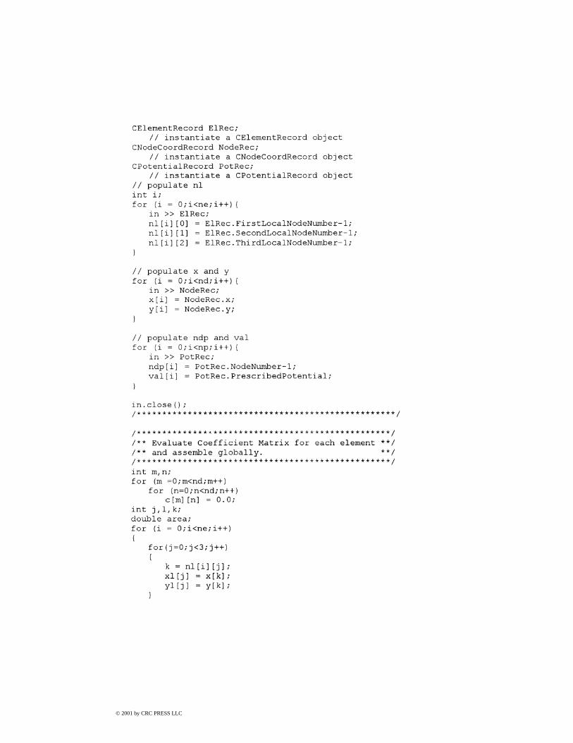
© 2001 by CRC PRESS LLC

© 2001 by CRC PRESS LLC

© 2001 by CRC PRESS LLC

Listing 3: Transmission-line-matrix:
© 2001 by CRC PRESS LLC

© 2001 by CRC PRESS LLC

© 2001 by CRC PRESS LLC

© 2001 by CRC PRESS LLC

© 2001 by CRC PRESS LLC

Listing 4: Fixed-Random Walk Monte Carlo Method:
© 2001 by CRC PRESS LLC

© 2001 by CRC PRESS LLC

Appendix D
Solution of Simultaneous Equations
Application of some numerical methods to EM problems often results in a set ofsimultaneous equations
a11 a12 . . . a1na21 a22 . . . a2n...
...
an1 an2 . . . ann
x1x2...
xn
=
b1b2...
bn
(D.1a)
or
[A][X] = [
B]
(D.1b)
where [A] is the coefficient matrix, [X] is the column matrix of the unknowns to bedetermined, and [B] is the column matrix of constants. Familiarity with the varioustechniques for solving Eq. (D.1) is therefore vital. In this appendix, we provide abrief coverage of direct and iterative procedures for solving Eq. (D.1); direct methodsare more versatile for linear problems, while iterative methods are suitable for non-linear problems. We also consider various techniques for solving eigenvalue systems[A][X] = λ[X].
D.1 Elimination Methods
Elimination methods constitute the simplest direct approach to the solution of aset of simultaneous equations. They usually involve successive elimination of theunknowns by combining equations. Such methods include Gauss’s method, Gauss-Jordan, Cholesky’s or Crout’s method, and the square-root method. Only Gauss’sand Cholesky’s methods will be discussed. The reader should consult [1]–[4] for thetreatment of other methods.
© 2001 by CRC PRESS LLC

D.1.1 Gauss’s Method
This simple method involves eliminating one unknown at a time and proceedingwith the remaining equations. This leads to a set of simultaneous equations in triangu-lar form from which each unknown is determined by back-substitution. To describethis method, consider Eq. (D.1b), i.e.,
a11x1 + a12x2 + · · · + a1nxn = b1 (D.2a)
a21x1 + a22x2 + · · · + a2nxn = b2 (D.2b)
...
an1x1 + an2x2 + · · · + annxn = bn (D.2c)
We divide Eq. (D.2a) by a11 to give
x1 + a′12x2 + · · · + a′
1nxn = b′1 (D.3)
where the primes denote that the coefficients are new. We multiply Eq. (D.3) by −ai1for i = 2, 3, . . . , n and add Eq. (D.3) to the ith equation in (D.2) to eliminate x1 fromother equations so that Eq. (D.2) becomes
x1 + a′12x2 + · · · + a′
1nxn = b′1 (D.4a)
a′22x2 + · · · + a′
2nxn = b′2 (D.4b)
...
a′n2x2 + · · · + a′
nnxn = b′n (D.4c)
Equation (D.2a) used to eliminate x1 from other equations is called the pivot equationand a11 is called the pivot coefficient. We now use Eq. (D.4b) as the pivot equation andwe take similar steps to eliminate x2 from all equations following the pivot equation.Continuing this reduction procedure eventually leads to an equivalent triangular setof equations:
x1 + u12x2 + u13x3 + · · · + u1nxn = c1
x2 + u23x2 + · · · + u2nxn = c2
x3 + · · · + u3nxn = c3 (D.5)...
xn = cn
This completes the first phase known as forward elimination in the Gauss algorithm,and the system in Eq. (D.5) is said to be in upper triangular form. The second phaseknown as back substitution involves solving for the unknowns in Eq. (D.5) by starting
© 2001 by CRC PRESS LLC

at the bottom. That is,
xn = cnxn−1 = cn−1 − un−1,nxn (D.6)
...
x1 = c1 − u12x2 − · · · − u1nxn
In summary, this algorithm can be stated as:
Forward elimination
a′kj = akj /akk, b′
k = bk/akk, j = k, k + 1, . . . , n
a′ij = aij − aika′
kj , i = k + 1, . . . , n (D.7a)
b′i = bi − aikb′
k, i = k + 1, . . . , n
Backward substitution
xn = bn, for the last row
xi = bi −n∑
j=i+1
aij xj , i = n− 1, . . . , 1 (D.7b)
Based on the idea outlined above, a general FORTRAN subroutine for solving aset of simultaneous equations by Gaussian elimination is shown in Fig. D.1.
D.1.2 Cholesky’s Method
This method, also known as Crout’s method or the method of matrix decomposition,involves determining a lower triangular matrix that will reduce the original system inEq. (D.1) to a unit upper triangular matrix. If the original system[
A][X] = [
B]
(D.1a)
or a11 a12 . . . a1na21 a22 . . . a2n...
...
an1 an2 . . . ann
x1x2...
xn
=
b1b2...
bn
(D.1b)
can be redefined in the upper unit triangular matrix [T ] such that[T][X] = [
C]
(D.8a)
© 2001 by CRC PRESS LLC

Figure D.1Gauss elimination method of solving [A][X] = [B].
or
1 T12 . . . T1n0 1 . . . T2n...
...
0 0 . . . 1
x1x2...
xn
=
c1c2...
cn
(D.8b)
the unknown xi can be obtained by back substitution. Let [A] be a product of anupper unit triangular matrix [T ] and a lower triangular matrix [L], i.e.,[
L][T] = [
A]
(D.9)
Since [L][TX − C] = 0 = [
AX − B] , (D.10)
© 2001 by CRC PRESS LLC

it follows that [L][C] = [
B]
(D.11)
For computational reasons, it is convenient to work with the augmented form of thematrices. The augmented matrix is obtained by adding the column vector of constantsto the square coefficient matrix. Equations (D.8) and (D.11) may be combined to give
a11 a12 . . . a1n... b1
a21 a22 . . . a2n... b2
......
an1 an2 . . . ann... bn
=
L11 0 . . . 0L21 L22 . . . 0...
Ln1 Ln2 . . . Lnn
1 T12 . . . T1n... c1
0 1 . . . T2n... c2
...
0 0 . . . 1... cn
(D.12a)
or
[A... B] = [
L][T... C]
(D.12b)
The elements of [L], [T ], and [C] can be defined in terms of [A] and [B] as follows [1,2, 5]:
Lij = aij −j−1∑k=1
LikTkj , i ≥ j, i = 1, 2, . . . , n
Lij = ai1, j = 1
Tij = 1
Lii
(aij −
i−1∑k=1
LikTkj
), i < j, j = 2, 3, . . . , n (D.13)
Tij = aij /a11, i = 1
ci = 1
Lii
(bi −
i−1∑k=1
Likck
), i = 2, 3, . . . , n
c1 = b1/L11
The unknown xi are obtained by back substitution as follows:
xn = cnxi = ci −
n∑j=i+1
Tij xj , i = 1, 2, . . . , n− 1 (D.14)
© 2001 by CRC PRESS LLC

Cholesky’s method can easily be applied in calculating the determinant of [A].Since
det[A] = det
[L]
det[T]
(D.15)
and det[T ] = 1 due to the fact that Tii = 1, it follows that
det[A] = det
[L] = L11L22 . . . Lnn
or
det[A] =
n∏i=1
Lii (D.16)
Figure D.2 shows a subroutine based on Cholesky’s method of solving a set of simul-taneous equations.
D.2 Iterative Methods
The direct or elimination method for solving a system of simultaneous equationscan be used for n = 25 to 60. This number can be greater if the system is wellconditioned or the matrix is sparse. For very large systems, say n = 100 or even1000, elimination methods become time-consuming and prove inadequate due toroundoff error. For these types of problems, indirect or iterative methods provide analternative.
D.2.1 Jacobi’s Method
This is the simplest iterative method. If the system in Eq. (D.1) is rearranged sothat the ith equation is explicit in xi , we obtain
x1 = 1
a11[b1 − a12x2 − a13x3 − · · · − a1nxn] (D.16a)
x2 = 1
a22[b2 − a21x1 − a23x3 − · · · − a2nxn] (D.16b)
...
xn = 1
ann
[bn − an1x1 − an2x2 − · · · − an,n−1xn−1
](D.16c)
assuming that the diagonal elements are all nonzero. We start the solution processby using guesses for the x’s, say x1 = x2 = · · · = xn = 0. The first equation canbe solved for x1, the second for x2, and so on. If we denote the estimates after the
© 2001 by CRC PRESS LLC

Figure D.2Cholesky’s elimination method of solving [A][X] = [B].
© 2001 by CRC PRESS LLC

kth iteration as xk1 , xk2 , . . . , x
kn , the estimates after (k+ 1)th iteration can be obtained
from Eq. (D.16) as
xk+1i = 1
aii
bi − n∑
j=1,j =1
aij xkj
, i = 1, 2, . . . , n (D.17)
The iteration process is continued until values of xi at two successive iterations arewithin an allowable prescribed deviation.
Convergence is measured in terms of the change in xi from the kth iteration to thenext. If we compute
di =∣∣∣∣∣xk+1i − xkixk+1i
∣∣∣∣∣ · 100% (D.18)
for each xi , convergence can be checked using the criterion
di < εs (D.19)
where εs is a specified small quantity. A better test would be to compute
d =
n∑i=1
∣∣∣xk+1i − xki
∣∣∣n∑i=1
∣∣∣xk+1i
∣∣∣· 100% (D.20)
and require that d < εs .
D.2.2 Gauss-Seidel Method
This is the most commonly used iterative method. In Jacobi’s method the entireset of xi from the kth iteration is used in calculating the new set during the (k + 1)thiteration, whereas the most recently calculated value of each variable is used at eachstep in the Gauss-Seidel method. This makes the Gauss-Seidel method convergemore rapidly than (about twice as) Jacobi’s method and is always used in preferenceto it. Instead of Eq. (D.17), we use
xk+1i = 1
aii
bi − i−1∑
j=1
aij xk+1j −
n∑j=i+1
aij xkj
, i = 1, 2, . . . , n (D.21)
A computer program based on this method is displayed in Fig. D.3.
D.2.3 Relaxation Method
This is a slight modification of the Gauss-Seidel method and is designed to enhanceconvergence. If xki is added to the right-hand side of Eq. (D.21) and (aiixki )/aii is
© 2001 by CRC PRESS LLC

Figure D.3Gauss-Seidel iterative method of solving [A][X] = [B].
subtracted from it, we obtain
xk+1i = xki + 1
aii
bi − i−1∑
j=1
aij xk+1j −
n∑j=iaij x
kj
, i = 1, 2, . . . , n (D.22)
The second term on the right-hand side can be regarded as a correction term. Thecorrection term tends to zero as convergence is approached. If this term is multipliedby ω, Eq. (D.22) becomes
xk+1i = xki + ω
aii
bi − i−1∑
j=1
aij xk+1j −
n∑j=iaij x
kj
, i = 1, 2, . . . , n (D.23)
© 2001 by CRC PRESS LLC

The relaxation factor ω is selected such that 1 < ω < 2. The choice of a propervalue ofω is problem dependent and is often determined by trial and error. The addedweight ofω is intended to improve the estimate by pushing it closer to the exact value.
D.2.4 Gradient Methods
The iterative methods considered above may be broadly classified as stationarywhile the ones to be presented now are gradient (or nonstationary) methods. Thetwo common gradient methods are the steepest method and conjugate gradientsmethod [6]–[8]. A major advantage gradient methods have over stationary meth-ods is that convergence is faster; hence gradient methods are particularly useful whenthe number of simultaneous equations is very large.
A set of n simultaneous equations may be solved by finding the position of theminimum of an error function defined over an n-dimensional space. In each step ofa gradient method, a trial set of values for the variables is used to generate a new setcorresponding to a lower value of the error function. If X is the trial vector, the vectorresidual is
R = B − AX (D.24)
where A is real, symmetric, and positive definite. If we define the error function as
e = RtA−1R , (D.25)
then
e = XtAX − 2BtX + BtA−1B (D.26)
showing that e is quadratic in X.Starting from an arbitrary point Xo, we locate a sequence of points
Xk+1 = Xk + αkDk (D.27)
which are successively closer toX, whereXminimizes e in Eq. (D.26). The parameterαk is proportional to the distance betweenXi andXi+1 along the direction vectorDk .Substituting Eq. (D.27) into Eq. (D.26) and setting ∂e/∂αk equal to zero gives
αk = DtkRk
DtkADk(D.28)
Both the methods of steepest descent and conjugate gradients use Eq. (D.28) but differin the choice of Dk .
In the method of descent,Dk is taken as the direction of maximum gradient of e atXk . This direction is proportional to Xk so that the iterative algorithm has the form:
(i) select an arbitrary X0
(ii) compute R0 = B − AX0
© 2001 by CRC PRESS LLC

(iii) determine successively
Uk = ARkαk = RtkRk
RtkUk(D.29)
Xk+1 = Xk + αkRkRk+1 = Rk − αkUk
(iv) repeat step (iii) until residual vector (RT R) becomes sufficiently small.
In the method of conjugate gradients, Dk are selected as n vectors Pk which aremutually conjugate. The vectors Pk are conjugate or orthogonal to A, i.e.,
P tkAPk = 0, i =j=0, i = j (D.30)
Thus the conjugate gradients algorithm is as follows:
(i) select an arbitrary X0
(ii) set P0 = R0 = B − AX0
(iii) determine successively
Uk = ARkαk = P tkRk
P tkUk
Xk+1 = Xk + αkRk (D.31)
Rk+1 = Rk − αkUkβk = −R
tk+1Uk
P tkUk
Pk+1 = Rk + βkPk
(iv) repeat step (iii) until k = n − 1 or the residual vector (RT R) becomes suffi-ciently small.
This algorithm is guaranteed to yield the true solution in no more than n iterations—acondition known as quadratic convergence. Because of this, the conjugate gradientsmethod has the advantage of an iterative scheme in that the roundoff error is limitedonly to the final step of the solution and also the advantage of a direct method in thatit converges to the exact solution in a finite number of steps.
The subroutine in Fig. D.4 applies the conjugate gradients method to solve a givenset of simultaneous equations. Typical areas where the conjugate gradient methodshave been applied in EM can be found in [9]–[12].
© 2001 by CRC PRESS LLC

Figure D.4This subroutine applies the conjugate gradients method to solve [A][X] = [B](Continued).
© 2001 by CRC PRESS LLC

D.3 Matrix Inversion
If [A] is a square matrix, there is another matrix [A]−1, called the inverse of [A],such that [
A][A]−1 = [
A]−1[
A] = [
I]
(D.32)
where I is the identity or unit matrix. Matrix inversion can be used to solve a set ofsimultaneous equations in Eq. (D.1) as
[X] = [
A]−1[
B]
(D.33)
The solution of a system of simultaneous equations by matrix inversion and multi-plication is most valuable when several systems are to be solved, all of which havethe same coefficient matrix but different column matrices of constants. This situationrequires calculating the inverse matrix only once and using it as a premultiplier ofeach of the column matrices of constants [2, 13].
The inversion of matrices is closely related to the solution of sets of simultaneousequations. The inverse of [A] can be determined from Eq. (D.32). If we let [C] =[A]−1, then [
A][C] = [
I]
(D.34a)
or a11 a12 . . . a1na21 a22 . . . a2n...
an1 an2 . . . ann
c11 c12 . . . c1nc21 c22 . . . c2n...
cn1 cn2 . . . cnn
=
1 0 . . . 00 1 . . . 0...
0 0 . . . 1
(D.34b)
This may be regarded as n sets of n simultaneous equations with identical coefficientmatrix. The ith set of n simultaneous equations, for example, is
a11 a12 . . . a1na21 a22 . . . a2n...
ani ani . . . ani...
an1 an2 . . . ann
c1ic2i...
cii...
cni
=
00...
1...
0
(D.35)
Thus, the inversion of [A] may be accomplished by solving n sets of equations likeEq. (D.35). A common approach for matrix inversion is applying elimination method,with or without pivotal compensation. This implies that any elimination technique
© 2001 by CRC PRESS LLC

(Gauss, Gauss-Jordan, or Cholesky’s method) can be modified to calculate an inversematrix. Here we apply the Gauss-Jordan elimination method.
To apply the Gauss-Jordan method, we first augment the coefficient matrix by theidentity matrix to obtain
[A... I] =
a11 a12 . . . a1n... 1 0 . . . 0
a21 a22 . . . a2n... 0 1 . . . 0
.........
an1 an2 . . . ann... 0 0 . . . 1
(D.36)
The goal is to transform this augmented matrix to another augmented matrix of theform
[I... C] =
1 0 . . . 0... c11 c12 . . . c1n
0 1 . . . 0... c21 c22 . . . c2n
.........
0 0 . . . 1... cn1 cn2 . . . cnn
(D.37)
where [C] is the inverse of [A]. The transformation is achieved using the Gauss-Jordanmethod, which involves applying the following equations in the order listed [2]:
a′kj = akj /akk, j = 1, 2, . . . , n, j =ka′kk = 1/akk,
a′ij = aij − aika′
kj , i = 1, 2, . . . , n, i =k (D.38)
j = 1, 2, . . . , n, j =ka′ik = −aika′
kk, i = 1, 2, . . . , n, i =kWe apply Eq. (D.38) for k = 1, 2, . . . , n. A computer program applying Eq. (D.38)is presented in Fig. D.5. An iterative method of correcting the elements of the inversematrix is available in [14].
D.4 Eigenvalue Problems
The nature of these problems is discussed in Section 1.3. Here we are concernedwith the so-called standard eigenproblems
[A− λI ][X] = 0 (D.39)
© 2001 by CRC PRESS LLC

Figure D.5Matrix inversion using Gauss-Jordan elimination method.
or the generalized eigenproblem
[A− λB][X] = 0 (D.40)
To show that Eqs. (D.39) and (D.40) are solved in the same way, we premultiplyEq. (D.40) by B−1 to obtain
[B−1A− λI ][X] = 0 (D.41)
Assuming C = B−1A gives
[C − λI ][X] = 0 (D.42)
© 2001 by CRC PRESS LLC

showing that Eq. (D.39) is a special case of Eq. (D.40) in which B = I . Thus, theprocedure for solving Eq. (D.39) applies to Eq. (D.40) or (D.42).
The eigenvalue problems of Eqs. (D.39) and (D.40) are solved by either direct orindirect methods. In direct methods, such as Jacobi’s method, the relevant matrixelements are stored in the computer, and an explicit procedure is used to obtain someor all of the eigenvalues λ1, λ2, . . . , λn and eigenvalues X1, X2, . . . , Xn. Indirectmethods are basically iterative, and the matrix elements are usually generated ratherthan stored.
D.4.1 Iteration (or Power) Method
The most commonly used iterative method is the power method. The method issuitable in situations where either the greatest or the least eigenvalue is required.Suppose that one of the eigenvalues of A, say λ1, satisfies the condition
|λ1| > |λi | , i =1 , (D.43)
then |λ1| is said to be the dominant eigenvalue of A. In many applications, thedominant eigenvalue is the most important and is probably the only eigenvalue weare interested in. The iteration method is specifically used for finding the dominanteigenvalues.
The iterative procedure is essentially based on the condition that should a trial vector[X]i be assumed, an approximate eigenvalue and a new trial eigenvector [X]i+1 canbe determined from Eq. (D.39) or Eq. (D.40). To find the largest eigenvalue |λ1|, werewrite Eq. (D.39) as
[A][X] = λ[X] (D.44)
and follow these steps [2]:
(1) Assume a trial vector [X]0 = (x1, x2, . . . , xn), e.g., [X]0 = (1, 1, . . . , 1). Sub-stituting [X]0 to the left-hand side of Eq. (D.44) gives the first approximationto the corresponding eigenvector, i.e.,
λ[X]1 = (λx1, λx2, . . . , λxn)
(2) Normalize the new vector λ[X] by dividing it by the magnitude of its first com-ponent or by dividing the vector [X] by the magnitude of the first component.
(3) Substitute the normalized vector into the left-hand side of Eq. (D.44) and obtaina new approximate eigenvector.
(4) Repeat steps (2) and (3) until the components of the new and previous eigen-vectors differ by some prescribed tolerance. The normalizing factor will be thelargest eigenvalue λ1 while [X] is the associated eigenvector.
© 2001 by CRC PRESS LLC

To find the smallest eigenvalue, we first premultiply Eq. (D.44) by the inverse of[A] to obtain
[X] = λ[A]−1[X]or
[A]−1[X] = 1
λ[X] (D.45)
Thus the iteration formula becomes
[A]−1[X]i = 1
λ[X]i+1 (D.46)
In this form, the iteration converges to the largest value 1/λ, which corresponds tothe smallest eigenvalue λ of [A].
Once the largest eigenvalue is found, the method can be used to obtain the nextlargest eigenvalue by transforming [A] to another matrix possessing only the remain-ing eigenvalues [2]. This so-called matrix deflation procedure assumes that [A] issymmetric. The matrix deflation is continued until all the eigenvalues have beenextracted. Error propagation from one stage of the deflation to the next leads to in-accurate results, specially for large eigenproblems. Jacobi’s method, to be discussedin the next section, is recommended for large eigenproblems.
The subroutine in Fig. D.6 is useful for finding the largest eigenvalues of a matrix.
D.4.2 Jacobi’s Method
Jacobi’s method is perhaps the most reliable method for solving eigenvalue prob-lems. Its major advantage is that it finds all eigenvalues and eigenvectors simultane-ously with excellent accuracy.
The method transforms a symmetric matrix [A] into a diagonal matrix having thesame eigenvalues as [A]. This is achieved by eliminating one pair of off-diagonalelements of [A] at a time. Given
[A][X] = λ[X] , (D.47)
let λ1, λ2, . . . , λn be the eigenvalues and [V1], [V2], . . . , [Vn] the correspondingeigenvectors. Then, [
A][V1] = λ1
[V1][
A][V2] = λ2
[V2]
...[A][Vn] = λ1
[Vn]
(D.48)
or simply
[A][V ] = [V ][λ] (D.49)
© 2001 by CRC PRESS LLC

Figure D.6Subroutine for finding the largest eigenvalue of equation [A][X] = LAMBDA[X](Continued).
© 2001 by CRC PRESS LLC

Figure D.6(Cont.) Subroutine for finding the largest eigenvalue of equation [A][X] =LAMBDA[X].
where
[V ] = [[V1],[V2], . . . ,
[Vn]]
(D.50a)
[λ] =
λ1 0 . . . 00 λ2 . . . 0......
...
0 0 . . . λn
(D.50b)
From the theory of matrices, if [A] is symmetric, [V ] is orthogonal, i.e.,
[V ]t = [V ]−1 (D.51)
hence, premultiplying Eq. (D.49) by [V ]t leads to
[V ]t [A][V ] = [λ] (D.52)
signifying that the eigenvalues of [V ]t [A][V ], which is known as the orthogonaltransformation of [A], are the same as those of [A]. Thus the problem of finding theeigenvalues is reduced to finding the [V ] matrix.
The [V ] matrix is constructed iteratively by using unitary matrix (or plane rotationmatrix) [R]. If we let[
A1] = [
A]
[A2] = [
R1]t [A1][R1]
[A3] = [
R2]t [A2][R2] = [
R2]t [R1]t [A][R1][R2]
...[Ak] = [
Rk−1]t. . .[R1]t [A][R1]. . .[Rk−1
], (D.53)
then as k → ∞ [Ak] → [
λ][
R1][R2]. . .[Rk−1
] → [V]
(D.54)
© 2001 by CRC PRESS LLC

The unitary transformation matrix [R] eliminates the pair of equal elements apq andaqp. It is given by [1, 2, 7]
p q
[Rk] =
11
cos θ − sin θ1
sin θ cos θ1
p
q
(D.55a)
i.e.,
Rqq = Rpp = cos θ
−Rpq = Rqp = sin θ
Rii = 1, i =p, qRij = 0, elsewhere (D.55b)
The choice of θ in the transformation matrix must be such that new elements a′pq =
a′qp = 0, i.e.,
a′pq = (−app + aqq
)cos θ sin θ + apq
(cos2 θ − sin2 θ
)= 0 (D.56)
Hence
tan 2θ = 2apqapp − aqq , −45◦ < θ < 45◦ (D.57)
An alternative manipulation of Eq. (D.56) gives
cos θ =√(app − aqq)2 + 4a2
pq + (app − aqq)2√(app − aqq)2 + 4a2
pq
1/2
(D.58a)
sin θ = apq√(app − aqq)2 + 4a2
pq cos θ(D.58b)
Notice that Eq. (D.53) requires an infinite number of transformations because theelimination of elements apq and aqp in one step will in general undo the elimination ofpreviously treated elements in the same row or column. However, the transformationconverges rapidly and ceases when all the off-diagonal elements become negligiblein magnitude.
The program in Fig. D.7 determines all the eigenvalues and eigenvectors of sym-metric matrices employing Jacobi’s method.
© 2001 by CRC PRESS LLC

Figure D.7Subroutine for finding all the eigenvalues and eigenvectors of equation [A][X] =LAMBDA[x] (Continued.)
© 2001 by CRC PRESS LLC

Figure D.7(Cont.) Subroutine for finding all the eigenvalues and eigenvectors of equation[A][X] = LAMBDA[x].
© 2001 by CRC PRESS LLC

References
[1] A.W. Al-Khafaji and J.R. Tooley, Numerical Methods in Engineering Practice.New York: Rinehart and Winston, 1986, pp. 84–159, 203–270.
[2] M.L. James et al., Applied Numerical Methods for Digital Computation. 3rded., New York: Harper & Row, 1985, pp. 146–298.
[3] S.A. Hovanessian and L.A. Pipes, Digital Computer Methods in Engineering.New York: McGraw-Hill, 1969, pp. 1–48.
[4] W. Cheney and D. Kincaid, Numerical Mathematics and Computing, 2nd ed.,Monterey, CA: Brooks/Cole, 1985, pp. 201–257.
[5] R.L. Ketter and S.P. Prawel, Modern Methods of Engineering Computation.New York: MacGraw-Hill, 1969, pp. 66–117.
[6] A. Ralston and H.S. Wilf (eds.), Mathematical Methods for Digital Computers.New York: John Wiley, 1960, pp. 62–72.
[7] A. Jennings, Matrix Computation for Engineers and Scientists. New York: JohnWiley, 1977, pp. 182–222, 250–254.
[8] J.C. Nash, Compact Numerical Methods for Computers: Linear Algebra andFunction Minimization. New York: John Wiley, 1979, pp. 195–199.
[9] T.K. Sarkar, et al., “A limited survey of various conjugate gradient methods forsolving complex matrix equations arising in electromagnetic wave interaction,”Wave Motion, vol. 10, no. 6, 1988, pp. 527–546.
[10] A.F. Peterson and R. Mittra, “Method of conjugate gradients for the numericalsolution of large-body electromagnetic scattering problems,” J. Opt. Soc. Am.,Pt. A, vol. 2, no. 6, June 1985, pp. 971–977.
[11] T.K. Sarkar, “Application of the Fast Fourier transform and the conjugate gradi-ent method for efficient solution of electromagnetic scattering from both elec-trically large and small conducting bodies,” Electromagnetics, vol. 5, 1985,pp. 99–122.
[12] D.T. Borup and O.P. Gandhi, “Calculation of high-resolution SAR distributionsin biological bodies using the FFT algorithm and conjugate gradient method,”IEEE Trans. Micro. Theo. Tech., vol. MTT-33, no. 5, May 1985, pp. 417–419.
[13] R.W. Southworth and S.L. Deleeuw, Digital Computation and Numerical Meth-ods. New York: MacGraw-Hill, 1965, pp. 247–251.
[14] S. Hovanessian, Computational Mathematics in Engineering. Lexington, MA:Lexington Books, 1976, p. 25.
© 2001 by CRC PRESS LLC

Appendix E
Answers to Odd-Numbered Problems
Chapter 1
1.1 Proof.
1.3 Proof.
1.5 They satisfy Maxwell’s equations.
1.7 Es = 1
jωεo
Ho√ρ
(1
ρ2− jβ
)e−jβρaz.
1.9 Hs = −j 20
ωµo
[ky sin(kxx) sin(kyy)ax + kx cos(kxx) cos(kyy)ay
].
1.11 (a) cos(ωt − 2z)ax − sin(ωt − 2z)ay
(b) −10 sin x sinωtax − 5 cos(ωt − 2z+ 45◦)az(c) 2 cos 2x cos(ωt − 3x − 90◦)+ e3x cos(ωt − 4x).
1.13 Proof.
1.15 (a) elliptic, (b) elliptic, (c) hyperbolic, (d) parabolic.
Chapter 2
2.1 If a and d are functions of x only; c and e are functions of y only; b = 0; andf is the sum of a function x only and a function of y only.
2.3 (a) V =∞∑n=1
An sin(nπaa
)sinh
[nπa(y − a)
], where
© 2001 by CRC PRESS LLC

An = 2
n sinh
(−nπb
a
) ∫ a
0
Vox
asin
nπx
adx
(b) V = Vo
cosπx
acosh
πy
a
coshπb
a
.
2.5 (a) �(ρ, φ) = sin φ
ρ
(b) �(ρ, z) = 4
π
∞∑n=1,3,5
I0(nπρ/L)
I0(nπa/L)
sin(nπz/L)
n
(c) �(ρ, φ, t) = 2∞∑n=1
J2(ρxn/a)
xnJ3(xn)cos 2φ exp
[−x2
nkt/a2],
where J2(xn) = 0.
2.7 V (ρ, z) =∞∑n=1
An sin(nπzL
)I0
(nπρL
), 0.2639Vo.
2.9 V (ρ, φ) = 4Voπ
∞∑n=1,3,5
1
n
[(ρa
)3n −(ρa
)−3n]
[(b
a
)3n
−(b
a
)−3n] sin 3nφ.
2.11 Proof.
2.13 Proof.
2.15a
(ρ2 + a2)3/2,
a2 − ρ2
(ρ2 + a2)5/2.
2.17 (a) 0, (b)2
9, (c)
1
24.
2.19 (a)1
2+
∞∑n=1
(2n+ 1)
2n(n+ 1)P 1n (0)(r/a)
nPn(cos θ)
(b) −7
5
a3
r2P1(cos θ)− 3
10
a5
r4P3(cos θ).
2.21 For r < a, 0 ≤ θ ≤ π/2,
V = aρ
2ε
[−z+
∞∑n=0
(−1)n(2n)!(n!2n)2 (r/a)2nP2n(cos θ)
]
For r > a, V = aρ
2ε
[ ∞∑n=0
(−1)n+1(2n+ 2)![(n+ 1)!2n+1]2
(r/a)2n+1P2n(cos θ)
].
© 2001 by CRC PRESS LLC

2.23 Proof.
2.25 V (r, θ) = 2(r/a)2P2(cos θ)+ 3r
aP1(cos θ)+ 2P0(cos θ).
2.27 For r < a, V (r, θ) = − 3Eoεr + 2
cos θ
For r > a, V (r, θ) = −Eor cos θ + Eoa3(εr − 1)
r2(εr + 2)cos θ .
2.291
3cos 2φP 2
2 (cos θ).
2.31 (a)32
π3
∞∑m=1
∞∑n=1
∞∑p=1
m[1 − (−1)meπ ](m2 + 1)(2n− 1)(2p − 1)
· sinmx sin(2n− l)y sin(2p − l)z
[m2 + (2n− 1)2 + (2p − 1)2]
(b) −128
π3
∞∑m=1
∞∑n=1
∞∑p=1
1
(2m− 3)(3m2 − 1)(2n− 1)(2p − 1)
· sin(2m− 1)x sin(2n− l)y sin(2p − l)z
[(2m− 1)2 + (2n− 1)2 + (2p − 1)2] .
2.33 V (x, y) =∞∑m=1
∞∑n=1
2ρo cosmπ(cos nπ − 1)
π2mnε[(mπ/a)2 + (nπ/b)2] sin(mπx/a) sin(nπy/b).
2.35
V =
∞∑k=1
sin βx[an sinh βy + bn cosh βy], 0 ≤ y ≤ c
∞∑k=1
cn sin βx sinh βy, c ≤ y ≤ b
where β = nπ
a, n = 2k − 1.
2.37 P 01 = 0.5, P 0
2 = −1.250, P 12 = 1.29904, P 2
3 = 2.25, P 03 = −0.4375, P 1
3 =0.32476, P 2
3 = 5.625, P 33 = 9.74279, etc.
2.39 Derivation/Proof.
2.41 Proof.
2.43 Proof.
2.47 See Fig. E.1.
2.49 See Fig. E.2.
© 2001 by CRC PRESS LLC

Figure E.1For Problem 2.47.
Figure E.2For Problem 2.49.
© 2001 by CRC PRESS LLC

Chapter 3
3.1 Proof.
3.3 (1 − a2)[�(i + 1, j + 1) + �(i − 1, j − 1)] − 2[�(i, j + 1) + �(i, j − 1)−a2�(i+ 1, j)−a2�(i− 1, j)]+�(i− 1, j + 1)+�(i− 1, j − 1)−�(i+1, j − 1)−�(i − 1, j − 1) = 0.
3.5 Proof.
3.7 VA = 61.46 = VE, VB = 21.95 = VD, VC = 45.99V .
3.9 16.67V .
3.11 r ≤ 1/2.
3.13 (a) Proof, (b) Proof, (c) Euler: r ≤ 1/4 for stability, Leapfrog: unstable,Dufort-Frankel: unconditionally stable.
3.15 (a) After 5 iterations, V1 = 73.79, V2 = 79.54, V3 = 40.63, V4 = 45.31,V5 = 61.33
(b) After 5 iterations, V1 = 19.93, V2 = 19.96, V3 = 6.634, V4 = 6.649.
3.19 (a) 60.51 0, (b) 50.44 0.
3.21 kc = 4.443 (exact), kc = 3.5124 (exact).
3.23 Proof.
3.25 See Fig. E.3.
3.27 68.85, 23.32, 6.4, 10.23, 10.34.
3.29 Proof.
3.31
µo∂Hxy
∂t+ σ ∗
y Hxy = − ∂
∂y
(Ezx + Ezy
)µo∂Hxz
∂t+ σ ∗
y Hxz = ∂
∂z
(Eyx + Eyz
)...
εo∂
∂tEzx + σxEzx = ∂
∂x
(Hyx + Eyz
)εo∂
∂tEzy + σyEzy = − ∂
∂y
(Hxy + Exz
).
© 2001 by CRC PRESS LLC

Figure E.3For Problem 3.25.
3.33 Proof.
3.35 (a) 0.9047, (b) 0.05324.
3.37 1.218.
3.43 (a) 1.724, (b) 3.963, (c) 15.02.
Chapter 4
4.1 (a) 1.3333, (b) −4.667, (c) 157.08.
4.3 (a) y′′ = 0, (b) 1 + y′2 − yy′′ = 0,
(c) xy′ cos(xy′)+ sin(xy′) = 0, (d) y′′ + y = 0,
(e) 2yiv − 10y = 0, (f) 3u+ 2v′′ = 0.
4.5 Proof.
4.7 Proof.
4.9 ρv = ∇ · D.
4.11 I = 1
2
∫v
[εx
(∂V
∂x
)2
+ εy
(∂V
∂y
)2
+ εz
(∂V
∂z
)2
− 2ρvV
]dv.
© 2001 by CRC PRESS LLC

4.131
2
∫ [(y′)2 + y2 − 2y sin πx
]dx
4.15 For exact, � = 2.1667x − 0.1667x3,
for N = 1, � = 2.25x − 0.25x2
for N = 2, 3, � is the same as the exact solution.
4.17 (a) a1 = 10.33, a2 = −1.46, a3 = 0.48
(b) a1 = 10.44, a2 = −1.61, a3 = 0.67
(c) a1 = 10.21, a2 = −1.32, a3 = 0.35
(d) a1 = 10.21, a2 = −1.32, a3 = 0.35
4.19 See table below.
Method a1 a2Collocation 0.9292 −0.05115Subdomain 0.9237 −0.05991Galerkin 0.9334 −0.05433Least squares 0.9327 −0.06813Rayleigh–Ritz 0.09334 −0.05433
4.21 � = (1 − x)(1 − 0.2090x − 0.789x2 + 0.2090x3).
4.23 λ = 0.2, λo = 0.1969 (exact).
4.25 a/λc = 0.2948.
Chapter 5
5.1 (a) Nonsingular, Fredholm IE of the 2nd kind,
(b) nonsingular, Volterra IE of the 2nd kind,
(c) nonsingular, Fredholm IE of the 2nd kind.
5.3 (a) y = x −∫ x
0(x − t)y dt
(b) y = 1 + x − cos x −∫ x
0(x − t)y(t) dt
5.5 Proof.
© 2001 by CRC PRESS LLC

5.7
G(x, y; x′, y′) = − 4
abex
′−x∞∑m=1
∞∑n=1
sinmπx
asin
mπy
bsin
mπx′
asin
mπy′
b
1 + (mπ/a)2 + (nπ/b)2
5.11 Proof.
5.13 Proof.
5.15 (a) 62.71 0, (b) 26.75 0.
5.21 (a) Proof, (b) See Fig. E.4(a), (c) See Fig. E.4(b).
5.23 (a) See Fig. E.5(a), (b) See Fig. E.5(b).
5.25 The distribution of normalized field, |Ex |/|Ei |, is shown in Fig. E.6.
5.27 See table below.
Cell En
64 0.134265 0.396666 0.429267 0.174974 0.096575 0.392576 0.417377 0.139384 0.134285 0.396686 0.429387 0.1749
Chapter 6
6.1 (a)
0.5909 −0.1364 −0.4545−0.1364 0.4545 −0.3182−0.4545 −0.3182 0.7727
(b)
0.6667 −0.6667 0−0.6667 1.042 −0.375
0 −0.375 0.375
© 2001 by CRC PRESS LLC

Figure E.4(a) For Problem 5.21.
Figure E.4(b) For Problem 5.21.
6.3 α1 = 1
23[4x + 3y − 24], α2 = 1
23[−5x + 2y + 30], α3 = 1
23[x − 5y + 17].
6.51
2ε [V1 V2 V3]
hyV1
2hx− hyV2
2hx
−hyV1
2hx+ V2(h
2x + h2
y)
2hxhy− V3hx
2hy
−hxV2
2hy+ hxV3
2hy
© 2001 by CRC PRESS LLC

Figure E.5(a) For Problem 5.23.
Figure E.5(b) For Problem 5.23.
© 2001 by CRC PRESS LLC

Figure E.6For Problem 5.25.
6.9 Calculate E using
E = − 1
2A
3∑i=1
PiVeiax − 1
2A
3∑i=1
QiVeiay
6.11 See Fig. E.7.
6.13 λc,mn = a
2
√(m+ n)2 + n2, a = 1.
6.17 B = 14. See the mesh in Fig. E.8, B = 4.
6.19 Proof.
© 2001 by CRC PRESS LLC

Figure E.7For Problem 6.11.
Figure E.8For Problem 6.17.
6.21 (a)32A
180, (b) − A
45, (c) 0.
6.23A
180
6 0 0 − 1 4 −10 32 16 0 16 −40 16 32 −4 16 0
−1 0 −4 6 0 −1−4 16 16 0 32 0−1 −4 0 −10 6
6.25
D(1) =1 1 1
0 0 00 0 0
, D(2) =0 0 1
1 1 10 0 0
, D(3) =0 0 0
0 0 01 1 1
© 2001 by CRC PRESS LLC

D(1) =
3 1 1 −1 −1 −10 2 0 4 2 00 0 2 0 2 40 0 0 0 0 00 0 0 0 0 00 0 0 0 0 0
D(2) =
0 0 0 0 0 04 2 0 0 0 00 0 0 0 0 0
−1 1 −1 3 1 −10 0 2 0 2 40 0 0 0 0 0
D(3) =
0 0 0 0 0 00 0 0 0 0 04 2 2 0 0 00 0 0 0 0 00 2 0 4 2 0
−1 −1 1 −1 1 3
6.27 Proof.
6.29v
20
2 1 1 11 2 1 11 1 2 11 1 1 2
6.31 B1 = ∂
∂ρ+ jk + 1
2ρ
B2 = ∂
∂ρ+ jk + 1
2ρ− 1
8ρ(1 + jkρ)− 1
2ρ(1 + jkρ)
∂2
∂φ2.
Chapter 7
7.1 Proof.
7.3 Proof.
7.5 ;</λ = 0.0501.
7.7 See Fig. E.9.
7.9 Proof.
© 2001 by CRC PRESS LLC

Figure E.9For Problem 7.7.
7.11 Proof.
7.131
6ns.
7.15 See Table below.
|Z| Arg(Z);</λ TLM Exact TLM Exact
0.023 4.1981 6.1272 −0.2806 −0.01060.025 2.382 2.4898 1.2546 1.06100.027 0.3281 0.3252 −0.7952 −0.85540.029 5.2724 5.1637 0.8459 0.86780.031 0.2963 0.3039 −1.1340 −1.16100.033 1.8117 1.8038 1.3408 1.33850.035 0.8505 0.8529 −1.3820 −1.40250.037 0.4912 0.4838 1.3914 1.39320.039 5.3772 5.4883 −1.1022 −1.11550.041 0.2115 0.2179 −1.2795 −1.3174
7.17 For εr = 2, kca = 1.303; for εr = 8, kca = 0.968.
7.19 See Fig. E.10.
© 2001 by CRC PRESS LLC

Figure E.10For Problem 7.19.
Chapter 8
8.3 (a) 16, 187, 170, 429, 836, 47, 950, 369, 456, 307
(b) 997, 281, 13, 449, 277, 721, 133, 209, 757, 761.
8.7 M = 5, a = 0, b = 1. Generate the random variable as follows:
(1) Generate two uniformly distributed random variables U1 and U2 from(0, 1).
(2) Check if U2 ≤ fX(U2)/M = U2.
(3) If the inequality holds, accept U2.
(4) Otherwise, reject U1 and U2 and repeat (1) to (3).
8.9 (a) 3.14159 (exact), (b) 0.4597 (exact), (c) 1.71828 (exact), (d) 2.0.
8.11 0.4053 (exact).
8.13 2.5 (exact).
8.15 V (0.4, 0.2) = 1.1, V (0.35, 0.2) = 1.005, V (0.4, 0.15) = 1.05, V (0.45, 0.2) =1.15, V (0.4, 0.25) = 1.15.
8.17 2.991V .
© 2001 by CRC PRESS LLC

8.19 1.2 V .
8.21 V (2, 10) = 65.85, V (5, 10) = 23.32, V (8, 10) = 6.4, V (5, 2) = 10.23,V (5, 18) = 10.34.
8.23 (a) 0.33, 0.17, 0.17, 0.33,
(b) 0.455, 0.045, 0.045, 0.455.
8.25 12.11 V .
8.27 10.44 V .
8.29 25.0 V .
8.31 See Table below.
Node Markov Exodus Finite(ρ, z) chain method difference
(5, 18) 11.39 11.44 11.47(5, 10) 27.47 27.82 27.87(5, 2) 12.31 12.18 12.13(10, 2) 2.448 2.352 2.342(15, 2) 0.4684 0.3842 0.3965
Chapter 9
9.1 Proof.
9.3 Tij =√
2
N + 1/2cos
(i − 0.5)(j − 0.5)π
N + 0.5
λk = 2 sin
(k − 0.5
N + 0.5
)π
9.9 Proof.
© 2001 by CRC PRESS LLC


![[Solutions Manual] Elements of Electromagnetics - Sadiku - 3rd.pdf](https://static.documents.pub/doc/80x56/55cf9d4f550346d033ad120e/solutions-manual-elements-of-electromagnetics-sadiku-3rdpdf.jpg)


![[Solutions manual] elements of electromagnetics BY sadiku - 3rd](https://static.documents.pub/doc/80x56/55c355babb61eb0a7e8b459d/solutions-manual-elements-of-electromagnetics-by-sadiku-3rd.jpg)


![[Oficial] solution book elements of electromagnetic 3ed sadiku](https://static.documents.pub/doc/80x56/55a693eb1a28ab4a4d8b47f5/oficial-solution-book-elements-of-electromagnetic-3ed-sadiku.jpg)
