Initial Algebras of Terms,with binding and algebraic structure

Bart Jacobs1 and Alexandra Silva1

Institute for Computing and Information Sciences, Radboud University Nijmegen{bart,alexandra}@cs.ru.nl

July 15, 2013

Abstract. One of the many results which makes Joachim Lambek famous is:an initial algebra of an endofunctor is an isomorphism. This fixed point result isoften referred to as “Lambek’s Lemma”. In this paper, we illustrate the power ofinitiality by exploiting it in categories of algebra-valued presheaves EM(T )N, fora monad T on Sets. The use of presheaves to obtain certain calculi of expressions(with variable binding) was introduced by Fiore, Plotkin, and Turi. They used set-valued presheaves, whereas here the presheaves take values in a category EM(T )of Eilenberg-Moore algebras. This generalisation allows us to develop a theorywhere more structured calculi can be obtained. The use of algebras means alsothat we work in a linear context and need a separate operation ! for replication, forinstance to describe strength for an endofunctor on EM(T ). We apply the resultingtheory to give systematic descriptions of non-trivial calculi: we introduce non-deterministic and weighted lambda terms and expressions for automata as initialalgebras, and we formalise relevant equations diagrammatically.

1 Introduction

In [22] Joachim Lambek proved a basic result that is now known as “Lambek’s Lemma”.It says: an initial algebra F(A) → A of an endofunctor F : C → C is an isomorphism.The proof is an elegant, elementary exercise in diagrammatic reasoning. The functor Fcan be seen as an abstraction of a signature, describing the arities of operations. Theinitial algebra, if it exists, is then the algebra whose carrier is constructed inductively,using these operations for the formation of terms. This “initial algebra semantics” formsthe basis of the modern perspective on expressions (terms, formulas) defined by opera-tions, in logic and in computer science. An early reference is [11]. A map going out ofan initial algebra, obtained by initiality, provides denotational semantics of expressions.By construction this semantics is “compositional”, which is a way of saying that it is ahomomorphism of algebras.

A more recent development is to use the dual approach, involving coalgebras X →G(X), see [28,17]; they capture the operational semantics of languages, describing thebehaviour in terms of elementary steps. By duality, Lambek’s Lemma also applies inthis setting: a final coalgebra is an isomorphism. One of the highlights of the categor-ical approach to language semantics is the combined description of both denotationaland operational semantics in terms of algebras and coalgebras of a functors (typicallyconnected via distributive laws, see [19] for an overview).

This paper contains the first part of a study elaborating such a combined approach,using algebra-valued presheaves. It concentrates on obtaining structured terms as ini-tial algebras. Historically, the first examples of initial algebras appeared in the categorySets, of sets and functions. But soon it became clear that initiality (or finality) in morecomplicated categories gives rise to a richer theory, involving additional language struc-ture or stronger initiality principles.

– Induction with parameters (also called recursion) can be captured via initiality in“simple” slice categories, see e.g. [14]; similarly, initiality in (ordinary) slice cate-gories gives a dependent form of induction, see [1].

– Expressions with variable binding operations like λx. xx in the lambda calculus canbe described via initiality in presheaf categories, as shown in [8].

– This approach is extended to more complicated expressions, like in the π-calculusprocess language, see [10,9].

– The basics of Zermelo-Fraenkel set theory can be developed in a category with asuitably rich collection of map, see [18].

– Final coalgebras in Kleisli categories of a monad give rise to so-called trace seman-tics, see [12].

This paper contains an extension of the second point: the theory developed in [8] usesset-valued presheaves N → Sets. In contrast, here we use algebra-valued presheavesN → EM(T ), where EM(T ) is the category of Eilenberg-Moore algebras of a monadT on Sets. The concrete examples elaborated at the end of the paper involve (1) thefinite power set monad Pfin, with algebras EM(Pfin) = JSL, the category of join semi-lattices, and (2) the multiset monad MS for a semiring S , with semimodules over S asalgebras. The initial algebras in the category of presheaves over these Eilenberg-Moorecategories have non-determinism and resource-sensitivity built into the languages, seeSection 5. Moreover, in the current framework we can diagrammatically express rele-vant identifications, like the (β)-rule for the lambda calculus and the “trace equation” ofRabinovich [27].

The use of a category of algebras EM(T ) instead of Sets requires a bit more care.The first part of the paper is devoted to extending the theory developed in [8] to this al-gebraic setting. The most important innovation that we need is the replication operation!, known from linear logic. Since Eilenberg-Moore categories are typically linear —with tensors ⊗ instead of cartesian products ×— we have to use replication ! explicitlyif we need non-linear features. For instance, substitution t[s/v], that is, replacing alloccurrences of the variable v in t by a term s, may require that we use s multiple times,namely if the variable v occurs multiple times in t. Hence the type of s must be !Terms,involving explicit replication !.

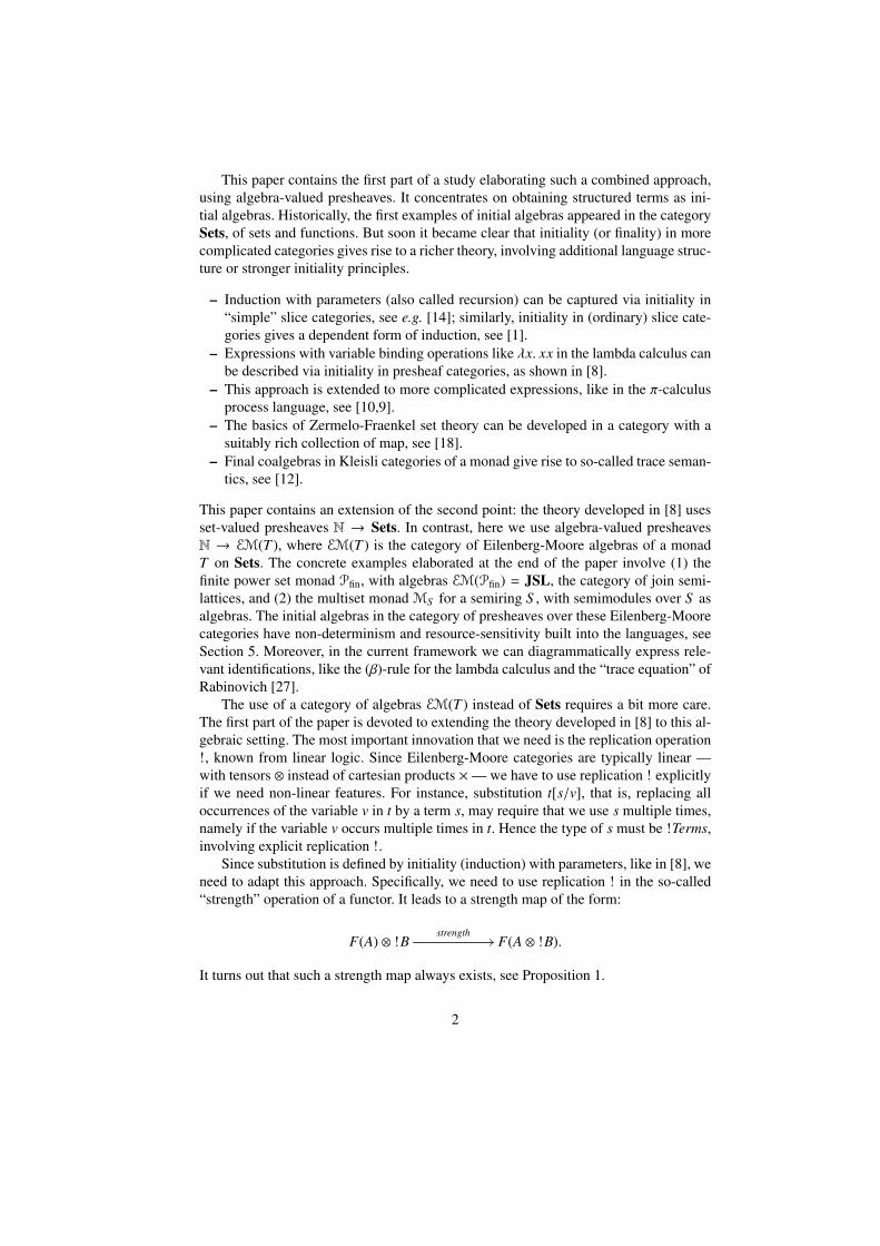
Since substitution is defined by initiality (induction) with parameters, like in [8], weneed to adapt this approach. Specifically, we need to use replication ! in the so-called“strength” operation of a functor. It leads to a strength map of the form:

F(A) ⊗ !Bstrength

// F(A ⊗ !B).

It turns out that such a strength map always exists, see Proposition 1.

2

In the end, in Section 5, we show how an initial algebra — of an endofunctor onsuch a rich universe as given by algebra-valued presheaves — gives rise to a very richlanguage in which many features are built-in and provided implicitly by the categoricalinfrastructure. This forms an illustration of the desirable situation where the formalismdoes the work for you. It shows the strength of the concepts that Joachim Lambekalready worked on, almost fifty years ago.

2 Monads and their Eilenberg-Moore categories

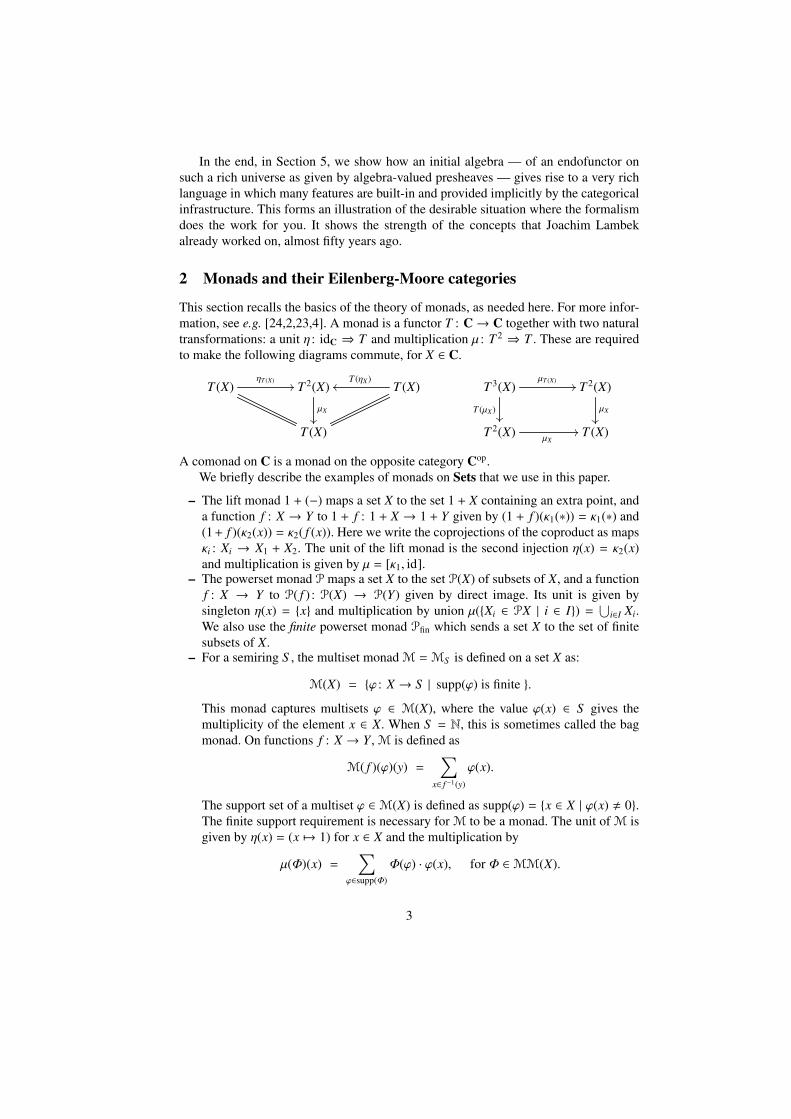
This section recalls the basics of the theory of monads, as needed here. For more infor-mation, see e.g. [24,2,23,4]. A monad is a functor T : C→ C together with two naturaltransformations: a unit η : idC ⇒ T and multiplication µ : T 2 ⇒ T . These are requiredto make the following diagrams commute, for X ∈ C.

T (X)ηT (X)

// T 2(X)

µX

��

T (X)T (ηX )

oo T 3(X)µT (X)

//

T (µX )��

T 2(X)

µX

��

T (X) T 2(X)µX

// T (X)

A comonad on C is a monad on the opposite category Cop.We briefly describe the examples of monads on Sets that we use in this paper.

– The lift monad 1 + (−) maps a set X to the set 1 + X containing an extra point, anda function f : X → Y to 1 + f : 1 + X → 1 + Y given by (1 + f )(κ1(∗)) = κ1(∗) and(1+ f )(κ2(x)) = κ2( f (x)). Here we write the coprojections of the coproduct as mapsκi : Xi → X1 + X2. The unit of the lift monad is the second injection η(x) = κ2(x)and multiplication is given by µ = [κ1, id].

– The powerset monad P maps a set X to the set P(X) of subsets of X, and a functionf : X → Y to P( f ) : P(X) → P(Y) given by direct image. Its unit is given bysingleton η(x) = {x} and multiplication by union µ({Xi ∈ PX | i ∈ I}) =

⋃i∈I Xi.

We also use the finite powerset monad Pfin which sends a set X to the set of finitesubsets of X.

– For a semiring S , the multiset monad M =MS is defined on a set X as:

M(X) = {ϕ : X → S | supp(ϕ) is finite }.

This monad captures multisets ϕ ∈ M(X), where the value ϕ(x) ∈ S gives themultiplicity of the element x ∈ X. When S = N, this is sometimes called the bagmonad. On functions f : X → Y , M is defined as

M( f )(ϕ)(y) =∑

x∈ f −1(y)

ϕ(x).

The support set of a multiset ϕ ∈M(X) is defined as supp(ϕ) = {x ∈ X | ϕ(x) , 0}.The finite support requirement is necessary for M to be a monad. The unit of M isgiven by η(x) = (x 7→ 1) for x ∈ X and the multiplication by

µ(Φ)(x) =∑

ϕ∈supp(Φ)

Φ(ϕ) · ϕ(x), for Φ ∈MM(X).

3

Here, and later in the examples, we use the notation (x 7→ s) to denote a functionϕ : X → S assigning s to x and 0 to all other x′ ∈ X.

For an arbitrary monad T = (T, η, µ) we write EM(T ) for the category of Eilenberg-Moore algebras. Its objects are maps of the form α : T (X) → X satisfying α ◦ η = idand α ◦ µ = α ◦ T (α). A homomorphism

(α : T (X) → X

)−→

(β : T (Y) → Y

)in

EM(T ) is a map f : X → Y between the underlying objects satisfying f ◦ α = β ◦ T ( f ).This yields a category, with obvious forgetful functor U : EM(T ) → Sets. This functorU has a left adjoint F, mapping an object X to the free algebra F(X) =

(µ : T 2(X) →

T (X))

on X.A category of algebras inherits all limits from the underlying category. In the special

case of a monad T on Sets, all colimits also exist in EM(T ), by a result of Linton, see [2,§9.3, Prop. 4]. This category EM(T ) is also symmetric monoidal closed, provided themonad T is commutative (i.e. monoidal), see [21,20]. We write the tensors as ⊗, withtensor unit I, and exponential (. The free functor F : Sets → EM(T ) preserves themonoidal structure: F(X × Y) � F(X) ⊗ F(Y) and F(1) � I, where 1 is a singleton set.As a result the set A ( B, for A, B ∈ EM(T ), contains the homomorphisms A → B inEM(T ).

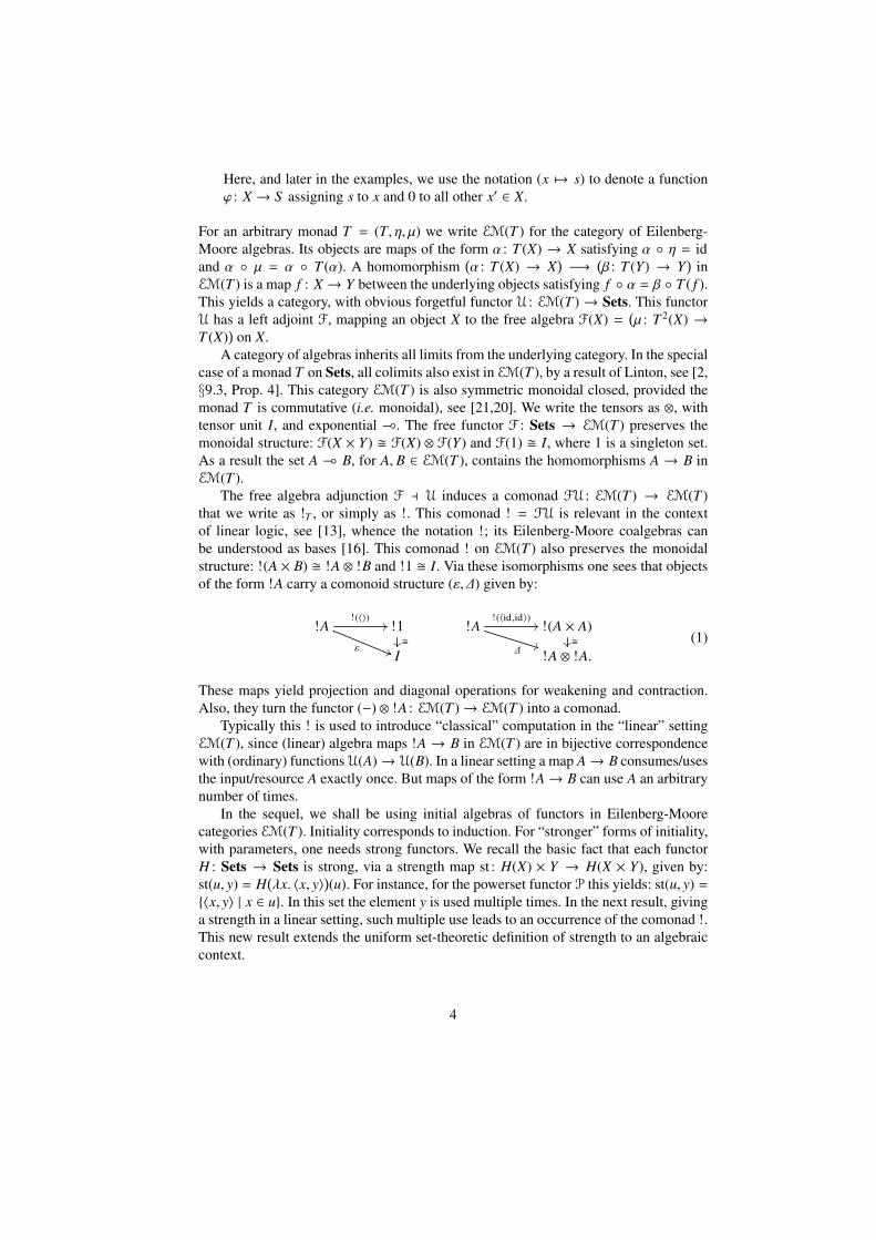
The free algebra adjunction F a U induces a comonad FU : EM(T ) → EM(T )that we write as !T , or simply as !. This comonad ! = FU is relevant in the contextof linear logic, see [13], whence the notation !; its Eilenberg-Moore coalgebras canbe understood as bases [16]. This comonad ! on EM(T ) also preserves the monoidalstructure: !(A × B) � !A ⊗ !B and !1 � I. Via these isomorphisms one sees that objectsof the form !A carry a comonoid structure (ε, ∆) given by:

!A!(〈〉)

//

ε ))

!1���

!A!(〈id,id〉)

//

∆**

!(A × A)���

I !A ⊗ !A.(1)

These maps yield projection and diagonal operations for weakening and contraction.Also, they turn the functor (−) ⊗ !A : EM(T )→ EM(T ) into a comonad.

Typically this ! is used to introduce “classical” computation in the “linear” settingEM(T ), since (linear) algebra maps !A → B in EM(T ) are in bijective correspondencewith (ordinary) functions U(A)→ U(B). In a linear setting a map A→ B consumes/usesthe input/resource A exactly once. But maps of the form !A→ B can use A an arbitrarynumber of times.

In the sequel, we shall be using initial algebras of functors in Eilenberg-Moorecategories EM(T ). Initiality corresponds to induction. For “stronger” forms of initiality,with parameters, one needs strong functors. We recall the basic fact that each functorH : Sets → Sets is strong, via a strength map st : H(X) × Y → H(X × Y), given by:st(u, y) = H

(λx. 〈x, y〉

)(u). For instance, for the powerset functor P this yields: st(u, y) =

{〈x, y〉 | x ∈ u}. In this set the element y is used multiple times. In the next result, givinga strength in a linear setting, such multiple use leads to an occurrence of the comonad !.This new result extends the uniform set-theoretic definition of strength to an algebraiccontext.

4

Proposition 1. Let T be a commutative monad on Sets, and H : EM(T ) → EM(T ) bean arbitrary functor. For algebras A, B there is a “non-linear” strength map:

H(A) ⊗ !B st // H(A ⊗ !B). (2)

This strength map is natural in A and B, and makes the following unit and associativitydiagrams commute.

H(A) ⊗ !1 st //

� ++

H(A ⊗ !1)���

H(A)

(H(A) ⊗ !B

)⊗ !C

st⊗id//

���

H(A ⊗ !B) ⊗ !C st // H((A ⊗ !B) ⊗ !C

)���

H(A) ⊗ (!B ⊗ !C)���

H(A ⊗ (!B ⊗ !C)

)���

H(A) ⊗ !(B ×C) st // H(A ⊗ !(B ×C)

)Proof. We recall from [21,20] that the tensor ⊗ of algebras comes with a special map⊗ : A × B → A ⊗ B which is bilinear (a homomorphism in each variable separately),and also universal, in the following manner: for each bilinear map f : A × B→ C thereis a unique algebra map f : A ⊗ B → C with f ◦ ⊗ = f . Thus, there is a bijectivecorrespondence:

bilinear maps A × B // C==============================algebra maps A ⊗ B // C

For the definition of strength we use the following correspondences.

H(A) ⊗ !B st // H(A ⊗ !B)==============================!B // H(A)( H(A ⊗ !B)

====================================

U(B) // U(H(A)( H(A ⊗ !B)

)We shall construct this last map, and then obtain strength st via these correspondences.For an element b ∈ U(B), applying the unit η = ηU(B) of the monad yields an elementη(b) ∈ U(F(U(B))) = U(!B). Since ⊗ is bilinear, the map (−) ⊗ η(b) : A → A ⊗ !B is ahomomorphism of algebras. Applying the functor H yields another homomorphism:

H(A)H((−)⊗η(b)

)// H(A ⊗ !B)

This algebra map is an element of the set U(H(A)( H(A ⊗ !B)

). Hence we are done.

We prove naturality of strength, and leave the unit and associativity diagrams to theinterested reader. For algebra maps f : A→ C and g : B→ D we wish to show that the

5

following diagram commutes.

H(A) ⊗ !B

H( f )⊗!g��

st // H(A ⊗ !B)

H( f⊗!g)��

H(C) ⊗ !Dst

// H(C ⊗ !D)

Thus, we need to show for each b ∈ U(B) that the two algebra maps H(A)→ H(C⊗!D),obtained as:

H(f ⊗ !g

)◦ H

((−) ⊗ η(b)

)and H

((−) ⊗ η(g(b))

)◦ H( f )

are the same. But this is obvious by naturality of η. �

It is not hard to see that an algebra of the form A ⊗ !B is isomorphic to a copowerU(B) · A =

∐b∈B A, since for every algebra C,

A ⊗ !B // C======================U(B) // (A( C)======================

(A // C)b∈B==================∐

b∈B A // C

Such tensors/copowers A⊗ !B are used in [25] to model state-based computation, wherethe state A can be used only linearly.

Example 2. As illustration, and for future reference, we shall describe the strengthmap (2) explicitly for several functors H : EM(T )→ EM(T ).

1. If H is the identity functor, then obviously the strength map A⊗ !B→ A⊗ !B is theidentity.

2. If H is the constant functor KC , sending everything to the algebra C, then thestrength map is defined via the projection ε obtained via (1):

KC(A) ⊗ !B = C ⊗ !Bid⊗ε// C ⊗ I � C = KC(A ⊗ !B).

3. If H = H1+H2, with strength maps sti for Hi we get a new strength map st : (H1(A)+H2(A)) ⊗ !B→ H1(A ⊗ !B) + H2(A ⊗ !B) determined by:

st(κ1s ⊗ t) = κ1st1(s ⊗ t) st(κ2s ⊗ t) = κ2st2(s ⊗ t).

This follows since the map st is defined via Currying in:

!B //(H1(A) + H2(A)

)(

(H1(A ⊗ !B) + H2(A ⊗ !B)

)The linear map on the right is clearly obtained via a sum + of the existing strengthmaps sti.

6

4. Similarly, if H = H1 × H2, then:

st(〈s1, s2〉 ⊗ t) = 〈st1(s1 ⊗ t), st2(s2 ⊗ t)〉.

5. For a tensor H = H1 ⊗ H2 we need the duplication map ∆ from (1) in:

st((s1 ⊗ s2) ⊗ t) = st1(s1 ⊗ t) ⊗ st2(s2 ⊗ t).

Diagrammatically this is:

(H1(A) ⊗ H2(A)) ⊗ !Bid⊗∆��

(H1(A) ⊗ H2(A)) ⊗ (!B ⊗ !B) � // (H1(A) ⊗ !B) ⊗ (H2(A) ⊗ !B)st1⊗st2 ��

H1(A ⊗ !B) ⊗ H2(A ⊗ !B).

6. Finally we look at functors of the form H = !H1. Then:

st(s ⊗ t) = !(st1((−) ⊗ t)

)(s),

where ! is applied to the map st1((−) ⊗ t) : H1(A)→ H1(A ⊗ !B).

With this strength map (2) we can now use the following strengthened formula-tion of initiality, involving additional parameters. This version of initiality is standard,see e.g. [14], except that it is formulated here in a linear setting with !. In principle,such strengthened versions of induction can be formulated more generally in terms ofcomonads and distributive laws, like in [32], but such generality is not needed here.

Lemma 3. Let H : EM(T ) → EM(T ) be an endofunctor on the category of Eilenberg-Moore algebras of a commutative monad T on Sets. If this functor H has an initialalgebra a : H(A) �

→ A, then: for each c : H(C) ⊗ !B→ C there is a unique map h : A ⊗!B→ C in EM(T ) in a commuting diagram:

H(A) ⊗ !B

a⊗id ���

id⊗∆// H(A) ⊗ !B ⊗ !B

st⊗id// H(A ⊗ !B) ⊗ !B

H(h)⊗id// H(C) ⊗ !B

c��

A ⊗ !Bh

// C

(3)

Proof. Use initiality of a wrt. the algebra H(!B ( C

)→ (!B ( C) obtained by

abstraction Λ(−) in:

c′ = Λ(H

(!B( C

)⊗ !B

id⊗∆// H

(!B( C

)⊗ !B ⊗ !B

st⊗id��

H((!B( C) ⊗ !B

)⊗ !B

H(ev)⊗id// H(C) ⊗ !B c // C

).

�

7

For future use we mention the following basic result. The proof is left as exercise tothe reader.

Lemma 4. Consider a situation:

AH 99

F** A

G

jj where F a G.

In the presence of an isomorphism HF � FH, if UX ∈ A is (carries) the free H-algebraon X ∈ A, then F(UX) is the free H-algebra on F(X). �

2.1 Intermezzo: strength for endofunctors on Hilbert spaces

In Proposition 1 we have seen that strength maps exist in an algebraic context if we re-strict ourselves to objects of the form !B, which, as we have seen in (1), come equippedwith a comonoid structure for weakening and contraction. In a quantum context suchcomonoid structure is described in terms of Frobenius algebras. In [5] it shown that ona finite-dimensional Hilbert space such a Frobenius algebra structure corresponds to anorthonormal basis. The next result shows that in this situation one also define strengthmaps, much like in the proof of Proposition 1. (This will not be used in the sequel.)

Proposition 5. Let H : FdHilb→ FdHilb be an arbitrary endofunctor on the categoryof finite-dimensional Hilbert spaces and (continuous) linear maps. For a space W ∈

FdHilb with orthonormal basis B = {b1, . . . , bn} there is a collection of strength maps:

H(V) ⊗W stB// H(V ⊗W)

natural in V . The unit and associativity diagrams commute for these strength maps.

Proof. Each base vector bi ∈ W yields a (continuous) linear map (−) ⊗ bi : V → V ⊗W,and thus by applying the functor H we get H

((−) ⊗ bi

): H(V) → H(V ⊗ W). For an

arbitrary vector w ∈ W we write w =∑

i wibi and define f (u,w) =∑

i wiH((−) ⊗ bi

)(u) ∈

H(V ⊗W). This yields a bilinear map H(V)×W → H(V ⊗W), and thus a unique linearmap stB : H(V) ⊗W → H(V ⊗W), with stB(u ⊗ w) = f (u,w). �

As already suggested above, this strength map in FdHilb really depends on thebasis. This can be illustrated in a simple example (using Hilbert spaces over C). Take asendofunctor H(X) = X ⊗ X, with V = C and W = C2 = C ⊕ C in FdHilb. The strengthmap H(C) ⊗ C2 → H(C ⊗ C2) then amounts to a map C2 → C4, using that C is thetensor unit. But we shall not drop this C.

First we take the standard basis B = {(1, 0), (0, 1)} on C2. The resulting strength mapstB : H(C) ⊗ C2 → H(C ⊗ C2) is given by:

stB((u ⊗ v) ⊗ (w1,w2))

= w1H((−) ⊗ (1, 0)

)(u ⊗ v) + w2H

((−) ⊗ (0, 1)

)(u ⊗ v)

= w1((u ⊗ (1, 0)) ⊗ (v ⊗ (1, 0))

)+ w2

((u ⊗ (0, 1)) ⊗ (v ⊗ (0, 1))

)= w1(uv, 0, 0, 0) + w2(0, 0, 0, uv)

= uv(w1, 0, 0,w2).

8

But if we take the basis C = {(1, 1), (1,−1)} we get a different strength map:

stC((u ⊗ v) ⊗ (w1,w2)

)= stC

((u ⊗ v) ⊗

(w1+w22 (1, 1) + w1−w2

2 (1,−1)))

= w1+w22 H

((−) ⊗ (1, 1)

)(u ⊗ v) + w1−w2

2 H((−) ⊗ (1,−1)

)(u ⊗ v)

= w1+w22

((u ⊗ (1, 1)) ⊗ (v ⊗ (1, 1))

)+ w1−w2

2((u ⊗ (1,−1)) ⊗ (v ⊗ (1,−1))

)= w1+w2

2(uv, uv, uv, uv

)+ w1−w2

2(uv,−uv,−uv, uv

)= uv(w1,w2,w2,w1).

3 Functor categories and presheaves

Later on in this paper we will be using presheaf categories of the form EM(T )N, where Tis a monad on Sets andN ↪→ Sets is the full subcategory with the natural numbers n ∈ Nas objects, considered as n-element set {0, 1, . . . , n − 1}. In this section we collect somebasic facts about such functor categories. Some of these results apply more generally.

For instance, if A is a (co)complete category, then so is the functor category AC.Limits and colimits in this category are constructed elementwise. We write ∆ : A →AC for the functor that sends an object X ∈ A to the constant functor ∆(X) : C → Athat sends everything to X. This functor ∆ should not be confused with the naturaltransformation ∆ from (1). Each functor F : A→ B yields a functor FC : AC → BC, alsoby an elementwise construction: on objects FC(P)(Y) = F(P(Y)), and on morphisms(natural transformations): FC(σ)Y = F(σY ).

Lemma 6. An adjunction F a G as on the left below yields an adjunction FC a GC ason the right.

AF

**⊥ BG

jj ACFC

++⊥ BC

GC

kk �

In the sequel we extend the notion (−)C to bifunctors F : A×A→ A, yielding a newbifunctors FC : AC × AC → AC, given by FC(P,Q)(X) = F(P(X),Q(X)). In particular,this yields a tensor product ⊗C on AC, assuming a tensor product ⊗ on A. The tensorunit I ∈ A then yields a unit ∆(I) ∈ AC.

For an endofunctor like F we write Alg(F) and CoAlg(F) for the categories of(functor) algebras and coalgebras of F.

Lemma 7. For an endofunctor F : A → A there is an obvious functor ∆ : Alg(F) →Alg(FC), sending an F-algebra a : F(X) → X to a “constant” FC-algebra on ∆(X).We write this algebra as a∆, which is a natural transformation FC(∆(X)) ⇒ ∆(X), withcomponents:

FC(∆(X))(Y) = F(X)(a∆)Y=a

// X = ∆(X)(Y).

This functor ∆ : Alg(F) → Alg(FC) has a left adjoint if C has a final object 1, and aright adjoint if there is an initial object 0 ∈ C.

9

Similarly, there is a functor ∆ : CoAlg(F) → CoAlg(FC) which has a left (resp.right) adjoint in presence of a final (resp. initial) object in C.

Proof. Assume a final object 1 ∈ C. The “evaluate at 1” functor (−)(1) : AC → A yieldsa functor Alg(FC) → Alg(F). This gives a left adjoint to ∆ : Alg(F) → Alg(FC) sincethere is a bijective correspondence:FC(P)

Pβ ��

ϕ +3

FC(∆(X))

∆(X)a∆��

===================================F(P(1))

P(1)β1 ��

f//

F(X)

Xa��

In this situation ϕ consists of a collection of maps ϕY : P(Y) → X, forming a map ofalgebras from βY to a, natural in Y—so that ϕZ ◦ P(g) = ϕY for each g : Y → Z in C.The correspondence can be described as follows.

– Given ϕ as above we take ϕ = ϕ1 : P(1) → X. This is clearly an algebra mapβ1 → a.

– Given f : P(1) → X we define a natural transformation f with components f Y =

f ◦ P(!Y ), where !Y : Y → 1 is the unique map. It is not hard to see that f is naturaland a map of algebras, as required.

One has ϕ = ϕ and f = f . The rest of the lemma is obtained in the same manner. �

This result is useful to obtain preservation of initial algebra or final coalgebras bythe functor ∆.

In a similar manner an endofunctor F : C → C gives rise to a functor AF : AC →

AC, via AF(P)(Y) = P(F(Y)). In this situation a natural transformation σ : F ⇒ Gyields another natural transformation Aσ : AF ⇒ AG with components (Aσ)P,Y =

P(σY ) : P(F(Y))→ P(G(Y)). This is of interest when F is a monad or comonad.

Lemma 8. Let T : C→ C be a (co)monad. Then so is AT : AC → AC.

Proof. In the obvious way: for instance if T = (T, η, µ) is a monad, then AT is also amonad, where ηT

P = AηP : P⇒ AT (P) and µT

P = AµP :

(AT )2(P) = AT 2

(P)⇒ AT (P) havecomponents:

P(Y)P(ηY )

// P(T (Y)) P(T 2(Y)).P(µY )

oo �

We now restrict to functor categories of the form AN, where N ↪→ Sets is the fullsubcategory with natural numbers n = {0, 1, . . . , n − 1} as objects. We shall introducea “weakening” monad W on this category, via the previous lemma. This W comesfrom [8] where it is written as δ and where it is called context extension. But it is calleddifferentiation in [10] and dynamic allocation in [9]. Here we prefer to call it weakeningto emphasise this aspect of context extension. We write it as W and not as δ to avoid

10

a conflict with the comultiplication operation of the comonad !. Before we proceedwe recall that in the category N the number 0 is initial, and the number n + m is thecoproduct of n,m ∈ N. In any category with coproducts, the functor (−)+X is a monad.We apply this to the category N and get the lift monad (−) + 1. The previous lemmanow gives the following result.

Lemma 9. For an arbitrary category A define a monad W = A(−)+1 : AN → AN, sothat:

W(P)(n) = P(n + 1) W(P)( f ) = P( f + id1) W(σ)n = σn+1.

The unit up: id ⇒W and multiplication ctt : W2 ⇒W of this monad have componentsupP : P⇒W(P) and cttP : W(W(P))→W(P) with:

P(n)upP,n=P(κ1)

// P(n + 1) P(n + 2).cttP,n=P([id,κ2])

oo �

The map up sends an item in P(n) to P(n + 1), where the context n + 1 has anadditional variable vn+1. The abbreviation ctt stands for “contract”; it can be under-stood as substitution [vn+1/vn+2], removing the last variable. There is also a “swap”map swp: W2 ⇒W2 defined, following [8], as:

W2(P)(n) = P(n + 2)swpP,n=P(id+[κ2,κ1])

// P(n + 2) =W2(P)(n). (4)

This swap map can be understood as simultaneous substitution [vn+1/vn+2, vn+2/vn+1].The following trivial observation will be useful later on (combined with Lemma 4).

It includes commutation with (co)limits, which are given in a pointwise manner in func-tor categories.

Lemma 10. The weakening functor W : AN → AN commutes with functors FN definedpointwise: WFN = FNW. This also holds when F is a bifunctor, covering products ×,tensors ⊗ and coproducts +. �

In [8] it is shown, for the special case where A = Sets, that this functor W has botha left and a right adjoint. In our more general situation basically the same construc-tions can be used, but they require more care. We will describe left and right adjointsseparately.

Lemma 11. Assuming the category A has finite copowers n · X = X + · · ·+ X (n times),the weakening functor W : AN → AN has a left adjoint, given by Q 7→ (−) · Q(−); thisright-hand-side is the functor N→ A given by n 7→ n · Q(n).

Proof. There is a bijective correspondence between components of natural transforma-tions:

Q(n)σn +3 W(P)(n) = P(n + 1)

======================n · Q(n)

τn+3 P(n)

11

Given σn we take the cotuple:

σn =(n · Q(n)

[P([id,i])◦σn

]i∈n // P(n)

).

In the reverse direction, given τ, we take:

τn =(Q(n)

Q(κ1)// Q(n + 1)

κ2 // (n + 1) · Q(n + 1)τn+1 // P(n + 1)

).

It is not hard see that these (−) constructions yield natural transformations and are eachother’s inverses. �

Remark 12. In the sequel we typically use A = EM(T ), the Eilenberg-Moore categoryof a monad T on Sets. If we assume that the monad T is commutative, then, the categoryEM(T ) is symmetric monodial closed (see [21,20]), with tensor unit I = F(1), where F

is the free monad functor and 1 is the terminal object in the underlying category. In thatcase we can reorganise the left adjoint from the previous lemma, since:

n · Q(n) � n · (I ⊗ Q(n))

� (n · I) ⊗ Q(n) using that (−) ⊗ X is a left adjoint

� (n · F(1)) ⊗ Q(n)

� F(n · 1) ⊗ Q(n) since free functors preserve coproducts

� F(n) ⊗ Q(n).

In this Eilenberg-Moore situation we can thus describe the adjunction from the previouslemma as F ⊗N (−) a W, where ⊗N is the pointwise tensor on EM(T )N, and whereF ∈ EM(T )N is the restriction of the free functor F : Sets → EM(T ) to N ↪→ Sets. Itcorresponds to the free variable functor V from [8] — and will be used as such later on.

The right adjoint to weakening is more complicated. In the set-theoretic settingof [8] it is formulated in terms of sets of natural transformations. In the current moregeneral context this construction has to be done internally, via a suitable equaliser.

Lemma 13. If a category A is complete, then the weakening functor W : AN → ANhas a right adjoint.

Proof. For a presheaf Q ∈ AN we define a new presheaf R(Q) ∈ AN, where R(Q)(n) isobtained as equaliser in A:

R(Q)(n) //en //

∏m∈N

Q(m)((m+1)n)ϕ//

ψ//

∏g : m→m′

Q(m′)((m+1)n)

where the parallel maps ϕ, ψ are defined by:

ϕ = 〈 〈 Q(g + id) ◦ π f ◦ πm 〉 f : n→m+1 〉g : m→m′

ψ = 〈 〈 π(g+id)◦ f ◦ πm′ 〉 f : n→m+1 〉g : m→m′ .

12

We sketch the adjunction W a R. For a natural transformation σ : W(P) ⇒ Q we havemaps σn : P(n + 1)→ Q(n) in A, and define:

σ′n = 〈 〈 σm ◦ P( f ) 〉 f : n→m+1 〉m∈N : P(n) −→∏m∈N

Q(m)((m+1)n)

We leave it to the reader to verify that ϕ ◦ σ′n = ψ ◦ σ′n. This equation yields a unique

map σn : P(n)→ R(Q)(n).Conversely, given τ : P⇒ R(Q) we get en ◦ τn : P(n)→

∏m∈N Q(m)((m+1)n). Hence

we take:τn = πidn+1 ◦ πn ◦ en+1 ◦ τn+1 : P(n + 1) −→ Q(n).

Remaining details are left to the reader. �

Along the same lines of the previous result one obtains the following standard result.

Lemma 14. Let (I,⊗,() be the monoidal closed structure of a complete category A.The pointwise monoidal structure (∆(I),⊗N) on the functor category AN is then alsoclosed. �

When A = EM(T ) like in Remark 12, we can thus write weakening as exponentW � [F,−], using the adjunction F ⊗N (−) aW.

What we still need is the following.

Lemma 15. For a commutative monad T on Sets, the weakening monad W : EM(T )N →EM(T )N is a strong monad wrt. the pointwise monoidal structure (∆(I),⊗N). The strengthmap is given by:

W(P) ⊗N Qst=id⊗up

// W(P ⊗N Q). �

4 Substitution

By now we have collected enough material to transfer the definition of substitution usedin [8] for set-valued presheaves to the algebra-valued presheaves used in the presentsetting. Here we rely on Lemma 4, where in [8] a uniformity principle of fixed pointsis used. Alternatively, free constructions can be used. But we prefer the rather concreteapproach followed below in order to have a good handle on substitution.

Proposition 16. Let T be a commutative monad on Sets, and H : EM(T )N → EM(T )N

be a strong functor with:

– an isomorphism φ : HW �→WH;

– for each P ∈ EM(T )N a free H-algebra H∗(P) ∈ EM(T )N on P. This H∗(P) canequivalently be described as initial algebra of the functor P + H(−) : EM(T )N →EM(T )N in:

P + H(H∗(P)

) [ηP,θP]

�// H∗(P) (5)

13

In this situation one can define a substitution map:

WH∗(F) ⊗ !H∗(F) sbs // H∗(F),

where F ∈ EM(T )N is the “free variable” presheaf given by restricting the free functorF : Sets→ EM(T ).

One may read sbsn(s ⊗ U) = s[U/vn+1] where U is of !-type. The type WH∗(F) ⊗!H∗(F)→ H∗(F) of the substitution map sbs is very rich and informative:

– The first argument s of type WH∗(F) describes the term s in an augmented context;hence there is a variable vn+1 in which substitution is going to happen;

– The second argument U of replication type !H∗(F) is going to be substituted for thevariable vn+1. Since this variable may occur multiple times (zero or more) in s, weneed to be able to use U multiple times. Hence the replication comonad ! is neededin its type. It does not occur in the set-theoretic (cartesian) setting used in [8].

Proof. By Lemma 4 we know that WH∗(F) is the free H-algebra on W(F), and thus aninitial algebra of the functor W(F) + H(−) : EM(T )N → EM(T )N, via:

W(F) + H(WH∗(F)

) id+φ

�// W(F) +WH

(H∗(F)

)=W

(F + H

(H∗(F)

)) W([ηF ,θF])

�// WH∗(F).

The strong version of induction described in Lemma 3 implies that it suffices to producea map of the form:(

W(F) + H(H∗(F)

))⊗ !H∗(F) // H∗(F).

so that the substitution map sbs : WH∗(F) ⊗ !H∗(F) → H∗(F) arises like in Dia-gram (3). Tensors ⊗ distribute over coproducts +, since EM(T )N is monoidal closedby Lemma 14, and so it suffices to produce two maps:

W(F) ⊗ !H∗(F) // H∗(F) H(H∗(F)

)⊗ !H∗(F) // H∗(F). (6)

We get the second of these maps simply via projection and the initial algebra in (5):

H(H∗(F)

)⊗ !H∗(F) // H

(H∗(F)

) θF // H∗(F).

For the first map in (6) we start with the isomorphisms:

W(F)(n) = F(n + 1) � F(n) + F(1) � F(n) + I = (F + ∆(I))(n).

Again using that ⊗ distributes over +, and that ∆(I) is the tensor unit in EM(T )N we seethat the first map in (6) amounts to two maps:

F ⊗ !H∗(F) // H∗(F) !H∗(F) // H∗(F).

In the second case we recall that ! is a comonad, to that there is a counit ε : !H∗(F) →H∗(F), and in the first case we project and use the unit η from (5):

F ⊗ !H∗(F) // FηF // H∗(F). �

In [8] it is shown that the substitution map satisfies certain equations. They are notof immediate relevance here.

14

5 Examples

We apply the framework developed in the previous sections to describe some term cal-culi as initial algebras in a category of algebra-valued presheaves EM(T )N. For conve-nience, we no longer use explicit notation for the pointwise functors like ⊗N or !N onEM(T )N and simply write them as ⊗ and !. Hopefully this does not lead to (too much)confusion.

5.1 Non-deterministic lambda calculus

We start with the finite powerset monad T = Pfin, so that EM(Pfin) is the category JSLof join semilattices and maps preserving (⊥,∨). Let Λ ∈ JSLN be the initial algebra ofthe endofunctor on EM(T )N = JSLN, given by:

P 7−→ F +W(P) + (P ⊗ !P),

where F(n) = Pfin(n) and !P(n) = Pfin(P(n)). Thus, Λ is the free algebra on F — writtenas H∗(F) in Proposition 16 — for the functor H(P) =W(P) + (P ⊗ !P).

We describe this initial algebra as a co-triple of (join-preserving) maps:

F +W(Λ) + (Λ ⊗ !Λ)[var,lam,app]

�// Λ

Elements of the set of terms Λ(n) ∈ JSL with variables from {v1, . . . , vn} are inductivelygiven by:

– varn(V), where V ∈ F(n) = Pfin(n) = Pfin({v1, v2, . . . , vn});– lamn(N) = λvn+1.N, where N ∈W(Λ)(n) = Λ(n + 1);– app(M, {N1, . . . ,Nk}) = M · {N1, . . . ,Nk}, where M,N1, . . . ,Nk ∈ Λ(n);– ⊥ ∈ Λ(n), and M ∨ N ∈ Λ(n), for M,N ∈ Λ(n).

The join-preservation property that holds by construction for these maps yields:

varn(∅) = ⊥ varn(V ∪ V ′) = varn(V) ∨ varn(V ′)

λvn+1.⊥ = ⊥ (M ∨ M′) · U = (M · U) ∨ (M′ · U)

λvn+1. (M ∨ N) = (λvn+1.M) ∨ (λvn+1.N) M · (U ∪ U′) = (M · U) ∨ (M · U′)

⊥ · U = ⊥ M · ∅ = ⊥.

The non-standard features of this term calculus are the occurrences of sets of variablesV in varn(V) and of sets of terms as second argument in application M · {N1, . . . ,Nk}.But using these join preservation properties they can be described also in terms of singlevariables/terms:

varn({v1, . . . , vk}) = varn({v1}) ∨ · · · ∨ varn({vk})

M · {N1, . . . ,Nk} = M · {N1} ∨ · · · ∨ M · {Nk}.

15

Following Proposition 16 — recall that Λ = H∗(F) — there is a substitution map sbs inJSLN:

W(Λ) ⊗ !Λ sbs // Λ.

The diagram that defines sbs, according to Lemma 3, can be split up in three separatediagrams, for variables, abstraction and application.

W(F) ⊗ !ΛW(var)⊗id �

��

� // F ⊗ !Λ + !Λ[var◦π1,

∨]

��

W(Λ) ⊗ !Λ sbs // Λ

(7)

W2(Λ) ⊗ !Λswp⊗id �

��

id⊗up// W2(Λ) ⊗W(!Λ) W

(W(Λ) ⊗ !Λ

) W(sbs)// W(Λ)

lam

��

W2(Λ) ⊗ !ΛW(lam)⊗id

��

W(Λ) ⊗ !Λ sbs // Λ

(8)

(W(Λ) ⊗ !W(Λ)) ⊗ !Λ st // (W(Λ) ⊗ !Λ) ⊗ !(W(Λ) ⊗ !Λ)sbs⊗!(sbs)

// Λ ⊗ !Λ

app

��

W(Λ ⊗ !Λ) ⊗ !ΛW(app)⊗id

��

W(Λ) ⊗ !Λ sbs // Λ

(9)

In more conventional notation, reading sbsn(M ⊗ U) = M[U/vn+1] where M ∈ Λand U ⊆ Λ is finite, we can write these three diagrams (7) – (9) as:

varn+1(V)[U/vn+1] =

varn(V) if vn+1 < V

varn(V − vn+1) ∨∨

U if vn+1 ∈ V

(λvn+2.M)[U/vn+1] = λvn+1.M[vn+1/vn+2, vn+2/vn+1][U/vn+2]

= λvn+1.M[vn+1/vn+2,U/vn+1]

(M · {N1, . . . ,Nk})[U/vn+1] = M[U/vn+1] · {N1[U/vn+1], . . . ,Nk[U/vn+1]}.

By construction the substitution map sbs is bilinear, so that:

⊥[U/vn+1] = ⊥ (M ∨ M′)[U/vn+1] = (M[U/vn+1]) ∨ (M′[U/vn+1])

M[∅/vn+1] = ⊥ M[(U ∪ U′)/vn+1] = (M[U/vn+1]) ∨ (M[U′/vn+1]).

We see that the mere initiality of Λ in the presheaf category EM(Pfin)N gives a lotof information about the term calculus involved. As usual, (initial) algebras of functorsdo not involve any equations. If needed, they will have to be imposed explicitly. Forinstance, in the current setting it makes sense to require the analogue of the familiar

16

(β)-rule (λx.M)N = M[N/x] for (ordinary) lambda terms. Here it can be expresseddiagrammatically as:

W(Λ) ⊗ !Λlam⊗id

//

sbs++

Λ ⊗ !Λapp��

Λ

Another example is the (η)-rule: λx.Mx = M, if x is not a free variable in M. In thissetting it can be expressed as

Λ ⊗ Iup⊗new

//

�

))

W(Λ) ⊗W(!Λ) W(Λ ⊗ !Λ)W(app)��

W(Λ)lam��

Λ

Here, new: I →W(!Λ) denotes the generation of a free variable. It is defined as:

new =(I = !1 δ // !!1 = !I

!κ2 // !(F + I) � !W(F)!W(var)

// !W(Λ) =W(!Λ)).

5.2 Weighted lambda calculus

We now consider a weighted version of the lambda calculus, by changing the monadin the above example. We fix a semiring S and consider the associated multiset monadM = MS . Its Eilenberg-Moore algebras are semimodules over S . We write SMod =EM(M), with morphism given by linear maps. Let Λ ∈ SModN be the initial algebra ofthe endofunctor on EM(M)N = SModN given by:

P 7−→ F +W(P) + (P ⊗ !P),

where F(n) =M(n) and !P(n) =M(P(n)). Notice that this functor is formally the sameas for the non-deterministic lambda calculus (in the previous subsection).

As before, we describe this initial algebra as a co-triple of (linear) maps:

F +W(Λ) + (Λ ⊗ !Λ)[var,lam,app]

�// Λ

Elements of the set of terms Λ(n) ∈ SMod with variables from {v1, . . . , vn} are induc-tively given by:

– varn(ϕ), where ϕ ∈ F(n) = M(n) = M({v1, v2, . . . , vn}); we will typically write ϕ(and, in general, elements of M(X)) as a (finite) formal sum

∑i sivi.

– lamn(N) = λvn+1.N, where N ∈ Λ(n + 1);– app

(M,

∑i siNi

)= M ·

(∑i siNi

), where M,Ni ∈ Λ(n);

– 0 ∈ Λ(n), and s • N ∈ Λ(n), for N ∈ Λ(n) and s ∈ S , and N + M ∈ Λ(n) forN,M ∈ Λ(n). We write a fat dot • for scalar multiplication in order to distinguish itfrom application.

17

Slightly generalising the previous example, the non-standard features of this term cal-culus are the occurrences of linear combinations of variables ϕ in varn(ϕ) and of linearcombinations of terms as second argument in application M · (

∑i siNi). But using the

linearity properties of the maps, they can be described also in terms of single vari-ables/terms:

varn(∑

i sivi) =∑

i si • varn(1vi)

M · (∑

i siNi) =∑

i si • (M · 1Ni).

(Recall that 1x = η(x) ∈M(X) is the singleton multiset.)The substitution operation can now be defined by similar diagrams as in (7) – (9)

above. For this example, we give it immediately in a more conventional notation:

varn+1(∑

i≤n+1 sivi)[ψ/vn+1] =

varn(∑

i≤n sivi) if sn+1 = 0

varn(∑

i≤n sivi) + sn+1 • ψ if sn+1 , 0

(λvn+2.M)[ψ/vn+1] = λvn+1.M[vn+1/vn+2, vn+2/vn+1][ψ/vn+2]

= λvn+1.M[vn+1/vn+2, ψ/vn+1]

(M · (∑

i siNi))[ψ/vn+1] = M[ψ/vn+1] · (∑

i sk(Ni[ψ/vn+1])).

5.3 Non-deterministic automata

In this section, we present expressions with a fixed point operator denoting behavioursof non-deterministic automata. This formalises, using initial algebras, the work in [29].We work again, first in the category EM(Pfin)N = JSLN.

The presheaf of expressions E ∈ JSLN is the initial algebra of the functor on JSLNgiven by:

P 7−→ F +W(P) + 2 + A · !P,

where 2 = {⊥,>} is the constant presheaf, F(n) = Pfin({v1, . . . , vn}), and !P = Pfin(P).Coalgebraically, non-deterministic automata are modelled using the functor F(X) =

2 × Pfin(X)A (in Sets). Both functors are tightly connected but further studying thisconnection is out of the scope of this paper.

We can describe this initial algebra as the following map in JSLN.

F +W(E) + 2 + A · !E[var,fix,ops,pre]

�// E

Elements of the set of expressions E(n) ∈ JSL with variables from {v1, . . . , vn} areinductively given by:

– varn(V) where V ⊆ {v1, . . . , vn};– fixn(e) = µvn+1.e, where e ∈ E(n + 1);– 0 = ops(⊥);– 1 = ops(>);– a({e1, . . . ek}) = pre(κa({e1, . . . ek})), for a ∈ A and ei ∈ E(n);– ⊥ and e ∨ e′ for any e, e′ ∈ E(n).

18

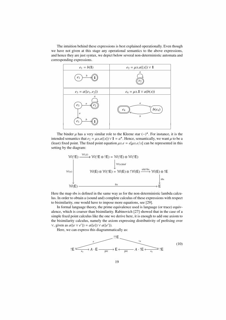
The intuition behind these expressions is best explained operationally. Even thoughwe have not given at this stage any operational semantics to the above expressions,and hence they are just syntax, we depict below several non-deterministic automata andcorresponding expressions.

e1 = b(1) e2 = µx.a({x}) ∨ 1

e1b // 1

e2

a

e3 = a({e1, e2}) e4 = µx.1 ∨ a(b(x))

e3a //

a

��

e2

a

e1b // 1

e4

a))

b(e4)

b

ii

The binder µ has a very similar role to the Kleene star (−)?. For instance, it is theintended semantics that e2 = µx.a({x})∨1 = a?. Hence, semantically, we want µ to be a(least) fixed point. The fixed point equation µx.e = e[µx.e/x] can be represented in thissetting by the diagram:

W(!E) //

W(ε)

��

W(∆)// W(!E ⊗ !E) =W(!E) ⊗W(!E)

W(ε)⊗id��

W(E) ⊗W(!E) =W(E) ⊗ !W(E)id⊗!fix

// W(E) ⊗ !E

sbs��

W(E) fix // E

Here the map sbs is defined in the same way as for the non-deterministic lambda calcu-lus. In order to obtain a (sound and) complete calculus of these expressions with respectto bisimilarity, one would have to impose more equations, see [29].

In formal language theory, the prime equivalence used is language (or trace) equiv-alence, which is coarser than bisimilarity. Rabinovich [27] showed that in the case of asimple fixed point calculus like the one we derive here, it is enough to add one axiom tothe bisimilarity calculus, namely the axiom expressing distributivity of prefixing over∨, given as a({e ∨ e′}) = a({e}) ∨ a({e′}).

Here, we can express this diagrammatically as:

!!Eε

ss

!ε

++!Eκa

// A · E pre// E A · !Epreoo !E

κaoo

(10)

19

This diagram is actually a more general formulation of the Rabinovich distributivityrule, since the starting point !!E = P2

fin(E) at the top involves sets of sets of expressions.To recover the binary version above one should start from {{e1, e2}} ∈ !!E. The commu-tativity of the above diagram says that a({e1∨e2}) = a({e1, e2}), and the right side of thisequation rewrites to a({e1, e2}) = a({e1})∨a({e2}), since pre is a JSL map. The relevanceof capturing this law diagrammatically is that it provides a guideline to which law givestrace semantics in other settings. For instance, we show in the next subsection that forweighted automata, the same diagram can be used to axiomatise trace semantics.

5.4 Weighted automata

We can obtain a syntax for weighted automata in a similar way by switching to themultiset monad M, for a semiring S , and considering the initial algebra E of the functoron SModN:

P 7−→ F +W(P) + S + A · !P,

where S denotes the constant presheaf ∆(S ), and F(n) = M({v1, . . . , vn}), and !P =M(P).

Again, coalgebraically, weighted automata are modelled using the functor F(X) =S ×M(X)A (in Sets). We can describe the above initial algebra as the following isomor-phism.

F +W(E) + S + A · !E[var,fix,val,pre]

�// E

Elements of the set of expressions E(n) ∈ SMod with variables from {v1, . . . , vn} areinductively given by:

– varn(V) where V ⊆ {v1, . . . , vn};– fixn(e) = µvn+1.e, where e ∈ E(n + 1);– s = val(s), for any s ∈ S ;– a(

∑i siei) = pre(κa(

∑i siei));

– 0, s • e, and e + e′ for any e, e′ ∈ E(n) and s ∈ S .

Intuitively, the expression s denotes that the output of a state is s and a(∑

k≤m skek) de-notes a state with m transitions labelled by a, sk to the states denoted by the expressionse1, . . . , em. We depict below two examples of expressions (over the semiring of integers)and the respective (intended) weighted automata they represent.

e1 = b(2 • 1) e2 = µx.a(3x + 2e1) + 1

e1

��

b,2// 1

��0 1

e2

a,3

a,2//

��

e1

��

b,2// 1

��1 0 1

Note that e1 above has output 0 because the expression only specifies the b transitionand no concrete output. Intuitively, the expression e1 specifies a state which has a b

20

transition with weight 2 to a state specified by the expression 1. The latter specifies astate with no transitions and with output 1. The use of + in e2 allows the combinedspecification of transitions and outputs and hence e2 has output 1.

Examples of equations one might want to impose in this calculus include a(r0) = 0,which can be expressed using the diagram:

I = !1 = S 0

(((−)•η(0)

��

!Eκa

// A·!E pre// E

Recent papers [3,7] on generalising the work of Rabinovich, have proposed, in a ratherad hoc fashion, axiomatisations of trace semantics for weighted automata. The verysame diagram (10) capturing Rabinovich’s axiom for non-deterministic automata cannow be interpreted in this weighted setting and it will result in the following axiom —which we present immediately a binary version, for readability.

a(s(e1 + e2)) = a(se1) + a(se2).

(We write se for the singleton multiset s • 1e.)

Final remarks

We have exploited initiality in categories of algebra-valued presheaves EM(T )N, for amonad T on Sets, to modularly obtain a syntactic calculus of expressions as initial alge-bra of a given functor. The theory involved provides a systematic description of severalnon-trivial examples: non-deterministic and weighted lambda calculus and expressionsfor (weighted) automata.

The use of presheaves to describe calculi with binding operators has first been stud-ied by Fiore, Plotkin and Turi. They used set-valued presheaves and did not explore theformalisation of relevant equations for concrete calculi. They have also not exploredtheir theory to derive fixed point calculi. Non-deterministic versions of the lambda cal-culus have appeared in, for instance, [6,26]. The version we derive in this paper ishowever slightly different because we have linearity also in the second argument ofapplication.

As future work, we wish to explore the formalisation of equations that we presentedfor the concrete examples. This opens the door to developing a systematic accountof sound and complete axiomatisations for different equivalences (bisimilarity, trace,failure, etc.). Preliminary work for (generalised) regular expressions and bisimilarityhas appeared in [15,31,30] and for trace semantics in [3].

Acknowledgments

Thanks to Sam Staton for suggesting several improvements.

21

References

1. R. Atkey, P. Johann, and N. Ghani. When is a type refinement an inductive type? In M. Hof-mann, editor, Foundations of Software Science and Computation Structures, number 6604 inLect. Notes Comp. Sci., pages 72–87. Springer, Berlin, 2011.

2. M. Barr and Ch. Wells. Toposes, Triples and Theories. Springer, Berlin, 1985. Revized andcorrected version available from URL: www.cwru.edu/artsci/math/wells/pub/ttt.html.

3. M. Bonsangue, S. Milius, and A. Silva. Sound and complete axiomatizations of coalgebraiclanguage equivalence. ACM Trans. on Computational Logic, 14(1), 2013.

4. F. Borceux. Handbook of Categorical Algebra, volume 50, 51 and 52 of Encyclopedia ofMathematics. Cambridge Univ. Press, 1994.

5. B. Coecke, D. Pavlovic, and J. Vicary. A new description of orthogonal bases. Math. Struct.in Comp. Sci., pages 1–13, 2012.

6. U. de’Liguoro and A. Piperno. Non-deterministic extensions of untyped λ-calculus. Inf. &Comp., 122:149–177, 1995.

7. Z. Esik and W. Kuich. Free iterative and iteration k-semialgebras. CoRR, abs/1008.1507,2010.

8. M. Fiore, G. Plotkin, and D. Turi. Abstract syntax and variable binding. In LICS, pages193–202. IEEE Computer Society, 1999.

9. M. Fiore and S. Staton. Comparing operational models of name-passing process calculi. Inf.& Comp., 2004(4):524–560, 2006.

10. M. Fiore and D. Turi. Semantics of name and value passing. In Logic in Computer Science,pages 93–104. IEEE, Computer Science Press, 2001.

11. J. Goguen, J. Thatcher, E. Wagner, and J. Wright. Initial algebra semantics and continuousalgebras. Journ. ACM, 24(1):68–95, 1977.

12. I. Hasuo, B. Jacobs, and A. Sokolova. Generic trace theory via coinduction. Logical Methodsin Computer Science, 3(4:11), 2007.

13. B. Jacobs. Semantics of weakening and contraction. Ann. Pure & Appl. Logic, 69(1):73–106,1994.

14. B. Jacobs. Categorical Logic and Type Theory. North Holland, Amsterdam, 1999.15. B. Jacobs. A bialgebraic review of deterministic automata, regular expressions and lan-

guages. In K. Futatsugi, J.-P. Jouannaud, and J. Meseguer, editors, Essays Dedicated toJoseph A. Goguen, volume 4060 of Lecture Notes in Computer Science, pages 375–404.Springer, 2006.

16. B. Jacobs. Bases as coalgebras. In A. Corradini, B. Klin, and C. Cırstea, editors, Conferenceon Algebra and Coalgebra in Computer Science (CALCO 2011), number 6859 in Lect. NotesComp. Sci., pages 237–252. Springer, Berlin, 2011. Extended version appears in LogicalMethods in Computer Science.

17. B. Jacobs. Introduction to Coalgebra. Towards Mathematics of States and Observations.2012. Book, in preparation; version 2 available from www.cs.ru.nl/B.Jacobs/CLG/JacobsCoalgebraIntro.pdf.

18. A. Joyal and I. Moerdijk. Algebraic Set Theory. Number 220 in LMS. Cambridge Univ.Press, 1995.

19. B. Klin. Bialgebras for structural operational semantics: An introduction. Theor. Comp. Sci.,412(38):5043–5069, 2011.

20. A. Kock. Bilinearity and cartesian closed monads. Math. Scand., 29:161–174, 1971.21. A. Kock. Closed categories generated by commutative monads. Journ. Austr. Math. Soc.,

XII:405–424, 1971.

22

22. J. Lambek. A fixed point theorem for complete categories. Math. Zeitschr., 103:151–161,1968.

23. E.G. Manes. Algebraic Theories. Springer, Berlin, 1974.24. S. Mac Lane. Categories for the Working Mathematician. Springer, Berlin, 1971.25. R. Møgelberg and S. Staton. Linearly-used state in models of call-by-value. In A. Corradini,

B. Klin, and C. Cırstea, editors, Conference on Algebra and Coalgebra in Computer Science(CALCO 2011), number 6859 in Lect. Notes Comp. Sci., pages 293–313. Springer, Berlin,2011.

26. M. Pagani and S. Ronchi della Rocca. Solvability in resource lambda-calculus. In Proceed-ings of the 13th international conference on Foundations of Software Science and Computa-tional Structures, FOSSACS’10, pages 358–373, Berlin, Heidelberg, 2010. Springer-Verlag.

27. Alexander Moshe Rabinovich. A complete axiomatisation for trace congruence of finite statebehaviors. In Stephen D. Brookes, Michael G. Main, Austin Melton, Michael W. Mislove,and David A. Schmidt, editors, MFPS, volume 802 of Lecture Notes in Computer Science,pages 530–543. Springer, 1993.

28. J. Rutten. Universal coalgebra: a theory of systems. Theor. Comput. Sci., 249(1):3–80, 2000.29. A. Silva. Kleene coalgebra. PhD thesis, Radboud University Nijmegen, 2010.30. A. Silva, F. Bonchi, M. Bonsangue, and J. Rutten. Generalizing the powerset construction,

coalgebraically. In Proc. FSTTCS 2010, volume 8 of LIPIcs, pages 272–283, 2010.31. A. Silva, M. Bonsangue, and J. Rutten. Non-deterministic kleene coalgebras. Logical Meth-

ods in Computer Science, 6(3), 2010.32. T. Uustalu, V. Vene, and A. Pardo. Recursion schemes from comonads. Nordic Journ.

Comput., 8(3):366–390, 2001.

23