Page 1
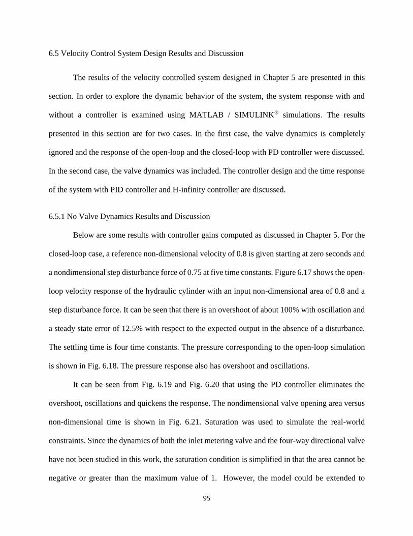
INLET METERING PUMP ANALYSIS AND EXPERIMENTAL EVALUATION
WITH APPLICATION FOR FLOW CONTROL
_______________________________________
A Dissertation
presented to
the Faculty of the Graduate School
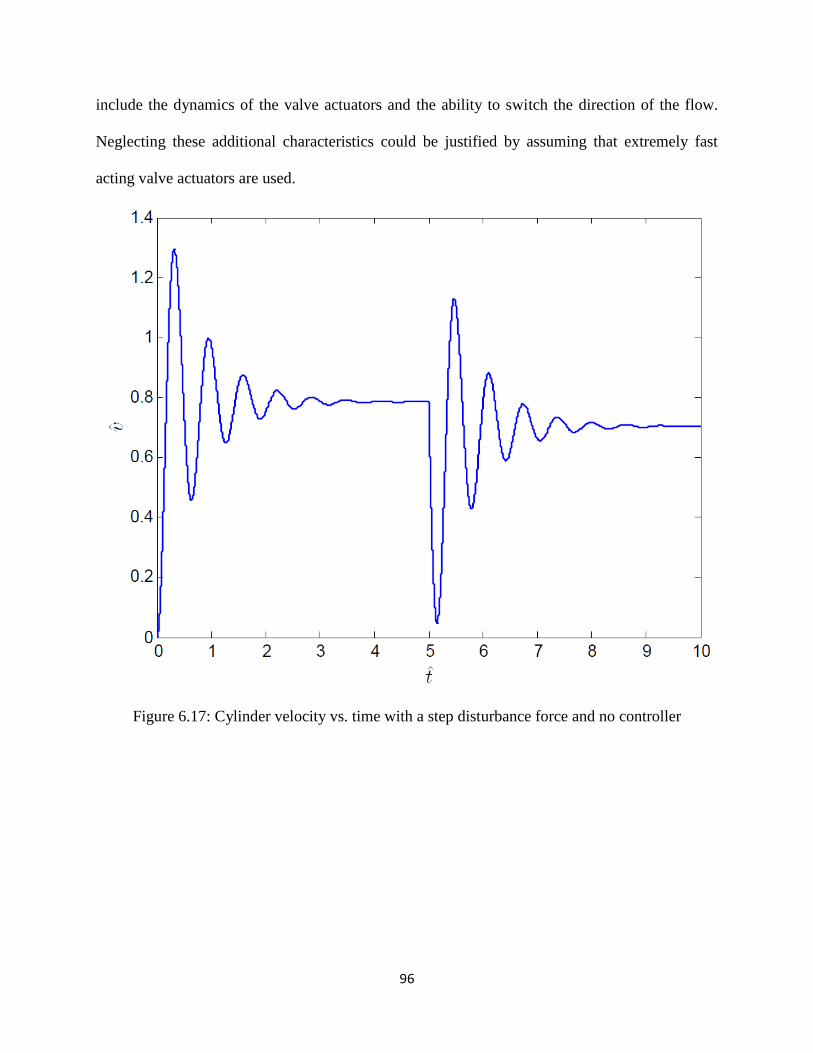
at the University of Missouri-Columbia
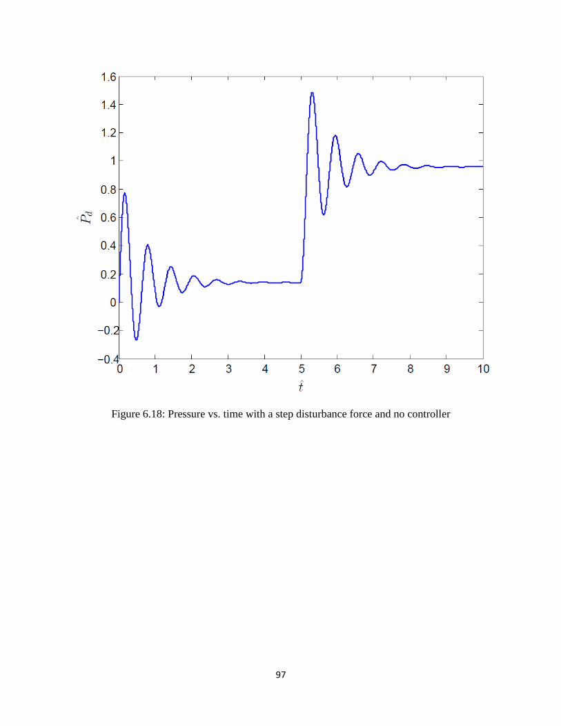
_______________________________________________________
In Partial Fulfillment
of the Requirements for the Degree
Doctor of Philosophy
_____________________________________________________
by
HASAN H. ALI
Dr. Roger Fales, Dissertation Supervisor
December 2017
Page 2
The undersigned, appointed by the dean of the Graduate School, have examined the
dissertation entitled
INLET METERING PUMP ANALYSIS AND EXPERIMENTAL EVALUATION
WITH APPLICATION FOR FLOW CONTROL
presented by Hasan Hamad Ali, a candidate for the degree of doctor of philosophy, and
hereby certify that, in their opinion, it is worthy of acceptance.
Professor Roger Fales
Professor Noah Manring
Professor Craig Kluever
Professor Steven Borgelt
Professor Stephen Montgomery-Smith
Page 3
ii
ACKNOWLEDGEMENTS
I would like to express my sincere gratitude to Dr. Roger Fales for his effort and
contribution to my research. The completion of my Ph.D. degree would not have been
possible without his guidance and assistance.
I would also like to thank Dr. Noah Manring, Dr. Craig Kluever, Dr. Steven
Borgelt, and Dr. Stephen Montgomery-Smith for taking the time to serve on my
dissertation committee. I am appreciative of their ongoing support throughout this work.
I would also like to take the opportunity to thank our partners at Caterpillar: Jeff
Kuehn, Jeremy Peterson, Viral Mehta, Hongliu Du, and Randy Harlow for both the
financial support and collective engineering experience that they contributed to this
project. I am honored to have collaborated with this team of engineers. I am also grateful
for the prototype they were able to provide.
I would like to thank the faculty of the Mechanical and Aerospace department at
MU for helping me to excel in my field of interest.
Finally, I take this opportunity to express the profound gratitude to my family for
their love and continuous support.
Page 4
iii
TABLES OF CONTENTS
ACKNOWLEDGEMENTS ................................................................................................ ii
LIST OF FIGURES .......................................................................................................... vii
LIST OF TABLES ............................................................................................................. xi
LIST OF SYMBOLS ........................................................................................................ xii
ABSTRACT ..................................................................................................................... xvi
1 INTRODUCTION ....................................................................................................... 1
1.1 Background ............................................................................................................. 1
1.2 System Description ................................................................................................. 3
1.3 Velocity Control System ......................................................................................... 4
1.4 Contribution of the Present Work ........................................................................... 7
1.5 Dissertation Outline ................................................................................................ 7
2 LITERATURE REVIEW ............................................................................................ 9
2.1 Introduction ............................................................................................................. 9
2.2 Variable Displacement Pump ................................................................................. 9
2.3 Fixed Displacement Pump .................................................................................... 15
2.4 Switched Systems ................................................................................................. 17
2.5 Fuel Injection Systems .......................................................................................... 19
2.6 Cavitation .............................................................................................................. 22
Page 5
iv
2.7 Literature Review Summary ................................................................................. 23
3 INLET-METERED PUMP EFFICIENCY ................................................................ 25
3.1 Introduction ........................................................................................................... 25
3.2 Modelling and Analysis ........................................................................................ 26
3.2.1 Flow Model ........................................................................................................ 26
3.2.2 Torque Model..................................................................................................... 29
3.3 Model Nondimensionalization .............................................................................. 35
4 EXPERIMENTAL SETUP ........................................................................................ 38
4.1 Introduction ........................................................................................................... 38
4.2 Test Setup.............................................................................................................. 38
4.3 Steady State Testing .............................................................................................. 43
4.4 Transient Testing .................................................................................................. 44
4.5 Inlet-Metering Valve and Pump Components ...................................................... 44
5 Velocity Control System Design ............................................................................... 53
5.1 Introduction ........................................................................................................... 53
5.2 System Modelling ................................................................................................. 54
5.3 Stability Analysis .................................................................................................. 57
5.4 Performance Analysis ........................................................................................... 58
5.4.1 No Valve Dynamics ........................................................................................... 59
Page 6
v
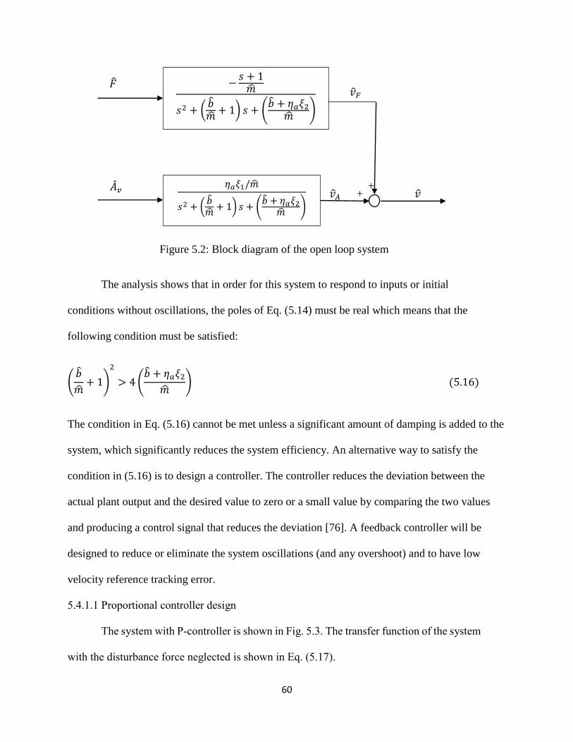
5.4.1.1 Proportional controller design ......................................................................... 60
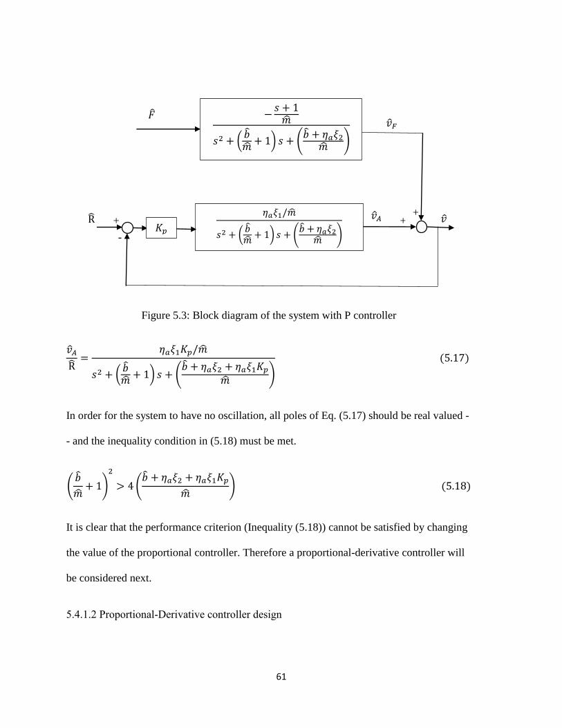
5.4.1.2 Proportional-Derivative controller design ...................................................... 61
5.4.2 Including the Valve Dynamics........................................................................... 64
5.4.2.1 Limitation Imposed by the Time Delay .......................................................... 66
5.4.2.2 PID-Controller Design .................................................................................... 67
5.4.2.3 H∞-Controller Design ..................................................................................... 67
5.4.2.4 Two Degree of Freedom Controller Design ................................................... 67
6 RESULTS AND DISCUSSION ................................................................................ 76
6.1 Introduction ........................................................................................................... 76
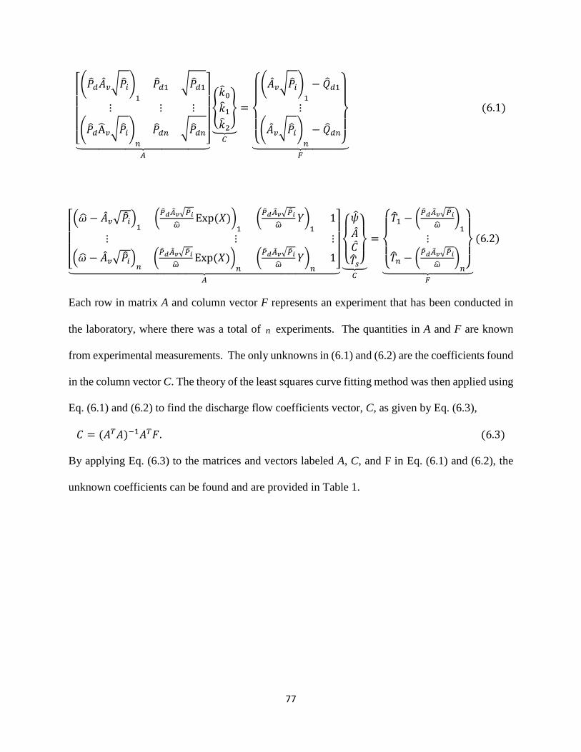
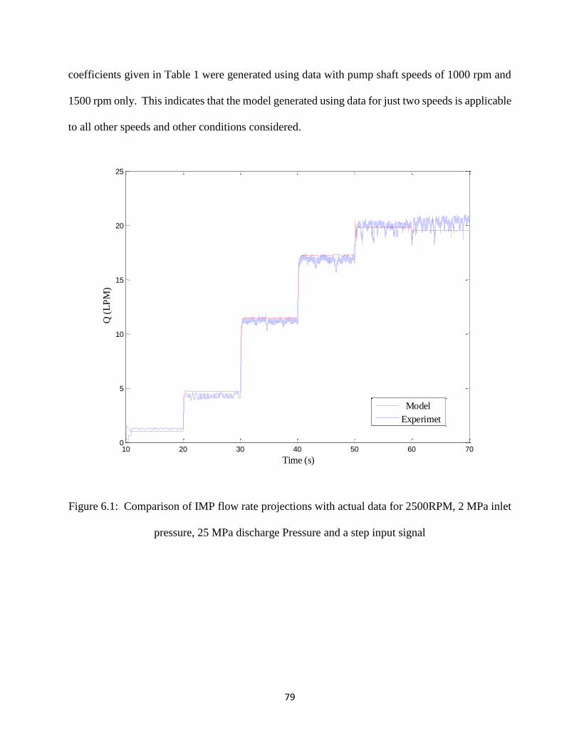
6.2 Determination of the Coefficients in Eqs. (3.29) and (3.31) ................................ 76
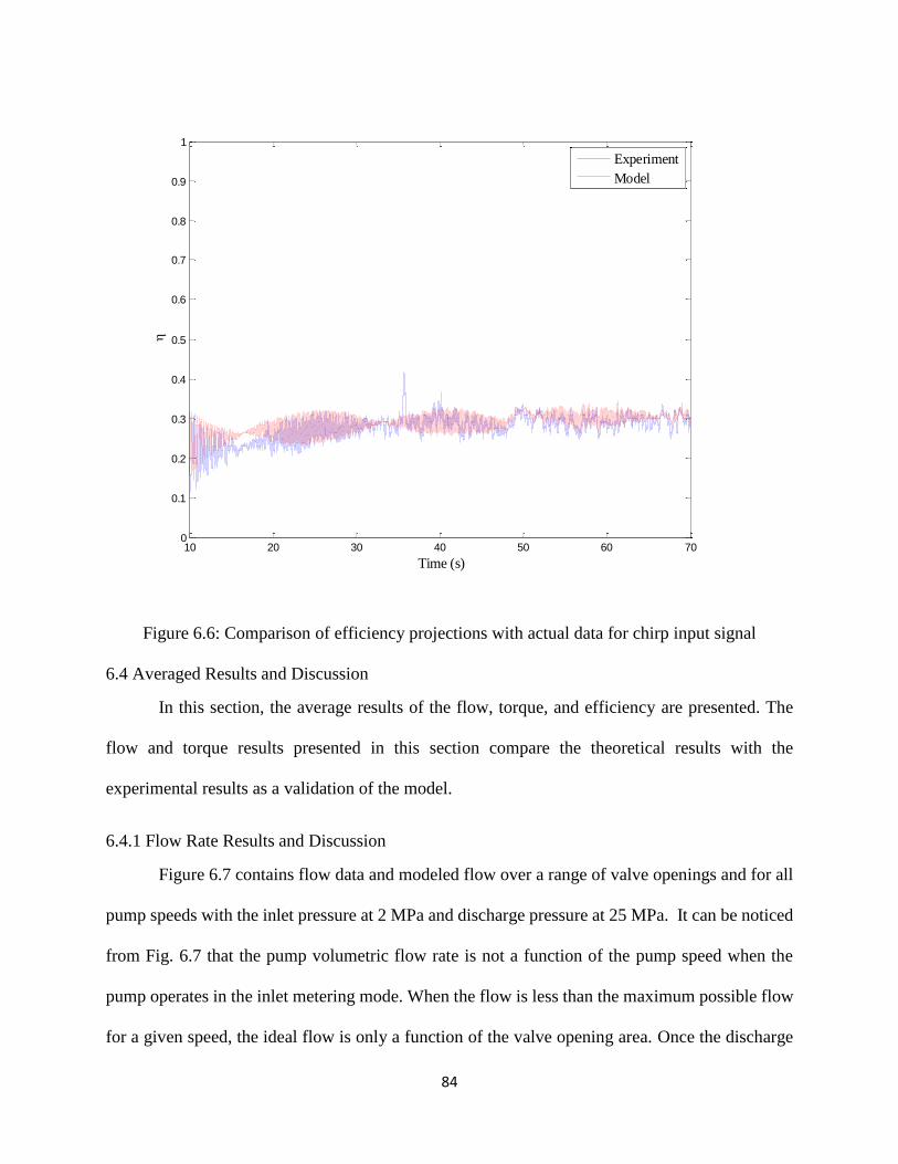
6.3 Instantanous Results and Discussion ................................................................... 78
6.4 Avaraged Results and Discussion ......................................................................... 84
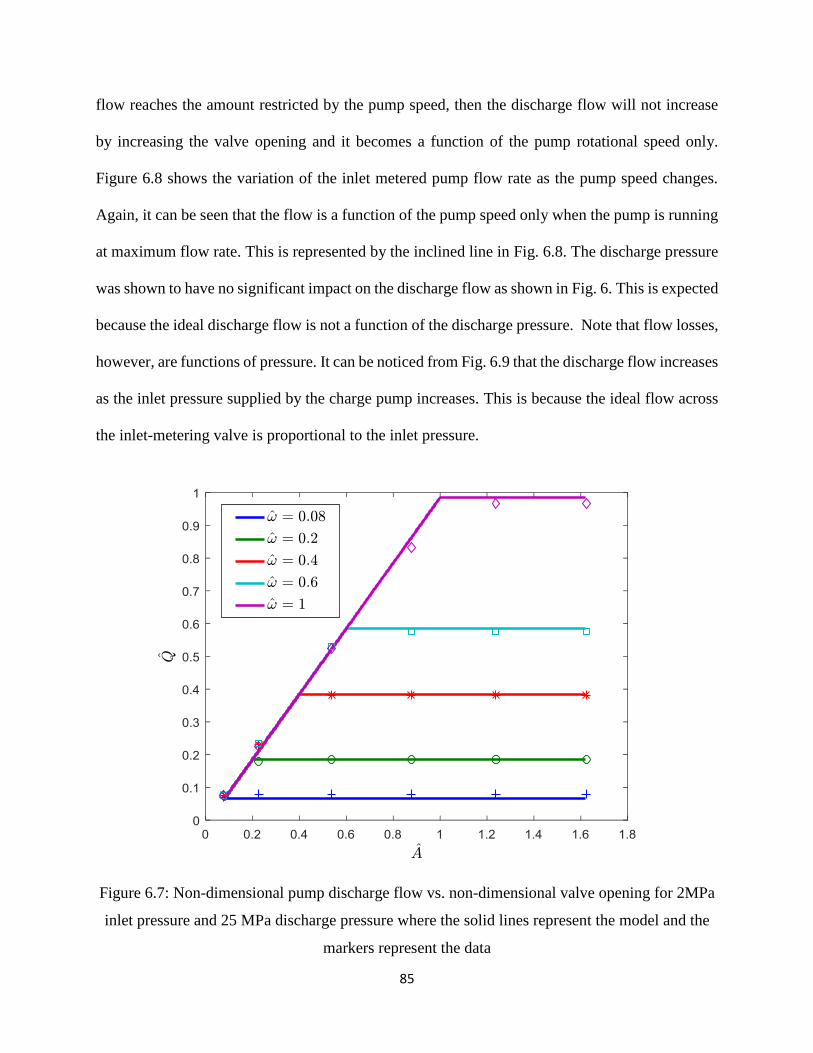
6.4.1 Flow Rate Results and Discussion ..................................................................... 84
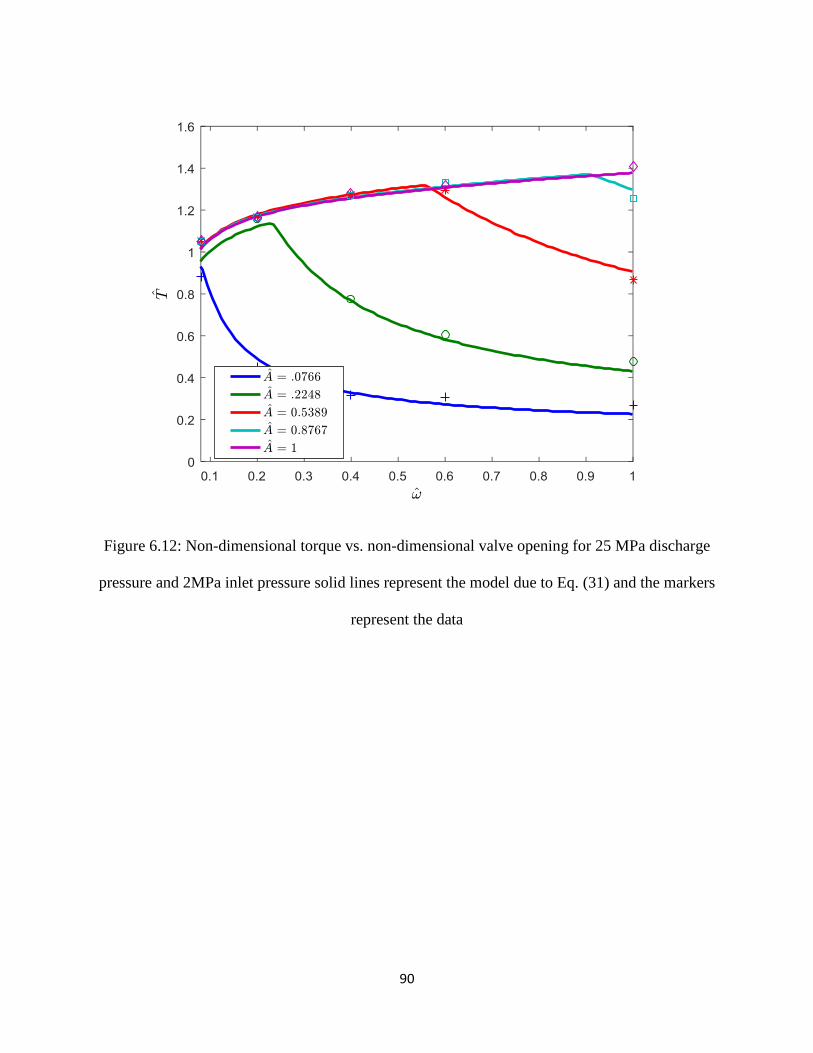
6.4.2 Torque Results and Discussion .......................................................................... 88
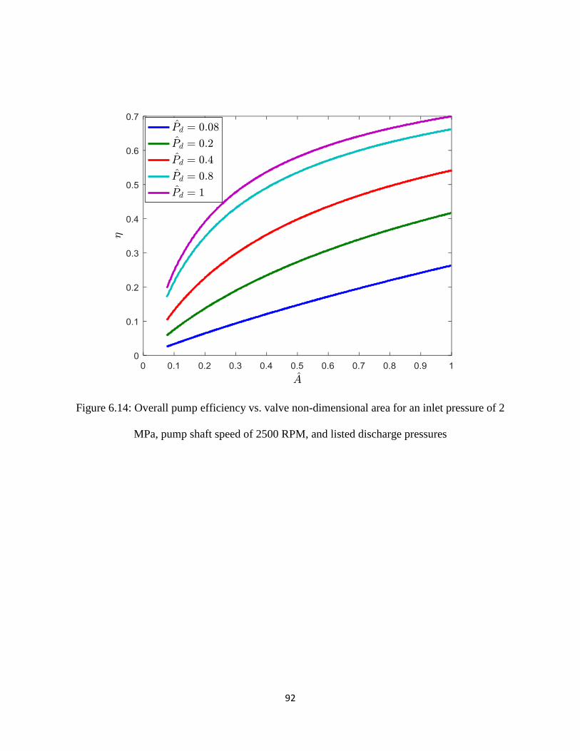
6.4.3 Efficiency Results and Discussion ..................................................................... 91
6.5 Velocity Control System Design Results and Discussion .................................... 95
6.5.1 No Valve Dynamics Results and Discussion ..................................................... 95
5.4.1 Including the Valve Dynamics Results and Discussion .................................. 100
Page 7
vi
7 CONCLUSION AND FUTURE WORK ................................................................ 107
7.1 Introduction ......................................................................................................... 107
7.2 Conclusions ......................................................................................................... 108
7.3 Recommendations for Future Work.................................................................... 110
REFERENCES ............................................................................................................... 112
APPENDICES ................................................................................................................ 123
VITA ............................................................................................................................... 135
Page 8
vii
LIST OF FIGURES
Figure Page
Figure 1.1. A Schematic of Hydrostatic Transmission ...................................................... 2
Figure 1.2. Variable Displacement Pump .......................................................................... 3
Figure 1.3. The Inlet Metering System ................................................................................ 5
Figure 1.4. The Inlet Metering velocity control System .................................................... 6
Figure 3.1. Inlet Metering Valve and Fixed Displacement Single Piston Pump System 25
Figure 3.2. Stribeck curve ................................................................................................ 30
Figure 3.3. Piston Volume and Pressure .......................................................................... 31
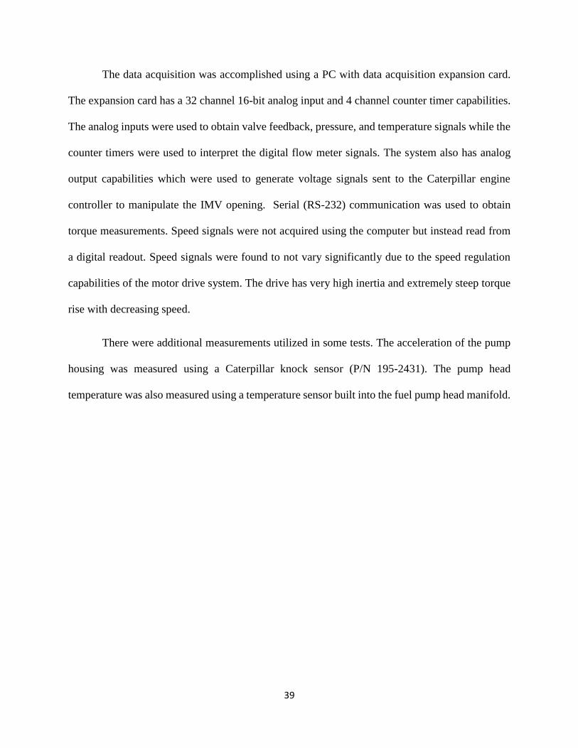
Figure 4.1. Inlet metering pump testing circuit diagram ................................................. 40
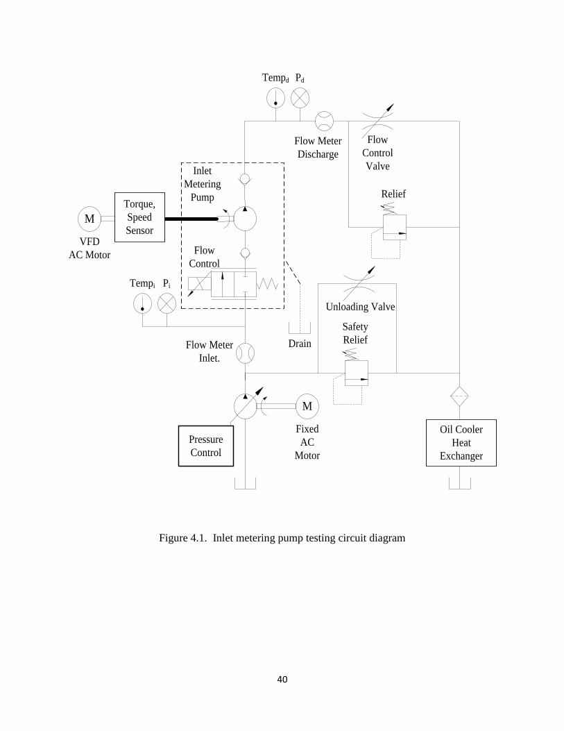
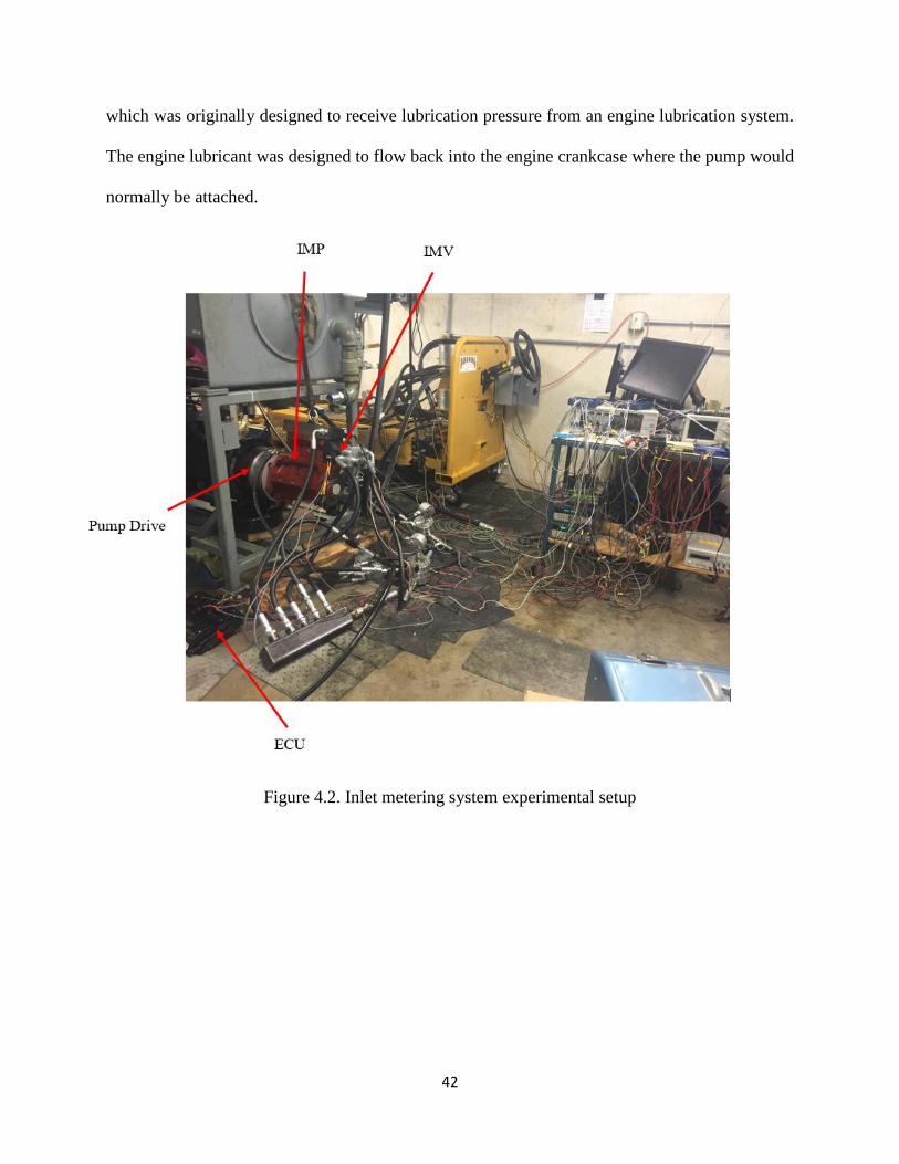
Figure 4.2. Inlet metering system experimental setup ........................................................ 42
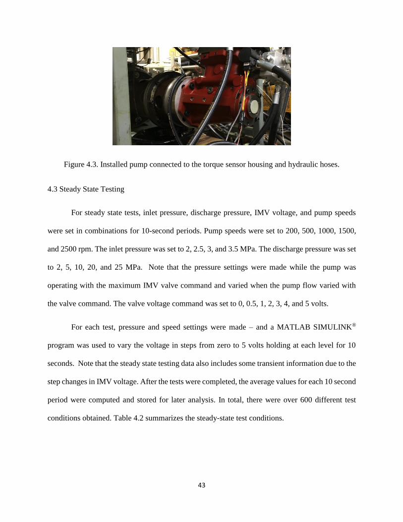
Figure 4.3. Installed Pump Connected to the Torque sensor housing and hoses ............. 43
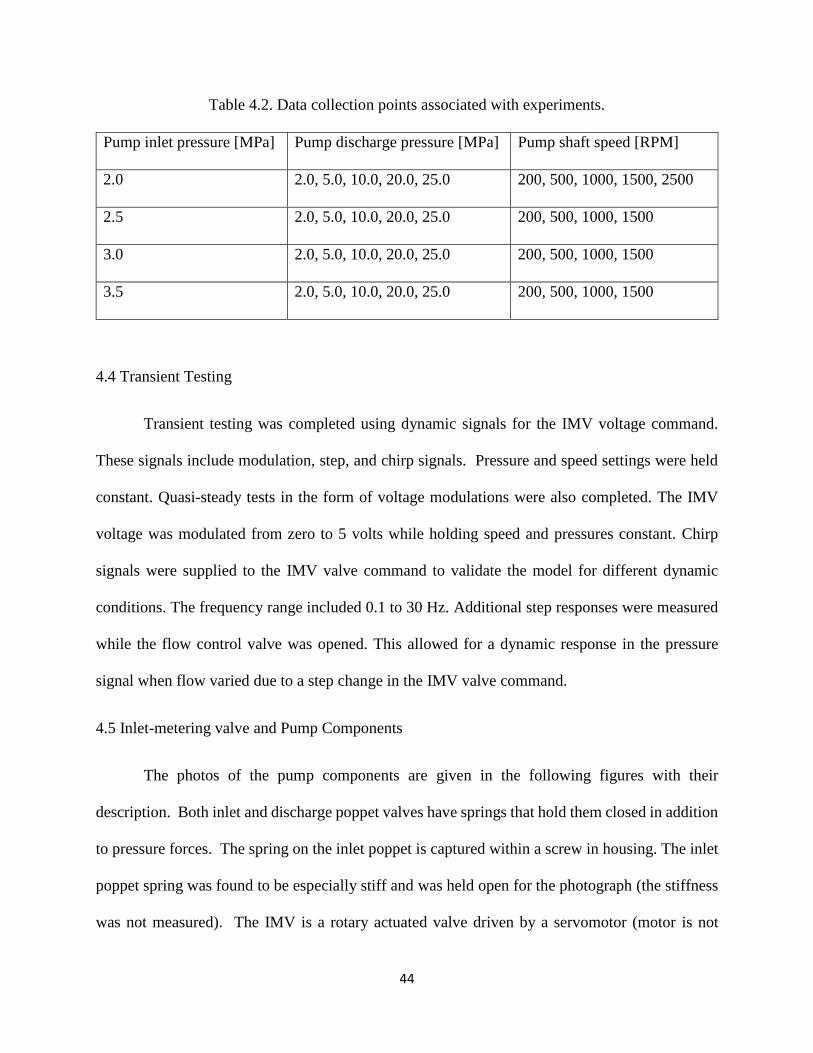
Figure 4.4. Piston Side View ............................................................................................ 45
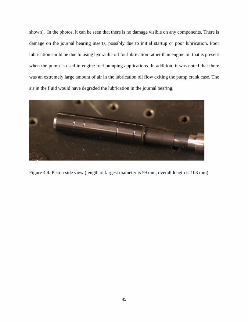
Figure 4.5. Piston Crown ................................................................................................. 46
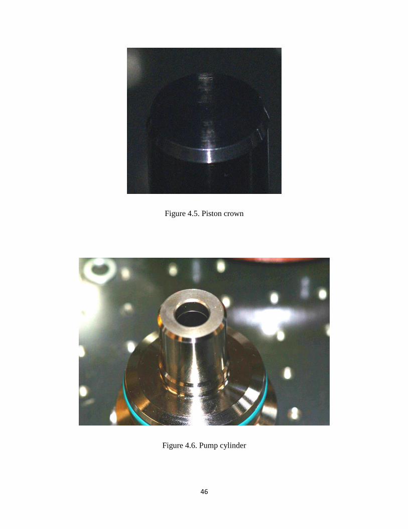
Figure 4.6. Pump Cylinder ............................................................................................... 46
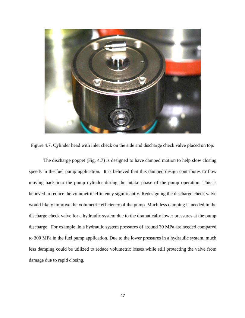
Figure 4.7. Cylinder Head with Inlet Check on the Side and Discharge Check Valve
Placed on Top ................................................................................................................... 47
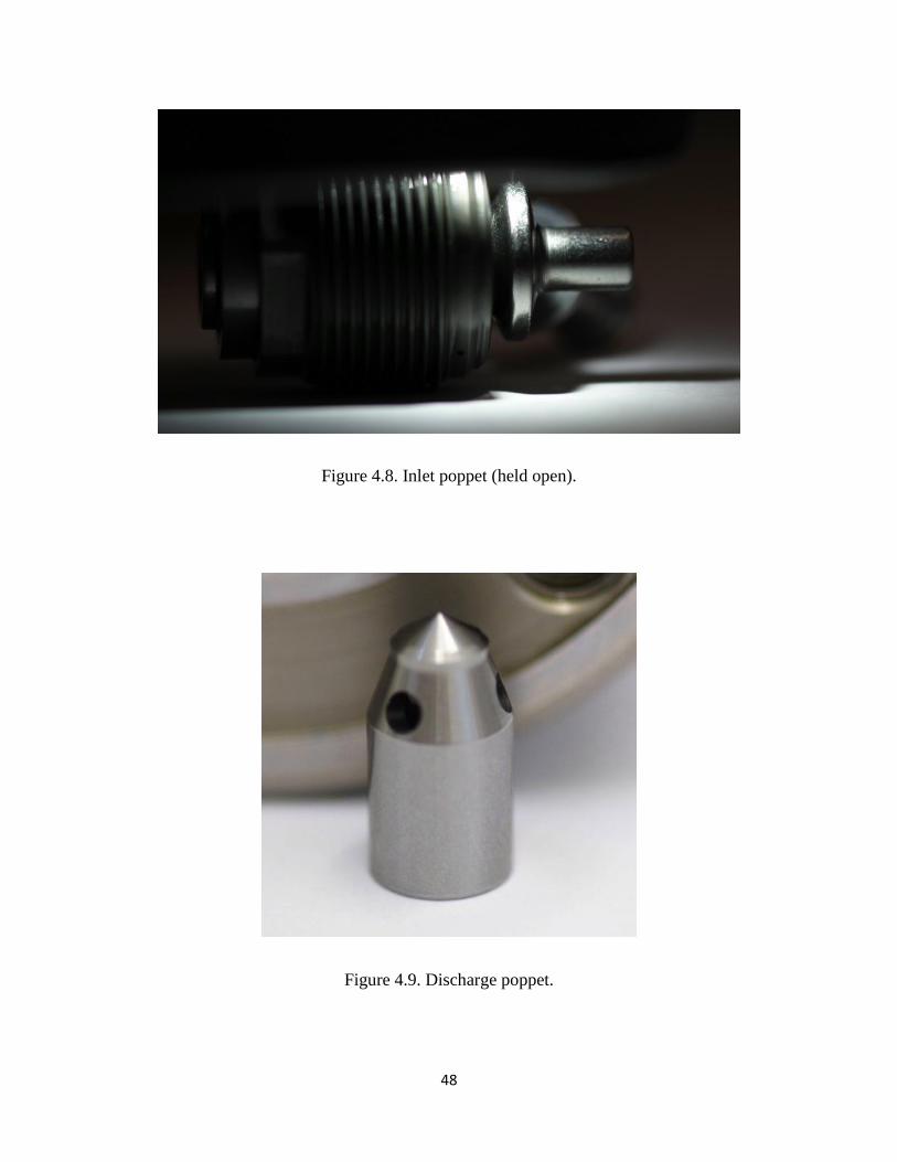
Figure 4.8. Inlet Poppet (held open) ................................................................................ 48
Figure 4.9. Discharge Poppet ........................................................................................... 48
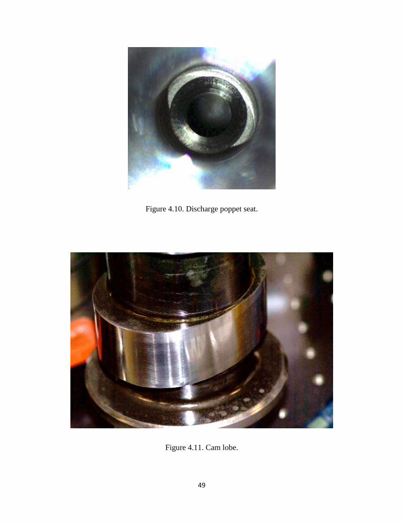
Figure 4.10. Discharge Poppet Seat ................................................................................. 49
Figure 4.11. Cam Lobe .................................................................................................... 49
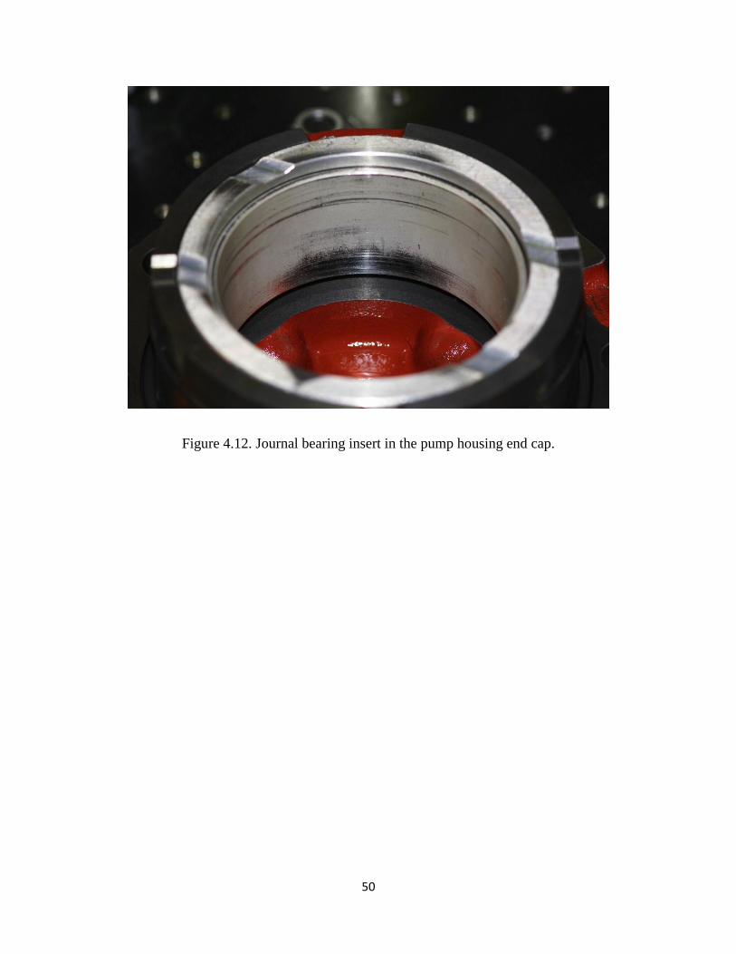
Figure 4.12. Journal Bearing Insert in the Pump Housing End Cap ................................... 50
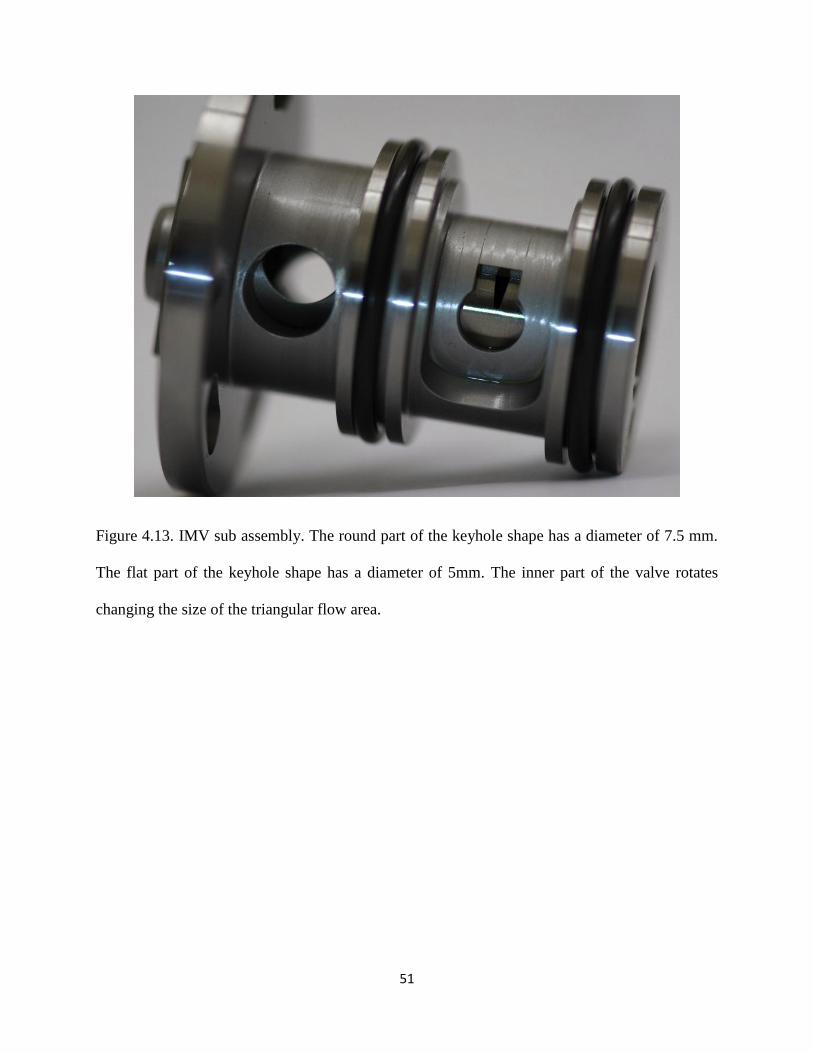
Figure 4.13. Inlet Metering Valve Sub Assembly .............................................................. 51
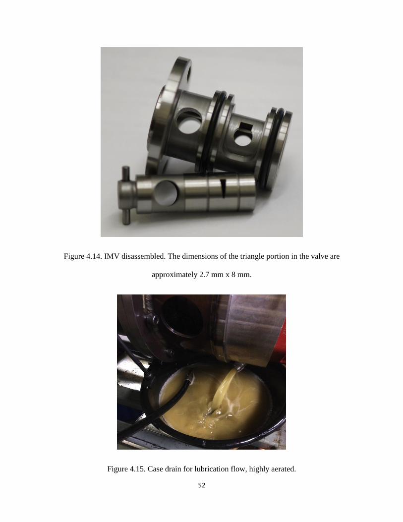
Figure 4.14. Inlet Metering Valve disassembled................................................................. 52
Page 9
viii
Figure 4.15. Case drain for lubrication flow .................................................................... 52
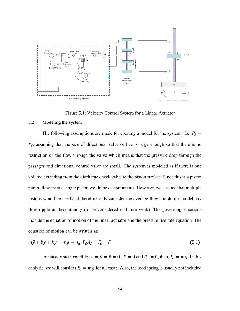
Figure 5.1. Velocity Control System for a Linear Actuator ............................................ 53
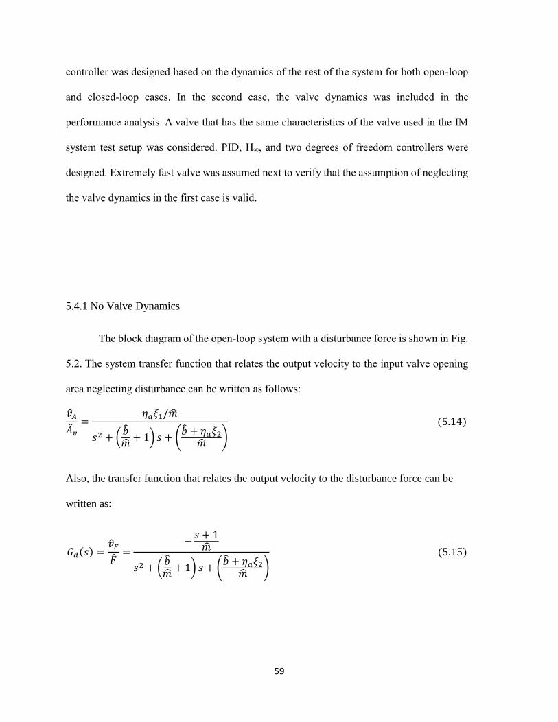
Figure 5.2. Block Diagram of the Open Loop System ....................................................... 59
Figure 5.3. Block Diagram of the System with P Controller .............................................. 60
Figure 5.4. Block diagram of the system with PD controller.............................................. 62
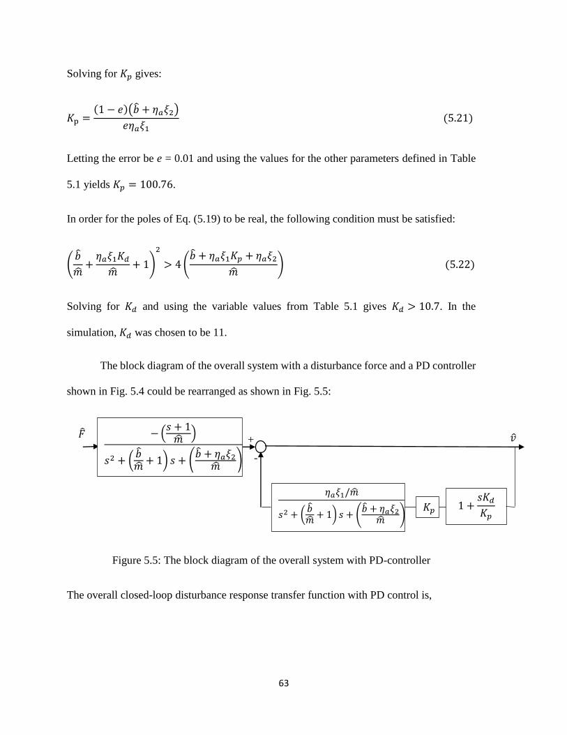
Figure 5.5. The Block Diagram of the overall System with PD-Controller ........................ 63
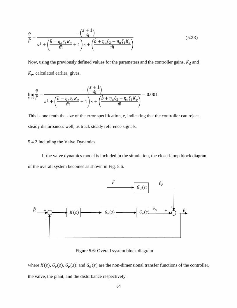
Figure 5.6. Overall System Block Diagram ..................................................................... 64
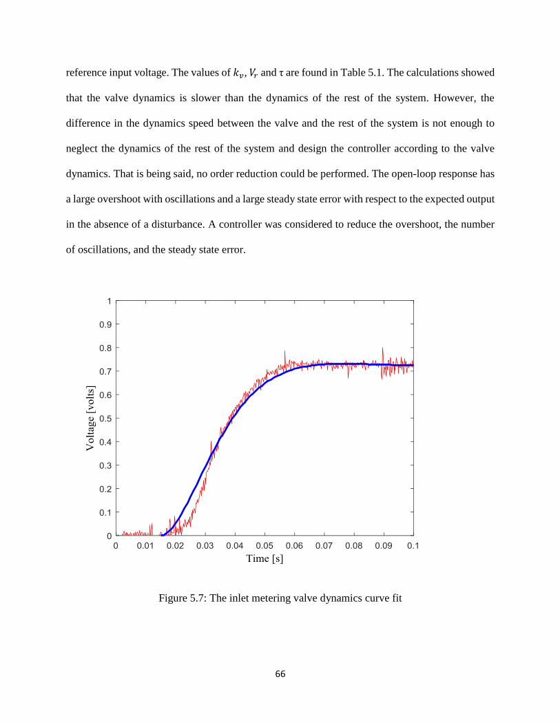
Figure 5.7. The Inlet Metering Valve Dynamics Curve Fit ............................................. 66
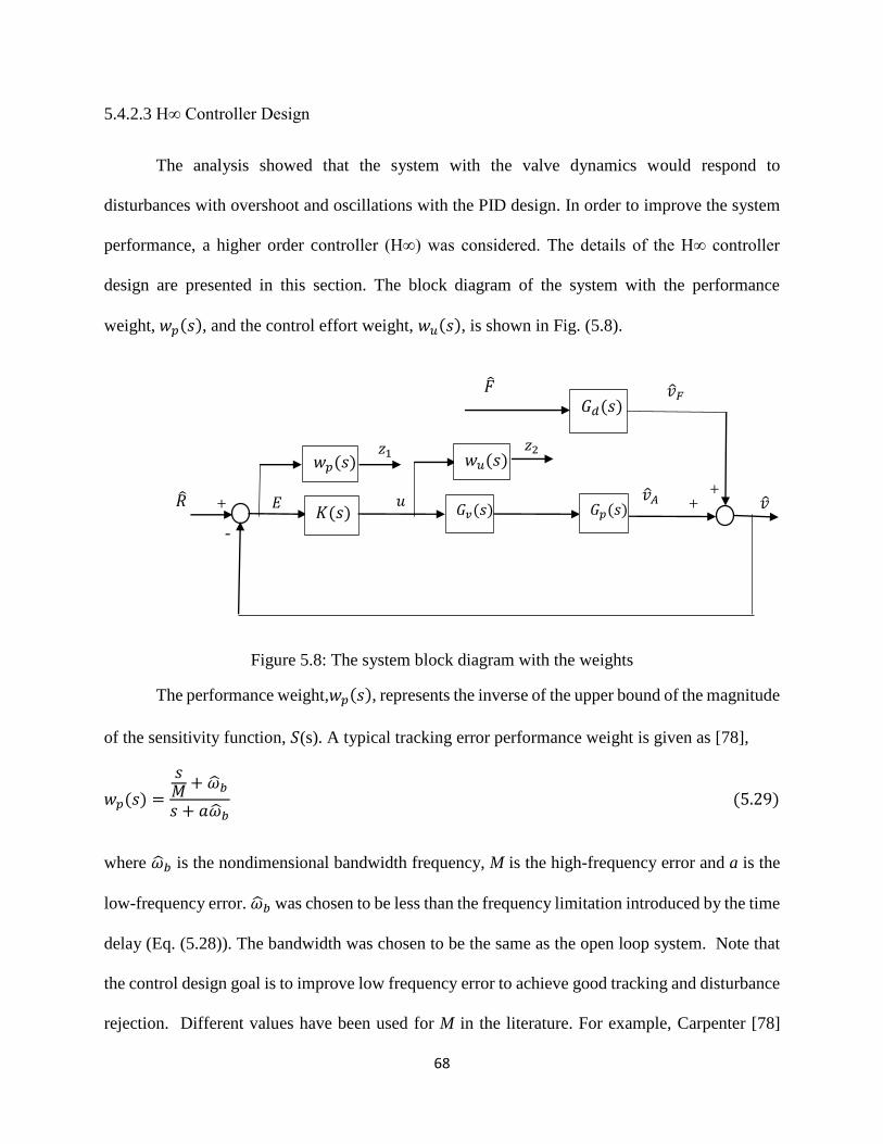
Figure 5.8. The System Block Diagram with the Weights ................................................. 68
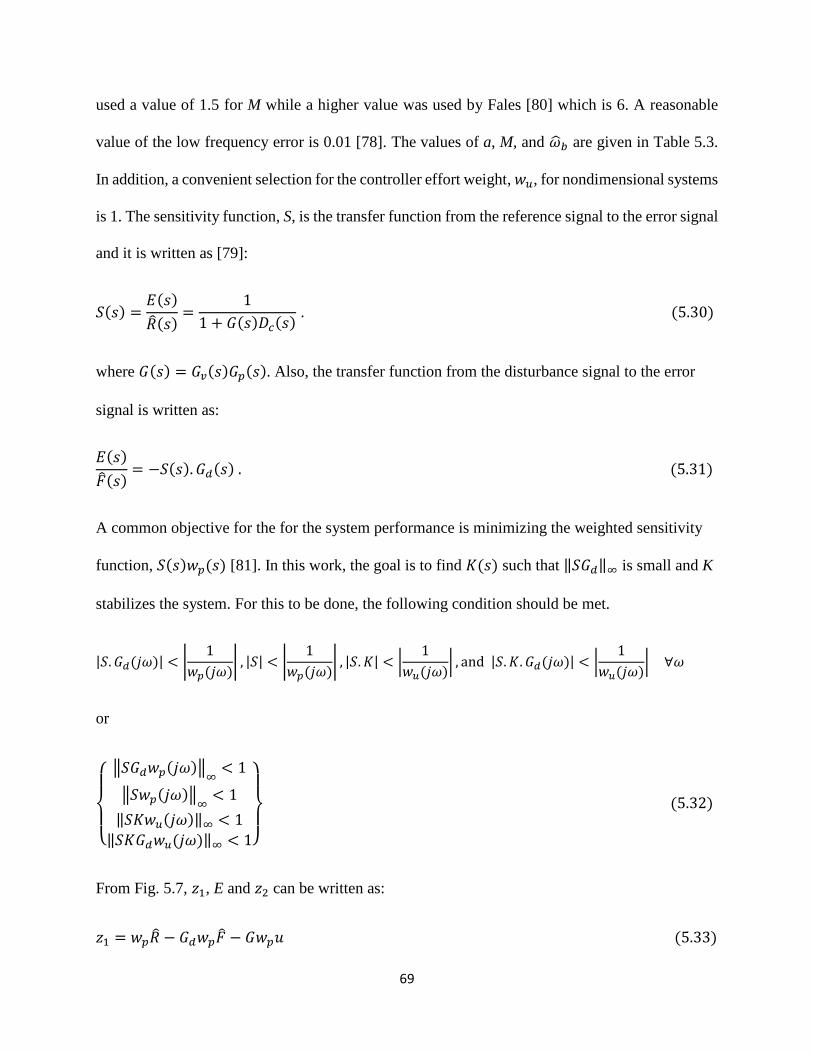
Figure 5.9. The generalized plant ...................................................................................... 70
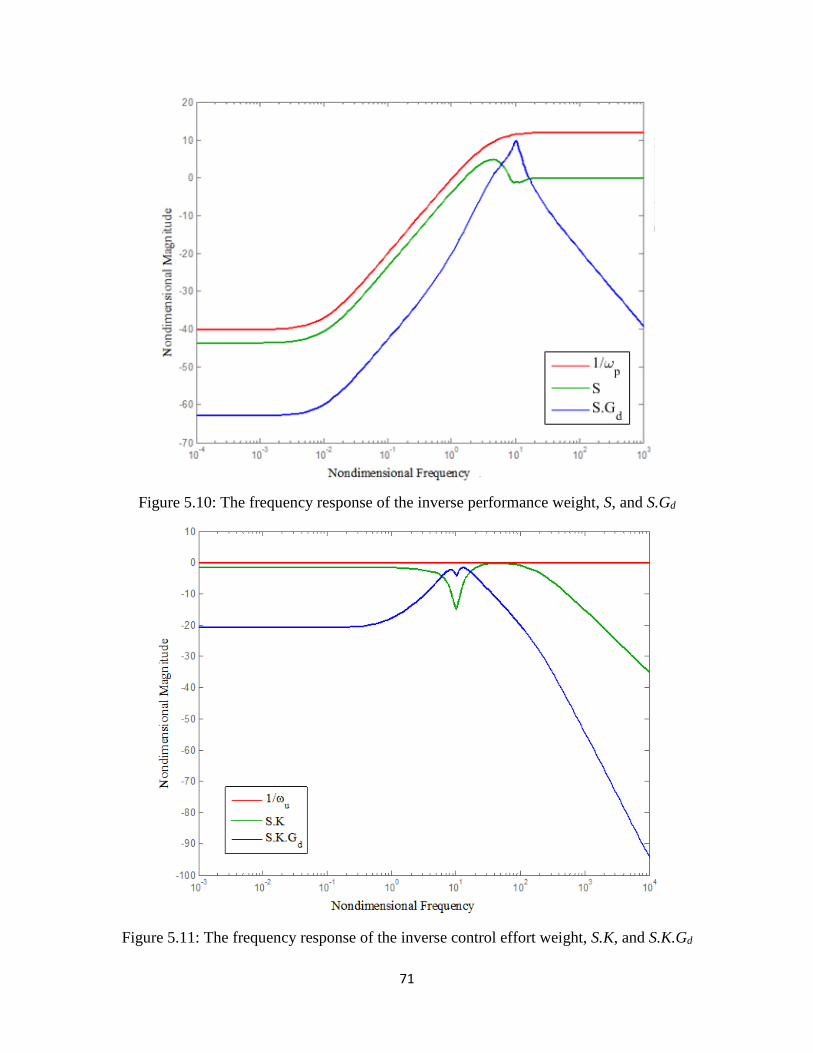
Figure 5.10. The frequency response of the performance weight, S, and S.Gd................. 71
Figure 5.11. The frequency response of the Control Effort weight, S.K, and S.K.Gd ....... 71
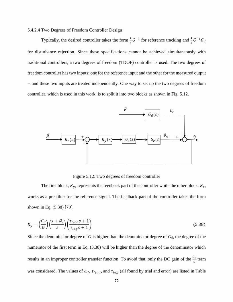
Figure 5.12. Two degrees of freedom controller ............................................................. 72
Figure 6.1. Comparison of IMP flow rate projections with actual data for 2500RPM, 2
MPa inlet pressure, 25 MPa discharge Pressure and a step input signal .......................... 79
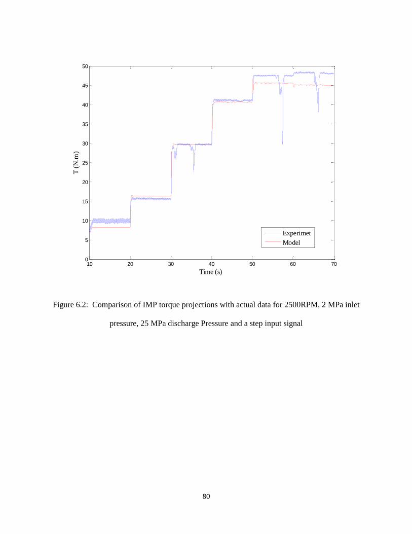
Figure 6.2. Comparison of IMP torque projections with actual data for 2500RPM, 2 MPa
inlet pressure, 25 MPa discharge Pressure and a step input signal ................................... 80
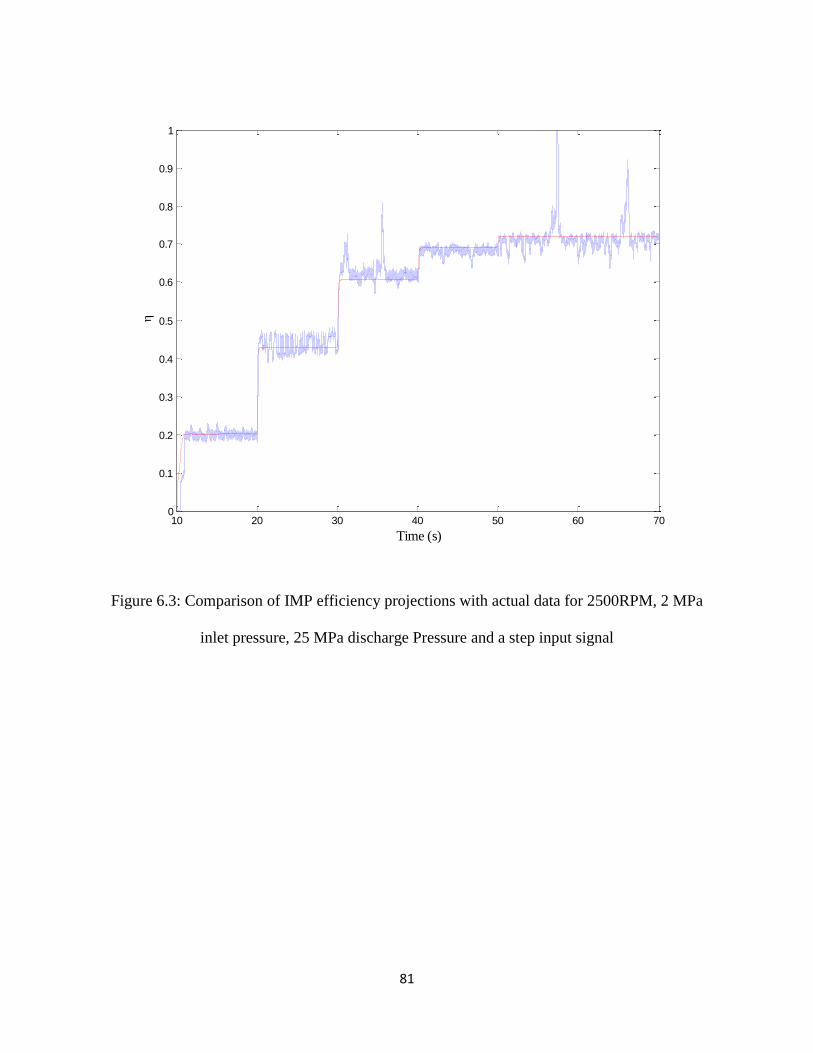
Figure 6.3. Comparison of IMP efficiency projections with actual data for 2500RPM, 2
MPa inlet pressure, 25 MPa discharge Pressure and a step input signal .......................... 81
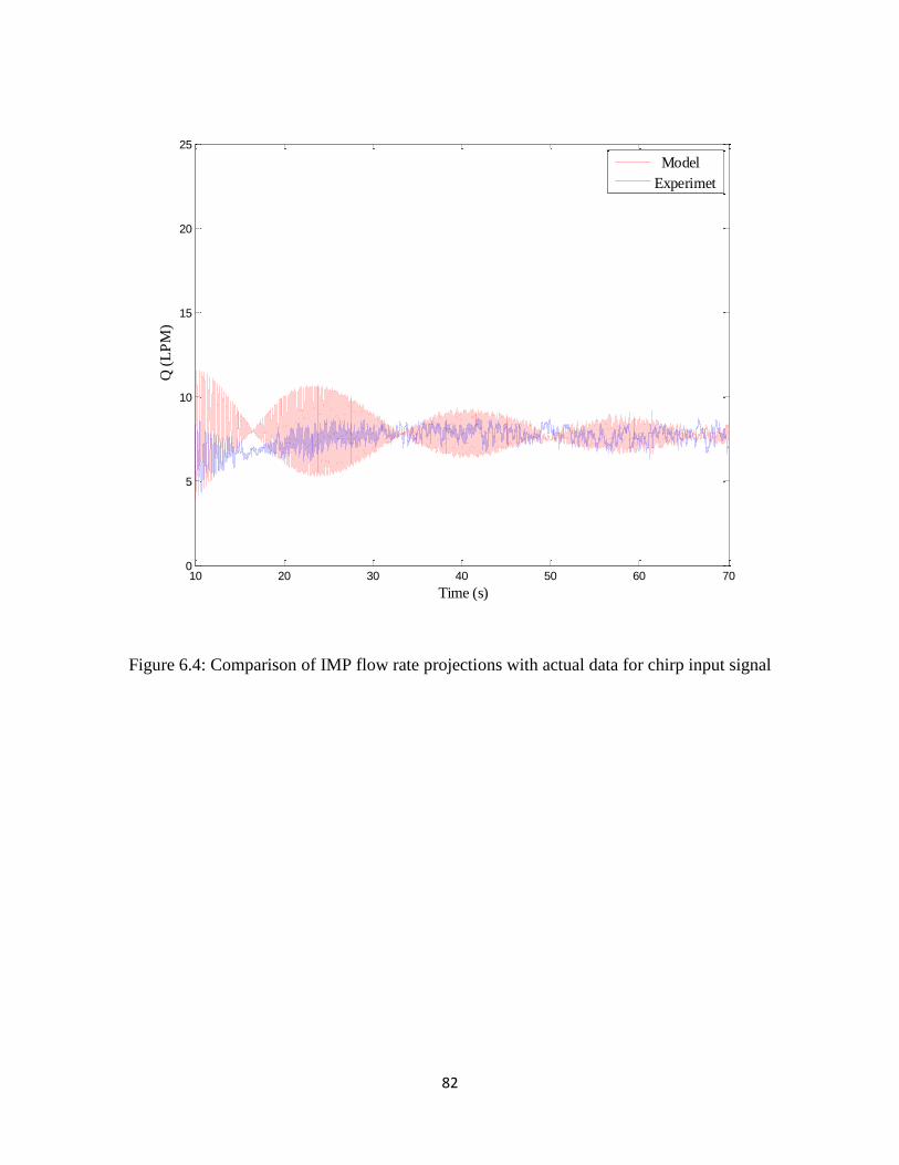
Figure 6.4. Comparison of IMP flow rate projections with actual data for chirp input
signal ................................................................................................................................. 82
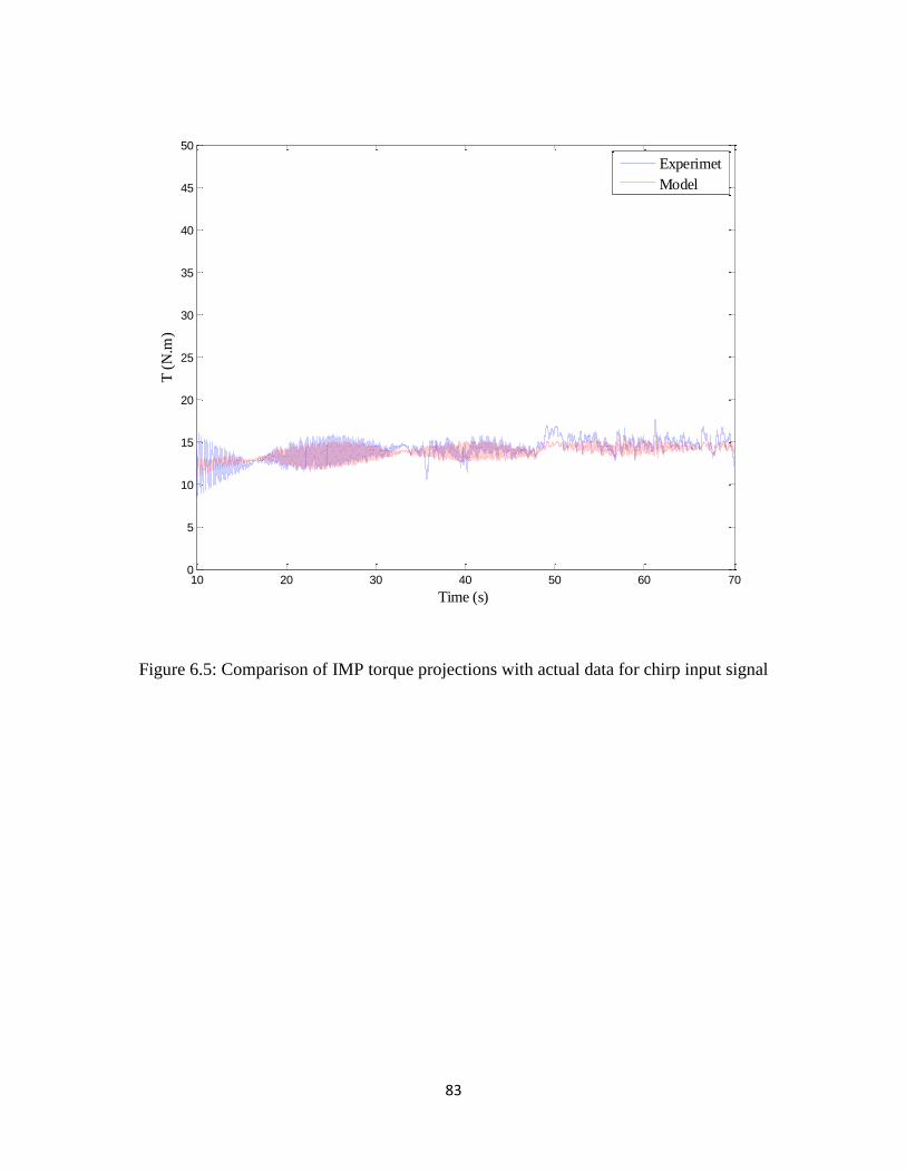
Figure 6.5. Comparison of IMP torque projections with actual data for chirp input signal
........................................................................................................................................... 83
Page 10
ix
Figure 6.6. Comparison of IMP efficiency projections with actual data for chirp input
signal ................................................................................................................................. 84
Figure 6.7. Non-dimensional pump discharge flow vs. non-dimensional valve opening
for 2MPa inlet pressure and 25 MPa discharge pressure where the solid lines represent
the model and the markers represent the data ................................................................... 85
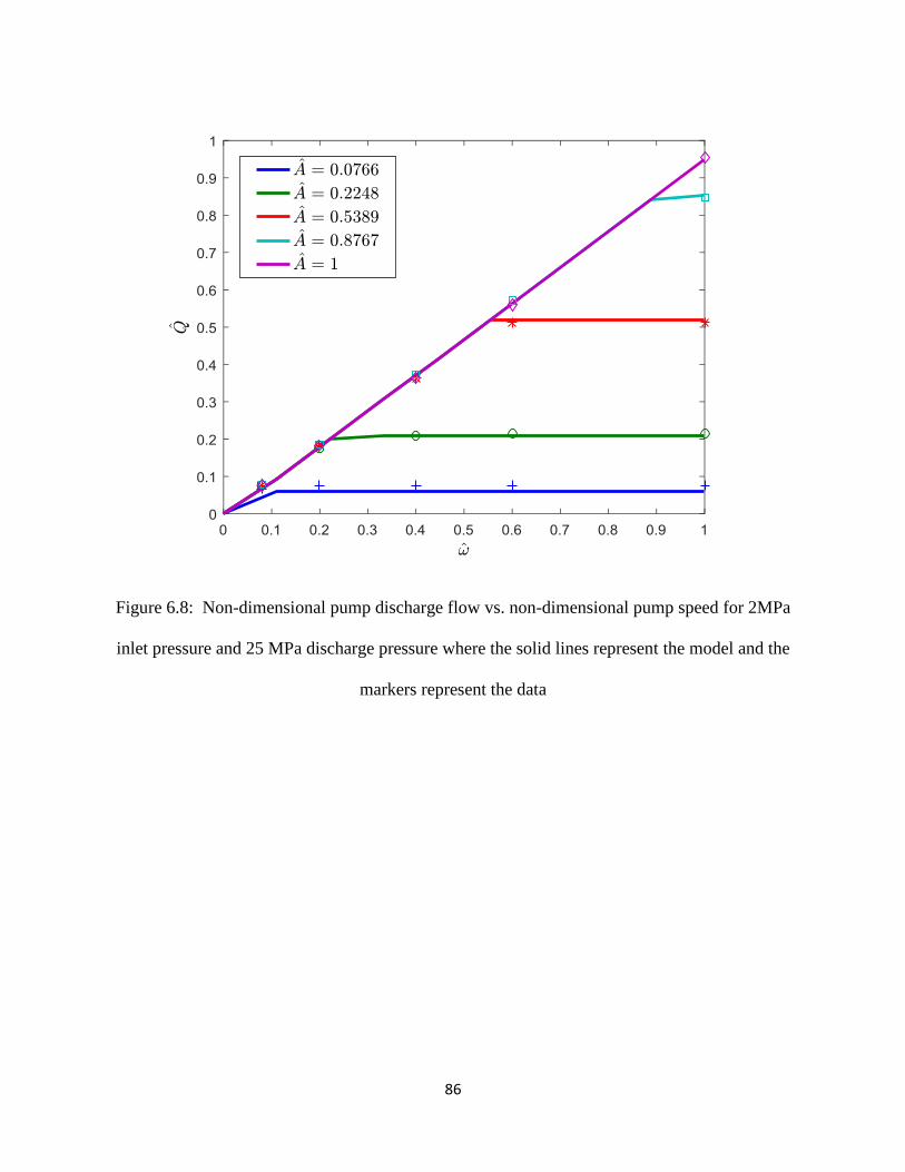
Figure 6.8. Non-dimensional pump discharge flow vs. non-dimensional pump speed for
2MPa inlet pressure and 25 MPa discharge pressure where the solid lines represent the
model and the markers represent the data ......................................................................... 86
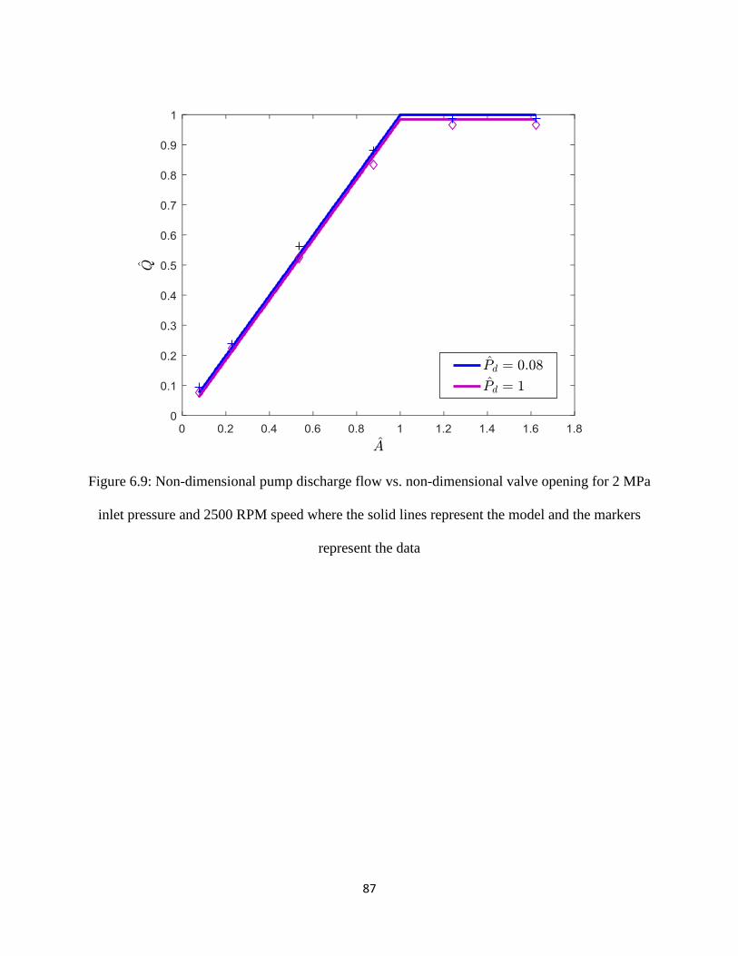
Figure 6.9. Non-dimensional pump discharge flow vs. non-dimensional valve opening for
2 MPa inlet pressure and 2500 RPM speed where the solid lines represent the model and
the markers represent the data........................................................................................... 87
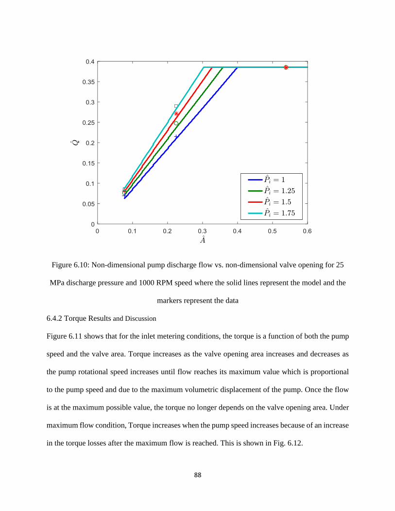
Figure 6.10. Non-dimensional pump discharge flow vs. non-dimensional valve opening
for 25 MPa discharge pressure and 1000 RPM speed where the solid lines represent the
model and the markers represent the data ......................................................................... 88
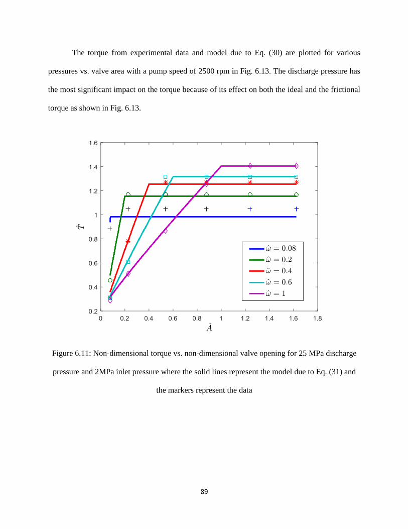
Figure 6.11. Non-dimensional torque vs. non-dimensional valve opening for 25 MPa
discharge pressure and 2MPa inlet pressure where the solid lines represent the model due to
Eq. (31) and the markers represent the data......................................................................... 89
Figure 6.12. Non-dimensional torque vs. non-dimensional valve opening for 25 MPa
discharge pressure and 2MPa inlet pressure solid lines represent the model due to Eq. (31)
and the markers represent the data ...................................................................................... 90
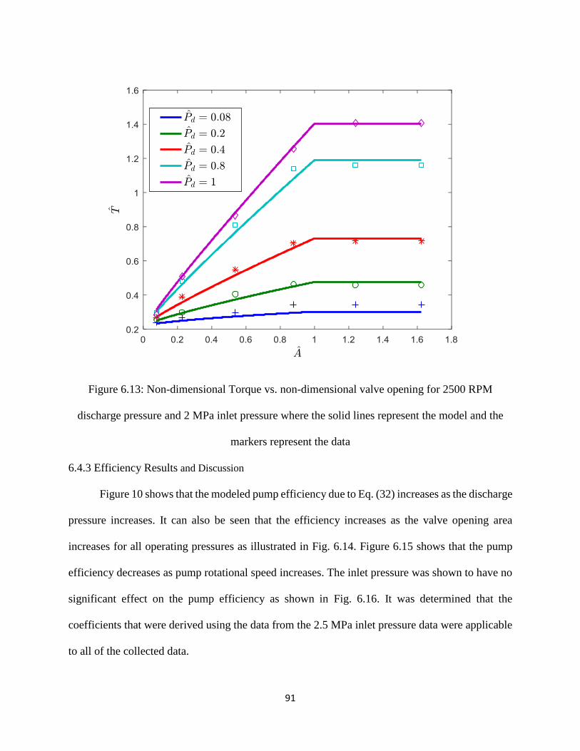
Figure 6.13. Non-dimensional Torque vs. non-dimensional valve opening for 2500 RPM
discharge pressure and 2 MPa inlet pressure where the solid lines represent the model and the
markers represent the data .................................................................................................. 91
Page 11
x
Figure 6.14. Overall pump efficiency vs. valve non-dimensional area for an inlet pressure of
2 MPa, pump shaft speed of 2500 RPM, and listed discharge pressures .............................. 92
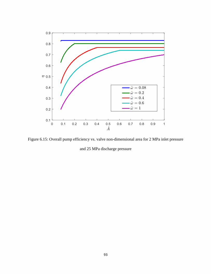
Figure 6.15. Overall pump efficiency vs. valve non-dimensional area for 2 MPa inlet
pressure and 25 MPa discharge pressure ............................................................................. 93
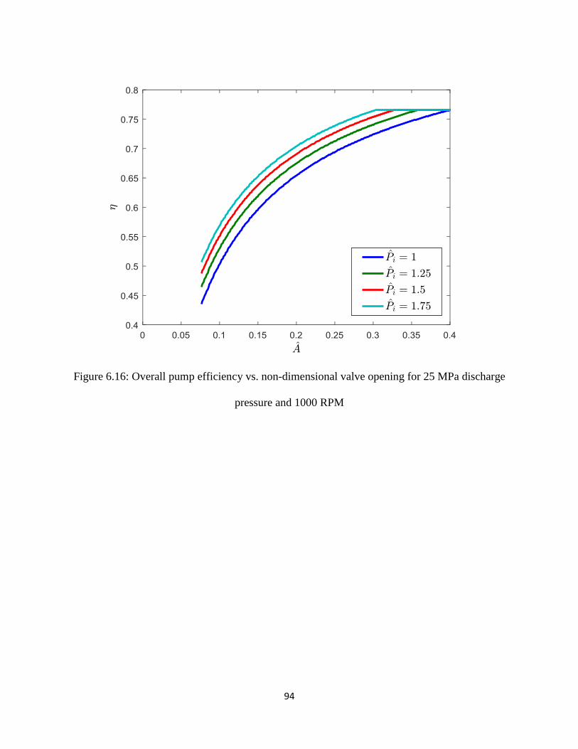
Figure 6.16. Overall pump efficiency vs. non-dimensional valve opening for 25 MPa
discharge pressure and 1000 RPM ...................................................................................... 94
Figure 6.17. Cylinder velocity vs. time with a step disturbance force and no controller 88
Figure 6.18. Pressure vs. time with a step disturbance force and no controller ................... 97
Figure 6.19. Cylinder velocity vs. time with PD controller and a step disturbance force .... 98
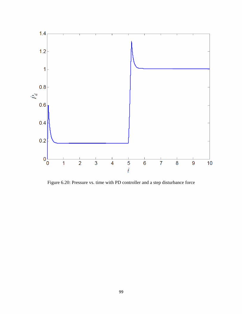
Figure 6.20. Pressure vs. time with PD controller and a step disturbance force .................. 99
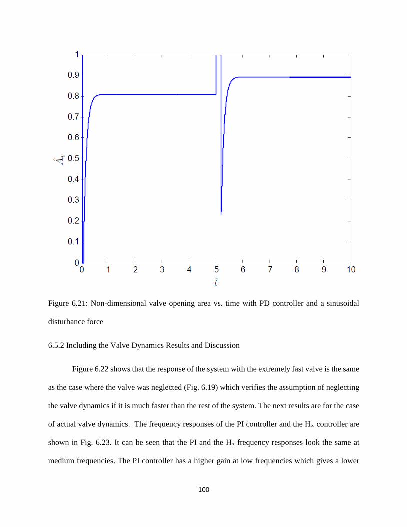
Figure 6.21. Non-dimensional valve opening area vs. time with PD controller and a
sinusoidal disturbance force.............................................................................................. 100
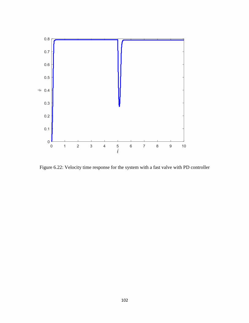
Figure 6.22. Velocity time response for the system with a fast valve with PD controller . 102
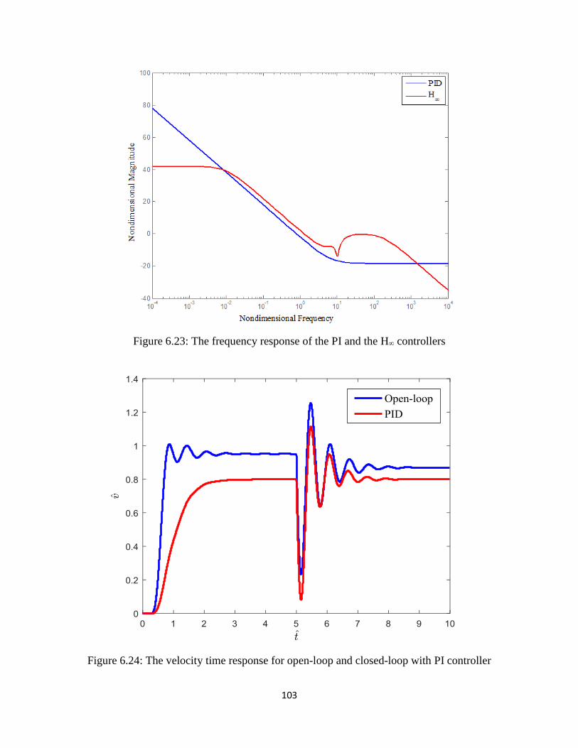
Figure 6.23. The frequency response of the PID and the H∞ controllers ........................... 103
Figure 6.24. The velocity time response for open-loop and closed-loop with PID controller
......................................................................................................................................... 103
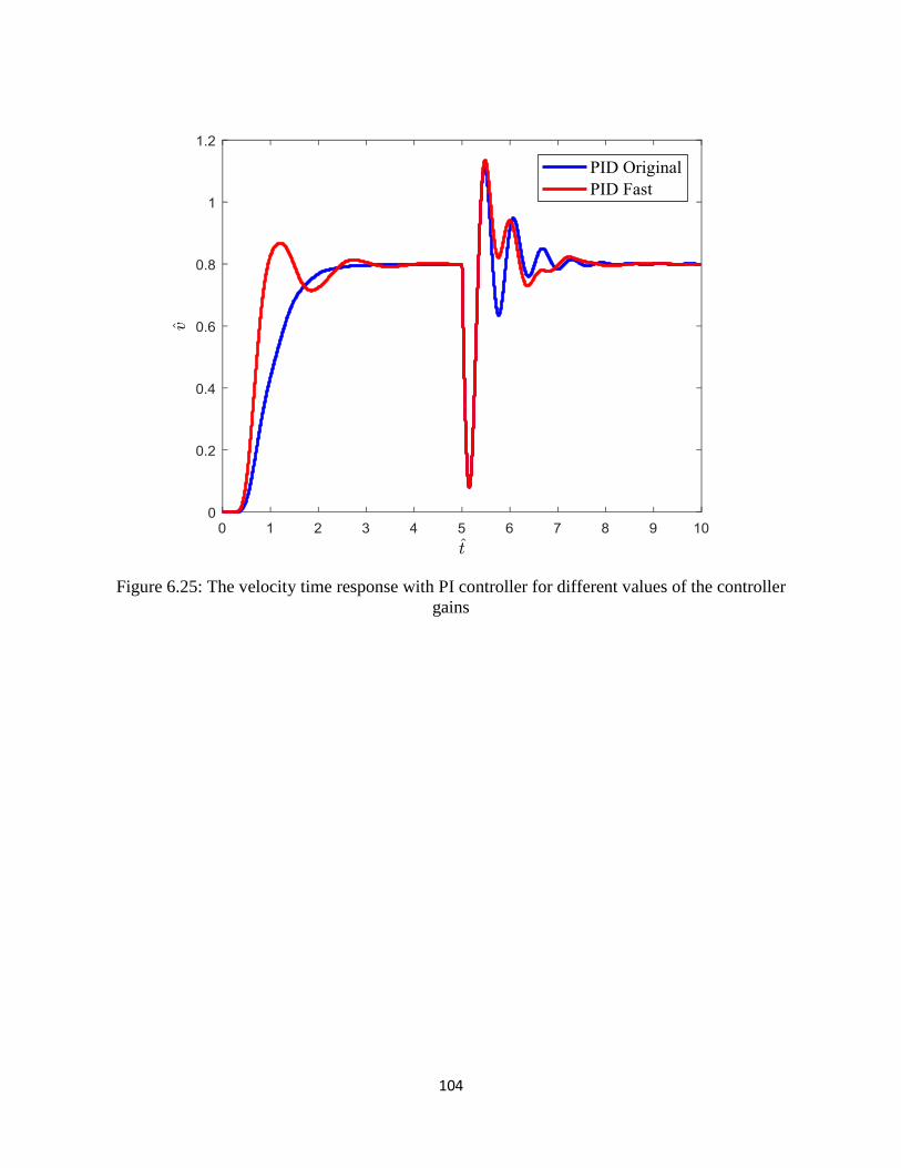
Figure 6.25. The velocity time response with PID controller for different values of the
controller gains ................................................................................................................. 104
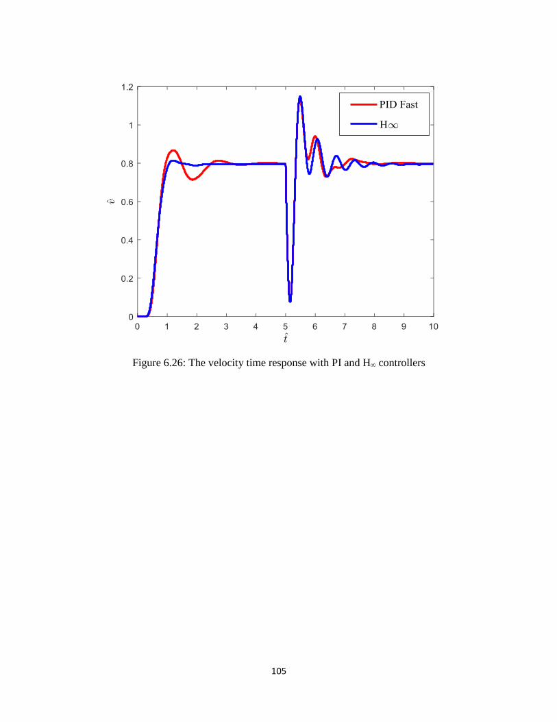
Figure 6.26. The velocity time response with PID and H∞ controllers .......................... 104
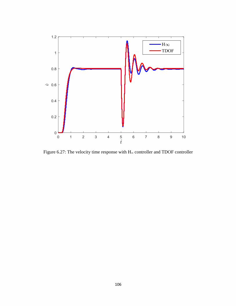
Figure 6.27. The velocity time response with H∞ controller and TDOF controller ........... 105
Page 12
xi
LIST OF TABLES
Table Page
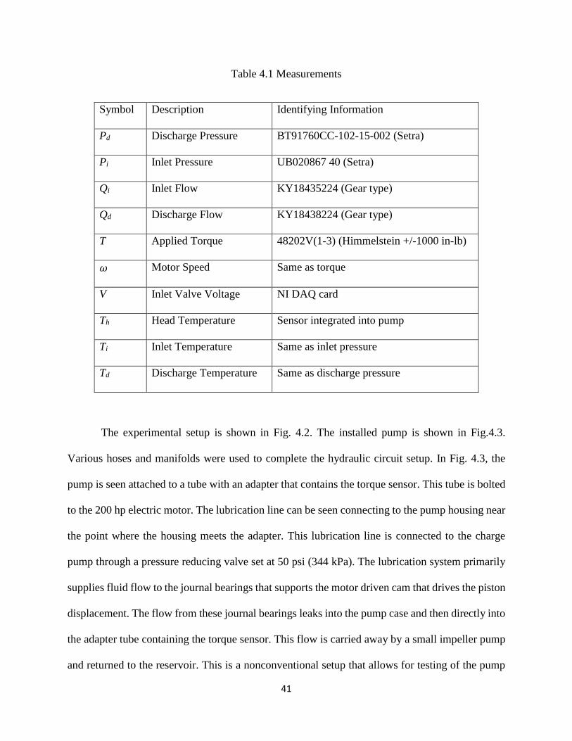
Table 4.1. Measurements ................................................................................................. 41
Table 2. Data collection points associated with experiments .......................................... 44
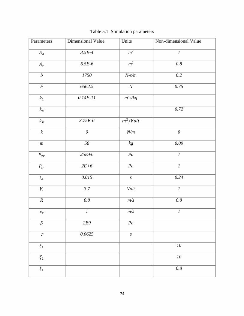
Table 5.1. Simulation parameters .................................................................................... 73
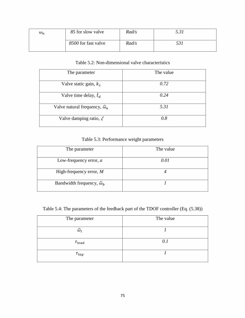
Table 5.2. Non-dimensional valve characteristics .............................................................. 74
Table 5.3. Performance weight parameters ........................................................................ 75
Table 6. The parameters of the feedback part of the TDOF controller (Eq. (5.38)) ............. 75
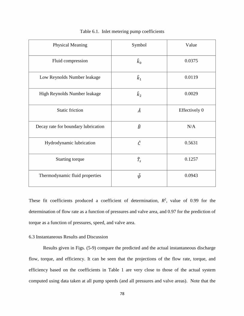
Table 7. Inlet metering pump flow and torque coefficients ............................................. 78
Page 13
xii
NOMENCLATURE
A Static Friction Coefficient
𝐴𝐴 Actuator Cross Sectional Area
Ap Cross-Sectional Area of the Piston Pump
Av Valve Opening Area
a Maximum Low Frequency Error
B Boundary Lubrication Decay Rate Coefficient
C Hydrodynamic Lubrication Coefficient
e Steady State Error
F Disturbance Force
𝐹𝑜 Spring Preload
G Plant Transfer Function
Gv Valve Transfer Function
K H∞ Controller Transfer Function
k Spring Stiffness Coefficient
k0 Fluid Compression Coefficient
k1 Low Reynolds Number Leakage
k2 High Reynolds Number Leakage
𝐾𝑑 Derivative Controller Gain
𝐾𝑝 Proportional Controller Gain
l Width of the Camshaft Journal Bearing
m Mass of the Working Fluid within the Piston Volume
Π Hydraulic Power
Page 14
xiii
P Pressure
P Generalized Plant
Q Volumetric Flow Rate
r Camshaft Radius
S Sensitivity
T Total Torque on the Camshaft
T Closed-Loop Transfer Function
Tc Torque Required to force the Air out of the solution and Condense the vaporized
fluid
Temp Temperature
Tf Friction Torque
Tideal Ideal Torque
Tref Desired Closed-Loop Transfer Function
Ts Starting Torque
V Voltage
Vd Volumetric Displacement of the Pump
𝑉𝑜 Actuator Volume
Vout Valve Feedback Voltage
W load per unit length
wp Performance weight
wu Controller Effort Weight
α Swashplate Angle
Page 15
xiv
β Fluid Bulk Modulus
η Overall Pump Efficiency
ηa Actuator Efficiency
µ Fluid Viscosity
µs Friction Coefficient
τlag Lag Time Constant
τlag Lag Time Constant
ω Pump Shaft Speed
ωI Zero Location of the Integral Controller
ωn Natural Frequency
ωb Bandwidth Frequency
𝜓 Parameter for thermodynamic fluid properties
𝜏 Time Constant
𝜉 Damping Ratio of the Valve
𝜉1 Nondimensional Group
𝜉2 Nondimensional Group
SUBSCRIPTS
A Port A of the actuator
B Port B of the actuator
d Discharge
i inlet
l Leakage
r Reference Conditions
Page 16
xv
SUPERSCRIPTS
^ Nondimensional Quantity
Averaged Quantity
Page 17
xvi
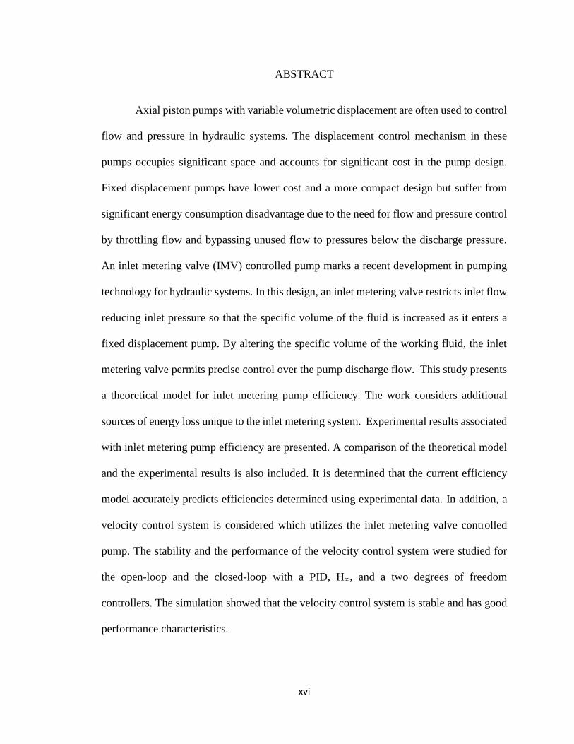
ABSTRACT
Axial piston pumps with variable volumetric displacement are often used to control
flow and pressure in hydraulic systems. The displacement control mechanism in these
pumps occupies significant space and accounts for significant cost in the pump design.
Fixed displacement pumps have lower cost and a more compact design but suffer from
significant energy consumption disadvantage due to the need for flow and pressure control
by throttling flow and bypassing unused flow to pressures below the discharge pressure.
An inlet metering valve (IMV) controlled pump marks a recent development in pumping
technology for hydraulic systems. In this design, an inlet metering valve restricts inlet flow
reducing inlet pressure so that the specific volume of the fluid is increased as it enters a
fixed displacement pump. By altering the specific volume of the working fluid, the inlet
metering valve permits precise control over the pump discharge flow. This study presents
a theoretical model for inlet metering pump efficiency. The work considers additional
sources of energy loss unique to the inlet metering system. Experimental results associated
with inlet metering pump efficiency are presented. A comparison of the theoretical model
and the experimental results is also included. It is determined that the current efficiency
model accurately predicts efficiencies determined using experimental data. In addition, a
velocity control system is considered which utilizes the inlet metering valve controlled
pump. The stability and the performance of the velocity control system were studied for
the open-loop and the closed-loop with a PID, H∞, and a two degrees of freedom
controllers. The simulation showed that the velocity control system is stable and has good
performance characteristics.
Page 18
1
CHAPTER 1
INTRODUCTION
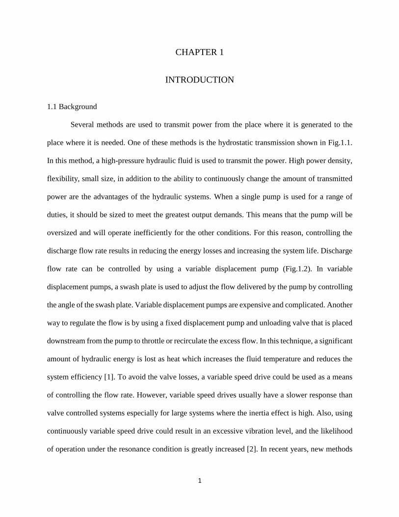
1.1 Background
Several methods are used to transmit power from the place where it is generated to the
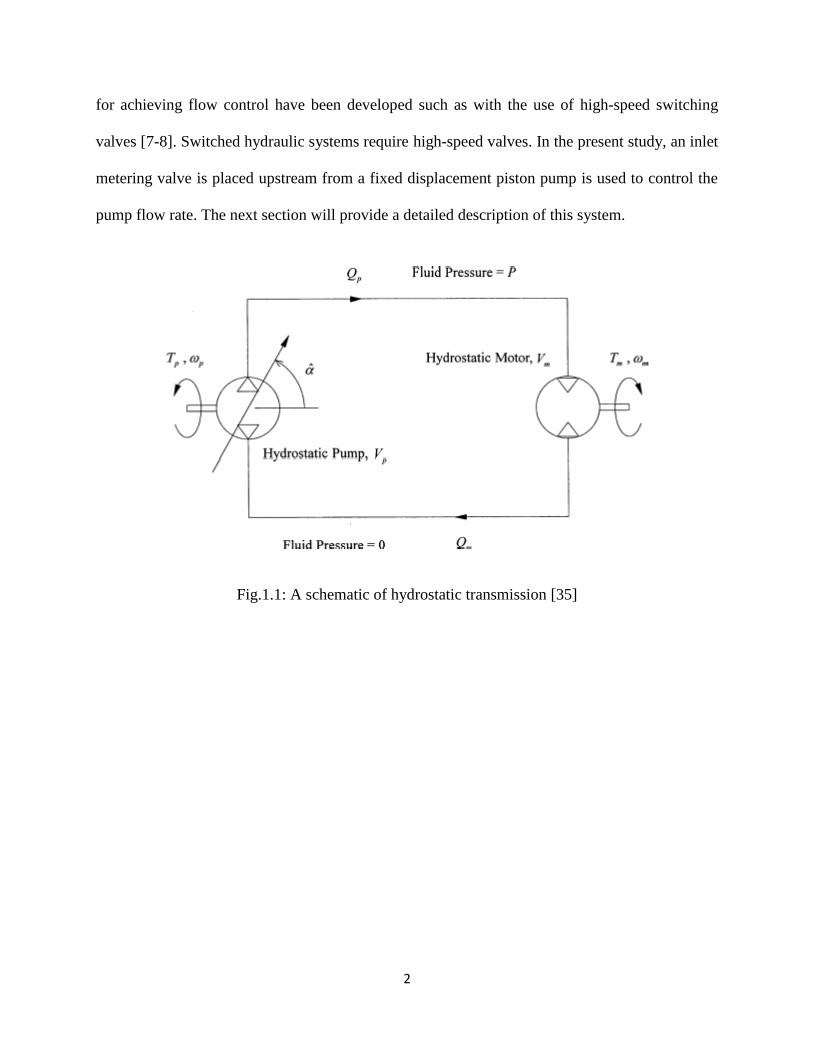
place where it is needed. One of these methods is the hydrostatic transmission shown in Fig.1.1.
In this method, a high-pressure hydraulic fluid is used to transmit the power. High power density,
flexibility, small size, in addition to the ability to continuously change the amount of transmitted
power are the advantages of the hydraulic systems. When a single pump is used for a range of
duties, it should be sized to meet the greatest output demands. This means that the pump will be
oversized and will operate inefficiently for the other conditions. For this reason, controlling the
discharge flow rate results in reducing the energy losses and increasing the system life. Discharge
flow rate can be controlled by using a variable displacement pump (Fig.1.2). In variable
displacement pumps, a swash plate is used to adjust the flow delivered by the pump by controlling
the angle of the swash plate. Variable displacement pumps are expensive and complicated. Another
way to regulate the flow is by using a fixed displacement pump and unloading valve that is placed
downstream from the pump to throttle or recirculate the excess flow. In this technique, a significant
amount of hydraulic energy is lost as heat which increases the fluid temperature and reduces the
system efficiency [1]. To avoid the valve losses, a variable speed drive could be used as a means
of controlling the flow rate. However, variable speed drives usually have a slower response than
valve controlled systems especially for large systems where the inertia effect is high. Also, using
continuously variable speed drive could result in an excessive vibration level, and the likelihood
of operation under the resonance condition is greatly increased [2]. In recent years, new methods
Page 19
2
for achieving flow control have been developed such as with the use of high-speed switching
valves [7-8]. Switched hydraulic systems require high-speed valves. In the present study, an inlet
metering valve is placed upstream from a fixed displacement piston pump is used to control the
pump flow rate. The next section will provide a detailed description of this system.
Fig.1.1: A schematic of hydrostatic transmission [35]
Page 20
3
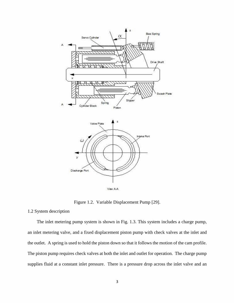
Figure 1.2. Variable Displacement Pump [29].
1.2 System description
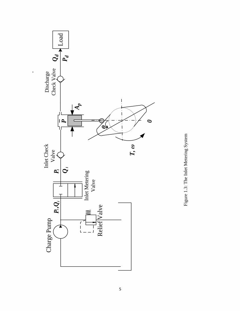
The inlet metering pump system is shown in Fig. 1.3. This system includes a charge pump,
an inlet metering valve, and a fixed displacement piston pump with check valves at the inlet and
the outlet. A spring is used to hold the piston down so that it follows the motion of the cam profile.
The piston pump requires check valves at both the inlet and outlet for operation. The charge pump
supplies fluid at a constant inlet pressure. There is a pressure drop across the inlet valve and an
Page 21
4
increase in volume in the space between the valve and the pump piston as the piston moves
downward. This increase in volume results in some combination of partial vaporization of the oil
and dissolved air coming out of solution with the oil.
As the pump operates, the volume trapped between the inlet valve and the piston increases
and the fluid pressure, P, decreases causing the check valve to open. In the volume between the
inlet valve and the piston, the fluid partially vaporizes or dissolved air to comes out of the solution
effectively increasing the specific volume of the fluid. Fluid accumulates upstream from the first
check valve. As the line upstream from the check valve is filled, the check valve opens and the
piston volume fills with the liquid/gas/vapor mixture. This occurs when the piston is in the bottom
dead center position. As the camshaft rotates, it forces the piston head upwards. The size of the
internal piston volume decreases, which results in an elevated pressure and closing of the inlet
check valve. The increased pressure condenses the fluid and forces the trapped air back into
solution. After the fluid pressure reaches a pressure of Pd the second check valve opens and the
fluid travels downstream at a flow rate of Qd. Then the second check valve closes as the cylinder
pressure decreases when the piston moves downward and the process continues with new fluid
entering the control volume.
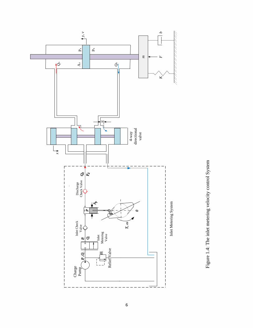
1.3 Velocity control system
The velocity control system for a linear actuator that utilizes an inlet metering system is shown in
Figure 1.4. The system consists of an inlet metering system, a four-way directional valve, and a
linear actuator. The four-way directional valve is always wide open to one of the actuator ports. It
is used to guide the flow of the inlet metered pump (IMP) to one of the actuator ports, as required,
according to the desired direction of the velocity of the hydraulic cylinder. The flow from the other
port of the actuator is returned to the tank through the four-way directional valve.
Page 22
5
iP
,Qi
Ch
arg
e P
um
p
Rel
ief
Val
ve
T,
ω
Pd
Qd
Ap
P
1
1
P 0
Ѳ
Inle
t C
hec
k
Val
ve
Dis
char
ge
Ch
eck
Val
ve
Q
Inle
t M
eter
ing
Val
ve
Lo
ad
Fig
ure
1.3
: T
he
Inle
t M
eter
ing S
yst
em
Page 23
6
4-w
ay
dir
ecti
on
al
val
ve
Inle
t M
eter
ing
Sy
stem
iP,Q
i
Ch
arg
e
Pu
mp R
elie
f V
alv
e
T,
ω
Pd
Qd
Ap
P
1
1
P 0
Ѳ
Inle
t C
hec
k
Val
ve
Dis
char
ge
Ch
eck
Val
ve
Q Inle
t
Met
erin
g
Val
ve
x
m
PA
PB
QA
QB
FK
u
AA
y, v b
Fig
ure
1.4
: T
he
inle
t m
eter
ing v
eloci
ty c
ontr
ol
Sy
stem
Page 24
7
1.4 Contributions of the present work
The main objective of this work is to make an assessment of the feasibility of using an inlet
metering pump within standard hydraulic circuits to replace axial piston pumps by conducting tests
and analysis of performance and efficiency. The specific objectives are as follows:
1. Create a model of the inlet metered pump to determine its theoretical performance and to
understand the physical phenomena involved in the pump dynamics and performance.
2. Test the inlet metered pump in the lab to determine the performance of the pump in terms of
efficiency and to validate the model.
3. Analyze test data and model so that we can make conclusions about the performance of the
pump and feasibility of using the pump in hydraulic systems.
4. Disassemble the pump after testing to search for any signs of significant wear possibly due to
cavitation.
5. Make recommendations about the future use of the inlet metering system concept.
6. Design a velocity control system that utilizes the inlet metering system.
1.5 Dissertation outline
This dissertation is divided into seven chapters. Chapter one presents a background on flow
control techniques and a description of the inlet metering system with an application on the
hydraulic control systems. In chapter two, works carried out by other researchers on the flow
control methods are reviewed and discussed. The analysis and modeling of the inlet metered pump
flow, torque and efficiency are developed in chapter three. This chapter also presents the way of
nondimensionalization of the model. The experimental setup details and the test conditions are
described in chapter four. Chapter five presents the design of the inlet metering velocity control
system. Open-loop and closed-loop analysis are also discussed in this chapter. The validation of
Page 25
8
the model and the results from the experimental and theoretical analysis are presented in chapter
six. Finally, a list of conclusions from this work followed by some recommendations for future
work is presented in chapter seven.
Page 26
9
CHAPTER 2
LITERATURE REVIEW
2.1 Introduction
This chapter aimed at providing an overview of the available literature that is relevant to
this study. It reviews various ways that are used to control the flow rate of a pump using variable
and fixed displacement pumps. Due to the similarity between the inlet metering system and the
fuel injection system in the diesel engines, a review of the published studies for the diesel injector
system will also be presented in this section. A review of available literature on cavitation
phenomenon is also presented in this chapter to provide a good understanding of this phenomenon
that might be associated with the inlet metering systems. The chapter ends with a summary of the
reviewed literature.
2.2 Variable displacement pumps
Many investigations have been done to design and analyze the variable displacement
machines. Displacement controlled systems are energy efficient [3]. Wilson [4] developed a model
for volumetric and torque efficiencies. His model included viscous torque and low Reynolds
number leakage equations. The high Reynolds number leakage was taken into account by the
model developed by Schlosser [5]. In order to extend the previous model to include the variable
displacement machines, Thoma [6] developed a model introducing the frictional coefficient.
Equations for the swash plate dynamic were derived and written in a linearized form in the model
developed by Aker and Zeiger [7]. The effect of oil entrapment behind the valve plate was studied
by Aker and Zeiger [8]. They discussed the effect of swashplate angle, pump speed, and discharge
pressure, in addition to the entrapment angle on instantaneous pressure and torque by solving the
Page 27
10
dynamical equations of motion. In their analysis, they divided the pressure distribution into six
regions depending on the angular position of the piston. Their results showed that the peak
pressures vary as the pump angular speed or the swashplate angle varies. The entrapment angle
was shown to have no effect on the peak pressure, but it affects the pressure recovery time and the
torque.
Kaliafetis and Th. Costopoulos [9] studied the characteristics of a standard variable
displacement axial piston pump with a pressure regulator. They derived the governing equations
for the system and used computer simulation to determine the parameters that affect the pump
operating pressure. Their results were compared with the manufacturer’s curve and showed good
agreement. They concluded that the outlet pressure is mainly affected by the control valve position
which affects the piston pressure and on the pistons areas.
Closed form equations that may be used for a variable displacement design were provided
in a study developed by Manring and Johnson [10]. They discussed the effect of changing the
volume of the actuator and the hose, the controller flow gain, and the leakage. In their model, they
assumed that the inertia and damping of the swash plate are negligible compared to the stiffness
of the control actuator.
The damping mechanism on the swashplate that is caused by the piston pressure was
studied by Zhang et al. [11] by assuming a pressure profile for a variable swashplate angle. A
linearized model of the hydrostatic transmission with details of the pump dynamics was developed
by Manring, N.D. and Luecke, G.R [12] which does not need to use experimental data -- the
modeling parameters may be determined from the geometry of the transmission. A third order
system was produced from the dynamics of the pump, the motor, and the hose. The stability of the
system was discussed using the Routh-Hurwitz criterion.
Page 28
11
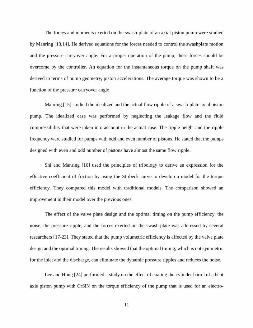
The forces and moments exerted on the swash-plate of an axial piston pump were studied
by Manring [13,14]. He derived equations for the forces needed to control the swashplate motion
and the pressure carryover angle. For a proper operation of the pump, these forces should be
overcome by the controller. An equation for the instantaneous torque on the pump shaft was
derived in terms of pump geometry, piston accelerations. The average torque was shown to be a
function of the pressure carryover angle.
Manring [15] studied the idealized and the actual flow ripple of a swash-plate axial piston
pump. The idealized case was performed by neglecting the leakage flow and the fluid
compressibility that were taken into account in the actual case. The ripple height and the ripple
frequency were studied for pumps with odd and even number of pistons. He stated that the pumps
designed with even and odd number of pistons have almost the same flow ripple.
Shi and Manring [16] used the principles of tribology to derive an expression for the
effective coefficient of friction by using the Stribeck curve to develop a model for the torque
efficiency. They compared this model with traditional models. The comparison showed an
improvement in their model over the previous ones.
The effect of the valve plate design and the optimal timing on the pump efficiency, the
noise, the pressure ripple, and the forces exerted on the swash-plate was addressed by several
researchers [17-23]. They stated that the pump volumetric efficiency is affected by the valve plate
design and the optimal timing. The results showed that the optimal timing, which is not symmetric
for the inlet and the discharge, can eliminate the dynamic pressure ripples and reduces the noise.
Lee and Hong [24] performed a study on the effect of coating the cylinder barrel of a bent
axis piston pump with CrSiN on the torque efficiency of the pump that is used for an electro-
Page 29
12
hydraulic actuator. The pump in these systems exhibits unsteady conditions because it operates
only when error compensation is needed. These unsteady conditions cause wear on the valve plate.
Their results showed that the coated cylinder barrel has much lower friction coefficient compared
to the original cylinder. The friction coefficient of the coated cylinder was shown to be independent
of the normal load while it is proportional to the normal load in case of the original cylinder. An
improvement of 1.3 percent in the torque efficiency was achieved by coating the cylinder barrel.
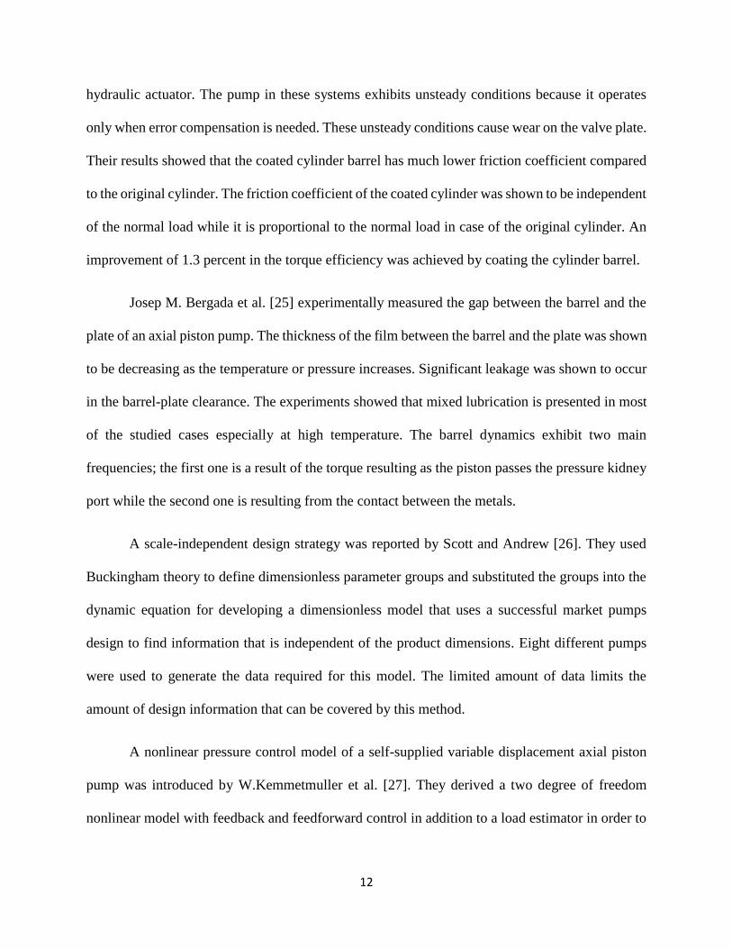
Josep M. Bergada et al. [25] experimentally measured the gap between the barrel and the
plate of an axial piston pump. The thickness of the film between the barrel and the plate was shown
to be decreasing as the temperature or pressure increases. Significant leakage was shown to occur
in the barrel-plate clearance. The experiments showed that mixed lubrication is presented in most
of the studied cases especially at high temperature. The barrel dynamics exhibit two main
frequencies; the first one is a result of the torque resulting as the piston passes the pressure kidney
port while the second one is resulting from the contact between the metals.
A scale-independent design strategy was reported by Scott and Andrew [26]. They used
Buckingham theory to define dimensionless parameter groups and substituted the groups into the
dynamic equation for developing a dimensionless model that uses a successful market pumps
design to find information that is independent of the product dimensions. Eight different pumps
were used to generate the data required for this model. The limited amount of data limits the
amount of design information that can be covered by this method.
A nonlinear pressure control model of a self-supplied variable displacement axial piston
pump was introduced by W.Kemmetmuller et al. [27]. They derived a two degree of freedom
nonlinear model with feedback and feedforward control in addition to a load estimator in order to
Page 30
13
achieve a solution for the unknown variable load. Lyapunov’s theory was used in their model to
determine the system stability. Their results proved the robustness of the control model.
A study that performed by Zhiru et al. [28] examined the flow ripple generated in an axial
piston pump in a similar way that was done by Manring [15] but for conical barrel design. They
concluded that the flow ripple depends on the swashplate angle and the conical barrel angle. The
conical barrel pump was shown to have a slight increase in the output flow and decrease in the
inertia compared the cylindrical barrel pump under the same operating conditions. The frequency
analysis showed an additional order which caused undesired noise and vibration.
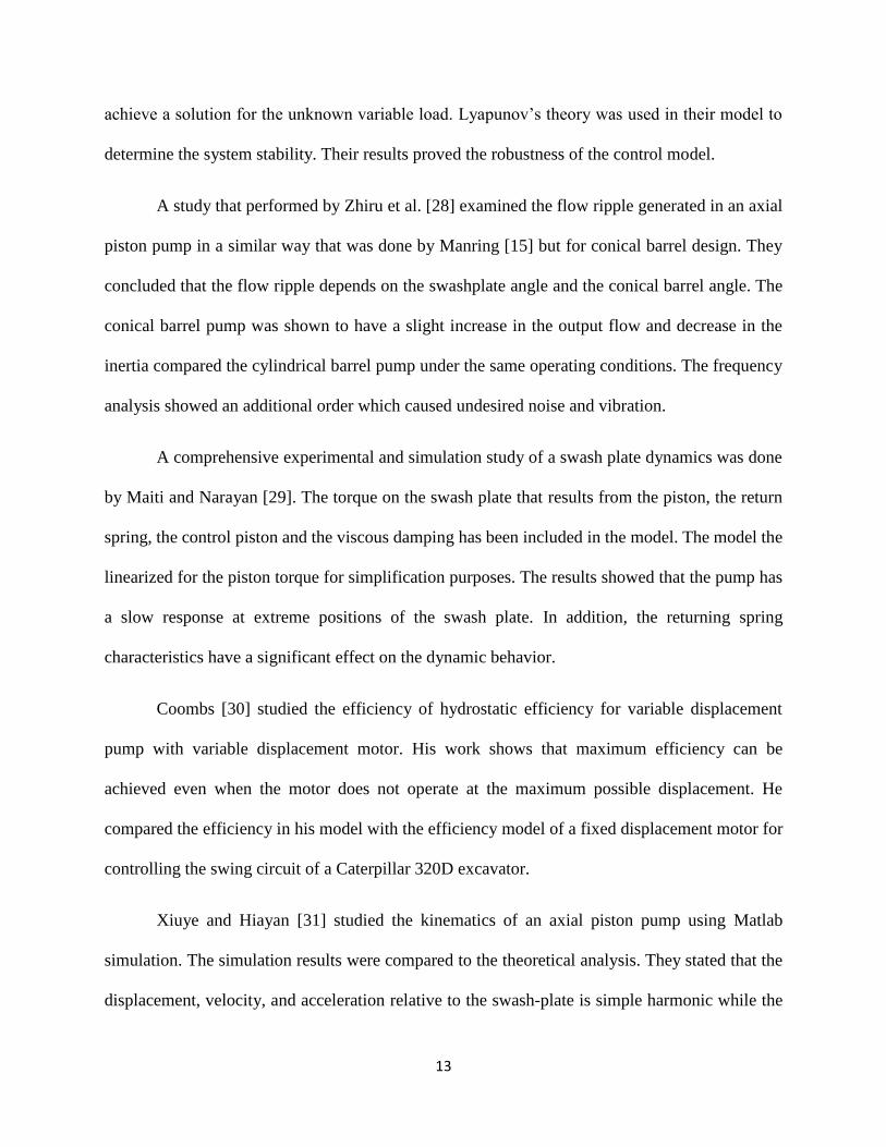
A comprehensive experimental and simulation study of a swash plate dynamics was done
by Maiti and Narayan [29]. The torque on the swash plate that results from the piston, the return
spring, the control piston and the viscous damping has been included in the model. The model the
linearized for the piston torque for simplification purposes. The results showed that the pump has
a slow response at extreme positions of the swash plate. In addition, the returning spring
characteristics have a significant effect on the dynamic behavior.
Coombs [30] studied the efficiency of hydrostatic efficiency for variable displacement
pump with variable displacement motor. His work shows that maximum efficiency can be
achieved even when the motor does not operate at the maximum possible displacement. He
compared the efficiency in his model with the efficiency model of a fixed displacement motor for
controlling the swing circuit of a Caterpillar 320D excavator.
Xiuye and Hiayan [31] studied the kinematics of an axial piston pump using Matlab
simulation. The simulation results were compared to the theoretical analysis. They stated that the
displacement, velocity, and acceleration relative to the swash-plate is simple harmonic while the
Page 31
14
piston moves in an elliptic trajectory relative to the swash-plate. They also reported that the
instantaneous pump flow rate is depending on the piston motion which is affected by the
swashplate angle.
Manring [32] developed a complete model for the overall efficiency of hydrostatic
transmission for variable displacement pump and motor. More recently, Manring et. al. [33]
discussed the speed limitations of an axial piston machines. The first perspective that was studied
was the Cylinder block tipping which occurs as a result of operating under the conditions of low
pressure, high displacement, or high speed. These conditions occur when the cylinder-block spring
fails to counteract imbalance of centrifugal inertial effects as a result of the piston reciprocation
and try to separate the cylinder block from the valve plate resulting in a fluid seal between them.
The second perspective that was investigated was the cylinder block filling. It occurs at high-speed
operation when the cylinder is filled partially with fluid vapor. The last perspective studied in this
study was the slipper tipping which means separating the piston from the slipper as a result of the
tensile force that is generated as the piston starts the transition from the discharge to the inlet port
caused by the same conditions that cause the cylinder block tipping. All the speed limitations were
scaled by the inverse cube root of the volumetric displacement of the original machines. New
machines were produced by using the scale laws which were shown to be identical for the three
speed limitations.
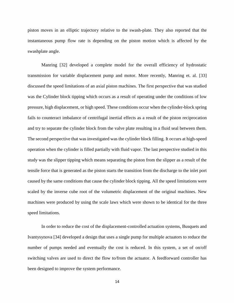
In order to reduce the cost of the displacement-controlled actuation systems, Busquets and
Ivantysynova [34] developed a design that uses a single pump for multiple actuators to reduce the
number of pumps needed and eventually the cost is reduced. In this system, a set of on/off
switching valves are used to direct the flow to/from the actuator. A feedforward controller has
been designed to improve the system performance.
Page 32
15
Manring [35] has developed a model to generate an efficiency maps for hydrostatic
transmission. His model was similar to his previous model [32] with some modifications
concerning the input torque where the friction torque was divided into two parts, the side load
within the machine and the normal load. The results that were presented in a nondimensional form
showed that the efficiency is nearly independent of neither the output torque nor the speed under
certain operating conditions.
2.3 Fixed displacement pumps
Generating a variable flow source using a fixed displacement pump and unloading valve
was studied by several researchers [36,37]. They presented a way in which a variable flow source
is achieved using a fixed displacement pump and unloading valve downstream from the pump. In
addition to the low cost and the complexity of this system, it has a longer life compared to the
variable displacement pump because the pump in this system is unloaded under zero flow
condition which reduces the force exerted on the pump under zero or low flow conditions. They
studied the losses resulted from switching power, compressing and decompressing the oil, and the
metering when switch pumping between the system and the tank. Their results showed that the
main losses were due to transition during the valve opening and closing. It is also shown that
switching the unloading valve on and off does not cause the pump to be shock loaded.
A velocity control system for a linear actuator using a feedforward plus PID (FPID)
controller was designed by Zhang [38]. In this design, the flow is controlled using directional
throttling valve. The system nonlinearity was compensated by the feedforward loop while the
velocity tracking error was compensated by the PID controller. The results show that the R-squared
resulted from the FPID controller is 15% lower than that resulted from the feedforward loop and
45% lower than that from the PID controller. The results also show that using the FPID controller
Page 33
16
improves the stability and the performance of the system. Variable flow can also be generated
using a variable speed fixed displacement pump.
Gibson [39] introduced a method of determining the flow of a variable speed centrifugal
pump using the flow/head characteristics of the pump. The results showed that for high static head
conditions, the head is very sensitive to the speed and requires less than five percent speed variation
to cover the whole flow rate range.
Çalişkan, H., et al. [1] studied a position control of a hydraulic system using a variable
speed drive to control the flow according to the system requirements. Kalman filter was applied
for noise reduction in the feedback signal. The model outputs were compared to open loop and
closed loop frequency and step response to depict the dynamic performance of the system. The
losses of this system were compared to the losses of the valve controlled hydraulic system. They
stated that only 38.5% of the power produced by the pump could be transmitted to the system in a
valve controlled hydraulic system.
Hu et al. [40] conducted simulation and experimental study to control the load velocity for
a hydraulic system using variable speed drive. They used a compound algorithm to meet the system
requirements. The compound algorithm consists of PD-controller and feedforward-feedback
control. The experiments were performed on a hydraulic elevator test rig. They studied the transfer
function and frequency-domain of the system. The results showed that the frequency and damping
of the large inertia hydraulic speed-control system are low. They also stated there is a steady-state
error of velocity when using unity-feedback control without compensation.
An approach for controlling pressure using an inlet metering pump, which uses a fixed
displacement pump to provide a variable flow for a water hydraulic system, was introduced by
Page 34
17
Wisch [41]. A nondimensional analytical model was developed that relates the inlet metering valve
opening to the discharge flow of the pump. The pressure was shown to exhibit a first order
response.
2.4 Switched systems
Brown [42] introduced a new technique of controlling system flow rate or the pressure
using a switched inertance device. In this technique, the flow is controlled using an extremely fast
valve to switch the flow between the tank and the load. For simplicity, it was assumed that the
valve switches instantaneously in this study. An experimental study on the design of a rotary fluid
switch that is needed to accomplish the required pulse-width modulation at a high frequency is
developed by Brown et al. [43]. The efficiency of the rotary valve was shown to be higher than
that of the standard servo valve for moderate flow conditions. The study stated that a design of the
tank-side chamber with air pockets reduces the cavitation associated with these systems.
Johnston et al. [44] presented an experimental and simulation study on a switched inertance
hydraulic system for flow and pressure control in a way that is similar to an electrical switched
inductance. They studied two modes of switched inertance hydraulic system which are flow and
pressure boosters by changing the connections at the inlet and outlet of the system. The results
showed that using a switched inertance system could provide flow and pressure less or more than
the inlet flow and pressure respectively as required. The results also showed that the four-port
design of the of the switched inertance system better control characteristics and higher efficiency
than a four-port closed-center valve.
In order to meet the requirement of the high switching frequency of the switched inertance
system, a high-speed rotary valve has been introduced by Pan [45]. They experimentally studied
the characteristics of the rotary valve for the steady state and dynamic conditions. The effect of the
Page 35
18
frequency and switching ratio on the pressure, flow, and the efficiency has been studied. The
results showed that under the optimal frequency conditions, the efficiency increases as the
switching ratio increases. They stated that the inertance switching system has a promising
performance.
The problem of noise associated with these systems was discussed in a study developed by
Pan et al. [46]. In this study, a controller, that uses a flow booster with a bypass was designed for
the purpose of canceling the pressure pulsation that causes the noise. The results showed that using
this design can reduce the pressure pulsation. It was also shown that increasing the booster size
reduces the noise. However, of the frequency, flow and pressure are limited due to the limitations
of the hardware.
Scheidl et al. [47] developed a model for a hydraulic buck converter using time-frequency
domain simulation. The time domain has been applied to switching and check valves while the
frequency domain has been applied to the pulsating waves in the pipe. The complexity of the check
valve behavior was reduced by replacing the valve pressure and flow rate with a single variable
which generated a system of nonlinear equations. The system of the nonlinear equations was
solved using Newton-Raphson algorithm.
Pan et al. [48] developed an analytical model for three-port switched inertance system
using lump and distributed parameter models. The efficiency and performance of the system were
studied. The system efficiency was modeled as a function of delivery flow rate, flow loss,
resistance, and the pressure difference. The results showed that the pressure loss increases as the
delivery flow increases.
Page 36
19
To improve the estimation of the system efficiency and the accuracy of the system
dynamics modeling, Pan et al. [49] developed an enhanced model the includes the valve dynamics,
leakage, and nonlinearity. The model was also validated against experiments. The results of the
improved model showed that the flow loss increases as the delivery flow increases. It was also
shown that the flow loss associated with the enhanced model is greater than those associated with
the original basic model.
2.3 Fuel injection systems
Since the inlet metering pump uses similar principles of the fuel injection systems, a review
of some of the available literature on the fuel injection systems and the cavitation associated with
it is found in this section. The problem of vibration and noise resulted from the fuel pressure
pulsation in the fuel injection system was treated by the experimental research that was done by
Ito, and Miyoshi [50]. In this steady, a damper was used to avoid what is called “water hammer
phenomenon’’ in the pipes leading the fuel to the engine that is caused by the excessive fuel
pressure variation.
Miyaki, M. et al. [51] developed a design for electronically controlled common rail
injection system called ECD-U2 system that is capable of controlling the fuel quantity and pressure
independently. The system operates at 120MPa. The flow out of the high-pressure pump is
controlled a pressure control valve which, accordingly, controls the rail pressure. A three-way
valve was designed to adjust the nozzle back pressure to control the nozzle lift. A simpler design
was conducted by Rinolfi, R. et al. [52] using a two-way solenoid valve instead of the three-way
valve in the previous design to control the fuel injection. Detailed design of the two-way solenoid
two-way valve was developed by Stumpp, and Ricco [53]. In this design, the flow of the radial
piston high-pressure pump is controlled by the two-way solenoid valve.
Page 37
20
A new design of a common rail fuel injection system for a high pressure that is up to
160Mpa and a wide range of engine speed was developed by Guerrassi, et al. [54] which is called
Locus Diesel Common Rail system. The system consists of a high-pressure pump, rail, injectors,
in addition to an electronic control unit. The pump pressure is controlled by a pressure control
valve while the fuel quantity is controlled by an inlet metering valve. This design provides engine
stability improvement in addition to the ability to use multiple injections each stroke.
A comprehensive model of the vaporization process of the fuel at high pressure was
introduced by Zhu and Reitz [55]. The continuous thermodynamic concepts were used to consider
the effect of the high pressure on the vaporization process of the fuel droplet in the gas and diesel
engines. The effect of fuel type was also studied. Furthermore, the study investigated the influence
of using two components fuel and compared the results to the single component fuel case. The
results showed that there is a significant effect of using multicomponent fuel on the system
performance, especially for high volatility fuels.
Balluchi et al. [56,57] developed a hybrid model to control the rail pressure for the common
rail injection systems. The model was compared to the one based on the mean value, and it was
shown to have better performance. The model also can handle the delay and the interaction
between the system components. In addition, the high-pressure pump efficiency was studied and
was shown to be proportional to the discharge pressure.
Ryu et. al. [58] investigated the cavitation phenomena in a fuel injection pump during the
process of fuel delivery using optical visualization method. They used twelve pumps with different
parts geometries in the study. Two types of cavitation were observed. The first type is a fountain-
like cavitation that occurs before the end of the fuel delivery, and it causes a plunger damage. The
second type is a jet cavitation which occurs after the spill end, and it causes a barrel damage. Their
Page 38
21
results showed that cavitation could be reduced by decreasing the area of the perpendicular impact
with the jet. This can be achieved by using a conical spill port.
The problem of fuel evaporation in the injection systems for the small engines, in which
the injector acts as a pump, was dealt with by the study conducted by Allen, et al. [59]. This design
provides escaping path for the fuel vapor from the injector to the fuel tank. The injector in this
design is immersed in the fuel so that the flow restrictions are reduced by getting rid of the injector
casing which improves the efficiency of the system.
While the traditional fuel metering systems consist of pumping device and metering valve,
a study conducted by Schwamm, [60] aimed to reduce the complexity of the fuel metering system
in aero engines by either controlling the pump speed electronically and getting rid of the metering
device or reducing the complexity of the valve itself. The study results showed that this modified
design has higher performance, faster response, and 20-40% lower cost than the traditional
systems.
The effect of the nozzle geometry, injection pressure and back pressure on the cavitation
in a diesel injection system was studied experimentally and numerically by He, et al. [61]. Quasi-
Newton and Universal Global Optimization methods were used to predict a correlation between
the cavitation number and the critical conditions at which the cavitation starts. It was found that
the discharge coefficient is proportional to the cavitation number.
Duan et al. [62] developed a new design of a fuel injection system by adding control
orifices that are adjusted by a control piston in order to develop a system with a fast response. The
new system performance was compared to that of the conventional one. The nonlinear cavitation
model was used with a dynamic grid to study the cavitation associated with both systems
Page 39
22
numerically using CFD technique. Then, the numerical results were compared with the
experimental results for the validation purpose.
2.6 Cavitation
Cavitation is a Phenomenon that has a strong impact on hydraulic characteristics in
hydraulic machines [63]. It happens when the liquid pressure drops below the vapor pressure [64].
Cavitation damage is caused by bubbles collapsing near the surface [65]. Wang [66] studied the
cavitation phenomena the axial piston pumps. The study included optimization of the valve plate
design in order to reduce the cavitation. The optimization was accomplished by modifying the
geometry of the valve plate so that enough fluid flows into the piston internal volume to keep the
pressure higher than the vapor pressure. Analytical relationship has been developed that relates the
cavitation to the valve plate geometry. The results showed that the cavitation increases as the
pumping speed increases.
Many researchers have studied the cavitation resistance of materials and recommended
different cavitation resistant materials. Ceramic has been shown to have good cavitation resistance
[67 and 68]. CrB2 was also found to have excellent corrosion resistance properties [69].
Poliarus, et al. [70] experimentally studied the corrosion and cavitation wear resistance of
new composites based on NiAl and NiTi. The new composites may be used in hydropower
equipment that are exposed to aggressive environments and cavitation conditions. The results
showed that the new composite (NiTi-30wt.% CrB2) has better cavitation resistance than NiTi.
The dynamics of the cavitation bubbles interaction in an acoustic field was studied by
Liang et al. [71] using a sonication recording system. In addition, the cavitation bubbles interaction
dynamics was studied theoretically using Keller-Miksis model. Both the experimental and
Page 40
23
theoretical results showed that the cavitation bubbles interaction plays a major role in the cavitation
bubbles dynamics. The results also showed that the bubble sizes have a strong effect on interacting
bubbles oscillation.
Wang et al. [72] investigated the effect of filling the defects in carbon steel coated by 8
wt.% yttria stabilized zirconia with epoxy on the cavitation resistance. The results showed that
filling the cavities of the coating with epoxy greatly improves the cavitation resistance. A
comparison study of cavitation resistance was performed by Bordeasu et al. [73]. Cavitation
resistance of steel with different content of carbon (0.03% - 0.1%), chromium (2%-24%) and
nickel (0.5%-10%) was tested. The results showed that steel with the content of 0.1% carbon, 12%
chromium and 6% nickel has the best cavitation resistant properties in the studied range.
2.7 Literature Review Summary
Numerous studies have been done on providing a variable flow source that has high
efficiency, good performance, and low cost. Different techniques have been studied to meet those
requirements. Although variable displacement pumps are efficient and have good performance,
they are expensive and complicated. On the other hand, traditional valve controlled systems are
less expensive because they use fixed displacement pumps. However, the energy dissipated, as
heat, that is associated with these systems is high due to the high pressure drop across the valve.
Variable speed drive is another option that is used to achieve variable flow. For large systems, the
inertia effect is high which limits the speed of the response of these systems. Recently, inertance
tube switch systems have been studied as an alternative flow control technique. Noise and flow
ripple are problems that are associated with these systems. Switched systems also require
extremely fast valves to switch the flow between the tank and the load.
Page 41
24
In this work, a new flow control technique was studied and analyzed. The new technique
uses an inlet-metering valve to manipulate the flow of a piston pump in a way similar to the inlet
metering system in the fuel injection systems. This work builds on previous analytical work [41]
aimed at modeling and analysis of an inlet metering pump used in a pressure control system. The
pump used in this system is fixed displacement pump which reduces the cost and complexity of
the system. Since the inlet metering valve is placed upstream from the pump, the energy dissipated
across the valve is minimized due to the arbitrarily small pressure drop. In addition, the inlet-
metering system has good performance and does not require an extremely fast valve. Models for
the flow, torque, and efficiency of this system have been developed in this study and validated
against experimental data collected from an experimental setup. A design of a velocity control
system that utilizes the inlet metering system was also a part of this work. Due to the fluid
vaporization associated with this system, a cavitation problem may exist. Cavitation resistant
material may be used to build the parts that might be exposed to cavitation conditions as suggested
by the literature. However, studying the cavitation phenomenon is beyond the scope of this work.
Page 42
25
CHAPTER 3
INLET-METERED PUMP EFFICIENCY
3.1 Introduction
A general definition of the machine efficiency is the ratio of output power to the input
power. The overall efficiency of the system is a combination of the volumetric efficiency and the
mechanical efficiency. The volumetric efficiency is a measure of the flow losses while the
mechanical efficiency is a measure of the torque losses. The flow loss is a combination of
compressibility loss, low Reynolds number loss, and high Reynolds number loss. The torque losses
consist of frictional loss, starting torque loss and the torque associated with the vaporization and
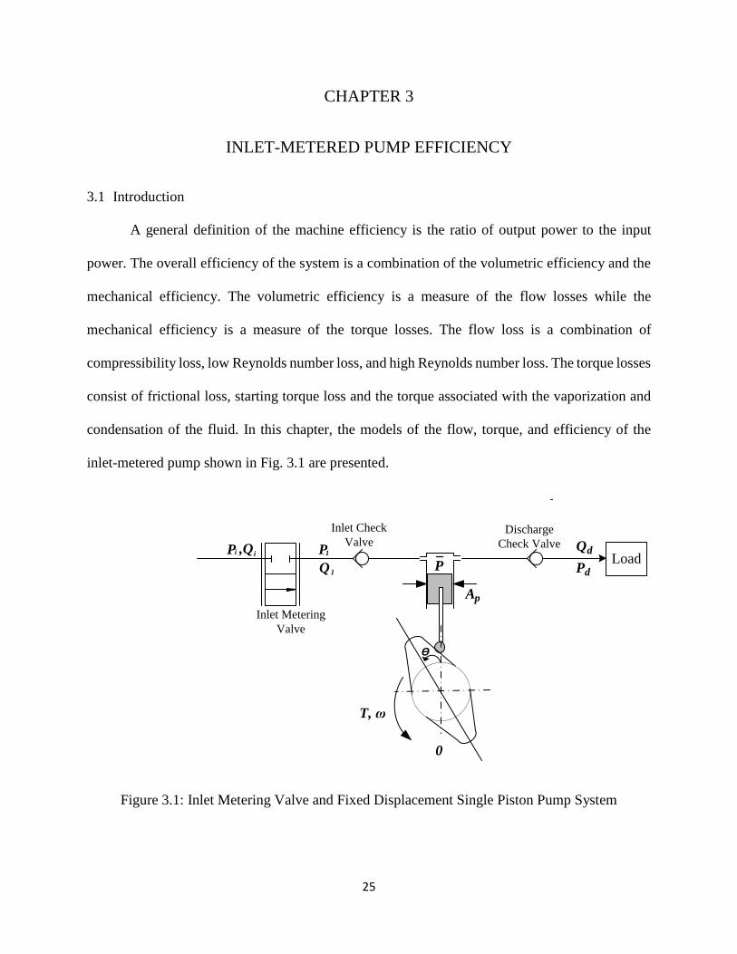
condensation of the fluid. In this chapter, the models of the flow, torque, and efficiency of the
inlet-metered pump shown in Fig. 3.1 are presented.
iP ,Qi
T, ω
Pd
Qd
Ap
P
1
1
P
0
Ѳ
Inlet Check
ValveDischarge
Check Valve
Q
Inlet Metering
Valve
Load
Figure 3.1: Inlet Metering Valve and Fixed Displacement Single Piston Pump System
Page 43
26
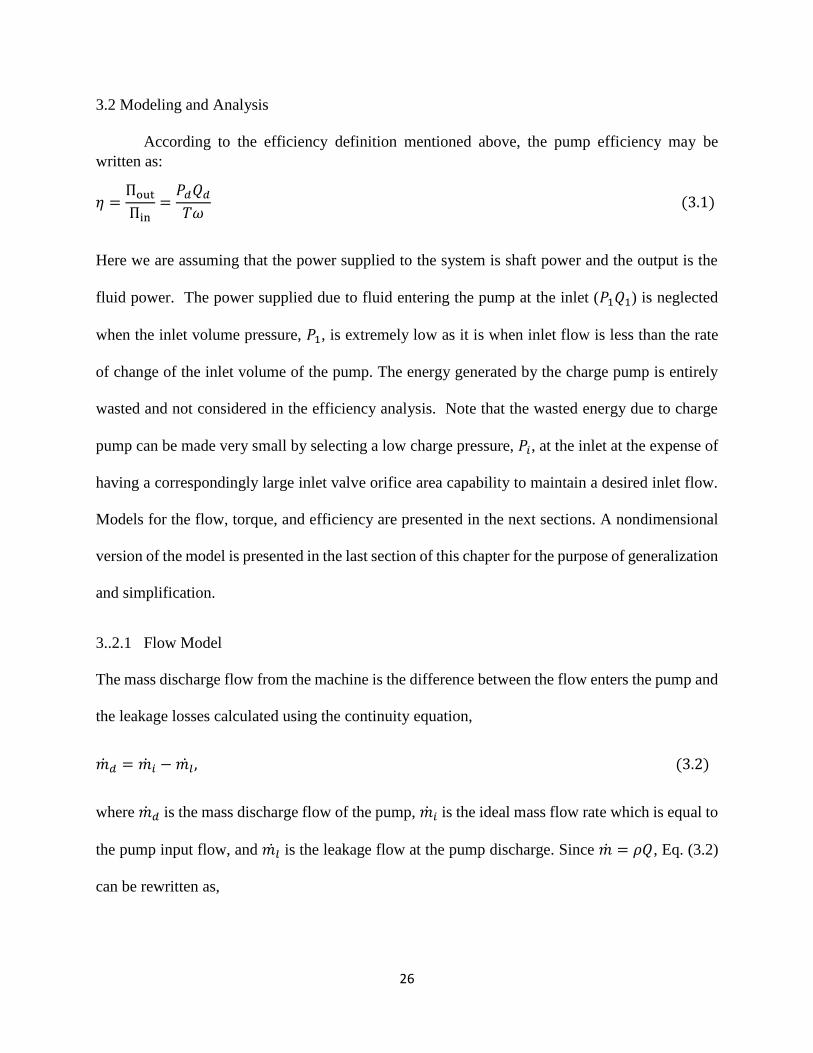
3.2 Modeling and Analysis
According to the efficiency definition mentioned above, the pump efficiency may be
written as:
𝜂 =ПoutПin
=𝑃𝑑𝑄𝑑𝑇𝜔
(3.1)
Here we are assuming that the power supplied to the system is shaft power and the output is the
fluid power. The power supplied due to fluid entering the pump at the inlet (𝑃1𝑄1) is neglected
when the inlet volume pressure, 𝑃1, is extremely low as it is when inlet flow is less than the rate
of change of the inlet volume of the pump. The energy generated by the charge pump is entirely
wasted and not considered in the efficiency analysis. Note that the wasted energy due to charge
pump can be made very small by selecting a low charge pressure, 𝑃𝑖, at the inlet at the expense of
having a correspondingly large inlet valve orifice area capability to maintain a desired inlet flow.
Models for the flow, torque, and efficiency are presented in the next sections. A nondimensional
version of the model is presented in the last section of this chapter for the purpose of generalization
and simplification.
3..2.1 Flow Model
The mass discharge flow from the machine is the difference between the flow enters the pump and
the leakage losses calculated using the continuity equation,
��𝑑 = ��𝑖 −𝑚𝑙 , (3.2)
where ��𝑑 is the mass discharge flow of the pump, ��𝑖 is the ideal mass flow rate which is equal to
the pump input flow, and 𝑚𝑙 is the leakage flow at the pump discharge. Since �� = 𝜌𝑄, Eq. (3.2)
can be rewritten as,
Page 44
27
𝑄𝑑 =𝜌𝑖𝜌𝑑(𝑄𝑖) − 𝑄𝑙. (3.3)
The density ratio may be determined from the following equation [33],
𝜌 = 𝜌oExp (𝑃
𝛽), (3.4)
where 𝜌o is the density at zero pressure and β is the fluid bulk modulus which was assumed to be
constant. Note that in Eq. (3.4), the symbol, P, is used for pressure in general -- this equation would
not apply to the pressure, P, inside the cylinder due to the prevalence of undissolved gases (air).
Then, the ratio of the fluid density at the pump inlet, 𝜌𝑖, and the fluid desity at the pump discharge,
𝜌𝑑, is defined as follows for the inlet and discharge pressure volumes:
𝜌𝑖𝜌𝑑
= Exp (𝑃𝑑𝛽) ≈ 1 −
𝑃𝑑𝛽= 1 − 𝑘0𝑃𝑑 , (3.5)
where 𝜌i and 𝜌d are the fluid densities at the inlet and the discharge respectively and k0 accounts
for the effect of fluid compressibility. The ideal volumetric flow rate, 𝑄𝑖, associated with the fixed
displacement pump with an inlet metering valve will be modeled using the orifice equation,
𝑄𝑖 = 𝐴𝑣𝐶𝑑√2(𝑃𝑖 − 𝑃1)
𝜌 (3.6)
where 𝑃𝑖 is pressure of the charge pump, P1 is the pressure at the exit of the inlet metering valve
which has been assumed to be approximately zero, 𝐴𝑣 is the valve metering area, and 𝐶𝑑 is the
discharge coefficient. Equation (3.6) is valid as long as the ideal discharge flow does not exceed
the maximum flow for a given pump speed i.e. the flow is not restricted by the product pump speed
and displacement volume and it is a function of only the valve opening. This means that the valve
area has a maximum value such that,
Page 45
28
𝐴𝑣 ≤𝑉𝑑𝜔
𝐶𝑑√2𝑃𝑖𝜌
. (3.7)
Once the valve opening area exceeds the condition in Eq. (3.7), the ideal flow is simply the product
of the volumetric displacement and the pump speed. The internal leakage flow loss is modeled as
a combination of high and low Reynolds number flows and is given by
𝑄𝑙 = 𝑘11
𝜇𝑃𝑑 + 𝑘2√𝑃𝑑 . (3.8)
where 𝑘1 and 𝑘2 are the low Reynolds and the high Reynolds number leakage coefficients,
respectively. Substitution of Eq. (3.5) into Eq. (3.4), substituting that result along with Eq. (3.6)
into Eq. (3.8) gives the discharge flow,
𝑄𝑑 = (1 − 𝑘0𝑃𝑑)𝐴𝑣𝐶𝑑√2𝑃𝑖𝜌−𝑘1
1
𝜇𝑃𝑑 − 𝑘2√𝑃𝑑 . (3.9)
Three key coefficients are used in the description of volumetric flow rate: fluid compression, K0,
the low Reynolds number leakage, K1, and the high Reynolds number leakage, K1. Notice that the
flow is only a function of valve opening area if losses are neglected. Note that there is a limitation
on the inlet flow and therefore discharge flow cannot exceed the product of the volumetric
displacement and pump shaft speed.
The valve opening area, Av, is given in (3.10) and was obtained from flow versus voltage data
due to an experiment where the discharge pressure was very low with the inlet pressure held
constant. The computed valve area is plotted versus voltage and compared to a curve fit in Fig. 4.
The quadratic polynomial that relates the valve opening area (m2) to the voltage, V, is shown in
Eq. (3.10):
Page 46
29
𝐴𝑣 = 0.97 × 10⁻⁷𝑉2 + 2.29 × 10⁻⁶𝑉 − 0.54 × 10⁻⁶ (3.10)
3.2.2 Torque Model
The torque required by the inlet metering pump is a combination of four components; ideal
torque, 𝑇𝑖𝑑𝑒𝑎𝑙, torque required to force the trapped air out and to condense the fluid vapor, 𝑇𝑐,
friction torque, 𝑇𝑓, and the starting torque, 𝑇𝑠, which includes the constant torque resulting from
the spring that holds the piston down. Then, the total torque can be written as:
𝑇 = 𝑇𝑖𝑑𝑒𝑎𝑙 + 𝑇𝑐 + 𝑇𝑓 + 𝑇𝑠 (3.11)
The ideal torque may be written as the output power divided by the pump speed,
𝑇𝑖𝑑𝑒𝑎𝑙 =𝑃𝑑𝑄𝑑𝜔
=𝑃𝑑𝐴𝑣𝐶𝑑√
2𝑃𝑖𝜌
𝜔 (3.12)
The torque required to compress the partially vaporized fluid and to force air out of or into the
fluid solution was found to have a linear relationship with the difference between the pump
maximum and actual flows [74] and can be written as 𝑇𝑐 = 𝜓(𝑄𝑚𝑎𝑥 − 𝑄𝑑) where 𝜓 is a constant
and its value depends on the working fluid. If Eq. (3.6) is used as an approximation for the
discharge flow, the compression torque becomes,
𝑇𝑐 = 𝜓(𝑉𝑑𝜔 − 𝐴𝑣𝐶𝑑√2𝑃𝑖𝜌) (3.13)
The friction torque is [33]
𝑇f = 𝑇ideal. 𝜇s (3.14)
where µs is the coefficient of friction existing within the machine. The coefficient of friction is
modeled by Stribeck curve (Fig.2) as follows:
Page 47
30
𝜇s = 𝐴′Exp (−𝐵′𝜇𝑈
𝑊) + 𝐶′√
𝜇𝑈
𝑊 (3.15)
Where 𝐴′, 𝐵′, and 𝐶′ are constants, 𝜇 is the fluid viscosity, U is the sliding velocity, and W is the
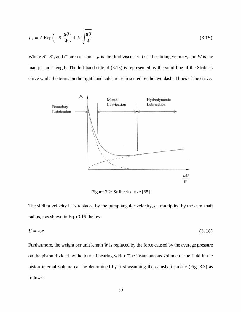
load per unit length. The left hand side of (3.15) is represented by the solid line of the Stribeck
curve while the terms on the right hand side are represented by the two dashed lines of the curve.
Figure 3.2: Stribeck curve [35]
The sliding velocity U is replaced by the pump angular velocity, ω, multiplied by the cam shaft
radius, r as shown in Eq. (3.16) below:
𝑈 = 𝜔𝑟 (3. 16)
Furthermore, the weight per unit length W is replaced by the force caused by the average pressure
on the piston divided by the journal bearing width. The instantaneous volume of the fluid in the
piston internal volume can be determined by first assuming the camshaft profile (Fig. 3.3) as
follows:
Page 48
31
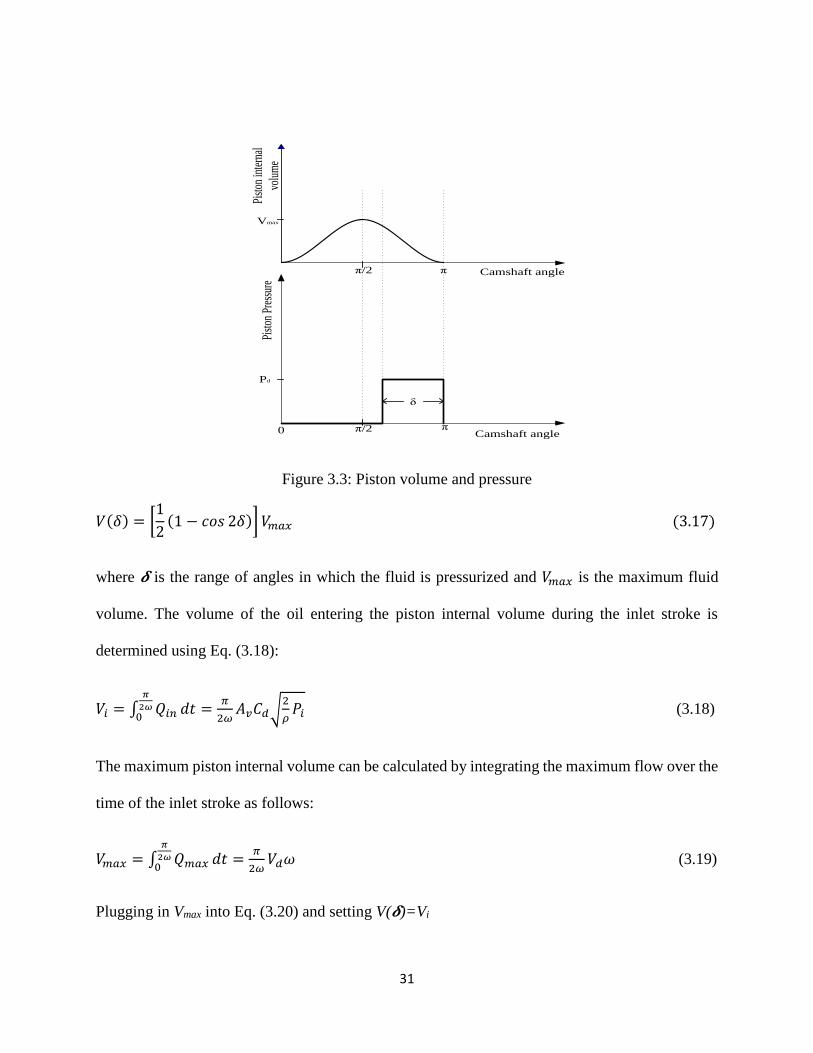
Figure 3.3: Piston volume and pressure
𝑉(𝛿) = [1
2(1 − 𝑐𝑜𝑠 2𝛿)] 𝑉𝑚𝑎𝑥 (3.17)
where 𝜹 is the range of angles in which the fluid is pressurized and 𝑉𝑚𝑎𝑥 is the maximum fluid
volume. The volume of the oil entering the piston internal volume during the inlet stroke is
determined using Eq. (3.18):
𝑉𝑖 = ∫ 𝑄𝑖𝑛𝜋
2𝜔0
𝑑𝑡 =𝜋
2𝜔𝐴𝑣𝐶𝑑√
2
𝜌𝑃𝑖 (3.18)
The maximum piston internal volume can be calculated by integrating the maximum flow over the
time of the inlet stroke as follows:
𝑉𝑚𝑎𝑥 = ∫ 𝑄𝑚𝑎𝑥𝜋
2𝜔0
𝑑𝑡 =𝜋
2𝜔𝑉𝑑𝜔 (3.19)
Plugging in Vmax into Eq. (3.20) and setting V(𝜹)=Vi
δ
Pist
on P
ress
ure
Pd
π/20 πCamshaft angle
Pist
on in
tern
al
volu
me
π/2 π Camshaft angle
Vmax
Page 49
32
𝛿 =1
2cos−1
(
1 −2𝐴𝑣𝐶𝑑√
2𝜌 𝑃𝑖
𝜔𝑉𝑑)
(3.20)
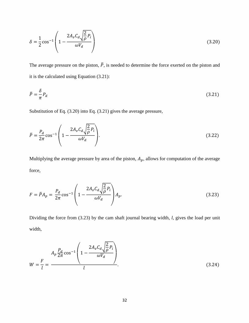
The average pressure on the piston, ��, is needed to determine the force exerted on the piston and
it is the calculated using Equation (3.21):
�� =𝛿
𝜋𝑃𝑑 (3.21)
Substitution of Eq. (3.20) into Eq. (3.21) gives the average pressure,
�� =𝑃𝑑2𝜋
cos−1
(
1 −2𝐴𝑣𝐶𝑑√
2𝜌 𝑃𝑖
𝜔𝑉𝑑)
. (3.22)
Multiplying the average pressure by area of the piston, 𝐴𝑝, allows for computation of the average
force,
𝐹 = ��𝐴𝑝 = 𝑃𝑑2𝜋
cos−1
(
1 −2𝐴𝑣𝐶𝑑√
2𝜌𝑃𝑖
𝜔𝑉𝑑)
𝐴𝑝. (3.23)
Dividing the force from (3.23) by the cam shaft journal bearing width, l, gives the load per unit
width,
𝑊 =𝐹
𝑙=
𝐴𝑝𝑃𝑑2𝜋 cos
−1
(
1 −2𝐴𝑣𝐶𝑑√
2𝜌𝑃𝑖
𝜔𝑉𝑑)
𝑙. (3.24)
Page 50
33
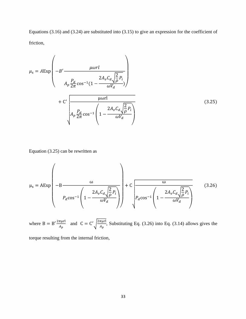
Equations (3.16) and (3.24) are substituted into (3.15) to give an expression for the coefficient of
friction,
𝜇s = 𝐴Exp
(
−𝐵′𝜇𝜔𝑟𝑙
𝐴𝑝𝑃𝑑2𝜋 cos
−1(1 −2𝐴𝑣𝐶𝑑√
2𝜌 𝑃𝑖
𝜔𝑉𝑑))
+ C′
√ μωrl
𝐴𝑝𝑃𝑑2𝜋 cos
−1
(
1 −2𝐴𝑣𝐶𝑑√
2𝜌 𝑃𝑖
𝜔𝑉𝑑)
(3.25)
Equation (3.25) can be rewritten as
μs = AExp
(
−Bω
𝑃𝑑cos−1
(
1 −2𝐴𝑣𝐶𝑑√
2𝜌 𝑃𝑖
𝜔𝑉𝑑)
)
+ C
√ ω
𝑃𝑑cos−1
(
1 −2𝐴𝑣𝐶𝑑√
2𝜌𝑃𝑖
𝜔𝑉𝑑)
(3.26)
where B = B′2𝜋μrl
𝐴𝑝 and C = C′√
2𝜋μrl
𝐴𝑝, Substituting Eq. (3.26) into Eq. (3.14) allows gives the
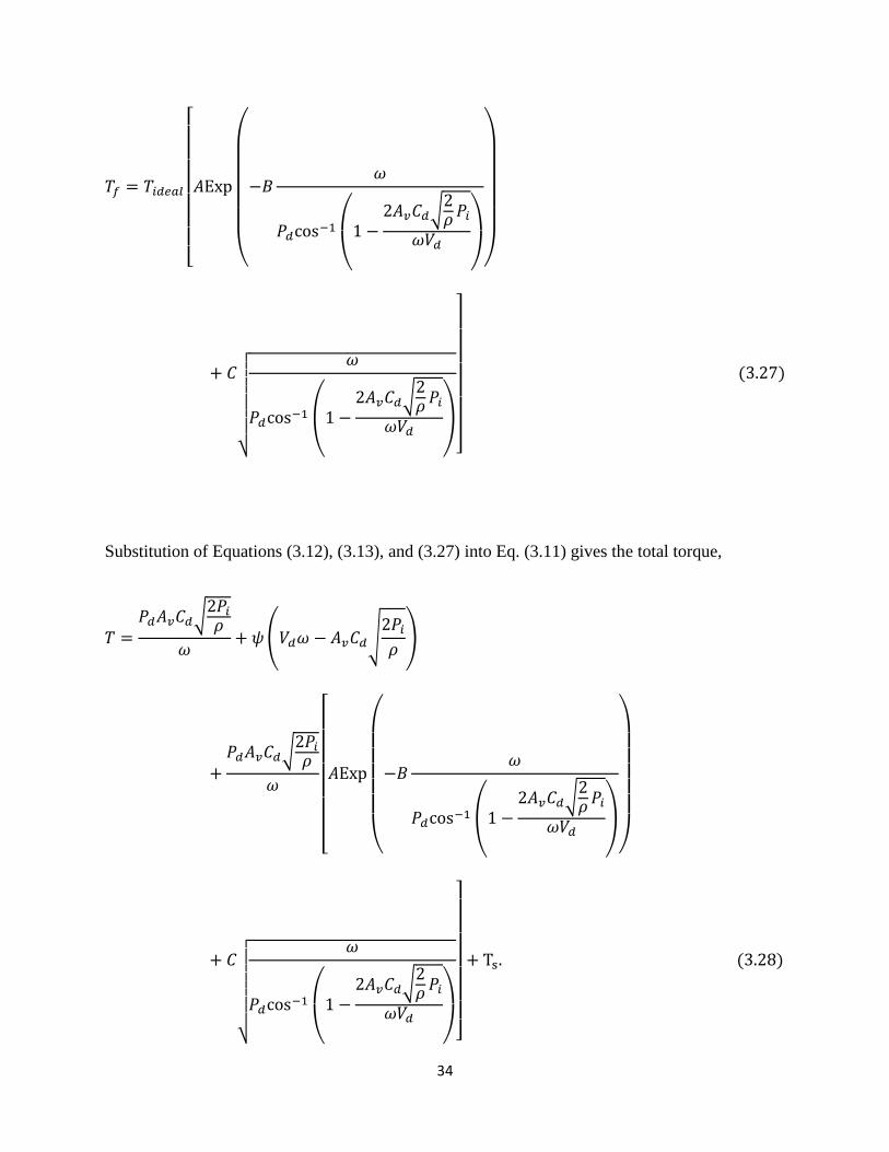
torque resulting from the internal friction,
Page 51
34
𝑇𝑓 = 𝑇𝑖𝑑𝑒𝑎𝑙
[
𝐴Exp
(
−𝐵𝜔
𝑃𝑑cos−1
(
1 −2𝐴𝑣𝐶𝑑√
2𝜌𝑃𝑖
𝜔𝑉𝑑)
)
+ 𝐶
√ 𝜔
𝑃𝑑cos−1
(
1 −2𝐴𝑣𝐶𝑑√
2𝜌 𝑃𝑖
𝜔𝑉𝑑)
]
(3.27)
Substitution of Equations (3.12), (3.13), and (3.27) into Eq. (3.11) gives the total torque,
𝑇 =𝑃𝑑𝐴𝑣𝐶𝑑√
2𝑃𝑖𝜌
𝜔+ 𝜓(𝑉𝑑𝜔 − 𝐴𝑣𝐶𝑑√
2𝑃𝑖𝜌)
+𝑃𝑑𝐴𝑣𝐶𝑑√
2𝑃𝑖𝜌
𝜔
[
𝐴Exp
(
−𝐵𝜔
𝑃𝑑cos−1
(
1 −2𝐴𝑣𝐶𝑑√
2𝜌𝑃𝑖
𝜔𝑉𝑑)
)
+ 𝐶
√ 𝜔
𝑃𝑑cos−1
(
1 −2𝐴𝑣𝐶𝑑√
2𝜌 𝑃𝑖
𝜔𝑉𝑑)
]
+ Ts. (3.28)
Page 52
35
3.2.3 Model Nondimensionalization
To generalize the model, the equation parameters are normalized about selected reference
conditions. Nondimensionalizing the equation also gives a simpler form of the equations with
reduced number of parameters. The following definitions were used to nondimensionalize the
equations:
𝜔 = ��𝜔𝑟,
𝑄𝑑 = ��𝑑𝑉𝑑𝜔𝑟,
𝑃𝑑 = ��𝑑𝑃𝑑𝑟,
𝑃𝑖 = ��𝑖𝑃𝑖𝑟,
𝐴𝑣 = ��𝑣𝑉𝑑𝜔𝑟
𝐶𝑑√2𝑃𝑖𝑟𝜌
,
and
𝑇 = ��𝑃𝑑𝑟𝑉𝑑.
The subscript (r) refers to the reference condition that was chosen such that, Pdr=25 MPa, ωr=2500
RPM, and, Pir=2 MPa. The volumetric displacement is Vd=1.3375×10⁻⁶ m3 per radian of the pump
shaft rotation Applying the above definitions, the flow in Eq. (3.9) can be written in a
nondimensional form as:
��𝑑 = ��𝑣√��𝑖 − ��0��𝑣��𝑑√��𝑖 − ��1��𝑑 − ��2√��𝑑 (3.29)
where
��0 = 𝑘0𝑃𝑑𝑟𝐴𝑟√𝑃𝑖𝑟,
Page 53
36
��1 = 𝑘1𝑃𝑑𝑟
𝜇𝑉𝑑𝜔𝑟, and
��2 = 𝑘2√𝑃𝑑𝑟
𝑉𝑑𝜔𝑟.
Similarly, the torque equation (3.28) is written in nondimensional form as
�� =��𝑑��𝑣√��𝑖
��+ �� (�� − ��𝑣√��𝑖)
+��𝑑��𝑣√��𝑖
��
[
��𝐸𝑥𝑝
(
−��
��
��𝑑 cos−1 (1 −2��𝑣√��𝑖��
))
+ ��√
��
��𝑑 cos−1 (1 −2��𝑣√��𝑖��
)]
+ ��𝑠, (3.30)
where �� = 𝜓𝜔𝑟
𝑃𝑑𝑟, �� = 𝐴, �� = 𝐵
𝜔𝑟
𝑃𝑑𝑟, �� = 𝐶√
𝜔𝑟
𝑃𝑑𝑟, and, ��𝑠 =
𝑇𝑠
𝑃𝑑𝑟𝑉𝑑.
The coefficients ��, ��, ��, ��, and ��𝑠 are determined from experiments. Equation (3.30) may be
rewritten as:
�� =��𝑑��𝑣√��𝑖
��+ �� (�� − ��𝑣√��𝑖) +
��𝑑��𝑣√��𝑖��
[��𝑋 + ��𝑌] + ��𝑠 , (3.31)
where
𝑋 = 𝐸𝑥𝑝
(
−��
��
��𝑑 cos−1 (1 −2��𝑣√��𝑖��
))
Page 54
37
and
𝑌 =√
��
��𝑑 cos−1 (1 −2��𝑣√��𝑖��
)
Equation (3.1) can then be nondimensionalized to give a nondimensional expression for the pump overall
efficiency,
η =𝑃𝑑𝑄𝑑𝑇𝜔
=��𝑑��𝑑
����. (3.32)
Page 55
38
CHAPTER 4
EXPERIMENTAL SETUP
4.1 Introduction
This chapter aimed at presenting the details of the experimental setup. The description of
the inlet-metering system prototype used in this work is presented in this chapter. Details of the
study-state and transient tests that are performed in this study are also presented. In addition,
photos of the inlet-metering system prototype components with their details are also found in this
chapter.
4.2 Test Setup
The IMP was tested using the hydraulic circuit given in Fig. 4.1 with Caterpillar Hydo
Advanced 10 oil. In the circuit, there are several flow, pressure, and temperature sensors. A
pressure-controlled pump generates the inlet flow. The discharge flow of the inlet-metered pump,
IMP, travels through parallel paths with a flow control valve or a relief valve. After the valves,
the flow is returned to the reservoir. More details are given in Fig. 4.1 such as sensor locations.
The descriptions of the sensors are given in Table 4.1. The IMP is driven by a variable speed drive
(a synchronous AC motor controlled by a variable frequency voltage source). Test speeds ranged
from ~3 rpm up to 2500 rpm. Most tests were conducted with the relief valve and supply pressures
set at constant values with the flow control valve closed. The inlet-metering valve, IMV, (flow
control inside the dashed box in Fig. 4.1) was controlled by a modified Caterpillar engine
controller. The controller was modified by Caterpillar engineers so that the IMV position
command could be manipulated by an external voltage signal. This voltage signal was generated
by a PC based data acquisition system.
Page 56
39
The data acquisition was accomplished using a PC with data acquisition expansion card.
The expansion card has a 32 channel 16-bit analog input and 4 channel counter timer capabilities.
The analog inputs were used to obtain valve feedback, pressure, and temperature signals while the
counter timers were used to interpret the digital flow meter signals. The system also has analog
output capabilities which were used to generate voltage signals sent to the Caterpillar engine
controller to manipulate the IMV opening. Serial (RS-232) communication was used to obtain
torque measurements. Speed signals were not acquired using the computer but instead read from
a digital readout. Speed signals were found to not vary significantly due to the speed regulation
capabilities of the motor drive system. The drive has very high inertia and extremely steep torque
rise with decreasing speed.
There were additional measurements utilized in some tests. The acceleration of the pump
housing was measured using a Caterpillar knock sensor (P/N 195-2431). The pump head
temperature was also measured using a temperature sensor built into the fuel pump head manifold.
Page 57
40
Flow Meter
Discharge
Flow
Control
Valve
Pressure
Control
Safety
Relief
Relief
M
VFD
AC Motor
Inlet
Metering
PumpTorque,
Speed
Sensor
Pd
Pi
Tempd
Tempi
M
Fixed
AC
Motor
Flow
Control
Oil Cooler
Heat
Exchanger
Unloading Valve
Flow Meter
Inlet.
Drain
Figure 4.1. Inlet metering pump testing circuit diagram
Page 58
41
Table 4.1 Measurements
Symbol Description Identifying Information
Pd Discharge Pressure BT91760CC-102-15-002 (Setra)
Pi Inlet Pressure UB020867 40 (Setra)
Qi Inlet Flow KY18435224 (Gear type)
Qd Discharge Flow KY18438224 (Gear type)
T Applied Torque 48202V(1-3) (Himmelstein +/-1000 in-lb)
𝜔 Motor Speed Same as torque
V Inlet Valve Voltage NI DAQ card
Th Head Temperature Sensor integrated into pump
Ti Inlet Temperature Same as inlet pressure
Td Discharge Temperature Same as discharge pressure
The experimental setup is shown in Fig. 4.2. The installed pump is shown in Fig.4.3.
Various hoses and manifolds were used to complete the hydraulic circuit setup. In Fig. 4.3, the
pump is seen attached to a tube with an adapter that contains the torque sensor. This tube is bolted
to the 200 hp electric motor. The lubrication line can be seen connecting to the pump housing near
the point where the housing meets the adapter. This lubrication line is connected to the charge
pump through a pressure reducing valve set at 50 psi (344 kPa). The lubrication system primarily
supplies fluid flow to the journal bearings that supports the motor driven cam that drives the piston
displacement. The flow from these journal bearings leaks into the pump case and then directly into
the adapter tube containing the torque sensor. This flow is carried away by a small impeller pump
and returned to the reservoir. This is a nonconventional setup that allows for testing of the pump
Page 59
42
which was originally designed to receive lubrication pressure from an engine lubrication system.
The engine lubricant was designed to flow back into the engine crankcase where the pump would
normally be attached.
Figure 4.2. Inlet metering system experimental setup
Page 60
43
Figure 4.3. Installed pump connected to the torque sensor housing and hydraulic hoses.
4.3 Steady State Testing
For steady state tests, inlet pressure, discharge pressure, IMV voltage, and pump speeds
were set in combinations for 10-second periods. Pump speeds were set to 200, 500, 1000, 1500,
and 2500 rpm. The inlet pressure was set to 2, 2.5, 3, and 3.5 MPa. The discharge pressure was set
to 2, 5, 10, 20, and 25 MPa. Note that the pressure settings were made while the pump was
operating with the maximum IMV valve command and varied when the pump flow varied with
the valve command. The valve voltage command was set to 0, 0.5, 1, 2, 3, 4, and 5 volts.
For each test, pressure and speed settings were made – and a MATLAB SIMULINK®
program was used to vary the voltage in steps from zero to 5 volts holding at each level for 10
seconds. Note that the steady state testing data also includes some transient information due to the
step changes in IMV voltage. After the tests were completed, the average values for each 10 second
period were computed and stored for later analysis. In total, there were over 600 different test
conditions obtained. Table 4.2 summarizes the steady-state test conditions.
Page 61
44
Table 4.2. Data collection points associated with experiments.
Pump inlet pressure [MPa] Pump discharge pressure [MPa] Pump shaft speed [RPM]
2.0 2.0, 5.0, 10.0, 20.0, 25.0 200, 500, 1000, 1500, 2500
2.5 2.0, 5.0, 10.0, 20.0, 25.0 200, 500, 1000, 1500
3.0 2.0, 5.0, 10.0, 20.0, 25.0 200, 500, 1000, 1500
3.5 2.0, 5.0, 10.0, 20.0, 25.0 200, 500, 1000, 1500
4.4 Transient Testing
Transient testing was completed using dynamic signals for the IMV voltage command.
These signals include modulation, step, and chirp signals. Pressure and speed settings were held
constant. Quasi-steady tests in the form of voltage modulations were also completed. The IMV
voltage was modulated from zero to 5 volts while holding speed and pressures constant. Chirp
signals were supplied to the IMV valve command to validate the model for different dynamic
conditions. The frequency range included 0.1 to 30 Hz. Additional step responses were measured
while the flow control valve was opened. This allowed for a dynamic response in the pressure
signal when flow varied due to a step change in the IMV valve command.
4.5 Inlet-metering valve and Pump Components
The photos of the pump components are given in the following figures with their
description. Both inlet and discharge poppet valves have springs that hold them closed in addition
to pressure forces. The spring on the inlet poppet is captured within a screw in housing. The inlet
poppet spring was found to be especially stiff and was held open for the photograph (the stiffness
was not measured). The IMV is a rotary actuated valve driven by a servomotor (motor is not
Page 62
45
shown). In the photos, it can be seen that there is no damage visible on any components. There is
damage on the journal bearing inserts, possibly due to initial startup or poor lubrication. Poor
lubrication could be due to using hydraulic oil for lubrication rather than engine oil that is present
when the pump is used in engine fuel pumping applications. In addition, it was noted that there
was an extremely large amount of air in the lubrication oil flow exiting the pump crank case. The
air in the fluid would have degraded the lubrication in the journal bearing.
Figure 4.4. Piston side view (length of largest diameter is 59 mm, overall length is 103 mm)
Page 63
46
Figure 4.5. Piston crown
Figure 4.6. Pump cylinder
Page 64
47
Figure 4.7. Cylinder head with inlet check on the side and discharge check valve placed on top.
The discharge poppet (Fig. 4.7) is designed to have damped motion to help slow closing
speeds in the fuel pump application. It is believed that this damped design contributes to flow
moving back into the pump cylinder during the intake phase of the pump operation. This is
believed to reduce the volumetric efficiency significantly. Redesigning the discharge check valve
would likely improve the volumetric efficiency of the pump. Much less damping is needed in the
discharge check valve for a hydraulic system due to the dramatically lower pressures at the pump
discharge. For example, in a hydraulic system pressures of around 30 MPa are needed compared
to 300 MPa in the fuel pump application. Due to the lower pressures in a hydraulic system, much
less damping could be utilized to reduce volumetric losses while still protecting the valve from
damage due to rapid closing.
Page 65
48
Figure 4.8. Inlet poppet (held open).
Figure 4.9. Discharge poppet.
Page 66
49
Figure 4.10. Discharge poppet seat.
Figure 4.11. Cam lobe.
Page 67
50
Figure 4.12. Journal bearing insert in the pump housing end cap.
Page 68
51
Figure 4.13. IMV sub assembly. The round part of the keyhole shape has a diameter of 7.5 mm.
The flat part of the keyhole shape has a diameter of 5mm. The inner part of the valve rotates
changing the size of the triangular flow area.
Page 69
52
Figure 4.14. IMV disassembled. The dimensions of the triangle portion in the valve are
approximately 2.7 mm x 8 mm.
Figure 4.15. Case drain for lubrication flow, highly aerated.
Page 70
53
CHAPTER 5
VELOCITY CONTROL SYSTEM DESIGN
5.1 Introduction
Hydraulic linear actuators are used to convert the pressurized fluid energy into mechanical
energy that is used to move loads linearly. Hydraulic actuators are used in many motion control
applications such as in off-highway machinery, aircraft, automotive, and industrial machinery. The
velocity of hydraulic actuators is controlled by manipulating the flow entering the actuator. This
chapter presents a theoretical model and methods for designing a velocity control system for a
hydraulic actuator using an inlet metering pump system to control the fluid flow to a hydraulic
cylinder. The velocity control system for a linear actuator is shown in Figure 1. The system consists
of an inlet metering pump system, a four-way directional valve, and a linear actuator. The four-
way valve is a wide open switching valve and it is used to switch the flow direction to one of the
actuator ports depending on the desired direction of the hydraulic cylinder. The discharge flow is
supplied to one of the actuator ports, as required, using a four-way directional valve. The flow
from the other port of the actuator is returned to the tank through the four-way directional valve.
Page 71
54
4-way
directional
valve
Inlet Metering System
iP ,Q i
Charge
Pump
Relief Valve
T, ω
Pd
Qd
Ap
P
1
1
P
0
Ѳ
Inlet Check
ValveDischarge
Check Valve
Q
Inlet
Metering
Valve
x
m
PA
PB
QA
QB
FK
u
AA
y, v
b
Figure 5.1: Velocity Control System for a Linear Actuator
5.2 Modeling the system
The following assumptions are made for creating a model for the system. Let 𝑃𝐴 =
𝑃𝑑, assuming that the size of directional valve orifice is large enough so that there is no
restriction on the flow through the valve which means that the pressure drop through the
passages and directional control valve are small. The system is modeled as if there is one
volume extending from the discharge check valve to the piston surface. Since this is a piston
pump, flow from a single piston would be discontinuous. However, we assume that multiple
pistons would be used and therefore only consider the average flow and do not model any
flow ripple or discontinuity (to be considered in future work). The governing equations
include the equation of motion of the linear actuator and the pressure rise rate equation. The
equation of motion can be written as:
𝑚�� + 𝑏�� + 𝑘𝑦 −𝑚𝑔 = 𝜂𝑎𝑓𝑃𝑑𝐴𝐴 − 𝐹𝑜 − 𝐹 (5.1)
For steady state conditions, = �� = �� = 0 , 𝐹 = 0 and 𝑃𝑑 = 0, then, 𝐹𝑜 = 𝑚𝑔. In this
analysis, we will consider 𝐹𝑜 = 𝑚𝑔 for all cases. Also, the load spring is usually not included
Page 72
55
in analysis where the goal of which is controlling the velocity [75], i.e., k=0. So, the equation
of motion becomes,
𝑚�� + 𝑏𝑣 = 𝜂𝑎𝑃𝑑𝐴𝐴 − 𝐹 (5.2)
where the cylinder velocity, 𝑣 = ��. The pressure rise rate equation is written as:
��𝑑 =𝛽
𝑉𝑜 + 𝐴𝐴𝑦(𝑄𝑖 − 𝑘1𝑃𝑑 − 𝐴𝐴𝑣) (5.3)
where 𝑄𝑖 is the inlet flow which is equal to the ideal discharge flow of the inlet-metered
pump and defined in Eq. (5.4).
𝑄𝑖 = 𝐶𝑑𝐴𝑣√2𝑃𝑖𝜌 (5.4)
The relationship between valve area and flow through the inlet metering pump given
in Eq. (5.4) was derived in Chapter 3. The leakage coefficient, 𝑘1 was assumed to have a
constant value and to account for leakage in the cylinder and other flow losses such as in the
pump. A reasonable value for the leakage coefficient is 𝑘1 =𝑄𝑚𝑎𝑥
10𝑃𝑚𝑎𝑥.
Equation (5.3) may be linearized using the following nominal conditions: 𝑦𝑜 = 𝑣 =
𝑄𝑑𝑜 = 𝑃𝑑𝑜 = 0. The linearized equation for the pressure rise rate is,
��𝑑 =𝛽
𝑉𝑜(𝑄𝑖 − 𝑘1𝑃𝑑 − 𝐴𝐴𝑣) (5.5)
Substituting Eq. (5.4) into Eq. (5.5) gives:
��𝑑 =𝛽
𝑉𝑜(𝐶𝑑𝐴𝑣√
2𝑃𝑖𝜌− 𝑘1𝑃𝑑 − 𝐴𝐴𝑣) (5.6)
Page 73
56
In order to generalize the model, all the quantities in Eqs. (5.2) and (5.6) are normalized
about reference conditions. Eq. (5.2) can be nondimensionalized using the following
reference conditions:
𝑃𝑑 = ��𝑑𝑃𝑑𝑟, 𝑣 = 𝑣𝑣𝑟 𝐴𝑣 = ��𝑣𝐴𝑟 , 𝑃𝑖 = ��𝑖𝑃𝑖𝑟 and 𝑡 = ��𝜏.
Using these reference conditions, Eq. (5.6) can be written as:
𝑑(��𝑑𝑃𝑑𝑟)
𝑑(��𝜏)=𝛽
𝑉𝑜(𝐶𝑑𝐴𝑟√
2𝑃𝑖𝑟𝜌
��𝑣√��𝑖 − 𝑘1��𝑑𝑃𝑑𝑟 − 𝐴𝐴𝑣𝑟𝑣) (5.7)
Multiplying Eq. (5.7) by 𝜏/𝑃𝑑𝑟 gives:
��𝑑 =𝜏𝛽
𝑉𝑜𝑃𝑑𝑟𝐶𝑑𝐴𝑟√
2𝑃𝑖𝑟𝜌
��𝑣√��𝑖 −𝜏𝛽
𝑉𝑜𝑘1��𝑑 −
𝜏𝛽𝑣𝑟𝑉𝑜𝑃𝑑𝑟
𝐴𝐴𝑣 (5.8)
Let
𝜏 =𝑉𝑜𝛽𝑘1
then, that the nondimensional pressure rise equation can be written as:
��𝑑 + ��𝑑 = 𝜉1��𝑣√��𝑖 − 𝜉2v (5.9)
where the nondimensional groups 𝜉1 and 𝜉2 in Eq. (5.9) are defined as
𝜉1 =𝐶𝑑𝐴𝑟√
2𝑃𝑖𝑟𝜌
𝑃𝑑𝑟𝑘1, and
𝜉2 =𝜏𝛽𝑣𝑟𝐴𝐴𝑉𝑜𝑃𝑑𝑟
.
Page 74
57
Similarly, using the reference conditions mentioned above, Eq. (5.2) may be written in
nondimensional form as:
𝑚𝑑(𝑣𝑣𝑟)
𝑑(��𝜏)+ 𝑏𝑣𝑣𝑟 = 𝜂𝑎𝑓𝑃𝑑𝐴𝐴 − 𝐹 (5.10)
Dividing Eq. (5.10) by 𝑃𝑑𝑟𝐴𝐴 gives:
���� + ��𝑣 = 𝜂𝑎𝑓��𝑑 − �� (5.11)
where
{
�� =
𝑚𝑣𝑟𝑃𝑑𝑟𝐴𝐴𝜏
�� =𝑏𝑣𝑟𝑃𝑑𝑟𝐴𝐴
��𝐴 =𝐴𝐴𝐴𝐴
= 1
�� =𝐹
𝑃𝑑𝑟𝐴𝐴 }
(5.12)
5.3 Stability Analysis
From Eqs. (5.9) and (5.11) the dynamic system equations can be written in state-space
matrix form, i.e.,
�� = 𝐴𝒙 + 𝐵𝒖 and 𝑦 = 𝐶𝒙 + 𝐷𝒖.
Let 𝒙 = [��𝑑 𝑣]𝑇, 𝒖 = [��𝑣 ��]
𝑇 and 𝒚 = 𝑣. By examining Eqs. (5.9) and (5.11), the
matrices A, B, C, and D can be found to be,
𝐴 = [
−1 −𝜉2𝜂𝑎��
−��
��
],
Page 75
58
𝐵 =
[ 𝜉1√��𝑖 0
0 −1
��] ,
𝐶 = [0 1], and
𝐷 = 0.
For stability analysis, the characteristic equation can be computed,
det(𝑠𝐼 − 𝐴) = 𝑠2 + (��
��+ 1) 𝑠 + (
�� + 𝜂𝑎𝜉2��
) = 0
The coefficients in the characteristic equation are:
{
𝑎𝑜 = 1
𝑎1 =��
��+ 1
𝑎2 =�� + ��𝐴
2𝜂𝜉2
�� }
(5.13)
Routh stability criterion was used to determine the system stability. According to that
criterion, the system is stable if the following condition is satisfied:
𝑎𝑖 > 0 where i = 0, 1 and 2.
For real world systems, all the parameters in Eq. (5.13) are positive which means that the
system is always stable for any realistic selection of the parameters and no further stability
analysis is needed.
5.4 Performance Analysis
Two cases were considered in the performance analysis of the system. In the first
case, the valve dynamics was neglected assuming an extremely fast valve actuator and the
Page 76
59
controller was designed based on the dynamics of the rest of the system for both open-loop
and closed-loop cases. In the second case, the valve dynamics was included in the
performance analysis. A valve that has the same characteristics of the valve used in the IM
system test setup was considered. PID, H∞, and two degrees of freedom controllers were
designed. Extremely fast valve was assumed next to verify that the assumption of neglecting
the valve dynamics in the first case is valid.
5.4.1 No Valve Dynamics
The block diagram of the open-loop system with a disturbance force is shown in Fig.
5.2. The system transfer function that relates the output velocity to the input valve opening
area neglecting disturbance can be written as follows:
𝑣𝐴
��𝑣=
𝜂𝑎𝜉1/��
𝑠2 + (����+ 1) 𝑠 + (
�� + 𝜂𝑎𝜉2��
)
(5.14)
Also, the transfer function that relates the output velocity to the disturbance force can be
written as:
𝐺𝑑(𝑠) =𝑣𝐹
��=
−𝑠 + 1��
𝑠2 + (����+ 1) 𝑠 + (
�� + 𝜂𝑎𝜉2��
)
(5.15)
Page 77
60
Figure 5.2: Block diagram of the open loop system
The analysis shows that in order for this system to respond to inputs or initial
conditions without oscillations, the poles of Eq. (5.14) must be real which means that the
following condition must be satisfied:
(��
��+ 1)
2
> 4(�� + 𝜂𝑎𝜉2
��) (5.16)
The condition in Eq. (5.16) cannot be met unless a significant amount of damping is added to the
system, which significantly reduces the system efficiency. An alternative way to satisfy the
condition in (5.16) is to design a controller. The controller reduces the deviation between the
actual plant output and the desired value to zero or a small value by comparing the two values
and producing a control signal that reduces the deviation [76]. A feedback controller will be
designed to reduce or eliminate the system oscillations (and any overshoot) and to have low
velocity reference tracking error.
5.4.1.1 Proportional controller design
The system with P-controller is shown in Fig. 5.3. The transfer function of the system
with the disturbance force neglected is shown in Eq. (5.17).
𝑣𝐴 𝑣
𝑣𝐹
+ 𝜂𝑎𝜉1/��
𝑠2 + (����+ 1) 𝑠 + (
�� + 𝜂𝑎𝜉2��
)
��𝑣 +
−𝑠 + 1��
𝑠2 + (����+ 1) 𝑠 + (
�� + 𝜂𝑎𝜉2��
)
��
Page 78
61
Figure 5.3: Block diagram of the system with P controller
𝑣𝐴
R=
𝜂𝑎𝜉1𝐾𝑝/��
𝑠2 + (����+ 1) 𝑠 + (
�� + 𝜂𝑎𝜉2 + 𝜂𝑎𝜉1𝐾𝑝��
)
(5.17)
In order for the system to have no oscillation, all poles of Eq. (5.17) should be real valued -
- and the inequality condition in (5.18) must be met.
(��
��+ 1)
2
> 4(�� + 𝜂𝑎𝜉2 + 𝜂𝑎𝜉1𝐾𝑝
��) (5.18)
It is clear that the performance criterion (Inequality (5.18)) cannot be satisfied by changing
the value of the proportional controller. Therefore a proportional-derivative controller will
be considered next.
5.4.1.2 Proportional-Derivative controller design
𝑣
𝑣𝐹
+ +
-
R 𝑣𝐴 𝜂𝑎𝜉1/��
𝑠2 + (����+ 1) 𝑠 + (
�� + 𝜂𝑎𝜉2��
)
𝐾𝑝
+
−𝑠 + 1��
𝑠2 + (����+ 1) 𝑠 + (
�� + 𝜂𝑎𝜉2��
)
��
Page 79
62
Figure 5.4 shows the block diagram of the closed-loop system with PD-controller.
The PD controller will be designed with the goal of eliminating oscillations and overshoot
and limiting steady-state tracking error due to a reference input to a specified value. In order
to avoid the sharp response of the sudden change in the step input signal, the derivative
controller is moved from the closed-loop forward path to the feedback path [77]. The transfer
function of this system without disturbance force is shown in Eq. (5.19).
Figure 5.4: Block diagram of the system with PD controller
𝑣𝐴
��=
𝜂𝑎𝜉1𝐾𝑝��
𝑠2 + (����+𝜂𝑎𝜉1𝐾𝑑��
+ 1) 𝑠 + (�� + 𝜂𝑎𝜉1𝐾𝑝 + 𝜂𝑎𝜉2
��)
(5.19)
Setting the DC gain of this system equal to (1-e) where e is the controller tracking error
gives:
𝜂𝑎𝜉1𝐾𝑝
�� + 𝜂𝑎𝜉1𝐾𝑝 + 𝜂𝑎𝜉2= 1 − 𝑒 (5.20)
-
+ +
-
𝑣𝐹
𝑣
+
−𝑠 + 1��
𝑠2 + (����+ 1) 𝑠 + (
�� + 𝜂𝑎𝜉2��
)
��
��
𝑣𝐴
𝜂𝑎𝜉1/��
𝑠2 + (����+ 1) 𝑠 + (
�� + 𝜂𝑎𝜉2��
)
𝐾𝑝
𝑠𝐾𝑑
+
Page 80
63
Solving for 𝐾𝑝 gives:
𝐾p =(1 − 𝑒)(�� + 𝜂𝑎𝜉2)
𝑒𝜂𝑎𝜉1 (5.21)
Letting the error be e = 0.01 and using the values for the other parameters defined in Table
5.1 yields 𝐾𝑝 = 100.76.
In order for the poles of Eq. (5.19) to be real, the following condition must be satisfied:
(��
��+𝜂𝑎𝜉1𝐾𝑑��
+ 1)
2
> 4(�� + 𝜂𝑎𝜉1𝐾𝑝 + 𝜂𝑎𝜉2
��) (5.22)
Solving for 𝐾𝑑 and using the variable values from Table 5.1 gives 𝐾𝑑 > 10.7. In the
simulation, 𝐾𝑑 was chosen to be 11.
The block diagram of the overall system with a disturbance force and a PD controller
shown in Fig. 5.4 could be rearranged as shown in Fig. 5.5:
Figure 5.5: The block diagram of the overall system with PD-controller
The overall closed-loop disturbance response transfer function with PD control is,
-
+ ��
1 +𝑠𝐾𝑑𝐾𝑝
𝑣
𝜂𝑎𝜉1/��
𝑠2 + (����+ 1) 𝑠 + (
�� + 𝜂𝑎𝜉2��
)
𝐾𝑝
−ቀ𝑠 + 1��
ቁ
𝑠2 + (����+ 1) 𝑠 + (
�� + 𝜂𝑎𝜉2��
)
Page 81
64
𝑣
��=
−ቀ𝑠 + 1��
ቁ
𝑠2 + (�� − 𝜂𝑎𝜉1𝐾𝑑
��+ 1) 𝑠 + (
�� + 𝜂𝑎𝜉2 − 𝜂𝑎𝜉1𝐾𝑝��
)
(5.23)
Now, using the previously defined values for the parameters and the controller gains, 𝐾𝑑 and
𝐾𝑝, calculated earlier, gives,
lim𝑠→0
𝑣
��=
−ቀ𝑠 + 1��
ቁ
𝑠2 + (�� − 𝜂𝑎𝜉1𝐾𝑑
��+ 1) 𝑠 + (
�� + 𝜂𝑎𝜉2 − 𝜂𝑎𝜉1𝐾𝑝��
)
= 0.001
This is one tenth the size of the error specification, e, indicating that the controller can reject
steady disturbances well, as track steady reference signals.
5.4.2 Including the Valve Dynamics
If the valve dynamics model is included in the simulation, the closed-loop block diagram
of the overall system becomes as shown in Fig. 5.6.
where 𝐾(𝑠), 𝐺𝑣(𝑠), 𝐺𝑝(𝑠), and 𝐺𝑑(𝑠) are the non-dimensional transfer functions of the controller,
the valve, the plant, and the disturbance respectively.
𝑣
𝑣𝐹
+ +
-
�� 𝑣𝐴 𝐺𝑝(𝑠) 𝐾(𝑠)
+
𝐺𝑑(𝑠) ��
𝐺𝑣(𝑠)
Figure 5.6: Overall system block diagram
Page 82
65
The transfer function of the valve used in the experimental setup of the inlet metering
system has a second order response which can be expressed as shown below,
𝑉𝑜𝑢𝑡𝑉𝑖𝑛
=𝑘𝑠𝑒
−𝑠𝑡𝑑𝜔𝑛2
𝑠2 + 2𝜉𝜔𝑛𝑠 + 𝜔𝑛2 (5.24)
where Vin is valve input voltage, 𝑉𝑜𝑢𝑡 is the valve feedback voltage, 𝑘𝑠is the static gain of the valve,
𝜉 is the valve damping ratio, 𝜔𝑛 is the valve natural frequency, and the exponential quantity
represents the valve time delay. The valve characteristics in Eq. (5.24) are found from the
experimental data using curve fitting (Fig. 5.7) and they are listed in Table 5.2. The relationship
between the valve feedback voltage, 𝑉𝑜𝑢𝑡, and the valve metering area, 𝐴𝑣, can be approximated
by a linear relationship as shown in Eq. (5.25).
𝐴𝑣 = 𝑘𝑣. 𝑉𝑜𝑢𝑡 (5.25)
where kv is the constant of proportionality and was found from the experimental data. The value
of kv is found in Table 5.1. From Eqs. (5.24) and (5.25), the valve transfer function can be rewritten
as:
𝐴𝑣𝑉𝑖𝑛
=𝑘𝑣𝑘𝑠𝑒
−𝑠𝑡𝑑𝜔𝑛2
𝑠2 + 2𝜉𝜔𝑛𝑠 + 𝜔𝑛2 (5.26)
Equation (5.26) can be nondimensionalized to give the non-dimensional valve transfer function,
𝐺𝑣(𝑠), shown in Eq. (5.27).
𝐺𝑣(𝑠) =��𝑣
��𝑖𝑛=
𝑘𝑣𝑘𝑠𝑉𝑟𝑒−𝑠��𝑑��𝑛
2
𝐴𝑟(𝑠2 + 2𝜉��𝑛𝑠 + ��𝑛2) (5.27)
where ��𝑛 = 𝜔𝑛𝜏 is the nondimensional natural frequency of the valve, ��𝑑 = 𝑡𝑑/𝜏 is the
nondimensional time delay of the valve, τ is the time constant defined earlier, and 𝑉𝑟 is the
Page 83
66
reference input voltage. The values of 𝑘𝑣, 𝑉𝑟 and τ are found in Table 5.1. The calculations showed
that the valve dynamics is slower than the dynamics of the rest of the system. However, the
difference in the dynamics speed between the valve and the rest of the system is not enough to
neglect the dynamics of the rest of the system and design the controller according to the valve
dynamics. That is being said, no order reduction could be performed. The open-loop response has
a large overshoot with oscillations and a large steady state error with respect to the expected output
in the absence of a disturbance. A controller was considered to reduce the overshoot, the number
of oscillations, and the steady state error.
Figure 5.7: The inlet metering valve dynamics curve fit
Page 84
67
5.4.2.1 Limitation Imposed by the Time Delay
The time delay introduces a serious limitation on the controller performance that can be
achieved. The reason for that limitation is that the effect of the change of the input on the output
will be delayed by the by an amount of time that is equal to the time delay. The time delay limits
the closed-loop bandwidth frequency to be less than the reciprocal of the time delay [79].
Mathematically, this can be expressed as shown in Eq. 5.28.
��𝑏 <1
��𝑑 (5.28)
where ��𝑏 is the nondimensional bandwidth frequency. From Eq. (5.36) the bandwidth frequency
limitation can be found to be:
��𝑏 < 4.17
5.4.2.2 PID Controller design
PID controller was considered first. Auto-tuning was used to determine the controller
gains. The resulting controller gains are 𝐾𝑝 = 0.12, 𝐾𝑑 = 0, and Ki=0.8.
If an extremely fast valve actuator is assumed, the controller can be designed based on the
dynamics of the rest of the system. The procedure in Section 5.4.1.2 can be used to design a PD
controller for the system with extremely fast valve using PD controller designed based on the
dynamics of the rest of the system. The valve characteristics were 𝜉=0.8, ω=8500 rad/s, and a time
delay of τ/100 s. That gives the controller gains which are, in this case, 𝐾𝑝 = 83 and 𝐾𝑑 = 3.5.
The simulation showed that the response of the system in this case is similar to the case discussed
earlier where valve dynamics is neglected.
Page 85
68
5.4.2.3 H∞ Controller Design
The analysis showed that the system with the valve dynamics would respond to
disturbances with overshoot and oscillations with the PID design. In order to improve the system
performance, a higher order controller (H∞) was considered. The details of the H∞ controller
design are presented in this section. The block diagram of the system with the performance
weight, 𝑤𝑝(𝑠), and the control effort weight, 𝑤𝑢(𝑠), is shown in Fig. (5.8).
Figure 5.8: The system block diagram with the weights
The performance weight,𝑤𝑝(𝑠), represents the inverse of the upper bound of the magnitude
of the sensitivity function, 𝑆(s). A typical tracking error performance weight is given as [78],
𝑤𝑝(𝑠) =
𝑠𝑀 + ��𝑏
𝑠 + 𝑎��𝑏 (5.29)
where ��𝑏 is the nondimensional bandwidth frequency, M is the high-frequency error and a is the
low-frequency error. ��𝑏 was chosen to be less than the frequency limitation introduced by the time
delay (Eq. (5.28)). The bandwidth was chosen to be the same as the open loop system. Note that
the control design goal is to improve low frequency error to achieve good tracking and disturbance
rejection. Different values have been used for M in the literature. For example, Carpenter [78]
𝑢 𝐸
𝑤𝑝(𝑠)
𝑣
𝑣𝐹
+ +
-
�� 𝑣𝐴 𝐺𝑝(𝑠) 𝐾(𝑠)
+
𝐺𝑑(𝑠) ��
𝐺𝑣(𝑠)
𝑧1 𝑧2 𝑤𝑢(𝑠)
Page 86
69
used a value of 1.5 for M while a higher value was used by Fales [80] which is 6. A reasonable
value of the low frequency error is 0.01 [78]. The values of a, M, and ��𝑏 are given in Table 5.3.
In addition, a convenient selection for the controller effort weight, 𝑤𝑢, for nondimensional systems
is 1. The sensitivity function, S, is the transfer function from the reference signal to the error signal
and it is written as [79]:
𝑆(𝑠) =𝐸(𝑠)
��(𝑠)=
1
1 + 𝐺(𝑠)𝐷𝑐(𝑠) . (5.30)
where 𝐺(𝑠) = 𝐺𝑣(𝑠)𝐺𝑝(𝑠). Also, the transfer function from the disturbance signal to the error
signal is written as:
𝐸(𝑠)
��(𝑠)= −𝑆(𝑠). 𝐺𝑑(𝑠) . (5.31)
A common objective for the for the system performance is minimizing the weighted sensitivity
function, 𝑆(𝑠)𝑤𝑝(𝑠) [81]. In this work, the goal is to find 𝐾(𝑠) such that ‖𝑆𝐺𝑑‖∞ is small and K
stabilizes the system. For this to be done, the following condition should be met.
|𝑆. 𝐺𝑑(𝑗𝜔)| < |1
𝑤𝑝(𝑗𝜔)| , |𝑆| < |
1
𝑤𝑝(𝑗𝜔)| , |𝑆. 𝐾| < |
1
𝑤𝑢(𝑗𝜔)| , and |𝑆. 𝐾. 𝐺𝑑(𝑗𝜔)| < |
1
𝑤𝑢(𝑗𝜔)| ∀𝜔
or
{
‖𝑆𝐺𝑑𝑤𝑝(𝑗𝜔)‖∞ < 1
‖𝑆𝑤𝑝(𝑗𝜔)‖∞ < 1
‖𝑆𝐾𝑤𝑢(𝑗𝜔)‖∞ < 1‖𝑆𝐾𝐺𝑑𝑤𝑢(𝑗𝜔)‖∞ < 1}
(5.32)
From Fig. 5.7, 𝑧1, E and 𝑧2 can be written as:
𝑧1 = 𝑤𝑝�� − 𝐺𝑑𝑤𝑝�� − 𝐺𝑤𝑝𝑢 (5.33)
Page 87
70
𝐸 = �� − 𝐺𝑑�� − 𝐺𝑢 (5.34)
𝑧2 = 𝑤𝑢u (5.35)
From Eqs. (5.33), (5.34), and (5.35), the generalized plant (P) shown in Fig. 5.8 can be written
as:
𝑃 = [
𝑤𝑝 −𝐺𝑑𝑤𝑝 −𝐺𝑤𝑝1 −𝐺𝑑 −𝐺0 0 𝑤𝑢
] (5.36)
The time delay of the valve was approximated by a first order Padé approximation. Using
MATLAB®, the sixth order H∞ controller transfer function, 𝐾(𝑠), is found and is shown in Eq.
(5.37).
K(𝑠) =178.9 s5 + 3318 s4 + 4.161e04 s3 + 3.879e05 s2 + 1.929e06 s + 4.41 × 10⁶
s6 + 200.9 s5 + 5439 s4 + 7.593e04 s3 + 6.178e05 s2 + 3.496e06 s + 3.49 × 10⁴ (5.37)
The controller contains fast dynamics that may be difficult to implement in a practical
application. The controller in Eq. (5.37) satisfies the conditions described in Eq. (5.32) as shown
in Figs. 5.10 and 5.11.
𝑧1
Figure 5.9: The generalized plant
��
𝑃
𝐸
𝑧2
��
𝑢
𝐾(𝑠)
Page 88
71
Figure 5.10: The frequency response of the inverse performance weight, S, and S.Gd
Figure 5.11: The frequency response of the inverse control effort weight, S.K, and S.K.Gd
Page 89
72
5.4.2.4 Two Degrees of Freedom Controller Design
Typically, the desired controller takes the form 1
𝑠𝐺−1 for reference tracking and
1
𝑠𝐺−1𝐺𝑑
for disturbance rejection. Since these specifications cannot be achieved simultaneously with
traditional controllers, a two degrees of freedom (TDOF) controller is used. The two degrees of
freedom controller has two inputs; one for the reference input and the other for the measured output
-- and these two inputs are treated independently. One way to set up the two degrees of freedom
controller, which is used in this work, is to split it into two blocks as shown in Fig. 5.12.
Figure 5.12: Two degrees of freedom controller
The first block, 𝐾𝑦, represents the feedback part of the controller while the other block, 𝐾𝑟,
works as a pre-filter for the reference signal. The feedback part of the controller takes the form
shown in Eq. (5.38) [79].
𝐾𝑦 = (𝐺𝑑𝐺) (𝑠 + ��𝐼𝑠
) (𝜏𝑙𝑒𝑎𝑑𝑠 + 1
𝜏𝑙𝑎𝑔𝑠 + 1) (5.38)
Since the denominator degree of G is higher than the denominator degree of Gd, the degree of the
numerator of the first term in Eq. (5.38) will be higher than the degree of the denominator which
results in an improper controller transfer function. To avoid that, only the DC gain of the 𝐺𝑑
𝐺 term
was considered. The values of 𝜔𝐼, 𝜏𝑙𝑒𝑎𝑑, and 𝜏𝑙𝑎𝑔 (all found by trial and error) are listed in Table
𝑣
𝑣𝐹
+ +
-
�� 𝑣𝐴 𝐺𝑝(𝑠) 𝐾𝑦(𝑠)
+
𝐺𝑑(𝑠) ��
𝐺𝑣(𝑠) 𝐾𝑟(𝑠)
Page 90
73
5.4. Using those values, the feedback part of the two degrees of freedom controller,𝐾𝑦, was
determined to be first order and it can be written as shown in Eq. (5.39).
𝐾𝑦 = 0.914 (𝑠 + 1
𝑠) (0.1𝑠 + 1
𝑠 + 1) = 0.0914
𝑠 + 10
𝑠 (5.39)
The pre-filter part of the controller, 𝐾𝑟, is found as shown in Eq. (5.40) [79].
𝐾𝑟 = 𝑇𝑟𝑒𝑓𝑇−1 (5.40)
where 𝑇𝑟𝑒𝑓 is the desired closed-loop transfer function. Since T has a RH plane zero at s=8.33 that
arises from the time delay transfer function, 𝐾𝑟 will need to be multiplied by the term (s-8.33) in
order to provide a pole-zero cancellation. In addition, to keep the DC gain unchanged, 𝐾𝑟 is divided
by -8.33. The desired closed-loop transfer function, 𝑇𝑟𝑒𝑓, was chosen to have only real poles so
that there is no over shoot. The number of poles that 𝑇𝑟𝑒𝑓 has is equal to the difference between
the degrees of the numerator and the denominator of T in order to get a proper controller. The
desired transfer function, 𝑇𝑟𝑒𝑓 is shown in Eq. (5.40).
𝑇𝑟𝑒𝑓 =1
(0.1𝑠 − 1)5 (5.40)
Then, the pre-filter, 𝐾𝑟, can be written as shown in Eq. (5.41).
𝐾𝑟 =38.29s6 + 768s5 + 9785s4 + 8.71 × 10⁴s3 + 4.05 × 10⁵s2 + 9 × 10⁵s + 1 × 10⁶
s6 + 60 s5 + 1500 s4 + 2 × 10⁴ s3 + 1.5 × 10⁵ s2 + 6 × 10⁵s + 1 × 10⁶ (5.41)
Page 91
74
Table 5.1: Simulation parameters
Parameters Dimensional Value Units Non-dimensional Value
𝐴𝐴 3.5E-4 m2 1
𝐴𝑣 6.5E-6 m2 0.8
b 1750 N-s/m 0.2
F 6562.5 N 0.75
𝑘1 0.14E-11 m4s/kg
𝑘𝑠 0.72
𝑘𝑣 3.75E-6 𝑚2/𝑉𝑜𝑙𝑡
k 0 N/m 0
m 50 kg 0.09
𝑃𝑑𝑟 25E+6 Pa 1
𝑃𝑖𝑟 2E+6 Pa 1
𝑡𝑑 0.015 s 0.24
𝑉𝑟 3.7 Volt 1
R 0.8 m/s 0.8
𝑣𝑟 1 m/s 1
β 2E9 Pa
𝜏 0.0625 s
𝜉1 10
𝜉2 10
𝜉1 0.8
Page 92
75
𝜔𝑛 85 for slow valve Rad/s 5.31
8500 for fast valve Rad/s 531
Table 5.2: Non-dimensional valve characteristics
The value The parameter
0.72 Valve static gain, 𝑘𝑠
0.24 Valve time delay, ��𝑑
5.31 Valve natural frequency, ��𝑛
0.8 Valve damping ratio, 𝜉
Table 5.3: Performance weight parameters
The value The parameter
0.01 Low-frequency error, a
4 High-frequency error, M
1 Bandwidth frequency, ��𝑏
Table 5.4: The parameters of the feedback part of the TDOF controller (Eq. (5.38))
The value The parameter
1 ��𝐼
0.1 𝜏𝑙𝑒𝑎𝑑
1 𝜏𝑙𝑎𝑔
Page 93
76
CHAPTER 6
RESULTS AND DISCUSSION
6.1 Background Information
The inlet metering system was studied. Flow, torque, and efficiency were modeled. The
models were verified using experimental data collected in the laboratory from an experimental
setup. The effect of valve metering area, pump shaft speed, and pressure on the inlet metering
pump flow, torque, and efficiency was studied. A velocity control system that uses inlet-metering
system was designed. The stability and performance of the system were studied for the open-loop
and closed-loop systems with and without the valve dynamics. This chapter presents all the
experimental and theoretical results of this work.
6.2 Determination of the Coefficients in Eqs. (3.29) and (3.31).
In order to determine the experimentally derived leakage coefficients, the measurements
corresponding to the 2.5 MPa inlet pressure, 1000 rpm and 1500 rpm shaft speed were used. It
was found that models formed from these measurements were representative of all test conditions
– and therefore the data taken at 1000 and 1500 rpm were used to find model parameters and verify
the model (other conditions were used for validation). For these measurements, the torque,
discharge flow rate, and outlet pressure were averaged for each 10 seconds interval with fixed
outlet pressure and valve position. Equations (3.29) and (3.31) were manipulated to form matrix
equations for flow and torque given n sets of data (flow, torque, pressures, valve area, and speed)
with unknown parameter vectors separated out. The relevant data averages were taken from the
experimental measurements and were then applied to flow and torque modeling equations, (6.1)
and (6.2).
Page 94
77
[ (��𝑑��𝑣√��𝑖)
1
��𝑑1 √��𝑑1
⋮ ⋮ ⋮
(��𝑑A𝑣√��𝑖)𝑛
��𝑑𝑛 √��𝑑𝑛]
⏟ 𝐴
{
��0��1��2
}
⏟ 𝐶
=
{
(��𝑣√��𝑖)
1
− ��𝑑1
⋮
(��𝑣√��𝑖)𝑛
− ��𝑑𝑛}
⏟ 𝐹
(6.1)
[ ቀ�� − ��𝑣√��𝑖ቁ
1(��𝑑��𝑣√��𝑖
��Exp(𝑋))
1 (
��𝑑��𝑣√��𝑖
��𝑌)
1 1
⋮ ⋮ ⋮
ቀ�� − ��𝑣√��𝑖ቁ𝑛
(��𝑑��𝑣√��𝑖
��Exp(𝑋))
𝑛 (
��𝑑��𝑣√��𝑖
��𝑌)
𝑛 1
]
⏟ 𝐴
{
��
������𝑠}
⏟ 𝐶
=
{
��1 − (
��𝑑��𝑣√��𝑖
��)1
⋮
��𝑛 − (��𝑑��𝑣√��𝑖
��)𝑛}
⏟ 𝐹
(6.2)
Each row in matrix A and column vector F represents an experiment that has been conducted in
the laboratory, where there was a total of n experiments. The quantities in A and F are known
from experimental measurements. The only unknowns in (6.1) and (6.2) are the coefficients found
in the column vector C. The theory of the least squares curve fitting method was then applied using
Eq. (6.1) and (6.2) to find the discharge flow coefficients vector, C, as given by Eq. (6.3),
𝐶 = (𝐴𝑇𝐴)−1𝐴𝑇𝐹. (6.3)
By applying Eq. (6.3) to the matrices and vectors labeled A, C, and F in Eq. (6.1) and (6.2), the
unknown coefficients can be found and are provided in Table 1.
Page 95
78
Table 6.1. Inlet metering pump coefficients
Physical Meaning Symbol Value
Fluid compression ��0 0.0375
Low Reynolds Number leakage ��1 0.0119
High Reynolds Number leakage ��2 0.0029
Static friction �� Effectively 0
Decay rate for boundary lubrication �� N/A
Hydrodynamic lubrication �� 0.5631
Starting torque ��𝑠 0.1257
Thermodynamic fluid properties �� 0.0943
These fit coefficients produced a coefficient of determination, R2, value of 0.99 for the
determination of flow rate as a function of pressures and valve area, and 0.97 for the prediction of
torque as a function of pressures, speed, and valve area.
6.3 Instantaneous Results and Discussion
Results given in Figs. (5-9) compare the predicted and the actual instantaneous discharge
flow, torque, and efficiency. It can be seen that the projections of the flow rate, torque, and
efficiency based on the coefficients in Table 1 are very close to those of the actual system
computed using data taken at all pump speeds (and all pressures and valve areas). Note that the
Page 96
79
coefficients given in Table 1 were generated using data with pump shaft speeds of 1000 rpm and
1500 rpm only. This indicates that the model generated using data for just two speeds is applicable
to all other speeds and other conditions considered.
Figure 6.1: Comparison of IMP flow rate projections with actual data for 2500RPM, 2 MPa inlet
pressure, 25 MPa discharge Pressure and a step input signal
10 20 30 40 50 60 700
5
10
15
20
25
Time (s)
Q
(L
PM
)
Model
Experimet
Page 97
80
Figure 6.2: Comparison of IMP torque projections with actual data for 2500RPM, 2 MPa inlet
pressure, 25 MPa discharge Pressure and a step input signal
10 20 30 40 50 60 700
5
10
15
20
25
30
35
40
45
50
Time (s)
T (
N.m
)
Experimet
Model
Page 98
81
Figure 6.3: Comparison of IMP efficiency projections with actual data for 2500RPM, 2 MPa
inlet pressure, 25 MPa discharge Pressure and a step input signal
10 20 30 40 50 60 700
0.1
0.2
0.3
0.4
0.5
0.6
0.7
0.8
0.9
1
Time (s)
Page 99
82
Figure 6.4: Comparison of IMP flow rate projections with actual data for chirp input signal
10 20 30 40 50 60 700
5
10
15
20
25
Time (s)
Q
(L
PM
)
Model
Experimet
Page 100
83
Figure 6.5: Comparison of IMP torque projections with actual data for chirp input signal
10 20 30 40 50 60 700
5
10
15
20
25
30
35
40
45
50
Time (s)
T (
N.m
)
Experimet
Model
Page 101
84
Figure 6.6: Comparison of efficiency projections with actual data for chirp input signal
6.4 Averaged Results and Discussion
In this section, the average results of the flow, torque, and efficiency are presented. The
flow and torque results presented in this section compare the theoretical results with the
experimental results as a validation of the model.
6.4.1 Flow Rate Results and Discussion
Figure 6.7 contains flow data and modeled flow over a range of valve openings and for all
pump speeds with the inlet pressure at 2 MPa and discharge pressure at 25 MPa. It can be noticed
from Fig. 6.7 that the pump volumetric flow rate is not a function of the pump speed when the
pump operates in the inlet metering mode. When the flow is less than the maximum possible flow
for a given speed, the ideal flow is only a function of the valve opening area. Once the discharge
10 20 30 40 50 60 700
0.1
0.2
0.3
0.4
0.5
0.6
0.7
0.8
0.9
1
Time (s)
Experiment
Model
Page 102
85
flow reaches the amount restricted by the pump speed, then the discharge flow will not increase
by increasing the valve opening and it becomes a function of the pump rotational speed only.
Figure 6.8 shows the variation of the inlet metered pump flow rate as the pump speed changes.
Again, it can be seen that the flow is a function of the pump speed only when the pump is running
at maximum flow rate. This is represented by the inclined line in Fig. 6.8. The discharge pressure
was shown to have no significant impact on the discharge flow as shown in Fig. 6. This is expected
because the ideal discharge flow is not a function of the discharge pressure. Note that flow losses,
however, are functions of pressure. It can be noticed from Fig. 6.9 that the discharge flow increases
as the inlet pressure supplied by the charge pump increases. This is because the ideal flow across
the inlet-metering valve is proportional to the inlet pressure.
Figure 6.7: Non-dimensional pump discharge flow vs. non-dimensional valve opening for 2MPa
inlet pressure and 25 MPa discharge pressure where the solid lines represent the model and the
markers represent the data
Page 103
86
Figure 6.8: Non-dimensional pump discharge flow vs. non-dimensional pump speed for 2MPa
inlet pressure and 25 MPa discharge pressure where the solid lines represent the model and the
markers represent the data
Page 104
87
Figure 6.9: Non-dimensional pump discharge flow vs. non-dimensional valve opening for 2 MPa
inlet pressure and 2500 RPM speed where the solid lines represent the model and the markers
represent the data
Page 105
88
Figure 6.10: Non-dimensional pump discharge flow vs. non-dimensional valve opening for 25
MPa discharge pressure and 1000 RPM speed where the solid lines represent the model and the
markers represent the data
6.4.2 Torque Results and Discussion
Figure 6.11 shows that for the inlet metering conditions, the torque is a function of both the pump
speed and the valve area. Torque increases as the valve opening area increases and decreases as
the pump rotational speed increases until flow reaches its maximum value which is proportional
to the pump speed and due to the maximum volumetric displacement of the pump. Once the flow
is at the maximum possible value, the torque no longer depends on the valve opening area. Under
maximum flow condition, Torque increases when the pump speed increases because of an increase
in the torque losses after the maximum flow is reached. This is shown in Fig. 6.12.
Page 106
89
The torque from experimental data and model due to Eq. (30) are plotted for various
pressures vs. valve area with a pump speed of 2500 rpm in Fig. 6.13. The discharge pressure has
the most significant impact on the torque because of its effect on both the ideal and the frictional
torque as shown in Fig. 6.13.
Figure 6.11: Non-dimensional torque vs. non-dimensional valve opening for 25 MPa discharge
pressure and 2MPa inlet pressure where the solid lines represent the model due to Eq. (31) and
the markers represent the data
Page 107
90
Figure 6.12: Non-dimensional torque vs. non-dimensional valve opening for 25 MPa discharge
pressure and 2MPa inlet pressure solid lines represent the model due to Eq. (31) and the markers
represent the data
Page 108
91
Figure 6.13: Non-dimensional Torque vs. non-dimensional valve opening for 2500 RPM
discharge pressure and 2 MPa inlet pressure where the solid lines represent the model and the
markers represent the data
6.4.3 Efficiency Results and Discussion
Figure 10 shows that the modeled pump efficiency due to Eq. (32) increases as the discharge
pressure increases. It can also be seen that the efficiency increases as the valve opening area
increases for all operating pressures as illustrated in Fig. 6.14. Figure 6.15 shows that the pump
efficiency decreases as pump rotational speed increases. The inlet pressure was shown to have no
significant effect on the pump efficiency as shown in Fig. 6.16. It was determined that the
coefficients that were derived using the data from the 2.5 MPa inlet pressure data were applicable
to all of the collected data.
Page 109
92
Figure 6.14: Overall pump efficiency vs. valve non-dimensional area for an inlet pressure of 2
MPa, pump shaft speed of 2500 RPM, and listed discharge pressures
Page 110
93
Figure 6.15: Overall pump efficiency vs. valve non-dimensional area for 2 MPa inlet pressure
and 25 MPa discharge pressure
Page 111
94
Figure 6.16: Overall pump efficiency vs. non-dimensional valve opening for 25 MPa discharge
pressure and 1000 RPM
Page 112
95
6.5 Velocity Control System Design Results and Discussion
The results of the velocity controlled system designed in Chapter 5 are presented in this
section. In order to explore the dynamic behavior of the system, the system response with and
without a controller is examined using MATLAB / SIMULINK® simulations. The results
presented in this section are for two cases. In the first case, the valve dynamics is completely
ignored and the response of the open-loop and the closed-loop with PD controller were discussed.
In the second case, the valve dynamics was included. The controller design and the time response
of the system with PID controller and H-infinity controller are discussed.
6.5.1 No Valve Dynamics Results and Discussion
Below are some results with controller gains computed as discussed in Chapter 5. For the
closed-loop case, a reference non-dimensional velocity of 0.8 is given starting at zero seconds and
a nondimensional step disturbance force of 0.75 at five time constants. Figure 6.17 shows the open-
loop velocity response of the hydraulic cylinder with an input non-dimensional area of 0.8 and a
step disturbance force. It can be seen that there is an overshoot of about 100% with oscillation and
a steady state error of 12.5% with respect to the expected output in the absence of a disturbance.
The settling time is four time constants. The pressure corresponding to the open-loop simulation
is shown in Fig. 6.18. The pressure response also has overshoot and oscillations.
It can be seen from Fig. 6.19 and Fig. 6.20 that using the PD controller eliminates the
overshoot, oscillations and quickens the response. The nondimensional valve opening area versus
non-dimensional time is shown in Fig. 6.21. Saturation was used to simulate the real-world
constraints. Since the dynamics of both the inlet metering valve and the four-way directional valve
have not been studied in this work, the saturation condition is simplified in that the area cannot be
negative or greater than the maximum value of 1. However, the model could be extended to
Page 113
96
include the dynamics of the valve actuators and the ability to switch the direction of the flow.
Neglecting these additional characteristics could be justified by assuming that extremely fast
acting valve actuators are used.
Figure 6.17: Cylinder velocity vs. time with a step disturbance force and no controller
Page 114
97
Figure 6.18: Pressure vs. time with a step disturbance force and no controller
Page 115
98
Figure 6.19: Cylinder velocity vs. time with PD controller and a step disturbance force
Page 116
99
Figure 6.20: Pressure vs. time with PD controller and a step disturbance force
Page 117
100
Figure 6.21: Non-dimensional valve opening area vs. time with PD controller and a sinusoidal
disturbance force
6.5.2 Including the Valve Dynamics Results and Discussion
Figure 6.22 shows that the response of the system with the extremely fast valve is the same
as the case where the valve was neglected (Fig. 6.19) which verifies the assumption of neglecting
the valve dynamics if it is much faster than the rest of the system. The next results are for the case
of actual valve dynamics. The frequency responses of the PI controller and the H∞ controller are
shown in Fig. 6.23. It can be seen that the PI and the H∞ frequency responses look the same at
medium frequencies. The PI controller has a higher gain at low frequencies which gives a lower
Page 118
101
steady state error. At high frequencies, they are different again which makes the response of the
system different. Figure 6.24 shows a comparison of the system velocity time responses for the
open-loop case and the closed-loop with PI controller. It can be seen that the open-loop response
to both the reference input and the disturbance has an overshoot with oscillation and a large steady
state error with respect to the expected output in the absence of a disturbance. Adding the PI
controller to the system removes the overshoot and the oscillation from the response to the
reference input and eliminates the steady state error. However, the system with the PI controller
has a slower response. The response of the system with a PI controller can be made faster by
changing the controller gains. For example, if the speed of the response to the reference input is to
be doubled, the controller gains need to be changed from (Kp=0.122, Ki=0.8, and Kd=0) to (Kp=0.4,
Ki=1.2, and Kd=0). A comparison of the responses of the system with the original and new gains
is shown in Fig. 6.25. It can be noticed from Fig. 6.25 that increasing the speed of the response
results in overshoot and oscillation in the response. The time response of the closed-loop system
with the H∞ controller is shown in Fig. 6.26. Replacing the PI controller with the H∞ controller
reduces the overshoot in the response to the reference input to a very small value while keeping
the speed of the system unchanged. The steady state error and the overshoot in the response of the
system to the reference input can be completely removed by using a two degrees of freedom
controller as shown in Fig. 6.27.
Page 119
102
Figure 6.22: Velocity time response for the system with a fast valve with PD controller
Page 120
103
Figure 6.23: The frequency response of the PI and the H∞ controllers
Figure 6.24: The velocity time response for open-loop and closed-loop with PI controller
Page 121
104
Figure 6.25: The velocity time response with PI controller for different values of the controller
gains
Page 122
105
Figure 6.26: The velocity time response with PI and H∞ controllers
Page 123
106
Figure 6.27: The velocity time response with H∞ controller and TDOF controller
Page 124
107
CHAPTER 7
CONCLUSIONS AND RECOMMENDATIONS
6.1 Background Information
In this work, a method to control the flow of a fixed displacement pump is presented based
on using an inlet-metered pump. The flow, torque, and efficiency are modeled. Experiments have
been done and the models are validated against experimental data. The model was shown to agree
well with the experimental data. After that, a velocity control system that utilizes the inlet metering
system has been designed. The velocity control system is modeled and linearized. Based on the
state space linear model stability analysis is performed. Two cases were considered when the
system performance was studied. In the first case, the system designed by assuming extremely fast
acting valve actuators, dynamics of valve actuators are ignored. In the second case, the valve
dynamics was included. Performance analysis for steady-state disturbance rejection and steady
reference signal tracking was done. The simulation results for open-loop, closed-loop with PID
controller, closed-loop with H∞ controller, and closed-loop with two degrees of freedom were
presented and discussed. A list of conclusions from the present work is presented in the next
section. The last section of this chapter presents some suggestions for future works to be done on
the inlet metering system to expand the understanding of the system and its applications.
Page 125
108
6.2 Conclusions
The following conclusions are supported by the analysis and experimental results of this
paper:
1. A theoretical model for the flow, torque, and efficiency of an inlet metering pump was
developed.
2. The theoretical model for the inlet metering pump shows good agreement with
experimental results.
3. Both the theoretical model and the experiments prove the inlet metering system can be used
as a variable flow source.
4. The ideal discharge flow is not a function of the pump rotational speed unless the maximum
flow is reached, which is the product of pump displacement and speed. Instead, the ideal
pump flow is a linear function of inlet metering valve area.
5. The torque required by the pump increases as the discharge pressure and the valve area
increase.
6. As the rotational speed of the pump increases, the torque decreases when the pump operates
in the inlet metering mode. The torque increases with increase in the pump speed when
the pump operates at maximum flow.
7. The frictional torque is a function of the valve metering area, pump shaft speed, discharge
pressure, and the time during which the fluid is pressurized.
8. The pump efficiency increases as the discharge pressure increases but decreases as the
pump rotational speed increases.
9. The inlet pressure was shown to have only a small effect on the pump efficiency. However,
if the inlet pressure (and charge pump) were to be included in the computation of the overall
Page 126
109
system efficiency, it would be seen that a high inlet pressure would significantly reduce
efficiency due to inlet pressure effect on the charge pump power consumption. The inlet
pressure can be made small by selecting a large inlet metering valve area to obtain the
required flow.
10. The open-loop velocity control system with inlet metered pump is stable for all realistic
(positive) choices of parameters.
11. Without the valve dynamics, the open-loop inlet metering velocity control system has
oscillations unless a considerable amount of damping is added.
12. Without the valve dynamics, PD controller can be used to design the inlet metering velocity
control system such that the system is stable, there is zero percent overshoot and no
oscillations and good disturbance rejection with arbitrarily small steady state error even
with the inclusion of saturation nonlinearity.
13. If the valve dynamics model is included in the simulation, the open-loop system is stable
but has a large steady state error.
14. With an extremely fast valve actuator, the valve dynamics can be neglected, and a PD
controller can be designed based on the dynamics of the rest of the system.
15. The response of the system with the extremely fast valve actuator is the same as the
response for the case where the valve dynamics is not included. This verifies the
assumption of neglecting the valve dynamics when it is much faster than the rest of the
system.
16. If the difference in the speed of the valve dynamics and the dynamics of the rest of the
system is not significant, neither the valve dynamics nor the dynamics of the rest of the
Page 127
110
system can be neglected. In this case, a PI controller could be designed so that the system
is stable with zero steady state error.
17. H∞ controller could be designed to improve the system performance. The system response
with H∞ controller is two times faster than the response with the PI controller. However,
the response with the H∞ controller has a small overshoot.
18. Using a two-degrees of freedom controller removes the overshoot associated with the H∞
controller while keeping the speed of the response unchanged.
6.3 Recommendations for Future Work
1. Investigate removal of the charge pump or consider reduction of charge pressures. A large
inlet-metering valve would allow for lower charge pressure while allowing the same
amount of flow.
2. Investigate potential use in pump-controlled systems. The IMP combines best of valves
and pumps in terms of simple low-cost flow control and limited metering losses, especially
when charge pressures are reduced. The losses due to the inlet valve restriction can be
made arbitrarily low by sizing the valve, especially when compared to valve controlled
systems. Experimental data shows that the IMP efficiency is between that of pump
controlled and valve controlled systems. The IMP should be considered a low-cost
alternative to swash plate control mechanism possibly at the expense of efficiency.
3. Cavitation strength of materials should be investigated – critical components should be
designed for cavitation strength.
4. The literature suggests that stainless steel and ceramic are good cavitation resistant
materials [63-73].
Page 128
111
5. To improve the volumetric efficiency, the inlet and discharge check valves should be
designed to close faster when using hydraulic fluid. Note that the test pump design is
optimized for use with low viscosity fuel and extremely high pressures. A redesign for
hydraulic system use would require valves with less damping to speed up closing times
which would reduce flow losses from the discharge to the inlet stroke.
6. To improve the torque efficiency, the inlet-metered pump should be designed based on the
pressure associated with the typical hydraulic systems. This design will produce smaller
parts such as the journal bearing which reduces the friction and eventually improves the
torque efficiency of the pump.
7. Investigate different pump configurations such as:
a. Radial piston pumps. This configuration may reduce packaging size.
b. Inline pump configurations with more cylinders to reduce torque, flow, and pressure
ripple.
Page 129
112
REFERENCES
[1] Çalişkan, H., Balkan, T., Platin, B. 2009, “Hydraulic Position Control System with Variable
Speed Pump” Proceedings of the ASME 2009 Dynamic Systems and Control Conference
DSCC2009, Hollywood, California, USA, October 12-14, pp. 1-8.
[2] “Variable Speed Pumping, A Guide to Successful Applications, Executive Summary,” U.S.
Department of Energy, Energy Efficiency and Renewable Energy, Industrial Technologies
Program.
[3] Williamson, C., and M. Ivantysynova, 2007, "The effect of pump efficiency on displacement-
controlled actuator systems." Proceedings of the Tenth Scandinavian International Conference on
Fluid Power, Tampere, Finland. Vol. 2, pp. 301-326.
[4] Wilson, W. E. “Positive Displacement Pumps and Fluid Motors.” New York: Pitman
Publishing Corporation (1950).
[5] Schlosser, W. M. J. “Mathematical Model for Displacement Pumps and Motors, Hydraulic
Power Transmission,” pp. April, 252-257 and 269, and May, (1961), pp.324-328.
[6] Thoma J. “Mathematical Models and Effective Performance of Hydrostatic Machines and
Transmissions,” Hydraulic Pneumatic Power, (1969), pp. 642-651.
[7] Aker, A., and Zeiger, G. “Torque on the Swashplate of an Axial Piston Pump” ASME Journal
of Dynamic Systems, Measurement, and Control, vol. 107(1985), pp. 220-226.
[8] Aker, A., and Zeiger, G. “The Effect of Oil Entrapment in an Axial Piston Pump”. ASME
Journal of Dynamic Systems, Measurement, and Control, vol. 107, (1985), pp. 246-251.
Page 130
113
[9] Kaliafetis, P., and Costopoulos, Th. “Modeling and simulation of an axial piston variable
displacement pump with pressure control,” National Technical University of Athens, Partition 42,
(1994)106 82, Athens, Greece.
[10] Manring, N.D. and Johnson, R.E. “Modeling and Designing of a variable Displacement Open-
Loop Pump.” Journal of Dynamic Systems, Measurement, and Control, Vol. 118, (1996) pp.267-
271.
[11] X. Zhang, X., Cho, J., Nair, S.S., and Manring, N. D. “New Swash Plate Damping Model for
Hydraulic Axial-Piston Pump.” Journal of Dynamic Systems, Measurement, and Control, Vol.
123(2001), pp.463-470.
[12] Manring, N.D. and Luecke, G.R. “Modeling and Designing a Hydrostatic Transmission with
a Fixed-Displacement Motor”. Journal of Dynamic Systems, Measurement, and Control, Vol.
120(1998), pp.45-49.
[13] Manring, N. D. “The Torque on the Input Shaft of an Axial-Piston Swash-Plate
Type Hydrostatic Pump”. Journal of Dynamic Systems, Measurement, and Control, Vol.
120(1998), pp.57-62.
[14] Manring, N.D. “The Control and Containment Forces on the Swash Plate of
an Axial-Piston Pump.” Journal of Dynamic Systems, Measurement, and Control, Vol. 121(1999),
pp.599-605.
[15] Manring, N.D. “The Discharge Flow Ripple of an Axial-Piston Swash-Plate Type Hydrostatic
Pump.” Journal of Dynamic Systems, Measurement, and Control, Vol. 122(2000), pp.263-268.
Page 131
114
[16] Shi, X. and Manring, N. D., “A Torque Efficiency Model for an Axial-Piston, Swash-Plate
Type, Hydrostatic Pump." Bath Workshop on Power Transmission and Motion Control, (2001),
pp. 3-20.
[17] Manring N. D. and Zhang, Y. “The Improved Volumetric- Efficiency of an Axial-Piston
Pump Utilizing a Trapped-Volume Design.” Journal of Dynamic Systems, Measurement, and
Control, Vol. 123(2001), pp.279-487.
[18] Manring, N. D. “Valve-Plate Design for an Axial Piston Pump Operating at Low
Displacements”. Journal of Dynamic Systems, Measurement, and Control, Vol. 125(2003),
pp.200-207.
[19] Seeniraj, G. K. and Ivantysynova, M. “Impact of Valve Plate Design on Noise, Volumetric
Efficiency and Control Effort in an Axial Piston Pump”. 2006 ASME International Mechanical
Engineering Congress and Exposition November 5-10, 2006, Chicago, Illinois, USA
[20] XU, B., SUN, Y., ZHANG, J., SUN, T., and MAO, Z. “A new design method for the transition
region of the valve plate for an axial piston pump.” Journal of Zhejiang University-SCIENCE A
(Applied Physics & Engineering), 2015 16(3), pp.229-240
[21] Zhang, S., and Manring N.D. “Numerical Study of Optimal Timing of the Axial Piston
Pump.” ASME 2011 Dynamic Systems and Control Conference DSCC2011
October 31 - November 2, 2011, Arlington, VA, USA.
[22] Wang, S. “Improving the Volumetric Efficiency of the Axial Piston Pump”. Journal of
Mechanical Design, Vol. 134, (2013), pp. 111001/1- 111001/7
[23] Wang, S. “Novel Piston Pressure Carryover for Dynamic Analysis and Designs
Page 132
115
of the Axial Piston Pump”. Journal of Dynamic Systems, Measurement, and Control,
Vol.135(2013), pp.1-7.
[24] Lee S. Y. and Hong Y. “Effect of CrSiN Thin Film Coating on the Improvement of the Low-
Speed Torque Efficiency of a Hydraulic Piston Pump.” Surface & Coatings Technology 202
(2007) 1129–1134.
[25] Bergada, J.M., Davies, D.L., Xue, Y., Kumar, S. “Experimental Investigation in Axial Piston
Pumps Barrel Dynamics” 10th International Conference on Fluid Control, Measurement, and
Visualization, August 17-21,2009, Moscow, Russia.
[26] Scott and Andrew, “Dimensionless Design of Variable Displacement Pumps”. ASME 2009
Dynamic Systems and Control Conference DSCC2009 October 12-14, 2009, Hollywood,
California, USA
[27] Kemmetmuller, W., Fuchshumer, F. and Kugi, A. “Nonlinear Pressure Control of Self-
Supplied Variable Displacement Axial Piston Pumps.” Control Engineering Practice 18,( 2010)pp.
84–93.
[28] Shi, Z., Parker, G., and Granstrom, J., “Kinematic Analysis of a Swash-Plate Controlled
Variable Displacement Axial-Piston Pump with a Conical Barrel Assembly”. Journal of Dynamic
Systems, Measurement, and Control, Vol.132(2010), pp.18.
[29] Maiti, R and Narayan, P “An Experimental Investigation on Swashplate Control Torque of a
Pressure Compensated Variable Displacement Inline Piston Pump” Proceedings of the 8th JFPS
International Symposium on Fluid Power, OKINAWA 2011.
Page 133
116
[30] COOMBS, D. 2012, “Hydraulic Efficiency of a Hydrostatic Transmission with a Variable
Displacement Pump and Motor”. M.S. Thesis, University of Missouri-Columbia.
[31] Xiuye Wei1and Haiyan Wang 2013 “Dynamics Simulation Study of the Axial Piston Pump.”
Advanced Materials Research Vols. 706-708 (2013) pp 1323-1326
[32] Manring, N. D. 2013, “Fluid Power Pumps and Motors: Analysis, Design and Control”.
McGraw-Hill. New York.
[33] Manring, N. D., Mehta, V. S., Nelson, B. E., Graf, K. J., Kuehn, J. L.” Scaling the Speed
Limitations for Axial-Piston Swash-Plate Type Hydrostatic Machines”. Journal of Dynamic
Systems, Measurement, and Control MAY 2014, Vol. 136 / 031004-1.
[34] Busquets, E. and M. Ivantysynova, 2015 “A Multi-Actuator Displacement-Controlled System
with Pump Switching - A Study of the Architecture and Actuator-Level Control”, JFPS
International Journal of Fluid Power System, Vol. 8, No. 2, pp. 66-75.
[35] Manring, N. D. 2016, “Mapping the Efficiency for a Hydrostatic Transmission”. Journal of
Dynamic Systems, Measurement, and Control May 2016, Vol. 136 / 031004-1.
[36] Tomlinson, S.P. and Burrows, C.R. “Achieving a Variable Flow Supply by Controlled
Unloading of a Fixed-Displacement Pump”. Journal of Dynamic Systems, Measurement, and
Control, Vol. 114, (1992) pp.166-171.
[37] Batdorff, M. A., Lukes, J. H. “Virtually Variable Displacement Hydraulic Pump Including
Compressibility and Switching Losses”. Proceedings of IMECE2006, 2006 ASME International
Mechanical Engineering Congress and Exposition, November 5-10, 2006, Chicago, Illinois, USA.
Page 134
117
[38] Zhang, Qin., 1999, “Hydraulic Linear Actuator Velocity Control Using a Feedforward-plus-
PID Control,” International Journal of Flexible Automation and Integrated Manufacturing, Vol.7,
No. 3, pp. 277-292.
[39] Gibson, I. H., “Variable-Speed Drives as Flow Control Elements,” Advances in
instrumentation and control, Vol. 48, (1993) pp.1939-1948.
[40] Hu, D., Ding, S., Zhu1, H., Xu, B., and Yang, H., 2011, “Velocity-tracking Control of the
Variable-speed Controlled Hydraulic System: Using Compound Algorithm of PD & Feedforward-
feedback Control” Third International Conference on Measuring Technology and Mechatronics
Automation, pp.1109-1115.
[41] Wisch, J.K., N.D. Manring. and R.C. Fales, 2017. “Dynamic Characteristics of a Pressure-
Compensated Inlet-Metered Pump.” Journal of Dynamic Systems, Measurement, and
Control, 139(6), p.064502.
[42] Brown, F. T., 1984 "The Use of Fluid Inertia for D/A Conversion in Hydraulic PWM Circuits
with Seating Valves, Part I: Concepts," ASME Paper No. 84-WA/DSC-4.
[43] Brown, F. T., S. C. Tentarelli and S. Ramachandran, 1988 “A Hydraulic Rotary Switched-
Inertasice Servo-Transformer,” Transactions of the ASME, Vol. 110, pp. 144-150.
[44] Johnston, Nigel, 2009, “A Switched Inertance Device for Efficient Control of Pressure and
Flow,” Proceedings of the ASME 2009 Dynamic Systems and Control Conference, DSCC2009,
October 12-14, 2009, Hollywood, California, USA.
[45] Pan, Min, James Robertson, N. Johnston, A. Plummer, and Andrew Hillis, 2014,
“Experimental Investigation of a Switched Inertance Hydraulic System,” Proceedings of the
Page 135
118
ASME/BATH 2014 Symposium on Fluid Power & Motion Control FPMC2014, September 10-
12, Bath, United Kingdom.
[46] Pan, Min, N. Johnston, and Andrew Hillis, 2014, “Active control of pressure pulsation in a
switched inertance hydraulic system,” J Systems and Control Engineering, 227(7), pp. 610-620.
[47] Scheidl R., B. Manhartsgruber, and H. Kogler, 2011, “Mixed time-frequency domain
simulation of a hydraulic inductance pipe with a check valve” Proc. IMechE Vol. 225 Part C: J.
Mechanical Engineering Science, pp. 2413-2421.
[48] Pan, Min, N. Johnston, A. Plummer, S. Kudzma and A. Hillis, 2013, “Theoretical and
experimental studies of a switched inertance hydraulic system” J Systems and Control
Engineering, 228(1), pp. 12-25.
[49] Pan, Min, N. Johnston, A. Plummer, S. Kudzma, A. Hillis, 2014, “Theoretical and
experimental studies of a switched inertance hydraulic system including switching transition
dynamics, nonlinearity and leakage” Proceedings of the Institution of Mechanical Engineers, Part
I: Journal of Systems and Control Engineering, Vol 228, Issue 10, pp.802-815.
[50] Ito, H., and T. Miyoshi, “Electronic Fuel Injection System for an internal combustion engine
having electromagnetic valves and a fuel damper upstream thereof,” U.S.
Patent No. 4,205,637. 3 jun. 1980.
[51] Miyaki, Masahiko, Fullsawa, Hideya, Masuda, Akira, and Yamamoto, Yoshihisa. 1991,
“Development of new electronically controlled fuel injection system ECD-U2 for diesel engines”
SAE Technical Paper 910252.
Page 136
119
[52] Rinolf R, Imarisio R, and Buratti R 1995, “The potential of a new common rail diesel fuel
injection system for the next generation of DI diesel engines,” 16 Internationales Wiener Motoren
symposium, VDI- Verlag Reihe 12 Nr. 239.
[53] Stumpp, G, and Mario Ricco, M., 1996, “Common Rail - An attractive fuel injection
system for Passenger Car DI Diesel Engines,” SAE Technical Paper Series 960870, pp. 183-191.
[54] Guerrassi, N., and Dupraz, P., 1998, “A common rail injection system for high-speed
direct injection diesel engines,” SAE Technical paper series 980803, pp. 1-8.
[55] Zhu, G., and Reitz, R., “Engine Fuel Droplet High-Pressure Vaporization Modeling”
Transactions of the ASME, Vol. 123, APRIL 2001, pp. 412-418.
[56] Balluchi, A., Bicchi, A., Mazzi, E., Vincentelli, A. and Serra, G., “Hybrid modeling and
control of the common rail injection system,” International Journal of Control, Vol. 80, No. 11,
November 2007, pp. 1780–1795.
[57] Balluchi, A., Bicchi, A., Mazzi, E., Vincentelli, A. and Serra, G., “Hybrid multi-rate control
of the common-rail,” International Journal of Control, Vol. 80, No. 11, November 2007, pp. 1780–
1795.
[58] Ryu,S., Kim, D., Park, T., Kim, B. and Ghal, S., “A study on cavitation damage reduction in
fuel injection pumps”, Proceedings of the ASME 2010 International Mechanical Engineering
Congress & Exposition IMECE2010, November 12-18, 2010, Vancouver, British Columbia,
Canada, pp. 1-7.
[59] Allen, J., Ravenhill, P., Barraclough, S. and Hoolahan, R., “Internal combustion engine with
a fuel injection system” US 8,479,708 B2, Jul. 9, 2013.
Page 137
120
[60] Friedrich Schwam: Advanced fuel metering for aero engines[R]. Proceedings of
ASME TURBOEXPO 2000, May 8-11, 2000, Munich Germany.
[61] He, Z., Tao, X., Zhong, W., Leng, X., Wang, Q. and Zhao, p., “Experimental and numerical
study of cavitation inception phenomenon in diesel injector nozzles,” International
Communications in Heat and Mass Transfer 65 (2015), pp.117–124.
[62] Duan, L., Yuan, S., Hu, L., Yang, W., Yu, J. and Xia, X. “Injection performance and cavitation
analysis of an advanced 250 MPa common rail diesel injector, International Journal of Heat and
Mass Transfer 93 (2016), pp.388–397.
[63] Huan, Zhang, “Cavitation Effect to the Hydraulic Piston Pump Flow Pulsation,” Applied
Mechanics and Materials, Vols. 599-601 (2014): 230-236.
[64] Eisenberg, Phillip, “On the mechanism and prevention of cavitation,” Navy Dept., David W.
Taylor Model Basin, 1950.
[65] Matevž Dular, Olivier Coutier-Delgosha, “Numerical modeling of cavitation erosion,” 2008
ASME fluid engineering conference, August 10-14, 2008 Jacksonville, Florida USA.
[66] Wang S. 2010, “The Analysis of Cavitation Problems in the Axial Piston Pump,” Journal of
Fluids Engineering, Vol. 132 pp. 074502/1-074502/6.
[67] Ulrike Litzow, Karl-Heinz Zum Gahr, and Johannes Schneider,” Cavitation erosion of
advanced ceramics in water” International Journal of Materials Research, 97 (2006), 10, 1372-
1377.
[68] David Niebuhr, “Cavitation erosion behavior of ceramics in aqueous solutions,” Wear 263
(2007) 295–300.
Page 138
121
[69] Umanskyi, O., O. Poliarus, M. Ukrainets, M. Antonov. Physical–Chemical Interaction in
NiAl–MeB2, Systems Intended for Tribological applications. Welding Journal (2015): 225-230.
[70] Poliarus, Olena, Oleksandr Umanskyi, Irina Boiko and Yevheniia Puhachevska, “New
Composite Materials Based on Intermetallics for Protection Details of Hydropower Equipment
from Cavitation, Hydroabrasive and Corrosion Wear,” Key Engineering Materials, Vol. 721
(2017): 300-305.
[71] Liang, Jiang, Ge Han, Liu Fengbin, and Chen Darong, “Investigations on dynamics of
interacting cavitation bubbles in strong acoustic fields” Ultrasonics Sonochemistry 34 (2017): 90–
97.
[72] Wang, Yan, Daruta, Geoffrey, Poirierb, Thierry, Stellac, Jorge, Liaoa, Hanlin, and Planche,
Marie-Pierre, “Ultrasonic cavitation erosion of as-sprayed and laser-remelted yttria stabilized
zirconia coatings,” Journal of the European Ceramic Society, (2017) 1-8.
[73] Bordeasu, I., M. O. Popoviciu, L. C. Salcianu1, C Ghera, L. M. Micu, R Badarau, A. Iosif, L
D Pirvulescu and C E Podoleanu, “A new concept for stainless steels ranking upon the resistance
to cavitation erosion,” IOP Conf. Series: Materials Science and Engineering, 163 (2017): 1-11.
[74] Wisch, Julie K., “Dynamic and efficiency characteristics of an inlet metering valve controlled
fixed displacement pump.” Ph.D. Dissertation, University of Missouri, 2016.
[75] Manring, N. D., “Hydraulic control systems,” Wiley, 2005.
[76] Ogata, K., “System Dynamics,” fourth ed. Upper Saddle River: Pearson Prentice Hall, 2004.
[77] Franklin, Gene F., J. David Powell, Abbas Emami-Naeini, “Feedback Control of Dynamic
Systems,” Pearson, 2014.
Page 139
122
[78] Carpenter, R. and R. Fales, “Mixed Sensitivity H-Infinity control design with frequency
domain uncertainty modeling for a pilot operated proportional control valve,” ASME 2012 5th
Annual Dynamic Systems and Control Conference joint with the JSME 2012 11th Motion and
Vibration Conference October 17-19, 2012, Fort Lauderdale, Florida, USA.
[79] Skogestad, S. and I. Postlethwaite, “Multivariable Feedback Control: Analysis and Design,”
Second Ed.: John Wiley and Sons, Ltd, 2005.
[80] Fales, Roger, “Uncertainty modeling and predicting the probability of stability and
performance in the manufacture of dynamic systems,” ISA Transactions 49 (2010) 528_534.
[81] Lundstrom, P., Sigurd, S., and Zi-Qin, W., “Performance weight selection for H-infinity and
µ-control method” Trans. Inst. MC, vol.13, No.5, pp.241, 1991.
Page 140
123
Appendices
Appendix A: Linearization of the Pressure Rise Rate Equation
The pressure rise rate equation is written as:
��𝑑 =𝛽
𝑉𝑜 + 𝐴𝐴𝑦(𝑄𝑖 − 𝑘1𝑃𝑑 − 𝐴𝐴��) (A1)
Equation (A1) may be linearized using the following nominal conditions:
𝑦𝑜 = 𝑦�� = 𝑄𝑖𝑜 = 𝑃𝑑𝑜 = 0
The linearized equation takes the form:
𝑃�� = 𝑃��𝑜 +𝜕𝑃��
𝜕𝑦|𝑜(𝑦 − 𝑦𝑜) +
𝜕𝑃��
𝜕𝑄𝑖|𝑜(𝑄𝑖 − 𝑄𝑖𝑜) +
𝜕𝑃��
𝜕𝑃𝑑|𝑜(𝑃𝑑 − 𝑃𝑑𝑜) +
𝜕𝑃��
𝜕��|𝑜(�� − ��𝑜) (𝐴2)
𝑃𝑑𝑜 =𝛽
𝑉𝑜 + 𝐴𝐴𝑦𝑜(𝑄𝑖𝑜 − 𝑘1𝑃𝑑𝑜 − 𝐴𝐴𝑦��) = 0 (𝐴3)
𝜕𝑃��𝜕𝑦
|𝑜
=𝛽
(𝑉𝑜 + 𝐴𝐴𝑦𝑜)2(𝑄𝑖𝑜 − 𝑘1𝑃𝑑𝑜 − 𝐴𝐴𝑦��) = 0 (𝐴4)
𝜕𝑃��𝜕𝑄𝑖
|𝑜
=𝛽
𝑉𝑜 + 𝐴𝐴𝑦𝑜=𝛽
𝑉𝑜 (𝐴5)
𝜕𝑃��𝜕𝑃𝑑
|𝑜
=−𝛽𝑘1𝑉𝑜 + 𝐴𝑦𝑜
= −𝛽𝑘1𝑉𝑜
(𝐴6)
𝜕𝑃��𝜕��
|𝑜
=−𝛽𝐴𝐴𝑉𝑜 + 𝐴𝑦𝑜
= −𝛽𝐴
𝑉𝑜 (𝐴7)
Substituting Eqs. (A2-A7) into Eq. (A1) gives the linearized form of the pressure rise rate
equation.
Page 141
124
��𝑑 =𝛽
𝑉𝑜(𝑄𝑖 − 𝑘1𝑃𝑑 − 𝐴𝐴𝑣) (𝐴8)
But
𝑄𝑖 = 𝐶𝑑𝐴𝑣√2𝑃𝑖𝜌
Then, Eq. (A8) can be written as:
��𝑑 =𝛽
𝑉𝑜(𝐶𝑑𝐴𝑣√
2𝑃𝑖𝜌− 𝑘1𝑃𝑑 − 𝐴𝐴𝑣) (𝐴9)
Page 142
125
Appendix B: The experimental data
Qi
[l/min]
Qd
[l/min]
T
[in-lbs]
Pi
[Mpa]
Pd
[Mpa]
Voltage
[V]
Temp
In
[degC]
Temp
Out
[degC]
Temp
Head
[degC]
ω [rpm]
2.37 0.00 41.34 2.78 1.06 0.00 32.71 33.90 47.31 1000
3.75 2.38 49.56 2.74 2.12 0.50 32.80 33.96 47.26 1000
7.66 5.64 72.91 2.63 2.22 1.00 32.75 33.96 47.22 1000
11.24 8.66 72.20 2.52 2.38 2.00 32.78 33.96 47.21 1000
11.18 8.78 67.24 2.53 2.38 3.00 32.80 33.95 47.20 1000
11.16 8.81 65.38 2.53 2.39 4.00 32.78 33.95 47.19 1000
11.26 8.75 65.44 2.53 2.38 5.00 32.79 33.94 47.22 1000
2.43 0.00 41.48 2.77 2.08 0.00 32.73 33.85 47.69 1000
3.69 2.40 55.31 2.73 4.95 0.50 32.81 33.94 47.64 1000
7.44 5.62 96.36 2.63 5.13 1.00 32.76 33.94 47.44 1000
10.91 8.65 109.82 2.52 5.30 2.00 32.77 33.93 47.56 1000
11.06 8.75 106.04 2.52 5.31 3.00 32.77 33.94 47.53 1000
11.07 8.63 103.50 2.52 5.30 4.00 32.80 33.93 47.66 1000
11.13 8.71 104.15 2.52 5.30 5.00 32.79 33.95 47.53 1000
2.43 0.00 41.40 2.76 2.79 0.00 32.70 33.87 46.10 1000
3.78 2.35 64.67 2.73 9.49 0.50 32.79 34.00 46.06 1000
7.55 5.56 133.84 2.62 9.84 1.00 32.77 33.98 46.04 1000
10.95 8.63 171.22 2.51 10.03 2.00 32.80 33.97 46.03 1000
11.00 8.75 165.87 2.52 10.03 3.00 32.78 33.98 46.02 1000
10.98 8.69 166.33 2.52 10.03 4.00 32.78 33.98 46.02 1000
10.84 8.64 162.10 2.52 10.02 5.00 32.80 33.97 46.02 1000
2.36 0.00 41.34 2.72 6.02 0.00 32.72 33.91 46.20 1000
3.69 2.31 84.05 2.68 18.90 0.50 32.81 34.12 46.18 1000
7.57 5.47 210.34 2.59 19.68 1.00 32.81 34.11 46.24 1000
11.05 8.45 295.16 2.49 19.93 2.00 32.80 34.11 46.14 1000
11.12 8.48 294.94 2.49 19.93 3.00 32.82 34.11 46.17 1000
11.02 8.48 289.31 2.49 19.92 4.00 32.82 34.11 46.22 1000
11.09 8.49 293.16 2.49 19.92 5.00 32.83 34.13 46.21 1000
Page 143
126
2.42 0.00 40.85 2.71 4.92 0.00 32.77 34.02 46.06 1000
3.64 1.80 94.74 2.67 23.96 0.50 32.85 34.30 46.05 1000
7.39 5.33 241.24 2.58 25.18 1.00 32.84 34.29 46.06 1000
10.72 8.29 370.23 2.49 25.48 2.00 32.85 34.27 46.07 1000
10.87 8.29 365.32 2.49 25.48 3.00 32.86 34.28 46.08 1000
10.94 8.34 354.20 2.49 25.47 4.00 32.87 34.29 46.10 1000
11.06 8.35 363.52 2.49 25.48 5.00 32.90 34.29 46.12 1000
2.78 0.00 36.89 3.95 0.93 0.00 36.62 37.85 52.33 1000
4.41 2.55 46.15 3.91 1.85 0.50 36.70 37.95 52.27 1000
9.02 6.57 71.12 3.79 2.01 1.00 36.68 37.94 52.24 1000
12.32 9.60 49.39 3.70 2.10 2.00 36.70 37.95 52.22 1000
13.27 10.55 44.94 3.67 2.13 3.00 36.70 37.93 52.19 1000
13.30 10.57 43.47 3.67 2.13 4.00 36.71 37.91 52.16 1000
13.63 10.87 43.42 3.66 2.14 5.00 36.71 37.90 52.14 1000
2.77 0.00 36.23 3.93 1.33 0.00 36.70 37.75 52.64 1000
4.42 2.19 52.45 3.89 4.58 0.50 36.80 37.86 52.61 1000
9.08 6.48 96.25 3.77 4.80 1.00 36.78 37.87 52.60 1000
11.62 8.79 86.47 3.70 4.89 2.00 36.79 37.88 52.61 1000
11.70 8.78 79.27 3.69 4.88 3.00 36.83 37.88 52.61 1000
11.73 8.74 79.04 3.69 4.89 4.00 36.86 37.90 52.59 1000
11.52 8.73 78.53 3.69 4.89 5.00 36.86 37.89 52.58 1000
2.94 0.00 35.73 3.91 2.34 0.00 36.49 37.28 52.54 1000
4.59 2.45 66.11 3.87 10.40 0.50 36.61 37.47 52.57 1000
9.08 6.45 154.50 3.76 10.83 1.00 36.63 37.50 52.62 1000
11.48 8.65 162.34 3.70 10.97 2.00 36.66 37.53 52.63 1000
11.57 8.70 156.75 3.69 10.97 3.00 36.71 37.57 52.70 1000
11.64 8.72 157.90 3.69 10.96 4.00 36.75 37.60 52.83 1000
11.44 8.68 154.68 3.68 10.97 5.00 36.81 37.64 52.88 1000
2.92 0.00 35.75 3.89 5.49 0.00 35.74 36.44 51.81 1000
4.50 2.17 87.89 3.86 19.27 0.50 35.89 36.71 51.83 1000
9.12 6.39 240.61 3.75 20.09 1.00 35.90 36.75 51.88 1000
Page 144
127
11.47 8.50 279.90 3.69 20.28 2.00 35.94 36.78 51.91 1000
11.58 8.54 278.88 3.69 20.28 3.00 36.01 36.81 51.97 1000
11.43 8.48 274.27 3.68 20.28 4.00 36.08 36.87 52.02 1000
11.54 8.46 273.53 3.68 20.28 5.00 36.15 36.91 52.06 1000
2.86 0.00 36.27 3.87 6.30 0.00 34.66 35.09 50.34 1000
4.54 2.08 100.46 3.84 24.30 0.50 34.80 35.43 50.40 1000
9.20 6.28 290.76 3.73 25.42 1.00 34.86 35.49 50.47 1000
11.51 8.40 347.91 3.68 25.64 2.00 34.89 35.53 50.58 1000
11.56 8.41 347.69 3.68 25.64 3.00 34.95 35.60 50.66 1000
11.45 8.47 345.72 3.67 25.64 4.00 35.02 35.67 50.71 1000
11.61 8.39 339.32 3.67 25.65 5.00 35.08 35.75 50.77 1000
2.75 0.00 36.07 3.62 0.87 0.00 36.43 37.93 52.07 1000
4.26 2.18 44.88 3.53 1.82 0.50 36.53 38.01 52.04 1000
8.64 6.22 68.51 3.29 1.98 1.00 36.51 38.02 52.03 1000
11.45 8.73 52.23 3.14 2.05 2.00 36.54 38.02 52.02 1000
12.30 9.71 48.54 3.09 2.08 3.00 36.63 38.03 52.02 1000
12.45 9.90 47.26 3.08 2.09 4.00 36.75 38.03 52.00 1000
12.60 10.12 46.91 3.08 2.09 5.00 36.85 38.04 52.00 1000
2.73 0.00 35.94 3.62 1.42 0.00 36.21 37.75 52.10 1000
4.25 2.54 50.04 3.54 4.24 0.50 36.31 37.85 52.08 1000
8.50 6.17 90.76 3.29 4.44 1.00 36.31 37.85 52.07 1000
11.45 8.72 87.26 3.14 4.55 2.00 36.30 37.87 52.07 1000
11.49 8.76 81.29 3.15 4.55 3.00 36.34 37.88 52.08 1000
11.41 8.82 80.89 3.15 4.55 4.00 36.36 37.90 52.07 1000
11.29 8.79 79.47 3.15 4.55 5.00 36.36 37.90 52.07 1000
2.80 0.00 35.52 3.61 1.94 0.00 35.86 37.39 51.75 1000
4.32 2.76 61.96 3.51 9.23 0.50 35.97 37.58 51.75 1000
8.57 6.13 136.22 3.27 9.62 1.00 35.98 37.58 51.77 1000
11.34 8.70 153.80 3.12 9.77 2.00 35.98 37.59 51.78 1000
11.29 8.72 150.77 3.12 9.77 3.00 36.01 37.60 51.79 1000
11.38 8.73 149.44 3.12 9.77 4.00 36.04 37.64 51.81 1000
Page 145
128
11.52 8.68 146.41 3.13 9.77 5.00 36.07 37.66 51.83 1000
2.81 0.00 35.59 3.62 4.25 0.00 35.33 36.87 51.29 1000
4.26 2.35 85.37 3.52 18.94 0.50 35.44 37.12 51.38 1000
8.37 6.03 220.95 3.27 19.79 1.00 35.44 37.14 51.43 1000
11.24 8.49 288.34 3.12 20.01 2.00 35.46 37.16 51.38 1000
11.46 8.52 282.76 3.13 20.00 3.00 35.51 37.18 51.40 1000
11.39 8.50 275.94 3.13 20.00 4.00 35.55 37.22 51.41 1000
11.26 8.49 280.91 3.13 20.00 5.00 35.58 37.26 51.45 1000
2.82 0.00 35.65 3.59 4.33 0.00 34.63 36.21 50.79 1000
4.24 2.37 94.66 3.50 22.94 0.50 34.74 36.53 50.66 1000
8.37 5.97 258.72 3.26 24.07 1.00 34.77 36.53 50.67 1000
11.21 8.39 343.17 3.12 24.30 2.00 34.80 36.56 50.67 1000
11.44 8.40 331.84 3.12 24.30 3.00 34.85 36.58 50.69 1000
11.31 8.42 336.45 3.12 24.30 4.00 34.89 36.63 50.71 1000
11.25 8.41 335.99 3.12 24.30 5.00 34.94 36.66 50.75 1000
2.18 0.00 47.45 2.37 0.74 0.00 27.32 27.23 33.12 1000
3.42 1.89 53.52 2.32 1.56 0.50 27.47 27.33 33.35 1000
6.76 5.17 71.41 2.16 1.67 1.00 27.47 27.36 33.43 1000
10.55 8.70 78.63 1.97 1.83 2.00 27.51 27.38 33.74 1000
10.66 8.76 71.22 1.98 1.83 3.00 27.57 27.39 33.98 1000
10.74 8.70 71.42 1.98 1.84 4.00 27.61 27.40 34.31 1000
10.78 8.77 70.66 1.97 1.83 5.00 27.62 27.45 34.64 1000
2.22 0.00 46.64 2.36 1.73 0.00 28.03 27.88 35.92 1000
3.45 1.82 58.69 2.34 4.31 0.50 28.14 28.01 36.11 1000
6.87 5.09 90.77 2.17 4.47 1.00 28.16 28.05 36.11 1000
10.77 8.78 114.78 1.99 4.65 2.00 28.18 28.10 36.08 1000
10.84 8.73 108.32 2.00 4.66 3.00 28.21 28.13 36.29 1000
10.83 8.70 107.94 2.00 4.66 4.00 28.25 28.15 36.50 1000
10.86 8.73 106.45 1.99 4.65 5.00 28.29 28.22 36.46 1000
2.18 0.00 45.97 2.34 3.61 0.00 28.53 28.59 38.34 1000
3.46 2.49 66.84 2.32 9.13 0.50 28.63 28.75 38.09 1000
Page 146
129
6.91 5.05 127.47 2.17 9.44 1.00 28.65 28.79 37.95 1000
10.74 8.64 179.23 2.00 9.67 2.00 28.71 28.82 37.88 1000
10.92 8.67 171.28 2.00 9.66 3.00 28.74 28.86 38.20 1000
10.89 8.63 172.43 2.00 9.66 4.00 28.76 28.90 38.68 1000
10.84 8.69 171.66 2.00 9.66 5.00 28.80 28.94 37.84 1000
2.23 0.00 44.84 2.32 7.32 0.00 29.00 29.27 37.05 1000
3.48 2.23 85.27 2.30 18.59 0.50 29.15 29.50 37.11 1000
6.93 4.96 193.84 2.15 19.26 1.00 29.15 29.52 37.21 1000
10.80 8.47 304.97 1.98 19.55 2.00 29.17 29.55 37.34 1000
10.81 8.47 299.92 1.99 19.55 3.00 29.18 29.61 37.38 1000
10.79 8.48 292.82 1.99 19.54 4.00 29.26 29.64 37.48 1000
10.80 8.44 297.98 1.99 19.54 5.00 29.28 29.69 37.67 1000
2.23 0.00 43.98 2.34 6.70 0.00 29.46 29.94 39.12 1000
3.50 1.83 93.96 2.31 24.14 0.50 29.60 30.24 39.05 1000
6.93 4.89 239.16 2.15 25.24 1.00 29.59 30.26 39.05 1000
10.75 8.31 380.10 1.98 25.57 2.00 29.61 30.28 39.31 1000
10.80 8.34 371.06 1.99 25.58 3.00 29.69 30.33 39.48 1000
10.76 8.31 373.76 1.99 25.57 4.00 29.73 30.36 39.67 1000
10.71 8.30 373.60 1.99 25.57 5.00 29.75 30.42 39.54 1000
2.34 0.00 48.97 2.72 0.32 0.00 33.46 35.11 48.65 1500
3.68 1.94 53.16 2.68 0.83 0.50 33.55 35.21 48.72 1500
7.49 5.65 64.64 2.58 0.85 1.00 33.55 35.30 48.86 1500
15.30 13.11 75.14 2.35 1.15 2.00 33.55 35.31 48.80 1500
15.41 12.98 63.42 2.35 1.16 3.00 33.57 35.27 48.72 1500
15.59 13.33 59.92 2.35 1.16 4.00 33.59 35.26 48.67 1500
15.59 13.16 59.39 2.35 1.16 5.00 33.62 35.25 48.66 1500
2.36 0.00 49.04 2.71 1.20 0.00 33.21 34.79 48.31 1500
3.68 1.87 57.73 2.67 3.92 0.50 33.30 34.89 48.32 1500
7.48 5.65 79.23 2.58 4.03 1.00 33.32 34.93 48.37 1500
15.22 13.05 119.59 2.34 4.39 2.00 33.30 34.94 48.35 1500
15.37 13.10 106.40 2.34 4.39 3.00 33.35 34.96 48.36 1500
Page 147
130
15.47 13.10 103.30 2.34 4.39 4.00 33.38 34.97 48.37 1500
15.43 13.14 101.13 2.34 4.40 5.00 33.41 35.00 48.33 1500
2.40 0.00 49.18 2.70 2.12 0.00 32.97 34.45 47.53 1500
3.65 1.93 65.08 2.66 9.06 0.50 33.06 34.63 47.57 1500
7.36 5.60 108.02 2.57 9.38 1.00 33.06 34.63 47.62 1500
15.16 12.99 190.10 2.34 9.81 2.00 33.07 34.64 47.66 1500
15.27 12.99 177.42 2.34 9.81 3.00 33.10 34.66 47.69 1500
15.25 13.05 173.42 2.34 9.81 4.00 33.15 34.67 47.73 1500
15.36 12.98 171.83 2.34 9.81 5.00 33.19 34.70 47.78 1500
2.43 0.00 50.33 2.69 2.56 0.00 32.82 34.22 46.89 1500
3.74 2.08 76.72 2.65 17.60 0.50 32.91 34.46 46.91 1500
7.45 5.44 155.56 2.56 18.44 1.00 32.91 34.45 46.94 1500
15.04 12.75 307.91 2.34 19.02 2.00 32.90 34.44 46.98 1500
15.05 12.86 291.67 2.34 19.02 3.00 32.92 34.44 47.05 1500
15.17 12.84 288.16 2.35 19.02 4.00 32.96 34.47 47.19 1500
15.11 12.77 291.36 2.35 19.02 5.00 32.99 34.48 47.32 1500
2.42 0.00 52.49 2.71 5.40 0.00 32.82 34.15 46.45 1500
3.70 2.45 87.79 2.67 23.99 0.50 32.91 34.42 46.42 1500
7.51 5.35 192.08 2.58 25.18 1.00 32.90 34.40 46.39 1500
15.13 12.52 395.42 2.35 25.84 2.00 32.90 34.37 46.22 1500
15.27 12.66 377.54 2.35 25.83 3.00 32.90 34.37 46.23 1500
15.22 12.63 380.20 2.36 25.83 4.00 32.92 34.36 46.46 1500
15.20 12.59 375.51 2.36 25.83 5.00 32.93 34.38 46.45 1500
2.81 0.00 49.35 3.95 0.78 0.00 36.04 37.50 51.68 1500
4.47 2.18 55.81 3.91 1.87 0.50 36.05 37.56 51.61 1500
9.10 6.81 75.08 3.79 1.93 1.00 36.00 37.56 51.55 1500
15.98 13.14 75.46 3.60 2.22 2.00 35.94 37.50 51.50 1500
15.95 13.12 61.80 3.59 2.22 3.00 35.90 37.45 51.45 1500
16.11 13.42 59.07 3.58 2.23 4.00 35.88 37.42 51.40 1500
16.56 13.71 57.81 3.57 2.24 5.00 35.85 37.40 51.35 1500
2.80 0.00 49.66 3.95 1.44 0.00 35.18 36.97 50.86 1500
Page 148
131
4.44 2.15 61.30 3.91 4.69 0.50 35.24 37.04 50.79 1500
9.12 6.76 92.35 3.79 4.85 1.00 35.19 37.01 50.75 1500
16.06 13.16 115.24 3.60 5.18 2.00 35.14 36.97 50.71 1500
15.88 13.17 101.36 3.59 5.18 3.00 35.13 36.93 50.68 1500
15.74 13.14 96.96 3.58 5.18 4.00 35.12 36.89 50.64 1500
15.92 13.10 97.47 3.58 5.18 5.00 35.09 36.86 50.61 1500
2.82 0.00 49.55 3.95 2.11 0.00 34.64 36.50 50.33 1500
4.47 2.32 68.00 3.91 8.83 0.50 34.72 36.62 50.28 1500
9.21 6.73 115.57 3.79 9.16 1.00 34.69 36.59 50.26 1500
16.05 13.03 171.50 3.60 9.52 2.00 34.65 36.56 50.24 1500
16.12 13.09 158.00 3.59 9.52 3.00 34.63 36.55 50.22 1500
15.88 13.09 150.81 3.59 9.52 4.00 34.63 36.53 50.20 1500
15.80 13.03 153.88 3.58 9.52 5.00 34.64 36.51 50.19 1500
2.73 0.00 48.81 3.94 4.31 0.00 34.33 36.23 50.13 1500
4.37 2.27 83.17 3.90 19.02 0.50 34.40 36.46 50.12 1500
9.01 6.57 186.80 3.79 19.85 1.00 34.39 36.42 50.12 1500
15.88 12.76 303.44 3.60 20.35 2.00 34.39 36.41 50.13 1500
15.77 12.78 295.66 3.60 20.35 3.00 34.40 36.38 50.14 1500
15.70 12.80 287.41 3.59 20.35 4.00 34.41 36.38 50.15 1500
15.75 12.79 291.06 3.58 20.35 5.00 34.43 36.39 50.18 1500
2.86 0.00 47.63 3.92 4.33 0.00 34.41 36.25 50.59 1500
4.47 2.05 91.36 3.88 23.88 0.50 34.51 36.55 50.62 1500
8.96 6.49 206.85 3.78 25.08 1.00 34.50 36.54 50.65 1500
15.49 12.64 374.32 3.60 25.64 2.00 34.51 36.52 50.67 1500
15.49 12.60 353.13 3.60 25.64 3.00 34.55 36.52 50.70 1500
15.52 12.65 348.25 3.59 25.64 4.00 34.58 36.54 50.74 1500
15.63 12.65 357.99 3.58 25.64 5.00 34.63 36.55 50.79 1500
2.73 0.00 49.96 3.69 0.36 0.00 33.59 35.19 48.56 1500
4.31 2.35 54.56 3.59 0.85 0.50 33.67 35.30 48.48 1500
8.58 6.34 66.67 3.34 0.92 1.00 33.64 35.40 48.42 1500
15.69 13.11 70.26 2.96 1.17 2.00 33.63 35.39 48.40 1500
Page 149
132
16.10 13.47 56.19 2.94 1.19 3.00 33.64 35.31 48.38 1500
16.96 14.30 54.19 2.89 1.21 4.00 33.64 35.26 48.35 1500
17.38 14.82 54.13 2.85 1.23 5.00 33.63 35.23 48.35 1500
2.73 0.00 49.96 3.69 0.36 0.00 33.59 35.19 48.56 1500
4.31 2.35 54.56 3.59 0.85 0.50 33.67 35.30 48.48 1500
8.58 6.34 66.67 3.34 0.92 1.00 33.64 35.40 48.42 1500
15.69 13.11 70.26 2.96 1.17 2.00 33.63 35.39 48.40 1500
16.10 13.47 56.19 2.94 1.19 3.00 33.64 35.31 48.38 1500
16.96 14.30 54.19 2.89 1.21 4.00 33.64 35.26 48.35 1500
17.38 14.82 54.13 2.85 1.23 5.00 33.63 35.23 48.35 1500
2.75 0.00 49.00 3.61 2.06 0.00 33.61 35.09 48.47 1500
4.24 2.34 68.17 3.53 9.51 0.50 33.71 35.25 48.45 1500
8.57 6.29 117.93 3.29 9.85 1.00 33.68 35.23 48.46 1500
15.62 12.99 189.15 2.92 10.25 2.00 33.67 35.23 48.46 1500
15.77 12.98 175.76 2.92 10.25 3.00 33.67 35.23 48.46 1500
15.74 13.09 169.33 2.92 10.24 4.00 33.68 35.22 48.48 1500
15.80 13.01 171.69 2.92 10.25 5.00 33.71 35.23 48.52 1500
2.76 0.00 48.85 3.59 4.80 0.00 33.71 35.15 48.83 1500
4.20 2.30 82.31 3.51 18.77 0.50 33.79 35.38 48.84 1500
8.29 6.10 170.59 3.27 19.55 1.00 33.78 35.36 48.87 1500
15.41 12.71 312.93 2.91 20.06 2.00 33.76 35.36 48.89 1500
15.56 12.82 300.16 2.92 20.06 3.00 33.78 35.35 48.91 1500
15.66 12.83 291.60 2.92 20.05 4.00 33.81 35.36 48.95 1500
15.73 12.78 296.16 2.91 20.05 5.00 33.84 35.37 48.99 1500
2.70 0.00 47.00 3.59 4.18 0.00 33.97 35.45 49.69 1500
4.21 1.95 87.79 3.49 22.94 0.50 34.09 35.75 49.75 1500
8.43 6.01 198.08 3.25 24.08 1.00 34.05 35.74 49.81 1500
15.69 12.59 370.17 2.90 24.66 2.00 34.06 35.75 49.84 1500
15.64 12.70 354.43 2.90 24.65 3.00 34.10 35.75 49.88 1500
15.57 12.68 354.68 2.90 24.65 4.00 34.13 35.79 49.93 1500
15.56 12.62 353.65 2.89 24.65 5.00 34.17 35.81 49.99 1500
Page 150
133
2.27 0.00 49.67 2.50 0.34 0.00 32.10 33.65 47.12 1500
3.56 2.62 53.45 2.46 0.85 0.50 32.23 33.79 47.13 1500
7.27 5.53 65.12 2.39 0.85 1.00 32.26 33.94 47.54 1500
15.13 13.07 81.64 2.01 1.19 2.00 32.24 33.98 47.56 1500
15.10 13.00 68.86 2.03 1.19 3.00 32.28 33.90 47.55 1500
15.14 13.06 65.84 2.03 1.18 4.00 32.32 33.93 47.40 1500
15.26 13.03 64.01 2.03 1.18 5.00 32.37 33.97 46.90 1500
2.28 0.00 49.95 2.49 1.34 0.00 31.66 33.06 45.75 1500
3.53 2.30 58.10 2.45 3.83 0.50 31.76 33.18 45.80 1500
7.24 5.46 79.83 2.38 3.91 1.00 31.81 33.22 45.82 1500
15.08 13.09 123.15 2.01 4.28 2.00 31.84 33.27 46.19 1500
15.44 13.15 109.91 2.03 4.29 3.00 31.88 33.30 46.05 1500
15.41 13.17 105.51 2.02 4.29 4.00 31.95 33.35 46.14 1500
15.33 13.17 104.84 2.02 4.29 5.00 32.00 33.40 46.22 1500
2.24 0.00 49.90 2.46 2.22 0.00 31.10 32.27 45.00 1500
3.53 1.79 64.89 2.43 8.60 0.50 31.25 32.44 44.96 1500
7.19 5.35 105.68 2.35 8.87 1.00 31.26 32.49 45.18 1500
15.06 12.97 185.22 1.97 9.33 2.00 31.27 32.53 45.28 1500
15.16 13.00 176.50 1.99 9.34 3.00 31.33 32.58 45.16 1500
15.28 13.00 170.64 1.98 9.34 4.00 31.42 32.63 45.20 1500
15.26 13.03 172.59 1.98 9.34 5.00 31.51 32.70 45.38 1500
2.22 0.00 51.94 2.46 4.77 0.00 30.53 31.47 42.76 1500
3.53 1.83 77.98 2.43 18.50 0.50 30.65 31.74 42.93 1500
7.19 5.20 159.39 2.36 19.28 1.00 30.66 31.75 43.29 1500
15.12 12.65 319.39 1.97 19.89 2.00 30.69 31.80 43.37 1500
15.29 12.80 306.53 2.00 19.90 3.00 30.75 31.84 43.58 1500
15.20 12.84 308.93 1.99 19.90 4.00 30.82 31.89 43.25 1500
15.14 12.75 303.83 1.99 19.90 5.00 30.89 31.93 43.26 1500
2.31 0.00 54.11 2.48 5.84 0.00 30.12 30.78 40.91 1500
3.66 2.02 89.88 2.44 24.10 0.50 30.18 31.06 41.00 1500
7.28 5.21 192.86 2.38 25.22 1.00 30.19 31.09 41.15 1500
Page 151
134
14.82 12.57 394.99 1.99 25.91 2.00 30.20 31.10 41.27 1500
14.93 12.57 390.33 2.01 25.91 3.00 30.25 31.13 41.36 1500
14.97 12.59 387.43 2.00 25.91 4.00 30.30 31.18 41.65 1500
14.95 12.63 379.72 2.00 25.91 5.00 30.37 31.23 41.79 1500
Page 152
135
VITA
Hasan H. Ali received the B.Sc. and M.Sc. degrees in mechanical engineering from
University of Tikrit, Tikrit, Iraq, in 2007 and 2011, respectively. His master research was about
CFD analysis of convection heat transfer enhancement using wavy channels which can be used in
efficient low-cost and compact size heat exchangers. He received the Ph.D. degree in mechanical
and aerospace engineering at the University of Missouri-Columbia, USA in 2017. His research
interests during Ph. D. study include modeling, design, and control of fluid power systems.