Innovation and Firm Growth in High-Tech Sectors: A

Quantile Regression Approach ∗

Alex Coad a b c† Rekha Rao c

a Max Planck Institute of Economics, Jena, Germany.

b CES-Matisse, UMR 8174 CNRS et Univ. Paris 1, France.

c LEM, Sant’Anna School of Advanced Studies, Pisa, Italy.

Abstract

We relate innovation to sales growth for incumbent firms in high-tech sectors. A

firm, on average, experiences only modest growth and may grow for a number of reasons

that may or may not be related to ‘innovativeness’. However, given that the returns

to innovation are highly skewed and that growth rates distributions are heavy-tailed, it

may be misleading to use regression techniques that focus on the ‘average effect for the

average firm’. Using a quantile regression approach, we observe that innovation is of

crucial importance for a handful of ‘superstar’ fast-growth firms. We also discuss policy

implications of our results.

JEL codes: O31, L25

Keywords: Innovation, Firm Growth, Quantile Regression, Innovation Policy, Patents

∗We are very much indebted to Giovanni Dosi and also to Ashish Arora, Eric Bartelsman, Giulio Bottazzi,Francois Gardes, Bronwyn Hall, Steve Machin, Jacques Mairesse, Peter Maskell, Mariana Mazzucato, StanMetcalfe, Dick Nelson, Luigi Orsenigo, Bernard Paulre, Toke Reichstein, Nick von Tunzelman (the editor),to our two anonymous referees, and to participants at the DRUID Summer conference 2006, EARIE 2006,the IKD/DIME workshop on “Policy Implications from Recent Advances in the Economics of Innovation andIndustrial Dynamics” and seminar participants at the Universita di Pisa for helpful discussions and comments.The usual caveat applies.

†Corresponding Author : Alex Coad, Max Planck Institute of Economics, Evolutionary Economics Group,Kahlaische Strasse 10, D-07745 Jena, Germany. Phone: +49 3641 686822. Fax : +49 3641 686868. E-mail :coad@econ.mpg.de

1

1 Introduction

1.1 In Search of the Determinants of Firm Growth

Early contributions on firm growth focused on the empirical validation of Gibrat’s Law, also

known as the Law of Proportionate Effect. Taken in its simplest form, this ‘law’ predicts

that expected growth rates are independent of firm size. Regressions have found, in general,

that growth patterns in modern economies are characterized by a weak negative dependence

of growth rates on size (i.e. a slight reversion to the mean), leading us to reject Gibrat’s Law

(among a large number of studies see for example Mansfield (1962), Hall (1987), Evans (1987),

Hart and Oulton (1996), Bottazzi et al. (2005), Bottazzi et al. (2006); see also Sutton (1997)

for a review). Mean-reversion is typically observed in samples of small firms, but is much

weaker or even nonexistent for larger firms (Mowery (1983), Hart and Oulton (1996), Lotti et

al. (2003)). Although strictly speaking we are led to reject Gibrat’s Law, it does appear to

be useful as a rough first approximation. Size does not appear to be a major determinant of

the rate of growth – indeed, the explanatory power of Gibrat-type regressions is often found

to be rather low, and the coefficient estimates, though significant, are often quite small.

Attention has also been placed on the influence of other factors on firm growth, using a

variety of different databases. One classic research topic has been to investigate the influence of

age on firm growth. Indeed, it has even been suggested that the correct causality runs from age

to size to growth, such that size has no effect on the expected growth rates if age is taken into

account (Fizaine, 1968; Evans, 1987). In any case, age is observed to have a negative influence

on firm growth. Legal status seems to have an influence, with public firms and firms with

limited liability having significantly higher growth rates in comparison with other companies

(Harhoff et al., 1998). Proprietary structure also appears to affect growth, when this latter is

taken at the plant-level. Evidence suggests that the expected growth rate of a plant declines

with size for plants owned by single-plant firms but increases with size for plants owned by

multiplant firms (Dunne et al., 1989). Looking at data on industry leaders, Geroski and Toker

(1996) identify other variables that are observed to influence growth. Advertising expenditure,

the demand growth of an industry, and also the industry concentration are observed to have

a positive influence on firm growth rates.

However, even though such explorations into the determinants of firm growth rates may

obtain coefficient estimates that are statistically significant, the explanatory power is remark-

ably weak (Geroski, 2000). “In short, the empirical evidence suggests that although there are

systematic factors at the firm and industry levels that affect the process of firm growth, growth

is mainly affected by purely stochastic shocks. . . ” (Marsili, 2001:18). “The most elementary

‘fact’ about corporate growth thrown up by econometric work on both large and small firms

2

is that firm size follows a random walk” (Geroski, 2000:169). It seems that there is little

more that we can say about firm growth rates apart from that they are largely unpredictable,

stochastic, and idiosyncratic (see the survey in Coad (2007)).

1.2 Innovation and Sales Growth – What do we know?

The relationship between innovation and sales growth can be described as something of a

paradox – on the one hand, a broad range of theoretical and descriptive accounts of firm growth

stress the important role innovation plays for firms wishing to expand their market share.

For example, Carden (2005: 25) presents the main results of the McKinsey Global Survey

of Business Executives, and writes that “[e]xecutives overwhelmingly say that innovation is

what their companies need most for growth.” Another survey focusing on SMEs (Small and

Medium Enterprises) reports that investment in product innovation is the single most popular

strategy for expansion, a finding which holds across various industries (Hay and Kamshad,

1994). Economic theorizing also recognizes the centrality of innovation in growth of firm sales

(see for example the discussion in Geroski (2000, 2005) or the theoretical model in Aghion

and Howitt (1992)). On the other hand, empirical studies have had difficulty in identifying

any strong link between innovation and sales growth, and the results have often been modest

and disappointing. Indeed, some studies fail to find any influence of innovation on sales

growth at all. Commenting on the current state of our understanding of firm-level processes

of innovation, Cefis and Orsenigo (2001) write: “Linking more explicitly the evidence on the

patterns of innovation with what is known about firms growth and other aspects of corporate

performance – both at the empirical and at the theoretical level – is a hard but urgent challenge

for future research” (Cefis and Orsenigo, 2001: 1157).

A major difficulty in observing the effect of innovation on growth is that it may take a

firm a long time to convert increases in economically valuable knowledge (i.e. innovation) into

economic performance. Even after an important discovery has been made, a firm will typically

have to invest heavily in product development. In addition, converting a product idea into a

set of successful manufacturing procedures and routines may also prove costly and difficult.

Furthermore, even after an important discovery has been patented, a firm in an uncertain

market environment may prefer to treat the patent as a ‘real option’ and delay associated

investment and development costs (Bloom and Van Reenen, 2002). There may therefore be

considerable lags between the time of discovery of a valuable innovation and its conversion

into commercial success. Another feature of the innovation process is that there is uncertainty

at every stage, and that the overall outcome requires success at each step of the process. In a

pioneering empirical study, Mansfield et al. (1977) identify three different stages of innovation

that correspond to three different conditional probabilities of success: the probability that

3

a project’s technical goals will be met (x); the probability that, given technical success, the

resulting product or process will be commercialized (y); and finally the probability that, given

commercialization, the project yields a satisfactory return on investment (z). The overall

success of the innovative activities will be the product of these three conditional probabilities

(x × y × z). If a firm fails at any of these stages, it will have incurred costs without reaping

benefits. We therefore expect that firms differ greatly both in terms of the returns to R&D

(measured here in terms of post-innovation sales growth) and also in terms of the time required

to convert an innovation into commercial success. However, it is anticipated that innovations

will indeed pay off on average and in the long term, otherwise commercial businesses would

obviously have no incentive to perform R&D in the first place.

How do firms translate innovative activity into competitive advantage?1 Our gleaning

of this literature of the influence of innovative activity on sales growth yields a sparse and

rather motley harvest. (This may be due to difficulties in linking firm-level innovation data

to other firm characteristics.) Mansfield (1962) considers the steel and petroleum sectors over

a 40-year period, and finds that successful innovators grew quicker, especially if they were

initially small. Moreover, he asserts that the higher growth rate cannot be attributed to their

pre-innovation behavior. Another early study by Scherer (1965) looks at 365 of the largest

US corporations and observes that inventions (measured by patents) have a positive effect on

company profits via sales growth. Of particular interest to this study is his observation that

innovations typically do not increase profit margins but instead increase corporate profits via

increased sales at constant profit margins. This suggests that sales growth is a particularly

meaningful indicator of post-innovation performance. Mowery (1983) focuses on the dynamics

of US manufacturing over the period 1921-1946 and observes that R&D employment only

has a significantly positive impact on firm growth (in terms of assets) for the period 1933-

46. Furthermore, using two different samples, he observes that R&D has a similar effect on

growth for both large and small firms. Geroski and Machin (1992) look at 539 large quoted

UK firms over the period 1972-83, of which 98 produced an innovation during the period

considered. They observe that innovating firms (i.e. firms that produced at least one ‘major’

innovation) are both more profitable and grow faster than non-innovators. The influence

of specific innovations on sales growth are nonetheless short-lived (p. 81) - “the full effects

of innovation on corporate growth are realized very soon after an innovation is introduced,

generating a short, sharp one-off increase in sales turnover.” In addition, and contrary to

Scherer’s findings, they observe that innovativeness has a more noticeable influence on profit

1This is not the place to consider how innovative activity affects other aspects of firm performance apart fromsales growth. For a survey of the literature on innovation and market value appreciation, see the introductionin Hall and Oriani (2006), and for a survey on the relationship between innovation and employment growth(i.e. the ‘technological unemployment’ literature) see Niefert (2005). See also Harrison et al. (2005) and Hallet al. (2006) for some investigations into the employment effects of product and process innovations.

4

Figure 1: The Knowledge ‘Production Function’: A Simplified Path Analysis Diagram (basedon Griliches 1990:1671)

margins than on sales growth. Geroski and Toker (1996) look at 209 leading UK firms and

observe that innovation has a significant positive effect on sales growth, when included in an

OLS regression model amongst many other explanatory variables. Roper (1997) uses survey

data on 2721 small businesses in the U.K., Ireland and Germany to show that innovative

products introduced by firms made a positive contribution to sales growth. Freel (2000)

considers 228 small UK manufacturing businesses and, interestingly enough, observes that

although it is not necessarily true that ‘innovators are more likely to grow’, nevertheless

‘innovators are likely to grow more’ (i.e. they are more likely to experience particularly rapid

growth). Finally, Bottazzi et al. (2001) study the dynamics of the worldwide pharmaceutical

sector and do not find any significant contribution of a firm’s ‘technological ID’ or innovative

position2 to sales growth. 3

A critical examination of these studies reveals that the proxies that they use to quantify

‘innovativeness’ are rather noisy. Figure 1, taken from Griliches (1990), explains that the vari-

able of interest (i.e. ∆K – additions to economically valuable knowledge) is measured with

2They measure a firm’s innovativeness by either the discovery of NCE’s (new chemical entities) or by theproportion of patented products in a firm’s product portfolio

3It is also worth mentioning here research by Holzl and Friesenbichler (2007), which came to our attentionbut recently. These authors also apply quantile regression techniques to the relationship between innovationand firm growth, and (among other results) observe that new products are of especially great importance forthe growth of ‘gazelles’, or fast-growth small firms.

5

noise if one takes patent statistics P as a measure of innovative output. In order to remove

this noise, we collect information on both innovative input (R&D) and output (patents), and

extract the common variance whilst discarding the idiosyncratic variance of each individual

proxy that includes noise, measurement error, and specific variation. In this way, we believe

we have obtained useful data on a firm’s innovativeness by considering both R&D expenditure

and patent statistics simultaneously in a synthetic variable.4 Another criticism is that previous

studies have lumped together firms from all manufacturing sectors – even though innovation

regimes vary dramatically across industries. In this study, we focus on specific 2-digit and

3-digit sectors that have been hand-picked according to their intensive patenting and R&D

activity. However, even within these sectors, there is significant heterogeneity between firms,

and using standard regression techniques to make inferences about the average firm may mask

important phenomena. Using quantile regression techniques, we investigate the relationship

between innovativeness and growth at a range of points of the conditional growth rate distri-

bution. We observe that, whilst for the ‘average firm’ innovativeness may not be so important

for sales growth, innovativeness is of crucial importance for the ‘superstar’ high-growth firms.

The aim of this paper is therefore to apply novel statistical techniques in an attempt to

reconcile quantitative empirical findings, which have often found only a rather modest role of

innovation on sales growth, with theoretical intuitions and qualitative empirical work which

have emphasized the crucial role of innovation in firm growth. To this end, we apply quantile

regression techniques, which appear well-suited to the study of innovation because of the

fundamental heterogeneity in the returns to innovation. Our research methodology is thus in

line with an earlier exhortation for research into firm growth: “The subject of organizational

growth has progressed beyond abysmal darkness. It is ready for – and badly needs – solid,

systematic empirical research directed toward explicit hypotheses and utilizing sophisticated

statistical methods” (Starbuck, 1971: 126).

In Section 2 we discuss the methodology, focusing in particular on the shortcomings of

using either patent counts or R&D figures individually as proxies for innovativeness. We de-

scribe how we use Principal Component Analysis to extract a synthetic ‘innovativeness’ index

from patent and R&D data. Section 3 describes how we matched the Compustat database

to the NBER patent database, and we present the synthetic ‘innovativeness’ index. Section 4

contains the quantile regression analysis, beginning with a brief introduction to quantile re-

gression (Section 4.1) before we present the results (Section 4.2). We explore the robustness

of our results in Section 5. Indeed, our results appear to be robust to sectoral disaggrega-

4Griliches (1990) considers that patent counts can be used as a measure of innovative output, although thisis not entirely uncontroversial. Patents have a highly skew value distribution and many patents are practicallyworthless. As a result, patent numbers have limitations as a measure of innovative output – some authorswould even prefer to consider raw patent counts to be indicators of innovative input. We take an intermediarystance and consider patents as being partway between an input and an output.

6

tion, temporal disaggregation, robust to alternative indicators for innovative activity, and also

robust to the use of an alternative dataset (i.e. the Hall-Jaffe-Trajtenberg (2005) dataset).

Section 6 contains implications for policy and some concluding thoughts.

2 Methodology - How can we measure innovativeness?

Activities related to innovation within a company can include research and development;

acquisition of machinery, equipment and other external technology; industrial design; and

training and marketing linked to technological advances. These are not necessarily identified

as such in company accounts, so quantification of related costs is one of the main difficulties

encountered during the innovation studies. Each of the above mentioned activities has some

effect on the growth of the firm, but the singular and cumulative effect of each of these activities

is hard to quantify. Data on innovation per se has thus been hard to find (Van Reenen, 1997).

Also, some sectors innovative extensively, some don’t innovative in a tractable manner, and

the same is the case with organizational innovations, which are hard to quantify in terms

of impact on the overall growth of the firms. However, we believe that no firm can survive

without at least some degree of innovation.

We use two indicators for innovation in a firm: first, the patents applied for by a firm

and second, the amount of R&D undertaken. Cohen et al. (2000) suggest that no industry

relies exclusively on patents, yet the authors go on to suggest that the patents may add

sufficient value at the margin when used with other appropriation mechanisms. Although

patent data has drawbacks, patent statistics provide unique information for the analysis of

the process of technical change (Griliches, 1990). We can use patent data to access the patterns

of innovation activity across fields (or sectors) and nations. The number of patents can be

used as an indicator of inventive as well as innovative activity, but it has its limitations. One

of the major disadvantage of patents as an indicator is that not all inventions and innovations

are patented (or indeed ‘patentable’). Some companies – including a number of smaller firms –

tend to find the process of patenting expensive or too slow and implement alternative measures

such as secrecy or copyright to protect their innovations (Archibugi, 1992; Arundel and Kabla,

1998). Another bias in the study using patenting can arise from the fact that not all patented

inventions become innovations. The actual economic value of patents is highly skewed, and

most of the value is concentrated in a very small percentage of the total (OECD, 1994).

Furthermore, another caveat of using patent data is that we may underestimate innovation

occuring in large firms, because these typically have a lower propensity to patent (Dosi, 1988).

The reason we use patent data in our study is that, despite the problems mentioned above,

patents should reflect the continuous developments within technology (Engelsman and van

Raan, 1990). We complement the patent data with R&D data. R&D can be considered as an

7

input into the production of inventions, and patents as outputs of the inventive process. R&D

data may lead us to systematically underestimate the amount of innovation in smaller firms,

however, because these often innovate on a more informal basis outside of the R&D lab (Dosi,

1988). For some of the analysis we consider the R&D stock and also the patent stock, since

the past investments in R&D as well as the past applications of patents have an impact not

only on the future values of R&D and patents, but also on firm growth. Hall (2004) suggests

that the past history of R&D spending is a good indicator of the firms technological position.

Taken individually, each of these indicators for firm-level innovation has its drawbacks.

Each indicator on its own provides useful information on a firm’s innovative activity, but also

idiosyncratic variance that may be unrelated to a firm’s innovative activity. One particular

feature pointed out by Griliches (1990) is that, although patent data and R&D data are

often chosen to individually represent the same phenomenon, there exists a major statistical

discrepancy in that there is typically a great randomness in patent series, whereas R&D

values are much more smoothed. Principal Component Analysis (PCA) is appropriate here as

it allows us here to summarize the information provided by several indicators of innovativeness

into a composite index, by extracting the common variance from correlated variables whilst

separating it from the specific and error variance associated with each individual variable (Hair

et al., 1998). We are not the only ones to apply PCA to studies into firm-level innovation

however – this technique has also been used by Lanjouw and Schankerman (2004) to develop

a composite index of ‘patent quality’ using multiple characteristics of patents (such as the

number of citations, patent family size and patent claims).

We only consider certain specific sectors, and not the whole of manufacturing. This way

we are not affected by aggregation effects; we are grouping together firms that can plausibly

be compared to each other. We are particularly interested in looking at the growth of firms in

highly innovative industries. To this end, we base our analysis on firms in ‘complex’ technology

industries (although we also examine pharmaceutical firms). We base our classification of such

firms on the typology put forward by Hall (2004) and Cohen et al. (2000). The authors define

‘complex product’5 industries as those industries where each product relies on many patents

held by a number of other firms and the ‘discrete product’ industries as those industries where

each product relies on only a few patents and where the importance of patents for appro-

priability has traditionally been higher.6 We chose four sectors that can be classified under

the ‘complex products’ class. The two digit SIC codes that match the ‘complex technology’

sectors are SIC 35 (industrial and commercial machinery and computer equipment), SIC 36

(electronic and other electrical equipment and components, except computer equipment), SIC

5During our discussion, we will use the terms ‘products’ and ‘technology’ interchangeably to indicate gen-erally the same idea.

6It would have been interesting to include ‘discrete technology’ sectors in our study, but unfortunately wedid not have a comparable number of observations for these sectors. This remains a challenge for future work.

8

37 (transportation equipment) and SIC 38 (measuring, analyzing and controlling instruments;

photographic, medical and optical goods; watches and clocks). Our analysis also includes

pharmaceutical firms (SIC 283), because of their intensive patenting activity. To summarize,

then, our dataset can be said to include high-tech ‘complex technology’ industries (SIC’s 35,

36 and 38), a ‘complex technology’ sector that is, technologically speaking, more mature (SIC

37 – Transportation) and a high-tech sector that nonetheless cannot be classified as a ‘com-

plex technology’ industry (SIC 283 – Drugs). By choosing these sectors that are characterised

by high patenting and high R&D expenditure, we hope that we will be able to get the best

possible quantitative observations for firm-level innovation.

3 Database description

3.1 Database

We create an original database by matching the NBER patent database with the Compustat

file database, and this section is devoted to describing the creation of the sample which we

will use in our analysis.

The patent data has been obtained from the NBER database (Hall et al., 2001b), and we

have used the updates available on Bronwyn Hall’s website7 to obtain data until 2002. The

NBER database comprises detailed information on almost 3 416 957 U.S. utility patents in the

USPTO’s TAF database granted during the period 1963 to December 2002 and all citations

made to these patents between 1975 and 2002. The initial sample of firms was obtained from

the Compustat8 database for the aforementioned sectors comprising ‘complex product’ sectors.

These firms were then matched with the firm data files from the NBER patent database and

we found all the firms9 that have patents. The final sample thus contains both patenters and

7See http://elsa.berkeley.edu/∼bhhall/bhdata.html8Compustat has the largest set of fundamental and market data representing 90% of the world’s market

capitalization. Use of this database could indicate that we have oversampled the Fortune 500 firms. Beingincluded in the Compustat database means that the number of shareholders in the firm was large enough for thefirm to command sufficient investor interest to be followed by Standard and Poor’s Compustat, which basicallymeans that the firm is required to file 10-Ks to the Securities and Exchange Commission on a regular basis.It does not necessarily mean that the firm has gone through an IPO. Most of them are listed on NASDAQ orthe NYSE.

9The patent ownership information (obtained from the above mentioned sources) reflects ownership at thetime of patent grant and does not include subsequent changes in ownership. Also attempts have been madeto combine data based on subsidiary relationships. However, where possible, spelling variations and variationsbased on name changes have been merged into a single name. While every effort is made to accurately identifyall organizational entities and report data by a single organizational name, achievement of a totally clean recordis not expected, particularly in view of the many variations which may occur in corporate identifications. Also,the NBER database does not cumulatively assign the patents obtained by the subsudiaries to the parents, andwe have taken this limitation into account and have subsequently tried to cumulate the patents obtained bythe subsidiaries towards the patent count of the parent. Thus we have attempted to create an original databasethat gives complete firm-level patent information.

9

Table 1: Summary statistics before and after data-cleaning (1963-1998; SIC’s 35-38 only).Sales and R&D deflated to millions of 1980 dollars.

sample before cleaning sample usedn=4012 firms n=2113 firms

mean median 25% 75% std. dev. mean median 25% 75% std. dev.Total Sales 674.81 32.66 7.87 146.75 3923.06 817.42 35.08 8.46 173.74 4468.37Patent applications 6.33 0 0 1 44.66 8.34 0 0 1 53.03R&D expenditure 31.05 1.19 0.25 5.45 188.72 35.54 1.3 0.27 6.34 203.64

non-patenters.

The NBER database has patent data for over 60 years and the Compustat database has

firms’ financial data for over 50 years, giving us a rather rich information set. As Van Reenen

(1997) mentions, the development of longitudinal databases of technologies and firms is a

major task for those seriously concerned with the dynamic effect of innovation on firm growth.

Hence, having developed this longitudinal dataset, we feel that we will be able to thoroughly

investigate whether innovation drives sales growth at the firm-level.

Table 1 shows some descriptive statistics of the sample before and after cleaning. Initially

using the Compustat database, we obtain a total of 4395 firms which belong to the SICs 35-38

and this sample consists of both innovating and non-innovating firms. These firms were then

matched to the NBER database.

After this initial match, we further matched the year-wise firm data to the year-wise patents

applied by the respective firms (in the case of innovating firms) and finally, we excluded firms

that had less than 7 consecutive years of good data. We do not remove firms that have

growth rates above a certain threshold level for two reasons. First, we are interested in high

growth firms and do not want to exclude them. Since we have no way of identifying firms that

underwent mergers or acquisitions, we do not attempt to remove these firms. Second, we use

a regression estimator that is robust to outliers (the quantile regression estimates are robust

to outliers on the dependent variable that tend to ± ∞). As a result, we have an unbalanced

panel of 2113 firms belonging to 4 different sectors. Since we intend to take into account

sectoral effects of innovation, we will proceed on a sector by sector basis, to have (ideally) 4

comparable results for 4 different sectors.

We also show results for four 3-digit sectors as further evidence that our results are not

driven by mere statistical aggregation. These 3-digit sectors were chosen because they have

featured in numerous industry case studies into the dynamics of high-tech sectors. We also

felt that the peculiarities of the dynamics of these industries may not be as visible when they

are ‘lumped’ together with their 2-digit ‘classmates’ that are sometimes quite dissimilar.10

The 3-digit sectors that we study are SIC 357 (Computers and office equipment), SIC 367

10We are indebted to Giovanni Dosi for advice on this point.

10

0

1000

2000

3000

4000

5000

6000

7000

8000

9000

10000

1960 1965 1970 1975 1980 1985 1990 1995 2000 2005

No. P

ate

nts

Year

SIC 35

SIC 36

SIC 37

SIC 38

Figure 2: Number of patents per year. SIC35: Machinery & Computer Equipment, SIC36: Electric/Electronic Equipment, SIC 37:Transportation Equipment, SIC 38: Measur-ing Instruments.

0

1000

2000

3000

4000

5000

6000

1960 1965 1970 1975 1980 1985 1990 1995 2000 2005

No. P

ate

nts

Year

SIC 357

SIC 367

SIC 384

SIC 283

Figure 3: Number of patents per year. SIC357: Computers and office equipment, SIC367: Electronics, SIC 384: Medical Instru-ments, and SIC 283: Drugs.

Table 2: The Distribution of Firms by Total Patents (1963-1997; SIC’s 35-38 only)

0 or more 1 or more 10 or more 25 or more 100 or more 250 or more 1000 or moreFirms 2113 1060 621 405 175 108 46

(Electronics); SIC 384 (Medical Instruments) and SIC 283 (Drugs).11

Figures 2 and 3 show the number of patents per year in our final database. Since we have

patchy data for the period prior to 1963, we begin our analysis in 1963 only. For some of

the sectors there appears to be a strong structural break at the beginning of the 1980s which

may well be due to changes in patent regulations (see Hall (2004) for a discussion). Table 2

presents the firm-wise distribution of patents, which is noticeably right-skewed. We find that

47% of the firms in our sample have no patents. Thus the intersection of the two datasets

gave us 1060 patenting firms who had taken out at least one patent between 1963 and 1999,

and 1053 firms that had no patents during this period. The total number of patents taken

out by this group over the entire period was 332 888, where the entire period for the NBER

database represented years 1963 to 2002, and we have used 233 703 of these patents in our

analysis i.e. representing about 70% of the total patents ever taken out at the US Patent

Office by the firms in our sample. Though the NBER database provides the data on patents

applied for from 1963 till 2002, it contains information only on the granted patents and hence

we might see some bias towards the firms that have applied in the end period covered by

the database due the lags faced between application and the grant of the patents. Hence to

avoid this truncation bias (on the right) we use the patent data till 1997 only so as to account

11The reader may have noticed that SIC 283 (Drugs) does not lie in the SIC 35-38 range for which thedatabase creation procedure is described above. It was necessary to create a new dataset, using an analogousprocedure to that described above for SIC’s 35-38, to collect data for this 3-digit sector.

11

Table 3: Contemporaneous correlations between Patents and R&D expenditure

SIC 35 SIC 36 SIC 37 SIC 38 SIC 357 SIC 367 SIC 384 SIC 283

CORRELATIONS

ρ 0.5379 0.3482 0.5120 0.6731 0.5401 0.6981 0.6970 0.4986p-value 0.0000 0.0000 0.0000 0.0000 0.0000 0.0000 0.0000 0.0000

RANK CORRELATIONS

ρ 0.4212 0.4496 0.4232 0.4577 0.4989 0.5545 0.4548 0.5043p-value 0.0000 0.0000 0.0000 0.0000 0.0000 0.0000 0.0000 0.0000

Obs. 9336 9517 2892 8292 3883 3261 3253 3938

for the gap between application and grant of the patent.12 Because of the lag structure in

the regressions, we have data on firm growth till 1998. We therefore restrict our attention to

observations between 1963 and 1998, which leaves us with 2113 firms.

3.2 Summary statistics and the ‘innovativeness’ index

Table 3 shows that patent numbers are well correlated with (deflated) R&D expenditure, albeit

without controlling for firm size. To take this into account, Table 4 reports the correlations

between firm-level patent intensity and R&D intensity. We prefer the rank correlations here,

because they are more robust to outliers. For each of the sectors we observe positive and

highly significant rank correlations, which nonetheless take values of 0.4 or lower. These

results would thus appear to be consistent with the idea that, even within industries, patent

and R&D statistics do contain large amounts of idiosyncratic variance and that either of these

variables taken individually would be a rather noisy proxy for ‘innovativeness’.13 Indeed, as

discussed in Section 2, these two variables are quite different not only in terms of statistical

properties (patent statistics are much more skewed and less persistent than R&D statistics)

but also in terms of economic significance. However, they both yield valuable information on

firm-level innovativeness.

Our synthetic ‘innovativeness’ index is created by extracting the common variance from

a series of related variables: both patent intensity and R&D intensity at time t, and also

the actualized stocks of patents and R&D.14 These stock variables are calculated using the

12This gap between patent application and grant has been referred to by many authors, among others Bloomand Van Reenen (2002) who mention a lag of two years between application and grant, and Hall et al. (2001a)who state that 95% of the patents that are eventually granted are granted within 3 years of application.However, it has been suggested that this gap has lengthened in recent years (an observation which appears tobe corroborated in Figures 2 and 3), and as a consequence we allow for a longer gap in our analysis.

13Further evidence of the discrepancies between patent statistics and R&D statistics is presented in theregression results in Tables 5 and 6 of Coad and Rao (2006a).

14Note that, in the regression analysis, R&D and patent intensities are calculated by scaling down values ofR&D and patents (at time t) by sales (at time t−1) in order to avoid statistical issues related to the ‘regressionfallacy.’

12

Table 4: Contemporaneous correlations between ‘patent intensity’ (patents/sales) and ‘R&Dintensity’ (R&D/sales)

SIC 35 SIC 36 SIC 37 SIC 38 SIC 357 SIC 367 SIC 384 SIC 283

CORRELATIONS

ρ 0.0269 0.7549 0.0290 0.1187 0.0269 0.6090 0.0719 0.3806p-value 0.0125 0.0000 0.1310 0.0000 0.1080 0.0000 0.0001 0.0000

RANK CORRELATIONS

ρ 0.1158 0.2072 0.2088 0.1840 0.0756 0.3807 0.1975 0.3398p-value 0.0000 0.0000 0.0000 0.0000 0.0000 0.0000 0.0000 0.0000

Obs. 8642 8814 2707 7689 3566 3031 2993 3579

Table 5: Extracting the ‘innovativeness’ index used for the quantile regressions - PrincipalComponent Analysis results (first component only, unrotated)

SIC 35 SIC 36 SIC 37 SIC 38 SIC 357 SIC 367 SIC 384 SIC 283R&D / Sales 0.4303 0.4365 0.4549 0.4130 0.4347 0.4249 0.4213 0.4264Patents / Sales 0.3975 0.2296 0.3420 0.4070 0.4001 0.2964 0.3952 0.3716R&D stock / Sales (δ=15%) 0.3976 0.4510 0.4550 0.4075 0.3953 0.4344 0.4201 0.4266Pat. stock / Sales (δ=15%) 0.4134 0.4255 0.3602 0.4069 0.4122 0.4202 0.3957 0.3948R&D stock / Sales (δ=30%) 0.3949 0.4495 0.4567 0.4082 0.3924 0.4346 0.4202 0.4270Pat. stock / Sales (δ=30%) 0.4146 0.4126 0.3616 0.4069 0.4134 0.4213 0.3957 0.4000Propn Variance explained 0.6919 0.6897 0.5149 0.5527 0.7024 0.7815 0.5166 0.6794No. Obs. 7934 8100 2499 7080 3254 2788 2736 3238

conventional amortizement rate of 15%, and also at the rate of 30% since we suspect that the

15% rate may be too low (Hall and Oriani, 2006). Information on the factor loadings is shown

in Table 5. We consider the summary ‘innovativeness’ variable to be a satisfactory indicator of

firm-level innovativeness because it loads well with each of the variables and explains between

51% to 78% of the total variance. An advantage of this composite index is that a lot of

information on a firm’s innovative activity can be summarized into one variable (this will

be especially useful in the following graphs). A disadvantage is that the units have no ready

interpretation (unlike ‘one patent’ or ‘$1 million of R&D expenditure’). In this study, however,

we are less concerned with the quantitative point estimates than with the qualitative variation

in the importance of innovation over the conditional growth rate distribution (i.e. the ‘shape’

of the graphs).

Figure 4 presents some scatterplots of innovativeness on sales growth, for the four 2-digit

sectors. (Bear in mind that the innovativeness indicator has been normalized to having a

mean 0.0000, and that it is truncated at the left, which reflects the fact that patenting and

R&D activity are limited to taking non-negative values only.) The innovativeness variable is

calculated at time t − 1 but, by construction, it contains information on innovative activity

over the period t − 3 : t − 1. The relationships presented in the plots are admittedly very

noisy, with the expected positive relationship being quite difficult to see. Similar plots are

13

Figure 4: Scatterplots of innovation (t − 1) on growth (t − 1 : t). Top row: SIC 35; 2nd row:SIC 36; 3rd row: SIC 37; bottom row: SIC 38. t=1985 on the left and t=1995 on the right.

14

also obtained for the 3-digit sectors, although naturally we have fewer observations.

These scatterplots give us an opportunity to visualize the underlying nature of the data, to

‘have a look at the meat before we cook it’, so to speak, but it would be improper to base con-

clusions on them. In particular, such plots don’t take into account the need to control for any

potentially misleading influence on growth rates of lagged growth, size dependence (i.e. pos-

sible departures from Gibrat’s Law) and sectoral growth patterns. We therefore continue our

analysis with regression techniques.

4 Quantile Regression

We begin this section with a brief introduction to quantile regression, and then apply it to

our dataset.

4.1 An Introduction to Quantile Regression

Standard least squares regression techniques provide summary point estimates that calculate

the average effect of the independent variables on the ‘average firm’. However, this focus on

the average firm may hide important features of the underlying relationship. As Mosteller

and Tukey explain in an oft-cited passage: “What the regression curve does is give a grand

summary for the averages of the distributions corresponding to the set of x’s. We could go

further and compute several regression curves corresponding to the various percentage points

of the distributions and thus get a more complete picture of the set. Ordinarily this is not

done, and so regression often gives a rather incomplete picture. Just as the mean gives an

incomplete picture of a single distribution, so the regression curve gives a correspondingly

incomplete picture for a set of distributions” (Mosteller and Tukey, 1977:266). Quantile re-

gression techniques can therefore help us obtain a more complete picture of the underlying

relationship between innovation and firm growth.

In our case, estimation of linear models by quantile regression may be preferable to the

usual regression methods for a number of reasons. First of all, we know that the standard

least-squares assumption of normally distributed errors does not hold for our database because

growth rates follow an exponential rather than a Gaussian distribution. The heavy-tailed

nature of the growth rates distribution is illustrated in Figure 5 (see also Stanley et al. (1996)

and Bottazzi and Secchi (2003) for the growth rates distribution of Compustat firms). It

appears that most firms experience very little growth in any given year, and what little they

do grow could be due to a wide range of idiosyncratic factors. We argue that investigating

the determinants of growth for such firms that hardly grow at all is of relatively little interest.

Nevertheless, the heavy-tailed nature of the growth rates distribution indicates that a non-

15

1

10

100

1000

-1.5 -1 -0.5 0 0.5 1 1.5

freq

uen

cy

annual (deflated) sales growth rate

SIC 35SIC 36SIC 37SIC 38

Figure 5: The (annual) sales growth rates distribution for our four two-digit sectors. Salesgrowth rates here are deflated to 1980 dollars using the CPI.

negligible fraction of firms experience a high growth rate, and it is precisely these fast-growth

firms that make a disproportionately large contribution to industrial development.

Whilst the optimal properties of standard regression estimators are not robust to modest

departures from normality, quantile regression results are characteristically robust to outliers

and heavy-tailed distributions. In fact, the quantile regression solution βθ is invariant to

outliers of the dependent variable that tend to ± ∞ (Buchinsky, 1994). Another advantage is

that, while conventional regressions focus on the mean, quantile regressions are able to describe

the entire conditional distribution of the dependent variable. In the context of this study, high

growth firms are of interest in their own right, we don’t want to dismiss them as outliers, but on

the contrary we believe it would be worthwhile to study them in some detail. This can be done

by calculating coefficient estimates at various quantiles of the conditional distribution. Finally,

a quantile regression approach avoids the restrictive assumption that the error terms are

identically distributed at all points of the conditional distribution. Relaxing this assumption

allows us to acknowledge firm heterogeneity and consider the possibility that estimated slope

parameters vary at different quantiles of the conditional growth rate distribution.

The quantile regression model, first introduced in Koenker and Bassett’s (1978) seminal

contribution, can be written as:

yit = x′itβθ + uθit with Quantθ(yit|xit) = x′

itβθ (1)

16

where yit is the dependent variable, x is a vector of regressors, β is the vector of parameters

to be estimated, and u is a vector of residuals. Qθ(yit|xit) denotes the θth conditional quantile

of yit given xit. The θth regression quantile, 0 < θ < 1, solves the following problem:

minβ

1

n

{

∑

i,t:yit≥x′

itβ

θ|yit − x′itβ| +

∑

i,t:yit<x′

itβ

(1 − θ)|yit − x′itβ|

}

= minβ

1

n

n∑

i=1

ρθuθit (2)

where ρθ(.), which is known as the ‘check function’, is defined as:

ρθ(uθit) =

{

θuθit if uθit ≥ 0

(θ − 1)uθit if uθit < 0

}

(3)

Equation (2) is then solved by linear programming methods. As one increases θ con-

tinuously from 0 to 1, one traces the entire conditional distribution of y, conditional on x

(Buchinsky, 1998). More on quantile regression techniques can be found in the surveys by

Buchinsky (1998) and Koenker and Hallock (2001); for applications see Coad (2006) and also

the special issue of Empirical Economics (Vol. 26 (3), 2001). For a quantile regression analysis

of the relationship between innovation and market value (i.e. Tobin’s q), see Coad and Rao

(2006b).

4.2 Quantile regression results

We now estimate the following linear regression model:

GROWTHi,t = α + β1INNi,t−1 + β2GROWTHi,t−1 + β3SIZEi,t−1 + β4INDi,t + δt + ǫi,t (4)

where growth rates are calculated in the usual way by taking differences of logs of size (size

is measured by total sales). INNi,t−1 is the ‘innovativeness’ variable for firm i at time t − 1.

The control variables are lagged growth, lagged size and 3-digit industry dummies. We also

control for common macroeconomic shocks by including year dummies (δt).

Quantile regression results for the 2-digit sectors are presented in Figure 6. The OLS

estimates are presented as horizontal lines, together with their confidence intervals. It is clear

that the OLS estimates do not tell the whole story. The quantile regression curves show that

the value of the estimated coefficient on innovativeness varies over the conditional growth rate

distribution. When the quantile regression solution is evaluated at the median firm (i.e. at the

50% quantile), innovativeness only appears to have a small influence on firm growth. However,

for those fast-growth firms at the upper quantiles, the coefficient on innovation rises sharply.

17

−0.

100.

000.

100.

20in

nov_

35

0 .2 .4 .6 .8 1Quantile

−0.

050.

000.

050.

100.

150.

20in

nov_

36

0 .2 .4 .6 .8 1Quantile

−0.

10−

0.05

0.00

0.05

0.10

inno

v_37

0 .2 .4 .6 .8 1Quantile

−0.

200.

000.

200.

400.

600.

80in

nov_

38

0 .2 .4 .6 .8 1Quantile

Figure 6: Variation in the coefficient on ‘innovativeness’ (i.e. β1 in Equation (4)) over theconditional quantiles. Horizontal lines represent OLS estimates with 95% confidence intervals.SIC 35: Machinery & Computer Equipment (top-left), SIC 36: Electric/Electronic Equipment(top-right), SIC 37: Transportation Equipment (bottom-left), SIC 38: Measuring Instruments(bottom-right). Graphs made using the ‘grqreg’ Stata module (Azevedo, 2004).

18

The numerical results for OLS, fixed-effects and quantile regression estimation are reported

in Table 6. The coefficients can be interpreted as the partial derivative of the conditional quan-

tile of y with respect to particular regressors, δQθ(yit|xit)/δx. Put differently, the derivative is

interpreted as the marginal change in y at the θth conditional quantile due to marginal change

in a particular regressor (Yasar et al., 2006). For each of the four sectors, the coefficient on

innovativeness is much larger at the higher quantiles. At the 90% quantile, for example, the

coefficient of innovativeness on growth is over 20 times larger than at the median, for two

of the four 2-digit sectors. The evidence here suggests therefore that, when we consider the

high-growth firms, investments in innovative activity make an important contribution to their

superior growth performance. (Note however that in some cases our results are not statistically

significant.)

If they ‘win big’, innovative firms can grow rapidly. Conversely, there are many firms

that invest a lot in both R&D and patents that nonetheless perform poorly and experience

negative sales growth. Indeed, at the lowest quantiles, innovativeness is even observed to have

a negative effect on firm growth. Admittedly, this result may appear counterintuitive at first

but we can propose some tentative interpretations. First, it is quite likely that innovative

firms are more susceptible to spinoffs. (Remember that we are unable to identify spinoffs

in our dataset.) This would explain why, in some cases, increases in innovative activity are

associated with a subsequent decline in total sales. Second, it may be that innovation actually

does lead to a decline in sales in a minority of cases, because of the inherent uncertainty of

innovative activity. As Freel comments: “firms whose efforts at innovation fail are more likely

to perform poorly than those that make no attempt to innovate. To restate, it may be more

appropriate to consider three innovation derived sub-classifications – i.e. ‘tried and succeeded’,

‘tried and failed’, and ‘not tried’” (Freel, 2000:208). Indeed, unless a firm strikes it lucky and

discovers a commercially viable innovation, its innovative efforts will be no more than a waste

of resources.15

Similar results are obtained for the 3-digit industries, and these are shown in the lower

panel of Table 6 and in Figure 7. Once again, the OLS and fixed-effects estimators, which

focus on ‘the average effect for the average firm’, are seen to do a poor job of summarizing the

relationship between innovativeness and growth. Quantile regression results indicate that, for

most firms, growth is only weakly related to innovativeness. However, fast-growth firms owe

a lot of their success to their innovative efforts.

15In further exercises (not shown here) we tested this hypothesis by i) considering only those firms withstrictly positive patent intensities in each of the last three years (i.e. the ‘lucky ones’), and ii) considering onlythose firms with above-median R&D intensities and yet no patents in the last three years (i.e. the ‘losers’).In the case of i), we should expect that β1, the coefficient on innovativeness, is more positive than for theunrestricted sample, being positive even at the lower quantiles. In the case of ii), we should expect that thecoefficient is more negative. It was encouraging to observe that the results did lean in the expected directions.

19

Table 6: Quantile regression estimation of Equation (4): the coefficient and t-statistic on ‘in-novativeness’ reported for the 10%, 25%, 50%, 75% and 90% quantiles. Coefficients significantat the 5% level appear in bold. Standard errors are obtained using 1000 bootstrap replications.

Quantile regressionOLS FE 10% 25% 50% 75% 90%

SIC 35 -0.0051 -0.0007 -0.0130 -0.0126 0.0029 0.0508 0.1338(7298 obs.) -1.01 -0.10 -0.44 -1.44 0.16 1.28 2.77[Pseudo-]R2 0.0575 0.0210 0.0690 0.0635 0.0638 0.0751 0.0952

SIC 36 0.0195 0.0219 -0.0237 0.0077 0.0290 0.0592 0.1145(7469 obs.) 2.61 2.14 -2.00 0.61 2.10 4.61 3.15[Pseudo-]R2 0.0665 0.0345 0.0452 0.0449 0.0574 0.0763 0.1001

SIC 37 0.0178 0.0274 -0.0295 -0.0009 0.0131 0.0263 0.0851(2328 obs.) 2.36 2.73 -1.77 -0.09 1.62 2.57 3.69[Pseudo-]R2 0.1000 0.082 0.0869 0.0826 0.0868 0.0804 0.0974

SIC 38 0.0147 0.0176 -0.0099 -0.0058 0.0114 0.0101 0.2652(6511 obs.) 2.50 2.52 -0.11 -0.17 0.18 0.05 0.51[Pseudo-]R2 0.0236 0.0058 0.0371 0.0320 0.0383 0.0491 0.0635

SIC 357 -0.0133 -0.0071 -0.0232 -0.0222 -0.0244 0.0174 0.0921(2955 obs.) -2.17 -0.77 -0.26 -1.47 -1.18 0.35 1.03[Pseudo-]R2 0.0562 0.0105 0.0781 0.0676 0.0673 0.0665 0.0659

SIC 367 0.0245 0.0457 -0.0323 -0.0086 0.0311 0.0549 0.0833(2574 obs.) 2.49 3.91 -1.37 -0.51 2.45 4.21 2.75[Pseudo-]R2 0.1079 0.0833 0.0805 0.0723 0.0799 0.1040 0.1483

SIC 384 0.0280 0.0377 -0.0618 -0.0122 -0.0177 0.1127 0.7407(2492 obs.) 1.59 3.22 -0.50 -0.15 -0.17 0.36 1.21[Pseudo-]R2 0.0265 0.0151 0.0496 0.0329 0.0319 0.0359 0.0655

SIC 283 0.0560 0.1040 -0.0332 -0.0138 0.0458 0.0889 0.4327(2947 obs.) 5.54 4.81 -0.23 -0.60 2.78 1.16 2.71[Pseudo-]R2 0.0562 0.0487 0.0703 0.0188 0.0172 0.0675 0.1524

20

−0.

20−

0.10

0.00

0.10

0.20

inno

v_35

7

0 .2 .4 .6 .8 1Quantile

−0.

10−

0.05

0.00

0.05

0.10

0.15

inno

v_36

7

0 .2 .4 .6 .8 1Quantile

−0.

500.

000.

501.

00in

nov_

384

0 .2 .4 .6 .8 1Quantile

−0.

500.

000.

501.

00in

nov_

283

0 .2 .4 .6 .8 1Quantile

Figure 7: Variation in the coefficient on ‘innovativeness’ (i.e. β1 in Equation (4)) over theconditional quantiles. Horizontal lines represent OLS estimates with 95% confidence intervals.SIC 357: Computers and office equipment (top-left), SIC 367: Electronics (top-right); SIC384: Medical Instruments (bottom-left) and SIC 283: Drugs (bottom-right).

21

5 Robustness Analysis

In the preceding analysis we have already provided some evidence suggesting that, for our

high-tech sectors, our results appear to be robust across sectors and also robust to sectoral

disaggregation. In this section we pursue our robustness analysis by repeating our analysis for

shorter subperiods (i.e. temporal disaggregation). We also check that our results are robust

when we take R&D or patents as measures of innovative activity instead of our composite

‘innovativeness’ index. Next, we show that our results are robust even when we use a different

(but related) dataset – i.e. the Hall-Jaffe-Trajtenberg (2005) dataset. Finally, we present some

of our previously published results on the relationship between innovation and market value,

where market value can be seen as an alternative indicator of firm performance.

Temporal disaggregation To investigate the robustness of our results under temporal

disaggregation, we begin by splitting our sample into two subperiods – 1963-1983 and 1984-

1997. We have chosen to split our sample this way because, as shown in Figure 2 and 3,

there appears to be a structural break in the early 1980s after which the number of patents

in certain industries seems to increase. Furthermore, using statistical tests, Hall (2004) has

identified the year 1984 as corresponding to a significant structural break for a number of

industries. The quantile regression results are reported in Table 7. Generally speaking, we

find similar results when we repeat the analysis for the two sub-periods.

We also check the robustness of our results across shorter subperiods of ten years. Although

we have not reported these results here, we can confirm that our results appear to be robust

when we consider specific decades.

R&D and patents as indicators of ‘innovativeness’ In the preceding analysis, we have

measured a firm’s innovative activity by constructing a synthetic ‘innovativeness’ variable

which was constructed from R&D and patent statistics. However, it may be argued that this

synthetic indicator is not very transparent, and that it would be preferable to analyse either

the patent statistics or the R&D statistics taken individually. In this section, therefore, we

take either a firm’s R&D stock or a firm’s patent stock as indicators of innovative activity.

The results are presented in Figures 8 and 9 and in Table 8.

Analysis of the Hall-Jaffe-Trajtenberg (2005) dataset It may be the case that the

reader is skeptical of our data construction methodology. As a result, we will now verify

the robustness of our results by repeating the analysis using the Hall-Jaffe-Trajtenberg (2005)

dataset that is available on Bronwyn Hall’s website.16. We repeat the analysis at the aggregate

16This database is publicly available (subject to conditions) from Bronwyn Hall’s website:http://elsa.berkeley.edu/∼bhhall/bhdata.html

22

Table 7: Exploring the robustness of our results under temporal disaggregation. Quantile re-gression estimation of Equation (4): the coefficient and t-statistic on ‘innovativeness’ reportedfor the 10%, 25%, 50%, 75% and 90% quantiles. Coefficients significant at the 5% level appearin bold. SE’s are obtained using 200 bootstrap replications.

Quantile regression10% 25% 50% 75% 90%

1963-1983SIC 35 0.0197 0.0190 0.1290 0.3089 0.3757(2727 obs.) 0.16 0.41 1.59 3.19 4.04[Pseudo-]R2 0.1133 0.1126 0.0973 0.0935 0.1122SIC 36 -0.1124 0.0140 0.0501 0.0963 0.2283(2654 obs.) -1.47 0.34 1.43 1.28 2.02[Pseudo-]R2 0.0584 0.0780 0.0887 0.0897 0.0990SIC 37 0.0009 -0.0038 0.0158 0.0199 0.0312(1077 obs.) 0.03 -0.28 1.05 1.27 1.54[Pseudo-]R2 0.1111 0.1070 0.0919 0.0757 0.0735SIC 38 0.1664 0.2840 1.1739 1.4579 1.9366(2001 obs.) 0.35 0.44 2.48 2.98 5.38[Pseudo-]R2 0.0965 0.0768 0.0786 0.0834 0.06671984-1997SIC 35 -0.0121 -0.0120 0.0030 0.0508 0.1299(4571 obs.) -0.45 -1.47 0.16 1.30 3.32[Pseudo-]R2 0.0528 0.0463 0.0513 0.0692 0.0862SIC 36 -0.0243 0.0072 0.0222 0.0526 0.0945(4815 obs.) -2.46 0.56 1.74 4.33 2.83[Pseudo-]R2 0.0408 0.0320 0.0463 0.0740 0.1044SIC 37 -0.0313 -0.0023 0.0110 0.0255 0.0823(1251 obs.) -1.36 -0.15 1.10 1.90 3.18[Pseudo-]R2 0.0671 0.0627 0.0883 0.0951 0.1256SIC 38 -0.0052 -0.0048 0.0117 0.0105 0.2655(4510 obs.) -0.06 -0.15 0.21 0.06 0.51[Pseudo-]R2 0.0237 0.0203 0.0289 0.0412 0.0547

23

−0.

100.

000.

100.

200.

30l_

rnd_

stoc

k3_s

ales

0 .2 .4 .6 .8 1Quantile

−0.

100.

000.

100.

20l_

rnd_

stoc

k3_s

ales

0 .2 .4 .6 .8 1Quantile

−0.

500.

000.

501.

00l_

rnd_

stoc

k3_s

ales

0 .2 .4 .6 .8 1Quantile

0.00

0.01

0.02

0.03

l_rn

d_st

ock3

_sal

es

0 .2 .4 .6 .8 1Quantile

Figure 8: Variation in the coefficient on R&D intensity over the conditional quantiles. Confi-dence intervals (non-bootstrapped) extend to 2 standard errors in either direction. Horizontallines represent OLS estimates with 95% confidence intervals. SIC 35: Machinery & ComputerEquipment (top-left), SIC 36: Electric/Electronic Equipment (top-right), SIC 37: Transporta-tion Equipment (bottom-left), SIC 38: Measuring Instruments (bottom-right). Graphs madeusing the ‘grqreg’ Stata module (Azevedo, 2004).

24

−0.

020.

000.

020.

040.

06l_

pat_

stoc

k3_s

ales

0 .2 .4 .6 .8 1Quantile

−0.

050.

000.

050.

10l_

pat_

stoc

k3_s

ales

0 .2 .4 .6 .8 1Quantile

−0.

050.

000.

050.

100.

150.

20l_

pat_

stoc

k3_s

ales

0 .2 .4 .6 .8 1Quantile

−0.

010.

000.

010.

020.

030.

04l_

pat_

stoc

k3_s

ales

0 .2 .4 .6 .8 1Quantile

Figure 9: Variation in the coefficient on patent intensity over the conditional quantiles. Confi-dence intervals (non-bootstrapped) extend to 2 standard errors in either direction. Horizontallines represent OLS estimates with 95% confidence intervals. SIC 35: Machinery & ComputerEquipment (top-left), SIC 36: Electric/Electronic Equipment (top-right), SIC 37: Transporta-tion Equipment (bottom-left), SIC 38: Measuring Instruments (bottom-right). Graphs madeusing the ‘grqreg’ Stata module (Azevedo, 2004).

25

Table 8: Exploring the robustness of our results using simpler indicators of innovative activity.Quantile regression estimation of Equation (4): the coefficient and t-statistic on ‘innovative-ness’ reported for the 10%, 25%, 50%, 75% and 90% quantiles. Coefficients significant at the5% level appear in bold. SE’s are obtained using 500 bootstrap replications.

Quantile regression10% 25% 50% 75% 90%

3-year R&D stockSIC 35 -0.0729 -0.0089 -0.0070 0.0310 0.0898(7298 obs.) -1.81 -0.51 -0.57 1.08 1.34[Pseudo-]R2 0.0708 0.0633 0.0638 0.0748 0.0922SIC 36 -0.0580 -0.0145 0.0137 0.0774 0.1493(7469 obs.) -2.63 -0.99 0.78 3.59 5.77[Pseudo-]R2 0.0486 0.0449 0.0556 0.0749 0.1066SIC 37 -0.3085 -0.1065 0.1835 0.4064 0.5721(2328 obs.) -2.28 -0.78 2.00 2.33 4.58[Pseudo-]R2 0.0936 0.0832 0.0879 0.0805 0.1088SIC 38 -0.0005 -0.0001 -0.0002 -0.0002 0.0164(6511 obs.) -0.27 -0.09 -0.07 -0.02 0.81[Pseudo-]R2 0.0374 0.0322 0.0388 0.0476 0.06043-year patent stockSIC 35 -0.0076 -0.0094 -0.0006 0.0036 0.0431(7369 obs.) -0.93 -0.94 -0.03 0.12 1.51[Pseudo-]R2 0.0670 0.0625 0.0631 0.0717 0.0816SIC 36 -0.0147 0.0063 0.0244 0.0574 0.0863(7535 obs.) -1.79 0.42 1.99 4.23 6.17[Pseudo-]R2 0.0435 0.0447 0.0569 0.0692 0.0825SIC 37 -0.0028 0.0235 0.0412 0.0465 0.0742(2407 obs.) -0.08 0.76 1.61 1.26 1.67[Pseudo-]R2 0.0829 0.0850 0.0865 0.0698 0.0667SIC 38 -0.0003 0.0006 0.0005 0.0033 0.0130(6535 obs.) -0.04 0.17 0.10 0.27 0.56[Pseudo-]R2 0.0365 0.0319 0.0390 0.0500 0.0615

26

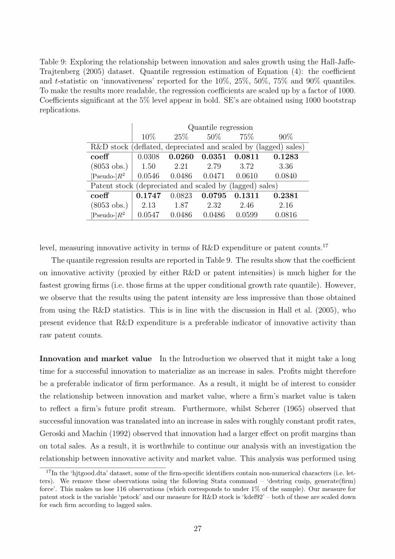
Table 9: Exploring the relationship between innovation and sales growth using the Hall-Jaffe-Trajtenberg (2005) dataset. Quantile regression estimation of Equation (4): the coefficientand t-statistic on ‘innovativeness’ reported for the 10%, 25%, 50%, 75% and 90% quantiles.To make the results more readable, the regression coefficients are scaled up by a factor of 1000.Coefficients significant at the 5% level appear in bold. SE’s are obtained using 1000 bootstrapreplications.

Quantile regression10% 25% 50% 75% 90%

R&D stock (deflated, depreciated and scaled by (lagged) sales)coeff 0.0308 0.0260 0.0351 0.0811 0.1283(8053 obs.) 1.50 2.21 2.79 3.72 3.36[Pseudo-]R2 0.0546 0.0486 0.0471 0.0610 0.0840Patent stock (depreciated and scaled by (lagged) sales)coeff 0.1747 0.0823 0.0795 0.1311 0.2381(8053 obs.) 2.13 1.87 2.32 2.46 2.16[Pseudo-]R2 0.0547 0.0486 0.0486 0.0599 0.0816

level, measuring innovative activity in terms of R&D expenditure or patent counts.17

The quantile regression results are reported in Table 9. The results show that the coefficient

on innovative activity (proxied by either R&D or patent intensities) is much higher for the

fastest growing firms (i.e. those firms at the upper conditional growth rate quantile). However,

we observe that the results using the patent intensity are less impressive than those obtained

from using the R&D statistics. This is in line with the discussion in Hall et al. (2005), who

present evidence that R&D expenditure is a preferable indicator of innovative activity than

raw patent counts.

Innovation and market value In the Introduction we observed that it might take a long

time for a successful innovation to materialize as an increase in sales. Profits might therefore

be a preferable indicator of firm performance. As a result, it might be of interest to consider

the relationship between innovation and market value, where a firm’s market value is taken

to reflect a firm’s future profit stream. Furthermore, whilst Scherer (1965) observed that

successful innovation was translated into an increase in sales with roughly constant profit rates,

Geroski and Machin (1992) observed that innovation had a larger effect on profit margins than

on total sales. As a result, it is worthwhile to continue our analysis with an investigation the

relationship between innovative activity and market value. This analysis was performed using

17In the ‘hjtgood.dta’ dataset, some of the firm-specific identifiers contain non-numerical characters (i.e. let-ters). We remove these observations using the following Stata command – ‘destring cusip, generate(firm)force’. This makes us lose 116 observations (which corresponds to under 1% of the sample). Our measure forpatent stock is the variable ‘pstock’ and our measure for R&D stock is ‘kdef92’ – both of these are scaled downfor each firm according to lagged sales.

27

0.00

1.00

2.00

3.00

4.00

inno

vativ

enes

s (s

ic 3

5)

0 .2 .4 .6 .8 1Quantile

0.00

1.00

2.00

3.00

4.00

inno

vativ

enes

s (s

ic 3

6)

0 .2 .4 .6 .8 1Quantile

−0.

100.

000.

100.

20in

nova

tiven

ess

(sic

37)

0 .2 .4 .6 .8 1Quantile

0.00

2.00

4.00

6.00

8.00

inno

vativ

enes

s (s

ic 3

8)

0 .2 .4 .6 .8 1Quantile

Figure 10: Variation in the importance of innovative activity on market value over the con-ditional quantiles of the market value distribution. Confidence intervals extend to 95% confi-dence intervals in either direction (for computational manageability, we use the Stata defaultsetting of 20 replications for the bootstrapped standard errors). Horizontal lines representOLS estimates with 95% confidence intervals. SIC 35: Machinery & Computer Equipment(top left), SIC 36: Electric/Electronic Equipment (top right), SIC 37: Transportation Equip-ment (bottom left), SIC 38: Measuring Instruments (bottom right). Graphs made using the‘grqreg’ Stata module (Azevedo 2004). Source: Coad and Rao (2006b).

a similar database and the methodology is described in detail in Coad and Rao (2006b).

The results are presented in Figure 10. We observe a similar pattern emerging as for the

case of innovation and sales growth. For the median firm, innovation has a relatively modest

influence on a firm’s market value. For the firms with the highest market value, however,

innovative activity is seen to have a much more important effect.

6 Conclusions and Implications for Policy

In modern economic thinking, innovation is ascribed a central role in the evolution of indus-

tries. In a turbulent environment characterized by powerful forces of ‘creative destruction’,

firms can nonetheless increase their chances of success by being more innovative than their

competitors. Investing in R&D is a risky activity, however, and even if an important discovery

is made it may be difficult to appropriate the returns. Firms must then combine the inven-

28

tion with manufacturing and marketing know-how in order to convert the basic ‘idea’ into a

successful product - only then will innovation lead to superior performance. The processes of

creating competitive advantage from firm-level innovation strategies are thus rather complex

and were the focus of this paper.

Nevertheless, and perhaps surprisingly, the bold conjectures on the important role of in-

novation have largely gone unquestioned. This is no doubt due to difficulties in actually

measuring innovation. Whilst variables such as patent counts or R&D expenditures do shed

light on the phenomenon of firm-level innovation, they also contain a lot of irrelevant, idiosyn-

cratic variance. In this study, innovation was measured by using Principal Component analysis

to create a synthetic ‘innovativeness’ variable for each firm in each year. This allows us to

use information on both R&D expenditure and patent statistics to extract information on the

unobserved variable of interest, i.e. ‘increases in commercially useful knowledge’, whilst dis-

carding the idiosyncratic variance of each variable taken individually. We observe that a firm,

on average, experiences only modest growth and may grow for a number of reasons that may

or may not be related to ‘innovativeness’. However, while standard regression analyses focus

on the growth of the mean firm, such techniques may be inappropriate given that growth rate

distributions are highly skewed and that high-growth firms should not be treated as outliers

but instead are objects of particular interest. Quantile regressions allows us to parsimoniously

describe the importance of innovativeness over the entire conditional growth rate distribution,

and we observed that, compared to the average firm, innovation is of great importance for the

fastest-growing firms.

In the sectors studied here, there is a great deal of technological opportunity. Competi-

tion in such sectors is organized according to the principle that a successful (and fortunate)

innovator may suddenly come up with a winning innovation and rapidly gain market share.

The reverse side of the coin, of course, is that a firm that invests in R&D but does not make a

discovery (either through missed opportunities or just plain bad luck) may rapidly forfeit its

market share to its rivals. As a result, firms in turbulent, highly innovative sectors can never

be certain how they will perform in future. Innovative firms may either succeed spectacularly

or (if they don’t happen to discover a commercially valuable innovation) they may waste a

large amount of resources, whilst their market share is threatened by more successful rivals.

This may be because they have inferior R&D capabilities or it may just be because they were

unlucky. Innovative activity is highly uncertain and although it may increase the probability

of superior performance, it cannot guarantee it. We are thus wary of innovation policies of

narrow scope that put ‘all the money on one horse’ and focus on just one or a few firms.

Instead, our results favour broad-based innovation policies that offer support to many firms

engaged in multiple directions of search, because it may not be possible to pick out ex ante

the winners from the losers.

29

We have seen that, on average, firms have a lot of discretion in their growth rates. Inno-

vation is uncertain and generally lacks persistence (Geroski, 2000; Cefis and Orsenigo, 2001);

similarly, firm growth is highly idiosyncratic and lacks persistence – inspite of this circumstan-

tial evidence, however, we should resist the temptation to overplay the relationship between

innovativeness and firm growth. On the whole, firm growth is perhaps best modelled as a

random walk (Geroski, 2000). Only a small group of highly-innovative firms are identified

and rewarded by selection pressures. Although the virtues of selective pressures operating

on heterogeneous firms have been extolled in theoretical contributions (e.g. Alchian, 1950),

it appears here that selection only wields influence over the outliers (this is in line with a

conjecture in Bottazzi et al. (2002)). Most firms, it seems, are quite oblivious to selection.

We should thus avoid the Panglossian view that unseen market forces reward the fittest and

eliminate the weakest to take the economic system to an ‘optimum’. The evidence presented

here suggests that selection is not particularly efficient (see also Coad, 2005). However, can

selection be stimulated or reinforced by intervention? This is a policy question we leave open.

We simply note here that if the ‘viability’ of firms is open to manipulation or observed with

error, the results of such intervention could be counterproductive.

Many years ago, Keynes wrote: “If human nature felt no temptation to take a chance, no

satisfaction (profit apart) in constructing a factory, a railway, a mine or a farm, there might not

be much investment merely as a result of cold calculation” (1936:150) - the same is certainly

true for R&D. Need it be reminded, an innovation strategy is even more uncertain than playing

a lottery, because it is a ‘game of chance’ in which neither the probability of winning nor the

prize can be known for sure in advance. In the face of such radical uncertainty, some firms may

well be overoptimistic (or indeed risk-averse) about what they will actually gain. For other

firms, there may be over-investment in R&D because of the ‘managerial prestige’ attached

to having an over-sized R&D department.18 As a result, we cannot rule out the possibility

that many firms invest in R&D far from something which could correspond to the ‘profit-

maximizing’ level (whatever ‘profit-maximizing’ may mean). In fact, we remain pessimistic

that R&D will ever enter into the domain of ‘rational’ decision-making (i.e. a ‘cost-benefit

analysis’). Successful innovation, and the ‘super-star’ growth performance that may result,

require risk-taking and perhaps just a little bit of craziness.

18In analogy to the principles of managerial economics, we advance that if the size of the R&D lab entersinto the R&D manager’s utility function, then investment in R&D may be far above the ‘profit-maximizing’level. Consider here the examples of the prestigious Bell Laboratories or Xerox’s renowned Palo Alto ResearchCentre, which came up with many great inventions and generated several Nobel prizes, but were unable tomake any money from these ideas (Roberts, 2004).

30

References

Aghion, P. and P. Howitt (1992), ‘A Model of Growth Through Creative Destruction’ Econo-

metrica 60 (2), 323-351.

Alchian, A.A., 1950. Uncertainty, Evolution and Economic Theory. Journal of Political Econ-

omy 58, 211-222.

Archibugi, D., 1992. Patenting as an indicator of technological innovation: a review. Science

and Public Policy 19 (6), 357-368.

Arundel, A., Kabla, I., 1998. What percentage of innovations are patented? Empirical esti-

mates for European firms. Research Policy 27, 127-141.

Azevedo, J.P.W., 2004. grqreg: Stata module to graph the coefficients of a quantile regression.

Boston College Department of Economics.

Bloom, N., Van Reenen, J., 2002. Patents, Real Options and Firm Performance. Economic

Journal 112, C97-C116.

Bottazzi, G., Dosi, G., Lippi, M., Pammolli, F., Riccaboni, M., 2001. Innovation and Cor-

porate Growth in the Evolution of the Drug Industry. International Journal of Industrial

Organization 19, 1161-1187.

Bottazzi, G., Cefis, E., Dosi, G., 2002. Corporate Growth and Industrial Structure: Some

Evidence from the Italian Manufacturing Industry. Industrial and Corporate Change 11,

705-723.

Bottazzi, G., Secchi, A., 2003. Common Properties and Sectoral Specificities in the Dynamics

of U. S. Manufacturing Companies. Review of Industrial Organization 23, 217-232.

Bottazzi, G., Coad, A., Jacoby, N., Secchi, A., 2005. Corporate Growth and Industrial Dy-

namics: Evidence from French Manufacturing. Pisa, Sant’Anna School of Advanced Studies,

LEM Working Paper Series 2005/21.

Bottazzi, G., Cefis, E., Dosi, G., Secchi, A., 2006. Invariances and Diversities in the Evolution

of Manufacturing Industries. Small Business Economics, forthcoming.

Buchinsky, M., 1994. Changes in the U.S. Wage Structure 1963-1987: Application of Quantile

Regression. Econometrica 62, 405-458.

Buchinsky, M., 1998. Recent Advances in Quantile Regression Models: A Practical Guide for

Empirical Research. Journal of Human Resources 33 (1), 88-126.

31

Carden, S.D., 2005. What global executives think about growth and risk. McKinsey Quarterly

(2), 16-25.

Cefis, E., Orsenigo, L., 2001. The persistence of innovative activities: A cross-countries and

cross-sectors comparative analysis. Research Policy 30, 1139-1158.

Coad, A., 2005. Testing the principle of ‘growth of the fitter’: the relationship between profits

and firm growth. Dept. of Economics Working Paper 05-31, Emory University, Atlanta GA.

Forthcoming in Structural Change and Economic Dynamics.

Coad, A., 2006. A Closer Look at Serial Growth Rate Correlation. Pisa, Sant’Anna School of

Advanced Studies, LEM Working Paper Series 2006/29.

Coad, A., 2007. Firm Growth: A Survey. Papers on Economics and Evolution 2007-03, Max

Planck Institute of Economics, Evolutionary Economics Group, Jena, Germany.

Coad, A., Rao, R., 2006a. Innovation and Firm Growth in ‘Complex Technology’ Sectors: A

Quantile Regression Approach. Cahiers de la Maison des Sciences Economiques No. 06050

(Serie Rouge), Universite Paris 1 Pantheon-Sorbonne, France.

Coad, A., Rao, R., 2006b. Innovation and market value: a quantile regression analysis. Eco-

nomics Bulletin 15 (13), 1-10.

Cohen, W.M., Nelson, R.R., Walsh, J.P., 2000. Protecting their intellectual assets: Appropri-

ability conditions and why US manufacturing firms patent (or not). NBER working paper

7552.

Dosi, G., 1988. Sources, Procedures, and Microeconomic Effects of Innovation. Journal of

Economic Literature 26 (3), 1120-1171.

Dunne, T., Roberts, M., Samuelson, L., 1989. The growth and failure of US Manufacturing

plants. Quarterly Journal of Economics 104 (4), 671-698.

Engelsman, E., van Raan, A.F.J., 1990. The Netherlands in Modern Technology: A Patent-

Based Assessment. Centre for Science and Technology Studies (CWTS), Leiden, The Nether-

lands; Research Report to the Ministry of Economic Affairs.

Evans, D.S., 1987. The Relationship between Firm Growth, Size and Age: Estimates for 100

Manufacturing Industries. Journal of Industrial Economics 35, 567-581.

Fizaine, F., 1968. Analyse statistique de la croissance des enterprises selon l’age et la taille.

Revue d’Economie Politique 78, 606-620.

32

Freel, M.S., 2000. Do Small Innovating Firms Outperform Non-Innovators? Small Business

Economics 14, 195-210.

Geroski, P.A., 2000. The growth of firms in theory and practice, in: Foss, N., Mahnke, V.,

(Eds.), New Directions in Economic Strategy Research. Oxford University Press, Oxford

Geroski, P. A., (2005), ‘Understanding the Implications of Empirical Work on Corporate

Growth Rates’, Managerial and Decision Economics, 26, 129-138.

Geroski, P.A., Machin, S., 1992. Do Innovating Firms Outperform Non-innovators? Business

Strategy Review, Summer, 79-90.

Geroski, P.A., Toker, S., 1996. The turnover of market leaders in UK manufacturing industry,

1979-86. International Journal of Industrial Organization 14, 141-158.

Griliches, Z., 1990. Patent Statistics as Economic Indicators: A Survey. Journal of Economic

Literature 28, 1661-1707.

Hall, B.H., 1987. The Relationship between Firm Size and Firm Growth in the U.S. Manufac-

turing Sector. Journal of Industrial Economics 35 (4), 583-600.

Hall, B.H., 2004. Exploring the Patent Explosion. Journal of Technology Transfer 30 (1-2),

35-48.

Hall, B.H., Jaffe, A., Trajtenberg, M., 2001a. Market Value and Patent Citations: A First

Look. Paper E01-304, University of California, Berkeley.

Hall, B.H., Jaffe, A., Trajtenberg, M., 2001b. The NBER Patent Citation Data File: Lessons,

Insights and Methodological Tools. NBER Working Paper 8498.

Hall, B.H., Jaffe, A., and M. Trajtenberg (2005) “Market Value and Patent Citations” Rand

Journal of Economics 36 (1), 16-38.

Hall, B. H., Lotti, F., Mairesse J., (2006) ‘Employment, Innovation, and Productivity: Evi-

dence from Italian Microdata’, mimeo, December 5.

Hall, B. H., Oriani, R., (2006) ‘Does the market value R&D investment by European firms?

Evidence from a panel of manufacturing firms in France, Germany, and Italy’ International

Journal of Industrial Organization 24 (5), 971-993.

Hair, J., Anderson, R., Tatham, R., Black, W., 1998. Multivariate Data Analysis: Fifth

Edition. Prentice Hall, Upper Saddle River, NJ.

33

Harhoff, D., Stahl, K., Woywode, M., 1998. Legal Form, Growth and Exits of West German

Firms – Empirical Results for Manufacturing, Construction, Trade and Service Industries.

Journal of Industrial Economics 46 (4), 453-488.

Harrison, R., Jaumandreu, J., Mairesse, J., Peters, B., (2005), ‘Does innovation stimulate em-

ployment? A firm-level analysis using comparable micro data on four European countries’,

mimeo, Universidad Carlos III Madrid, February.

Hart, P.E., Oulton, N., 1996. The Growth and Size of Firms. Economic Journal 106 (3),

1242-1252.

Hay, M., K. Kamshad, (1994) ‘Small Firm Growth: Intentions, Implementation and Impedi-

ments’, Business Strategy Review 5 (3), 49-68.

Holzl, W., Friesenbichler, K, (2007) ‘Are Gazelles more innovative than other firms?’, WIFO,

Austria (mimeo).

Keynes, J.M., 1936. The general theory of employment, interest, and money. MacMillan,

London.

Koenker, R., Bassett, G., 1978. Regression Quantiles. Econometrica 46, 33-50.

Koenker, R., Hallock, K.F., 2001. Quantile Regression. Journal of Economic Perspectives 15

(4), 143-156.

Lanjouw, J., Schankerman, M., 2004. Patent Quality and Research Productivity: Measuring

Innovation with Multiple Indicators. Economic Journal 114, 441-465.

Lotti, F., Santarelli E., Vivarelli, M., 2003. Does Gibrat’s Law hold among young, small firms?

Journal of Evolutionary Economics 13, 213-235.

Mansfield, E., 1962. Entry, Gibrat’s law, innovation and the growth of firms. American Eco-

nomic Review 52, 1023-1051.

Mansfield, E., Rapoport, J., Romeo, A., Villani, E., Wagner, S., Husic, F., 1977. The Produc-

tion and Application of New Industrial Technology. Norton, New York.

Marsili, O., 2001. The Anatomy and Evolution of Industries. Edward Elgar, Cheltenham.

Mosteller, F., Tukey, J., 1977. Data Analysis and Regression. Addison-Wesley, Reading, MA.

Mowery, D.C., 1983. Industrial Research and Firm Size, Survival, and Growth in American

Manufacturing, 1921-1946: An Assessment. Journal of Economic History 43 (4), 953-980.

34

Niefert, M., 2005. Patenting Behavior and Employment Growth in German Start-up Firms:

A Panel Data Analysis. Discussion Paper No 05-03, ZEW Centre for European Economic

Research, Mannheim.

OECD, 1994. Using Patent Data as Science and Technology Indicators. Patent Manual 1994,

Paris.

Roberts, J., 2004. The Modern Firm: organizational design for performance and growth.

Oxford University Press, Oxford.

Roper, S., 1997. Product Innovation and Small Business Growth: A Comparison of the Strate-

gies of German, UK and Irish Companies. Small Business Economics 9, 523-537.

Scherer, F.M., 1965. Corporate Inventive Output, Profits, and Growth. Journal of Political

Economy 73 (3), 290-297.

Stanley, M.H.R., Amaral, L.A.N., Buldyrev, S.V., Havlin, S., Leschhorn, H., Maass, P.,

Salinger, M.A., Stanley, H.E., 1996. Scaling behavior in the growth of companies. Nature

379, 804-806.

Starbuck, W. H. (1971) ‘Organizational Growth and Development’, Chapter 1 (pp. 11-141)

in W H Starbuck (Ed.), Organizational Growth and Development, Penguin modern man-

agement readings, Penguin books: Harmondsworth, UK. Originally published in 1965 as

‘Organizational Growth and Development’, pp. 451-522 in the Handbook of Organizations,

Rand McNally.

Sutton, J., 1997. Gibrat’s Legacy. Journal of Economic Literature 35, 40-59.

Van Reenen, J., 1997. Employment and Technological Innovation: Evidence from UK Manu-

facturing Firms. Journal of Labor Economics 15 (2), 255-284.

Yasar, M., Nelson, C.H., Rejesus, R.M., 2006. Productivity and Exporting Status of Manufac-

turing Firms: Evidence from Quantile Regressions. Weltwirtschaftliches Archiv, forthcom-

ing.

35