HAL Id: hal-01144855 https://hal.inria.fr/hal-01144855 Submitted on 22 Apr 2015 HAL is a multi-disciplinary open access archive for the deposit and dissemination of sci- entific research documents, whether they are pub- lished or not. The documents may come from teaching and research institutions in France or abroad, or from public or private research centers. L’archive ouverte pluridisciplinaire HAL, est destinée au dépôt et à la diffusion de documents scientifiques de niveau recherche, publiés ou non, émanant des établissements d’enseignement et de recherche français ou étrangers, des laboratoires publics ou privés. Innovative Model for Flow Governed Solid Motion based on Penalization and Aerodynamic Forces and Moments Héloïse Beaugendre, François Morency To cite this version: Héloïse Beaugendre, François Morency. Innovative Model for Flow Governed Solid Motion based on Penalization and Aerodynamic Forces and Moments. [Research Report] RR-8718, INRIA Bordeaux, équipe CARDAMOM; IMB; INRIA. 2015. <hal-01144855>
Transcript
HAL Id: hal-01144855https://hal.inria.fr/hal-01144855
Submitted on 22 Apr 2015
HAL is a multi-disciplinary open accessarchive for the deposit and dissemination of sci-entific research documents, whether they are pub-lished or not. The documents may come fromteaching and research institutions in France orabroad, or from public or private research centers.
L’archive ouverte pluridisciplinaire HAL, estdestinée au dépôt et à la diffusion de documentsscientifiques de niveau recherche, publiés ou non,émanant des établissements d’enseignement et derecherche français ou étrangers, des laboratoirespublics ou privés.
Innovative Model for Flow Governed Solid Motion basedon Penalization and Aerodynamic Forces and Moments
Héloïse Beaugendre, François Morency
To cite this version:Héloïse Beaugendre, François Morency. Innovative Model for Flow Governed Solid Motion based onPenalization and Aerodynamic Forces and Moments. [Research Report] RR-8718, INRIA Bordeaux,équipe CARDAMOM; IMB; INRIA. 2015. <hal-01144855>
Innovative Model forFlow Governed SolidMotion based onPenalization andAerodynamic Forces andMomentsHéloïse Beaugendre, François Morency
RESEARCH CENTREBORDEAUX – SUD-OUEST
200 avenue de la Vieille Tour33405 Talence Cedex
Innovative Model for Flow Governed SolidMotion based on Penalization andAerodynamic Forces and Moments
Héloïse Beaugendre∗, François Morency†
Project-Team CARDAMON
Research Report n° 8718 — Avril 2015 — 26 pages
Abstract: This work proposes a fluid-solid interaction model. It is formulated for a laminarflow modeled by the incompressible Navier-Stokes equations in which we consider the presenceof a rigid moving solid. The model is formulated inside an immersed boundary method basedon a penalization technique. The penalization technique imposes the body effects on the flow.The velocity field is extended inside the solid region and a penalty term enforces the rigid motioninside the solid region. This technique offers a great flexibility to modify the geometry of the solid.The forces and angular momentum needed for the fluid-solid interaction model are computedwith an innovative method suitable for the penalized equations method. The method is validatedsuccessfully for an oscillating airfoil in large flapping motion. Effects of different geometries onaerodynamic coefficients can then be explored. The fluid-solid interaction model is also verified forsolid motions governed by the flow, such as falling cylinder and plate.
∗ Univ. Bordeaux, IMB, UMR 5251, F-33400, Talence, France; CNRS, IMB, UMR 5251, F-33400, Talence,France; Bordeaux INP, IMB, UMR 5251, F-33400,Talence, France; INRIA, F-33400 Talence, France.† TFT Laboratory, Département de génie mécanique, École de Technologie Supérieure, Montréal, Canada
Modèle novateur pour le mouvement d’un solide entraînépar l’écoulement basé sur la pénalisation et le calcul des
forces et moments aérodynamiquesRésumé : La méthode d’interaction fluide-solide proposée dans ce rapport est formulée pour unécoulement laminaire. L’écoulement est modélisé par les équations de Navier-Stokes incompress-ibles modifiées, dans lesquelles nous considérons la présence d’un corps rigide en mouvement. Lemodèle est formulé dans le cadre d’une méthode de frontières immergées basée sur une techniquede pénalisation pour tenir compte du corps. Le champ de vitesse est étendu dans la régiondu corps rigide et un terme de pénalisation impose le mouvement rigide à l’intérieur du solide.Cette technique offre une grande souplesse pour modifier la géométrie du corps. Une méthodeinnovante appropriée pour le calcul des forces et des moments angulaires basée sur les équationspénalisées est proposée et validée pour une aile oscillante dans un grand mouvement de batte-ment. Les effets de différentes géométries peuvent ensuite être explorés. Le modèle d’interactionfluide-solide est aussi vérifié pour des mouvements de solides gouvernés par l’écoulement, commele cas d’un cylindre ou d’une plaque en chute libre.
The goal of most external flow analysis in engineering is the evaluation of aerodynamic forcesand moments. For complex flows, with massive separations for example, computational fluid dy-namics (CFD) is often the only way to reach this goal. CFD simulations are usually performedusing two types of grids: body-fitted grids and embedded grids. For body-fitted grids, externalmesh faces match up with the body surfaces and external boundary faces. On the contrary, flowsimulations by immersed boundary methods (IBM) use a grid that does not fit the body geome-try, thus avoiding most of the difficulties associated with grid generation. IBMs can easily modelflows around complex geometries in large motion [1] and are well suited for simulating complexfluid-solid interactions. The Cartesian grid, most widely used with the IBM, limits the applica-tion to Euler or Laminar flow, unless a local grid refinement strategy [2] or a specific turbulentwall model is used [3]. Methodological advances on IBM allow the simulation of compressibleflows at high Reynolds numbers [4] and therefore enable its use for aeronautic applications, suchas computation of droplet impingement [5].
As discussed by Mittal et al. in [1] and most recently by Sotiropoulos et al. in [6], IBMs canbe classified into two categories: sharp interface methods and diffused interface methods. In thefirst category the presence of boundaries is taken into account at the discrete level. The goalis to insure properties conservation closed to the boundaries and improve the accuracy at theinterface. The ghost-cell approach [4, 7, 8] belongs to this category and uses, at ghost points,values that are extrapolated from the fluid to impose the appropriate boundary conditions at theinterface. The sub-mesh penalty method [9], the immersed interface method [10] and the cut-cellmethod [11] are other approaches belonging to this class. In the second category, the diffusedinterface methods avoid the difficulties associated to the accurate tracking of the fluid-solid in-terface position. The presence of boundaries is modeled by adding a continuous forcing termdirectly to the flow equations. Immersed nodes exert a force in the momentum equations. Theeffect of immersed boundaries is distributed on surrounding nodes using delta or mask functions.Penalization method [12, 13] and its recent developments [14, 15, 16] belongs to this category.With penalization, solid bodies are represented as porous media with a very small permeability[17].
In this paper, we propose to extend the use of an IBM that combines the advantage of thepenalization and of the Vortex-in-Cell (VIC) methods [18]. The vorticity field can be seen as thesignature of bluff bodies flows. Therefore, a vorticity formulation of the Navier-Stokes equationsmay appear as the natural framework to study these flows. Since the advection of vorticity ispredominant for moderate and high Reynolds number, Lagrangian or semi-Lagrangian schemesare suitable to discretize such equations. Particle methods and VIC methods belong to this kindof approaches. Particle methods have long been used to compute vortex flows [19, 20, 21, 22].The difficulties of such methods rely on a delicate tuning of the velocity boundary conditionsespecially for complex geometries. In such sense, immersed boundary methods and especially,penalization, simplify the treatment of boundary conditions [23, 24, 25, 26]. Active researchis performed on such methods to improve their accuracy [27, 28], to increase the range of ap-plications and physical flows modelled [29], and to remain competitive in terms of computingperformances [30].
It is well known that the fluid interacts with the solid through pressure and viscous stressat the wall. However, for vorticity-based numerical simulation, the pressure distribution is notknown. The forces can be computed from the velocity and vorticity following the method pro-
RR n° 8718
4 Beaugendre & Morency
posed by Noca et al. [31], as done by Ploumhans et al. [20]. Recently, some authors haveexpressed some doubt about the validity of the forces predicted by this method for unsteadyflows when pressure and vorticity are not uniform at infinity [32]. Moreover, for vortex flowformulation, the method does not allow the computation of moments on rigid body. Eldredge[33] proposes a method to compute both forces and moment on body, based on integration alongthe surface of the vorticity derivative in the normal direction. For penalization, this method isnot easy to apply because the vorticity is not defined at the surface but rather at cartesian gridpoints near the surface. Instead, we propose an innovative forces and moment computationalmethod based on the global momentum change and angular momentum change inside the body.
The first specific objective of this paper is to propose a mathematical model for the fuid-solidinteractions within IBM. The second objective is to validate the forces and momentum calcu-lations within the VIC-IBM scheme using static and moving bodies. The flexibility offered bythe use of IBM and the level-set description of the geometries are then demonstrated. IBMs arewell suited for parametric study of geometry effects on the flow because no remeshing is neededwhen the geometry is modified [34]. The third objective is to verify the fluid-solid interactionmodel. This is done by using IBMs for the computation of flow induced body motions, such asthe free fall of a solid in a fluid [35, 36, 37]. IBMs are particularly attractive to study motion ofnon spherical bodies, such as the autorotation of flat plate [38, 39].
The paper is organized as follows, first, the penalized Navier-Stokes equations are presentedin section 2, together with the numerical method based on a VIC scheme. The new model usedto compute the forces and moment exerted by a fluid on a solid body is proposed in section 3,along with appropriate governing equations for fluid-solid interactions. In the fourth section, testcases are presented to validate forces and moments computations against literature results andexamples of fluid-solid interactions are presented.
2 Penalized Navier-Stokes equations and VIC scheme
2.1 Physical model
The fluid-solid interaction flow model proposed in this work is based on an incompressible laminarNewtonian flow around a body considered as rigid (without any deformation) and delimited bylevel-set functions. The mass and momentum conservation equations are
∇ · u = 0 in Ω (1a)∂u
∂t+ (u · ∇) u− ν∇2u +
1
ρ∇p = 0 in Ω. (1b)
where u is the velocity vector, ν = µ/ρ is the kinematic viscosity, ρ is the density, and p is thepressure. Now we consider, in Ω, the presence of a rigid moving solid Si. The boundary of Si
is computed from a level set function Φsi . Φsi is the signed distance function to Si, typicallyΦsi will be negative inside the object and positive outside, see figure 1 for an illustration of thesigned distance function, embedded into a Cartesian grid, corresponding to a wing and an icedebris.
The penalization technique extends the velocity field inside the solid body, as illustrated infigure (2), and solve the flow equations with a penalty term to enforce rigid motion inside thesolid as proposed by [24]. Let usi be the rigid moving body velocity vector of Si. Inside Si, themomentum equation becomes u = usi and remains equation (1b) outside Si.
Inria
Computation of Aerodynamic Forces and Moments 5
Figure 1: Global level-set function of two rigid bodies (wing and ice debris) computed onto aCartesian grid.
This is summarized as follows: given a very large penalization parameter, λ 1, and denotingby χsi the characteristic function of the solid Si, i.e. χsi = 1 inside Si and χsi = 0 outside Si,the penalized Navier-Stokes equations are
∂u
∂t+ (u · ∇) u− ν∇2u +
1
ρ∇p = λχsi(usi − u) for x ∈ Ω and t > 0, (2)
coupled with the incompressible mass conservation (1a). This model can easily be generalizedto multiple rigid bodies Si.
To solve our governing equations the following strategies have been chosen:
1. A vortex formulation of our governing equations is used: this formulation is especially welladapted to study oscillatory motions that create large flow separation around aerodynamicbodies.
2. A vortex in cell (VIC) scheme is used to solve the obtained equations: this scheme offersless CFL restrictions than classical schemes.
3. A time splitting algorithm allows to take into account the specific requirement of eachequation term, for example the implicit treatment of the penalization term for accuracypurpose.
Let us give more precision on each choice previously described.
RR n° 8718
6 Beaugendre & Morency
Figure 2: Penalization technique, the flow field is extended inside the bodies, u component ofthe velocity, v component of the velocity and vorticity.
Inria
Computation of Aerodynamic Forces and Moments 7
2.2 Vortex formulation
Let us consider the penalized Navier-Stokes equation in the vorticity formulation by applyingthe curl operator to equation (2), with ω = ∇× u in Ω
∂ω
∂t+ (u · ∇)ω = (ω · ∇) u + ν∇2ω + λ∇× [H(Φsi)(usi − u)] (3)
with ∇ · u = 0 in Ω . (4)
In equation (3), χsi = H(Φsi), where H is the Heaviside function. In this paper, the vorticityfield is numerically determined by a particle discretization using the scheme presented in thenext section. Because the equations are not written in primitive variables, special treatmentsare needed to recover the velocity field and to impose the boundary conditions. Since theincompressible velocity field is divergence-free, from the vector field theory, we can define avector potential Ψ such that
u = ∇×Ψ . (5)
This potential vector is imposed to be solenoidal, that is ∇ ·Ψ = 0, and given ω the updatedvorticity field, the stream function field is computed by solving the linear Poisson equation,
∆Ψ = −ω, (6)
on the cartesian grid with boundary conditions on ∂Ω, using a Fast Fourier Transform (FFT)solver.
2.3 VIC scheme
The Vortex-In-Cell (VIC) scheme computes the non linear advection by tracking the trajectoriesof Lagrangian particles through a set of ODEs. An Eulerian grid is adopted to solve the velocityfield, the diffusive term, and the penalization term. Given D/Dt(·), the material derivative,equation (3) becomes
Dω
Dt= (ω · ∇) u + ν∇2ω + λ∇× [H(Φsi)(usi − u)] (7)
The domain Ω is meshed using a uniform fixed cartesian grid. We denote the time step ∆t,such that tn = n∆t and Φn
si , un, ωn are grid values of the level set functions, velocity, andvorticity. The vorticity field ω is represented by a set of particles
ω(x) =
N∑p=1
vpωpζ (x− xp) , (8)
where N is the number of particles, xp the particle location, vp and ωp are the volume and thestrength of a general particle p. ζ is a smooth distribution function, such that
∫ζ(x) dx = 1,
which acts on the vortex support. In vortex methods, the rate of change of vorticity is modeled bymeans of discrete vortex particles, such that the solution of (7) is localized only in the rotationalregions of the flow field. This is the most important advantage of the vortex methods, that is,the computational efforts are naturally addressed only to specific flow field zones.
RR n° 8718
8 Beaugendre & Morency
2.4 Splitting algorithmA viscous splitting algorithm solves the equation (3). Each time step ∆t is solved using threesub-steps as follows.
1−Advection:Dω
Dt=∂ω
∂t+ (u · ∇)ω = 0. (9a)
2− Stretching and diffusion:∂ω
∂t= (ω · ∇) u + ν∇2ω. (9b)
3− Penalization term:∂ω
∂t= λ∇× (H (Φsi) (usi − u)) . (9c)
sub-step 1: advectionStarting with ωn, grid vorticity above a certain cut-off value will create particles at grid pointlocations [40], figure 3 a). Then, using equation (9a), particles are displaced with a fourth orderRunge-Kutta time-stepping scheme, figure 3 b). From the new vortex particles’ location, thevorticity field is remeshed on the grid, ω?, by the M ′4 third order interpolation kernel introducedby [41], figure 3 c).
Figure 3: Particles interpolation scheme. The circle’s size denotes the strenght of the particle and thesolid circles represent the advected particles. a) vortex particles and velocity field; b) advection step; c)remesh-diffusion step.
sub-step 2: stretching and diffusionThe equation to solve for vortex stretching and viscous contribution is given by equation (9b)applied to ω?. This equation is approximated onto the grid with an Euler explicit scheme, whilethe Laplacian is evaluated with a second order accurate standard five points stencil. The resultsis noted ω??.
sub-step 3: penalizationThe penalization term is evaluated using equation (9c). In our simulations, λ is fixed to 108/∆t.An implicit Euler time discretization is used to approximate un+1 in the penalization term:
un+1 =u?? + λ∆tH(Φsi)u
nsi
1 + λ∆tH(Φsi). (10)
where u?? is the velocity computed using ω?? resulting of sub-step 2 (∆Ψ?? = −ω?? and u?? =∇ ×Ψ?? ). The vorticity field at tn+1 is then evaluated on the grid by taking the curl of thevelocity, ωn+1 = ∇ × un+1, and computing the derivative through the second order centeredfinite differences approximation. This method is unconditionally stable and enables to take avery large penalization parameter to insure accuracy.
Inria
Computation of Aerodynamic Forces and Moments 9
3 Aerodynamic forces and moment computations and fluid-solid interaction model
The penalization term in equation (3), the last term on the right hand side, can also be consideredas being the rigid body effect on fluid. At each time step, the penalization term forces the velocityinside the rigid body Si to be equal to usi . In velocity formulation, the local momentum changeimposed by the penalization is computed by
∂u
∂t= λH(Φsi)(usi − u) (11)
In our formulation, the velocity u is implicitly calculated by (10). Thus, the penalization termbecome
∂u
∂t= λH(Φsi)
(unsi −
(u?? + λ∆tH(Φsi)u
nsi
1 + λ∆tH(Φsi)
))(12)
∂u
∂t= λH(Φsi)
(unsi(1 + λ∆tH(Φsi))− (u?? + λ∆tH(Φsi)u
nsi)
1 + λ∆tH(Φsi)
)(13)
∂u
∂t= λH(Φsi)
(unsi − u??
1 + λ∆tH(Φsi)
). (14)
The global momentum change is obtained by integration over the computational solid domainSi and the forces are defined as
F =
∫Si
ρfλH(Φsi)
1 + λ∆tH(Φsi)(un
si − u??)dx. (15)
In a similar way, the angular momentum change created by the penalization term requiresan integration over the solid domain Si and the instantaneous pitching moment is defined by
T =
∫Si
ρfλH(Φsi)
1 + λ∆tH(Φsi)r× (un
si − u?)dx. (16)
In 2D flows, the drag, lift and pitching moment coefficients are defined respectively as
CX =Fx
1/2ρfU2∞c
CY =Fy
1/2ρfU2∞c
Cm =T
1/2ρfU2∞c
2. (17)
where the x axis is aligned with the far field velocity vector U∞, the y axis is perpendicular tothe far field velocity vector and c is the airfoil chord. For an imposed motion of the solid Si,given usi we compute the aerodynamic coefficients given by equation (17).
The model for fluid-solid interaction is different from the one used in the previous paper [42].For a fluid-solid interaction the forces acting on the solid Si induce its motion, the governingequations are then given by
∂usi
∂t=
F
Ma+
(ρsi − ρf )
ρsiG (18)
∂θ
∂t=
T
Mi(19)
where Ma is the mass of the solid Si, Mi its moment of inertia, ρsi its density, ρf the fluiddensity and G the gravity vector. The formalism can be easily extended to multiple solids.
RR n° 8718
10 Beaugendre & Morency
Table 1: Static cylinder, values of mean CD
(CD
)and St obtained at Re=150 with three different
gridsh Methods CD St
1/128 Noca 1.475 0.173Momentum 1.523 0.173
1/256 Noca 1.381 0.173Momentum 1.386 0.172
1/512 Noca 1.347 0.173Momentum 1.356 0.173
4 Numerical resultsIn this section, forces and moments computations are validated using a static cylinder and anoscillating flapping wing motion. Examples of fluid-solid interactions are presented to show thecapabilities of the IBM.
4.1 Static cylinder test caseThe computations are done on a square domain of size [−1.85, 6.15]× [−4, 4]. The centre of thecylinder, whose diameter D is 0.3, is at (0, 0). The far field velocity is U∞ = 1. The fluid viscosityis selected to achieve the desired Reynolds number Re = 150. The potential flow solution arounda cylinder defines reliable values of the flow field at domain boundaries. For example, on the topand bottom boundaries a Dirichlet condition is enforced. That is
Ψ = U∞y
(1− (D/2)2
x2 + y2
)top, bottom. (20)
This is equivalent to impose a symmetry condition on top and bottom boundaries. Neumannboundary conditions are imposed at upstream and downstream locations, that is
∂Ψ
∂x=
2U∞(D/2)2xy
(x2 + y2)2upstream, downstream. (21)
Three meshes with h = 1/128, 1/256 and h = 1/512, where h is the grid spacing, are usedfor computations. The time step dt for computation is evaluated by
dt = (0.5h)2Re (22)
where the Reynolds number is defined as Re = U∞D/ν.Table 1 compares some results obtained with the three meshes to evaluate grid sensitivities of
the results. The forces Fx and Fy are obtained with the Noca formulation [31] and Momentumformulation equation (15). The mean drag coefficient CD, CX averaged over one period and theStrouhal number St are tabulated. The St value depends on the shedding frequency f or on thedimensionless time period Tp
St =fD
U∞= 1/Tp .
Inria
Computation of Aerodynamic Forces and Moments 11
The dimensionless time period is evaluated by looking at the lift coefficient, CY , evolution intime. For three significant digits, the St values do not depend on the force formulation or onthe mesh size. It is expected that for a fine enough mesh, the two formulations should give thesame results. The average mean drag coefficient values are between the values of 1.44 from Laiand Peskin [43] and 1.334 from Liu al. [44]. The Strouhal number are close to the value of 0.184computed in [43].
4.2 Validation of forces through an oscillating airfoilFlapping wing motions are extensively studied for engineering applications in low Reynolds num-bers flow where classical fixed wing geometry performance decreases, [45]. According to previousworks, around ten parameters influence the power extraction in flapping wing motions, such asoscillation frequencies and amplitudes (translational and rotational), phase difference betweenplunge and pitch motion, viscosity, free stream velocity, flapping pattern and airfoil geometry. Inthis section, we will study the effect of the pitching position and of the geometry’s shape, afterthe validation of unsteady forces calculations.
For validation, an oscillating airfoil experiencing simultaneous pitching θ(t) and heaving h(t)motions is modelled. The infinitely long wing is based on a NACA 0015 airfoil. The pitching axisis located along the airfoil chord at the position (xp, yp) = (1/3, 0). The airfoil motion, describedby Kinsey and Dumas [46], is defined by the heaving h(t) and the pitching angle θ(t) as follows
h(t) = H0 sin (ωt+ Φ)θ(t) = θ0 sin (ωt)
(23)
where H0 is the heaving amplitude and θ0 is the pitching amplitude. The angular frequency isdefined by ω = 2πf and the phase difference Φ is set to 90o. The heaving velocity is then givenby
Vy(t) = H0ω cos(ωt+ Φ) . (24)
Based on the imposed motion and on the upstream flow conditions, the airfoil experiences aneffective angle of attack α(t) and an effective upstream velocity Veff (t) defined by
α(t) = arctan(−Vy(t)/U∞)− θ(t)Veff (t) =
√(U2∞ + V 2
y (t)),
(25)
where the freestream velocity far upstream of the oscillating airfoil is U∞ = 1.
To validate our simulations, a regime corresponding to the parameters Re =U∞c
ν= 1100,
H0/c = 1, f = 0.14, xp/c = 1/3 and θ0 = 76.33o has been computed. A view of the motion issketched in figure 4. Our numerical results, obtained using dx = dy = 1 × 10⁻³, dt = 5 × 10⁻⁴
and λ = 1 × 10⁸, are then compared to the forces predictions presented by Kinsey et al. [46]and by Campobasso et al. [47]. Results of instantaneous forces, equation (17), CX , CY andpitching moments Cm, figure 5, are in good agreements with literature results. Our solutionslightly overestimates the drag coefficient amplitude and the minimum/maximum of the liftcoefficient but correctly predicts the curve shape of those coefficients. The momentum coefficientis correctly predicted as well, our curve is slightly shifted to the left compared to literature results(corresponding to a time lag), figure (5c).
RR n° 8718
12 Beaugendre & Morency
X
Y
0.5 0 0.5 1 1.5
1
0.5
0
0.5
1
Figure 4: Oscillating airfoil, sketch of the airfoil motion for H0/c = 1, f = 0.14, xp/c = 1/3 andθ0 = 76.33o.
A mesh sensitivity study using different mesh sizes and different domain sizes has been per-formed to verify the sensibility of the force predictions. All the simulations used the same timestep fixed to dt = 5× 10⁻⁴. Figures 6 (a), (b) and (c) compare CX , CY and Cm obtained withthree different meshes corresponding to a coarse mesh dx = dy = 5 × 10⁻³, a medium meshdx = dy = 2× 10⁻³ and a fine mesh dx = dy = 1× 10⁻³ and demonstrate the consistency of themethod. Each mesh allows to compute a good approximation of the forces and moment evolutionthrough a time period. As the mesh becomes finer the solution converges to the solution obtainedon the finest mesh.Simulations using the medium grid scale dx = dy = 2 × 10⁻³ and two different domains, onedomain of size [−3, 8] × [−4, 4] referenced as dom1 and the other one of size [−3, 8] × [−6, 6]referenced as dom2, have also been performed to investigate boundary conditions effects andmore especially blocking effects on the solution. Figure 6 (d) demonstrates that a small blockingeffect is observable on this test case. Indeed, reducing slightly the height of the domain leads toan amplitude increase of the CX coefficient. Since the comparisons with the literature resultshave been done on the smallest domain, the blocking effects are most probably responsible of theoverestimation noticed on the CX curve. However, even the coarse mesh on the small domainexhibits the correct behavior of the solution. The following studies are then performed using thesmallest domain and the medium grid scale to ensure a good compromise between the quality ofthe solution and cpu time.
4.3 Flexibility offered by penalization
Penalization technique offers a simple way to consider different geometries for the solid Si becausethe same mesh can be used for all simulations. To illustrate this capability of the method threekind of geometries have been selected. The NACA 0015 profile, a rounded edge rectangular platewith a ratio chord/thickness = 15% and a NACA 0040 profile. Those geometries are sketchedon figure (7a). The method enables also to easily modify the position of the pitching axis, thustwo different positions have been selected (xp, yp) = (1/3, 0) and (xp, yp) = (1/2, 0). Thosegeometries evolve using the same motion as described in section 4.2.
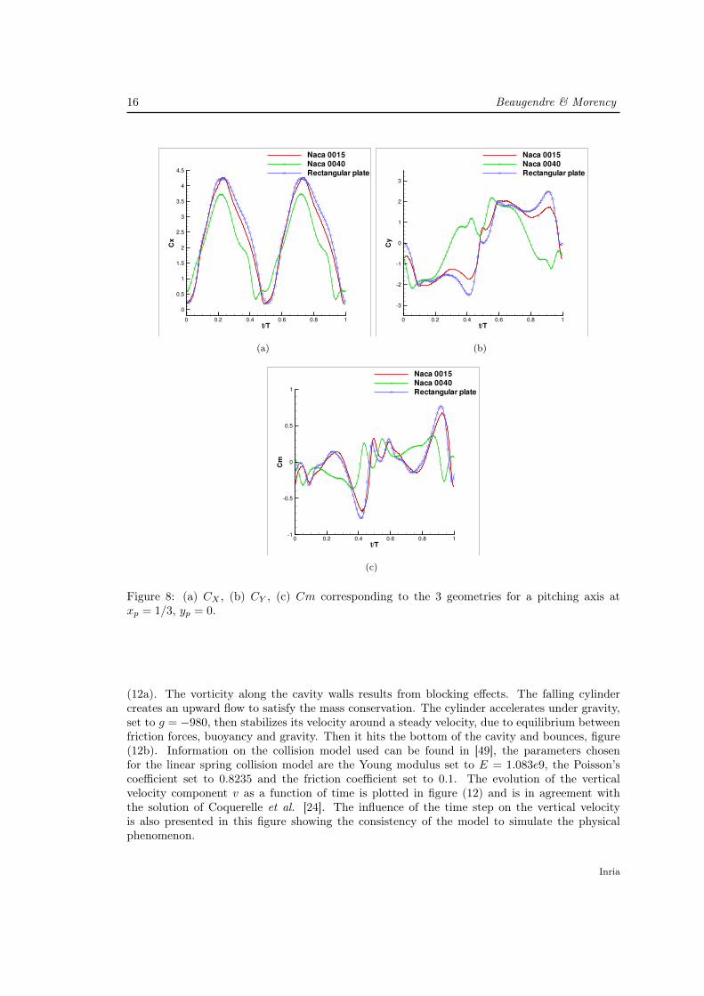
For the first position of the pitching axis (1/3, 0), the motion of tow of the three geometriesis sketched on figures 4 & 7(b). Figure (8) compares CX , CY and Cm for the three geometries.
Inria
Computation of Aerodynamic Forces and Moments 13
t/T
Cx
0 0.2 0.4 0.6 0.8 1
0
0.5
1
1.5
2
2.5
3
3.5
4
4.5
dx=dy=1.d3Kinsey
Campobasso
(a)
t/T
Cy
0 0.2 0.4 0.6 0.8 1
2
1
0
1
2
dx=dy=1.d3
Kinsey
Campobasso
(b)
t/T
Cm
0 0.2 0.4 0.6 0.8 11
0.5
0
0.5
1
dx=dy=1.d3
Kinsey
Campobasso
(c)
Figure 5: Oscillating airfoil, comparison with the results obtained by Kinsey et al.[46] andCampobasso et al. [47] (a) Drag coefficient, (b) Lift coefficient, (c) Pitching moment.
As expected for such a low Reynolds number flow the results obtained with the NACA 0015airfoil and the rectangular plate of the same thickness are very similar. The thicker airfoil onthe contrary exhibits a different behavior. As in the work done by Ashraf al. [48], depending onthe Reynolds number, flow around thicker flapping airfoils can be radically different than flowaround thin geometries. Indeed, results of the mean power, table (2), show that thin geometriesextract 1.5 to 3 times more power than thick geometry. The instantaneous power results fromthe sum of the heaving contribution FyVy(t) and the pitching contribution Tθ(t), where T is theresulting torque about the pitching axis xp. The mean power extracted over one cycle can thusbe computed using equation (26).
Cpower =Ppower12ρU
3∞c
RR n° 8718
14 Beaugendre & Morency
t/T
Cx
0 0.2 0.4 0.6 0.8 10.5
0
0.5
1
1.5
2
2.5
3
3.5
4
4.5
dx=dy=1.d3
dx=dy=2.d3
dx=dy=5.d3
(a)
t/T
Cy
0 0.2 0.4 0.6 0.8 1
2
0
2
dx=dy=1.d3
dx=dy=2.d3
dx=dy=5.d3
(b)
t/T
Cm
0 0.2 0.4 0.6 0.8 11
0.5
0
0.5
1
dx=dy=1.d3dx=dy=2.d3
dx=dy=5.d3
(c)
t/T
Cx,C
y,C
m
0 0.2 0.4 0.6 0.8 1
2
0
2
4
dom1
dom2
(d)
Figure 6: Mesh sensitivity on the drag coefficient (a) on the lift coefficient (b) and on the pitchingmoment (c). For the medium mesh, dx = dy = 2×10⁻³ influence of the domain size on calculatedforces and moment, dom1 = [−3, 8]× [−4, 4], dom2=[−3, 8]× [−6, 6].
Cpower =
∫ 1
0
(CY (t)
Vy(t)
U∞+ Cm(t)
θ(t)c
U∞
)dt. (26)
Moving the pitching position from the leading edge to the middle of the wing increases the meanpower extracted for the thick airfoil and on the contrary decreases the mean power for thingeometries, table 2.
The results related to the motion corresponding to the second pitching axis location (xp, yp) =(1/2, 0) are presented in figures (10) and (11). First, the motion using this pitching axis loactionis sketched in figure (9). Figure (10) compares the evolution over one cycle of CX , CY and Cm forthe three geometries. Again the NACA 0015 airfoil and the rectangular plate exhibit comparablebehaviors, the curves evolving with a similar pattern. The thick airfoil results remain different.
The modification of the pitching axis position reduces the CX coefficient for the three ge-ometries, figures (11a-d-g). The pitching moment coefficient become antisymmetric as expectedthanks to the symmetry of the motion, figures (11c-f-i). For thin geometries, the modification ofthe pitching location leads to related modification of the curves. CX , CY and Cm curves from
Inria
Computation of Aerodynamic Forces and Moments 15
X
Y
0 0.2 0.4 0.6 0.8 1
0.2
0
0.2
0.4
0.6
Naca 0015
Naca 0040
Rectangular plate
(a)
X
Y
1 0.5 0 0.5 1 1.5
1
0.5
0
0.5
1
(b)
Figure 7: a) Geometries of the NACA 0015 profile, NACA 0040 profile and the rectangular plate.b) Motion of the rectangular plate for a pitching position at xp = 1/3, yp = 0.
Table 2: Mean Cpower for the three geometries and the two axis pitching positionGeometry (xp, yp) = (1/3, 0) (xp, yp) = (1/2, 0)NACA 0015 0.945 0.830NACA 0040 0.339 0.625
Rectangular plate 1.043 0.830
figures (11a and d), (b and e) and (c and f) respectively look similar. The flow around the thickairfoil seems more affected by the position of the pitching axis, figures(11g-h-i).
4.4 Fluid-solid interaction
In this sub-section, trajectories of objects are computed using the proposed fluid-solid interactionmodel. We will first validate our model against a 2D falling cylinder to compare with literatureresults. Then we will use the rectangular plate described previously to study the effects of densityratios on the trajectories.
4.4.1 Falling cylinder
This test case is representative of the sedimentation of a 2D cylinder on a flat plate. We considerthe case of a 2D cylinder in a square cavity, falling under gravity on a flat plane. The dimensionof the cavity is [0, 2] × [0, 6]. The viscosity is 0.01. The density inside and outside the cylinderis, respectively, 1.5 and 1. The mesh spacing is dx = dy = 3.9× 10⁻³.The cylinder has a radiusof 0.125, no roughness, and its barycenter is initially located at the point (1,4). To impose wallboundary conditions on each wall of the cavity we use a penalization layer of 10 cells all aroundthe cavity, this is the reason why the domain, in figure (12a) appears slightly larger and longerthan the cavity definition. A snapshot of the vorticity field, at time t = 0.3, is depicted in figure
RR n° 8718
16 Beaugendre & Morency
t/T
Cx
0 0.2 0.4 0.6 0.8 1
0
0.5
1
1.5
2
2.5
3
3.5
4
4.5
Naca 0015
Naca 0040
Rectangular plate
(a)
t/T
Cy
0 0.2 0.4 0.6 0.8 1
3
2
1
0
1
2
3
Naca 0015
Naca 0040
Rectangular plate
(b)
t/T
Cm
0 0.2 0.4 0.6 0.8 11
0.5
0
0.5
1
Naca 0015
Naca 0040
Rectangular plate
(c)
Figure 8: (a) CX , (b) CY , (c) Cm corresponding to the 3 geometries for a pitching axis atxp = 1/3, yp = 0.
(12a). The vorticity along the cavity walls results from blocking effects. The falling cylindercreates an upward flow to satisfy the mass conservation. The cylinder accelerates under gravity,set to g = −980, then stabilizes its velocity around a steady velocity, due to equilibrium betweenfriction forces, buoyancy and gravity. Then it hits the bottom of the cavity and bounces, figure(12b). Information on the collision model used can be found in [49], the parameters chosenfor the linear spring collision model are the Young modulus set to E = 1.083e9, the Poisson’scoefficient set to 0.8235 and the friction coefficient set to 0.1. The evolution of the verticalvelocity component v as a function of time is plotted in figure (12) and is in agreement withthe solution of Coquerelle et al. [24]. The influence of the time step on the vertical velocityis also presented in this figure showing the consistency of the model to simulate the physicalphenomenon.
Inria
Computation of Aerodynamic Forces and Moments 17
X
Y
0.5 0 0.5 1 1.5 2
1.2
1
0.8
0.6
0.4
0.2
0
0.2
0.4
0.6
0.8
1
1.2
(a)
X
Y
0.5 0 0.5 1 1.5 2
1.2
1
0.8
0.6
0.4
0.2
0
0.2
0.4
0.6
0.8
1
1.2
(b)
Figure 9: Motion of the geometries for a pitching position at xp = 1/2, yp = 0.
4.4.2 Falling rectangular plate
We use the previous rectangular plate, from sub-section 4.3 for which the gravity center of theplate is positionned at (0, 0) with a rotation angle of attack of π/3 with the horizontal axis, thecomputational domain is set to [−3, 8] × [−4, 4]. First we compute the flow motion around thefixed rectangular plate. The Reynolds number is set at Re = 1100 as in the previous studyusing this solid body, see section 4.3. A snapshot of the vorticity field around the fixed plate ispresented in figure (13). At time t = 0.5, the fluid-solid interaction is started. Once the fluid-solidinteraction occurs, the aerodynamic forces and moment acting on the solid induce its motion.During these simulations, the pivot axis of the rectangular plate coincides with its barycenter.The first simulations consist in investigating the sensitivity of the trajectory according to themesh. In those simulations ρs = ρf and the time step dt is fixed to 5 × 10⁻⁴. Figure (14a)presents the position of the plate every 400 steps using 5 meshes. The plate trajectory is verystable according to the grid size. As can be seen through figures (14b-d) the evolution in time ofthe velocities (u-component, v-component and angular velocity) is similar. The velocities valueevolves smoothly from the coarser mesh to the finer mesh. The angle of rotation with the initialposition, figure (14d) induce a similar motion of the plate for all the meshes. The range of thetrajectory and the reactivity of the rectangular plate to the flow is slightly affected by the gridsize.
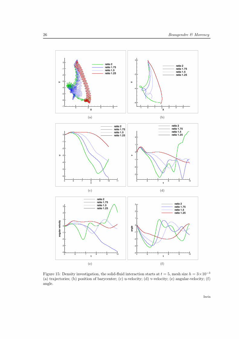
To verify the influence of plate’s density on the trajectory, four density ratios have been se-lected ρs/ρf = 2; 1.75; 1.5 and 1.25. The simulations have been performed using the mediummesh dx = dy = 3.×10−3 with a time step of dt = 5×10⁻⁴ and a domain of [−3, 5]× [−9, 3]. Asexpected, from previous work in literature [35], the plate starts to auto-rotate, figure (15a). Theauto-rotation starts sooner for larger density ratio. Again, figure (15a), shows the position of theplate every 400 time steps for each density ratio. The falling velocity, v (figure 15d), of the plateincreases with the plate weight. The vertical acceleration of the plate destabilizes its orientationand the plate starts to rotate around its barycenter axis, figure (15e). The modification of theplate orientation with the flow reduces the falling velocity (the gravity force is compensated bybuoyancy and aerodynamic forces), figure (15d). Due to its initial orientation and its weight,at the beginning of the fluid-solid interaction, the plate glides to the left (figures 15b & c). Asexpected, the lighter plate is more affected by the flow and is pushed to the right by the flow.
RR n° 8718
18 Beaugendre & Morency
t/T
Cx
0 0.2 0.4 0.6 0.8 1
0
0.5
1
1.5
2
2.5
3
3.5
4
4.5
Naca 0015
Naca 0040
Rectangular plate
(a)
t/T
Cy
0 0.2 0.4 0.6 0.8 1
3
2
1
0
1
2
3
Naca 0015
Naca 0040
Rectangular plate
(b)
t/T
Cm
0 0.2 0.4 0.6 0.8 11
0.5
0
0.5
1
Naca 0015
Naca 0040
Rectangular plate
(c)
Figure 10: (a) CX , (b) CY , (c) Cm corresponding to the 3 geometries for a pitching position atxp = 1/2, yp = 0.
For the cylinder and the rectangular plate test cases the fluid-solid interaction model behavesconsistently for varying density ratio, mesh size and time step.
5 Conclusions
This paper has presented an original way of computing aerodynamic forces and moments alongwith the governing equations to use them in order to simulate fluid-solid interactions. Forcesand moments have been validated within the VIC-IBM scheme using static and dynamic bodies.Predicted forces and moment agree with literature for a static cylinder and a flapping wing mo-tion. The flexibility offered by the use of IBM and the level-set description of the geometries hasbeen demonstrated. The fluid-solid interaction model has been compared to another approachfor a falling cylinder test case and the falling velocity agrees with literature results. For varying
density ratio, mesh size and time step, the fluid-solid interaction model predicts realistic trajec-tories for a rectangular plate. Further experimental results are needed to properly validate thismodel. Since aeronautic applications will be considered with the computation of ice sheddingtrajectories a specific turbulent wall model is under development.
6 Ackowledgement
Numerical experiments presented in this paper were carried out using the PLaFRIM experimentaltestbed and the BOREAS cluster. BOREAS cluster is funded by the Natural Sciences and Engi-neering Research Council of Canada. PLaFRIM cluster being developed under the Inria PlaFRIM
RR n° 8718
20 Beaugendre & Morency
(a)
t
V
0 0.1 0.2 0.3 0.4 0.5 0.6
15
10
5
0
5
Coquerelle
dt=5.d4
dt=1.d4
dt=5.d5
(b)
Figure 12: Sedimentation of a 2D falling cylinder. a) Vorticity field at time t = 0.3. b) Sensitivityof the solution against the time step and comparison against Coquerelle’s velocity profile [24] .
development action with support from LABRI and IMB and other entities: Conseil Régional dAquitaine, FeDER, Université de Bordeaux and CNRS, see https://plafrim.bordeaux.inria.fr/).
References
References
[1] R. Mittal, G. Iaccarino, Immersed boundary methods, Annu. Rev. Fluid. Mech. 37 (2005)239–261.
[2] J. T. Rasmussen, G. H. Cottet, J. H. Walther, A multiresolution remeshed vortex-in-cellalgorithm using patches, Journal of Computational Physics 230 (2011) 6742–6755.
Inria
Computation of Aerodynamic Forces and Moments 21
(a)
Figure 13: Solution around the static rectangular plate, vorticity contours (negative in blue;positive in red).
[3] F. Capizzano, Turbulent wall model for immersed boundary methods, AIAA Journal 49 (11).
[4] R. Ghias, R. Mittal, H. Dong, A sharp interface immersed boundary method for compressibleviscous flows, Journal of Computational Physics 225 (2007) 528–553.
[5] F. Capizzano, E. Iuliano, A eulerian method for water droplet impingement by means ofan immersed boundary technique, Journal of Fluids Engineering-Transactions of the Asme136 (4).
[6] F. Sotiropoulos, X. L. Yang, Immersed boundary methods for simulating fluid-structureinteraction, Progress in Aerospace Sciences 65 (2014) 1–21.
[7] F. Tseng, A ghost cell immersed boundary method for flow in complex geometry, Journalof Computational Physics 192 (2003) 593–623.
[8] Y. Gorsse, A. Iollo, H. Telib, L. Weynans, A simple second order cartesian scheme forcompressible euler flows, Journal of Computational Physics 231 (2012) 7780–7794.
[9] A. Sarthou, S. Vincent, P. Angot, J. Caltagirone, The sub-mesh penalty method, Finite Vol.Complex Appl. V (2008) 633–640.
[10] M. Linnick, H. Fasel, A high order interface method for simulating unsteady incompressibleflows on irregular domains, Journal of Computational Physics 204 (2005) 157–192.
[11] P. Collela, D. Graves, B. Keen, D. Modiano, A cartesian grid embedded boundary methodfor hyperbolic conservation laws, Journal of Computational Physics 211 (2006) 347–366.
[12] P. Angot, C. Bruneau, P. Fabrie, A penalization method to take into account obstacles inincompressible viscous flows, Numerische Mathematik 81 (4) (1999) 497–520.
[13] E. Arquis, J. Caltagirone, Sur les conditions hydrodynamiques au voisinage d’une interfacemilieu fluide-milieux poreux: application à la convection naturelle, C.R. Acad. Sci. Paris II299 (1984) 1–4.
RR n° 8718
22 Beaugendre & Morency
[14] M. Bergmann, A. Iollo, Modeling and simulation of fish-like swimming, Journal of Compu-tational Physics 230 (2) (2011) 329–348.
[15] O. Boiron, G. Chiavassa, R. Donat, A high-resolution penalization method for large machnumber flows in the presence of obstacles, Comput. Fluids 38 (3) (2009) 703–714.
[16] R. Abgrall, H. Beaugendre, C. Dobrzynski, An immersed boundary method using unstruc-tured anisotropic mesh adaptation combined with level-sets and penalization techniques,Journal of Computational Physics 257 (2014) 83–101.
[17] B. Kadoch, D. Kolomenskiy, P. Angot, K. Schneider, A volume penalization method forincompressible flows and scalar advection-diffusion with moving obstacle, Journal of Com-putational Physics 231 (2012) 4365–4383.
[18] F. Morency, H. Beaugendre, F. Gallizio, Aerodynamic force evaluation for ice sheddingphenomenon using vortex in cell scheme, penalisation and level set approaches, InternationalJournal of Computational Fluid Dynamics 26 (9-10) (2012) 435–450.
[19] P. Koumoutsakos, A. Leonard, High-resolution simulations of the flow around an impulsivestarted cylinder using vortex methods, Journal of Fluid Mechanics 296 (1995) 1–38.
[20] P. Ploumhans, G. S. Winckelmans, J. K. Salmon, A. Leonard, M. S. Warren, Vortex methodsfor direct numerical simulation of three-dimensional bluff body flows: application to thesphere at re = 300, 500, and 1000, Journal of Computational Physics 178 (2) (2002) 427–463.
[21] G. Cottet, P. Koumoutsakos, Vortex methods: theory and practice, Cambridge Univ Pr,2000.
[22] G. Cottet, P. Poncet, Advances in direct numerical simulation of 3d wall-bounded flows byvortex-in-cell methods, Journal of Computational Physics 193 (2003) 136–158.
[23] N. Kevlahan, J. Ghidaglia, Computation of turbulent flow past an array of cylinders usinga spectral method with brinkman penalization, Eur. J. Mech. B20 (2001) 333–350.
[24] M. Coquerelle, G. Cottet, A vortex level set method for the two-way coupling of an incom-pressible fluid with colliding rigid bodies, Journal of Computational Physics 227 (21) (2008)9121–9137.
[25] C. Mimeau, I. Mortazavi, G. Cottet, Passive flow control around a semi-circular cylinderusing porous coatings, Int. Journal of flow control 6 (1) (2014) 43–60.
[26] C. Mimeau, F. Gallizio, G. Cottet, I. Mortazavi, Vortex penalization method for bluff bodyflows, submitted to Int. Jour. for Num. Meth. in Fluids.
[27] M. Gazzola, B. Hejazialhosseini, P. Koumoutsakos, Reinforcement learning and weveletadapted vortex methods for simualtions of self-propelled swimmers, SIAM J. Sci. Comput.36 (3) (2014) B622–B639.
[28] G. Cottet, J.-M. Etancelin, F. Perignon, C. Picard, High order semi-lagrangian particles fortransport equations : numerical analysis and implementation issues, ESAIM: MathematicalModelling and Numerical Analysis 48 (2014) 1029–1064.
[29] J. Rasmussen, G. Cottet, J. Waltherw, A multiresolution remeshed vortex-in-cell algorithmusing patches, Journal of Computational Physics 230 (2011) 6742–6755.
Inria
Computation of Aerodynamic Forces and Moments 23
[30] D. Rossinelli, M. bergdof, G. Cottet, P. Koumoutsakos, Gpu accelerated simulations of bluffbody flows using vortex particle methods, Journal of Computational Physics 229 (2010)3316–3333.
[31] F. Noca, D. Shiels, D. Jeon, A comparison of methods for evaluating time-dependent fluiddynamic forces on bodies, using only velocity fields and their derivatives, Journal of Fluidsand Structures 13.
[32] M. Pocwierz, A. Styczek, Calculation of the force on solid body in the unsteady flow ofincompressible fluid, Archives of Mechanics 62 (2) (2010) 103–19.
[33] J. D. Eldredge, Dynamically coupled fluid-body interactions in vorticity-based numericalsimulations, Journal of Computational Physics 227 (21) (2008) 9170–94. doi:10.1016/j.jcp.2008.03.033.
[34] X. Q. Zhang, P. Theissen, J. U. Schlüter, Towards simulation of flapping wings using im-mersed boundary method, International Journal for Numerical Methods in Fluids 71 (2013)522–536.
[35] R. Mittal, V. Seshadri, H. S. Udaykumar, Flutter, tumble and vortex induced autorotation,Theoretical and Computational Fluid Dynamics 17 (3) (2004) 165–170.
[36] R. Glowinski, T. W. Pan, T. I. Hesla, D. D. Joseph, J. Périaux, A fictitious domain approachto the direct numerical simulation of incompressible viscous flow past moving rigid bodies:Application to particulate flow, Journal of Computational Physics 169 (2) (2001) 363–426.
[37] S. Bonisch, V. Heuveline, On the numerical simulation of the unsteady free fall of a solidin a fluid: I. the newtonian case, Computers and Fluids 36 (9) (2007) 1434–1445. doi:10.1016/j.compfluid.2007.01.010.
[38] P. R. Andronov, D. A. Grigorenko, S. V. Guvernyuk, G. Y. Dynnikova, Numerical simulationof plate autorotation in a viscous fluid flow, Fluid Dynamics 42 (5) (2007) 719–31. doi:10.1134/S0015462807050055.
[39] D. M. Hargreaves, B. Kakimpa, J. S. Owen, The computational fluid dynamics modelling ofthe autorotation of square, flat plates, Journal of Fluids and Structures 46 (2014) 111–33.doi:10.1016/j.jfluidstructs.2013.12.006.
[40] G. Cottet, B. Michaux, S. Ossia, G. VanderLinden, A comparison of spectral and vor-tex methods in three-dimensional incompressible flows, Journal of Computational Physics175 (2) (2002) 702–712.
[41] J. Monaghan, Extrapolating B splines for interpolation, Journal of Computational Physics60 (2) (1985) 253–262.
[42] H. Beaugendre, F. Morency, F. Gallizio, S. Laurens, Computation of ice shedding trajectoriesusing cartesian grids, penalization, and level sets, Modelling and Simulation in Engineering2011 (2011) 1–15.
[43] M. Lai, C. Peskin, An immersed boundary method with formal second-order accuracy andreduced numerical viscosity, Journal of Computational Physics 60 (2000) 705–719.
[44] C. Liu, X. Zheng, C. Sung, Preconditioned multigrid methods for unsteady incompressibleflows, Journal of Computational Physics 139 (1) (1998) 35Ð57.
[45] H. Gopalan, A. Povitsky, Lift enhancement of flapping airfoils by generalized pitching mo-tion, Journal of Aircraft 47 (6) (2010) 1884–1897. doi:Doi10.2514/1.47219.
[46] T. Kinsey, G. Dumas, Parametric study of an oscillating airfoil n a power-extraction regime,AIAA Journal 46 (6) (2008) 543–561.
[47] M. S. Campobasso, J. Drofelnik, Compressible navier-stokes analysis of an oscillating wingin a power-extraction regime using efficient low-speed preconditioning, Computers & Fluids67 (2012) 26–40.
[48] M. A. Ashraf, J. Young, J. C. S. Lai, Reynolds number, thickness and camber effects onflapping airfoil propulsion, Journal of Fluids and Structures 27 (2) (2011) 145–160. doi:10.1016/j.jfluidstructs.2010.11.010.
[49] F. Morency, H. Beaugendre, R. Dufrénot, Mathematical model for ice wall interactionswithin a level set method, in: proceedings for the 49th International Symposium of AppliedAerodynamics 3AF, 2014.
Figure 14: Grid sensitivity study on the rectangular plate trajectories: (a) position of the platealong the trajectories; (b) evolution of u-velocity component (c) evolution of v-velocity component(d) evolution of the angular velocity and (e) evolution of the rotational angle.
RR n° 8718
26 Beaugendre & Morency
X
Y
0 2 4 67
6
5
4
3
2
1
0
ratio 2
ratio 1.75
ratio 1.5
ratio 1.25
(a)
X
Y
1 0 1 2 3 4 5
6
4
2
0
ratio 2
ratio 1.75
ratio 1.5
ratio 1.25
(b)
t
u
5 6 7 8 9 10 11
6
5
4
3
2
1
0
ratio 2
ratio 1.75
ratio 1.5
ratio 1.25
(c)
t
v
5 6 7 8 9 10
3
2
1
0
1
2
ratio 2
ratio 1.75
ratio 1.5
ratio 1.25
(d)
t
an
gu
lar
ve
locity
5 6 7 8 9 10
4
3
2
1
0
1
2
3
ratio 2
ratio 1.75
ratio 1.5
ratio 1.25
(e)
t
an
gle
5 6 7 8 9 104
3
2
1
0
1
2
3 ratio 2
ratio 1.75
ratio 1.5
ratio 1.25
(f)
Figure 15: Density investigation, the solid-fluid interaction starts at t = 5, mesh size h = 3×10⁻³
(a) trajectories; (b) position of barycenter; (c) u-velocity; (d) v-velocity; (e) angular-velocity; (f)angle.
Inria
RESEARCH CENTREBORDEAUX – SUD-OUEST
200 avenue de la Vieille Tour33405 Talence Cedex
PublisherInriaDomaine de Voluceau - RocquencourtBP 105 - 78153 Le Chesnay Cedexinria.fr