Utah State University DigitalCommons@USU All Graduate eses and Dissertations Graduate Studies, School of 5-1-2014 Innovative Payloads for Small Unmanned Aerial System-Based Personal Remote Sensing and Applications Austin M. Jensen Utah State University is Dissertation is brought to you for free and open access by the Graduate Studies, School of at DigitalCommons@USU. It has been accepted for inclusion in All Graduate eses and Dissertations by an authorized administrator of DigitalCommons@USU. For more information, please contact [email protected]. Recommended Citation Jensen, Austin M., "Innovative Payloads for Small Unmanned Aerial System-Based Personal Remote Sensing and Applications" (2014). All Graduate eses and Dissertations. Paper 2192. hp://digitalcommons.usu.edu/etd/2192
Transcript
Utah State UniversityDigitalCommons@USU
All Graduate Theses and Dissertations Graduate Studies, School of
5-1-2014
Innovative Payloads for Small Unmanned AerialSystem-Based Personal Remote Sensing andApplicationsAustin M. JensenUtah State University
This Dissertation is brought to you for free and open access by theGraduate Studies, School of at DigitalCommons@USU. It has beenaccepted for inclusion in All Graduate Theses and Dissertations by anauthorized administrator of DigitalCommons@USU. For moreinformation, please contact [email protected].
Recommended CitationJensen, Austin M., "Innovative Payloads for Small Unmanned Aerial System-Based Personal Remote Sensing and Applications"(2014). All Graduate Theses and Dissertations. Paper 2192.http://digitalcommons.usu.edu/etd/2192
3.9 Orthorectified mosaic using 200 images from AggieAir and EnsoMOSAIC. . 24
4.1 Processing flow chart for thermal imagery from uncooled TIR cameras. . . . 26
4.2 Tool used to choose map from brightness temperature to digital numbers. . 27
xi
4.3 Comparison between original sensor brightness temperature images and im-ages after applying uniform map to digital numbers. . . . . . . . . . . . . . 28
Fig. 5.18: Plot of yaw, heading, and wind direction.
79
0 50 100 150 200 250 3000
10
20
30
40
50
60
70
80
90Measured vs Modeled Signal
Time(s)
Sig
nal
Fig. 5.19: Plot of measured and modeled signal strength.
−1000 −500 0 500 1000−1000
−800
−600
−400
−200
0
200
400
600
800
1000
wind
Fig. 5.20: Simulation results for the Repulsive Method.
80
−1000 −500 0 500 1000−1000
−800
−600
−400
−200
0
200
400
600
800
1000
wind
Fig. 5.21: Simulation results for the Offset Repulsive Method.
0 50 100 150 200 250 300 350 400 450 500200
300
400
500
600
700
800
900Tag XY Estimation Variance
Time(s)
Var
ianc
e
xy
Fig. 5.22: Tag position variance plot for the Offset Repulsive Method.
81
−1000 −500 0 500 1000−1000
−800
−600
−400
−200
0
200
400
600
800
1000
wind
Fig. 5.23: Simulation results for the Dual-offset Repulsive Method (2 UAs).
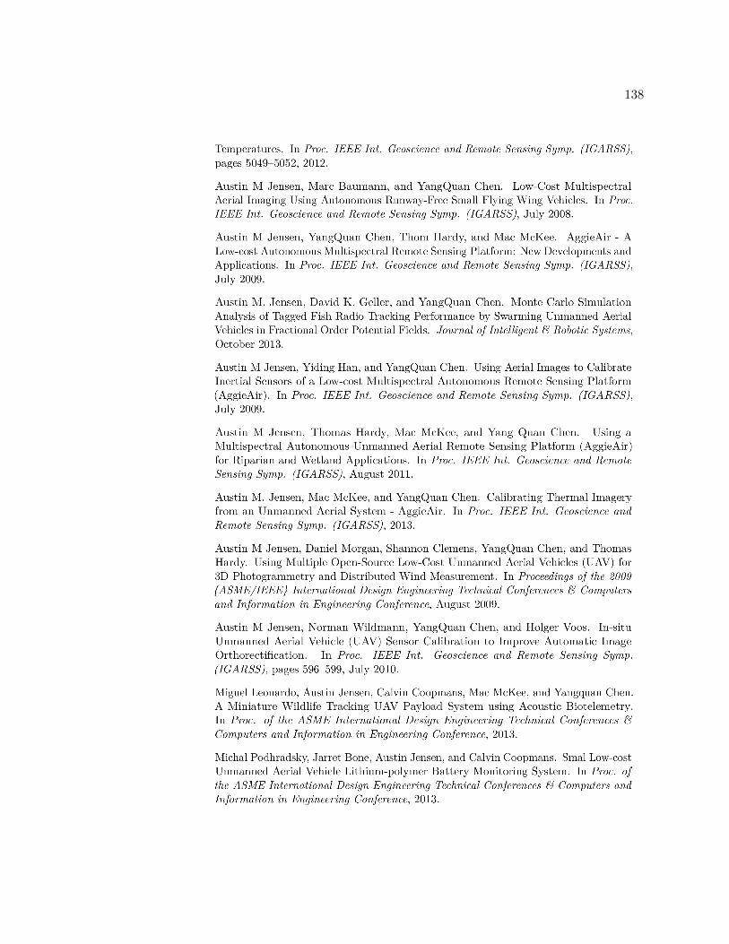
5.2.2 Monte Carlo Simulations
Table 5.2 shows the results of the Monte Carlo Simulations. The mean, the 3-sigma
values, and the 99% chi-squared confidence interval for the 3-sigma values are listed for all
four methods. Each method was also simulated with one, two and three UAs.
With a higher mean and 3-sigma value than any of the others, the Attractive method
seems to be the worst option. Focusing on the other three methods and the simulations
with just one UA, the following observations should be noted.
1. The two offset methods have very similar results and have a lower mean value than
the Repulsive Method.
2. The Repulsive Method may have a higher mean than the offset methods, but the
upper 3-sigma value is lower.
3. The Repulsive Method is the only one that has a lower 3-sigma value greater than
zero.
82
Table 5.2: Monte Carlo simulation results for tag error dispersion and 100 flights (meters).Method # of Final Upper Lower Chi-2
UAs Mean 3-sig 3-sig Spread
Att 1 274 671 0 149Rep 1 251 343 159 35
Offset 1 160 408 0 93Dual 1 160 360 0 76
Att 2 249 577 0 123Rep 2 256 325 187 27
Offset 2 168 411 0 98Dual 2 186 436 0 101
Att 3 234 572 0 127Rep 3 255 318 192 27
Offset 3 186 443 0 111Dual 3 190 471 0 108
4. The Repulsive has the smallest gap between the mean and the 3-sigma values and the
smallest Chi-2 spread.
The conclusion from these observations is that while the offset methods may achieve
higher accuracy estimates, they are less precise and have higher uncertainty. The Repulsive
Method may not be able to achieve errors as low as the Offset Methods, however is much
more reliable. The error trajectory plots of the Repulsive Method and the Offset Method
also confirm this conclusion (Figures 5.24 and 5.25)
The table also shows that with the Attractive and Repulsive methods, having multi-
ple UAs improved the estimation performance. The opposite is true with the Offset and
Dual-offset methods; they performed worse with more than one UA. Even so the general
improvement shown in the table from multiple UAs is not great. The greatest contribution
that multiple UAs made to the estimate is illustrated in the error trajectory plots. Figure
5.26 shows the trajectory plot for the Repulsive Method and three UAs. Compared to the
Repulsive plot with one UA (Figure 5.24), the plot with three UAs converges ten times
faster than the plot with one UA. Even though using multiple UAs did not improve the
error in the estimate, they can be used to find the tag in shorter time.
83
0 500 1000 1500 2000 2500 3000−400
−200
0
200
400
600
800
1000Tag Estimation Error Trajectories
Time (s)
Est
imat
ion
Err
or (
m)
Mean3 Sigma99% Chi2 Bounds
Number of Runs/Errors: 100/0Final Mean: 2513−Sig Values, Upper:343 Lower:159Chi−2 Spread: 34.6246
Fig. 5.24: MC simulation with 1 UA using Repulsive Method.
5.2.3 Summary
The simulation proved successful at implementing real-world disturbances like GPS
bias, a variable ground speed, and a crab angle. The estimation of the tag was also successful
despite the noisy signal and the simplified measurement model. The Monte Carlo analysis
showed that the Offset and Dual-offset Methods could estimate the tag with the highest
accuracy but also with the highest variability. The Repulsive Method was not able to
estimate with the same accuracy but was very consistent. The use of multiple UAs did not
improve the estimation accuracy; in some cases, it made the estimates worse. However,
multiple UAs were able to find the tag ten times faster than a single UA.
Future work includes sensitivity analysis to figure out which error sources are major
contributors to the tracking error. With this information, meaningful improvements can be
made on the platform to increase the accuracy. A well-tuned heading controller or wind
compensation could also increase the accuracy. Future work also includes looking at ways
to improve accuracy while using multiple UAs. This could possibly be achieved by keeping
the UAs in formation and by giving each its own unique antenna configuration.
84
0 500 1000 1500 2000 2500 3000−400
−200
0
200
400
600
800
1000Tag Estimation Error Trajectories
Time (s)
Est
imat
ion
Err
or (
m)
Mean3 Sigma99% Chi2 Bounds
Number of Runs/Errors: 100/0Final Mean: 1603−Sig Values, Upper:408 Lower:−88Chi−2 Spread: 93.3655
Fig. 5.25: MC simulation with 1 UA using Offset Repulsive Method.
5.3 Chapter Summary
This chapter illustrated how The Processing Cycle for Meaningful Remote Sensing
can be used in real-time to provide feedback to the end user and to improve the accuracy
of the actionable information. Simple, novel methods for radio-localization and multi-UA
navigation were presented and tested using a real-world simulation scenario. Monte Carlo
analysis was used to compare different navigation methods and to determine what expected
performance would be in real-world situations. Improvements could be made, either in the
payload or with the navigation methods, by doing a sensitivity analysis to find out which
error sources are major contributors to the tracking error.
85
0 500 1000 1500 2000 2500 3000−400
−200
0
200
400
600
800
1000Tag Estimation Error Trajectories
Time (s)
Est
imat
ion
Err
or (
m)
Mean3 Sigma99% Chi2 Bounds
Number of Runs/Errors: 100/20Final Mean: 2553−Sig Values, Upper:318 Lower:192Chi−2 Spread: 26.8739
Fig. 5.26: MC simulation with 3 UA using Repulsive Method.
86
Chapter 6
Delivering Actionable Information
Previous chapters have shown how imagery can be captured, georeferenced, and cali-
brated from small UAS with consumer-grade cameras. However, the Processing Cycle for
Meaningful Remote Sensing has not been completed. The last step, Application Processing,
converts the scientific data into actionable information which is used by the end user. If
this step is not done correctly and the data given to the end user is not useful, then there
is no point in gathering the data in the first place. This chapter shows a few examples of
how imagery from VIS-NIR and TIR cameras were used to provide actionable information
for applications in vegetation mapping, precision agriculture, and fish habitat.
6.1 Vegetation Mapping
One of the great uses for VIS-NIR imagery is vegetation mapping. The red, green,
blue, and NIR spectral bands of the VIS-NIR imagery contains a spectral fingerprint that
can be used to classify the imagery into different types of vegetation [38]. This tool is very
useful especially in managing problematic invasive plant species like Phragmites Australis.
Imported from Europe over a hundred years ago, this aggressive grass species is invading
wetlands across North America [63]. This causes many problems including displacing native
vegetation [64], loss of flora and fauna, alternations to wetland nutrient cycling, and loss
of habitat for many animals including birds [64–67]. At the Bear River Migratory Bird
Refuge (BRMBR) in northern Utah, Phragmites Australis creates an issue for migratory
birds on the Pacific Flyway which depend on this area as a resting stop [68]. To help control
Phragmites Australis wetland managers could really benefit from having maps which show
where it is, how it is growing, and which native plants are being replaced.
In 2010 and 2011, AggieAir was used to provide this information to wetland managers
87
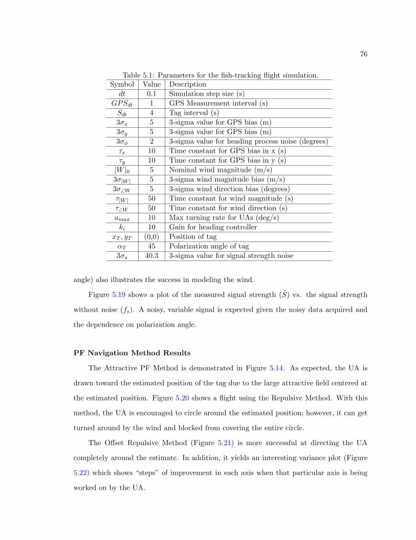
[68]. VIS-NIR images of a 12-square mile area were captured, orthorectified, and calibrated
using reflectance panels on four separate occasions over the summer. During the flight a
ground crew identified ground features including Phragmites australis, water, road, etc. and
surveyed the features using a survey grade GPS receiver. The calibrated VIS-NIR mosaics
and the ground samples were then used to train a multiclass relevance vector machine
(RVM) to classify the entire area. Figure 6.1 shows VIS-NIR mosaics with the resulting
classified image.
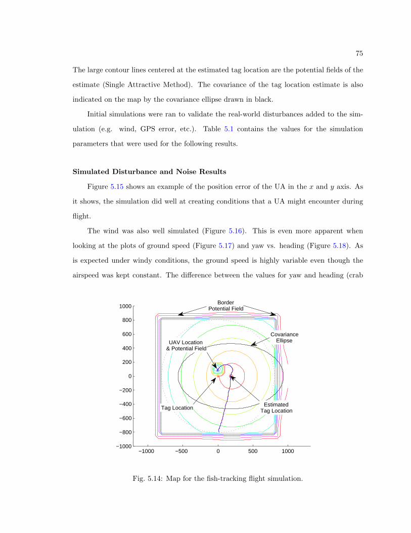
The classified image in Figure 6.1 is a form of actionable information which can be
used by wetland managers to help manage Phragmites australis. However since a series of
images were acquired, mosaiced, and classified, change detection was used to show growth
over the season (Figure 6.2). This additional actionable information can be used by the
wetland managers to plan for future removal administration.
Fig. 6.1: VIS-NIR mosaics and a classified image of Phragmites Australius.
88
Fig. 6.2: A series of vegetation maps can be used for change detection.
6.2 Precision Agriculture
Precision agriculture is a process of using large quantities of data in order to make
precise adjustments to agricultural inputs such as water and nutrients. Data from remote
sensing sources can be very valuable to precision agriculture [69–72], and remotely sensed
data from UAS can add even more value due to the high-resolution and flexible nature of
UAS. This was demonstrated in 2013 using AggieAir by flying over a small farm with two
center pivots five times over the course of two months [73, 74]. In addition to collecting
VIS-NIR imagery, TIR imagery was also collected for precision agriculture since it is very
important and includes data related to soil moisture and evaoptranspiration. This data
was converted into georeferenced scientific data using the techniques previously outlined
and used to generate maps with actionable information. Figure 6.3 shows the VIS-NIR and
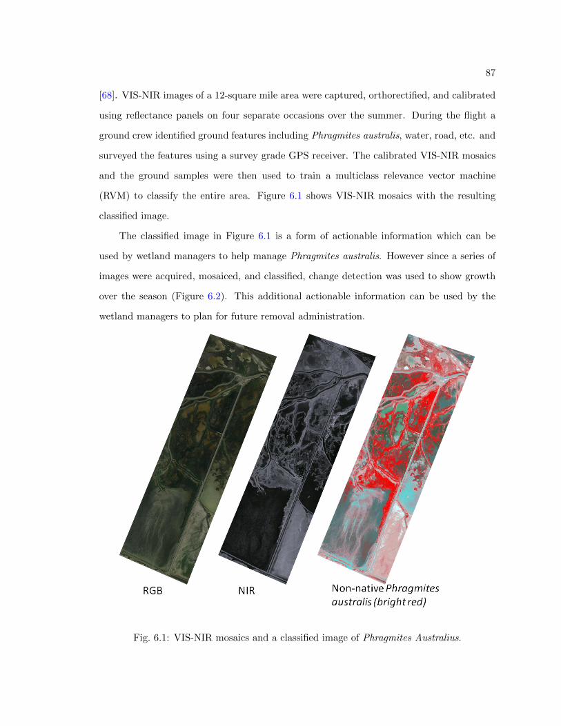
TIR mosaics of the area for one of the flights. To help generate the actionable information,
index maps such as the Normalized Difference Vegetation Index (NDVI) and Leaf Area
Index (LAI) are generated using the VIS-NIR mosaics (Figure 6.4). These maps are easy to
generate and do not represent anything physical; however they add additional sets of data
that are used when generating other maps.
89
Fig. 6.3: VIS-NIR and thermal mosaics of two center pivots.
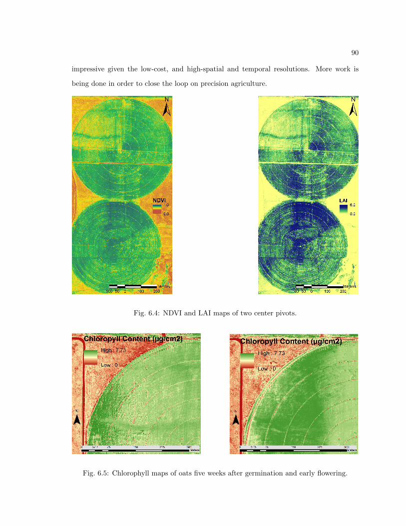
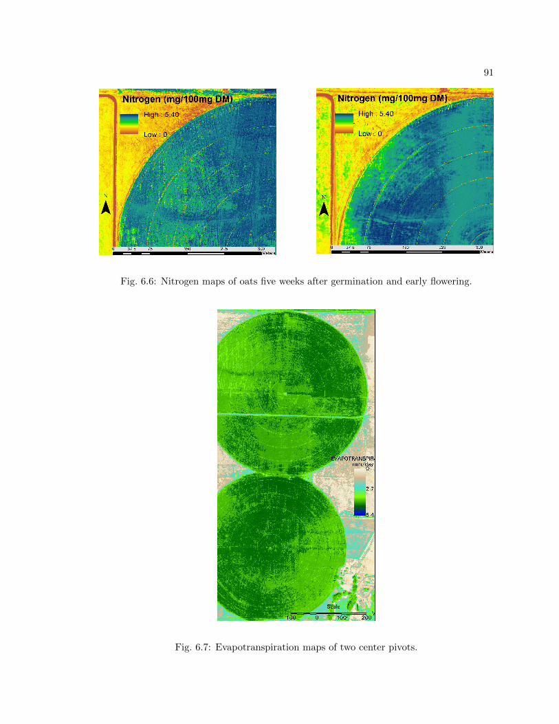
Figures 6.5, 6.6, and 6.7 show the results from the AggieAir fights. Figures 6.5 and 6.6
show the chlorophyll and nitrogen content of oats five weeks after germination and during
early flowering. Maps like these are used to quantify plant health and can be used for yield
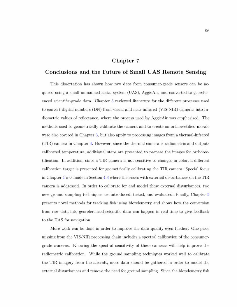
predictions and to tell the farmer where and how much fertilizer to apply. Figure 6.7 is
a map of evapotranspiration and describes how much water is being transpired from the
plant; the methods used to generate this map is widely used with satellite data [75] but has
shown good performance using the data from AggieAir. Similar methods can also be used
to estimate and forecast soil moisture which could be used when scheduling irrigation.
Many might call results like these sufficiently simplified for use in routine precision
agriculture. However further simplification is needed to reduce the data to fit the growers
form of actuation. If the grower uses a center pivot to irrigate, the data would need to be
presented in a way that the could be implemented on the pivot (e.g. when to turn it on
and how fast it should run). If the grower uses flood irrigation, the data might need to
be simplified even further to show which days to irrigate and which not to. Even though
the results presented in this section are arguably not yet actionable, they are still very
90
impressive given the low-cost, and high-spatial and temporal resolutions. More work is
being done in order to close the loop on precision agriculture.
Fig. 6.4: NDVI and LAI maps of two center pivots.
Fig. 6.5: Chlorophyll maps of oats five weeks after germination and early flowering.
91
Fig. 6.6: Nitrogen maps of oats five weeks after germination and early flowering.
Fig. 6.7: Evapotranspiration maps of two center pivots.
92
6.3 Fish Thermal Refugia
Temperature is a critical physical characteristic of aquatic systems due to its relation-
ship with chemical and biological reaction rates, and with aquatic species that are sensitive
to temperature. Attempts to quantify processes influencing temperature regimes commonly
include field based measurements at discrete locations that are often used to support in-
stream temperature modeling [76]. More recently, spatially representative observations from
distributed temperature sensing applications have been utilized in modeling efforts [77]. A
growing body of literature has illustrated the utility of high resolution remotely sensed TIR
imagery for mapping spatial temperature patterns in streams and rivers [15, 78] that pro-
vide information to identify biologically important areas such as thermal refugia [14] or to
understand the effects of land management practices on stream temperature [79]. The use
of thermal imagery to support temperature instream modeling has been shown to provide
important information regarding system behavior [80], however, the utility of these data
types in modeling is limited by the temporal, and at times the spatial resolution, of the
data.
To test the utility of AggieAir for the thermal refugia application, AggieAir was flown
over a river with significant ongoing research regarding changing temperature regimes within
the river. Visual, NIR, and thermal images were all acquired and stitched together into
separate orthorectified mosaics (Figure 6.8).
Since this application only requires stream temperature, it is necessary to separate the
stream from land in the thermal mosaic. The NIR mosaic is very effective in mapping
the banks of the river since water absorbs NIR light well. This makes water appear very
dark in the imagery and allows us to easily delineate between water and land. The visual
and thermal mosaics are also used to help map the banks of the river. After the stream
is digitized, it can be used to remove the land and vegetation from the thermal mosaics
(Figure 6.9). Removing the land is an important part of generating actionable information
because the data is more focused toward what is really needed by the end user. In addition
since the thermal mosaic only includes water, it can easily be corrected for emissivity and
93
Fig. 6.8: VIS-NIR and thermal mosaics of river.
calibrated using temperature probes within the river.
6.4 Cyber Physical System Based on small UAS-Based Remote Sensing
The Processing Cycle for Meaningful Remote Sensing is part of a larger Cyber Physical
System (CPS). A CPS is a system which includes hardware and software to provide sensing
and actuation to a large scale closed-loop system to manage high-level complex systems [81].
A good example of a CPS is precision agriculture. The UAS acts as a sensor and provides
actuators (automated center pivots, autonomous tractors) with data they can use to control
complex systems such as soil moisture or plant nitrogen content. The Processing Cycle for
Meaningful Remote Sensing is actually software that simply takes the data from the UAS
94
Fig. 6.9: Thermal mosaic of river displayed over visual mosaic.
and converts it in a form which can be understood by the actuators. Another example of
a CPS is using multiple UAs for diffusion control in diffusion processes such as chemical
and radiation leaks [82]. In this case, a group of sensor UAs could be used to measure the
diffusion process while another group of actuation or sprayer UAs could be used to release
chemicals to control the diffusion process.
6.5 Chapter Summary
This chapter showed some examples of how the Processing Cycle for Meaningful Remote
Sensing can be completed by proving actionable information to the users and how this
process is related to a CPS. For vegetation mapping, AggieAir VIS-NIR imagery was used
to map an invasive plant species to help wetland managers manage the species. In addition,
a series of images were captured over the growing season and change detection was used to
map how the invasive plant species was growing. In precision agriculture, AggieAir VIS-
NIR and TIR imagery was captured over two center pivots and used to generate maps of
95
plant chlorophyll, plant nitrogen, and evapotranspiration. While this data could be used
as actionable information to know where to apply nitrogen or where to water, more work
is still needed to simplify the data in a form that can be used by growers. Finally, an
application in mapping fish habitat was included. This showed how VIS-NIR imagery can
be used to map a river channel to simplify TIR imagery by removing the land so just the
surface temperature of the river is left: thereby giving biologists actionable information
about thermal refugia for fish.
96
Chapter 7
Conclusions and the Future of Small UAS Remote Sensing
This dissertation has shown how raw data from consumer-grade sensors can be ac-
quired using a small unmanned aerial system (UAS), AggieAir, and converted to georefer-
enced scientific-grade data. Chapter 3 reviewed literature for the different processes used
to convert digital numbers (DN) from visual and near-infrared (VIS-NIR) cameras into ra-
diometric values of reflectance, where the process used by AggieAir was emphasized. The
methods used to geometrically calibrate the camera and to create an orthorectified mosaic
were also covered in Chapter 3, but also apply to processing images from a thermal-infrared
(TIR) camera in Chapter 4. However, since the thermal camera is radiometric and outputs
calibrated temperature, additional steps are presented to prepare the images for orthorec-
tification. In addition, since a TIR camera is not sensitive to changes in color, a different
calibration target is presented for geometrically calibrating the TIR camera. Special focus
in Chapter 4 was made in Section 4.3 where the issues with external disturbances on the TIR
camera is addressed. In order to calibrate for and model these external disturbances, two
new ground sampling techniques are introduced, tested, and evaluated. Finally, Chapter 5
presents novel methods for tracking fish using biotelemetry and shows how the conversion
from raw data into georeferenced scientific data can happen in real-time to give feedback
to the UAS for navigation.
More work can be done in order to improve the data quality even further. One piece
missing from the VIS-NIR processing chain includes a spectral calibration of the consumer-
grade cameras. Knowing the spectral sensitivity of these cameras will help improve the
radiometric calibration. While the ground sampling techniques worked well to calibrate
the TIR imagery from the aircraft, more data should be gathered in order to model the
external disturbances and remove the need for ground sampling. Since the biotelemetry fish
97
tracking application is still in its infancy, lots of work is needed to be done before this is
made for routine use. Additional simulations are needed to perform sensitivity analysis and
find out ways to improve the accuracy of the tag location estimation. At that point, the
navigation routines need to be implemented in the autopilot and real-world experiments
should be conducted under different scenarios to prove the system.
There is a lot of potential for using small UAS as a remote sensing platform. They
have proved very useful in delivering quality data for many applications including vegetation
mapping, fish habitat mapping, and precision agriculture. Perhaps if The Processing Cycle
for Remote Sensing becomes more automated and actionable information can be delivered
at the click of a button, small UAS will enable remote sensing to become “personal.” And
like personal computers or phones, many will be able to use small UAS to improve their
everyday lives.
98
References
[1] R. Benedetti and P. Rossini, “On the use of NDVI Profiles as a Tool for AgriculturalStatistics: The Case Study of Wheat Yield Estimate and Forecast in Emilia Romagna,”Remote Sensing of Environment, vol. 45, no. 3, pp. 311–326, Sept. 1993.
[2] B. Rudorff and G. Batista, “Yield Estimation of Sugarcane Based onAgrometeorological-Spectral Models,” Remote Sensing of Environment, vol. 33, no. 3,pp. 183–192, Sept. 1990.
[3] M. L. Stone, J. B. Solie, W. R. Raun, R. W. Whitney, S. L. Taylor, and J. D. Ringer,“Use of Spectral Radiance for Correcting in-season Fertilizer Nitrogen Deficiencies inWinter Wheat,” Transactions of the American Society of Agricultural and BiologicalEngineers, vol. 39, no. 5, pp. 1623–1631, 1996.
[4] R. D. Jackson, S. B. Idso, R. J. Reginato, and P. J. Pinter, “Canopy Temperature as aCrop Water Stress Indicator,” Water Resources Research, vol. 17, no. 4, p. 1133, 1981.
[5] A. Mathur and G. M. Foody, “Crop Classification by Support Vector Machine withIntelligently Selected Training Data for an Operational Application,” InternationalJournal of Remote Sensing, vol. 29, no. 8, pp. 2227–2240, Apr. 2008.
[6] J. Franke and G. Menz, “Multi-temporal Wheat Disease Detection by Multi-spectralRemote Sensing,” Precision Agriculture, vol. 8, no. 3, pp. 161–172, June 2007.
[7] S. Thomson, L. Smith, J. Ray, and P. Zimba, “Remote Sensing and Implications forVariable-rate Application Using Agricultural Aircraft,” in Proceedings of Society ofPhotographic Instrumentation Engineers, vol. 5153, 2004, p. 13.
[8] N. Coops and P. Catling, “Predicting the Complexity of Habitat in Forests from Air-borne Videography for Wildlife Management,” International Journal of Remote Sens-ing, vol. 18, no. 12, 1997.
[9] R. D. Wulf and R. Goossens, “Remote Sensing for Wildlife Management: Giant PandaHabitat Mapping from LANDSAT MSS Images,” Geocarto International, vol. 3, no. 1,1988.
[10] J. H. Everitt, C. Yang, R. S. Fletcher, C. J. Deloach, and M. R. Davis, “Using RemoteSensing to Assess Biological Control of Saltcedar,” Southwestern Entomologist, vol. 32,no. 2, pp. 93–103, June 2007.
[11] P. H. Evangelista, T. J. Stohlgren, J. T. Morisette, and S. Kumar, “Mapping Inva-sive Tamarisk (Tamarix): A Comparison of Single-scene and Time-series Analyses ofRemotely Sensed Data,” Remote Sensing, vol. 1, no. 3, pp. 519–533, Aug. 2009.
[12] S. Sriharan, J. Everitt, C. Yang, and R. Fletcher, “Mapping Riparian and WetlandWeeds with High Resolution Satellite Imagery,” in Proceedings IEEE InternationalGeoscience and Remote Sensing Symposium (IGARSS), 2008.
99
[13] C. Walter and D. D. Tullos, “Downstream Channel Changes after a Small Dam Re-moval: Using Aerial Photos and Measurement Error for Context; Calapooia River,Oregon,” River Research and Applications, vol. 26, no. 10, pp. 1220–1245, Dec. 2010.
[14] C. E. Torgersen, D. M. Price, H. W. Li, and B. A. McIntosh, “Multiscale ThermalRefugia and Stream Habitat Associations of Chinook Salmon in Northeastern Oregon,”Ecological Applications, vol. 9, no. 1, pp. 301–319, Feb. 1999.
[15] J. Kay, R. Handcock, A. Gillespie, C. Konrad, S. Burges, N. Naveh, and D. Booth,“Stream-temperature Estimation from Thermal Infrared Images,” in IEEE 2001 Inter-national Geoscience and Remote Sensing Symposium, vol. 1. IEEE, 2001, pp. 112–114.
[16] P. Coppin and M. Bauer, “Digital Change Detection in Forest Ecosystems with RemoteSensing Imagery,” Remote Sensing Reviews, vol. 13, no. 3-4, 1996.
[17] M. Lefsky, D. Harding, and W. Cohen, “Surface Lidar Remote Sensing of Basal Areaand Biomass in Deciduous Forests of Eastern Maryland, USA,” Remote Sensing ofEnvironment, vol. 67, no. 1, pp. 83–98, 1999.
[18] C. Wessman, J. Aber, D. Peterson, and J. Melillo, “Remote Sensing of Canopy Chem-istry and Nitrogen Cycling in Temperate Forest Ecosystems,” Nature, vol. 335, no.6186, 1988.
[19] S. G. Bajwa and E. D. Vories, “Spectral Response of Cotton Canopy to Water Stress,”in Proceedings of the American Society of Agricultural and Biological Engineers AnnualMeeting, July 2006.
[20] R. H. Gray and J. M. Haynes, “Spawning Migration of Adult Chinook Salmon ( On-corhynchus tshawytscha ) Carrying External and Internal Radio Transmitters,” Journalof the Fisheries Research Board of Canada, vol. 36, no. 9, pp. 1060–1064, Sept. 1979.
[21] A. Rango, A. Laliberte, J. E. Herrick, C. Winters, K. Havstad, C. Steele, and D. Brown-ing, “Unmanned Aerial Vehicle-based Remote Sensing for Rangeland Assessment, Mon-itoring, and Management,” Journal of Applied Remote Sensing, vol. 3, no. 1, p. 033542,Jan. 2009.
[22] J. Berni, P. J. Zarco-Tejada, L. Suarez, and E. Fereres, “Thermal and NarrowbandMultispectral Remote Sensing for Vegetation Monitoring from an Unmanned AerialVehicle,” IEEE Transactions on Geoscience and Remote Sensing, vol. 47, no. 3, pp.722–738, Mar. 2009.
[23] L. Wallace, A. Lucieer, C. Watson, and D. Turner, “Development of a UAV-LiDARSystem with Application to Forest Inventory,” Remote Sensing, vol. 4, no. 6, pp. 1519–1543, May 2012.
[24] A. M. Jensen, T. Hardy, M. McKee, and Y. Q. Chen, “Using a Multispectral Au-tonomous Unmanned Aerial Remote Sensing Platform (AggieAir) for Riparian andWetland Applications,” in Proceedings IEEE International Geoscience and RemoteSensing Symposium (IGARSS), Aug. 2011.
100
[25] A. Laliberte, C. Winters, and A. Rango, “UAS Remote Sensing Missions for RangelandApplications,” Geocarto International, vol. 26, no. 2, pp. 141–156, Dec. 2011.
[26] A. M. Jensen, M. McKee, and Y. Chen, “Calibrating Thermal Imagery from an Un-manned Aerial System - AggieAir,” in Proceedings IEEE International Geoscience andRemote Sensing Symposium (IGARSS), 2013.
[27] A. M. Jensen, D. K. Geller, and Y. Chen, “Monte Carlo Simulation Analysis of TaggedFish Radio Tracking Performance by Swarming Unmanned Aerial Vehicles in FractionalOrder Potential Fields,” Journal of Intelligent & Robotic Systems, vol. 74, no. 1-2, pp.287–307, Oct. 2014.
[28] “Academy of Model Aeronautics Membership Manual,” Academy of Model Aeronau-tics, 2014. [Online]. Available: https://www.modelaircraft.org/files/memanual.pdf
[30] A. S. Laliberte, M. A. Goforth, C. M. Steele, and A. Rango, “Multispectral RemoteSensing from Unmanned Aircraft: Image Processing Workflows and Applications forRangeland Environments,” Remote Sensing, vol. 3, no. 11, pp. 2529–2551, Nov. 2011.
[31] J. Kelcey and A. Lucieer, “Sensor Correction of a 6-Band Multispectral Imaging Sensorfor UAV Remote Sensing,” Remote Sensing, vol. 4, no. 5, pp. 1462–1493, May 2012.
[32] J. Berni, P. J. Zarco-Tejada, L. Surez, V. Gonzalez-Dugo, and E. Fereres, “RemoteSensing of Vegetation from UAV Platforms using Lightweight Multispectral and Ther-mal Imaging Sensors,” in The International Archives of the Photogrammetry, RemoteSensing and Spatial Information Sciences, 2008.
[33] A. Simpson, T. Stombaugh, L. Wells, and J. Jacob, “Imaging Techniques and Applica-tions for UAV’s in Agriculture,” in Proceedings of the American Society of Agriculturaland Biological Engineers Annual Meeting, July 2003.
[34] C. Coopmans, B. Stark, and C. M. Coffin, “A Payload Verification and ManagementFramework for Small UAV-based Personal Remote Sensing Systems,” in Proceedingsof the 5th International Symposium on Resilient Control Systems. IEEE, Aug. 2012,pp. 184–189.
[35] G. L. Ritchie, D. G. Sullivan, C. D. Perry, J. E. Hook, and C. W. Bednarz, “Preparationof a Low-Cost Digital Camera System for Remote Sensing,” Applied Engineering inAgriculture, vol. 24, no. 6, pp. 885–894, 2008.
[36] T. Miura and A. Huete, “Performance of Three Reflectance Calibration Methods forAirborne Hyperspectral Spectrometer Data,” Sensors, vol. 9, no. 2, pp. 794–813, 2009.
[37] E. R. Hunt, M. Cavigelli, C. S. T. Daughtry, J. E. Mcmurtrey, and C. L. Walthall,“Evaluation of Digital Photography from Model Aircraft for Remote Sensing of CropBiomass and Nitrogen Status,” Precision Agriculture, vol. 6, no. 4, pp. 359–378, Aug.2005.
[38] S. Clemens, “Procedures for Correcting Digital Camera Imagery Acquired by the Ag-gieAir Remote Sensing Platform,” Master’s thesis, Utah State University, 2012.
[39] J. Kannala, J. Heikkila, and S. S. Brandt, “Geometric Camera Calibration,” in WileyEncyclopedia of Computer Science and Engineering. Hoboken, NJ: John Wiley &Sons, Inc., Mar. 2007, pp. 1–11.
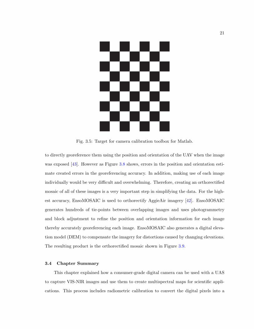
[40] J. Bouguet, “Camera Calibration Toolbox for Matlab,” 2012. [Online]. Available:http://www.vision.caltech.edu/bouguetj/calib doc/
[41] J. Heikkila and O. Silven, “A Four-Step Camera Calibration Procedure with ImplicitImage Correction,” in Proceedings of IEEE Computer Society Conference on ComputerVision and Pattern Recognition. IEEE Computer Society, 1997, pp. 1106–1112.
[43] A. Jensen, “gRAID: A Geospatial Real-Time Aerial Image Display for a Low-Cost Au-tonomous Multispectral Remote Sensing Platform (AggieAir),” Master’s thesis, UtahState University, 2009.
[44] W. Ji and P. Rhodes, “Spectral Color Characterization of Digital Cameras: A Review,”in Proceedings of Society of Photographic Instrumentation Engineers Vol, 2012.
[45] C. E. Torgersen, R. N. Faux, B. A. McIntosh, N. J. Poage, and D. J. Norton, “AirborneThermal Remote Sensing for Water Temperature Assessment in Rivers and Streams,”Remote Sensing of Environment, vol. 76, no. 3, pp. 386–398, 2001.
[46] M. A. Gallo, D. S. Willits, R. A. Lubke, and E. C. Thiede, “Low-cost Uncooled IRSensor for Battlefield Surveillance,” in Proceedings Society of Photographic Instrumen-tation Engineers 2020, Infrared Technology XIX, vol. 2020, 1993, pp. 351–362.
[47] T. W. Parker, C. A. Marshall, M. Kohin, and R. Murphy, “Uncooled Infrared Sensorsfor Surveillance and Law Enforcement Applications,” in Proceedings Society of Pho-tographic Instrumentation Engineers 2935, Surveillance and Assessment Technologiesfor Law Enforcement, vol. 2935, 1997, pp. 182–187.
[49] A. Jensen, B. Neilson, M. McKee, and Y. Chen, “Thermal Remote Sensing With anAutonomous Unmanned Aerial Remote Sensing Platform for Surface Stream Tempera-tures,” in Proceedings IEEE International Geoscience and Remote Sensing Symposium(IGARSS), 2012, pp. 5049–5052.
[50] A. J. Prata, “Land Surface Temperatures Derived from the Advanced Very High Res-olution Radiometer and the Along-Track Scanning Radiometer: 2. Experimental Re-sults and Validation of AVHRR Algorithms,” Journal of Geophysical Research, vol. 99,no. D6, 1994.
[51] G. Wukelic, D. Gibbons, L. Martucci, and H. Foote, “Radiometric Calibration of Land-sat Thematic Mapper Thermal Band,” Remote Sensing of Environment, vol. 28, pp.339–347, 1989.
[52] R. R. Irish, “Landsat 7 Science Data Users Handbook,” National Aeronautics andSpace Administration, 2000.
[53] “Landsat Data Continuity Mission,” 2013. [Online]. Available: http://ldcm.gsfc.nasa.gov/index.html
[54] R. W. Hillyard and E. R. Keeley, “Distribution and Spawning Migrations of FluvialBonneville Cutthroat Trout in the Bear River, Idaho,” Idaho State University, Feb.,2009.
[55] M. Leonardo, A. Jensen, C. Coopmans, M. McKee, and Y. Chen, “A Miniature WildlifeTracking UAV Payload System using Acoustic Biotelemetry,” in Proceedings of theASME International Design Engineering Technical Conferences & Computers and In-formation in Engineering Conference, Portland, Aug. 2013.
[56] E. W. Frew, C. Dixon, B. Argrow, and T. Brown, “Radio Source Localization by aCooperating UAV Team,” in Infotech@ Aerospace, 2005.
[57] F. Korner, R. Speck, A. H. Goktogan, and S. Sukkarieh, “Autonomous AirborneWildlife Tracking Using Radio Signal Strength,” in Proceedings of the IEEE/RSJ In-ternational Conference on Intelligent Robots and Systems. IEEE, Oct. 2010, pp.107–112.
[58] S. Ge and Y. Cui, “Dynamic Motion Planning for Mobile Robots Using Potential FieldMethod,” Autonomous Robots, vol. 13, no. 3, pp. 207–222, Nov. 2002.
[59] T. Paul, T. R. Krogstad, and J. T. Gravdahl, “Modelling of UAV Formation FlightUsing 3D Potential Field,” Simulation Modelling Practice and Theory, vol. 16, no. 9,pp. 1453–1462, Oct. 2008.
[60] O. Khatib, “Real-time Obstacle Avoidance for Manipulators and Mobile Robots,” inProceedings of the IEEE International Conference on Robotics and Automation, vol. 2.Institute of Electrical and Electronics Engineers, 1985, pp. 500–505.
[61] Y. Chen, Z. Wang, and K. Moore, “Optimal Spraying Control of a Diffusion ProcessUsing Mobile Actuator Networks with Fractional Potential Field Based Dynamic Ob-stacle Avoidance,” in Proceedings of the IEEE International Conference on Networking,Sensing and Control. IEEE, 2006, pp. 107–112.
[62] K. Miller, “The Weyl Fractional Calculus,” in Fractional Calculus and Its Applications,ser. Lecture Notes in Mathematics, B. Ross, Ed. Berlin, Heidelberg: Springer, 1975,vol. 457, pp. 80–89.
[63] S. Galatowitsch, N. Anderson, and P. Ascher, “Invasiveness in Wetland Plants in Tem-perate North America,” Wetlands, vol. 19, no. 4, pp. 733–755, 1999.
[64] M. Marks, B. Lapin, and J. Randall, “Phragmites Australis (P. communis): Threats,Management and Monitoring.” Natural Areas Journal, 1994.
[65] L. Meyerson, R. Chambers, and K. Vogt, “The Effects of Phragmites Removal onNutrient Pools in a Freshwater Tidal Marsh Ecosystem,” Biological Invasions, vol. 1,no. 2-3, pp. 129–136, 1999.
[66] L. Meyerson, K. Saltonstall, and L. Windham, “A Comparison of Phragmites Australisin Freshwater and Brackish Marsh Environments in North America,” Wetlands Ecologyand Management, vol. 8, no. 2-3, pp. 89–103, 2000.
[67] L. Windham and J. Ehrenfeld, “Net Impact of a Plant Invasion on Nitrogen-cyclingProcesses within a Brackish Tidal Marsh,” Ecological Applications, vol. 13, pp. 883–896, 2003.
[68] B. Zaman, M. McKee, and A. Jensen, “Use of High-Resolution Multispectral ImageryAcquired with an Autonomous Unmanned Aerial Vehicle to Quantify the Spread of anInvasive Wetland Species,” in Proceedings IEEE International Geoscience and RemoteSensing Symposium (IGARSS), Aug. 2011.
[69] M. Moran, Y. Inoue, and E. Barnes, “Opportunities and Limitations for Image-basedRemote Sensing in Precision Crop Management,” Remote Sensing of Environment,vol. 61, no. 3, pp. 319–346, 1997.
[70] B. Brisco, R. Brown, and T. Hirose, “Precision Agriculture and the Role of RemoteSensing: A Review,” Can J Remote Sensing, vol. 24, no. 3, pp. 315–327, 1998.
[71] R. Pearson, J. Grace, and G. May, “Real-time Airborne Agricultural Monitoring,”Remote Sensing of Environment, vol. 49, no. 3, pp. 304–310, 1994.
[72] D. Lamb and R. Brown, “Precision Agriculture: Remote-Sensing and Mapping ofWeeds in Crops,” Journal of Agricultural Engineering Research, vol. 78, no. 2, pp.117–125, 2001.
[73] M. Al-Arab, A. M. Ticlavilca, A. F. Torres-Rua, I. Maslova, and M. McKee, “Use ofHigh-Resolution Multispectral Imagery to Estimate Chrorophyll and Plant Nitrogen inOats (Avena sativa),” Abstract B43C-0493 presented at 2013 Fall Meeting, AmericanGeophysical Union (AGU), San Francisco, CA, 2013.
[74] M. Al-Arab, A. Torres-Rua, A. Ticlavilca, A. Jensen, and M. McKee, “Use of High-Resolution Multispectral Imagery from an Unmanned Aerial Vehicle in Precision Agri-culture,” in Proceedings IEEE International Geoscience and Remote Sensing Sympo-sium (IGARSS), 2013.
[75] A. F. Torres-Rua, W. R. Walker, and M. McKee, “The Lower Sevier River BasinCrop Monitor and Forecast Decision Support System: Exploiting Landsat Imagery toProvide Continuous Information to Farmers and Water Managers,” Abstract IN14A-07presented at 2013 Fall Meeting, American Geophysical Union (AGU), San Francisco,CA, 2013.
104
[76] G. W. Brown, “Predicting Temperatures of Small Streams,” Water Resources Research,vol. 5, no. 1, p. 68, 1969.
[77] M. C. Westhoff, H. H. G. Savenije, W. M. J. . Luxemburg, G. S. Stelling, N. C. Van DeGiesen, J. S. Selker, L. Pfister, and S. Uhlenbrook, “A Distributed Stream TemperatureModel using High Resolution Temperature Observations,” Hydrology and Earth SystemSciences, vol. 11, no. 4, pp. 1469–1480, July 2007.
[78] B. H. Atwell, R. B. MacDonald, and L. A. Bartolucci, “Thermal Mapping of Streamsfrom Airborne Radiometric Scanning,” Journal of the American Water Resources As-sociation, vol. 7, no. 2, pp. 228–243, Apr. 1971.
[79] D. J. Norton, M. A. Flood, B. McIntosh, N. J. Poage, P. J. LaPlaca, J. P. Craig, S. R.Karalus, J. R. Sedell, C. Torgersen, Y. D. Chen, S. C. McCutheeon, S. C. Duong,H. Puffenberger, J. Moeller, V. Kelley, E. Porter, and L. Shoemaker, “Modeling, Mon-itoring, and Restoring Water Quality and Habitat in the Pacific Northwestern Water-sheds,” U.S. Environmental Protection Agency, Washington, DC, 1996.
[80] N. C. Cristea and S. J. Burges, “Use of Thermal Infrared Imagery to ComplementMonitoring and Modeling of Spatial Stream Temperatures,” Journal of HydrologicEngineering, vol. 14, no. 10, p. 1080, Feb. 2009.
[81] C. Coopmans, B. Stark, A. Jensen, Y. Chen, and M. McKee, “Cyber-Physical Sys-tems Enabled By Small Unmanned Aerial Vehicles,” in Handbook of Unmanned AerialVehicles, K. P. Valavanis and G. J. Vachtsevanos, Eds. New York, NY: Springer, 2014.
[82] H. Chao and Y. Chen, Remote Sensing and Actuation Using Unmanned Vehicles.Hoboken, NJ: Wiley-IEEE Press, 2012.
105
Appendix
106
Certificate of Authorization
This appendix contains an FAA COA given to Utah State University using AggieAir
to fly on the North slope of Alaska near a remote field station called Toolik. The flight op-
erations for this COA and part of the pre-flight checklist for airworthiness are also included.
FAA FORM 7711-1 UAS COA Attachment 2013-WSA-63
Version 2.1: June 2012
Page 1 of 22
DEPARTMENT OF TRANSPORTATION FEDERAL AVIATION ADMINISTRATION
CERTIFICATE OF WAIVER OR AUTHORIZATION
ISSUED TO
Utah Water Research Laboratory - Utah State University 8200 Old Main Hill Logan, UT 84322 This certificate is issued for the operations specifically described hereinafter. No person shall conduct any operation pursuant to the authority of this certificate except in accordance with the standard and special provisions contained in this certificate, and such other requirements of the Federal Aviation Regulations not specifically waived by this certificate. OPERATIONS AUTHORIZED Operation of the AggieAir Unmanned Aircraft System (UAS) in Class G airspace at or below 1,000 feet Above Ground Level (AGL) in the vicinity of the Kuparuk River basin (as depicted in Attachment 1) under the jurisdiction of Anchorage Air Route Traffic Control Center (ARTCC). LIST OF WAIVED REGULATIONS BY SECTION AND TITLE
N/A
STANDARD PROVISIONS 1. A copy of the application made for this certificate shall be attached and become a part hereof. 2. This certificate shall be presented for inspection upon the request of any authorized representative of the Federal Aviation Administration, or of any State or municipal official charged with the duty of enforcing local laws or regulations. 3. The holder of this certificate shall be responsible for the strict observance of the terms and provisions contained herein. 4. This certificate is nontransferable. Note-This certificate constitutes a waiver of those Federal rules or regulations specifically referred to above. It does not constitute a waiver of any State law or local ordinance.
SPECIAL PROVISIONS
Special Provisions are set forth and attached.
This certificate 2013-WSA-63 is effective from June 25, 2013 to June 24, 2015, and is subject to cancellation at any time upon notice by the Administrator or his/her authorized representative.
BY DIRECTION OF THE ADMINISTRATOR
FAA Headquarters, AJV-115 Douglas Gould (Region) (Signature)
June 21, 2013 Air Traffic Manager, UAS Tactical Operations Section (Date) (Title)
FAA Form 7711-1 (7-74)
FAA FORM 7711-1 UAS COA Attachment 2013-WSA-63
Version 2.1: June 2012
Page 2 of 22
COA Number: 2013-WSA-63 Issued To: Utah Water Research Laboratory - Utah State University, referred herein as the “proponent” Address: 8200 Old Main Hill Logan, UT 84322 Activity: Operation of the AggieAir Unmanned Aircraft System (UAS) in Class G airspace at or below 1,000 feet Above Ground Level (AGL) in the vicinity of the Kuparuk River basin (as depicted in Attachment 1) under the jurisdiction of Anchorage Air Route Traffic Control Center (ARTCC). Purpose: To prescribe UAS operating requirements in the National Airspace System (NAS) for the purpose of quantifying the influences of lateral inflows on river water temperatures in the Kuparuk River basin. Dates of Use: This COA is valid from June 25, 2013 to June 24, 2015. Should a renewal become necessary, the proponent shall advise the Federal Aviation Administration (FAA), in writing, no later than 45 business days prior to the requested effective date. Public Aircraft
1. A public aircraft operation is determined by statute, 49 USC §40102(a)(41) and §40125.
2. All public aircraft flights conducted under a COA must comply with the terms of the statute.
3. All flights must be conducted per the declarations submitted on COA on-line.
FAA FORM 7711-1 UAS COA Attachment 2013-WSA-63
Version 2.1: June 2012
Page 3 of 22
STANDARD PROVISIONS A. General.
The review of this activity is based upon current understanding of UAS operations and their impact in the NAS. This COA will not be considered a precedent for future operations. (As changes in or understanding of the UAS industry occur, limitations and conditions for operations will be adjusted.)
All personnel connected with the UAS operation must read and comply with the contents of this authorization and its provisions.
A copy of the COA including the special limitations must be immediately available to all operational personnel at each operating location whenever UAS operations are being conducted.
This authorization may be canceled at any time by the Administrator, the person authorized to grant the authorization, or the representative designated to monitor a specific operation. As a general rule, this authorization may be canceled when it is no longer required, there is an abuse of its provisions, or when unforeseen safety factors develop. Failure to comply with the authorization is cause for cancellation. The proponent will receive written notice of cancellation.
During the time this COA is approved and active, a site safety evaluation/visit may be accomplished to ensure COA compliance, assess any adverse impact on ATC or airspace, and ensure this COA is not burdensome or ineffective. Deviations, accidents/incidents/mishaps, complaints, etc will prompt a COA review or site visit to address the issue. Refusal to allow a site safety evaluation/visit may result in cancellation of the COA. Note: This section does not pertain to agencies that have other existing agreements in place with the FAA.
B. Airworthiness Certification.
The unmanned aircraft must be shown to be airworthy to conduct flight operations in the NAS. Utah Water Research Laboratory - Utah State University has made its own determination that the AggieAir unmanned aircraft is airworthy. The AggieAir must be operated in strict compliance with all provisions and conditions contained in the Airworthiness Safety Release, including all documents and provisions referenced in the COA application.
1. A configuration control program must be in place for hardware and/or software changes
made to the UAS to ensure continued airworthiness. If a new or revised Airworthiness Release is generated as a result of changes in the hardware or software affecting the operating characteristics of the UAS, notify the UAS Integration Office of the changes as soon as practical.
FAA FORM 7711-1 UAS COA Attachment 2013-WSA-63
Version 2.1: June 2012
Page 4 of 22
a. Software and hardware changes should be documented as part of the normal maintenance procedures. Software changes to the aircraft and control station as well as hardware system changes are classified as major changes unless the agency has a formal process, accepted by the FAA. These changes should be provided to the UAS Integration office in summary form at the time of incorporation.
b. Major modifications or changes, performed under the COA, or other
authorizations that could potentially affect the safe operation of the system must be documented and provided to the FAA in the form of a new AWR, unless the agency has a formal process, accepted by the FAA.
c. All previously flight proven systems to include payloads, may be installed or
removed as required, and that activity recorded in the unmanned aircraft and ground control stations logbooks by persons authorized to conduct UAS maintenance Describe any payload equipment configurations in the UAS logbook that will result in a weight and balance change, electrical loads, and or flight dynamics, unless the agency has a formal process, accepted by the FAA.
d. For unmanned aircraft system discrepancies, a record entry should be made by an
appropriately rated person to document the finding in the logbook. No flights may be conducted following major changes, modifications or new installations unless the party responsible for certifying airworthiness has determined the system is safe to operate in the NAS and a new AWR is generated, unless the agency has a formal process, accepted by the FAA. The successful completion of these tests must be recorded in the appropriate logbook, unless the agency has a formal process, accepted by the FAA.
2. The AggieAir must be operated in strict compliance with all provisions and conditions contained within the spectrum analysis assigned and authorized for use within the defined operations area.
3. All items contained in the application for equipment frequency allocation must be
adhered to, including the assigned frequencies and antenna equipment characteristics. A ground operational check to verify the control station can communicate with the aircraft (frequency integration check) must be conducted prior to the launch of the unmanned aircraft to ensure any electromagnetic interference does not adversely affect control of the aircraft.
4. The use of a Traffic Collision Avoidance System (TCAS) in any mode while operating an
unmanned aircraft is prohibited. C. Operations.
1. Unless otherwise authorized as a special provision, a maximum of one unmanned aircraft will be controlled:
FAA FORM 7711-1 UAS COA Attachment 2013-WSA-63
Version 2.1: June 2012
Page 5 of 22
a. In any defined operating area,
b. From a single control station, and
c. By one pilot at a time.
2. A Pilot-in-Command (PIC) is the person who has final authority and responsibility for the operation and safety of flight, has been designated as PIC before or during the flight, and holds the appropriate category, class, and type rating, if appropriate, for the conduct of the flight. The responsibility and authority of the PIC as described by 14 CFR 91.3, Responsibility and Authority of the Pilot-in-Command, apply to the unmanned aircraft PIC. The PIC position may rotate duties as necessary with equally qualified pilots. The individual designated as PIC may change during flight. Note: The PIC can only be the PIC for one aircraft at a time. For Optionally Piloted Aircraft (OPA), PIC must meet UAS guidance requirements for training, pilot licensing, and medical requirements when operating OPA as a UAS.
3. The PIC must conduct a pre-takeoff briefing as applicable prior to each launch. The
briefing should include but is not limited to the:
a. Contents of the COA,
b. Altitudes to be flown,
c. Mission overview including handoff procedures,
d. Frequencies to be used,
e. Flight time, including reserve fuel requirements,
f. Contingency procedures to include lost link, divert, and flight termination, and
g. Hazards unique to the flight being flown.
Note: Flight Crew Member (UAS). In addition to the flight crew members identified in 14 CFR Part 1, Definitions and Abbreviations, an Unmanned Aircraft System flight crew members include pilots, sensor/payload operators, and visual observers and may include other persons as appropriate or required to ensure safe operation of the aircraft.
4. All operations will be conducted in compliance with Title 14 CFR Part 91. Special attention should be given to:
a. § 91.3 Responsibility and authority of the pilot in command
b. § 91.13 Careless or reckless operation
c. § 91.17 Alcohol or drugs
d. § 91.103 Preflight Actions
e. § 91.111 Operating near other aircraft.
f. § 91.113 Right-of-way rules: Except water operations
g. § 91.115 Right-of-way rules: Water operations
FAA FORM 7711-1 UAS COA Attachment 2013-WSA-63
Version 2.1: June 2012
Page 6 of 22
h. § 91.119 Minimum safe altitudes: General
i. § 91.123 Compliance with ATC clearances and instructions.
j. § 91.133 Restricted and prohibited areas
k. § 91.137 Temporary flight restrictions in the vicinity of disaster/hazard areas
l. § 91.145 Management of aircraft operations in the vicinity of aerial demonstrations and major sporting events
m. § 91.151 Fuel requirements for flight in VFR conditions
n. § 91.155 Basic VFR weather minimums
o. § 91.159 VFR cruising altitude or flight level
p. § 91.209 Aircraft Lights
q. § 91.213 Inoperative instruments and equipment
r. § 91.215 ATC transponder and altitude reporting equipment and use
s. Appendix D to Part 91—Airports/Locations: Special Operating Restrictions
5. Unless otherwise authorized as a special provision, all operations must be conducted in
visual meteorological conditions (VMC) during daylight hours in compliance with Title 14 of the Code of Federal Regulations (CFR) Part 91 §91.155 and the following:
6. Special Visual Flight Rules (VFR) operations are not authorized.
a. VFR cloud clearances specified in 14 CFR Part 91 §91.155, must be maintained,
except in Class G airspace where Class E airspace visibility requirements must be applied, but not less than 3 statute miles (SM) flight visibility and 1000’ ceiling.
b. Flights conducted under Instrument Flight Rules (IFR) in Class A airspace shall
remain clear of clouds. NOTE: Deviations from IFR clearance necessary to comply with this provision must have prior ATC approval.
c. Chase aircraft must maintain 5 NM flight visibility.
7. Night operations are prohibited unless otherwise authorized as a special provision.
8. Operations (including lost link procedures) must not be conducted over populated areas,
heavily trafficked roads, or an open-air assembly of people. D. Air Traffic Control (ATC) Communications.
1. The pilot and/or PIC will maintain direct, two-way communication with ATC and have the ability to maneuver the unmanned aircraft in response to ATC instructions, unless addressed in the Special Provision Section.
FAA FORM 7711-1 UAS COA Attachment 2013-WSA-63
Version 2.1: June 2012
Page 7 of 22
a. When required, ATC will assign a radio frequency for air traffic control during flight. The use of land-line and/or cellular telephones is prohibited as the primary means for in-flight communication with ATC.
2. The PIC must not accept an ATC clearance requiring the use of visual separation,
sequencing, or visual approach.
3. When necessary, transit of airways and routes must be conducted as expeditiously as possible. The unmanned aircraft must not loiter on Victor airways, jet routes, Q and T routes, IR routes, or VR routes.
4. For flights operating on an IFR clearance at or above 18,000 feet mean sea level (MSL),
the PIC must ensure positional information in reference to established National Airspace System (NAS) fixes, NAVAIDs, and/or waypoints is provided to ATC. The use of latitude/longitude positions is not authorized, except oceanic flight operations.
5. If equipped, the unmanned aircraft must operate with:
a. An operational mode 3/A transponder with altitude encoding, or mode S transponder (preferred) set to an ATC assigned squawk.
b. Position/navigation and anti-collision lights on at all times during flight unless stipulated in the special provisions or the proponent has a specific exemption from 14 CFR Part 91.209.
6. Operations that use a Global Positioning System (GPS) for navigation must check
Receiver Autonomous Integrity Monitoring (RAIM) notices prior to flight operations. Flight into a GPS test area or degraded RAIM is prohibited for those aircraft that use GPS as their sole means for navigation.
E. Safety of Flight.
1. The proponent or delegated representative is responsible for halting or canceling activity in the COA area if, at any time, the safety of persons or property on the ground or in the air is in jeopardy, or if there is a failure to comply with the terms or conditions of this authorization.
2. ATC must be immediately notified in the event of any emergency, loss and subsequent
restoration of command link, loss of PIC or observer visual contact, or any other malfunction or occurrence that would impact safety or operations.
3. Sterile Cockpit Procedures:
a. Critical phases of flight include all ground operations involving:
(1) Taxi (movement of an aircraft under its own power on the surface of an airport).
(2) Take-off and landing (launch or recovery).
FAA FORM 7711-1 UAS COA Attachment 2013-WSA-63
Version 2.1: June 2012
Page 8 of 22
(3) All other flight operations in which safety or mission accomplishment might be compromised by distractions.
b. No crewmember may perform any duties during a critical phase of flight not required for the safe operation of the aircraft.
c. No crewmember may engage in, nor may any PIC permit, any activity during a critical phase of flight which could:
(1) Distract any crewmember from the performance of his/her duties, or
(2) Interfere in any way with the proper conduct of those duties.
d. The pilot and/or the PIC must not engage in any activity not directly related to the operation of the aircraft. Activities include, but are not limited to, operating UAS sensors or other payload systems.
e. The use of cell phones or other electronic devices is restricted to communications pertinent to the operational control of the unmanned aircraft and any required communications with Air Traffic Control.
4. See-and-Avoid.
Unmanned aircraft have no on-board pilot to perform see-and-avoid responsibilities; therefore, when operating outside of active restricted and warning areas approved for aviation activities, provisions must be made to ensure an equivalent level of safety exists for unmanned operations. Adherence to 14 CFR Part 91 §91.111, §91.113 and §91.115, is required.
a. The proponent and/or delegated representatives are responsible at all times for
collision avoidance with all aviation activities and the safety of persons or property on the surface with respect to the UAS.
b. UAS pilots will ensure there is a safe operating distance between aviation activities
and unmanned aircraft at all times.
c. Any crew member responsible for performing see-and-avoid requirements for the UA must have and maintain instantaneous communication with the PIC.
d. UA operations will only be conducted within Reduced Vertical Separation Minimum
(RVSM) altitudes, when appropriately equipped or having received a clearance under an FAA deviation. NOTE: UA operations should not plan on an en-route clearance in RVSM altitudes, without being RVSM equipped.
e. Visual observers must be used at all times except in Class A, airspace, active
Restricted Areas, and Warning areas designated for aviation activities.
(1) Observers may either be ground-based or in a chase plane.
FAA FORM 7711-1 UAS COA Attachment 2013-WSA-63
Version 2.1: June 2012
Page 9 of 22
(2) If the chase aircraft is operating more than 100 feet above/below and/or more than ½ NM laterally of the unmanned aircraft, the chase aircraft PIC will advise the controlling ATC facility.
f. The PIC is responsible to ensure visual observers are:
(1) Able to see the aircraft and the surrounding airspace throughout the entire flight, and
(2) Able to provide the PIC with the UA’s flight path, and proximity to all aviation activities and other hazards (e.g., terrain, weather, structures) sufficiently to exercise effective control of the UA to:
(a) Comply with CFR Parts 91.111, 91.113 and 91.115, and
(b) Prevent the UA from creating a collision hazard.
5. Observers must be able to communicate clearly to the pilot any instructions required to remain clear of conflicting traffic, using standard phraseology as listed in the Aeronautical Information Manual when practical.
6. A PIC may rotate duties as necessary to fulfill operational requirements; a PIC must be
designated at all times.
7. Pilots flying chase aircraft must not concurrently perform observer or UA pilot duties.
8. Pilot and observers must not assume concurrent duties as both pilot and observer.
9. The required number of ground observers will be in place during flight operations.
10. The use of multiple successive observers (daisy chaining) is prohibited unless otherwise authorized as a special provision.
11. The dropping or spraying of aircraft stores, or carrying of hazardous materials (including
ordnance) outside of active Restricted, Prohibited, or Warning Areas approved for aviation activities is prohibited unless specifically authorized as a special provision.
F. Crewmember Requirements.
1. All crewmembers associated with the operation of the unmanned aircraft, including chase operations, must be qualified or must be receiving formal training under the direct supervision of a qualified instructor, who has at all times, responsibility for the operation of the unmanned aircraft.
2. Pilots and observers must have an understanding of, and comply with, Title 14 Code of
Federal Regulations, and/or agency directives and regulations, applicable to the airspace where the unmanned aircraft will operate.
FAA FORM 7711-1 UAS COA Attachment 2013-WSA-63
Version 2.1: June 2012
Page 10 of 22
3. Pilots, supplemental pilots, and observers must maintain a current second class (or higher) airman medical certificate that has been issued under 14 CFR Part 67, or an FAA accepted agency equivalent based on the application.
4. At a minimum, the use of alcohol and/or drugs in violation of 14 CFR Part 91 §91.17
applies to UA pilots and observers.
5. At a minimum, observers must receive training on rules and responsibilities described in 14 CFR Part 91 §91.111. §91.113 and §91.115, regarding cloud clearance, flight visibility, and the pilot controller glossary, including standard ATC phraseology and communication.
6. Recent Pilot Experience (Currency). The proponent must provide documentation, upon
request, showing the pilot/supplemental pilot/PIC maintains an appropriate level of recent pilot experience in either the UAS being operated or in a certified simulator. At a minimum, he/she must conduct three takeoffs (launch) and three landings (recovery) in the specific UAS within the previous 90 days (excluding pilots who do not conduct launch/recovery during normal/emergency operations). If a supplemental pilot assumes the role of PIC, he/she must comply with PIC rating requirements.
7. A PIC and/or supplemental pilot have the ability to assume the duties of an internal or an external UAS pilot at any point during the flight.
8. A PIC may be augmented by supplemental pilots.
9. PIC Ratings.
Rating requirements for the UAS PIC depend on the type of operation conducted. The requirement for the PIC to hold, at a minimum, a current FAA private pilot certificate or the FAA accepted agency equivalent, based on the application of 14 CFR Part 61, is predicated on various factors including the location of the planned operations, mission profile, size of the unmanned aircraft, and whether or not the operation is conducted within or beyond visual line-of-sight.
a. The PIC must hold, at a minimum, a current FAA private pilot certificate or the FAA accepted agency equivalent, based on the application or 14 CFR Part 61.under all operations:
(1) Approved for flight in Class A, B, C, D, E, and G (more than 400 feet above ground level (AGL)) airspace.
(2) Conducted under IFR (FAA instrument rating required, or the FAA accepted agency equivalent, based on the application or 14 CFR Part 61.
(3) Approved for night operations.
(4) Conducted at or within 5 NM of a joint use or public airfields.
(5) Requiring a chase aircraft.
FAA FORM 7711-1 UAS COA Attachment 2013-WSA-63
Version 2.1: June 2012
Page 11 of 22
(6) At any time the FAA has determined the need based on the UAS characteristics, mission profile, or other operational parameters.
b. Operations without a pilot certificate may be allowed when all of the following conditions are met:
(1) The PIC has successfully completed, at a minimum, FAA private pilot ground instruction and passed the written examination, or the FAA accepted agency equivalent, based on the application. Airman Test reports are valid for the 24-calendar month period preceding the month the exam was completed, at which time the instruction and written examination must be repeated.
(2) Operations are during daylight hours.
(3) The operation is conducted in a sparsely populated location.
(4) The operation is conducted from a privately owned airfield, military installation, or off-airport location.
(5) Operations are approved and conducted solely within visual line-of-sight in Class G airspace.
(6) Visual line-of-sight operations are conducted at an altitude of no more than 400 feet Above Ground Level (AGL) in class G airspace at all times.
c. The FAA may require specific aircraft category and class ratings in manned aircraft depending on the UAS seeking approval and the characteristics of its flight controls interface.
10. PIC Recent Flight Experience (Currency).
a. For those operations that require a certificated pilot or FAA accepted agency equivalent, based on the application, the PIC must have flight reviews 14 CFR Part 61.56, and if the pilot conducts takeoff, launch, landing or recovery the PIC must maintain recent pilot experience in manned aircraft per 14 CFR Part 61.57,; Recent Flight Experience: Pilot in Command.
b. For operations approved for night or IFR through special provisions, the PIC must maintain minimum recent pilot experience per 14 CFR Part 61.57, Recent Flight Experience: Pilot in Command, as applicable.
11. Supplemental pilots must have, at a minimum, successfully completed private pilot
ground school and passed the written test or the FAA accepted agency equivalent, based on the application. The ground school written test results are valid for two years from the date of completion, at which time the instruction and written examination must be repeated. If a supplemental pilot assumes the role of PIC, he/she must comply with PIC rating, currency, medical, and training requirements listed in this document.
12. Ancillary personnel such as systems operators or mission specialists must be thoroughly
familiar with and possess operational experience of the equipment being used. If the systems being used are for observation and detection of other aircraft for collision
FAA FORM 7711-1 UAS COA Attachment 2013-WSA-63
Version 2.1: June 2012
Page 12 of 22
avoidance purposes, personnel must be thoroughly trained on collision avoidance procedures and techniques and have direct communication with the UAS pilot, observer, and other crewmembers.
13. The Agency will ensure that Crew Resource Management (CRM) training is current for
all crew members before flying operational or training missions. The CRM program must consist of initial training, as well as CRM recurrent training during every recurrent training cycle, not to exceed a 12 month interval between initial training and recurrent training or between subsequent recurrent training sessions.
G. Notice to Airmen (NOTAM).
1. A distant (D) NOTAM must be issued when unmanned aircraft operations are being conducted. This requirement may be accomplished:
a. Through the proponent’s local base operations or NOTAM issuing authority, or
b. By contacting the NOTAM Flight Service Station at 1-877-4-US-NTMS (1-877-487-6867) not more than 72 hours in advance, but not less than 48 hours prior to the operation, unless otherwise authorized as a special provision. The issuing agency will require the:
(1) Name and address of the pilot filing the NOTAM request
(2) Location, altitude, or operating area
(3) Time and nature of the activity.
2. For proponents filing their NOTAM with the Department of Defense: The requirement to
file with an Automated Flight Service Station (AFSS) is in addition to any local procedures/requirements for filing through the Defense Internet NOTAM Service (DINS).
H. Data Reporting.
1. Documentation of all operations associated with UAS activities is required regardless of the airspace in which the UAS operates. This requirement includes COA operations within Special Use airspace. NOTE: Negative (zero flights) reports are required.
2. The proponent must submit the following information through UAS COA On-Line on a monthly basis:
a. The number of flights conducted under this COA. (A flight during which any portion is conducted in the NAS must be counted only once, regardless of how many times it may enter and leave Special Use airspace between takeoff and landing)
b. Aircraft operational hours per flight
c. Ground control station operational hours in support of each flight, to include Launch and Recovery Element (LRE) operations
FAA FORM 7711-1 UAS COA Attachment 2013-WSA-63
Version 2.1: June 2012
Page 13 of 22
d. Pilot duty time per flight
e. Equipment malfunctions (hardware/software) affecting either the aircraft or ground control station
f. Deviations from ATC instructions and/or Letters of Agreement/Procedures
g. Operational/coordination issues
h. The number and duration of lost link events (control, vehicle performance and health monitoring, or communications) per aircraft per flight.
I. Incident/Accident/Mishap Reporting. Immediately after an incident or accident, and before additional flight under this COA, the proponent must provide initial notification of the following to the FAA via the UAS COA On-Line forms (Incident/Accident).
1. All accidents/mishaps involving UAS operations where any of the following occurs:
a. Fatal injury, where the operation of a UAS results in a death occurring within 30 days of the accident/mishap
b. Serious injury, where the operation of a UAS results in a hospitalization of more than 48 hours, the fracture of any bone (except for simple fractures of fingers, toes, or nose), severe hemorrhage or tissue damage, internal injuries, or second or third-degree burns
c. Total unmanned aircraft loss
d. Substantial damage to the unmanned aircraft system where there is damage to the airframe, power plant, or onboard systems that must be repaired prior to further flight
e. Damage to property, other than the unmanned aircraft.
2. Any incident/mishap that results in an unsafe/abnormal operation including but not
limited to:
a. A malfunction or failure of the unmanned aircraft’s on-board flight control system (including navigation)
b. A malfunction or failure of ground control station flight control hardware or software (other than loss of control link)
c. A power plant failure or malfunction
d. An in-flight fire
e. An aircraft collision
f. Any in-flight failure of the unmanned aircraft’s electrical system requiring use of alternate or emergency power to complete the flight
g. A deviation from any provision contained in the COA
FAA FORM 7711-1 UAS COA Attachment 2013-WSA-63
Version 2.1: June 2012
Page 14 of 22
h. A deviation from an ATC clearance and/or Letter(s) of Agreement/Procedures
i. A lost control link event resulting in
(1) Fly-away, or
(2) Execution of a pre-planned/unplanned lost link procedure.
3. Initial reports must contain the information identified in the COA On-Line
Accident/Incident Report.
4. Follow-on reports describing the accident/incident/mishap(s) must be submitted by providing copies of proponent aviation accident/incident reports upon completion of safety investigations. Such reports must be limited to factual information only where privileged safety or law enforcement information is included in the final report.
5. Public-use agencies other than those which are part of the Department of Defense are advised that the above procedures are not a substitute for separate accident/incident reporting required by the National Transportation Safety Board under 49 CFR Part 830 §830.5.
6. This COA is issued with the provision that the FAA be permitted involvement in the proponent’s incident/accident/mishap investigation as prescribed by FAA Order 8020.11, Aircraft Accident and Incident Notification, Investigation, and Reporting.
FAA FORM 7711-1 UAS COA Attachment 2013-WSA-63
Version 2.1: June 2012
Page 15 of 22
FLIGHT STANDARDS SPECIAL PROVISIONS A. Contingency Planning
1. Point Identification. The proponent must submit contingency plans that address emergency recovery or flight termination of the unmanned aircraft (UA) in the event of unrecoverable system failure. These procedures will normally include Lost Link Points (LLP), Divert/Contingency Points (DCP) and Flight Termination Points (FTP) for each operation. LLPs and DCPs must be submitted in latitude/longitude (Lat/Long) format along with a graphic representation plotted on an aviation sectional chart (or similar format). FTPs or other accepted contingency planning measures must also be submitted in latitude/longitude (Lat/Long) format along with a graphic representation plotted on an aviation sectional chart, or other graphic representation acceptable to the FAA. The FAA accepts the LLPs, DCPs, FTPs, and other contingency planning measures, submitted by the proponent but does not approve them. When conditions preclude the use of FTPs, the proponent must submit other contingency planning options for consideration and approval. At least one LLP, DCP, and FTP (or an acceptable alternative contingency planning measure) is required for each operation. The proponent must furnish this data with the initial COA application. Any subsequent changes or modifications to this data must be provided to AJV-13 for review and consideration no later than 30 days prior to proposed flight operations.
2. Risk Mitigation Plans. For all operations, the proponent must develop detailed plans to
mitigate the risk of collision with other aircraft and the risk posed to persons and property on the ground in the event the UAS encounters a lost link, needs to divert, or the flight needs to be terminated. The proponent must take into consideration all airspace constructs and minimize risk to other aircraft by avoiding published airways, military training routes, NAVAIDs, and congested areas. In the event of a contingency divert or flight termination, the use of a chase aircraft is preferred when the UAS is operated outside of Restricted or Warning Areas. If time permits, the proponent should make every attempt to utilize a chase aircraft to monitor the aircraft to a DCP or to the FTP. In the event of a contingency divert or flight termination, the proponent will operate in Class A airspace and Special Use airspace to the maximum extent possible to reduce the risk of collision with non-participating air traffic.
a. LLP Procedures.
(1) LLPs are defined as a point, or sequence of points where the aircraft will proceed and hold at a specified altitude, for a specified period of time, in the event the command and control link to the aircraft is lost. The aircraft will autonomously hold, or loiter, at the LLP until the communication link with the aircraft is restored or the specified time elapses. If the time period elapses, the aircraft may autoland, proceed to another LLP in an attempt to regain the communication link, or proceed to an FTP for flight termination. LLPs may be used as FTPs. In this case, the aircraft may loiter at the LLP/FTP until link is re-established or fuel exhaustion occurs.
FAA FORM 7711-1 UAS COA Attachment 2013-WSA-63
Version 2.1: June 2012
Page 16 of 22
(2) For areas where multiple or concurrent UAS operations are authorized in the same operational area, a segregation plan must be in place in the event of a simultaneous lost link scenario. The segregation plan may include altitude offsets and horizontal separation by using independent LLPs whenever possible.
b. DCP Procedures.
(1) A DCP is defined as an alternate landing/recovery site to be used in the event of an abnormal condition that requires a precautionary landing. Each DCP must incorporate the means of communication with ATC throughout the descent and landing (unless otherwise specified in the Special Provisions) as well as a plan for ground operations and securing/parking the aircraft on the ground. This includes the availability of ground control stations capable of launch/recovery, communication equipment, and an adequate power source to operate all required equipment.
(2) For local operations, the DCP specified will normally be the airport/facility used for launch and recovery; however, the proponent may specify additional DCPs as alternates.
(3) For transit and/or mission operations that are being conducted in Class A airspace or Class E airspace above flight level (FL)-600, DCPs will be identified during the flight to be no further than one hour of flight time at any given time, taking into consideration altitude, winds, fuel consumption, and other factors. If it is not possible to define DCPs along the entire flight plan route, the proponent must identify qualified FTPs along the entire route and be prepared to execute flight termination at one of the specified FTPs if a return to base (RTB) is not possible.
(4) It is preferred that specified DCPs are non-joint use military airfields, other government-owned airfields, or private-use airfields. However, the proponent may designate any suitable airfield for review and consideration.
c. Flight Termination Procedures.
(1) Flight termination is the intentional and deliberate process of performing controlled flight into terrain (CFIT). Flight termination must be executed in the event that all contingencies have been exhausted and further flight of the aircraft cannot be safely achieved or other potential hazards exist that require immediate discontinuation of flight. FTPs or alternative contingency planning measures must be located within power off glide distance of the aircraft during all phases of flight and must be submitted for review and acceptance. The proponent must ensure sufficient FTPs or other contingency plan measures are defined to accommodate flight termination at any given point along the route of flight. The location of these points is based on the assumption of an unrecoverable system failure and must take into consideration altitude, winds, and other factors.
(2) Unless otherwise authorized, FTPs must be located in sparsely populated areas. Except for on- or near-airport operations, FTPs will be located no closer than five nautical miles from any airport, heliport, airfield, NAVAID, airway, populated
FAA FORM 7711-1 UAS COA Attachment 2013-WSA-63
Version 2.1: June 2012
Page 17 of 22
area, major roadway, oil rig, power plant, or any other infrastructure. For offshore locations, the proponent must refer to appropriate United States Coast Guard (USCG) charts and other publications to avoid maritime obstructions, shipping lanes, and other hazards. Populated areas are defined as those areas depicted in yellow on a VFR sectional chart or as determined from other sources.
(a) It is preferred that flight termination occurs in Restricted or Warning Areas, government-owned land, or offshore locations that are restricted from routine civil use. However, the proponent may designate any suitable location for review and consideration.
(b) The proponent is required to survey all designated areas prior to their use as an FTP. All FTPs will be reviewed for suitability on a routine and periodic basis, not to exceed six months. The proponent assumes full risk and all liability associated with the selection and use of any designated FTP.
(c) It is desirable that the proponent receive prior permission from the land owner or using agency prior to the use of this area as an FTP. The proponent should clearly communicate the purpose and intent of the FTP.
(d) For each FTP, plans must incorporate the means of communication with ATC throughout the descent as well as a plan for retrieval/recovery of the aircraft.
(e) Contingency planning must take into consideration all airspace constructs and minimize risk to other aircraft by avoiding published airways, military training routes, NAVAIDs, and congested areas to the maximum extent possible.
(f) In the event of a contingency divert or flight termination, if time permits, the use of a chase aircraft is preferred when the UA is operated outside of Restricted or Warning Areas.
(g) In the event of a contingency divert or flight termination or other approved contingency measures, the proponent will operate in Class A airspace and Special Use airspace to the maximum extent possible to reduce the risk of collision with non-participating air traffic.
B. Night Operation Limitations.
UAS night operations are those operations that occur between the end of evening civil twilight and the beginning of morning civil twilight, as published in the American Air Almanac, converted to local time. (Note: this is equal to approximately 30 minutes after sunset until 30 minutes before sunrise).
1. Night operations are not authorized.
FAA FORM 7711-1 UAS COA Attachment 2013-WSA-63
Version 2.1: June 2012
Page 18 of 22
AIR TRAFFIC CONTROL SPECIAL PROVISIONS A. Coordination Requirements. 1. At least 24 hours prior to operations the proponent shall notify Anchorage ARTCC and
advise of time for commencement and termination of operations and provide NOTAM number and information.
2. Additionally, the proponent shall coordinate all UAS operations with the Toolik Field Station at (907) 455-2533 to deconflict helicopter operations in the vicinity.
B. Communication Requirements. 1. Proponent will make a blind broadcast on CTAF (122.9 MHz) indicating the launch and
termination of UAS operations and monitor CTAF during flight operations.
2. ATC special provisions A & C will be used in lieu of maintaining direct two-way communications with ATC.
C. Emergency/Contingency Procedures.
Lost Link Procedures:
In the event of a lost link, the UAS pilot will immediately notify Toolik Field Station at (907) 455-2533, state pilot intentions, and comply with the following provisions:
a) Comply with those procedures outlined in Attachment 2.
b) If lost link occurs within a restricted or warning area, or the lost link procedure above takes the UA into the restricted or warning area – the aircraft will not exit the restricted or warning areas until the link is re-established.
c) The unmanned aircraft lost link mission will not transit or orbit over populated areas.
d) Lost link programmed procedures will avoid unexpected turn-around and/or altitude changes.
e) Lost link orbit points shall not coincide with the centerline of Victor airways.
Lost Communications: Comply with those procedures outlined in Attachment 3.
FAA FORM 7711-1 UAS COA Attachment 2013-WSA-63
Version 2.1: June 2012
Page 19 of 22
AUTHORIZATION This Certificate of Waiver or Authorization does not, in itself, waive any Title 14 Code of Federal Regulations, nor any state law or local ordinance. Should the proposed operation conflict with any state law or local ordinance, or require permission of local authorities or property owners, it is the responsibility of Utah Water Research Laboratory - Utah State University to resolve the matter. This COA does not authorize flight within Special Use airspace without approval from the using agency. Utah Water Research Laboratory - Utah State University is hereby authorized to operate the AggieAir Unmanned Aircraft System in the operations area depicted in the Activity section of this attachment.
Attachment 2 LOST LINK PROCEDURE(S) Before takeoff, the UA is preprogrammed with a flight plan. This flight plan can be modified during flight if the UA is within communication range of the ground control station (GCS). However, the flight plan is built and simulated such that the UA can successfully fly the flight plan without any interaction from the GCS operator. Therefore the communication link between the UA and the GCS operator is not necessary for a successful flight. Nonetheless, for more safety, the UA is programmed to fly back to the GCS Location and circle above at 650’ AGL if communication is lost for more than 30 seconds. The GCS Location is located near the pilot (68°43'35.95"N 149°28'32.53"W). If communication is reestablished while flying towards the GCS Location, the pilot can change the flight plan to stay within communication range and resume the flight. The pilot could also land the UA using the landing area indicated by the flight operations. If communication is not reestablished, the pilot will take manual control and land the UA in the landing area when it comes into visual line-of-sight. If the pilot is not able to take manual control of the UA and communication has not been reestablished with the GCS, the UA will continue circling around GCS Location for 2 minutes or until the battery voltage falls below 10v. At this point, the motor will shut off, the autopilot will stop holding altitude, and the UA will safely descend to the ground in the same pattern around the GCS Location.
FAA FORM 7711-1 UAS COA Attachment 2013-WSA-63
Version 2.1: June 2012
Page 22 of 22
Attachment 3 LOST COMMUNICATIONS PROCEDURE(S) To keep the UA within line-of-sight (LOS), one observer is placed at the GCS Location (68°43'35.95"N 149°28'32.53"W) and one observer is placed at each end of the flight area (a total of three observers during the flight). The downstream observer will be located at 68°44'40.92"N 149°30'13.15"W and the upstream observer will be located at 68°42'31.97"N 149°26'46.26"W. This always keeps the UA within a distance of 1 mile from an observer at all times. When an observer has the UA within LOS, this observer will be referred to as the active observer. The active observer will report to the pilot every 30 seconds using a commercial handheld two-way radio. This report will include whether the UA is within sight and the current status of the airspace around the UA. If another aircraft enters the airspace around the UA the observer will use the two-way radio to alert the pilot and suggest appropriate avoidance maneuvers. During the planned flight over the river, the three observers will exchange the responsibility of the active observer as the UA flies out of LOS of one observer and into LOS of another observer. With the two-way radios, the active observer will make sure that the next observer is ready and has the UA within LOS before exchanging the responsibilities of the active observer. If LOS is not established with the next observer before the UA flies outside LOS of the active observer, then the pilot will abort the planned flight over the river and send a command to the aircraft to return to the GCS Location and circle above it at 650’ AGL. If the pilot does not get a report every 30 seconds from the active observer, then communication loss is assumed and the pilot will abort the planned flight over the river and send a command to the aircraft to return to the GCS Location and circle above it at 650’ AGL. At the GCS location, the observer and the pilot are collocated and will always have communication. With an active observer at the GCS, the pilot can either reestablish communication with the other observers and continue the flight or land the aircraft.
Flight Operations
Project Description
The aerial images taken from AggieAir will support a new National Science Foundation collaborative grant (ARC 1204220/1204216) between Utah State University (USU) and University of Alaska Fairbanks (UAF). Beth Neilson (PI from USU) and Doug Kane (Co-PI from UAF) will be working together to identify and quantify the influences of lateral inflows on river water temperatures in the Kuparuk River basin. The data provided by these flights for a small section of the river will result in fundamental information necessary to determine the frequency, distribution, and influences of these inflows. Similar information cannot be feasibly gathered using other measurement techniques.
Figure 1: Flight Plan Map
Flight Area Description
Figure 1 shows the Kuparuk River 5-10 miles outside of the Toolik Field Station in the Arctic Circle Alaska. The land shown in the figure is owned by the State of Alaska; they have given us permission to
use their land for our study. The blue line indicates the 5 mile planned flight path of the unmanned aircraft (UA). While flying along this path, the UA will capture images of the river using visual, near infrared, and thermal cameras. The entire flight will take place in class G airspace below 1000’ AGL. The ground station will be setup at the GCS Location (68°43'35.95"N 149°28'32.53"W). This will also be the location for takeoff, landing, and the location the UA will fly back to incase of communication loss, fly away and lost-link.
The red polygon is a 5x2 mile rectangle that indicates the flight area. If the UA flies outside of this flight area, it will immediately return to the GCS Location and circle above it at 650’ AGL. This is extra security for the unlikely chance of a fly-away. This will also prevent the UA from flying over the pipeline located 3 miles south of the flight area.
Google Earth was used to create figure 1. A Google Earth KMZ file is included in the flight operations and can be opened in Google Earth to have a closer look at things (e.g. compare the flight area with a sectional map, measure distance, etc).
Observer Procedures
To keep the UA within line-of-sight (LOS), one observer is placed at the GCS Location and one observer is placed at each end of the flight area (a total of three observers during the flight). The downstream observer will be located at 68°44'40.92"N 149°30'13.15"W and the upstream observer will be located at 68°42'31.97"N 149°26'46.26"W. This always keeps the UA within a distance of 1 mile from an observer at all times. The yellow circles in figure 1 have a radius of 1 mile and display the observation area for each observer. When an observer has the UA within LOS, this observer will be referred to as the active observer. The active observer will report to the pilot every 30 seconds using a commercial handheld two-way radio. This report will include whether the UA is within sight and the current status of the airspace around the UA. If another aircraft enters the airspace around the UA the observer will use the two-way radio to alert the pilot and suggest appropriate avoidance maneuvers. During the planned flight over the river, the three observers will exchange the responsibility of the active observer as the UA flies out of LOS of one observer and into LOS of another observer. With the two-way radios, the active observer will make sure that the next observer is ready and has the UA within LOS before exchanging the responsibilities of the active observer. If LOS is not established with the next observer before the UA flies outside LOS of the active observer, then the pilot will abort the planned flight over the river and send a command to the aircraft to return to the GCS and circle above it at 650’ AGL.
If the pilot does not get a report every 30 seconds from the active observer, then communication loss is assumed and the pilot will abort the planned flight over the river and send a command to the aircraft to return to the GCS and circle above it at 650’ AGL. At the GCS location, the observer and the pilot are collocated and will always have communication. With an active observer at the GCS, the pilot can either reestablish communication with the other observers and continue the flight or land the aircraft.
Flight Operations
The list below summarizes the planned flight over the river. The flight will be less than 45 minutes.
1. Communication links between observers, the UA, and the pilot are checked before flight. 2. The UA is launched at the GCS Location (GCS observer is active) 3. After Takeoff, the UA circles around the GCS Location at 650’ and waits for further instruction. 4. The pilot checks the flight behavior of the UA to make sure it is functioning correctly. 5. The pilot sends the command to the UA to begin the 5 mile flight over the river. 6. The UA will fly toward the south point (upstream) of the flight path at 1000’ AGL. 7. Before the UA flies out of the GCS observation area, the GCS observer exchanges active
observation to the upstream observer. 8. The UA begins its flight along the flight path at the southern point and follows the flight path
toward the north (1000’ AGL). 9. Before the UA flies out of the upstream observation area, the upstream observer exchanges
active observation to the GCS observer. 10. Before the UA flies out of the GCS observation area, the GCS observer exchanges active
observation to the downstream observer. 11. When the UA finishes the flight over the river by reaching the northern (downstream) point of
the flight path, it will turn around and return to the GCS Location. 12. Before the UA flies out of the downstream observation area, the downstream observer
exchanges active observation to the GCS observer. 13. When the UA reaches the GCS Location, it will circle around it at 650’ AGL and wait for further
instruction. 14. The pilot sends a command to the UA to land at the GCS Location.
Weather Conditions
Before going out to the site and setting up the ground station, the weather is checked to make sure the conditions are good for the UA and for acquiring the images. The UA will only be flown if the wind speed is less than 20 miles/hour and under sunny conditions.
Flight Log
Aircraft Name
Flight Plan
Flight #
Date
Launch Time
Recovery Time
Duration
Temperature
Wind Speed
Wind Direction
Weather Condition
AGL Flight AltitudeBattery Numbers
Airframe clean and in good condition
Motor/Prop mounted well
Control rods straight/servos mounted well
Payload Doors Clear
Tracker On
Payload installed
GCS displays correct aircraft
Aircraft battery level
GPS Quality
Correct position
AGL on ground
Payload Initialized
Payload doors Closed
Transmitter battery level
Correct transmitter mode / zero trim
Good RC Quality
Control surfaces respond correctly
Flaps respond correctly
Motor turns correctly / Log cleared
Correct Orientation
Check Air speed IndicatorCheck transmitter fail safe