1 Input Instructions and Output Description for MT3D-USGS Version 1.0.0 Input Input instructions for the packages that were modified or added in MT3D-USGS are given below. For the packages that were present in the original MT3DMS and have been modified in this version, the modifications are highlighted for ease of identifying the modifications. For convenience, input instructions for MT3DMS Packages have been reproduced in this document using the original MT3DMS manuals (Zheng and Wang, 1999; Zheng, 2010). Users may need to refer to these original manuals for further details. NAM File The Name File contains the names of most input and output files used in a model simulation and controls the parts of the model program that are active. The Name File is read on unit 99, which is specified in the MT3DMS main program. The Name File is constructed as follows: For each simulation: 1 Record: Ftype, Nunit, Fname, [options] Format: Free The Name File contains one of the above records (item 1) for each file. All variables are free format. The length of each record must be 2,000 characters or less. The records can be in any order except for the record where Ftype (file type) is ‘LIST’ as described below. Comment records are indicated by the # character in column 1 and can be located anywhere in the file. Any text characters can follow the # character. Comment records have no effect on the simulation; their purpose is to allow users to provide documentation about a particular simulation. All comment records after the first item -1 record are written in the listing file. Explanation of Variables in the Name File Ftype - is the file type, which must be one of the following character values. Ftype may be entered in all uppercase, all lowercase, or any combination. LIST for the standard MT3DMS output file – the Name File for MT3DMS must always include a record that specifies ‘LIST’ for Ftype and the LIST record must be the first non-comment record. BTN for the MT3D-USGS Basic Transport Package. FTL for the MODFLOW-produced flow-transport link file.
Transcript
1
Input Instructions and Output Description for MT3D-USGS Version 1.0.0
Input
Input instructions for the packages that were modified or added in MT3D-USGS are given below. For the packages that were present in the original MT3DMS and have been modified in this version, the modifications are highlighted for ease of identifying the modifications. For convenience, input instructions for MT3DMS Packages have been reproduced in this document using the original MT3DMS manuals (Zheng and Wang, 1999; Zheng, 2010). Users may need to refer to these original manuals for further details.
NAM File
The Name File contains the names of most input and output files used in a model simulation and controls the parts of the model program that are active. The Name File is read on unit 99, which is specified in the MT3DMS main program. The Name File is constructed as follows: For each simulation: 1 Record: Ftype, Nunit, Fname, [options]
Format: Free The Name File contains one of the above records (item 1) for each file. All variables are free format. The length of each record must be 2,000 characters or less. The records can be in any order except for the record where Ftype (file type) is ‘LIST’ as described below. Comment records are indicated by the # character in column 1 and can be located anywhere in the file. Any text characters can follow the # character. Comment records have no effect on the simulation; their purpose is to allow users to provide documentation about a particular simulation. All comment records after the first item -1 record are written in the listing file. Explanation of Variables in the Name File Ftype - is the file type, which must be one of the following character values. Ftype may be entered in all uppercase, all lowercase, or any combination. LIST for the standard MT3DMS output file – the Name File for MT3DMS must always include a record that specifies ‘LIST’ for Ftype and the LIST record must be the first non-comment record. BTN for the MT3D-USGS Basic Transport Package. FTL for the MODFLOW-produced flow-transport link file.
ADV for the MT3D-USGS Advection Package. DSP for the MT3D-USGS Dispersion Package. SSM for the MT3D-USGS Sink/Source Mixing Package. RCT for the MT3D-USGS Reaction Package. GCG for the MT3D-USGS Generalized Conjugate-Gradient Solver Package. TOB for the MT3D-USGS Transport Observation Package. HSS for the MT3D-USGS HSS Time-Varying Source Package CTS for the MT3D-USGS Contaminant Treatment System Package. TSO for reading the adaptive-time-stepping information generated by MF2K-SSPA. UZT for the MT3D-USGS Unsaturated-Zone Transport Package LKT for the MT3D-USGS Lake Transport Package SFT for the MT3D-USGS Stream-Flow Transport Package DATA(BINARY) for binary (unformatted) files such as those used for input of concentrations saved in a previous simulation as the initial condition for a continuation run. DATA for formatted (text) files such as those used to save formatted concentrations at observation points and mass budget summaries or for input of data from files that are separate from the primary package input files. Various output control options of MT3DMS can be set up to save several optional output files: the unformatted (binary) concentration file, the formatted concentration observation file, the formatted mass budget summary file, and the model configuration file. MT3DMS always assigns default names to these files with the conventions listed below. These default names can be overridden, as explained in (Zheng, 2010).
• MT3Dnnn.UCN for the dissolved-phase unformatted concentration files where nnn is the species index number such as 001 for species 1, 002 for species 2, and so on;
• MT3DnnnS.UCN for the sorbed-phase or immobile-liquid-phase unformatted concentration files where nnn is the species index number such as 001 for species 1, 002 for species 2, and so on;
• MT3Dnnn.OBS for the formatted concentration observation files; • MT3Dnnn.MAS for the formatted mass budget summary files; and • MT3D.CNF for storing the model configuration (spatial discretization)
information needed by post-processing programs. It is always saved along with the UCN files.
Nunit - is the FORTRAN unit to be used when reading from or writing to the file. Any valid unit number on the computer being used can be specified except for the unit numbers that have been internally reserved by the MT3DMS program. To use the reserved unit number for a particular file, simply set Nunit associated with that file to 0. If a reserved unit is used for a file for which the unit is not intended, an error may occur and the program execution will be terminated. To avoid potential errors, avoid using any units between 1 and 20, and any units above 100, when specifying units for those files
that do not have a reserved unit number. A complete list of reserved unit numbers is provided in Table 1. A negative sign may be assigned to unit numbers 200+ and 300+, that are reserved for UCN files, to switch off the saving of a particular UCN file. Fname – is the name of the input/output file, which is a character value. Pathnames may be specified as part of Fname. [Options] – optional keywords that may be used for the corresponding input/output file.
FTL file – the following two keywords may be specified in conjunction with the flow-transport link (FTL) file. Note that if no keyword is specified after the FTL file name, the FTL file is assumed to be unformatted (binary) by default.
• FREE indicates that the FTL input file for MT3DMS is in list-directed (free) format, i.e., produced by the LMT6 Package with the option OUTPUT_FILE_FORMAT set to formatted; and
• PRINT indicates that the content of the flow-transport link file is printed to the standard output file for checking and debugging purposes. This option is available in two places: (1) as an option in the NAM file (for compatibility with MT3DMS) as described here; and (2) as an optional keyword “FTLPRINT” in the BTN package, described below.
Table 1 – Reserved Unit Numbers for MT3D-USGS Input and Output Files (modified from table in MT3DMS v5.3 Supplemental User’s Guide)
MT3DMS Input/Output Files File Type Reserved Unit Name File* --- 99
Concentrations Observation File OBS 400+species index
Mass Budget Summary File MAS 600+species index
* Note – these files are always required for every simulation
ADV Package
Input for the Advection (ADV) package is read on unit INADV = 2, which is preset in the main program. ADV package is invoked in the NAM file with the use of keyword ADV. For each simulation: 1 Record: MIXELM, PERCEL, MXPART, NADVFD
Format: I10, F10.0, 2I10 • MIXELM is an integer flag for the advection solution option.
MIXELM = 0, the standard finite-difference method with upstream or central-in-space weighting, depending on the value of NADVFD; = 1, the forward-tracking method of characteristics (MOC); = 2, the backward-tracking modified method of characteristics (MMOC); = 3, the hybrid method of characteristics (HMOC) with MOC or MMOC automatically and dynamically selected; = -1, the third-order TVD scheme (ULTIMATE).
• PERCEL is the Courant number (i.e., the number of cells, or a fraction of a cell) advection will be allowed in any direction in one transport step. For implicit finite-difference or particle-tracking-based schemes, there is no limit on PERCEL, but for accuracy reasons, it is generally not set much greater than one. Note, however, that the PERCEL limit is checked over the entire model grid. Thus, even if PERCEL > 1, advection may not be more than one cell’s length at most model locations. For the explicit finite-difference or the third-order TVD scheme, PERCEL is also a stability constraint which must not exceed one and will be automatically reset to one if a value greater than one is specified.
• MXPART is the maximum total number of moving particles allowed and is used only when MIXELM = 1 or 3.
• NADVFD is an integer flag indicating which weighting scheme should be used; it is needed only when the advection term is solved using the implicit finite difference method. NADVFD = 0 or 1, upstream weighting (default); = 2, central-in-space weighting.
(Enter item 2 if MIXELM = 1, 2, or 3) 2 Record: ITRACK, WD
Format: I10, F10.0 • ITRACK is a flag indicating which particle-tracking algorithm is
selected for the Eulerian-Lagrangian methods.
ITRACK = 1, the first-order Euler algorithm is used. = 2, the fourth-order Runge-Kutta algorithm is used; this
option is computationally demanding and may be needed only when PERCEL is set greater than one.
= 3, the hybrid first- and fourth-order algorithm is used; the Runge-Kutta algorithm is used in sink/source cells and the cells next to sinks/sources while the Euler algorithm is used elsewhere.
• WD is a concentration weighting factor between 0.5 and 1.0. It is used
for operator splitting in the particle tracking-based methods. The value of 0.5 is generally adequate. The value of WD may be adjusted to achieve better mass balance. Generally, it can be increased toward 1.0 as advection becomes more dominant.
(Enter item 3 if MIXELM = 1 or 3) 3 Record: DCEPS, NPLANE, NPL, NPH, NPMIN, NPMAX
Format: F10.0, 5I10 • DCEPS is a small Relative Cell Concentration Gradient below which
advective transport is considered negligible. A value around 10-5 is generally adequate.
NPLANE is a flag indicating whether the random or fixed pattern is selected for initial placement of moving particles. If NPLANE = 0, the random pattern is selected for initial placement. Particles are distributed randomly in both the horizontal and vertical directions by calling a random number generator (Figure 18b). This option is usually preferred and leads to smaller mass balance discrepancy in nonuniform or diverging/converging flow fields.
If NPLANE > 0, the fixed pattern is selected for initial placement. The value of NPLANE serves as the number of vertical “planes” on which initial particles are placed within each cell block (Figure 18a). The fixed pattern may work better than the random pattern only in relatively
uniform flow fields. For two-dimensional simulations in plan view, set NPLANE = 1. For cross sectional or three-dimensional simulations, NPLANE = 2 is normally adequate. Increase NPLANE if more resolution in the vertical direction is desired.
• NPL is the number of initial particles per cell to be placed at cells where the Relative Cell Concentration Gradient is less than or equal to DCEPS. Generally, NPL can be set to zero since advection is considered insignificant when the Relative Cell Concentration Gradient is less than or equal to DCEPS. Setting NPL equal to NPH causes a uniform number of particles to be placed in every cell over the entire grid (i.e., the uniform approach).
• NPH is the number of initial particles per cell to be placed at cells where the Relative Cell Concentration Gradient is greater than DCEPS. The selection of NPH depends on the nature of the flow field and also the computer memory limitation. Generally, a smaller number should be used in relatively uniform flow fields and a larger number should be used in relatively nonuniform flow fields. However, values exceeding 16 in two-dimensional simulation or 32 in three-dimensional simulation are rarely necessary. If the random pattern is chosen, NPH particles are randomly distributed within the cell block. If the fixed pattern is chosen, NPH is divided by NPLANE to yield the number of particles to be placed per vertical plane, which is rounded to one of the values shown in Figure 30.
• NPH is the number of initial particles per cell to be placed at cells where the Relative Cell Concentration Gradient is greater than DCEPS. The selection of NPH depends on the nature of the flow field and also the computer memory limitation. Generally, a smaller number should be used in relatively uniform flow fields and a larger number should be used in relatively non-uniform flow fields. However, values exceeding 16 in two-dimensional simulation or 32 in three-dimensional simulation are rarely necessary. If the random pattern is chosen, NPH particles are randomly distributed within the cell block. If the fixed pattern is chosen, NPH is divided by NPLANE to yield the number of particles to be placed per vertical plane, which is rounded to one of the values shown in Figure 30.
• NPMIN is the minimum number of particles allowed per cell. If the number of particles in a cell at the end of a transport step is fewer than NPMIN, new particles are inserted into that cell to maintain a sufficient number of particles. NPMIN can be set to zero in relatively uniform flow fields and to a number greater than zero in diverging/converging flow fields. Generally, a value between zero and four is adequate.
• NPMAX is the maximum number of particles allowed per cell. If the number of particles in a cell exceeds NPMAX, all particles are removed from that cell and replaced by a new set of particles equal to NPH to maintain mass balance. Generally, NPMAX can be set to approximately two times of NPH.
(Enter 4 if MIXELM = 2 or 3)
4 Record: INTERP, NLSINK, NPSINK Format: 3I10
• INTERP is a flag indicating the concentration interpolation method for use in the MMOC scheme. Currently, only linear interpolation is implemented. Enter INTERP = 1.
• NLSINK is a flag indicating whether the random or fixed pattern is selected for initial placement of particles to approximate sink cells in the MMOC scheme. The convention is the same as that for NPLANE. It is generally adequate to set NLSINK equivalent to NPLANE.
• NPSINK is the number of particles used to approximate sink cells in the MMOC scheme. The convention is the same as that for NPH. It is generally adequate to set NPSINK equivalent to NPH.
(Enter 5 if MIXELM = 3) 5 Record: DCHMOC
Format: F10.0 • DCHMOC is the critical Relative Concentration Gradient for controlling
the selective use of either MOC or MMOC in the HMOC solution scheme. The MOC solution is selected at cells where the Relative Concentration Gradient is greater than DCHMOC. The MMOC solution is selected at cells where the Relative Concentration Gradient is less than or equal to DCHMOC.
Input instructions for the ADV package are the same as the original documentation. Please refer Zheng and Wang (1999) for further details.
BTN Package
Input to the BTN Package is read on unit INBTN=1, which is preset in the main program. Since the BTN package is needed for every simulation, this input file is always required. Note that underlined are new features introduced in the current version. For each simulation: 1 Record: HEADNG(1)
Format: A80 • HEADNG(1) is the first line of any title or heading for the simulation
run. The line should not be longer than 80 characters. 2 Record: HEADNG(2)
Format: A80 • HEADNG(2) is the second line of any title or heading for the simulation
run. The line should not be longer than 80 characters. 3 Record: [Optional Keywords]
Format: Text Following keywords are available that can be used optionally. Only the following keywords may appear on this line. If any words other than the following keywords are encountered, the program will terminate. Ignore this line if none of the following options are needed.
• MODFLOWSTYLEARRAYS: this keyword enables the use of
MODFLOW-like arrays and array headers, for example, the use of the keyword ‘(free)’ when reading a 2-dimensional array in free format.
• DRYCELL: this keyword should be used to enable mass transfer through dry cells, when dry cells can remain active in a flow simulation, as is possible with MODFLOW-NWT. This option is available only if the finite-difference method (MIXELM = 0) or the Total Variation Diminishing (TVD) scheme (MIXELM = −1) is selected in the ADV Package.
• LEGACY99STORAGE: this keyword is provided for backward compatibility with MT3DMS. It is recommended that this option should not be invoked.
• FTLPRINT: this keyword enables printing the content of the flow-transport link file to the standard output file for checking and debugging purposes. This option is also available in the NAM file.
• NOWETDRYPRINT: this keyword disables the printing of messages indicating the “re-wetting” and “drying” of model cells to the standard output file as a model cell becomes dry or rewets. This option is useful in keeping the size of standard output file in check.
• OMITDRYCELLBUDGET: this keyword excludes from the global mass balance calculations, the mass flowing through dry model cells. This option is recommended when “in” and “out” of dry cells exactly balances, and overwhelms the global mass budgets, enabling the user to examine global mass budgets excluding mass flowing through dry cells.
• ALTWTSORB: this keyword provides an alternative formulation to simulate adsorbed mass. In the absence of this option, by default MT3D-USGS stores the mass on soil within the non-saturated portion of a model cell as a “reservoir”. With the use of ALTWTSORB adsorbed mass is instantaneously created as the water table rises and is lost as the water table drops via an accounting process so that the mass is conserved. Details are provided in the MT3D-USGS Version 1 documentation.
3 Record: NLAY, NROW, NCOL, NPER, NCOMP, MCOMP
Format: 7I10 • NLAY is the total number of layers; • NROW is the total number of rows; • NCOL is the total number of columns; • NPER is the total number of stress periods; • NCOMP is the total number of chemical species included in the current
simulation. For single-species simulation, set NCOMP = 1; • MCOMP is the total number of “mobile” species. MCOMP must be
equal to or less than NCOMP. For single-species simulation, set MCOMP=1.
Note that “mobile species” are involved in both transport and reaction while “immobile” species equal to NCOMPMCOMP are involved in reaction only. Also, for each species included in NCOMP, MT3DMS automatically tracks a sorbed or immobile counterpart if a sorption isotherm or dual-domain mass transfer is specified through the Chemical Reaction Package. Thus, there is no need to define separate “immobile” species to simulate sorption or a dual-domain system. The ability to define separate immobile species is only intended for using MT3DMS with add-on reaction packages.
4 Record: TUNIT, LUNIT, MUNIT
Format: 3A4 • TUNIT is the name of unit for time, such as DAY or HOUR; • LUNIT is the name of unit for length, such as FT or M; • MUNIT is the name of unit for mass, such as LB or KG.
Note that these names are used for identification purposes only and do not affect the model outcome.
Format: 10L2 • This input is not used by MT3D-USGS but is required for backward
compatibility with MT3DMS. 6 Record: LAYCON(NLAY)
Format: 40I2 • LAYCON is a 1-D integer array indicating the type of model layers.
Each value in the array corresponds to one model layer. Enter LAYCON in as many lines as necessary if NLAY > 40. LAYCON = 0, the model layer is confined. The layer thickness DZ to be entered in a subsequent record will be used as the saturated thickness of the layer. LAYCON ≠ 0, the model layer is either unconfined or convertible between confined and unconfined. The saturated thickness, as calculated by the flow model and saved in the flow-transport link file, will be read and used by the transport model. (Note that this type corresponds to the LAYCON values of 1, 2, and 3 of MODFLOW; however, there is no need to distinguish between these layer types in the transport simulation.)
7 Record: DELR(NCOL)
Format: RARRAY • DELR is a 1-D real array representing the cell width along rows (Δx) in
the direction of increasing column indices (j). Specify one value for each column of the grid
8 Record: DELC(NCOL)
Format: RARRAY
• DELC is a 1-D real array representing the cell width along columns (Δy) in the direction of increasing row indices (i). Specify one value for each row of the grid.
9 Record: HTOP(NCOL,NROW)
Format: RARRAY • HTOP is a 2-D array defining the top elevation of all cells in the first
(top) model layer, relative to the same datum as the hydraulic heads. For more details refer to the original MT3DMS User’s Manual (Zheng and Wang, 1999).
10 Record: DZ(NCOL,NROW) (one array for each layer in the grid)
Format: RARRAY • DZ is the thickness of all cells in each model layer. DZ is a 3-D array.
The input to 3-D arrays is handled as a series of 2-D arrays with one array for each layer, entered in the sequence of layer 1, 2, ..., NLAY. For more details refer to the original MT3DMS User’s Manual (Zheng and Wang, 1999).
11 Record: PRSITY(NCOL,NROW) (one array for each layer)
Format: RARRAY • PRSITY is the “effective” porosity of the porous medium in a single
porosity system (see discussions in Chapter 2). Note that if a dual-porosity system is simulated, PRSITY should be specified as the “mobile” porosity (i.e., the ratio of interconnected pore spaces filled with mobile waters over the bulk volume of the porous medium); the “immobile” porosity is defined through the Chemical Reaction Package.
12 Record: ICBUND(NCOL,NROW) (one array for each layer)
Format: IARRAY • ICBUND is an integer array specifying the boundary condition type
(inactive, constant-concentration, or active) for every model cell. For multispecies simulation, ICBUND defines the boundary condition type shared by all species. Note that different species are allowed to have different constant-concentration conditions through an option in the Source and Sink Mixing Package. If ICBUND = 0, the cell is an inactive concentration cell for all species. Note that no-flow or “dry” cells are automatically converted into inactive concentration cells. Furthermore, active cells in terms of flow can be treated as inactive concentration cells to minimize the area needed for transport simulation, as long as the solute transport is insignificant near those cells. If ICBUND < 0, the cell is a constant-concentration cell for all species. The starting concentration of each species remains the same at the cell throughout the simulation. (To define different constant-concentration conditions for different species at the same cell location, refer to the Sink/Source Mixing Package.) Also note that unless explicitly defined as
a constant-concentration cell, a constant-head cell in the flow model is not treated as a constant-concentration cell. If ICBUND > 0, the cell is an active (variable) concentration cell where the concentration value will be calculated.
(Enter 13 for each species) 13 Record: SCONC(NCOL,NROW) (one array for each layer)
Format: RARRAY • SCONC is the starting concentration (initial condition) at the beginning
of the simulation (unit, ML-3). For multispecies simulation, the starting concentration must be specified for all species, one species at a time.
14 Record: CINACT, THKMIN
Format: 2F10.0 • CINACT is the value for indicating an inactive concentration cell
(ICBUND = 0). Even if inactive cells are not anticipated in the model, a value for CINACT still must be submitted.
• THKMIN is the minimum saturated thickness in a cell. If THKMIN > 0, THKMIN is expressed as the decimal fraction of the model layer thickness (DZ) below which the cell is considered inactive. The default value is 0.01 (i.e., 1 percent of the model layer thickness). If THKMIN < 0, Absolute value of the entered value is used. If the saturated thickness in a cell falls below the absolute value of THKMIN then the cell is considered inactive.
15 Record: IFMTCN, IFMTNP, IFMTRF, IFMTDP, SAVUCN
Format: 4I10, L10 • IFMTCN is a flag indicating whether the calculated concentration should
be printed to the standard output text file and also serves as a printing-format code if it is printed. For more details refer to the original MT3DMS User’s Manual (Zheng and Wang, 1999).
• IFMTNP is a flag indicating whether the number of particles in each cell (integers) should be printed and also serves as a printing-format code if they are printed. The convention is the same as that used for IFMTCN.
• IFMTRF is a flag indicating whether the model-calculated retardation factor should be printed and also serves as a printing-format code if it is printed. The convention is the same as that used for IFMTCN.
• IFMTDP is a flag indicating whether the model-calculated, distance-weighted dispersion coefficient should be printed and also serves as a printing-format code if it is printed. The convention is the same as that used for IFMTCN.
• SAVUCN is a logical flag indicating whether the concentration solution should be saved in a default unformatted (binary) file named MT3Dnnn.UCN, where nnn is the species index number, for post-processing purposes or for use as the initial condition in a continuation run.
If SAVUCN = T, the concentration of each species will be saved in the default file MT3Dnnn.UCN. In addition, the model spatial discretization information will be saved in another default file named MT3D.CNF to be used in conjunction with MT3Dnnn.UCN for post-processing purposes. The saving of an MT3Dnnn.UCN or an MT3DnnnS.UCN file for a particular solute, can be switched off by using a negative unit number for that particular solute in the NAM file. By default SAVUCN = T saves UCN files for all solutes being simulated. If SAVUCN = F, neither MT3Dnnn.UCN nor MT3D.CNF is created.
16 Record: NPRS
Format: I10 • NPRS is a flag indicating the frequency of the output and also indicating
whether the output frequency is specified in terms of total elapsed simulation time or the transport step number. Note that what is actually printed or saved is controlled by the input values entered in the preceding record (Record 15). If NPRS > 0, simulation results will be printed to the standard output text file or saved to the unformatted concentration file at times as specified in record TIMPRS(NPRS) to be entered in the next record. If NPRS = 0, simulation results will not be printed or saved except at the end of simulation. If NPRS < 0, simulation results will be printed or saved whenever the number of transport steps is an even multiple of NPRS.
(Enter 17 only if NPRS > 0) 17 Record: TIMPRS(NPRS)
Format: 8F10.0 • TIMPRS is the total elapsed time at which the simulation results are
printed to the standard output text file or saved in the default unformatted (binary) concentration file MT3Dnnn.UCN. Note that if NPRS > 8, enter TIMPRS in as many lines as necessary.
18 Record: NOBS, NPROBS
Format: 2I10 • NOBS is the number of observation points at which the concentration of
each species will be saved at the specified frequency in the default MT3Dnnn.OBS where nnn is the species index number.
• NPROBS is an integer indicating how frequently the concentration at the specified observation points should be saved in the observation file MT3Dnnn.OBS. Concentrations are saved every NPROBS step.
(Enter 19 NOBS times if NOBS > 0) 19 Record: KOBS, IOBS, JOBS
Format: 3I10
• KOBS, IOBS, and JOBS are the cell indices (layer, row, column) in which the observation point or monitoring well is located and for which the concentration is to be printed at every transport step in file MT3Dnnn.OBS. Enter one set of KOBS, IOBS, JOBS for each observation point.
20 Record: CHKMAS, NPRMAS
Format: L10, I10 • CHKMAS is a logical flag indicating whether a one-line summary of
mass balance information should be printed, for checking and post-processing purposes, in the default file MT3Dnnn.MAS where nnn is the species index number. If CHKMAS = T, the mass balance information for each transport step will be saved in file MT3Dnnn.MAS. If CHKMAS = F, file MT3Dnnn.MAS is not created.
• NPRMAS is an integer indicating how frequently the mass budget information should be saved in the mass balance summary file MT3Dnnn.MAS. Mass budget information is saved every NPRMAS step.
For each stress period 21 Record: PERLEN, NSTP, TSMULT, SSFlag
Format: F10.0, I10, F10.0 • PERLEN is the length of the current stress period. If the flow solution is
transient, PERLEN specified here must be equal to that specified for the flow model. If the flow solution is steady-state, PERLEN can be set to any desired length.
• NSTP is the number of time-steps for the transient flow solution in the current stress period. If the flow solution is steady-state, NSTP = 1.
• TSMULT is the multiplier for the length of successive time steps used in the transient flow solution; it is used only if NSTP > 1. If TSMULT > 0, the length of each flow time-step within the current stress period is calculated using the geometric progression as in MODFLOW. Note that both NSTP and TSMULT specified here must be identical to those specified in the flow model if the flow model is transient. If TSMULT <= 0, the length of each flow time-step within the current stress period is read from the record TSLNGH (see record 22). This option is needed in case the length of timesteps for the flow solution is not based on a geometric progression in a flow model, unlike MODFLOW.
• SSFlag is an optional flag to indicate whether the steady-state transport option should be activated. The option is activated if
SSFlag is set to the keyword SSTATE, which can be any combination of lower or capital letters.
(Enter 22 if TSMULT <= 0) 22 Record: TSLNGH(NSTP)
Format: 8F10.0 • TSLNGH provides the length of time-steps for the flow solution in the
current stress period. This record is needed only if the length of time-steps for the flow solution is not based on a geometric progression. Enter TSLNGH in as many lines as necessary if NSTP > 8.
23 Record: DT0, MXSTRN, TTSMULT, TTSMAX
Format: F10.0, I10, 2F10.0 • DT0 is the user-specified transport step size within each time-step of the
flow solution. DT0 is interpreted differently depending on whether the solution option chosen is explicit or implicit: For explicit solutions (i.e., the GCG solver is not used), the program will always calculate a maximum transport step size which meets the various stability criteria. Setting DT0 to zero causes the model-calculated transport step size to be used in the simulation. However, the model-calculated DT0 may not always be optimal. In this situation, DT0 should be adjusted to find a value that leads to the best results. If DT0 is given a value greater than the model-calculated step size, the model-calculated step size, instead of the user-specified value, will be used in the simulation. For implicit solutions (i.e., the GCG solver is used), DT0 is the initial transport step size. If it is specified as zero, the model-calculated value of DT0, based on the user specified Courant number in the Advection Package, will be used. The subsequent transport step size may increase or remain constant depending on the user-specified transport step size multiplier TTSMULT and the solution scheme for the advection term.
• MXSTRN is the maximum number of transport steps allowed within one time step of the flow solution. If the number of transport steps within a flow time-step exceeds MXSTRN, the simulation is terminated.
• TTSMULT is the multiplier for successive transport steps within a flow time-step if the GCG solver is used and the solution option for the advection term is the standard finite-difference method. A value between 1.0 and 2.0 is generally adequate. If the GCG package is not used, the transport solution is solved explicitly as in the original MT3DMS code, and TTSMULT is always set to 1.0 regardless of the user-specified input. Note that for the particle-tracking-based solution options and the third order TVD scheme, TTSMULT does not apply.
• TTSMAX is the maximum transport step size allowed when transport step size multiplier TTSMULT > 1.0. Setting TTSMAX=0 imposes no maximum limit.
CTS Package
Input for the Contaminant Treatment System (CTS) package is read on unit ICTS = 6, which is preset in the main program. CTS package is invoked in the NAM file with the use of keyword CTS. The input file is needed only if contaminant treatment systems are simulated for circulation of mass within a model domain. For each simulation: 1 Record: MXCTS, ICTSOUT, MXEXT, MXINJ, MXWEL, IFORCE, ICTSPKG
Format: FREE • MXCTS is the maximum number of contaminant treatment
systems implemented in a simulation. • ICTSOUT is the unit number on which well-by-well output
information is written. The default file extension assigned to the output file is CTO.
• MXEXT is the maximum number of extraction wells specified as part of a contaminant treatment system.
• MXINJ is the maximum number of injection wells specified as part of a contaminant treatment system.
• MXWEL is the maximum number of wells in the flow model. MXWEL is recommended to be set equal to MXWEL as specified in the WEL file or the MNW2 file.
• IFORCE is a flag to force concentration in treatment systems to satisfy specified concentration/mass values based on the treatment option selected without considering whether treatment is necessary or not. This flag is ignored if “no treatment” option is selected. If IFORCE = 0, concentration for all injection wells is set to satisfy treatment levels only if blended concentration exceeds the desired concentration/mass level for a treatment system. If the blended concentration in a treatment system is less than the specified concentration/mass level, then injection wells inject water with blended concentrations. If IFORCE = 1, concentration for all injection wells is forced to satisfy specified concentration/mass values.
• ICTSPKG – is a flag to identify the MODFLOW well (WEL or MNW2) package that the CTS package will work with, i.e. flow rates associated with the MODFLOW package identified using this flag will be used with the CTS package.
ICTSPKG = 0, flow rates from the MNW2 package will be used. ICTSPKG = 1, flow rates from the WEL package will be used.
For each stress period:
2 Record: NCTS Format: FREE
• NCTS is the number of contaminant treatment systems. If NCTS >= 0, NCTS is the number of contaminant treatment systems. If NCTS = -1, treatment system information from the previous stress period is reused for the current stress period.
For each contaminant treatment system: 3 Record: ICTS, NEXT, NINJ, ITRTINJ Format: FREE
• ICTS is the contaminant treatment system index number. • NEXT is the number of extraction wells for the treatment system
number ICTS. • NINJ is the number of injection wells for the treatment system
number ICTS. • ITRTINJ is the level of treatment provided for the treatment
system number ICTS. Each treatment system blends concentration collected from all extraction wells contributing to the treatment system and assigns a treated concentration to all injection wells associated with that treatment system based on the treatment option selected.
If ITRTINJ = 0, no treatment is provided. If ITRTINJ = 1, same level of treatment is provided to all injection wells. If ITRTINJ = 2, different level of treatment can be provided to each individual injection well.
(Enter 4 NEXT times if NEXT > 0) 4 Record: KEXT, IEXT, JEXT, IWEXT Format: FREE
• KEXT, IEXT, JEXT are the layer, row, and column numbers of extraction wells.
• IWEXT is the well index number. This number corresponds to the well number as it appears in the WEL file of the flow model.
(Repeat record 5 on the same line for each species) 5 Record: QINCTS, (CINCTS(n), n=1,NCOMP) Format: FREE
• QINCTS is the external flow entering a treatment system. External flow may be flow entering a treatment system that is not a part of the model domain but plays an important role in influencing the blended concentration of a treatment system.
• CINCTS is the concentration with which the external flow enters a treatment system.
(Enter 6 only if ITRTINJ = 1; Repeat record 6 on the same line for each species) 6 Record: (IOPTINJ(n), CMCHGINJ(n), n=1,NCOMP) Format: FREE
• IOPTINJ – is a treatment option. Negative values indicate removal of concentration/mass and positive values indicate addition of concentration/mass. Treatment is applied at the level of each individual injection well.
If IOPTINJ = 1, percentage concentration/mass addition/removal is performed. Percentages must be specified as fractions. Example, for 50% concentration/mass removal is desired, -0.5 must be specified. If IOPTINJ = 2, concentration is added/removed from the blended concentration. Specified concentration CMCHGINJ is added to the blended concentration. If the specified concentration removal, CMCHGINJ, is greater than the blended concentration, the treated concentration is set to zero. If IOPTINJ = 3, mass is added/removed from the blended concentration. Specified mass CMCHGINJ is added to the blended concentration. If the specified mass removal, CMCHGINJ, is greater than the blended total mass, the treated concentration is set to zero. If IOPTINJ = 4, specified concentration is set equal to the entered value CMCHGINJ. A positive value is expected for CMCHGINJ with this option.
• CMCHGINJ is the addition, removal, or specified concentration/mass values set for the treatment system. Concentration/mass is added, removed, or used as specified concentrations depending on the treatment option IOPTINJ. Note that concentration/mass values as specified by CMCHGINJ are enforced if the option IFORCE is set to 1. If IFORCE is set to 0, then CMCHGINJ is enforced only when the blended concentration exceeds the specified concentration CNTE.
(Enter 7 only if IFORCE = 0) 7 Record: (CNTE(n), n=1,NCOMP) Format: FREE
• CNTE is the concentration that is not to be exceeded for a treatment system. Treatment is applied to blended concentration only if it exceeds CNTE, when IFORCE is set to 0.
(Enter 8 NINJ times if NINJ > 0) 8 Record: KINJ, IINJ, JINJ, IWINJ,
(IOPTINJ(n),CMCHGINJ(n), n=1,NCOMP) Format: FREE
• KINJ, IINJ, JINJ are the layer, row, and column numbers of injection wells.
• IWINJ is the well index number. This number corresponds to the well number as it appears in the WEL file of the flow model. IOPTINJ and CMCHGINJ are entered only if ITRTINJ is set to 2 and are defined above. Note that concentration/mass values as specified by CMCHGINJ are enforced at each injection well if the option IFORCE is set to 1. If IFORCE is set to 0, then CMCHGINJ is enforced only when the blended concentration exceeds the specified concentration CNTE.
9 Record: QOUTCTS Format: FREE
• QOUTCTS is the flow rate of outflow from a treatment system to an external sink. This flow rate must be specified to maintain an overall treatment system mass balance. QOUTCTS must be set equal to total inflow into a treatment system minus total outflow to all injection wells for a treatment system.
DSP Package
Input for the Dispersion (DSP) package is read on unit INDSP = 3, which is preset in the main program. The DSP package is invoked in the NAM file with the use of keyword DSP. For each simulation: 0 Record: [Optional Keywords]
Format: [Free] Following keywords are available that can be used optionally. Only the following keywords may appear on this line. If any words other than the following keywords are encountered, the program will terminate. Ignore this line if none of the following options are needed. For backward compatibility, a $ sign must be present in the first column to use the following keywords.
• MultiDiffusion: (case insensitive) this keywords enables component-dependent diffusion. The user needs to specify one diffusion coefficient for each mobile solute component and at each model cell.
Format: RARRAY • AL is the longitudinal dispersivity, αL, for every cell of
the model grid (unit, L).
2 Record: TRPT(NLAY) Format: RARRAY
• TRPT is a 1D real array defining the ratio of the horizontal transverse dispersivity, αTH , to the longitudinal dispersivity, αL. Each value in the array corresponds to one model layer. As reported in Zheng and Wang (1999), various field studies suggest that TRPT is generally not greater than 0.1.
3 Record: TRPV(NLAY) Format: RARRAY
• TRPV is the ratio of the vertical transverse dispersitvity, αTV, to the longitudinal dispersivity, αL. Each value in the array corresponds to one model layer. As reported in Zheng and Wang (1999), various field studies suggest that TRPV is generally not greater than 0.01. Set TRPV equal to TRPT to use the standard isotropic dispersion model (Equation 10 in Chapter 2). Otherwise, the modified isotropic dispersion model is used (Equation 11 in Chapter 2).
If no keyword is defined: 4 Record: DMCOEF(NLAY)
Format: RARRAY • DMCOEF is the effective molecular diffusion coefficient (unit,
L2T-1). Set DMCOEF = 0 if the effect of molecular diffusion is considered unimportant. Each value in the array corresponds to one model layer. Enter one array for all solute components.
If keyword [MultiDiffusion] is defined: 4 Record: DMCOEF(NCOL,NROW) (One array for each layer)
Format: RARRAY • DMCOEF is the effective molecular diffusion coefficient (unit,
L2T-1). Set DMCOEF = 0 if the effect of molecular diffusion is considered unimportant. Each value in the array corresponds to one model cell. Repeat the input for each mobile component.
GCG Package
Input to the Generalized Conjugate Gradient (GCG) Package is read on unit INGCG = 9, which is preset in the main program. The input file is needed only if the GCG solver is used for implicit solution schemes. For each simulation: 1 Record: MXITER, ITER1, ISOLVE, NCRS
Format: Free • MXITER is the maximum number of outer iterations; it should be set to
an integer greater than one when nonlinear sorption isotherm is included in simulation or when the DRY2 option is used to route solute through dry cells, as discussed in the documentation.
• ITER1 is the maximum number of inner iterations; a value of 30-50 should be adequate for most problems.
• ISOLVE is the type of preconditioners to be used with the Lanczos/ORTHOMIN acceleration scheme: = 1, Jacobi = 2, SSOR = 3, Modified Incomplete Cholesky (MIC) (MIC usually converges faster, but it needs significantly more memory)
• NCRS is an integer flag for treatment of dispersion tensor cross terms: = 0, lump all dispersion cross terms to the righthand- side (approximate but highly efficient). = 1, include full dispersion tensor (memory intensive).
2 Record: ACCL, CCLOSE, IPRGCG
Format: Free • ACCL is the relaxation factor for the SSOR option; a value of 1.0 is
generally adequate. • CCLOSE is the convergence criterion in terms of relative concentration;
a real value between 10-4 and 10-6 is generally adequate. • IPRGCG is the interval for printing the maximum concentration changes
of each iteration. Set IPRGCG to zero as default for printing at the end of each stress period.
HSS Package
Input for the Hydrocarbon Spill Source (HSS) Package is read on unit INHSS = 13, which is preset in the main program. The file listed in the name file with “HSS” as the file type will be read. The input data are read in free format. Input instructions given below have been reproduced from the original HSS documentation (Zheng et al, 2010). For a detailed discussion on HSS package, refer to the original documentation (Zheng et al, 2010). For each simulation:
1 Record: Comment Line Format: A80
• Must start with “#” in the first position (column) of a line title or heading for the simulation run. The line should not be longer than 80 characters. However, if needed, this line can be repeated as many times as desired. The header lines are echoed to the standard output listing file.
• MaxHSSSource is the maximum number of HSSM-LNAPL sources allowed in the current transport simulation. This value is used only for memory allocation purposes.
• MaxHSSCells is the maximum number of model cells that any single HSSM-LNAPL source can occupy. A HSSM-LNAPL source is initially associated with a single model cell. As the oil lens expands, more model cells may be used to represent the source, whenever necessary. This value is used only for memory allocation purposes.
• MaxHSSStep is the maximum number of time steps used to define any single HSSMLNAPL source, as output from a HSSM run. This value is used only for memory allocation purposes.
• RunOption is a character flag indicating whether the HSSM model should be invoked from within MT3DMS or run manually outside MT3DMS. If ‘RunOption’ is set to “RunHSSM” (case insensitive), the HSSM code, included with MT3DMS as a dynamic link library (DLL) module, will be executed from within MT3DMS to simulate the LNAPL source. If ‘RunOption’ is set to any other value, an input file defining the LNAPL source must have been generated from a previous execution of the HSSM code outside MT3DMS.
• [ShapeOption] (Optional) is a character flag indicating the shape of the source area. Two options can be invoked with this flag:
If ShapeOption = “POLYGON”, shape will be a regular polygon). If ShapeOption = “IRREGULAR”, shape is based on an arbitrary set of points.
Both the options are case insensitive. If left blank, the default setting (circular shape) for the source in the HSS package will be used.
• faclength is a conversion factor for converting the unit of length used in HSSM to that used in MT3DMS. For example, if the unit used in MT3D-USGS is feet while the unit in HSSM is m, “faclength” should be set equal to 3.28.
• factime is the conversion factor for converting the unit of time used in HSSM to that used in MT3D-USGS. For example, if the unit used in MT3D-USGS is minutes while the unit in HSSM is day, “factime” should be set to 1440.
• facmass is the conversion factor for converting the unit of mass used in HSSM to that used in MT3D-USGS. For example, if the unit used in MT3DMS is gram while the unit in HSSM is kg, “facmass” should be set to 1000.
4 Record: nHSSSource
Format: Free • nHSSSource is the actual number of HSSM-LNAPL sources
included in the current transport simulation. ‘nHSSSource’ cannot exceed ‘MaxHSSSource,’ the maximum number of HSSM-LNAPL sources allowed and specified above.
Read records 5 and 6 for each HSSM-LNAPL source (nHSSSource): 5 Record: HSSFileName, inHSSFile
Format: Free • HSSFileName is a string of one to 78 non-blank characters
specifying the name of an auxiliary input file defining a specific HSSM-LNAPL source. ‘HSSFileName’ can include a path; constraints imposed by a particular computer operating system regarding file names and paths should be considered when specifying ‘HSSFileName.’
• inHSSFile is an integer unit number associated with the HSSM-LNAPL source input file given by ‘HSSFileName.’
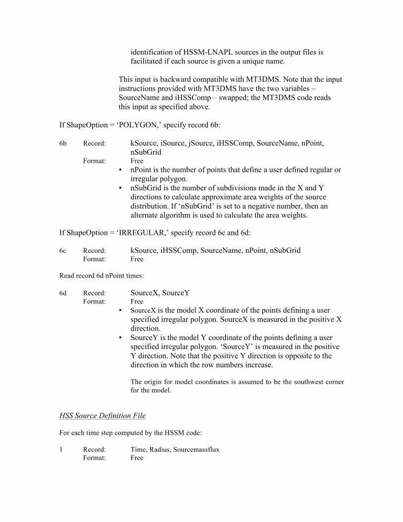
If ShapeOption is left blank, specify record 6a: 6a Record: kSource, iSource, jSource, iHSSComp, SourceName
Format: Free • kSource is the layer index of the initial model cell where a HSSM-
LNAPL source is located. • iSource is the row index of the initial model cell where a HSSM-
LNAPL source is located. • jSource is the column index of the initial model cell where a
HSSM-LNAPL source is located. • iHSSComp is the species index of the LNAPL source in a
multicomponent MT3D-USGS simulation. For example, if iSSComp = 2, the LNAPL source is intended for species number 2 included in the current simulation.
• SourceName is a string of 1 to 12 nonblank characters used to identify the HSSM-LNAPL source specified at location ‘kSource,’ ‘iSource,’ ‘jSource.’ The identifier need not be unique; however,
identification of HSSM-LNAPL sources in the output files is facilitated if each source is given a unique name.
This input is backward compatible with MT3DMS. Note that the input instructions provided with MT3DMS have the two variables – SourceName and iHSSComp – swapped; the MT3DMS code reads this input as specified above.
If ShapeOption = ‘POLYGON,’ specify record 6b: 6b Record: kSource, iSource, jSource, iHSSComp, SourceName, nPoint,
nSubGrid Format: Free
• nPoint is the number of points that define a user defined regular or irregular polygon.
• nSubGrid is the number of subdivisions made in the X and Y directions to calculate approximate area weights of the source distribution. If ‘nSubGrid’ is set to a negative number, then an alternate algorithm is used to calculate the area weights.
If ShapeOption = ‘IRREGULAR,’ specify record 6c and 6d: 6c Record: kSource, iHSSComp, SourceName, nPoint, nSubGrid
Format: Free
Read record 6d nPoint times: 6d Record: SourceX, SourceY
Format: Free • SourceX is the model X coordinate of the points defining a user
specified irregular polygon. SourceX is measured in the positive X direction.
• SourceY is the model Y coordinate of the points defining a user specified irregular polygon. ‘SourceY’ is measured in the positive Y direction. Note that the positive Y direction is opposite to the direction in which the row numbers increase. The origin for model coordinates is assumed to be the southwest corner for the model.
HSS Source Definition File
For each time step computed by the HSSM code: 1 Record: Time, Radius, Sourcemassflux
Format: Free
• Time is the total elapsed time since the beginning of simulation (unit: day).
• Radius is the radius of the source [L]. If zero or a negative value is assigned to radius_lnapl, the mass loading source is specified exclusively at the single finite-difference model cell (kSource, jSource, iSource) defined in the HSS input file. This input is required but ignored when ShapeOption is set to ‘IRREGULAR’.
• Sourcemassflux is the rate of contaminant mass flux dissolved into groundwater from the source (M/T).
LKT Package
Input to the Lake Transport Package is read from a file listed in the name file with “LKT” as the file type. The input file is needed only if lakes are simulated in the flow model using the LAK package in MODFLOW and a solution to the transport problem via and within the lake is desired. If lakes simulated using the LAK package of MODFLOW are only used as a boundary condition in MT3D-USGS, this package may not be used and the input for boundary concentration may be entered in the SSM package. For each simulation: 1 Record: NLKINIT, MXLKBC, ICBCLK, IETLAK Format: Free
• NLKINIT is an integer value equal to the number of simulated lakes as specified in the flow simulation.
• MXLKBC is an integer value that must be greater than or equal to the sum total of boundary conditions applied to each lake.
• ICBCLK is an integer value equal to the unit number on which lake-by-lake transport information will be printed. This unit number must appear in the NAM input file required for every MT3D-USGS simulation.
• IETLAK is an integer value specifying whether or not evaporation as simulated in the flow solution will act as a mass sink. = 0, Mass does not exit the model via simulated lake evaporation; ≠ 0, Mass may leave the lake via simulated lake evaporation;
2 Record: CINITLAK
Format: RARRAY • CINITLAK is a vector of real numbers representing the initial
concentrations in the simulated lakes. The length of the vector is equal to the number of simulated lakes, NLKINIT. Initial lake concentrations should be in the same order as the lakes appearing in the LAK input file corresponding to the MODFLOW simulation.
For each stress period: 3 Record: NTMP Format: I10
• NTMP is an integer value corresponding to the number of specified lake boundary conditions to follow. For the first stress period, this value must be greater than or equal to zero, but may be less than zero in subsequent stress periods.
If NTMP >= 0, NTMP is the number of lake boundary conditions. If NTMP = -1, lake boundary conditions from the previous stress period are
reused for the current stress period. (Read item 4 for each NTMP boundary condition) 4 Record: ILKBC, ILKBCTYP, (CBCLK(n), n=1, NCOMP) Format: Free
• ILKBC is an integer value that is the lake number for which the current boundary condition will be specified
• ILKBCTYP is an integer value that specifies, for ILKBC, what the boundary condition type is: = 1, a precipitation boundary condition. If precipitation to lakes is
simulated in the flow model and a non-zero concentration (default is zero) is associated with it, use ILKBCTYP = 1;
= 2, a runoff boundary condition. If runoff specified in the LAK package of MODFLOW has a non-zero concentration (default is zero) associated with it, use ILKBCTYP = 2. This input is not the same thing as runoff simulated in the UZF1 package and routed to a lake (or stream) using the IRNBND array.
• CBCLK is the specified concentration for the current boundary
condition. One entry (on the same line) per species.
RCT Package
Input to the Chemical Reaction Package is read on unit INRCT = 8, which is preset in the main program. The input file is needed only if chemical reactions are simulated. In addition, the option for modeling transport in a dual-domain system is specified through this file. For each simulation: 1 Record: ISOTHM, IREACT, IRCTOP, IGETSC, IREACTION
Format: 6I10 • ISOTHM is a flag indicating which type of sorption (or dual-
domain mass transfer) is simulated: = 0, no sorption is simulated; =1, Linear isotherm (equilibrium-controlled); =2, Freundlich isotherm (equilibrium-controlled); =3, Langmuir isotherm (equilibrium-controlled); =4, First-order kinetic sorption (nonequilibrium);
=5, Dual-domain mass transfer (without sorption); =6, Dual-domain mass transfer (with sorption). =-6, Dual-domain mass transfer (with different sorption coefficients in mobile and immobile domains).
• IREACT is a flag indicating which type of kinetic rate reaction is simulated: IREACT = 0, no kinetic rate reaction is simulated; IREACT = 1, first-order irreversible reaction; IREACT = 2, MONOD kinetic reaction is simulated; IREACT = 3, first-order chain reaction is simulated. IREACT = 100, zeroth-order reaction (decay or production) Note that options 1 and 2 are not intended for modeling chemical reactions between species.
• IRCTOP is an integer flag indicating how reaction variables are entered: IRCTOP ≥ 2, all reaction variables are specified as 3-D arrays on a cell-by-cell basis. IRCTOP < 2, all reaction variables are specified as a 1-D array with each value in the array corresponding to a single layer. This option is mainly for retaining compatibility with the previous versions of MT3DMS.
• IGETSC is an integer flag indicating whether the initial concentration for the non-equilibrium sorbed or immobile phase of all species should be read when non-equilibrium sorption (ISOTHM = 4) or dual-domain mass transfer (ISOTHM = 5 or 6) is simulated: IGETSC = 0, the initial concentration for the sorbed or immobile phase is not read. By default, the sorbed phase is assumed to be in equilibrium with the dissolved phase (ISOTHM = 4), and the immobile domain is assumed to have zero concentration (ISOTHM = 5 or 6). IGETSC > 0, the initial concentration for the sorbed phase or immobile liquid phase of all species will be read.
• IREACTION is an integer flag to select a reaction module. At least
2 species must be simulated when this option is used. Additional input is needed in needed when this option is used. If IREACTION=0, no reaction is simulated.
If IREACTION=1, instantaneous EA/ED reaction is simulated between an ED and an EA.
If IREACTION=2, kinetic reaction is simulated between multiple EAs and EDs.
•
(Enter 2A if ISOTHM=1, 2, 3, 4, 6, or -6; but not 5; OR if IREACTION=2) 2A Record: RHOB(NCOL,NROW) (one array for each layer)
Format: RARRAY • RHOB is the bulk density of the aquifer medium (unit, ML-3).
(Enter 2B if ISOTHM = 5, 6, or -6) 2B Record: PRSITY2(NCOL,NROW) (one array for each layer)
Format: RARRAY • PRSITY2 is the porosity of the immobile domain, i.e., the ratio of pore
spaces filled with immobile fluids over the bulk volume of the aquifer medium, when the simulation is intended to represent a dual-domain system.
(Enter 2C for each species if IGETSC > 0) 2C Record: SRCONC(NCOL,NROW) (one array for each layer)
Format: RARRAY • SRCONC is the user-specified initial concentration for the sorbed phase
of a particular species if ISOTHM = 4 (unit, MM-1). Note that for equilibrium-controlled sorption, the initial concentration for the sorbed phase cannot be specified. SRCONC is the user-specified initial concentration for the immobile liquid phase if ISOTHM = 5 or 6 (unit, ML-3).
(Enter 3a for each species if ISOTHM ≠ 0) 3a Record: SP1(NCOL,NROW) (one array for each layer)
Format: RARRAY • SP1 is the first sorption parameter. The use of SP1 depends on the type
of sorption selected (i.e., the value of ISOTHM): For linear sorption (ISOTHM = 1) and nonequilibrium sorption (ISOTHM = 4), SP1 is the distribution coefficient (Kd) (unit, L3M-1). For Freundlich sorption (ISOTHM = 2), SP1 is the Freundlich equilibrium constant (Kf) (the unit depends on the Freundlich exponent a).
For Langmuir sorption (ISOTHM = 3), SP1 is the Langmuir equilibrium constant (Kl) (unit, L3M-1). For dual-domain mass transfer without sorption (ISOTHM = 5), SP1 is not used, but still must be entered. For dual-domain mass transfer with sorption (ISOTHM = 6), SP1 is also the distribution coefficient (Kd) (unit, L3M-1). For dual-domain mass transfer with sorption (ISOTHM = -6), SP1 is the mobile domain distribution coefficient (
mdK ) (unit, L3M-1).
(Enter 3b for each species if ISOTHM = -6) 3b Record: SP1IM(NCOL,NROW) (one array for each layer)
Format: RARRAY • SP1IM is the immobile domain partitioning/distribution coefficient
(imd
K ) (unit, L3M-1). This option is entered only if ISOTHM = -6, i.e. if a different partitioning coefficient is simulated for the immobile domain.
(Enter 4 for each species if ISOTHM > 0) 4 Record: SP2(NCOL,NROW) (one array for each layer)
Format: RARRAY • SP2 is the second sorption or dual-domain model parameter. The use of
SP2 depends on the type of sorption or dual-domain model selected: For linear sorption (ISOTHM = 1), SP2 is read but not used. For Freundlich sorption (ISOTHM = 2), SP2 is the Freundlich exponent a. For Langmuir sorption (ISOTHM = 3), SP2 is the total concentration of the sorption sites available (S) (unit, MM-1). For non-equilibrium sorption (ISOTHM = 4), SP2 is the first-order mass transfer rate between the dissolved and sorbed phases (unit, T-1). For dual-domain mass transfer (ISOTHM = 5 or 6), SP2 is the first-order mass transfer rate between the two domains (unit, T-1).
(Enter 5 for each species if IREACT > 0) 5 Record: RC1(NCOL, NROW) (one array for each layer)
Format: RARRAY • If IREACT = 1 or 3, RC1 is the first-order reaction rate for the
dissolved (liquid) phase (unit, T-1). If a dual-domain system is simulated, the reaction rates for the liquid phase in the mobile and immobile domains are assumed to be equal.
• If IREACT = 2 (MONOD kinetics), RC1 is the product of total microbial concentration, Mt (unit, ML-3) and the maximum specific growth rate of the bacterium, umax (unit, T-1).
• If IREACT = 100 (zeroth-order decay or production), RC1 is the zeroth-order reaction rate coefficient for the dissolved (liquid) phase (ML-3T-1) (positive for decay and negative for production). If a dual-domain system is simulated, the rate coefficients for the liquid phase in the mobile and immobile domains are assumed equal.
(Enter 6 for each species if IREACT > 0) 6 Record: RC2(NCOL, NROW) (one array for each layer)
Format: RARRAY • If IREACT = 1 (first-order kinetic reactions) RC2 is the first-order
reaction rate for the sorbed phase (unit, T-1). If a dual-domain system is simulated, the reaction rates for the sorbed phase in the mobile and immobile domains are assumed to be equal. Generally, if the reaction is radioactive decay, RC2 should be set equal to RC1, while for biodegradation, RC2 may be different from RC1. Note that RC2 is read but not used, if no sorption is included in the simulation.
• If IREACT=100 (zeroth-order decay or production), RC2 is the zeroth-order reaction rate coefficient for the sorbed (solid) phase (MM-1T-1) (positive for decay and negative for production). If a dual-domain system is simulated, the rate coefficients for the liquid phase in the mobile and immobile domains are assumed equal.
(Enter 7 for each species if IREACT = 2) 7 Record: RC3(NCOL, NROW) (one array for each layer)
Format: RARRAY • RC3 is the half-saturation constant sK (unit, ML-3). Note that RC3 is
read and used only if IREACT = 2 option to simulate MONOD kinetics is invoked.
(Enter 8 if IREACT = 3, one line for each species) 8 Record: YLD(NSPEC-1)
Format: F10.0 • YLD is the yield coefficient between species. The first value in the array
is for the reaction between species 1 and species 2; the second value for the reaction between species 2 and 3; and so on. Note that YLD is read and used only if IREACT = 3 option to simulate first-order chain reaction is invoked. This option is only available when more than one species are simulated.
(Enter 9a if IREACTION=1; or if IREACT=90 or 91) 9a Record: IED, IEA, F
Format: 2I10, F10.0 • IED is the species number representing the electron donor participating
in the EA/ED reaction. • IEA is the species number representing the electron acceptor
participating in the EA/ED reaction. • F is the stoiciometric ratio in the simulated equation
ED + F*EA à Product
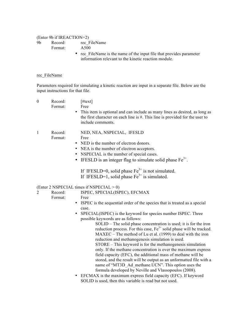
(Enter 9b if IREACTION=2) 9b Record: rec_FileName
Format: A500 • rec_FileName is the name of the input file that provides parameter
information relevant to the kinetic reaction module. rec_FileName Parameters required for simulating a kinetic reaction are input in a separate file. Below are the input instructions for that file. 0 Record: [#text]
Format: Free • This item is optional and can include as many lines as desired, as long as
the first character on each line is #. This line is provided for the user to include comments.
1 Record: NED, NEA, NSPECIAL, IFESLD
Format: Free • NED is the number of electron donors. • NEA is the number of electron acceptors. • NSPECIAL is the number of special cases. • IFESLD is an integer flag to simulate solid phase Fe3+.
If IFESLD=0, solid phase Fe3+ is not simulated. If IFESLD=1, solid phase Fe3+ is simulated.
(Enter 2 NSPECIAL times if NSPECIAL > 0) 2 Record: ISPEC, SPECIAL(ISPEC), EFCMAX
Format: Free • ISPEC is the sequential order of the species that is treated as a special
case. • SPECIAL(ISPEC) is the keyword for species number ISPEC. Three
possible keywords are as follows: SOLID – The solid phase concentration is used; it is for the iron reduction process. For this case, Fe3+ solid phase will be tracked. MAXEC – The method of Lu et al. (1999) to deal with the iron reduction and methanogenesis simulation is used. STORE – This keyword is for the methanogenesis simulation only. If the methane concentration is over the maximum express field capacity (EFC), the additional mass of methane will be stored, and the result will be output as an unformatted file with a name of “MT3D_Ad_methane.UCN”. This option uses the formula developed by Neville and Vlassopoulos (2008).
• EFCMAX is the maximum express field capacity (EFC). If keyword SOLID is used, then this variable is read but not used.
(Enter 3 NEA times) 3 Record: HSC, IC
Format: Free • HSC is the half saturation constant. • IC is the inhibition constants.
(Enter 4 NEA times) 4 Record: DECAYRATE(1:NED)
Format: Free • DECAYRATE is the decay rate of each electron acceptor corresponding
to each electron donor. (Enter 5 NEA+NED times) 4 Record: YIELDC(1:NED)
Format: Free • YIELDC is the yield coefficient of each component corresponding to
each electron donor.
New input requirements
Below is a discussion on input requirements for the revised MT3D-USGS program for the new reaction package. This section describes in general terms, the input variables required to complete a simulation that considers multiple electron donors and electron acceptors, and production of a lower-order ED from the decay of a higher-order ED. The discussion uses a hypothetical system comprising three EDs and five EAs such that nED = 3, nEA = 5, and nED + nEA = 8. In this hypothetical, the three EAs are (1) benzene, (2) MTBE, and (3) TBA. The simulated relationships are as follows: (1) degradation of benzene, without formation of a product; (2) degradation of MTBE with formation of TBA [yield coefficient = 1]; and, (3) degradation of TBA, without formation of a product. This simulation requires that the following inputs be provided:
1. First order decay rates for each ED corresponding to each TEAP
2. Yield coefficients corresponding to:
a. The consumption of each EA due to the degradation of each ED
b. The production of a lower-order ED from the degradation of a higher-order ED
3. Inhibition constants
4. Half-saturation constants
The inputs for such a simulation are provided as tables, or matrices, in the following order: decay rates, yield coefficients, inhibition constants, and half-saturation constants. If it is assumed that the half saturation constant expresses the concentration minimum at which any activity can occur for that species – i.e., that a single-valued half-saturation
constant applies to each combination of ED and EA - the half-saturation constants can be provided as a vector with dimensions nED+nEA. Figure 8 is an example matrix of nED rows and nEA columns that identifies required inputs for the remaining reaction parameters, and Figure 9 is an example matrix with nED + nEA rows by nED + nEA columns that the user must fill in when simulating multiple EA and ED reactions. Finally, Figure 10 shows a non-square, non-symetric matrix with nED rows and nED + nEA colums that the user must specify when simulating multiple ED and EA reactions.
Table 2 – A matrix of maximum first order decay rates are required input for simulating multiple EA and ED reactions, an example of which is shown here. Figure 9, below, also shows input requirements for this type of simulation.
O2 NO3 FE2 SO4 CH3 BTEX Y Y Y Y Y MTBE Y Y Y Y Y TBA Y Y Y Y Y
Table 3 – A matrix of yield coefficients is required for simulating multiple EA and ED reactions. Although in the general case the matrix could possess nED+nEA rows, on most occasions the matrix will actually possess nED rows. The entry in the corresponding cell indicates whether a value needs to be provided. If a value must be provided, it is the rate of the column species production/consumption due to degradation of 1 unit of the row species. The entries “+”, “-”, and “N” represent production, consumption, and no relationship, respectively.
BTEX MTBE TBA O2 NO3 FE2 SO4 CH3 BTEX N N N - - + - + MTBE N N + - - + - + TBA N N N - - + - + O2 N N N N N N N N
NO3 N N N N N N N N FE2 N N N N N N N N SO4 N N N N N N N N CH3 N N N N N N N N
Table 4 – A matrix of required inhibition constants that must be specified when simulating multiple EA and ED reactions. Although in the general case the matrix could possess nED rows, on most occasions the matrix will actually possess only one row; that is, each species in the reaction possesses a single inhibition constant.
BTEX MTBE TBA O2 NO3 FE2 SO4 CH3 BTEX N N N + + + + + MTBE + N N + + + + + TBA + + N + + + + +
Mass depletion from the system is reported in the global mass balance summary in the standard output file as a new term called “DECAY OR BIODEGRADATION”. Users seeking to make use of this option are referred to the input instructions for its implementation.
SFT Package
Input for the SFT package is read from a file listed in the name file with “SFT” as the file type. The input file is needed only if streams simulated using the SFR2 package in MODFLOW are activated and a solution to the surface water network transport problem is desired. If streams simulated using the SFR2 package of MODFLOW are only used as a boundary condition in MT3D-USGS, this package may not be used and the input for boundary concentration may be entered in the SSM package. Due to the explicit coupling of the transport solution of stream nodes and groundwater nodes, it is imperative that the number of outer iterations (MXITER) for the groundwater transport solution be set greater than 1. For each simulation: 1 Record: NSFINIT, MXSFBC, ICBCSF, IOUTOBS, IETSFR
Format: Free • NSFINIT is the number of simulated stream reaches (in SFR2, the
number of stream reaches is greater than or equal to the number of stream segments). This is equal to NSTRM found on the first line of the SFR2 input file. If NSFINIT > 0 then surface-water transport is solved in the stream network while taking into account groundwater exchange and precipitation and evaporation sources and sinks. Otherwise, if NSFINIT < 0, the surface-water network as represented by the SFR2 flow package merely acts as a boundary condition to the groundwater transport problem; transport in the surface-water network is not simulated.
• MXSFBC is the maximum number of stream boundary conditions. • ICBCSF is an integer value that directs MT3D-USGS to write reach-by-
reach concentration information to unit ICBCSF. This flag is set to 0 and is not used in the first release of MT3D-USGS (version 1.0).
• IOUTOBS is an integer value that is the unit number of the output file for simulated concentrations at specified gage locations. The NAM file must also list the unit number to which observation information will be written.
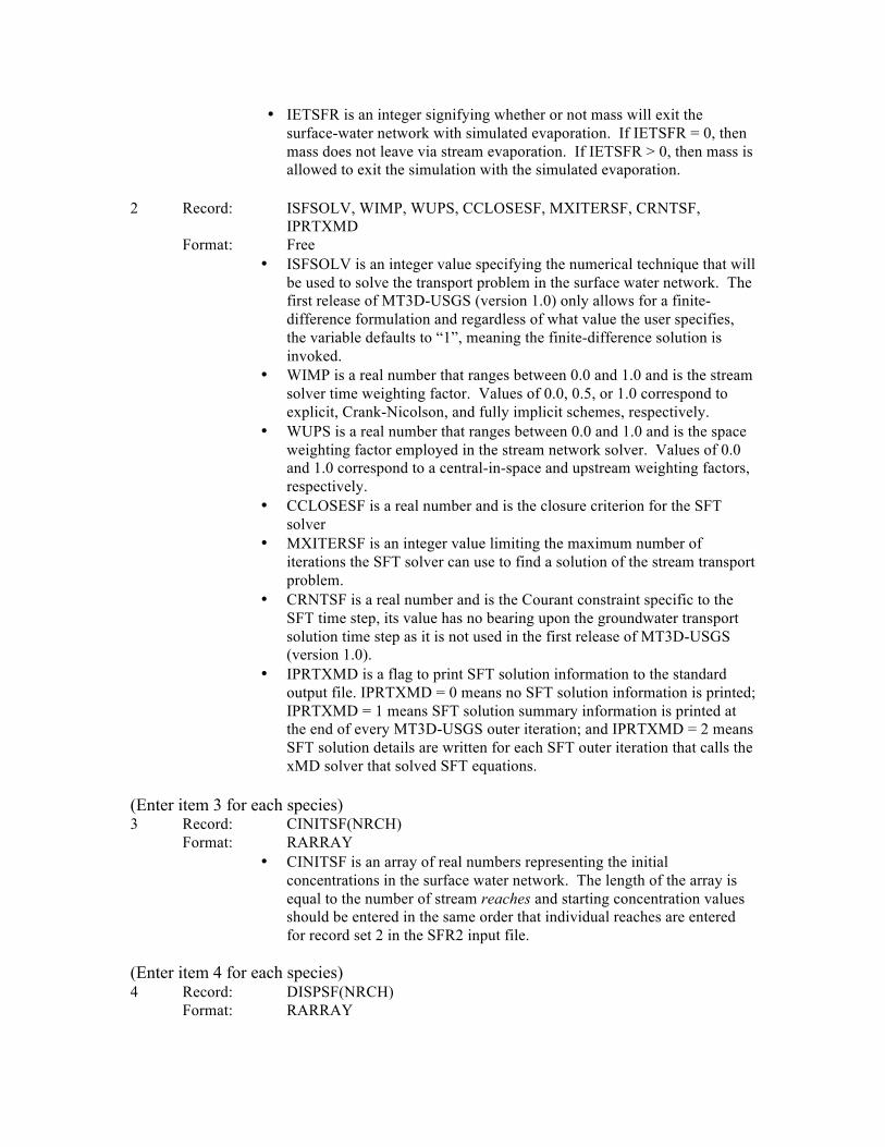
• IETSFR is an integer signifying whether or not mass will exit the surface-water network with simulated evaporation. If IETSFR = 0, then mass does not leave via stream evaporation. If IETSFR > 0, then mass is allowed to exit the simulation with the simulated evaporation.
Format: Free • ISFSOLV is an integer value specifying the numerical technique that will
be used to solve the transport problem in the surface water network. The first release of MT3D-USGS (version 1.0) only allows for a finite-difference formulation and regardless of what value the user specifies, the variable defaults to “1”, meaning the finite-difference solution is invoked.
• WIMP is a real number that ranges between 0.0 and 1.0 and is the stream solver time weighting factor. Values of 0.0, 0.5, or 1.0 correspond to explicit, Crank-Nicolson, and fully implicit schemes, respectively.
• WUPS is a real number that ranges between 0.0 and 1.0 and is the space weighting factor employed in the stream network solver. Values of 0.0 and 1.0 correspond to a central-in-space and upstream weighting factors, respectively.
• CCLOSESF is a real number and is the closure criterion for the SFT solver
• MXITERSF is an integer value limiting the maximum number of iterations the SFT solver can use to find a solution of the stream transport problem.
• CRNTSF is a real number and is the Courant constraint specific to the SFT time step, its value has no bearing upon the groundwater transport solution time step as it is not used in the first release of MT3D-USGS (version 1.0).
• IPRTXMD is a flag to print SFT solution information to the standard output file. IPRTXMD = 0 means no SFT solution information is printed; IPRTXMD = 1 means SFT solution summary information is printed at the end of every MT3D-USGS outer iteration; and IPRTXMD = 2 means SFT solution details are written for each SFT outer iteration that calls the xMD solver that solved SFT equations.
(Enter item 3 for each species) 3 Record: CINITSF(NRCH)
Format: RARRAY • CINITSF is an array of real numbers representing the initial
concentrations in the surface water network. The length of the array is equal to the number of stream reaches and starting concentration values should be entered in the same order that individual reaches are entered for record set 2 in the SFR2 input file.
(Enter item 4 for each species) 4 Record: DISPSF(NRCH) Format: RARRAY
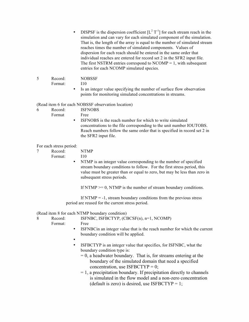
• DISPSF is the dispersion coefficient [L2 T-1] for each stream reach in the simulation and can vary for each simulated component of the simulation. That is, the length of the array is equal to the number of simulated stream reaches times the number of simulated components. Values of dispersion for each reach should be entered in the same order that individual reaches are entered for record set 2 in the SFR2 input file. The first NSTRM entries correspond to NCOMP = 1, with subsequent entries for each NCOMP simulated species.
5 Record: NOBSSF Format: I10
• Is an integer value specifying the number of surface flow observation points for monitoring simulated concentrations in streams.
(Read item 6 for each NOBSSF observation location) 6 Record: ISFNOBS Format Free
• ISFNOBS is the reach number for which to write simulated concentrations to the file corresponding to the unit number IOUTOBS. Reach numbers follow the same order that is specified in record set 2 in the SFR2 input file.
For each stress period: 7 Record: NTMP Format: I10
• NTMP is an integer value corresponding to the number of specified stream boundary conditions to follow. For the first stress period, this value must be greater than or equal to zero, but may be less than zero in subsequent stress periods.
If NTMP >= 0, NTMP is the number of stream boundary conditions.
If NTMP = -1, stream boundary conditions from the previous stress
period are reused for the current stress period. (Read item 8 for each NTMP boundary condition) 8 Record: ISFNBC, ISFBCTYP, (CBCSF(n), n=1, NCOMP) Format: Free
• ISFNBCin an integer value that is the reach number for which the current boundary condition will be applied.
• • ISFBCTYP is an integer value that specifies, for ISFNBC, what the
boundary condition type is: = 0, a headwater boundary. That is, for streams entering at the
boundary of the simulated domain that need a specified concentration, use ISFBCTYP = 0;
= 1, a precipitation boundary. If precipitation directly to channels is simulated in the flow model and a non-zero concentration (default is zero) is desired, use ISFBCTYP = 1;
= 2, a runoff boundary condition associated with the SFR2 package of MODFLOW. This is not the same thing as runoff simulated in the UZF1 package and routed to a stream (or lake) using the IRNBND array. Users who specify runoff in the SFR2 input via the RUNOFF variable appearing in either record sets 4b or 6a and want to assign a non-zero concentration (default is zero) associated with this specified source, use ISFBCTYP=2;
= 3, a constant-concentration boundary. Any reach number may be set equal to a constant concentration boundary condition.
= 4, • CBCSF is a real number and is the specified concentration associated
with the current boundary condition entry. Repeat CBCSF for each simulated species (NCOMP).
SSM Package
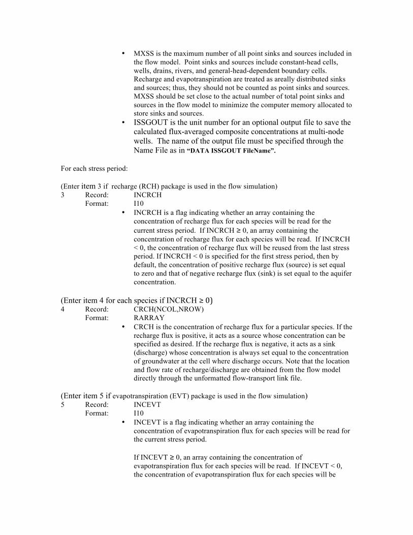
Input to the Sink & Source Mixing package is read on unit INSSM=4, which is preset in the main program. The input file is needed if any sink or source option is used in the flow model, including the constant-head, general-head, river, drain, recharge, evapotranspiration, well, multi-node well, stream, lake, and unsaturated zone packages. For each simulation: 1 Record: FWEL, FDRN, FRCH, FEVT, FRIV, FGHB
Format: 10L2 • These logical flags are no longer needed as the status of various
flow sink/source packages is obtained by MT3D-USGS through the Flow-Transport Link File produced by MODFLOW. However, a dummy input line must still be specified in the input file. A blank line is acceptable.
When MODFLOW-NWT is used to obtain flow solutions for MT3D-USGS, the LMT package for MODFLOW will store appropriate values for these flags in the formatted and unformatted flow-transport link file. If these flags are not specified correctly here, MT3DMS will issue a warning, reset the flags to correct values, and proceed with the simulation.
Note that the add-on package Stream package (STR) is supported through the River option. This is done by associating the River option in MT3D-USGS with the STR package instead of the RIV package in MODFLOW. For this reason, the RIV and STR packages cannot be used concurrently in the same MODFLOW simulation.
2 Record: MXSS, ISSGOUT
Format: 2I10
• MXSS is the maximum number of all point sinks and sources included in the flow model. Point sinks and sources include constant-head cells, wells, drains, rivers, and general-head-dependent boundary cells. Recharge and evapotranspiration are treated as areally distributed sinks and sources; thus, they should not be counted as point sinks and sources. MXSS should be set close to the actual number of total point sinks and sources in the flow model to minimize the computer memory allocated to store sinks and sources.
• ISSGOUT is the unit number for an optional output file to save the calculated flux-averaged composite concentrations at multi-node wells. The name of the output file must be specified through the Name File as in “DATA ISSGOUT FileName”.
For each stress period: (Enter item 3 if recharge (RCH) package is used in the flow simulation) 3 Record: INCRCH
Format: I10 • INCRCH is a flag indicating whether an array containing the
concentration of recharge flux for each species will be read for the current stress period. If INCRCH ≥ 0, an array containing the concentration of recharge flux for each species will be read. If INCRCH < 0, the concentration of recharge flux will be reused from the last stress period. If INCRCH < 0 is specified for the first stress period, then by default, the concentration of positive recharge flux (source) is set equal to zero and that of negative recharge flux (sink) is set equal to the aquifer concentration.
(Enter item 4 for each species if INCRCH ≥ 0) 4 Record: CRCH(NCOL,NROW)
Format: RARRAY • CRCH is the concentration of recharge flux for a particular species. If the
recharge flux is positive, it acts as a source whose concentration can be specified as desired. If the recharge flux is negative, it acts as a sink (discharge) whose concentration is always set equal to the concentration of groundwater at the cell where discharge occurs. Note that the location and flow rate of recharge/discharge are obtained from the flow model directly through the unformatted flow-transport link file.
(Enter item 5 if evapotranspiration (EVT) package is used in the flow simulation) 5 Record: INCEVT
Format: I10 • INCEVT is a flag indicating whether an array containing the
concentration of evapotranspiration flux for each species will be read for the current stress period.
If INCEVT ≥ 0, an array containing the concentration of evapotranspiration flux for each species will be read. If INCEVT < 0, the concentration of evapotranspiration flux for each species will be
reused from the last stress period. If INCEVT < 0 is specified for the first stress period, then by default, the concentration of negative evapotranspiration flux (sink) is set to the aquifer concentration, while the concentration of positive evapotranspiration flux (source) is set to zero.
(Enter item 6 for each species if INCEVT ≥ 0) 6 Record: CEVT(NCOL,NROW)
Format: RARRAY • CEVT is the concentration of evapotranspiration flux for a particular
species. Evapotranspiration is the only type of sink whose concentration may be specified externally. Note that the concentration of a sink cannot be greater than that of the aquifer at the sink cell. Thus, if the sink concentration is specified greater than that of the aquifer, it is automatically set equal to the concentration of the aquifer. Also note that the location and flow rate of evapotranspiration are obtained from the flow model directly through the unformatted flow-transport link file.
(Enter items 7-10 if unsaturated zone (UZF) package is used in the flow simulation) 7 Record: INCUZF
Format: I10 • INCUZF is a flag indicating whether an array containing the
concentration of infiltration flux for each species will be read for the current stress period. If INCUZF ≥ 0, an array containing the concentration of infiltration flux for each species will be read. If INCUZF < 0, the concentration of infiltration flux will be reused from the last stress period.
(Enter item 8 for each species if INCUZF ≥ 0) 8 Record: CUZRCH (NCOL,NROW)
Format: RARRAY • CUZRCH is the concentration of infiltration flux for a particular species.
Note that the location and flow rate are obtained from the flow model directly through the unformatted flow-transport link file.
9 Record: INCGWET Format: I10
• INCGWET is a flag indicating whether an array containing the concentration of seepage flux for each species will be read for the current stress period.
If INCGWET ≥ 0, an array containing the concentration of seepage flux for each species will be read. If INCGWET ≥ 0, the concentration of seepage flux for each species will be reused from the last stress period. If INCGWET < 0, the concentration of infiltration flux will be reused from the last stress period.
(Enter item 10 for each species if INCEVT ≥ 0) 10 Record: CGWET (NCOL,NROW)
Format: RARRAY CGWET is the concentration of seepage flux for a particular species. Note that the concentration of a sink cannot be greater than that of the aquifer at the sink cell. Thus, if the sink concentration is specified greater than that of the aquifer, it is automatically set equal to the concentration of the aquifer. Also note that the location and flow rate of seepage are obtained from the flow model directly through the unformatted flow-transport link file.
11 Record: NSS
Format: I10 • NSS is the number of point sources whose concentrations need to be
specified. By default, unspecified point sources are assumed to have zero concentration. (The concentration of point sinks is always set equal to the concentration of groundwater at the sink location.)
Note that in MT3DMS, point sources are generalized to include not only those associated with a flow rate in the flow model, but also those independent of the flow solution. This type of “mass-loading” sources may be used to include contaminant sources which have minimal effects on the hydraulics of the flow field.
(Enter item 12 NSS times if NSS > 0) 12 Record: KSS, ISS, JSS, CSS, ITYPE, (CSSMS(n), n=1, NCOMP)
Format: 3I10, F10.0, I10, [free] • KSS, ISS, JSS are the cell indices (layer, row, column) of the point
source for which a concentration needs to be specified for each species.
Special cases for KSS, ISS, and JSS are as follows: • KSS must be set to 0, to implement a constant concentration
boundary (ITYPE = -1) to be applied on the same layer that the recharge is applied.
• To specify lake concentration (ITYPE = 26), KSS and ISS must be set to zero, and JSS must be set equal to the lake number for which the concentration is specified. Groundwater cells gaining mass from the lake JSS are internally identified based on information provided via the flow link file, and the same lake concentration is used for all gaining groundwater cells connected to the lake specified using JSS.
• CSS is the specified source concentration or mass-loading rate,
depending on the value of ITYPE, in a single-species simulation. For a multispecies simulation, CSS is not used, but a dummy value still needs to be entered here.
Note that for most types of sources, CSS is interpreted as the source concentration with the unit of mass per unit volume (ML-3), which, when multiplied by its corresponding flow rate (L3T-1) from the flow model, yields the mass-loading rate (MT-1) of the source.
For a special type of sources (ITYPE = 15), CSS is taken directly as the mass-loading rate (MT-1) of the source so that no flow rate is required from the flow model.
Furthermore, if the source is specified as a constant concentration cell (ITYPE = -1), the specified value of CSS is assigned directly as the concentration of the designated cell. If the designated cell is also associated with a sink/source term in the flow model, the flow rate is not used.
• ITYPE is an integer indicating the type of the point source as listed below: ITYPE = 1, constant-head cell;
= 2, well; = 3, drain (note that in MODFLOW conventions, a drain is
always a sink, thus, the concentration for drains cannot be specified if the flow solution is from MODFLOW);
= 4, river; = 5, general-head-dependent boundary cell; = 15, mass-loading source; = -1, constant-concentration cell; = 21, stream-flow routing (STR); = 22, reservoir; = 23, specified flow and head boundary; = 26, lake; = 27, multi-node well; = 28, drain with return flow; = 30, stream-flow routing (SFR). For informational purposes, other reserved ITYPE unit numbers include 7, 8, 29, and 31 for recharge, evapotranspiration, evapotranspiration with segments, and unsaturated-zone flow, respectively. Only the numbers listed above may be entered.
• Ever since an earlier version of MT3DMS (v5.2), users can specify the input concentration of an injection well (ISSTYPE=2), i.e., CSS or CSSMS, as a negative integer code (IC). The absolute value of the integer code is the single cell location indicator of the extraction well whose output concentration is used as the input concentration for the injection well. For an extraction well located at layer K, row I, and column J, IC is computed as,
( ) ( ) JINCOLKNROWNCOLIC +−×+−××= 11
where NCOL and NROW are the total numbers of columns and rows.
• (CSSMS(n), n=1, NCOMP) defines the concentrations of a point source
for multispecies simulation with NCOMP > 1. In a multispecies simulation, it is necessary to define the concentrations of all species
associated with a point source. As an example, if a chemical of a certain species is injected into a multispecies system, the concentration of that species is assigned a value greater than zero while the concentrations of all other species are assigned zero. CSSMS(n) can be entered in free format, separated by a comma or space between values. Several important notes on assigning concentration for the constant-concentration condition (ITYPE = -1) are listed below:
The constant-concentration condition defined in this input file takes precedence to that defined in the Basic Transport Package input file. In a multiple stress period simulation, a constant-concentration cell, once defined, will remain a constant-concentration cell in the duration of the simulation, but its concentration value can be specified to vary in different stress periods. In a multispecies simulation, if it is only necessary to define different constant-concentration conditions for selected species at the same cell location, specify the desired concentrations for those species, and assign a negative value for all other species. The negative value is a flag used by MT3DMS to skip assigning the constant-concentration condition for the designated species.
TOB Package
Are we going to stick with this package? And if so, for completeness-sake, do we want to bring in the instructions from the supplemental materials to codify all input instructions?
UZT Package
Input for the UZT package is read from a file listed in the name file with “UZT” as the file type. The input data are read in free format. Input instructions are given below For each simulation: 1 Record: HEADNG(1)
Format: A80 • HEADNG(1) is the first line of any title or heading for the simulation
run. This line can be repeated as many time as desired. The first character on the line (position 0) must be ‘#’.
2 Record: ICBCUZ, IET
Format: Free • • ICBCUZ is the unit number to which unsaturated-zone concentration
will be written out. • IET is a flag that indicates whether or not ET is being simulated in the
UZF1 flow package. If ET is not being simulated, IET informs the FMI
package not to look for UZET and GWET arrays in the flow-transport link file.
3 Record: IUZFBND(NROW,NCOL) (one array for each layer)
Format: Free • IUZFBND is an array of integer values specifying which row/column
indicies variably-saturated transport will be simulated in. IUZFBND > 0 indicates that variably-saturated transport will be simulated. IUZFBND = 0 means variably-saturated transport will not be simulated. IUZFND < 0 corresponds to IUZFBND < 0 in the UZF1 input package, meaning that user-supplied values for FINF are specified recharge.
4 Record: WC(NROW,NCOL) (one array for each layer)
Format: Free • WC is an array of starting water contents. For cells above the water
table, this value can range between residual and saturated water contents. In cells below the water table, this value will be equal to saturated water content (i.e., effective porosity).
5 Record: SDH(NROW,NCOL) (one array for each layer)
Format: Free • SDH is the starting saturated thickness for each cell in the simulation.
SDH = 0 in cells residing above the starting water table, is equal to the cell thickness for cells where the water table is above the top elevation of the cell. For cells in which the water table resides, SDH is equal to the water table elevation minus the bottom elevation of the cell.
For each stress period: 6 Record: INCUZINF
Format: I10 • INCUZINF is a flag indicating whether an array containing the
concentration of infiltrating (FINF) flux for each species will be read for the current stress period. If INCUZINF ≥ 0, an array containing the concentration of infiltrating flux for each species will be read. If INCUZINF < 0, the concentration of infiltrating flux will be reused from the previous stress period. If INCUZINF < 0 is specified for the first stress period, then by default the concentration of positive infiltrating flux (source) is set equal to zero. There is no possibility of a negative infiltration flux being specified. If infiltrating water is rejected due to an infiltration rate exceeding the vertical hydraulic conductivity, or because saturation is reached in the unsaturated zone and the water table is therefore at land surface, the concentration of the runoff will be equal to CUZINF specified next. The runoff is routed if IRNBND is specified in the MODFLOW simulation.
(Enter item 7 for each species if INCRCH ≥ 0) 7 Record: CUZINF
Format: RARRAY • CUZINF is the concentration of the infiltrating flux for a particular
species.
8 Record: INCUZET
Format: I10 • INCUZET is a flag indicating whether an array containing the
concentration of evapotranspiration flux originating from the unsaturated zone will be read for the current stress period.
If INCUZET ≥ 0, an array containing the concentration of evapotranspiration flux originating from the unsaturated zone for each species will be read. If INCUZET < 0, the concentration of evapotranspiration flux for each species will be reused from the last stress period. If INCUZET < 0 is specified for the first stress period, then by default, the concentration of negative evapotranspiration flux (sink) is set to the aquifer concentration, while the concentration of positive evapotranspiration flux (source) is set to zero.
(Enter item 9 for each species if INCUZET ≥ 0) 9 Record: CUZET
Format: RARRAY • CUZET is the concentration of ET fluxes originating from the
unsaturated zone. As a default, this array is set equal to 0 and only overridden if the user specifies INCUZET > 1. If empirical evidence suggest volatilization of simulated constituents from the unsaturated zone, this may be one mechanism for simulating this process, though it would depend on the amount of simulated ET originating from the unsaturated zone.
10 Record: INCGWET
Format: I10 • INCGWET is a flag indicating whether an array containing the
concentration of evapotranspiration flux originating from the saturated zone will be read for the current stress period.
If INCGWET ≥ 0, an array containing the concentration of evapotranspiration flux originating from the saturated zone for each species will be read. If INCGWET < 0, the concentration of evapotranspiration flux for each species will be reused from the last stress period. If INCUZET < 0 is specified for the first stress period, then by default, the concentration of negative evapotranspiration flux (sink) is set to the aquifer concentration, while the concentration of positive evapotranspiration flux (source) is set to zero.
(Enter item 11 for each species if INCGWET ≥ 0) 11 Record: CGWET
Format: RARRAY • CGWET is the concentration of ET fluxes originating from the saturated
zone. As a default, this array is set equal to 0 and only overridden if the user specifies INCUZET > 1.
Output
For a detailed description of output files and output generated by MT3DMS, please refer to the original MT3DMS manuals (Zheng and Wang, 1999; Zheng, 2010). Additional output generated by MT3D-USGS is described below. New options added in MT3D-USGS are echoed to the standard output files with a brief description.
Output Files
A number of output files are generated based on various options introduced in MT3D-USGS. The output files, their formats, and the options that produce the output files are as follows. CTO file The CTO file contains a well-by-well printout of the mass balance related to the CTS package. CTO file is a formatted ASCII output file optionally generated by modified MT3DMS. This file is generated if the flag ICTSOUT is set to a unit number when the CTS package is used. ICTSOUT can be set to zero if the CTO file is not desired. See the input instruction of CTS package for more details. CTO is the extension provided to the output file using the same filename that is specified for the CTS input file by replacing the file extension. The output to this file is printed in the following format. • Stress period, flow time step, transport time step, time step size, contaminant
treatment system (CTS) index, well index number, layer, row, column, species, flow rate, concentration, and mass.
• 3I10,1X,G14.7,6I10,3(1X,G14.7)
Budget Terms
CTS Mass Balance If the contaminant treatment system (CTS) package is implemented in a simulation, a separate overall mass balance that is specific to the treatment systems is reported in the standard output file. The treatment system specific mass balance reports separate terms for mass extracted from the groundwater system via extraction wells that enters the treatment systems, mass entering the treatment systems from external sources, mass addition or removal as a result of specified treatment options, mass leaving the treatment systems that is injected back into the groundwater system, and mass leaving the treatment
systems to external sinks. Mass entering and leaving a treatment system also appears in the global mass budget summary of the standard output file. SFT Mass Balance If the stream-flow transport (SFT) package is implemented in a simulation, a separate overall mass balance that is specific to the stream reaches is reported in the standard output file. Mass entering and leaving the stream nodes also appears in the global mass budget summary of the standard output file. LKT Mass Balance If the lake transport (LKT) package is implemented in a simulation, a separate overall mass balance that is specific to the lakes is reported in the standard output file. Mass entering and leaving the lakes also appears in the global mass budget summary of the standard output file. Mass Balance Summary In the modified version of MT3DMS, a few new terms were introduced to the global mass balance summary written to the standard output file. Following are the new terms that were added:
• If the contaminant treatment system (CTS) package is implemented in a simulation, a separate term is reported as ‘TREATMENT SYSTEM’ in the standard output file. The treatment system IN and OUT terms in the overall mass balance account for mass entering via injection wells and mass leaving via extraction wells that are associated with treatment systems respectively.
• Storage change due to flow solution was calculated but not reported in the original MT3DMS. This term however, was added to the total IN and total OUT reported in the standard output file. The term is reported as ‘MASS STOR (FLOW MODEL): ’ in the mass balance summary.
• If keyword OMITDRYCELLBUDGET is not invoked in the BTN file, then mass flowing through dry cells is included and reported to the standard output file mass balance summary. The term is reported as ‘INACTIVE CELLS(ICBND=0):’.
• If instantaneous EA/ED reaction is invoked, then the mass lost from the system as a result of the reaction is reported as ‘EA-ED REACTION:’ in the mass balance summary of the standard output file.
• If kinetic reaction is invoked, then the mass budget for the reaction terms is reported as ‘DECAY OR BIODEGRADATION’ in the mass balance summary of the standard output file.
• If UZF is used then mass associated with infiltration or discharge is reported as ‘INFILTRATION/DISCHARGE’ and mass associated with evapotranspiration from UZF is reported as ‘UZ AND GW ET’.
• SFR influx and out-flux terms are reported as ‘STREAM’ in the mass balance summary of the standard output file.
• LAK influx and out-flux terms are reported as ‘LAKE’ in the mass balance summary of the standard output file.