1

Chapter 1

INRODUCTION AND LITERATURE REVIEW

1.1 Introduction

The manufacturing process of any product, no matter how well designed or

carefully maintained, always involves a certain amount of variation in the production

conditions. This natural fluctuation, often called a “stable system of chance causes,” is

the cumulative effect of many small, essentially uncontrollable factors. Under these

conditions we say that the manufacturing process is in a state of statistical control.

Sometimes in the output of a production process, other forms of non-natural variability

occur, usually from three main sources. These include improper adjustments in

machines, operator errors, or defective raw material. This non-natural variability is

called “assignable causes,” and is generally larger than the natural variability. It

represents an unacceptable level of process performance and such process is said to be

out of control.

A control chart is a graphical technique used for continuous monitoring whether the

manufacturing process is in a state of statistical control or not. Its primary objective is to

quickly detect the formation of assignable causes of process shifts so that investigation

of the process and corrective measure may be taken before many nonconforming units

brought to you by COREView metadata, citation and similar papers at core.ac.uk

provided by KFUPM ePrints

2

are manufactured. Generally, control chart is an effective tool in eliminating process

variability as well as estimating the parameters of the production process.

Since the first work of Shewhart [65], the construction of quality control charts has

undergone series of modifications with new methods being suggested. Most of the

methods reported in the literature are based on simple random sampling (SRS), which to

certain extent is considerably less effective in estimating the population mean as

compared to new sampling technique such as ranked set sampling (RSS) and its

modifications, see McIntyre [34], Takahashi and Wakimoto [76], Muttlak [42], Samawi

et al [60]. The use of ranked set sampling (RSS) and median ranked set sampling

(MRSS) as a sampling plan to develop control charts for monitoring the process mean

was first suggested by Salazar and Sinha [59]. They showed that the new charts were

substantially better than those based on the traditional SRS. Also, Muttlak and Al-Sabah

[47] developed control charts based on RSS, MRSS and other modifications of RSS

namely: the extreme ranked set sampling (ERSS), paired ranked set sampling (PRSS)

and selected ranked set sampling (SRSS) and showed that all these charts dominates the

classical SRS control charts for means.

The performance of such control charts using RSS and some of its modifications

lead us to assume without loss of generality that further modifications of RSS could

produce better control charts than the traditional SRS. The emergence of double ranked

set sampling (DRSS), see Al-Saleh and Al-Kadiri [6], and other proposed sampling

techniques namely: median double ranked set sampling (MDRSS), double median

ranked set sampling (DMRSS) and extreme double ranked set sampling (EDRSS) which

3

have all proven to be more effective in estimating the population mean as compared to

SRS, RSS, ERSS, PRSS and SRSS may play significant role in the monitoring a

characteristic of manufacturing process. This is the primary interest that motivates us to

investigate this problem. Other things that lead to this study are the need to investigate

how fast a shift in process variability could be detected using these new sampling

techniques.

1.2 Literature Review

In this section, we review some of the works in the area of statistical quality control

as well as the ranked set sampling (RSS) and classified them into two separate groups.

1.2.1 Statistical Quality Control

Although quality control has been with us since when manufacturing began and

competition accompanied manufacturing but, its scientific foundation with respect to

how many sample units to inspect and what conclusion to draw from the result and the

eventual extension to statistical quality control took place relatively late. The beginning

of statistical quality control dates back to 1924, when Shewhart [65] introduced his first

control chart for the fractional nonconforming units. His first control chart monitors

whether the nonconforming fraction of a product remains within the control limits

during the time of observation or not.

After over twenty five years from the original work of Shewhart [65], Aroian and

Levene [3] proposed the first trials to determine the three decision parameters of a

4

control chart namely; sample size, control limit, and time between sampling. With the

aim of minimizing the number of product units when the process is out of control, they

noted that the frequency of the false alarms which depends on the time interval between

samples plays a greater role in the determination of the control limits than the

probability of those false alarms per sample.

Weiler [81], used sample size in constructing a model to minimize the average

amount of inspection before a process shift occurs. In his work, he had completely

avoided the time interval between samples and the probability of detecting the effect of

process shift. In other words, the average run length (ARL) when the process is out of

control was neglected.

None of these works had so far taken into consideration the costs related to false

alarm and defectives incurred while the manufacturing process is out of control. These

cost related problems and the frequency of shift between two processes were considered

in the works of Duncan [23], Barnard [10] and Barish & Hauser [9]. All these works

have a common goal of pursuing control strategies that will effectively minimize the

average total cost per time unit of the respective manufacturing and control system. But

while Duncan [23] considered models with only a single point out of control, Barnard

[10] and Barish & Hauser [9] works on models with numerous numbers of points which

are out of control.

Crowder [19] presented a numerical procedure for the computation of average run

lengths (ARL) of a control chart using the combination of individual measurement and

moving range chart based on two consecutive measurements. He supplied the exact

5

expression for ARL in integral form and its approximation in numerical form. He also

gave ARL values for several settings of control limits and shifts in the process mean and

standard deviation.

On the effect of non-normality on x and R , Chan, et al [15] used some symmetric

distribution to study the departure from normality by comparing the probabilities of

when x and R lies outside the 3-standrard-deviation and 2-standrard-deviation control

limits. They reported that when the tails of the underlying distribution are thin and tick,

then the control charts based on the assumption of normality will produce inaccurate

results.

Champ and Woodall [14] suggested the use of Markov chain to obtain run length of

Shahwart control charts with supplementary runs rules. They presented the average run

length for the Shahwart x charts with supplementary runs rules, Shahwart x charts, and

the cumulative sum (CUSUM) chart. It was observed that although the supplementary

runs rules had made the traditional Shawhart charts to be more effective, but not as

sensitive as CUSUM charts.

Cryer and Ryan [20] studied the estimation of sigma for individual observations

control charts using the moving range and observed that the method is not as effective as

to the use of sample standard deviation when the observations are independent and

normally distributed. With aid of some real chemical data, they showed that the moving

range approach could produce poor results when the observations are correlated.

On a study of detecting the shifts in the process mean using the control chart for

averages, Palm [55] studied how sensitive a chart is to a process mean shift using the

6

distribution of the run length. He produced a table of percentile values for the

distribution of the measurement carried out on outgoing products. In a related study,

Walker and Philpot [80] observed that although the run lengths are effective in detecting

shift problems, they however increase the probability of a false signal.

Saniga [62] presented a FORTRAN program for determining the parameters of

control limits as well as the sample size for designing an X and R charts. The program

was based on a statistical criterion that can be stated in terms average run length, or

probabilities of type I and type II errors.

In his study of shift in process mean, Costa [17] observed that the use of x with

variable sample interval (VSI) or / and variable sample size (VSS) to detect the process

shift in mean is much faster as compared to the traditional x charts. He extended his

work, Costa [18], to the cases where both the x and R charts are used in detecting shifts

and observed that the new VSI and VSS based charts have improved the rate at which

the shifts in mean and / or variance are detected.

Amin and Wolff [2] studied the average run length (ARL) properties of some

control procedure for monitoring the mean and variance of a process. Considering a

situation where the underlying distribution is a mixture of normal distribution, they

computed the ARL values for the X , R , and Extreme-value charts and show that the

later is the most efficient of the three charts when it is targeted at detecting the presence

of mixture alternatives.

Roes and Does [58] discussed the use of an analysis of variance model in

constructing control charts with smaller variance. Using different estimators of

7

variability, they developed control charts for the mean and linear contrasts and also

provided a lead for the construction and evaluation of the charts.

Salazar and Sinha [59] constructed X - control chart based on ranked set samples

considering normal population and various shift values. Using visual comparison and

Monte Carlo simulation for the computation of average run length, they show that RSS

and median ranked set sampling (MRSS), based control charts for means were

considerably better in detecting a shift in process mean than that of the classical

Shewhart X chart with same sample size. In their work, they had considered both the

cases where ranking can and cannot be performed without error in ranking with equal

and unequal allocations. In other words, perfect and imperfect ranking were considered.

Reynold and Stoumbos [56] investigated control charts for monitoring a process to

detect changes in the mean and / or variance for individual observations taken at

sampling intervals. They evaluated the x chart, moving range (MR) chart and the

exponentially weighted moving average (EWMA) charts and noted that the combination

of x and R chart is not as effective in detecting small shifts as compared to EWMA

charts. Also observed is the effect of variable sample interval (VSI) on the combination

of x and EWMA chart and note there is significant improvement on the time required to

detect shift in process parameters.

Muttlak and Al-Sabah [47] went further beyond the work of Salazar and Sinha [59]

by considering further modifications of RSS namely: extreme ranked set sampling

(ERSS), paired ranked set sampling (PRSS) and selected ranked set sampling (SRSS).

Using normal population and various shift values, they computed various ARL values

8

with an aid of computer simulation and showed that all the control charts for means

based on the above sampling techniques were better than those of classical Shewhart

charts.

1.2.2 Ranked Set Sampling

The method of ranked set sampling (RSS) was first proposed by McIntyre [34] in

estimation of mean pasture yield. He noted that RSS is considerably more efficient in the

estimation of a population mean than the standard simple random sampling (SRS).

Although with no mathematical theory for McIntyre [34] scheme over the next decade,

Halls and Dell [25] applied it on the estimation of forage yield. A major breakthrough in

terms of necessary mathematical theory in support of McIntyre [34]’s work were given

by Takahasi and Wakimoto [76]. Through an independent work, they proved that the

sample mean of the ranked set sampling (RSS) is an unbiased estimator of the

population mean with smaller variance as compared to sample mean of SRS with same

sample size.

In just about a year after the work of Takahasi and Wakimoto [76], Takahasi [73]

this time around alone, reconsidered the problem in situation where the elements within

each set are correlated. In his work, he proposed a model and an estimator of the

population mean. The relative efficiencies of his estimators for some distribution were

also computed. Takahasi [74] went further with the modification of RSS by considering

a situation where elements are randomly selected and measured before their position in a

rank is determined.

9

Where the earlier works were assuming perfect ranking, Dell and Cluster [22]

studied the case in which ranking may not be perfect. They showed that regardless of the

error in ranking, mean of RSS is an unbiased estimator of the population mean and that

the efficiency of the RSS estimator decrease with increasing ranking errors. Also noted

in their work is that even with the error in ranking, the RSS estimator is still more

efficient than that of the SRS using same sample size. In other words

( )( ) 1srs

rss

Var XVar X

≥ , (1.1)

where srsX and rssX are the estimators of the population mean based on SRS and RSS

respectively. Equality holds in situation where judgment ranking is very poor to produce

random sample.

The selection of elements for the estimation of the population mean using a

procedure known as selective probability matrix (SPM) was proposed by Yanagawa and

Shirahata [78]. The SPM is an n by m matrix of probabilities

{ }: 1, 2, , ; 1, 2, ,ijP i n j m= =… … satisfying the condition 1

1mijj

P=

=∑ for 1, 2, ,i n= … .

They showed that their estimator for the population mean is a generalization of the

estimator proposed by Takahasi and Wakimoto [76] and that it is an unbiased estimator

if SPM satisfies

1

n

iji

mPn=

=∑ ; 1, 2, ,j m= … (1.2)

Stokes [68] studied a situation where the variable of interest X may not easily be

measured or ordered but there is a concomitant variable Y which is correlated with the

10

variable of interest X that can readily be ordered. A sampling method based on

concomitant variable Y was proposed and observed that the precision of a population

mean estimator depends on how strong the relationship between the 'X s and 'Y s is.

She noted that the mean estimator is equivalent to McIntyre [34] estimator if the

correlation coefficient 1ρ = and equals SRS estimator if 0ρ = .

Stokes [69] in her study of population variance 2σ using RSS data proposed an

estimator which she showed to be asymptotically unbiased for large sample size.

Because of the difficulty in ranking the units for very large sample size, large number of

cycles was suggested. She also proved that the estimator of the population variance

based on RSS is more efficient than that of SRS using sample size. In other words

( )( )

2

21

ˆrss

Var s

MSE σ≥ , (1.3)

where 2s and 2ˆrssσ are the estimators of the population variance using SRS and RSS

respectively. In this case, equality holds when judgment in ranking the units is so poor as

to produce random sample.

Discussing the unpublished work of Miller and Griffiths further, Yanagawa and

Chen [77] studied their procedure which is similar to that of Yanagawa and Shirahata

[78] and produced an estimator for a population mean which they showed to be an

unbiased when

{ }( 1 )1

r

ij i m ji

mP Pn+ −

=

+ =∑ (1.4)

11

for 1,2, ,j m= … . Where 2n r= in Yanagawa and Shirahata [78] procedure and n & m

are not necessarily equal. They showed that the new procedure is considerably more

efficient than those of McIntyre [34] and Yanagawa and Shirahata [78] when n and m

are not equal. However, they become the same with the equality of n and m .

Ridout and Cobby [57] observed that apart from errors involved in ranking the

variable of interest, another source of error due to non-random selection of sets can arise

in the practical implementation of RSS. The effects of such error on the relative

efficiency of RSS estimators were studied and with an aid of example were able to show

that the relative precision reduces more rapidly with increasing non-randomness in

sampling as compared to errors in ranking the variable of interest.

In the study of the estimation of the cumulative distribution function (cdf) of a

population, Stokes and Sagar [71] proposed an empirical distribution function for RSS

which was shown to be an unbiased estimator for the population cdf. Even with errors in

ranking, they show that the RSS estimator for cdf is relatively more efficient than that of

SRS. The need and how to improve the existing SRS confidence interval for cdf using

RSS empirical cumulative distribution and the Kolmogorov-Smirnov statistic were also

discussed.

Muttlak and McDolnald [49] considered a two-phase sampling procedure where, in

the first phase, units are selected with the probability proportional to size for each unit,

and in the second phase, units are selected using the procedure of RSS. They showed

that the efficiency of their estimators for the population mean and size were considerably

more effective than those of SRS irrespective of whether there is error in ranking or not.

12

Muttlak and McDolnald [50] proposed a two-stage sampling procedure using the

line intercept method to select the units in the first stage and for the second stage, the

RSS procedure in combination with size biased probability was employed to select the

units. They suggested estimators based on RSS for density, cover and total amount of

some variables of interest and proved that their estimators were unbiased, and with an

aid of practical example show that their estimators dominate those of the regular SRS.

Bohn and Wolfe [13] in the study of two-sample location problem for RSS data

developed a nonparametric test for ranked set samples using their empirical distribution

function. They proposed estimation and testing procedures which were independent of

known distributions and showed that an improved form of the standard Mann-Whitney-

Wilcoxon scheme can readily be achieved using their approach as compared to the

regular case base on SRS.

Kvam and Samaniego [31] pointed out that RSS may occur naturally in life testing

experiments and suggested some circumstances under which the RSS estimators could

be improved uniformly. Also suggested were the RSS estimators for the unbalanced

cases as well as sufficient conditions for inadmissibility.

On the correlation between the variable of interest X and its concomitant variable Y,

Patil et al [51] compared the RSS and the regression estimator assuming that both X

and Y follow a bivariate normal distribution. They showed that the RSS estimator is

more efficient if the correlation coefficient 0.85ρ ≤ and that the regression estimator

has a upper hand if 0.85ρ ≥ .

13

In the study of RSS from a finite population, Patil et al [52] supplied explicit

expressions for the variance and relative precision of the RSS estimator for several set

sizes when the population follows a linear or quadratic trend. They compared the

performance of RSS with that of systematic and stratified random sampling and noted

that the RSS was more superior in some cases.

Kvam and Samaniego [32] studied and prove the existence and uniqueness of the

nonparametric maximum likelihood estimator for a distribution function and gave a

general numerical procedure which converges to their proposed estimator. While the

procedure supplied by Stokes and Sager [71] does not apply to situation where the RSS

is unbalanced, they modified their method to suit this case and went ahead to show the

superiority of their procedure over those proposed by Stokes and Sager [71] when RSS

is balanced.

Patil et al [53] classified the work carried out in area of RSS into three groups

namely: theory, methods and application. The review of these various aspects in a single

unified notation was carried out with the performance of RSS compared to that of SRS

in determining the level of contamination at a hazardous waste site was illustrated. They

also demonstrated the use of RSS methods for improving the formation of composite

samples.

Based on the improved estimators of the normal mean µ given by Sinha et al [66],

Shen [64] used RSS to derive tests for µ when the when the variance is known. He

showed that under this scheme, several improved tests can be constructed, all of which

are more powerful than the traditional normal test.

14

In a similar study of two-stage sampling plan involving RSS combined with line

intercept suggested by Muttlak and McDolnald [50], Muttlak [37] applied the procedure

for the estimation of coverage, density and total number of stems per unit area of rose

rock (Cistus Villosns) in a study area in Jordan.

Stoke [72] considered the location scale distribution, [ ]( )F x µ σ− in which she

estimated the population mean µ and standard deviation σ using the methods of

maximum likelihood estimation (MLE) and best linear unbiased estimation (BLUE). She

studied a general method for finding BLUE of these parameters using RSS and found

them to be as efficient as MLE for some distribution, and poor for some cases.

In his study of parameter estimation in simple linear regression using RSS, Muttlak

[38] showed that ranking either on the dependent or independent variables increases the

reliability of RSS estimators as compared to SRS estimators. He also showed that if

ranking is on independent variable and the correlation between the dependent and

independent variables is low, 0.25ρ < , then the RSS procedures are not important.

Bohn [12] studied some nonparametric procedures for RSS data which includes:

empirical distribution function, the two-sample location setting, the sign test, and the

signed-rank test. He considered the estimation of the distribution function in a more

general setting, and for each of the above settings, she discussed the similarities and

differences in the property of RSS procedures.

Muttlak [40] proposed a modification of RSS namely; paired ranked set sampling

(PRSS). He suggested that the procedure could be used in some areas of application

instead of RSS to increase the efficiency of the estimators relative to SRS. Estimators for

15

the population mean under this sampling plan were proposed and shown to more

efficient than those of SRS.

Sinha et al [66] in their study estimated the parameters of the normal and

exponential distributions using RSS and some of its modifications. A best linear

unbiased estimator for full and partial RSS was proposed for each of the parameter. For

partial RSS, the least number of cycles for which the proposed estimators dominate the

SRS estimators were found.

Abu-Dayyeh and Muttlak [4] in their work showed that the hypothesis tests based

on RSS are much better than uniformly most powerful test (UMPT) and the likelihood

ratio test (LRT) incase of exponential distribution under SRS. Same conclusion was

drawn for UMPT in case of uniform distribution.

Koti and Buba [30] studied the sign test using RSS and for some continuous

distribution, showed that this test based on RSS is much better than a similar test using

SRS. The effects of imperfect judgment on the test were discussed and concluded that it

may lead to greater percentage of the probability of type I error for RSS sign test than

the SRS sign test.

On the model of one-way layout, Muttlak [39] used the RSS method to increase the

efficiency of the parameter estimators relative to SRS. Muttlak [41] showed that using

RSS again, the estimators of the parameters of a multiple regression model are more

efficient than the corresponding SRS parameter estimators. In the case of ratio estimator,

Samawi and Muttlak [61] demonstrated the result of Muttlak [41].

16

Samawi et al [60] introduced an extreme ranked set sampling (ERSS). They noted

this procedure could readily be applied in practical situation as compared to RSS.

Estimators for the population mean were proposed and they showed that the efficiency

of this method is greater than that of the SRS.

Muttlak [42] proposed another modification of RSS called median ranked set

sampling (MRSS) to overcome or reduce the loss of efficiency in RSS due to errors in

ranking the units observed by Dell and Cluster [22]. He suggested estimator for the

population mean which is unbiased for symmetric distributions and biased for others. He

noted that his estimator for the population mean does better than the McIntyre [34]

estimator for some distributions. The effects of errors in ranking in reducing the

efficiency of the estimators under MRSS were also studied.

Bohj [11] proposed linear unbiased estimators of the location and scale parameters

of the extreme value distribution under RSS and showed that these estimators are better

than the ordered least square estimator. He noted that his estimator for the population

mean performed better than the usual RSS estimator.

Patil et al [54] examines the effect of the set size on the performance of RSS for

estimation of sample mean. He showed that the performance of RSS is monotone

increasing with the set size for the wide class of ranking models that satisfy coherence,

the ranking on a set is consistence with the ranking on every superset.

On the problem of estimation of the variance of a normal population based on

balanced or unbalanced RSS, Yu et al [79] proposed several methods for estimating the

population variance. They pointed out that some proposed estimators were better than

17

the ordinary Skokes-modified unbiased estimator for single cycle with multiple cycles

achieving the smallest variance.

Considering samples drawn from a finite population without replacement, Takahasi

and Futasuya [75] studied the concepts of likelihood ratio dependence and negatively

regression dependence. The dominance of RSS estimators over those of regular SRS was

demonstrated.

Muttlak and Abu-Dayyeh [46] studied the testing of some hypothesis about the

mean µ and variance 2σ of the normal distribution under RSS. They showed that the

normal mean and variance using RSS were more powerful than those based on SRS.

Employing the method of concomitant variable in ranking, Muttlak [44] used

MRSS to estimate the population mean for the variable of interest and showed that the

approach is more efficient than using the method of RSS. He also showed that MRSS

estimators dominate the regression estimators for most case unless if the correlation

between the auxiliary variable and the variable of interest in the regression model is

more than 0.9.

Muttlak [43] considered the problem of two-phase sampling procedure in Muttlak

and McDonald [49] using MRSS. He noted that the MRSS could be used to reduce the

error in ranking and pointed out that the relative efficiency for estimating the population

mean as well as the population size are generally better than those of SRS and also

dominates RSS for some distributions.

On the estimation of the population mean and variance using paired ranked set

sampling (PRSS), Hossain and Muttlak [27] showed that PRSS estimators dominates

18

those of the SRS, RSS and minimum variance linear unbiased estimators (MVLUE).

They also showed that even with error in ranking the variables of interest, the estimators

using PRSS method are more efficient than the above mentioned methods for normal

distribution.

Al-Saleh and Al-Kadiri [6] suggested an extension of RSS namely; double ranked

set sampling (DRSS). They proposed an estimator for the population mean and showed

that DRSS estimator dominates the SRS and RSS estimators. Using the idea of degree of

distinguishability between the sample observations, they showed that ranking in the

second stage is much easier than in the first stage.

In his study of regression-type estimators based on MRSS and ERSS for estimating

the population mean of variable of interest, Muttlak [45] considered the RSS based

regression-type estimators proposed by Yu and Lam [79]. He showed that when the

concomitant variable and the variable of interest jointly follow a normal distribution,

then the regression-type estimator of the population mean using ERSS is more efficient

than those of SRS, RSS and MRSS.

Kaur et al [29] suggested the RSS version of the sign test for testing the hypothesis

concerning the quantiles of a population characteristic. Considering both equal and

unequal allocations, they obtained the relative performance of different allocations in

terms of Pitman’s asymptotic relative efficiency. Noting the allocation that maximizes

the efficacy for each quantile, they showed that it is independent of the population size.

Al-Saleh and Al-Omari [7] proposed a generalization of RSS that increases its

efficiency for a fixed sample size, the multistage ranked set sampling (MSRSS). They

19

pointed out that the steady state efficiency and the limiting efficiency as the number of

stages goes to infinity, varies from distribution to distribution. They showed that the

relative efficiency based on their proposed procedure is always greater than one.

1.3 Thesis Organization

The rest of this thesis is organized in the following way. In chapter 2, we present

the fundamental concepts on which all our work in this thesis is built. In chapter 3, some

modifications to the new sampling technique -double ranked set sampling (DRSS) were

suggested. In chapter 4, attempts were made to construct control charts for monitoring a

shift in process mean using DRSS and its proposed modifications. In chapter 5, we

develop control charts for monitoring process standard deviation using some

modifications of RSS as well as charts for detecting both shift in process mean and

standard deviation. In chapter 6, we gave the implementation of some of the newly

suggested control chart using real life data. Finally in the last chapter, we summarized

and discussed the results of the whole thesis.

20

Chapter 2

SAMPLING METHODS AND PRELIMINARIES

2.1 Introduction

In this chapter, we discuss some basic sampling techniques -simple random

sampling, ranked set sampling, median ranked set sampling, extreme ranked set

sampling and double ranked set sampling as well as quality control chart preliminaries

that form bases for our work in this thesis.

2.2 Sampling Methods

Most often, the direct observation of every individual in the target population or

every output of industrial machines, etc, is laborious, expensive, time consuming and

sometimes even impossible. Because of this, researchers often collect representative

units from a subset of the target population – a random sample - and use those

observations to make inferences about the entire population. Such a process of selecting

only a part of the population under study is known as random sampling. In that case, the

researcher's conclusions from the sample are applicable to the entire population.

2.2.1 Simple Random Sampling (SRS)

Simple random sampling can be defined as a sampling technique which involves

the drawing of n units from a population of size N in such a way that every possible

21

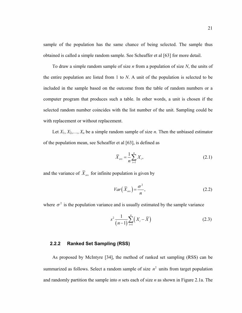
sample of the population has the same chance of being selected. The sample thus

obtained is called a simple random sample. See Scheaffer et al [63] for more detail.

To draw a simple random sample of size n from a population of size N, the units of

the entire population are listed from 1 to N. A unit of the population is selected to be

included in the sample based on the outcome from the table of random numbers or a

computer program that produces such a table. In other words, a unit is chosen if the

selected random number coincides with the list number of the unit. Sampling could be

with replacement or without replacement.

Let X1, X2,…, Xn be a simple random sample of size n. Then the unbiased estimator

of the population mean, see Scheaffer et al [63], is defined as

1

1 ,n

srs ii

X Xn =

= ∑ (2.1)

and the variance of srsX for infinite population is given by

( )2

,srsVar Xnσ

= (2.2)

where 2σ is the population variance and is usually estimated by the sample variance

( ) ( )2

1

11

n

ii

s X Xn =

−− ∑ (2.3)

2.2.2 Ranked Set Sampling (RSS)

As proposed by McIntyre [34], the method of ranked set sampling (RSS) can be

summarized as follows. Select a random sample of size 2n units from target population

and randomly partition the sample into n sets each of size n as shown in Figure 2.1a. The

22

units within each set are then ranked with respect to a variable of interest. Then the n

measurements are obtained by taking the smallest unit from the first set, second smallest

from the second set. The procedure continues in this manner until the largest unit is been

selected from nth set. The diagonal of Figure 2.1c represent our single-cycled (i.e. m = 1)

ranked set samples in this case. The cycle may be repeated m times until nm units have

been measured. Thus, the nm units form the RSS sample data.

Let ( : )i n jX denote the ith order statistic from the ith sample of size n in the jth cycle,

then the unbiased estimator for the population mean, see Takahasi and Wakimoto [76],

is defined as

( : )1 1

1 m n

rss i n jj i

X Xnm = =

= ∑∑ (2.4)

and the variance of rssX is given by

( ) 2( : )

1

1 ,n

rss i ni

Var Xnm

σ=

= ∑ (2.5)

where ( )( )( )22( : ) ( : ) ( : )i n i n i nE X E Xσ = − is the population variance of the ith order statistic.

Right from the early works of McIntyre [34], Takahasi and Wakimoto [76] and

subsequent adjustments discussed in section 1.2.2, it is noted that the variance of the

RSS mean ( )rssVar X is smaller than that of the SRS, ( )srsVar X . In other words, the

population mean estimated by the RSS mean rssX is more efficient than the one

estimated by SRS mean srsX .

23

Figure 2.1: Setup of a Ranked Set Sampling scheme.

X

Selected 2n units

X

XX XX

X X

X XX

X

XX

X

XX

X

XX

XX

X XX

XX X

X

X

X

RRaannkk wwiitthhiinn sseettss

Measure only diagonal samples

11 12 1

21 22 2

1 2

1 2

n

n

n n nn

nX X XX X X

X X X

SSeettss

(a)

(11) (12) (1 )

(21) (22) (2 )

( 1) ( 2) ( )

1 2

n

n

n n nn

nX X XX X X

X X X

RRaannkkeedd SSeettss

(b)

(11) (12) (1 )

(21) (22) (2 )

( 1) ( 2) ( )

1 2

n

n

n n nn

nX X XX X X

X X X

Ranked Sets

(c)

Randomly allocate to sets

24

2.2.3 Median Ranked Set Sampling (MRSS)

The method of median ranked set sampling (MRSS) proposed by Muttlak [42] can

be summarized as follows. Randomly select a sample of size 2n units from target

population and partition the sample into n sets each of size n and rank the units of each

set with respect to a variable of interest. The n measurements are then obtained

depending on whether the set size is even or odd. For odd set sizes, select the median

value for measurement from each ranked set (i.e. the ( )( 1) 2 thn + smallest rank). And

for the even set sizes, select the ( )2 thn smallest element from the first 2n sets and

select ( )( 2) 2 thn + smallest element from the remaining 2n sets. The cycle may be

repeated m times until nm units have been measured. Thus, the nm units form the MRSS

sample data.

Let ( : )i m jX represent the ith median from the ith set of size n in the jth cycle if the set

size is odd. Also let the same notation represent the ( )2 thn order statistic the ith set of

size n ( 1, 2, , 2)i k n= =… and the ( )( 2) 2 thn + order statistic the ith set of size n

( 1, 2, , )i k k n= + + … in the jth cycle if the set size is even. Then the estimator for the

population mean and its variance are respectively given by, see Muttlak [42]

( : )1 1

1 m n

mrss i m jj i

X Xnm = =

= ∑∑ (2.6)

( ) 2( : )

1

1 ,n

mrss i mi

Var Xnm

σ=

= ∑ (2.7)

25

where ( )( )22( : ) ( : ) ( : )i m i m i mE X E Xσ = −

is the population variance of the ith order statistic.

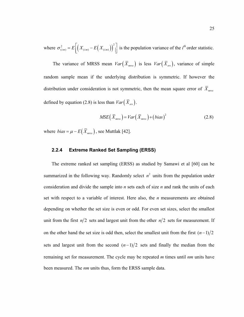
The variance of MRSS mean ( )mrssVar X is less ( )srsVar X , variance of simple

random sample mean if the underlying distribution is symmetric. If however the

distribution under consideration is not symmetric, then the mean square error of mrssX

defined by equation (2.8) is less than ( )srsVar X .

( ) ( ) ( )2mrss mrssMSE X Var X bias= + (2.8)

where ( )mrssbias E Xµ= − , see Muttlak [42].

2.2.4 Extreme Ranked Set Sampling (ERSS)

The extreme ranked set sampling (ERSS) as studied by Samawi et al [60] can be

summarized in the following way. Randomly select 2n units from the population under

consideration and divide the sample into n sets each of size n and rank the units of each

set with respect to a variable of interest. Here also, the n measurements are obtained

depending on whether the set size is even or odd. For even set sizes, select the smallest

unit from the first 2n sets and largest unit from the other 2n sets for measurement. If

on the other hand the set size is odd then, select the smallest unit from the first ( 1) 2n −

sets and largest unit from the second ( 1) 2n − sets and finally the median from the

remaining set for measurement. The cycle may be repeated m times until nm units have

been measured. The nm units thus, form the ERSS sample data.

26

Let ( : )i e jX stand for the smallest of the ith set ( 1, 2, , 2)i v n= =… and the largest of

the ith set ( 1, 2, , )i v v n= + + … of size n in the jth cycle if the set size is even. Let the

same notation also stand for the smallest of the ith set ( 1, 2, , ( 1) 2)i w n= = −… , the

largest of the ith set ( 1, 2, , )i w w n= + + … and the median of the ith set ( ( 1) 2)i n= + of

size n in the jth cycle if the set size is odd. The estimator of the population mean and its

variance, see Samawi et al [60] are given respectively by

( : )1 1

1 m n

erss i e jj i

X Xnm = =

= ∑∑ (2.9)

( ) 2( : )

1

1 ,n

erss i ei

Var Xnm

σ=

= ∑ (2.10)

where ( )( )22( : ) ( : ) ( : )i e i e i eE X E Xσ = −

.

The variance of erssX have also been shown to less than that of srsX if the

underlying distribution is symmetric. And for the case of asymmetric distribution, the

mean square error of erssX given by

( ) ( ) ( )2erss erssMSE X Var X bias= + (2.11)

where ( )erssbias E Xµ= − , is less than ( )srsVar X . See Samawi, et al [60].

2.2.5 Double Ranked Set Sampling (DRSS)

The method of double ranked set sampling (DRSS) as proposed by Al-Saleh and

Al-Kadiri [6] can be summarized as follows. Assuming the cycle is repeated only once,

i.e. m = 1, randomly select n3 elements from the target population and divide them

27

randomly into n sets each of size 2n elements as shown in Figure 2.2a. The procedure of

ranked set sampling (RSS) is then applied on each of the set to obtain the n sets of

ranked set samples of size n each, Figure 2.2b. These ranked set samples are collected

together to form n set of elements each of size n , as can be seen in Figure 2.2c. The

RSS procedure is then applied again on this set to obtain a second stage RSS. The whole

cycle may be repeated m times to yield a sample size nm . These nm units thus, form

the double ranked set samples.

Let ( : )i n jY denote the ith order statistic from the ith sample of size n of a RSS data in

the jth cycle of size m . Then the unbiased estimator of the population mean using DRSS

data based on jth cycle as proposed by Al-Saleh and Al-Kadiri [6] is given by

( : )1

1 n

drssj i n ji

Y Yn =

= ∑ ; 1, 2, .j m= … (2.12)

And the variance of drssjY is given to be

( ) 2*( : )2

1

1 n

i ndrssji

Var Yn

σ=

= ∑ (2.13)

where ( )( )22*( : ) ( : ) ( : )i n i n i nE Y E Yσ = −

is the population variance of the ith order statistic

from RSS data.

The relative precision of DRSS with respect to both simple random sampling (SRS)

as well as ranked set sampling (RSS) have been proven to be greater than or equal to one

even without increasing the sample size n , see Al-Saleh and Al-Kadiri [6]. That is

28

Figure 2.2: Setup of a Double Ranked Set Sampling scheme.

Selected 3n units

Rank within sets

Randomly allocate to sets

XX

XX XX

X X

X XX

X

XX

X

XX

X

XX

XX

X XX

XX X

X

XX

X

22nndd SSeettss

2 2 211 12 12 2 221 22 2

2 2 21 2

1 2

n

n

n n nn

nX X XX X X

X X X

(a)

1 1 111 12 11 1 121 22 2

1 1 11 2

1 2

n

n

n n nn

nX X XX X X

X X X

11sstt SSeettss

, .... ,

1 1 1(11) (12) (1 )1 1 1(21) (22) (2 )

1 1 1( 1) ( 2) ( )

1 2

n

n

n n nn

nX X XX X X

X X X

,

nntthh RRaannkkeedd SSeettss

(11) (12) (1 )

(21) (22) (2 )

( 1) ( 2) ( )

1 2n n n

nn n n

n

n n nn n nn

nX X XX X X

X X X

22nndd RRaannkkeedd SSeettss

(b)

2 2 2(11) (12) (1 )2 2 2(21) (22) (2 )

2 2 2( 1) ( 2) ( )

1 2

n

n

n n nn

nX X XX X X

X X X

11sstt RRaannkkeedd SSeettss

Measure only diagonal samples

…

,11 12 1

21 22 2

1 2

1 2n n n

nn n n

n

n n nn n nn

nX X XX X X

X X X

nntthh SSeettss

Ranked Sets (Step 2)

(c)

(2) ( )(11) (11) (11)(1) ( )(22) (22) (22)

(1) (2)( ) ( ) ( )

1 2n

n

nn nn nn

nY X XX Y X

X X Y

29

( )( )

( )( ) 1srs rss

drss drss

Var X Var XRP

Var Y Var Y= ≥ ≥ . (2.14)

Equality holds in cases where judgment ranking is poor enough to produce a simple

random sample. Ranking in the second stage to obtain DRSS data have been shown to

be much easier than ranking in the first stage which yields the RSS data. And that the

new method is cost effective and yields accurate estimator for the population mean.

2.3 Control Chart Preliminaries

The application and success of a control chart largely depends on a good sampling

method as it involves drawing of samples of fixed size n from a production process at

regular sampling intervals. The values X1, X2,…., Xn that can be observed from the

quality characteristic that is been monitored are usually summarized in the sample vector

X, which are either used in their original form or are condensed to a sample statistic such

as the sample mean, sample range or sample standard deviation.

A control chart consists of three horizontal lines as shown in Figure 2.3. The center

line (CL) represents the average value of the quality characteristics taken from a pre-run

of the manufacturing process in state of statistical control. The other two lines are called

the upper control limit (UCL) and lower control limit (LCL). The UCL and LCL are

often calculated in such a way that nearly all the sample points are between the two lines

when the process is in the state of control. Most often, the sample points on a control

chart are connected with straight lines for easy visualization of over time evolvement of

sequence of points.

30

Sample number or time

Qua

lity

char

acte

ristic

s fo

r sam

ple

Figure 2.3: A typical control chart

In applying a control chart, there are three different possible outcomes for each

sample. It is either the observed value lies within the warning limits (i.e. inner limits

usually at 2-sigma) between the warning limits and control limits or outside the control

limits. But because the use of warning limits increase risk of false alarm, see

Montgomery [36], the following decision rules are often used in real life situations.

• Rule 1: The sample points lies between the control limits

Here the manufacturing process is assumed to be in state of statistical control,

and as such, it is not necessary to take any form of action. Thus, the process is

allowed to continue as it was.

• Rule 2: The sample points lies on or outside the control limits

If this happen, it will serve as evidence that the manufacturing process is no

longer in a state of statistical control and an immediate intervention is necessary.

UCL

CL

LCL

31

In other words, investigation and corrective action is required to find an

assignable cause or causes responsible for this abnormality.

In addition to these decision rules, if the sample points are nonrandom in nature, even if

they all lie within the control limits could be an indication that the process is out of

control, see Mittag and Rinne [35].

2.3.1 Average Run Length (ARL)

The performance of a control chart can be measured using the average run length

(ARL). It is the average number of points that must be plotted before an out-of-control

signal is observed. For a classical chart, Figure 2.3, the ARL for in-control process often

denoted by ARL0 is given by

01ARLα

= (2.15)

where α is the false alarm rate (i.e. probability of type I error). For example, the ARL

for a stable in-control for a normally distributed process is expected to be approximately

370. That is, an average of 370 control points must be plotted before an out-of-control

signal is observed.

Now if there is a shift in the process, then we expect the probability of an out-of-

control signal to increase. Since, the probability of not getting an out-of-control signal if

the process has shifted is β (i.e. probability of type II error) then the probability of

getting an out-of-control signal would be 1 – β. Thus, the ARL for an out of control

process often denoted by ARL1 is given by

32

11

1ARL

β=

− (2.16)

The 1 – β is usually called the power of statistical procedure. See Alwan [1] for more

detail.

2.3.2 Variable Control Chart

Control charts can be classified into a pair of six categories, see Mittag and Rinne

[35]. Since our interest on the measurement of quality characteristic is on a numerical

scale, we make use of control chart for variables. The variable control charts are used

when the quality is measure as variables, for example, length, weight, tensile strength

etc. They have wider application in the monitoring of process mean and standard

deviation. The monitoring of the shift in process means is often carried out using the

control chart for mean X chart, X − S chart or X − R chart. While the process standard

deviation can be monitored using the S chart, or a control chart for the range, called the

R chart.

33

Chapter 3

SOME MODIFICATIONS TO DOUBLE RANKED SET SAMPLING

3.1 Introduction

In this chapter, we attempt to introduce some alternative sampling techniques to

double ranked set sampling (DRSS) method which could be much easier to apply in

practical situations. The suggested methods are median double ranked set sampling

(MDRSS), double median ranked set sampling (DMRSS) and extreme double ranked set

sampling (EDRSS).

3.2 Proposed Sampling Techniques

3.2.1 Median Double Ranked Set Sampling

In the MDRSS procedure, select n random samples each of size 2n units from the

population and apply the RSS procedure on each set to obtain n sets of ranked set

samples of size n each. The procedure of MRSS is then applied on the resultant n

samples of size n units. The whole process may be repeated m times to obtain a

measurement of nm units. These nm units obtained form a MDRSS data of size n .

34

3.2.2 Double Median Ranked Set Sampling

The procedure of double median ranked set sampling (DMRSS) can be described as

follows: Select n random samples each of size 2n units from the population and apply

the procedure of median ranked set sampling (MRSS) on each set of size n to obtain n

sets of median ranked set sampling data of n size each. The same procedure is then re-

applied on the newly formed median ranked set samples to obtain a second stage median

ranked set samples. The whole process may be repeated m times to obtain a

measurement of nm units. These nm units thus, form a double median ranked set

sampling data of size n .

3.2.3 Extreme Double Ranked Set Sampling

The procedure of EDRSS can be summarized in the following way. Draw n random

samples of size 2n units from the population under consideration. Using the procedure

of RSS on each of the set, results in n sets of ranked set samples each of size n . The

procedure for ERSS is then applied on the resultant RSS data obtained in the first stage

sampling. The cycle may be repeated m times to obtain nm elements. Thus, these nm

samples form EDRSS data

3.3 Notations and Some Definitions

Suppose that the variable of interest X has probability density function f(x), with

absolute continues distribution function F(x), mean µ and variance σ2. Let

35

1 2, , , nX X X… be a simple random sample drawn from the continuous distribution F(x).

and let assume that the ranking is perfect, so that ( : )i n jX , i = 1, 2,…., n; j = 1, 2,…., m, is

the thi order statistic in jth cycle of F(x). Then the distribution of ( : )i n jX which depends

on the rank order i but not on cycle j , has a probability distribution function (pdf) and

cumulative distribution function (cdf) given respectively by

( ) ( )1:

!( ) ( ) 1 ( ) ( )( 1)!( )!

i n ii n

nf x F x F x f xi n i

− −= −− −

, (3.1)

: :( ) ( )x

i n i nF x f y dy−∞

= ∫ . (3.2)

Let ( : )i n jY 1, 2, ,i n= … ; 1, 2, ,j m= … denotes a random variable MDRSS, DMRSS

or EDRSS samples of size n in jth cycle. Suppose that ( : )i d jY has density function

: ( )i ng x , with cumulative distribution function : ( )i nG x where

:1

( ) ( )n

i ni

g x nf x=

=∑ and :1

( ) ( )n

i ni

G x nF x=

=∑ (3.3)

then, the ( : )i d jY , 1, 2, ,i n= … ; 1, 2, ,j m= … are independent but not identically

distributed, see Al-Saleh and Al-Kadiri [6] for more detail.

3.4 Median Double Ranked Set Sampling

As the method of MDRSS involves the measurement of the elements in the middle

in step 2 sampling (i.e. step-one RSS and step-two MRSS.), it will be easy to apply in

real life situation and is prone to less error in ranking when compared to DRSS.

36

3.4.1 Efficiency of MDRSS

The efficiency of the MDRSS in estimating the population mean will be compared to

other methods discussed in Chapter 2. Let assume that the cycle is repeated only once,

i.e. 1,m = let ( )( )1 2i nY + represent the median of the thi ranked set sample ( 1,2, , )i n= …

when the set size is odd. If on the other hand the sample size is even, let ( ): 2i nY and

( )( )2 2i nY + represent the ( )2 thn and ( )( )2 2 thn + order statistic of the thi ranked set

samples ( 1, 2, , 2)i k n= =… and ( 1, 2, , )i k k n= + + … respectively.

Let srsX , and rssX be the sample means of simple random sampling (SRS) and

ranked set sampling (RSS) respectively, all with the same sample sizes. The estimators

of the population mean based on MDRSS may be defined in cases of odd and even

sample sizes respectively as

( )( )11 1 2

1 n

imdrss i n

Y Yn =

+= ∑ (3.4)

( ) ( )( )11

2 2 2 21 k

i k

n

imdrss i n i nY Y Y

n = +=+

= + ∑ ∑ (3.5)

where 2k n= . The following are properties of the above estimators

(i) If the distribution is symmetric about the population mean µ then,

( )1mdrssY µΕ = , and ( )2mdrssY µΕ = .

(ii) ( ) ( )1mdrss rssY XVar Var≤ , and ( ) ( )2Ymdrss rssXVar Var≤

(iii) If the distribution is not symmetric about the mean µ then,

37

( ) ( )1mdrss srsY XMSE Var≤ and ( ) ( )2mdrss srsY XMSE Var≤ .

Proof:

To prove (i): It is obvious that ( )1mdrssY µΕ = since the distribution is symmetric about

µ . To show the second part, we consider

( ) ( ) ( )( )1 1

2 2 221 k n

i i ki n i nmdrssY Y Y

n = = ++

Ε = Ε + ∑ ∑

( )( ) ( )( )( )1 1

2 2 21 k n

i i ki n i nY Y

n = = ++

= Ε + Ε ∑ ∑

( ) ( )( )1 1

2 2 21 k n

i i ki n i nn

µ µ= = +

+ = + ∑ ∑ (3.6)

If the distribution is symmetric about µ , then ( )2i n cµ µ= − and ( )( )2 2i n cµ µ+

= + for a

fixed constant c . Therefore ( )2mdrssY µΕ = . See Muttlak [42] and Al-Saleh and Al-

Kadiri [6].

To prove (ii), consider

( ) ( )( )( )21

1 211 n

ii nmdrssY Var Y

nVar

=+

= ∑ (3.7)

and let 1 2 1, , , , , ,md n nZ Z Z Z Z−… … be the a RSS data, with mdZ denoting its median

value. Then

( )1

1 n

irss iX Var Z

nVar

=

= ∑

( ) ( )2 21

1 1 ,n n

i i ri i rVar Z Cov Z Z

n n= ≠

= +∑ ∑

38

( ) ( )2 21

( ) ( ) ( )1 1 ,

n n

i i ri i rVar Z Cov Z Z

n n= ≠

= +∑ ∑

but ( ) ( )( ) ( )md iVar Z Var Z≤ for any i = 1, 2,…., md, .…, n-1, n, see Sinha, et al [66].

Therefore,

( ) ( ) ( )2 21

( ) ( ) ( )1 1 ,

n n

i i rmd i rrssX Var Z Cov Z Z

n nVar

= ≠

≥ +∑ ∑

( )( )( ) ( )2 21

( ) ( )1 21 1 ,

n n

i i ri ri nVar Y Cov Z Z

n n= ≠+

≥ +∑ ∑

( ) ( )2 ( ) ( )11 ,

n

i ri rmdrssY Cov Z Z

nVar

≠

≥ + ∑ (3.8)

But, ( )( ) ( ), 0i rCov Z Z ≥ . See Lehmann [33] and Essary et al [24]. Thus,

( ) ( )1mdrss rssVar Y Var X≤ (3.9)

We can similarly show that

( ) ( )2mdrss rssVar Y Var X≤ . (3.10)

To prove (iii), we consider

( ) ( ) ( )2

1 1mdrss mdrssMSE Y Var Y bias= +

( ) ( )( )2

1 1mdrss mdrssVar Y Yµ= + −Ε

( ) ( )( )2

1rss mdrssVar X Yµ≤ + −Ε (using equation 3.9)

( ) ( )( )( ) ( )( )2 2

:21

11 n

i ni

srs mdrssVar X E X E Yn

µ µ=

≤ − − + −

∑

39

But, the inequality

( )( )( ) ( )( )2 2

:21

11 n

i ni

mdrssE X E Yn

µ µ=

− ≤ −∑ (3.11)

holds for almost all the distribution if the sample size is small. This can be confirmed

from the results in Table 3.1, see Muttlak [42]. Thus,

( ) ( )1mdrss srsMSE Y Var X≤ . (3.12)

Similar argument for even case proves the second part.

3.4.2 Examples

Assume that the order statistics ( : )i nX , ( 1, 2, , )i n= … are from a distribution with pdf

f(x) and cdf F(x). Then for a sample size of n = 2, the distribution of (1:2)Y and (2:2)Y are

given respectively by, see Al-Saleh and Al-Omari [7]

( )( ) 3 4

1:2 1:2 2:2

3 42:2 1:2 2:2

( ) 1 1 ( ) 1 ( ) 2 ( ) 2 ( ) ( )

( ) ( ) ( ) 2 ( ) ( )

G x F x F x F x F x F x

G x F x F x F x F x

= − − − = − +

= = − (3.13)

The expected value and the variance of (1:2)Y and (2:2)Y , are respectively given by

( )

( )

(1:2)(1:2)

(2:2)(2:2)

( )

( )

Y xg x dx

Y xg x dx

∞

−∞

∞

−∞

Ε =

Ε =

∫

∫ (3.14)

( ) ( ){ }( ) ( ){ }

22(1:2) (1:2)

(1:2)

22(2:2) (2:2)

(2:2)

( )

( )

Var Y x g x dx Y

Var Y x g x dx Y

∞

−∞

∞

−∞

= − Ε

= − Ε

∫

∫ (3.15)

40

For n = 3, the distributions of (1:3)Y , (2:3)Y and (3:3)Y are given by

( )( )( )1:3 1:3 2:3 3:3

3 4 5 6 7 8 9

( ) 1 1 ( ) 1 ( ) 1 ( )

3 ( ) 9 ( ) 12 ( ) 9 ( ) 12 ( ) 15 ( ) 9 ( ) 2 ( )

G x F x F x F x

F x F x F x F x F x F x F x F x

= − − − −

= − + − + − + −

2:3 1:3 3:33 4 5 6 7 8 9

( ) 3 ( ) ( ) ( )

9 ( ) 12 ( ) 9 ( ) 21 ( ) 30 ( ) 18 ( ) 4 ( )

G x F x G x G x

F x F x F x F x F x F x F x

= − −

= − + − + − + (3.16)

3:3 1:3 2:3 3:3( ) ( ) ( ) ( )G x F x F x F x= 6 7 8 99 ( ) 15 ( ) 9 ( ) 2 ( )F x F x F x F x= − + −

Again the expected values and the variances of (1:3)Y , (2:3)Y and (3:3)Y , are respectively

( )

( )

( )

(1:3)(1:3)

(2:3)(2:3)

(3:3)(3:3)

( )

( )

( )

Y xg x dx

Y xg x dx

Y xg x dx

∞

−∞

∞

−∞

∞

−∞

Ε =

Ε =

Ε =

∫

∫

∫

(3.17)

( ) ( ){ }( ) ( ){ }( ) ( ){ }

22(1:3) (1:3)

(1:3)

22(2:3) (2:3)

(2:3)

22(3:3) (3:3)

(3:3)

( )

( )

( )

Var Y x g x dx Y

Var Y x g x dx Y

Var Y x g x dx Y

∞

−∞

∞

−∞

∞

−∞

= − Ε

= − Ε

= − Ε

∫

∫

∫

(3.18)

We now compute the efficiency of proposed estimators for the population mean

using MDRSS method with respect to SRS estimator given by

( ) ( ) ( ),srs mdrss srs mdrssEff X X Var X Var X= (3.19)

for three distributions namely: normal, uniform and exponential. Note that if the

underlying distribution is not symmetric, we replace ( )mdrssVar X by ( )mdrssMSE X in

equation (3.19).

41

1. Uniform Distribution, U(0,1)

Using the above relations for (1:2)Y and (2:2)Y , i.e. when n = 2 we have approximately to

five decimals, ( ) ( )(1:2) (2:2)[ , ]E Y E Y = (0.3000, 0.7000) and ( ) ( )(1:2) (2:2)[ , ]Var Y Var Y =

(0.0433, 0.0433). Thus the efficiency of MDRSS with respect to SRS is 1.9231.

For n = 3, we have

( ) ( ) ( )(1:3) (2:3) (3:3)[ , , ]E Y E Y E Y = (0.2107, 0.5000, 0.7893) and ( )(1:3)[Var Y , ( )(2:3)Var Y

( )(3:3) ]Var Y = (0.02400, 0.0346, 0.02340) and the corresponding efficiency for the

median is 2.4063.

2. Normal Distribution, N(0,1)

We have for n = 2, ( ) ( )(1:2) (2:2)[ , ]E Y E Y = (-0.6632, 0.6632) and ( )(1:2)[ ,Var Y ( )(2:2) ]Var Y

= (0.5602, 0.5602). Hence the efficiency of MDRSS with respect to SRS is 1.7852

(using numerical integration)

For n = 3, we have ( ) ( ) ( )(1:3) (2:3) (3:3)[ , , ]E Y E Y E Y = (-0.9646, 0.0000, 0.9646) and

( )(1:3)[Var Y , ( )(2:3)Var Y ( )(3:3) ]Var Y = (0.4313, 0.2767, 0.4313) and the corresponding

efficiency for median is 3.6145 (using numerical integration).

3. Exponential Distribution, Exp(1)

With the same formula, we have for n = 2, ( ) ( )(1:2) (2:2)[ , ]E Y E Y = (0.4167, 1.5833) and

( ) ( )(1:2) (2:2)[ , ]Var Y Var Y = (0.1458, 1.1736). Hence the efficiency of MDRSS with

respect to SRS is 1.5158 (using numerical integration).

42

For n = 3, we have ( ) ( ) ( )(1:3) (2:3) (3:3)[ , , ]E Y E Y E Y = (0.2599, 0.7802, 1.9599) and

( )(1:3)[Var Y , ( )(2:3)Var Y ( )(3:3) ]Var Y = (0.0521, 0.2054, 1.2250). The corresponding

efficiency for MDRSS is 2.8536. See Section 3.7 for more efficiency of MDRSS and

those of other sampling methods.

3.5 Double Median Ranked Set Sampling

This new method has to do with the measurement of the elements in the middle both

in first and second stage sampling. In other words, measure of the median of the

medians. This proposed method will be easy to apply in practical situations and will also

save time spent on ranking the units with respect to the variables of interest.

3.5.1 Efficiency of DMRSS

The efficiency of the DMRSS in estimating the population mean will be compared to

other methods discussed in Chapter 2. Let assume 1,m = and let ( )( )*

1 2i nY+

be the median

of the ith median ranked set sample (i = 1, 2, …, n) when the set size is odd. In other

words, the ( )( )1 2 thn+ order statistic of the ith order median ranked set sample denotes

DMRSS. If the set size is even, let ( )*

2i nY and ( )( )*

2 2i nY+

be the ( )2 thn and ( )( )2 2 thn +

order statistic of the ith median ranked set samples (i = 1, 2, …, k=1/n) and (i = k+1,

k+2, …, n) respectively.

The estimators of the population mean µ using DMRSS can be defined for the cases

odd and even sample sizes respectively as

43

( )( )1

*1 2 2

1 n

idmrss i n

Yn

Y=

+= ∑ (3.20)

( ) ( )( )11

* *2 2 2 2

1 k

i k

n

idmrss i n i nY Y Y

n = +=+

= + ∑ ∑ (3.21)

where k = n/2. The following properties hold for estimators given in equations (3.20)

and (3.21). If the distribution is symmetric about µ , then ( )1dmrssYΕ and ( )2dmrssYΕ are

unbiased estimators population mean µ .

(i) ( ) ( )1dmrss rssY XVar Var≤ , and ( ) ( )2dmrss rssY XVar Var≤

(ii) If the distribution is not symmetric about µ , then

( ) ( )1dmrss srsY XMSE Var≤ , and ( ) ( )2dmrss srsY XMSE Var≤

The proof of these properties follows immediately from Section 3.4.1.

3.5.2 Examples

Considering the case when n = 3, the distributions of *(1:3)Y , *

(2:3)Y and *(3:3)Y are given

respectively by

2 31:3 1:3 1:3 1:3

2 3 4 5

6 7 8 9

( ) 3 ( ) 3 ( ) ( )

9 ( ) 36 ( ) 84 ( ) 126 ( ) 126 ( )84 ( ) 36 ( ) 9 ( ) ( )

G x F x F x F x

F x F x F x F x F xF x F x F x F x

= − +

= − + − +

= − + − +

3 93:3 3:3( ) ( ) ( )G x F x F x= = . (3.22)

2 3

2:3 2:3 2:34 5 6 7 8 9

( ) 3 ( ) 2

12 ( ) 36 ( ) 42 ( ) 108 ( ) 72 ( ) 16 ( )

G x F x F

F x F x F x F x F x F x

= −

= − − + − +

44

The expected values and the variance of *(1:3)Y , *

(2:3)Y and *(3:3)Y are related to those in the

previous example. And on the computation of the efficiency of proposed estimators for

the population mean using DMRSS method with respect to SRS estimator given by

( ) ( ) ( ),srs dmrss srs dmrssEff X X Var X Var X= (3.23)

where ( )dmrssVar X is replaced by ( )dmrssMSE X for asymmetric distribution, we

consider as before three distributions: normal, uniform and exponential.

1. Uniform Distribution, U(0,1)

If we use the formula for the distributions of *(1:3)Y , *

(2:3)Y and *(3:3)Y , i.e. for the case n = 3

we have approximately the following results:

( ) ( ) ( )* * *(1:3) (2:3) (3:3)[ , , ]E Y E Y E Y = (0.1000, 0.5000, 0.9000) and ( )*

(1:3)[Var Y , ( )*(2:3)Var Y

( )*(3:3) ]Var Y = (0.0082, 0.0266, 0.0082). Measuring only the median value, the

corresponding efficiency is 3.1301. See Section 3.7 for more detail.

2. Normal Distribution, N(0,1)

For n = 3, we have

( ) ( ) ( )* * *(1:3) (2:3) (3:3)[ , , ]E Y E Y E Y = (-1.4453, 0.0000, 1.4453) and ( )*

(1:3)[Var Y , ( )*(2:3)Var Y

( )*(3:3) ]Var Y = (0.4436, 0.2003, 0.4436) and the corresponding efficiency if only the

median is measured is 4.9889.

45

3. Exponential Distribution, Exp(1)

For n = 3, we have ( ) ( ) ( )* * *(1:3) (2:3) (3:3)[ , , ]E Y E Y E Y = (0.1111, 0.7564, 2.8290) and

( )*(1:3)[Var Y , ( )*

(2:3)Var Y ( )*(3:3) ]Var Y = (0.0124, 0.1428, 1.5398). The corresponding

efficiency if only the median is measured is 3.1160. More efficiency of DMRSS is given

in Section 3.7.

3.6 Extreme Double Ranked Set Sampling

The method of EDRSS can be carried out with less error in ranking, as it is always

easy to identify the largest and the smallest elements within a sample. Performing such a

task in the second stage (i.e. step-one RSS and step-two ERSS), will considerably reduce

the amount of errors in ranking the units of the variable of interest.

3.6.1 Efficiency of EDRSS

The efficiency of EDRSS in estimating the population mean will be compared to

other methods discussed in Chapter 2. Assuming m = 1, let 2 1(1)iY − be the smallest of the

thi set of ranked set samples ( 1, 2, , 2)i n= … and 2 ( )i nY be the largest of the thi set of

ranked set samples ( 1, 2, , 2)i n= … for even set size n of samples. And for the case of odd

sample sizes, let (1)iY be the smallest of the thi set of ranked set samples

( 1) 2( 1, 2, , )ni w −= =… , ( )i nY be the largest of the thi set of ranked set samples

( 1, 2, , 1)i w nw= + −+ … , and ( )( 1) 2n nY + be the median of the thn ranked set sample.

46

If we let srsX , and rssX denotes the sample means for SRS and RSS respectively,

and from equal sample sizes, then the estimator of population mean using EDRSS can be

defined for the cases of even and odd sample sizes respectively by

1 11 2 1(1) 2 ( )

1 k k

i iedrss i i nY Y Y

n = =−

= + ∑ ∑ (3.24)

( )

1

1 12 (1) ( ) ( 1) 2

1 w n

i i wedrss i i n n nY Y Y Y

n

−

= = ++

= + + ∑ ∑ . (3.25)

where 2k n= and ( 1) 2w n= − . If the underlying distribution is symmetric about µ

then, we can easily show that 1edrssY and 2edrssY are unbiased estimators of the

population mean µ . Table 3.1 indicates that ( )1;2edrssYVar ≤ ( )rssXVar if the

underlying distribution is uniform or normal for both the odd and even cases.

3.6.2 Examples

Suppose that we have the same setup of Example 3.4.2, then we compute the

efficiencies of the EDRSS estimators for the population mean with respect to SRS

estimator i.e.

( ) ( ) ( ),srs edrss srs edrssEff X X Var X Var X= (3.26)

where ( )edrssMSE X replaces ( )edrssVar X for asymmetric distribution. The earlier three

distributions are once again considered and the summaries of the results for efficiencies

of EDRSS for 2,3, 4,5n = are given in the next section.

47

3.7 Comments on the Efficiency of Proposed Sampling Methods

The use of DRSS for the estimation of the population mean will always increase the

relative efficiency better than the RSS, see Al-Saleh and Al-Kadiri [6]. But its practical

application most especially for sample size greater then five will not be an easy task

because of the difficulty in ranking the units for the variables of interest. In other words,

it is prone to errors in ranking and this could reduce its efficiency. For these reason, we

introduce MDRSS, DMRSS and EDRSS, which will be easy to implement in the field.

The efficiencies of these new methods: MDRSS, DMRSS, EDRSS and those of

RSS, MRSS, ERSS and DRSS are given in Table 3.1 for three distributions namely:

uniform, normal and exponential. From the results in Table 3.1, we can deduce the

following:

1. If the underlying distribution is uniform, then there is a gain in the efficiency of

MDRSS, DMRSS and EDRSS estimators for different values of n. Observe that

the DMRSS and EDRSS estimators dominates the estimators for the rest of the

methods including DRSS. For example, if n = 5 the relative efficiency for

estimating the population mean using DMRSS is 6.925, EDRSS is 6.998, as

compared to 5.816 of DRSS.

2. For the case of normal distribution with mean zero and variance one, a general

increase in efficiency for the method of MDRSS, DMRSS and EDRSS is

observed. Also, the efficiency of DMRSS based estimator is twice the efficiency

48

of each of remaining methods, DRSS inclusive but except MDRSS. Example: If

n = 5, the efficiency of DMRSS is 12.226 as compared to DRSS which has

4.462.

3. If the underlying distribution is not symmetric, as in the exponential distribution,

there is a loss in the efficiency of the MDRSS, DMRSS and EDRSS estimators

as the sample size increases. The method appears not to be doing better than the

DRSS but better than SRS with MDRSS and DMRSS doing as well as RSS.

Distribution N Sampling Methods

RSS MRSS ERSS DRSS MDRSS DMRSS EDRSS

2 1.500 1.500 1.500 1.923 1.923 1.923 1.923

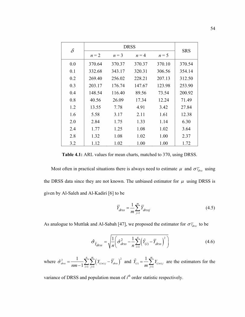
Uniform 3 2.000 1.667 2.000 3.026 2.406 3.130 3.026

U(0,1) 4 2.500 2.083 3.125 4.711 4.073 5.514 5.587

5 3.000 2.333 3.621 5.816 4.352 6.925 6.998

2 1.467 1.467 1.467 1.785 1.785 1.785 1.785

Normal 3 1.914 2.229 1.787 2.633 3.615 4.992 2.633

N(0,1) 4 2.347 2.774 2.034 3.526 5.045 7.632 2.710

5 2.770 3.486 2.234 4.462 7.323 12.226 3.421

2 1.333 1.333 1.333 1.516 1.516 1.516 1.923

Exponential 3 1.636 2.250 1.636 2.024 2.854 3.116 2.024

Exp(1) 4 1.920 2.441 1.170 2.374 2.601 4.824 1.225

5 2.190 2.230 1.444 3.375 2.189 2.226 1.601

Table 3.1: Relative efficiency for three distributions, for estimating the population mean

using RSS, MRSS, ERSS, DRSS, MDRSS, DMRSS and EDRSS methods.

49

Chapter 4

CONTROL CHART FOR MONITORING THE PROCESS MEAN

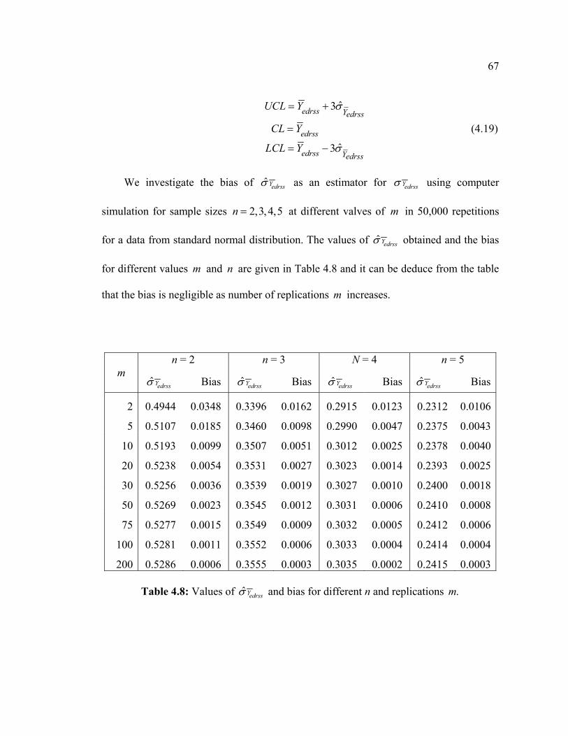
4.1 Introduction

In this chapter, an attempt is made to develop control charts based on double ranked

set sampling and its suggested modifications for monitoring a process to detect changes

in the mean. The average run length (ARL) performance of these charts will be

investigated and compared to the traditional control charts for the mean using simple

random sampling (SRS) and other sampling techniques.

4.2 Shift in Process Mean

The average run length (ARL) assumes that the process is in the state of statistical

control with mean 0µ and standard deviation 0σ , and at certain point in time the process

start to get out of statistical control with a shift in mean from 0µ to 1 0 0 nµ µ δσ= + ,

Figure 4.1, see Montgomery [36] for more detail. Now, assuming that the process

follows a normal distribution with mean 0µ and variance 20σ when the process is in the

state of statistical control, the shift on the process mean is given by 1 0 0nδ µ µ σ= − .

Note that if a point is outside the control limits when the process is in state of control

i.e. 0δ = , then it is a false alarm.

50

Figure 4.1: Shift in process mean from 0µ to 1 0 0 nµ µ δσ= +

4.3 Control Chart for Mean using SRS

Considering the Shewhart [65] control chart for mean using SRS, let Xij for i = 1,

2,…, n and j = 1, 2,…., m denote the m samples each of size n and from a normal

distribution with mean µ and variance σ2. If both the population mean µ and variance

2σ are known, then the sample mean is given by

1

1 n

j iji

X Xn =

= ∑ ; 1, 2, ,j m= … (4.1)

can be plotted on the chart for mean

3

3

UCLn

CL

LCLn

σµ

µσµ

= +

=

= −

(4.2)

where UCL, CL and LCL are the upper central limit, central limit and lower central limit

respectively. The average run length (ARL) for this chart is as described in Section 2.3.1

of Chapter 2, see Salazar and Sinha [59].

UCL LCLµ0 µ1

σ0

51

4.4 Control Chart for Mean using RSS, MRSS or ERSS

The RSS, MRSS or ERSS mean of the thj cycle denoted by ,ssjX can be plotted on

the control chart for mean based on their respective data as suggested by Muttlak and

Al-Sabah [47], and Salazar and Sinha [59] as follows

3

3

X

X

ss

ss

UCL

CLLCL

µ σ

µµ σ

= +

== −

(4.3)

where 1

2 2( : )(1 )

n

ii nXss

n σσ=

= ∑ with the values of 2( : )i nσ being obtained from the table of

order statistics for the standard normal distribution, see for example Harter and

Balakrishnan [26].

4.5 Control Chart for Mean using DRSS

Let the drssjY represent the mean of the thj cycle of DRSS we want to plot on the

control chart for mean based on DRSS data. Assuming the process is following the

normal distribution 2( , ),N µ σ with a known variance 2( : )i nσ of thi order statistic for RSS

then, the control chart based on DRSS data are given by

3

3

Ydrss

Ydrss

UCL

CLLCL

µ σ

µµ σ

= +

== −

(4.4)

52

UCL

LCL

CL

where 1

22 *( : )(1 )

n

i

i nYdrssn σσ

=

= ∑ and ( )( )22*( : ) ( : ) ( : )i n i n i nE Y E Yσ = −

is the variance for ith

order statistic using DRSS method which is calculated using numerical integration.

4.5.1 Visual Comparison of DRSS with SRS for Mean Chart

Assuming that ijX 1, 2, ,i n= … ; 1, 2, ,j m= … are from stable normal distribution

with mean µ and variance 2σ . Using a sample of size 3n = with a run length of

50m = , a simulation for the above process with 0µ = and 2 1σ = was carried out for

the SRS (Figure 4.2) based control chart for means. The means of DRSS data was also

plotted on the same chart to see their pattern. Figure 4.2 indicates that the means

estimated by DRSS have less variability as compared to those estimated by SRS.

-2.0

-1.5

-1.0

-0.5

0.0

0.5

1.0

1.5

2.0

1 4 7 10 13 16 19 22 25 28 31 34 37 40 43 46 49Observations

Mea

ns

SRS DRSS

Figure 4.2: Control chart for mean using SRS & DRSS for same process.

53

4.5.2 ARL Comparison of DRSS with other Mean Chart

In support of our visual comparison that the control charts based on DRSS has less

variability than the classical SRS chart, we make use of the average run length (ARL).

As with the works of Muttlak and Al-Sabah [47] and Salazar and Sinha [59], we

considered only simulation for the first rule (a point out of control limits) and for each

shift, 1,000,000 iterations were simulated. The control limits, equation (4.4), of the

DRSS based control chart for means are computed using numerical integration.

Considering only the case for perfect ranking i.e. when ranking the variable of

interest without error in ranking the units, we run computer simulations for various

values of δ , 0.0,0.1,0.2,0.3,0.4,0.8,1.2,1.6,2.0,2.4, 3.2.andδ = , when the sample sizes

are 2,3, 4,5n = . For a better comparison of the performance of DRSS with SRS, it is

advisable to match the ARL to the accepted false alarm rate in the traditional SRS chart,

ARL0 = 370.40. See Champ & Woodall [14], and Salazar & Sinha [59] for a detail.

Hence, we open the control limits up to 3.072 Ydrssσ and the results are displayed in

Table 4.1. The ARL values for the classical SRS chart reported in Table 4.1 are

independent of the sample size. See Champ & Woodall [14]. Also, the simulation results

based on the usual 3 Ydrssσ are presented in section 4.9.

Table 4.1 indicates that the new charts based on DRSS gives better ARL

performance as compared to the SRS. Observe that for 2n ≥ and 1.2 2.4δ≤ ≤ the ARL

value of DRSS are less than half the corresponding values for the SRS and is even less

than one-quarter of the corresponding values of SRS when 5n ≥ and 0.8 2.0δ≤ ≤ .

54

DRSS δ

n = 2 n = 3 n = 4 n = 5 SRS

0.0 370.64 370.37 370.37 370.10 370.54 0.1 332.68 343.17 320.31 306.56 354.14 0.2 269.40 256.02 228.21 207.13 312.50 0.3 203.17 176.74 147.67 123.98 253.90 0.4 148.54 116.40 89.56 73.54 200.92 0.8 40.56 26.09 17.34 12.24 71.49 1.2 13.55 7.78 4.91 3.42 27.84 1.6 5.58 3.17 2.11 1.61 12.38 2.0 2.84 1.75 1.33 1.14 6.30 2.4 1.77 1.25 1.08 1.02 3.64 2.8 1.32 1.08 1.02 1.00 2.37 3.2 1.12 1.02 1.00 1.00 1.72

Table 4.1: ARL values for mean charts, matched to 370, using DRSS.

Most often in practical situations there is always need to estimate µ and drssYσ using

the DRSS data since they are not known. The unbiased estimator for µ using DRSS is

given by Al-Saleh and Al-Kadiri [6] to be

1

1 m

jdrss drssjY Y

m =

= ∑ (4.5)

As analogue to Muttlak and Al-Sabah [47], we proposed the estimator for drssYσ to be

( )2

1

2( )

1 1ˆˆn

idrss i drssYdrss

Y Yn n

σσ=

= − −

∑ (4.6)

where ( )22( : )

1 1

1ˆ1

n m

drss i n j drssi j

Y Ynm

σ= =

= −− ∑∑ and ( ) ( : )

1

1 m

i i n jj

Y Ym =

= ∑ are the estimators for the

variance of DRSS and population mean of ith order statistic respectively.

55

Our control charts may now be constructed based on drssY and ˆ drssYσ as follows:

ˆ3

ˆ3

drss

drss

Y

Y

drss

drss

drss

UCL Y

CL Y

LCL Y

σ

σ

= +

=

= −

(4.7)

Clearly, the proposed estimator ( ˆ drssYσ ) is biased estimator for drssYσ , and hence a

need to investigate the level of its biasness. We employ computer simulation in this

direction. Simulations were carried out using data from standard normal distribution for

sample sizes 2,3,4,5n = at different values of m using 50,000 iterations. The values of

ˆ drssYσ obtained together with the bias are tabulated in Table 4.2 and from the table, we

can see that the bias become very small as number of replications m increases.

n = 2 n = 3 n = 4 n = 5 m ˆ drssYσ Bias ˆ drssYσ Bias ˆ drssYσ Bias ˆ drssYσ Bias

2 0.4944 0.0348 0.3396 0.0162 0.2564 0.0098 0.2053 0.0064

5 0.5107 0.0185 0.3460 0.0098 0.2600 0.0061 0.2074 0.0042

10 0.5193 0.0099 0.3507 0.0051 0.2627 0.0034 0.2096 0.0020

20 0.5238 0.0054 0.3531 0.0027 0.2644 0.0018 0.2108 0.0008

30 0.5256 0.0036 0.3539 0.0019 0.2650 0.0012 0.2112 0.0005

50 0.5269 0.0023 0.3545 0.0012 0.2655 0.0007 0.2114 0.0002

75 0.5277 0.0015 0.3549 0.0009 0.2657 0.0004 0.2115 0.0001

100 0.5281 0.0011 0.3552 0.0006 0.2659 0.0002 0.2117 0.0000

200 0.5286 0.0006 0.3555 0.0003 0.2661 0.0001 0.2118 0.0001

Table 4.2: Values of ˆ drssYσ and bias for different n and replications .m

56

4.6 Control Chart for Mean using MDRSS

Assuming the process is following a normal distribution 2( , ),N µ σ with a known

variance. Then the MDRSS mean of the thj cycle denoted by mdrssjY can be plotted on

the following control chart for mean based on MDRSS data

3

3

Ymdrss

Ymdrss

UCL

CLLCL

µ σ

µµ σ

= +

== −

(4.8)

where 1

2 2( : )(1 )

n

ii mdYmdrss

n σσ=

= ∑ and ( )( )22( : ) ( : ) ( : )i md i md i mdE Y E Yσ = −

is the thi

variance for MDRSS calculated using numerical integration.

4.6.1 Visual Comparison of MDRSS with SRS for Mean Chart

Assume that the MDRSS data are from normal distribution with mean µ and

variance 2σ . Using a sample of size 3n = with a run length of 50m = , we simulate the

above process with 0µ = and 2 1σ = for the SRS based mean chart, Figure 4.3. We also

plot the means of MDRSS data on same chart to see how much two charts vary. From

Figure 4.3 we observe that the mean estimated by MDRSS have less variability as

compared to those estimated using SRS.

4.6.2 ARL Comparison of MDRSS with other Mean Chart

Again, considering simulation for a point out of control limits only, we carried out

simulations for various values of δ (as in Section 4.5.2) in 1,000,000 iterations.

57

UCL

CL

LCL

-2.0

-1.5

-1.0

-0.5

0.0

0.5

1.0

1.5

2.0

1 3 5 7 9 11 13 15 17 19 21 23 25 27 29 31 33 35 37 39 41 43 45 47 49Observations

Mea

nsSRS MDRSS

Figure 4.3: Control chart for mean using SRS & MDRSS for same process.

The control limits of the MDRSS based chart for the mean in equation 4.8 are computed

using numerical integration. Here again, we considered only the case for perfect ranking

and run computer simulations for various values of δ, when the sample size are n = 2, 3,

4 and 5. The control limits were open up to 3.021 mdrssYσ to match the ARL to the

accepted false alarm rate in the classical SRS chart, and the results are in Table 4.3.

From Table 4.3 we can see that the ARL performance of new charts based on

MDRSS are better as compared to the SRS method. Also from the table, we see that the

ARL values of MDRSS are less than half the corresponding values for the SRS when

3n ≥ and 0.4 2.8δ≤ ≤ while for 5n ≥ and 0.4 2.0δ≤ ≤ the ARL values of MDRSS is

one-fifth less than those of the corresponding SRS.

58

MDRSS δ n = 2 n = 3 n = 4 n = 5

SRS

0.0 370.10 370.37 370.64 370.64 370.54 0.1 332.67 317.66 297.80 267.52 354.14 0.2 269.25 217.01 184.84 143.18 312.50 0.3 203.00 130.51 100.77 69.46 253.90 0.4 148.46 81.87 57.71 36.06 200.92 0.8 40.55 15.01 9.03 5.01 71.49 1.2 13.55 4.37 2.69 1.68 27.84 1.6 5.58 1.96 1.39 1.10 12.38 2.0 2.84 1.28 1.08 1.01 6.30 2.4 1.77 1.06 1.01 1.00 3.64 2.8 1.32 1.01 1.00 1.00 2.37 3.2 1.12 1.00 1.00 1.00 1.72

Table 4.3: ARL values for mean chart, matched to 370, using MDRSS.

In practical situations, we need to estimate the µ and mdrssYσ using the MDRSS data

since we do not know them. But since the underlying distribution is normal, then from

chapter 3 we see that the unbiased estimator for µ using MDRSS is given by

1

1 m

jmdrss mdrssjY Y

m =

= ∑ (4.9)

We proposed the estimator for mdrssYσ to be

( )2

1 1( : )

1( 1)

ˆm n

j ii md j mdrssYmdrss

Y Yn n

σ= =

= − −

∑∑ (4.10)

where ( : )i md jY denotes the jth observation of the ith median of a RSS of size n if the set

size is odd or the (n/2)th and ((n+1)/2)th order statistic of the ith set (i = 1, 2,…,k = n/2)

59

and (I = k+1, k+2,…,n) of RSS respectively if the sample size is even. We use mdrssY and

ˆ mdrssYσ to construct the control charts as follows

ˆ3

ˆ3

mdrss

mdrss

Y

Y

mdrss

mdrss

mdrss

UCL Y

CL Y

LCL Y

σ

σ

= +

=

= −

(4.11)

We used computer simulation to investigate the level of biasness of ˆ mdrssYσ .

Simulations were carried out for a data from standard normal distribution for sample

sizes 2,3, 4,5n = at different valves of m using 50,000 iterations. The values of ˆ mdrssYσ

obtained as well as the bias are given in Table 4.4 and we can see that the bias is

negligible for any value of set size n which become very clear with the increase in

number of replications m.

n = 2 n = 3 n = 4 n = 5 m ˆ mdrssYσ Bias ˆ mdrssYσ Bias ˆ mdrssYσ Bias ˆ mdrssYσ Bias

2 0.4944 0.0348 0.2884 0.0153 0.2147 0.0079 0.1607 0.0046

5 0.5107 0.0185 0.2977 0.0060 0.2196 0.0030 0.1637 0.0015

10 0.5193 0.0099 0.3008 0.0029 0.2213 0.0013 0.1644 0.0009

20 0.5238 0.0054 0.3023 0.0014 0.2220 0.0006 0.1649 0.0003

30 0.5256 0.0036 0.3028 0.0009 0.2223 0.0003 0.1651 0.0002

50 0.5269 0.0023 0.3031 0.0006 0.2223 0.0003 0.1652 0.0001

75 0.5277 0.0015 0.3034 0.0003 0.2224 0.0002 0.1652 0.0001

100 0.5281 0.0011 0.3035 0.0002 0.2225 0.0001 0.1652 0.0000

200 0.5286 0.0006 0.3036 0.0001 0.2226 0.0000 0.1653 0.0000

Table 4.4: Values of ˆ mdrssYσ and bias for different n and replications .m

60

4.7 Control Chart for Mean using DMRSS

We assume that the process follows a normal distribution with mean µ and variance

2σ . Suppose that the variance is known then, the DMRSS mean of the jth cycle denoted

by dmrssjY can be plotted on the control chart based on DMRSS data as follows

3

3

Ydmrss

Ydmrss

UCL

CLLCL

µ σ

µµ σ

= +

== −

(4.12)

where 1

2 2( : )(1 )

n

idmrssY i dmn σσ

=

= ∑ and ( )( )22( : ) ( : ) ( : )i dm i dm i dmE Y E Yσ = −

is the variance for

thi order statistic using DMRSS method obtained using numerical integration.

4.7.1 Visual Comparison of DMRSS with SRS for Mean Chart

We assume that the DMRSS data are from 2( , )N µ σ and using same values of n,

m, in previous section, we simulate the SRS mean chart for above process with µ = 0

and 2 1σ = , and also plot the means of DMRSS data on the same chart to see their

variability, Figure 4.4. We see from Figure 4.4 that the means estimated using DMRSS

have less variability as compared to those estimated by SRS which means that they may

detect shift in process mean faster as compared to SRS.

4.7.2 ARL Comparison of DMRSS with other Mean Chart

We run computer simulations for various values of δ, n in 1,000,000 repetitions

considering only when a point is out of control limits. The control limits of the DMRSS

61

UCL

CL

LCL

-2.0

-1.5

-1.0

-0.5

0.0

0.5

1.0

1.5

2.0

1 4 7 10 13 16 19 22 25 28 31 34 37 40 43 46 49Observations

Mea

nsSRS DMRSS

Figure 4.4: Control chart for mean using SRS & DMRSS for same process.

based control chart for means in equation 4.12 is computed using numerical integration

with perfect ranking. We again open the control limits up to 3.017 dmrssYσ to match the

ARL to the accepted false alarm rate in the classical SRS chart, ARL = 370.40, and the

results are supplied in Table 4.5.

Table 4.5 suggests that the ARL performance of the DMRSS based charts have less

variability as compared to the one based on traditional SRS. Table 4.5 also shows that

the ARL values of DMRSS are less than one-third the corresponding values for the SRS

when 3n ≥ and 0.4 2.4δ≤ ≤ while for 5n ≥ and 0.4 2.0δ≤ ≤ the ARL values of

DMRSS is one-sixth less than those of the corresponding SRS.

62

DMRSS δ n = 2 n = 3 n = 4 n = 5

SRS

0.0 370.64 370.10 370.64 370.93 370.54 0.1 332.67 293.08 288.85 221.53 354.14 0.2 269.40 188.04 147.67 92.99 312.50 0.3 203.17 101.81 74.27 39.18 253.90 0.4 148.54 58.17 39.40 18.24 200.92 0.8 40.56 9.13 5.37 2.38 71.49 1.2 13.55 2.72 1.76 1.13 27.84 1.6 5.58 1.40 1.12 1.00 12.38 2.0 2.84 1.08 1.01 1.00 6.30 2.4 1.77 1.01 1.00 1.00 3.64 2.8 1.32 1.00 1.00 1.00 2.37 3.2 1.12 1.00 1.00 1.00 1.72

Table 4.5: ARL values for mean chart, matched to 370, using DMRSS.

The values of µ and dmrssYσ are usually unknown when dealing with real life

situations, so we estimate them using the DMRSS data. From chapter 3, we see that the

unbiased estimator for µ using DMRSS is

1

1 m

jdmrss dmrssjY Y

m =

= ∑ (4.13)

We proposed the estimator for dmrssYσ to be

( )2

1 1( : )

1( 1)

ˆm n

j ii dm j dmrssYdmrss

Y Yn n

σ= =

= − −

∑∑ (4.14)

where ( : )i dm jY is the jth observation of the ith median of a MRSS of size n if the set size is

odd or the (n/2)th and ((n+1)/2)th order statistic of the ith set (i = 1, 2,…,k = n/2) and (i =

63

k+1, k+2,…,n) of MRSS respectively if the sample size is even. We can now construct

our control charts using dmrssY and ˆ dmrssYσ as follows

3

3

ˆ

ˆ

dmrss

dmrss

Y

Y

dmrss

dmrss

dmrss

UCL Y

CL Y

LCL Y

σ

σ

= +

=

= −

(4.15)

The bias of ˆ dmrssYσ as an estimator for dmrssYσ was investigated using computer

simulation for sample sizes 2,3,4,5n = at different valves of m using 50,000 iterations

for a data from standard normal distribution. The values of ˆ dmrssYσ obtained and the bias

for different values of m and n are given in Table 4.6. It is clear from the table that the

bias of ˆ dmrssYσ becomes very negligible for any value of n and with increase in number

of replications m.

n = 2 n = 3 n = 4 n = 5 m ˆ dmrssYσ Bias ˆ dmrssYσ Bias ˆ dmrssYσ Bias ˆ dmrssYσ Bias

2 0.4944 0.0348 0.2464 0.0120 0.1741 0.0069 0.1242 0.0037

5 0.5107 0.0185 0.2537 0.0047 0.1784 0.0025 0.1266 0.0013

10 0.5193 0.0099 0.2561 0.0023 0.1798 0.0012 0.1271 0.0008

20 0.5238 0.0054 0.2573 0.0011 0.1806 0.0004 0.1276 0.0003

30 0.5256 0.0036 0.2577 0.0007 0.1807 0.0003 0.1277 0.0002

50 0.5269 0.0023 0.2579 0.0005 0.1808 0.0002 0.1278 0.0001

75 0.5277 0.0015 0.2582 0.0002 0.1809 0.0001 0.1278 0.0001

100 0.5281 0.0011 0.2583 0.0001 0.1809 0.0001 0.1279 0.0000

200 0.5286 0.0006 0.2584 0.0000 0.1810 0.0000 0.1279 0.0000

Table 4.6: Values of ˆ dmrssYσ and bias for different n and replications .m

64

4.8 Control Chart for Mean using EDRSS

Suppose that the process we are considering is following a normal distribution with

mean µ and variance σ2 and that the variance is known. Then, the EDRSS mean of the

thj observation edrssjY can be plotted on the control chart based on EDRSS as follows

3

3

Yedrss

Yedrss

UCL

CLLCL

µ σ

µµ σ

= +

== −

(4.16)

where 1

2 2( : )(1 )

n

ii edYedrss

n σσ=

= ∑ and ( )( )22( : ) ( : ) ( : )i ed i ed i edE Y E Yσ = −

is the thi variance

for EDRSS.

4.8.1 Visual Comparison of EDRSS with SRS for Mean Chart

Using data from the standard normal distribution (0,1)N , a computer simulation

was performed for a sample of size 4n = with forty replications for the SRS, Figure 4.5,

using control chart for means. The means of EDRSS data are also graphed within the

same chart to see the two patterns. Figure 4.5 shows that the means estimated using

EDRSS have less variability as compared to those estimated using SRS.

4.8.2 ARL Comparison of EDRSS with other Chart

As in previous sections, computer simulations were carried out for the same values

of δ, and n in 1,000,000 repetitions considering only when a point is out of control

65

UCL

CL

LCL

limits. Control limits of EDRSS based control chart for means in equation 4.16 is

calculated using numerical integration considering only perfect ranking.

-2.0

-1.5

-1.0

-0.5

0.0

0.5

1.0

1.5

2.0

1 3 5 7 9 11 13 15 17 19 21 23 25 27 29 31 33 35 37 39Observations

Mea

ns

SRS EDRSS

Figure 4.5: Control chart for mean using SRS & EDRSS for same process.

The limits were open up to 3.082 edrssYσ to give approximately the in-control ARL value

of SRS control chart for mean and results are tabulated in Table 4.7.

Considering the results in Table 4.7, it can be observed that the EDRSS based

control charts have smaller ARL values as than those based on usual SRS. We can also

see that for 3n ≥ and 0.8 2.8δ≤ ≤ the ARL values of EDRSS are less than half of the

corresponding values for the SRS and that when 5n ≥ and 0.8 2.4δ≤ ≤ , the ARL

values of EDRSS is one-third less than those of the corresponding SRS.

66

n δ

2 3 4 5 SRS

0.0 370.64 370.37 370.40 370.37 370.54 0.1 332.68 343.17 340.46 329.38 354.14 0.2 269.40 256.02 248.38 239.69 312.50 0.3 203.17 176.74 168.40 156.35 253.90 0.4 148.54 116.39 107.09 94.80 200.92 0.8 40.56 26.09 23.72 18.62 71.49 1.2 13.55 7.78 6.51 5.20 27.84 1.6 5.58 3.17 3.05 2.22 12.38 2.0 2.84 1.75 1.71 1.36 6.30 2.4 1.77 1.25 1.23 1.10 3.64 2.8 1.32 1.08 1.07 1.02 2.37 3.2 1.12 1.02 1.02 1.00 1.72

Table 4.7: ARL values for mean chart, matched to 370, using EDRSS.

The values of µ and edrssYσ are usually unknown in real life situations, we estimate

them using the EDRSS data. The unbiased estimator for µ using EDRSS is given by

1

1 m

jedrss edrssjY Y

m =

= ∑ (4.17)

We proposed the estimator for edrssYσ to be

( )2

1 1( : )

1( 1)

ˆm n

j ii ed j edrssYedrss

Y Yn n

σ= =

= − −

∑∑ (4.18)

where ( : )i ed jY is the thj observation of the EDRSS data for both the odd and even cases.

Using edrssY and ˆ edrssYσ the control charts based on EDRSS now becomes

67

ˆ3

ˆ3

edrss Yedrss

edrss

edrss Yedrss

UCL Y

CL Y

LCL Y

σ

σ

= +

=

= −

(4.19)

We investigate the bias of ˆ edrssYσ as an estimator for edrssYσ using computer

simulation for sample sizes 2,3,4,5n = at different valves of m in 50,000 repetitions

for a data from standard normal distribution. The values of ˆ edrssYσ obtained and the bias

for different values m and n are given in Table 4.8 and it can be deduce from the table

that the bias is negligible as number of replications m increases.

n = 2 n = 3 N = 4 n = 5 m

ˆ edrssYσ Bias ˆ edrssYσ Bias ˆ edrssYσ Bias ˆ edrssYσ Bias

2 0.4944 0.0348 0.3396 0.0162 0.2915 0.0123 0.2312 0.0106

5 0.5107 0.0185 0.3460 0.0098 0.2990 0.0047 0.2375 0.0043

10 0.5193 0.0099 0.3507 0.0051 0.3012 0.0025 0.2378 0.0040

20 0.5238 0.0054 0.3531 0.0027 0.3023 0.0014 0.2393 0.0025

30 0.5256 0.0036 0.3539 0.0019 0.3027 0.0010 0.2400 0.0018

50 0.5269 0.0023 0.3545 0.0012 0.3031 0.0006 0.2410 0.0008

75 0.5277 0.0015 0.3549 0.0009 0.3032 0.0005 0.2412 0.0006

100 0.5281 0.0011 0.3552 0.0006 0.3033 0.0004 0.2414 0.0004

200 0.5286 0.0006 0.3555 0.0003 0.3035 0.0002 0.2415 0.0003

Table 4.8: Values of ˆ edrssYσ and bias for different n and replications .m

68

4.9 Comparing the New Charts Based on the Standard 3-Sigma

In order to compare the new charts with SRS and RSS based on the standard 3σ ,

simulations were carried for various values of δ and n in 1,000,000 replications for the

rule: a point out of control limits, see Salazer and Sinha [59]. Using numerical

integration, the control limits for DRSS, MDRSS and DMRSS based control charts for

mean were computed. The average run length (ARL) for the SRS, RSS, MRSS and the

new methods using the standard 3σ are given in Tables 4.9 – 4.12. And from the table,

we can draw the following conclusions:

1. The ARL performance of the new charts based on DRSS, MDRSS, DMRSS and

EDRSS are generally better as compared with those based on SRS, RSS, MRSS

and ERSS even without increase in sample size n.

2. As the sample size n increases and the process starts to go out of control (i.e. δ ≥

0), the ARL performance of EDRSS appears to be just as good as the

corresponding values of MRSS but still dominates SRS, RSS and ERSS. For

example, if n = 5 and δ =0.4, the ARL values of EDRSS is 77.95 as compared to

81.58 of MRSS, 98.45 of RSS, 112.41 of ERSS and 200.01 of SRS.

3. Among the new charts, EDRSS appears to be the least in terms of ARL

performance as n increases and δ ≥ 0. It is followed by DRSS and then MDRSS

with DMRSS dominating all the charts. For example, if n = 4 and δ = 0.4, the

ARL value of DMRSS is 29.42 as compared to 55.56 of MDRSS, 76.59 of

DRSS and 94.70 of EDRSS.

69

4. Although, the new charts have proven to be better than the SRS, RSS, MRSS,

and ERSS. There is great price to pay as they all increase the false alarm rate

when a process is in a state of statistical control (i.e. δ = 0). But as the sample

size increase, the ARL value of DMRSS seems to be matching up with the

accepted false alarm rate in the traditional SRS chart for mean (i.e. ARL =

370.40). For example, if n = 5 and δ = 0, the ARL value of DMRSS is 369.34.

Sampling Methods δ SRS RSS MRSS ERSS DRSS MDRSS DMRSS EDRSS

0.0 371.55 348.43 348.43 348.43 322.79 322.79 322.79 322.79 0.1 355.31 318.37 318.37 318.37 285.21 285.21 285.21 285.21 0.2 308.12 278.67 278.67 278.67 234.49 234.49 234.49 234.49 0.3 251.86 208.31 208.31 208.31 178.01 178.01 178.01 178.01 0.4 200.40 155.27 155.27 155.27 130.10 130.10 130.10 130.10 0.8 72.03 46.96 46.96 46.96 36.69 36.69 36.69 36.69 1.2 27.79 16.44 16.44 16.44 12.43 12.43 12.43 12.43 1.6 12.38 6.98 6.98 6.98 5.21 5.21 5.21 5.21 2.0 6.31 3.56 3.56 3.56 2.70 2.70 2.70 2.70 2.4 3.64 2.16 2.16 2.16 1.72 1.72 1.72 1.72 2.8 2.37 1.53 1.53 1.53 1.29 1.29 1.29 1.29 3.2 1.72 1.23 1.23 1.23 1.11 1.11 1.11 1.11

Table 4.9: ARL values when n = 2 using different sampling techniques.

70

Sampling Methods δ SRS RSS MRSS ERSS DRSS MDRSS DMRSS EDRSS

0.0 370.54 343.20 361.56 343.06 301.15 351.00 355.08 300.84 0.1 354.14 326.80 326.80 316.14 271.89 287.84 285.05 272.32 0.2 312.50 251.37 251.37 249.85 206.99 203.28 173.50 207.58 0.3 253.90 175.48 175.48 184.70 144.55 126.29 98.37 152.02 0.4 200.92 130.87 118.89 135.87 98.47 78.06 56.50 99.77 0.8 71.49 34.09 28.15 34.09 22.52 14.42 8.91 22.94 1.2 27.84 11.14 8.83 11.14 6.93 4.25 2.61 7.01 1.6 12.38 4.65 3.70 4.65 2.98 1.93 1.39 2.99 2.0 6.30 2.45 2.02 2.45 1.67 1.27 1.08 1.70 2.4 3.64 1.60 1.39 1.60 1.22 1.06 1.01 1.23 2.8 2.37 1.23 1.13 1.23 1.06 1.01 1.00 1.07 3.2 1.72 1.08 1.04 1.08 1.02 1.00 1.00 1.02

Table 4.10: ARL values when n = 3 using different sampling techniques

Sampling Methods δ

SRS RSS MRSS ERSS DRSS MDRSS DMRSS EDRSS0.0 368.22 337.50 361.08 340.37 301.50 352.67 356.95 294.99 0.1 356.57 310.52 321.92 311.92 259.05 282.69 283.83 265.91 0.2 314.34 234.63 230.22 243.55 185.03 171.91 103.40 201.54 0.3 252.13 166.55 152.74 177.44 120.03 97.09 54.09 140.36 0.4 199.88 112.80 99.99 123.95 76.59 55.56 29.42 94.70 0.8 71.92 26.38 20.94 31.44 15.03 8.75 4.49 21.65 1.2 28.01 8.17 6.33 10.17 4.43 2.63 1.61 6.63 1.6 12.41 3.44 2.71 4.23 1.99 1.38 1.09 2.82 2.0 6.29 1.90 1.59 2.27 1.29 1.07 1.01 1.60 2.4 3.64 1.33 1.19 1.51 1.07 1.01 1.00 1.20 2.8 2.38 1.11 1.05 1.19 1.01 1.00 1.00 1.06 3.2 1.73 1.03 1.01 1.06 1.00 1.00 1.00 1.01

Table 4.11: ARL values when n = 4 using different sampling techniques

71

Sampling Methods δ SRS RSS MRSS ERSS DRSS MDRSS DMRSS EDRSS

0.0 369.04 347.11 365.44 338.07 297.42 363.41 369.34 292.47 0.1 353.23 300.66 310.06 304.05 248.45 263.98 221.17 255.51 0.2 303.58 226.96 209.79 232.75 166.07 138.55 91.61 183.81 0.3 257.50 153.63 132.34 162.41 100.89 69.04 38.99 121.83 0.4 200.01 98.45 81.58 112.41 61.08 36.12 18.31 77.95 0.8 70.58 21.02 15.16 25.06 10.63 4.96 2.38 15.69 1.2 27.91 6.35 4.47 7.82 3.13 1.67 1.13 4.66 1.6 12.37 2.72 2.02 3.32 1.54 1.10 1.00 2.07 2.0 6.30 1.59 1.30 1.85 1.12 1.01 1.00 1.31 2.4 3.65 1.19 1.07 1.30 1.02 1.00 1.00 1.08 2.8 2.37 1.05 1.01 1.10 1.00 1.00 1.00 1.02 3.2 1.72 1.01 1.00 1.03 1.00 1.00 1.00 1.00

Table 4.12: ARL values when n = 5 using different sampling techniques

72

Chapter 5

CONTROL CHART FOR MONITORING THE PROCESS MEAN AND STANDARD DEVIATION

5.1 Introduction

In this chapter, we construct control charts based on some modifications of ranked

set sampling for monitoring a process to detect shifts in mean and standard deviation.

We will also investigate the average run length (ARL) performance of these charts and

compare them with the corresponding control charts using simple random sampling

(SRS) and other sampling techniques.

5.2 Control Chart for Monitoring the Process Standard Deviation

The average run length (ARL) assumes that the process is in the state of statistical

control with mean 0µ and standard deviation 0σ . But at certain point in time, the

process begin to go out of statistical control with a shift in standard deviation from 0σ to

1 0σ σ≥ , see Figure 5.1. If we assume that the process follows a normal distribution with

mean 0µ and variance 20σ when the process is in the state of statistical control then, the

shift in the process standard deviation is given by 1 0σ σ . To monitor such a shift, we

implore the control chart for range (R chart).

73

Figure 5.1: Shift in standard deviation from 0σ to 1 0σ σ≥

5.2.1 Control Chart for Range using SRS

The process standard deviation can be estimated using the range R when the sample

is normally distributed. R is said to be closely related σ when small sample size n, is

used, see Amin and Wolff [2] for more detail. The estimator of σ using the range is

given by

2

ˆ Rd

σ = (5.1)

where 2d is a function of sample size n and R is the average of the ranges given by

1

1 m

jj

R Rm =

= ∑ . (5.2)

Because of such a relationship between R and σ the process variability may be

controlled by jR for 1,2, ,j m= … on a control chart, called R chart. Thus, the control

limits for the of the R chart are given by

UCL LCL µ0

σ0

σ1

74

ˆ3

ˆ3

R

R

UCL RCL R

LCL R

σ

σ

= +

=

= −

(5.3)

where 3 2ˆR d R dσ = is an estimator of the range standard deviation Rσ , while 2d and

3d are known function of n, see Montgomery [36] for more detail.

5.2.2 Control Chart for Range using ERSS

The ERSS range ( )( ) (1)erssj nR X X= − based on any two sets from the thj cycle can

be plotted on the control chart using ERSS data as follows

3

3

erss Rerss

erss

erss Rerss

UCL R

CL R

LCL R

σ

σ−

= +

=

=

(5.4)

where 1

1 m

jerss erssjR R

m =

= ∑ and ( ) ( )( ) (1)RerssVar X Var Xnσ = + which is computed from

the table of order statistics for the standard normal distribution, for example see Harter

and Balakrishnan [26].

5.2.2.1 Visual Comparison of ERSS with SRS R Chart

Suppose that ijX 1, 2, ,i n= … ; 1,2, ,j m= … are from stable normal distribution

with mean µ and variance 2σ . Using a sample of size 4n = with a run length of

50m = , a simulation for the above process with 0µ = and 2 1σ = was carried out for

the SRS, Figure 5.2, based control chart for ranges. The ranges of ERSS data were also

75

UCL

CL

LCL

plotted on the same chart to see their variability. From Figure 5.2 we can see that the

ranges estimated by ERSS have less variability as compared to those estimated by SRS.

-0.8

0.2

1.2

2.2

3.2

4.2

5.2

1 3 5 7 9 11 13 15 17 19 21 23 25 27 29 31 33 35 37 39 41 43 45 47 49Observations

Ran

ges

SRS ERSS

Figure 5.2: Control chart for range using SRS & ERSS for same process.

5.2.2.2 ARL Comparison of ERSS with SRS for R Charts

We carry out computer simulations considering only perfect ranking for various

values of 1 0σ σ = 1.0, 1.4, 1.8, 2.2, 2.6, 3.0, 3.4, 3.8, 4.2, 4.8, 5.0 and 2,3,4,5,6n = .

The control limits, equation (5.4), of ERSS based control chart for ranges were

calculated using the table of order statistics, see Harter and Balakrishnan [26]. We

simulate 500,000 iterations matching the ARL to the accepted false alarm rate in the

classical SRS chart, ARL = 370.40, for a fair comparison of the performance of ERSS

76

with SRS considering only perfect ranking. See Reynolds and Stoumbos [56] for a

detail. The control limits of R chart were opened up to 3.093 Rσ and the results are

shown in Table 5.1. Note that the SRS based R chart in Table 5.1 is independent of

sample size n.

Table 5.1 indicates that the ARL values for R control charts based on ERSS are

smaller than those based on the classical SRS as the process begins to go out of control

signifying better performance of ERSS R chart over the traditional SRS R chart. Such

good performance of ERSS increases with the increase in sample size n. For example, if

n = 3 and 1.4 ≤ σ1/ σ0 ≤ 4.2, the ARL values of the R chart based on ERSS are less than

two-third of the corresponding values of SRS and when n = 6 and 1.4 ≤ σ1/ σ0 ≤ 3.0, the

ARL values of SRS are thrice those of the ERSS.

ERSS

1 0σ σ n = 2 n = 3 n = 4 n = 5 n = 6

SRS

1.0 370.78 370.64 370.51 370.51 370.37 370.37 1.4 23.10 18.74 9.30 7.49 4.32 31.93 1.8 7.36 5.59 2.68 2.20 1.45 10.61 2.2 4.07 3.10 1.63 1.41 1.10 5.87 2.6 2.88 2.24 1.31 1.18 1.03 4.04 3.0 2.31 1.84 1.17 1.09 1.01 3.17 3.4 1.99 1.61 1.10 1.05 1.00 2.66 3.8 1.78 1.47 1.07 1.03 1.00 2.34 4.2 1.64 1.38 1.04 1.02 1.00 2.10 4.6 1.54 1.32 1.03 1.01 1.00 1.95 5.0 1.47 1.27 1.02 1.01 1.00 1.83

Table 5.1: ARL values for R Chart with deferent set size using ERSS

and SRS matched to 370

77

5.2.3 Control Chart for Range using EDRSS

The EDRSS range ( )( ) (1)edrssj nR Y Y= − based on any two sets from the thj cycle

can be plotted on the control chart using EDRSS data as follows

3

3

edrss Redrss

edrss

edrss Redrss

UCL R

CL R

LCL R

σ

σ−

= +

=

=

(5.5)

where 1

1 m

jedrss edrssjR R

m =

= ∑ and ( ) ( )( ) (1)RedrssVar Y Var Ynσ = + . The value of Redrss

σ is

computed using numerical integration.

5.2.3.1 Visual Comparison of EDRSS with SRS R Chart

As in Section 5.2.2.1, we assume that data are from stable normal distribution with

mean µ and variance 2σ and using a sample of size n = 4 with a run length of m = 50,

we simulate the R chart for the above process with µ = 0 and 2 1σ = using SRS, Figure

5.3. The ranges of EDRSS data were also plotted on same chart to see their pattern.

From Figure 5.3, we observe that the ranges estimated by EDRSS have less variability

as compared to those estimated by SRS, which means that the EDRSS based control

charts may detect changes in process standard deviation quicker than those based on

SRS for same process.

78

UCL

CL

LCL

-0.8

0.2

1.2

2.2

3.2

4.2

5.2

1 3 5 7 9 11 13 15 17 19 21 23 25 27 29 31 33 35 37 39 41 43 45 47 49Observations

Ran

ges

SRS EDRSS

Figure 5.3: Control chart for range using SRS & EDRSS for same process.

5.2.3.2 ARL Comparison of EDRSS with Other R Charts

As we did in Section 5.4.2 for the case of ERSS, we use the same values of 1 0σ σ

and 2,3,4,5n = to run simulations for 500,000 iterations to compute the ARL values

based on EDRSS for perfect ranking. The control limits, equation (5.5), of EDRSS based

control chart for ranges were calculated using numerical integration. We matched the

ARL values to the accepted false alarm rate in the classical SRS chart by opening up

control limits of R chart to 3.152 Rσ . The results for R charts using EDRSS and SRS are

displayed in Table 5.2. The R chart in base on SRS in Table 5.2 is independent of

sample size n. See Reynolds and Stoumbos [56] for a detail.

79

EDRSS 1 0σ σ

n = 2 n = 3 n = 4 n = 5 SRS

1.0 370.37 370.37 370.37 370.64 370.37 1.4 23.05 17.29 7.48 5.97 31.93 1.8 7.10 4.97 2.12 1.71 10.61 2.2 3.87 2.72 1.34 1.17 5.87 2.6 2.73 1.96 1.13 1.05 4.04 3.0 2.19 1.61 1.06 1.01 3.17 3.4 1.88 1.43 1.02 1.01 2.66 3.8 1.69 1.31 1.02 1.00 2.34 4.2 1.56 1.24 1.01 1.00 2.10 4.6 1.47 1.19 1.01 1.00 1.95 5.0 1.40 1.16 1.00 1.00 1.83

Table 5.2: ARL values for R Chart with different set size using EDRSS

and SRS matched to 370

Considering Table 5.2, we see that the ARL values for R control charts based on

EDRSS are doing better than those based on SRS as the process starts to go out of

control. Also, the ARL values of EDRSS based R chart appears to be smaller than those

of the ERSS with the same sample size n, although not very much. Generally, the

performance of EDRSS based control charts increases with the increase in sample size.

For example, if n = 2 and σ1/ σ0 = 2.2, the ARL values of the R chart based on EDRSS is

3.87 as compared to 4.06 of ERSS and 5.87 of SRS while for n = 5 and σ1/ σ0 = 1.4, the

ARL values of EDRSS is 5.97 as compared to 7.57 of ERSS and 31.92 of SRS.

80

5.3 Monitoring Both Mean and Standard Deviation

Here we develop control charts for controlling both the process mean as well as the

variability. As in Section 5.2, the average run length (ARL) assumes that the process is

in the state of statistical control with mean 0µ and standard deviation 0σ and that at

some point, the process begins to go out of control with a shift in mean from 0µ to

1 0 0 nµ µ δσ= + , and/ or shift in standard deviation from 0σ to 1 0σ σ≥ , see Figure

5.4. If we assume that the process follows a normal distribution with mean 0µ and

variance 20σ when the process is in the state of control, then the shift on the process

mean and increase in variance are respectively given by 1 0 0nδ µ µ σ= − and 1 0σ σ .

Figure 5.4: Shift in mean from 1 0µ µ≥ and / or standard deviation from 1 0σ σ≥

5.3.1 Control Chart for Mean and Range with RSS and its Modifications

Using the control limits for RSS, MRSS, ERSS base chart for mean, Chapter 2, and

the ERSS based R chart, Section 5.2.2, we run simulations to compute the ARL values in

σ0

σ1

UCL LCLµ0 µ1

81

order to compare the control charts. Considering only perfect ranking, we run computer

simulations for mixed values of δ = 0.0, 0.4, 0.8, 1.2, 1.6, 2.0, 2.4, 2.8, σ1/ σ0 = 1.0, 1.4,

1.8, 2.2, 2.6, 3.0, 3.4, 3.8, and n = 2,3,4,5,6 in 500,000 replications. And for fair

comparison, the ARL of all the charts were matched to the accepted false alarm rate in

classical SRS chart for mean, see Reynolds and Stoumbos [56]. Hence for the control

chart for means, RSS control limits were opened up to 3.0293 rssXσ , MRSS to

3.013 mrssXσ , and ERSS to 3.0296 erssXσ while the control limits for ERSS based R chart

was opened up to 3.0930 erssRσ . The results are shown in Tables 5.3 – 5.7 and following

conclusion can be made

1. The SRS based R chart is not as good as the control chart for means in detecting

increases in the process standard deviation and is completely not effective in

detecting shift in process mean. For example consider n = 2 (Table 5.3) and δ =

2.0 and σ1/ σ0 = 1.0, the ARL value of the classical SRS chart for mean is 6.31 as

compared to the 363.77 of its corresponding R chart.

2. The RSS, MRSS, and ERSS based control charts for means are all doing better

than the corresponding SRS chart for means as long as there is a shift in the

process mean. The MRSS is dominating all the charts. See for example the case

when n = 5 (Table 5.6) , δ = 0.8 and σ1/ σ0 = 1.4, the ARL value of SRS is 16.23

as compared to 8.82 of RSS, 7.13 of MRSS and 9.81 of ERSS.

3. While the control charts for the means using RSS, MRSS, and ERSS are just as

good as SRS counterpart when δ = 0 and σ1/ σ0 ≥ 1.0, the ERSS based R chart is

more effective in detecting increases in the process standard deviation for as long

82

as there in no shift in the process mean. For example, see n = 6 (Table 5.7) when

δ = 0.0 and σ1/ σ0 = 1.40, the ARL value of R chart using ERSS is 4.32 as

compared to 31.47 of RSS, 31.43 of MRSS and 31.34 of ERSS.

4. As the sample sizes increases, MRSS based control chart for the means appears

to be more effective in detecting large shift and increases in the process mean

and variance respectively. While for large increase in variance but small shift in

process mean, the ERSS based R is more effective than all other charts, see

Tables 5.3-5.7.

83

Chart for Means R Chart δ σ1/σ0 SRS RSS MRSS ERSS ERSS SRS 0.00 1.00 370.69 370.10 370.10 370.10 370.78 370.64

0.40 1.00 196.85 162.60 162.60 162.60 368.60 368.73 0.80 1.00 72.29 48.46 48.46 48.46 365.00 365.10 1.20 1.00 27.50 16.83 16.83 16.83 364.30 364.30 1.60 1.00 12.38 7.12 7.12 7.12 362.45 364.03 2.00 1.00 6.31 3.61 3.61 3.61 361.53 363.77 2.40 1.00 3.64 2.18 2.18 2.18 358.04 362.84 2.80 1.00 2.37 1.54 1.54 1.54 354.62 355.98

0.00 1.40 31.93 31.31 31.31 31.31 23.10 30.54 0.00 1.80 10.61 10.60 10.60 10.60 7.36 10.38 0.00 2.20 5.87 5.86 5.86 5.86 4.07 5.72 0.00 2.60 4.04 4.08 4.08 4.08 2.88 4.00 0.00 3.00 3.17 3.18 3.18 3.18 2.31 3.13 0.00 3.40 2.66 2.67 2.67 2.67 1.99 2.64 0.00 3.80 2.34 2.35 2.35 2.35 1.78 2.33

0.80 1.40 16.23 13.47 13.47 13.47 23.10 30.54 0.80 1.80 7.82 7.08 7.08 7.08 7.36 10.38 0.80 2.20 4.97 4.74 4.74 4.74 4.07 5.72 0.80 2.60 3.69 3.59 3.59 3.59 2.88 4.00

1.20 1.40 9.89 7.52 7.52 7.52 23.10 30.54 1.20 1.80 5.93 5.01 5.01 5.01 7.36 10.38 1.20 2.20 4.25 3.85 3.85 3.85 4.07 5.72 1.20 2.60 3.36 3.15 3.15 3.15 2.88 4.00

1.60 1.40 6.26 4.53 4.53 4.53 23.10 30.54 1.60 1.80 4.47 3.60 3.60 3.60 7.36 10.38 1.60 2.20 3.56 3.09 3.09 3.09 4.07 5.72 1.60 2.60 2.99 2.72 2.72 2.72 2.88 4.00

2.00 1.40 4.19 2.97 2.97 2.97 23.10 30.54 2.00 1.80 3.43 2.68 2.68 2.68 7.36 10.38 2.00 2.20 2.97 2.50 2.50 2.50 4.07 5.72 2.00 2.60 2.64 2.33 2.33 2.33 2.88 4.00

Table 5.3: ARL values for Mean and R Chart for δ ≥ 0.0 and/or σ1/σ0 ≥ 1.0

with n = 2 using SRS, RSS, MRSS and ERSS.

84

Chart for Means R Chart δ σ1/σ0 SRS RSS MRSS ERSS ERSS SRS 0.00 1.00 370.69 370.37 370.78 370.37 370.64 370.64

0.40 1.00 196.85 140.53 121.20 140.53 368.61 368.73 0.80 1.00 72.29 35.82 28.24 35.82 364.92 365.10 1.20 1.00 27.50 11.54 8.90 11.54 364.06 364.30 1.60 1.00 12.38 4.79 3.73 4.79 363.26 364.03 2.00 1.00 6.31 2.51 2.03 2.51 359.81 363.77 2.40 1.00 3.64 1.62 1.39 1.62 358.12 362.84 2.80 1.00 2.37 1.24 1.14 1.24 346.36 355.98

0.00 1.40 31.93 31.83 31.14 31.83 18.74 30.54 0.00 1.80 10.61 10.60 10.48 10.60 5.59 10.38 0.00 2.20 5.87 5.82 5.82 5.82 3.10 5.72 0.00 2.60 4.04 4.00 4.05 4.00 2.24 4.00 0.00 3.00 3.17 3.11 3.17 3.11 1.84 3.13 0.00 3.40 2.66 2.60 2.66 2.60 1.61 2.64 0.00 3.80 2.34 2.31 2.34 2.31 1.47 2.33

0.80 1.40 16.23 11.48 10.07 11.48 18.70 30.54 0.80 1.80 7.82 6.48 5.96 6.48 5.62 10.38 0.80 2.20 4.97 4.50 4.29 4.50 3.10 5.72 0.80 2.60 3.69 3.49 3.38 3.49 2.24 4.00

1.20 1.40 9.89 6.04 5.18 6.04 18.70 30.54 1.20 1.80 5.93 4.38 3.92 4.38 5.62 10.38 1.20 2.20 4.25 3.51 3.27 3.51 3.10 5.72 1.20 2.60 3.36 2.97 2.84 2.97 2.24 4.00

1.60 1.40 6.26 3.55 3.03 3.55 18.70 30.54 1.60 1.80 4.47 3.05 2.71 3.05 5.62 10.38 1.60 2.20 3.56 2.73 2.52 2.73 3.10 5.72 1.60 2.60 2.99 2.50 2.35 2.50 2.24 4.00

2.00 1.40 4.19 2.34 2.02 2.34 18.70 30.54 2.00 1.80 3.43 2.25 2.01 2.25 5.62 10.38 2.00 2.20 2.97 2.18 2.00 2.18 3.10 5.72 2.00 2.60 2.64 2.11 1.97 2.11 2.24 4.00

Table 5.4: ARL values for Mean and R Chart for δ ≥ 0.0 and/or σ1/σ0 ≥ 1.0

with n = 3 using SRS, RSS, MRSS and ERSS.

85

Chart for Means R Chart δ σ1/σ0 SRS RSS MRSS ERSS ERSS SRS 0.00 1.00 370.69 370.23 370.64 370.23 370.51 370.64

0.40 1.00 196.85 119.22 102.51 133.83 367.11 368.73 0.80 1.00 72.29 27.98 21.33 33.34 365.07 365.10 1.20 1.00 27.50 8.59 6.41 10.66 362.58 364.30 1.60 1.00 12.38 3.55 2.73 4.39 361.12 364.03 2.00 1.00 6.31 1.94 1.59 2.32 360.36 363.77 2.40 1.00 3.64 1.35 1.19 1.53 357.23 362.84 2.80 1.00 2.37 1.11 1.05 1.20 345.58 355.98

0.00 1.40 31.93 31.58 31.57 31.61 9.30 30.54 0.00 1.80 10.61 10.52 10.56 10.74 2.68 10.38 0.00 2.20 5.87 5.84 5.82 5.86 1.63 5.72 0.00 2.60 4.04 4.01 4.00 4.04 1.31 4.00 0.00 3.00 3.17 3.12 3.11 3.16 1.17 3.13 0.00 3.40 2.66 2.63 2.61 2.63 1.10 2.64 0.00 3.80 2.34 2.33 2.32 2.33 1.07 2.33

0.80 1.40 16.23 10.05 8.55 11.14 9.30 30.54 0.80 1.80 7.82 5.99 5.43 6.34 2.68 10.38 0.80 2.20 4.97 4.30 4.05 4.47 1.63 5.72 0.80 2.60 3.69 3.40 3.25 3.48 1.31 4.00

1.20 1.40 9.89 5.08 4.25 5.79 9.30 30.54 1.20 1.80 5.93 3.89 3.45 4.23 2.68 10.38 1.20 2.20 4.25 3.25 2.99 3.45 1.63 5.72 1.20 2.60 3.36 2.82 2.66 2.94 1.31 4.00

1.60 1.40 6.26 2.94 2.48 3.38 9.30 30.54 1.60 1.80 4.47 2.66 2.35 2.93 2.68 10.38 1.60 2.20 3.56 2.49 2.26 2.67 1.63 5.72 1.60 2.60 2.99 2.32 2.16 2.45 1.31 4.00

2.00 1.40 4.19 1.96 1.69 2.22 9.30 30.54 2.00 1.80 3.43 1.97 1.75 2.16 2.68 10.38 2.00 2.20 2.97 1.96 1.79 2.12 1.63 5.72 2.00 2.60 2.64 1.94 1.79 2.06 1.31 4.00

Table 5.5: ARL values for Mean and R Chart for δ ≥ 0.0 and/or σ1/σ0 ≥ 1.0

with n = 4 using SRS, RSS, MRSS and ERSS.

86

Chart for Means R Chart δ σ1/σ0 SRS RSS MRSS ERSS ERSS SRS 0.00 1.00 370.69 370.23 370.23 370.51 370.51 370.64

0.40 1.00 196.85 107.92 84.49 118.72 368.00 368.73 0.80 1.00 72.29 22.38 15.41 27.18 363.65 365.10 1.20 1.00 27.50 6.66 4.53 8.28 363.10 364.30 1.60 1.00 12.38 2.80 2.03 3.43 360.33 364.03 2.00 1.00 6.31 1.62 1.30 1.89 358.49 363.77 2.40 1.00 3.64 1.20 1.08 1.32 357.58 362.84 2.80 1.00 2.37 1.05 1.01 1.10 343.84 355.98

0.00 1.40 31.93 31.71 31.41 31.82 7.49 30.54 0.00 1.80 10.61 10.59 10.58 10.60 2.20 10.38 0.00 2.20 5.87 5.85 5.85 5.87 1.41 5.72 0.00 2.60 4.04 4.01 4.00 4.02 1.18 4.00 0.00 3.00 3.17 3.15 3.16 3.17 1.09 3.13 0.00 3.40 2.66 2.63 2.61 2.65 1.05 2.64 0.00 3.80 2.34 2.32 2.33 2.33 1.03 2.33

0.80 1.40 16.23 8.82 7.13 9.81 7.51 30.54 0.80 1.80 7.82 5.56 4.85 5.93 2.20 10.38 0.80 2.20 4.97 4.12 3.78 4.28 1.41 5.72 0.80 2.60 3.69 3.30 3.11 3.39 1.18 4.00

1.20 1.40 9.89 4.34 3.43 4.97 7.51 30.54 1.20 1.80 5.93 3.50 2.97 3.83 2.20 10.38 1.20 2.20 4.25 3.03 2.69 3.22 1.41 5.72 1.20 2.60 3.36 2.69 2.47 2.81 1.18 4.00

1.60 1.40 6.26 2.52 2.02 2.87 7.51 30.54 1.60 1.80 4.47 2.38 2.02 2.62 2.20 10.38 1.60 2.20 3.56 2.28 2.00 2.45 1.41 5.72 1.60 2.60 2.99 2.18 1.97 2.31 1.18 4.00

2.00 1.40 4.19 1.71 1.43 1.92 7.51 30.54 2.00 1.80 3.43 1.77 1.52 1.93 2.20 10.38 2.00 2.20 2.97 1.80 1.59 1.94 1.41 5.72 2.00 2.60 2.64 1.81 1.63 1.92 1.18 4.00

Table 5.6: ARL values for Mean and R Chart for δ ≥ 0.0 and/or σ1/σ0 ≥ 1.0

with n = 5 using SRS, RSS, MRSS and ERSS.

87

Chart for Means R Chart δ σ1/σ0 SRS RSS MRSS ERSS ERSS SRS 0.00 1.00 370.69 370.37 370.23 370.23 370.37 370.64

0.40 1.00 196.85 94.11 73.06 118.47 366.30 368.73 0.80 1.00 72.29 18.13 12.28 27.12 364.50 365.10 1.20 1.00 27.50 5.34 3.61 8.27 364.36 364.30 1.60 1.00 12.38 2.32 1.71 3.43 363.90 364.03 2.00 1.00 6.31 1.41 1.18 1.89 357.11 363.77 2.40 1.00 3.64 1.12 1.03 1.32 357.24 362.84 2.80 1.00 2.37 1.02 1.00 1.10 347.30 355.98

0.00 1.40 31.93 31.47 31.43 31.34 4.32 30.54 0.00 1.80 10.61 10.60 10.60 10.62 1.45 10.38 0.00 2.20 5.87 5.82 5.81 5.85 1.10 5.72 0.00 2.60 4.04 4.03 4.01 4.04 1.03 4.00 0.00 3.00 3.17 3.16 3.10 3.17 1.01 3.13 0.00 3.40 2.66 2.63 2.61 2.64 1.00 2.64 0.00 3.80 2.34 2.34 2.34 2.34 1.00 2.33

0.80 1.40 16.23 7.84 6.25 9.81 4.32 30.54 0.80 1.80 7.82 5.17 4.48 5.91 1.45 10.38 0.80 2.20 4.97 3.93 3.56 4.29 1.10 5.72 0.80 2.60 3.69 3.21 3.00 3.39 1.03 4.00

1.20 1.40 9.89 3.79 2.97 4.96 4.32 30.54 1.20 1.80 5.93 3.19 2.69 3.82 1.45 10.38 1.20 2.20 4.25 2.83 2.49 3.23 1.10 5.72 1.20 2.60 3.36 2.57 2.33 2.81 1.03 4.00

1.60 1.40 6.26 2.21 1.78 2.87 4.32 30.54 1.60 1.80 4.47 2.16 1.83 2.62 1.45 10.38 1.60 2.20 3.56 2.11 1.85 2.46 1.10 5.72 1.60 2.60 2.99 2.06 1.85 2.31 1.03 4.00

2.00 1.40 4.19 1.53 1.30 1.92 4.32 30.54 2.00 1.80 3.43 1.62 1.40 1.93 1.45 10.38 2.00 2.20 2.97 1.67 1.47 1.94 1.10 5.72 2.00 2.60 2.64 1.70 1.52 1.92 1.03 4.00

Table 5.7: ARL values for Mean and R Chart for δ ≥ 0.0 and/or σ1/σ0 ≥ 1.0

with n = 6 using SRS, RSS, MRSS and ERSS.

88

5.3.2 Control Chart for Mean and Range with DRSS and its Modifications

As in Section 5.3.1 for the cases of RSS, MRSS and ERSS, we use control limits for

DRSS, MDRSS, DMRSS, EDRSS based chart for means, Chapter 4, and that of EDRSS

base R chart in Section 5.2.3, to compute the ARL values. Perfect ranking was

considered again and computer simulations were run for mixed values of δ, σ1/ σ0 and n

as in Section 5.3.1 using 500,000 iterations. The ARL values were matched to the in-

control chart for means, to allow fair comparison. See Reynolds and Stoumbos [56].

Thus, the control limits for the means charts using DRSS were opened up to 3.047 drssYσ ,

MDRSS to 3.021 mdrssYσ , DMRSS to 3.132 dmrssYσ and EDRSS to 3.0824 edrssYσ while the

control limits for the R chart using EDRSS was opened up to 3.1520 edrssRσ . The results

are displayed in Tables 5.8 – 5.11 and the following can be deduced from the tables

1. The control charts for means using DRSS, MDRSS, DMRSS and EDRSS are all

doing better in detecting both the increases in standard deviation and shift in

mean than the corresponding SRS. For example consider n = 4 (Table 5.10) , δ =

0.8 and σ1/ σ0 = 1.40, the ARL value of SRS mean chart is 16.23 as compared to

7.74 of DRSS, 5.24 of MDRSS, 3.81 of DMRSS and 9.69 of EDRSS.

2. The DRSS, MDRSS, DMRSS and EDRSS charts for means have smaller ARL

values as compared to RSS, MRSS and ERSS with same sample size, δ and σ1.

But as the sample size increases, the MRSS control chart for means appears to be

doing better job than the corresponding EDRSS. See for example the case when

89

n = 5 (Table 5.11), δ = 0.4 and σ1/ σ0 = 1.0 the ARL value of DRSS is 73.54 as

compared to 107.92 (Table 5.6) of RSS.

3. The DMRSS based control charts is move effective in detecting increases in

standard deviation and shift in process mean than any other control chart for

mean and such dominancy increases with the increase in sample size.

4. The control charts for the means using RSS, MRSS, ERSS, DRSS, MDRSS,

DMRSS and EDRSS appears to be just as good as SRS counterpart when there is

no shift in mean but increase in standard deviation. In such cases, the R chart

based on EDRSS dominates all other charts. See the case when n = 5 (Table

5.11), δ = 0.0 and σ1/ σ0 = 1.40, the ARL value of EDRSS is 5.91 as compared to

31.50 for others.

5. If there is no shift in the process mean, i.e. δ = 0, the EDRSS based R charts is

more effective in detecting increases in the standard deviation than the R chart

based ERSS. The R chart is however not sensitive in detecting shifts in mean.

90

Chart for Means R Chart δ σ1/σ0 SRS DRSS MDRSS DMRSS EDRSS EDRSS SRS 0.00 1.00 370.69 370.64 370.64 370.64 370.64 370.37 370.64

0.40 1.00 196.85 148.54 148.54 148.54 148.54 368.72 368.73 0.80 1.00 72.29 40.56 40.56 40.56 40.56 363.97 365.10 1.20 1.00 27.50 13.55 13.55 13.55 13.55 363.14 364.30 1.60 1.00 12.38 5.58 5.58 5.58 5.58 362.73 364.03 2.00 1.00 6.31 2.84 2.84 2.84 2.84 362.30 363.77 2.40 1.00 3.64 1.77 1.77 1.77 1.77 362.03 362.84 2.80 1.00 2.37 1.32 1.32 1.32 1.32 355.00 355.98

0.00 1.40 31.93 31.58 31.58 31.58 31.58 22.91 30.54 0.00 1.80 10.61 10.03 10.03 10.03 10.03 7.14 10.38 0.00 2.20 5.87 5.88 5.88 5.88 5.88 3.88 5.72 0.00 2.60 4.04 4.00 4.00 4.00 4.00 2.73 4.00 0.00 3.00 3.17 3.17 3.17 3.17 3.17 2.19 3.13 0.00 3.40 2.66 2.63 2.63 2.63 2.63 1.89 2.64 0.00 3.80 2.34 2.34 2.34 2.34 2.34 1.69 2.33

0.80 1.40 16.23 12.56 12.56 12.56 12.56 22.91 30.54 0.80 1.80 7.82 6.87 6.87 6.87 6.87 7.14 10.38 0.80 2.20 4.97 4.68 4.68 4.68 4.68 3.88 5.72 0.80 2.60 3.69 3.60 3.60 3.60 3.60 2.73 4.00

1.20 1.40 9.89 6.68 6.68 6.68 6.68 22.91 30.54 1.20 1.80 5.93 4.69 4.69 4.69 4.69 7.14 10.38 1.20 2.20 4.25 3.67 3.67 3.67 3.67 3.88 5.72 1.20 2.60 3.36 3.08 3.08 3.08 3.08 2.73 4.00

1.60 1.40 6.26 3.92 3.92 3.92 3.92 22.91 30.54 1.60 1.80 4.47 3.27 3.27 3.27 3.27 7.14 10.38 1.60 2.20 3.56 2.86 2.86 2.86 2.86 3.88 5.72 1.60 2.60 2.99 2.60 2.60 2.60 2.60 2.73 4.00

2.00 1.40 4.19 2.54 2.54 2.54 2.54 22.91 30.54 2.00 1.80 3.43 2.40 2.40 2.40 2.40 7.14 10.38 2.00 2.20 2.97 2.28 2.28 2.28 2.28 3.88 5.72 2.00 2.60 2.64 2.19 2.19 2.19 2.19 2.73 4.00

Table 5.8: ARL values for Mean and R Chart for δ ≥ 0.0 and/or σ1/σ0 ≥ 1.0

with n = 2 using SRS, DRSS, MDRSS, DMRSS and EDRSS.

91

Chart for Means R Chart δ σ1/σ0 SRS DRSS MDRSS DMRSS EDRSS EDRSS SRS 0.00 1.00 370.69 370.37 370.37 370.10 370.37 370.37 370.64

0.40 1.00 196.85 116.39 81.87 58.17 116.39 368.74 368.73 0.80 1.00 72.29 26.09 15.01 9.13 26.09 366.01 365.10 1.20 1.00 27.50 7.78 4.37 2.72 7.78 363.12 364.30 1.60 1.00 12.38 3.17 1.96 1.40 3.17 362.14 364.03 2.00 1.00 6.31 1.75 1.28 1.08 1.75 361.89 363.77 2.40 1.00 3.64 1.25 1.07 1.01 1.25 361.22 362.84 2.80 1.00 2.37 1.08 1.01 1.00 1.08 349.47 355.98

0.00 1.40 31.93 31.60 31.63 31.59 31.60 17.34 30.54 0.00 1.80 10.61 10.32 10.62 10.61 10.32 4.99 10.38 0.00 2.20 5.87 5.88 5.87 5.86 5.88 2.72 5.72 0.00 2.60 4.04 4.03 4.03 4.02 4.04 1.96 4.00 0.00 3.00 3.17 3.17 3.16 3.16 3.17 1.62 3.13 0.00 3.40 2.66 2.67 2.65 2.64 2.67 1.43 2.64 0.00 3.80 2.34 2.34 2.34 2.34 2.34 1.32 2.33

0.80 1.40 16.23 9.75 7.03 5.26 9.75 17.34 30.54 0.80 1.80 7.82 5.95 4.80 3.98 5.95 4.99 10.38 0.80 2.20 4.97 4.33 3.74 3.30 4.33 2.72 5.72 0.80 2.60 3.69 3.43 3.11 2.86 3.43 1.96 4.00

1.20 1.40 9.89 4.79 3.35 2.47 4.79 17.34 30.54 1.20 1.80 5.93 3.76 2.93 2.34 3.76 4.99 10.38 1.20 2.20 4.25 3.19 2.66 2.25 3.19 2.72 5.72 1.20 2.60 3.36 2.79 2.45 2.17 2.79 1.96 4.00

1.60 1.40 6.26 2.74 1.98 1.53 2.74 17.34 30.54 1.60 1.80 4.47 2.54 1.98 1.61 2.54 4.99 10.38 1.60 2.20 3.56 2.39 1.97 1.66 2.39 2.72 5.72 1.60 2.60 2.99 2.26 1.95 1.69 2.26 1.96 4.00

2.00 1.40 4.19 1.82 1.41 1.18 1.82 17.34 30.54 2.00 1.80 3.43 1.86 1.50 1.27 1.86 4.99 10.38 2.00 2.20 2.97 1.87 1.56 1.34 1.87 2.72 5.72 2.00 2.60 2.64 1.87 1.61 1.40 1.87 1.96 4.00

Table 5.9: ARL values for Mean and R Chart for δ ≥ 0.0 and/or σ1/σ0 ≥ 1.0

with n = 3 using SRS, DRSS, MDRSS, DMRSS and EDRSS.

92

Chart for Means R Chart δ σ1/σ0 SRS DRSS MDRSS DMRSS EDRSS EDRSS SRS 0.00 1.00 370.69 370.37 370.64 370.64 370.37 370.37 370.64

0.40 1.00 196.85 89.56 57.71 39.40 116.90 368.66 368.73 0.80 1.00 72.29 17.34 9.03 5.37 25.72 365.32 365.10 1.20 1.00 27.50 4.91 2.69 1.76 7.51 364.44 364.30 1.60 1.00 12.38 2.11 1.39 1.12 3.05 363.09 364.03 2.00 1.00 6.31 1.33 1.08 1.01 1.71 362.97 363.77 2.40 1.00 3.64 1.08 1.01 1.00 1.23 362.31 362.84 2.80 1.00 2.37 1.02 1.00 1.00 1.07 350.07 355.98

0.00 1.40 31.93 32.02 31.92 31.71 32.04 7.47 30.54 0.00 1.80 10.61 10.64 10.62 10.47 10.45 2.12 10.38 0.00 2.20 5.87 5.86 5.86 5.84 5.87 1.35 5.72 0.00 2.60 4.04 4.04 4.03 4.01 4.04 1.14 4.00 0.00 3.00 3.17 3.17 3.16 3.16 3.17 1.06 3.13 0.00 3.40 2.66 2.65 2.65 2.64 2.66 1.03 2.64 0.00 3.80 2.34 2.34 2.34 2.33 2.34 1.02 2.33

0.80 1.40 16.23 7.74 5.24 3.81 9.69 7.47 30.54 0.80 1.80 7.82 5.14 3.97 3.20 5.90 2.12 10.38 0.80 2.20 4.97 3.94 3.31 2.84 4.31 1.35 5.72 0.80 2.60 3.69 3.22 2.85 2.56 3.43 1.14 4.00

1.20 1.40 9.89 3.61 2.45 1.81 4.71 7.47 30.54 1.20 1.80 5.93 3.09 2.33 1.85 3.70 2.12 10.38 1.20 2.20 4.25 2.77 2.25 1.87 3.16 1.35 5.72 1.20 2.60 3.36 2.53 2.16 1.87 2.78 1.14 4.00

1.60 1.40 6.26 2.08 1.52 1.23 2.68 7.47 30.54 1.60 1.80 4.47 2.06 1.59 1.32 2.49 2.12 10.38 1.60 2.20 3.56 2.04 1.65 1.40 2.36 1.35 5.72 1.60 2.60 2.99 2.00 1.69 1.46 2.24 1.14 4.00

2.00 1.40 4.19 1.45 1.17 1.05 1.78 7.47 30.54 2.00 1.80 3.43 1.54 1.26 1.11 1.83 2.12 10.38 2.00 2.20 2.97 1.60 1.33 1.17 1.85 1.35 5.72 2.00 2.60 2.64 1.64 1.40 1.23 1.85 1.14 4.00

Table 5.10: ARL values for Mean and R Chart for δ ≥ 0.0 and/or σ1/σ0 ≥ 1.0

with n = 4 using SRS, DRSS, MDRSS, DMRSS and EDRSS.

93

Chart for Means R Chart δ σ1/σ0 SRS DRSS MDRSS DMRSS EDRSS EDRSS SRS 0.00 1.00 370.69 370.10 370.64 377.93 370.37 370.64 370.64

0.40 1.00 196.85 73.54 36.06 18.25 94.80 367.67 368.73 0.80 1.00 72.29 12.24 5.01 2.39 18.62 365.24 365.10 1.20 1.00 27.50 3.42 1.68 1.13 5.20 364.29 364.30 1.60 1.00 12.38 1.61 1.10 1.00 2.22 363.00 364.03 2.00 1.00 6.31 1.14 1.01 1.00 1.36 362.14 363.77 2.40 1.00 3.64 1.02 1.00 1.00 1.10 361.71 362.84 2.80 1.00 2.37 1.00 1.00 1.00 1.02 344.87 355.98

0.00 1.40 31.93 31.79 31.50 31.36 31.87 5.91 30.54 0.00 1.80 10.61 10.57 10.51 10.42 10.60 1.72 10.38 0.00 2.20 5.87 5.86 5.84 5.80 5.86 1.18 5.72 0.00 2.60 4.04 4.04 4.04 4.02 4.04 1.05 4.00 0.00 3.00 3.17 3.16 3.16 3.16 3.16 1.02 3.13 0.00 3.40 2.66 2.66 2.65 2.65 2.66 1.01 2.64 0.00 3.80 2.34 2.34 2.33 2.33 2.35 1.00 2.33

0.80 1.40 16.23 6.25 3.65 2.26 8.01 5.91 30.54 0.80 1.80 7.82 4.47 3.10 2.19 5.24 1.72 10.38 0.80 2.20 4.97 3.61 2.78 2.14 4.01 1.18 5.72 0.80 2.60 3.69 3.04 2.53 2.07 3.26 1.05 4.00

1.20 1.40 9.89 2.88 1.76 1.25 3.75 5.91 30.54 1.20 1.80 5.93 2.62 1.81 1.34 3.16 1.72 10.38 1.20 2.20 4.25 2.46 1.83 1.42 2.83 1.18 5.72 1.20 2.60 3.36 2.31 1.83 1.47 2.56 1.05 4.00

1.60 1.40 6.26 1.70 1.21 1.03 2.15 5.91 30.54 1.60 1.80 4.47 1.76 1.30 1.08 2.11 1.72 10.38 1.60 2.20 3.56 1.79 1.38 1.14 2.08 1.18 5.72 1.60 2.60 2.99 1.81 1.43 1.19 2.03 1.05 4.00

2.00 1.40 4.19 1.26 1.04 1.00 1.49 5.91 30.54 2.00 1.80 3.43 1.35 1.10 1.01 1.57 1.72 10.38 2.00 2.20 2.97 1.42 1.16 1.04 1.63 1.18 5.72 2.00 2.60 2.64 1.48 1.21 1.07 1.66 1.05 4.00

Table 5.11: ARL values for Mean and R Chart for δ ≥ 0.0 and/or σ1/σ0 ≥ 1.0

with n = 5 using SRS, DRSS, MDRSS, DMRSS and EDRSS

94

Chapter 6

APPLICATIONS

6.1 Introduction

To see how well and efficient our proposed control charts could readily be applied to

real life situations, an attempt is made in this chapter to construct some control charts

introduced in Chapter 4 and 5 using real data set.

6.2 Data Collection

Here we use the sets of data from Muttlak and Al-Sabah [47] collected from a filling

bottle with soft drink production line of the Pepsi Cola production company in Al-

Khobar, Saudi Arabia. The data were collected by measuring the unfilled part of the

bottle using SRS, RSS, MRSS and ERSS sampling techniques with perfect ranking as

well as imperfect ranking for sample sizes n = 3 and 4. In all, 69 random samples of set

size n = 3 and 54 random samples of n = 4 were collected based on the above mentioned

sampling methods. And with the permission of Muttlak and Al-Sabah [47], we make use

of the data sets for the case of perfect ranking and applied our new sampling techniques

on them to obtain the required DRSS, MDRSS, DMRSS and EDRSS data sets. See

Muttlak and Al-Sabah [47] for the original data set.

95

6.3 Construction of Control Charts using Real Data

6.3.1 Control Charts Using RSS Data

Here, the colleted data set based on SRS and RSS sampling methods for sample

sizes n = 3 and 4 were used to construct control charts for the mean. And for proper

comparison, both SRS and RSS mean points were plotted on the same control chart.

Figures 6.1 and 6.2 shows the mean charts for n = 3 and 4 respectively.

5.200

5.600

6.000

6.400

1 8 15 22 29 36 43 50Samples

Mea

n

SRS

RSS

Figure 6.1: Control chart for mean using SRS and RSS with n = 3

96

5.300

5.600

5.900

6.200

1 8 15 22 29 36 43 50

Samples

Mea

n

SRS

RSS

Figure 6.2: Control chart for mean using SRS and RSS with n = 4

6.3.2 Control Charts Using ERSS and MRSS Data

The data sets collected based on MRSS method for n = 3 and ERSS for n = 4

together with their corresponding SRS data were used to construct the control charts for

mean as shown in Figures 6.3 and 6.4 respectively. Also, the ERSS data for n = 4 and

its SRS counterpart were used to construct the control chart for range and is illustrated in

Figure 6.5.

97

5.200

5.600

6.000

6.400

1 8 15 22 29 36 43 50Samples

Mea

n

SRS

MRSS

Figure 6.3: Control chart for mean using SRS and MRSS with n = 3

5.300

5.600

5.900

6.200

1 8 15 22 29 36 43 50

Samples

Mea

n

SRS

ERSS

Figure 6.4: Control chart for mean using SRS and ERSS with n = 4

98

-0.20

0.50

1.20

1.90

1 8 15 22 29 36 43 50Samples

Ran

ge

SRS

ERSS

Figure 6.5: Control chart for range using SRS and ERSS with n = 4

6.3.3 Control Charts Using DRSS Data

To compare the control charts based on DRSS method with SRS, RSS, MRSS and

ERSS, we used the data sets collected using these sampling techniques to construct the

charts. The data sets obtained when DRSS method was applied to RSS data for n = 3

was used to construct a control chart for mean and for fair comparison, the SRS and RSS

counterparts were also plotted on the same charts as shown in Figure 6.6. Similarly,

Figure 6.8 gives same chart for mean when n = 4. The control charts for the

combinations of SRS, MRSS, and DRSS when n = 3 and SRS, ERSS, DRSS for n = 4

are given respectively in Figures 6.7 and 6.9 respectively.

99

5.400

5.700

6.000

6.300

1 5 9 13 17Samples

Mea

n SRSRSSDRSS

Figure 6.6: Control chart for mean using SRS, RSS and DRSS with n = 3

5.400

5.700

6.000

6.300

1 5 9 13 17Samples

Mea

n SRSMRSSDRSS

Figure 6.7: Control chart for mean using SRS, MRSS and DRSS with n = 3

100

5.550

5.800

6.050

6.300

1 5 9 13 17Samples

Mea

n SRSRSSDRSS

Figure 6.8: Control chart for mean using SRS, RSS and DRSS with n = 4

5.550

5.800

6.050

6.300

1 5 9 13 17Samples

Mea

n SRSERSSDRSS

Figure 6.9: Control chart for mean using SRS, ERSS and DRSS with n = 4

101

6.3.4 Control Charts Using MDRSS Data

Using the data sets collected from applying MRSS on RSS data to obtain MDRSS,

we construct the control charts for mean using the combinations of sampling methods

SRS, RSS, MDRSS and SRS, MRSS, MDRSS for set size n = 3 as shown in Figures

6.10 and 6.11 respectively. For the set size n = 4, the control charts using the

combinations of sampling methods SRS, RSS, MDRSS and SRS, ERSS, MDRSS are

respectively given in Figures 6.12 and 6.13.

5.400

5.700

6.000

6.300

1 5 9 13 17Samples

Mea

n SRSRSSMDRSS

Figure 6.10: Control chart for mean using SRS, RSS and MDRSS with n = 3

102

5.400

5.700

6.000

6.300

1 5 9 13 17Samples

Mea

n SRSMRSSMDRSS

Figure 6.11: Control chart for mean using SRS, MRSS and MDRSS with n = 3

5.550

5.800

6.050

6.300

1 5 9 13 17Samples

Mea

n

SRSRSSMDRSS

Figure 6.12: Control chart for mean using SRS, RSS and MDRSS with n = 4

103

5.550

5.800

6.050

6.300

1 5 9 13 17Samples

Mea

n SRSERSSMDRSS

Figure 6.13: Control chart for mean using SRS, ERSS and MDRSS with n = 4

6.3.5 Control Charts Using DMRSS Data

Here the sets of data from DMRSS method obtained by applying MRSS on the

MRSS data when n = 3 with perfect ranking are used to develop quality control charts

for mean. Figure 6.14 give the mean control charts using DMRSS method as well as

SRS and RSS for same process. And the combinations of sampling methods namely:

SRS, MRSS and DMRSS are plotted in Figure 6.15.

104

5.400

5.700

6.000

6.300

1 5 9 13 17Samples

Mea

n SRSRSSDMRSS

Figure 6.14: Control chart for mean using SRS, RSS and DMRSS with n = 3

5.400

5.700

6.000

6.300

1 5 9 13 17Samples

Mea

n SRSMRSS

DMRSS

Figure 6.15: Control chart for mean using SRS, MRSS and DMRSS with n = 3

105

6.3.6 Control Charts Using EDRSS Data

We use the EDRSS data obtained from applying ERSS method on the regular RSS

data in appendix A to construct quality control charts. Figures 6.16 and 6.17 show the

control charts for means when n = 3 using the combination of methods SRS, RSS,

EDRSS and SRS, MRSS, EDRSS respectively. In Figures in 6.18 and 6.19, we construct

the control charts for means when n = 4 for SRS, RSS, EDRSS and SRS, ERSS, EDRSS

data respectively. Also using SRS, ERSS, EDRSS data, control charts for range when n

= 4 is given Figure 6.20.

5.400

5.750

6.100

6.450

1 5 9 13 17Samples

Mea

n SRSRSSEDRSS

Figure 6.16: Control chart for mean using SRS, RSS and EDRSS with n = 3

106

5.400

5.750

6.100

6.450

1 5 9 13 17Samples

Mea

n SRSMRSSEDRSS

Figure 6.17: Control chart for mean using SRS, MRSS and EDRSS with n = 3

5.500

5.800

6.100

6.400

1 5 9 13 17Samples

Mea

n SRSRSSEDRSS

Figure 6.18: Control chart for mean using SRS, RSS and EDRSS with n = 4

107

5.500

5.800

6.100

6.400

1 5 9 13 17Samples

Mea

n SRSERSSEDRSS

Figure 6.19: Control chart for mean using SRS, ERSS and EDRSS with n = 4

-0.20

0.40

1.00

1.60

1 5 9 13Samples

Ran

ge

SRSERSSEDRSS

Figure 6.20: Control chart for range using SRS, ERSS and EDRSS with n = 4

108

6.3.7 Control Charts Using DRSS, MDRSS, DMRSS and EDRSS Data

Finally, we use the sets of data obtained using DRSS, MDRSS, DMRSS and

EDRSS with sample sizes n = 3 and 4 for the case of perfect ranking to construct the

control charts. Figures 6.21 shows the control chart for mean based on the sampling

techniques namely: DRSS, MDRSS, DMRSS, and EDRSS data for n = 3 while Figure

6.22 gives the mean chart for DRSS, MDRSS, and EDRSS data when the set size n = 4.

5.400

5.750

6.100

6.450

1 5 9 13 17Samples

Mea

n DRSSMDRSSEDRSSDMRSS

Figure 6.21: Control chart for mean using DRSS, MDRSS, EDRSS

and DMRSS with n = 3

109

5.400

5.700

6.000

6.300

1 5 9 13 17Samples

Mea

n DRSSEDRSSMDRSS

Figure 6.22: Control chart for mean using DRSS, MDRSS and EDRSS with n = 4

6.3.8 Comments on the Control Charts

Having used SRS, RSS, MRSS, ERSS, DRSS, MDRSS, DMRSS and EDRSS to

implement quality control charts using real data, Figures 6.1-6.22, we make the

following observations based on our data set used in this application. It should be noted

that these comments cannot be generalized to other data set.

1. The RSS, MRSS and ERSS methods appear to be doing better in estimating the

population mean as compared to the traditional SRS method. This is evident

through Figures 6.1-6.4 where it can be observed that the means estimated by

RSS, MRSS or ERSS method have less variability as compared with the points

on SRS mean chart.

110

2. On the control of process standard deviation, the ERSS method seems to be

better in estimating the range than the SRS as we can see that the control chart

for range using ERSS have less variability as compared to SRS, Figure 6.5.

3. Using DRSS method produces a very effective control charts for mean which is

not only better than the SRS method but also the RSS and ERSS methods.

Although, it appears to be just as good as MRSS. See Figures 6.6-6.9.

4. The MDRSS method through Figures 6.10-6.13 demonstrates its superiority in

estimating the population mean better than the SRS, RSS, MRSS and ERSS

methods for same process.

5. Using DMRSS method to estimate the population mean clearly shows through

Figures 6.14-6.15 to be doing a better job than the SRS, RSS and MRSS.

6. The use of EDRSS method in estimating the population mean looks like is

performing better than the SRS, RSS methods and possibly as good as the MRSS

for same process. This can be seen in Figures 6.16-6.19.

7. Figure 6.20 indicates that the EDRSS method may be better in estimating the

range as compared to the SRS and ERSS methods. In other words, the EDRSS

method may detect increase in standard deviation faster than the SRS and ERSS

methods.

8. Finally, the use of DMRSS produced the most efficient control charts for mean

as can be seen in Figures 6.21 and 6.22. This is followed by MDRSS, then DRSS

and hence EDRSS.

111

Chapter 7

CONCLUSION AND RECOMMENDATIONS

7.1 Summary

The ranked set sampling have proven to be very effective where measurements of

quality characteristics are difficult or costly but could readily be ranked with respect to

the characteristic of interest by visual inspections. In this thesis, we gave the following

main contributions:

• The introduction of three new sampling techniques namely: median double

ranked set sampling (MDRSS), double median ranked set sampling (DMRSS)

and extreme double ranked set sampling (EDRSS).

• Construction of variable control charts using double ranked set sampling (DRSS)

and new sampling techniques, MDRSS, DMRSS and EDRSS.

• The development of statistical quality control chart for the range, R chart, using

extreme ranked set sampling (ERSS) and extreme double ranked set sampling

(EDRSS).

• Control Chart for monitoring the process mean and variance using ranked set

sampling (RSS), median ranked set sampling (MRSS), ERSS, DRSS, MDRSS,

DMRSS and EDRSS.

112

7.2 Conclusion

The comparison of the newly developed control charts with the classical charts

based on simple random sampling reveled that the all the new charts are considerably

more efficient than classical control charts, while some are doing better than others. The

results from our work suggest the following.

The suggested sampling techniques namely: MDRSS, DMRSS and EDRSS are

doing better job in estimating the population mean than SRS, RSS and ERSS if

the underlying distribution is symmetric with DMRSS dominating all the other

methods.

The new methods still dominates the SRS in terms of population mean

estimation even if the underlying distribution is not symmetric and are doing as

good as the RSS, MRSS and ERSS.

On quality control, all the newly developed control charts for mean dominates

the classical mean chart using SRS. There is a general reduction in the average

run length (ARL) values of the new charts as the process starts to go out of

statistical control.

To increase the efficiency of estimating the population, we suggest the use of

MDRSS, DMRSS and EDRSS methods instead of DRSS and MRSS and ERSS

instead of RSS. Clearly, all the suggested methods are prone to less error in

ranking and could easily be applied in real life. In terms of ARL reduction, the

DMRSS is doing a better job than all other methods if the process starts going

out of control.

113

The control charts for range developed using ERSS and EDRSS signifies that the

new methods considerably more efficient in detecting shifts in process standard

deviation as compared to their SRS counterpart as the process begins to go out of

statistical control.

If there is a shift in the process mean or process mean and standard deviation,

then the control charts for mean is suggested as it will be quicker to detect such a

shift than the corresponding R chart. While a shift in only the process standard

deviation will be more properly handle by the R chart than the mean chart.

7.3 Recommendations

We recommend the following for future works.

◊ The Imperfect cases of DRSS, MDRSS, DMRSS and EDRSS should be

investigated and more modifications of RSS that will be easy to apply in

practical situations be studied.

◊ The MDRSS, DMRSS and/or EDRSS are recommended for the achievement

of smaller ARL and hence increase in the efficiency of the estimators.

◊ Further studies should be carried out on how to reduce the risk of false alarm

rate when the process in under control for RSS based charts.

◊ The use of RSS and its modifications in the construction of control charts for

mean and range could be extended to other types control charts like the

control charts for attributes

114

References

1. Alwan, L. C. (2000). Statistical process analysis. The McGram-Hill Companies, Inc.

2. Amin, R. W. and Wolff, H. H. (1994). The behavior of , ,X R− − and extreme-

value control charts in the case of mixture alternatives. Sequential Analysis, 13 (1), 35-51.

3. Aroian, L.A. and Levene, H. (1950). The effectiveness of quality control charts.

Journal of the American Statistical Association, 45, 520-529. 4. Abu-Dayyeh, W. A. and Muttlak, H. A. (1996). Using ranked set sampling for

hypothesis tests on the scale parameter of the exponential and uniform distributions. Pakistan Journal of Statistics, 12 (2), 131-138.

5. Abu-Dayyeh, W. A. and Muttlak, H. A. (1999). Variance estimation using

median ranked set sampling, to appear. 6. Al-Saleh, M. F. and Al-Kadiri, M. (2000). Double ranked set sampling.

Statistical Probability Letter, 48, 205-212. 7. Al-Saleh, M. F. and Al-Omari, A. I. (2002). Multistage ranked set sampling.

Journal of Statistical Planning and Inference, 102, 273-286. 8. Balakrishnan, N and Cohen, A. C. (1991). Order statistics and inference-

Estimation method. Academic Press, Inc. 9. Barish, N.N. and Hauser, N. (1963). Economic design for control decisions.

Journal of Industrial Engineering, 125-134. 10. Barnard, G.A. (1959). Control charts and stochastic process.” Journal of Royal

Statistical Society, B21, 239-257. 11. Bhoj, D. S. (1997). Estimation of parameters of the extreme value distribution

using ranked set sampling. Communications in Statistics-Theory methods, 26(3), 653-667.

12. Bohn, Lora L. (1996). A review of non-parametric ranked set sampling

methodology. Communication in Statistics-Theory and Methods, 25(11), 2675-2685.

115

13. Bohn, L. L. and Wolfe, D. A. (1992). Nonparametric two-sample procedures for ranked-set samples data. Journal of the American Statistical Association 87, 552-561.

14. Champ, C. W. and Woodall, W. H. (1987). Exact result for shewhart control charts with supplementary runs rules. Technometrics, 29 (4), 393-399.

15. Chan, L. K., Hapuarachchi, K.P. and Machperson B. (1998). Robustness of X

and R charts. IEEE Transactions of Reliability, 37 (1), 117-123. 16. Chandra, M. J. (2001). Statistical quality control. CRC Press Boca Raton. 17. Costa, A. F. (1994). X charts with variable sample size. Journal of Quality

Technology, 26 (3), 155-163. 18. Costa, A. F. (1999). Joint X and R charts with variable sample sizes and

sampling intervals. Journal of Quality Technology, 31 (4), 387-397. 19. Crowder, S. V. (1987). Computational of ARL for combined individual

measurement and moving range charts. Journal of Quality Technology, 19 (2), 98-102.

20. Cryer, J.D. and Ryan, T. P. (1990). The estimation of sigma for an X chart:

MR/d2 or S/c4? Journal of Quality Technology, 22 (3), 187-192. 21. David, H. A. (1980). Ranked Order statistics- 2nd edition. John Wiley & Sons,

Inc. 22. Dell, T. R. and Clutter, J. L. (1972). Ranked set sampling theory with order

statistics background. Biometrics 28, 545-553. 23. Ducan, A. J. (1956). “The Economic Design of x -Charts Used to Maintain

Current Control of a Process.” Journal of the American Statistical Association, 51, 228-242.

24. Esary, J. D., Proschan, F. and Walkup, D. (1967). Association of random

variables, with application. Annals of the Institute of Mathematical Statistics, 38, 1466-1474

25. Halls, L. K. and Dell, T. R. (1996). Trial of ranked set sampling for forage

yields. Forest Science, 12(1). 26. Harter, H. L. and Balakrishnan, N. (1996). CRC handbook of tables for the use

of order statistics in estimation. CRC Press Boca Raton.

116

27. Hossain. S. S. and Muttlak, H. A. (1999). Paired ranked set sampling: A more

efficient procedure. Environmetrics 10, 195-212. 28. Hossain. S. S. and Muttlak, H. A. (2001). Selected ranked set sampling.

Australian & New Zealand Journal of Statistics 43, 311-327. 29. Kaur, A., Patil, G. P., Taillie, C. and Wit. (2002). Ranked set sample test for

quantiles. Journal of Statistical Planning and Inference, 100, 337-347. 30. Koti, K. A. and Buba, G.J. (1996). Sign test for ranked set sampling.

Communications in Statistics-Theory and Methods, 25(7), 1617-1630. 31. Kvam, P. H. and Samaniego, F. J. (1993). On the inadmissibility of standard

estimators based on ranked set sampling. Journal of Statistical Planning and Inference 36, 39-55.

32. Kvam, P. H. and Samaniego, F. J. (1994). Nonparametric maximum likelihood

estimation based on ranked set sampling. Journal of American Statistical Association 89, 526-537.

33. Lehmann, E.L. (1966). Some concepts of dependence. Annals of the Institute of

Mathematical Statistics, 37, 1137-1153 34. McIntyre, G. A. (1952). A method for unbiased selective sampling, using, ranked

sets. Australian Journal of Agricultural Research, 3, 385-390. 35. Mittag, H. J. and Rinne, H. (1993). Statistical methods of quality assurance.

Alden Press, Oxford. 36. Montgomery, D.C. (2001). “Introduction to statistical quality control- 4th

edition.” John Wiley & Sons, Inc. 37. Muttlak, H. A. (1995a). Combining the line intercept sampling with the ranked

set sampling. Journal of Information & Optimization Sceince, 16(1), 1-16. 38. Muttlak, H. A. (1995b). Parameters estimation in a simple linear regression using

rank set sampling. The Biometrical Journal, 37(7). 39. Muttlak, H. A. (1996a). Estimation of parameters for one-way layout with rank

set sampling. The Biometrical Journal, 38(4), 799-810. 40. Muttlak, H. A. (1996b). Paired ranked set sampling. The Biometrical Journal,

38(7), 507-515.

117

41. Muttlak, H. A. (1996c). Estimation of parameters in a multiple regression model

using rank set sampling. Journal of Information & Optimization Sciences. 17 (3), 521-533.

42. Muttlak, H. A. (1997). Median ranked set sampling. Journal of Applied

Statistical Sciences. 6 (4), 245-255. 43. Muttlak, H. A. (1998a). Median ranked set sampling with size biased probability

of selection. The Biometrical Journal, 40 (4), 455-465. 44. Muttlak, H. A. (1998b). Median ranked set sampling with concomitant variables

and comparison with ranked set sampling and regression estimators, Environmetrics Journal, 9 (3) 255-267.

45. Muttlak, H. A. (2001). Regression estimators in extreme and median ranked set

samples. Journal of Applied Statistics, 28(8), 1003-1017. 46. Muttlak, H. A. and Abu-Dayyeh, W. A. (1998). Testing some hypotheses about

the normal distribution using ranked set sample: a more powerful test. Journal of Information & Optimization Sciences. 19 (1), 1-11.

47. Muttlak, H.A. and Al-Sabah, W.S. (2002). “Statistical Quality Control Using

Ranked Set Sampling.” Project # FT/2000-15. 48. Muttlak, H. A. and McDonald L. L. (1990a). Ranked set sampling with respect

to concomitant variables and with size biased probability of selection. Communications in Statistics - Theory and Methods A19, 205 19.

49. Muttlak, H. A. and McDonald, L. L. (1990b). Ranked set sampling with size-

biased probability of selection. Biometrics 46, 435-445. 50. Muttlak, H. A. and McDonald, L. L. (1992) Ranked set sampling and line

intercept method: A more efficient procedure. The Biometrical Journal 34(3), 329-346.

51. Patil, G. P., Sinha, A. K. and Taillie, C. (1993a). Relative precision of ranked set

sampling: A comparison with the regression estimator. Environmetrics 4(4), 399-412.

52. Patil, G. P., Sinha, A. K. and Taillie, C. (1993b). Ranked set sampling from a

finite population in the presence of a trend on site. Journal of Applied Statistical Science, 1(1), 51-65.

118

53. Patil, G. P., Sinha, A. K. and Taillie, C. (1993c). Ranked set sampling. A

Handbook of Statistics, 1(1), 51-65. 54. Patil, G. P., Sinha, A. K. and Taillie, C. (1997). Ranked set sampling, coherent

rankings and size-biased permutations. Journal of Statistical Planning and Inference, 63, 311-324.

55. Palm, A.C. (1990). Tables of run percentiles for determining the sensitivity of

shewhart control charts for averages with supplementary runs rules. Journal of Quality Technology, 22 (4), 289-298.

56. Reynolds, M.R., JR and Stoumbos, Z. G. (2001). Monitoring the process mean

and variance using individual observations and variable sampling intervals. Journal of Quality Technology, 33 (2), 181-205.

57. Rident, M. S. and Cobby, J. M. (1987). Ranked set sampling with non-random

selection of sets and errors in ranking. Applied Statistics 36, 145-152. 58. Roes, K.C. and Does, R. J. (1995). Shewhart-type charts in nonstandard

situations. Tecnometrics, 37 (1), 15-24. 59. Salazar, R. D. and Sinha, A. K. (1997). Control chart x based on ranked set

sampling. Comunicacion Tecica No. 1-97-09 (PE/CIMAT). 60. Samawi, H., Ahmed, M. S. and Abu-Dayyeh. (1996). Estimating the population

mean using extreme ranked set sampling. The Biometrical Journal, 38(5), 577-586.

61. Samawi, H. M. and Muttlak, H. A. (1996). Estimation of ratio using ranked set

sampling. The Biometrical Journal, 38 (6), 753-764. 62. Saniga, E.M. (1991). Joint statistical design of X bar and R control charts.

Journal of Quality Technology, 23 (2), 156-162. 63. Scheaffer, R.L., Mendenhall, W. and Ott. (1996). “Elementary Survey Sampling

(Fifth Edition).” Wadsworth Publishing Company, USA 64. Shen, W. H. (1994). Use of ranked set sample for test of normal mean. Calcutta

Statistical Association Bulletin, 44 (175-176), 183-193. 65. Shewart, W.A. (1924). “Some Applications of Statistical Methods to the

Analysis of Physical and Engineering Data.” Bell Technical Journal, 3, 43-87.

119

66. Sinha, Bimal K, Sinha Bikas K. and Purkayastha, S. (1996). On some aspects of

ranked set sampling for estimation of normal and exponential parameters. Statistics & Decisions 14, 223-240.

67. Smith, G. (1995). Statistical process control and quality improvement- 2nd

edition. Prentice Hall. 68. Stokes, S. L. (1977). Ranked set sampling with concomitant variables.

Communications in Statistics - Theory and Methods A6, 1207- 1211. 69. Stokes, S. L. (1980a). Estimation of variance using judgment ordered ranked set

samples. Biometrics 36, 35- 42. 70. Stokes, S. L. (1980b). Inferences on the correlation coefficient in bivariate

normal populations from ranked set samples. Journal of the American Statistical Association 75, 989-995.

71. Stokes, S. L. and Sager, T. (1988). Characterization of a ranked set sample with

application to estimating distribution functions. Journal of the American Statistical Association 83, 374-381.

72. Stokes, S. L. (1995). Parametric ranked set sampling: Statistics and Decisions,

Annals of Institute of Statistical Mathematics 47(3), 465-482. 73. Takahasi, K. (1969). On the estimation of the population mean based on ordered

samples from an equicorrelated multivariate distribution. Annals of the Institute of Statistical Mathematics 21, 249-255.

74. Takahasi, K. (1970). Practical note on estimation of population means based on

samples stratified by means of ordering. Annals of the Institute of Statistical Mathematics 22, 421-428.

75. Takahasi, K. and Futatsuya, M. (1998). Dependance between order statistics in

samples from finite population and its application to ranked set sampling. Annals of the Institude of Statistical Mathematics, 50(1), 49-70.

76. Takahasi, K. and Wakimoto, K. (1968). On the unbiased estimates of the

population mean based on the sample stratified by means of ordering. Annals of Institute of Statistical Mathematics 20, 1-31.

77. Yanagawa, T. and Chen, S. H. (1980). The MG-procedure in ranked set

sampling. Journal of Statistical Planning and Inference, 4, 33-44.

120

78. Yanagawa, T. and Shirahata, S. (1976). Ranked set sampling theory with selective probability matrix. Australian Journal of Statistics, 18(1,2), 45-52.

79. Yu, Philip L. H. and Lam, K. (1997). Regression estimator in ranked set

sampling. Biometrics 53(3), 1070-1081. 80. Walker, E. and Philpot, J. W. (1991). False signal for the shewhart control chart

with supplementary runs tests. Journal of Quality technology, 23 (3), 247-252. 81. Weiler, H. (1952). “On the most Economical Sample Size for Controlling the

Mean of a Population.” Annals Mathematical Statistics, 23, 247-254.

121

Vita

Mu’azu Ramat Abujiya

Born in Patigi, Kwara State of Nigeria.

Received Bachelor of Science Degree in Mathematical Science at Bayero

University Kano, Nigeria in August 1998.

Joined King Fahd University of Petroleum and Minerals, Dhahran Saudi Arabia

in September 2000 as a graduate student on Research Assistantship.

Received Master of Science Degree in Mathematics at KFUPM in May 2003.