Yuanyuan Wang (1), Xiao Xiang Zhu (1, 2)

(1) Helmholtz Young Investigators Group "SiPEO", Technische Universität München, Arcisstraße 21, 80333 Munich,

Germany. Email: wang@bv.tum.de (2) Remote Sensing Technology Institute (IMF), German Aerospace Center (DLR), Oberpfaffenhofen, 82234 Weßling,

Germany. Email: xiao.zhu@dlr.de

ABSTRACT

This paper presents a step towards a better interpretation

of the scattering mechanism of different objects and

their deformation histories in SAR interferometry

(InSAR). The proposed technique traces individual SAR

scatterer in high resolution optical images where their

geometries, materials, and other properties can be better

analyzed and classified. And hence scatterers of a same

object can be analyzed in group, which brings us to a

new level of InSAR deformation monitoring.

1. INTRODUCTION

Large area deformation monitoring is so far only

achievable through SAR interferometry (InSAR)

techniques such as persistent scatterer interferometry

(PSI) and SAR tomography (TomoSAR). Through

modelling the interferometric phase of the scatterers, we

are able to reconstruct their 3-D positions and the

deformation histories. However, the current SAR theory

makes a quite restrictive assumption – linearity – in the

imaging model, for the convenience of mathematical

derivation. That is to say the imaged area is considered

as an ensemble of individual point scatterers whose

scattered fields and, hence, their responses in the SAR

image superimpose linearly [1]. In the reality, the true

position and the exact scattering mechanism of the

scatterer still require further study.

This work presents a step towards a better

understanding of the scattering mechanism of different

objects. We back trace individual SAR scatterer in high

resolution optical images where we can analyze the

semantics and other properties of the imaged object.

This work is towards a future generation of InSAR

techniques that are contextually aware of the semantics

in a SAR image, which enables the object-level

deformation reconstruction and analysis from SAR

images, instead of the current pixel-based reconstruction

without the understanding of the manmade world that is

imaged. The proposed approach brings the first such

analysis via a semantic classification in the InSAR point

cloud.

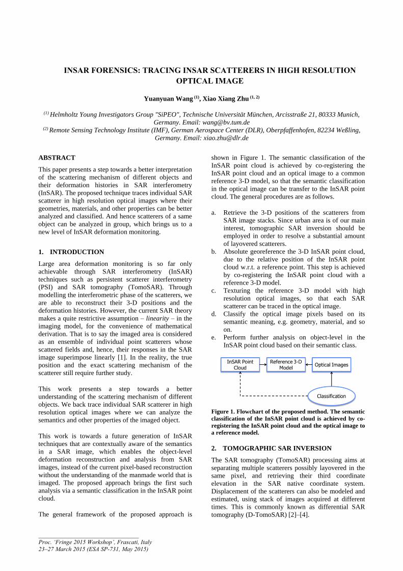
The general framework of the proposed approach is

shown in Figure 1. The semantic classification of the

InSAR point cloud is achieved by co-registering the

InSAR point cloud and an optical image to a common

reference 3-D model, so that the semantic classification

in the optical image can be transfer to the InSAR point

cloud. The general procedures are as follows.

a. Retrieve the 3-D positions of the scatterers from

SAR image stacks. Since urban area is of our main

interest, tomographic SAR inversion should be

employed in order to resolve a substantial amount

of layovered scatterers.

b. Absolute georeference the 3-D InSAR point cloud,

due to the relative position of the InSAR point

cloud w.r.t. a reference point. This step is achieved

by co-registering the InSAR point cloud with a

reference 3-D model.

c. Texturing the reference 3-D model with high

resolution optical images, so that each SAR

scatterer can be traced in the optical image.

d. Classify the optical image pixels based on its

semantic meaning, e.g. geometry, material, and so

on.

e. Perform further analysis on object-level in the

InSAR point cloud based on their semantic class.

Figure 1. Flowchart of the proposed method. The semantic

classification of the InSAR point cloud is achieved by co-

registering the InSAR point cloud and the optical image to

a reference model.

2. TOMOGRAPHIC SAR INVERSION

The SAR tomography (TomoSAR) processing aims at

separating multiple scatterers possibly layovered in the

same pixel, and retrieving their third coordinate

elevation in the SAR native coordinate system.

Displacement of the scatterers can also be modeled and

estimated, using stack of images acquired at different

times. This is commonly known as differential SAR

tomography (D-TomoSAR) [2]–[4].

INSAR FORENSICS: TRACING INSAR SCATTERERS IN HIGH RESOLUTION

OPTICAL IMAGE

_____________________________________ Proc. ‘Fringe 2015 Workshop’, Frascati, Italy 23–27 March 2015 (ESA SP-731, May 2015)

We make use of the D-TomoSAR software Tomo-

GENESIS [5], [6] developed in DLR to process

TerraSAR-X image stacks. For an input data stack,

Tomo-GENESIS retrieves the following information:

the number of scatterers inside each pixel,

the scattering amplitude and phase of each

scatterer,

and their 3D positions and motion parameters, e.g.

linear deformation rate and amplitude of seasonal

motion.

The scatterers’ 3D positions in SAR coordinates can be

converted into a local Cartesian coordinate system, such

as Universal Transverse Mercator (UTM), so that the

results from multiple data stacks with different viewing

angles can be combined. For our test area Berlin, two

image stacks – one ascending orbit, the other

descending orbit – are processed. These two point

clouds are fused to a single one, using a feature-based

matching algorithm which estimates and matches

common building edges in the two point clouds [7]. The

following figure is the fused point cloud which provides

a complete monitoring over the whole city of Berlin.

Figure 2. The fused TomoSAR point cloud of Berlin, which

combines the result from an ascending stack and a

descending stack. The height is color-coded.

3. COREGISTRATION OF TOMOSAR POINT

CLOUDS AND THE REFERENCE MODEL

3.1. CO-REGISTRATION WORKFLOW

Our reference model is a 3D point cloud from an

airborne LiDAR sensor [8], which is represented, same

as the TomoSAR point cloud, in the UTM coordinate

system. And hence, the co-registration problem is the

estimation of translation between two rigid point clouds,

subject to a certain tolerance on rotation and scaling.

However, our LiDAR point cloud is nadir-looking, in

contrast to the side-looking geometry of SAR. In

another word, façade point barely appears in LiDAR

point cloud while it is prominent in TomoSAR point

cloud. This difference is exemplified in Figure 3, where

the left and the right subfigures correspond to the

TomoSAR and LiDAR point clouds of the same area.

These unique modalities have driven our algorithm

developed in the following way:

1 Edge extraction

a. The LiDAR point cloud is rasterized into a 2D

height image.

b. The point density of TomoSAR point cloud is

estimated on the rasterized 2D grid.

c. The edges in the LiDAR height image and the

TomoSAR point density image are detected.

2 Initial alignment

a. Horizontally by cross-correlating the two edge

images.

b. Vertically by cross-correlating the height

histogram of the two point clouds.

3 Refined solution

a. The façade points in both point clouds are

removed.

b. The final solution is obtained using iterative

closest point (ICP) applied on the two reduced

point clouds.

(a)

(b)

Figure 3. (a) TomoSAR point cloud of high-rise buildings,

and (b) the LiDAR point cloud of the same area. Building

façades are almost invisible in the LiDAR point cloud,

while it is prominent in the TomoSAR point cloud.

3.2. 2-D EDGE EXTRACTION

In order to obtain the height image and the point density

image of LiDAR and TomoSAR point clouds

respectively, the two point clouds are tiled according to

a 2D grid. Here we use 2×2 m for our dataset. For the

LiDAR point cloud, the mean height in each grid cell is

computed, while for the TomoSAR point cloud, the

number of points inside the grid cell is counted. The

edges can be extracted from these two images using any

edge detector, such as Sobel filter [9]. The thresholds in

the edge detector are decided adaptively, so that the

Height [m] 122.8

98.7

74.6

numbers of edge pixels in the two edge images are on

the same scale. The following figure is a close up view

of the two edge images near downtown Berlin.

(a)

(b)

Figure 4. (a) A part of the edge image of the reference

LiDAR point cloud in downtown Berlin, and (b) the edge

image of the TomoSAR point cloud roughly at the same

area.

3.3. INITIAL ALIGNMENT

The initial alignment provides an initial solution to the

iterative closest point (ICP) algorithm which is known

to suffer from finding possibly a local minimum. The

initial alignment consists of independently finding the

horizontal and the vertical shifts. The horizontal shift is

found by cross-correlating the edge images of the two

point clouds. In most of the cases, a unique peak can be

found, due to the complex, hence pseudorandom,

structures of a city. Please see Figure 5 for the 2D

correlation of two edge images, where a single

prominent peak is found. The vertical shift is found by

cross-correlating the height histogram of the two point

clouds, which is shown in Figure 6. We also set the bin

spacing of the height histograms to be 2m in our

experiment. The accuracy of the shift estimates are of

course limited by the discretization in the three

directions. However, this is sufficient for the final

estimation.

Figure 5. 2D cross-correlation of the edge images of

TomoSAR and LiDAR point clouds. A single peak is found

at (828, -784) m.

-100 -50 0 50 1000

0.01

0.02

0.03

0.04

Height [m]

De

nsity

TomoSAR Height Histogram

-100 -50 0 50 1000

0.02

0.04

0.06

0.08

0.1

0.12

0.14

Height [m]

De

nsity

LiDAR Height Histogram

-50 0 500

0.1

0.2

0.3

0.4

0.5

0.6

0.7

Shift [m]

Co

rela

tio

n c

oe

ffic

ien

t

Cross-correlation

-100 -50 0 50 1000

0.01

0.02

0.03

0.04

Height [m]

De

nsity

TomoSAR Height Histogram

-100 -50 0 50 1000

0.02

0.04

0.06

0.08

0.1

0.12

0.14

Height [m]

De

nsity

LiDAR Height Histogram

-50 0 500

0.1

0.2

0.3

0.4

0.5

0.6

0.7

Shift [m]

Co

rela

tio

n c

oe

ffic

ien

t

Cross-correlation

(a) (b)

-100 -50 0 50 1000

0.01

0.02

0.03

0.04

Height [m]

De

nsity

TomoSAR Height Histogram

-100 -50 0 50 1000

0.02

0.04

0.06

0.08

0.1

0.12

0.14

Height [m]

De

nsity

LiDAR Height Histogram

-50 0 500

0.1

0.2

0.3

0.4

0.5

0.6

0.7

Shift [m]

Co

rela

tio

n c

oe

ffic

ien

t

Cross-correlation

(c)

Figure 6. (a) The height histogram of TomoSAR point

cloud, (b) the height histogram of LiDAR point cloud, and

(c) the correlation of (a) and (b), where the red cross

marks the peak position which is at -6 m.

3.4. FINAL SOLUTION

The final solution is obtained using a normal ICP

algorithm based on the initial solution calculated from

the previous step. The façade points in the TomoSAR

point clouds are removed to prevent ICP from finding a

wrong solution. The following image demonstrates the

co-registered point cloud. Successful co-registration can

be confirmed by seeing the correct location of the

façade points in Figure 7(b).

(a)

(b)

Figure 7. (a) Close up of the reference LiDAR point cloud

in downtown Berlin, and (b) the co-registered point cloud

combining the TomoSAR and LiDAR point cloud.

4. COREGISTRATION OF OPTICAL

IMAGE AND REFERENCE MODEL

Currently, we rely on the fact that the optical image is

already well co-registered with the reference point

cloud, i.e. the camera extrinsic parameters are well

known in the coordinate system of the reference point

cloud. In our current experiment, the camera position is

known up to an accuracy of 20cm with respect to the

LiDAR point cloud. However, the users are not

restricted to LiDAR point cloud. One can also use a pair

of stereo optical images and the reconstructed 3-D point

cloud.

Figure 8. TomoSAR point cloud textured with the RGB

color from optical image, where the dark background is

the optical image not covered by the point cloud.

Figure 8 is the TomoSAR point cloud textured with

RGB color from the optical image, where the subfigure

(b) is the close up of the area in the dashed red rectangle

in (a). Such textured point cloud enables the analysis of

the SAR point cloud based on the features in optical

image. Currently, we are developing algorithms for co-

registering oblique optical images with 3D model,

which will brings more optical information of façade

points.

5. SEMANTIC CLASSIFICATION IN

OPTICAL IMAGE

The semantic classification is done patch-wised using a

dictionary-based algorithm. The entire optical image is tiled

into small patches, e.g. 50×50 pixels. They are then described

using a dictionary, to be specific, the occurrence of the atoms

in the dictionary. Such model is known as the Bag of Words

(BoW) [10]. The final patch classification is achieved using

support vector machine (SVM). The detailed workflow is as

follows.

5.1. BOW MODEL

BoW originates from text classification, where a text is

modeled as the occurrence of the words in a dictionary,

disregarding the grammar as well as the order. This is also

recently employed in computer vision, especially in image

classification. Analogous to text, the BoW descriptor w of an

image Y is modeled as the occurrence of the “visual” words in

a predefined dictionary D, i.e.:

h D

w Y (1)

where h is the histogram operator, and is the

transformation function from the image space to the feature

space. Hence the visual words refer to the representative

features in the image, whose ensemble constructs the

dictionary.

5.2. FEATURE EXTRACTION

We calculate the dense local features of each patch, i.e.

the feature is computed in a sliding window through the

patch. This is described in Figure 9(a) where the red

window traverses the patch, and computes one local

feature vector at each position. The subfigure (b) is

examples of some other patches extracted from the

image.

Several commonly used features have been tested,

which includes the most popular scale-invariant feature

transform (SIFT) suggested by many literatures.

However, the feature in our experiment is simply the

vectorized the RGB pixel values in a 3×3 sliding

window. Experiment shows its constant robustness and

efficiency for large area processing.

(a) (b)

...

Figure 9. (a) demonstration of dense local feature

computed on an image patch, where the feature is

computed in the red sliding window through the patch,

and (b) some examples of other image patches.

5.3. DICTIONARY LEARNING

Assume the dictionary is defined as N k

D , where N

is the dimension of the word, i.e. feature vector, and k is

the number of feature vectors, also known as atoms. The

k feature vector should include representative features

appear in the whole image, so that each patch can be

well described.

Depending on the patch size, certain number of feature

vectors is obtained from each patch. Collecting all of

them for all the patches should already give a

preliminary dictionary. However, the size of such

dictionary is tremendous, knowing that an aerial optical

image can be tiled into millions of patches, and each

patch can give tens to hundreds of feature vectors. This

renders k in the order of hundreds of million.

Therefore, the dimension of the preliminary dictionary

should be reduced. We perform an unsupervised

clustering, e.g. k-means, on the preliminary dictionary

in order to quantize the feature space. The cluster center

is extracted as the final dictionary. Figure 10 exemplify

the quantization in a 2-D feature space. The colored

crosses are the features extracted from the whole image.

5.4. PATCH DESCRIPTOR

The patches are described following Equation (1).

Implementation-wise, this is achieved by assigning the

features of a patch to their nearest neighbours in the

dictionary. To this end, the patch descriptor is a vector k

v .

Figure 10. Demonstration of dictionary learning in two

dimensional feature space. The colored crosses are the

features collected from all the patches in the image. A k-

means clustering is performed to get k cluster centers, i.e.

the dictionary atoms. Image modified from [11].

5.5. CLASSIFICATION

The classification is done using a linear SVM [12]

implemented in an open source library VLFeat [13].

The SVM classifier finds a hyperplane which separates

two classes of training samples with maximal margin.

Giving the patch descriptor v, its SVM classification is:

Tf sign b v w v (2)

where kw and b are the parameters of the

hyperplane, and sign is the sign operator which

outputs ±1.

For an m-class (m>2) problem, difference SVM should

be trained for each class against the rest. The final

classification of a patch v is assigned to the one with the

largest SVM score, i.e.:

maxT

f v W v b (3)

where k mW and m

b are the concatenated

parameters of m hyperplanes.

Our test image (5000×5000) is tiled into patches of

50×50 pixel, with 46 pixel overlap. That is to say, the

classification of each patch is only assigned to the 4×4

pixel in the center. Among all the patches, 570 are

manually selected as training samples. Four classes are

preliminarily defined: building, roads/rail, river, and

vegetation. Each of them has 240, 159, 39, and 132

training patches, respectively. The feature in our

experiment is simply the vectorized RGB pixel values in

a 3×3 sliding window, which results in a feature space

of 27 dimension. Figure 11 shows the classification

result of a region in the entire image, where the left

image is the optical image, and in the right image,

classified building, road, river, and vegetation are

marked as red, blue, green, and blank. Despite the

extremely simple feature we used, the four classes are

very well distinguished.

(a) (b)

Figure 11. (a) the test optical image, and (b) the

classification of building, road, river, and vegetation,

where they are colored in red, blue, green, and blank.

Since we are particularly interested in building, its

classification performance is evaluated by classifying

half of training samples using the SVM trained with the

other half of the samples. The average precision of the

current algorithm is 98%. The full precision and recall

curve is plotted in Figure 12(a). The equivalent receiver

operating characteristic curve is also shown in Figure

12(b), for the readers who are more familiar with it. The

red cross marks our decision threshold which gives a

detection rate of 90%, and false alarm rate of 3%.

0 0.2 0.4 0.6 0.8 10

0.1

0.2

0.3

0.4

0.5

0.6

0.7

0.8

0.9

1

Recall

Pre

cis

ion

PR curve

0 0.2 0.4 0.6 0.8 10

0.1

0.2

0.3

0.4

0.5

0.6

0.7

0.8

0.9

1ROC curve

False alarm rateD

ete

ction r

ate

0 0.2 0.4 0.6 0.8 1

0

0.1

0.2

0.3

0.4

0.5

0.6

0.7

0.8

0.9

1

Recall

Pre

cis

ion

PR curve

0 0.2 0.4 0.6 0.8 10

0.1

0.2

0.3

0.4

0.5

0.6

0.7

0.8

0.9

1ROC curve

False alarm rate

Dete

ction r

ate

(a) (b)

Figure 12. (a) precision and recall curve of the building

classification with an average precision is 98%, and (b) the

ROC curve of the classification. The red cross marks our

decision point which gives a detection rate of 90%, and

false alarm rate of 3%.

6. OBJECT-LEVEL ANALYSIS

Based on the semantic classification, we can extend the

current pixel-based monitoring and manual selection of

region of interest to a systematic monitoring on an

object-level. In the following, examples on bridge and

railway monitoring are exemplified.

6.1. AUTOMATIC RAILWAY MONITORING

We applied the semantic classification scheme on an

orthorectified optical image centered at the Berlin

central station. We particularly classified the railway

and river class for the following analysis. Figure 13

shows the classification map where the railway class

and river class are labelled in green and red,

respectively. The classification performance is

consistent with the evaluation shown in Figure 12.

Some false alarm appeared as small clusters, but they

can be removed by post-processing.

Figure 13. River (red) and railway (green) classified using

the BoW method. The classification performance is

consistent as the evaluation in Figure 12 shows. Some false

alarm appeared as small clusters. They can be filtered out

in post-processing.

Based on the classification, the corresponding points in

the TomoSAR point cloud can be extracted. Assuming

the railway is smooth and continuous, a smooth spline

function was fitted to the x and y (east and north)

coordinates of the railway points to connect separated

segments, i.e.:

2 2

2 2ˆ arg min 1

ss y s s (4)

where y is the y coordinates of the railway points, s is

the spline function (quadratic or cubic) w.r.t. the x

coordinates of the railway points, and 0,1 is the

smoothing parameter. The smooth spline is centered in

the railway, and the width of the railway is adaptively

estimated at each position. Therefore, we are able to

interpolate the discontinuity of the railway due to the

presence of the Berlin central station. Figure 14(a) shows

the connected railway points overlaid on a calibrated

aerial image of 20cm ground resolution. The color

shows the amplitude of seasonal motion due to the

thermal expansion of the steel. The motion parameters

have been filtered by minimizing the total variation.

The seasonal motion shows a regular pattern along the

railway, which is because of the expansion and

contraction of individual railway section. By detecting

the peaks in the derivative, the joints of railways can be

detected, which are shown as the green dots in Figure

14(b). In subfigure (c), we provide the close up view of

the two joints in the optical image where the railway

joint shown up as dark lines are both visible.

6.2. AUTOMATIC BRIDGE MONITORING

By analysing the discontinuity of the river segmentation

and assuming the discontinuities are caused by bridges,

the bridges’ positions can be detected automatically.

The corresponding bridge points are extracted from the

TomoSAR point cloud, and projected to the optical

image.

The projected bridge points are shown in Figure 15

where the color also represents the amplitude of

seasonal deformation. The upper most bridge belongs to

a segment of the railway which is known to have

thermal expansion. The middle bridge undergoes a 5mm

seasonal motion at its west end and 2mm at the east end.

This suggests a more rigid connection of the bridge with

the foundation at its east end. The two lower bridges are

stable according to the motion estimates.

-5 0 5 [mm]

(a)

(b)

(c)

Figure 14. (a) Connected railway points extracted from the

TomoSAR point cloud. The color shows the amplitude of

seasonal motion due to the thermal expansion of the steel,

(b) the amplitude of seasonal motion filtered by

minimizing the total variation, (c) the detected railway

joints marked in green, and (d)

-5 0 5 [mm]

Figure 15. Overlay of the amplitude of seasonal motion of

brides extracted from the TomoSAR point cloud on the

optical image. The bridges are automatically detected from

the classification map shown in Figure 13 using

discontinuity analysis.

7. CONCLUSION

This paper is the first semantic analysis of high

resolution InSAR point cloud in urban area. Through

co-registering optical image and InSAR point cloud to a

common reference 3-D model, we are able to relate the

semantic meaning extracted from the optical image to

the InSAR point cloud. The complementary information

provided by the two data types enables an object-level

InSAR deformation and 3-D analysis.

In the future, we aim at a more intelligent system by

including more semantic classes, such as high-rise

buildings, residential area, or even specific landmarks,

and so on. To reduce the human interaction, we are also

aiming at a completely unsupervised semantic

classification.

8. ACKNOWLEDGEMENT

This work was supported by the Helmholtz Association

under the framework of the Young Investigators Group

“SiPEO” (VH-NG-1018, www.sipeo.bgu.tum.de),

International Graduate School of Science and

Engineering, Technische Universität München (Project

6.08: “4D City”), and the German Research Foundation

(DFG, Förderkennzeichen BA2033/3-1).

9. REFERENCES

[1] R. Bamler and P. Hartl, “Synthetic aperture radar

interferometry,” Inverse Probl., vol. 14, no. 4, p.

R1, 1998.

[2] F. Lombardini, “Differential tomography: a new

framework for SAR interferometry,” IEEE Trans.

Geosci. Remote Sens., vol. 43, no. 1, pp. 37–44,

Jan. 2005.

[3] G. Fornaro, et al., “Four-Dimensional SAR

Imaging for Height Estimation and Monitoring of

Single and Double Scatterers,” IEEE Trans.

Geosci. Remote Sens., vol. 47, no. 1, pp. 224–237,

Jan. 2009.

[4] X. X. Zhu and R. Bamler, “Very High Resolution

Spaceborne SAR Tomography in Urban

Environment,” IEEE Trans. Geosci. Remote

Sens., vol. 48, no. 12, pp. 4296–4308, 2010.

[5] X. Zhu, Very High Resolution Tomographic SAR

Inversion for Urban Infrastructure Monitoring: A

Sparse and Nonlinear Tour, vol. 666. Deutsche

Geodätische Kommission, 2011.

[6] X. Zhu, et al., “Tomo-GENESIS: DLR’s

Tomographic SAR Processing System,” in Urban

Remote Sensing Event (JURSE), 2013 Joint,

2013, pp. 159–162.

[7] Y. Wang and X. X. Zhu, “Automatic Feature-

based Geometric Fusion of Multi-view TomoSAR

Point Clouds in Urban Area,” IEEE J. Sel. Top.

Appl. Earth Obs. Remote Sens., vol. PP, no. 99,

2014.

[8] “Data provided by ‘Land Berlin’ and ‘Business

Location Service’, supported by ‘Europäischer

Fonds für Regionale Entwicklung’.” .

[9] I. Sobel, “An Isotropic 3x3 Image Gradient

Operator,” Present. Stanf. AI Proj. 1968, 2014.

[10] G. Csurka, et al., “Visual categorization with bags

of keypoints,” in Workshop on statistical learning

in computer vision, ECCV, 2004, vol. 1, pp. 1–2.

[11] S. Cui, “Spatial and temporal SAR image

information mining,” Universität Siegen, Siegen,

Germany, 2014.

[12] C. Cortes and V. Vapnik, “Support-vector

networks,” Mach. Learn., vol. 20, no. 3, pp. 273–

297, Sep. 1995.

[13] B. F. Andrea Vedaldi, “VLFeat: an open and

portable library of computer vision algorithms.,”

in Proceedings of the 18th International

Conference on Multimedea 2010, Firenze, Italy,

2010, pp. 1469–1472.