Insights in uncertainty

of source parameters :

combining historical

eyewitness accounts on

tsunami-induced wave

heights and numerical

simulation

J. Rohmer, M. Rousseau, A. Lemoine, J. Lambert, R.

Pedreros, B. Aalae

> 1

Contexte

> 2

> 3

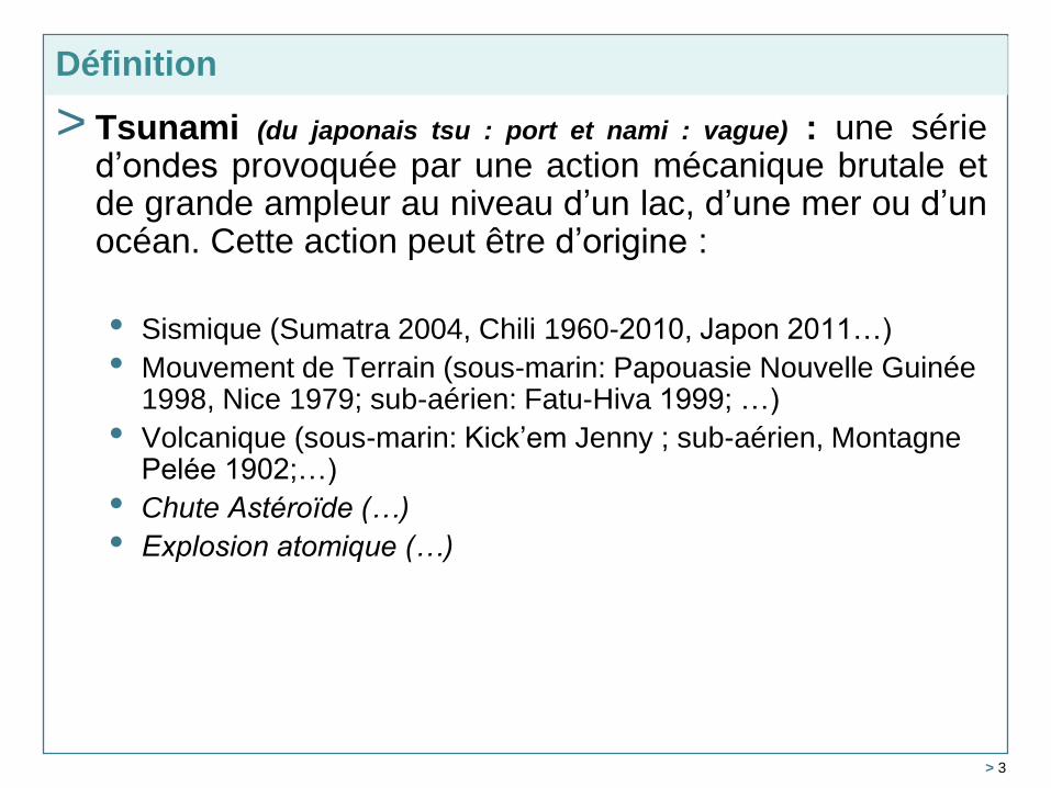
> Tsunami (du japonais tsu : port et nami : vague) : une série d’ondes provoquée par une action mécanique brutale et de grande ampleur au niveau d’un lac, d’une mer ou d’un océan. Cette action peut être d’origine :

• Sismique (Sumatra 2004, Chili 1960-2010, Japon 2011…)

• Mouvement de Terrain (sous-marin: Papouasie Nouvelle Guinée 1998, Nice 1979; sub-aérien: Fatu-Hiva 1999; …)

• Volcanique (sous-marin: Kick’em Jenny ; sub-aérien, Montagne Pelée 1902;…)

• Chute Astéroïde (…)

• Explosion atomique (…)

Définition

Origine sismique

> 4

Génération Propagation Inondation

Trois phases

> 5

Schéma de propagation d’un tsunami depuis le milieu profond vers la côte

Source : http://www.prh.noaa.gov/itic/fr/library/pubs/great_waves/tsunami_great_waves.html

- Longueur d’onde : km – centaines de km

- Période : quelques minutes – une heure

De la génération à l’inondation

> 6

élévation de la surface d’eau Grille mère (9km)

Grille fille (2km)

Generation (Okada 1985) and propagation (Funwave-TVD) up to French

Polynesia

> 7

Simulation of the tsunami generated in Chili in 1960

Recent observations due to tsunamis in France

> 8

In tsunami hazard assessment,

• Major source of uncertainty = earthquake source

parameters

• Those parameters strongly influence the tsunami-induced

sea surface elevation SSE

Combining simulations with observations can

improve knowledge and constrain those uncertainties

Challenges:

1. Observations on past events scarce and imprecise

2. CPU time cost of one simulation several hours

Context and problem definition

> 9

Tsunami Ligure 1887

> 10

earthquake

The 1887 Ligurian event Damaging historical earthquake occuring at the junction

between the southern French-Italian Alps and Ligurian basin

induced tsunami

Motivating case study

La

rro

qu

e e

t a

l. 2

01

2

Mw = 6.7- 6.9 (current estimation)

> 11

Lon

(°)

Lat

(°)

Depth Z

(m)

Azim (°)

2 scenarios

North (South) dipping

DIP

(°)

Rake

(°)

Average

displacement

D (m)

Length

(m)

Width

(km)

7.78 43.45 5 220 (40) 10 70 0,3 20 10

8.15 43.92 20 260 (80) 70 110 2 57 22

Uncertainty characterisation

Based on Larroque et al. (2012) and Ioualalen et al. (2014)

> 12

Location orientation geometry

Some illustrative results

MAX sea surface elevation SSE

Averaged over 300 simuls

MODEL CHARACTERISTICS

2,650,000 mesh cells

CPU time of a single simulation 30 min with 4*24 cores

Funwave_TVD Boussinesq ocean surface wave propagation + Okada for initial

deformation

> 13

300 configurations were randomly generated (latin hypercube sampling and uniform

distribution).

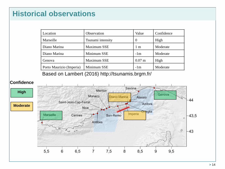
Location Observation Value Confidence

Marseille Tsunami intensity 0 High

Diano Marina Maximum SSE 1 m Moderate

Diano Marina Minimum SSE -1m Moderate

Genova Maximum SSE 0.07 m High

Porto Maurizio (Imperia) Minimum SSE -1m Moderate

Historical observations

Based on Lambert (2016) http://tsunamis.brgm.fr/

High

Moderate

Confidence

> 14

Simulation results (a priori)

Observation

Assumed range of uncertainty

> 15

Over

Over Under

Under

Metamodelling principles

> 16

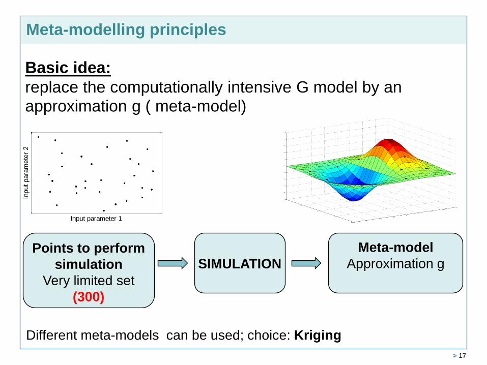
Basic idea:

replace the computationally intensive G model by an approximation g ( meta-model)

Points to perform

simulation

Very limited set

(300)

Meta-model

Approximation g

Input parameter 1

Input

para

mete

r 2

SIMULATION

Different meta-models can be used; choice: Kriging

Meta-modelling principles

> 17

Kriging-based meta-modelling

> Consider f the unknown function Hs=f(x) with Hs the

response, x the uncertain cyclone characteristic;

> 18

> Without any knowledge (no simulation), assume:

with m the mean; Z(.) is a centered stationary gaussian

process GP with C the covariance function:

with ² the process total variance and R the correlation function

e.g., [Forrester et al. 2008]

Kriging-based meta-modelling

)()( xx ZmHS

)R();C( )2()1(2)2()1(xxxx

> 19

> Without any knowledge (no simulation), assume:

with m the mean; Z(.) is a centered stationary gaussian

process GP with C the covariance function:

with ² the process total variance and R the correlation function

²=1; lengthscale =1 e.g., [Forrester et al. 2008]

Kriging-based meta-modelling

Covariance function Example of 1 random sample

)()( xx ZmHS

)R();C( )2()1(2)2()1(xxxx

> 20

> A priori knowledge, 50 random samples

Large

dispersion

Kriging-based meta-modelling

> 21

> Let us run 6 simulation scenarios X;

> HD =set of model results (= knowledge on the unknown simulator).

At the cost of CPU

time!

Kriging-based meta-modelling

> 22

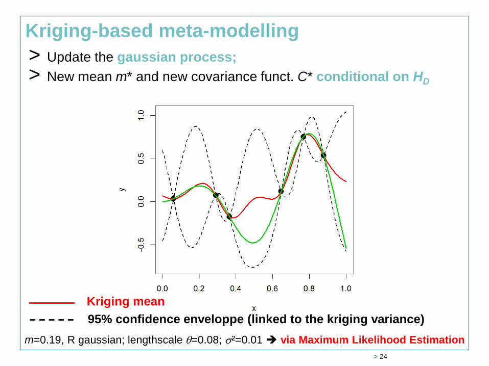
> Update the gaussian process;

> New mean m* and new covariance funct. C* conditional on HD.

m=0.19, R gaussian; lengthscale =0.08; ²=0.01 via Maximum Likelihood Estimation

Kriging-based meta-modelling

> 23

Kriging mean

95% confidence enveloppe (linked to the kriging variance)

> Update the gaussian process;

> New mean m* and new covariance funct. C* conditional on HD

m=0.19, R gaussian; lengthscale =0.08; ²=0.01 via Maximum Likelihood Estimation

Kriging-based meta-modelling

> 24

Strategy

> 25

> Simulate tsunami-induced sea surface elevation H ( max

/ min) using 300 different configurations of earthquake

source via Latin Hypercube Sampling

• Use of Promethee environment (IRSN, Y. Richet)

• lhs R package

Proposed Strategy

> 26

> Simulate tsunami-induced wave height H ( max / min)

using 300 different configurations of earthquake source

via Latin Hypercube Sampling

> Build a 9-dimensional kriging meta-model

• DiceKriging R package (Roustant et al., 2012)

• Matern covariance, linear trend, no nugget, MLE estimation

Proposed Strategy

> 27

> Simulate tsunami-induced wave height H ( max / min)

using 300 different configurations of earthquake source

via Latin Hypercube Sampling

> Build a 9-dimensional kriging meta-model

> Validate via LOOCV (Leave-One-Out-Cross-Validation,

compute R²)

Proposed Strategy

> 28

Validation of kriging metamodel – N. dipping model

R²=89% R²=88% R²=89%

R²=91% R²=84% R²=92.5%

Satisfactory approximation quality (typical threshold at 80%, see e.g., Marrel et al.,

(2009); Storlie et al. (2009)

> 29

> Simulate tsunami-induced sea surface elevation H ( max

/ min) using 300 different configurations of earthquake

source via Latin Hypercube Sampling

> Build a 9-dimensional kriging meta-model

> Validate via LOOCV (Leave-One-Out-Cross-Validation,

compute R²)

> Perform Bayesian Inference using ABC methods (e.g.

Marin et al., 2012) • 1 million of simulations using Sobol’ sequence (randtoolbox R package)

• Abc & abctools R package

Proposed Strategy

biasSourcebiassimulatedobserved HHH )(ˆ

> 30

Bayesian inference

> 31

Bayesian inference - principles

)()()( obsobs HppHp

Prior

knowledge

Update of

probability

information

on after

observing H

Likelihood =

probability of

observing H

given

Likelihood function usually hard to compute

> 32

Approximate Bayesian Computation ABC

Wilkinson (2015) > 33

Approximate Bayesian Computation ABC

Wilkinson (2015) > 34

Approximate Bayesian Computation ABC

=5

Wilkinson (2015) > 35

Approximate Bayesian Computation ABC

=2.5

Wilkinson (2015) > 36

Approximate Bayesian Computation ABC

=1

Wilkinson (2015) > 37

Diagnostic of ABC - example

Prangle et al. (2014)

Distribution should be uniform

Choosing the proportion of accepted samples

Initial number of random samples = 1 million

Verifying the coverage property (Prangle et al. 2014)

> 39

A Posteriori distributions

1,000 accepted random samples

> 40

Inference of source parameters

> 41

Influence of ABC tuning

> 42

Inference of magnitude - North Dipping model

In agreement with past studies: 6.7-6.9 (Ioualalen et al. (2014)

> 43

Inference of bias parameters

biasSourcebiassimulatedobserved HHH )(ˆ

> 44

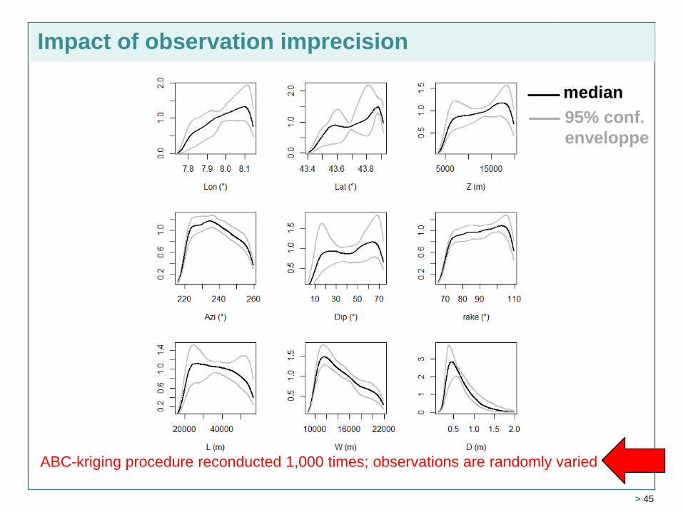
ABC-kriging procedure reconducted 1,000 times; observations are randomly varied

Impact of observation imprecision

median

95% conf.

enveloppe

> 45

> Methodology for combining imprecise

observations and numerical simulations

> Emulation of the long running numerical

simulator (meta-model)

> Further work • Inferring assumption scenarios i.e. complex fault geometry

• Impact of metamodel error

Summary

> 46

Ioualalen et al. (2014

THANK YOU

> 47

Influence of meta-model error

> 48