Lab test report and recommendations Deliverable report D5.2
Deliverable Report: Final version, issue date November 30th, 2016
INSITER - Intuitive Self-Inspection Techniques using Augmented Reality for construction, refurbishment and maintenance of energy-efficient buildings made of
prefabricated components.
This research project has received funding from the European Union’s H2020 Framework Programme for research and innovation under Grant Agreement no 636063.
INSITER - D5.2- Lab test report and recommendations– November 2016
page 2
Issue Date November 2016 Produced by UNIVPM (P9) Main authors Gian Marco Revel, Milena Martarelli, (UNIVPM)
Giuseppe Pandarese, Antonio D’Antuono Co-authors Jacques Cuenca (SWS)
Pedro Lerones (CARTIF) Jan-Derrick Braun (HVC)
Version: Final Reviewed by Klaus Luig (3L)
Benedetta Marradi (AICE) Approved by Rizal Sebastian (DMO, Technical Coordinator)
Ton Damen (DMO, Project Coordinator) Dissemination Public
Colophon Copyright © 2016 by INSITER consortium
Use of any knowledge, information or data contained in this document shall be at the user's sole risk. Neither the INSITER Consortium nor any of its members, their officers, employees or agents accept shall be liable or responsible, in negligence or otherwise, for any loss, damage or expense whatever sustained by any person as a result of the use, in any manner or form, of any knowledge, information or data contained in this document, or due to any inaccuracy, omission or error therein contained. If you notice information in this publication that you believe should be corrected or updated, please contact us. We shall try to remedy the problem.
The authors intended not to use any copyrighted material for the publication or, if not possible, to indicate the copyright of the respective object. The copyright for any material created by the authors is reserved. Any duplication or use of objects such as diagrams, sounds or texts in other electronic or printed publications is not permitted without the author's agreement.
This research project has received funding from the European Union’s H2020 Framework Programme for research and innovation under Grant agreement no 636063.
Lab test report and recommendations Deliverable report D5.2
INSITER - D5.2- Lab test report and recommendations– November 2016
page 3
Publishable executive summary
The main goal of INSITER research on the measurement devices is: to optimise the measurement procedures to suit the
use for on-site self-inspection. The current procedures are either too complex or take too much time to be applied during
on-site construction process. The Lab Testing shows that the INSITER’s innovation, which comprises optimised
measurement procedure, is adequate for on-site self-inspection. After successful Lab Testing, these procedures will be
tested, validated and demonstrated in factory and field situation respectively.
The main scope of D5.2 is to report the lab tests performed to validate the selected protocols described in D5.1 and the
recommendation arisen in view of the application to the real test cases. The lab tests had the aim to implement in a
controlled environment the protocols and methodologies related to the INSITER self-inspection system and to identify
eventual problems that can be encountered in construction sites.
Within the INSITER project, 7 test cases have been defined, namely: Test case 1 – Thermal test case; Test case 2 –
Acoustic test case; Test case 3 – Air tightness test case; Test case 4 – Humidity test case; Test case 5 – Geometry test
case; Test case 6 – BIM test case; and Test case 7 – Augmented Reality test case. The test cases 4, 5, 7 have been
described in the previously submitted deliverable D5.1 (approved by European Commission). This deliverable is focused
on the remaining test cases and on test for MEP/HVAC components, based on humidity and geometrical aspects.
Therefore, the main topics tackled are:
- Description of the test cases developed at laboratory level for the validation of the procedures for thermal,
acoustic and air leakage assessment (Test case 1, 2 and 3). Those tests have been performed in the cooling
room at the UNIVPM laboratory.
- Reporting of the use of the 3D laser scanner for the inspection of MEP/HVAC in terms of installation and humidity
performances. Those tests have been carried out by CARTIF in its CARTIF-3 Building.
- Connection between experimental data and BIM which has been developed by HOCHTIEF.
- Evidencing the main recommendations for the use of the INSITER protocols in the factory.
The main achievement of the deliverable is the applicability of the INSITER diagnostic tools for different measurement
aspects assessment and the main advantages/disadvantages of those techniques with respect to the currently available
in terms of the measurement aspects addressed.
Concerning the thermal transmittance the IR camera based soft sensing procedure allows to reducing the testing time by
keeping the same level of accuracy. The current standard for in-situ thermal transmittance measurement by means of
heat flow meter (ISO 9869) states that the U-value can be evaluated with an accuracy of about 8%, depending on the
environmental conditions. The inspection time is a function of the building element thermal phase (or time shift related to
its thermal inertia) and is influenced by the stability of the natural day cycle. The standard, in fact, is based on natural
day cycles for the generation of a gradient between the internal and external surface of the building element. The
minimal inspection time declared is of 72 h but the test can be stopped only if the U-value do not change more than 5%
for three consecutive nights. Standard testing time is between 7 and 15 days. The IR camera soft-sensing method
proposed as INSITER thermal transmittance measurement system is based on forced thermal cycles and an
accompanying model which allows to decrease the testing time up to some cycles (between 20 and 60 hours) depending
INSITER - D5.2- Lab test report and recommendations– November 2016
page 4
on the thermal phase of the building element (4 h for a concrete wall or 10 h for an high insulation wall, respectively).
The cost of the equipment used in the current standard (ISO 9869) is of about 3000€ (cost of the heat flow meter) even
though is strongly suggested to use an IR thermal camera to accurately position the heat flow meter on an region free of
thermal bridges. The cost of the thermal transmittance tools proposed by INSITER is of about 5000€ (cost of the thermal
camera). The same tool proposed by INSITER for the thermal transmittance evaluation (IR camera) is used for thermal
bridge estimation and quantitative effect estimation on the global transmittance. The current standard ISO 14683 allow
estimating the linear thermal transmittance of thermal bridges in building construction by numerical calculation. The
INSITER procedure is based instead on real measurements.
Concerning the acoustic aspect the tools proposed by INSITER are the SoundBrush and the acoustic beamforming for
acoustic leakages identification. The first has the main advantage of having installed a tracking device able to localize
the measurement position in relation to the testing element. The positioning system has been interfaced with the BIM in
order to easily superimpose the measurement data to the 3D model. Beamforming also called acoustic camera is
powerful tool since, as the name states, allows visualising acoustic fields and therefore localising sound insulation losses
or acoustic leaks, superimposing them onto the visual image of the building component.
Finally, the method proposed as INSITER tool for air leakages localisation is an improvement of the current standard
based on blower door test (EN ISO 9972) which allows only to assess if air leakages are present but not to identify their
spatial position. INSITER proposes to use ultrasound probes to localise in spade air leakages of approximately 3-20 mm
width. Only with sensors working in the ultrasonic frequency range (20-100 kHz), it is possible to identify such tiny cracks
thanks to the small wavelength of the ultrasonic waves. For bigger cracks or gaps between building elements the tools
proposed by INISTER for acoustic aspects assessment can be applied indifferently. Since they are working on a
frequency range up to 10 kHz they are suitable for the detection of gaps larger than about 30 mm.
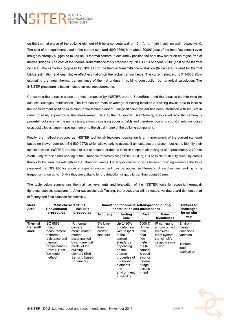
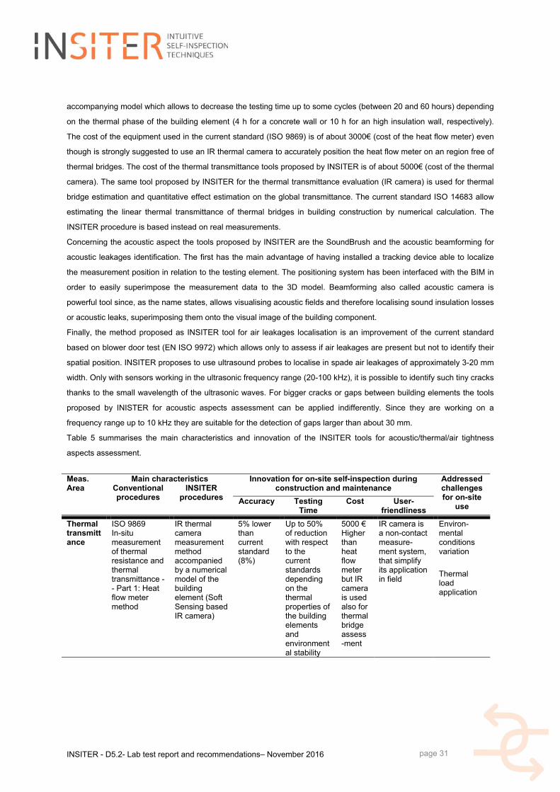
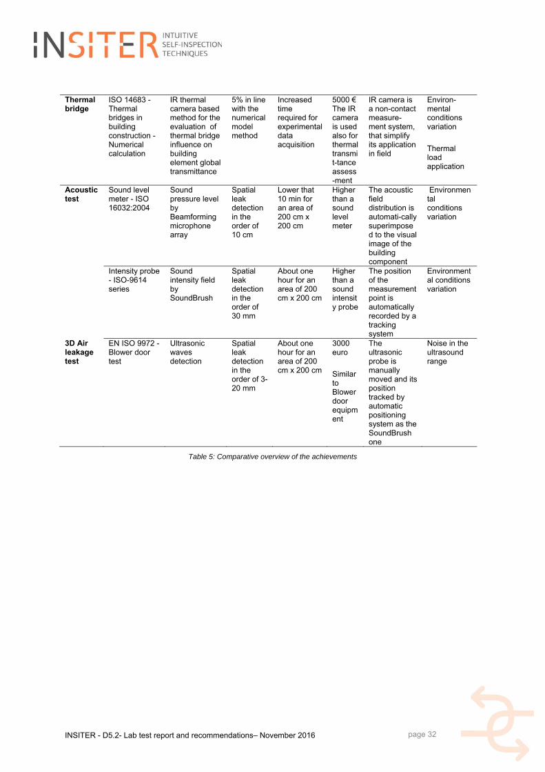
The table below summarises the main achievements and innovation of the INSITER tools for acoustic/thermal/air
tightness aspects assessment. After successful Lab Testing, the procedures will be tested, validated and demonstrated
in factory and field situation respectively.
Meas. Area
Main characteristics Innovation for on-site self-inspection during construction and maintenance
Addressedchallenges for on-site
use
Conventional procedures
INSITER procedures Accuracy Testing
Time Cost User-
friendliness
Thermal transmittance
ISO 9869 In-situ measurement of thermal resistance and thermal transmittance -- Part 1: Heat flow meter method
IR thermal camera measurement method accompanied by a numerical model of the building element (Soft Sensing based IR camera)
5% lower than current standard
Up to 50% of reduction with respect to the current standards depending on the thermal properties of the building elements and environmental stability
5000 € Higher than heat flow meter but IR camera is used also for thermal bridge assess-ment
IR camera is a non-contact measure-ment system, that simplify its application in field
Environ-mental conditions variation
Thermal load application
INSITER - D5.2- Lab test report and recommendations– November 2016
page 5
Thermal bridge
ISO 14683 - Thermal bridges in building construction -Numerical calculation
IR thermal camera based method for the evaluation of thermal bridge influence on building element global transmittance
5% in line with the numerical model method
Increased time required for experimental data acquisition
5000 € The IR camera is used also for thermal transmit-tance assess-ment
IR camera is a non-contact measure-ment system, that simplify its application in field
Environ-mental conditions variation
Thermal load application
Acoustic test
Sound level meter - ISO 16032:2004
Sound pressure level by Beamforming microphone array
Spatial leak detection in the order of 10 cm
Lower that 10 min for an area of 200 cm x 200 cm
Higher than a sound level meter
The acoustic field distribution is automati-cally superimposed to the visual image of the building component
Environ-mental conditions variation
Intensity probe - ISO-9614 series
Sound intensity field by SoundBrush
Spatial leak detection in the order of 30 mm
About one hour for an area of 200 cm x 200 cm
Higher than a sound intensity probe
The position of the measurement point is automatically recorded by a tracking system
Environ-mental conditions variation
3D Air leakage test
EN ISO 9972 -Blower door test
Ultrasonic waves detection
Spatial leak detection in the order of 3-20 mm
About one hour for an area of 200 cm x 200 cm
3000 euro
Similar to Blower door equipment
The ultrasonic probe is manually moved and its position tracked by automatic positioning system as the SoundBrush one
Noise in the ultrasound range
INSITER - D5.2- Lab test report and recommendations– November 2016
page 6
List of acronyms and abbreviations
Abbreviation /
acronym
Description
2D Two-Dimensional
3D Three-Dimensional
4D Four-Dimensional
AR Augmented Reality
BIM Building Information Modelling
CAD Computer Aided Design
CF Solar Correction Factor
ETTV Envelope Thermal Transfer Value
FOV Field of View
IFOW Instantaneous Field of View
GPS Geographic Positioning System
GRC Glass Reinforced Concrete
HDCAM High Definition Camera
HVAC Heating, Ventilation, Air Conditioning
IR Infrared
JSCAD 3D model format for the software OpenJSCAD
L Index of reflectivity
MEMS Micro Electro-Mechanical Systems
MEP Mechanical, Electrical, Plumbing
QR Quick Response
RMS Root Mean Square
RTK Real Time Kinematic
SC Solar Coefficient
SNR Signal to Noise Ratio
STL STereo Lithography interface format
X3D File format
INSITER - D5.2- Lab test report and recommendations– November 2016
page 7
Table of Contents
1. INTRODUCTION 9
1.1 Objectives and structure of this deliverable 9
1.2 R&D methodology employed to achieve results presented in this deliverable 9
1.3 Main achievements and limitations 10
2. LAB TEST 11
2.1 3D thermal test 11
2.1.1 3D thermal maps 13
2.1.2 Image processing for SNR improvement 17
2.2 3D Acoustic test 18
2.2.1 Experimental setup- sound intensity measurement – SoundBrush 18
2.2.2 Exporting SoundBrush data as a 3D model 20
2.2.3 Sound source localisation – acoustic array 22
2.2.4 Sound source localisation results - leakage at the top of the panel side 23
2.2.5 Observation of leakage across the entire panel-room junction 25
2.2.6 Sound intensity results - leakage from the panel-mock-up junction 26
2.2.7 Determination of the sound transmission loss 27
2.3 3D air leakage test 28
2.4 Comparative overview of the achievements 30
3. INSPECTION & INSTRUCTION INFORMATION FOR MEP/HVAC INSTALLATIONS 33
3.1 Use of 3D reflectivity information for MEP/HVAC inspection and instruction 33
3.2 Use of 3D geometric information for MEP/HVAC inspection and instruction 36
4. VIRTUAL/REAL TESTING OF QUALITY AND PERFORMANCE LEVELS BASED ON BIM 43
4.1 Prove models to guarantee smooth BIM processes 43
4.1.1 Model checks -> processes (naming conventions, data availability, attributes) 43
4.1.2 Deviation analysis -> Augmented Reality (geometrical exactness) 43
4.1.3 4D checks -> sequences (logical correctness of time schedules) 43
4.2 Validate the representation of results created by the other test cases 43
4.2.1 Provide data via BIM (additional documents, attribute values, links) 43
4.2.2 Provide model check results (Feedback on model analysis) 44
4.2.3 Results of a deviation analysis(Feedback on geometrical exactness) 44
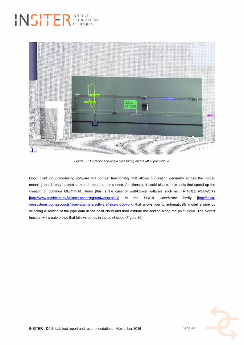
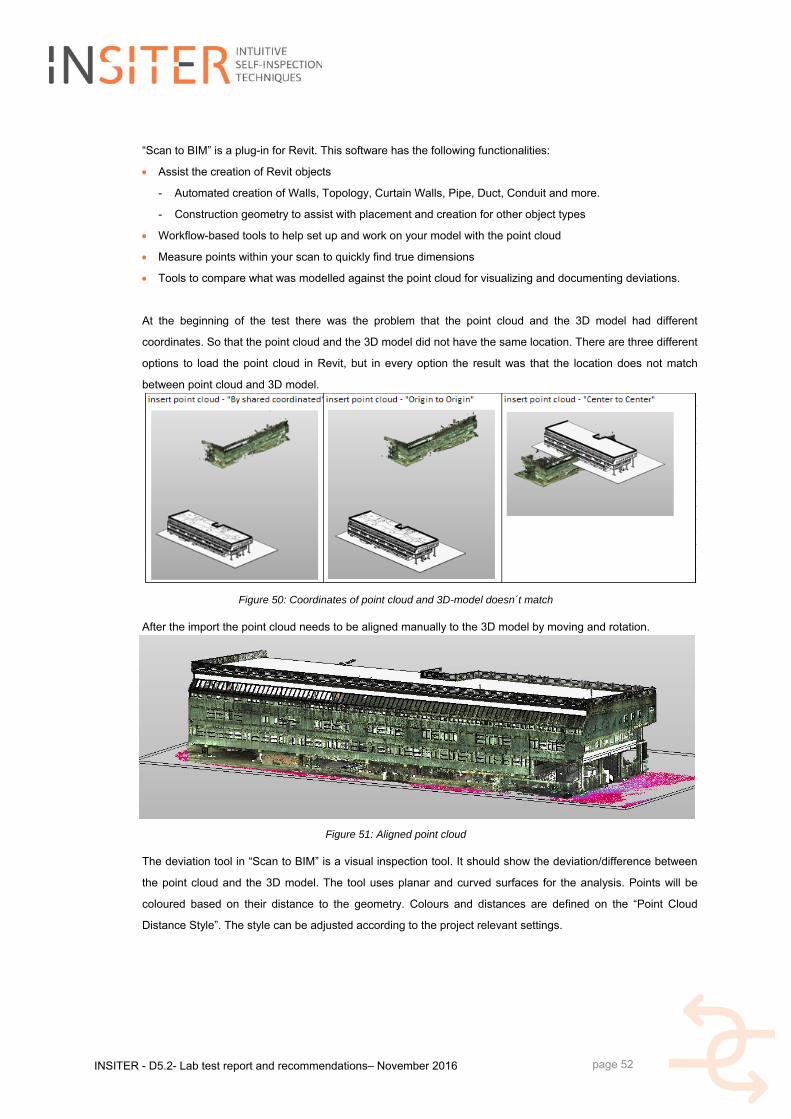
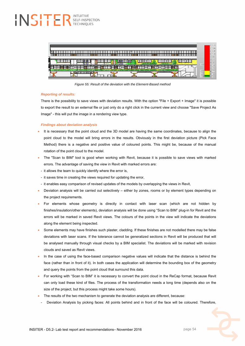
4.3 Use Case Scenario Examples 44
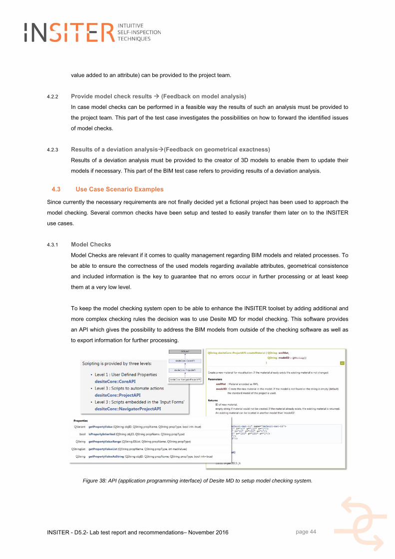
4.3.1 Model Checks 44
4.3.2 Deviation analysis 51
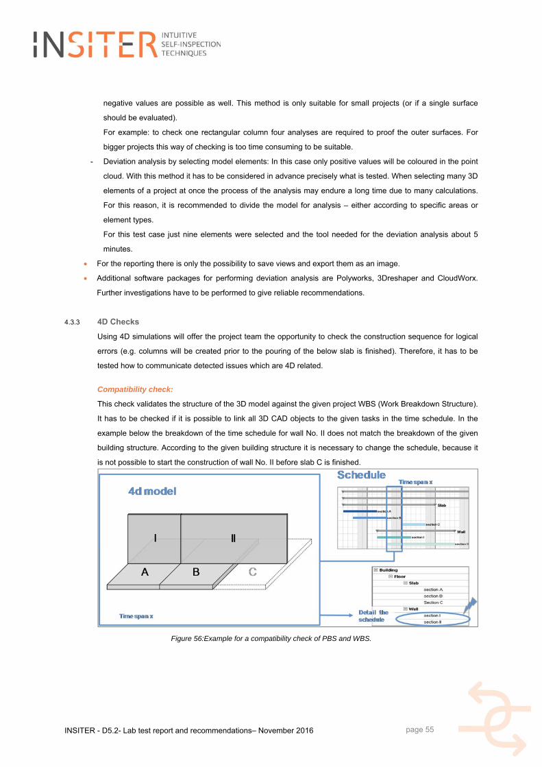
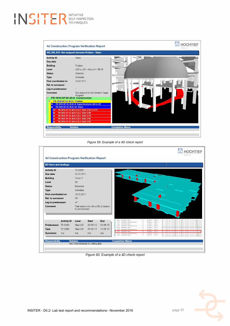
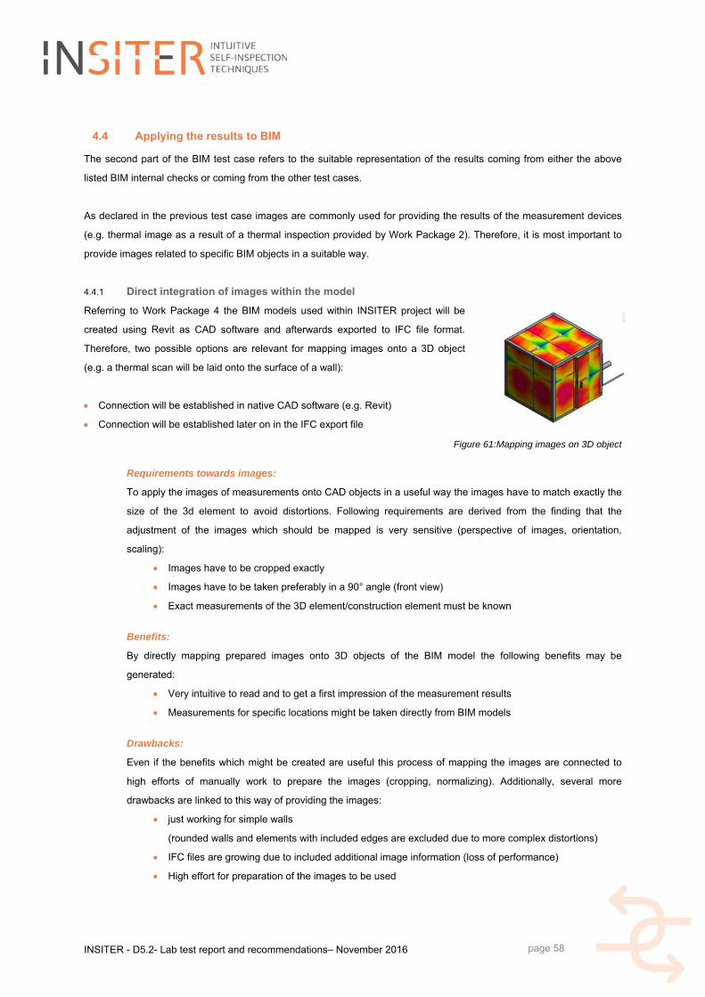
4.3.3 4D Checks 55
4.4 Applying the results to BIM 58
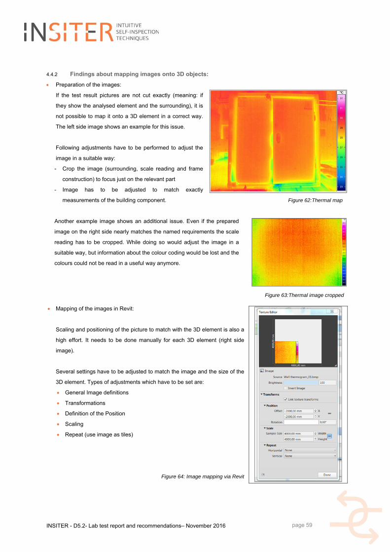
4.4.1 Direct integration of images within the model 58
INSITER - D5.2- Lab test report and recommendations– November 2016
page 8
4.4.2 Findings about mapping images onto 3D objects: 59
4.4.3 Linking of images 60
4.4.4 Colouring the model elements according to a specific value (e.g. temperature) 62
4.5 Energy Performance 64
5. TEST PLAN AND RECOMMENDATION FOR FACTORY APPLICATION 66
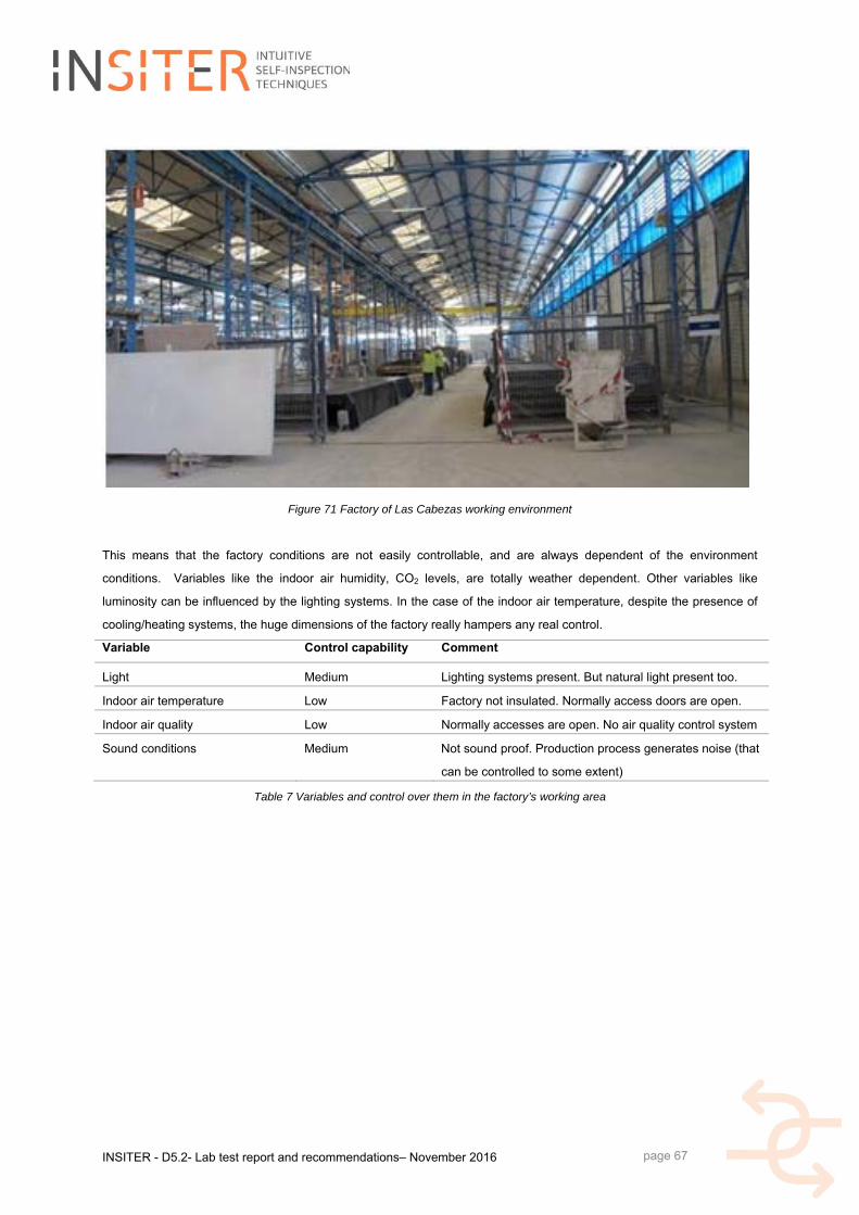
5.1 Description of Factory conditions 66
5.2 Identification of main critical issues for each test 68
5.2.1 Thermal transmittance test 68
5.2.2 Thermal bridge test 68
5.2.3 Structural integrity 69
5.2.4 General comments for this set of tests 69
5.2.5 Acoustic tests 70
5.2.6 Geometric discrepancy 72
5.2.7 Humidity 73
5.2.8 Positioning system 73
5.2.9 Data integration to BIM and AR 73
5.3 Recommendations for the tests in the factory. 73
6. CONCLUSIONS 76
7. REFERENCES 77
INSITER - D5.2- Lab test report and recommendations– November 2016
page 9
1. Introduction
1.1 Objectives and structure of this deliverable
This document is the result of Task 5.1 and its main scope is to report the lab tests performed to validate the selected
protocols described in D5.1 and the recommendation arisen in view of the application to the real test cases. The lab
tests had the aim to implement in a controlled environment the protocols and methodologies related to the INSITER self-
inspection system and to identify eventual problems that can be encountered in construction sites.
Since INSITER has defined 7 test cases (see Table 1). The test cases 4, 5, 7 have been described in D5.1 this
deliverable is focused on the remaining test cases and on test for MEP/HVAC components, based on humidity and
geometrical aspects.
Test Cases
Test case 1 Thermal test case
Test case 2 Acoustic test case
Test case 3 Air tightness test case
Test case 4 Humidity test case
Test case 5 Geometry test case
Test case 6 BIM test case and Test case
Test case 7 Augmented Reality test case
Table 1: INSITER Test Cases
Therefore, the structure of this deliverable is as following:
- Chapter 2 reports the test cases developed at laboratory level for the validation of the procedures for thermal,
acoustic and air leakage assessment (Test case 1, 2 and 3). Those tests have been performed in the cooling
room at the UNIVPM laboratory.
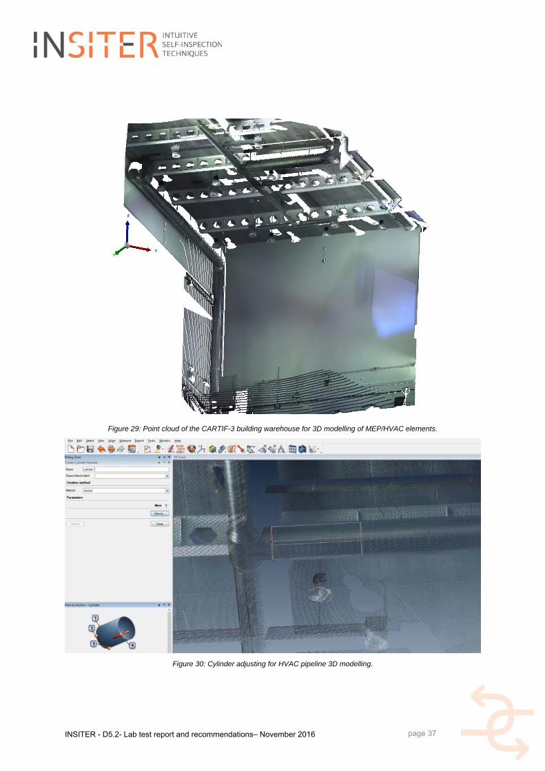
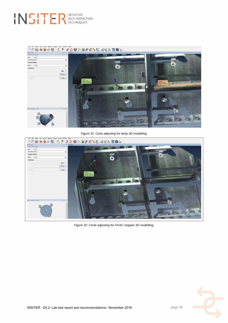
- Chapter 3 describes the use of the 3D laser scanner for the inspection of MEP/HVAC in terms of installation and
humidity performances. Those tests have been carried out by CARTIF in its CARTIF-3 Building.
- Chapter 4 illustrates how to connect experimental data to the BIM and has been developed by HOCHTIEF.
- Chapter 5 put on evidence the main recommendations for the use of the INSITER protocols in the factory.
1.2 R&D methodology employed to achieve results presented in this deliverable
This deliverable presents the main results achieved by applying diagnostic procedures identified by the INSITER project
in lab tests in order to perform a first validation in simplified test cases. The INSITER procedures have been deeply
described in the deliverables presenting the outcomes of the research performed in WP2, especially in D2.3. That
document reports the basic theory, the scientific innovation, the detailed procedure for the assessment of thermal,
acoustic, humidity, geometrical aspects that allow to monitor and diagnostic errors related to thermal transmittance of
building elements, presence of thermal bridges, structure integrity, sound transmission loss, acoustic and air leakage,
humidity and geometric gaps and/or clashes of prefab elements. The protocols related to different technologies detailed
in D2.3 have been applied in several test benches and results reported in D5.1 and D5.2.
Specifically D5.1 describes the results of:
INSITER - D5.2- Lab test report and recommendations– November 2016
page 10
- Thermal transmittance/acoustic leakage assessment of building elements,
- Thermal bridges and structural integrity identification by IR camera,
- Humidity and geometric discrepancy evaluation by 3D laser scanner in building envelopes.
Specifically D5.2 describes the results of:
- Thermal transmittance/acoustic and air leakage assessment of building envelopes,
- Thermal bridges evaluation and their quantitative affects in terms of thermal transmittance,
- Humidity and geometrics inspection in MEP/HVAC systems.
Besides, this deliverable shows some examples of experimental data connectivity to the BIM in different use case
scenarios for model 3D and 4D checks. And finally test planning and recommendation for factory tests are detailed.
1.3 Main achievements and limitations
The main goal of INSITER concerning the measurement devices is to optimize/modify/adapt standard or innovative
measurement procedures to suit the use for on-site self-inspection. Because the current procedures are either too
complex or take too much time to be applied during the construction process, INSITER has identified and developed
alternative methods for improve easiness to use and decrease the inspection time keeping a sufficient level of accuracy.
The achievement of this deliverable is the applicability of the INSITER’s innovation in lab testing thus demonstrating that
the optimized/modified measurement procedures are adequate for on-site self-inspection. After successful lab testing,
the procedures will be tested, validated and demonstrated in factory and field situation respectively.
INSITER - D5.2- Lab test report and recommendations– November 2016
page 11
2. Lab test The building quality passes through the continuous inspection of the installation process, product quality and building
performance. The techniques developed in D2.3 and protocols described in D5.1 allow evaluating the performance of
the building envelope components collecting essential data useful to:
evaluate the presence of an error/damage,
supply inputs to the self-instruction process
and, once fixed the errors if there were any, estimate energy related parameters that are sent to the INSITER
software to calculate building energy performance.
The lab tests described in this document have the aim of validating the inspection procedures for the evaluation of
thermal (Test case 1), acoustic (Test case 2) and air tightness (Test case 3) performances of the building envelope.
The same procedures have been already described in the D5.1 and validated for the evaluation of 2D components
performances, i.e. building elements (facades or partition elements). In this deliverable, those procedures have been
validated for the estimation of the 3D thermal, acoustic and air tightness performances of the entire building envelope.
As simplified test bench the cooling room available at the UNIVPM laboratory has been used.
2.1 3D thermal test
A 3D thermal test aims at the evaluation of the thermal transmittance and thermal bridges in a building envelope. The
protocols for the thermal parameters acquisition are described in D5.1 Lab test protocols and set-up, chapter 3.
The tests have been performed on the pilot test bench installed in the laboratory of the University Politecnica delle
Marche (Ancona, IT) already described in the D5.1 chapter 9. This test bench is a cooling room that can be thermally
conditioned and controlled in order to generate thermal gradients between the interior and exterior environment. The test
has been performed during the cooling of the room applied during the night.
IR thermal maps have been registered at the end of a cooling cycle of the cooling room on its four vertical walls. The
cooling cycle consisted on a cooling, by a portable cooling system installed inside the mock-up, lasting 13 hours. The
temperatures reached by the air inside and the outside the room and by the wall A, where a prefab panel supplied by
DRAGADOS was installed, (see Figure 1) are reported in Table 2.
Figure 1 Cooling room wall nomenclature
Those temperatures have been measured by thermometers placed inside and outside the room (Tin and Tout
C
A B
D
INSITER - D5.2- Lab test report and recommendations– November 2016
page 12
respectively) and by thermocouples cemented on the prefab panel interior and exterior surface (Tw,in and Tw,out
respectively). At the end of the cycle, the thermal gradient between the prefab panel internal and external surface was of
8°C and the air thermal gradient between the room interior and exterior environment was of 10°C that guarantees the
applicability of the method according to [7-1].
The humidity inside the room at the end of the cycle was 50% and outside 46%. The thermal time histories during the
cooling cycle are given in Figure 2. It can be noticed the cooling trend of both the interior (blue line of Figure 2) and
exterior environment (magenta line of Figure 2) during the night, however after 11 hours, at sunrise, the temperatures
invert the trend and start to increase. Nevertheless, the temperature gradient was still about 10°C.
Parameter Symbol Cooling start temperature [°C] Cooling end temperature [°C]
Indoor temperature Tin 28 19
Outdoor temperature Tout 31 28.9
Interior wall temperature Tw,in 28.5 20.5
Exterior wall temperature Tw,out 30.5 28
Table 2: Temperature conditions at the beginning and at the end of the cooling cycle.
Figure 2: Internal and external wall temperature time histories
The thermograms registered during the thermal cycle when the thermal camera framed the prefab panel at four time
instants are visualised in Table 3.
Frame at t= 3 min Frame at t= 60 min Frame at t= 300 min Frame at t= 740 min
Table 3: thermograms at different instants during the cooling cycle
Increasing the frame time the thermal contrast increases and the thermal bridges are more evident.
INSITER - D5.2- Lab test report and recommendations– November 2016
page 13
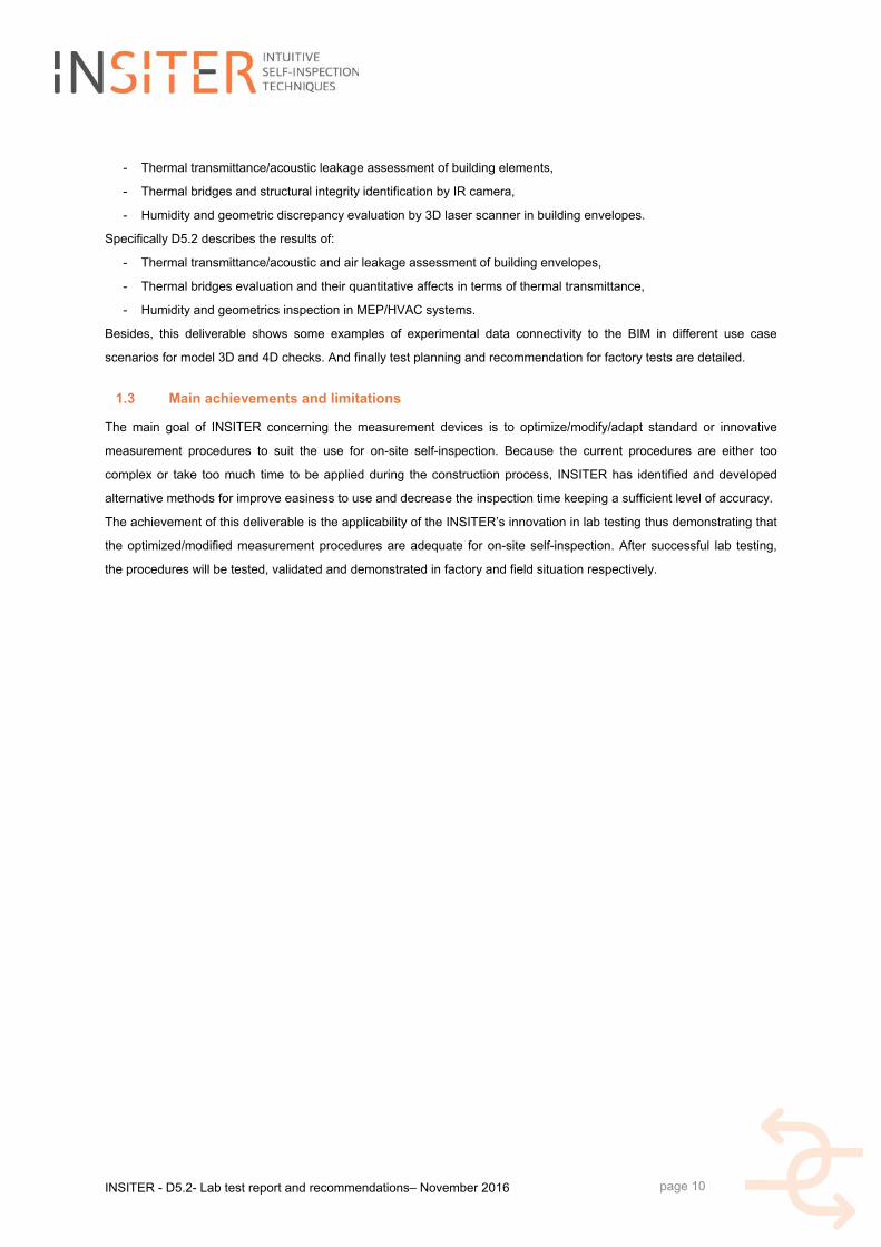
The measurement of the thermograms in the four vertical walls has been performed at the end of the cooling cycle
starting from the prefab panel (wall A) and following the sequence wall B, wall C, wall D. The complete set of
thermograms have been acquired in 20 min and during this timeframe the temperature on the wall A, internal and
external surface, varied of 1 °C, which is in the order of the thermal camera accuracy.
The thermal camera settings are summarised in
Table 4.
Table 4: Thermal camera settings
2.1.1 3D thermal maps
The thermogram acquired on the prefab wall (called wall A) georeferenced by the QR with position (0.0;220.0;1986.5) is
illustrated in Figure 3. The geo-referencing procedures are described in the D2.3 chapter 2.5. The string read on the QR
is (0.00;220.00;1986.50).
Tools and Configuration
thermal camera Infratec variocam HD
lens IR 1.0/15 LW JENOPTIK
lens position
height 1,1 [m]
distance 2,2 [m]
angulation normal
wall emissivity Panel: A Panels: B/C/D
0.97 0.98
INSITER - D5.2- Lab test report and recommendations– November 2016
page 14
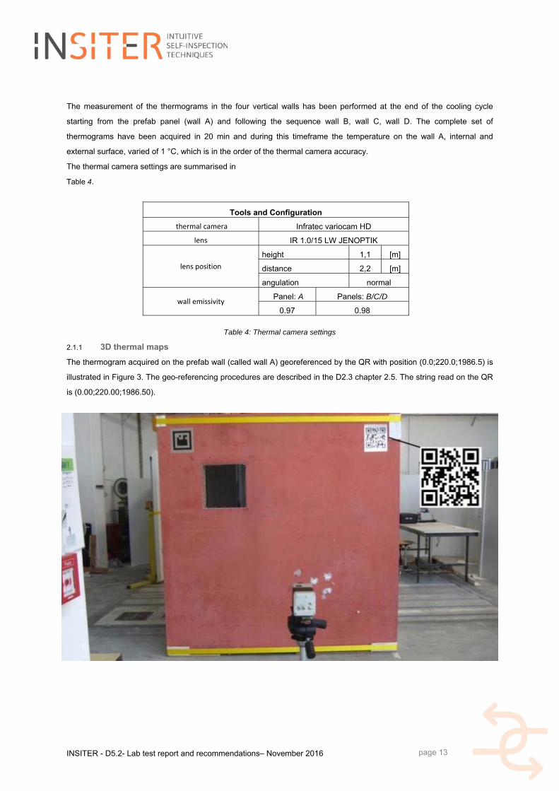
Figure 3: Wall A picture (top) and thermogram (bottom)
In Figure 3 - Figure 6 thermal cold spots are visible. They highlight areas of temperature altered by thermal bridges.
The thermogram acquired on the wall (called wall B) georeferenced by the QR with position (325.0;0.0;1986.5) is
illustrated in Figure 4. The string read on the QR is (325.00;2225.00;1986.50).
T=24,9°C T=27,5°C
INSITER - D5.2- Lab test report and recommendations– November 2016
page 15
Figure 4: Wall B picture (top) and thermogram (bottom)
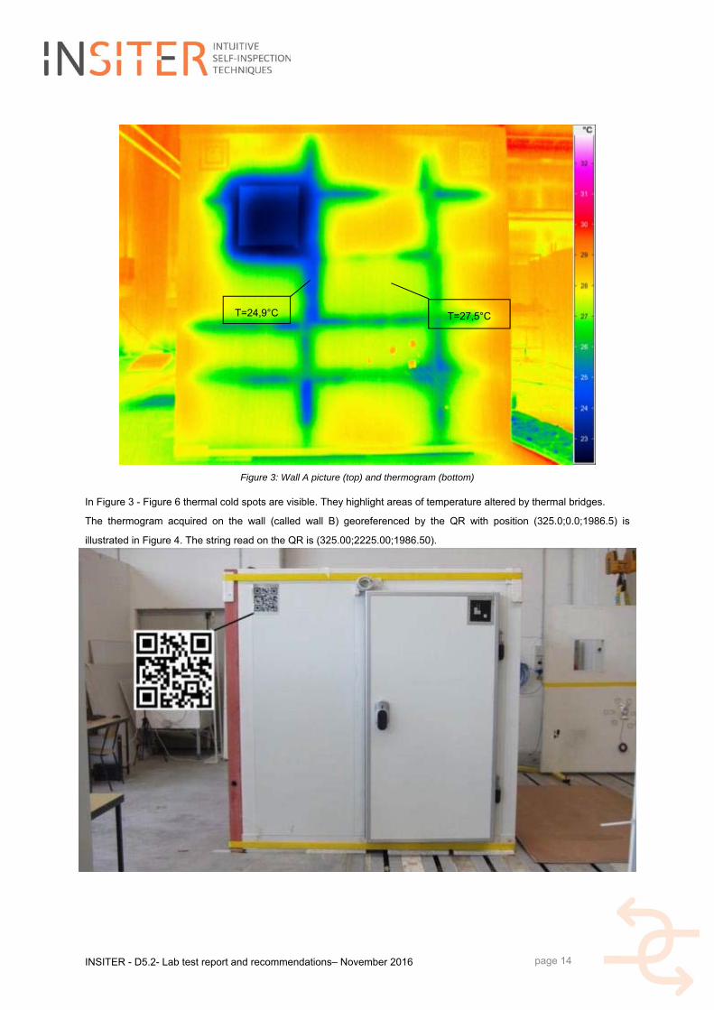
The thermogram acquired on the wall (called wall C) georeferenced by the QR with position (2346,0;2005,0;1986,5) is
illustrated in Figure 5. The string read on the QR is (2346,00;2005,00;1986,50).
T=27,1°C
T=28,5°C
INSITER - D5.2- Lab test report and recommendations– November 2016
page 16
Figure 5: Wall C picture (top) and thermogram (bottom).
The thermogram acquired on the wall (called wall C) georeferenced by the QR with position (325.0;2225.0;1986.5) is
illustrated in Figure 6. The string read on the QR is (325.00;0.00;1986.50).
T=28,5°C
T=27,1°C
INSITER - D5.2- Lab test report and recommendations– November 2016
page 17
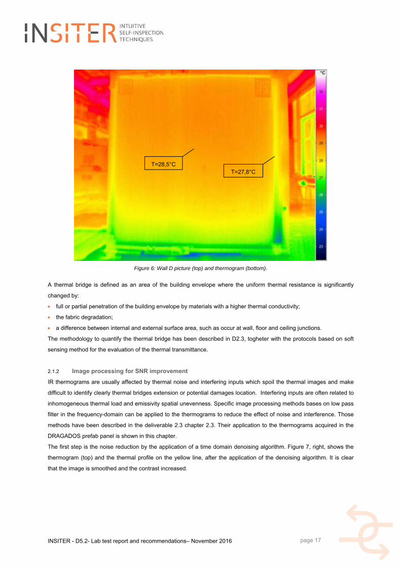
Figure 6: Wall D picture (top) and thermogram (bottom).
A thermal bridge is defined as an area of the building envelope where the uniform thermal resistance is significantly
changed by:
full or partial penetration of the building envelope by materials with a higher thermal conductivity;
the fabric degradation;
a difference between internal and external surface area, such as occur at wall, floor and ceiling junctions.
The methodology to quantify the thermal bridge has been described in D2.3, togheter with the protocols based on soft
sensing method for the evaluation of the thermal transmittance.
2.1.2 Image processing for SNR improvement
IR thermograms are usually affected by thermal noise and interfering inputs which spoil the thermal images and make
difficult to identify clearly thermal bridges extension or potential damages location. Interfering inputs are often related to
inhomogeneous thermal load and emissivity spatial unevenness. Specific image processing methods bases on low pass
filter in the frequency-domain can be applied to the thermograms to reduce the effect of noise and interference. Those
methods have been described in the deliverable 2.3 chapter 2.3. Their application to the thermograms acquired in the
DRAGADOS prefab panel is shown in this chapter.
The first step is the noise reduction by the application of a time domain denoising algorithm. Figure 7, right, shows the
thermogram (top) and the thermal profile on the yellow line, after the application of the denoising algorithm. It is clear
that the image is smoothed and the contrast increased.
T=28,5°C T=27,8°C
INSITER - D5.2- Lab test report and recommendations– November 2016
page 18
Figure 7: Left, original thermogram (top) and thermal profile on the yellow line (bottom); right, denoised thermogram (top) and denoised thermal profile on the yellow line (bottom)
To further improve the contrast between sound areas and thermal bridges the thermal contrast has been calculated as
described in D2.3 chapter 2.3. The thermal contrast is the pixel by pixel maximum contrast with respect to the sound
area evaluated in each thermal frame of the IR time history. The thermal contrast of the thermogram considered is
shown in Figure 8: the thermal bridge profile has become more evident.
Figure 8: Left, denoised thermogram; right, thermal contrast map
2.2 3D Acoustic test
This chapter presents the acoustic tests performed on the Dragados-UNIVPM mock-up. As discussed previously, the
mock-up consists of a prefabricated panel manufactured by Dragados, mounted against a mock-up room. The walls of
the room itself are correctly sealed, however the Dragados panel is placed without any special sealing in order to
replicate an incorrect installation such as that encountered in a real building scenario.
2.2.1 Experimental setup- sound intensity measurement – SoundBrush
INSITER - D5.2- Lab test report and recommendations– November 2016
page 19
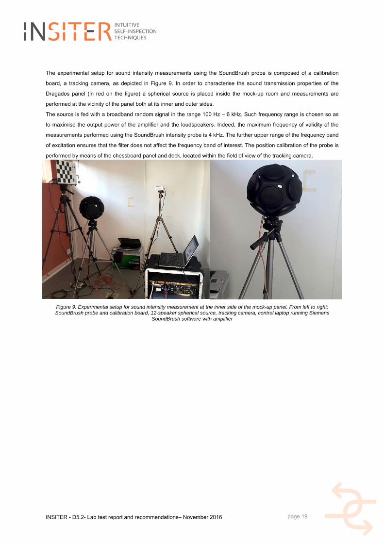
The experimental setup for sound intensity measurements using the SoundBrush probe is composed of a calibration
board, a tracking camera, as depicted in Figure 9. In order to characterise the sound transmission properties of the
Dragados panel (in red on the figure) a spherical source is placed inside the mock-up room and measurements are
performed at the vicinity of the panel both at its inner and outer sides.
The source is fed with a broadband random signal in the range 100 Hz – 6 kHz. Such frequency range is chosen so as
to maximise the output power of the amplifier and the loudspeakers. Indeed, the maximum frequency of validity of the
measurements performed using the SoundBrush intensity probe is 4 kHz. The further upper range of the frequency band
of excitation ensures that the filter does not affect the frequency band of interest. The position calibration of the probe is
performed by means of the chessboard panel and dock, located within the field of view of the tracking camera.
Figure 9: Experimental setup for sound intensity measurement at the inner side of the mock-up panel. From left to right: SoundBrush probe and calibration board, 12-speaker spherical source, tracking camera, control laptop running Siemens
SoundBrush software with amplifier
INSITER - D5.2- Lab test report and recommendations– November 2016
page 20
Figure 10: Experimental setup for sound intensity measurement at the outer side of the mock-up panel
2.2.2 Exporting SoundBrush data as a 3D model
A bash script was written in order to represent the data measured using the SoundBrush probe as a 3D model, readily
compatible with software able to import STL (stereo lithography) or X3D files.
The script outputs a JSCAD model, which is a 3D model format for the free software OpenJSCAD, which can in turn
output an STL or X3D model.
INSITER - D5.2- Lab test report and recommendations– November 2016
page 21
# 3D representation of SoundBrush measurement # Project INSITER # # This program is free software and is distributed under the terms of # the GNU General Public License, version 3 or any later version. # A copy of the license can be found here: https://www.gnu.org/licenses/gpl-3.0.en.html # # usage: # ./sb2jscad.sh <file> # <file> is a text file containing the data from any generic table # exported using the SoundBrush "Generate Report" tool # # J.Cuenca 2016 m=$(awk -v a=8 '{print $a}' i_side_nowool|sort|sed -n '1p;$p') min=$(echo $m | awk -v a=1 '{print $a}') max=$(echo $m | awk -v a=2 '{print $a}') Nl=$(more i_side_nowool|wc -l) for l in $(seq 1 4 $Nl) do awk -v line=$l -v x=5 -v y=3 -v z=4 -v phi=6 -v rho=7 -v amp=8 'NR==line {print "arrow(lx-"$x","$y","$z","$phi","$rho","$amp"),"}' $1 >> out done echo "function arrow(x,y,z,phi,rho,amp) { var res=3 var pi=3.141592 var min="$min-1", max="$max" amp=(amp-min)/(max-min) return union( cylinder({start: [0,0,0], end: [amp/10,0,0], r: 0.01*amp, fn:res}), cylinder({start: [amp/10,0,0], end: [(amp+amp/3)/10,0,0], r1: 0.02*amp, r2: 0, fn:res}) ).scale(1).rotateY(phi).rotateZ(180-rho).translate([x,y,z]).setColor([amp,1-amp,0]) } function mockup(lx,ly,lz,lw,h) { return union( cube({size: [lx,h,lz]}).setColor([.5,.5,.5]).translate([h,0,0]), cube({size: [lx,ly,h]}).setColor([.5,.5,.5]).translate([h,0,0]), cube({size: [lx,ly,h]}).setColor([.5,.5,.5]).translate([h,0,lz-h]), cube({size: [lx,h,lz]}).setColor([.5,.5,.5]).translate([h,ly-h,0]), cube({size: [h,ly,lz]}).setColor([.5,.5,.5]).translate([lx,0,0]), difference( cube({size: [h,ly,lz]}).setColor([1/2,0,0]), cube({size: [h,lw,lw]}).translate([0,ly-2*lw,lz-2*lw]) ) ) } function main() { var lx=2.53, ly= 2.38, lz=2.35, lw=.4, h=.1 return union("$(more out)" arrow(0,0,0,0,0,"$max").setColor([0,0,1]), arrow(0,0,0,0,90,"$max").setColor([1,0,0]), arrow(0,0,0,-90,0,"$max").setColor([0,1,0]), mockup(lx,ly,lz,lw,h).translate([2*h,-ly-h/2,0]) ) } " > out mv out out.jscad
Bash script for the conversion raw SoundBrush measurement data into JSCAD models
INSITER - D5.2- Lab test report and recommendations– November 2016
page 22
Figure 11: Screenshot of an example output model in OpenJSCAD, before being exported to x3d
Figure 12: Resulting x3d model of measured data visualised in MeshLab
2.2.3 Sound source localisation – acoustic array
A microphone array is employed in order to identify the sources of noise on the exterior surface of the mock-up room.
The experimental conditions are identical to those of the sound intensity measurements, allowing both acquisition
systems to operate simultaneously. The microphone array used for this test is the Siemens 2Dcam45. It is
INSITER - D5.2- Lab test report and recommendations– November 2016
page 23
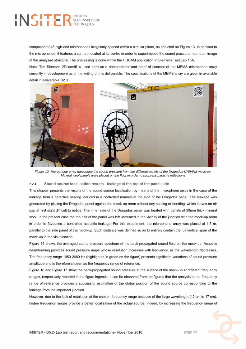
composed of 45 high-end microphones irregularly spaced within a circular plane, as depicted on Figure 13. In addition to
the microphones, it features a camera located at its centre in order to superimpose the sound pressure map to an image
of the analysed structure. The processing is done within the HDCAM application in Siemens Test.Lab 15A.
Note: The Siemens 2Dcam45 is used here as a demonstrator and proof of concept of the MEMS microphone array
currently in development as of the writing of this deliverable. The specifications of the MEMS array are given in available
detail in deliverable D2.3.
Figure 13: Microphone array measuring the sound pressure from the different panels of the Dragados-UNIVPM mock-up. Mineral wool panels were placed on the floor in order to suppress parasite reflections
2.2.4 Sound source localisation results - leakage at the top of the panel side
This chapter presents the results of the sound source localisation by means of the microphone array in the case of the
leakage from a defective sealing induced in a controlled manner at the side of the Dragados panel. The leakage was
generated by placing the Dragados panel against the mock-up room without any sealing or bonding, which leaves an air
gap at first sight difficult to notice. The inner side of the Dragados panel was treated with panels of 50mm thick mineral
wool. In the present case the top half of the panel was left untreated in the vicinity of the junction with the mock-up room
in order to favourise a controlled acoustic leakage. For this experiment, the microphone array was placed at 1.5 m,
parallel to the side panel of the mock-up. Such distance was defined so as to entirely contain the full vertical span of the
mock-up in the visualisation.
Figure 15 shows the averaged sound pressure spectrum of the back-propagated sound field on the mock-up. Acoustic
beamforming provides sound pressure maps whose resolution increases with frequency, as the wavelength decreases.
The frequency range 1950-2680 Hz (highlighted in green on the figure) presents significant variations of sound pressure
amplitude and is therefore chosen as the frequency range of reference.
Figure 16 and Figure 17 show the back-propagated sound pressure at the surface of the mock-up at different frequency
ranges, respectively reported in the figure legends. It can be observed from the figures that the analysis at the frequency
range of reference provides a successful estimation of the global position of the sound source corresponding to the
leakage from the imperfect junction.
However, due to the lack of resolution at the chosen frequency range because of the large wavelength (12 cm to 17 cm),
higher frequency ranges provide a better localisation of the actual source. Indeed, by increasing the frequency range of
INSITER - D5.2- Lab test report and recommendations– November 2016
page 24
the analysis, it can be observed that the noise source related to the leakage is in fact composed of two main areas
where the sealing is defective, radiating at different levels across the frequency range.
Figure 14: Microphone array at the side of the Dragados panel for acoustic leakage identification. Mineral wool panels were placed on the door and floor sealings in order to suppress the sources of noise originating thereupon, so as to correctly identify
the noise source due to the imperfect sealing of the Dragados panel, introduced intentionally for this test. Note: the array position in the photograph does not correspond to the final configuration
Figure 15: Averaged sound pressure spectrum on the back-propagated field at the surface of the mock-up side
INSITER - D5.2- Lab test report and recommendations– November 2016
page 25
(a) 1950-2680 Hz (b) 2830-3050 Hz
(c) 4160-4400 Hz (d) 4970-5370 Hz
Figure 16: Back-propagated sound pressure at the surface of the Dragados-UNIVPM mock-up at different frequency ranges. Top of mineral wool treatment in the inside of the mock-up removed
2.2.5 Observation of leakage across the entire panel-room junction
A second experiment was carried in order to validate the identification approach. In this case, the mineral wool was
removed from the entire vertical length of the panel’s inner side. Figure 16 to Figure 17 depict the corresponding results
at different frequency ranges. A leakage across the entire junction is identified, thus allowing for a direct correlation with
the controlled defect.
INSITER - D5.2- Lab test report and recommendations– November 2016
page 26
Figure 17: Back-propagated sound pressure at the surface of the Dragados-UNIVPM mockup at different frequency ranges. Top and bottom of mineral wool treatment in the inside of the mockup removed.
2.2.6 Sound intensity results - leakage from the panel-mock-up junction
This chapter presents the identification of acoustic leakage from the junction between the Dragados panel and the walls
of the room mock-up.
The measurement was performed in stationary conditions using a random excitation signal in the range 100 Hz – 6 kHz,
as detailed above. The frequency range of validity of the SoundBrush probe is 100 Hz – 4 kHz. The low-frequency limit
is imposed by the sensitivity of the microphones themselves and the high-frequency limit is given by the distance
between the microphones. Please refer to D2.3 for more details.
The sound pressure and particle velocity were recorded in the vicinity of the left junction of the Dragados panel with the
rest of the mock-up, in the absence of mineral wool panels in the inner side. The resulting sound intensity vector field is
represented in Figure 18. The physical gap materialises into a noticeable acoustic source, thus correctly identifying the
installation error. The acoustic power of the sound source (located inside the mock-up) was not quantified. Therefore the
INSITER - D5.2- Lab test report and recommendations– November 2016
page 27
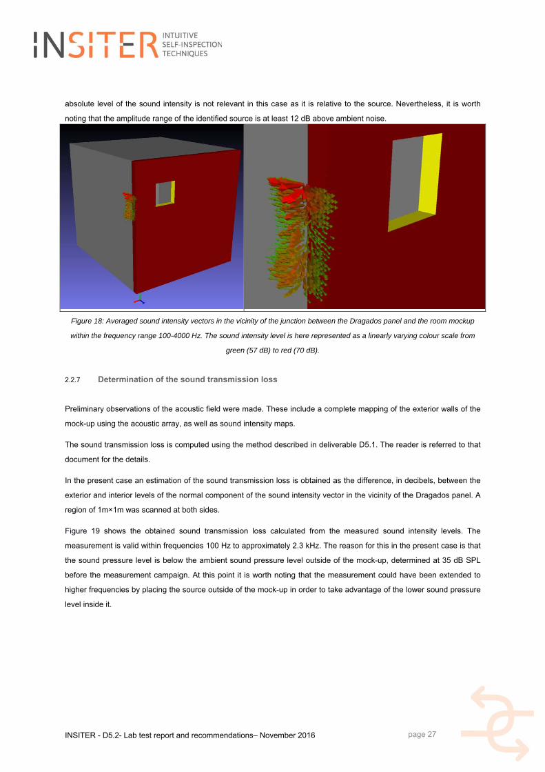
absolute level of the sound intensity is not relevant in this case as it is relative to the source. Nevertheless, it is worth
noting that the amplitude range of the identified source is at least 12 dB above ambient noise.
Figure 18: Averaged sound intensity vectors in the vicinity of the junction between the Dragados panel and the room mockup
within the frequency range 100-4000 Hz. The sound intensity level is here represented as a linearly varying colour scale from
green (57 dB) to red (70 dB).
2.2.7 Determination of the sound transmission loss
Preliminary observations of the acoustic field were made. These include a complete mapping of the exterior walls of the
mock-up using the acoustic array, as well as sound intensity maps.
The sound transmission loss is computed using the method described in deliverable D5.1. The reader is referred to that
document for the details.
In the present case an estimation of the sound transmission loss is obtained as the difference, in decibels, between the
exterior and interior levels of the normal component of the sound intensity vector in the vicinity of the Dragados panel. A
region of 1m×1m was scanned at both sides.
Figure 19 shows the obtained sound transmission loss calculated from the measured sound intensity levels. The
measurement is valid within frequencies 100 Hz to approximately 2.3 kHz. The reason for this in the present case is that
the sound pressure level is below the ambient sound pressure level outside of the mock-up, determined at 35 dB SPL
before the measurement campaign. At this point it is worth noting that the measurement could have been extended to
higher frequencies by placing the source outside of the mock-up in order to take advantage of the lower sound pressure
level inside it.
INSITER - D5.2- Lab test report and recommendations– November 2016
page 28
Figure 19: Estimation of the sound transmission loss using sound intensity measurements as described in D5.1. Left: sound intensity level at the inner (higher) and outer (lower) sides of the panel, with levels at the ensemble of measured points indicated
in grey. Right: Sound transmission loss of the Dragados panel. The validity frequency range of this particular measurement is indicated with a white background.
2.3 3D air leakage test
The air leakage detection by ultrasound system has been introduced in D5.1 chapter
10.2 as an alternative for the measurement of the air tightness performance of the
building envelope. This is a very promising method to detect leak on open and close
structures thanks to the small wavelength used. The theoretical aspects and protocols
for calibration and testing have been detailed in the D2.3, chapter 7. In this chapter,
the results of the inspection by ultrasound system on the cooling room where the
DRAGADOS prefab panel is installed (Figure 3) are described. The air leakage
detection requires the generation of ultrasound waves (frequency range between 30
and 50 kHz) inside the close envelope and the acquisition of the transmitted waves
outside the envelop.
In this case the ultrasound waves have been generated by an air blow gun placed
inside the cooling room and directed towards the prefab panel (Figure 20). The
pressure level has been set at 2.5 bar.
Figure 20: air blow gun placed inside the cooling room.
The ultrasonic receiver (Ultrasonic Detector SDT 150) is placed outside the cooling room (Figure 21, left) and is
connected to an digital acquisition board installed (acquisition board NI PXI- 5122) to a PC for recording data measured
while the operator scans the area along the junction between the prefab panel and the cooling room structure. The
ultrasonic receiver was kept about 2 cm away from the wall by the operator. The scanning spatial resolution was of 5 cm
in the vertical direction The acquisition rate has been set at 1 MHz and RMS (Root Mean Square) value of the time
signal was calculated every 2 ms interval. The operator was scanning the junction at approximately 12 mm/s speed so
that the acquisition system acquires more than 40 samples per mm, i.e. the probe moves of 1mm in 83 ms.
INSITER - D5.2- Lab test report and recommendations– November 2016
page 29
Figure 21: Ultrasound detector connected to pc (left), scanning area by operator (right).
The RMS ultrasonic level in Volts measured over the scanned are illustrated in the following figures for the different walls
of the cooling room. Figure 22 (left) highlights a small leak on the window frame that is identified also by the ultrasonic
level map, because the leak allows the ultrasonic waves to be transmitted to the exterior. An increase of the ultrasonic
RMS level is evident in the ultrasonic map shown in Figure 22, right.
Figure 22: DRAGADOS panel (Wall A ), left; Ultrasonic level map, right.
Figure 23 shows the scan area on the wall B and the map highlights a leak along the junction between the prefabricated
panel and the cooling room structure. Moreover a small leak appears also on the bottom of the door probably due to a
problem with the sealing.
Figure 23: Wall B , left; Ultrasonic level map, right.
Ultrasound detector
INSITER - D5.2- Lab test report and recommendations– November 2016
page 30
Figure 24 shows the scan area on the wall D, also in this case a leak has been highlighted corresponding to the junction
between the prefab panel and the cooling room structure, as expected.
Figure 24 Wall D, left; Ultrasonic level map, right.
Figure 25 shows the scan area on the wall C, in this case any leak has been detected.
Figure 25 Wall C, left; Ultrasonic level map, right
2.4 Comparative overview of the achievements
Chapter 2.4 presented the applicability of the INSITER diagnostic tools for different measurement aspects assessment.
Hereafter the main advantages/disadvantages of those techniques with respect to the currently available are
summarised in terms of the measurement aspects addressed.
Concerning the thermal transmittance the IR camera based soft sensing procedure allows to reducing the testing time by
keeping the same level of accuracy. The current standard for in-situ thermal transmittance measurement by means of
heat flow meter (ISO 9869) states that the U-value can be evaluated with an accuracy of about 8%, depending on the
environmental conditions. The inspection time is a function of the building element thermal phase (or time shift related to
its thermal inertia) and is influenced by the stability of the natural day cycle. The standard, in fact, is based on natural
day cycles for the generation of a gradient between the internal and external surface of the building element. The
minimal inspection time declared is of 72 h but the test can be stopped only if the U-value do not change more than 5%
for three consecutive nights. Standard testing time is between 7 and 15 days. The IR camera soft-sensing method
proposed as INSITER thermal transmittance measurement system is based on forced thermal cycles and an
INSITER - D5.2- Lab test report and recommendations– November 2016
page 31
accompanying model which allows to decrease the testing time up to some cycles (between 20 and 60 hours) depending
on the thermal phase of the building element (4 h for a concrete wall or 10 h for an high insulation wall, respectively).
The cost of the equipment used in the current standard (ISO 9869) is of about 3000€ (cost of the heat flow meter) even
though is strongly suggested to use an IR thermal camera to accurately position the heat flow meter on an region free of
thermal bridges. The cost of the thermal transmittance tools proposed by INSITER is of about 5000€ (cost of the thermal
camera). The same tool proposed by INSITER for the thermal transmittance evaluation (IR camera) is used for thermal
bridge estimation and quantitative effect estimation on the global transmittance. The current standard ISO 14683 allow
estimating the linear thermal transmittance of thermal bridges in building construction by numerical calculation. The
INSITER procedure is based instead on real measurements.
Concerning the acoustic aspect the tools proposed by INSITER are the SoundBrush and the acoustic beamforming for
acoustic leakages identification. The first has the main advantage of having installed a tracking device able to localize
the measurement position in relation to the testing element. The positioning system has been interfaced with the BIM in
order to easily superimpose the measurement data to the 3D model. Beamforming also called acoustic camera is
powerful tool since, as the name states, allows visualising acoustic fields and therefore localising sound insulation losses
or acoustic leaks, superimposing them onto the visual image of the building component.
Finally, the method proposed as INSITER tool for air leakages localisation is an improvement of the current standard
based on blower door test (EN ISO 9972) which allows only to assess if air leakages are present but not to identify their
spatial position. INSITER proposes to use ultrasound probes to localise in spade air leakages of approximately 3-20 mm
width. Only with sensors working in the ultrasonic frequency range (20-100 kHz), it is possible to identify such tiny cracks
thanks to the small wavelength of the ultrasonic waves. For bigger cracks or gaps between building elements the tools
proposed by INISTER for acoustic aspects assessment can be applied indifferently. Since they are working on a
frequency range up to 10 kHz they are suitable for the detection of gaps larger than about 30 mm.
Table 5 summarises the main characteristics and innovation of the INSITER tools for acoustic/thermal/air tightness
aspects assessment.
Meas. Area
Main characteristics Innovation for on-site self-inspection during construction and maintenance
Addressedchallenges for on-site
use
Conventional procedures
INSITER procedures Accuracy Testing
Time Cost User-
friendliness
Thermal transmittance
ISO 9869 In-situ measurement of thermal resistance and thermal transmittance -- Part 1: Heat flow meter method
IR thermal camera measurement method accompanied by a numerical model of the building element (Soft Sensing based IR camera)
5% lower than current standard (8%)
Up to 50% of reduction with respect to the current standards depending on the thermal properties of the building elements and environmental stability
5000 € Higher than heat flow meter but IR camera is used also for thermal bridge assess-ment
IR camera is a non-contact measure-ment system, that simplify its application in field
Environ-mental conditions variation
Thermal load application
INSITER - D5.2- Lab test report and recommendations– November 2016
page 32
Thermal bridge
ISO 14683 - Thermal bridges in building construction -Numerical calculation
IR thermal camera based method for the evaluation of thermal bridge influence on building element global transmittance
5% in line with the numerical model method
Increased time required for experimental data acquisition
5000 € The IR camera is used also for thermal transmit-tance assess-ment
IR camera is a non-contact measure-ment system, that simplify its application in field
Environ-mental conditions variation
Thermal load application
Acoustic test
Sound level meter - ISO 16032:2004
Sound pressure level by Beamforming microphone array
Spatial leak detection in the order of 10 cm
Lower that 10 min for an area of 200 cm x 200 cm
Higher than a sound level meter
The acoustic field distribution is automati-cally superimposed to the visual image of the building component
Environmental conditions variation
Intensity probe - ISO-9614 series
Sound intensity field by SoundBrush
Spatial leak detection in the order of 30 mm
About one hour for an area of 200 cm x 200 cm
Higher than a sound intensity probe
The position of the measurement point is automatically recorded by a tracking system
Environmental conditions variation
3D Air leakage test
EN ISO 9972 -Blower door test
Ultrasonic waves detection
Spatial leak detection in the order of 3-20 mm
About one hour for an area of 200 cm x 200 cm
3000 euro
Similar to Blower door equipment
The ultrasonic probe is manually moved and its position tracked by automatic positioning system as the SoundBrush one
Noise in the ultrasound range
Table 5: Comparative overview of the achievements
INSITER - D5.2- Lab test report and recommendations– November 2016
page 33
3. Inspection & Instruction information for
MEP/HVAC installations
MEP (Mechanical Electrical and Plumbing), in addition to HVAC (Heating, Ventilating, and Air Conditioning) equipment is
often crammed into a much awarded shaped space in energy-efficient buildings made of prefab components. This is the
case of CARTIF-3 Building (INSITER Spanish demonstrator), according to:
Project setting: Building maintenance
Test case 4: Humidity
Test case 5: Geometry
Digital surveys carried out laser scanning and modelling of representative MEP/HVAC elements. A LEICA HDS-3000
was used, trying to evade voids (2cm @ 7m). Once X, Y, Z and L data were saved in Cyclone, they were registered
together into PolyWorks universal reverse engineering and inspection software [http://www.innovmetric.com].
The automatic guidance for extracting the bulk of the piping and other interesting features was done in PolyWorks
(cylinder, cones, planes, rectangles, circles) and transferred into CAD/BIM for manual completion and to clean up,
adding elbows and fixing any areas the scanner could not pick up.
The final deliverable is a MEP/HVAC model with all elements correctly represented, useful to the MEP/HVAC engineers
to identify the supply work, possible leakages and begin the maintenance actions with the aim of mitigating any clashes
or nasty surprises on site.
3.1 Use of 3D reflectivity information for MEP/HVAC inspection and instruction
The index of reflectivity (L) was processed according to the protocol for humidity check related on D5.1. This protocol
indicates the guidelines that an operator should follow for self-instruction on this purpose.
The practical demonstration of the utility of this type of data for the inspection & detection of moisture, with a real
example in one HVAC system of the Spanish demonstrator (CARTIF-3 building), has already been made in the chapter
5 of the D2.3. Therefore the repetition of procedures here is avoided.
As additional application, now the technique is directed to a MEP system in CARTIF-3. After the digitization of the
workshop area in that building (Figure 26) a higher resolution is just used on the MEP system (2mm @ 14m: Figure 27).
The result is seen in Figure 28, where humidity is not evident, but the elements of the system and the types of material
are distinguished.
INSITER - D5.2- Lab test report and recommendations– November 2016
page 34
Figure 26: Recording of the index of reflectivity in the workshop area of CARTIF-3.
Figure 27: High-res 3D scanning (dotted square) of the MEP system example in the workshop area of CARTIF-3.
INSITER - D5.2- Lab test report and recommendations– November 2016
page 35
Figure 28: Dense point cloud (up) of digitized MEP system (down).
INSITER - D5.2- Lab test report and recommendations– November 2016
page 36
3.2 Use of 3D geometric information for MEP/HVAC inspection and instruction
Increasingly MEP/HVAC contractors involved in renovation and/or refit projects are looking for solutions that will enable
them to quickly and effectively digitally represent the as-built environment as a 3D CAD/BIM model.
The emphasis with CAD/BIM is usually on the upstream activities: specification, design and build activities primarily for
the construction of new buildings. More recently, MEP/HVAC contractors have begun to enthusiastically embrace the
use of “Field to CAD/BIM” technologies like 3D scanning, seeing the benefits of using these tools in the design and
modification of existing buildings. The goal is the transfer of as-built building information from point of source in the field
directly into a CAD/BIM.
Using 3D scanners in combination with software to process and analyse the generated 3D point clouds and create a
CAD/BIM is much faster and creates a better quality and accurate/precise solution than manual measurement and
drawing techniques. 3D scanners are getting easier and easier to use, meaning inexperienced users can be trained to
scan a site very quickly, avoiding experienced staff for days measuring and creating 2D drawings or 3D models.
Moreover 3D scanners are currently relatively inexpensive given the quality of the data produced and the speed and
ease of data capture. MEP/HVAC contractors are provided with a greater understanding of the as-built environment
regarding the usual manual measuring procedures. This can lead to a reduction of clash and general errors caused by
omissions and manual mistakes made during the measurement and drawing process. Hence, creating a 3D CAD/BIM
model using scanning methods is a two stage process:
Firstly scanning the site to create a point cloud (millimetrical accuracy).
Secondly analysing and processing the point cloud and produce a 3D model.
Many contractors wrongly think that the majority of the work is done during the 3D scanning phase, but this is not the
case. As we already know, 3D scanners create point clouds. These point clouds must be turned into the CAD/BIM
models as output using processing software. The quality of the models and the speed to produce them will be dependent
in part on the selection of high quality point cloud processing and analysis software. There are two ways of producing a
useful CAD/BIM model from point clouds:
Just directly modelling into the CAD/BIM tool by means of special plug-ins, as stated for the REVIT case in the
D5.1, chapter 9.2.3.
Just using specific software tools for 3D modelling that allow the creation of parametric elements to be
exportable to CAD/BIM environments further on.
Let’s focus on this last case since has not been contemplated in any other deliverable. Thus, some representative
examples of MEP/HVAC modelling by means of PolyWorks (IMInspect module) using CARTIF-3’s workshop data are
presented here. The model is built up manually by repeatedly selecting sets of points from the point cloud that
correspond to individual 3D elements and then converting them to geometry (Figure 29). The selection needs to contain
all the points that are relevant to the geometry that is going to be created (Cylinder: Figure 30; Cone: Figure 31: Circle:
Figure 32; Plane: Figure 33).
INSITER - D5.2- Lab test report and recommendations– November 2016
page 37
Figure 29: Point cloud of the CARTIF-3 building warehouse for 3D modelling of MEP/HVAC elements.
Figure 30: Cylinder adjusting for HVAC pipeline 3D modelling.
INSITER - D5.2- Lab test report and recommendations– November 2016
page 38
Figure 31: Cone adjusting for lamp 3D modelling.
Figure 32: Circle adjusting for HVAC stopper 3D modelling.
INSITER - D5.2- Lab test report and recommendations– November 2016
page 39
Figure 33: Plane adjusting for MEP wireway 3D modelling.
The tools within the point cloud modelling software allow building up the geometry for each item as much as
automatically as possible. This activity is repeated until all required elements of the building are modelled (Figure 34). In
addition any kind of measuring verification and dimensioning can be carried out on the point cloud and on the obtained
parametric features (Figure 35).
INSITER - D5.2- Lab test report and recommendations– November 2016
page 40
Figure 34: Basic modelling of MEP / HVAC representative elements.
INSITER - D5.2- Lab test report and recommendations– November 2016
page 41
Figure 35: Distance and angle measuring on the MEP point cloud.
Good point cloud modelling software will contain functionality that allows duplicating geometry across the model,
meaning that is only needed to model repeated items once. Additionally, it could also contain tools that speed up the
creation of common MEP/HVAC items (this is the case of well-known software such as: TRIMBLE RealWorks
[http://www.trimble.com/3d-laser-scanning/realworks.aspx] or the LEICA CloudWorx family [http://leica-
geosystems.com/products/laser-scanners/software/leica-cloudworx] that allows you to automatically model a pipe by
selecting a section of the pipe data in the point cloud and then extrude the section along the point cloud. The extract
function will create a pipe that follows bends in the point cloud (Figure 36).
INSITER - D5.2- Lab test report and recommendations– November 2016
page 42
Figure 36: Plant modelling using LEICA Cyclone 9 [Source: C.R.Kennedy & Company].
As final step, CAD/BIM models are generated from 3D scanning by exporting the modelled features to useful formats
(Figure 37). Hence the global described process implies reduction of cost of model creation, deskilling of model
generation activities, budget reduction and quality improvements.
Figure 37: Exporting to IGES format of a modelled pipeline (valid for CAD and BIM).
INSITER - D5.2- Lab test report and recommendations– November 2016
page 43
4. Virtual/Real testing of quality and performance
levels based on BIM
4.1 Prove models to guarantee smooth BIM processes
Since the BIM model represents a crucial part of INSITER project regarding information and documents provided via 3d
elements, it is essential to guarantee proper workflows based on BIM. The most common errors occur due to misspelled
attribute namings and wrong formats of entered values. To prevent those errors the BIM model has to be evaluated
regarding specific rules depending on the processes they are used for.
This chapter is referring to test case 6: BIM. The test case is for validating the consistency of the BIM models
considering the aimed processes.
4.1.1 Model checks -> processes (naming conventions, data availability, attributes)
To guarantee smooth processes related to the BIM models it is important to use naming conventions. This will assure
that the BIM models and connected information can be addressed in an automated way. Testing the functionality of
automated model checks is the key to setup stable workflows and processes.
4.1.2 Deviation analysis -> Augmented Reality (geometrical exactness)
For using the technology of Augmented Reality it is most important to use BIM models consisting of very exact
geometrical data. Therefore, techniques have to be validated to guarantee that the created BIM models match the reality
even if available 2D drawings (input information) are very poor quality. Deviation analysis between created models and
available laser scan information is the key to validate the BIM models regarding geometrical correctness.
4.1.3 4D checks -> sequences (logical correctness of time schedules)
Using 4D simulations will offer the users a great opportunity to check the construction sequence for logical errors (e.g.
columns will be created prior to the pouring of the below slab is finished). Therefore, it has to be tested how to
communicate detected issues which are 4D related.
4.2 Validate the representation of results created by the other test cases
This part of the BIM test case is for approving the ability to provide results from the measurement devices to the project
team.
4.2.1 Provide data via BIM (additional documents, attribute values, links)
To prove that results coming from several measurement devices may be attached to a BIM model in a suitable
way the functionality of providing the information has to be tested. It has to be validated that external data (like
documents and drawings), external links (to several internet sites) and values of BIM attributes (e.g. specific
INSITER - D5.2- Lab test report and recommendations– November 2016
page 44
value added to an attribute) can be provided to the project team.
4.2.2 Provide model check results (Feedback on model analysis)
In case model checks can be performed in a feasible way the results of such an analysis must be provided to
the project team. This part of the test case investigates the possibilities on how to forward the identified issues
of model checks.
4.2.3 Results of a deviation analysis(Feedback on geometrical exactness)
Results of a deviation analysis must be provided to the creator of 3D models to enable them to update their
models if necessary. This part of the BIM test case refers to providing results of a deviation analysis.
4.3 Use Case Scenario Examples
Since currently the necessary requirements are not finally decided yet a fictional project has been used to approach the
model checking. Several common checks have been setup and tested to easily transfer them later on to the INSITER
use cases.
4.3.1 Model Checks
Model Checks are relevant if it comes to quality management regarding BIM models and related processes. To
be able to ensure the correctness of the used models regarding available attributes, geometrical consistence
and included information is the key to guarantee that no errors occur in further processing or at least keep
them at a very low level.
To keep the model checking system open to be able to enhance the INSITER toolset by adding additional and
more complex checking rules the decision was to use Desite MD for model checking. This software provides
an API which gives the possibility to address the BIM models from outside of the checking software as well as
to export information for further processing.
Figure 38: API (application programming interface) of Desite MD to setup model checking system.
INSITER - D5.2- Lab test report and recommendations– November 2016
page 45
Additionally, it is possible to enhance the functions of the software by including user-defined properties (to have the
possibility to enhance queries) and to include scripting functionalities in case more complex model checks have to be
setup.
Figure 39: user-defined properties in Desite MD
Even if there are several kinds of Model Checks available all of them are going through the same process.
Preparation Checking Results
Preparation First, the models to be checked have to be loaded to a model checking software and all
objects which should be analysed have to be selected for performing a specific check. This
definition of to be checked elements might become relevant if only a specific area should be
analysed.
INSITER - D5.2- Lab test report and recommendations– November 2016
page 46
Figure 40: The GUI (graphical user interface) of Desite MD
Checking Before starting the model check itself pre-conditions have to match. Defining pre-conditions
enable the model checker to reduce the selected objects to just the relevant objects for a
specific check. For example, a check about “used concrete” is irrelevant for door objects.
Figure 41: Preconditions and Attribute Rules
Pre-conditions and model checks are defined in the same way. It has to be defined which
attribute of the selected 3D models has to be addressed and of which type this specific
attribute has been declared (e.g. string, number, link). This guarantees that the check is
referring to the correct value. In case the given value of an attribute does not match the
named type or the attribute is not available for the 3D element the check would give a
“warning”. Therefore, it has to be defined how this case has to be interpreted (failed or
correct). The checking rule itself concludes the main process of checking where it is stated
which statement has to be true to fulfil the model check.
Depending of the allowed values for a model check and the type of the attribute the
checking rule will be setup differently. It is possible to use logical operators directly in the
definition of the allowed values (e.g. “>” value must be larger than) or to include several
INSITER - D5.2- Lab test report and recommendations– November 2016
page 47
different allowed values “e.g. value must be “RL” or “TL” or “SL” or “ZZ”). In case the allowed
values are a list of many entries it is possible to list them in an Excel-sheet. This list may be
referenced to check the attributes against lots of values as well.
Some examples for possible model checks are listed in the following image:
Figure 42: Model checks examples
Results After performing the model checks, the results will be analysed and reports will be created
for further processing.
Figure 43: Model checks report
On one hand the results will be listed in the checks themselves, on the other hand the 3D
component also provides the possibility to analyse the results.
Figure 44: Highlighting the model check results in 3D
INSITER - D5.2- Lab test report and recommendations– November 2016
page 48
The colour coding enables the model checker to highlight all correct and wrong elements as
well as those with a warning (e.g. the 3D element contains not the referenced attribute and
therefore the specific check might not be performed).
To provide the evaluated results to the project team there are several options for transferring
the findings. Beside analysing directly in the model checking tool there are the options to
forward the results to a connected database or the export them into an Excel-sheet for
further processing.
Figure 45: Report alternatives: Database & Excel
All of the available types of model checks follow the above mentioned process: attribute-
checks, contact-checks, geometry-checks and ID-checks as well as the comparison of the
different versions of models. All those mentioned kinds of checks will be explained below.
Figure 46:Types of model checks.
Attributes Check
The most complex check is the attribute check which gives the model checker
the most options due to the fact that available attributes may be enhanced by
scripts and user defined properties can be added.
INSITER - D5.2- Lab test report and recommendations– November 2016
page 49
For setting up the model checks it is essential that all
3D elements in the model have all necessary
attributes. Creating a list of attributes is a helpful way
to enable the modelling team to prove if all necessary
data is included in the 3d model (right side image).
All those attribute should be accessible in the 3D
model as well.
Figure 47: 3D elements and attributes
All these parameters will also be transferred by exporting the IFC file from the CAD system.
On the other side it is most important to know exactly the allowed values for a specific check. All kinds of input
values may be checked, but must be considered while setting up the different model checks. This might be an
Excel sheet with listings of allowed values as well as a table in a database. While setting up the different model
checks information about the way how the allowed values are given is essential.
To summarize the findings regarding model checks, there are two important issues which must be covered
before starting to create model checks and analyse their results. On one hand the range of allowed values
must be considered (must be provided via lists or database entries) and on the other hand there must be
information about the current situation available which should be evaluated (e.g. measurement results of
inspections, attributes of 3D elements).
Bringing both sides together enables the model checker to validate the BIM models and forward results to the
project team for further processing.
Example: Approval of Name Definitions
To standardize the modelling process, it is important to define a naming convention, which clearly defines the
naming of files and elements (families/types/layers/elements itself/attributes) as explained by Work Package 4.
Creating attribute checks may be used for the approval of the correct naming convention used for a 3D model.
It is possible to evaluate the complete naming or just specific parts of the naming (this might be necessary if a
defined substructure is defined within the naming convention).
Example: Links and additional data checks
Due to the fact that there is a lot of additional information which needs to be added to a 3D model element,
INSITER - D5.2- Lab test report and recommendations– November 2016
page 50
(e.g. test results, pictures, links, additional data) it is necessary to approve the given links. It is possible to
evaluate if a specific data is correctly attached to the model and additionally it can be checked if the value
given in the model matches with given values in a test report for example. Data consistency may be approved
this way.
Geometrical consistency check
Another important check, especially if quantity take-off is needed in the
project, is to analyse if the 3D elements are closed solids. Unfortunately it
often happens that some elements are not properly exported from CAD
system to IFC format. This may result in that those mismatched elements have no volume due to the fact that
the elements are not closed solids. Therefore, those elements cannot be used for meaningful quantity take-off
anymore. A check run which shows results of the consistence of the 3D elements is a very helpful tool to avoid
such corrupt data.
Figure 48: Example for a Geometrical Consistency Check
Unique ID Check
Having a unique ID for each model element is crucial to avoid any kind of
mismatch in the evaluation of all data. Therefore, a check may be setup to
evaluate whether all used IDs of all 3D elements are unique to avoid wrong
addressing. Otherwise wrong addressing could lead to corrupt BIM
processes.
Contact Check
The contact check verifies contact of adjacent elements (for example: are
structural walls directly connected to the slab below?). This kind of model
check is also very important for checking the correctness of room models
which are the required input data for energy simulations via VABI element
INSITER - D5.2- Lab test report and recommendations– November 2016
page 51
(see 4.5). In case that the given room elements do not fit to the existing walls
it is not possible to perform a meaningful energy calculation.
Version checking
The comparison between different versions of BIM models is slightly different to the other model checks due to
the fact that two models have to be loaded previously before performing this check. The version checking will
be used to identify all changes between model updates (deleted, changed and new 3D objects as well as
attributes). The most important aim of this check is to keep track of the design changes and to verify model
revisions.
Figure 49:Version checking
4.3.2 Deviation analysis
To be able to use the BIM models for augmented reality it is most important to match the given construction
situation on site with the BIM models appearance. To get reliable results with the BIM models even if only poor
2D data is available to create 3D models deviation analysis will be performed to compare laser scanning point
clouds with created BIM models.
To test the deviation analysis, the project of the Pisa school complex has been used. Starting point were
several 2D drawings with only some information for creating BIM models on one hand and on the other hand
there were 26 point clouds of performed laser scans.
The deviation analysis was tested with the software “Scan to BIM”. For the test the 3D-model of the School
Complex Pisa provided by Work Package 4 was used. “Scan to BIM” was chosen for the deviation analysis,
because the 3D model is a Revit model and the point clouds were submitted in the ReCap format.
INSITER - D5.2- Lab test report and recommendations– November 2016
page 52
“Scan to BIM” is a plug-in for Revit. This software has the following functionalities:
Assist the creation of Revit objects
- Automated creation of Walls, Topology, Curtain Walls, Pipe, Duct, Conduit and more.
- Construction geometry to assist with placement and creation for other object types
Workflow-based tools to help set up and work on your model with the point cloud
Measure points within your scan to quickly find true dimensions
Tools to compare what was modelled against the point cloud for visualizing and documenting deviations.
At the beginning of the test there was the problem that the point cloud and the 3D model had different
coordinates. So that the point cloud and the 3D model did not have the same location. There are three different
options to load the point cloud in Revit, but in every option the result was that the location does not match
between point cloud and 3D model.
Figure 50: Coordinates of point cloud and 3D-model doesn´t match
After the import the point cloud needs to be aligned manually to the 3D model by moving and rotation.
Figure 51: Aligned point cloud
The deviation tool in “Scan to BIM” is a visual inspection tool. It should show the deviation/difference between
the point cloud and the 3D model. The tool uses planar and curved surfaces for the analysis. Points will be
coloured based on their distance to the geometry. Colours and distances are defined on the “Point Cloud
Distance Style”. The style can be adjusted according to the project relevant settings.
INSITER - D5.2- Lab test report and recommendations– November 2016
page 53
Figure 52: Adjustment of deviation style
There are two different ways of how to do the deviation analysis in “Scan to BIM”:
Pick faces
That means that only one face of an element can be checked. In the demo project one face of the facade
was checked. In the result only the points which are located directly at the face will be coloured with the
defined style. There is a distance of max. 2 cm in the result.
Figure 53: Result of deviation analysis by "pick face" method
Element based
In this case the elements that should be checked have to be selected. With this method it is possible to
check more than a single element.
Figure 54: Elements shown in blue are selected for the deviation analysis.
INSITER - D5.2- Lab test report and recommendations– November 2016
page 54
Figure 55: Result of the deviation with the Element-Based method
Reporting of results:
There is the possibility to save views with deviation results. With the option "File + Export + Image" it is possible
to export the result to an external file or just only do a right click in the current view and choose "Save Project As
Image" - this will put the image in a rendering view type.
Findings about deviation analysis
It is necessary that the point cloud and the 3D model are having the same coordinates, because to align the
point cloud to the model will bring errors in the results. Obviously in the first deviation picture (Pick Face
Method) there is a negative and positive value of coloured points. This might be, because of the manual
rotation of the point cloud to the model.
The "Scan to BIM" tool is good when working with Revit, because it is possible to save views with marked
errors. The advantage of saving the view in Revit with marked errors are:
- it allows the team to quickly identify where the error is,
- it saves time in creating the views required for updating the error,
- it enables easy comparison of revised updates of the models by overlapping the views in Revit,
Deviation analysis will be carried out selectively – either by zones, rooms or by element types depending on
the project requirements.
For elements whose geometry is directly in contact with laser scan (which are not hidden by
finishes/insulation/other elements), deviation analysis will be done using “Scan to BIM” plug-in for Revit and the
errors will be marked in saved Revit views. The colours of the points in the view will indicate the deviations
along the element being inspected.
Some elements may have finishes such plaster, cladding. If these finishes are not modelled there may be false
deviations with laser scans. If the tolerance cannot be generalized sections in Revit will be produced that will
be analysed manually through visual checks by a BIM specialist. The deviations will be marked with revision
clouds and saved as Revit views.
In the case of using the face-based comparison negative values will indicate that the distance is behind the
face (rather than in front of it). In both cases the application will determine the bounding box of the geometry
and query the points from the point cloud that surround this data.
For working with “Scan to BIM” it is necessary to convert the point cloud in the ReCap format, because Revit
can only load these kind of files. The process of the transformation needs a long time (depends also on the
size of the project, but this process might take some hours).
The results of the two mechanism to generate the deviation analysis are different, because:
- Deviation Analysis by picking faces: All points behind and in front of the face will be coloured. Therefore,
INSITER - D5.2- Lab test report and recommendations– November 2016
page 55
negative values are possible as well. This method is only suitable for small projects (or if a single surface
should be evaluated).
For example: to check one rectangular column four analyses are required to proof the outer surfaces. For
bigger projects this way of checking is too time consuming to be suitable.
- Deviation analysis by selecting model elements: In this case only positive values will be coloured in the point
cloud. With this method it has to be considered in advance precisely what is tested. When selecting many 3D
elements of a project at once the process of the analysis may endure a long time due to many calculations.
For this reason, it is recommended to divide the model for analysis – either according to specific areas or
element types.
For this test case just nine elements were selected and the tool needed for the deviation analysis about 5
minutes.
For the reporting there is only the possibility to save views and export them as an image.
Additional software packages for performing deviation analysis are Polyworks, 3Dreshaper and CloudWorx.
Further investigations have to be performed to give reliable recommendations.
4.3.3 4D Checks
Using 4D simulations will offer the project team the opportunity to check the construction sequence for logical
errors (e.g. columns will be created prior to the pouring of the below slab is finished). Therefore, it has to be
tested how to communicate detected issues which are 4D related.
Compatibility check:
This check validates the structure of the 3D model against the given project WBS (Work Breakdown Structure).
It has to be checked if it is possible to link all 3D CAD objects to the given tasks in the time schedule. In the
example below the breakdown of the time schedule for wall No. II does not match the breakdown of the given
building structure. According to the given building structure it is necessary to change the schedule, because it
is not possible to start the construction of wall No. II before slab C is finished.
Figure 56:Example for a compatibility check of PBS and WBS.
INSITER - D5.2- Lab test report and recommendations– November 2016
page 56
Case study - Slab
Section A
Section CSection DSection E
Construction
E
D
C
A
Schedule4d model
Completeness check:
This verifies if all structure elements are assigned to activities and all required activities are assigned to
structure elements or even exist. In the example below the link between CAD object B and the corresponding
task in the time schedule is missing.
Figure 57: Example for completeness check of project schedule.
Sequencing check:
This check validates tasks relationships based on defined project construction methods. In the example below
the task for wall No. III starts before the slab C is finished.
Figure 58: Example for sequencing check of project schedule
Reporting
The following screenshots are showing how a 4D check report might look like.
A B C
I II III
4d model
Section A
Section C
Section ISection II
Slab
Schedule
Section B
Wall
Section III
A
B
C
I
II
III
INSITER - D5.2- Lab test report and recommendations– November 2016
page 57
Figure 59: Example of a 4D check report
Figure 60: Example of a 4D check report
INSITER - D5.2- Lab test report and recommendations– November 2016
page 58
4.4 Applying the results to BIM
The second part of the BIM test case refers to the suitable representation of the results coming from either the above
listed BIM internal checks or coming from the other test cases.
As declared in the previous test case images are commonly used for providing the results of the measurement devices
(e.g. thermal image as a result of a thermal inspection provided by Work Package 2). Therefore, it is most important to
provide images related to specific BIM objects in a suitable way.
4.4.1 Direct integration of images within the model
Referring to Work Package 4 the BIM models used within INSITER project will be
created using Revit as CAD software and afterwards exported to IFC file format.
Therefore, two possible options are relevant for mapping images onto a 3D object
(e.g. a thermal scan will be laid onto the surface of a wall):
Connection will be established in native CAD software (e.g. Revit)
Connection will be established later on in the IFC export file
Figure 61:Mapping images on 3D object
Requirements towards images:
To apply the images of measurements onto CAD objects in a useful way the images have to match exactly the
size of the 3d element to avoid distortions. Following requirements are derived from the finding that the
adjustment of the images which should be mapped is very sensitive (perspective of images, orientation,
scaling):
Images have to be cropped exactly
Images have to be taken preferably in a 90° angle (front view)
Exact measurements of the 3D element/construction element must be known
Benefits:
By directly mapping prepared images onto 3D objects of the BIM model the following benefits may be
generated:
Very intuitive to read and to get a first impression of the measurement results
Measurements for specific locations might be taken directly from BIM models
Drawbacks:
Even if the benefits which might be created are useful this process of mapping the images are connected to
high efforts of manually work to prepare the images (cropping, normalizing). Additionally, several more
drawbacks are linked to this way of providing the images:
just working for simple walls
(rounded walls and elements with included edges are excluded due to more complex distortions)
IFC files are growing due to included additional image information (loss of performance)
High effort for preparation of the images to be used
INSITER - D5.2- Lab test report and recommendations– November 2016
page 59
4.4.2 Findings about mapping images onto 3D objects:
Preparation of the images:
If the test result pictures are not cut exactly (meaning: if
they show the analysed element and the surrounding), it is
not possible to map it onto a 3D element in a correct way.
The left side image shows an example for this issue.
Following adjustments have to be performed to adjust the
image in a suitable way:
- Crop the image (surrounding, scale reading and frame
construction) to focus just on the relevant part
- Image has to be adjusted to match exactly
measurements of the building component. Figure 62:Thermal map
Another example image shows an additional issue. Even if the prepared
image on the right side nearly matches the named requirements the scale
reading has to be cropped. While doing so would adjust the image in a
suitable way, but information about the colour coding would be lost and the
colours could not be read in a useful way anymore.
Figure 63:Thermal image cropped
Mapping of the images in Revit:
Scaling and positioning of the picture to match with the 3D element is also a
high effort. It needs to be done manually for each 3D element (right side
image).
Several settings have to be adjusted to match the image and the size of the
3D element. Types of adjustments which have to be set are:
General Image definitions
Transformations
Definition of the Position
Scaling
Repeat (use image as tiles)
Figure 64: Image mapping via Revit
INSITER - D5.2- Lab test report and recommendations– November 2016
page 60
Mapping the picture to a 3D element also means that this
material appears for the complete 3D element. This affects each
side of the 3d element and not only the relevant surface of the
element:
Figure 65:Mapping will be applied to all sides of a 3D element
If the element consists of more than a single element (e.g. because
in the corner of a panel another material is used) the mapped
pictures is calculated for each element separately and therefore not
consistent.
Figure 66: Mapping onto combined 3D elements
A possible option to avoid this would be to have an additional layer modelled as surface of the wall and map the
picture only to this surface layer. This needs to be done for each side of the element and afterwards all elements
have to be grouped. The result would be a surface object which is totally covering the origin wall element. On the
other hand, this solution comes with several additional drawbacks:
Selection of the original objects would not be possible anymore (for other use cases)
Increasing file size and slow down the performance
High additional modelling effort
Mapping a picture onto a curved wall will also be difficult, because the picture of the testing program or of the camera
which took the test result picture will not be curved. An exact matching would not be possible in this case.
In general it must be guaranteed that the camera took the picture exactly from in front of the wall to avoid distortions.
4.4.3 Linking of images
Another technique to transfer visual data (like images) is to provide links to the positions where the data is externally (not
directly included in the 3D model) stored. An advantage of adding images this way is that not only images may be
provided in this way, but all other data as well (for example: videos, documents, drawings).
Direct link to the location where the image is stored
Link to a database entry where the image location is given
INSITER - D5.2- Lab test report and recommendations– November 2016
page 61
Requirements towards images:
Due to the fact that the images will not be mapped onto the surfaces of 3D objects the measurements and also the
content of the pictures are not relevant. Of course the given information of the image should be self-explaining for the
purpose of information delivery. To attach an image via a link given in an attribute of a 3D object just the position has to
be known where the picture is stored:
File formats of images are just depending from the used system
Exact position of image must be known
Benefits:
Beside the non-existence of requirements towards the used images there are some additional benefits when using the
technique to attach images via links to 3D elements:
Very easy to integrate into BIM models
Identical procedure to add images as used for additional documents and video-files (standardization)
All geometrical situations are possible to be handled, because images are separated
Possible to include a scale for the used colour coding (measurements of image not that important)
Drawbacks:
While benefits are very representative for this technique the drawback must be considered as well. It is not possible to
get the position of a specific value of a map (e.g. temperature value of a thermal map) directly of the 3D model. Image
an 3D model will be shown separately.
Direct measuring within BIM model is not possible
Findings about linking images to 3D objects:
Requirement: Attribute with position of image to be used
For linking test results to elements in the 3D model those elements need to have attributes which define these
documents or the link to these documents. It is possible to attach a picture directly to an element as well as
defining the path to a folder (local directories) or a link to a website where the necessary information is stored.
Information added by using attributes is also transferred when exporting the model to IFC format. That means
defining as much links as necessary is no problem. By adding more attributes, labelled according to time
information from the report it is possible to add several pictures to a 3D element (e.g. “Thermal-Minute00”,
“Thermal-Minute15”, “Thermal-Minute30”, “Thermal-Minute60”).
INSITER - D5.2- Lab test report and recommendations– November 2016
page 62
Figure 67:
Link to database:
Additionally, it is possible to link a database (either access, excel or ODCB) to Revit. This is the easiest way to
ensure the linking of current report data files to the 3D model elements. Revising data in the database is given
back directly to the model and the other way round, so no information is lost and the model is always up to date
with current report data. A big advantage of the working with a database is that also external parties can
update/revise the database with report data if necessary. A Revit license is not required for these parties. They
can simply update the database and after doing this, the modeller can reimport the revised database to the
model. All required data is automatically transferred to the model. In the end the viewer can also access this
database and so all data is combined.
All those findings lead to the decision that linking the test result picture to an element and not mapping it onto the
element will be the most effective way for adding test result data. While direct linking is possible the usage of a
database is strongly recommended.
4.4.4 Colouring the model elements according to a specific value (e.g. temperature)
Beside adding additional information like images to a specific BIM element it is also possible to directly integrate further
information to an 3D element. Fixed values like “poured concrete” for example can be stored in an attribute of an CAD
element. An alternative solution would be to specify an attribute which links to a database where the requested
information is stored (e.g. measurements of a sensor).
To provide information via an attribute is theoretically possible in different ways:
Exact temperature map (a single wall has to be split into thousands of sub-elements)
Colouring whole elements according to average value (to be used in overview models)
INSITER - D5.2- Lab test report and recommendations– November 2016
page 63
Requirements:
As there are no images used for adding information this way there is no requirement for the images, but additional
requirements are referring towards the 3D models:
Models have to be cut according to the amount of values which are available
Amount of given elements and exact position of given value must be known
Attributes must be prepared
Attribute type must be defined
Naming Convention must be defined and match the definitions
Shared attributes, which are valid for several elements and also might be important for other modelling teams
must be defined with naming convention and be stored on a file-system which is accessible for everyone.
Benefits:
The benefit of using attributes for information transfer is the direct availability of information. No further data (like images)
are required to provide additional information.
Findings are directly incorporated into BIM models
Each sub-element might be selected and position could be extracted according coordination system
Drawbacks:
On the other hand, all used 3D elements must be split according to the information which should be provided. In case a
complex map of temperature values should be connected to a BIM object would mean that the specific wall has to be
divided into many sub-elements representing the area of a specific temperature value. Beside the effect that the
performance of the models would slow down this way of information transfer would create a huge effort of preparing the
3D elements.
A single wall would be split into many sub-elements
Very high effort while modelling
(modelling of a single wall, reviewing the test results to know where to cut, add different data to each element)
Performance of models would be extremely decreased
File size would become very huge (due to thousands of elements)
Very complicated modelling process
This results in the fact that a single wall has several IDs. This makes it hard to add additional data to a 3D
element.
The uniqueness of the ID has to be guaranteed
Suggestion:
On the other hand, this way of providing information is very suitable for average values. This technique enables to
possibility to provide a general overview about specific information for a whole project to be shown in an overview model:
This approach is useful if the values of a single wall will be averaged and to colour the whole wall in a single
colour within an overview model (table of content model)
information provided and/or visualized example colouring 3D objects (e.g. objects which fail a specific test will be
coloured red),
Additionally, this technique can be used for highlighting 3D elements according to a specific status (e.g. status of
INSITER - D5.2- Lab test report and recommendations– November 2016
page 64
inspections). For doing so it must be clearly defined how to visualize all possible values of a status (verified, failed, not
defined (attribute not available), not defined (out of range), not defined (check not matching specific element)).
This can be done by using the phases in Revit. By giving each element a phase, it is easy to get e.g. a report of each
phase (show only elements of phase “failed” (inspection) for example). Each phase can also be defined with a specific
colour to highlight the issue within an overview BIM model.
4.5 Energy Performance
To perform energy calculations there are two different approaches: simulations (BIM based) and observations (sensor
based). According to WP3 the BIM based simulations will be done with VABI elements. For the usage of VABI elements
IFC models are required. VABI elements offers clear requirements to the IFC models to be used on their support web
site:
http://help.vabi.nl/elements/en/index.html#!Documents/bimconnect.htm
Summarizing the most important findings regarding the input data:
Walls with different layers need to be modelled as a single element, otherwise the definition for the rooms is not clear.
Walls, Slabs, Columns need to be defined as room bounding.
Windows/doors have to be linked to an opening in the wall.
Rooms need to be defined correct in height (ignoring compound ceilings and follow angle of roofs).
No double rooms, no overlapping rooms.
All rooms need to be enclosed, otherwise they will be ignored by VABI.
In the export options for the IFC export, the IFC classes need to be reviewed and if necessary be revised.
Figure 68: Definition of correct room height (left side); differing results using multilayer walls (right side)
Since several rooms are required to create a meaningful energy simulation it is obvious that the cooling room cannot be
used as a test environment. There was the decision to use the first demonstrator project “Health Care Centre, Cologne”
to create a test model to validate the functionality of VABI elements. The draft model of this project was created by Work
Package 4:
INSITER - D5.2- Lab test report and recommendations– November 2016
page 65
Figure 69: Preparation of BIM model for performing energy simulation
To prepare the already available draft version of this BIM model for performing the energy simulation with VABI elements
the model was revised and the required room elements have been incorporated. The following image shows the created
room object coloured in blue transparency:
Figure 70: Included room elements (blue transparency) required for energy simulation
INSITER - D5.2- Lab test report and recommendations– November 2016
page 66
5. Test plan and recommendation for Factory
application
In the lab-testing phase several measurements have been carried out, according to the relevant parameters identified in
WP1 to evaluate the quality and energy performance of a building. For those measurements, described in D5.1, different
tools and sensors have been used and the necessary procedures to carry out the tests have been defined. The table
below, extracted from D5.1, summarizes all this:
Measurement aspects Sensors / Measurement Instruments Measurement
Parameters
Thermal transmittance Thermal Camera, Heat Flux Transducer U Value [W/m2K]
Thermal Bridge Thermal Camera HD [W/K]
Structural Integrity Thermal Camera Thermal contrast [K]
Sound pressure level distribution MEMS microphone array for Beamforming Sound presser level [dB]
Sound intensity field SoundBrush Sound intensity level [dB]
Transmission Loss SoundBrush TL [dB]
Geometric discrepancy 3D Laser Scanner Dimension difference [m]
Humidity 3D Laser Scanner Index of reflectivity L
Table 6 List of sensors and parameters for each measurement to be carried out
As described in D5.1, these tests/measurements require a previous evaluation of the environmental conditions and the
calibration of the tools. Those procedures are delicate in a laboratory but are even more critical in a non-controlled
environment such as the one present in the factory where the same tests will be performed, within T5.2.
For that reason, the most critical issues are analysed below, trying to identify how the uncontrolled conditions of the
factory can affect each test or calibration process and offering a solution to ensure the success of the test when
performed in the factory.
5.1 Description of Factory conditions
The factory of prefabricated components where the tests are going to be performed is a large roofed space where
different prefabricated construction components are manufactured by following a sequence of tasks based on rather
manual techniques. Since the components (façade concrete panels, prefabricated bathroom units, 3D modules) need to
be continuously taken out of the factory to allow for space to produce new ones, and since materials need to be
continuously entering the facilities, the factory is never totally closed.
INSITER - D5.2- Lab test report and recommendations– November 2016
page 67
Figure 71 Factory of Las Cabezas working environment
This means that the factory conditions are not easily controllable, and are always dependent of the environment
conditions. Variables like the indoor air humidity, CO2 levels, are totally weather dependent. Other variables like
luminosity can be influenced by the lighting systems. In the case of the indoor air temperature, despite the presence of
cooling/heating systems, the huge dimensions of the factory really hampers any real control.
Table 7 Variables and control over them in the factory’s working area
Variable Control capability Comment
Light Medium Lighting systems present. But natural light present too.
Indoor air temperature Low Factory not insulated. Normally access doors are open.
Indoor air quality Low Normally accesses are open. No air quality control system
Sound conditions Medium Not sound proof. Production process generates noise (that
can be controlled to some extent)
INSITER - D5.2- Lab test report and recommendations– November 2016
page 68
5.2 Identification of main critical issues for each test
The main variables to be controlled have been identified for each main test to perform in the factory.
5.2.1 Thermal transmittance test
Description
Based on infrared (IR) thermographic techniques. IR thermography is a process in which heat at any temperature can be
converted into a thermal image using specialised scanning cameras.
Variables and sensors
TW : surface temperature measured with the IR detector
Tin: air environment temperature on the internal side of the building component
Tout: air environment temperature on the side in which the thermal load is applied
Tw: surface temperature measured with the IR detector
Tref: reflected temperature from the radiative external sources
The following sensors are required:
Infrared radiation detector: able to measure in the range between 2m and 12m with an accuracy more than ± 0.5°C
Thermometers: thermal sensor for the evaluation of the internal environmental temperature and the external
temperature with an accuracy more than ± 0.5°C
Hygrometer: to evaluate the humidity in the internal environmental
Thermal load to realize a distributed and quickly variation of the temperature in one of the side of the component
Calibration processes
Before the beginning of the test, the thermal camera has to be calibrated according to the environmental conditions.
For this reason, properties like surface emissivity of the component and transmissibility of the medium between the
camera and the component must be set. Internal temperature and humidity have to be monitored during the whole test
duration for a correct calibration of the IR sensor.
Considerations
Control of the outdoor temperatures mentioned above is not possible, so they will depend of and vary with the
environment conditions. Internal temperature and humidity inside a prefabricated module are controllable to some
extent.
IR can be influenced by light variations. The factory, although roofed, is affected by the variations of natural light.
Suitable working conditions are always kept but the indoor luminosity is not always constant.
Besides, as described in D5.1, since ambient radiation influences the IR sensor and the measured temperature, the
thermal camera must be not shaded from external radiative sources. There are no major radiative sources in the factory.
If there was any during the test campaign, we will make sure the tests are performed far enough to avoid its influence.
5.2.2 Thermal bridge test
Description
INSITER - D5.2- Lab test report and recommendations– November 2016
page 69
Non-contact procedure for the U Value estimation, based on IR thermal camera, for the qualitative identification of
thermal bridges and for their quantitative evaluation, by measuring the transmission heat transfer coefficient of the
observed object.
Variables and sensors
Same as in Transmittance test
Calibration processes
Same as in Transmittance test
Considerations
Same as in Transmittance test
5.2.3 Structural integrity
Description
The structural integrity of a component can be monitored by IR thermography technique. The IR camera can identify the
presence of cracks, delamination since those areas heat up faster under solar radiation. Only qualitative results can be
presented. Besides, defects in the construction elements that are not exposed to direct sunlight cannot be located.
Variables and sensors
Uniform illumination is needed.
Calibration processes
Before the beginning of the test, the thermal camera should be calibrated basing on the environmental conditions. For
this reason, properties like surface emissivity of the component and transmissibility of the medium between the camera
and the component should be set. Internal temperature and humidity have to be monitored during all the test duration for
a correct calibration of the IR sensor.
Considerations
This test has proven useful for testing of GRC panels with inspection surfaces that are sufficiently optically opaque
to absorb incident light and that have sufficient emissivity to allow monitoring of the surface temperature with an IR
camera. The test could be performed on new GRC panels with different concrete mixes.
Internal temperature and humidity can be monitored but not controlled for a single panel. Those could be controllable to
some extent if the panel was part of a prefab module.
Since uniform illumination is needed, a suitable location will have to be selected/adapted. There is always the possibility
to perform the tests at night and use artificial light.
5.2.4 General comments for this set of tests
According to D5.1, main factors to be kept under control while performing tests based on the use of IR cameras are:
reflection
air flows
INSITER - D5.2- Lab test report and recommendations– November 2016
page 70
wall thermal gradients
influence from the external environment
Besides, some external factors affecting the building physics and therefore the tests to carry out:
The sunlight affects the thermographic reading because light and shadow generate thermal unevenness on the
exposed wall. Furthermore, due to the thermal inertia of the wall itself the effects of exposure to radiation or shade
have long-term effects that depend on the time constant of the material constituting the wall itself.
Comment: As said before, direct sun light should not be a problem inside the factory. Indirect light influence can be
managed by selecting a suitable location and time to carry out the tests
The wind and air flows cool the outer surfaces of the walls, reducing the temperature differences between hot and
cold areas.
Comment: Wind flows can be fairly controlled inside the factory by choosing a suitable location.
The rain cools the outer surfaces of the walls and, in addition, the evaporation of water induces wall surface cooling after
the rain. The snow increases the insulating properties and this should be taken into account.
Comment: Rain is not a problem inside the factory. Snow is not a problem in the south of Spain.
5.2.5 Acoustic tests
Description
Quantification of three acoustic key performance indicators to evaluate building components acoustic properties, these
indicators are sound pressure spatial distribution, sound intensity vector field and sound transmission loss through
simplified measurement methods.
5.2.5.1 Sound pressure level distribution
The spatial distribution of the sound pressure level at the surface of a building component provides a direct and
straightforward visualisation of the sources of noise and of its performances. A map of the sound pressure level at the
surface of a panel gives an insight on the regions where the insulation performance is low.
Variables and sensors
Environmental noise must be controlled.
Calibration processes
Calibration of the microphone array is not required for every measurement case. However, a laboratory calibration is
required on a periodic basis. Specific calibration details will be specified in a further deliverable.
Considerations
An acoustic source, preferably, an omnidirectional broadband source, is needed and placed at one side of the panel.
This source must be provided by the partners performing the tests.
INSITER - D5.2- Lab test report and recommendations– November 2016
page 71
The noise can be controlled by choosing a suitable location or performing the tests after the working hours. So, no major
issues are foreseen.
However, it is important to define the calibration process to find out if we will need to take any specific actions in the
factory
5.2.5.2 Sound intensity field
Sound intensity quantifies the magnitude and direction of energy flow across a region of space. It takes the form of a
vectorial field and thus provides additional and complementary information to sound pressure level.
Variables and sensors
Environmental noise must be controlled.
Calibration processes
A tracking camera is placed in front of the object to be scanned. The probe is placed on a dock in an area visible for the
tracking camera, which sets the reference position for the measurement. A distance and colour contrast calibration is
performed by locating the probe in front of the camera.
Considerations
An acoustic source, preferably, an omnidirectional broadband source, is needed and placed at one side of the panel.
This source must be provided by the partners performing the tests.
The noise can be controlled by choosing a suitable location or performing the tests after the working hours. So, no major
issues are foreseen.
Figure 72 Working conditions in the factory. Sound control is hard.
5.2.5.3 Sound transmission loss
The sound transmission loss characterises the sound insulation efficiency of the object. The method proposed is for in-
situ estimation of the sound transmission loss of a building panel.
INSITER - D5.2- Lab test report and recommendations– November 2016
page 72
Variables and sensors
Environmental noise must be controlled.
Calibration processes
As in previous test.
Considerations
The test requires the availability of reverberation rooms and for the sample to be uncoupled from any other building
component.
5.2.6 Geometric discrepancy
5.2.6.1 3D laser scanner
3D laser scanning technology provide users with detailed point clouds, which enable 3D modelling for diverse tasks
including building inspection, reconstruction, plans & layouts, and enhanced data presentation with augmented reality.
Variables and sensors
No additional sensors needed.
Calibration processes
There is no specific need of a periodic calibration (as customary in other measuring equipment).
Considerations
The direct incidence of the sun on the device’s optics must be avoided by placing the scanner in a shaded location
(whenever possible), or even scanning at night if colour information is not required for further purposes. Both things can
be done so no major problems are foreseen.
Figure 73: Solar Radiation in the Factory.
INSITER - D5.2- Lab test report and recommendations– November 2016
page 73
5.2.7 Humidity
5.2.7.1 3D laser scanner
Apart from geometry and colour, laser scanners might also provide additional information, as it is the reflectivity index
(L), which helps distinguishing materials and can be related to moisture content on a particular material.
Variables and sensors
No additional sensors needed.
Calibration processes
There is no specific need of a periodic calibration (as customary in other measuring equipment).
Considerations
Same as in Geometric discrepancy test.
5.2.8 Positioning system
Carrying tests in the factory should not bring any additional issues related to the use of GPS + RTK.
It is possible to carry out tests indoors or outdoors.
5.2.9 Data integration to BIM and AR
Carrying tests in the factory should not bring any additional issues related to integration of data into a BIM model or an
AR application.
5.3 Recommendations for the tests in the factory.
Once analysed the main requirements that need to be met in order to be able to successfully perform the test in the
factory environment, the following agreements have been reached:
1. A specific location within the factory where the presence of workers is limited has been selected. Besides, this new
location allows a better control of natural light and wind, (It is not totally closed but quite closed).
INSITER - D5.2- Lab test report and recommendations– November 2016
page 74
Figure 74 Location for the tests
2. Perform measurements at night if necessary, for better control of natural light. Additionally at midday there is no
direct solar light since there are no windows on the roof.
The area is secure to leave the instrumentation to acquire during the night since there are locked areas to leave
equipment. In any case, specific actions can be taken in order to ensure the security of the equipment.
3. A complete prefabricated module with partition walls, doors and windows will be used for the tests
The plan is to use a full module 10.80 x 2.70m to which we can incorporate panels like the ones produced for the
tests in Ancona or different ones. The module will be totally closed including door and windows.
Figure 75 Examples of some of the 3D modules produced in the factory
Once the module is defined, pictures and 2D drawings with all constructive details will be provided to the partners
to facilitate planning the tests carefully.
Considerations regarding specific tests:
INSITER - D5.2- Lab test report and recommendations– November 2016
page 75
Thermal tests:
The IR sensors (provided by UNIVPM) will be put inside the module, where the environment is not influenced by the
external conditions (wind, light). This solution is compulsory because a thermal gradient has to be generated between
interior and exterior (10/15 °C between the different spaces). No openings must exist.
The different spaces/rooms of the modules must be closed to allow generating a thermal gradient of 10/15 °C. Since the
modules normally don’t have AC system, we will acquire a portable heating/cooling system to ensure that gradient.
Field of view must guarantee the inspection of the total wall area. The free space in the selected area allows for the
camera to be sufficiently separated from the module, so the field of view is guaranteed.
Figure 76: Field of view of the thermal camera
In addition to thermal camera for the thermal transmittance measurement is necessary the installation, on the inspection
wall, of some thermocouples and a heat flux meter. Usually the installation is done with tape and thermal conductive
paste. It is possible apply these on the module’s façade. Internal and external wall surface details will be provided.
Air leakage test:
The air leakage detection uses a 40 kHz ultrasonic receiver probe, the noise in this band (compressed air flow, hammer
blows, knock) generate disturbances. Disturbances could be produced due to the nature of these tests due to the noisy
production process in the factory.
Two solutions are offered: The selected location for the tests is far from the production area so there should be no noise.
In case there was some, we could always perform measurements after the production shift has ended (17:30).
The air leakage test detects leak on the windows, doors or in the joint between the prefabricated panels. It is necessary
to use ultrasonic field generator, outdoor, and a receiver probe that scans the area indoor (or vice versa). The factory will
provide an air compression system. In order to avoid the noise produced by the compressor, a long hose will be used so
that the engine can be far away from the module.
INSITER - D5.2- Lab test report and recommendations– November 2016
page 76
6. Conclusions The results of the lab test performed to validate the INSITER diagnostic tools, whose protocols have been described in
D2.3, have been reported in this deliverable. The KPI addressed are:
Insulation quality by considering as measurement aspects thermal transmittance and thermal bridge
Indoor comfort by considering as measurement aspects humidity, air leakage, sound pressure level, sound
intensity field and transmission loss
Design-construction consistency by considering as measurement aspects geometric discrepancy.
The lab tests based on thermal transmittance, thermal bridge, acoustic insulation and air leakage have been performed
on a building room mock-up available at the UNIVPM. The tests for the evaluation of humidity and geometric
discrepancy have been done on MEP/HVAC systems installed in the CARTIF3 Building at CARTIF where the main goal
was to identify possible leakages and clashes of systems components.
In addition to the lab tests this deliverable illustrated in practice how to connect experimental data to the BIM in order to
guarantee smooth BIM processes and presented some use cases scenario examples.
Finally the main recommendations for the use of the INSITER protocols in factory tests have been reported for the next
testing campaign in DRAGADOS.
This deliverable puts the basis for the applications on-site (D5.4) and also for many deliverables of WP1 where the
guidelines of self-inspection techniques will be detailed (D1.2 and D1.3) and calculation and analytical methods for
building components will be defined (D1.4).
INSITER - D5.2- Lab test report and recommendations– November 2016
page 77
7. References [7-1] UNI EN ISO 13187- Thermal performance of buildings - Qualitative detection of thermal irregularities in building
envelopes - Infrared method. 2000
[7-2] F. Asdrubali, G. Baldinelli, F. Bianchi, A quantitative methodology to evaluate thermal bridges in buildings, Third
International Conference on Applied Energy, Perugia, 2011.
[7-3] EN ISO 8990- Thermal insulation - Determination of steady-state thermal transmission properties - Calibrated and guarded
hot box. 1999.
[7-4] EN ISO 9869 2014 - Thermal insulation — Building elements — In-situ measurement of thermal resistance and thermal
transmittance.
[7-5] Training notes. Thermographer level 1. Infrared Training Center; 2009.
[7-6] M. Oraee, M.B. Luther, The next step in energy rating: the international ETTV method vs. BCA Section-J Glazing
Calculator, Living and Learning: Research for a Better Built Environment: 49th International Conference of the Architectural
Science Association 2015, Melbourne.