timation, etc.), energy management. Domain-specific software tools must be developed that can interpret raw
numerical sensor data and geometric building models in a qualitative manner and provide high-level semantic
analyses, for example: indoor navigation for wayfinding assistance based on research in cognition; qualitative
spatial reasoning support for building maintenance to identify plumbing faults and leaks, electrical faults, or to
detect warning signs of structural damage from stress or rot; real-time emergency services that employ high-
level reasoning for interpreting temperature and other sensor measurements, video feeds, or predicting flashover;
facilitating emergency prevention through early detection of fire hazards.
We propose InSpace3D —Indoor Spatial Awareness Middleware for Built-Up Spaces— — a computational mid-
dleware for spatial data access and analytics providing a range of analytical capabilities that may be directly
used by spatial services (e.g., indoor navigation assistance, emergency support, building maintenance) seeking to
leverage on the availability of ubiquitous spatial data, e.g., via municipal data repositories, Google (indoor) maps.
Fig. 1. InSpace3D Applications
Figure 1 illustrates the integration of InSpace3D middleware within the
workflow of BIM model servers and third-party semantically rich ana-
lytical tools, services, and applications. InSpace3D incorporates spatial
data-structures, algorithms, and the overall methodology for automati-
cally deriving higher-level qualitative spatial representations based on an
extensible set of core modalities: movement, visibility, environmental af-
fordance, operation, and empty space analysis. This multi-modal access
to building data enables higher level spatial querying and reasoning, thus
shifting the cognitive burden of dealing with enormous amounts of numer-
ical data away from the user. InSpace3D serves as a uniform middleware
that can provide a combination of a high-level, multi-modal, semantic,
and mixed quantitative-qualitative data access and analytical capability.
The aim of this paper is to broaden these results by establishing InSpace3D as a middleware framework
based on a solid theoretical foundation, and to investigate the computational practicality of employing InSpace3D
middleware on real, industry-scale building models. Section 2 presents the development of BIM and related
research. Section 3 enumerates a core set of spatial artefact primitives and presents the InSpace3D middleware
architecture. Section 4 characterises the computational complexity of deriving spatial artefacts. Section 5 presents
experiment results that show the practicality of InSpace3D, followed by the conclusions.
2. Spatial Data Handling in Achitecture and Construction Informatics
Unlike other domains that also heavily employ product modelling (aerospace, automotive, etc.), the AEC
domain is characterised by distributed, specialised working groups collaborating on one-off projects [4], resulting
in the fundamental challenges of model exchange and interoperability. One response to this has been the ongoing
development of the Industry Foundation Classes (IFC) [2], a comprehensive building modelling schema that aims
to cover all major aspects of the AEC industry, based on the ISO STEP product modelling standard and the
EXPRESS language [5]. However, a large, complex, monolithic IFC model, in its entirety, does not support anyparticular stakeholder. Amor and Hosking developed a methodology of partial model views for each expert domain
82 Carl Schultz and Mehul Bhatt / Procedia Computer Science 18 ( 2013 ) 80 – 89
to facilitate the development of specialised software tools that meet the analytical and workflow requirements of
each domain [6]. ISO has standardised STEP conformance classes, formal subsets of product modelling protocols
that are customised for particular task use cases [5]. Eastman et al. [7] have developed the Georgia Tech Process
to Product Modelling methodology, a systematic methodology for product modelling that is also used to develop
IFC views [8]. A Norwegian initiative has been the Information Delivery Manual methodology, involving domain
experts compiling use cases of salient domain-specific processes with the information requirements and the output
of each activity [9].
Developing a model schema (and similarly model views) essentially consists of determining what information
is explicitly represented and what information is derived using querying and reasoning services (i.e. implicitly
available in the model). Borrmann et al. [10, 11] have developed 3D spatial query languages that utilise topolog-
ical and directional operators. Beetz et al. [12] transform IFC into a formal ontology using the Ontology Web
Language, thus enabling the utilisation of well-established query languages (such as SPARQL) for defining views
and performing analyses of IFC models. Lee et al. [13] provide analysis support for automated design review of
circulation, egress, energy and cost. An aspect that hitherto has not been addressed in the literature is the explicit
modelling of user perception, affordance, and behaviour, which are cumbersome or impossible to analyse using
standard BIMs due to a lack of appropriate object representations and relations. Thus, to the best of our knowl-
edge, InSpace3D is the first middleware to provide modelling, querying, and reasoning services that enable the
rapid development of perceptual and visuo-locomotive analytical tools. Our middleware is a direct extension of
IFC, and is thus fully compliant with industry modelling standards, easing integration with existing popular IFC
support platforms and tool-chains such as the BIMServer [4].
3. Semantic Spatial Data Access and Analytics with Building Information Models
Spatial awareness about indoor space, or more generally, about built-up space, necessitates the derivation of
semantic descriptions of floor-plans, and reasoning about built-up spatial structure. This acquires real significance
when the spatial and semantic relationships can be expressed amongst not only strictly physical entities, but also
for abstract artefacts and affordances in the environment [14]. For instance, consider a spatial artefact such as the
range space of a sensor (e.g., camera, motion sensor, view-point of an agent). This range space is not strictly a
spatial entity in the form of having a material existence, but needs to be treated as such nevertheless. Therefore,
it becomes impossible for spatial services to model and perform reasoning about constraints involving spatial
artefacts and affordances during any stage in the entire life-cycle of the building: master-planning, deployment,
management or actual use.
3.1. Semantic Characterizations in InSpace3D
Given the physical geometry in a BIM model, the following primitives can be computed:
A1. Range Space: This denotes the region of space that lies within the scope of a sensory device such as a motion
or temperature sensor, or any other entity capable of visual perception. Range space may be further classified into
observational or visibility space. The visibility space is a region of space from which an object is visible, i.e. an
inversion of the commonly known notion of an isovist.A2. Operational Space: This denotes the region of space that an object requires to perform its intrinsic function
that characterizes its utility or purpose.
A3. Functional Space: This denotes the region of space within which an agent must be located to manipulate or
physically interact with a given object.
A4. Movement Space: These are topologically distinct locations bounded by place-delimiting objects (e.g. ob-
stacles such as walls). Different conditions on whether an object is an obstacle give rise to alternative movement
spaces.
A5. Empty Space: In general, we define empty space as the truly non-interfering region of space within which
humans can freely operate in the built environment. Non-interference is interpreted as absence of interaction with
the physical space and spatial artefacts such as functional, operational, range spaces in the environment.
A6. Topological Route Graphs and Geometric Route Paths: Movement spaces are connected by place-transitioning
objects (such as openings and doorways) to derive route graphs. Topological paths are sequences of movement
83 Carl Schultz and Mehul Bhatt / Procedia Computer Science 18 ( 2013 ) 80 – 89
spaces (or “places”) and transitioning objects through the route graph. In contrast, geometric route paths are
bounded curves embedded in the environment along which an agent can move without colliding with obstacle
objects. In essence, the movement space provides the set of all topologically equivalent (actual) geometric routes
between two locations. Using the construct of movement spaces, we can study sets of geometric routes, and ask
questions about whether geometric routes exist that have certain properties, or whether all geometric routes fulfil
a given property.
A7. Affordance based Route Paths: By providing alternative definitions for place-delimiting and place-transitioning
objects, we can derive agent-specific route graphs. For example, consider firefighters navigating through a burn-
ing builiding in search of victims. The smoke drastically reduces occupant visibility and therefore the firefighters’
sense of orientation depends heavily on reference features such doors, walls, corners, and large pieces of furniture[15]. Thus, the standard geometric paths are not suitable for analytical purposes. A more effective, domain-
specific geometric path is defined by the arrangement of salient features such as doors and windows along room
walls. This is derived by specifying the condition that movement space must be within the functional space of a
wall.
In general, our approach to indoor or built-up spatial awareness relies on a specific interpretation of the struc-tural form of an environment [16]; broadly speaking, this is an abstraction mechanism generally corresponding
to the layout, shape, relative arrangement and spatial composition at the common-sense level of spatial entities,
artefacts and other abstract or real elements that are either modelled geometrically, or may interpreted or derived
within multi-modal characterizations such as in A1–A7.
3.2. The InSpace3D Middleware Architecture
We provide a concrete grounding of our spatial artefact framework [17] by formally extending a well known
building information model, the Industry Foundation Classes (IFC) [2]. A full implementation of our framework
is used in Section 5 for empirical evaluation on real, industry-scale building data. We will now give a technical
overview of InSpace3D and the extension of IFC to incorporate spatial artefacts and qualitative spatial relations.
Figure 2(a) presents the entity model of InSpace3D using EXPRESS-G notation.1 The abstract class Arte-factualSpace is a subclass of IfcSpace, and thus inherits all standard properties of generic building objects (e.g.
representations). Each spatial artefact is associated to a unique parent product via the RelDerivesSpatialArtefactsrelation. Figure 2(b) illustrates the InSpace3D middleware platform. The Modalities component is responsible
for deriving spatial artefacts, and will be covered in detail in Section 4.3. Deriving spatial artefacts only requires
a fragment of the complete IFC specification, namely object types, their placement, shape representations, and
relationships with other objects.
With respect to shape, IFC supports numerous 2D and 3D modelling approaches such as profile extrusion,
sweeps, CSG and b-rep. It is necessary to devise a homogenous approximation of object representations that is
just sufficiently complex to compute the required modalities. The component IFC Parser performs this by firstly
projecting the 3D representations on to a 2D plane parallel to the ground, annotated with the floor number. Object
shape representation is then approximated as (a) the bounding line segment for large area-based objects such as
spaces and slabs, and (b) either the convex hull or the (object aligned) bounding box of all other objects including
walls, doors, windows, openings, and furniture. These approximations substantially reduce the vertices required
to express the form of an object by orders of magnitude, while retaining and emphasising the salient geometric
aspects necessary for computing the artefacts. We maintain elevation and height information to enable certain
important 3D approximations.
The InSpace3D artefactual space model is fully compliant with the EXPRESS entity model, and thus all
established IFC querying tools can be used to facilitate the development of analytical software tools (e.g. [10,
12]). In addition we have developed an interface to the CLP(QS) declarative spatial reasoner [18], enabling high-
level semantic analysis and qualitative spatial reasoning within the declarative framework of (constraint) logic
optional associations. Only an extract of the full IFC is illustrated in Figure 2(a) (IFC consists of approximately 700 entities).
84 Carl Schultz and Mehul Bhatt / Procedia Computer Science 18 ( 2013 ) 80 – 89
IfcRelationship
IfcSpatialStructureElement
IfcSpace
IfcProduct IfcObject
IfcObjectDefinition
IfcRoot
RelDerivesSpatialArtefacts
ArtefactualSpace FunctionalSpace
OperationalSpace
RangeSpace
EmptySpace
MovementSpace
VisibilitySpace
RoutePathSpace
Architecture, Engineering, and Construction Model (IFC)
IfcObjectPlacement
IfcProductRepresentation
Representation and Geometry Model
ObjectPlacement
Representation
DerivedArtefacts
Parent
InSpace3D Model
(a) EXPRESS-G diagram of InSpace3D entities & associations
IFC Model
Custom ProductRepresentations
Spatial Artefacts
ModalitiesIFC Parser
Prolog Model
Spatial Relations
InSpace3D Middleware
CLP(QS)
(b) InSpace3D middleware components
Fig. 2. InSpace3D entity model and middleware platform.
4. Theoretical Analysis of Derived Objects and Dependencies
Spatial artefacts are generated by objects in the environment. The number of artefacts generated, and their
associated geometries, depend on the nature of the spatial artefact (functional, operational, movement, etc.), and
the properties of the parent object. In this section we characterise the computational complexity of deriving spatial
artefacts.
A design consists of a set of objects U and a set of object relations. Each object has a polygon representation
rep(o) = Po describing the region of space it occupies. The function new(c, P) = o creates a new (derived) object
of class type c and a polygon representation. An object relation with arity a is a set of a-ary object tuples, relation
Ra ⊆ Ua. Because the set U is finite, we can employ operators from relational algebra. The projection operator
πi builds a set containing the i-th value of each tuple in relation Ra (0 ≤ i < a), formally πi(Ra) = {vi|(. . . , vi, . . . ) ∈Ra}. The join operator �� combines relations Ra, S b by matching the last tuple values of Ra with the first tuple
values of S b, formally Ra �� S b = {(r0, . . . , ra−1, s1, . . . , sb)|∃t · (r0, . . . , ra−1, t) ∈ Ra ∧ (t, s1, . . . , sb) ∈ S b}. In
keeping with common AEC practice, we employ standard point-set topology for defining geometric primitives
and operations (e.g. refer to [19] Section 3). A point p = (x, y) where x, y ∈ R. A polyline q = (p0, . . . , pn). A
simple polygon s = (p0, . . . , pn, p0) such that no line segments intersect. s◦, s•, se are the sets of interior, boundary,
and exterior points of s respectively. A (non-simple) polygon P = (C,H) where C = {s1, . . . , sm} (contours) and
H = {s′1, . . . , s′m′ } (holes) such that ∀s′ ∈ H,∃s ∈ C · s′◦ ⊂ s◦. (∅, ∅) is an empty polygon.
4.1. Measuring Complexity: Vertex and Object Granularity
Within computational geometry, complexity is often measured with respect to the number of geometric prim-
itives (polygon vertices, edges, intersection points etc.) involved in a computation. This approach alone is not
sufficient for analysing the general complexity of generating a particular spatial artefact for a number of reasons.
Firstly, a highly accurate building model may not be available (e.g. early design stage, uncertainties during
emergencies, etc.), and the user may only have an idea of the scale of the building based on the approximate
number of objects (walls, doors, etc.). Secondly, spatial artefacts are generated from abstractions of the source
geometric representations. Thus, given a large number of relatively simple objects, the number of objects involved
in the computation becomes a more relevant indicator of complexity. Thirdly, the building informatics domain
imposes certain constraints between objects, e.g. two walls cannot occupy the same region of space. These domain
constraints rule out certain theoretical worst cases, and so we need a measure for realistic worst case designs that
satisfy these basic domain constraints.
85 Carl Schultz and Mehul Bhatt / Procedia Computer Science 18 ( 2013 ) 80 – 89
Fig. 3. (left) an infinitely thin, self-
intersecting wall dividing the pink
space into the maximum number of
17 regions (given that the wall has 6
segments), (right) a convex non-self
intersecting wall dividing the pink
space into the maximum number of
2 regions.
As an example, consider dividing a region of space (represented as a poly-
gon) based on obstacles such as walls. The number of resulting disjoint poly-
gons is a function of the number and complexity of the obstacles. In the the-
oretical worst case, each line segment of an infinitely thin obstacle divides the
space; if there are n line segments then the number2 of spaces is 12(n2 − n+ 4).
This fact alone tells us very little about the nature and complexity of divid-
ing a space in the context of building informatics, as this case can only oc-
cur in highly degenerate (and uninteresting) designs, as illustrated in Figure
3. For instance, obstacles are restricted to non-self-intersecting polygonal re-
gions that do not overlap with other obstacles. In particular, walls are very
often represented as convex blocks, and furniture can often be approximated
as simple shapes such as bounding boxes or convex hulls. In this case, given
m obstacles the maximum number of spaces is (m + 1).
4.2. Generating Artefact Geometries
Based on the spatial artefacts identified in Section 3 (A1-A7), the generative process employed in the Modalitycomponent of InSpace3D middlesware is: (1) generate initial polygon, (2) subtract “negating” polygons, forming
a disjoint set of polygons, and (3) identify relevant polygons within the disjoint set. The initial polygon of a spatial
artefact is based on the parent object and some set of relevant supporting objects, and is generated by either (a)
covering, (b) line-of-sight, (c) distance, or (d) sweeping. In the following subsections we are concerned with the
number of objects, and how this might affect complexity; N is used to denote input geometric primitives (such as
points or line segments) and M is used to denote input objects (such as walls or doors).
a) Covering. Ensures that the initial polygon is an improper superset of some set of objects by taking either
the union, bounding box, or convex hull of the source polygons. For example, movement space for a given floor
is initialised by taking the union of all navagable surfaces, and empty space is initialised by taking the union of
movement spaces. Determining the bounding box of M objects requires visiting each object (assuming that some
other ordering datastructure has not been employed) and thus takes O(M) time. Convex hull algorithms typically
take O(NlogN) (such as the Graham Scan [21]) where N is the number of points. If each object has at most cpoints then the complexity of independently computing the convex hull for M objects is O(MlogM). Boolean
operations on concave, self-intersecting polygons with holes have O(NlogN) time complexity using variations on
well known scanline techniques (where N is the number of so-called completely intersected edges) [22].3 Let
constant c be the maximum number of polygon edges per object. As Lauther points out, in the worst case (c · M)
polygon edges generates O(M2) intersected edges (ruining the good complexity result). However, due to the AEC
domain, the polygons from the projections of objects are not self-intersecting, and physical objects that are on the
same floor (such as walls) cannot occupy the same region, and so this worst case will only occur in degenerate
designs; that is, the order of the number of intersected edges is O(M). Thus, the time complexity of M objects
(with a constant maximum edge count per object) is O(MlogM).
b) Line-of-sight. Two points have a line-of-sight if the line segment between those points is not interrupted
by an opaque object. An initial polygon is thus created by ensuring that it contains all points in the environment
that have a line-of-sight with some point in the parent object. Range spaces, visibility spaces, and isovists use this
property. In an environment with N opaque edges, the problem of finding visibility polygons is typically divided
into two parts: a preprocessing stage taking O(N2) time (and space) that provides a datastructure for the second
stage of computing a visibility polygon from a given point in O(N) time [23]. Let there be M opaque objects with
at most c edges. Opaque objects such as walls often share an edge so that N ≤ cM. Assuming that walls are
represented as convex blocks, each opening divides a portion of some wall into two pieces, creating at most c new
opaque edges. Thus, given M′ openings, N ≤ c(M + M′), giving us a complexity of O((M + M′)2) preprocessing
complexity and O(M + M′) time complexity for each subsequent isovist.
2This equation is an adaptation of Steiner’s [20] theorem on the maximum number of regions in the plane from n straight lines.3Such a set is constructed by splitting edges at intersection points.
86 Carl Schultz and Mehul Bhatt / Procedia Computer Science 18 ( 2013 ) 80 – 89
c) Distance. These methods include buffering (dilation and erosion) and Voronoi diagrams. Functional spaces
are often created by buffering the boundary of a parent product such as a wall. Buffering a polygon with N ver-
tices by a polygon with N′ vertices can be computed in general using Minkowski addition, and has complexity of
O(N2N′2); if both polygons are convex then the complexity becomes O(N + N′) [24]. When generating spatial
artefacts, an abstraction such as a bounding box or convex hull is typically a sufficient source geometry for buffer-
ing, thus ensuring that buffering is always an efficient procedure. Thus, to independently buffer M objects takes
O(M) time.
d) Sweeping. Given some source geometry, a new polygon is created through sweeping by taking the union of
all intermediate polygons as the source geometry is translated, scaled, and rotated. Operational spaces for doors
are created by sweeping the door panel via rotation about the door’s hinge. As with buffering, abstractions are
used and objects are swept based only on their own geometry (and not other objects in the environment). Thus,
independently sweeping M objects takes O(M) time using simple sweeping operations.
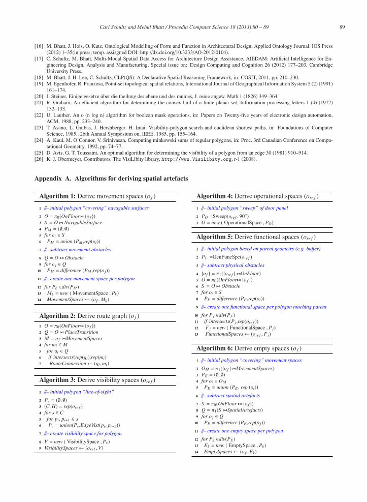
4.3. InSpace3D Modalities Component: Algorithms for Deriving Standard Spatial ArtefactsIn this section we provide detailed algorithms for generating the spatial artefact geometries as implemented in
the Modalities component of InSpace3D middleware, and we provide computational complexity results based on
the framework established in the Section 4.2 (the referenced algorithms are presented at the end of the paper).
Movement Spaces. Movement spaces are derived in Algorithm 1 from a building story reference object o f ,
and the route graph is derived in Algorithm 2. The binary relation OnFloor associates objects to the building
stories in which they are contained. The unary relation NavigableSurface lists the objects on which the agent can
maneuver, such as slabs. The unary relation Obstacle lists the objects that are barriers to movement such as walls
and pieces of furniture.
Visibility Spaces. Algorithm 3 derives the visibility space of a reference object. Deriving the visibility
space relies on the notion of edge-visibility which has not been as thoroughly investigated within computational
geometry as point-visibility, although current complexity results suggest that edge-visibility is significantly more
complex to calculate [25]. Thus we approximate the derivation of visibility spaces by taking unions of isovists
from the polygon vertices of the physical geometry.
Operational Spaces. Operational spaces are derived in Algorithm 4 from a door reference object ore f . The
derived geometries are (in this case) not based on the environment, and only take the reference object’s class
and physical geometry into account. Operational spaces are often derived by sweeping, extruding, translating,
rotating, and scaling parts of the physical geometry.
Functional Spaces. The specific geometry of a functional space can be completely customised by defining
the function GenFuncSpc; we assume that the buffer operation is applied by default. Once the initial functional
space geometry has been derived from the object’s physical geometry, the physical space of obstacle objects must
subtracted. We then remove any geometric regions that are topologically disconnected from the object’s physical
geometry. This is presented in Algorithm 5.
Empty Spaces. Empty spaces are derived in Algorithm 6 from a building story reference object o f . The
relation SpatialArtefacts lists those derived objects that are not considered empty space (depending on the specific
task). For example, SpatialArtefacts can be the union of FunctionalSpaces and OperationalSpaces.
4.4. Computational Complexity of Standard Spatial ArtefactsTable 1 presents the complexity analysis of the algorithms in Section 4.3; Ob is the number of obstacles, Oq
is the number of opaque objects, Op is the number of openings, Nv is the number of navagable surfaces, S is the
number of spatial artefacts used in defining empty spaces, Mv is the number of movement spaces. All counts are
assumed to only include objects on the parent object’s floor. The time complexity analysis is based on Section 4.2.
Determining the maximum artefacts per parent takes the domain restrictions described in Section 4.1 into account
for dividing regions. Thus, we are now able to investigate and compare the properties of artefacts independent
of the specific number of geometric primitives used in their representation. Operational and visibility spaces
have a one-to-one relationship with their parent objects. The number of empty spaces may grow more rapidly
than movement spaces depending on the distribution of shapes of the relevant artefacts. Adding and removing
obstacles influences all artefacts except operational spaces (assuming that the obstacles are also opaque), but can
only indirectly affect empty spaces.
87 Carl Schultz and Mehul Bhatt / Procedia Computer Science 18 ( 2013 ) 80 – 89
Table 1. Complexity analysis of spatial artefacts based on the
number of objects in the environment.
ArtefactMaximum perparent Time complexity Time notes
Movement Ob + 1 M = Nv + Ob, covering andO(MlogM) subtract obstacles