Instantaneous Harmonic Analysis and its Applications in Automatic Music Transcription Ali Jannatpour A Thesis in The Department of Computer Science and Software Engineering Presented in Partial Fulfillment of the Requirements for the Degree of Doctorate of Philosophy (Computer Science) at Concordia University Montr´ eal, Qu´ ebec, Canada July 2013 c ⃝ Ali Jannatpour, 2013
Transcript
Instantaneous Harmonic Analysis
and its Applications in
Automatic Music Transcription
Ali Jannatpour
A Thesis
in
The Department
of
Computer Science and Software Engineering
Presented in Partial Fulfillment of the Requirements
for the Degree of Doctorate of Philosophy (Computer Science) at
Concordia University
Montreal, Quebec, Canada
July 2013
c⃝ Ali Jannatpour, 2013
CONCORDIA UNIVERSITY
SCHOOL OF GRADUATE STUDIES
This is to certify that the thesis prepared By: Ali Jannatpour
Entitled: Instantaneous Harmonic Analysis and its Applications in Automatic Music Transcription
and submitted in partial fulfillment of the requirements for the degree of
DOCTOR OF PHILOSOPHY (Computer Science) complies with the regulations of the University and meets the accepted standards with respect to originality and quality. Signed by the final examining committee: Chair Dr. C. Chen External Examiner Dr. M. Pawlak External to Program Dr. Y.R. Shayan Examiner Dr. E. Doedel Examiner Dr. J. Rilling Thesis Co-Supervisor Dr. A. Krzyżak Thesis Co-Supervisor Dr. D. O’Shaughnessy Approved by
Dr. V. Haarslev, Graduate Program Director October 7, 2013 Dr. C. Trueman, Interim Dean Faculty of Engineering & Computer Science
Abstract
Instantaneous Harmonic Analysis and its Applications in Automatic Music
Transcription
Ali Jannatpour, Ph.D.
Concordia University, 2013
This thesis presents a novel short-time frequency analysis algorithm, namely Instan-
taneous Harmonic Analysis (IHA), using a decomposition scheme based on sinusoidals. An
estimate for instantaneous amplitude and phase elements of the constituent components of
real-valued signals with respect to a set of reference frequencies is provided. In the context
of musical audio analysis, the instantaneous amplitude is interpreted as presence of the
pitch in time. The thesis examines the potential of improving the automated music anal-
ysis process by utilizing the proposed algorithm. For that reason, it targets the following
two areas: Multiple Fundamental Frequency Estimation (MFFE), and note on-set/off-set
detection.
The IHA algorithm uses constant-Q filtering by employing Windowed Sinc Filters
(WSFs) and a novel phasor construct. An implementation of WSFs in the continuous
model is used. A new relation between the Constant-Q Transform (CQT) and WSFs is
presented. It is demonstrated that CQT can alternatively be implemented by applying a
series of logarithmically scaledWSFs while its window function is adjusted, accordingly. The
relation between the window functions is provided as well. A comparison of the proposed
IHA algorithm with WSFs and CQT demonstrates that the IHA phasor construct delivers
better estimates for instantaneous amplitude and phase lags of the signal components.
iii
The thesis also extends the IHA algorithm by employing a generalized kernel func-
tion, which in nature, yields a non-orthonormal basis. The kernel function represents the
timbral information and is used in the MFFE process. An effective algorithm is proposed to
overcome the non-orthonormality issue of the decomposition scheme. To examine the per-
formance improvement of the note on-set/off-set detection process, the proposed algorithm
is used in the context of Automatic Music Transcription (AMT). A prototype of an audio-
to-MIDI system is developed and applied on synthetic and real music signals. The results
of the experiments on real and synthetic music signals are reported. Additionally, a multi
-dimensional generalization of the IHA algorithm is presented. The IHA phasor construct
is extended into the hyper-complex space, in order to deliver the instantaneous amplitude
and multiple phase elements for each dimension.
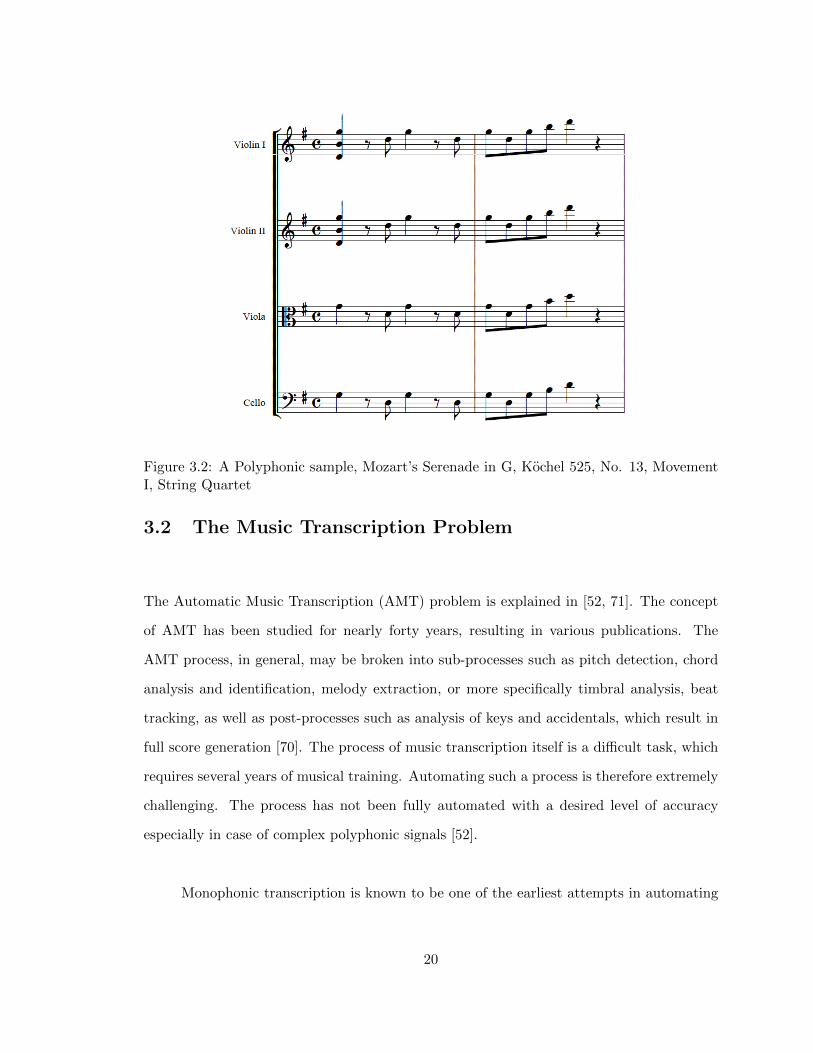
Index Terms: Instantaneous Harmonic Analysis (IHA), Short-Time Fourier Transform
3.1 Some Reported Results from the Literature . . . . . . . . . . . . . . . . . . 23
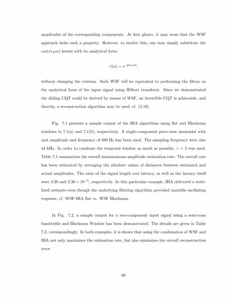
7.1 Overall estimation rate for instantaneous amplitude and full signal recon-struction of a sample signal using CQT, WSF and IHA. . . . . . . . . . . . 69
7.2 Overall estimation rate for instantaneous amplitude and full signal recon-struction of a two-component signal . . . . . . . . . . . . . . . . . . . . . . 69
M Discrete time window radiusQ Quality factorT Sampling periodγ Bandwidth resolution factorj The imaginary unitn Sample indext Time variableυ normalized frequencyω Angular frequency
Bk kth Bandfmin Minimum audible frequency
x(t) Real-valued continuous time domain signalx[n] Real-valued discrete time domain signal
Hk(t) The continuous IHA transformH[k, n] The discrete IHA transform
℘υ(x[n]) The IHA phasor construct
xvi
List of Abbreviations
ACF Auto-Correlation FunctionAMT Automatic Music TranscriptionANSI American National Standards Institute
MFFE Multiple Fundamental Frequency EstimationMIDI Musical Instrument Digital InterfaceMIR Music Information RetrievalMIREX Music Information Retrieval Evaluation eX-
SFFE Single Fundamental Frequency EstimationSTFT Short-Time Fourier TransformSVD Singular Value Decomposition
TEO Teager Energy Operator
WD Wigner DistributionWSF Windowed Sinc Filter
ZC Zero Crossing
xviii
Foreword
“In the name of Hermes, the god and the deity of the science of art1”
In the memory of Morteza Hannaneh (1923–1989), who believed music was not
only art but science.
Throughout the thesis, references to various musical terms are made. While the
reader is expected to be familiar with music terminology, a brief glossary is provided in
section 1.1. Throughout chapters 1–3 a brief introduction on the harmonic analysis and
music signal processing with a short survey on the state-of-the-art techniques is provided.
Chapters 4–7 provide the Instantaneous Harmonic Analysis (IHA) transform along with
its generalizations towards music signal processing, while chapter 8 solely focuses on music
transcription. It is hoped that the fundamental contribution of the IHA transform motivates
future research directions.
Ali Jannatpour,
October 2013, Montreal – Canada
1Quoted by Motreza Hannaneh during tutoring Practical Manual of Harmony by Nikolai Rimsky-Kor-sakov.
xix
Chapter 1
Introduction
Harmonic analysis may be understood as a special case of functional analysis in math-
ematics, which concerns studying functions and their representations based on superposition
of basic waves. The term harmonic originally comes from the eigenvalue problem, in which
the frequencies of the waves are integer multiples of the mother wave. Fourier analysis
may be considered in the context of Hilbert spaces, which provides a bridge between the
harmonic analysis and functional analysis. In music theory, however, harmonic analysis is
known as the study of chords and their combination in terms of producing musical effects.
This thesis concerns the former definition.
While harmonic analysis dates back to Fourier’s effort on analyzing the solutions of
the heat and wave equations, it has been widely used in many branches of science such as
mathematics, physics, and engineering, to name a few. Fourier series has been one of the
earliest attempts to study periodicity, by which an arbitrary periodic function is represented
1
by a sum of simple wave functions 1. The motivation of the Fourier transform comes from
generalization of the Fourier series when the period of the represented function is stretched
out and approaches infinity [48]. Such a definition delivers a sufficient measure for studying
the frequency distribution and provides a tool for studying non-periodic functions. The
periodicity itself has been studied in many branches of mathematics, which has resulted
in the topics such as definition of almost periodic functions, etc. The topic is an ongoing
research, especially in the generalization area [67].
Much effort has been devoted through the years to overcome the main drawback of the
classical Fourier transform, with respect to the loss of time information when the signal is
transferred into the frequency domain. Time-frequency analysis provides a compromise so-
lution by studying the signal simultaneously in the time and frequency domains. It has been
widely studied by many researchers in the literature. The Short-Time Fourier Transform
(STFT) has been one of the earliest approaches delivering a joint time-frequency analysis
[95]. It suggests applying the Discrete Fourier Transform (DFT) using a window function.
Assuming the input signal is quasi-stationary, STFT provides a two-dimensional time-fre-
quency analysis by taking the Fourier transform of the signal using a window function. Such
windowing results in a tradeoff in time resolution vs. frequency resolution. Wavelets, on the
other hand, provide frequency analysis at different resolutions by preserving the locality.
Wigner Distribution (WD) has been used by many researchers as a powerful time-
frequency analysis tool [65]. One of the advantages of WD over STFT is using a quadratic
function to avoid negativity in order to provide energy distribution. It however produces
undesirable cross-terms [89]. It has been demonstrated to have a fine performance, especially
1Convergence of the Fourier series has been studied extensively in the literature. In general, one canconsider point-wise, uniform, and L2 convergence. It is easy to show that a Fourier series of a periodicfunction f in L2 converges to f in L2 sense. Also a Fourier series of a periodic, integrable function which iscontinuous at x0 converges to f(x0). If f is periodic, continuous and differentiable on R with f ′ piecewisecontinuous then the Fourier series of f converges uniformly. Point-wise convergence is tricky. It was shownby Carleson [19] that Fourier series of any periodic function f ∈ L2 converges to f point-wise, almosteverywhere. Later on, Hunt [60] generalized the space to Lp for any p ∈ (1,∞). The main references on thetopic are [8, 113].
2
in the analysis of non-stationary signals [58].
Alternatively, the Instantaneous Frequency (IF) is defined based on analytical signals
where both amplitude and phase are represented by time-varying functions. IF is generally
calculated from the analytical signal using the Hilbert transform, although other variations
have been used in the literature, resulting in contradicting definitions [91]. The major
difference between IF and STFT is that STFT delivers a spectral analysis in a discrete
form, whereas IF provides an instantaneous measure at a frequency level. The STFT
allows studying multiple frequencies within a short time, while IF delivers the instantaneous
frequency of the signal in time. IF has been extensively used by many researchers. Although
there are numerous applications for IF-based signal analysis, some researchers challenge the
concept stating that it violates the uncertainty principle (see [51]).
The uncertainty principle states that the signal cannot simultaneously be localized in
both time and frequency. It may alternatively be understood as the Gabor limit, stating that
a function cannot be both time-limited and band-limited at the same time [43, 88]. Several
papers have been published on the topic of the relation between the time-resolution and
the bandwidth, mainly suggesting an upper limit for the product of the two. This relation
plays a great role in short-time frequency analysis, especially when estimating instantaneous
properties are targeted. A mathematical survey on the topic may be found in [41].
The concept of IF has provoked strong opinions among scientists with respect to
the uncertainty principle [59]. Cohen has published a significant paper [28] on the topic
of the product of time and frequency covariances. He states that the reason behind so
much confusion on the uncertainty principle is mainly due to misinterpretation of STFT
philosophy.
In frame-based analysis [6] where the signal is segmented into smaller pieces, it is
3
assumed that the signal is completely stationary within the frame. In case the stationary
property cannot be satisfied, smaller frames may be used. However, the frames cannot be
made arbitrarily small, for many different reasons, the most importantly, the uncertainty
principle. Hence, a need for non-stationary signal analysis is beneficial.
One practical domain of non-stationary signal processing is the analysis of music
signals. Music signals have a certain specific characteristics. For instance, they follow
the pattern of musical scales which represent a discrete set of frequencies; the discrete
frequencies are logarithmically spaced on the frequency axis; and, the presence of notes in
time forms the melody. In this thesis, we focus on short-time frequency analysis approaches,
specific to the non-stationary time-frequency characteristics of the music signals.
Several attempts have been made for choosing the best joint time-frequency resolu-
tions based on the application [94]. For instance, in the context of tonal music analysis,
considering the way that the musical scales are structured, applying a logarithmic spectral
analysis is more effective than using a linear paradigm [49]. In an equal temperament sys-
tem [7], the frequency ratio of the two notes within an equal interval is always constant.
Therefore, the frequencies follow a logarithmic scales. Constant-Q Transform (CQT) is one
of the approaches that provides a logarithmic spectral analysis with respect to the equal
temperament that is used in western music [16]. It is based on the theory behind DFT, but
uses a constant ratio of center frequency to resolution that is equivalent to one semitone.
CQT can generally be performed by taking the Fourier transform of a windowed sequence
where the window is a function of the product of time and frequency. Prior to introducing
CQT by Brown, constant-Q analysis has been used in the literature. For instance, Kates [66]
previously showed that the result of a constant-Q analysis using an exponentially decaying
window is equivalent to the Z-transform along an outwardly going spiral in the complex Z
4
-plane 2.
General issues about instantaneous amplitude and phase of signals have been dis-
cussed in [91]. This thesis proposes a new model for estimating instantaneous amplitude
and phase of multi-component signals which may be used as a fundamental tool in Multi-
ple Fundamental Frequency Estimation (MFFE). MFFE, or multiple-F0 estimation, is an
essential process in audio analysis by addressing the over-toning issue, which is caused by
harmonic collisions from two or more simultaneous tones. A tone is a steady periodic sound,
often generated by a musical instrument, that plays a musical note. It is not necessarily
a pure tone. A non-pure tone may be decomposed into one pure fundamental tone and a
some overtones [70].
In Single Fundamental Frequency Estimation (SFFE), a signal is assumed to consist
of single Fundamental Frequency (F0) at a time. Therefore, estimating F0’s is a straightfor-
ward process. In MFFE, however, the harmonic collision of the multiple overtones makes
the process rather difficult. The harmonic collision is caused by the interferences of the
overtones produced by multiple sources (i.e. an octave or a perfect fifth). This is very
common in music where the multiple sources form consonant intervals [7].
1.1 Terminology
The thesis discusses the harmonic analysis of multi-component tonal audio signals. While
the formal specification of the analysis id provided in chapters 4–6, the used terminology is
2Z-transform converts a discrete time-signal into a complex frequency-domain representation:
Zx[n] =
+∞n=−∞
x[n]z−n
5
given in the following:
Multi-Component Signal: is an audio signal composed of musical tones.
Tonal Signal: is referred to an audio signal that consists of perfectly pitched
tones, corresponding to the standard musical notes. Musical notes correspond to
a discrete set of frequencies, each of which, designate the fundamental frequency
of the note (i.e. 440 Hz for the standard concert pitch).
Transcription System: in simple words, is a system of converting an audio
signal into a set of note events that can be represented in a musical notation
format.
Throughout the thesis, various references to music terms are made. They are briefly ex-
plained in the following, while a comprehensive guide may be found in [46].
Accidentals: are note modifiers, which cause a pitch change that does not be-
long to the scale.
Cent: is a logarithmic micro-tonal unit of measure used for musical intervals,
equivalent of one-hundredth of a semitone.
Chord: is a harmonic set of three or more notes that is played simultaneously.
Diatonic Scale: is an eight-note scale composed of seven notes and a repeated
octave.
Harmony: is the use of simultaneous notes, usually in form of a chord. It often
refers to the vertical sonority of the music.
Harmonic: is an overtone whose frequency is an integer multiple of the funda-
mental frequency.
Interval: is the difference between two pitches, usually on a diatonic scale.
6
Melody: is a rhythmic sequence of single notes. It is often regarded as hori-
zontal, since the notes are played from left-to-right.
MIDI: Musical Instrument Digital Interface, is an industry specification for
encoding, storing, synchronizing, and transmitting the musical performance,
primarily based on note events.
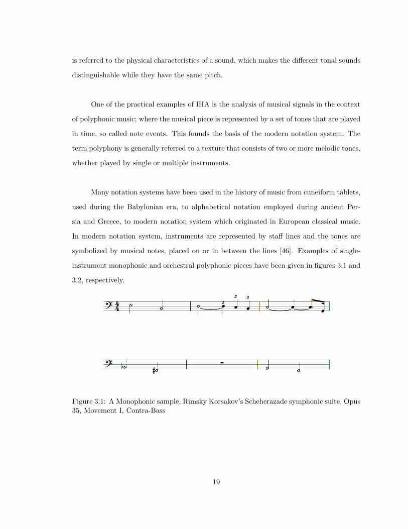
Notation: is a system used in sheet music in order to represent a piece of mu-
sic.
Note: identifies a pitched sound and is associated with a name (and sign).
Notes may be considered as atoms of music that allows discretization of musical
analysis.
Note Events: are the set of events identifying notes on-sets and off-sets.
Octave: is an interval between a note and its second harmonic.
Overtone: is a component of a sound with a frequency higher than the funda-
mental frequency.
Pitch: may be defined as the degree of highness or lowness of a tone on a fre-
quency-related scale.
Rhythm: is the timing of musical sounds and silences.
Semitone: is the smallest interval used in Western music and is equivalent to
one-twelfth of an octave. It is sometimes known as half-tone or half-step.
Scale: is a set of musical notes ordered by pitch.
Staff: is a set of five horizontal lines and four spaces that each represent a
different note.
Timbre: also known as tone color or tone quality, is referred to the physical
characteristics of a sound, which makes the different tonal sounds distinguish-
able while they have the same pitch.
Tone: is a steady periodic sound, often generated by a musical instrument, that
plays a musical note3.
3In some context, tone may also refer to the musical interval, equivalent to a major second. To distinguishbetween the two, we refer to the latter as whole-tone.
7
1.2 The Scope of the Thesis
This thesis primarily concerns the problems and challenges of the Instantaneous Harmonic
Analysis (IHA) of audio signals, with a focus on non-stationary signal analysis techniques.
The challenges include multi-pitch analysis, MFFE, harmonic collision, overtone estimation,
to name a few. The thesis targets the two core areas in music transcription: MFFE and note
events detection. The audio analysis in this thesis is purely tonal and therefore percussion
analysis is out of the scope of this thesis.
A novel harmonic analysis algorithm, namely IHA, is provided based on enhanced
Constant-Q filtering. The IHA algorithm delivers a signal decomposition scheme based
on the frequency distribution of musical scales. The objective of the IHA algorithm is to
provide the instantaneous amplitudes and phase lags of the signal components with respect
to the discrete set of frequencies that are associated with the musical scales. It can be used
as a fundamental tool for MFFE where the instantaneous amplitudes represent the presence
of fundamental frequencies in time, and the instantaneous phase lags are used for overtone
estimation.
The scope of the thesis is to implement and evaluate the performance of the new
algorithm in the context of musical signal analysis. The performance is measured by evalu-
ating the improvement of the note events detection process, by applying the algorithm on
different sets of musical data in order to produce the note events. Note events, in simple
words, are referred to as the representation of music pieces in form of note on-sets and off-
sets. They are the essential part of the music and form the core of the music notation [46].
8
The thesis contributes to the music analysis, yet it does not aim at automating the whole
music transcription process.
1.3 Thesis Contributions
The thesis delivers a novel IHA algorithm based on enhanced Constant-Q filtering [62]. An
implementation of Windowed Sinc Filters (WSFs) based on the signal model in its original
continuous form has been used. A new relation between the CQT and WSFs has also been
provided [63]. The thesis also extends the IHA transform by employing a generalized kernel
function. The algorithm contributes to an MFFE process where a post-processing overtone
elimination algorithm is used for timbral analysis. A generalization in multi-dimensional
space has also been provided.
1.4 Thesis Organization
The thesis is structured as follows: A background on harmonic analysis algorithms and
related transformations and the motivation of the thesis is given in the next chapter. A
short survey of related music signal processing techniques is provided in chapter 3. The
formal specification of the IHA transform is given in chapter 4. Chapter 5 presents the
generalization of the IHA transform into the multi-dimensional space. The generalization of
the IHA algorithm for timbral analysis is formalized in chapter 6. The theoretical analysis
of the IHA algorithm along with the relation between WSFs and CQT is presented in
chapter 7. The transcription system as well as the post-processing algorithms are discussed
in chapter 8. And in chapter 9 the thesis is concluded.
9
Chapter 2
Background and Motivation
This chapter discusses the background and motivation behind this thesis. A short
survey of time-frequency analysis algorithms with an emphasis on CQT is presented.
The signal decomposition scheme that is used in the thesis is discussed here.
The STFT has been one of the earliest attempts delivering a joint time-frequency
analysis [95]. Huang et al. [59] provided a comprehensive survey on instantaneous frequency
-based methods in particular Zero Crossing (ZC), Teager Energy Operator (TEO), and
normalized Hilbert transform, to name a few. A historical review on instantaneous frequency
was previously provided in [14, 15]. Rabiner and Schafer utilized the STFT in [95], which
was also surveyed by Kadambe and Boudreaux-Bartels [65] along with the WD and wavelet
theory. Khan et al. [68] proposed an IF estimation using fractional Fourier transform and
WD.
IF has been widely used by many researchers in the literature. It is generally calcu-
lated from the analytical signal using the Hilbert transform [91]. Oliveira and Barroso used
10
the IF of multi-component signals in [87]. Nho and Loughlin studied IF and the average
frequency crossing in [86]. An Empirical Mode Decomposition (EMD) based-method is also
used by Zhang et al. in [111] for IF estimation. Arroabarren et al. in [5] have provided some
methodological basis for determining the instantaneous amplitudes and frequencies.
In the context of tonal music analysis, considering the way that the musical scales
are structured, applying a logarithmic spectral analysis is more effective than using a linear
paradigm. CQT, originally introduced by Brown, is one of the approaches that provide
such spectral analysis [16]. Brown explained how such analysis can be improved by using
a spectral representation that supports the logarithmic spacing of the musical tones. She
states that one of the major advantages of such representation is that the spectral com-
ponents form a pattern in the frequency domain which is the same for all sounds with
harmonic frequency components [16]. Therefore, using a constant ratio of center frequency
to resolution, namely Q, is highly efficient in comparison with using a constant bandwidth
resolution that is used in the traditional DFT-based approaches. Brown explained that one
of the major advantages of such design is that the spectral components form a pattern in
the frequency domain that is the same for all sounds with harmonic frequency components.
In the following sections, the formal definition of CQT is given. CQT is used in this
thesis, in relation with the signal decomposition scheme. The signal decomposition scheme is
subsequently discussed. The frequency quantization delivered by the decomposition scheme
is explained. This chapter concludes with the motivation behind the thesis.
11
2.1 The Constant-Q Transform
CQT is calculated by taking the Fourier transform of a windowed sequence while the window
is a function of the product of time and frequency. The constant ratio represents the quality
factor and is set to the number of full cycles to be used by the temporal window. The formal
definition of CQT is as follows [16].
Given x[n], the input signal in discrete domain, the CQT of x[n] is defined as:
X[k] =1
N [k]
N [k]−1n=0
W [k, n] ·x[n] · e−j2πQn
N [k] (2.1)
where N [k] represents the temporal window length,
N [k] =Q
Tfk,
and Q and fk are the quality factor and the kth reference frequency, respectively. W [k, n]
denotes a symmetric window function, e.g., Hamming window. The above equation may
also be understood as taking a normalized Fourier transform of the windowed signal by
using a predefined set of digital frequencies and applying a temporal window with the exact
Q number of cycles. It must be noted that x[n] in (2.1) represents the windowed signal. cf.
[16].
The invertibility of CQT has been a challenge for years. Although filter bank ap-
proaches are invertible in nature, the inverse transform for the CQT algorithm had not
been available until recently. The first attempt of obtaining the inverse transform was
made by Cranitch et al. [30]. The authors explained that the process could not formally be
inverted as the matrix representation of the CQT implementation by DFT uses non-square
matrices. They provided the solution using a pseudo-inverse of the transform matrix, by
taking advantage of the scarcity property of the DFT, due to the fact that the time domain
12
signal is properly pitched. Holighaus et al. [56] recently provided a framework for calcu-
lating an invertible CQT in real-time. Their work was based on the non-stationary Gabor
frames [6, 20]. Ingle and Sethares [61] also developed a least-square invertible constant-Q
spectrogram for phase vocoding.
2.2 The Decomposition Scheme
Signal decomposition is a broad topic that addresses the functional relationship between an
arbitrary signal and its constituent components by which the original signal can be recon-
structed. Depending on the application, different decomposition paradigms may be used.
While frame theory provides an orthonormal basis for signal decomposition, alternative
schemes may also be used based on the application.
In tonal music analysis, where the input signal is perfectly pitched, it is desired to
study signals at certain frequencies. These frequencies correspond to musical notes and the
analysis examines the existence of such frequencies in short time. Hence, one may look for
a decomposition scheme to transform input signals into a set of pure components that can
be later on used within an MFFE process. In such a model, the reference pitches form
the musical scale and are chosen according to the intonation system [7] (cf. [16], harmonic
sounds in [71]). Since each tone is represented by a fundamental frequency, estimating the
presence of such frequencies is the key to the note identification process [26].
In our model, a multi-component signal may be decomposed into a finite number
of single-component signals, each of which represents a pure tone in the form of a quasi-
sinusoidal:
x(t) =k
Ck(t), (2.2)
13
where
Ck(t) = ak(t) cos(ωkt+Φk(t)), (2.3)
represents the kth component, ak(t) and Φk(t) represent the instantaneous amplitude and
phase lag of the kth component, respectively. ωk’s represent the frequencies and are loga-
rithmically spaced on the frequency axis:
ωk+1 = γ ·ωk, γ > 1, ωk > 0. (2.4)
2.3 Frequency Quantization
Eq. (2.4) conveys a logarithmic quantization of the frequency axis. The frequency axis is
quantized into a set of small intervals by maintaining the constant-Q whereas the reference
frequencies are logarithmically centered on the corresponding intervals. Brown’s quality
factor Q was originally defined in the discrete domain based on the window size in the time
resolution. One may redefine such a measure by using the frequency resolution instead (cf.
[28]). In such definition, the time domain need not be necessarily discretized. This allows
us to apply the filters in both discrete and continuous forms. Our approach is based upon
a map function Ω : Z→ R× R2, as follows.
Given ω0, the global reference frequency, and γ > 1, the bandwidth resolution factor,
the map function Ω quantizes the frequency axis into a set of bands Bk, each of which is
tagged with a reference frequency ωk, where the reference frequency is centered in the band.
In this model, the bandwidths are proportional to the frequencies. The definition of the
map function is given in the following:
Ω(k) = ⟨ωk, Bk⟩ , (2.5)
14
where
ωk = γkω0,
|Bk| = λωk,
and |Bk| denotes the bandwidth and λ is a function of γ.
A full partition of the frequency axis may be achieved by choosing non-overlapping Bk’s,
as in the following:
Bk ∩Bl = ∅, k = l withk Bk = [0,Ω] ,
where Ω denotes the bandwidth of the signal. However, in general, Bk may be chosen as
(1− λ
2)ωk, (1 +
λ
2)ωk
, (2.6)
or ωk
1√γ, ωk√γ
, (2.7)
whether ωk is linearly or logarithmicaly centered in Bk, respectively. It must be noted that
in case (2.6) is used, λ < 2 must hold. Also, for small bandwidths, λ→ γ.
In practice, the map function Ω is bounded. Although ω0 is chosen arbitrarily, it is
commonly set to 880π, representing A440, the standard concert pitch, or to a minimum
frequency, i.e. the minimum audible tone or the lowest frequency of the musical instruments
/ vocals in use. The bandwidth resolution may also be represented in cents,
c = 1200 log2 λ
an equivalent of one-hundredth of a semitone [7]. A 50-cent or a 100-cent resolution may
be used whether a 12 or 24 equal temperament system is desired [32]. The two systems
15
are used in western and quarter-tone music, respectively [38]. The equivalent bandwidth
resolution factors of such resolutions are 1.0293 and 1.0595, or in Brown’s system 69.25 or
34.62, respectively. The relationship between Brown’s quality factor and our bandwidth
resolution factor may also be obtained by (cf. [28, 16]):
1
Q=λ− 1
2. (2.8)
2.4 Motivation of the IHA Algorithm
The objective of our model is to find a set of pairs of time-varying functions ak(t), Φk(t) in
(2.3), that best estimate the instantaneous amplitude and phase lag of the signal compo-
nents. Our approach is based upon two constraints:
1. ωk’s are known, and
2. ak’s and Φk’s are smooth functions such that they can be locally approximated by a
constant 1.
ωk’s form the standard musical tones, and the constraints on ak’s and Φk’s makes it possible
to use a linear approach, i.e., the first derivative, for the estimation2. The details are given
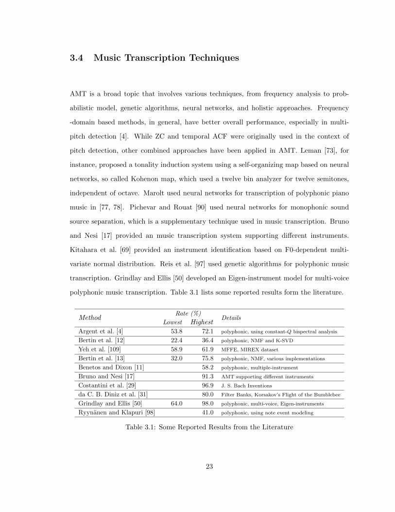
[4]. Purwins et al. [93] used CQT for modulation tracking. CQT has also been used in
source separation [96]. Different variations of Constant-Q approach have been used in the
literature. For example, Graziosi et al. earlier proposed a modified version of the Constant-
24
Q, so called mCQFFB, by improving the response characteristics of Fast Filter Bank (FFB)
[34, 49]. da C. B. Diniz et al. [31] provided a practical design of filter banks in the AMT
context. Argent et al. [4] proposed using CQT for both pitch and onset estimation. A
comprehensive survey may be found in [57].
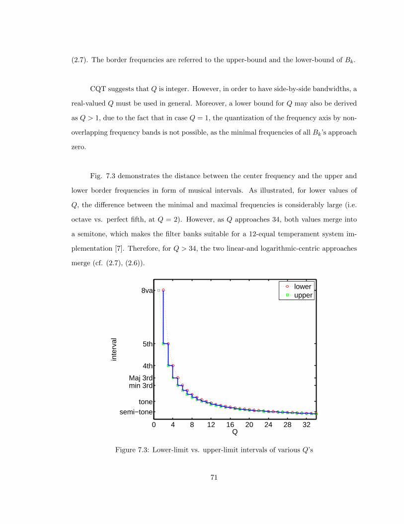
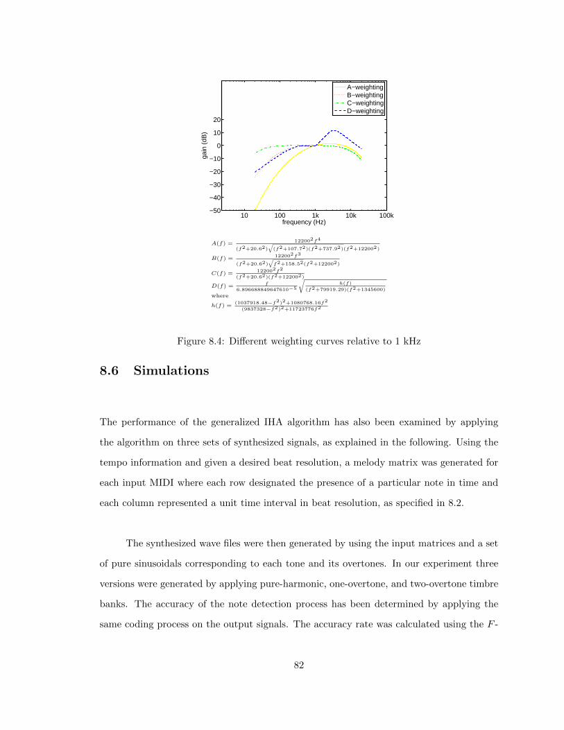
3.6 Summary
An overview of music signal analysis with the focus on music transcription was provided.
A survey of related work was given with an emphasis on CQT in polyphonic transcription,
and the importance of MFFE and note events analysis in music transcription. In the next
chapter, we develop our harmonic analysis algorithm, which in nature is a time-frequency
transformation targeted for music analysis. The algorithm is used in this thesis for MFFE
and the note events detection.
25
Chapter 4
The IHA Transform
This chapter presents our novel short-time frequency analysis algorithm. Given a set
of reference pitches, the objective of the algorithm is to transform the real-valued time-
domain signal into a set of complex time-domain signals in such a way that the amplitude
and phase of the resulting signals represent the amplitude and phase of the signal
components with respect to a set of reference pitches. The specification of the IHA
algorithm as well as the phasor construct for both continuous and discrete forms is
provided, in here. The chapter also contributes to the fast real-time implementation of
an M + 1-delay IHA algorithm.
The IHA problem may be defined as the following. Given an input signal, the objective
of the approach is to find a set of pairs of time-varying functions, representing instantaneous
amplitude and phase of the signal components. The problem may be broken into two main
sub-problems: signal decomposition, and instantaneous amplitude phase estimation. As
there are numerous approaches for decomposing an arbitrary signal into its components,
our proposed approach is based on constant-Q analysis which is well suited for the processing
musical signals.
26
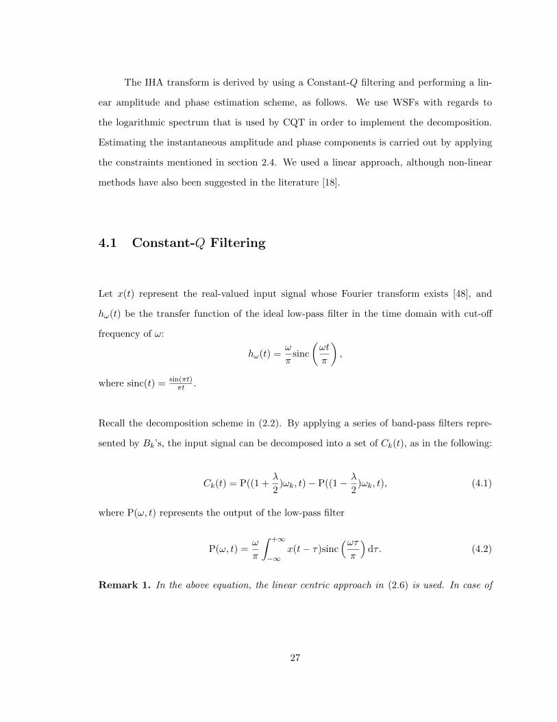
The IHA transform is derived by using a Constant-Q filtering and performing a lin-
ear amplitude and phase estimation scheme, as follows. We use WSFs with regards to
the logarithmic spectrum that is used by CQT in order to implement the decomposition.
Estimating the instantaneous amplitude and phase components is carried out by applying
the constraints mentioned in section 2.4. We used a linear approach, although non-linear
methods have also been suggested in the literature [18].
4.1 Constant-Q Filtering
Let x(t) represent the real-valued input signal whose Fourier transform exists [48], and
hω(t) be the transfer function of the ideal low-pass filter in the time domain with cut-off
frequency of ω:
hω(t) =ω
πsinc
ωt
π
,
where sinc(t) = sin(πt)πt .
Recall the decomposition scheme in (2.2). By applying a series of band-pass filters repre-
sented by Bk’s, the input signal can be decomposed into a set of Ck(t), as in the following:
Ck(t) = P((1 +λ
2)ωk, t)− P((1− λ
2)ωk, t), (4.1)
where P(ω, t) represents the output of the low-pass filter
P(ω, t) =ω
π
+∞
−∞x(t− τ)sinc
ωτπ
dτ . (4.2)
Remark 1. In the above equation, the linear centric approach in (2.6) is used. In case of
27
using (2.7), the output components will be:
Ck(t) = P(ωk√γ, t)− P(ωk
1√γ, t).
Recall the decomposition scheme in section 2.2. In our model, the input signal is
composed of quasi-sinusoidals whose frequencies are ωk’s. The quasi-sinusoidal, in here,
may be understood as a wave form that best fits a piecewise sinusoid. Various models of
quasi-sinusoidals have been used in the literature. For instance, in using K-partials [35], a
blind estimation approach can be used for estimating sinusoidal parameters. Partials refer
to the fundamental frequency and the overtones. Shahnaz et al. [101] used a different model
of K-partials, similar to our approach, for single pitch estimation. We will show later on
how their model fits in our model.
Eq. (4.1) specifies the implementation of our constant-Q filtering. Graziosi et al. used
a discrete constant-Q filter bank in [49]. Our approach applies the filter bank in the con-
tinuous form. Using the continuous implementation has many advantages. For instance, it
provides utilizing theoretical approaches by using a continuous model of the signal. We will
show how our implementation can improve the estimation of the instantaneous amplitude
and phase functions.
4.2 Amplitude and Phase Estimation
Recall (2.2). Assuming Bk’s are sufficiently small and Ck(t) approximately represents the
kth quasi-sinusoidal component, we can write:
Ck(t) ≈ ak(t) cos(ωkt+Φk(t)).
28
By taking derivative of both sides of the equation, we obtain:
d
dtCk(t) ≈
d
dtak(t)
· cos(ωkt+Φk(t))− ak(t) ·
ωk +
d
dtΦk(t)
· sin(ωkt+Φk(t))
Since ak(t) and Φk(t) are locally constant, for small ∆t, we write:
Ck(t−∆t) ≈ ak(t) cos(ωk(t−∆t) + Φk(t))
Ck(t+∆t) ≈ ak(t) cos(ωk(t+∆t) + Φk(t))
.
As ∆t→ 0
ddtak(t) ≈ 0, d
dtΦk(t) ≈ 0.
therefore:
Ck(t)−j
ωk
d
dtCk(t) ≈ ak(t)ej(ωkt+Φk(t)).
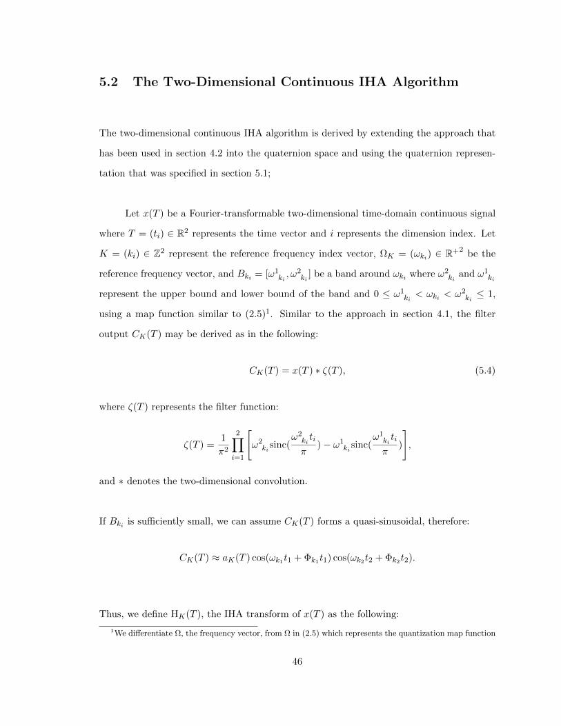
Thus, we define Hk(t), the continuous IHA transform of x(t) as
Definition 1 (The continuous IHA transform). The continuous IHA transform of x(t) with
respect to the map function Ω is defined as:
Hk(t)def= e−jωkt
1− j
ωk
d
dt
Ck(t). (4.3)
where Ω(k) = ⟨ωk, Bk⟩ as specified in (2.5).
x(t) may then be fully reconstructed using:
x(t) = ℜ
k
Hk(t)ejωkt
The magnitude of the time-varying complex function Hk(t) in (4.3) delivers the estimates
for instantaneous amplitude of the component Ck. It also presents the existence of reference
29
frequency ωk in time.
4.3 Discretization
In practical applications, real signals are generally sampled and represented in the discrete
form. Therefore, the Constant-Q filtering as well as the amplitude and phase estimation
algorithms must be provided in the discrete form, as well. Various approaches have been
proposed in the literature for implementing band-pass filtering in the discrete form, most
of which are based on DFT. CQT uses STFT for applying short time windows in order
to calculate the DFT. It provides acceptable results, especially in combination with other
approaches (cf. [4, 49, 31]). We propose using a different approach by remodeling the
signal in its original continuous form. This significantly improves the estimation of the
instantaneous amplitude and phase functions in the discrete form1.
In our approach,
1. the discrete signal is initially interpolated in order to be remodeled in the continuous
form;
2. the continuous signal is then filtered and the filter outputs are generated;
3. and the result is subsequently represented in the discrete form.
For simplicity, we use the Nyquist-Shannon algorithm among other interpolation techniques.
The details are given in the following.
1The performance analysis is provided in chapter 7.
30
Let x[n] represent our discrete signal. If the input signal is a perfectly pitched audio,
it can be assumed that the signal consists of a set of piece-wise quasi-sinusoidal components.
Therefore, given x[n], a sequence of numbers in the real domain, representing a sampled
signal with the sampling period T , where n is an integer and denotes the sample index, the
signal decomposition will become:
x[k] =k
C[k, n],
where
C[k, n] = a[k, n] cos(nωkT +Φ[k, n]).
C[k, n]’s in the above equation represent the harmonic sinusoidals.
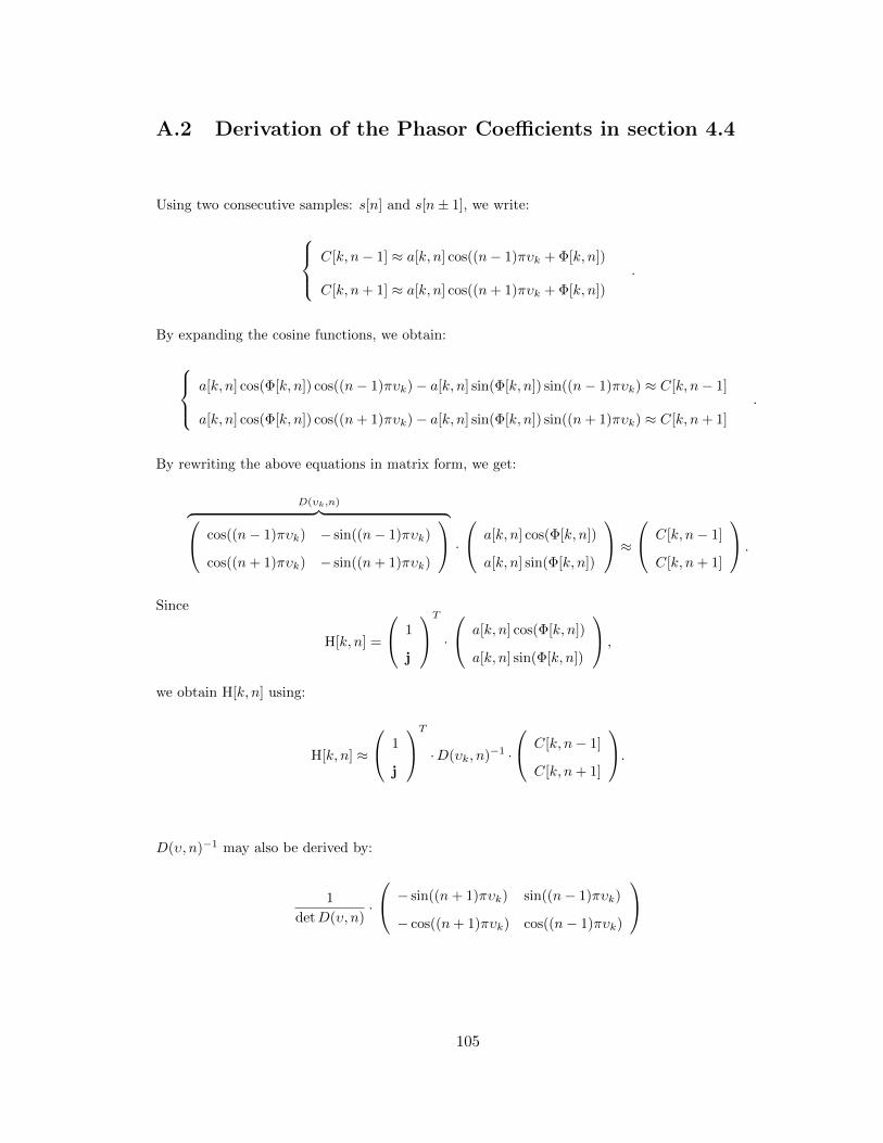
4.4 Derivation of the IHA Transform
Suppose x is band-limited and contains no frequencies higher than π/T where T represents
the sampling period. Using sampling theorem2, x can be reconstructed using the following
[76]:
x(t) =
+∞m=−∞
x[m]sinc
t−mTT
. (4.4)
It can be shown that x[m] = x(mT ).
To derive the IHA transform, we apply the band-pass filters represented by Bk’s on the
signal model in the continuous form. Using (4.2), the output of the ideal band bass filter
2The Shannon interpolation formula is used for simplicity, as the convolution of the sinc kernel and thelow-pass filter function is indeed a sinc function. However, one may use a more modern sampling approach.Comprehensive overview of modern sampling theory may be found in [55, 36, 107]. The infinite latencyproperty of the sinc filters is addressed in section 4.5.1.
31
will become:
P(ω, t) =
+∞m=−∞
x[m]ωT
πsinc
ωt−mωT
π
,
where 0 ≤ ω ≤ π/T .
By rewriting the above equation in the discrete form (t = nT ), we will have:
P(ω)[n] =
+∞m=−∞
x[m]ωT
πsinc
ωT
π(m− n)
.
P may also be rewritten as:
P(υ)[n] =+∞
m=−∞υsinc (υ(m− n))x[m], (4.5)
where
υ = ωTπ , 0 ≤ υ ≤ 1, (4.6)
is to be called the normalized frequency, as (4.5) is independent of T . The normalized
frequency is expressed in number of half-cycles per sample. Some authors have used the
product of the frequency and the sampling period as the normalized frequency (cf. [4]).
Definition 2 (The normalized frequency). The normalized frequency υ with respect to the
sampling period T is defined as (4.6).
By using (4.2) and (4.5), we may obtain the filter response C[k, n] as in the following3. For
simplicity, m is shifted by n.
C[k, n] =
+∞m=−∞
x[m+ n]Fk[m],
3cf. Appendix A.1
32
where
Fk[m] = υk · (1 +λ
2) · sinc
υk(1 +
λ
2)m
− υk · (1−
λ
2) · sinc
υk(1−
λ
2)m
,
represents the discrete constant-Q filter, m ∈ Z, and υk represents the kth normalized
frequency with respect to T . Fk[m] may also be simplified as:
Fk[m] = λ · υk · sincλmυk2
cos(πυkm). (4.7)
Remark 2. In case of using logarithmic centric approach as in (2.7):
Fk[m] = υk√γsinc (mυk
√γ)− υk
1√γsinc
mυk
1√γ
.
The final step to formulate the discrete IHA transform is to implement the estimation
algorithm in the discrete form. In order to best fit C[k, n] into a piece-wise sinusoid, we
assume that a[k, n] and Φ[k, n] are locally constant. Hence, we can write:
C[k, n] ≈ a[k, n] cos(nπυk +Φ[k, n]).
By using the similar approach as in section 4.2, we can estimate the instantaneous amplitude
and phase components by using two consecutive samples, and maximizing the likelihood of
having equal amplitudes and a πυk phase lag:
C[k, n− 1] ≈ a[k, n] cos((n− 1)πυk +Φ[k, n])
C[k, n+ 1] ≈ a[k, n] cos((n+ 1)πυk +Φ[k, n])
.
By representing a[k, n] and Φ[k, n] in their phasor representation,
H[k, n] = a[k, n]ejΦ[k,n],
33
we can estimate the phasor coefficients using4:
H[k, n] ≈
1
j
T
·D(υk, n)−1 ·
C[k, n− 1]
C[k, n+ 1]
,where
D(υ, n) =
cos(nπυ − πυ) − sin(nπυ − πυ)
cos(nπυ + πυ) − sin(nπυ + πυ)
.By resolving D(υ, n)−1 we can simplify the result. Therefore, using the map function Ω,
we derive the discrete IHA transform of x[n], a sequence in the complex domain, as given
in the following. The definition of the map function Ω is given in (2.5).
Definition 3 (The discrete IHA transform). The discrete IHA transform of x[n] with respect
to the map function Ω is defined as:
H[k, n]def= e−jπυkn ·℘υk (C[k, n]) , (4.8)
where ℘ is the IHA phasor construct, as defined below:
℘υ(x[n])def=
j
sin 2πυ
e−jπυ
−ejπυ
T
·
x[n− 1]
x[n+ 1]
.
The above construction transforms the real-valued component into its instantaneous phasor
representation.
4cf. Appendix A.2
34
4.5 Implementation
This section presents the implementation of constant-Q filtering based on WSFs and the
signal model in its original continuous form, which was presented in section 4.3.
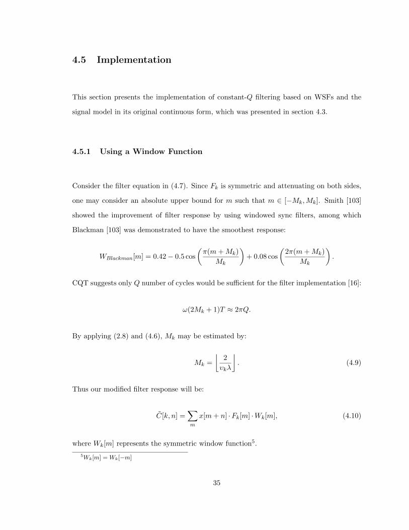
4.5.1 Using a Window Function
Consider the filter equation in (4.7). Since Fk is symmetric and attenuating on both sides,
one may consider an absolute upper bound for m such that m ∈ [−Mk,Mk]. Smith [103]
showed the improvement of filter response by using windowed sync filters, among which
Blackman [103] was demonstrated to have the smoothest response:
WBlackman[m] = 0.42− 0.5 cos
π(m+Mk)
Mk
+ 0.08 cos
2π(m+Mk)
Mk
.
CQT suggests only Q number of cycles would be sufficient for the filter implementation [16]:
ω(2Mk + 1)T ≈ 2πQ.
By applying (2.8) and (4.6), Mk may be estimated by:
Mk =
2
υkλ
. (4.9)
Thus our modified filter response will be:
C[k, n] =m
x[m+ n] ·Fk[m] ·Wk[m], (4.10)
where Wk[m] represents the symmetric window function5.
5Wk[m] =Wk[−m]
35
4.5.2 Frequency Upper Bound
One of the key constraints in using sampling theorem is that the signal is to be band-limited.
As a result, the center frequencies υk’s are bounded, as well. For instance, in case of using
(2.6), the upper bound for υk may be obtained by6:
υk ≤2
λ+ 2
Remark 3. In case of using logarithmic centric approach, the following inequality may be
used:
υk ≤1√γ
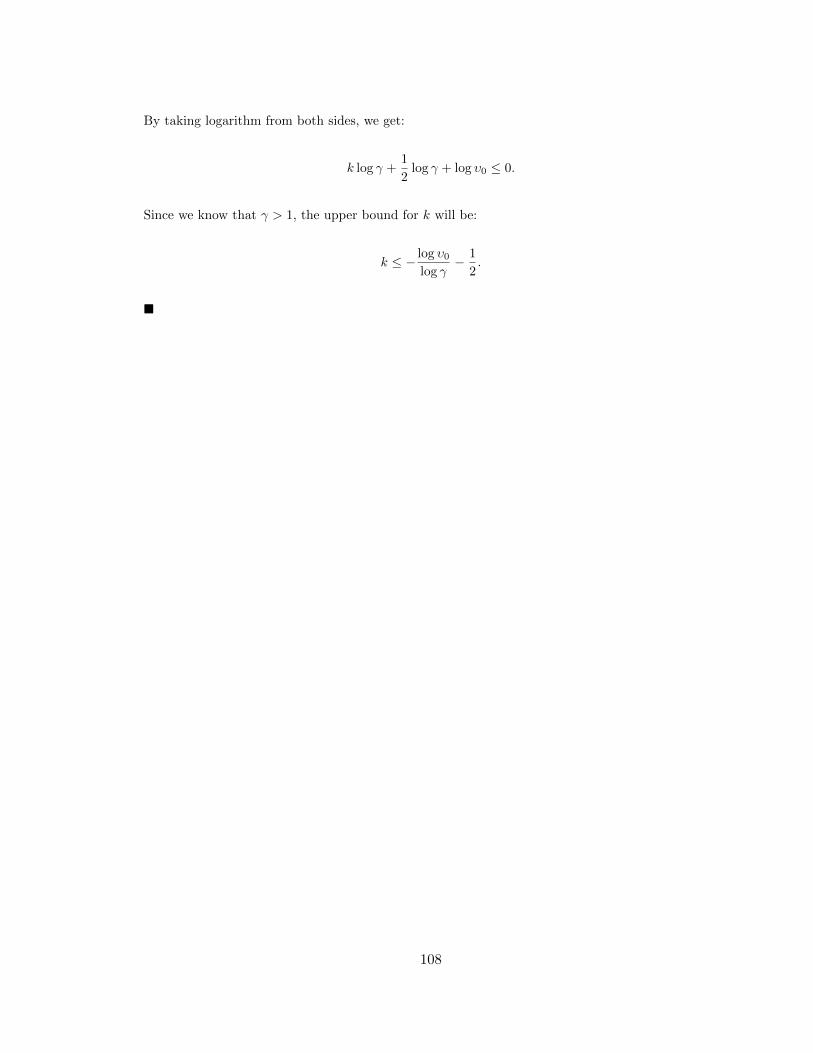
Therefore, given υ0, the normalized global reference frequency were 0 < υ0 < 1, the upper
bounds for k, the frequency index, may be obtain by using (2.5), as in the following:
k ≤ − 1
log γ(log υ0 + log(λ+ 2)− log 2)
Remark 4. Similarly, in case of using logarithmic centric approach, upper bound for k will
be:
k ≤ − log υ0log γ
− 1
2
4.5.3 Frequency Lower Bound
Eq. (4.9) also indicates that the number of samples that are required for each iteration
increases as υk approaches lower frequencies. In practice, where there exists a time quantum,
one may consider an upper bound forM . Hence, the lower bound for the reference frequency
6cf. Appendix A.3
36
can be derived using γυk as the frequency resolution (cf. [28]):
υk ≥2
Mmaxλ.
A lower bound for k may also be obtained by:
k ≥ 1
log λ(log 2− logMmax − log υ0)− 1.
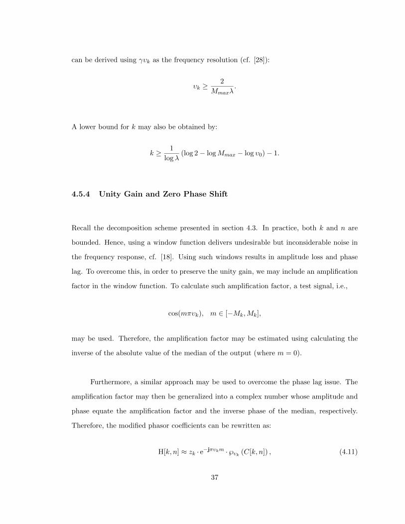
4.5.4 Unity Gain and Zero Phase Shift
Recall the decomposition scheme presented in section 4.3. In practice, both k and n are
bounded. Hence, using a window function delivers undesirable but inconsiderable noise in
the frequency response, cf. [18]. Using such windows results in amplitude loss and phase
lag. To overcome this, in order to preserve the unity gain, we may include an amplification
factor in the window function. To calculate such amplification factor, a test signal, i.e.,
cos(mπυk), m ∈ [−Mk,Mk],
may be used. Therefore, the amplification factor may be estimated using calculating the
inverse of the absolute value of the median of the output (where m = 0).
Furthermore, a similar approach may be used to overcome the phase lag issue. The
amplification factor may then be generalized into a complex number whose amplitude and
phase equate the amplification factor and the inverse phase of the median, respectively.
Therefore, the modified phasor coefficients can be rewritten as:
H[k, n] ≈ zk · e−jπυkm ·℘υk (C[k, n]) , (4.11)
37
where zk represents the complex amplification factor. Since both k and n are bounded, the
filter banks produce undesirable non-zero H[k, n] for non-existing frequencies. To overcome
this, a simple threshold technique may also be used. The overall error, caused by zk’s, will
consequently be minimized.
4.5.5 The Resolution Pyramid
Using (4.9), one may minimizeM by performing the convolution in a lower resolution, where
υk is maximized. In order to perform the IHA transform in the original resolution, a linear
interpolation technique may be applied on both the amplitude and the phase, individually.
It can be shown that the latency, as calculated in the following, is constant, regardless of
the resolution in use. The latency, in here, may be interpreted as the amount of time that
the filter requires to produce unity gain response:
l =Mk ·T (4.12)
Using our approach, the number of samples is adjusted according to the frequency bin,
whereas in mCQFBB a fixed number is used [49].
4.5.6 Fast Realtime Implementation
Several papers have been published on the efficiency of the various implementations of CQT,
cf. [100]. In our approach, the real-time sliding window may be implemented by using an
Mk +1-delay component. Eq. (4.9) indicates that the number of samples that are required
for each iteration increases as υk approaches lower frequencies. We may minimize Mk by
performing the convolution operation in a lower resolution, where υk is maximized. As a
38
Algorithm 1: Realtime IHA algorithm
Input: k: the frequency index,ϵ: amplitude threshold,x[n]: a stream of real numbers representing the input signal
Output: H[k, n]: a delayed stream of complex numbers representing the IHAtransform of x[n]
1 choose appropriate resolution pyramid based upon frequency index, as explained in4.5.5
2 perform the M + 1-delay IHA algorithm, as specified in Alg. 23 perform the following filter on H[k, n]4 foreach H[k, n] do5 if H[k, n] ≤ ϵ then6 H[k, n]← 0
7 perform an up-resolution operation on H[k, n], if necessary, using a linearinterpolation approach on both instantaneous amplitude and phase, individually, asspecified in 4.5.5
8 output H[k, n]
result, the phasor coefficients in the original resolution may be estimated by using a linear
interpolation technique on both the amplitude and the phase, individually. Due to the
limited number of frequencies in practice, a maximum of 8-level resolution-pyramid may be
used.
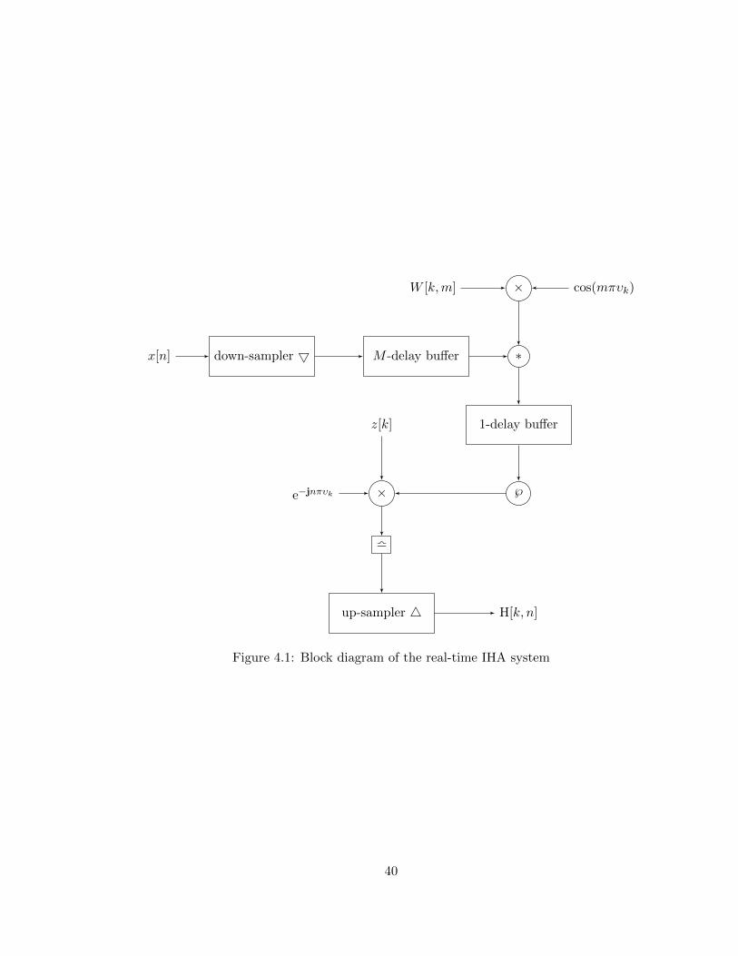
Fig. 4.1 presents the block diagram of our real-time IHA system. As illustrated, it
consists of two delay buffers, a total of M + 1 samples delay. The complexity of the above
construct in time and space is therefore O(Mn) and O(M), respectively (cf. [61, 56]).
Algorithm 1 specifies the implementation of the real-time system. The input signal x, in
this implementation, is represented by an input stream and is assumed to be zero-padded.
39
x[n] down-sampler M -delay buffer ∗
1-delay buffer
℘×e−jnπυk
z[k]
l
up-sampler H[k, n]
×W [k,m] cos(mπυk)
Figure 4.1: Block diagram of the real-time IHA system
40
Algorithm 2: The M + 1-delay fast online discrete IHA block
Input: k: the frequency index,x[n]: a stream of real numbers representing the input signal
Output: H[k, n]: a delayed stream of complex numbers representing the IHAtransform of x[n]
1 estimate M using (4.9)2 construct the window function W [k,m] using desired window (i.e. Blackman)3 construct the template signal: cos(mπυk)4 construct the filter: Fk ←W [k,m] · cos(mπυk)5 adjust zk using the template signal and the approach specified in 4.5.46 input x[n] using and M -delay buffer7 foreach x[n] do8 calculate the filter response using (4.10)9 estimate H[k, n] using a 1-delay buffer and the modified phasor construct in (4.11)
10 output H[k, n]
4.6 Summary
The IHA algorithm was formalized by using the decomposition scheme, presented in sec-
tion 2.2, and employing the phasor construct, specified in (4.8). The normalized frequency,
presented in the discretization section, makes the derivation independent of sampling fre-
quency. We provided a fast implementation of the IHA algorithm for being used in realtime
systems. The analysis of the algorithm will be provided in the chapter 7.
41
Chapter 5
Generalization into the Multi-
Dimensional Space
This chapter contributes to the instantaneous harmonic analysis of multi-dimensional
signals. A quaternion representation is proposed to support multiple phase elements.
The space is extended into hyper-complex in order to address multiple phase elements.
Hamilton’s quaternions are the extension of complex numbers into a higher dimen-
sion [53]. They are based on one real and three imaginary components represented by three
imaginary units such as i, j, and k where i2 = j2 = k2 = ijk = −1. Using the Cayley-
Dickson construct, quaternions can also be extended into hyper-complex numbers in which
each number consists of one real and 2M − 1 imaginary components where M > 2. Quater-
nions have been widely used by many researchers and they are reported in the literature
for the processing and representation of multidimensional data such as computer graphics,
computer aided geometry and design, signal processing, etc. Whilst they were introduced in
1843 by Hamilton, they have not been applied in signal processing until recent years [99]. In
42
signal processing, many quaternion applications can be found in time-frequency analysis of
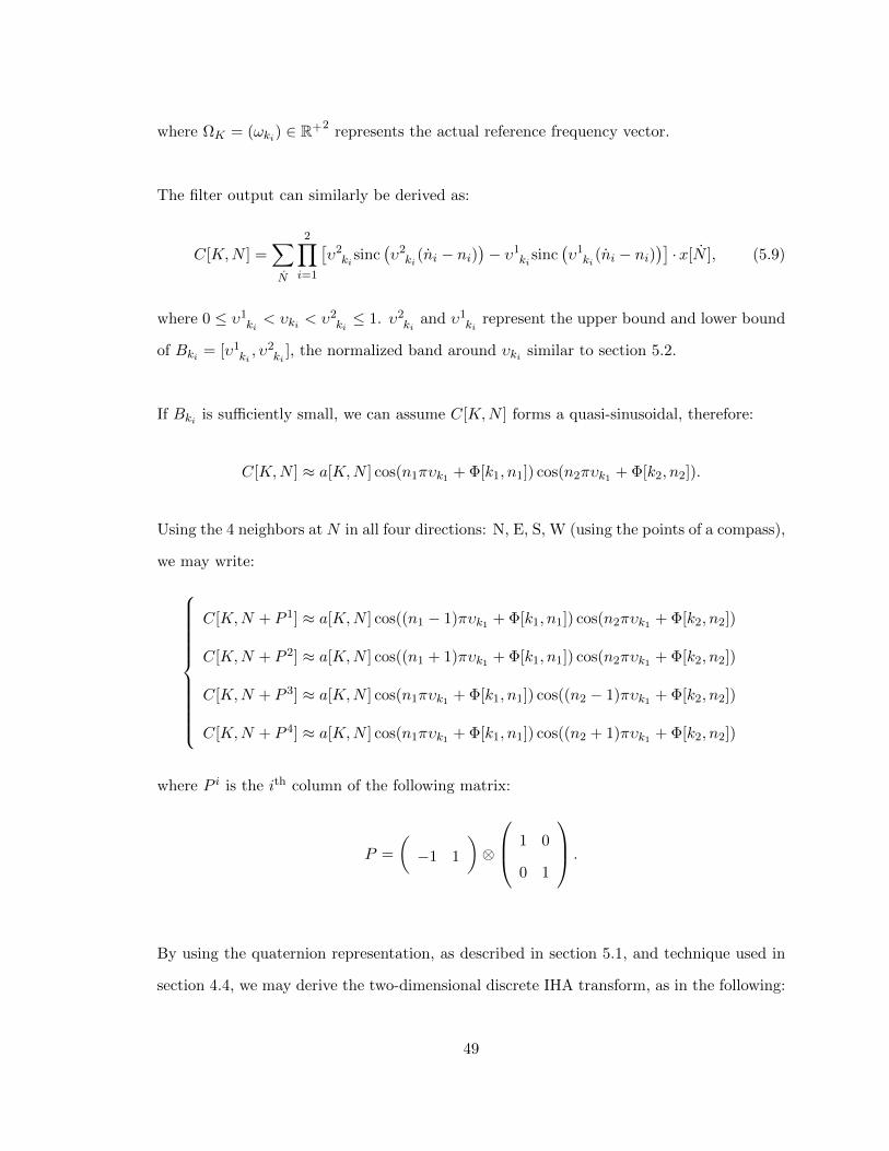
where P i is the ith column of the following matrix:
P =
−1 1
⊗
1 0
0 1
.
By using the quaternion representation, as described in section 5.1, and technique used in
section 4.4, we may derive the two-dimensional discrete IHA transform, as in the following:
49
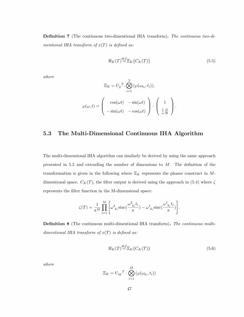
Definition 9 (The two-dimentional discrete IHA transform). The two-dimentional discrete
IHA transform of x[N ] is defined as:
H[K,N ]def= ΞKC[K,N ] (5.10)
where Ξ is the two-dimensional phasor construct:
ΞK(x[N ])def=
2i=1
e−j2i−1πυkm ·℘υk,i (x[N ]),
℘υ,i(x[N ])def=
j2i−1
sin 2πυ
e−πυj2i−1
−eπυj2i−1
T
·
x[N + P i1 ]
x[N + P i2 ]
,
P =
−1 1
⊗
1 0
0 1
,
and P i1 , Pi2 are the first and second elements of the ith row of the matrix P .
5.5 The Multi-Dimensional Discrete IHA Algorithm
The multi-dimensional discrete IHA algorithm may be derived by using a similar approach
in section 5.4 by extending the number of dimensions to M , as specified in the following:
Definition 10 (The multi-dimentional discrete IHA transform). The multi-dimentional
discrete IHA transform of x[N ] is defined as:
H[K,N ]def= ΞKC[K,N ] (5.11)
50
where Ξ is the multi-dimensional phasor construct:
ΞK(x[N ])def=
Mi=1
e−j2i−1πυkn ·℘υk,i (x[N ]),
℘υ,i(x[N ])def=
j2i−1
sin 2πυ
e−πυj2i−1
−eπυj2i−1
T
·
x[N + P i1 ]
x[N + P i2 ]
,P =
−1 1
⊗ IM ,
IM represents the identity matrix in M ×M , and P i1 , Pi2 are the first and second elements
of the ith row of the matrix P .
It can be shown that in case of M = 1, the above equation becomes (4.8)4.
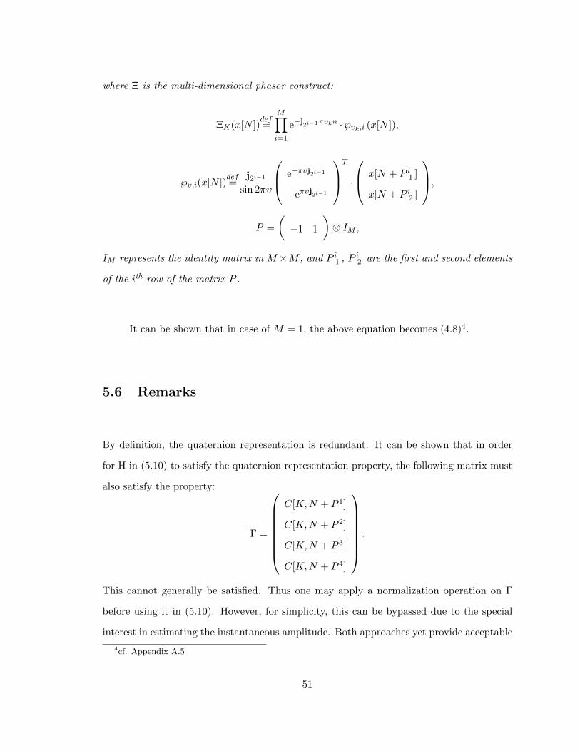
5.6 Remarks
By definition, the quaternion representation is redundant. It can be shown that in order
for H in (5.10) to satisfy the quaternion representation property, the following matrix must
also satisfy the property:
Γ =
C[K,N + P 1]
C[K,N + P 2]
C[K,N + P 3]
C[K,N + P 4]
.
This cannot generally be satisfied. Thus one may apply a normalization operation on Γ
before using it in (5.10). However, for simplicity, this can be bypassed due to the special
interest in estimating the instantaneous amplitude. Both approaches yet provide acceptable
4cf. Appendix A.5
51
results. Similar approach may be used in the M -dimensional case. The statement may
be generalized into the multi-dimensional space, in which case the quaternion property is
applied on all M(M −1)/2 combinations of every two dimensions i, j, which are used in the
calculations of ℘υ,i(x[N ]) and ℘υ,j(x[N ]), as specified in (5.11).
Although the IHA transform outperforms the QFT approach in terms of providing
the instantaneous amplitude and phase elements, the IHA algorithm cannot be used for
the multi-channel signals unless each channel is processed individually. The IHA transform
is quite similar to the quaternion wavelet transform in [24] in terms of using a redundant
representation. Our approach, however, outperforms the latter in terms of estimating the
instantaneous amplitude of the signal vs. the oscillating wavelet response. And finally, the
time complexity of the algorithm may be reduced by utilizing symmetric property of the
matrices.
52
Chapter 6
Generalization of IHA Algorithm
for Multiple Fundamental
Frequency Estimation
This chapter contributes to the generalization of the IHA algorithm by utilizing a com-
posite kernel. The generalized IHA algorithm contributes to the MFFE process. A
bottom-up overtone elimination approach is proposed by utilizing the representation of
the kernel function by a sequence of complex values. The generalized IHA algorithm
forms the core of our audio-to-MIDI system, which will be specified in chapter 8.
In this chapter, we generalize the IHA transform that was specified in chapter 4, by
utilizing a composite kernel function. Considering IHA to provide the instantaneous pure
components of the input signal, the generalized IHA estimates the instantaneous amplitude
and phase elements of the components based upon a generalized kernel function. Such
generalization makes it possible to use IHA in an MFFE process, where a multi-pitch
53
analysis is required for detecting multiple fundamental frequencies.
To overcome the harmonic collisions, several approaches may be used. Recently, Chen
and Liu used a modified harmonic product spectrum technique by calculating the magnitude
of the STFT for all the integer harmonics [26]. We propose using a bottom-up approach
in order to eliminate the overtones, as follows. In our model, the timbre is modeled by
a set of complex numbers, representing the amplification and phase lag of the subsequent
overtones, generated from the fundamental tone. Thus, starting from the lowest frequency,
the overtones are estimated and subsequently removed from the higher frequencies. Our
approach is sensitive to the fundamental frequencies while in [26] a product of the magnitude
of all integer harmonics is used.
In the following sections, the derivation of the generalized IHA algorithm by specifying
the properties of the kernel function and the constraints that are used in the decomposition
scheme is provided.
6.1 Overview
The IHA transform provides a decomposition framework for transforming an arbitrary signal
into a set of pure sinusoidals, given a set of reference frequencies. In here, we generalize the
kernel function ejt in (2.10), into a generic periodic function such that the input signal can
be decomposed into a set of composite components. Hence, the objective of the algorithm
is to generalize the kernel function ejt into a set of generic periodic functions ψ(t) such that
it can be used in the following decomposition scheme:
x(t) = ℜk
Hk(t)ψA(ωkt)+ r(t), (6.1)
54
where ψA(t) denotes the analytical form of ψ(t):
ψA(t) = ψ(t) + j ·Hψ(t),
H denotes the Hilbert transform, and r(t) represents a residual signal.
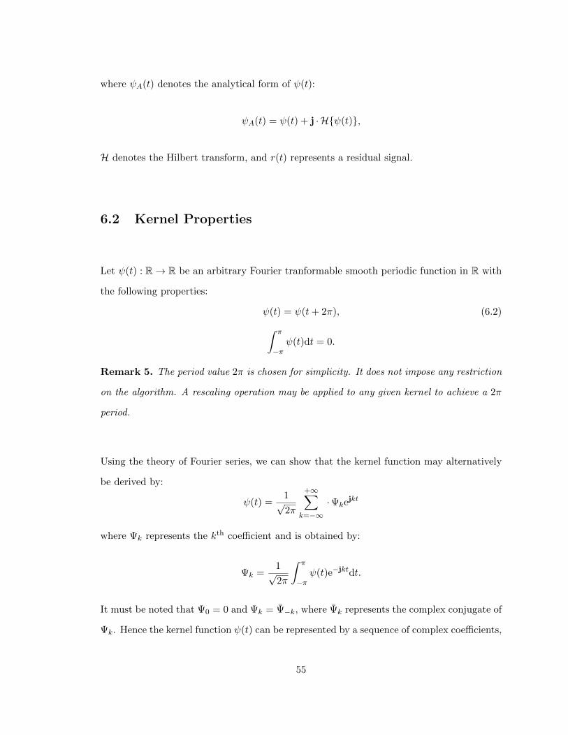
6.2 Kernel Properties
Let ψ(t) : R→ R be an arbitrary Fourier tranformable smooth periodic function in R with
the following properties:
ψ(t) = ψ(t+ 2π), (6.2) π
−πψ(t)dt = 0.
Remark 5. The period value 2π is chosen for simplicity. It does not impose any restriction
on the algorithm. A rescaling operation may be applied to any given kernel to achieve a 2π
period.
Using the theory of Fourier series, we can show that the kernel function may alternatively
be derived by:
ψ(t) =1√2π
+∞k=−∞
·Ψkejkt
where Ψk represents the kth coefficient and is obtained by:
Ψk =1√2π
π
−πψ(t)e−jktdt.
It must be noted that Ψ0 = 0 and Ψk = Ψ−k, where Ψk represents the complex conjugate of
Ψk. Hence the kernel function ψ(t) can be represented by a sequence of complex coefficients,
55
as the following:
(Ψk)∞k=1 .
6.3 Estimating the Kernel Function
Estimating the Kernel function from a sampled wave-form is a straightforward practice, as
kernels are represented by a series of complex coefficients Ψk, where k ∈ N. In practice, the
input wave-form is band-limited, and therefore, there exist an upper bound for k such that
k ≤ kmax.
Let ψ[k] represent sampled wave-form of the kernel ψ(t) with frequency f and sam-
pling frequency fs where fs ∈ N. Using sampling theorem, we can write:
ψ(2πft) =+∞
m=−∞ψ[m]sinc (fst−m) (6.3)
Since ψ is periodic, using (6.2), we can obtain:
ψ[m] = ψ(2πm
M), (6.4)
where m ∈ [0,M ], M ∈ N, and M = fsf .
For simplicity, f is assumed to be is a divisor of the sampling frequency. In general, a simple
interpolation technique may be applied by virtually choosing a new sampling frequency as:
fsnew = gcd(fsold, f),
where gcd represents the greatest common divisor.
56
Using (6.4), and by applying Fourier transform on both sides of (6.3), we obtain:
Fψ(2πft) = 1√2π
+∞n=−∞
M−1m=0
1
fsψ[m]e
−j(nM+m)ωfs , (6.5)
where 0 ≤ ω ≤ πfs.
Using (6.2), we can also derive the Fourier transform of ψ:
Fψ(2πft) =√2π
+∞k=−∞
Ψk · δ(ω − 2πfk), (6.6)
where 1 ≤ k ≤ M2 .
By equating (6.5) and (6.6), and using the limit theorem on ω → 2πfk, we can estimate
Ψk by:
Ψk =2
M
Mm=1
ψ[m] · e−j2πmk
M . (6.7)
The existence of inharmonicity in real audio signals makes the kernel estimation pro-
cess difficult. Inharmonicity is the measure to which the frequencies of the overtones do not
equate the integer multiples of the fundamental frequency. String instruments, for instance,
are known to produce imperfect harmonic tones. To overcome the inharmonicity issue, we
use a regression-based estimation algorithm, as specified in Alg. 3.
Although perfect harmonics are desirable, inharmonic sounds are not necessarily un-
pleasant. Among musicians, inhamonicity is sometimes referred to as the warmth property
of the sound. The topic has been researched in the audio processing field, especially in
sound synthesis [64].
57
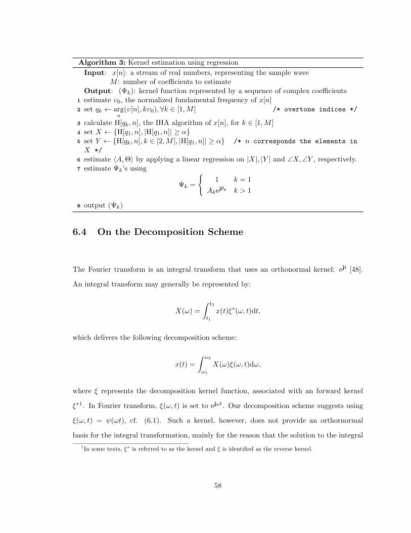
Algorithm 3: Kernel estimation using regression
Input: x[n]: a stream of real numbers, representing the sample waveM : number of coefficients to estimate
Output: (Ψk): kernel function represented by a sequence of complex coefficients1 estimate υ0, the normalized fundamental frequency of x[n]2 set qk ← arg
n(υ[n], kυ0),∀k ∈ [1,M ] /* overtone indices */
3 calculate H[qk, n], the IHA algorithm of x[n], for k ∈ [1,M ]4 set X ← H[q1, n], |H[q1, n]| ≥ α5 set Y ← H[qk, n], k ∈ [2,M ], |H[q1, n]| ≥ α /* n corresponds the elements in
X */
6 estimate ⟨A,Θ⟩ by applying a linear regression on |X|, |Y | and ∠X,∠Y , respectively.7 estimate Ψk’s using
Ψk =
1 k = 1
Akejθk k > 1
8 output (Ψk)
6.4 On the Decomposition Scheme
The Fourier transform is an integral transform that uses an orthonormal kernel: ejt [48].
An integral transform may generally be represented by:
X(ω) =
t2
t1
x(t)ξ∗(ω, t)dt,
which delivers the following decomposition scheme:
x(t) =
ω2
ω1
X(ω)ξ(ω, t)dω,
where ξ represents the decomposition kernel function, associated with an forward kernel
ξ∗1. In Fourier transform, ξ(ω, t) is set to ejωt. Our decomposition scheme suggests using
ξ(ω, t) = ψ(ωt), cf. (6.1). Such a kernel, however, does not provide an orthornormal
basis for the integral transformation, mainly for the reason that the solution to the integral
1In some texts, ξ∗ is referred to as the kernel and ξ is identified as the reverse kernel.
58
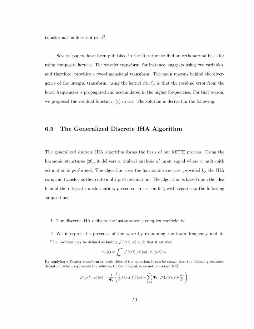
transformation does not exist2.
Several papers have been published in the literature to find an orthonormal basis for
using composite kernels. The wavelet transform, for instance, suggests using two variables,
and therefore, provides a two-dimensional transform. The main reasons behind the diver-
gence of the integral transform, using the kernel ψ(ωt), is that the residual error from the
lower frequencies is propagated and accumulated in the higher frequencies. For that reason,
we proposed the residual function r(t) in 6.1. The solution is derived in the following.
6.5 The Generalized Discrete IHA Algorithm
The generalized discrete IHA algorithm forms the basis of our MFFE process. Using the
harmonic structures [26], it delivers a timbral analysis of input signal where a multi-pith
estimation is performed. The algorithm uses the harmonic structure, provided by the IHA
core, and transforms them into multi-pitch estimation. The algorithm is based upon the idea
behind the integral transformation, presented in section 6.4, with regards to the following
suppositions:
1. The discrete IHA delivers the instantaneous complex coefficients;
2. We interpret the presence of the wave by examining the lower frequency and its
2The problem may be defined as finding J x(t), ψ such that it satisfies:
xA(t) =
∞
0+J x(t), ψ(ω) ·ψA(ωt)dω.
By applying a Fourier transform on both sides of the equation, it can be shown that the following recursivedefinition, which represents the solution to the integral, does not converge [108]:
J x(t), ψ(ω) = 1
Ψ1
1
2FxA(t)(ω)−
∞k=2
Ψk · J x(t), ψ(ωk)
.
59
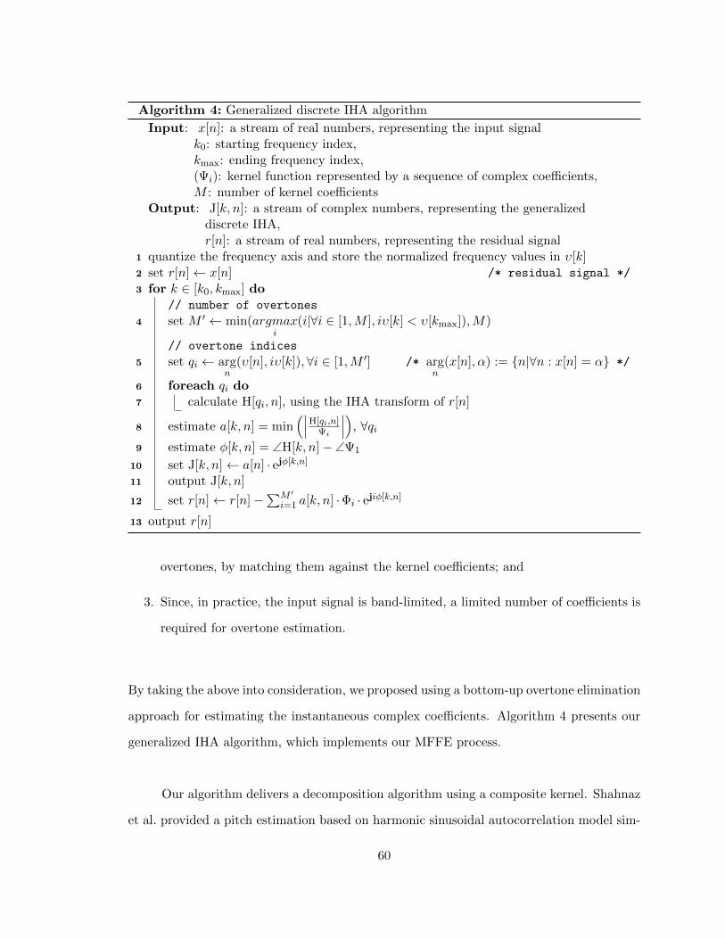
Algorithm 4: Generalized discrete IHA algorithm
Input: x[n]: a stream of real numbers, representing the input signalk0: starting frequency index,kmax: ending frequency index,(Ψi): kernel function represented by a sequence of complex coefficients,M : number of kernel coefficients
Output: J[k, n]: a stream of complex numbers, representing the generalizeddiscrete IHA,r[n]: a stream of real numbers, representing the residual signal
1 quantize the frequency axis and store the normalized frequency values in υ[k]2 set r[n]← x[n] /* residual signal */
3 for k ∈ [k0, kmax] do// number of overtones
4 set M ′ ← min(argmaxi
(i|∀i ∈ [1,M ], iυ[k] < υ[kmax]),M)
// overtone indices
5 set qi ← argn(υ[n], iυ[k]),∀i ∈ [1,M ′] /* arg
n(x[n], α) := n|∀n : x[n] = α */
6 foreach qi do7 calculate H[qi, n], using the IHA transform of r[n]
8 estimate a[k, n] = minH[qi,n]
Ψi
, ∀qi9 estimate φ[k, n] = ∠H[k, n]− ∠Ψ1
10 set J[k, n]← a[n] · ejφ[k,n]11 output J[k, n]
12 set r[n]← r[n]−M ′
i=1 a[k, n] ·Φi · ejiφ[k,n]
13 output r[n]
overtones, by matching them against the kernel coefficients; and
3. Since, in practice, the input signal is band-limited, a limited number of coefficients is
required for overtone estimation.
By taking the above into consideration, we proposed using a bottom-up overtone elimination
approach for estimating the instantaneous complex coefficients. Algorithm 4 presents our
generalized IHA algorithm, which implements our MFFE process.
Our algorithm delivers a decomposition algorithm using a composite kernel. Shahnaz
et al. provided a pitch estimation based on harmonic sinusoidal autocorrelation model sim-
60
ilar to our decomposition scheme in 2.2 [101]. Our approach delivers multi-pitch estimation
using composite kernels, which resembles the mother wave in wavelet transform. Also, Ding
et al. provided a pitch estimation using Harmonic Product Spectrum (HPS) [33]. The au-
thors used HPS as the product of spectral frames for constant number of overtones. Chen
and Liu utilized a modified HPS for multi-pith estimation [26]. Our method uses the kernel
coefficients Ψk’s in calculating the overtones.
6.6 Summary
We presented a signal decomposition algorithm using composite kernels. We used the
harmonic structure delivered by the IHA core and transformed them into multi-pitch infor-
mation. A bottom-up overtone reconstruction and elimination process was carried out for
the MFFE process. This forms the core of our audio-to-MIDI system, which is specified in
the chapter 8.
61
Chapter 7
Performance Analysis
This chapter presents the performance analysis of the presented IHA algorithm. A
new relation between CQT and WSFs is provided, in here. It is shown that CQT
can alternatively be implemented by applying a series of logarithmically scaled WSFs
while its window function is adjusted, accordingly. Both approaches yet provide a
short-time cross-correlation measure between the input signal and the corresponding
pure sinusoidal kernels whose frequencies are equal to the center of the filter band.
It is shown that the IHA phasor construct significantly improves the instantaneous
amplitudes estimation.
WSFs have been extensively used in the literature [103]. Both CQT andWSFs provide
a decomposition scheme based on a set of reference frequencies (cf. invertible CQT [56] and
the WSF decomposition, presented in section 4.5). In this chapter, we present a new relation
between CQT and WSFs. The derivation of the relation as well as the performance analysis
of our IHA algorithm are given in the following sections.
62
7.1 The Relation between CQT and WSF
We derive the relation between CQT and WSF by deriving a sliding version of CQT, by
using a delay operation [49]. The details are given in the following.
7.1.1 Deriving the Relation
Recall that the formal definition of CQT is given in a form of STFT, as presented in (2.1).
The sliding version of CQT may be formalized by using the following two assumptions:
1. x is zero padded;
2. and the STFT window is centered at n.
Thus:
X[k, n] =1
N [k]
N [k]−1m=0
W [k,m] · e−j2πQm
N [k] ·x[m+ n− N [k]− 1
2].
It must be noted that, by definition, N [k] is an odd number. Therefore, by substituting
N [k] with 2MK + 1, shifting m by −Mk, and also substituting
2Q
2Mk + 1
with υk using (4.6), we will have:
X[k, n] =(−1)Q
2Mk + 1
Mkm=−Mk
e−jπυkm ·x[m+ n] ·W [k,m+Mk].
63
Without losing generality, we can rewrite the window W [k,m +Mk] as W [k,m], where m
is shifted by Mk. Therefore,
X[k, n] = ξ
x, ejπυkm,
(−1)Q
2Mk + 1·Wk[m]
, (7.1)
where ξ denotes the windowed cross-correlation, as defined in the following:
ξ(x, τ,W ) =M
m=−Mx[n−m] · τ [m] ·W [m], (7.2)
and W is a symmetric window with 2M + 1 samples in length.
Corollary 1. Eq. (7.1) suggests that CQT is equivalent to the cross correlation of the
input signal with the sinusoidal kernel cos(πυkm) in its analytical form within the following
window:
(−1)Q
2Mk + 1·Wk[m].
Similarly, (4.10) can be derived by means of the above cross-correlation. By choosing:
Mk =2
λυk,
we may derive C[k, n] as:
C[k, n] = ξ
x, cos(πυkm),
2
Mksinc
m
Mk
·Wk[m]
. (7.3)
Thereby:
Corollary 2. We interpret (7.3) as the cross-correlation of the input signal with the sinu-
soidal kernel cos(πυkm) within the window:
2
Mksinc
m
Mk
·Wk[m].
64
Hence, by comparing (7.1) and (7.3), it can be deduced that:
Corollary 3. CQT is the equivalent of performing a series of WSF whose bandwidths
correspond to (2.6), where
λ =2
Q,
and the window function is adjusted by the following:
Wsinc[m] = (−1)Q ·4Mk + 2
Mk
· sinc
m
Mk
·WCQT[m].
By assuming that Q is generally an even number, and Mk is also considerably large, the
above adjustment may be simplified as:
Wsinc[m] = 4sinc
m
Mk
·WCQT[m]. (7.4)
Corollary 4. CQT and WSF can interchangeably be used as both provide a cross-correlation
measure of the function with a sinusoidal kernel.
7.1.2 Interpretation
The decomposition scheme presented in section 2.2 makes it possible to perform an IHA
of the input signal. This was achieved by estimating the complex values H[k, n]’s which
designate the phasor representation of the instantaneous amplitude and phase lag of the
signal’s constituent components. Both CQT and our presented WSF provide instantaneous
complex values, which can be used in such estimation.
One interesting property of CQT’s complex kernel e−jπυkm is that the magnitude
of the resulting transformation can be interpreted as a representation for instantaneous
65
amplitudes of the corresponding components. At first glance, it may seem that the WSF
approach lacks such a property. However, to resolve this, one may simply substitute the
cos(πυkm) kernel with its analytical form:
τ [m] = e−jπυkm,
without changing the relation. Such WSF will be equivalent to performing the filters on
the analytical form of the input signal using Hilbert transform. Since we demonstrated
the sliding CQT could be derived by means of WSF, an invertible CQT is achievable, and
thereby, a reconstruction algorithm may be used, cf. (2.10).
Fig. 7.1 presents a sample output of the IHA algorithms using flat and Blackman
windows in 7.1(a) and 7.1(b), respectively. A single-component piece-wise sinusoidal with
unit amplitude and frequency of 880 Hz has been used. The sampling frequency were also
44 kHz. In order to condense the temporal window as much as possible, γ = 2 was used.
Table 7.1 summarizes the overall instantaneous amplitude estimation rate. The overall rate
has been estimated by averaging the absolute values of distances between estimated and
actual amplitudes. The ratio of the signal length over latency, as well as the latency itself
were 2.20 and 2.30× 10⁻³, respectively. In this particular example, IHA delivered a stabi-
lized estimate even though the underlying filtering algorithm provided unstable oscillating
response, cf. WSF-IHA flat vs. WSF Blackman.
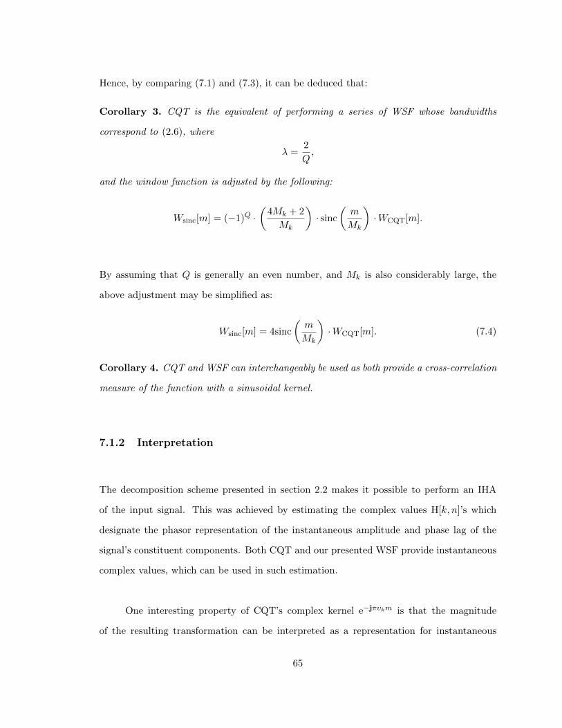
In Fig. 7.2, a sample output for a two-component input signal using a semi-tone
bandwidth and Blackman Window has been demonstrated. The details are given in Table
7.2, correspondingly. In both examples, it is shown that using the combination of WSF and
IHA not only maximizes the estimation rate, but also minimizes the overall reconstruction
error.
66
0 0.002 0.004 0.006 0.008 0.010
.5
1
1.5
time (s)
ampl
itude
actualCQTWSFCQT+IHAWSF+IHA
(a) flat window
0 0.002 0.004 0.006 0.008 0.010
.5
1
1.5
time (s)
ampl
itude
actualCQTWSFCQT+IHAWSF+IHA
(b) Blackman window
Figure 7.1: Sample output of CQT vs. WSF and IHA
67
0 0.12 0.24 0.36 0.48 0.60
.5
1
1.5
time (s)
ampl
itude
actualCQTWSFCQT+IHAWSF+IHA
(a) first component
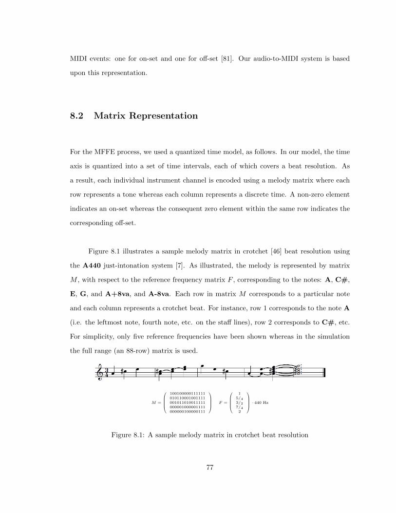
0 0.12 0.24 0.36 0.48 0.60
.5
1
1.5
time (s)
ampl
itude
actualCQTWSFCQT+IHAWSF+IHA
(b) second component
Figure 7.2: Sample output of two-component signal using a semitone bandwidth
68
MethodOverall Estimation Rate
flat-window Blackman-window
Amp. Rec. Amp. Rec.
CQT 88.20 87.24 46.28 65.54
WSF 83.12 86.00 76.73 83.52
CQT+IHA* 88.26 87.24 46.30 65.54
WSF+IHA* 83.28 86.00 76.78 83.52
CQT+IHA 88.11 89.68 93.06 95.68
WSF+IHA 92.03 95.01 94.18 96.39
Amp. amplitude response
Rec. signal reconstruction
* not using eq. (4.11)
Table 7.1: Overall estimation rate for instantaneous amplitude and full signal reconstructionof a sample signal using CQT, WSF and IHA.
MethodOverall Estimation Rate
Amp.Rec.
C1 C2 C1 + C2
CQT 60.75 63.36 55.20 53.78
WSF 79.55 83.07 81.31 82.46
CQT+IHA 88.18 93.31 87.41 92.03
WSF+IHA 90.02 94.25 89.26 93.45
Table 7.2: Overall estimation rate for instantaneous amplitude and full signal reconstructionof a two-component signal
Although CQT was originally defined by means of STFT [16], a number of versions
of it have been used in the literature. For instance, Graziosi et al. utilized a sliding filter
bank approach to calculate the CQT [49] while Holighaus et al. [56] proposed using a sliced
version. In their approach the input signal is uniformly sliced and consequently converted
into a set of atom coefficients. Since those coefficients can form a matrix, they proposed
obtaining the reconstructed signal using a pseudo-inverse approach.
Such matrix representation seems to be highly efficient for signal registration and
compression. Nagathil and Martin,for instance, provided an optimal signal reconstruction
69
from constant-Q spectrum [84]. However, depending on the application, other representa-
tion schemes may be also used. For example, in melody extraction, one major concern is
the detection of on-set/off-set events, which can be achieved by processing an instantaneous
amplitude response. In such a model, whether a linear centric or a logarithmic centric ap-
proach is used, the sliding transformation is always invertible (cf. (2.6) and (2.7)). The
window function, however, produces an small noise, cf. [103].
7.2 Relation to Wavelets
An interesting property of logarithmic quantization is that the resulting filter outputs inherit
wavelet properties. For instance, in case of octave bandwidth (λ = 2), the filter output
simulates a quasi-Shannon wavelet:
Ck(t) =1
π
ωk
π√2·WTψ(Sha)x
π√2
ωk, t
. (7.5)
In the above equation, WTψ(Sha)x represents the continuous wavelet transform of x
using Shannon wavelet [75] with
π√2
ωk, t,
as the scale and translational values, respectively. Choosing a lower value for λ results
in a higher Q factor and therefore provides rational dilation wavelets [9]. Although the
wavelet output is rescaled by a factor of√ωk, both approaches provide full reconstruction
algorithms.
Although ωk’s are logarithmically scaled, (2.6) shows that they are yet linearly cen-
tered within the bands. This poses certain restrictions in practice, especially in music
analysis, where the border frequencies are also desired to be logarithmically scaled, i.e.
70
(2.7). The border frequencies are referred to the upper-bound and the lower-bound of Bk.
CQT suggests that Q is integer. However, in order to have side-by-side bandwidths, a
real-valued Q must be used in general. Moreover, a lower bound for Q may also be derived
as Q > 1, due to the fact that in case Q = 1, the quantization of the frequency axis by non-
overlapping frequency bands is not possible, as the minimal frequencies of all Bk’s approach
zero.
Fig. 7.3 demonstrates the distance between the center frequency and the upper and
lower border frequencies in form of musical intervals. As illustrated, for lower values of
Q, the difference between the minimal and maximal frequencies is considerably large (i.e.
octave vs. perfect fifth, at Q = 2). However, as Q approaches 34, both values merge into
a semitone, which makes the filter banks suitable for a 12-equal temperament system im-
plementation [7]. Therefore, for Q > 34, the two linear-and logarithmic-centric approaches
merge (cf. (2.7), (2.6)).
0 4 8 12 16 20 24 28 32
semi−tonetone
min 3rdMaj 3rd
4th
5th
8va
Q
inte
rval
lowerupper
Figure 7.3: Lower-limit vs. upper-limit intervals of various Q’s
71
7.3 Simulations
The performance analysis of the CQT in (7.1) against WSF with and without using window
functions is provided here. A Blackman window is used in this comparison. We apply the
IHA phasor construct on the real-part of the CQT output as well as the WSF approach.
The details are given in the following.
In order to evaluate the relation in (7.4), we examined the performance of the CQT
in (7.1) against WSF with and without using window functions. A Blackman window was
used in the experiment. We also applied our phasor construct on the real-part of the CQT
output as well as the WSF approach for the instantaneous harmonic analysis. The details
are given in the following.
In the simulations, we used two sets of synthetic data as well as one set of mid-range
real-audio. We applied the algorithms on the frequency range between 110 and 1, 760Hz
with semitone steps, resulting in full four octaves. Both CQT and WST using Blackman
window along with IHA were applied to the data sets.
We calculated the overall amplitude estimation success rate for the two synthetic data
sets with respect to the actual amplitudes. The threshold value, as explained in section 4.5.4,
was set to one-tenth of the maximum amplitude and was applied to all four methods. The
following formula was used for calculating the success rate:
rate = 100×
1− 1
N
k,n
|a[k,n]−a[k,n]|a[k,n]
, a[k, n] = 0,
where a and a denote the actual and estimated amplitudes, respectively. The summary of
the results is given in table 7.3.
72
MethodOverall Estimation RateDS1 DS2
CQT 43.51 31.87
WSF 70.35 51.26
CQT+IHA 79.87 55.69
WSF+IHA 82.28 57.75
Table 7.3: Overall estimation rate on synthetic data
In the case of real audio data, since the actual amplitudes were unknown, we calculated
the reconstruction rate, using a weighted averaging method as given in the following:
rate = 100×
1−
n|x[n]− x[n]| · |xA[n]|
max(|xA[n]|) ·n|xA[n]|
,
where x, x, and xA denote the original, estimated, and analytical signals, respectively. In
our experiment we modified the signals by applying a low pass filter in order to eliminate
the frequencies above 1, 760Hz. The results are shown in table 7.4.
MethodOverall Estimation Rate
DS3*
CQT 86.47
WSF 89.72
CQT+IHA 90.03
WSF+IHA 90.27
* modified
Table 7.4: Overall reconstruction rate on real audio signals
Tables 7.3 and 7.4 demonstrate that WSF, in general, outperformed CQT in both
amplitude estimation as well as signal reconstruction. The combination of IHA and WSF
significantly improves the amplitude estimation and reduces the overall reconstruction error.
73
7.4 Summary
A new relation between CQT and WSF in the presented continuous model was provided.
The invertibility of our IHA was discussed. We demonstrated that the performance of CQT
can be enhanced by adjusting its window function, as specified in (7.4). Our simulation
results supported the theory. In the following chapters we examine the applicability of the
IHA algorithm for improving the MFFE and note on-set/off-set detection processes.
74
Chapter 8
The Transcription System
This chapter contributes to the post-processing algorithms, used in the proposed tran-
scription system. The output of the MFFE process using the generalized IHA algorithm
is translated into note on-set/off-set events. The specification of our proposed audio-to
-MIDI system as well as the note event representation, used in the simulation, are also
discussed here.
The music transcription in this thesis is defined as a process of analyzing audio signals
in order to detect on-set/off-set events of the notes, in form of an audio-to-MIDI practice.
Percussion analysis or processing of musical accidentals is not included (cf. [71, 10]). Our
proposed transcription system is built on top of the generalized IHA transform, which was
presented in the previous chapters. It is based upon the note events modeling, which is
specified in the following.
In the following sections, an overview of the note events modeling is given; an equiv-
alent matrix representation is provided; the proposed transcription system is specified; the
75
MFFE process is reviewed; and the post-processing algorithms for extracting the note events
are provided. The simulation results are provided.
8.1 An Overview of Note Events Modeling
The music notations deliver three primary pieces of information: beat information, note
events, and instrumentation:
1. the beat information specifies how the note events are translated in time;
2. the note events provide the information about note on-sets and off-sets;
3. and the instrumentation represents the information about the tone color, also known
as timbre.
Given the beat information, a piece of music may be encoded using a set of tuples, as
specified in the following. Coding and synthesis of articulations are out of the scope of our
discussion.
One important characteristic of the MIDI format is that the MIDI data is represented
in time rather than beats. Therefore, we exclude the beat information from the note event
representation. Hence, we use a set of 5-tuples ⟨i, n, v, ton, toff⟩ where i represents the
instrument index, n represents the note index, v represents the loudness, ton represents the
on-set, and toff represents the off-set. The note index is associated with a fundamental
frequency. The loudness factor in the MIDI context is also referred to as the velocity [81].
In some context, toff is substituted with note duration. Translating such representation
into MIDI format is a straightforward process. Each tuple is translated into two individual
76
MIDI events: one for on-set and one for off-set [81]. Our audio-to-MIDI system is based
upon this representation.
8.2 Matrix Representation
For the MFFE process, we used a quantized time model, as follows. In our model, the time
axis is quantized into a set of time intervals, each of which covers a beat resolution. As
a result, each individual instrument channel is encoded using a melody matrix where each
row represents a tone whereas each column represents a discrete time. A non-zero element
indicates an on-set whereas the consequent zero element within the same row indicates the
corresponding off-set.
Figure 8.1 illustrates a sample melody matrix in crotchet [46] beat resolution using
the A440 just-intonation system [7]. As illustrated, the melody is represented by matrix
M , with respect to the reference frequency matrix F , corresponding to the notes: A, C#,
E, G, and A+8va, and A-8va. Each row in matrix M corresponds to a particular note
and each column represents a crotchet beat. For instance, row 1 corresponds to the note A
(i.e. the leftmost note, fourth note, etc. on the staff lines), row 2 corresponds to C#, etc.
For simplicity, only five reference frequencies have been shown whereas in the simulation
DS5: full-range multi instrument. The details of the datasets are provided in Appendix B.
The MIDI parts were extracted and synthesized using three timbre banks. The data items
were created by splitting the original files into five-measure segments. The accidentals were
not used during the synthesizing process. The algorithm was applied to individual segments
and the overall accuracy was calculated for each data set. In our experiment a maximum
of two overtones was used. The result is listed in table 8.1. Notes below C3 were not used
in the simulation.
Accuracy AP 0-overtone 1-overtone 2-overtone
DS1 1.9 99.5 98.3 97.2
DS2 2.7 99.8 98.8 98.3
DS3 4.0 99.4 97.8 97.8
DS4 2.6 91.1 88.0 78.6
DS5 3.2 81.3 76.8 72.5
AP Average Polyphony
Table 8.1: Overall AMT Simulation Results
In the above table, the melody matrix was used as the ground truth. Our accuracy
measurement supports the Music Information Retrieval Evaluation eXchange (MIREX)
specification [83]. MIREX specifications define the accuracy of note event detection as the
following:
1. The onset is detected within a ±50 ms range of a ground-truth onset
83
2. and the detected F0 is within a quarter tone of the ground-truth pitch
8.7 Summary
The applicability of the generalized IHA algorithm in MFFE and note event modeling
was demonstrated. An audio-to-MIDI transcription system based on generalized IHA was
presented.
While the transcription output seems satisfactory for mid-range and slow pieces (DS1
-3), our simulation shows that the accuracy has been decreased by 25% in the case of using
full-range data. Such errors occur mainly for the following reasons: the response latency
associated with the low frequencies, the difference between the responses from the funda-
mental tone and the overtones, and the harmonic collision. The existence of inharmonicity
in real audio signals, where the frequencies of the overtones do not follow the integer mul-
tiples of the fundamental frequency, makes the transcription process rather difficult.
84
Algorithm 5: Algorithm for generating note events
Input: i: instrument index,τ : tempo (in crotchets per minute),u: beat resolution (in whole note unit),T : sampling frequency,J[k, n]: a stream of complex numbers, representing the generalized discreteIHAk0: starting frequency index,kmax: ending frequency index,ϵ: amplitude threshold
Output: e: collection of ⟨b, k, l⟩ representing the note events where b ∈ N, k ∈ Z,and l ∈ N represent the beat index, the note index, and the velocity level.(l = 0 denotes off-set)
1 construct the melody matrix M by performing a down-resolution on every row of Jusing the ratio r, where J[k, n] ≥ ϵ where
r =
1
T
: τ
240u
2 set e← 3 M ←M : mi,j ≥ ϵ /* eliminate the noisy output */
4 O ← sgn(mi,j −mi,j−1) where sgn represent the signum function /* on-set */
5 F ← sgn(mi,j+1 −mi,j) /* off-set, in binary level */
6 for k ∈ [k0, kmax] do7 for b ∈ [0, bmax] do8 if Ok,n ≥ 0 then9 add ⟨b, k,Ok,n⟩ to e
10 if Fk,n ≤ 0 then11 add ⟨b, k, 0⟩ to e
12 output e[n]
85
Chapter 9
Conclusions and Future Directions
Techniques and challenges regarding both time-frequency analysis and auto-
matic music transcription were reviewed. A novel approach for estimating the
instantaneous amplitude and phase elements of real-valued signals based on en-
hanced Constant-Q filtering and a unique phasor construct was presented. It
was demonstrated that the proposed algorithm delivers a stable estimation by
maintaining the instantaneous amplitudes and the phase lags locally constant.
The magnitude of such a construct provides a finer estimate for instantaneous
amplitude, compared to the analytical kernel that is used in CQT.
A fast real-time M +1-delay IHA algorithm was implemented. A generalization
of the IHA algorithm for multi-dimensional signal analysis was also formalized in
the hyper-complex space. A quaternion representation was proposed to support
multiple phase elements.
86
A theoretical analysis of the IHA algorithm was provided. A new relation be-
tween the CQT and WSFs based on the original signal model in the continuous
form was presented. It was shown that CQT can alternatively be implemented
by applying a series of logarithmically scaled WSFs while its window function
is adjusted, accordingly. Both approaches yet provide a short-time cross-corre-
lation measure between the input signal and the corresponding pure sinusoidal
kernels whose frequencies are equal to the center of the filter band. It was
shown that the IHA phasor construct significantly improves the instantaneous
amplitude estimation.
A generalization of the IHA algorithm was provided by utilizing composite ker-
nels for timbral analysis. The IHA algorithm contributed to an MFFE process
where a post-processing overtone elimination algorithm was used. Due to the
limited number of overtones in practice, a representation of the kernel function
by a sequence of complex values was used.
An audio-to-MIDI system was designed based upon the generalized IHA algo-
rithm. The proposed system was implemented using the generalized IHA algo-
rithm as the MFFE block and a set of post-processing algorithms for detecting
the note on-set/off-set events. By using the timbral data captured by an offline
process, the generalized IHA provides a set of sequences of complex coefficients,
designating the presence of notes in time.
The performance of the proposed audio-to-MIDI system was analyzed by apply-
ing the algorithms on five data sets: treble-range, full-range, four-part choral,
full-range piano, and full-range multi instrument. The MIDI parts were ex-
tracted and synthesized using timbre banks. The algorithm was applied to each
87
individual segment and the overall accuracy was measured for each data set.
The data sets were explicitly selected to examine the performance of our MFFE
algorithm with regards to latency, amplitude weighting, and harmonic collision.
Our simulation demonstrated compelling results, with regards to the MIREX
specification and existing state-of-the-art AMT systems, as reported in the lit-
erature [83].
The latency factor, especially in the lower frequency range imposes a risk where
a low beat resolution is desired. While it can be assumed that, in practice,
no consecutive low-range tones coexist simultaneously, a lower quality factor
resulting in overlapping bands (i.e. 200- or 400-cent width) may be used for
very low range tones. A post-processing selection algorithm, such as maximum
likelihood, may be used to classify best candidates among the neighbored bins
[72].
One of the interesting extensions of the proposed algorithm is to utilize the
algorithm in interactive music retrieval systems such as humming. The IHA al-
gorithm may also be used in music registration and classification systems, with
regards to the provided normalized temporal spectral analysis. Another inter-
esting extension would be to evaluate the performance of the multi-dimentional
IHA and its applicability to multi-dimensional signals.
The proposed algorithms can be used as a basis for improving existing transcrip-
tion systems. The ability of the IHA algorithm to simultaneously decompose
an audio input into its fundamental components and deliver their instantaneous
amplitudes, makes it exceptionally beneficial in music processing applications.
The IHA algorithm may be applied in various AMT sub-systems such as note
88
tracking, chord analysis, we well as instrument identification.
During recent years, many contributed to individual areas of AMT. Although
there have been significant improvements in the state-of-the-art AMT tech-
niques, the overall performance of the existing systems is yet not comparable to
human experts [11]. AMT is essentially a complex problem and requires various
techniques. It is still an open problem, especially in the field of polyphonic tran-
scription, and requires experts from different disciplines. Although the number
of components that are possibly required to implement a functional AMT sys-
tem is beyond the scope of this thesis, we hope our fundamental contributions
to the harmonic analysis motivate future research directions.
89
Bibliography
[1] Abdallah, S. A. and Plumbley, M. D. [2003], Probability as metadata: Event detection
in music using ICA as a conditional density model, in ‘4th International Symposium
on Independent Component Analysis and Blind Signal Separation (ICA2003)’, Nara,
Japan, pp. 223–238.
[2] Abe, M. and Ando, S. [1995], Nonlinear time-frequency domain operators for decom-
posing sounds into loudness, pitch and timbre, in ‘International Conference on Acous-
tics, Speech, and Signal Processing, ICASSP-95’, Vol. 2, pp. 1368–1371.
[3] American Institute of Physics, Acoustical Society of American Standards & Secretariat
and American National Standards Institute [2001, Revised in 2011], ANSI/ASA S1.42–
2001 (R2011): American National Standard, Design Response of Weighting Networks
for Acoustical Measurements, Acoustical Society of America standards, American In-
stitute of Physics, Melville, N.Y., USA.
[4] Argent, F., Nesi, P. and Pantaleo, G. [2011], ‘Automatic transcription of polyphonic
music based on the constant-Q bispectral analysis’, IEEE Transactions on Audio,
Speech, and Language Processing 19(6), 1610–1630.
[5] Arroabarren, I., Rodet, X. and Carlosena, A. [2006], ‘On the measurement of the
instantaneous frequency and amplitude of partials in vocal vibrato’, IEEE Transactions
on Audio, Speech, and Language Processing 14(4), 1413–1421.
90
[6] Balazs, P., Dorfler, M., Jaillet, F., Holighaus, N. and Velasco, G. A. [2011], ‘Theory,
implementation and applications of nonstationary gabor frames’, Computational and
Applied Mathematics 236(6), 1481–1496.
[7] Barbour, J. M. [1951], Tuning and Temperament: A Historical Survey, Michigan State
College Press, Michigan, USA.
[8] Bari, N. K. [1964], A Treatise on Trigonometric Series [Vols. I & II], Pergamon Press.
[9] Bayram, I. and Selesnick, I. W. [2009], ‘Frequency-domain design of overcom-
plete rational-dilation wavelet transforms’, IEEE Transactions on Signal Processing
57(8), 2957–2972.
[10] Benetos, E. [2012], Automatic Transcription of Polyphonic Music Exploiting Temporal
Evolution, PhD thesis, School of Electronic Engineering and Computer Science, Queen
Mary University of London.
[11] Benetos, E. and Dixon, S. [2013], ‘Multiple-instrument polyphonic music transcription
using a temporally constrained shift-invariant model’, The Journal of the Acoustical
Society of America 133(3), 1727–1741.
[12] Bertin, N., Badeau, R. and Richard, G. [2007], Blind signal decompositions for auto-
matic transcription of polyphonic music: Nmf and k-svd on the benchmark, in ‘IEEE
International Conference on Acoustics, Speech and Signal Processing (ICASSP 2007)’,
Vol. 1, pp. I–65–I–68.
[13] Bertin, N., Badeau, R. and Vincent, E. [2010], ‘Enforcing harmonicity and smoothness
in bayesian non-negative matrix factorization applied to polyphonic music transcrip-
tion’, IEEE Transactions on Audio, Speech, and Language Processing 18(3), 538–549.
[14] Boashash, B. [1992a], ‘Estimating and interpreting the instantaneous frequency of a
signal, part i: Fundamentals’, Proceedings of the IEEE 80(4), 520–538.
91
[15] Boashash, B. [1992b], ‘Estimating and interpreting the instantaneous frequency of a
signal, part ii: Algorithms and applications’, Proceedings of the IEEE 80(4), 540–568.
[16] Brown, J. [1991], ‘Calculation of a constant-q spectral transform’, The Journal of the
Acoustical Society of America 89(1), 425–434.
[17] Bruno, I. and Nesi, P. [2005], ‘Automatic music transcription supporting different
instruments’, Journal of New Music Research 34, 139–149.
[18] Cancela, P., Rocamora, M. and Lopez, E. [2009], An efficient multi-resolution spectral
transform for music analysis, in ‘Proceedings of the 10th International Society for
Music Information Retrieval Conference (ISMIR 2009)’, Kobe, Japan, pp. 309–314.
[19] Carleson, L. [1966], ‘On convergence and growth of partial sums of Fourier series’, Acta
Mathematica 116(1), 135–157.
[20] Casazza, P. G. [2000], ‘The art of frame theory’, Taiwanese Journal Mathematics
4, 129–202.
[21] Cemgil, A. T. [2004], Bayesian Music Transcription, PhD thesis, Radboud University
of Nijmegen.
[22] Cemgil, A. T. and Kappen, B. [2003], ‘Monte Carlo methods for tempo tracking and
rhythm quantization’, Journal of Artificial Intelligence Research 18, 45–81.
[23] Chafe, C. and Jaffe, D. [1986], Source Separation and Note Identification in Polyphonic
Music, in ‘Proceeding of the IEEE International Conference on Acoustics, Speech, and
Signal Processing (ICASSP)’, Tokyo, pp. 1289–1292.
[24] Chan, W. L., Choi, H. and Baraniuk, R. [2004a], Quaternion wavelets for image analysis
and processing, in ‘International Conference on Image Processing (IICIP’04)’, Vol. 5,
pp. 3057–3060.
92
[25] Chan, W. L., Choi, H. and Baraniuk, R. G. [2004b], Directional hypercomplex wavelets
for multidimensional signal analysis and processing, in ‘IEEE International Conference
on Acoustics, Speech, and Signal Processing (ICASSP’04)’, Vol. 3, pp. iii–996–999.
[26] Chen, X. and Liu, R. [2013], Multiple pitch estimation based on modified harmonic
product spectrum, in ‘Proceedings of the 2012 International Conference on Informa-
tion Technology and Software Engineering’, Vol. 211 of Lecture Notes in Electrical
Engineering, Springer Berlin Heidelberg, pp. 271–279.
[27] Chuan, C.-H. and Chew, E. [2005], Polyphonic audio key finding using the spiral
array CEG algorithm, in ‘IEEE International Conference on Multimedia and Expo
(ICME’05)’, pp. 21–24.
[28] Cohen, L. [1994], The uncertainty principle in signal analysis, in ‘Proceedings of
the IEEE-SP International Symposium on Time-Frequency and Time-Scale Analysis’,
pp. 182–185.
[29] Costantini, G., Todisco, M. and Saggio, G. [2011], A sensor interface based on sparse
nmf for piano musical transcription, in ‘4th IEEE International Workshop on Advances
in Sensors and Interfaces (IWASI’11)’, pp. 157–161.
[30] Cranitch, M., Cychowski, M. T. and FitzGerald, D. [2006], Towards an inverse
constant-Q transform, in ‘120th Audio Engineering Society Convention’, pp. 1–5.
[31] da C. B. Diniz, F., Biscainho, L. and Netto, S. [2007], Practical design of filter banks for
automatic music transcription, in ‘5th International Symposium on Image and Signal
Processing and Analysis (ISPA’07)’, pp. 81–85.
[32] de Cheveigne, A. and Kawahara, H. [2002], ‘YIN, a fundamental frequency estimator
for speech and music’, The Journal of the Acoustical Society of America 111(4), 1917–
1930.
93
[33] Ding, H., Qian, B., Li, Y. and Tang, Z. [2006], A method combining lpc-based cep-
strum and harmonic product spectrum for pitch detection, in ‘Proceedings of the 2006
International Conference on Intelligent Information Hiding and Multimedia’, IIH-MSP
’06, IEEE Computer Society, Washington, DC, USA, pp. 537–540.
[34] dos Santos, C. N., Netto, S. L., Biscainho, L. W. P. and Graziosi, D. B. [2004], A
modified constant-Q transform for audio signals, in ‘IEEE International Conference on
Acoustics, Speech, and Signal Processing (ICASSP’04)’, Vol. 2, pp. ii–469–472.
[35] Ehmann, A. F. [2010], High-Resolution Sinusoidal Analysis for Resolving Harmonic
Collisions in Music Audio Signal Processing, PhD thesis, University of Illinois at
Urbana-Champaign.
[36] Eldar, Y. and Michaeli, T. [2009], ‘Beyond bandlimited sampling’, Signal Processing
Magazine, IEEE 26(3), 48–68.
[37] Fan, Z., Sufen, D., Guifa, T. and Jie, Y. [2010], Improved humming music retrieval
method based on wavelet transformation and dynamic time warping, in ‘International
Conference on Internet Technology and Applications’, pp. 1–4.
[38] Farhat, H. [1990], The Dastgah Concept in Persian Music, Cambridge University Press.
[39] Feng, W. and Hu, B. [2008], Quaternion discrete cosine transform and its application
in color template matching, in ‘Congress on Image and Signal Processing (CISP ’08)’,
Vol. 2, pp. 252–256.
[40] Fitch, J. and Shabana, W. [1999], A wavelet-based pitch detector for musical signals,
in ‘Proceedings of 2nd COST-G6 Workshop on Digital Audio Effects (DAFx99)’, Nor-
wegian University of Science and Technology, Trondheim, pp. 101–104.
[41] Folland, G. B. and Sitaram, A. [1997], ‘The uncertainty principle: a mathematical
survey’, Journal of Fourier Analysis and Applications pp. 207–238.
94
[42] Fuentes, B., Liutkus, A., Badeau, R. and Richard, G. [2012], Probabilistic model for
main melody extraction using constant-Q transform, in ‘IEEE International Conference
on Acoustics, Speech and Signal Processing (ICASSP’12)’, pp. 5357–5360.
[43] Gabor, D. [1946], ‘Theory of communication. part 1: The analysis of information’,
Journal of the Institution of Electrical Engineers - Radio and Communication Engi-
neering 93(26), 429–441.
[44] Gang, R., Bocko, M. F., Headlam, D. and Lundberg, J. [2009], Polyphonic music
transcription employing max-margin classification of spectrographic features, in ‘IEEE
Workshop on Applications of Signal Processing to Audio and Acoustics (WASPAA’09)’,
pp. 57–60.
[45] Ganseman, J., Scheunders, P. and Dixon, S. [2012], Improving plca-based score-
informed source separation with invertible constant-Q transforms, in ‘Proceedings of
the 20th European Signal Processing Conference (EUSIPCO’12)’, pp. 2634–2638.
[46] Gehrkens, K. W. [1930 [2006]], Music Notation and Terminology, Project Gutenberg
Literary Archive Foundation, Salt Lake City, USA.
[47] Gerhard, D. [1998], Automatic interval naming using relative pitch, in ‘In Bridges:
Mathematical Connections in Art, Music and Science’, pp. 37–48.
[48] Grafakos, L. [2000], Modern Fourier Analysis, Graduate Texts in Mathematics,
Springer, New York, USA.
[49] Graziosi, D. B., dos Santos, C. N., Netto, S. L. and Biscainho, L. W. P. [2004], A
constant-Q spectral transformation with improved frequency response, in ‘Proceedings
of the 2004 International Symposium on Circuits and Systems (ISCAS ’04)’, Vol. 5,
pp. V–544–V–547.
[50] Grindlay, G. and Ellis, D. P. W. [2009], Multi-voice polyphonic music transcription
using eigeninstruments, in ‘IEEE Workshop on Applications of Signal Processing to
95
Audio and Acoustics (WASPAA’09)’, Mohonk Mountain House, New Paltz, NY, USA,
pp. 53–56.
[51] Grochenig, K. [2001], Foundations of Time-Frequency Analysis: Applied and Numerical
Harmonic Analysis, Birkhauser, Boston.
[52] Hainsworth, S. and Macleod, M. [2003], ‘The automated music transcription problem’.
URL: http://citeseer.ist.psu.edu/636235.html
[53] Hamilton, Sir. W. R. [1866], Elements of Quaternions, Longman, London UK.
[54] Harte, C. A. and Sandler, M. [2005], Automatic Chord Identification using a Quantised
Chromagram, in ‘Proceeding of the 118th Convention of the Audio Engineering Society
(AES)’.
[55] Higgins, J. R. [1996], Sampling Theory in Fourier and Signal Analysis, Vol. I. Foun-
dations, Oxford University Press.
[56] Holighaus, N., Dorfler, M., Velasco, G. A. M. and Grill, T. [2013], ‘A framework for
invertible, real-time constant-Q transforms’, IEEE Transactions on Audio, Speech and
Language Processing 21(4), 775–785.
[57] Hu, D. J. [2012], Probabilistic Topic Models for Automatic Harmonic Analysis of Music,
PhD thesis, University of California, San Diego.
[58] Huang, N. E., Shen, Z., Long, S. R., Wu, M. C., Shih, H. H., Zheng, Q., Yen, N. C.,
Tung, C. C. and Liu, H. H. [1998], The empirical mode decomposition and the Hilbert
spectrum for nonlinear and non-stationary time series analysis, in ‘Proceedings of the
Royal Society of London. Series A: Mathematical, Physical and Engineering Sciences’,
Vol. 454, pp. 903–995.
[59] Huang, N. E., Wu, Z., Long, S. R., Arnold, K. C., Chen, X. and Blank, K. [2009], ‘On
instantaneous frequency’, Advances in Adaptive Data Analysis 1(2), 177–229.
96
[60] Hunt, R. A. [1968], On the convergence of Fourier series, in ‘Orthogonal Expansions
and their Continuous Analogues (Proc. Conf., Edwardsville, Ill., 1967)’, Southern Illi-
nois Univ. Press, Carbondale, Ill., pp. 235–255.
[61] Ingle, A. N. and Sethares, W. A. [2012], ‘The least-squares invertible constant-Q spec-
trogram and its application to phase vocoding.’, The Journal of the Acoustical Society
of America 132(2), 894–903.
[62] Jannatpour, A., Krzyzak, A. and O’Shaughnessy, D. [2013a], A new approach to
short-time harmonic analysis of tonal audio signals using harmonic sinusoidals, in
‘26th Annual IEEE Canadian Conference on Electrical and Computer Engineering
(CCECE’13)’, pp. 1–6.
[63] Jannatpour, A., Krzyzak, A. and O’Shaughnessy, D. [2013b], ‘On the interpretation of
the constant-Q transform by windowed-sinc filters and cross-correlation of harmonic
sinusoidals’, submitted to Journal of Acoustical Society of America .
[64] Jarvelainen, H., Valimaki, V. and Karjalainen, M. [1999], ‘Audibility of inharmonicity
in string instrument sounds, and implications to digital sound systems’, Acoustics
Research Letters Online (ARLO) 2, 79–84.
[65] Kadambe, S. and Boudreaux-Bartels, G. F. [1992], ‘A comparison of the existence of
‘cross terms’ in the Wigner distribution and the squared magnitude of the wavelet
transform and the short-time Fourier transform’, IEEE Transactions on Signal Pro-
cessing 40(10), 2498–2517.
[66] Kates, J. N. [1979], Constant-Q analysis using the chirp Z-transform, in ‘IEEE Interna-
tional Conference on Acoustics, Speech, and Signal Processing (ICASSP ’79)’, Vol. 4,
pp. 314–317.
[67] Katznelson, Y. [2004], An Introduction to Harmonic Analysis, third edn, Cambridge
University Press.
97
[68] Khan, N. A., Taj, I. A. and Jaffri, M. N. [2010], Instantaneous frequency estimation us-
ing fractional Fourier transform and Wigner distribution, in ‘International Conference
on Signal Acquisition and Processing, (ICSAP’10)’, pp. 319–321.
[69] Kitahara, T., Goto, M. and Okuno, H. G. [2003], Musical instrument identification
based on f0-dependent multivariate normal distribution, in ‘Proceeding of IEEE In-
ternational Conference on Acoustics, Speech, and Signal Processing (ICASSP ’03)’,
Vol. 5, pp. V–421–424.
[70] Klapuri, A. [2004a], Signal Processing Methods for the Automatic Transcription of
Music, PhD thesis, Tampere University of Technology.
[71] Klapuri, A. P. [2004b], ‘Automatic music transcription as we know it today’, Journal
of New Music Research 33(4), 269–282.
[72] Lee, K. and Slaney, M. [2008], ‘Acoustic chord transcription and key extraction from
audio using key-dependent hmms trained on synthesized audio’, IEEE Transactions
on Audio, Speech, and Language Processing 16(2), 291–301.
[73] Leman, M. [1995], Music and Schema Theory: Cognitive Foundations of Systematic
Musicology, Springer-Verlag, Berlin-Heidelberg.
[74] Li, X., Liu, R. and Li, M. [2009], A review on objective music structure analysis, in
‘International Conference on Information and Multimedia Technology (ICIMT’09)’,
pp. 226–229.
[75] Mallat, S. G. [1999], A Wavelet Tour of Signal Processing, Academic Press, Burlington,
MA, USA, chapter 7, pp. 210–211.
[76] Marks II, R. J. [1991], Introduction to Shannon Sampling and Interpolation Theory,
Spinger-Verlag, New York.
[77] Marolt, M. [2001], Sonic: Transcription of polyphonic piano music with neural net-
works, in ‘Audiovisual Institute, Pompeu Fabra University’, Vol. 11, pp. 217–224.
98
[78] Marolt, M. [2004], ‘A connectionist approach to automatic transcription of polyphonic
piano music’, IEEE Transactions on Multimedia 6(3), 439–449.
[79] Martin, K. D. [1996], A blackboard system for automatic transcription of simple poly-
phonic music, Technical Report 385, M.I.T Media Laboratory Perceptual Computing
Section.
[80] Martin, K. D. [1999], Sound-Source Recognition: A Theory and Computational Model,
PhD thesis, Massachusetts Institute of Technology.