I. Learn the different Regimes of aircraft and performance requirements at different atmospheric conditions. II. Understand the different type of velocities and gives differences between stall velocity and maximum and
minimum velocities.
III. Estimate the time to climb and descent and gives the relation between rate of climb and descent and time
to climb and descent at different altitudes.
IV. Illustrate the velocity and radius required for different type of maneuvers like pull-up, pull down and
steady turn.
MODULE -I INTRODUCTION TO AIRCRAFT PERFORMANCE Classes: 10
The role and design mission of an aircraft; Performance requirements and mission profile; Aircraft design performance, the standard atmosphere; Off-standard and design atmosphere; Measurement of air data; Air data
computers; Equations of motion for performance - the aircraft force system; Total airplane drag- estimation,
drag reduction methods; The propulsive forces, the thrust production engines, power producing engines, variation of thrust, propulsive power and specific fuel consumption with altitude and flight speed; The minimum drag speed, minimum power speed; Aerodynamic relationships for a parabolic drag polar.
MODULE -II CRUISE PERFORMANCE Classes:08
Maximum and minimum speeds in level flight; Range and endurance with thrust production, and power
Instantaneous turn and sustained turns, specific excess power, energy turns. Longitudinal aircraft maneuvers, the pull-up, maneuvers. The maneuver envelope (V-n diagram), Significance. Maneuver boundaries and
limitations, Maneuver performance of military Aircraft, transport Aircraft.
MODULE -V SAFETY REQUIREMENTS -TAKEOFF AND LANDING
PERFORMANCE AND FLIGHT PLANNING Classes:08
Estimation of takeoff distances. The effect on the takeoff distance of weight wind, runway conditions, ground
effect. Takeoff performance safety factors. Estimation of landing distances. The discontinued landing, Baulk landing, air safety procedures and requirements on performance. Fuel planning fuel requirement, trip fuel,
Environment effects, reserve, and tinkering.
IARE Flight Mechanics
Source from Aircraft Performance by Martin E Eshelby
Page 3
Text Books:
1. Anderson, J.D. Jr., ―Aircraft Performance and Design‖, International edition McGraw Hill, 1st Edition,
1999, ISBN: 0-07-001971-1.
2. Eshelby, M.E., ―Aircraft Performance theory and Practice‖, AIAA Education Series, AIAA, 2nd Edition, 2000, ISBN: 1-56347-398-4.
Reference Books:
1. McCormick, B.W, ―Aerodynamics, Aeronautics and Flight Mechanics‖, John Wiley, 2nd Edition,
1995, ISBN: 0-471-57506-2. 2. Yechout, T.R. et al., ―Introduction to Aircraft Flight Mechanics‖, AIAA Education Series, AIAA,
It is sometimes more convenient to consider the state of the atmosphere in terms of its density rather
than its pressure and temperature separately. In this case, the relationship between the density and
height in the standard atmosphere model is used as a datum.
IARE Flight Mechanics
Source from Aircraft Performance by Martin E Eshelby
Page 16
Figure:1.11Density atmosphere
The concept of the density altitude can be illustrated by a simple example. If the observed
temperature at a pressure height 15000ft is -30*C then, from the pressure height relationship, the
relative pressure at 15000ft is
And the relative temperature is
Giving the relative density to be
Now from the properties of the standard atmosphere the pressure height at which a relative density
of 0.66878 occurs is 13120ft. thus the density altitude is 13120ft since the standard atmosphere
density at this height is equivalent to the actual density at a pressure height of 15000ft and a
temperature of -30*C this is shown by point A in fig 1.10
Measurement of air data:
The essential requirements in the measurement of aircraft performance are first, the knowledge of
the state of the atmosphere in which the aircraft is flying and secondly the relative motion between
the aircraft and the air mass. This information is collected by the air data system.
IARE Flight Mechanics
Source from Aircraft Performance by Martin E Eshelby
Page 17
The air data system of an aircraft in fig 1.11 consists of a Pitot-static installation to sense the airflow
pressures from which height, airspeed and Mach number are derived. An air thermometer from
which the air temperature can be determined and in some cases airflow direction detectors (ADD)
which sense the local flow directions relative to the aircraft body axes are part of the system.
Figure:1.12 Air data system of an aircraft
Both the air data computer and the mechanical instruments use the same basic calibration equations
to convert the measured data into a suitable form for operational use. The calibration equation will
be developed in the subsequent sections. The modules used in the display of air data are usually the
foot for measurement of height and the knot for airspeed since international regulation requires
primary flight instruments to be calibrated in these modules.
Measurement of height:
In above section relationships were found the related pressure to geo-potential height in the standard
atmosphere. By rearranging these equations height can be expressed in terms of pressure so that in
the troposphere in which L=/0
IARE Flight Mechanics
Source from Aircraft Performance by Martin E Eshelby
Page 18
And in the isothermal lower stratosphere in which L=0
Although the standard atmosphere model uses a static pressure of 1013mb as its datum in practice
height is measured with respect to other datum pressures, one of which is mean sea level. Fig 1.12
shows the most common altimeter datum settings
Figure:1.13 Altimeter reference pressure settings
In the measurement of height a number of corrections need to be taken into account before the
pressure height and the quantities derived from pressure height can be determined. These can be
summarized working back from the altimeter to the free stream flow.
(a) Altimeter reading; Alt or Hpl
This is the reading of an individual instrument. Since the instrument is a mechanical device driven
by the static pressure, there will be errors due to mechanical tolerance.
The instrument error correction can be evaluated by calibrating the individual instrument against an
accurate source of pressure and the correction applied to the altimeter reading to give indicated
altitude.
IARE Flight Mechanics
Source from Aircraft Performance by Martin E Eshelby
Page 19
(b) Indicated altitude;Hpi
This is the altimeter reading corrected for instrument error. The indicated altitude will be measured
with reference to the appropriate altimeter datum pressure setting.
(c) Pressure altitude; Hp
This is the indicated altitude measured with respect to the appropriate datum pressure setting
corrected for static pressure error. This is the error due to the location of the static pressure source
within the disturbed pressure field caused by the presence of the aircraft.
(d) Geo potential height interval; dHp
This is the pressure height interval, dHp measured by the altimeter and corrected for temperature
difference from the ISA model atmosphere.
(e) Static pressure p and relative pressure
When the altimeter datum pressure is set to 1013mb the pressure heights can be converted into
atmospheric pressure or relative pressure either by reference to the atmosphere tables or from the
ISA pressure height relationship.
Measurement of airflow characteristics:
Airspeed is the relative velocity between the aircraft and the air mass in which it is flying. It is one of
the most important parameters in aircraft performance since the aerodynamic forces acting on the
aircraft, and upon which its performance is based are functions of airspeed.
Since the total energy of the flow is constant the energy relationship neglecting the potential energy
term can be written in the form
Integrating above equation for adiabatic flow in which
IARE Flight Mechanics
Source from Aircraft Performance by Martin E Eshelby
Page 20
Gives
Relating the flow pressure to the flow velocity or
true airspeed V Alternatively from the equation of
state 2.1
And expressing the gas constant R in the form
Above equation can be written in the form
This relates the flow temperature to the true airspeed.
Above two equations are alternative statements of the energy equation of the adiabatic flow of an
ideal gas and can be used in the measurement of the airflow characteristics.
Measurement of airspeed:
The airspeed can be measured by comparing the total and static pressures of the airflow relative to the
aircraft. From above equation the energy at any two points in the flow are equal, thus
If point 1 refers to the undisturbed free stream conditions in which the pressure p1 is the static
pressure p and V1is true airspeed of the flow V and point 2 refers to the stagnation conditions in the
pitot tube in which the airflow velocity, V2is zero and the pressure p2 is the total or pitot pressure pp
then above equation becomes,
IARE Flight Mechanics
Source from Aircraft Performance by Martin E Eshelby
Page 21
Now the speed of the sound a is given by
So that above equation reduces to
Comparing the total and static pressure provides the relationship between airspeed and the differential
pressure or impact pressure pd
THE FORCE SYSTEM OF THE AIRCRAFT AND THE EQUATIONS OF MOTION
The equations of motion for performance:
The equations of motion of the aircraft are statements of Newton‘s law, F = ma, in each of three
mutually perpendicular axes. The general force F is the sum of the components of a system of forces
acting on the aircraft, which results in the inertial force, ma. The system of forces acting on the
aircraft can be categorized into four groups; the gravitational forces, Fg, the aerodynamic forces, Fa,
and the propulsive forces, Fp, which result in the inertial forces, F1, so that the statement of
Newton‘s law becomes,
There will also be a system of moments acting on the aircraft but, as these do not affect the flight
path directly, they do not need to be taken into account in the equations of motion for performance.
Each group of forces acts in its own axis system and needs to be resolved into the velocity axis
system before the equations of motion for performance. Each group of forces acts in its own axis
system and needs to be resolved into the velocity axis system before the equations of motion can be
IARE Flight Mechanics
Source from Aircraft Performance by Martin E Eshelby
Page 22
developed. The axis systems are described in full in Appendix A and the full equations of motion for
aircraft performance are developed in Appendix B. Only a summary of the characteristics of the
forces and the equations of motion will be considered here.
In these equations of motion some simplifying assumptions have already been made, three include
the assumption that all engines are operating at equal gross thrust. For conventional aircraft,
additional assumptions can be made to simplify the equations further, these are:
That the rate of change of aircraft mass is negligible, m =O.
That the aircraft is in symmetric flights that = O and Y =O.
That the gross thrust acts in aircraft body axes, =0.
That the total net thrust Fn=0 and
That the thrust component Tsin γ is small when compared with the lift force.
When these assumptions are made, the equations of motion reduced to a simplified form that can be
used for most performance analysis takes:
The majority of performance analysis is based on the longitudinal equation of motion in which the
term, Fn – D, is known as the excess thrust and provides the increase in potential energy (climb), or
the increase in kinetic energy(acceleration).
IARE Flight Mechanics
Source from Aircraft Performance by Martin E Eshelby
Page 23
The equations of motion stated above are written in terms of aircraft with thrust-producing engines.
If the aircraft haspower-pr4oducing engines, which drive propellers to convert the power in to thrust,
then the equations must be converted into their power form; this will be considered later in the
section on propulsive forces.
The aircraft force system:
In the development of the equation of motion, the forces acting on the aircraft are represented as
simple force terms and appear as constants. However, the forces stated in equation and in the
equations of motion are not simple forces but depend on the performance variables, aircraft weight,
airspeed (or flight Mach number) and the state of the atmosphere. In particular, the aerodynamic
forces and the propulsive forces are of great importance to the performance of the aircraft. Their
characteristics will define, for example, the airspeeds for best climb rate and gradient and for
optimum range or endurance in the cruise part of the flight.
Each group of forces can be considered in turn to determine how its characteristics very with the
flight variables.
The inertial forces, f1
The inertial forces arise from the mass of the aircraft and its acceleration. The accelerations may be
linear accelerations or result from the combination of the forward speed of the aircraft with its rates
of pitch and turn. The inertial forces act in the velocity axis system, which is discussed fully in
Appendix B.
The gravitational forces, fg
The gravitational force acts downwards in the Earth axis system and is the product of the aircraft
mass, m, and the acceleration due to gravity, g. It may be referred to either as weight, W, or ass the
product mg; each form of reference has its own applications within the theory and practice of aircraft
performance.
The aerodynamic forces, fa
The aerodynamic forces arise from the relative motion between the aircraft and the air mass in which
it is flying; they act in the wind axis system. It will be assumed that the reader is familiar with the
IARE Flight Mechanics
Source from Aircraft Performance by Martin E Eshelby
Page 24
concepts of aerodynamics and this treatment will only consider the aerodynamic characteristics of
the aircraft that are directly applicable to the study of performance.
The dynamic pressure of the airflow, q, may be considered in terms of either airspeed or Mach
number,
Whilst either form may be used when considering the non-dimensional aerodynamic forces, the form
involving the Mach number is particularly useful when considering operational performance. If the
airspeed is considered in terms of the flight Mach number, then the temperature of the atmosphere is
implicit in the statement of the Mach number and the atmosphere pressure can be considered
independently. Since altitude is related uniquely to the static pressure of the atmosphere, the altitude
becomes a basic variable of the aerodynamic forces. Therefore, the forces need to be considered
only in terms of their variation with aircraft weight, flight Mach number and altitude a rather than in
terms of aircraft weight, airspeed, altitude and temperature.
The aerodynamic forces that concern performance are the lift, L, the drag, D, and the side force, Y.
In the case of an aircraft, the speed of flight is relatively high and the non-dimensional flow variables
that characterize the flow are,
(i) The Reynoldsnumber,
Typically the flight value of Re is large, 10 to 10, and the flow can be treated as continue flow. If the
aerodynamic characteristics of the aircraft have been determined from experimental sources (e.g.
wind tunnels), any Reynolds number effects should have been accounted for before being used in
any performance estimation process. It is unlikely that the Reynolds number will influence the
analysis of the full scale flight performance of the aircraft significantly, except in extreme cases.
(ii) The Mach number, M =V/a
This may vary from almost zero up to a typical maximum of 2.2 for conventional aircraft; higher
Mach number is possible but raises special problems. Since this treatment of performance is
concerned mainly with subsonic flight, the supersonic flow characteristics will not be considered in
depth. Only in the transonic region, where the Mach numbers Will the effects be considered. In
flight up to Mach number of 0.5 the flow can be regarded as incompressible and Mach number
IARE Flight Mechanics
Source from Aircraft Performance by Martin E Eshelby
Page 25
effects ignored; for 0.5<M<0.8 compressibility becomes significant and may lead to small changes
in the lift and drag force characteristics. For most subsonic aircraft the critical Mach number occurs
typically around M = 0.8; at this Mach number the local flow at points on the aircraft becomes
supersonic and shock waves begin to form. This effect starts the change from subsonic to supersonic
flow and affects the characteristics of both the lift and drag forces, leading to significant effects on
the performance of the aircraft. March number is one of the most important variables of performance
and its effect on the aerodynamic forces needs to beconsidered.
The aerodynamic force characteristics: The lift force, l
The lift force is generated mainly by the wing, but other parts of the aircraft will also produce
contributions to the overall lift. The general expression for the lift force relates the lift to the angle of
attack of the airflow relative to the aircraft,
Where is the lift curve slope, dcl/dα and α is the angle of attack measured from the zero-lift angle
of attack,
The lift characteristic of the plain, cambered aerofoil is shown in Figure 1.13. There is an angle of
attack, at which the aerofoil produces zero lift; the zero-lift angle of attack is zero if the aerofoil is
symmetrical, and negative in the case of a positively cambered aerofoil. As the angle of attack
increases, the lift coefficient increases in proportion and the slope of the lift characteristic is known
as the lift curve slope. The lift curve slope has a theoretical value of 2 per radian I the aerofoil is a
flat plate of infinite span, but this is increased by the thickness of the aerofoil section and reduced as
the aspect ratio decreases. A typical range of values for the lift curve slope is between 4 and 6 per
radian depending on the aerofoil section and wing geometry. A straight wing of aspect ratio around
10 and an aerofoil with a thickness of about 12% will have a lift curve slope of about5.7/rad.
As the angle of attack increases, so the lift coefficient increases until the pressure distribution over
the aerofoil section starts to cause separation of the flow. This
IARE Flight Mechanics
Source from Aircraft Performance by Martin E Eshelby
Page 26
Figure:1.14 Lift Characteristic of a plain, cambered aerofoil
Causes the lift curve slope to decrease as the angle of attack increases and a point is reached when
the slope becomes zero; this is the point of maximum lift coefficient, C1 max, which denotes the
stall. The angle of attack at the stall, is known as the stalling angle of attack and is the greatest angle
of attack at which the aircraft can be maintained in steady, 1g flight. Any further increase in angle of
attack will produce a decrease in lift coefficient and the lift force is then less than the weight of the
aircraft. In this state, the aircraft will sink and, usually, pitch nose-down in the stall. The stall denotes
the boundary of controlled flight and defines the low speed limit of the performance envelope of the
aircraft. The stall is normally preceded by aerodynamic buffeting caused by the separation of the
flow. This acts as a natural stall warning and the stall buffet boundary is sometimes used as the low
speed limit to performance; the airworthiness requirements contain a number of definitions of the
stall and stall boundaries. Since the stall is an uncontrollable state of flight, all speeds scheduled for
operational maneuvers will have a margin of safety over the stall speed.
The lift characteristic can be modified by leading edge and trailing edge flaps (and other devices), so
that the aerodynamic properties of the wing are better suited to the different performance regimes.
Figure 1.14 shows the general effects of leading and trailing edge flaps.
The basic plain aerofoil is optimized for cruising flight; it has low drag and cruising flight
takes place at a low angle of attack and hence a low lift coefficient. However, the stalling lift
coefficient of the plain aerofoil would be too low for the take-off and landing maneuvers and
would result in speeds for these maneuvers that would be too high. Assuming a safety
margin of speed over the stall, the minimum speed in a maneuver will be typically 1.2Vs and
the speed scheduled for take-off or landing will be based on a lift coefficient of
0.7Clmax(Fig.1.13).
IARE Flight Mechanics
Source from Aircraft Performance by Martin E Eshelby
Page 27
Figure:1.15 The effect of flaps on the lift characteristic
Leading edge flap deflection has the effect of extending the lift curve to a higher stalling
angle of attack, and hence lift coefficient. This would enable the take-off and landing speeds
to be reduced, but it would result in a high nose-up attitude because of the large stalling
angle of attack. The leading edge flap will also increase the drag, particularly at a low angle
ofattack.
The deflection of the trailing edge flaps has the effect of increasing the camber of the
aerofoil section and thus shifting the lift characteristic upwards as the zero lift angle of
attack becomes more negative. There is also a tendency to decrease the stalling angle of
attack slightly. The trailing edge flap allows higher lift coefficients to be achieved at lower
angle of attack and, thus, at lower pitch attitudes. The deployment of the trailing edge flap is
often made in several stages. First, a rearward translation of the flap without significant
deflection extends the wing area. Effectively, this decreases the wing loading and permits
increases in lift coefficient. Secondly, deflection of the extended flap increases the aerofoil
camber. Effectively, this shifts the lift curve upwards and increases the lift coefficient for a
given angle of attack. There may be a number of stages of deflection optimized for take-off,
climb, descent, approach and landing.
Flap systems are often combined with slats and slots, and a flap extension may open a slot between
the flap and wing, or expose a slat, to assist the flow over the aerofoil. A combination of leading
edge and trailing edge flap can be found that permits the take-off and landing maneuvers, and other
maneuvers, to be carried out at reasonable speeds and safe pitch attitudes. Fig 1.16 shows typical
flap and angle of attack combinations for the principal states of flight.
IARE Flight Mechanics
Source from Aircraft Performance by Martin E Eshelby
Page 28
Figure:1.16The compressible lift coefficient
The effect of Mach number on lift:
The main flight variable that affects the characteristic of the lift force is the Match number. As the
Mach number of the airflow increases, so the characteristics of the flow change from those of an
incompressible fluid to those of a compressible fluid.
This modifies the pressure coefficients, and hence the force coefficients, generated by the aircraft.
The compressible flow coefficients are related to the incompressible flow coefficients by the
Prandtl-Glauert factor, So that the compressible lift coefficient is given by,
Where
The ratio between the compressible and in compressible lift coefficients is shown in Fig 1.15
Whilst this effect appears to be very significant when seen in terms of the lift coefficient, its real
effect is felt on the angle of attack of the aircraft. Since the aircraft flies at (almost A) constant
weight, the lift coefficient decreases with Mach number on the angle of squared and, at high
subsonic Mach numbers, the angle of attack of the aircraft will be small.
IARE Flight Mechanics
Source from Aircraft Performance by Martin E Eshelby
Page 29
Figure 1.16 shows the typical effect ofMach number on the angle of attack required for steady,
legal, flight at constant aircraft of Mach number on the angle of attack required for steady, level,
flight at constant aircraft weight in compressible flow when compared within compressible flow. It
can be seen that the effect of Mach number on the angle of attack is relatively small.
Therefore, it is not likely to produce very significant effects on angle of attack dependent variables in
the normal, subsonic, range of the operating Mach number.
The side force, Y
The aerodynamic side force generated by the aircraft arises from side slipping flight. If can be
regarded as a lateral lift‘ due to the sided slip angle, which acts as a lateral
Figure:1.17 The effect of Mach number on Angle of Attack
Angle of attack; the comments on the lift force can be generally applied to the side force. In
symmetric flight there is no sideslip and the aerodynamic side force will be zero. Except in special
IARE Flight Mechanics
Source from Aircraft Performance by Martin E Eshelby
Page 30
cases in which the aircraft is in asymmetric flight, for example – flight with asymmetric thrust
following an engine failure – the side force has little significance on performance.
The drag force, D
The drag force is the most important aero dynamic force in aircraft performance. In subsonic flight,
it is made up of several components, each of which has its own characteristics. The components are
the lift independent drag, Dz, the lift dependent drag, Di, and, at high subsonic Mach numbers, a
volume dependent wave drag, Dwv. The sum of the drag components makes up the total drag of the
aircraft.
It is usually assumed in the analysis of subsonic performance that the drag polar of the aircraft is
parabolic and represented by the lift dependent and lift independent terms only, the drag coefficient
being given by,
Where z and K are constants.
Whilst this approximation is used to develop the basic functions of aircraft performance it should be
remembered that the real drag characteristic will not be purely parabolic but will contain terms
dependent on Mach number. Moreover, particularly at the higher subsonic Mach numbers, the drag
characteristic of the aircraft may deviate considerably from the parabolic approximation. In the
following subsections, each element of the drag force will be considered separately and the effect of
the flight variables, Mach number, weight and altitude, will be assessed on each element.
IARE Flight Mechanics
Source from Aircraft Performance by Martin E Eshelby
Page 31
Figure:1.18 The zero-lift drag coefficient
The lift independent drag, Dz
The lift independent drag coefficient can be broken down into two parts, the surface friction drag
and the profile drag. The surface friction drag coefficient, usually accounts for about 75 of the lift
independent drag and tends to decrease slightly as the Mach number increases, as the result of a
Reynolds number effect.
The profile drag coefficient, which accounts for the other 25% of the lift independent drag, is a
pressure dependent drag. This is affected by the Prandt–Glauert factor in the same manner as the lift
coefficient, increasing rapidly as the Mach number approaches moduley, see Fig 1.17.
Here, it can be seen that the value of remains almost constant up to a Mach number of about 0.7; this
is typical for a conventional subsonic aircraft.
When the compressible, zero-lift, drag coefficient is multiplied by the dynamic pressure, to turn to
into a force, the effect of the Mach number can be seen when compared with the assumption of the
constant from the parabolic drag polar, see Fig 1.18. There is good agreement between the predicted
IARE Flight Mechanics
Source from Aircraft Performance by Martin E Eshelby
Page 32
𝐿
drag forces up to a Mach number of about 0.8, above which the compressible flow drag force
increases significantly.
The forces are expressed here as Drag Area, D/S, which is a convenient way of expressing the drag
without involving the scale of the aircraft:
The zero-lift drag force is directly proportional to the atmospheric pressure, p, since the drag force is
proportional to the dynamic pressure, q, and above equation. Thus, for flight a given Mach number,
the zero-lift drag force will decrease as altitude increases since the atmospheric pressure decreases as
a function of altitude.
Figure:1.19 Effect of Mach number on the zero-lift drags force
Aircraft weight has no effect on the zero-lift drag force.
The lift dependent drag D1
The lift dependent, or vortex drag coefficient, is a function of the angle of attack, and is usually
taken to be
CDi = k 𝐶2
Where K is generally assumed to be1/ П Ae in compressible flow.
IARE Flight Mechanics
Source from Aircraft Performance by Martin E Eshelby
Page 33
His approximation is based on the aspect ratio of the wing, A, and the span efficiency factor, e,
which is a function of the span wise wing load distribution. However, there may be contributions to
the lift force from partsof the aircraft other than the wing, notably the tail plane, and basing the lift
dependent drag factor, K, on the wing alone is likely to be optimistic.
Flow separation at low airspeeds may also contribute to the effective value of the lift dependent
drag factor; although it may not be strictly dependent on the lift force itself. In addition, the vortex
drag is a function of angle of attack, and the Mach number effect on shown in Fig 1.16, will produce
a further contribution to the value of K.
The value of the lift dependent drag factor, K, will usually have to be determined experimentally but
it can be generally accepted as being reasonably constant over the working range of the lift
coefficient.
The lift dependent drag force, Di, is given, as a drag area, by
And is shown in Fig 1.19, for a given weight and altitude combination;
Since the lift dependent drag force is inversely proportional to the dynamic pressure q, it will
decrease with Mach number squared and increase with increasing altitude. Increasing aircraft weight
will also increase the lift dependent drag force.
IARE Flight Mechanics
Source from Aircraft Performance by Martin E Eshelby
Page 34
Figure:1.20 The lift dependent drag
The volume dependent wave drag, Dwv
As the aircraft passes through the air mass its volume displaces the flow and produces local
disturbances in flow velocity. At the critical flight Mach number, Mcrit, the local flow at points on the
aircraft becomes supersonic and shock waves begin to form, growing in strength as the flight Mach
number increases. The energy required to sustain these shock waves manifests itself as a drag force
that increases rapidly as the flight Mach number exceeds its critical value.
There is no simple expression for the volume dependent wave drag. However, experimental results
indicate that, above the critical Mach number, the volume dependent wave drag coefficient is related
to the volume, and other dimensions, of the aircraft by a relationship – based on the slender body
theory of the form,
IARE Flight Mechanics
Source from Aircraft Performance by Martin E Eshelby
Page 35
Where Ko is a shaping factor, which is a function of Mach number. A first-order approximation to Ko
is that Ko increases as Mach number squared above Mcrit in the transonic region. In supersonic flight
beyond the transonic region, KJo tends to decrease. On this assumption, the volume dependent wave
drag can be expectedto increase as the fourth power of Mach number in the transonic region. This
indicates the significance of the wave drag term in the drag characteristic of the aircraft above the
critical Mach number, as shown in Fig1.20.
As in the case of the zero-lift drag, the volume dependent wave drag will decrease as altitude
increases for a given Mach number and is independent of aircraft weight.
The overall drag force, D
The overall drag force is the sum of the components of the drag force, the zero-lift drag, the lift
dependent drag and the volume dependent wave drag. Each component has been shown to be a
function of Mach number, altitude (or pressure) and, in the case of the lift dependent drag, aircraft.
The drag characteristic is shown in Fig 1.21. For a given weight and altitude combination.
Figure:1.21 2The volume dependent wave drag
Figure 1.21 shows that, below the critical Mach number, there is a reasonable comparison between
the compressible flow drag characteristic and the incompressible approximation. This justifies the
use of the simple, incompressible, parabolic drag polar in the development of the basic expression of
performance. However, it should be remembered that the parabolic drag polar is an approximation
and that any performance characteristics estimated on the assumption of a parabolic drag polar will
not be exact. In practice, it will be necessary to measure the performance of the aircraft in flight to
IARE Flight Mechanics
Source from Aircraft Performance by Martin E Eshelby
Page 36
define the actual performance achieved. At Mach numbers above are critical value, the drag force
increases rapidly and the approximation becomes invalid; any estimation of the aircraft performance
above Mcrit will need consideration of the full drag characteristic of the aircraft.
Figure:1.22 The aircraft drag polar
The minimum drag speed
In above equation the drag characteristic was taken to be
and has been shown reasonably to represent the subsonic aircraft at Mach numbers below M crit. If
the drag characteristic is factored by to convert it into force modules, above
equation becomes
Where Y=½ and Z =K½ S, both of which are constants. Figure 1.22 shows the total drag force, and
its two components, for a given aircraft weight, W.
Differentiating above equation with respect to EAS leads to the expression for the minimum drag
speed.
IARE Flight Mechanics
Source from Aircraft Performance by Martin E Eshelby
Page 37
This occurs when the two components of the drag force are equal. The minimum drag speed is
important to performance and it will be seen in later chapters that it determines the best operating
speeds of aircraft with thrust producing engines. The relative magnitudes of the zero-lift drag, Dz,
and the lift dependent drag. D1will affect the minimum drag force and the minimum drag speed.
If the zero-lift drag is reduced then the total drag will be reduced but the minimum drag speed will be
increased. If the lift-dependent drag is reduced then the total drag will be reduced and the minimum
drag speed will be reduced. The ability to adjust the minimum drag speed in this way is an important
tool in the design of the aircraft performance characteristics for different regimes of flight.
Figure:1.23 The minimum drag speed
IARE Flight Mechanics
Source from Aircraft Performance by Martin E Eshelby
Page 38
Figure:1.24 The minimum drag speed
The minimum power speed
Power is the product of force and velocity and the performance equation can be considered in terms
of the thrust- power, P, required, rather than the thrust force required. The drag-power is given by
multiplying the drag force, D, by the true airspeed, V, so that, in terms of EAS the drag power
equation becomes,
and is shown in Fig 1.23. (Here it should be noted that the true airspeed, V has been converted to
equivalent airspeed, before the multiplication.)
Differentiating above equation with respect to EAS leads to the expression for the minimum power
speed,
IARE Flight Mechanics
Source from Aircraft Performance by Martin E Eshelby
Page 39
The minimum power speed is important to the performance of aircraft with power producing
engines. It will be seen in later chapters that it determines the best operating speeds of aircraft with
power producing engines in the same way that the minimum drag speed determines the optimum
performance of aircraft with thrust producing engines. The relative magnitudes of the zero-lift drag,
Dz, and the lift dependent drag, Di, will affect the minimum drag power and the minimum power
speed in the same general way as they affected the minimum drag fore and minimum drag speed.
Although the minimum drag speed and minimum power speed are related by a simple numerical
factor fourth root three = 1.316, they should not be considered to be simply related in their
application to aircraft performance. The minimum drag speed relates to the performance of aircraft
with thrust producing engines, whilst the minimum power speed relates to aircraft with power
producing engines. Some further relationships of the drag characteristic will be summarized.
The propulsive forces:
There are two basic forms of power plant used for aircraft propulsion
The thrust-producing power plant, which produces its propulsive force directly by increasing
the momentum of he airflow through the engine, and
The power-producing power plant, which produces shat power that is then turned into a
propulsive force by a propeller.
Each form of power plant has different characteristics and needs to be considered separately.
The thrust-producing power plant:
The usual from of thrust-producing engine is the turbojet or turbofan, although rocket could be included in this category.
The turbojet or turbofan engine uses atmospheric air as its working fluid and, with the addition of
fuel, burns the air to increase its energy. The high-energy air is then expelled through a nozzle with
increased momentum to produce the thrust force. The principle is shown in Fig 1.24. Atmospheric air flows into the intake where it is slowed down to a velocity hat can be accepted by the
compressor.
After compression, fuels are mixed with the air and the mixture is burned in the combustion chamber. The hot gas produced is passed through a turbine that extracts energy to drive the
IARE Flight Mechanics
Source from Aircraft Performance by Martin E Eshelby
Page 40
compressor and the exhaust is expelled through a nozzle that converts its remaining energy into thrust.
In simplified terms, the turbojet engine can be considered to produce thrust by increasing the
momentum of its internal flow stream. The net propulsive force, Fn, is the difference between the stream force entering the engine and the stream force exiting the engine.
The thrusts produced at the exit plane of the nozzle is known as the gross thrust, Fg, and is equal to the rate of change of momentum of the exhaust gas flow, Fg = mVj. The flow into the intake also
contributes to the engine thrust. In this case, the momentum of the flow is lost as the air enters the
engine.
Figure:1.25 The thrust-producing power plant
The force due to the intake flow, known as the momentum drag, Dm, is equal to the rate of change of
momentum in the intake airflow, Dm = mV. The net propulsive thrust is given by
Turbofan engines may have more than one flow path, a core or hot flow and a bypass or cold flow. Strictly, each needs to be considered separately but, in this treatment, a mean, gross thrust will be
assumed for the engine. It will also be assumed in the simple analysis that the intake and exhaust
mass flow are equal. This is reasonable since the increase in mass flow at the exhaust due to the
addition of the fuel mass flow may well be offset by compressor air bleeds for aircraft pneumatic services, e.g. pressurization and anti-icing.
The gross thrust, Fg, acts in ‗thrust axes‘, which may not be parallel to the aircraft body axes. Thus,
there may be a need go resolve the gross thrust into aircraft body axes before it can be used in the
IARE Flight Mechanics
Source from Aircraft Performance by Martin E Eshelby
Page 41
equations of motion. An example is seen in the case of the vectored thrust engine in which the thrust axes are variable with respect to the aircraft body axes (Appendix B).
The momentum drags Dm, acts in velocity axes since it represents a hang of momentum of the
airflow in the direction of flight. The momentum drag is the product of the engine air mass flow and the aircraft rule airspeed. Although referred to as a drag‘ force, the momentum drag is pastof the
engine thrust as it results from the engine internal flow stream. Any forces resulting from the eternal
flow to the engine will be included in the airframe drag (Appendix B). The allocation of flow forces to the airframe drag or to the propulsive thrust is known as thrust-drag accounting. It is important to
distinguish between these contributions since the optimum operating airspeeds of the aircraft are
determined by its drag characteristic. Allocation of a force contribution into the wrong side of the
thrust-drag ‗balance sheet‘ will result in inaccurate estimations of the performance of the aircraft.
The net thrust of the power plant will be affected by the flight Mach number and altitude. It is not possible to postulate any precise function that will relate thrust to Mach number or altitude for all
thrust-producing power plants. However, simple relationships can be developed that will enable the
general characteristic of the thrust variation with Mach number and altitude to be deduced. From above equation the net thrust can be expressed as,
The turbine engine is a volumetric device and the air mass flow, m, is the product of the volume of
air passed by the engine per second (which is controlled by the engine rotational speed), and the density of the air entering the engine. Since the airflow needs to be slowed down to a Mach number
of about 0.5 before it can be accepted by the compressor there will be an isentropic change to the
density of the flow as it enters the engine intake. The density of the air entering the engine, pt, will be givenby
Where subscript I refer to the conditions at the engine compressor face.
Figure 1.26The effect of Mach number on intake density
The rise in density at the compressor face is shown in Fig 1.25. The increased density will increase
the air mass flow through the engine at any given engine rotational speed and hence the thrust will
tend to increase with increasing flight Mach number.
IARE Flight Mechanics
Source from Aircraft Performance by Martin E Eshelby
Page 42
From above equation, it can be seen that the net thrust is also proportional to the difference between
the velocity of the engine exhaust flow, Vj, and the aircraft true airspeed, V. The velocity of the engine exhaust flow is a function of the temperature of the exhaust gas and will be determined by the
engine throttle setting. For any given engine thrust setting at the exhaust gas velocity can be
considered constant. The airspeed, and hence the net thrust, decreases, Fig1.26
The overall effect of Mach number on the net thrust is the product of the two functions, above
equations, and is shown in Fig 1.27. Here it can be seen that the thrust characteristic is substantially influenced by the temperature of the exhaust gas. If the exhaust gas is relatively cool, as for example
in the case of a high bypass ratio turbofan, then the exhaust gas Mach number will be low and the
effect of the density function will be small. The thrust will decrease almost linearly with flight Mach number. A pure turbojet, which has no bypass flow, will have a relatively hot exhaust gas
flow. Therefore, the density function will tend to dominate the thrust function and help to maintain
the thrust level as the flight Mach number increases. Figure 1.27 shows the form of the thrust characteristics of low, medium and high bypass ratio engines.
It is emphasized that the thrust characteristics shown in Fig 1.27 have been developed to show the
likely variation of thrust with Mach number and do not represent a means of calculating or estimating he thrust of an engine.
The thrust produced by an engine decreases with altitude. Empirical data show that the decrease in thrust can be reasonably approximated by a function of
Figure:1.27 Thrust decrease due to flight Mach number
The form,
where the exponent x has a value of about 0.7 in the troposphere and moduley in the stratosphere. These values may vary with characteristics of the engine cycle, particularly the bypass ratio.
IARE Flight Mechanics
Source from Aircraft Performance by Martin E Eshelby
Page 43
The specific fuel consumption, C, is similarly affected, in this case as a function of temperature. The
values ofthe exponent y are about 0.5 and may be influenced by bypassratio.
Figure:1.28 Thrust variation with Mach number and bypass ratio
Figure:1.29 Thrust variation with Mach number and bypass ratio
consumption these functions are shown in Fig 1.28.
From equation, the longitudinal performance equation of motion for aircraft with thrust-producing
engines is given by,
The excess thrust, Fn – D, which is available for climb or acceleration is the difference between
the drag characteristic and the thrust characteristic of the aircraft, see Fig 1.29.
IARE Flight Mechanics
Source from Aircraft Performance by Martin E Eshelby
Page 44
Figure:1.30 Excess thrust
Figure 1.29 is drawn in terms of equivalent airspeed so that the drag characteristic is independent of altitude. However, the thrust decreases with increasing altitude so that the excess thrust tends to
decrease as altitude increases and the aircraft will eventually reach a performance ceiling at which the excess thrust is zero. This occurs at airspeed equal to the minimum drag speed of the aircraft.
In Fig 1.29, the thrust is shown as being independent of airspeed for the purpose of illustration. This is not generally the case and the thrust characteristic will be of the form shown in Fig 1.27. This will
lead to a maximum excess thrust close to, but not necessarily equal to, the minimum dragspeed.
The power-producing power plant:
The power-producing power plant delivers its power through a rotating shaft to a propeller that
converts the power into propulsive thrust. The power plant may be either a piston engine or a gas
turbine that converts the energy of its gas flow into shaft-power rather than into thrust. In either case
the shaft-power output is not greatly affected by airspeed and, to a first-order approximation, the
power can be regarded as independent of airspeed.
The shaft-power, P, is converted into thrust, T, by the propeller. In the process, losses occur and the
thrust-power produced will be less than the shaft-power delivered. The propeller efficiency, n, is the ratio of the thrust-power output to the shaft-power input so that,
where V is the true airspeed.
IARE Flight Mechanics
Source from Aircraft Performance by Martin E Eshelby
Page 45
This implies that the propulsive thrust increases as airspeed decreases at constant engine power and that the thrust will become infinite at zero airspeed. In practice, the propeller efficiency will vary
with airspeed and a constant engine shaft-power produces a finite thrust at zero airspeed, known as
the Static Thrust, which decreases as the airspeed increases. The propeller efficiency, n, is a
characteristic of an individual propeller and depends on the Advance ratio, J, of the propeller, and the Power coefficient, Cp, of the engine.
The propeller Advance ratio is given by
And the engine Power coefficient by,
Where n is the rotational speed in rad/s and is the propeller diameter.
The propeller efficiency generally can be regarded as being reasonably constant in the cruising range
of airspeed in the case of a variable pitch propeller. A typical relationship between the thrust and
drag of an aircraft with power-producing engines is of the form shown in Fig 1.30.
The longitudinal performance equation of motion for aircraft with power producing engines differs from that for aircraft with thrust-producing engines since
Figure:1.31 The trust characteristic of a power-producing engine
IARE Flight Mechanics
Source from Aircraft Performance by Martin E Eshelby
Page 46
The propulsive thrust is a function of airspeed, equation. The equation is now written in the form.
Or, rearranging and writing in terms of equivalent airspeed gives,
Which leads to the conclusion that the excess power is the difference between the equivalent-thrust power, and the equivalent-drag power, DVe, see Fig1.31?
Figure:1.32 excess thrust power
Figure 1.31 is drawn in terms of equivalent airspeed so that the equivalent-drag power, DVe, is the independent of altitude. However, the equivalent-thrust power decreases with increasing altitude so
that the excess thrust power tends to decrease as altitude increases and the aircraft will eventually
reach a performance ceiling at which the excess thrust power is zero. This occurs at an airspeed
equal to, or very close to, the minimum power speed of the aircraft.
The simplified power plant characteristics described are intended to give a general understanding of the manner in which propulsive thrust may vary with the performance variables airspeed (or Mach
number), altitude and temperature. They are not intended to be a means of calculating power plant
performance or of scaling performance for the effects of those variables.
IARE Flight Mechanics
Source from Aircraft Performance by Martin E Eshelby
Page 47
Aerodynamic relationships:
If it is assumed that the aircraft has a parabolic drag polar, above equations, then a number of
relationships can be deduced that can be used in the derivation of some simplified expressions for the performance of the aircraft. These relationships, which were addressed, are well known and will
be quoted without proof.
Figure 1.19 shows that the parabolic drag polar have a minimum value that is important in
determining the airspeeds for optimum performance. At minimum drag, it can be shown that
This implies that the lift coefficient for minimum drag is given by,
And the minimum drag speed, and minimum drag Mach number, are given by,
Respectively
The power required for level flight is given by the product of the drag force and the true airspeed, DV, since in steady level flight T = D. The airspeed for minimum power, Vmp, can be shown to be given
by,
Although there is a simple numerical constant linking the minimum drag speed and he minimum
power speed these terms should only be applied to aircraft with the appropriate power plant. The minimum power speed relates to the performance of aircraft with power-producing engines whereas
the minimum drag speed relates to the performance of aircraft with thrust-producing engines. Only
in the case of the glider, which has no engines, do both minimum power speed and minimum drag speed have significance.
The lift-drag ratio, L/D, is a measure of the aerodynamic efficiency, E, of the aircraft and has a maximum value at the minimum drag speed so that,
The relative airspeed, u, is the ratio between the air4speed and the minimum drag speed.
IARE Flight Mechanics
Source from Aircraft Performance by Martin E Eshelby
Page 48
Using the relative airspeed, the ratio of the drag to minimum drag can be expressed as,
In addition, the power plant propulsive thrust can be expressed in terms of the minimum drag, Dmin,
of the aircraft; this form of expression will be used in the generalized performance equations. In the
case of thrust- producing engines the dimensionless thrust, r, is given by,
and, in the case of power-producing engines, the dimensionless power, , is given by,
Using above equations the performance equation, above, can now be written in a generalized,
dimensionless, form
This equation can be used to determine the performance characteristics of aircraft with either form
of power plant, or a maximum of thrust- and power-producing engines, as in the case of theturbo-
prop.
These relationships will be used in the following chapters for the development of expressions for the
estimation of the performance of the aircraft.
IARE Flight Mechanics
Source from Aircraft Performance by Martin E Eshelby
Page 49
MODULE II
CRUISE PERFORMANCE
Introduction:
The cruise performance of an aircraft is one of the fundamental building blacks of the overall mission.
In the cruising segment of the mission, both height and airspeed are essentially constant and the(airspeed) aircraft is required to cover distance in the most expedient manner.
Usually, the majority of the fuel carried in the aircraft will be used during the cruise.
The distance that can be flown, on the time that the aircraft can remain aloft, on a given quantity of fuel are important factors in the assessment of the cruise performance.
Maximum and minimum speeds in level flight:
In the analysis of cruise performance, the aircraft is considered to be in steady, level, straight, symmetric flight with no acceleration on manicures.
Under those conditions the aircraft can be taken to be in a state of equilibrium in which the forces and moments arte in balance; this is referred to as being in TRIM
In practice cruising flight may involve very low levels of climb (on) acceleration.
In addition, it may be required to make gradual maneuvers associated with the mission.
For example, turning to change track and to correct errors in its course, on climbing to change cruising altitude. Usually these maneuvers can be neglected to design estimations on, if it is
considered necessary, correction s applied to account for the errors produced.
In practice, an aircraft carries a fuel contingency allowance over and above the estimated cruising fuel requirement to allow for such unscheduled maneuvers.
When the aircraft is cruising in trim the equations of motion of a conventional aircraft
The above equations can be reduced to the simple statements
IARE Flight Mechanics
Source from Aircraft Performance by Martin E Eshelby
Page 50
The development of the basic expression for cruising flight is based on these simplified statements. (It should be remembered that the simplified statements given in eq.2 contain a number of
assumptions that must be fulfilled if the expressions developed from them are to be used to estimate
the performance of the aircraft.)
Specific air range and specific endurance:
Cruising efficiency can be measured in terms of either the range or the endurance of the aircraft. The Specific Air Range (SAR) is defined as the horizontal distance flown per module of fuel
consumed and the Specific Endurance (SE) is defined as the time of flight per module of fuel
consumed.
The distance travelled, x, in still air is given by the time integral of the true airspeed, V, so that
And in cruising flight the true airspeed is usually quoted in knots, or nautical miles per hour
(nm/hour)
In addition, during cruise, fuel is burned and the fuel mass flow, Qf, will determine the rate of change of mass of the aircraft,
The fuel mass flow is usually quoted in kg/hour and is negative since the mass of the aircraft decreases with time as fuel is burned.
The specific air range is an expression of the instantaneous distance flown per module of fuel consumed and can thus be expressed as,
And has modules of length/mass. It would normally be quoted in nautical miles per kilogram (nm/kg).
The specific endurance is an expression of the instantaneous flight time per module of fuel consumed and can be expressed as,
and would normally be quoted in hr/kg.
Since the drag of the aircraft is a function of the aircraft weight, which is continuously decreasing as
fuel is burned; the specific air rage and the specific endurance will be point performance parameters, relating to the range and endurance at that point on the cruise path. To find the cruise range or
endurance, the SAR or SE must be integrated over the curse flight path as functions of the aircraft
IARE Flight Mechanics
Source from Aircraft Performance by Martin E Eshelby
Page 51
weight. Neither the SAR nor the SE is conveniently formulated for integration in the form given in
IARE Flight Mechanics
Source from Aircraft Performance by Martin E Eshelby
Page 52
above equations. They need to be written in terms of the performance variables before they can then be integrated to give the range or endurance of the aircraft. Because of the fundamental difference of
the propulsive characteristic of thrust producing and power producing engines, the performance of
the aircraft with each type of engine must be considered separately.
Range and endurance for aircraft with thrust – producing engines:
If the aircraft is powered by thrust-producing engines (turbojets or turbofans), the fuel flow is seen to be a function of engine e thrust which, in cruise, is equal to aircraft drag above equation.
The specific fuel consumption, C, is defined as the fuel flow per module thrust
And has modules of kg/N hr.
(NB It should be noted that, in the subsequent analysis of the cruising performance of the aircraft, dimensional consistency of the expressions might not be strictly observed. This is particularly the
case where the specific fuel consumption is used; sine the modules in which it is quoted may vary. The expression ns that arte developed here will be kept in their simplest possible form and may not
include all the terms necessary to maintain their strict dimensional consistency. Therefore, it may be
necessary to include the gravitati0onal constant, g, or other constants, to make the modules
consistent, a check on modules of the expressions will show when this is needed.) Although above equation suggests that the fuel flow is proportional to thrust, the specific fuel consumption (sfc), may
be a function of other performance-related parameters and a number of alternative fuel flow laws
may be considered. Examples of some of the commonly assumed laws are,
(i)
C=Cl
Assuming a constant value for SFC is the simplest fuel flow law. It implies that the fuel flow is
directly proportional to thrust. This law is usually accepted in the determination of the general expressions for range and endurance (e). In practice, it does not reflect of changes in engine
operating conditions or in flight conditions and so it should only be applied when variations in thrust
or Mach number are small and cruising conditions are constant.
(ii)
This is a reasonable approximation to the fuel flow law of a turbojet or turbofan engine. It takes into
account variations in the temperature of the atmosphere, O, and of the effects of flight Mach number.
The exponent n may vary and empirical
Data indicate values ranging between about 0.2 for a turbojet and about 0.6 for a high byp0ass ratio turbofan. This law is not particularly difficult to apply in the integration of SAR or SE.
(iii)
IARE Flight Mechanics
Source from Aircraft Performance by Martin E Eshelby
Page 53
These are further attempts to produce approximations to empirical fuel flow data over a range of
thrust and Mach numbers but they tend to be more cumbersome when introduced to the range and endurance equations.
In the following analysis of the cruise performance, the simple fuel law, equation, will be used. The effects of using equation as an alternative law will be discussed later.
Using equations in the expre3ssions for SAR and SE, equations lead to expressions in a form suitable
for integration,
and
Since these point performance characteristics include the air craft lift-drag ratio, they will have maximum values at airspeeds related to the minimum drag speed of the aircraft. Writing above
equation in coefficient form, and substituting for airspeed, gives.
And
If it is assumed that the aircraft has a parabolic drag polar and that the simple fuel flow law for thrust-producing engines,above equation, applies, then, for the instantaneous or point performance of the aircraft, the maximum SAR would be obtained by flying at an angle of attack corresponding to 𝑐∗ 𝑐 .This gives an optimum airspeed fort maximum range of
4 3𝑉 𝑜𝑟 1.316𝑉 .
𝐿 𝐷 𝑚𝑎𝑥 𝑚𝑑 𝑚𝑑
These results apply to any point along the flight path but, in some methods of cruising, do not
necessarily apply continuously along the flight path. Above equations are in a form that can be integrated to give the path performance of the aircraft in cruising flight. As the aircraft cruises, and fuel is consumed, the weight of the aircraft decreases. It can be seen that the cruise performance is a function of, firstly, the quantity of fuel available for cruise and, secondly of the effect of the change of weight on the minimum drag speed. The range and endurance are found, as path performance functions, by integrating the SAR and SE over the change in weight between the beginning and end of cruise. If the initial weight of the aircraft is W and the final weight is W then the fuel ratio, w, can be defined as,
IARE Flight Mechanics
Source from Aircraft Performance by Martin E Eshelby
Page 54
So that the weight of fuel consumed can be related to the initial, or final, cruise weight,
In the cruise, lift equals weights so that,
As weight decreases during the cruise the variables on the right-hand side of above equation must
vary to compensate. These are air pressure (which can be controlled by the cruise altitude), flight
Mach number and lift coefficient (controlled by angle of attack). Three methods of cruise can therefore be considered, in each of which one of the variables is varied to compensate for the
decrease in weight and the other two are maintained constant. Each method produces a different
result and has its particular application in aircraft operations.
Cruise method 1
Constant angle of attack, constant Mach number:
In this method, the air pressure must be allowed to decrease to allow for the decrease in air craft weight as fuel is consumed, thus
This implies that the aircraft must be allowed to climb during the cr4uise to maintain the parameter
W/p constant and the method is known as the Cruise-Climb technique. Since the angle of attack is
constant throughout the cruise the lift coefficient, and hence lit-drag ratio. L/D, will be constant. The constant Mach number implies flight at constant true airspeed.
Let the range under cruise method 1 be then from above equation,
This becomes,
This expression is the best known expression for the range of an aircraft and is known as the Breguet Range expression. Although it offers the optimum performance in terms of distance flown on a
given fuel load there are practical reasons that make its application to flight operations difficult, and further consideration of this cruise method is necessary.
IARE Flight Mechanics
Source from Aircraft Performance by Martin E Eshelby
Page 55
Substituting for the true airspeed, V, and writing equation in coefficient form gives,
This has a maximum value that occurs at an airspeed corresponding to 1.316V However, it may not be possible, or expedient, to cruise at the optimum airspeed and the effect of cruising at an
alternative airspeed needs to be considered.
Since the cruise-climb is flown at constant angle of attach the ratio will be constant and, therefore,
the relative airspeed, will be constant throughout the crust. Also since the airspeed is constant in this
method of cruise, V = V1 = Vf and therefore the initial and final relative airspeeds in the cruise are givenby
so that the equation can be
ui=V/Vmdi and uf=V/Vmdf.
thus V= ui Vmdi or uf Vmdf
written in term of either the minimum drag speed at the beginning of cruise, or at the end of cruise, Using above equations in given equation gives
This consists of three parts.
The square bracket is known as the range factor, It contains a term that is a function of the airframe- engine combination and can be regarded as a constant scaling factor, although it contains two
variables – the initial cruise weight and air density. This term can be used to determine the effect of modifications to the aircraft (in respect of either the airframe or the power plant) on the cruise
performance through the drag characteristic, the specific fuel consumption and the aircraft weight.
The curly bracket is a function of the relative airspeed. It acts as a shaping factor, which is
characteristic of the method of cruise.
The third term is a function of the fuel ratio. This is also a characteristic of the method of cruise and the magnitude of this term will determine the relative range of the cruise methods.
The product of the curly bracket and the function of the fuel ratio is known as the range function of
the cruise method.
Figure 2.1 shows the range function of the cruise – climb method for three values of fuel ratio
representing the cruise fuel required for short, medium and long-range aircraft. Maximum range is
obtained by flying at a relative airspeed u = 1.316 and the rage penalty for operation at any airspeed
other than this can be determined. The range of the aircraft, in navigational modules, can befound by multiplying the range function by the range factor.
IARE Flight Mechanics
Source from Aircraft Performance by Martin E Eshelby
Page 56
The values of the fuel ratio shown in Fig 2.1, and subsequent figures, are typical of very long range
aircraft, w = 1.5, medium to long range aircraft, w = 1.3, and short-range aircraft, w =1/1.
Fig 2.1 Range function cruise method1
The endurance of the aircraft can be found by integrating above equation over the weight change
during the cruise, in the same manner as the integration of the SAR. This leads to the expression for the endurance of the aircraft under cruise method 1. E1.
This shown that maximum endurance is obtained by flying at the minimum drag speed. Writing
above equation in terms of the relative airspeed, u, gives.
Where the square bracket is the endurance factor for the airframe – engine combination and the relative airspeed and fuel ratio terms provide the endurance function. The product of these gives the
endurance of the aircraft in hours. The endurance function is shown in Fig 2.2.
Although the cruise – climb method gives the best possible range for a given quantity of fuel, its use
is limited by practical restrictions to aircraft operations. Due to the constraints of the control of air traffic and the need to provide vertical separation between flights in different directions, air craft
cannot be allowed to change height freely. This means that, in practice, it is unusual to be able to
IARE Flight Mechanics
Source from Aircraft Performance by Martin E Eshelby
Page 57
take advantage of the benefits of the cruise – climb unless the aircraft is operating in airspace with no conflicting traffic.
As a compromise, aircraft are sometimes allowed to step climb‘ during the cruise; this involves
discrete increments in height, compatible with the requirements for vertical separation , at intervals along the route to keep W/p close to the required value. In a typical transport flight, cruising at about
30000 ft a step climb of 2000 ft would be required after about 2 hours flying to bring the value of
W/p back to its initial value.
Fig. 2.2 Endurance function cruise methods 1 and 2.
The operation of the aircraft in the cruise – climb differs in the troposphere and in the stratosphere
because of the effect of the structure of the atmosphere on the engine thrust characteristic. This can
be explained by considering the thrust – drag balance, in parametric form (see Chapter 8). In the
cruise – climb the aircraft is cruising at constant Mach number and constant angle of attack, thus the drag coefficient is constant, and
Which are constants under these cruise conditions?
Now the parametric form of the engine thrust shows that the thrust is related to the engine rotational
speed, N, and the flight Mach number by a functional relationship of the form,
IARE Flight Mechanics
Source from Aircraft Performance by Martin E Eshelby
Page 58
In the troposphere, the relative temperature, 0, decreases with height so that, during the cruise –
climb the parametric engine rotational speed, N/o, increases and hence the parametric thrust increase and will cause the aircraft to climb or to accelerate. This tendency will need to be checked by a
continuous reduction in engine rotational speed to maintain the parametric rotational speed constant
during the cruise – limb so that, with the constant cruise Mach number, the parametric thrust – drag balance is maintained.
In the isothermal stratosphere, where the parametric engine rotational speed will remain constant if
the actual engine rotational speed is constant, the rates of the change of the parametric thrust and parametric drag as height increases are equal. The cruise – climb is achieved by trimming the aircraft
to the required angle of attack and setting the thrust, governed by the engine rotational speed, to give
the required Mach number. The aircraft will then cruise 0 climb as weight decreases without the need for any further correction to thrust setting or to trim other than to account for any shifty of the
centre of gravity (CG) as fuel is burned. Cruise – climb is the ideal cruise method for operation in
the stratosphere.
Cruise method 2
Constant angle of attack, constant altitude:
In this case, the Mach number, or true airspeed, must be reduced during cruise, so that
This implies that the lift coefficient, and lift – drag ratio, will be constant during the cruise and that,
substituting for airspeed in above equation, the range under cruise method 2, R2, and will be given
by the integral.
Which, on integration, becomes?
As in cruise method 1, this gives maximum range when the cruising airspeed is 1.316V md since he
angle of attack is maintained constant.
As in method 1, this is a constant angle of attack cruise method so that the relative airspeed is
constant throughout the cruise and writing above equation in terms of the relative airspeed gives the range factor and range function for cruise method2.
IARE Flight Mechanics
Source from Aircraft Performance by Martin E Eshelby
Page 59
The range factor is identical to that found in cruise method 1. The range function has a similar
general form to that of cruise method 1, but its value is smaller for a given value of fuel ratio, w, so
that the overall range. R2 is less than R1. The range function is shown in Fig.2.3.
The endurance of the aircraft, found by integrating above equation over the weight change during the
cruise, is seen to produce the same expression as that found under cruise method 1, if the constant fuel flow law is assumed. This is because it is also a constant angle of attack method.
Cruise method 2 has the disadvantage that the cruise Mach number, and hence true airspeed, is continuously reduced to compensate for the decrease in aircraft weight. This will increase the time
of flight and the cost of the time penalty incurred is likely to far outweigh any fuel advantage the
method may have. This method of
Fig. 2.3 range function cruise method 2
Cruise can be considered for petrol or surveillance operations, in which endurance is more important than distance travelled, but it will require a constant reduction in engine thrust to maintain the cruise
conditions. It has the advantage of being a constant attitude cruise method that may be favorable to
some surveillance sensors.
Cruise method 3
Constant altitude, constant Mach number:-
In this case, the angle of attack must be allowed to decrease as the weight decreases to maintain W/Cl constant.
IARE Flight Mechanics
Source from Aircraft Performance by Martin E Eshelby
Page 60
Assuming that the aircraft is cruising at a speed greater than its minimum drag speed then the
decrease in lift coefficient during the cruise will cause the drag coefficient and hence the drag force, to decrease. This will require a progressive decrease in the thrust required to maintain the Mach
number or true airspeed constant. Since the lift – drag ratio w2ill not be constant, the range will
need to be found by integrating the drag over the weight change duringcruise.
Now for an aircraft with a parabolic drag polar.
Substituting in above equation and integrating gives,
Now
And, similarly,
Since the airspeed is constant in this method of cruise,V= V 1 = V1 and, therefore, the initial and final relative airspeed in cruise are given by and thus Also, and writing above equation in terms of
the relative air speed gives.
IARE Flight Mechanics
Source from Aircraft Performance by Martin E Eshelby
Page 61
This expression for the range of the aircraft is considerably more complex than those found in the other two cruise methods, and the cruising speed for maximum range is found to be a function of the
fuel ratio, w. This can be seen by considering the relative airspeed, u, at the beginning and end of the
cruise. The cruising speed is maintained constant so that but the minimum drag speed will decrease
with aircraft weight causing the relative airspeed, u, to increase during the cruise. This means that the op0tgimum airspeed for maximum range will be a function of the weight change during the
cruise and, therefore, of the fuel ratio, w. Figure 2.4 shows the range function
Fig: 2.4 range function cruise method 3.
Fig: 2.5 Endurance function cruise method 3.
IARE Flight Mechanics
Source from Aircraft Performance by Martin E Eshelby
Page 62
For cruise method 3 and the variation of the initial relative airspeed for maximum range as the fuel ratio increases.
Following the integration of above equation, the endurance under cruise at constant altitude and Mach
number is given by
And the relative airspeed for best endurance will, similarly, be a function of fuel ratio; Figure 2.5
shows the endurance function that indicates that the optimum endurances can only be achieved by
commencing cruise at airspeed less than the minimum drag speed. This will require cruise on the backside of the drag curve, which lends to be speed unstable. This cruise method, therefore, is not
ideal for mission to be flownfor endurance.
Comparison of cruise methods:
It has been possible to write the range and endurance attained by each method of cruise in the form of a product of a range factor and a range function, and of an endurance factor and an endurance
function, given
And
Fig: 2.6 Comparison of cruise methods for range.
IARE Flight Mechanics
Source from Aircraft Performance by Martin E Eshelby
Page 63
This enables the methods of cruise to be compared in terms of the relative magnitudes of the range and endurance functions.
The range function are compared in Fig. 2.6 for a fuel ratio of 1.5 and show that the cruise – climb is
the optimum method of cruise, indicating that, at its best, it gives about 10%$ better range than the
other methods. However, operational considerations generally demand the constant altitude, constant
Mach number cruise, which tends to be the least efficient in terms of fuel consumption.
The comparison between the cruise methods for endurance, Fig. 2.7, shows less disparity but favors
the constant angle of attack methods. This is particularly the case when flying the endurance, as the cruise would generally be performed at airspeed slightly above the minimum drag speed to avoid the
backside of the drag curve and to give flight path stability.
Fig. 2.7 Comparison of cruise methods for endurance
Fig. 2.8 Effect of bypass ratio on fuel flow low
IARE Flight Mechanics
Source from Aircraft Performance by Martin E Eshelby
Page 64
The effect of alternative fuel flow laws:
The range and endurance functions developed above have used the simple fuel flow law, above
equation which assumes that the fuel flow is proportional only to net thrust. It was accepted that this fuel flow law is idealized, probably not full describing the characteristics of the engine, and that a
more realistic law should be applied. If an alternative fuel flow law is considered, for example above
equation then it may produce different optimum operating airspeeds.
Above equation states a fuel flow law of the form:
Where n may vary from about 0.2 for a turbojet to about 0.6 for a high bypass ratio turbofan, see Fig.
2.8
When the SAR above equations, are written in terms of Mach number and the alternative fuel
flow law substituted they give.
When these expressions and differentiated, they give the airspeeds for maximum SAR and SE to be,
Fig: 2.9 Effect of bypass ratio on optimum speeds for range and endurance.
IARE Flight Mechanics
Source from Aircraft Performance by Martin E Eshelby
Page 65
Figure 2.9 shows how the optimum speeds vary with the bypass ratio of the engine. This implies that as the exponent, n, increases (i.e.; as the bypass ratio of the engine increases), the relative airspeed
for best range or endurance will decrease This may be advantageous when cruising for maximum
range but when cruising for endurance it will demand a cruising speed below the minimum drag speed with the consequence of flight path instability.
The SAR and SE equations can 1w integrated to produce the full range and endurance functions under the alternative fuel flow laws. These will be similar in form to shoes produced by the
assumption of the simple law but will show different relative speeds for optimum cruise performance.
The effect of weight, altitude and temperature on cruise performance:
The range factor determined for each of the cruise performance expressions can be written as,
In which the square bracket contains the variable elements of the expression.
From above equation the range factor is seen to be proportional to the square root of the initial
cruising weight which appears to suggest that the range of the aircraft will increase with its weight.
It should be remembered that the fuel ratio is the ratio of the initial to final cruise weights, above
equation so that
Therefore, for a given final weight of the aircraft, the increase in initial weight implies an increase in the fuel available for the cruise; it is this that extends the range not the weight of the aircraft itself. If
the additional weight consists only of payload or of aircraft zero-fuel weight – that is, an increase in
the final weight – that the fuel ratio will be decreased and hence the range will bereduced.
An increase in air temperature increases the range since the TAS is increased and the aircraft flies
further in a given time, during which it burns the same quantity of the fuel. However, in above equation the specific fuel consumption is assumed to be a simple constant, which may not be the
case. If the specific fuel consumption is a function of air temperature, as in above equation, then the
effect of the temperature may be lessened and the range may even decrease as temperature increases.
Increasing altitude will produce an increase in the range as the ambient relative pressure decrease. In
the troposphere, the effect will be reduced by the accompanying decrease of temperature, with altitude and further affected by any dependency of the specific fuel consumption on air temperature.
Generally, cruising at higher altitude will lead to better range performance. However, it has been
IARE Flight Mechanics
Source from Aircraft Performance by Martin E Eshelby
Page 66
seen that the optimum subsonic performance of an aircraft, in terms of the range or endurance it can attain from a given quantity of fuel, is a function n of its minimum drag speed. Therefore, operation
at airspeeds other than its optimum airspeed will incur a range or endurance penalty. The minimum
drag speed in terms of equivalent airspeed in un effected by altitude. However, as the altitude of
operation increases, so that true Mach number will approach its critical value. The aircraft drag will then increase due to the onset of the wave drag. And the parabolic drag polar no longer describes the
drag characteristic of the aircraft.
The optimum altitude for cruise will be determined by combining the optimum cruise airspeed and
the critical Mach number, M citg, as that best range is flown at the highest true airspeed. This gives
the greatest economy of operation by minimizing the fuel consumed and the time of flight.
Assuming that the best range is obtained by flying at 1.316 V/ms then, from above equation,
And the parameter W/p can be evaluated. From this, the optimum cruise altitude can be found for a given aircraft weight, this is shown in Fig. 2.10.
If the aircraft is flown at a higher than optimum altitude then the critical Mach number is exceeded and the increase in drag will reduce the range. To avoid this, the aircraft must be flown at airspeed less than the optimum, again with a range penalty. If the cruise is at lower than optimum altitude then it would be usual practice to cruise at the critical Mac h number to take advantage of the higher airspeeds. Inthis
Fig. 2.10 optimum altitudes for cruise
IARE Flight Mechanics
Source from Aircraft Performance by Martin E Eshelby
Page 67
Case, it would be necessary to accept that the relative airspeed will be greater than the optimum.
It is also assumed in equation that the specific fuel consumption does not vary with altitude or Mach
number. In practice, the fuel flow law may be a function of the atmospheric variables, and of Mach
number, and contribute to the altitude effects within the range factor. A further effect can be seen in above equation in which the optimum relative airspeed is seen to be a function of the bypass ratio of
the engine. In this case, the fuel flow law produces an optimum relative airspeed that is less than
1.3126 Vmd. Therefore, from above equation, the optimum cruise altitude at which the best range
speed the critical Mach number is balanced will be increased and better cruise economy can beachieved.
The endurance factor of the aircraft shows that the endurance is unaffected by altitude, other than through any dependence of the specific fuel consumption on the atmospheric variables.
Range and endurance for aircraft with power producing engines:
If the aircraft has power-producing engines, which produce shaft power with negligible residual
thrust, the power is converted into propulsive thrust by a propeller. In this case, the performance
equation is written in terms of the thrust power available and drag power required for cruising flight,
Where n is the propeller efficiency.
The specific fuel consumption is defined in power terms as,
This is usually quoted in kg/kW hr.
(NB In the subsequent analysis of the cruise performance of the aircraft with power producing
engines, particularly where the specific fuel consumption is used, it may be necessary to include the
gravitational constant, g, and other constants, to make the modules of the expressions consistent. A check on the modules of the expressions will show when this isneeded.)
The specific air range and specific endurance of the aircraft with power-producing engines are given
by,
And
Respectively.
From these expressions it can be deduced that the SAR is a maximum when the aircraft is flying at its minimum drag speed, V and that the SE is a maximum when flying at the minimum power speed,
V now, since it can be further deduced that the optimum airspeeds for the performance of aircraft
with power-producing engines are related to the minimum power speed in the same way
IARE Flight Mechanics
Source from Aircraft Performance by Martin E Eshelby
Page 68
Fig. 2.11 Range function, power-producing engines.
as the optimum airspeeds of aircraft with thrust-producing engines are related to the minimum drag speed. Above equations can be integrated to give expressions for the cruise performance of the
aircraft with power-producing engines in the same way as above equations were used to give the cruise performance for aircraft with thrust- producing engines.
IARE Flight Mechanics
Source from Aircraft Performance by Martin E Eshelby
Page 69
For example, in the case of the rise – climb the range and endurance would be given by
These are shown in Figs. 2.11 and 2.12.
Since the best endurance speed is very low, it may be too close to the stalling speed for safe
operation. It is likely that the aircraft would have to be flown at airspeed in excess of the theoretical
optimum when it is being operated for patrol missions in which maximum endurance is the primary requirement.
Aircraft with mixed power plants:
Some aircraft have power plants with both thrust-producing and power-producing characteristics. Although there have been aircraft designed with a combination of turbojet engines and piston
engines, the most common example is that of the turbo-prop. Here, the shaft power of the turbine engine is converted into thrust through the propeller and the residual energy in the exhaust gas is
converted into thrust by the exhaust nozzle. The cruising performance characteristic of an aircraft
with missed power plants lies between those of the aircraft with pure thrust- or pure power-
producing power plants. It needs to be estimated by taking the proportion of direct thrust to thrust power produced by the engine.
Using the cruise – climb range expression as an example, the principle can be demonstrated. From
above equation the range of the aircraft with thrust-producing Engines is given by
And from above equation the range of the aircraft with power-producing engines is given by.
Where subscript T refers to the thrust-producing engine and subscript P refers to the power-producing engine.
IARE Flight Mechanics
Source from Aircraft Performance by Martin E Eshelby
Page 70
As an approximation to the cruise performance of an aircraft with a mixed power plant, these can be combines into a common equation.
When II is the proportion of the thrust derived from the shaft power in the overall thrust of the power
plant and Cp and Cr are the specific fuel consumptions based on the shaft power and net thrust
respectively. It can be seen that the expression in the square brakes proportions the thrust and power
terms and, since it also contains a term in u, modifies the range function in the curly brackets (The same expression can be applied to the endurance equation.)
In the case of the turbo-prop power plant, the specific fuel consumption is usually based on the equivalent shaft horsepower, ESHP, of the engine. ESHP is the combination of the trust output with
the shaft power output to give the total output in power form as if the engine was a pure power-
producing engine. In effect, the expression in the square bracket in above equation describes the
combination of thrust and power into ESHP so that the performance can be estimated as if the aircraft had a pure power producing engine. However, it is unlikely that the proportions of thrust and
power will be independent of speed or engine output, and so the expression will need to be
calculated for each combination of engine e power setting and aircraft speed. Because of this, cruise performance calculations for turbo-prop aircraft will usually need to be performed in a point-to-point
‘manner rather than by a continuous function.
IARE Flight Mechanics
Source from Aircraft Performance by Martin E Eshelby
Page 71
MODULE III
CLIMB AND DESCENT PERFORMANCE
Introduction:
In the overall mission of the aircraft, there will be a climb phase in which the aircraft increases its
height to the required cruising level and a descent phase from the end of the cruise to the landing. In
these phases of the flight, the difference between the propulsive thrust and the airframe drag is used
to change the potential energy, and the kinetic energy, of the aircraft. If the thrust exceeds drag, the
aircraft will climb and if the drag exceed thrust it will descend; the rate at which this occurs will
depend on the relative magnitudes of the thrust and drag forces. Although climb and descent imply
changes in height, they may also involve changes in true airspeed sine the air density decreases with
altitude. If the rates of climb or descent are high, the acceleration of the aircraft implicit in the
climbing maneuver will have to be taken into consideration.
Climb performance is important from both economic and flight safety points of view. In a climb, the
potential energy of the aircraft is increased and fuel energy must be expended to achieve this. This
fuel required climbing to a given height and be minimized by the use of the correct climb technique
and optimum economy of operation can be attained. Economy, however, is not the only criterion of
operation. The safety of the aircraft depends on is ability to climb above obstructions at all points on
the flight path. Sufficient excess thrust must be available to ensure that the aircraft can meet certain
minimum gradients of climb in any of the safety critical segments of the flight.
The descent is less critical than the climb economically since the aircraft will be operating at low
thrust and hence low fuel flow. However, several safety-related considerations will affect the choice
of the flight path in the descent. Among them are the attitude of the aircraft, the rate of change of
cabin pressure and the need for the engines to supply power for airframe services. The descent
strategy will need to consider all of these.
Fig 3.1 Speed relationships in climbing flight.
A climb, or a descent, will usually be performed with reference to an indication either of airspeed o
of Mach number. If he climb were based on an airspeed reference them, strictly, it would be the
IARE Flight Mechanics
Source from Aircraft Performance by Martin E Eshelby
Page 72
calibrated airspeed, assuming that any instrument error and pitot-static pressure errors had been
accounted for (Chapter-2) At the typical climbing speeds of a subsonic transport aircraft the scale-
altitude correction is small and the calibrated airspeed (CAS) is close to the equivalent airspeed
(EAS). Therefore, for all practical purposes, the climb can be assumed to be performed at constant
EAS. This implies that, as the aircraft cl9imbs, the ambient air density will be decreasing and the
true airspeed (TAS) will be increasing, thus the aircraft will be accelerating throughout the climb.
If the climb is based on Mach number then , in the troposphere, as altitude increases, the ambient
temperature will be decreasing and with it the speed of sound. This implies that the true airspeed will
be decreasing as the aircraft climbs. In the isothermal stratosphere, a climb at constant Mach number
results in a constant TAS and there is no acceleration. Figure 3.1 shows the relationship between true
airspeed, equivalent airspeed and Mach number in climbing flight. It is evident that if a climb is
performed at a constant EAS then the Mach number will in ease with height and the critical Mach
number will eventually be reached. Alternatively, if the climb is performed at constant Mach number
then the EAS will decrease towards the stalling speed as height increases.
In practice, an aircraft climb in to a height at which the Mach number would approach its critical
value would usually start the climb at a constant EAS and the Mach number would be allowed to
increase. In this state, the angle of attack is constant and the climb can be made at a constant, and
possibly optimum, lift-drag ratio. As the Mach number increases, it becomes necessary to avoid the
drag rise as the critical Mach number is reached. The climb would be converted into a constant Mach
number climb allowing the EAS to decrease as the climb continues. The aircraft will no longer be
climbing at the optimum aerodynamic efficiency but the drag rise will be avoided and a good
compromise can be achieved between climb performance, EAS and Mach number, and see Fig. 3.2.
The descending flight path is usually structured in a similar manner.
Fig. 3.2 Typical climb or descent speed/Mach number schedule
In the case of a subsonic aircraft, with a normal thrust-to-weight ratio at take-off, the rate of climb is
usually low enough to allow the acceleration term in the performance equation to be neglected sine
the rate of change of air density, and hence TAS, with time is small. Under these conditions, the
IARE Flight Mechanics
Source from Aircraft Performance by Martin E Eshelby
Page 73
climb can be treated as being quasi- steady for the purposes of performance analysis. Similarly, the
rates of descent involved with subsonic aircraft operations are usually low enough to allow the same
assumption to be made in descending flight. This chapter will deal principally with the climb and
descent performance of aircraft with the moderate thrust-to-weight ratios of a transport aircraft,
typically around a maximum of 0.3 at take-off, as a steady-state analysis.
If the thrust-to-weight ratio is high, as in the case of a military combat aircraft, then the acceleration
during climb cannot be omitted and the simultaneous change of potential and kinetic energies must
be taken into account. This is known as the total energy limb and requires a quite different approach
to its analysis.
Steady-state climb and descent can be measured in terms of rate or gradient. The rate of climb is
the vertical velocity, dH/dt, and is usually quoted in feet/min. The gradient of climb, y2, is
defined by,
Where the height, H, is geo-potential height.
The gradient is often expressed as a percentage gradient, or grade %, which is defined as,
Climb and descent performance analysis:
The power plant of the aircraft may be thrust producing or power producing. Thrust-producing
engineers, turbojets and turbofans, produce thrust that is relatively constant with small change of
airspeed in subsonic flight. Power-producing engines, piston engines or turbo-shaft engineers,
produce shaft power, which is relatively constant with change of airspeed, and which needs to be
converted into propulsive thrust by a propeller. The differing characteristics of these power plants
lead to different criteria for optimum climb performance and each need to be considered separately.
3.2.2 Aircraft with thrust-producing engines:
The equations of motion of an aircraft with thrust-producing engines in a climb (or a descent) can be
taken from above equation. In a straight, wings level, climb, in which the flight path gradient is
constant the eqns. Of motion can be written,
IARE Flight Mechanics
Source from Aircraft Performance by Martin E Eshelby
Page 74
(It should be remembered that these equations of motion contain simplifying assumptions and can
only be used when those conditions apply.)
If the aircraft has a normal take-off thrust-to-weight ratio of about 0.3 then the rates of climb will be
low enough to assume that the acceleration associated with the rate of climb is negligible. The climb
can then be assumed to be made either at constant airspeed or at constant Mach number. Also, the
gradient of climb and descent will be low enough to allow the assumption that cosγ2=1in above
equation and the equation can be simplified further to the form.
These equations will be used to derive the climb and descent perfror4mance expressions for the
quasi-steady flight path.
From above equation the excess thrust (Fn- D) providers the gradient of climb,
So that, if the thrust is constant, the best gradient of climb will be obtained by flying at the minimum
drag speed Figure 3.3 shows the ideal thrust and drag relationship (relative to the minimum drag) win
which the thrust does not vary with airspeed and the maxi mum excess thrust occurs at the minimum
drag speed. It should be noted, however, that, in practice, the airspeed is likely to influence the thrust
to some extent. Therefore, the airspeed for optimum climb gradient will be found to be close to, but
not necessarily at, the minim um drag speed.
Fig. 3.3 Excess thrust, thrust-producing engines.
IARE Flight Mechanics
Source from Aircraft Performance by Martin E Eshelby
Page 75
Using above equations leads to an expression for4 the best rate of climb,
This indicates that the airspeed for the best rate of climb occurs when the excess thrust power, FnV,
over drag proper, D V, is a maximum. Since the ideal thrust power increases linearly with true
airspeed, the best rate of climb is predicated to be at airspeed greater than the minimum drag speed;
this is seen in Fig. 3.4. In this case, there is no simple solution for the airspeed for best rate of climb,
When the difference between the thrust power and drag power is a maximum and is a function of the
excess thrust-power.
Generalized climb performance for rate and gradient of climb or descent:
The climb and descent performance can best be analyzed in a general manner by considering a
dimensionless form of the performance equation, above equation. The generalized climb
performance equation can be written for thrust-producing engines as.
Where the dimensionless rate of climb, v, is defined as,
IARE Flight Mechanics
Source from Aircraft Performance by Martin E Eshelby
Page 76
Above equation can be applied to any aircraft for which the drag characteristic, the thrust and the
weight are known. By differentiating above equation, the relative airspeeds for best climb or descent
performance can be found.
Climb gradient:
From above equation the gradient of climb is given by,
For maximum gradient dy2/du = 0, which ours when u = 1 if T is constant, and confirms that the
steepest climb occurs at the minimum drag speed above equation. Figure 3.5 shows the
dimensionless climb gradient as a function of relative airspeed for several values of dimensionless
thrust, combinations of and u that positive values of sin produce climbing flight. Descending flight
occurs when the
Fig. 3.5 Gradient of climb, thrust-producing engines
Fig. 3.6 Rate of climb, thrust producing engines.
IARE Flight Mechanics
Source from Aircraft Performance by Martin E Eshelby
Page 77
Combination of r and u give negative values of sinγ2. Typical values of r for a transport aircraft at
take-off thrust usually lie between 3 and4.
In the special case of gliding flight, in which r = zero, flight at the minimum drag speed will give the shallowest glide angle, which will give the greatest range of glide this speed is used when cruising between thermals. The minimum glide angle will be,
Climb rate:
From above equation the rate of climb is given by,
And for maximum rate of climb dv/du = zero. In this case, there is no simple solution and the
relative airspeed for best rate of climb is found to be a function of the dimensionless thrust,
Figure 3.6 shows the dimensionless rate of climb as a function of relative airspeed for several values
of dimensionless thrust, and the relative airspeed for best rate of climb is seen to in tease with
dimensionless thrust. In gliding flight, the minimum sink rate is attained by flying at a relative
airspeed of which is the minimum power speed of the air4crafrt. Flying at this speed will maximize
the time (or endurance) of gliding flight and is the speed used for climbing in thermals.
Aircraft with power-producing engines:
Using the same assumptions that were used in the case of the aircraft with thrust-producing engines,
the equation of performance for the aircraft with power-producing
By differentiating above equation the relative airspeed for best limb gradient is found to occur when
dy2/du = 0 which gives,
This has no simple solution but shows that the relative airspeed for maximum gradient of climb is a
function of engine power. The dimensionless climb gradient is shown in Fig. 3.9 as a function of
relative airspeed for several values of dimension-less power, In gliding flight, = 0, and the
shallowest glide angle is given by flying at the minimum drag speed. As the power increases, the
airspeed for maximum, climb gradient decreases and, for values of dimensionless power greater than
moduley, the best gradient is attained by flying at airspeeds less than the minimum power speed. In
practice, this may be impractical sine the aircraft may be operating too close to the stalling speed for
safety; this will be referred to later.
IARE Flight Mechanics
Source from Aircraft Performance by Martin E Eshelby
Page 80
Climb rate:
From above equation the rate of climb is given by,
For maximum rate dv/du = zero which occurs when u = 1 which is the minimum power speed, above
equation. Figure 3.10 shows the dimensional rate of climb as a function of relative airspeed for
several values of dimensionless power. The best rates of climb are attained by flying at the minimum
power speed at all levels of power. In gliding flight, the minimum sink rate occurs at the minimum
power speed.
An alternative method is to measure the maxim um excess thrust or power by level accelerations. In
this technique, the aircraft is flown as slowly as possible in level flight; maximum thrust or power is
selected and the airspeed recorded in a level acceleration to maximum airspeed. For the acceleration,
the excess thrust or power can be deduced and thus so can the speeds for best climb performance.
The level acceleration method is best suited to aircraft with thrust-producing engines. The partial
climb method is best suited to aircraft with power- producing engines since the best climb speeds
tend to be towards the lower end of their speed range.
Climb performance in aircraft operations:
In practice, the climb may be performed to give either a steep gradient of climb or a high climb rate;
the choice will depend on the most critical consideration of the phase of light.
Climb gradient:
In the take-off and initial climb phase, the most critical consideration is that of flight safety and the
ended the ensure that the aircraft can avoid all known obstructions along its flight path. In the
licensing of the airfield, a departure path is defined along which no obstructions are permitted and
the aircraft is guaranteed a clear flight path. The definition of the departure path is complex and
depends on the size of the airfield and the type of aircraft operations that are intended. For large,
international, airports, the obstacle limitation surface – which defines the safe departure path – is a
surface, of gradient 2% extending from the end of the take-off distance available on the runway to a
distance of 15000m (A full definition can be found in ICAO International Standards and
Recommended Practices, Annex 14, Aerodromes) Therefore, to guarantee a safe departure from the
airfield the aircraft must be capable of climbing at a gradient of at least 2% under all conditions,
including emergency condition s with one engine inoperative. Clearly, in this phase of flight the
aircraft needs to be operated at an airspeed that will produce the best gradient of climb so that the
departure flight path will be steep enough to exceed the minimum safe gradient specified. Therefore,
the airspeed chosen for the after-take-off limb should be that for maximum gradient.
However, the airspeed for best gradient is usually a low speed and may be losing to other critical
operating airspeeds, such as the stalling speed or minimum airspeeds for lateral-directional control.
IARE Flight Mechanics
Source from Aircraft Performance by Martin E Eshelby
Page 81
Restrictions on the airspeed scheduled for the climb are based on as margin over the stalling speed
and the ability to maintain lateral-directional control in the event of a sudden loss of propulsive
thrust on an engine. This will often result in the scheduled airspeed for the climb being higher than
that for optimum climb gradient; this is particularly true in the case of aircraft with power-producing
engines.
One of the most critical parts of the flight path is the after-take-off climb. This is made with the
aircraft in the take-off configuration, initially with landing gear extended, and with flaps set to
optimize the take-off speed and runway distance requirement. In this state, the climb gradient with
one engine inoperative will often be the critical limiting factor in determining the maximum
allowable take-off weight of the aircraft.
Climb rate:
One the aircraft has climbed to a safe height, usually taken to be 1500ft above the airfield, the need
to avoid ground-based obstacles is no longer critical and the climb can continue in the most
expedient manner. In the case of transport operations, this will usually be the most economic climb.
This will be based on either the minimum lime to climb to operating height, the minimum fuel
consumed in the climb or some com promise between these which will give the best overall
economy.
The maximum rate climbs will enable the aircraft to reach its operating height in the minimum time
so that the cruise phase can commence. The airspeed for best climb rate is higher than that for best
gradient. Therefore, following the after-take-off climb, the aircraft can be alerted to its climb speed
for best climb rate in its reroute configuration and continue to climb to cruise altitude following a
convenient schedule of airspeed and Mach number.
Aircraft with power-producing engines will usually climb at their airspeed for best rate of climb,
which will be losing to their minimum drag speed. The climb will then continue to the cruising
height where the aircraft will accelerate to its cruising speed.
Aircraft with thrust-producing engines have airspeed for best rate of climb that is a function of their
excess thrust; the greater the excess thrust the higher will be the airspeed for best climb rate, above
equation. As the aircraft climbs, the thrust will decrease and with it the optimum airspeed for climb
rate. The airspeed used in the climb will generally be a compromise based on he4xcess thrust, which
will be a function of the weight, altitude and temperature (WAT) conditions at the start of the limb. It
will take into account the anticipated WAT changes during the climb to give the best average climb
performance throughout the climb. As the limb continues, the flight Mach number will increase as
the relative pressure of the atmosphere decreases. It may become necessary to convert the climb to
constant Mach number to a void the3 drag rise that would reduce the climb performance (Fig.3.2).
Minimum fuel limbs:
The fuel consumed in the climb can be depressed in terms of the specific climb, SC, as,
IARE Flight Mechanics
Source from Aircraft Performance by Martin E Eshelby
Page 82
SC = (dH/dt)/Qf
And is expressed in terms of ft/kg
If the fuel flow is measured during the flight trials to determine the optimum limb speed, then the
specific climb function can be formed to give the airspeed for a minimum fuel climb. In the simple
analysis, in which the assumption of constant specific fuel consumption is made, the thrust or power
is set to the maximum continuous setting. The minimum fuel climb will then occur at the airspeed
for best rate of climb. However, in practice, the specific fuel consumption, together with the output
of the power plant, may vary with air temperature and Mach number and airspeed – Mach number
schedule may be found that will optimize the climb for minimum fuel consumption. Any analysis of
the economic benefits of a minim um fuel climb will depend on the direct operating costs of the
aircraft and therefore, cannot be conclusive on performance groundsalone.
Noise limitations:
Transport aircraft are required to conform to stringent noise regulations on take-off and climb-out
from airports; operators of aircraft that exceed the noise limits may be subjectedto the penalties. To
conform to the regulations it may be necessary to reduce the thrust or power in the after-take-off
climb before the aircraft has reached the noise measuring station that will be positioned at a point
under the departure path. The thrust reduction will reduce the rate, and gradient, of the climb and
will extend the time taken to reach the cruising altitude. Engines with a low noise signature, or
which do not require a large thrust reduction to comply with the noise regulations, will provide the
aircraft with a better performance in the limb. This is; because they can operate at higher thrust
levels witho0ut exceeding the noise limits.
Descent performance in aircraft operations:
If the propulsive thrust is less than the airframe drag then the aircraft will decelerate or descend, as
can be seen from the generalized limb performance characteristics, Figs 3.5 and 3.6. The descending
flight path can be varied from a shallow descent to a very steep descent either by reducing the engine
thrust or by increasing the airframe drag. The drag can be increased either by aerodynamic means or
by varying the airspeed. Thus, the aircraft has a very wide range of descent path profiles available to
it. In the special case of gliding flight, in which there is no propulsive thrust, the descent will be
determined by the lift – drag ratio, E. In this case, the minimum rate of descent occurs at the
minimum power speed and the minimum gradient occurs at the minimum drag speed.
Although in Fig. 3.5 it is apparent that a descent can be produced by flying at airspeed less than the
minimum drag speed, the aircraft will not have flight path stability in this condition. Flight path
stability occurs when the flight path gradient can be controlled by the use of the elevator control
only, Fig. 3.9. If the aircraft is flying at airspeed greater than the minimum drag speed then the flight
path gradient of descent can be increased (steepened) by increasing the airspeed. This is achieved by
a nose down pith change with no need to adjust the engine thrust setting. Conversely, a decrease in
descent gradient can be made by a nose up pith change that will decrease the airspeed; this control
can be achieved by using the elevator control alone. However, on the backside of the drag curve (that
is, at airspeeds less than the minimum drag speed), the rate of change of drag with airspeed is
negative and the flight path gradient cannot be controlled by the elevator alone. To maintainprecise
IARE Flight Mechanics
Source from Aircraft Performance by Martin E Eshelby
Page 83
Fig. 3.9 Effect of minimum drag speed on flight path control
Control of the flight path gradient, changes n thrust setting will be necessary in addition to the
elevator control inputs to control the descent gradient, otherwise; large excursions from the flight
past will occur. Descents at airspeeds less than the minimum drag speed (or, in the case of aircraft
with power-producing engines, below the minimum power speed), are generally to be avoided.
Unless an auto-throttle is employed to maintain airspeed, accurate manual control of the flight path
will be difficult.
In practice, limitations to the descent performance may be necessary. In transport operations it
would be undesirable to make a very steep, high airspeed descent sine this would entail a steep nose-
down attitude that could be uncomfortable, if not dangerous, to persons in the cabin. In addition, the
rate of increase of cabin pressure during descent must be kept to a reasonably low value to prevent
discomfort due to the re-pressurization of the passengers‘ ear passages. The rate of change of cabin
pressure should not exceed the equivalent of 300ft/min at sea level. This implies that, if the cabin is
pressurized to the equivalent of 8000ft pressure height, the descent to sea level should take not less
than 24 minutes regardless of the pressure ;height from which the aircraft commenced its descent.
An exception to this general rule is the emergency descent following the loss of cabin pressure. In
this case, the aircraft must descend to a safe altitude as quickly as possible and the highest rate of
descent must be used.
IARE Flight Mechanics
Source from Aircraft Performance by Martin E Eshelby
Page 84
The optimization of the descent is not as straightforward as the optimization of the climb. Since the
engines will be operating at a low thrust or power, the fuels consumption will be low and the
optimization based on fuel; consumed is not usually considered to be the most critical condition.
Normally, the power plant will produce some propulsive force that will contribute to the
performance equation and the aircraft cannot be considered to be in a true glide. A turbojet or
turbofan engine will usually produce a residual thrust, even when operating at the flight idle setting.
There will be a small, but not negligible, thrust contribution, which will reduce both the descent rate
and the gradient that would occur in the glide. It is not
Fig. 3.10 Phases of descending flight.
Uncommon to have to increase the drag of the aircraft to enable it to descended at a sufficiently high
rate to gradient. Flaps, spoilers, airbrakes and landing gear are all used as means of increasing the
drag to obtain a suitable descent performance. Propeller driven aircraft can usually develop
sufficient drag from the propeller to avoid the need for airbrakes or spoilers; the flaps and landing
gear together with the propeller will normally produce a steep enough descent for all practical
purposes.
The engine, however, must be operated in such a way that all essential aircraft systems remain fully
operative. Pressurization must be maintained and generators, hydraulic pumps and engineer air
bleeds will need to provide the necessary output. Therefore, the minimum engine settings in the
descent may be determined, for example, by the need to provide power for the anti-icing systems.
There are several phases of a typical descent flight path from cruising altitude down to landing. Each
phase of the descent has different criteria that govern the manner in which the aircraft is flown.
Figure 3.10 shows the phases of a typical descent.
IARE Flight Mechanics
Source from Aircraft Performance by Martin E Eshelby
Page 85
From cruising height, the aircraft will descend towards the terminal area of the airfield in the en-
route descent phase. In this phase, the descent will usually be made at a high airspeed and a rate of
descent commensurate with the requirement for re-pressurization of the cabin, and engine power
settings necessary to keep the aircraft systems operative. Typically, this phase may be flown by
reference to a simple rule of thumb, such as commencing the descent at a distance of 30 nm from the
destination for each 100 000 ft of altitude. This type of strategy will often produce a good working
compromise between rate of descent and airspeed for large transport aircraft. The strategy could be
improved by using a flight management system to provide a more exact optimization of the descent.
It would adjust the air speed and rate of descent to complete the descent to the required height over
the reporting point at the required time. This is referred to as 4-D navigation since it combines area
navigation with height and time. During then-route descent, it may be necessary to fly a schedule of
Mach number and airspeed, as in the climb, to avoid the critical Mach number and stalling speed
boundaries of the flight envelope.
From the boundary of the terminal area the aircraft will normally be subject to air traffic control
restrictions that demand that it files at a given airspeed to maintain traffic separation as it is
maneuvered onto the final approach. The descent is likely to be at a low rate and priority given to
the positioning maneuvers. Since the airspeed is now constrained, the aircraft performance must be
optimized by changes in its configuration. Flaps and other aerodynamic devices can be used to
ensure that the necessary safety margins of airspeed are complied with and that the aircraft is being
flown in the most economic manner. In this phase, the aircraft should be flown at a speed close to its
maximum endurance speed for the best economy as it is maneuvered on to the final approach.
On the final approach, the gradient of the flight path is the main criterion. The gradient must be steep
enough to exceed the slope of the minimum obstacle limitation surface, but not so steep that the flare
to touchdown requires an excessive pitch attitude change. Typically, the gradient of the descent
flown by large transport aircraft will be about 3˚, which is equivalent to a 5% gradient. Smaller
transport aircraft are often capable of using steeper final approach gradients for approaches into
airports with restricted approach paths or to assist in the separation of airport traffic arrivals.
During the final approach to the landing, the aircraft will need to be flown at the lowest airspeed at
which the safety margins can be met and at a pitch attitude that allows for a smooth flare and
touchdown. In this phase of flight, the handling qualities must be such that the aircraft can be flown
with accurate flight path control. This implies that the airspeed should not be less than the minimum
drag speed to maintain flight path stability. The minimum drag speed is determined by the drag
characteristic of the aircraft and by its weight above equation.
By increasing the zero-lift drag coefficient, Cdz, the minimum drag speed will be reduced although
the overall drag force will be increased; doubling the zero-lift drag will usually decrease the
minimum drag speed by almost 20%. The zero-lift drag increase can be produced by lowering the
landing gear and flaps and by using airbrakes, spoilers or other devices specifically designed to
produce high zero-lift drag forces. The final approach will usually be flown in a high drag
configuration with landing gear extended, flaps fully extended and probably with airbrakes
deployed. In this way, the minimum drag speed is reduced to its lowest value and the aircraft will
have the necessary flight path stability at its minimum approach speed. A further benefit is that the
IARE Flight Mechanics
Source from Aircraft Performance by Martin E Eshelby
Page 86
increased drag will require the engines to be operating at a fairly high thrust setting. In this state,
should the aircraft have to abandon the approach and go around, the engines will respond quickly to
the demand for maximum climb thrust?
At the same time, the high drag devices can be retracted and an excess of thrust over drag for the
limb can be achieve d in the minimum time. If the aircraft was operating at lower engine thrust
without the high drag devices, the engine response time to achieve climb thrust would be much
longer and the aircraft drag could not be reduced. This would lead to a delay in achieving the
necessary climb gradient.
The emergency descent is used, for example, when the aircraft needs to descend rapidly to recover
cabin pressure should the pressurization system fail. In this case, the descent to a safe altitude, below
10 000 ft, at which the ambient pressure of the atmosphere is high enough to breathe without the
assistance of supplementary oxygen, must be made in the shortest possible time. Two strategies can
be considered. First, a high airspeed descent using minimum thrust and with the aircraft in a clean
configuration. This strategy will be limited by the maximum Mach number that can be achieved
before the onset of Mach buffet or handling problems occur. If the cruising Mach number was
already close to the limiting Mach number, the excess drag that would be achieved may not be
sufficient to produce a high enough rate of descent.
Furthermore, the high airspeed may lead to restrictions on the maneuvering of the aircraft. Secondly,
a low airspeed, high drag descent can be used. In this strategy, the aircraft must first be slowed down
to an airspeed at which the flaps, landing gear and other high drag devices can be extended. The
descent will then be made at the highest structural limiting airspeed and minimum thrust. In this
case, time is lost in the deceleration process and the aircraft may have a very steep nose down
attitude in the descent, which could cause difficulties in passenger to cargo restraint. There is no
absolute rule for the emergency descent strategy, a procedure will have to be developed for each
aircraft type that will minimize the descent time and keep the aircraft within its design limitations.
3.4. The effect of wind on climb and descent performance:
Wind is the relative velocity between the general air mass and the ground. Usually the wind can be
assumed to have only a horizontal component of velocity. However, in close proximity to the
ground, it will tend to follow the ground profile and so may have considerable vertical velocity
components where sloping or undulating ground occurs, in some cases this effect may extend to
considerable heights. For the purpose of this analysis, the aircraft will be taken to be operating over
level ground so that only the horizontal component of the wind velocity will be considered. Close to
the ground the relative velocity of the wind produces a boundary layer in which the wind speed
decreases as height decreases, this will produce further effects on the flight path of the aircraft.
The flight path of the aircraft is calculated relative to the air mass and, so far, the development of the
theory covering the climb and descent performance achieved by the aircraft has been assumed to
occur in still air conditions. In a moving air mass the actual performance of the aircraft relative to the
air mass is not affected since the reference axes for performance are velocity axes. Since their origin
is at the centre of gravity (CG) of the aircraft and moves with the aircraft, it assumes zero velocity
datum within the air mass. The aircraft will achieve the same rates and gradients of climb, and
descent, relative to the air mass regardless of the wind. However, the performance relative to the
ground will be affected by the wind. This is the perceived performance seen by the observer, from
either the aircraft or the ground, and which affects the ability of the aircraft to clear ground-based
obstructions.
IARE Flight Mechanics
Source from Aircraft Performance by Martin E Eshelby
Page 87
Figure 3.11 shows the effect of a headwind or tailwind on the climb and descent gradients. The rate
of climb, or descent, relative to the air mass is un-affected by the wind but the horizontal component
of the true airspeed is increased by the tailwind
Fig 3.13 Effect of wind on climb gradient
Or decreased by the headwind the perceived gradient of the flight path relative to the ground thus becomes.
Where Vw is the headwind velocity component and y2 is the actual gradient of climb or descent
relative to the air mass.
The perceived gradients are reduced relative to the actual gradients in a tailwind and increased in a
headwind. Thus, if an aircraft climbs down wind, the ability to clear obstructions will be reduced
although the aircraft is still producing its predicted climb gradient with respect to the air mass. The
effects of wind on the perceived climb gradient has caused incidents to occur, particularly in cases
where the air craft has encountered tail wing in a critical climb situation.
Spirally, the downwind approach is a well-established cause of landing incidents due to the
reduction in perceived gradient of descent. The situation is made more difficult as the aircraft enters
the boundary layer region in which there is a wind velocity gradient caused by the rate of change of
wind-speed with height. Because of these effects, it is normal practice when taking the wind
component into account to use a factor of 50% fort the headwinds and 150% for tailwinds. This
factor will be seen in the wind-speed correction in the take – off and climb performance of the
aircraft performance manual.
An extreme case of the wind effect on the flight path is that of Wind-shear, in which the rate of
change of wind velocity is very large. Wind shear is caused by severe meteorological conditions
associated with rainstorm that create very strong local downdraughts, known as a microburst, which
IARE Flight Mechanics
Source from Aircraft Performance by Martin E Eshelby
Page 88
separated out rapidly as they contact the ground. This results in localized hands in wind speed and
direction that may be large and occur very suddenly. Since wind-shear occurs close to the ground,
air-craft on final approach or making their after-take-off climb are particularly at risk.
On encountering wind-shear, a sudden change in airspeed will occur, together with a change in the
flight path gradient through the mechanism described above. To recover to its former stage of flight
the aircraft will need a repaid response in both engine thrust and single of attack which is very as bay
be beyond the performance capability of the aircraft. Wind-shear warning systems, which sense
changes in airspeed and vertical motion, can enable an early response to be made, which will
minimize the effect of a wind-shear encounter.
IARE Flight Mechanics
Source from Aircraft Performance by Martin E Eshelby
Page 89
MODULE IV
AIRCRAFT MANEUVER PERFORMANCE
Introduction:
An aircraft can be said to be in maneuvering flight when its flight path is in a continuous change of
state and in which there is an inertial fore due to acceleration. In Appendix B, it is shown that the
inertial forces acting on the aircraft give rise to the statement of the accelerations acting in a general
maneuver above equation. Usually the rate of change of aircraft mass can be neglected and the
statement of the inertial forces can be expressed as,
which describes the three linear accelerations that occur in maneuvering flight. These can be
summarized as follows.
The linear acceleration, V, arises from then imbalance of the forces in the direction of flight; this may
be due to an excess of thrust or drag, or due to a component of weight in non-level flight. The linear
acceleration is employed to control the airspeed in which thrust is increased or decreased to provide
the necessary thrust – drag balance to achieve, or maintain, the required airspeed. When the aircraft
is climbing or descending, the component of weight in the direction of flight will contribute to the
accelerating force; thus, a rate of climb or descent can also be used to control the airspeed is non-
level flight.
The lateral acceleration arises from the rate of turn, or rate of change of heading, y3, which produces
the centre usual force in a turning maneuver. The balancing centripetal force is provided by a
component of the lift force by banking the aircraft in to the turn. The effect of the lateral acceleration
will be perceived as a no4rmal force, org‘ force, acting on the aircraft during a turning maneuver.
The normal acceleration arises from the pitch rate of the aircraft, y2, which produces the ‘g’ force
experienced in a symmetric pull-up, or looping, maneuver.
The general maneuver produces combination of these accelerations and the equations of motion for
performance, developed in Appendix B, above equation, describing the general maneuver, can be
expressed as,
IARE Flight Mechanics
Source from Aircraft Performance by Martin E Eshelby
Page 90
In which the term for rather of change of aircraft mass as fuel is consumed has been omitted. The
power plant thrust is expressed as net thrust Fn, and the total gross thrust component, T
(Appendix B, above equation).
In a coordinated maneuver the side force, Y, and the sideslip angle, B, are both zero and it is
assumed that themanoe4uveres are coordinated. The equations of motion can then be reduced to
the form.
Where the term (L + T sin (a + r1) represents the total normal force as the sum of the lift and the
normal component of gross thrust from the engines.
The load factor, n, which characterizes the g‘ force, is defined as the ratio of the overall normal fore
produced by the air4craft to the aircraft weight, thus
This definition of the load factor allows the normal component of the gross thrust from the power
plant to be taken into account during a maneuver. This enables the equations of motion to be used to
analyze the performance of vectored thrust aircraft and aircraft maneuvering at a very high angle of
attack. However, in the case of conventional aircraft, with lift – drag ratios of 10 or more, operating
at angles of attack up to about 10*, and having little or no downward thrust deflection, the thrust
component is small enough to be neglected. The load factor can then be taken to be the ratio of the
aerodynamic lift fore to the aircraft weight for all practical purposes, thus the approximation can
beused.
n= L/W
Substituting above equations gives the equations of motion for coordinated flight.
IARE Flight Mechanics
Source from Aircraft Performance by Martin E Eshelby
Page 91
in this form, the equations can be used to develop the basic expressions for co-ordinate maneuvers.
The maneuver envelope:
The maneuver performance of the aircraft will be limited by the structural strength of the airframe;
there are two basic reasons for this.
The pressure loading produced by the dynamic pressure of the airflow increases with the square of
the airspeed and with it the air loads on structural com opponents of the aircraft. This is particularly
obvious in the case of the deflection of devices such as flaps or landing gear into the airstream. The
design maximum dynamic equivalent airspeed, EAS.The normal acceleration associated with
maneuvering flight produces structural loads in the airframe. The maximum allowable load factor in
a maneuver is determined by the load bearing capability of the airframe structure.
These limitations do not always apply universally. Since the configuration of the airframe may be
changed for certain parts or the flight, for example by the lowering of the landing gear or the
deflection of flaps, the structural loading and strength limits may be affected. Therefore, different
maximum airspeed and load factor limitations may exist for each configuration. The design
maneuver envelope, or n-V diagram, describes the design limitations on airspeed and load factor.
The structural strength of the airframe must be capable of sustaining the structural loading generated
by flight maneuvers and gusts at a given air4raft weight5 and by the dynamic pressure of the airflow
at the maximum permissible airspeed. The load factor limits and maximum airspeeds depend on the
role of the aircraft.
A military combat aircraft requires a high level of maneuverability and, therefore, the capability of
sustaining a high load factor. In addition, it will be called upon to perform the maneuvers over a
wide range of airspeeds. These requirements lead to the need for a strong airframe to withstand the
combined aerodynamic and maneuver loading; this implies that the airframe will be relatively
heavily constructed.
A large, subsonic, transport aircraft need only low maneuverability and can meet the entire
maneuver and gust loading requirements with a relatively low load factor.
IARE Flight Mechanics
Source from Aircraft Performance by Martin E Eshelby
Page 92
Fig. 4.1 The maneuver envelope
The airspeed is likely to be limited by a sub sonic Mach number, which may enable a relatively low
maximum EAS to be scheduled. These considerations lead to a much lower structural strength
requirement and, consequently, a lighter airframe construction.
Fig 4.1 shows the main elements of a typical maneuver envelope. Although the maneuver envelopes
for civil and military aircraft differ in detail, the definitions of the boundaries and the principal
airspeeds are similar enough to be generalized.
The structural boundaries:
The load factor limits, n1 and n3, are the maximum positive and negative normal acceleration
loadings respectively.
The positive load factor, n1 (boundary A – B in Fig. 4.1),d is defined by requirements for the aircraft
and the minimum load factor limit is laid down by the airworthiness for the aircraft and the
minimum load factor limit is laid down by the airworthiness codes of practice. The requirement for a
high structural strength of the air frame increases the weight of the aircraft. Therefore, the maximum
load factor needs to be kept as low as possible, commensurate with the ability of the aircraft to
maneuver and to be able to sustain the loads induced by gusts.
The positive load factor limit, n1, is defined in FAR/JAR as a function of aircraft weight and is given
by the expression.
IARE Flight Mechanics
Source from Aircraft Performance by Martin E Eshelby
Page 93
When W is the weight of the aircraft in Newton‘s. However, n1 need not exceed the range 23.5<n1<
3.8 for normal category aircraft, which includes large transport aircraft.
For aircraft in the utility category, n1 is taken to be +4.4, and for aerobatic aircraft, n1 is taken to be
+6.0.The maximum n1 for military aircraft or -0.5n1 for aerobatic aircraft. In the case of large
transport aircraft, n3 is usually taken to be not less than -1/0 at speeds up to Vc decreasing to zero at
Vd. For military aircraft the value of n3 is taken to be – 0.6(n1 – 1) up to Vh decreasing to n2 = 1 –
0.3n1 at VGd.
The airspeed boundaries:
The airspeed limits, which are defined as equivalent airspeeds, are determined by the stall
boundaries, O-A and O-E, and by the design diving speed, Vd, B – C.
The stalling speed or the minimum airspeed at which threw aircraft can maintain steady flight in a
specified configuration, forms the low-speed boundary of the maneuver envelope. Since the lift
force is a function of the load factor, the stalling speed is defined under steady, level, straight flight
conditions to be Vs1 or Vs1g, the 1g stalling speed. The minimum, practical, airspeed may be set by
the stall buffet, which is caused by the initial separation of the airflow as the stalling speed is
approached. Stall boundaries will usually be shown for fraps up and flaps down cases.
The high-speed boundary is determined by the maximum structural dynamic pressure loading, q=½
Whichsets the design diving speed of the aircraft, Vd. Since Vd is defined in terms of equivalent airspeed, the Mach number associated with it will increase with altitude and may further limit the
maneuver envelope. The high- speed boundary may be quoted as the lower of either Vd or Md.
Other notable speeds within the maneuver envelope are as follows.
Va, the design maneuvering speed,
where this is the minimum air speed at which the aircraft can achieve the maximum positive load factor in a steady maneuver.
Vdc/Mc, the design cruising speed or Mach number (civil transport aircraft), this is the normal
cruising speed at which the structure can sustain the maximum load factors; Vc defines the corner D
of the civil aircraft maneuver envelope.
Vh, the maximum speed in level flight with maximum continuous power, this airspeed defines the
corner D of the military aircraft maneuver envelope.
(The relationships between these speeds depend on the size and pur4pose of the aircraft and are
defined in more detail in the airworthiness code of practice under which the aircraft is to be
certificated.)
IARE Flight Mechanics
Source from Aircraft Performance by Martin E Eshelby
Page 94
In normal, civil, aircraft operations, a large transport aircraft uses only a portion of the available
maneuver envelope, as indicated in Fig,. 4.1. Operational speeds are usually limited by a safety
margin over the stalling speed and by the cruise Mach number, turns do not generally exceed 30*
bank angle so that load factors due to maneuver will rarely exceed 1.2g.
The longitudinal maneuver:
The longitudinal maneuver is the result of an imbalance of trust and drag, which results in either a
linear acceleration or a steady rate of climb, or in a combination of both acceleration and climb, in
the direction of flight.
It does not involve directly the accelerations that result from rates of pitch or turn, although those
maneuvers may produce increase in the drag force, which will have an indirect effect on the
longitudinal force balance.
By expressing the gradient of climb in terms of the true rate of limb and true airspeed the
longitudinal equation of motion for maneuvering flight can be writtenas,
The term (H +V2/2g) is the specific energy, Es of the aircraft per module weight. It is also known as
the energy- height sine it represents the height the aircraft would attain if all the kinetic energy were
to be converted into potential energy.
The term (Fn – D)V/W, the product of the excess thrust and the true airspeed per module weight, is
known as the specific excess power (SEP), of the aircraft and determines the rate of change of the
specific energy.
The excess power can be used to increase potential energy (climb), or to increase the potential and
kinetic energies in combination to achieve the maximum rate of change of total energy, the sum of
the PE and KE, to minimize the time required to climb and accelerate the aircraft to its operating
height and Mach number,.
This principle is employed by high performance aircraft in the optimization of their climb profile
through the transonic flight region where the excess power is reduced by the increase in drags. This
is also discussed in under the climb performance of aircraft with a high excess thrust.
IARE Flight Mechanics
Source from Aircraft Performance by Martin E Eshelby
Page 95
Any change in the specific excess power arising from an increment in either the thrust or the drag
will produce either a rate of climb or an acceleration of the aircraft. If height is maintained constant
then the airspeed will vary or, conversely, if the (true) airspeed is maintained constant the height will
vary. This principle is important in the consideration of the overall effect of a maneuver on the flight
path of the aircraft.
The lateral maneuver or the level turns:
In a level, constant airspeed, coordinated turn, the rate of climb, y2, the rate of pitch, y2, and the rate
of change of true airspeed. V, are all zero and the equations for maneuver performance become.
It should be noted that the bank angle used in the equations of motion is y1, and the aircraft body
axes relative to velocity axes, and not the Euler angle, the body axes relative to Earth axes. This
enables the analysis to be applied in the general maneuvering case in which the aircraft may be in a
maneuver combining g both turning and pitching motions.
The turn is shown diagrammatically in Fig 4.2. From the normal force equation the load factor, n, is
seen to be a function of the bank angle of the aircraft and is given by,
From the lateral force equation the rate of turn is given b,
Where R is the radius of the turn which, using above equation, can be expressed as,
From this expression, it can be seen that both the rate and radius of the turn are functions of true
airspeed and bank angle only and are independent of the weight of the aircraft.
IARE Flight Mechanics
Source from Aircraft Performance by Martin E Eshelby
Page 96
Fig.4.2 The turning maneuver
Fig. 4.3 The maneuver boundaries
IARE Flight Mechanics
Source from Aircraft Performance by Martin E Eshelby
Page 97
The turning performances will be constrained by the aerodynamic and structural limitations of the
aircraft, together with the limit imposed on the turning maneuver by the excess thrust available.
These are defined by the maneuver envelope, and are shown in Fig. 4.3 in terms of the rate of turn,
y3, and EAS.
From above equation the maximum bank angle in the steady, level turn is determined by the limit
load factor, n1. Therefore, from above equation, the maximum rate of turn permitted by the
structural strength of the aircraft. The boundary will tend to more down wards as the air density
decreases with increasing attitude and temperature. The maximum angle of attack at which the
aircraft can be flown in steady flight is limited by the stall (or stall buffet) boundary, this will
determine the minimum airspeed in the steady, level turns. From the lift equation in turning flight,
the airspeed and load factor arte related by the expression.
Where Cl, is the maximum steady, level-flight, lift coefficient.
The rate of turn is a function of the airspeed and load factor, above equation, so that there will be a
minimum airspeed boundary set by the value of determined from above equation. The maximum
airspeed boundary is set by the maximum design sped, Vd, which is a structural strength limitation
determined from the maxim um dynamic pressure loading. However, there may be further
restrictions to the high speed boundary caused by the maximum design Mach number, Md, and set
by the aerodynamic limitation associated with changes in airflow characteristics leading to stability
and handling qualities issues.
The maximum excess thrust power limitation is found from above equations in turning flight. The
maximum non-maneuvering excess thrust-power is given from above equation and is reduced by the
increment in drag- power resulting from the rate of turn; above equation the curves in Fig. 4.3
represent the maximum level flight maneuver boundaries for increasing WAT limits.
Figure 4.3 shows the limit of maneuver of the aircraft under these constrains. The maximum rate of
turn occurs at Va, the design maneuver speed. However, it should be noted that in steady, level flight
the limiting maneuver is only possible if there is sufficient propulsive thrust to overcome the
aerodynamic drag. The aircraft will be further limited in the maneuver by the thrust available if it is
climbing. In the design of a combat aircraft the thrust and drag characteristics need to be developed
to provide the maximum excess thrust-power as close as possible to the design maneuver speed.
This is to avoid the thrust available limiting the turning performance as the most critical maneuver
point.
The increase in the drag force in maneuvering flight can be found from the drag characteristic of the
aircraft. The drag polar of a conventional, subsonic, aircraft is assumed parabolic so that the drag
coefficient can be expressed in the form.
IARE Flight Mechanics
Source from Aircraft Performance by Martin E Eshelby
Page 98
And the drag force in level flight is given by,
In the turn, the load factor of the aircraft is increased so that the lift generated by the wing will have
to be increased to balance the forces. If the engine thrust component in the normal axis is negligible,
the drag force becomes.
Thus, the increment in drag, D, due to the turn is the difference between equations, and
Which, from above equations, can be written in the form?
Here, the square bracket is a quasi-constant for the aircraft in the turn at a given weight and height.
The increment in drag is thus seen to be proportional to the square of the rate of turn, Now, in the
turn, the drag increases and, if the thrust is not increased to compensate, the drag increment D will
lead to either a rate of descent or a deceleration relative to the non-turning flight state. This can be
deduced from aboveequation.
IARE Flight Mechanics
Source from Aircraft Performance by Martin E Eshelby
Page 99
In turning flight, the increase in the lift dependent drag coefficient leads to a modified expression for the minimum drag ratio, this is now given by,
IARE Flight Mechanics
Source from Aircraft Performance by Martin E Eshelby
Page 100
Fig. 4.4 The effect of load factor on the drag
IARE Flight Mechanics
Source from Aircraft Performance by Martin E Eshelby
Page 101
characteristic And the minimum drag speed in the turn Vmd(turn) is givenby,
So that the minimum drag speed increases as a function of the rate of turn. Figure 4.4 shows the
increase in drag and in the minimum drag speed with load factor as the rate of turn is increased.
Unless the thrust is increased to compensate for the increased drag then the turn will cause the
specific energy of the aircraft to decrease. If airspeed is maintained, then a rate of descent will occur
or, if height is maintained, then the aircraft will decelerate. If the turn is initiated at an air4speed
sufficiently above the minimum drag speed the airspeed will decrease, reducing the drag until the
force equation is re-balanced and the level turn will continue at the lower airspeed.
However, if the initial airspeed is close to or below the minimum drag speed, then any decrease in
airspeed will lead to a further increase in drag and a consequent increase in the rate of loss of
airspeed. If the thrust available is limited then the maximum airspeed in the level turn will decrease
as the turn is tightened until the aircraft is at its minimum drag speed with maximum available
thrust. At that point, the aircraft is performing its tightest, constant speed, levelturn.
These effects can be very important in climbing turns with very little excess thrust available, for
example, the after-take-off climb with one engine inoperative (Chapters 5 and 9). In such cases, the
additional drag due to a turn can reduce the climb gradient to an unacceptably low level or even to a
descent.
The pull-up maneuver or the loop:
The pull-up maneuver is a coordinated maneuver in the vertical or pitching, plane with nor rate of
turn or sideslip so that, the equations
IARE Flight Mechanics
Source from Aircraft Performance by Martin E Eshelby
Page 102
Figure4.5The load factor in the pull-up maneuver
IARE Flight Mechanics
Source from Aircraft Performance by Martin E Eshelby
Page 103
Fig.4.6 The load factor in the pull-up maneuver
Of motion thus become,
Using the definition of the load factor, above equation, and writing the instantaneous rate of pitch as
V/R, where R is the radius of the loop, leads to the load factors in the pull-up maneuver given b,
And the radius of the maneuver given by,
The pull-up maneuver is shown in Fig.4.5
IARE Flight Mechanics
Source from Aircraft Performance by Martin E Eshelby
Page 104
The load factor in the loop is not uniform and will vary with airspeed and flight path angle as the
air4craft progresses around the loop, Fig. 4.6. In practice, the variation is complex since the
increased load factor increases the drag force, above equation, which, together with the weight
component, affects the balance of the longitudinal forces acting on the aircraft. This causes a
continuous change in airspeed throughout the maneuver.
To control the airspeed within acceptable limits the engine thrust must be increased tin the upward
segment of the loop and reduced in the downward segment, thus the loop cannot be regarded as a
steady maneuver. Similarly, the radius of the loop is not uniform but tends to decrease to a minimum
at the top of the maneuver and increase again on the descending path. Beyond aerobatic flight and
some military aircraft combat maneuvers, there are few practical applications of the extended pull-
up, or looping, maneuver.
An extreme case of the pull-up maneuver is the ‗Cobra‘ which is a post-stall maneuvers involving a
rapid pitch- up to increase in angle of attack to a state far beyond the stalling angle of attack. In this
state, the lift force becomes small, since the aircraft is in the stalled condition, but the drag increases
to a very large value and acts in the wind axis direction. Since the lift force is no longer significant,
the aircraft will not enter a looping maneuver but will tend to continue in its original direction of
flight together with a rapid deceleration.
When an aircraft is engaged in combat with another aircraft of similar performance, they may
become locked into a circular tail- chase, each turning at maximum rate. Neither will be able to
tighten the turn to bring its adversary into line of sight to fire its weapons. The aircraft will re-burn
fuel at a high rate.
Particularly if afterburners are being used, unless the statement can be broken one aircraft will have
to break off the combat because its fuel state is becoming critical – that aircraft is then at risk from
its adversary. If the aircraft has suitable aerodynamic characteristics, a means of breaking the
stalemate is for the aircraft to be pitched up to a very large angle of attack, far beyond the stalling
angle of attack, in the Cobra‘ maneuver. This enables it to bring its adversary briefly into line of
sight for the weapons to be fired.
The angle of attack in the Cobra may be greater than 70*and although the aircraft is described as
flying at post-stall angle of attack‘ this is an overstatement. The aircraft may be stable in this
condition (inasmuch as it does not have a tendency to rotate uncontrollably about any of its axes), its
engines may continue to produce thrust and it may possess some degree of controllability. However,
it will not be producing aerodynamic lift and so cannot be described properly as flying‘.
It will produce a very large drag force, which will cause the aircraft to lose energy at a very high
rate. This may assist it to escape retaliatory attack since its adversary is likely to over-fly the rapidly
decelerating air5raft before it can aim and fire its weapons. Once the Cobra has been performed, the
loss of total energy may have left the aircraft unable to resume normal flight without a great loss of
height. It is an extreme maneuver that normally would only be used where no alternative escape is
available.
IARE Flight Mechanics
Source from Aircraft Performance by Martin E Eshelby
Page 105
In combat missions, turning maneuvers are often combined with an extended pull-up and most
maneuvers, whether attacking or evasive, will contain rates of turn and pitch as well as longitudinal
acceleration. If the maneuver is coordinate, above equation can be used to analyzed the combined
maneuvers including those of aircraft with vectored thrust. These aircraft have the ability to rotate
the gross thrust vector in their Oxz plane so that the normal force consists of the aerodynamic lift
and a large component of the engine gross thrust. If this facility is used in flight, the thrust
component forms part of the normal force vector and some of the assumptions made in the
development of the expression s for turning flight no longer apply. The rates and radii of turn will no
longer be restricted by the maximum lift coefficient.
Some aircraft with thrust vectoring capability arte able to perform a similar maneuver to the Cobra to
avoid attack from behind by vectoring thrust in forward flight, known as Viffing‘. In this case, the
engine nozzles are rotated downwards together with some pitch-up of the aircraft. The result is a
rapid deceleration that cannot be matched by the attacking aircraft, which is likely to overtake the
decelerating aircraft before it can aim sand fire its weapons. Since the vectored thrust aircraft must
not need to have been pitched up to an angle of attack beyond the stall, it may be able to recover
normal flight relatively quickly without great loss of height. This is an example of the way in which
tact6ical combat maneuvers can be developed to take advantage of the performance characteristics of
a combat air4craft. By usi9ng the aerodynamic and propulsive characteristics of the aircraft type,
offensive and evasive maneuvers peculiar to that type can be developed from the equations of
motion for maneuver and used to give that aircraft an area of air superiority in combat.
Transport aircraft maneuver performance:
The effect of maneuvers on the flight path performance of civil transport aircraft its generally not
very significant. They spend only a very low proportion of their time in tur4ning flight and since the
maximum bank angle used in the turn is typically 20*, the turns are generally of very low rate. The
effect of such turns on the overall performance is minimal. En-route turns, which are generally
associated with heading changes, are usually made through angles of less than 900. If the aircraft is
stacked in the hold during the descent to landing it is required to fly an oval flight path, with a 180*
turn at each turn, known as the holding pattern.
The holding pattern turn is flown at Rate1, or 3*/s, and takes one minute. This is probably the most
sustained turn that the aircraft will be required to carry out in normal operations and will be flown at
a speed commensurate with flight safety and air traffic control considerations. This speed should be
losing to the maximum endurance speed if possible.
The rate and radius of the turns made by aircraft with differing airspeeds can be used to advantage in
control of air traffic. The smaller regional aircraft, often turbo-props, can fly at lower speeds than the
big jets and can use bank angles up to 30* compared with the normal maximum of 20* in the case of
the big jets. This enables the regional aircraft to turn at a higher rate and with a smaller radius.
These differences in performance can be used to aid the separation and flow of traffic in airport
terminal areas.
The only case in which the effect of turning would be significant to a transport aircraft, in terms of
its effect on flight safety, is a turn made with marginal excess thrust available. For example, during
IARE Flight Mechanics
Source from Aircraft Performance by Martin E Eshelby
Page 106
the after-take-off climb with one engine inoperative, the additional drag due to the turn may decrease
the already small gradient of climb. Similarly, the sustained pull-up is not a maneuver associated
with civil transport operations. The most significant pitching maneuvers, other than the transition at
take-off and the flare on landing, will be transient maneuvers between the limb and cruising states or
between cruising and descending flight.
Military aircraft maneuver performance:
Military transport aircraft may be required to maneuver more aggressively than civil aircraft and
sustained turning performance may be significant in the operational profile of the mission. Although
pure pull-ups are still unlikely to be more than transient maneuvers in path, they may extend, in the
case of tactical transport aircraft, to pop-up‘ maneuvers from low-level flight that would demand a
higher rate of pitch than the simple gradient changing maneuver. The increased fuel burned due to
the turning maneuvers may need to be accounted for in the analysis of the fuel requirement for the
mission.
The combat aircraft (or the aerobatic aircraft) spends a significant proportion of its mission time in
maneuvering flight and the design criterion for the aircraft is that it will be capable of sustaining
high-g maneuvers with high rates op turn. In the design phase of the development of the aircraft,
estimates will be needed of the thrust required to achieve the design target maneuvers combining
turning with pull-ups and acceleration will also need to be considered to establish the limits of the
aircraft in air-to-air combat situations.
The performance in these maneuvers will be part of the design specification of the aircraft. However,
in service combat maneuvers will be developed from combinations of the three basic maneuvers to
take advantage of the performance equalities peculiar to the aircraft. It is unlikely that such
maneuvers could be foreseen at the design stage, but their development in service through
experience of the aircraft, is a necessary phase of the maintenance of the aircraft air superiority.
IARE Flight Mechanics
Source from Aircraft Performance by Martin E Eshelby
Page 107
MODULE V
SAFETY REQUIREMENTS- TAKE-OFF AND LANDING AND
FLIGHT PLANNING
Take-off performance:
In the conventional take-off maneuver, the aircraft is accelerated along the runway until it reaches a
speed at which it can generate sufficient aerodynamic lift to overcome its weight. It can then lifts of
the runway and start its climb. During the take-off, consideration is given to the need to ensure that
the aircraft can be controlled safely and the distances required for the maneuvers do not exceed those
available. The take-off maneuver is shown in Fig.5.1 and some of the principal speeds and events
described.
The aircraft starts the take-off at rest on the runway, take-off thrust is set and the brakes released.
The excess thrust accelerates the aircraft along the runway and, initially, the directional control
needed to maintain heading along the runway would be provided by the nose-wheel steering. This is
because the rudder cannot provide sufficient aerodynamic yawing moment to give directional
control at very low airspeeds.
As the air4speed increases the rudder will gain effectiveness and will take over directional control
from the nose-wheel steering. However, should an engine fail during the take-off run the yawing
moment produced by the asymmetry loss of thrust will have to be opposed by a yawing moment
produced by the rudder. There will be an airspeed below which the rudder will not be capable of
producing a yawing moment large enough to provide directional control without assistance from
either brakes or nose-wheel steering or a reduction in thrust on another engine e.
This airspeed is known as the minimum control speed, ground, Vmcg.; if an engine failure occurs
before this airspeed is reached, the take-off run must be abandoned.
During the ground run the nose wheel of the aircraft is held on the runway to keep the pitch attitude,
and hence the angle of attack in the ground runs, low. This will keep the lift produced by the wing to
a small value so that the lift-dependent drag is minimized and the excess thrust available for
acceleration is maximized. As the aircraft continues to accelerate, it will approach the lit-off speed,
Vlof, at which it can generate enough lift to become airborne. Just before the lift-off speed is
reached, the aircraft is rotated into a nose-up attitude equal to the lift-off angle of attack.
IARE Flight Mechanics
Source from Aircraft Performance by Martin E Eshelby
Page 108
The rotation speed, Vr, must allow time for the aircraft to
Figure5.1 Take-off speeds and distances
IARE Flight Mechanics
Source from Aircraft Performance by Martin E Eshelby
Page 109
Fig.5.1 Take-off speeds and distances.
rotate into the lift-off attitude before the lift-off speed is achieved. As the aircraft continues to
accelerate it reaches the lift-off airspeed and becomes airborne; this is the end of the ground run
distance. So the lift-off speed must allow a sufficient margin over the stalling speed to avoid an
inadvertent stall, and a consequent loss of height. This may be caused by turbulence in the
atmosphere or any loss of airspeed during the maneuvering of the aircraft after the lift-off. The lift-
off speed will usually be taken to be not less than 1.2Vsl, where Vsl is the stalling speed of the
aircraft in the take-off configuration. This will give a lift coefficient at lift-off of about 0.7 Clmax
and provide an adequate margin of safety over the stall.
If the aircraft is over-rotated to a greater angle of attack at the rotation speed then lift-off can occur
too soon and the aircraft start the climb at too low an airspeed. This can occur if, for example, the
elevator trim control is set incorrectly or turbulence produces an unexpected nose-up pitching
moment. The minimum speed at which the aircraft can become airborne is known as the minimum
unstuck speed, Vmu. It occurs when extreme over rotation pitches the aircraft up to the geometry
limited angle of attack with the tail of the aircraft in contact with the runway. Tests are usually
required to measure the take-off performance in this condition.
During the take-off run, should an engine fail between the minimum control speeds (ground) and the
rotation speed, the decision either to abandon or continue the take-off will have to be made. This
IARE Flight Mechanics
Source from Aircraft Performance by Martin E Eshelby
Page 110
decision is based on the distances required either to stop the aircraft or to continue to accelerate to
the lift-off speed with one engine inoperative.
There will be a point during the acceleration along the runway at which the distances required by the
two options are equal. This point is recognized by the indicated airspeed of the aircraft and is known
as the decision speed, V1. The decision speed also determines the minimum safe length of runway
from which the aircraft can take off. If an engine fails before the decision speed is reached then the
takeoff is abandoned, otherwise the take-off must be continued.
Once the lift-off has been achieved the aircraft must be accelerated to the take-off safety speed (V2,
one engine inoperative, V3, all engines operating). This is the air-speed at which both a safe climb
gradient and directional control can be achieved in the case of an engine failure in the airborne state;
this phase of the take-off path is known as the transition.
The ability to maintain directional control in the climb is determined by the minimum control speed,
airborne, Vmca. The minimum control speed, airborne, will be greater than the minimum control
speed, ground. V mcg, since the aircraft is not restrained in roll by the contact between the landing
gear and the runway.
In the event of an engine failure in the climb, the aircraft will depart in yaw, which will cause the
aircraft to roll and enter a spiral dive if the yaw cannot be controlled. The take-off is complete when
the lowest part of the aircraft clears a seen height of 35 ft (ore 10.5m) above the extended take-off
surface. The distance between the lift-off point and the point at which the screen height is cleared is
known as the air4borne distance, Sa.
The total take-off distance required will be the sum of the ground run distance. So, and the airborne
distance, Sa. To ensure that the take-off is performed safely, the take-off distances will be suitably
factored to allow for statistical variation in the take-off performance of the individual aircraft and in
the ambient conditions.
This outline of the events, which take place during the take-off, applies to CTOL and RTOL
operations and, broadly, to STOL operations. The relationships between the various speeds referred
to above are set out in the airworthiness requirements and depend on the classification of the aircraft
and the particular code of practice under which it is certificated.
IARE Flight Mechanics
Source from Aircraft Performance by Martin E Eshelby
Page 111
Estimation of take-off distances:
At the design stage of the aircraft, estimates of the take-off distances will be needed to determine the
minimum size of airfield from which the aircraft will be able to operate. Any such estimation will
depend on the ability to estimate the thrust of the power plant at very low forwards speeds and the
drag of the aircraft at low speeds and in gr4ound effect. In addition, there will be other forces acting
on the aircraft, for example, wheel spin-up runway friction and side-wind loads, some of which are
very difficult to quantify. In practice, although reasonableestimates of the take-off distances can be
made, it will be necessary to determine the actual take-off performance by measurement.
There are several methods for the estimation of the ground run and airborne take-off distances; the
methods given here are among the simplest but give reasonable off distances; the methods given
here are among the simplest but give reasonable results for convention aircraft with moderate thrust.
The equations of motion of the aircraft are given in Appendix B, above equation. Using the
simplifying assumptions and including g the runway reaction force, the equations of motion during
the take-off run can be written.
Where yR= the runway slope, R = wheel load or runway reaction force, and uR= runway coefficient
of rolling friction.
The ground-run distance, Sg:
The ground run distance can be estimated from the time integral of the ground speed of the aircraft.
Where F = the accelerating force acting on the aircraft.
Now, from above equation, the accelerating force, F, can be written in the form.
IARE Flight Mechanics
Source from Aircraft Performance by Martin E Eshelby
Page 112
In above equation, the curly bracket {} represents the net propulsive thrust – weight ratio, taking into
account the runway rolling friction and the runway slope. The thrust force produced by the power
plant is unlikely to vary substantially during the take-off and, for the a purposes of a simple
estimation of the ground run, the net propulsive thrust – weight ratio can be assumed to be a
constant, A.
The round bracket ( ) is predominantly the aerodynamic drag – lift ratio at the ground run angle of
attack, it also includes a runway friction term since any lift generated by the aircraft will alleviate the
total runway friction force. The lift force, L, is the lift force that occurs during the take-off run and
will be produced by the angle of attack, , determined by the ground run pitch attitude of the aircraft.
Since the aircraft pitch attitude is constant up to the point of rotation the angle of attack is constant,
which implies that the lift and drag coefficients will be constant during the ground run. Therefore,
the aerodynamic drag term can be evaluated as.
Where B is a quasi-constant determined by the aircraft configuration and ground
run attitude. Above equation is now being expressed in the form.
And above equation becomes
This can be integrated to give
If A >BV2 a further simplifying approximation can be made by evaluating above equation at
0.7Vlof and integrating above equation on the assumption that (A – BV2) is a constant, this gives
IARE Flight Mechanics
Source from Aircraft Performance by Martin E Eshelby
Page 113
Equations above can be used to estimate the ground runoff a CTOL or RTOL aircraft up to the lift-
off point. However, it may be necessary to divide the ground run into two parts. First, the ground run
to the rotation, during which the ground attitude is constant. Secondly, the ground run during and
after rotation in which the angle of attack increases to the lift-off angle of attack and the lift
dependent drag will become significantly larger.
The airborne distance, Sa
After lift-off, the aircraft is accelerated to the safe climbing speed as it is rotated into the climb. The
take-off is complete when the aircraft clears a screen height of 35ft above the extended take-off
surface at a speed not less than the take-off safety speed. The flight path in the airborne phase of the
take-off is not, thereof, a simple path but combines both acceleration and climb. An approximation
to the airborne distance can be made by considering the change of energy of the aircraft during the
airborne phase. This form of approximation does not presuppose the flight path to be a smooth curve
and allows for a variation in take-off technique. The energy change is given by,
∆E = excess thrust x distance moved
Giving
Now, the energy change between the lift-off and the end of the airborne distance, at which the
airspeed has been increased to the take-off safety speed, V2 or V34 as appropriate, and the potential
energy has been increased by 35 ft, is,
So that, from above equations, the airborne distance is given by
Assuming that the horizontal airborne distance travelled is very much greater than 35 ft.
IARE Flight Mechanics
Source from Aircraft Performance by Martin E Eshelby
Page 114
The difference between the lift-off speed and the take-off safety speed should be as small as possible
to minimize the time during which the aircraft may be unable to meet the requirement for directional
control following an engine failure. In most cases, the increment required in the kinetic energy is
about equal to the change in potential energy.
The operation of an aircraft usually requires the take-off distances to be as short as possible this
applies to the ground run , the airborne distance and to their sum as the overall distance. For an
aircraft with a given air frame- engine combination, any such optimization process will depend on
the aerodynamic characteristics of the airframe, since the maximum available thrust of the engines is
fixed. The ground run can be minimized by selecting the combination of high-lift devices that will
produce the lowest lift-off speed together with a high lift—drag ratio.
This will need to take into account the drag is in the phase between rotation and lift-off and the
performance with one engine inoperative. Similar criteria can be applied to the airborne distance and
the overall distance, but will need to include the difference between the lift-off speed and the take-
off safety speed. Clearly, such a problem cannot be solved by analytical means alone and, in
practice, the final combination of high lift devices will be optimized by flight trails.
The effect on the take-off distances of the flight variables:
The take-off distances will be affected by the weight of the aircraft, the state of the atmosphere and
the airfield conditions. Equations above enable the approximate effect of variation of the flight
variables to be discussed
Aircraft weight:
If above equation is expressed for a take-off on a level runway in still air then the approximation for
the ground run distance is.
An increase in aircraft weight can be seen to have two direct effects on the ground run distance.
First, the ground run distance is directly proportional to aircraft weight, so that the ground run
will increase in proportion to the weight increase.
IARE Flight Mechanics
Source from Aircraft Performance by Martin E Eshelby
Page 115
Secondly, the ground run distance is direct fly proportional to the square of the light-off speed. Vtof.
Now, the lift-off speed is proportional to the stalling speed, Vsl. Which, in turn, is proportional to the
square root of the weight of the aircraft? Therefore, the take-off ground run distance will be
increased, again in proportion to the aircraft weight.
In addition to the direct effects, the increased weight will increase the runway friction force acting on
the aircraft, but the effect of this on the ground run will be relatively small compared with the direct
effects of weight.
Summing the individual effects of a weight increase, it can be expected that increasing the aircraft
weight by 10% will increase the take-off ground run distance by at least 20%
The airborne distance will be similarly affected.
First, from above equation it can be seen that the airborne distance is directly proportional to the
aircraft weight.
Secondly, both the lift-off speed and the take-off safety sped will be increased by the increase in
aircraft weight. This will produced a proportional increment in the kinetic energy related term since
the airborne distance is a function of the square of the airspeeds, which are proportional to the square
root of the weight. However, as the potential energy and kinetic energy terms in the expression for
the airborne distance are roughly equal, the effect of weight increase of 10% on the kinetic energy
term is to increase the airborne distance by about 5%.
Also, the increase the airframe drags and reduces the excess thrust available. The magnitude of this
effect will depend on the excess thrust and on the lift-dependent part of the drag characteristic of the
airframe. For a transport aircraft, it will probably equate to a reduction in the excess thrust of the
order of 2% for a weight increase of10%.
By summing these effects, it can be expected that increasing the weight of the aircraft by 10% will
increase the airborne distance by between 15% and 20%.
IARE Flight Mechanics
Source from Aircraft Performance by Martin E Eshelby
Page 116
Atmosphere state effects:
The state of the atmosphere has two basic effects on the take-off distances.
The take-off is performed with reference to indicated airspeed (IAS) displayed by the airspeed
indicator. In the absence of pitot-static errors, the IAS will be the same as the equivalent airspeed,
EAS (since the take-off is made at low speed and flow attitude and the scale-altitude correction will
be negligible). However, the take-off distances are functions of true airspeed (TAS), since they are
determined by the motion of the aircraft in Earth axes. Since the ground run distance is proportional
to the TAS2 it will be proportional to the inverse of the relative density. I/o, or 0/8. This implies that
hot or high (low relative pressure) conditions will increase the take-off ground run since the TAS
will be increased for a given EAS determined by the aircraft weight. The airborne distance will also
be increased but, because only the kinetic energy term is affected, the effect will be about halved.
The output of the power plant is roughly proportional to the relative density since the engine output
is dependent point‘s air mass flow. Therefore, the net thrust will decrease in hot or high conditions
increasing the take-off distances; the magnitude of the effect will depend on the characteristics of the
power plant.
Head wind:
The effect of the headwind, Vw, is to change the datum speed of the take-off; the aircraft now only
needs to be accelerated to a ground speed of Vl of – Vw. From above equation, it can be seen that
the effect of a headwind equal to 10% of the lift-off speed is to decrease the ground run by almost
20%. Conversely, the same tailwind would increase the ground run by a little over 20%
The effect of the headwind on the airborne distance is approximately half as severe as it is on the
ground run distance since it only affects the kinetic energy term.
Runway conditions:
The effects of a runway slope (uphill) and the runway friction coefficient on the ground run distance
can each be accounted for by considering them as equivalent to a decrease in the take-off thrust-to-
weight ratio. There is, of course, no effect on the airborne distance.
IARE Flight Mechanics
Source from Aircraft Performance by Martin E Eshelby
Page 117
It will be seen later, that account is taken of the effect of the flight variables on the take-off
performance data in their presentation in the aircraft performance manual. The effects of the weight,
wind and runway slopes are each accounted for by using the corrections developed above to factor
the datum performance measured at a known atmosphere state.
Landing performance:
In the landing phase of the flight, the aircraft is on a descending flight path towards the runway. As it
approaches the runway, the airspeed and the rate of descent are reduced in the flare so that a
touchdown is achieved at a low rate of descent. After touchdown, the nose is lowered onto the
runway and the aircraft brought to a halt. During the landing, consideration is givento the need to
ensure that the aircraft can be controlled safely and that the distances required for the maneuvers do
not exceed those available. The landing maneuver is described in Fig. 5.2.
Fig.5.2 landing speeds and distances.
IARE Flight Mechanics
Source from Aircraft Performance by Martin E Eshelby
Page 118
The approach path to the runway is protected by a safe approach sector, sloping downwards to the
threshold of the runway, which is required to be clear of obstructions. The gradient of the approach
sector is determined by the classification of the airfield and is a minimum of 2% for large airfields.
The gradient of the approach path of the aircraft must be steeper than the minimum approach sector
gradient and will usually be about 3* or 5% gradient for CTOL aircraft.
However, it may be steeper for RTOL and STOL aircraft; a STOL aircraft may be able to make an
approach at a gradient of 7* or more. The landing distance commences when the aircraft just clears a
screen height of 50ft above the extended landing surface.
The approach to the landing a made with the flaps and other high lift devices set to a high lift (and
high drag) setting to enable the approach to be made at a low air speed. The approach airspeed will
usually be not less than 1.3V so to provide a safe margin over the landing configuration. To maintain
flight path stability, in which an increase in airspeed will produce an increase in drag, which will
tend to restore the airspeed to its former value, the aircraft must be flown on the forward side of the
drag curve. Since the approach speed is relatively low, it may be necessary to increase the zero-lift
drag of the aircraft so that the minimum drag speed is less than the approach speed.
Extending the landing gear will increase the zero-lift drag (in some cases to twice the value with the
landing gear retracted), and usually flaps will be lowered to a high-lift, high-drag setting. If
additional drag is needed, airbrakes and spoilers can be used. In the high drag state, the engine thrust
required to hold the approach gradient would be relatively high. This is a further advantage since, if
the approach has to be abandoned and a go-around has to be initiated, the engines are already
producing high thrust and the time required for them to accelerate to maximum thrust will be
shortened. By retracting the landing gear and high drag devices, the drag can be reduced quickly.
This enables the maximum excess thrust for the go-around to be achieved quicker than by the
acceleration of the engines from idle thrust to maximum thrust with the aircraft in a low drag
configuration.
As the aircraft passes the screen height, its combined airspeed and gradient of descent will produce a
rate of descent that would be too high for an acceptable touch-down. It would exceed the capability
of the landing gear to absorb the kinetic energy of the descent. A maneuver, the flare, is needed to
reduce the rate of descent for the touchdown. In the flare, the thrust is reduced to flight idle and the
nose of the aircraft is steadily raised to increase progressively the angle of attack. This will allow the
IARE Flight Mechanics
Source from Aircraft Performance by Martin E Eshelby
Page 119
airspeed to decrease to a safe touchdown speed and the rate of descent to be reduced, ideally to
almost zero, as the aircraft touches down.
The pitch attitude of the aircraft at touchdown will be equal to the angle of attack, sine the flight path
gradient is zero, and the touchdown is made in a nose up attitude. The height at which the flare
comments is judged by the pilot or, in auto-land systems, determined by reference to a measurement
of true height above the runway from a radio altimeter. Since the aircraft is in a high drag
configuration there will be a lar4ge declaring force acting after the thrust is reduced. This will cause
the airspeed to bleed away quickly enough to avoid a long float during the flare as the airspeed
decreases. The distance between the 50ft screen height and the touché down point is known as their
borne landing distance, Sa.
At the touchdown, the aircraft will be in a nose up attitude with the nose wheel clear of the runway
at the touchdown speed, Vtd. In this attitude, the large angle of attack will produce a high lift-
dependent drag that will help to decelerate the aircraft. as the airspeed decreases there will come a
point at which there will be insufficient pitching moment produced by the elevator control to hold
the nose-up attitude. The aircraft will than pitch down onto the nose wheel at the nose-down speed,
Vnd. (In practice, the spared at which the nose wheel is lowered onto the ground will be controlled
by the pilot.)
The ground run distance with the nose wheel clear of the ground is known as the free roll distance,
Sfr, since it is not generally possible to use any retarding system, other than the aerodynamic drag of
the aircraft in the landing configuration, to assist the deceleration. The reason for this is the
possibility of producing a pitching moment that could not controlled by the elevator. This could
result in a pitch up, which might result in the aircraft becoming air borne again, or a pitch down
which would result in the nose wheel slamming down onto the runway.
Once the nose wheel is on the ground, the aircraft can be decelerated to a halt in the braking
distance, Sv. The deceleration in this phase can be assisted by various devices. Reverse thrust from
the engines and the wheel brakes provide direct retarding forces. Flaps can be deployed to a high
drag, ‘lift-dump‘, setting in which they are deflected to a very large angle to provide a high zero-lift
drag. In this setting they also act as spoilers to decrease the lift produced by the wing, thus assisting
the wheel braking by increasing the load on the wheels. Spoilers, airbrakes or drag parachutes can be
employed to increase the aerodynamic retarding force; in some cases the aerodynamic retarding
systems and wheel brakes can be armed in flight to activate automatically as the nose wheel contacts
the ground. The landing run is complete when the aircraft has been brought to a halt on the runway.
IARE Flight Mechanics
Source from Aircraft Performance by Martin E Eshelby
Page 120
The landing ground run, Sg, is the sum of the free-roll distance and the braking distance and can be
minimized by selection of the best nose-down speed. I of the aircraft produce a large lift-dependent
drag force in the free-roll phase; it might be advantageous to maintain the nose up attitude as long as
possible. The nose can then be allowed to descend onto the runway and braking used to bring the
aircraft finally to a halt. If the lift-dependent drag is small then the nose should be lowered onto the
runway as soon as possible and the declaration assisted by any other means available; this is the
more us all case for transport aircraft.
The landing distance, Sldg, is the sum of the airborne landing distance and the landing ground run.
The estimation of the landing distances:
The landing distances can be estimated in a very similar manner to the take-off distances.
The airborne distance, sa:
This is the distance required for the aircraft to clear the50ft screen height at the landing reference
speed, V ref, and to decelerate and descended to the touchdown. The distance can be estimated in
the same way as the airborne take-off distance by considering the energy difference between the
screen height and the touchdown point, this gives,
In applying this method of estimation, it should be noted that during the flare there would be a thrust
reduction and a drag increase that may need to be taken into account. It should also be noted that in
landing a large aircraft having a high kinetic energy, it might be necessary o start the flare before
reaching the 50ft screen height. A small aircraft with less kinetic energy may not need to flare until
well below50fgt.
The ground-run distance:
The landing ground run distance can be estimated by using the same technique that was employed
for the take-off run by considering the integral,
IARE Flight Mechanics
Source from Aircraft Performance by Martin E Eshelby
Page 121
Where is the retarding force acting on the aircraft given by?
In which the drag, D, represents the aerodynamic drag force of the airframe and of any drag-
producing regard action devices. Equation above can be expressed in the form,
(The terms A and B are not the same as those used in above equation and integrating leads to a
general expression for the ground run distance.
IARE Flight Mechanics
Source from Aircraft Performance by Martin E Eshelby
Page 122
Fig. 5.3 Retarding forces acting during the landing ground run.
This will need to be evaluated between the touchdown speed and the nose-down speed, and the nose-
down speed and zero, to give the free-roll and the braked distances respectively. The evaluation will
depend on the determination of the nose-down speed from the relative magnitudes of the terms A
and B, which will be different in the free-roll and broke ground run.
In the free-roll, the retarding force will be dominated by the aerodynamic drag of the airframe in its
landing configuration and in ground effect. The rolling coefficient of friction will be small and the
angle of attack, and hence the lift efficient, CL, will be large. This will lead to a high drag-to-lift
ratio, Cd/CL, for the aircraft in its landing configuration, which may be further increased by being in
ground effect; the thrust – weight ratio at flight idle thrust will be small. In this case the term A will
be very small compared with BV2.
In the braked ground run the regarding force will be dominated by the non-aerodynamic retarding
devices, the brakes and reverse thrust. The braking coefficient of friction will be large, probably as
IARE Flight Mechanics
Source from Aircraft Performance by Martin E Eshelby
Page 123
high as 0.5. The angle of attack will be small, and hence the coefficient of lift will be small, but the
aerodynamic drag coefficient, which includes the effects of any high drag devices, could be large.
This would lead to a large drag-to-lift ratio at the higher airspeeds. If reverse thrust is used, Fn/W
will be large and negative. In this case A will be of similar magnitude to, or larger than, BV2 and
will dominate at low speeds. The relative retarding forces are shown in Fig.5.3.
Comparison between the two cases will determine the optimum nose-down speed for the aircraft, see
Fig. 5.3 at high airspeeds, the aerodynamic drag of the air4dframe w2ill tend to be dominant and
favor the free-roll technique, whereas at low airspeeds braking will be more effective. However, the
capacity of the brakes to absorb the kinetic energy of the aircraft as heat must be taken into account.
If the aircraft is equipped with thrust reversers it is likely that there will be no benefit in using the
free-roll retardation. The nose will be lowered onto the runway immediately after touchdown so that
mechanical retardation and thrust reversal can be employed. It is not usual to pre-arm thrust
reversers prior to landing so that they operate automatically when the nose wheel touches the
runway.
The effect on the landing distances of the flight variables:
The landing distances will be affected by the weight of the aircraft, the state of the atmosphere and
the airfield conditions, in a broadly similar manner to the take-off distances.
Aircraft weight:
In the approach phase of the landing the thrust produced by the engines will be less than the
maximum thrust available. Therefore, the gradient of the approach flight path can be controlled by
the engine thrust and will not be affected by the weight of the air craft. In the flare, the thrust is
reduced to idle and the aircraft decelerates as the angle of attack is steadily increased towards the
touchdown angle of attack to arrest the rate of descent. Since the angle of attack on the approach and
at touchdown is usually determined by the stalling speed of the aircraft in the landing configuration,
the lift – drag ratio during the flare will be practically independent of the aircraft weight.
This implies that, unlike the airborne take-off distance, the only significant effect of the weight on
the airborne landing distance will be due to the kinetic energy term in the flare. Because the
approach is made at about 1.3Vso, the kinetic energy loss during the flare will be about twice as
much as the potential energy loss. Therefore, a weight increase of 10% would be expected to
increase the distance in the flare by about7%.
IARE Flight Mechanics
Source from Aircraft Performance by Martin E Eshelby
Page 124
The effect of the weight on the landing group under distance is similar to the take-off case; it
increases the ground speed at touchdown through its effect on the stalling speed. The direct effect of
the increased weight on the kinetic energy will increase the ground run distance by about 20% for a
weight increase of 10%. This affects both the free roll distance and the braked ground run.
5.7.3 Atmosphere state effects:
The state of the atmosphere will affect the landing distances through its effect on the TAS. There
will be no significant effect through the engine thrust since the thrust is either being controlled to
maintain the approach gradient or will be at idle. As in the take-off case, the ground run distances
will be increased in proportion to the inverse of their density and the flare.
Headwind:
The effect of the headwind on the ground run distance is to change the datum speed of the landing
since the aircraft now only needs to be declared from an effect touch-down speed. The effect of a
headwind equal to 10% of the touch-down speed would be to reduce the landing ground run by
about20%.
The effect of the head window the airborne distance is only felt in the flare since the approach
gradient is relative to the ground and is controlled by engine thrust or power. A headwind of 10% of
the tough down speed will reduce the kinetic energy loss during the flare by 20% and the distance in
the flare by about 14%
Runway conditions:
The effects of a runway slope (uphill) and the runway friction coefficient on the ground run distance
can each be accounted for by considering them as equivalent to an increase in the braking force.
There is, of course, no effect on the airborne distance.
IARE Flight Mechanics
Source from Aircraft Performance by Martin E Eshelby
Page 125
Landing performance:
The requirements for landing commence when the aircraft is 1500ft above the landing airfield and
cover the approach and landing to bring the aircraft to a complete stop on the runway. The landing
flight path was discussed and was seen to be in two parts, an airborne phase and a ground phase.
Methods of calculation or the landing distances were determined for the estimation of the airfield
performance at the design stage of the aircraft showing the effects of the flightvariables.
As in the case of take-off, landing performance data are required for the performance manual.
However, due to the nature of the landing maneuver, the provision of that data from measurement of
the landing distances is not straight forward. In the measurement of the take-off distances, there was
a clearly defined datum point maneuver is subject to very much greater statistical or than the take-off
sine it is not possible to position the aircraft with absolute accuracy at the screen height above the
runway threshold on the approach. Neither is it possible to guarantee that the aircraft is flying as
exactly the correct approach speed, Vref, maneuver is not well fixed, as it is for the take-off, and this
leads to a statistical error in the touchdown point on the runway.
The distance required to bring the aircraft to a halt following the touchdown depends on the level of
braking and other methods of retardation applied. If a minimum distance landing were attempted, the
service braking required and the extreme use of retardation devices would not be avertable for
normal operations. It would compromise passenger comfort and safety and cause unacceptable wear
and tear on the aircraft. Defining a normal landing maneuver thus becomes a subjective problem.
Due to the statistical errors implicit in the landing maneuver, large safety factors need to be applied
to the landing distances required to ensure that the landing will not exceed the space available. For
these reasons, the landing distances required for the aircraft flight manual are mainly determined by
calculation rather than from measured data, but usually there will be some measured data to provide
gfer5ifricfation. In the landing case, calculation of performance data for the flight manual is
acceptable because of the large factors applied to the calculated distances require. A parametric
analysis will enable the effect of the flight variables to be assessed.
The maximum landing weight of the aircraft is the lowest of the weights necessary to
comply with the limitations imposed by,
The maximum design structural landing weight,
The landing distance available
The WAT knot set by the climb performance following a discontinued approach or a baulked landing.
IARE Flight Mechanics
Source from Aircraft Performance by Martin E Eshelby
Page 126
The maximum design structural landing weight is an absolute limit that must not be exceeded. It is
determined by the structural strength of the airframe needed to with and the loads imposed by the
vertical velocity of the aircraft at touchdown.
The space available:
As in the case of take-off the space available for landing is limited by the dimensions of the
air5frield and the approach to the runway in the landing direction, see Fig 5.4.
The approach path is protected by an obstacle limitation surface in a similar manner to the take-off
net flight path. The definition of the obstacle limitation surface depends on the classification of the
runway. Figure 5.4 shows the limitations for a large airfield with a precision approach category; full
definitions for all runway classifications can be found in ICAO Annex 14. As in the case of the take-
off obstacle free zone, it may not be possible to comply fully with the requirements, and the flight
planning will need to consider any known obstructions near the airfield.
The first section of the obstacle limitation surface starts from a point 60m from the threshold of the
runway and edxt5ends rfo4r a distance of 3000m along the appr4oadh path at a gradient of 2%. The
second section extends a further 3600m at a gradient of 2.5%. The horizontal section extends a
further 8400m with a base height of 150m above runway surface. The total length of the approach
obstacle limitation su4rface is 15000m. There are of course, lateral dimensions associated with the
obstacle limitation surface to enable the air45craft to make turning and positioning maneuvers on
the approach. As these do not affect the performance considerations addressed here, they need not be
considered in detail.
In the event of a missed approach or a baulked landing, in which the aircraft abandons the landing
and climbs away from the airfield, there needs to be an obstacle free area in the direction of the
climb-out. The baulked-landing obstacle clearance surface extends from 1800m beyond the
threshold of the landing runway, or the end of the runway whichever is the lesser, at a gradient of
3.33%, to a distance of 4000m.
The landing distance available (LDA) is defined as the length of runway that is declared available and
suitable for the ground run of an aircraft landing.
IARE Flight Mechanics
Source from Aircraft Performance by Martin E Eshelby


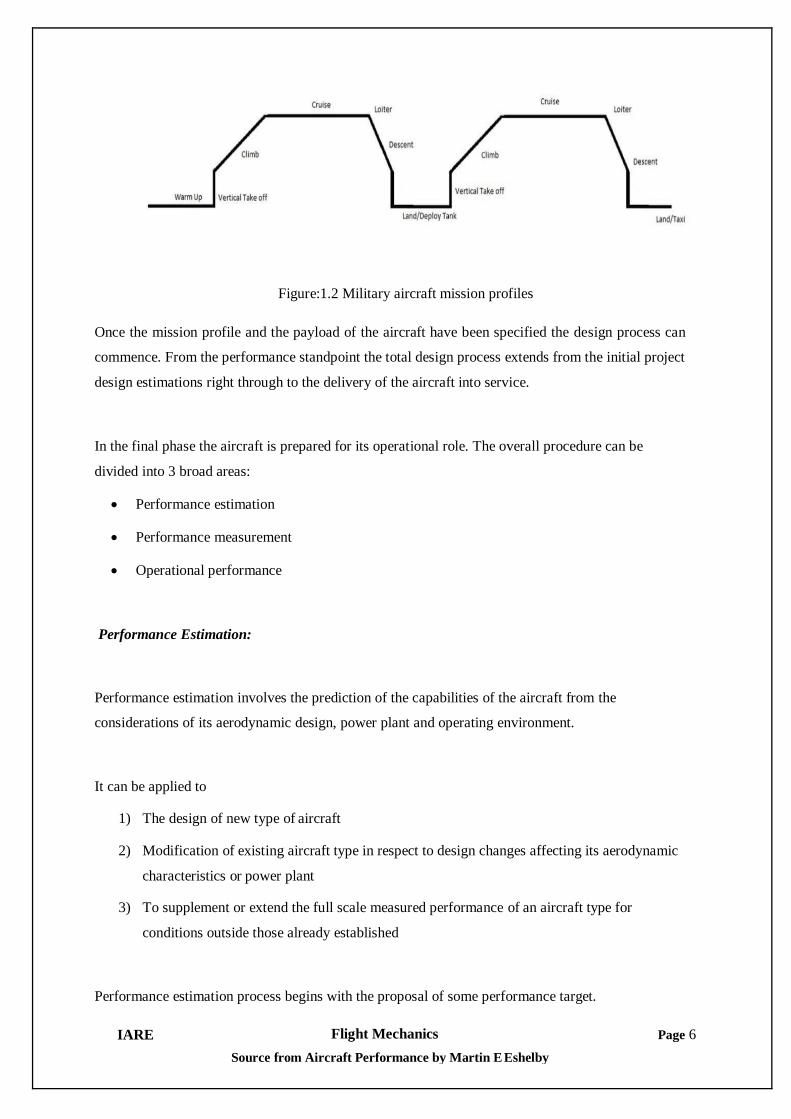


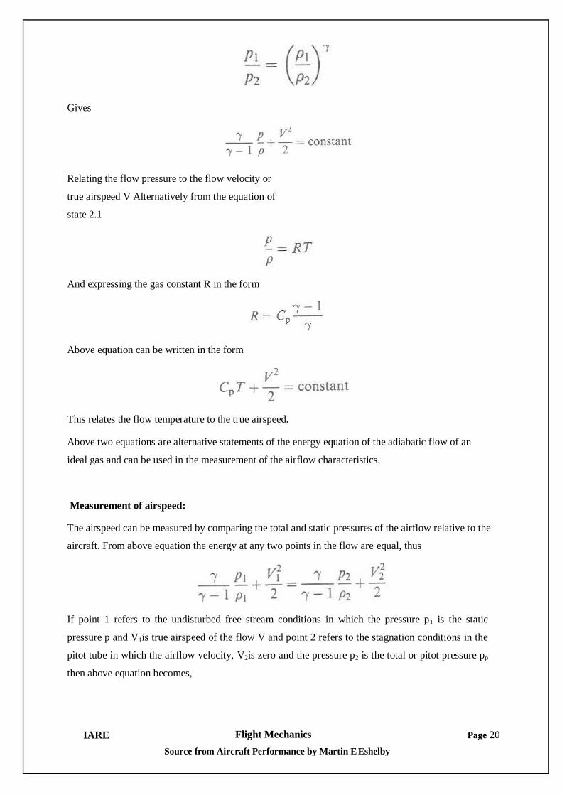


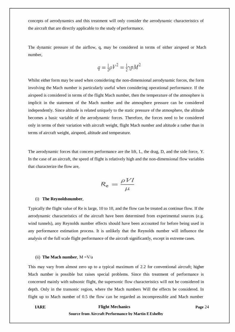


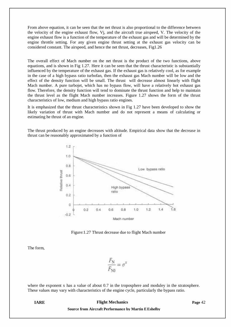

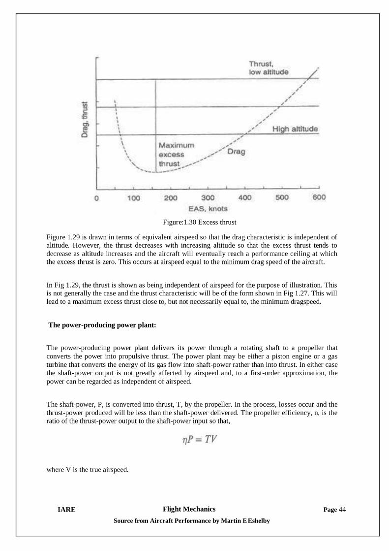

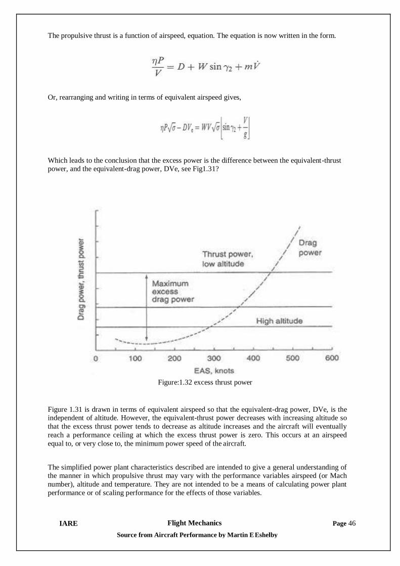
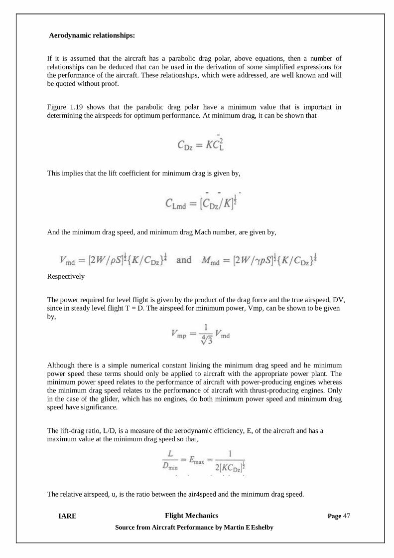


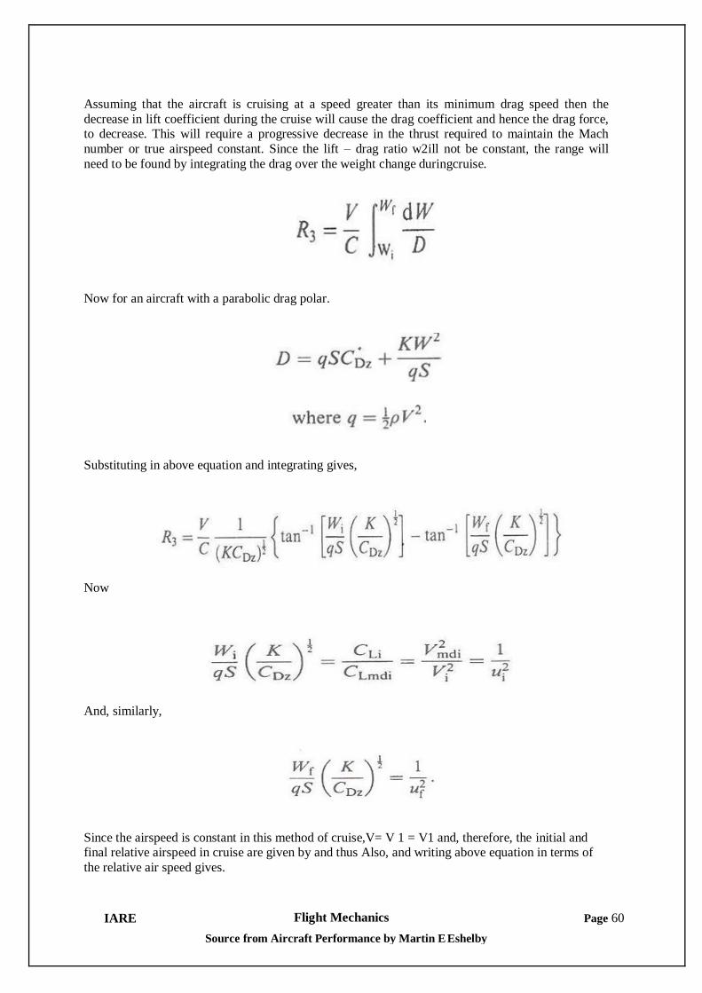


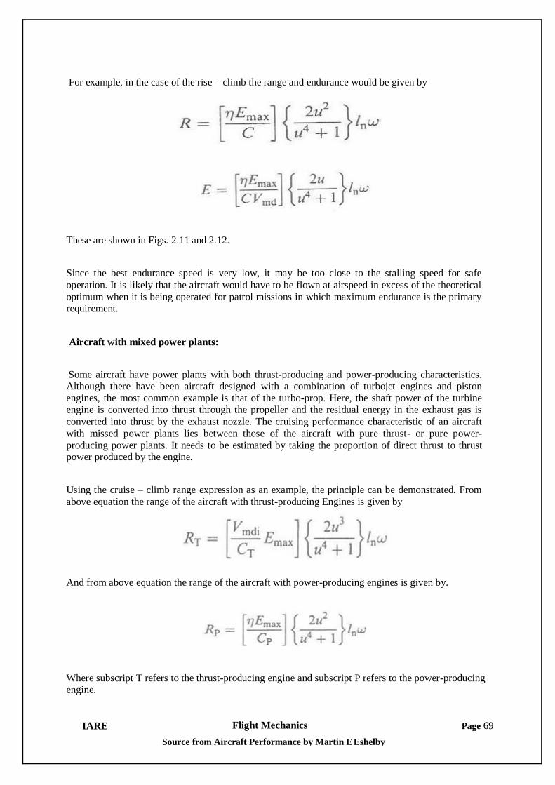


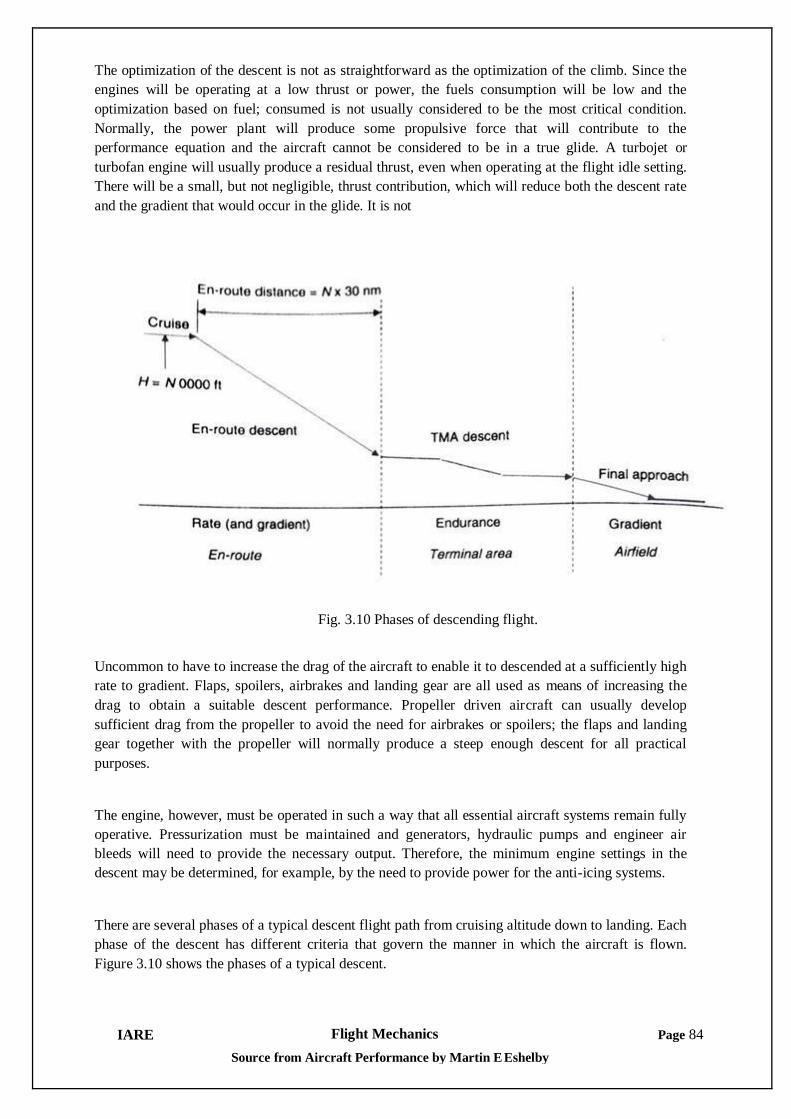


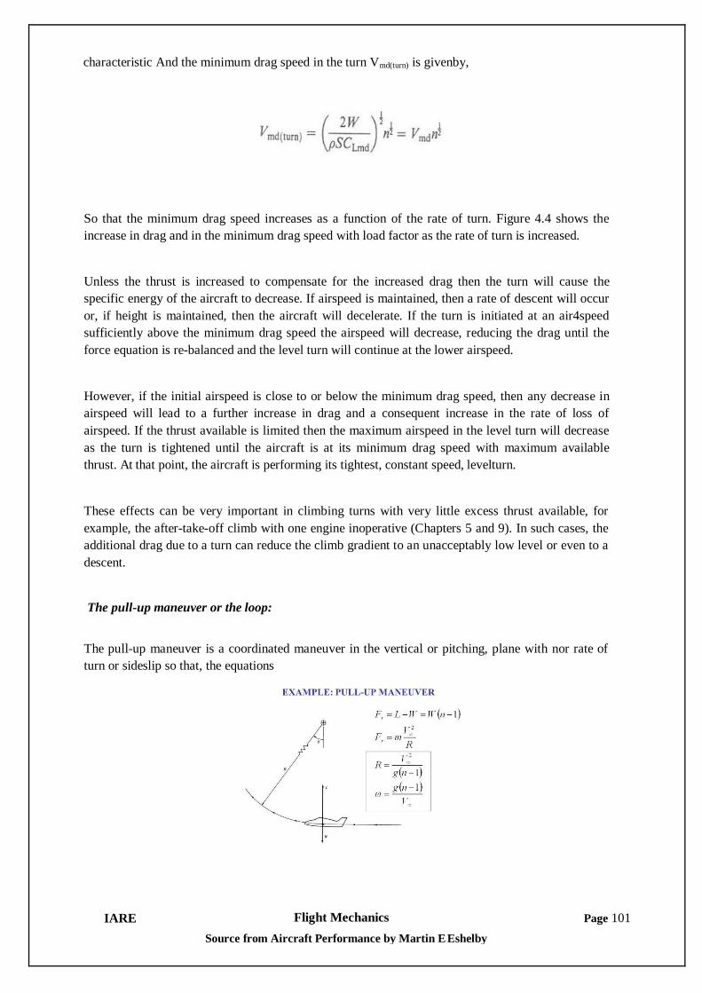

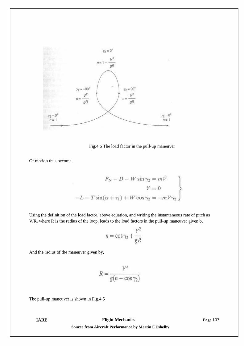


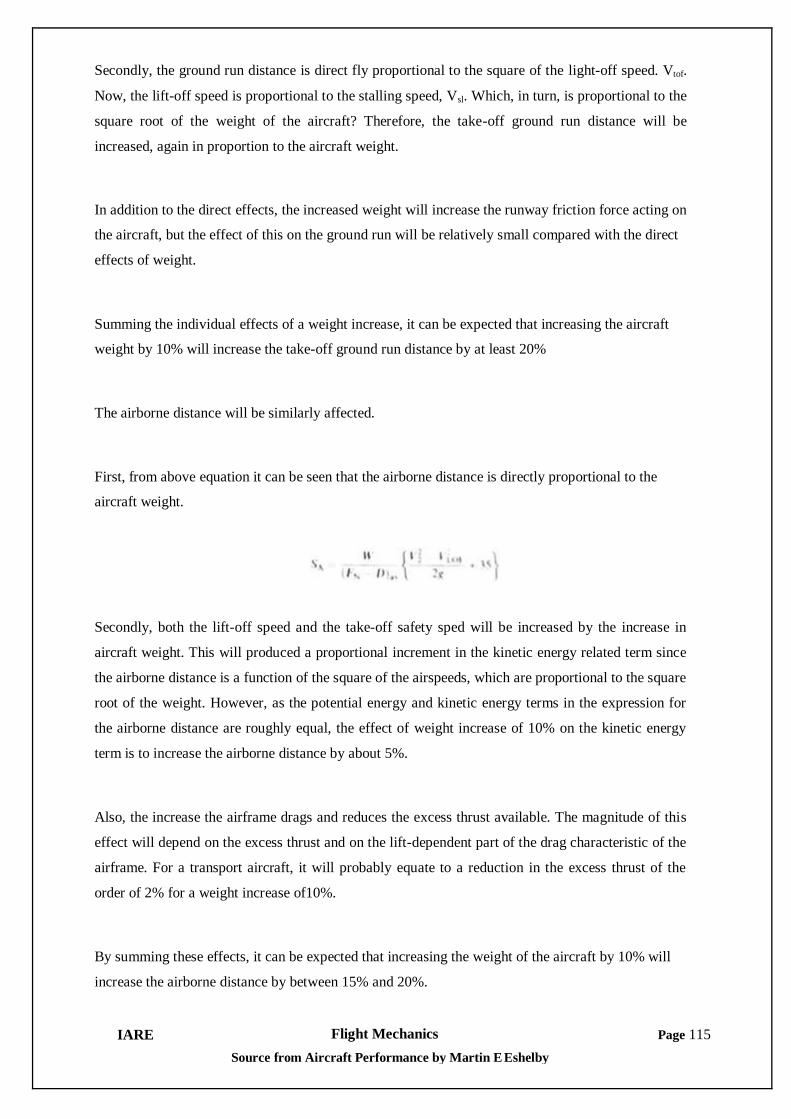


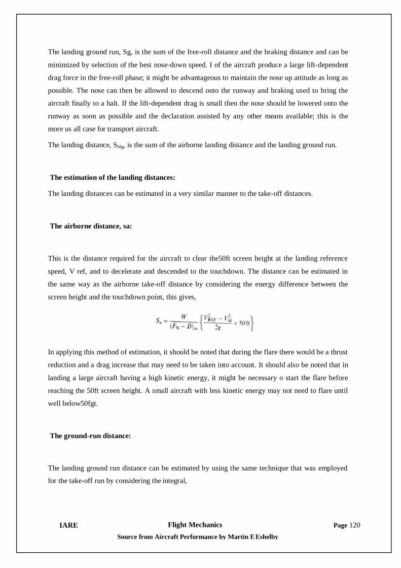


![Aeronautical Development Establishment [ADE] [DRDO institute]](https://static.documents.pub/doc/80x56/553d849b4a79599f2a8b46cb/aeronautical-development-establishment-ade-drdo-institute.jpg)


