Page 1
Instituto Tecnológico y de Estudios Superiores de Monterrey
Campus Monterrey
School of Engineering and Sciences
Characterization of Arc Extinction in Direct Current Residential Circuit
Breakers
A thesis presented by
Julio César Bautista Cruz
Submitted to the
School of Engineering and Sciences
in partial fulfillment of the requirements for the degree of
Master of Science
In
Energy Engineering
Monterrey Nuevo León. May 15th, 2018
Page 3
Instituto Tecnológico y de Estudios Superiores de Monterrey
Campus Monterrey
School of Engineering and Sciences The committee members, hereby, certify that have read the thesis presented by Julio César
Bautista Cruz and that it is fully adequate in scope and quality as a partial requirement for
the degree of Master of Science in Energy Engineering.
Thesis Committee:
____________________________________
Federico Ángel Viramontes Brown, PhD
Tecnológico de Monterrey
Principal Advisor
____________________________________
Carlos Iván Rivera Solorio, PhD
Tecnológico de Monterrey
Committee Member
____________________________________
José Carlos Suarez Guevara, M.SC
Schneider-Electric
Committee Member
____________________________________
Efrain Gutierrez Villanueva, M.SC
Schneider-Electric
Committee Member
_____________________________________
Ruben Morales Melendez, PhD
Dean of Graduate Studies
School of Engineering and Sciences
Monterrey Nuevo León. May 15th, 2018
Page 5
Declaration of Authorship
I, Julio César Bautista Cruz, declare that this thesis titled, “Characterization of Arc
Extinction in Direct Current Residential Circuit Breakers” and the work presented in it are
my own. I confirm that:
This work was done wholly while in candidature for the degree of Master of Science
at this University.
Where I have consulted the published work of others, this is always clearly attributed.
Where I have quoted from the work of others, the source is always given. With the
exception of such quotations, this thesis is entirely my own work.
I have acknowledged all main sources of help.
I have given credence to the contributions of the co-authors.
___________________________
Julio César Bautista Cruz
Monterrey Nuevo León, May 2018
@2018 by Julio César Bautista Cruz
All rights reserved
Page 7
Dedication
To Yahveh my Lord, who has given me the life and has allowed me to consummate my
master's degree, providing me the cleverness, talent, resources and especially wonderful
people who motivated me to move forward.
Page 9
Acknowledgment
To Osvaldo Micheloud and Federico Viramontes for calling me to be part of the Industrial
Consortium to Foster Applied Research in Mexico and for allowing me to join this great
research group.
To my advisor Federico Viramontes, for his support and advice at each stage of the project,
his constant motivation despite all the obstacles encountered and mainly by all the classes
taught by him, always interesting, challenging and with a well-founded purpose.
To Carlos Rivera, for his advice, suggestions, collaboration on this project, and for the
careful revision of the manuscript and useful discussion.
To Efraín Gutiérrez, Mauricio Diaz, José Suarez, José Valerio, of Schneider-Electric, for
supporting me in different means, in addition to the resources for carrying out this research,
review of the manuscript and constant motivation.
To all my professors, since each one of their teaching were vital during the development of
this research.
Page 11
Everything I have accomplished, beyond my effort,
has been the result of my patience.
Julio Bautista
Page 15
Contents
Abstract. ................................................................................................................................... i
Resumen ................................................................................................................................ iii
List of Figures ......................................................................................................................... v
List of Tables ......................................................................................................................... ix
Lexicon .................................................................................................................................. xi
1. CHAPTER I .................................................................................................................... 1
1.1. Introduction .............................................................................................................. 1
1.2. Problem Statement ................................................................................................... 2
1.3. Objectives ................................................................................................................ 2
1.4. Justification .............................................................................................................. 2
1.5. Research questions ................................................................................................... 3
1.6. Scope and Limitations ............................................................................................. 3
1.7. Thesis structure ........................................................................................................ 3
2. CHAPTER II .................................................................................................................. 5
2.1. Characteristics of the electric arc ............................................................................. 5
2.2. Low voltage circuit breakers .................................................................................... 7
Interruption in LVCB ..................................................................................................... 7
2.3. The Limiter Circuit Breaker .................................................................................... 9
2.3.1 Arc breaking .......................................................................................................... 9
2.3.2 Kind of breaking in established currents ............................................................. 10
2.3.3 Arc breaking with limitation................................................................................ 11
2.4. Consequences of Arcing ........................................................................................ 11
2.4.1 Contact Erosion ................................................................................................... 11
2.5. Components of CB ................................................................................................. 12
2.5.1 Frame ................................................................................................................... 12
2.5.2 Contacts ............................................................................................................... 13
2.5.3 Arc Chute Assembly ............................................................................................ 13
2.5.4 Operating Mechanism ......................................................................................... 14
2.5.5 Trip Unit .............................................................................................................. 14
Page 16
2.6. Arc manipulation ................................................................................................... 15
2.6.1. Open Gap ............................................................................................................ 15
2.6.2. Arc Runner ......................................................................................................... 15
2.6.3. Blowout Coils ..................................................................................................... 16
2.6.4. Puffer .................................................................................................................. 16
2.7. Theory of Multi-physical Fields in a Fault Arc ..................................................... 17
2.8. Fluid Models Magnetohydrodynamic description ................................................. 19
2.9. Simulation tool. ...................................................................................................... 20
2.9.1 Ansys-Fluent. ....................................................................................................... 20
2.9.2 ANSYS-Maxwell. ............................................................................................... 21
2.9.3 Altair-Flux ........................................................................................................... 22
3. Chapter III..................................................................................................................... 25
3.1. Methodology for simulation .................................................................................. 25
3.2. Description model .................................................................................................. 27
3.2.1 Geometry model .................................................................................................. 27
3.2.2 Mesh .................................................................................................................... 27
3.2.3 Plasma properties as UDF ................................................................................... 30
3.2.4 Interfaces and boundary conditions ..................................................................... 33
3.2.5 Parametrization .................................................................................................... 35
3.3. Software Set-up ...................................................................................................... 35
3.3.1 Set up in MHD module ........................................................................................ 35
4. Chapter IV .................................................................................................................... 45
4.1. Simulations cases ................................................................................................... 45
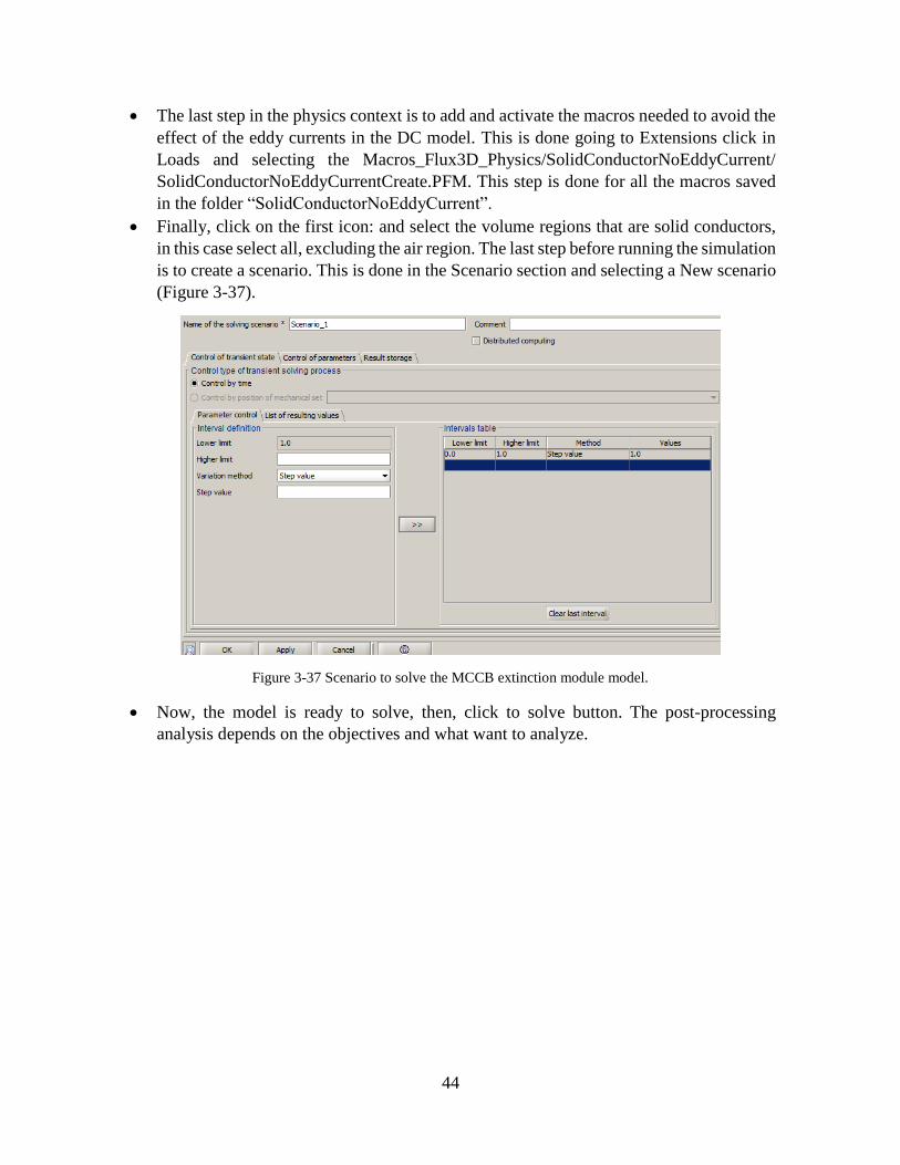
4.2. Case A: Justification analysis ................................................................................ 46
4.3. Case B: Base Model ............................................................................................... 47
4.4. Case C: Coupling Maxwell-Fluent ........................................................................ 47
4.5. Case D: Coupling Flux-Fluent ............................................................................... 48
4.6. Case E: Comparative analysis ................................................................................ 48
5. Chapter V ...................................................................................................................... 49
5.1. Case A1. Justification analysis (3DS model) ......................................................... 49
5.2. Case A2. Justification analysis (3DF model) ......................................................... 51
Comparison case A1 vs case A2 .................................................................................. 52
Page 17
5.3. Case B1. Base Model (laminar regimen) ............................................................... 53
5.4. Case B2. Base Model (turbulent regimen) ............................................................. 60
Comparison case B1 vs case B2 ................................................................................... 67
5.5. Case C1. Coupling Maxwell-Fluent ...................................................................... 68
5.6. Case D1. Coupling Flux-Fluent ............................................................................. 72
Comparison case C1 vs case D2 ................................................................................... 73
5.7. Case E1. Comparative analysis .............................................................................. 74
Comparison case B2 vs case E1 ................................................................................... 79
6. Chapter VI .................................................................................................................... 81
7. Chapter VII ................................................................................................................... 85
Bibliography ......................................................................................................................... 87
A. Appendix A. The Physics of Electric Arc. ................................................................... 91
B. Appendix B. The MHD module of Ansys-Fluent. ....................................................... 93
C. Appendix C. User Define Functions (UDFs) ............................................................... 97
D. Annex D ...................................................................................................................... 101
E. Annex E ...................................................................................................................... 107
Vita ..................................................................................................................................... 109
Page 19
i
Characterization of Arc Extinction in Direct Current Residential Circuit
Breakers
By
Julio César Bautista Cruz
Abstract.
Break the current in a direct current (DC) network is a challenging theme, since the current
does not exhibit a zero crossing point, making it difficult to interrupt. Recent researches show
promising results in the development of Circuit Breakers (CB) for DC, with different
configurations to achieve an artificial zero crossing. However, regardless of the method, the
physical effect of switching is the formation of an electric arc, causing high levels of
temperature, strong magnetic fields, current of several tens of KA, added to mechanical stress
and overpressure on the walls.
Due to this reason, physical phenomena should be studied to determine a suitable design.
This thesis aim is to provide a methodology for the modeling and the comprehension of the
physics that governs electric arc and the role of each component within the CB. To reach this,
the thesis starts by understanding the arc in alternating current (AC), then proceeds to DC. A
theoretical description of the electric arc is outlined, based on plasma physics.
The Magneto-Hydrodynamic (MHD) model is proposed, which allows modeling a plasma
as an electric fluid, allowing coupling the equations of fluid mechanics and magnetic fields.
The scope of the model is the macroscopic scale of the arc dynamics as a conducting,
compressible, viscid fluid, driven by electromagnetic forces and pressure gradients. Some
analysis are performed in different software and a comparative analysis is accomplished.
Finally, the aim of this thesis is to provide to Schneider-Electric Company the background
for this kind of analysis in DC CB.
Page 21
iii
Resumen
Interrumpir el voltaje en una red de corriente directa (DC) es un tema retador, debido a
que la corriente no exhibe un cruce por cero natural, lo que dificulta la interrupción.
Investigaciones recientes muestran resultados prometedores en el desarrollo de Circuit
Breakers (CB) para CD, con diferentes configuraciones para lograr un cruce por cero
artificial. Sin embargo, independientemente del método que se use, el efecto de la
interrupción es la formación de un arco eléctrico, causando incrementos de temperatura,
fuertes campos magnéticos, corrientes de varias decenas de KA, sumado a los esfuerzos
mecánicos provocados por la presión en las paredes.
Por estas razones, estos fenómenos físicos deben estudiarse para determinar un diseño
adecuado. Esta tesis tiene como finalidad proporcionar una metodología para el modelado y
la comprensión de la física que rige el fenómeno de arco eléctrico y el papel de cada
componente dentro del CB. Para llegar a esto, la tesis comienza explicando el fenómeno en
corriente alterna (AC), y luego se procede en CD. Además, se describe la teórica del arco
eléctrico basada en la física del plasma.
Para esto, se propone el modelo Magneto-hidrodinámico (MHD) en ANSYS-Fluent, que
permite modelar un plasma como un fluido eléctrico, permitiendo el acoplamiento de las
ecuaciones de la mecánica de fluidos y los campos magnéticos. El alcance del modelo es un
análisis macroscópico, viendo al arco como un fluido conductor, compresible y viscoso,
impulsado por fuerzas electromagnéticas y gradientes de presión. Algunos análisis se realizan
en diferentes programas y se realiza un análisis comparativo entre ellos. Finalmente, el
objetivo de esta tesis es proporcionar a la compañía Schneider-Electric las bases para este
tipo de estudios en Circuit Brakers de CD.
Page 23
v
List of Figures
Figure 2-1: Cathode fall [16] ............................................................................................................................... 5 Figure 2-2: Anode fall [16] .................................................................................................................................. 6 Figure 2-3 Double break rotary contact, Patent number: 8,159,319 B2. ........................................................... 8 Figure 2-4 the electric arc, composition of the arc column. [28] ........................................................................ 9 Figure 2-5 Arc in extinguishing condition. a- in DC. voltage b- in AC. voltage with Ur of same sign as Ua at the
time of zero current [28]. .................................................................................................................................. 10 Figure 2-6 equivalent circuit in a short circuit fault. ......................................................................................... 10 Figure 2-7 Frame of a Circuit Breaker [31]. ...................................................................................................... 12 Figure 2-8 Straight through contacts and bow apart contacts [30]. ................................................................ 13 Figure 2-9 Arc chute assembly [30]. ................................................................................................................. 14 Figure 2-10 Operating mechanism, a) ON position, b) OFF position [30]. ........................................................ 14 Figure 2-11 Thermal-Magnetic trip unit [30]. ................................................................................................... 15 Figure 2-12 Assembling of arc runners [32]. ..................................................................................................... 16 Figure 2-13 Blowout coils assembling [34]. ...................................................................................................... 16 Figure 2-14 Puffer type SF6 CB, a) ON position, b) OFF position [35]. .............................................................. 17 Figure 2-15 Interaction of physical processes in the arc column [9]. ................................................................ 23 Figure 3-1 Toolbox of Fluent. ............................................................................................................................ 25 Figure 3-2 Geometry with dimensions. ............................................................................................................. 27 Figure 3-3 Overview of the full mesh (a), detailed (b). ..................................................................................... 29 Figure 3-4 Skewness of 3DF mesh. .................................................................................................................... 29 Figure 3-5 Orthogonal quality of 3DF mesh. ..................................................................................................... 29 Figure 3-6 Skewness of 3DS mesh. .................................................................................................................... 30 Figure 3-7 Orthogonal quality of 3DS mesh. ..................................................................................................... 30 Figure 3-8 Density for high temperature air [42], a) plot in TI-Nspire CX CAS software, b) plot in Excel. ........ 31 Figure 3-9 Specific Heat for high temperature air [42], a) plot in TI Nspire CX CAS software, b) plot in Excel. 31 Figure 3-10 Thermal Conductivity for high temperature air [42], a) plot in TI-Nspire CX CAS software, b) plot
in Excel. ............................................................................................................................................................. 31 Figure 3-11 Viscosity for high temperature air [42], a) plot in TI-Nspire CX CAS software, b) plot in Excel. .... 32 Figure 3-12 Electric Conductivity for high temperature air [42], a) plot in TI-Nspire CX CAS software, b) plot in
Excel. ................................................................................................................................................................. 32 Figure 3-13 Boundary conditions on the model. ............................................................................................... 34 Figure 3-14 Modules of ANSYS Fluent. ............................................................................................................. 36 Figure 3-15 Set-up MHD module. ..................................................................................................................... 36 Figure 3-16 Set-up of transient simulation, P1 radiation model and turbulent analysis. ................................. 37 Figure 3-17 Compilation of plasma properties. ................................................................................................ 37 Figure 3-18 Loading material properties. ......................................................................................................... 37 Figure 3-19 Set-up cell zone condition. ............................................................................................................. 37 Figure 3-20 Configuration of limits of the simulation. ...................................................................................... 38 Figure 3-21 Advance configurations for the solution controls. ......................................................................... 38 Figure 3-22 Solution Methods Set-up Fluent. ................................................................................................... 38 Figure 3-23 Solution Controls Set-up Fluent. .................................................................................................... 38 Figure 3-24 Set-up of Run Calculation. ............................................................................................................. 39 Figure 3-25 Toolbox of Maxwell. ...................................................................................................................... 39 Figure 3-26 Assignation of each zone in the geometry .................................................................................... 39 Figure 3-27 Set-up of Magnetostatic simulation and assign of direction current in Maxwell. ......................... 40
Page 24
vi
Figure 3-28 Set-up Mesh length in Maxwell. .................................................................................................... 40 Figure 3-29 Configuration of Fluent conductivity coupling............................................................................... 41 Figure 3-30 Validation check of the set-up. ...................................................................................................... 41 Figure 3-31 Geometry imported from the modeler context. ............................................................................ 41 Figure 3-32 Mesh model of the CB. .................................................................................................................. 42 Figure 3-33 Configuration of the formulation model in Transient Magnetic 3D application. .......................... 42 Figure 3-34 Current applied to the model in the circuit dedicated context. ..................................................... 42 Figure 3-35 Importing material from material manager. ................................................................................. 43 Figure 3-36 Assignment terminals to solid conductors. .................................................................................... 43 Figure 3-37 Scenario to solve the MCCB extinction module model. ................................................................. 44 Figure 5-1 Arc movement, expressed by temperature for case A1. .................................................................. 50 Figure 5-2 Maximum temperature in air for case A1. ...................................................................................... 50 Figure 5-3 Arc movement, expressed by temperature for case A2. .................................................................. 51 Figure 5-4 Maximum temperature in air for case A2. ...................................................................................... 52 Figure 5-5 Arc movement, expressed by temperature and current density for case B1. .................................. 53 Figure 5-6 Maximum electric potential for case B1. ......................................................................................... 54 Figure 5-7 Maximum temperature in air for case B1. ...................................................................................... 55 Figure 5-8 Maximum temperature in Anode and Cathode for case B1. ........................................................... 56 Figure 5-9 Maximum temperature in splitter for case B1. ............................................................................... 56 Figure 5-10 Maximum radiation temperature for walls for case B1. ............................................................... 57 Figure 5-11 Maximum current density in air for case B1. ................................................................................. 58 Figure 5-12 Maximum current density at the splitter for case B1. ................................................................... 58 Figure 5-13 Maximum absolute pressure for case B1. ..................................................................................... 59 Figure 5-14 Arc movement, expressed by temperature and current density for case B2. ................................ 61 Figure 5-15 Maximum electric potential for case B2. ....................................................................................... 62 Figure 5-16 Maximum temperature in air for case B2. .................................................................................... 63 Figure 5-17 Maximum temperature in Anode and Cathode for case B2. ......................................................... 63 Figure 5-18 Maximum temperature in splitter for case B2. ............................................................................. 64 Figure 5-19 Maximum radiation temperature for walls for case B2. ............................................................... 64 Figure 5-20 Maximum current density in the air for case B2. .......................................................................... 65 Figure 5-21 Maximum current density at the splitter for case B2. ................................................................... 66 Figure 5-22 Maximum absolute pressure for case B2. ..................................................................................... 66 Figure 5-23 Arc movement, expressed by temperature (left) and current density (right) for case C1. ............ 68 Figure 5-24 Maximum temperature in Air for case C1. .................................................................................... 69 Figure 5-25 Arc movement, expressed by Magnetic Flux Density for case C1. ................................................. 70 Figure 5-26 Maximum magnetic flux density for case C1. ................................................................................ 71 Figure 5-27 Arc movement, expressed by geometry for case D1. .................................................................... 72 Figure 5-28 Maximum magnetic flux density for case D1. ............................................................................... 73 Figure 5-29 Arc movement, expressed by temperature and current density for case E1. ................................ 74 Figure 5-30 Maximum temperature in Air for case E1. .................................................................................... 75 Figure 5-31 Maximum temperature in Anode and Cathode for case E1. ......................................................... 76 Figure 5-32 Maximum current density in the air for case E1. ........................................................................... 76 Figure 5-33 Maximum current density at the splitter for case E1. ................................................................... 77 Figure 5-34 Maximum electric potential for case E1. ....................................................................................... 77 Figure 5-35 Maximum radiation temperature for walls for case E1. ............................................................... 78 Figure 5-36 Maximum absolute pressure for case E1. ...................................................................................... 79 Figure A-1 Electron trajectory in a homogeneous electric field. The trajectory is interrupted by elastic
collisions with neutral atoms.[45] .................................................................................................................... 92 Figure B-1 Modules of ANSYS Fluent. ............................................................................................................... 95
Page 25
vii
Figure C-1 Grid components [41]. ..................................................................................................................... 98 Figure C-2 Example of UDF codification. .......................................................................................................... 99 Figure D-1 Arc movement images from reference [9]. ................................................................................... 101 Figure D-2 Arc movement, (temperature and current density) for case B1. ................................................... 102 Figure D-3 Arc movement, (temperature and current density) for case B2. ................................................... 103 Figure D-4 Arc movement, (temperature and current density) for case C1. ................................................... 104 Figure D-5 Arc movement, (temperature and current density) for case E1. ................................................... 105
Page 27
ix
List of Tables
Table 2-1 Minimum voltage and current in different materials ......................................................................... 6 Table 3-1 Description of the 3DF mesh ............................................................................................................. 28 Table 3-2 Description of the 3DS mesh. ............................................................................................................ 28 Table 3-3 Boundary conditions applied in the model ....................................................................................... 33 Table 4-1 Cases analyzed .................................................................................................................................. 45 Table B-1 User-Define Scalars in MHD Model .................................................................................................. 95 Table C-1 Grid nomenclature. ........................................................................................................................... 98
Page 29
xi
Lexicon
2D. Bi-dimensional
3D. Tri-dimensional
3DF. Tridimensional analysis full
3DS. Tridimensional analysis simplified
AC. Alternating current
Arc chute. Series of plates in the path of that arc that split it up into smaller segments
Arc column. Region where the ions and electrons circulate through a column of ionized
gases and metallic vapors, this zone is considered as quasi-neutral fluid.
Arc root. Short segment of the electric arc, where the arc surges from the cathode or the
anode.
B. Magnetic flux density
CB. Circuit Breaker
CFD. Computerized Fluid Dynamics.
Contact. Static or dynamic elements, which allow current to flow between them.
DC. Direct current
Drift velocity. Average velocity that a particle, such as an electron, attains in a material due
Electric arc
HVCB. High Voltage Circuit Breaker.
Ionization. Process by which an atom or a molecule acquires a negative or positive charge
by gaining or losing electrons to form ions.
J. Current density
Lorentz force. Combination of electric and magnetic force on a point charge due to
electromagnetic fields.
LTE. Local Thermic Equilibrium.
LVCB. Low Voltage Circuit Breaker.
MCCB. Molded Case Circuit Breaker.
MVCB. Medium Voltage Circuit Breaker
P. Pressure
Plasma. Fourth state of the matter, created by the ionization of a gas.
T. Temperature
Terminals. Extreme of the current path in the circuit breaker.
Trip unit. Module of a circuit breaker that sends a signal to interrupt the current through
the circuit.
Page 31
1
1. CHAPTER I
1.1. Introduction
At present, it is well known that the growth in the generation of electric power systems,
the emergence of renewable sources and the need for reliable power distribution systems
have caused to reconsider the use of direct current (DC) instead of alternating current (AC).
This new approach is taken because of the different benefits of the DC distribution and
interconnection with renewable energy sources, control systems, train systems and
construction industry, to name a few.
On the other hand, DC-based systems are defenseless against faults in the transmission
and distribution lines, which can lead to the destruction of electronic devices instantly [1],
[2]. For this reason, it is necessary to detect faults in the network to achieve a quick
interruption of high levels of currents. To make the rapid detection and interruption of
current, devices known as Circuit Breakers (CB) are used, which can detect overcurrent
levels and open immediately to stop the current.
However, achieving this interruption in a DC line can be complicated, since the key to
carry through this is an absent primordial element, which is zero crossing point. Given that
this element does not exist in DC, procedures to force this artificially cross must be
implemented. Fortunately for voltages at residential levels (120V in AC), the CB just must
generate and maintain an arc voltage which in turn causes the arc to collapse and interrupt
the current.
In the case of voltages over the residential level, there are several papers referred to
DCCB, which have developed different methods to switch current, some are: current
injection in reverse through parallel capacitor [3]; Ballistic CB with resistors in series to
distribute the arc [4]; mechanical contacts with high speed actuators [5]; interruption of arc
by transverse or axial magnetic fields [6], [7]; use of inductors for automatic detection of arcs
[8], to mention a few of the most recent methods used.
Regardless of the method, the physical effect of switching is the formation of an electric
arc within the CB, causing high levels of temperature, strong magnetic fields, current of
several tens of KA, added to mechanical stress and overpressure on the walls. Due to these
reasons, physical phenomena should be studied to determine a suitable design.
For the purpose of this project, the electric arc will be modeling through a Computational
Fluid Dynamics (CFD) software, coupling the Maxwell equations for electromagnetic fields
and the Navier Stokes equations. For this coupling, the software of ANSYS (Fluent,
Maxwell) and ALTAIR-FLUX will be used. Important research about arc modeling have
been studying in [9], [10], [11], where the simulation processes are explained in great detail,
exposing results such as voltages, currents, pressures and temperatures. In the case of [9]
experimental tests are also carried out.
Page 32
2
1.2. Problem Statement
Currently there is a lot of information related to modeling the electric arc, however,
nowhere is the simulation process that need to be followed for the correct characterization.
For this reason, it is necessary to give an answer and propose the methodology to follow for
the correct simulation related to the interruption of a DC short circuit fault, detailing the steps
and the initial and boundary conditions in the model. The simulation must include the levels
due to temperatures and pressures in the CB.
1.3. Objectives
The main objective here involves the simulation of the thermal and magnetic phenomena
produced by the interruption process during a short circuit fault in a DC CB.
Particularly objectives are intended to cover the following points:
Development of a suitable methodology to characterize the electric arc using the MHD
module of Fluent.
Perform a coupling between Maxwell-Fluent and Flux-Fluent to obtain the magnetic
flux density (B).
Determine the maximum values of temperature and overpressure reached within the
CB. Conduct a comparison of results with [9].
Use the MHD methodology in a static model (no electrodes movement) using a
simplified CB geometry.
The thesis mentioned in reference [9] has been chosen as a comparison, since it offers a
geometry easy to analyze, the methodology and boundary conditions are presented in detail,
as well as offering simulation results together with experimental tests.
1.4. Justification
It is necessary to know the physics that governs the electric arc phenomenon. Also, it is
expected to know the interaction of the components and meet the performance of the CB
during an arc extinction, which requires the application of specialized software that allows
characterizing such phenomena.
This thesis proposal is made to develop a project raised by Schneider Electric Company,
which previously has been tested successfully for adaptations of CB from AC to DC at
medium voltage level (Compact NSX DC & DC PV model), however, now the purpose is in
residential level (low voltage). Considering that nowadays they have a functional design of
an AC CB (QO model), this is a standard thermal-magnetic to 15 and 20 amperes CB, which
can provide overload and short-circuit protection for conductors [12].
It is expected that the results of this thesis can help to understand the electric arc
phenomenon and the improvement of a DC CB at residential level.
Page 33
3
1.5. Research questions
1. What is an electric arc and what are the physical properties that it presents (electrical
conductivity, viscosity, density, etc.)?
2. What is a Breaker, features and components?
3. What are the consequences of arc extinction within a Breaker?
4. What are the main factors that intervene during the formation of an electric
(temperatures, current levels) arc and how an electric arc can be modeled?
1.6. Scope and Limitations
The scope of this investigation begins by understanding the physical phenomena in CB
for AC (bibliographic research), then proceed in DC, this includes equations that govern the
electric arc, modeling of the magnetic forces, arc power, thermal energy and fluid flow. Once
these points were covered, the simulation of a static CB is done (2D and 3D). Verifying its
correct performance, through comparisons with the results from [9].
Some of the most critical limitations of the project are, the LVCB is the most difficult to
simulate [13], because current is difficult to maintain during simulations. Here, further
phenomena such as arc motion along rail electrodes, arc birth, eddy currents, and the
interaction between the arc and the external circuit have not been considered (as a
simplification). In addition, all effects are strongly coupled and cannot be validated
separately, unfortunately, there is not good arc simulation tool available on the market.
Industrial researchers typically couple different tools, Fluent + electromagnetic solver, for
example: Fluent + MpCCI + ANSYS EMAG [14]. Therefore, the biggest limiting will be
achieving a good coupling of the different tools for modeling the arc.
1.7. Thesis structure
This thesis is divided into 7 chapters. Chapter 1 describes the justification, objectives,
and scope of the project. Chapter 2 deals with the characteristics of the electric arc,
consequences of interruption, explanation of CBs, as well as their operation. Subsequent to
this, the theory for the modeling of the electric arc is also described, as well as the necessary
simplifications.
In Chapter 3, the methodology for the simulation is explained. The model to be used is
defined, such as geometry, mesh, and boundary conditions. Also, the setup is explicated for
each of the software used. In chapter 4 all the cases to be analyzed are described, where the
modifications of each one are exposed and what is expected to be obtained. After that, in
chapter 5 the results of the simulations are presented, the results are described in addition to
the variations with respect to each case. Here the results are presented in terms of graphs and
contours.
In chapter 6 the conclusions of this thesis are presented, starting with a summary of
chapter 1-4 and later highlighting the most important results of chapter 5. Finally, in chapter
7 the future works are presented based on what was developed in this thesis.
Page 35
5
2. CHAPTER II
2.1. Characteristics of the electric arc
The internal arc fault is a very severe short-circuit fault that can occur in electrical
equipment [15]. In a conventional way, the current flows in a solid conductor; when an arc
fault occurs, this current flows through the air between two conductors (anode-cathode).
In one side the cathode contact provides the electrons to allow the arc to continue between
the contacts (Figure 2-1). The cathode region can be described with a high electric field of
108-109 volts/meter. In general, the electron emission involves a combination of thermally
enhanced field emission (T-F emission) and the effects of ion bombardment. In the cathode
fall region, about 90% of the current is carried by electron and 10% is carried by ions. The
voltage drop in the cathode fall is approximately 15 volts. Cathode temperature is
comparable the boiling point of contact material. The high electron emission is produced by
heat and enhanced field emission. The current density of the spot is about 103-106 A/cm2
[16].
Figure 2-1: Cathode fall [16]
The arc column has the characteristics of a plasma. The density of the electrons and ions
are equal. In addition, the temperature of the electron and ions are equal to the gas
temperature [16].
On the other hand, the anode region serves to collects the electrons carrying the current
from the arc column (Figure 2-2). The thermal boundary layer between the arc column and
the anode surface is small. The electron density gradients are high so that electron diffusion
flow exists. The anode fall voltages can be close to zero and as high as 15-20 volts. The anode
fall temperature is about 200-degrees C up to the boiling point of the contact material. The
current is carried by electrons and anode spot current density is less than that of the cathode
spot.
Page 36
6
Figure 2-2: Anode fall [16]
When a fault is detected in an AC network, the CB starts to open to break the current,
during this process an electric arc is built between opening contacts, which must be
maintained to achieve a successful current interruption.
Nevertheless, many conditions are necessary to attain this. Thus, the arc is ignited. The
arc cannot exist if the arc current is lower than the minimum arc current. The value of this is
a characteristic of the contact material, [16]. When the arc starts, the arc voltage must have a
minimum value, this can be determined by the current magnitude, the gap width, and the
orientations of electrodes [17].
An already established arc requires a continuous flow of electrons from the cathode to be
sustained. Below some minimum value 𝐼𝐴 ≤ 𝐼𝑚𝑖𝑛, the energy losses will exceed the
introduced energy to the cathode and the arc will be extinguished.
A minimum voltage, Umin, is also required across the open contacts to sustain the arc. The
electric arc would at least require a voltage that corresponds to the ionization potential of the
gas, Vi, and the work function voltage, Uϕ, of the cathode contact. It is, therefore, reasonable
to assume that [18]:
𝑈𝑚𝑖𝑛 ≈ 𝑉𝑖 + 𝑈𝜙
Calculated values for Vi + Uϕ is compared to measured value for Umin and Imin for different
contact materials in Table 2-1.
Table 2-1 Minimum voltage and current in different materials
𝑉𝑖 𝑉𝜙 𝑉𝑖 + 𝑉𝜙 𝑉𝑚𝑖𝑛 𝐼𝑚𝑖𝑛 (volts) (volts) (volts) (volts) (Amperes)
Al 5.98 4.10 10.08 11.2 0.4
Ag 7.57 4.74 12.31 12 0.4
Cu 7.72 4.72 12.19 13 0.4
Fe 7.90 4.63 12.53 12.5 0.45
Page 37
7
During a circuit fault, the CB is turned off or is tripped, this interrupts the flow of current
by separating its contacts. The current through the conductors of the CB generates a magnetic
field in the arc chamber.
The electromagnetic and thermal forces of the arc are supplemented to force the arc away
from the contact region along arc runners and directly into the arc chutes. This assembly is
made up of several “U” shaped steel plates that surround the contacts. As the arc develops, it
is drawn into the arc chute where it is divided into smaller arcs, which are extinguished faster.
Minimizing the arc is important for two reasons. First, arcing can damage the contacts.
Second, the arc ionizes gases inside the molded case [15].
In turn, the current is reduced. Therefore, the arc cannot be maintained. The resistance of
the arc and the arc voltage can be varied by increasing the length of the arc, cooling the arc
and splitting the arc into a number of series arcs [16]. For more information about the arc
physics, consult annex A.
2.2. Low voltage circuit breakers
A circuit breaker is a device designed not only to protect the load and cables but also for
safety and security of the human life. All circuit breakers protect the circuit conductors
mainly by detecting and interrupting the overcurrent [19]–[23].
The opening of the circuit breaker is a reaction to situations of transient current, such as
short circuits or faults in the electrical system. The circuit breakers are classified according
to the available interruption capacity and the nominal direct current (Low-voltage circuit
breakers, Molded Case Circuit Breakers, (MCCB), Low Voltage Power Circuit Breakers
(LVPCB), Isolated Circuit Breakers (ICCB), Mini Circuit Breakers (MCB) to mention a few)
[24].
The interrupting capacity of a circuit breaker is the maximum short-circuit current that the
circuit breaker can safely interrupt at a defined voltage. This short-circuit current described
by current magnitude and its value is in symmetrical amperes rms. The amount of current
that a circuit breaker can transmit until it reaches the overload conditions and opens the circuit
is defined as the DC classification [25], [26],[27].
Interruption in LVCB
At low voltage, the LVCBs are the most important devices for the extinction of electric
arc. Most of them are very similar in layout design and structure, even though some
differences exist. This way, the general layout of a conventional LVCB can be seen in Figure
2-3, including the following components:
Page 38
8
Figure 2-3 Double break rotary contact, Patent number: 8,159,319 B2.
Upper connection: To connect the circuit breaker with the electrical circuit.
Fixed and movable contacts: where the electric arc is formed when these contacts
separate physically.
Arc chamber and splitter plates stack: it is constituted by several plates, arranged in
parallel between them. The aim is to split the arc into smaller arcs, in order to lengthen
and extinguish it. In some references, the arc chamber is also known as arc chute.
Talking about conventional CB, generally use air for current interruption, with little
differences in details and components, the general construction is showed in Figure 2-3,
includes: the main contacts designed to carry the current under normal operating conditions,
the arcing contacts (also called rails) the arc chamber, enclosure and the trip unit. In many
cases, the geometry of the current carrying parts produces a magnetic force that moves the
arc into the chamber. This way, some designs use coils for increasing the magnetic force,
while others help the arc by blowing air [9].
The typical sequence in a LV conventional air circuit breaker is the following:
The main contacts open while the arc contacts remain closed.
The arcing contacts open and the arc starts to move along their length.
The magnetic force produced by the arc current or by blowing coils moves the arc to
the arc chamber.
The arc is divided into several small arcs in series, by the plates of the arc chamber.
he arc chamber allows cooling the arc, lengthening and narrowing its section until
the current is interrupted.
The arc chamber enables the ionization products to be dissipated or absorbed,
restoring the dielectric strength in the air space between the contacts.
The conventional LVCBs described establish the arc in the interrupting medium, air in most
LV switches, and maintain it until the next natural zero current for AC cases or until the
voltage drop of the arc rises above circuit’s voltage for DC cases. Then, the arc is
extinguished [9].
Page 39
9
2.3. The Limiter Circuit Breaker
As was mentioned below, to achieve a successful interruption, a CB must generate an arc
voltage which in turn causes the arc to collapse. This kind of CB is known as Limiting
Circuit-Breaker. A current limitation is achieved by making use of the arc voltage under fault
conditions. This arc must be well managed, that is to say:
The arc voltage must be sufficient value to facilitate high limitation and rapid
extinction,
Dielectric regeneration properties when the arc current reaches zero.
Further, the limiting CB must exhibit several properties under high short-circuit currents:
A minimum current to ensure contact repulsion
A transitive energy value,
A short arc voltage duration,
A maximum value of arc voltage, which is independent of the fault current.
The model also must take into account the external parameters of electric network being
considered: voltage, frequency, short-circuit level, number of phases, etc. [28].
2.3.1 Arc breaking
The arc corresponds to a 4th physical condition: plasma. As soon as two contacts separate,
one of them (cathode) transmits electrons and the other one (anode) receives them, and since
electronic emission is by its very nature energy generating, the cathode will be hot (Figure
2-4). Resulting in arc stagnation which can give rise to metallic vapors. These vapors and the
ambient gas will then be ionized, hence [28]:
more free electrons;
creation of positive ions which drop back on the cathode, thus maintaining its high
temperature;
creation of negative ions which bombard the anode causing temperature to rise.
Figure 2-4 the electric arc, composition of the arc column. [28]
Page 40
10
This natural phenomenon, once controlled, proved to be an irreplaceable intermediary for
current breaking. Breaking control must relate to at least two specific arc-related aspects:
Arc voltage helps reduce current strength and,
Arc extinguishing conditions when the current moves to zero are met if dielectric
regeneration is quickly achieved.
This regeneration must take place despite the presence of mains voltage and of the
overvoltage phenomenon due to the circuit stray capacity (transient recovery voltage or
TRV). The Figure 2-5 shows the TRV on breaking of DC and AC current. Consult annex A
for more details about the arc physics.
2.3.2 Kind of breaking in established currents
In both cases considered below (AC or DC), the current is in steady state before breaking.
In a DC voltage
As soon as the contacts open, an arc voltage appears and the current will start to decrease.
The equation governing the circuit becomes:
𝑈𝑟(𝑡) − 𝑅𝑖 − 𝐿𝑑𝑖
𝑑𝑡− 𝑈𝑎(𝑡) = 0 Ec. 2-1
Figure 2-6 equivalent circuit in a short circuit fault.
Figure 2-5 Arc in extinguishing condition. a- in DC. voltage b- in AC. voltage with Ur of same sign as Ua
at the time of zero current [28].
a b
Ur recovery voltage
Ud regeneration characteristics
i current at an instant t
u voltage at an instant t
Page 41
11
It appears that current i cannot be forced to 0 unless arc voltage Ua becomes and remains
greater than mains voltage E. Since the arc voltage is greater than mains voltage when the
current is canceled, the resulting dielectric regeneration is problem free. Figure 2-6 shows an
equivalent short-circuit fault.
In an AC voltage
In this case, the steady state current passes regularly via the zero value. The first condition
to be reached is thus the quick dielectric regeneration of the arc when the current passes to
zero, despite the presence of the mains voltage. Successful breaking is in practice a
competition of speed between dielectric regeneration and evolution of mains voltage.
2.3.3 Arc breaking with limitation
“With limitation” means that measures are taken to prevent the short-circuit current having
the time to reach its maximum value, (about 63% of maximum fault current).
This current limitation will be obtained if arc voltage Ua quickly becomes greater than
mains voltage and remains so until the current is canceled. In point of fact, the generalized
Ohm´s law, (n is the number of splitters in the arc chamber and Ua is around 25-30 V [18]:
𝑈𝑟 − 𝑅𝑖 − 𝐿𝑑𝑖
𝑑𝑡− 𝑛 ∙ 𝑈𝑎(𝑡) = 0 Ec. 2-2
The Ec. 2-2 shows that di/dt will change sign as soon as Ua (t)>Ur (t) both in DC and AC
voltage. Limitation devices are based on current effects beyond a certain threshold, the short-
circuit current creates thermal effects (fuse) or electromagnetic effects (circuit breakers) and
generates an arc voltage [29].
2.4. Consequences of Arcing
The presence of an electric arc has both positive and negative consequences. The positive
aspect is that the arc allows for a smooth decrease to zero current. If the circuit current were
to suddenly drop to zero at the moment of contact separation, the energy stored in the
inductance, L, would cause an over-voltage given by [18]:
𝑉 = −𝐿𝑑𝐼
𝑑𝑡 Ec. 2-3
The presence of an electric arc usually limits the over-voltage to a maximum of two or
three times the circuit voltage. Without this feature, switch designers would have to design
to protect the circuit against large over-voltages.
However, other consequences of arcing could be devastating for the switching device and
affect the design and choice of materials.
2.4.1 Contact Erosion
Since erosion of the contact material is one of the most important consequences of arcing
and the design is directly relating to the lifetime of the device. It occurs because both the
anode and cathode heats up to above the boiling temperature of the contact material. The
Page 42
12
temperature of the arc is so high that erosion occurs even if the arc is moving across the
contact surfaces. The amount of erosion depends on many parameters, for example:
Circuit current
Arcing time
Open gap distance
Contact material
Size and shape of the contact
Contact opening velocity
Arc motion on the contacts
Design of the arc chamber
2.5. Components of CB
Many of the principals used by circuit breaker engineers to analyze and design DC circuit
breakers to interrupt DC currents are carried over from AC devices. The physics of open gap,
arc runners, slot motors, reverse loops, and arc chutes also apply in DC systems. One might
say that the use of these design strategies is even more demanding in DC circuit breakers due
to the added burden of quenching the arc without the aid of a current crossing zero. The basic
of circuit breaker design and construction, are created from the following five major
components, Frame, Contacts, Arc Chute Assembly, Operating Mechanism and Trip Unit
[1].
2.5.1 Frame
The frame provides an insulated housing to mount the circuit breaker components (Figure
2-7). The construction material is usually a thermal set plastic, such as glass-polymer. The
construction material can be a factor in determining the interruption rating of the circuit
breaker. Typical frame ratings include, maximum voltage, maximum ampere rating, and
interrupting rating [30].
Figure 2-7 Frame of a Circuit Breaker [31].
Page 43
13
2.5.2 Contacts
The current flowing in a circuit controlled by a circuit breaker flows through the circuit
breaker’s contacts. When a circuit breaker is turned off or is tripped by a fault current, the
circuit breaker interrupts the flow of current by separating its contacts.
Contacts are of two types depending on the interrupting rating: Straight-Through Contacts
and Blow-Apart Contacts [30].
a) b)
Figure 2-8 Straight through contacts and bow apart contacts [30].
Straight-Through Contacts
Some circuit breakers use a straight-through contact arrangement, so called because
the current flowing in one contact arm continues in a straight line through the other
contact arm (Figure 2-8 a).
Blow-Apart Contacts
With this design, the two contact arms are positioned parallel to each other. As current
flows through the contact arms, magnetic fields develop around each arm. Because
the current flow in one arm is opposite in direction to the current flow in the other,
the two magnetic fields oppose each other. Under normal conditions, the magnetic
fields are not strong enough to force the contacts apart. When a fault develops, current
increases rapidly causing the strength of the magnetic fields surrounding the contacts
to increase as well (Figure 2-8 b).
2.5.3 Arc Chute Assembly
The arc is extinguished in this assembly. When a circuit breaker is turned off or is tripped
by a fault current, the circuit breaker interrupts the flow of current by separating its contacts.
This assembly is made up of several “U” shaped steel plates that surround the contacts
(Figure 2-9). As the arc develops, it is drawn into the arc chute where it is divided into smaller
arcs, which are extinguished faster [30].
Page 44
14
Figure 2-9 Arc chute assembly [30].
Minimizing the arc is important for two reasons. 1) Arcing can damage the contacts, 2)
the arc ionizes gases inside the molded case. If the arc isn’t extinguished quickly the pressure
from the ionized gases can cause the molded case to rupture.
2.5.4 Operating Mechanism
The operating handle is connected to the moveable contact arm through an operating
mechanism. In the following illustration, the operating handle is moved from the “OFF” to
the “ON” position Figure 2-10. In this process, a spring begins to apply tension to the
mechanism. When the handle is directly over the center, the tension in the spring is strong
enough to snap the contacts closed. This means that the speed of the contact closing is
independent of how fast the handle is operated [30].
Figure 2-10 Operating mechanism, a) ON position, b) OFF position [30].
2.5.5 Trip Unit
In addition to providing a means to open and close its contacts manually, a circuit breaker
must automatically open its contacts when an overcurrent is sensed. The trip unit (Figure
2-11), is the part of the circuit breaker that determines when the contacts will open
automatically.
a) b)
Page 45
15
Figure 2-11 Thermal-Magnetic trip unit [30].
In a thermal-magnetic circuit breaker, the trip unit includes elements designed to sense the
heat resulting from an overload condition and the high current resulting from a short circuit.
In addition, some thermal-magnetic circuit breakers incorporate a “Push-to-Trip” button [30].
2.6. Arc manipulation
Perhaps the most difficult aspect of designing a circuit interrupter is manipulating the arc
such that it moves into the arc chute where it can be extinguished quickly and reliably. This
can be accomplished by employing a variety of technologies, some common to AC and DC
and some unique to DC [1].
2.6.1. Open Gap
The simplest method of DC circuit interruption is to use a large open gap. The open gap
of a circuit breaker is defined as the distance between the movable and stationary contacts
when they are fully parted. Another means of increasing open gap in a DC breaker is to wire
multiple poles in series [1].
2.6.2. Arc Runner
Shortly after the introduction of the arc chute system, it was found that other techniques
were required to guide the arc into the arc chute. One such guide is the arc runner (Figure
2-12). The arc runner is closely coupled to the main contacts. It attracts the arc drawing on
the arc runner. Once the arc has reached the runner, it will remain on the arc runner provided
that no lower resistance path occurs. Electromagnetic forces move the arc along the runner
towards the arc chute [1].
Page 46
16
Figure 2-12 Assembling of arc runners [32].
2.6.3. Blowout Coils
This is a secondary copper coil in series with arcing contacts (Figure 2-13). The
electromagnetic field helps move arc into arc chute. Contactors often incorporate magnetic
blowout coils, for example, that push the arc away from the contacts as a means of more
quickly cooling the arc [33].
Figure 2-13 Blowout coils assembling [34].
2.6.4. Puffer
As illustrated in the Figure 2-14 the breaker has a cylinder and piston arrangement. Here
the piston is fixed but the cylinder is movable. The cylinder is tied to the moving contact so
that for opening the breaker the cylinder along with the moving contact moves away from
the fixed contact. But due to the presence of fixed piston the SF6 gas inside the cylinder is
Arcing
contact Arc
Arc chute
Arc
Runners
Splitter plates
Main contacts
Page 47
17
compressed. The compressed SF6 gas flows through the nozzle and over the electric arc in
the axial direction. Due to heat convection and radiation, the arc radius reduces gradually and
the arc is finally extinguished at current zero [33].
Figure 2-14 Puffer type SF6 CB, a) ON position, b) OFF position [35].
2.7. Theory of Multi-physical Fields in a Fault Arc
The temperature of an arc fault could be over 20000 K. This may destroy electrical
equipment and threaten human life [36]. Also, an arc fault can reach high levels of
temperature, strong magnetic fields, added to mechanical stress and overpressure.
In the present thesis, the multi-physical fields from the arc should be simulated to predict
the complete phenomena in a simplified model of CB. To make this possible, the Magneto-
Hydrodynamics (MHD) Theory will be used to simulate the interaction of the plasma and the
magnetic field density.
The MHD refers to the interaction between an applied electromagnetic field and a
flowing, electrically-conductive fluid. The MHD model allows analyzing the behavior of
electrically conducting fluid flow under the influence of constant (DC) or oscillating (AC)
electromagnetic fields [37].
With this approach, and with the current development of software tools, the physical
processes that take place during the electric arc phenomenon is reproduced in detail. Even
the methodology would can help us in the design and improvement of circuit breakers, being
possible to study not only the parameters of the circuit, but also aspects directly related to the
design, such as geometry, and main elements (as splitter plates or contacts), which are
parameters studied by [24].
However, the major limitation of these models are:
the limited accuracy in the resolution of the differential equations of the models,
restriction in the computation time,
Page 48
18
need of a deep knowledge about the precise arc physical processes,
knowledge of the physical properties of the extinguishing medium in a wide range
of temperatures,
also, test results from measurements of physical properties from the arc are needed
to evaluate different parameters used, such as thermal conductivity, viscosity,
electrical conductivity, specific heat or mass density,
Geometry, mesh quality, resolution methods, convergence of results and
experience of the engineer, also take an important role during the simulation
process.
These aspects make the application of these type of models more difficult and determine
the accuracy of the results provided by the model, [9].
With the MHD approach not only the equations of conservation of mass, momentum, and
energy are considered in macroscopic elements, but also gas properties and empirical
formulation to represent energy exchange mechanisms during the simulation. However, they
all require applying simplifications in relation to the geometry and physical properties of the
arc plasma. The thesis presented by [9] follows the next assumptions to adopt in current
physical models:
Arc plasma is electrically neutral and is represented as a mixture of gases at high
temperature.
There is a thermodynamic equation of state for each component of the plasma
(electrons, ions, atoms and molecular species), but it is usually neglected in the
macroscopic scale analysis.
Physical properties of plasma (thermal conductivity, viscosity, density, specific heat,
electrical conductivity) depend on its temperature and pressure conditions.
The behavior of the gaseous mass is described by applying the Navier Stokes’
(conservation of mass, momentum, and energy) and Maxwell's equations.
Since plasma is electrically conductive, the corresponding term for the interaction
with the magnetic field must be considered in the momentum equation. This magnetic
field, depending on the degree of accuracy of the model, can be defined as external
or self-induced by the current flowing through the arc. The second option is closer to
reality.
The magnetic field is calculated by applying Biot-Savart or by calculating the
magnetic vector potential once the current distribution is known.
The energy conservation equation is modified by considering additional terms that
represent the generation of heat by Joule effect and the heat dissipation by radiation.
In many cases, local thermal equilibrium (LTE) is assumed for the plasma, so that it
is possible to set a temperature value which determines the degree of dissociation and
ionization.
The initialization of the arc is not achieved by the dynamic movement of the
electrodes separation, as in reality, due to the complexity. The arc/electrode
interaction is not considered in a microscopic way.
Page 49
19
The last one considerations, make it possible to obtain the MHD equations for fluids
under the influence of electromagnetic fields.
2.8. Fluid Models Magnetohydrodynamic description
The huge number of particles makes it impossible to solve Newton’s equation for each of
these particles. The magneto-hydrodynamic definition provides information about the
behavior of the electric arc, by fluid dynamics and thermodynamic laws, at a macroscopic
scale [9]. To understand the background of the MHD it is necessary to see the electric arc as
a collection of particles.
Electrons,
Ions,
Atoms and,
Molecular species.
But the solution of all of them leads to a quite large mathematical problem. Accordingly, it
is necessary to group all these particles into two categories, (or as two fluids):
heavy particles (ions and neutrals) and
light particles (electrons)
Each one is characterized by its own temperature: Te (temperature of the electrons) and Ta
(temperature of the heavy particles).
In the vicinity of the electrodes, (named cathode and anode regions), in a very thin surface
layer, temperature falls from the value of the plasma column (typically around 25000K) to
the value of the electrode (typically around 3000K). With that temperature of the electrode,
the electrical conductivity value is close to zero, so that no current should flow, but the
electrode is the main supplier of current to the plasma. This contradiction is solved taking
into account that in unbalanced plasmas or without thermal equilibrium, the two previously
mentioned temperatures appear. While the temperature of the heavy particles falls, the
temperature of electrons is maintained at a high value, so that the plasma keeps being
conductor in the situations described.
However, if extinction and reignition are not considered in the analysis, and the arc roots
are macroscopically solved, it is possible to simulate the evolution of the arc at a macroscopic
scale, by the approach called magneto-hydrodynamics. Which considers the plasma as a
single fluid [9].
With the last considerations, the MHD method is used to calculate a plasma in Local
Thermic equilibrium (LTE), in [9] are mentioned some considerations to assume this.
Thermal equilibrium: the electrons temperature Te, is equal to (or very similar) the
heavy particles temperature Ta.
Ionization equilibrium: the electron density, ne, is equal or very similar to the density
of electrons na that would exist in the plasma, with a unique temperature.
Quasi-neutrality: the plasma is electrically neutral, both globally and locally.
Page 50
20
Nevertheless, in the case of LV arcs the three above assumptions are not fulfilled in the
arc roots, neither in the zero current when the arc is extinguished. For those reasons arc roots
are not going to be analyzed deeply, just in a macroscopic way. Thus, adopting the LTE
hypothesis and, therefore, adopting a single temperature field, “T”, and a single average
velocity field for the fluid "u", for the whole plasma, that plasma can be reduced to a single
fluid, simplifying the state equations of each particle [9].
Given the foregoing considerations, transport equations for the conservation of mass,
momentum and energy of the plasma as a single fluid are defined, which are known as the
modified Navier-Stokes equations, (Ec. 2-3 – Ec. 2-5).
2.9. Simulation tool.
The previous explanation gives the background about the behavior of an electric arc, now
it is time to choose the computational tool to solve the problem. In this thesis were chosen
the next software with some of their characteristics.
2.9.1 Ansys-Fluent.
ANSYS Fluent is a computer program for modeling fluid flow, heat transfer, and chemical
reactions with complex geometries. Fluent uses the Volume of Fluid method (VOF), Mixture
model or Eulerian model to solve the transport equations. The fluid flow conserves mass,
momentum and energy are solved in ANSYS Fluent for a fluid flow.
The mass conservation equation can be written as follows: [36]
𝜕𝜌
𝜕𝑡+ 𝛻 ∙ (𝜌𝑽) = 0 Ec. 2-4
The momentum conservation is described by:
𝜌𝜕(𝑽)
𝜕𝑡+ 𝜌(𝑽 ∙ 𝛻)𝑽 = −𝛻𝑝 +
4
3𝛻𝜇(𝛻 ∙ 𝑽) − 𝛻𝘹𝜇(𝛻𝘹𝑽) + 𝑭 + 𝜌𝒈 Ec. 2-5
Change rate of density in the control volume
Difference between the incoming and outgoing mass flow in the control volume
Change rate of momentum in the
volume control
Momentum difference in the incoming and outgoing flow
in the control volumen
Pressure
gradient
Surface forces on the
control volume
Lorentz force.
Interaction term with the magnetic field.
Accelerating
gravity force
[9]
[9]
Page 51
21
The equation for energy conservation is given by
𝜌𝜕
𝜕𝑡(𝐻) + 𝜌(𝑽 ∙ 𝛻)𝐻 −
𝜕𝑝
𝜕𝑡− (𝑽 ∙ 𝛻𝑝) = 𝛻 ∙
𝐾
𝐶𝑝𝛻𝐻 − 𝛻 ∙ 𝒒𝑹 + 𝛷 + 𝑆ℎ Ec. 2-6
Being Φ the viscous dissipation factor (usually neglected), expressed as:
𝛷 = ∑ [𝜇 (𝜕𝑣𝑖
𝜕𝑥𝑗+
𝜕𝑣𝑗
𝜕𝑥𝑖) −
2
3𝜇
𝜕𝑣𝑘
𝜕𝑥𝑘𝛿𝑖𝑗]
𝜕𝑣𝑖
𝜕𝑥𝑗 Ec. 2-7
Where: ρ: gas density
𝐕: gas velocity
t: time
p: pressure
μ: viscosity
g: gravity acceleration
H: gas enthalpy
K: thermal conductivity
Cp: specific heat at constant pressure
T: temperature
The source term in the fluid momentum equation is the Lorentz force given by:
𝑭 = 𝑱𝘹𝑩 Ec. 2-8
where the magnetic field is 𝑩 = 𝛻𝛸𝑨
The source term, Sh, includes the Joule heating rate given by:
𝑆ℎ = 𝑄 =𝑱𝟐
𝜎= 𝑱 ∙ 𝑬 Ec. 2-9
2.9.2 ANSYS-Maxwell.
ANSYS Maxwell is the industry-leading electromagnetic field simulation software for the
design and analysis of electric motors, actuators, sensors, transformers and other
electromagnetic and electromechanical devices. Maxwell uses the accurate finite element
method to solve static, frequency-domain and time-varying electromagnetic and electric
fields [38].
In this thesis, Maxwell must calculate the electromagnetic fields from the multi-physical
fields in a fault arc. This can be reached by the coupling of Maxwell and ANSYS-Fluent, so
that, Fluent makes a mapping of the electric conductivity of the fluid and export this to
Variation rate of
enthalpy in the control volume
Enthalpy difference in the
incoming and outgoing
flow in the control volume
Work produced by
the pressure change
and pressure gradient
Conductive
heat loss
Radiative
heat loss
Viscous dissipation term
Ohmic heating
input in the CV
[9]
[9]
Page 52
22
Maxwell to calculate the magnetic flux density B. Electromagnetic fields are described by
Maxwell’s equations:
Where: 𝑱: current density
𝑩: magnetic flux density
E: electric field
D: electric field density
H: magnetic induction field
q: electric charge density
B (Tesla) and E (V/m) are the magnetic and electric fields, respectively, and H and D are
the induction fields for the magnetic and electric fields, respectively. q (C/m3) is the electric
charge density, and J (A/m2) is the electric current density vector.
With the last equations it is proceeding to reduce some terms, and adding other like the
Lorentz forces and the Joule heating, and to facilitate understanding the energy conservation
equation is changed to temperature terms, remaining as shown below.
Mass conservation equation.
𝜕𝜌
𝜕𝑡+ 𝛻 ∙ (𝜌𝑽) = 0 Ec. 2-14
Momentum conservation equation.
𝜌𝜕(𝑽)
𝜕𝑡+ 𝜌(𝑽 ∙ 𝛻)𝑽 = −𝛻𝑝 +
4
3𝛻𝜇(𝛻 ∙ 𝑽) − 𝛻𝘹𝜇(𝛻𝘹𝑽) + 𝑱𝘹𝑩 Ec. 2-15
Energy conservation equation.
𝜌𝐶𝑝 (𝜕𝑇
𝜕𝑡) + 𝜌𝐶𝑝(𝑽 ∙ 𝛻)𝑇 = 𝛻 ∙ (𝑘𝛻𝑇) +
𝜕𝑝
𝜕𝑡+ (𝑽 ∙ 𝛻𝑝) − 𝛻 ∙ 𝒒𝑹 + 𝑱 ∙ 𝑬 Ec. 2-16
2.9.3 Altair-Flux
Flux is the leading software for electromagnetic. This software uses the Finite Element
Method techniques to solve the electromagnetic equations in the model. Flux has a module
where it can simulate transient magnetic and steady-state AC phenomena, in its user’s guide
documents [39].
Magnetic field Gauss´ law 𝜵 ∙ 𝑩 = 𝟎 Ec. 2-10
Faraday´s law 𝛻𝘹𝑬 = −𝜕𝑩
𝜕t Ec. 2-11
Gauss´ law 𝛻 ∙ 𝑫 = q Ec. 2-12
Ampere´s generalized law 𝛻𝘹𝑯 = 𝑱 +𝜕𝑫
𝜕t Ec. 2-13
Page 53
23
The equations used for the solving are:
Maxwell’s equations (for a magnetic system)
The constitutive equations of the matter, (relation between two physical quantities
(especially kinetic quantities as related to kinematic quantities) that is specific to a
material or substance, and approximates the response of that material to external
stimuli, usually as applied fields or forces.
Regardless of the software tool used for the simulation of the electric arc, the
methodology will always be the same, a transient simulation, involving the Maxwell and
Fluid mechanics equations.
This way, when applying Navier-stokes modified equations to arc plasma, specifically in
momentum equation (Ec. 2-4) and energy equation (Ec. 2-5), electromagnetic terms must be
specified representing ohmic heating and Lorentz force interaction with fluid dynamics.
Figure 2-15 shows the physical processes, fluid dynamics and electromagnetism interaction
that takes place in the electric arc.
The process is as follows: a potential is established in one of the terminals of the CB (or
a current), this tends to be distributed and moved through the electric arc. Subsequently the
current flowing through the arc generates a magnetic field (or an external field can be
imposed), and this generates a magnetic force. Another consequence of the current is that it
tends to increase the temperature produced by the Joule effect. These two terms (joule heat
and magnetic force) are considered in the momentum and energy equations which are solved
by the CFD software. Next, the software shows the new values of temperature and pressures
that change the properties of the plasma that will be used for the next iteration, these new
values of temperature and pressure also modify the electrical conductivity that is finally used
to calculate the new potential and the process start again
Figure 2-15 Interaction of physical processes in the arc column [9].
Page 55
25
3. Chapter III
To validate the methodology described here, the results obtained in this thesis research are
compared with the simulation reported by [9]. The methodology used is the same, with two
variations, the movement of the arc is simulated with the product Fluent letting calculate the
magnetic field density (B) with the product Maxwell at the same time, allowing the two
products running simultaneously. Also, the calculation of B is obtained with the software
Flux, running different configurations.
3.1. Methodology for simulation
The software ANSYS Workbench include several simulation tools. With these tools it is
possible to run several structural, thermal, fluid, and electromagnetic analyses. Users can also
simulate different physics coupled, for example, determine the volumetric expansion of
component as a function of temperature change, coupling ANSYS Fluent + ANSYS
Mechanical. For the present project, the MHD module for Fluent is used. The methodology
to initialize the software is explained in [36], and described as follows.
Start ANSYS Workbench: Click on Fluid Flow (Fluent), the tool will load in the
graphic user interface (GUI). Once Fluid Flow Fluent load, an analysis system is created
as shown in Figure 3-1.
Figure 3-1 Toolbox of Fluent.
Create a Geometry: The ANSYS DesignModeler may be used as a geometry editor for
existing CAD models. In this tool it is possible to navigate within the graphical user
interface, create, modify and/or cleanup their geometry in preparation for their analyses,
generate 2-D sketches and convert them into 2-D or 3-D models, modify 2-D and 3-D
geometry, to name a few characteristics. This tool features two basic operating modes:
DesignModeler 2D sketching and DesignModeler 3D Modeling.
Create a Computational Mesh: ANSYS ICEM CFD is a meshing tool within the
ANSYS Workbench. ANSYS ICEM CFD can parametrically create meshes from a
geometry and simplifies the mesh generation process.
Write User-Defined Functions: User-defined functions (UDFs) allow the user to
customize ANSYS Fluent. A UDF can enhance the standard code features. Users can
use a UDF to define their own boundary conditions, material properties, and source terms
for the flow; initialize a solution; or enhance post-processing. UDFs are written in the C
programming language, and the source code is saved with a .c extension.
Page 56
26
Set up the multi-physical field simulation in ANSYS Fluent. Users may use the
ANSYS Fluent fluid flow systems to set up and solve a 3D multi-physical field problem.
This software contains the broad physical modeling capabilities needed to model flow,
turbulence, heat transfer, and reactions for industrial applications ranging from air flow
over an aircraft wing to combustion in a furnace, from bubble columns to oil platforms,
from blood flow to semiconductor manufacturing, and from clean room design to
wastewater treatment plants.
Set up MHD module: The MHD module is provided as an addon-module with the
standard FLUENT licensed software. The MHD module consists of a UDF library and
a pre-compiled scheme library, which needs to be loaded and activated before
calculations can be performed. The MHD module is loaded into FLUENT through the
text user interface (TUI). The module can only be loaded when a valid FLUENT case
file has been set or read. The description of this module is in Annex B.
Coupling MAXWELL-FLUENT. The coupling between Maxwell-Fluent is achieved
through a UDF provided by Schneider Electric, which for reasons of copyright cannot
be shown, however, the logic is as follows:
1. Prepare the model with the same geometry in Maxwell and Fluent, in addition
to the same parameters for current.
2. In Maxwell, a magnetostatics analysis is carried out and it is specified that the
electrical conductivity of the air will be a function of the temperature.
3. The UDF in fluent performs a mapping of the electrical conductivity which is
exports to Maxwell.
4. Maxwell reads these new values and performs calculations for the magnetic
flux density in each cell. Subsequently, these data are sent to Fluent.
5. Fluent takes the magnetic flux density values that it uses to calculate the
Lorentz force.
6. Fluent calculates the new position of the arc and the process is repeated from
step 3.
The coupling can be done in 3D or 2D analysis.
Coupling FLUX-FLUENT. The coupling between Flux-Fluent results a quite complex,
since they are from different companies, making direct communication between
software impossible. Therefore, understand by Flux-Fluent coupling, the use of these
two tools separately. The objective of this analysis will simply serve to know if the B
values calculated in Maxwell are within the same order of magnitude.
1. Prepare the model with different geometry for the position of the arc, in
addition, the modification of conductivity in the arc.
2. In Flux a magnetostatics analysis is carried out.
3. Run the calculation and get the values of B at different paths.
4. Measure the values of interest.
Page 57
27
3.2. Description model
In this thesis, the simulation product Fluent, with the MHD module is used, making a
coupling with Maxwell. Another round of simulations are done with Fluent-MHD and the B
is obtained from Flux. For all the cases a simplified geometry is used.
3.2.1 Geometry model
The model used for the simulations have been the same used in [9]. The geometry of the
model is shown in Figure 3-2. It constitutes a simplification of the LVCB geometry while
being composed of the main elements of these devices: anode, cathode and splitter plate.
Height: 40mm
Width: 11mm
Depth: 2.5mm
Dimensions of the anode and the cathode:
40x1.5x2.5 (h, w, d) mm
Splitter plate dimensions: 20x2x2.5 (h, w, d)
mm and 20x2x0.1 (h, w, d) mm
Arc Diameter 2.5 mm.
Which the parts are:
Anode (A)
Cathode (B)
Splitter (C)
Arc (D)
The rest of the geometry corresponds to the air.
3.2.2 Mesh
The partial differential equations that govern fluid flow and heat transfer are not usually
amenable to analytical solutions, except for very simple cases. Therefore, in order to analyze
fluid flows, flow domains are split into smaller subdomains (made up of geometric primitives
like hexahedra and tetrahedra in 3D and quadrilaterals and triangles in 2D). The governing
equations are then discretized and solved inside each of these subdomains.
Typically, one of three methods is used to solve the approximate version of the system of
equations: finite volumes, finite elements, or finite differences. Care must be taken to ensure
proper continuity of solution across the common interfaces between two subdomains so that
the approximate solutions inside various portions can be put together to give a complete
picture of fluid flow in the entire domain. The subdomains are often called elements or cells,
and the collection of all elements or cells is called a mesh or grid [40].
Figure 3-2 Geometry with dimensions.
Page 58
28
A structural hexahedral mesh has been adopted, defining a finer mesh at interfaces and
edges, where the change of the parameters value could make the system unstable and
divergent. The mesh selected is defined by the following characteristics (Table 3-1 and Table
3-2):
Table 3-1 Description of the 3DF mesh
Edge
length
(mm)
Number of
nodes
Skewness
average
Orthogonal
quality
average
Ratio
Total
number of
elements
Total
number of
nodes
20 200
0.0164 0.99838 1.2 1095000 1185470
3 30
2.5 25
2 20
1.5 15
1 10
Table 3-2 Description of the 3DS mesh.
Edge
length
(mm)
Number of
nodes
Skewness
average
Orthogonal
quality
average
Ratio
Total
number of
elements
Total
number of
nodes
20 200
0.00574 0.99972 1.2 70000 143126
3 30
0.1 1
2 20
1.5 15
1 10
Edge length: length of the edge that is divided into nodes.
Number of nodes per edge: number of nodes by which the edge is divided. In this
case, after analyzing multiple cases for this geometry, a constant value of 10 times
the edge length has been chosen for the number of nodes in each length. Thus, a
homogeneous fine mesh has been obtained.
Skewness average: Skewness is one of the primary quality measures for a mesh.
Skewness determines how close to ideal (i.e., equilateral or equiangular) a face or cell
is. According to the definition of skewness, a value of 0 indicates an equilateral cell
(best) and a value of 1 indicates a completely degenerate cell (worst).
Orthogonal quality average: The orthogonal quality for cells is computed using the
face normal vector, the vector from the cell centroid to the centroid of each of the
adjacent cells, and the vector from the cell centroid to each of the faces. The range of
orthogonal quality is 0-1, where a value of 0 is worst and a value of 1 is best.
Ratio: factor by which the spacing is increased in the following nodes. Spacing and
Ratio design the finer mesh that is applied at interfaces and complicated edges
intersection.
Total number of elements: total number of elements in the whole mesh.
Total number of nodes: total number of nodes in the whole mesh.
Page 59
29
Also, the software tool chosen for meshing the model is an important decision; precision,
flexibility, and user-friendliness are important characteristics in order to choose the most
appropriate. The mesh developed for this model has been designed with the ICEM CFD
commercial software, belonging to ANSYS. The characteristics defining the hexahedral
mesh created are shown in Figure 3-3-Figure 3-7 and Table 3-1-Table 3-2.
(a) (b)
Figure 3-3 Overview of the full mesh (a), detailed (b).
Figure 3-4 Skewness of 3DF mesh.
Figure 3-5 Orthogonal quality of 3DF mesh.
Page 60
30
3.2.3 Plasma properties as UDF
A user defined function, or UDF, is a function that can be programed and can be
dynamically loaded with the FLUENT solver to enhance the standard features of the code.
UDFs are written in the C programming language.
UDFs are executed as either interpreted or compiled functions in FLUENT. Values that
are passed to the solver by a UDF or returned by the solver to a UDF must be specified in SI
units [41].
A UDF allows customizing of own boundary conditions, material property definitions,
surface and volume reaction rates, source terms in FLUENT transport equations, source
terms in user-defined scalar (UDS) transport equations, diffusivity functions, etc. UDFs are
defined using Fluent-supplied function declarations. These function declarations are
implemented in the code as macros, and are referred to in this document as DEFINE (all
capitals) macros, for example:
The general format of a DEFINE macro is DEFINE_MACRONAME (udf_name, passed-
in variables). The full description of UDFs is in Annex C.
In the model used in this thesis the domains have been defined as follow:
fluid volume or air,
splitter plate,
cathode and anode
The material used in solid domains (cathode, anode and splitter) is copper, with constant
physical properties and no dependency with T or P. The material used in the fluid volume
has been specified as a User Defined Function. The air properties have been obtained from
reference [42], which are described below (Figure 2-8-Figure 2-12):
Figure 3-6 Skewness of 3DS mesh.
Figure 3-7 Orthogonal quality of 3DS mesh.
Page 61
31
a) b)
Figure 3-8 Density for high temperature air [42], a) plot in TI-Nspire CX CAS software, b) plot in Excel.
a) b)
Figure 3-9 Specific Heat for high temperature air [42], a) plot in TI Nspire CX CAS software, b) plot in Excel.
a) b)
Figure 3-10 Thermal Conductivity for high temperature air [42], a) plot in TI-Nspire CX CAS software, b) plot in Excel.
Real curve
Proposed curve
Proposed curve
Real curve
Page 62
32
As can be seen, physical properties of the air vary in a wide range of temperature. It must
be reminded that inside the chamber the air temperature varies from ambient temperature,
around 300K, up to around 25000K when plasma state is achieved. Thus, it is important to
consider the variation of the air properties with temperature, as the accuracy of the model is
directly affected by the correct definition of these values.
Also, in order to obtain convergence in the simulation process some change have been
done: for example in the plasma density (Figure 3-8), a smoother curve has been proposed to
avoid very large gradients due to the abrupt changes of this property to avoid divergence
during the calculation, also the same has been done for the specific heat (Figure 3-9).
a) b)
Figure 3-12 Electric Conductivity for high temperature air [42], a) plot in TI-Nspire CX CAS software, b) plot in Excel.
a) b)
Figure 3-11 Viscosity for high temperature air [42], a) plot in TI-Nspire CX CAS software, b) plot in Excel.
Page 63
33
3.2.4 Interfaces and boundary conditions
To define a problem that results in a unique solution, it is necessary to specify information
on the dependent (flow) variables at the domain boundaries, [43]:
Specify fluxes of mass, momentum, energy, etc. into the domain. Defining boundary
conditions involve:
o Identifying the location of the boundaries (e.g., inlets, walls, symmetry)
o Supplying information at the boundaries
The data required at a boundary depends upon the boundary condition type and the
physical models employed.
User must be aware of the information that is required for the boundary condition and
locate the boundaries where the information on the flow variables are known or can
be reasonably approximated.
Poorly defined boundary conditions can have a significant impact on the solution.
As was said before, the following domains have been defined: fluid volume or air, splitter
plate, cathode, and anode. The material used in solid domains (cathode, anode and splitter
plates) is copper, with constant physical properties and no dependency with T or P. The
material used in the fluid volume has been specified as a UDF, with the properties of plasma,
(Figure 3-8-Figure 3-12).
Once the domains have been defined, the behavior of interfaces and outside boundaries of
the model have to be also defined. The interfaces are the common surfaces between different
domains, air, and solid parts. The boundary conditions applied to these common surfaces of
the model are described in Table 3-3 and Figure 3-13.
Table 3-3 Boundary conditions applied in the model
Boundary Temperature
(K)
Pressure
(Pa)
Electric
Field
Magnetic
Field
Type of
boundary
Front and back walls of air, splitter plate,
and electrodes. Air_Wall_Down Adiabatic - Zero flux
Import
magnetic
field
No slip
wall
Interfaces Heat
exchanger -
Coupled
boundary
Coupled
boundary
No slip
wall
Openings 300 0 Zero flux Zero flux Opening
Anode_Down 500 - 50 A Zero flux Wall
Cathode_Down 500 - 0 V Zero flux Wall
All the boundaries of the model have been taken from [9], but with some modifications.
At the boundaries between the model and the surroundings, at the front and back walls of the
air, splitter plate and electrodes, plus the down part of the air (named as Air_Wall_Down in
Figure 3-13), no external interaction has been defined, considering the temperature exchange
as adiabatic. Neither exists an interaction of the electric and magnetic field with the outside.
In order to avoid the reverse-flow, an extra volume of air is added over the splitter, thus the
quantity of these flows is reduced, and with this does not affect the simulation, and only the
quantity of elements in the mesh is increased in part.
Page 64
34
Figure 3-13 Boundary conditions on the model.
The solid walls have been defined with non-slippery condition, which means that the
fluid velocity is zero at the walls in contact with the fluid.
At the interfaces air-electrodes and air-splitter plate, the temperature exchange has been
defined as heat exchanger, just to try to optimize the model proposed by [9]. Regarding
electric and magnetic field, a coupled boundary is applied at the interfaces. It implies
that the variables will flow between both sides of the interface. Once again, the wall is
defined non- slippery.
At the top face, the opening of the air volume (see Figure 3-13) is at atmospheric
conditions, thus the temperature is set to be 300K and the pressure is equal to 0 Pa. No
interaction is defined for the electric field. The magnetic field density is exported from
Maxwell or Flux.
The temperature of the lower face of anode and cathode are 500K, in order to improve
the stability and avoid divergence errors due to the high difference of temperatures
imposed in the initialization stage on the solid part and air volume.
Finally, in the down face of the anode, an incoming current of 50A has been imposed,
and in the down face of the cathode 0V or grounding has been considered, to define the
direction of the arc between electrodes.
Page 65
35
3.2.5 Parametrization
After geometry, mesh, domains and boundary conditions have been defined,
parameterization of the rest physical conditions is necessary:
Magnetic fields: regarding to B, Maxwell equations are solved simultaneously with
the Maxwell product. Also, the same case with the use of Flux product.
Radiation: The radiation P1 model is used in this case. Radiation takes into account
the thermal exchange due to the elevated temperatures appearing in the electric arc.
Thus, it is an important term in the energy conservation equation.
Arc roots: In this thesis, the voltage-current density curve characteristics for
modeling arc roots is not considered, only need to know the pressure values, current
density, and temperature during the arc.
Arc initialization: The ignition of the arc has been modeled initializing a hot
cylindrical channel of 10,000K between the rails, which has been initiated at 10 mm
from the lower face (Air_wall_down).
Solver data: Finally, the simulation has been set-up to 1ms, with a time-step of
2.5x10⁻⁶s.
3.3. Software Set-up
To reduce the complexity of the simulation, a few assumptions and simplifications are
adopted as follows.
Plasma in the chamber is in a state of local thermodynamic equilibrium (LTE).
Arc ignition and contact-opening process are not included in the simulation. The
calculation begins with a stationary temperature distribution between two electrodes.
Vapors from electrodes, splitter plates, and wall material are not considered in the
model.
The eddy current in arc and metal part is not included in this model.
3.3.1 Set up in MHD module
As was explained before, in this thesis the MHD module integrated to Fluent, with a
coupling between Maxwell and Flux is proposed in a simplified geometry.
The first step is to load the MHD Module. The MHD module is loaded into Fluent through
the text user interface (TUI). The module can only be loaded when a valid Fluent case file
has been set or read. The text command to load the module is:
define → models →addon-module
A list of FLUENT add-on modules is displayed (Figure 3-14):
Page 66
36
Figure 3-14 Modules of ANSYS Fluent.
Select the MHD model by entering the module number 1. During the loading process a
scheme library containing the graphical and text user interface, and a UDF library
containing a set of user defined functions are loaded into FLUENT. A message Addon
Module: mhd2.1...loaded! is displayed at the end of the loading process.
Once the MHD module is loaded some configurations are necessary in order to get
convergence during calculation and well approximation to reality during the simulation
process.
In Fluent, in the Models task page, select the MHD model, after this choose the electrical
potential method (Figure 3-15). This is for the solution problem, also this allows us to
define the current density in the boundaries and potentials.
The considerations to start the analysis are:
Select a transient simulation in the General task page (Figure 3-16 a)
Choose P1 Radiation model and a Turbulent k-ɛ or laminar Analysis (Figure 3-16 b)
Compile plasma UDFs (Figure 3-17), load in the Materials task page (Figure 3-18),
Define the cell zone condition for each zone of the model (Figure 3-19),
Figure 3-15 Set-up MHD module.
Page 67
37
Figure 3-19 Set-up cell zone condition.
a) b)
Figure 3-16 Set-up of transient simulation, P1 radiation model and turbulent analysis.
Figure 3-17 Compilation of plasma properties.
Figure 3-18 Loading material properties.
Page 68
38
In the solving tap, modify the limits for the simulation and the solution controls (Figure
3-20-Figure 3-21). These modifications depend on the characteristics of the problem,
type of simulation and complexity of geometry.
In the Solution Methods task page, select the Coupled scheme, with the second order
spatial discretization for all the equations, except for the turbulent term and electric
potential, keep these last ones in first order (Figure 3-22). Also, modify the relaxation
factors as shown in Figure 3-23 to get a quick convergence of the equations.
Figure 3-21 Advance configurations for the solution controls.
Figure 3-22 Solution Methods Set-up
Fluent. Figure 3-23 Solution Controls Set-up
Fluent.
Figure 3-20 Configuration of limits of the simulation.
Page 69
39
With all the last preparations for the model, now the simulation can start with a time step
of 2.5x10⁻⁶s (or 1x10⁻⁶s), and 30 of maximum iterations for each one (Figure 3-24).
3.3.2 Set up in Maxwell
The steps to start Maxwell are very simple, and the simulation set-up too. First start Ansys-
Maxwell in the direction folder where is installed, or open it from Ansys-Workbench (Figure
3-25).
Since the geometry will be the same as the one used in Fluent, export it from the direction
folder where is stored, as, Modeler Import.
Consequently, assign the material properties for each zone in the model, and create a
vacuum region, which means that in this mart just the magnetic field density will appear,
(Figure 3-26-Figure 3-28).
Figure 3-24 Set-up of Run Calculation.
Figure 3-25 Toolbox of Maxwell.
Figure 3-26 Assignation of each
zone in the geometry
Page 70
40
Then define the type of analysis to do, in this case, a Magnetostatic is chosen. After that
assign the direction and the magnitude of the current at the lower part of the anode and
cathode (Figure 3-27). Also, define the characteristics of the mesh, in this case, a mesh
with a maximum length of 1 mm is chosen (Figure 3-28).
After that, right click on Setup1, and select Configure Fluent Conductivity Coupling,
then paste the direction folder where the information from Maxwell will be stored, in
this way, the UDF for the coupling will access to this folder (Figure 3-29).
Figure 3-27 Set-up of Magnetostatic simulation and assign of direction current in Maxwell.
Figure 3-28 Set-up Mesh length in Maxwell.
Page 71
41
Finally, it is a good practice to check all the set-up with the Validation option from
Maxwell, in this way the program checks all the simulations parameters (Figure 3-30).
Set up in Flux
The steps to start the simulation in Flux is similar to Maxwell. The general way to start is
as follows:
The first step to develop a simulation in the software is to import a geometry in the
Modeler context section of Altair Flux (Figure 3-31), the models of the qualitative study
of the CB were created in a solid modeling computer-aided design (CAD) software. The
other cases were built using the geometry section of Flux.
Figure 3-29 Configuration of Fluent conductivity coupling.
Figure 3-30 Validation check of the set-up.
Figure 3-31 Geometry imported from the modeler context.
Page 72
42
The next step is to create the mesh of the model, to do these mesh points are created with
the tool of mesh in the Mesh context (Figure 3-32). Once the meshing process is done,
the physical context needs to be configured. Now select the application that will help to
solve correctly the problem studied, in this case, the application selected is Transient
Magnetic (Figure 3-33).
Figure 3-32 Mesh model of the CB.
Figure 3-33 Configuration of the formulation model in Transient Magnetic 3D application.
After that, the next step in the Physics mode, now create the equivalent circuit in the
circuit dedicated context (Figure 3-34).
Figure 3-34 Current applied to the model in the circuit dedicated context.
Page 73
43
Consequently, is chosen the materials database that will give the properties of the
materials used in the construction of the CB. The database of Flux is opened by selecting
the materials option and clicking the option import from material manager (Figure 3-35).
Figure 3-35 Importing material from material manager.
The following step after this assignation is to create the volume regions, in this option,
are designed the properties of the materials for each volume of the geometry. In this case,
a region for each component is created. All the material selected were copper.
After, the assignation of each volume, the next step is to assign the terminals to solid
conductors. A face of the geometry is chosen to define the input current and other is
assigned to establish the face where the current will get out (Figure 3-36).
Figure 3-36 Assignment terminals to solid conductors.
Page 74
44
The last step in the physics context is to add and activate the macros needed to avoid the
effect of the eddy currents in the DC model. This is done going to Extensions click in
Loads and selecting the Macros_Flux3D_Physics/SolidConductorNoEddyCurrent/
SolidConductorNoEddyCurrentCreate.PFM. This step is done for all the macros saved
in the folder “SolidConductorNoEddyCurrent”.
Finally, click on the first icon: and select the volume regions that are solid conductors,
in this case select all, excluding the air region. The last step before running the simulation
is to create a scenario. This is done in the Scenario section and selecting a New scenario
(Figure 3-37).
Figure 3-37 Scenario to solve the MCCB extinction module model.
Now, the model is ready to solve, then, click to solve button. The post-processing
analysis depends on the objectives and what want to analyze.
Page 75
45
4. Chapter IV
4.1. Simulations cases
This research project is aimed to obtain the best practical simulation in order to obtain the
behavior of the electric arc formed in a CB, using the parameters of the cases described in
[9]. In this process, several simulation alternatives were explored, for example: 3DS vs 3DF
analysis, laminar vs turbulent flow. In this section, the different cases are explained, and in
Table 4-1, the final cases are listed with the most important brief comments. Finally, in
chapter 5, the results are discussed.
Table 4-1 Cases analyzed
Case Type of
analysis Tests Description
A Justification
analysis
A1 Case simplified 3D
A 3D simplified (3DS) analysis is
developed to corroborate that the results
are not so far from a 3D Full one.
A2 Case Full 3D A Full 3D (3DF) analysis is performed to
compare with case A1.
B Base model
B1
Case base with
radiation and
laminar model
A 3DS simulation with and radiation, to
know the values of current density,
temperature, and pressure. Compare the
results with [9].
B2
Case base with
radiation and
turbulent model
A 3DS simulation with and radiation, to
know the values of current density,
temperature, and pressure. Compare the
results with [9].
C Coupling
Maxwell-Fluent C1
Case to get B and
use in case E
A 3DS coupling between Maxwell-Fluent
is performed to get a value of B more
accurate.
D Coupling Flux-
Fluent D1
Case to get B and
use in case E
A 3DS coupling between Flux-Fluent is
performed to get a value of B more
accurate.
E Comparative
analysis E1
Case with B from
Maxwell
A final 3DS simulation is performed with
the values of B from the best result (C-D).
In group A are the simulations for the use of a 3DS model instead of a 3DF one. In this
case, the magnetic field has been imposed in the negative Z direction with a constant value
of 0.2T. The radiation model has been set as P1-radiation model, turbulent model is k-epsilon.
During this simulation just the values of temperature and shape of the arc are shown.
Page 76
46
For the group B, the models consider the effect of radiation and turbulent/laminar regimen.
In this case, the magnetic field has been imposed in the negative Z direction with a constant
value of 0.1T. The radiation model has been set as P1-radiation model, turbulent model is k-
epsilon and laminar regimen in 3DS geometry to reduce the simulation time, updated data for
air and fine mesh. The arc roots, have not been included. This case is the base for the next
simulations. Some of the considerations made in [9] have been not taken into account because
of the software Ansys-Fluent was not able to perform since it required a more extensive
coding. However, all these considerations are mentioned in section 7 to leave them as a future
work.
In case C, the coupling between Maxwell-Fluent is performed. This coupling is made in
order to obtain the magnetic flux density B during the movement of the arc. Similarly, to the
case A, the P1-radiation model has been set, 3DS geometry, updated data for air and a fine
mesh are used. The results of this analysis will be used to obtain a value of B closer to reality,
which will be used in case E.
In case D, the same arc simulation is done, with the goal of obtaining the magnetic flux
density B, with the use of the Flux product. The magnetic flux results are compared with the
ones obtained in the case C. The objective of this simulation is to have an alternative
calculation that allows comparing the values of B calculated in Maxwell during the electric
arc phenomenon.
Finally, in case E, the values of B obtained from Case C and D are used in case base B.
This is done in order to obtain an arc behavior more similar to reality. In this case, the P1-
radiation model has been set, 3DS geometry, updated data for air and a fine mesh are used. A
comparative with [9] and case B is done but, taking into account that the results are somewhat
different because they are not considering the arc roots, neither the calculation of B in the
same software.
In each simulation case, the results of temperature, pressure and current density are
presented. The temperature is presented in rainbow scale and current density in color vectors.
In the case of pressure is presented in plots showing the evolution during the time. The image
contours have been extracted from the middle plane of z-axis at different time steps. Besides,
graphics for the evolution of maximum current density in the air and in the splitter plate and
temperature of the fluid flow are shown.
All the simulations models have been run in parallel in a computer with eight cores, of 3.5
GHz each and 32 GB of RAM, in a Windows 10 operating system. For the case B the
simulation was done in serial with one core. The simulation model of 1ms took around one
day to be solved and in some cases three days.
4.2. Case A: Justification analysis
In case A, a simulation in 3DF and another in 3DS are performed. In this case, only the
maximum temperature values are measured throughout the simulation at different timesteps.
The main objective of these simulations is to justify the use of a 3DS model instead of a 3DF
one. With 3DS models, the computational times are considerably reduced. However, the
Page 77
47
temperature values, as well as the duration of the electric arc, are expected not to be exactly
the same. The simplification of 3DF to 3DS should mainly be understood as a measure to
quickly obtain the shape and characteristics of an electric arc, however, this approach is not
the most appropriate, and only for reasons of this thesis is used. In Chapter 7 the modeling
of the 3DF phenomenon is placed as future work.
4.3. Case B: Base Model
In case B, a simulation based on reference [9] is performed in order to have a comparative
for the next simulations. This way has been taken the same dimensions for the whole
geometry, a 40x11mm chamber, with the anode, cathode, splitter plate and air, has been
designed, including a full geometry without symmetry and with 3DS and UDF data for air.
The initialization of the arc has been defined by a hot channel of 10,000 K at 10mm from the
lower face of the air and 50 A is injected from anode to cathode. The radiation P1 model has
been used, the turbulent model is k-epsilon and a constant magnetic field of 0.1 T has been
imposed in the negative Z direction.
This base model does not consider the arc root birth because of the software Ansys-Fluent
was not able to perform it since it requires a more extensive coding. In this case, the coupling
between Fluid flow and Maxwell equations is performed by the MHD module of Fluent. The
main objective for this is the verification of the parameters and be sure that are right between
the two-physics involved.
4.4. Case C: Coupling Maxwell-Fluent
In this case, the coupling between Maxwell-Fluent is presented. The base model C,
previously presented, with 50A of input current in the anode, one splitter plate in the chamber
and the rest of the characteristics explained are the same. The difference in this second case
is a coupling between Maxwell and Fluent to obtain the magnetic flux density B during the
movement of the electric arc. Similarly, to the case B the P1-radiation model has been set,
3DS geometry, UDF data for air and a fine mesh are used, the initialization of the arc has
been defined by a hot channel of 10,000 K at 10 mm from the lower face of the air.
The main concern in this thesis is the value of B which is imposed in all the cases. For
example, in case B, a constant value is assigned but in the real life this value can change in
function of current density, the permittivity of the medium, the surrounding and it varies with
time. For these reasons a coupling between two tools is chosen, to obtain an appropriate value
of B during the arc movement.
A 3DS simulation is done, since, this particular coupling takes a long time to finish, to
have an idea, in a mesh of 200,000 elements the simulation time for each time step is around
10 minutes, and given that the mesh used in 3DF has more than 1 million elements the
computational time grows, making almost impossible the study of more complex cases with
the same computing facilities.
Page 78
48
4.5. Case D: Coupling Flux-Fluent
In case D, similar to the case B but with a different software, the coupling between Flux-
Fluent is presented, with 50A of input current in the anode, one splitter plate in the chamber
and the rest of the characteristics explained are the same. 3DF geometry is used, also, like the
case C, the initialization of the arc has been defined by a channel at 10 mm from the lower
face of the air.
As was explained in the case C, the concern in this thesis is the value of B which is
imposed in all the cases. Because in real life, this value can change in function of current
density, permittivity of the medium, the surrounding, and it varies with time. In this manner,
the objective of this simulation is to have an alternative calculation that allows us to compare
the values of B calculated in Maxwell during the electric arc phenomenon.
The computational time of this coupling is less compared with case C. However, given
that the software used is incompatible, the changes to the plasma shape (in Flux) must be
performed in a parametric model, changing the diameter, length, and inclination with
approximations to reality. This generates a greater error level in comparison to the results of
case C, making an analysis of this type not very precise but quick.
4.6. Case E: Comparative analysis
Finally, in case E, a comparative simulation is performed based on the best results between
C and D. An input current of 50A is injected to the anode, one splitter plate in the chamber
and the rest of the characteristics explained are the same. Also, the P1-radiation model has
been set, a 3DS geometry, UDF data for air and a fine mesh are used, also, like the case B,
the initialization of the arc has been defined by a hot channel of 10,000 K at 10 mm from the
lower face of the air.
The results from this simulation are compared with case B, in which an imposed constant
magnetic field of 0.1T was used. The results will show notable differences, because of, case
B will be more an approximation and in case E will result more similar to real life. It is
important to remember that some considerations imposed in [9] were omitted for the reasons
explained in case A and B.
With this last case, the main objective of this thesis is achieved, giving all the main
parameters necessary for a suitable simulation during arc phenomena using the MHD module
of Ansys-Fluent and the considerations necessary for a plasma in an air atmosphere.
All these are the cases that finally gave better results, others were simulated with different
configurations, but without promising results, and of all the 5 cases exposed here, only cases
B and E showed a better performance compared to the others. In section 5 the results of each
one is explained in detail. In Annex D a comparative with the experimental test of [9] is
performed.
Page 79
49
5. Chapter V
Throughout this section the main results of the simulations will be described, in each case,
the contours of temperature will be exposed at different timesteps, in addition to the graphs
as a function of time for temperature, pressure, current density and radiation. The results
obtained correspond to the cases described in chapter IV, using the same order. At the end of
each case, a summary with the most important results is presented.
5.1. Case A1. Justification analysis (3DS model)
As discussed in chapter IV, the cases A1 and A2 were prepared with the idea of justifying
the use of 3DS models instead of a 3DF. This approach is very important because the use of
3DS models reduce considerably the computational time. After reviewing the results
obtained, the use of 3DS models can be justified. Furthermore, the behavior of the electric
arc is the same, except at the starting process.
As always happen, the use of 3D models gives more precise results since it is a closer
representation of what happen in the real world. Nevertheless, for the electric arc behavior, a
3DS simulation gives good results. As an example: the electric arc temperature, the behavior
of the electric shape and the movement are very close to the 3DF results.
In this section, the results of temperature distribution in the electric arc are presented at
different timesteps (Figure 5-1). In this case, a 3DS analysis is performed. The initialization
of the arc has been done with a high electrical conductivity, at a height of 15mm from the
bottom wall. A current of 50A is entered at the anode and finally, a magnetic flux density of
0.2T is imposed in the negative Z direction (when the temperature reach 10,000K). The
initialization is done in this way in order to obtain a quick result. The total simulation time is
0.2ms.
In these results, initially, the electric arc starts at a temperature around 300K and acquires
a uniform circular shape. After this, the temperature begins to expand. At 0.07ms the arc
reaches the bottom of the splitter and begins to bend, acquiring a "u" shape. After this 0.09-
0.16ms the arc continues to deform until it reaches the splitter in 0.17ms. Finally, the arc
continues moving vertically, ending in 0.2m. It is observed that in this time the arc still does
not leave the area of the splitter.
The graph of temperatures is presented in Figure 5-2, where a tendency to rise is observed,
the temperature reaches a peak of 14,838K in 0.02ms. After this, the temperature tends to fall
at a value of 9,890K in 0.057ms and then drops to 6,875K 0.081ms.
Finally, from 0.1ms until the end of the simulation (0.2ms), the temperature stabilizes in
6,000K, without observing a very noticeable variation. Next, in case A2, a 3DF analysis is
used and the results are compared with case A1.
Page 80
50
Figure 5-1 Arc movement, expressed by temperature for case A1.
Figure 5-2 Maximum temperature in air for case A1.
0
2000
4000
6000
8000
10000
12000
14000
16000
0.00E+00 5.00E-05 1.00E-04 1.50E-04 2.00E-04
(K)
Flow time
Max Temp Air
Page 81
51
5.2. Case A2. Justification analysis (3DF model)
First, the results of temperature distribution in the electric arc are presented at different
timesteps (Figure 5-3). The initialization is the same as the one proposed for case A1. The
total simulation time is 0.2ms.
Figure 5-3 Arc movement, expressed by temperature for case A2.
In these results, it can be seen that initially the electric arc starts at a temperature around
300K and acquires a uniform circular shape. After this, the temperature begins to expand
(0.2ms), even faster than the case A1. At 0.07ms the arc reaches the bottom of the splitter
and begins to bend, acquiring a "u" shape. After this, from 0.09-0.16ms the arc continues to
deform until it reaches the splitter in 0.17ms, (similar to case A1). However, from 0.17ms
the arc moves faster, reaching the half of splitter. Finally, the arc almost reaches the outer
part of the splitter, advancing a little more than the case A1.
The temperature graph is presented in (Figure 5-4), where a tendency to rise is observed,
the temperature reaches a peak of 16,784K in 0.004ms. After this, the temperature tends to
fall at a value of 7,580K in 0.012ms and then drops to 4,777K in 0.044ms. After this, the
Page 82
52
temperature again begins to increase, reaching a value of 5,495K in 0.1ms. From this time
until the end of the simulation (0.2ms) the temperature varies around 6000K, with a tendency
to increase.
Figure 5-4 Maximum temperature in air for case A2.
Comparison case A1 vs case A2
Now a brief comparison of these two cases is done. First of all, in both cases the total
simulation time analyzed was 0.2ms. The temperature distribution remains uniform at time
0, (around 10,000K). In 0.02ms the temperature distribution is slower in case A1 compared
with case A2, where it expands faster. Also, a slower behavior from 0.02-0.14ms can be
observed in case A1, and in case A2 is a bit faster, besides in 0.14ms the arc is just entering
the splitter and in case A2 it is already inside.
From 0.16ms to 0.2ms the arc continues moving in both cases, however, it is still observed
a slower behavior in case A1, where a 3DS analysis is developed. At the last time (0.2ms) in
case A1 the arc is still inside the splitter, on the other hand, for case A2, the arch has already
left it. Concluding from this analysis that in the case of 3DS the simulation times are slightly
greater than with respect to a 3DF, a possible reason for this may be the symmetry conditions
imposed in the 3DS, and for the case of 3DF the complete thickness is considered (2.5mm),
and an adiabatic condition at the walls. However, at the end of both cases the temperature
values stabilize around 6000K, indicating that although they are different at the start, the arc
tends to behave similarly for both cases after a while.
It should be noted that always a 3DF analysis is better to understand the phenomenon,
because it gives more precise results since it is a closer representation of what happen in the
real world. Nevertheless, the computational time is too long, and since the only difference
between these two cases is a difference in time and the temperature variation is only at the
beginning, it is valid to perform a 3DS analysis to know the general behavior of an electric
arc, besides saving considerable time.
0
2000
4000
6000
8000
10000
12000
14000
16000
18000
0.00E+00 5.00E-05 1.00E-04 1.50E-04 2.00E-04
(K)
Flow time
Max Temp Air
Page 83
53
5.3. Case B1. Base Model (laminar regimen)
In this section, the results related to case B1 are exposed, in which a laminar analysis is
performed. The Figure 5-5 shows the arc movement expressed by temperature (rainbow
scale) and current density (vectors) at different times. The timesteps chosen in this case have
been the same done by [9], 0, 0.3, 0.5, 0.6, 0.7 and 0.8 in order to compare the results of the
arc movement.
In this case, the arc is ignited at 0ms, at 10mm from the lower part of the chamber. After
that, a current of 50 A is injected from the anode, and an imposed magnetic field of 0.1T is
applied in the negative z-direction.
It should be noted that this case was made in a laminar regime, however, several tests were
simulated and the model did not stabilize, achieving only 0.7ms of simulation. That is why it
is reported that in the rest of the cases described in chapter IV they are carried out in a
turbulent regime. It remains to investigate how to make a stable laminar analysis, and
therefore it is left in chapter 7 of future work.
Figure 5-5 Arc movement, expressed by temperature and current density for case B1.
Page 84
54
At time 0 (start of the simulation), the arc has the shape of a perfect circular channel, the
current flows through this and exits at the bottom of the cathode. It is observed that in 0.3ms
the arc still does not reach the splitter zone, besides, it has a very diffuse shape, and it does
not seem to behave similar to presented in [9]. The reason can be due to the resolution
methods used in [9] are unknown, and be related to a numerical error, however, in this thesis
simulations the most robust resolutions methods of Fluent were used.
In 0.5ms the arc is already inside the splitter, and it acquires a "u" shape, but the arc is a
bit diffuse. In 0.6ms the arc is now divided in two, due to the interference caused by the
splitter. In 0.7ms, which is the last point before the simulation diverged, it is observed that
the arc was already divided, however, the displacement with respect to 0.6ms seems null. It
is not possible to deduce more in this case. Nevertheless, it is still to be investigated until
achieving a stable model in a laminar regime.
Among the similarities between models (case B1 and [9]), the following can be
highlighted. The vertical movement of the arch is almost achieved for this case. The
temperature values are within the same order of magnitude (10,000K-12,000K). In case B1,
the current density magnitudes (J) are almost the same as [9], and a tendency to decrease may
be observed, later when the arc continues moving the J tends to decrease, since, the greater
the area, the lower the current density is. In both cases the results are in the same order of
magnitude (105 – 107 A/m2).
Among the differences, some are highlighted. First of all, the arc shape for case B1 it is
very diffuse, and when it touch the splitter it takes longer to get in, in addition, the arc shape
has no symmetry, and in [9] it can been seen that there is symmetrical. Finally, the case B1
could only be simulated for 0.7ms, being impossible to extend this time.
Figure 5-6 Maximum electric potential for case B1.
The voltage values that are measured in this case (Figure 5-6), although the curves for the
arc root are not considered, tend to describe a similar behavior to what was is presented in
[9]. At the beginning (0ms) it increases until a value of 20V. Then it begins to rise quickly
0
10
20
30
40
50
60
70
80
0.00E+00 2.00E-04 4.00E-04 6.00E-04 8.00E-04 1.00E-03
(V)
Flow time
Max Electrical Potential
Page 85
55
until it stabilizes at a value between 70-80V (0.01-0.026ms). This voltage behavior is very
similar to that observed in Figure 2-5.
Next, from 0.2-0.3ms the voltage begins to decrease and reach a value of 42V in 0.65ms.
After this, there is an accelerated increase in voltage reaching values above 70V. Finally,
passing 0.7ms is when the simulation diverges and the voltage drops to 0. This divergence is
not yet clear, one reason could be due to a numerical error or the resolutions methods chosen
in Fluent were incorrect.
Figure 5-7 Maximum temperature in air for case B1.
In relation to the maximum temperature, the following can be rescued from the graphs.
Initially the temperature of the arc starts at 10,000K and then begins to grow until a value of
11,700K at 0.1ms. This increase in temperature is mainly caused by the Joule heating, since
during this period the arc shape is uniform, and the cross-section area does not fluctuate very
much, making the current density invariable, and causing the increase in energy to be
constant.
This temperature value remains almost constant until 0.2ms, when it begins to decrease.
Something interesting that can be observed is that, in 0.5ms even though the arc is inside the
splitter, the temperature of the arc remains almost constant, this behavior is similar to that is
described in [9]. Finally, in 0.6ms the temperature begins to grow again, up to 11,300K, being
the last point before diverging.
Analyzing the temperature distribution at the contacts (Figure 5-8) a tendency to increase
is observed, until a maximum value of 460K. This is mainly due to the constant 500K
temperature imposed in the lower part of each contact, besides, the effects of heat transfer by
convection in the walls and the fluid are not considered, since adiabatic walls were assigned,
thus generating only an increase by conduction within the metal itself.
0
2000
4000
6000
8000
10000
12000
14000
0.00E+00 2.00E-04 4.00E-04 6.00E-04 8.00E-04 1.00E-03
(K)
Flow time
Max Static Temperature Air
Page 86
56
The temperatures measured in the splitter are shown in Figure 5-9, for this case the
adiabatic wall condition was not imposed, but rather a coupled wall condition. Since the
splitter is in contact with the arc, in addition, to be responsible for cooling and extinguishing
it. Therefore, it is important to know the temperature increasing that occurs during this
process.
As it is observed, in 0.45ms the temperature begins to grow, and in 0.7ms the maximum
value of 358K is reached, this point is when the arc has entered the splitter. With this, it is
possible to notice that the internal increase is not very large, being 58K over the initial
temperature value.
Figure 5-9 Maximum temperature in splitter for case B1.
Another important parameter to measure is the increase of temperature by radiation at the
walls, the contacts and the splitter. Knowing the maximum values that are reached during the
electric arc will allow to know if the contact material can tolerate such temperatures.
250
270
290
310
330
350
370
0.00E+00 2.00E-04 4.00E-04 6.00E-04 8.00E-04 1.00E-03
(K)
Flow time
Max Static Temperature Spliter
Figure 5-8 Maximum temperature in Anode and Cathode for case B1.
Page 87
57
In Figure 5-10 the temperatures in the inner walls of the case B1 are observed, at time 0
the temperature begins to grow to a value above to 2,000K, after this, the temperature
gradually begins to decrease to 1,336K in 0.125ms.
Later, in 0.2ms the temperature is above 1,561K, and at this point, it begins to grow
steadily, if the simulation had not diverged, it probably could have continued to increase. The
last recorded temperature was 2,073K in 0.7ms.
It can be concluded that the material of the contacts would be able to support most of the
time this temperature. Furthermore, it must be remembered that the melting point of copper
is 1,358K and vaporization is 2,835K, although, it does not discard the possibility that at
some points melting or vaporization will be generated.
Figure 5-10 Maximum radiation temperature for walls for case B1.
Another important measurement is the maximum distribution of current density in the air,
which is shown in Figure 5-11. When the arc starts at time 0, the current density initiates of
a zero value, increasing rapidly up to 1.33x10⁷ A/m2. At this point, the arc is established and
a constant magnetic field density of 0.1T is imposed to cause the arc to move. In 0.1ms the
current density reaches its maximum value (7.31x10⁷ A/m2). After this, the current density
begins to increase and decrease periodically (0.1-0.325ms), but with a downward trend. The
reason for this is due to the increase and decrease of the transversal cross-section where the
current tends to pass.
In 0.325-0.4ms the current stabilizes at 2x10⁷A/m2, and after, the current continues
decreasing. In 0.5ms the current density reaches its lowest value (8.38x10⁷A/m2), and,
immediately after entering the splitter its increase begins again. Finally, in the last
milliseconds of the simulation the current density increases with random min an oscillatory
way, increasing and decreasing in each step.
Although the results of these curve are not the same as that reported in [9], a similar
behavior can be observed. In addition to having the same order of magnitude (106-107A/m2).
0
500
1000
1500
2000
2500
3000
0.00E+00 2.00E-04 4.00E-04 6.00E-04 8.00E-04 1.00E-03
(K)
Flow time
Max Radiation Temperature walls
Page 88
58
Figure 5-11 Maximum current density in air for case B1.
Now the current density in the splitter is analyzed (Figure 5-12). From 0 to 0.458ms the
current density is practically 0, being this a fair value, since during this period the arc has not
reached the lower part of the splitter and therefore the current has not started to flow yet.
After this, in approximately 0.5ms, the current begins to flow in the splitter, growing a
little, but in 0.6ms the current grows quickly, reaching a value of 5.07x10⁶A/m2, after this,
in 0.7ms current density is triggered to very large values, and in this point the simulation
diverges.
It is not possible to know the behavior of the current density in the splitter beyond 0.7ms,
but the observed in Figure 5-12 tend to describe a similar behavior to what was presented in
[9]. However, the orders of magnitude are not the same anymore, because in [9] values
between 104-105A/m2 are reported, and in case B1 the values are between 106-107A/m2.
Figure 5-12 Maximum current density at the splitter for case B1.
0.00E+00
1.00E+07
2.00E+07
3.00E+07
4.00E+07
5.00E+07
6.00E+07
7.00E+07
8.00E+07
0.00E+00 2.00E-04 4.00E-04 6.00E-04 8.00E-04 1.00E-03
(A/m
2)
Flow time
Max Magnitude of J Air
0.00E+00
1.00E+07
2.00E+07
3.00E+07
4.00E+07
5.00E+07
6.00E+07
7.00E+07
0.00E+00 2.00E-04 4.00E-04 6.00E-04 8.00E-04 1.00E-03
(A/m
2)
Flow time
Max Magnitude of J spliter
Page 89
59
Figure 5-13 Maximum absolute pressure for case B1.
Finally, in this section the results of pressure in the air are discussed (Figure 5-13). First,
a very large value is observed at the beginning of the simulation (0ms), this is attributed
mainly to the initialization of 10,000K which causes the pressure to increase abruptly [15],
but this is only momentary. After this pressure peak, an instantaneous decrease is observed,
reaching values around 1.1bar. Subsequently, the values begin to rise and fall, but always
staying close to 1bar. These oscillating values may be due to the reverse-flow that appeared
during the simulations, this tended to generate certain variation levels in the results. One way
to avoid it is to extend the corresponding domain of air, however, this involves more mesh
elements and more calculation time. Another possible reason for these oscillating values is
the arc displacement, since this tends to push the fluid around.
It is concluded from this result that the pressure shown here is very close to what was
presented in [9], because the values are kept close to the atmospheric pressure (1bar) in both
analyzes. However, in [9] the maximum values recorded are 1.2bar, and for case B1 they are
more than 10bar (in 0ms).
Finally, although it was tried to duplicate the model proposed in [9], with the same
conditions, (except for the arc roots), it was not possible to do it. One possible cause of not
achieve a good result for this case is that the solution methods selected in Fluent were not
adequate for the laminar regime, and this generated a numerical error when solving the
equations. However, it should not be forget that the electric arc phenomenon is very fast, the
particles movement has at a high speed, as is explained in [44]. For this reason, the turbulent
model should be the most suitable for this phenomenon. However, it remains to investigate
how to achieve the correct stabilization in this case.
0.00E+00
2.00E-01
4.00E-01
6.00E-01
8.00E-01
1.00E+00
1.20E+00
1.40E+00
1.60E+00
1.80E+00
2.00E+00
0.00E+00 2.00E-04 4.00E-04 6.00E-04 8.00E-04 1.00E-03
(bar
)
Flow time
Max Absolute Pressure
Page 90
60
5.4. Case B2. Base Model (turbulent regimen)
In this section, the results related to the case B2 are exposed, in which a turbulent analysis
is performed. The Figure 5-14 shows the arc movement expressed by temperature (rainbow
scale) and current density (vectors) at different times. The timesteps chosen in this case have
been the same of case B1, 0, 0.3, 0.5, 0.6, 0.7 and 0.8 in order to compare the results of the
arc movement with this case.
In this case, the arc is ignited at 0ms, at 10mm from the lower part of the chamber. After
that, a current of 50 A is injected from the anode, and an imposed magnetic field of 0.1T is
applied in the negative z-direction.
At time 0 (start of the simulation), the arc has the shape of a perfect circular channel, the
current flows through this and exits at the bottom of the cathode. It is observed that in 0.04ms
the arc begins to move vertically through the contacts, the shape is not perfectly circular,
although it retains a similar shape as at the beginning. In 0.3ms the arc reaches and enter the
splitter, also, it begins to bend acquiring a "u" shape. At 0.5ms the arc is almost inside the
splitter and now generating a “u” form more remarkable. In 0.6ms the arc is now completely
divided in two, due to the interference caused by the splitter. At time 0.7ms, the arc continues
its movement through the splitter, however, it is still more than halfway to finish.
Finally, the arc continues to move until 0.8ms, where the arc at the top begins to unite into
one, but the arc still does not leave the splitter. Contrary to what was presented in [9], where
at this time the arc had already left the splitter zone. This can be attributed that, the analysis
done in this case is turbulent, besides, in [44] it is explained that in a turbulent regime the arc
tends to last more than in laminar.
Comparing this results with [9], it is observed that the way in which the arc moves and the
form it acquires in this process are quite similar, although in this case the arc roots are not
taken into account, nor the calculations for the magnetic flux density.
Among the similarities between models (case B2 and [9]), the following can be
highlighted. The vertical movement of the arch is fully achieved for this case. The
temperature values are within the same order of magnitude (8000K-13000K). Although the
current density values are not exactly equal to [9], they are close, also in case B2 a tendency
to decrease may be observed, later when the arc continues moving the J tends to decrease,
since, the greater the area, the lower the current density is. In both cases the results are in the
same order of magnitude (106–107A/m2).
Among the differences, some are highlighted. The electric arc over time begins to acquire
a diffuse shape, although it is using a mesh very similar as proposed in [9], this can be
attributed to the solution methods in Fluent respect to CFX are different. Besides, a
turbulence model is being used for this case and in [9], a laminar model is used. Also, it
should be remembered that, magnetic flux density (B) is not calculated within the simulation,
instead, a constant magnetic field density of 0.1T is imposed to cause the arc to move.
Nevertheless, in the real world this field could be different and vary over time.
Page 91
61
The voltage values that are measured in this case (Figure 5-15), although the curves for
the arc root are not considered, tend to describe a similar behavior to what was is presented
in [9]. At the beginning (0ms) the voltage increases until a value of 121V at 0.05ms. Then it
begins to decrease until it stabilizes at a value between 70-80V (0.4-0.8ms), instant when the
arc begins to surround the splitter. At this point, the voltage is almost constant. Finally, in
1ms the value of the voltage rises to 175V reaching the final part of the simulation when the
arc almost has left the splitter.
Figure 5-14 Arc movement, expressed by temperature and current density for case B2.
Page 92
62
Figure 5-15 Maximum electric potential for case B2.
In relation to the maximum temperature, the following can be rescued from the graphs
(Figure 5-16). Initially the temperature of the arc starts at 10,000K and then begins to grow
until a value of 10,127K at 0.0152ms. This increase in temperature is mainly caused by the
Joule heating, since during this period the arc shape is uniform, and the cross-section area
does not fluctuate very much, making the current density invariable, and causing the increase
in energy to be constant. Then, in 0.2-0.6ms the temperature decreases to a value around
8,000K, instant when the arc shape begins to vary, at this point the cross-sectional area of the
arc becomes larger causing the current density to tend to fall and therefore the heat produced
by the Joule effect is less.
Next, in 0.6ms the arc is already inside the splitter, the temperature again tends to grow to
a value of 8,570K, since, when the arc gets in the splitter, the cross-section area of the arc it
is reduced, and the current density trends to increase, producing more heat by Joule effect.
Finally, from 0.865ms to 1ms the temperature begins to grow again until reach a final value
of 12,000K. This last value is contrary to what is presented in [9], where at the end of the
simulation the temperature drops to 8,000K. However, since the temperature of 12,000K in
case B2 only occurs at the end of the simulation, this case can be considered as a fairly close
approximation to what is presented in [9], at least before the arc leaves the splitter.
Analyzing the temperature distribution at the contacts (Figure 5-17) a tendency to increase
is observed, until a maximum value of 460K. This is mainly due to the constant 500K
temperature imposed in the lower part of each contact, besides, the effects of heat transfer by
convection in the walls and the fluid are not considered, since adiabatic walls were assigned,
thus generating only an increase by conduction within the metal itself.
0
20
40
60
80
100
120
140
160
180
200
0.00E+00 2.00E-04 4.00E-04 6.00E-04 8.00E-04 1.00E-03
(V)
Flow time
Max Electrical Potential
Page 93
63
Figure 5-16 Maximum temperature in air for case B2.
The temperatures measured in the splitter are shown in Figure 5-18, for this case the
adiabatic wall condition was not imposed, but rather a coupled wall condition. Since the
splitter is in contact with the arc, in addition, to be responsible for cooling and extinguishing
it. Therefore, it is important to know the temperature increasing that occurs during this
process. As it is observed, in 0.2ms the temperature begins to grow, and in 0.524ms the
maximum value of 360K is reached, this point is when the arc has entered the splitter. After
this, the temperature tends to fall steadily, reaching a final value of 344K. With this, it is
possible to notice that the internal increase is not very large, being 60K over the initial
temperature value, confirming, once again, that this is an insignificant increase. Therefore,
this analysis can be omitted for the next simulations.
0
2000
4000
6000
8000
10000
12000
14000
0.00E+00 2.00E-04 4.00E-04 6.00E-04 8.00E-04 1.00E-03
(K)
Flow time
Max Static Temperature Air
Figure 5-17 Maximum temperature in Anode and Cathode for case B2.
Page 94
64
Figure 5-18 Maximum temperature in splitter for case B2.
Another important parameter to measure is the increase of temperature by radiation at the
walls, the contacts and the splitter. As was explained for the case B1, knowing the maximum
values that are reached during the electric arc will allow to know if the contact material can
tolerate such temperatures. In Figure 5-19 the temperatures in the inner walls of the case B1
are observed, at time 0 the temperature begins to grow to a value above to 2,000K, after this
the temperature gradually begins to decrease to 1,690K in 0.0627ms. Which is also when the
arc temperature is decreasing. Later, from 0.2-0.9ms, the temperature varies from 1,800-
2,200K. Finally, in 0.9ms the temperature rises suddenly to 3,000K, coinciding with the
moment when the arc temperature grows, (Figure 5-16). Since vaporization it is not
considered, this radiation temperature can be used as a reference to know if a material is
vaporized or not. It can be concluded that the material of the contacts would be able to support
most of the time this temperature. Furthermore, it must be remembered that the melting point
of copper is 1,358K and vaporization is 2,835K, although, it does not discard the possibility
that at some points melting or vaporization will be generated.
Figure 5-19 Maximum radiation temperature for walls for case B2.
300
310
320
330
340
350
360
370
0.00E+00 2.00E-04 4.00E-04 6.00E-04 8.00E-04 1.00E-03
(K)
Flow time
Max Static Temperature Spliter
0
500
1000
1500
2000
2500
3000
0.00E+00 2.00E-04 4.00E-04 6.00E-04 8.00E-04 1.00E-03
(K)
Flow time
Max Radiation Temperature walls
Page 95
65
Other important measurement is the maximum distribution of current density in the air,
which is shown in Figure 5-20. When the arc starts at time 0, the current density initiates of
a zero value, increasing rapidly up to 1.21x10⁷ A/m2. At this point, the arc is established and
like the case B1 a constant magnetic field density of 0.1T is imposed to cause the arc to move.
In 0.2ms the current density drops to a value of 3.86x10⁶ A/m2 which is maintained until
0.285ms, when the arc reaches the splitter.
Next, in 0.4ms the current density increases to value of 1.15x10⁷ A/m2. Later, from 0.4-
0.443ms when the arc enters the splitter, the current density tends to decrease. After that,
from 0.443-0.8ms the current density remains almost constant, increasing to a maximum of
1.25x10⁷ A/m2 at 0.8ms. Finally, passing this time the arc is close to leaving the splitter, and
the current density grows to a value of 5.49x10⁷ A/m2. Contrary to what was presented in
[9], where at this time there is a value close to zero.
For case B2, the large value of current density that is observed means that the extinction
of the electric arc is later than 0.8ms. Although the results of these case are not the same as
that reported in [9], a similar behavior can be observed. In addition to having the same order
of magnitude (106-107A/m2).
Figure 5-20 Maximum current density in the air for case B2.
Now the current density in the splitter is analyzed (Figure 5-21). From 0 to 0.243ms the
current density is practically 0 being this a fair value, since during this period the arc has not
reached the lower part of the splitter and therefore the current has not started to flow yet.
After this, from 0.243-0.4ms, the current begins to flow in the splitter, reaching a value of
1.40 x10⁷ A/m2, which is two orders of magnitude higher as that reported in [9]. Later, from
0.4-0.8ms the current density varies little, but there is a tendency to increase. Finally, from
0.8-1ms the current density begins to fall to 0, indicating that the arc has already left splitter
zone. The results shown for the J in the splitter show a behavior quite similar as that reported
in [9], however, for the case B2 there are two orders of magnitude higher. But even with this
difference, the results are quite close to that presented in [9].
0.00E+00
1.00E+07
2.00E+07
3.00E+07
4.00E+07
5.00E+07
6.00E+07
0.00E+00 2.00E-04 4.00E-04 6.00E-04 8.00E-04 1.00E-03
(A/m
2)
Flow time
Max Magnitude of J air
Page 96
66
Figure 5-21 Maximum current density at the splitter for case B2.
Finally, in this section the results of pressure in the air are discussed (Figure 5-22). First,
a very large value is observed at the beginning of the simulation (0ms), this is attributed
mainly to the initialization of 10,000K which causes the pressure to increase abruptly [15],
but this is only momentary. After this pressure peak, a decrease is observed in 0.05ms,
reaching values around 1bar. Subsequently, the pressure stabilizes at 1bar, without noticeable
variation during the rest of the simulation.
It is concluded from this result that the pressure shown here is very close to what is
presented in [9], because the values are exactly to the atmospheric pressure (1bar). However,
only at the beginning of the simulation there is a very large peak of pressure, and it stabilizes
earlier than the model described in [9].
As a final point, in case B2 was possible to duplicate the model proposed in [9], with the
same conditions, (except for the arc roots). But, in this case a turbulent regimen was chosen.
Although, there are still some discrepancies in some results, but these differences are small.
Figure 5-22 Maximum absolute pressure for case B2.
0.00E+00
2.00E+06
4.00E+06
6.00E+06
8.00E+06
1.00E+07
1.20E+07
1.40E+07
1.60E+07
0.00E+00 2.00E-04 4.00E-04 6.00E-04 8.00E-04 1.00E-03
(A/m
2 )
Flow time
Max Magnitude of J splitter
0
0.2
0.4
0.6
0.8
1
1.2
1.4
1.6
1.8
2
0.00E+00 2.00E-04 4.00E-04 6.00E-04 8.00E-04 1.00E-03
(bar
)
Flow time
Max Absolute Pressure
Page 97
67
Comparison case B1 vs case B2
For the case B1 and B2 the same conditions of case A1 were imposed, with the difference
that case B1 is in laminar regime and case B2 in turbulent regime. First, it is observed that
both simulations differ in the arc shape, since in case B1 the shape is very diffuse, and only
reach the lower part of the splitter. For the case B2 all the simulation can be completed, the
arc reaches the top of the splitter at 0.8ms, and the shape is less diffuse.
The electric potential for both cases is within the same order of magnitude, although in
case B2 there are values close to twice the magnitude of what is exposed in B1. On the other
hand, the temperature in the air are very similar, for the case B1, it stabilizes above 10000K
and for case B2 below this temperature. The temperatures in the contacts are practically the
same in both cases, and the temperature in the splitter seems to have the same behavior, and
the temperature reached is almost the same. The radiation temperature in both cases shows a
similar trend, since in the beginning it stabilizes in 2000K, and later it grows above this
temperature.
Now, the current densities in the air are distant, but within the same order of magnitude,
having maximums of 7x10⁷A/m2 and minimums of 1x10⁷A/m2. In the case of the splitter, the
current density is practically 0 (initially) in both cases, and when the arc touches the lower
part of the splitter the current begins to flow and the current density begins to grow.
Related to pressures levels, in both cases the behavior is almost the same, since is very
close to what is presented in [9]. However, only at the beginning of the simulation there is a
very large peak of pressure, (for both cases), this is attributed mainly to the initialization of
10,000K which causes the pressure to increase abruptly.
Finally, since only the analysis in a turbulent regime was stabilized, it is the one that is
chosen to be used in the following cases. It remains to stabilize the simulation in laminar
regime, which is left for the future work section. The reason can be related to a numerical
error, however, in this thesis the most robust resolutions methods of Fluent were used.
In conclusion, based on these two analyzes, the one that gives better results is the B2,
since, in this model all the arc movement, the temperature values, and the current density are
very close to what is presented in [9]. The only condition is that it must be performed in a
turbulent regime. The case B1 unfortunately was not able to model the arc beyond 0.7ms,
and therefore, this case is discarded.
Page 98
68
5.5. Case C1. Coupling Maxwell-Fluent
In this section, the results related to the case C1 are exposed, where the main purpose is
to obtain the values of the magnetic flux density B during the arc movement, by a coupling
of the Maxwell-Fluent software.
Like the case B, the arc is ignited at 0ms, at 10mm from the lower part of the chamber
(Figure 5-23). After that, a current of 50 A is injected from the anode and the magnetic flux
density is calculated by coupling with Maxwell. At time 0 (start of the simulation), the arc
has the shape of a perfect circular channel, the current flows through this and exits at the
bottom of the cathode. As is explained in [24], in the case of the magnetic flux density, there
will always be one component most important in the electric arc phenomenon, for the case
analyzed here, is in the Z direction (positive and negative). Therefore, it is the only
component that will be considered for this analysis.
Figure 5-23 Arc movement, expressed by temperature (left) and current density (right) for case C1.
Page 99
69
In relation to the maximum temperature, the following can be rescued from the graphs
(Figure 5-24). Initially the temperature of the arc starts at 10,000K and then begins to grow
until a value of 12,471K at 0.055ms. as was explained during the case A and B, this increase
in temperature is mainly caused by the Joule heating. After this, the temperature stabilizes
around 12,200K (Figure 5-24), keeping this value the rest of the simulation.
In relation to the arc movement, the following can be rescued from Figure 5-23. At the
start of the simulation, the arc has the shape of a perfect circular channel, the current flows
through this and exits at the bottom of the cathode. In 0.3ms the arc starts to move, and it
retains a circular shape. In 0.5ms the arc continues its movement, getting closer to the splitter,
in addition, the shape it acquires is more diffuse, but still maintains a circular shape. In 0.6ms
the arc seems not to move; besides the shape it presents is almost the same as the previous
timestep. After this, from 0.7-0.8ms the arc still maintains its position, however, it should not
be confused with a stagnation, but the arc movement is now much slower. This can be
understood by looking at the magnetic flux density graph (Figure 5-24), due to it reaches a
point where both the Bz+ and Bz- are almost the same, canceling each other.
For this case, all the materials from [9] have been used, although, the author does not
specify exactly what permeability value is assigned to them, being this a possible reason that
similar results are not obtained. In addition, the effects of Eddy currents are not considered
in this case. Besides, the coupling does not allow to analyze the current density vectors, for
case C the contours are simply exposed on a rainbow scale and for case D by graphs.
Figure 5-24 Maximum temperature in Air for case C1.
The magnetic flux density (B) is of vital interest for this case, since this will be compared
with case D and the best results will be used in case E. In this section only the most relevant
times are shown (Figure 5-25). It can be observed that the maximum values are around
+0.0119T and -0.0177T at time 0. Generated a resulting value of around -0.0058Tz.
Therefore, the arc displacement is slow at the beginning, compared to case B1 and B2. After
0
2000
4000
6000
8000
10000
12000
14000
0.00E+00 2.00E-04 4.00E-04 6.00E-04 8.00E-04 1.00E-03
(K)
Flow time
Max Static Temperature Air
Page 100
70
this time the arc begins to move vertically, however, the closer to the splitter the arc is, the
smaller the magnetic flux density is, reaching almost the same values (positive as negative),
generating that they cancel each other (Figure 5-26). For this reason, in 1ms the arc is not
able to get into the splitter, in order to see this effect, the simulation time must expand beyond.
The measurement of B is done using the maximum and minimum values, and these will
be used for the case E1, where only the values in the Z direction are the most important, the
explanation of this will be presented in [24], since, in this particular case it is the direction
where they have more importance for the arc movement.
Figure 5-25 Arc movement, expressed by Magnetic Flux Density for case C1.
In Figure 5-25, it is possible to observe where the B values are concentrated, the largest
being on the edges of the arc and on the edges of the contacts. There is still a need to improve
this analysis since in the Maxwell software, the predefined convergence criteria were used
and a 1mm mesh was used for each element.
Page 101
71
Figure 5-26 Maximum magnetic flux density for case C1.
In Figure 5-26, the values of B are showed in a graph. At the beginning of the simulation
the values in z- are greater to z+. This higher value that appears in the negative direction
causes the product JxB to generate a Lorentz force in the vertical direction. And this same
force makes the arc move at the beginning. After this, from 0.0014ms onwards the positive
values remain constant, at around 0.003T, and for the negative at 0.0022T.
From this point the arc begins to move more slowly, and in some time, would descend,
this behavior is not at all expected. However, this is caused by the magnitude and direction
of B, and this field is affected by the current density distribution and the geometry around
the arc. It remains to investigate the reason for this behavior, and achieve the vertical
movement during the simulation.
This coupling offers a great advantage, because the B is calculated in real time, however,
the calculation time is extremely long.
-2.00E-02
-1.50E-02
-1.00E-02
-5.00E-03
0.00E+00
5.00E-03
1.00E-02
1.50E-02
2.00E-02
0.00E+00 2.00E-04 4.00E-04 6.00E-04 8.00E-04 1.00E-03(Tes
la)
Magnetic Flux Density (z)
B component z+ B component z-
Page 102
72
5.6. Case D1. Coupling Flux-Fluent
In this section, the results related to the case D1 are exposed, where the main purpose is
to obtain the values of the magnetic flux density B during the arc movement, by a coupling
of the Flux-Fluent software. To do this, different geometries were used for the electric arc
(Figure 5-27), because the movement is not a function of the Lorentz force, but is done
parametrically within the Flux software. Even tough, this software is not capable of modeling
the equations of fluid mechanics, each position of the arc, have been associated with a time,
taking this from previous simulations.
The parametrization is done with an average conductivity for the arc column, also
changing its shape and position (assuming the arc moves throughout the model). The
magnetic flux density was taken by different paths, on a straight-line. As explained in case
C1, for this case only the z component of B is used.
Figure 5-27 Arc movement, expressed by geometry for case D1.
Page 103
73
Figure 5-28 Maximum magnetic flux density for case D1.
Analyzing Figure 5-28, it is observed that the B is around +0.005T and -0.012T, at the
beginning of the simulation, generated a resulting value of around -0.007Tz. While the arc
moves, it is observed that the B begins to stabilize at a value around +0.005T and -0.005T in
0.6ms. However, at the beginning of the arc the values in the negative direction are higher.
This difference of B at the beginning generates a Lorentz force that tends to displace the arc
in vertical direction, same as described in case C1. Furthermore, the orders of magnitude of
this case with respect to C1 are within the same range, corroborating that Maxwell's data is
correct and therefore is a good analysis to consider.
Comparison case C1 vs case D2
In these two cases, the most important to analyze was the magnetic flux density. In both
cases the orders of magnitude are within the same range (10-2-10-3 T) with some small
differences during the simulation progress. Between these cases, the best result of B is
provided by the Maxwell-Fluent coupling (case C1), since the arc is calculated in real time.
For the case of the Flux-Fluent coupling (case D1) the arc is calculated with the approximate
geometry of an electric arc at different positions.
Although, of both cases it is observed that the B is almost the same at the beginning of
the simulation. For case C1 the value is -0.0058T and for the case D1 is -0.007T. However,
the best result will always be the one obtained from case C1, since this is a real-time value.
For this reason, a value of -0.006T will be used for case E.
The simulations made in Flux offer a great advantage, but they are not adequate when it
is looking for the dynamic behavior of the electric arc.
-1.50E-02
-1.00E-02
-5.00E-03
0.00E+00
5.00E-03
1.00E-02
0.00E+00 2.00E-04 4.00E-04 6.00E-04 8.00E-04 1.00E-03
(Tes
la)
Magnetic Flux Density (z)
B component z+ B component z+
Page 104
74
5.7. Case E1. Comparative analysis
In this section, the results related to the case E1 are exposed. For this case, a magnetic flux
density of 0.006T is imposed in the negative z-direction, based on the conclusion of cases C
and D. The results of this case will be compared with case B2 and the reference [9].
In this case, the arc is ignited at 0ms, at 10mm from the lower part of the chamber. After
that, a current of 50 A is injected from the anode, and an imposed magnetic field of 0.006T
is applied in the negative z-direction (Figure 5-29). At time 0 (start of the simulation), the arc
has the shape of a perfect circular channel, the current flows through this and exits at the
bottom of the cathode. It is observed that in 0.3ms the arc has begun to reach the lower part
of the splitter, at this point the arc moves more slowly, since the magnetic flux density is
smaller than the case B2.
Figure 5-29 Arc movement, expressed by temperature and current density for case E1.
Next, in 0.5ms the arc continues moving vertically, however, it is under the splitter, unable
to pass through it. Later, in 0.6ms the displacement continues, although, there is no noticeable
change from the previous time. Finally, from 0.7-0.8ms the arc is still in the route to enter
Page 105
75
the splitter; however, no significant progress is seen. The reason for this could be due to the
magnetic flux density is too small, and the splitter represents an obstacle that delay its speed.
However, it remains to investigate and run more simulations and observe the behavior in this
zone.
Comparing the results with the case B2, it is notable that the speed of displacement is
lower, another behavior that is important to note, is the arc shape since it is bigger in this
case, compared with case B2. Among the similarities between cases, the following can be
highlighted. The temperature values are within the same order of magnitude (8000K-
13000K). Although the current density magnitudes are not the same, they are close, also in
case E1 a tendency to decrease may be observed, later when the arc moves, when the arc
continues moving the J tends to be constant, because the arc form does not change. Finally,
the current density, in both cases, are in the same order of magnitude (106 – 107 A/m2).
Figure 5-30 Maximum temperature in Air for case E1.
In relation to the maximum temperature, the following can be rescued from the graphs
(Figure 5-30). Initially the temperature of the arc starts at 10,000K and then begins to
decrease until a value of 8,000K at 0.1ms. This decrease in temperature is mainly caused by
the Joule heating and the expansion of the fluid. Then, from 0.2-0.9ms the temperature is
constant, in a value of 8,000K, this is maintained almost until the end, when the temperature
begins to grow (8,365K) in 0.8ms. This is easy to relate, since the arc almost does not move
during this time, maintaining an almost constant shape, and therefore, does not generate
disturbances in the temperature distribution.
Analyzing the temperature distribution at the contacts (Figure 5-31) a tendency to
increase is observed, only that up to a maximum value of 460K. Which is exactly the same
behavior observed in case B2, due to the constant 500K temperature imposed in the lower
part of each contact, besides, the effects of heat transfer by convection in the walls and the
fluid is not considered.
0
2000
4000
6000
8000
10000
12000
0.00E+00 2.00E-04 4.00E-04 6.00E-04 8.00E-04 1.00E-03
(K)
Flow time
Max Static Temperature Air
Page 106
76
Other important measurement is the maximum distribution of current density in the air,
which is shown in Figure 5-32. When the arc starts at time 0, the current initiates of a zero
value, increasing rapidly up to 1.3x10⁷ A/m2. At this point, the arc is established and a
constant magnetic field density of 0.006T to cause the arc to move. In 0.2ms the current
density drops to a value of 5.68x10⁶ A/m2.
From 0.4-1.0ms the current density in the arc remains constant, corroborating what was
said before. If the transversal area does not change, the J will not change either, and as the
arc almost does not move from 0.5-0.8ms the current density does not have to change much.
The last registered value observed is 3.6x10⁶ A/m2.
Figure 5-32 Maximum current density in the air for case E1.
0.00E+00
5.00E+06
1.00E+07
1.50E+07
2.00E+07
2.50E+07
0.00E+00 2.00E-04 4.00E-04 6.00E-04 8.00E-04 1.00E-03
(A/m
2)
Flow time
Max Magnitude of J Air
Figure 5-31 Maximum temperature in Anode and Cathode for case E1.
Page 107
77
Figure 5-33 Maximum current density at the splitter for case E1.
Now the current density in the splitter is analyzed (Figure 5-33). From 0 to 0.6ms the
current density is practically 0 being this a fair value, since during this period the arc has not
reached the lower part of the splitter and therefore the current has not started to flow yet.
After this, from 0.6-1.0ms, the current begins to grow up to a maximum value of 1.60 x10⁴
A/m2, which is almost in the same order of magnitude, as reported in [9]. Nevertheless, the
arc could not move beyond this point, therefore, it is necessary to make a longer simulation
until achieving the complete movement of the arc.
Figure 5-34 Maximum electric potential for case E1.
The voltage values that are measured in this case (Figure 5-34), although the curves for
the arc root are not considered, tend to describe a similar behavior to what was is presented
in [9]. At the beginning (0ms) it increases until a stop value 143V at 0.03ms. Then it begins
to decrease until it stabilizes at a value between 20-30V, instant when the arc begins to
surround the splitter. At this point, the voltage is almost constant. Finally, it is not observed
that the voltage tends to grow, due to the arc has not entering the splitter, and there is nothing
that disturbs its behavior.
0.00E+00
2.00E+03
4.00E+03
6.00E+03
8.00E+03
1.00E+04
1.20E+04
1.40E+04
1.60E+04
1.80E+04
0.00E+00 2.00E-04 4.00E-04 6.00E-04 8.00E-04 1.00E-03
(A/m
2)
Flow time
Max Magnitude of J Splitter
0
20
40
60
80
100
120
140
160
0.00E+00 2.00E-04 4.00E-04 6.00E-04 8.00E-04 1.00E-03
(V)
Flow time
Max Electrical Potential
Page 108
78
Figure 5-35 Maximum radiation temperature for walls for case E1.
Another important parameter to measure is the increase of temperature by radiation at the
walls, the contacts and the splitter. As was explained before, knowing the maximum values
that are reached during the electric arc will allow to know if the contact material can tolerate
such temperatures. In Figure 5-35 the temperatures in the inner walls of the case B1 are
observed, at time 0 the temperature begins to grow to a value above to 2,000K, after this the
temperature gradually begins to increase to 2,316K in 0.2-1.0ms. At this point, the
temperature does not seem to vary greatly. This behavior is due to, there is no increase in the
temperature of the arc, therefore, the amount of energy that it emits by radiation tends to be
almost constant. It can be concluded that the material of the contacts would be able to support
most of the time this temperature, due to the melting point of copper is 1,358K and
vaporization is 2,835K, although, it does not discard the possibility that at some points
melting or vaporization will be generated.
Finally, in this section the results of pressure in the air are discussed (Figure 5-36 First, a
very large value is observed at the beginning of the simulation (0ms), this is attributed mainly
to the initialization of 10,000K which causes the pressure to increase abruptly, but this is only
momentary. After this pressure peak, a decrease is observed in 0.05ms, reaching values
around 1bar. Subsequently, the pressure stabilizes at this value, without noticeable variation
during the rest of the simulation.
It is concluded from this result that the pressure shown here is very close to what is
presented in [9], because the values are exactly to the atmospheric pressure (1bar). However,
only at the beginning of the simulation there is a very large peak of pressure, and it stabilizes
earlier than the model described in [9].
0
500
1000
1500
2000
2500
0.00E+00 2.00E-04 4.00E-04 6.00E-04 8.00E-04 1.00E-03
(K)
Flow time
Max Radiation Temperature
Page 109
79
Figure 5-36 Maximum absolute pressure for case E1.
Comparison case B2 vs case E1
Finally, in these two cases a magnetic field were imposed with different magnitudes. For
the case B2 a value of 0.1T was used and for the case E1 a value of 0.006T, both in the
negative z-direction. First, as expected, for the case E1 the displacement was smaller since
the field was about 16 times smaller and this can be corroborated with the results of
temperature contours in each case.
Regarding the temperature curves in the air, the results are almost equal, both cases tend
to stabilize around 8000K. For the electrical potential, although in both cases reach the same
peak values, the behavior over time is different, since for case B2 the voltage stabilizes at
around 80V and for the case E1 the voltage tends to fall and stabilize at 20V. It should be
noted that the case E1 the total distance traveled by the arc is only up to the splitter, so it does
not have the behavior when entering it.
For the current density in both cases, they have the same orders of magnitude, although
the values reached vary in each one. But as mentioned before, the case E1 only could model
the phenomenon before entering the splitter and, therefore, it is required to make this
simulation longer. Finally, in the pressure graph, although in both cases the pressure
stabilizes at 1bar, without noticeable variation during the rest of the simulation. It is
concluded from this result that the pressure shown here is very close to what is presented in
[9], because the values are exactly to the atmospheric pressure (1bar). The comparison
between the experimental results of [9] is presented in Annex D
0.00E+00
2.00E-01
4.00E-01
6.00E-01
8.00E-01
1.00E+00
1.20E+00
1.40E+00
1.60E+00
1.80E+00
2.00E+00
0.00E+00 2.00E-04 4.00E-04 6.00E-04 8.00E-04 1.00E-03
(bar
)
Flow time
Max Absolute Pressure
Page 111
81
6. Chapter VI
Conclusions
Nowadays, CBs have become of vital importance to guarantee the integrity of electric
equipment and systems, also ensuring the safety of the people who operate them. CBs
generally operate at different interruption levels, from high voltage lines to household
appliances. In each particular case the way the interrupt the current is a quite different,
(electronic CB, vacuum chamber, thermomagnetic, for AC and DC), where the way to reach
the interruption varies from one type to another, being for AC easier due to the natural zero
crossing, and in the case of DC is a little more complicated due to the absence of this.
However, regardless of the method used or the type of current to be interrupted, the main
physical phenomenon that occurs is the formation of an electric arc, with the characteristics
of a plasma, which is governed by the Navier-Stokes equations for fluid mechanics, and
Maxwell equations for electromagnetic fields. In addition, properties such as viscosity,
density, thermal conductivity, specific heat and electrical conductivity are strongly linked to
temperature, and varies over a wide range.
Furthermore, in a real short-circuit fall, the electric arc generated inside the CB causes a
huge increase in temperature, producing erosion at the contacts and vaporization of metals,
mechanical stresses in the walls due to overpressures, values of several tens of KA and large
magnetic fields. This is why studying this phenomenon is of vital importance in order to
determine an adequate design.
For these reasons, the main objective of this thesis is to provide the methodology to
achieve a good characterization of the phenomenon, mainly focused on DC faults, using a
simplified CB model. To do this, the Magneto-Hydrodynamic model (MHD) in the Ansys
Fluent software is proposed. This model allows the coupling of the Navier-Stokes equations
and the Maxwell equations. For this the MHD model is based on some assumptions, such as
considering a uniform density for electrons and ions, as well as a uniform density and
temperature throughout the fluid, assuming everything is in thermodynamic equilibrium.
Unfortunately, the Fluent MHD Module is not capable of calculating the magnetic flux
density B, to do this, Ansys-Maxwell and Altair-Flux software were used, through a coupling
with Fluent.
The model analyzed in this thesis was taken as outlined in [9], but with some
modifications. The arc root were not modeled because within the Fluent software this type
of boundary condition could not be assigned, also for some simulations a k-ε turbulent
regimen is used, a higher volume of air is added in order to avoid reverse-flow in the software,
which means that the values of the residuals in the simulation tend not to converge, and
finally for the density curves a softened function is used in order to avoid divergence during
the simulation, otherwise the simulation diverges (at least for the case B1 in this thesis).
The simulations are divided into several cases (Table 4-1). The size of the model was
analyzed in Chapter 3, the dimensions used were 40x11x2.5mm(3DF), and
Page 112
82
40x11x0.1mm(3DS) with four domains (air, splitter, cathode and anode) where the electric
arc is ignited at 10mm from the lower face of the chamber by a hot channel of 10,000K. The
properties of the plasma were implemented in the model as UDFs, a laminar analysis and a
turbulent analysis (k-ε model), and in addition to the effect of the radiation (P1 model). The
calculation of the magnetic flux density B is carried out using the Maxwell and Flux software.
For cases B, C, and E, the curves analyzed were, current density, temperature and pressure
levels, in addition to the radiation temperatures in the walls. In case D, only the magnetic
flux density distribution B is analyzed.
Case B is the basis for the other analyzes, this is also compared with reference [9], where
it is possible to observe a movement and similar shapes. Although the sequence of time do
not agree at all, but the ranges of temperatures and current densities are within the same order
of magnitude. It is interesting to note that analyzing the arc as a turbulent fluid can greatly
influence the time in which it travels, as is mentioned in [44]. Where says that in a turbulent
regime the arc is slightly slower than in a laminar one. For cases C and D, the magnetic flux
density values are analyzed, which are used as input variables of the last case. For case E, the
best values previously calculated in C and D are used, here the results are compared with
case B2 since it was the most stable case analyzed. The only data that needs to be considered
for futures analysis is the curve of the arc root since Fluent does not allow assigning this
boundary condition directly, therefore, it is necessary to write a UDF that facilitates this.
The conclusions of the cases are as follows. For the different analyzed cases, the
measurement of temperatures and current densities was done by contours and vectors. Other
parameters to be measured were: temperature by radiation, pressure, and voltage.
Related to case A1, the temperature distribution is slower than in case A2, where it
expands faster because in 0.14ms the arc is just entering the splitter and in case A2 is already
inside. Concluding from this analysis that in the case of 3DS the simulation times are slightly
greater than with respect to a 3DF, a possible reason for this may be due to the boundary
conditions imposed in each case. It should be noted that always a 3DF analysis is better to
understand the phenomenon, however, the computational time is too large, and since the only
difference between these two simulations is the time and the temperature variation at the
beginning of both, it is valid to perform a 3DS, thus saving simulation time.
With respect to cases B1 and B2, where a laminar and turbulent analysis is performed
respectively, the following conclusions are obtained. The first thing that can be noticed is
that they differ in the arc shape, since in the case B1 is very diffuse, reaching only the lower
part of the splitter, and for the case B2 the simulation it is completed throughout the arc,
reaching almost to the top in 0.8ms.
The electric potential for both cases is within the same order of magnitude, although in
case B2 there are values close to double that registered in B1. However, the temperature
graphs in the air are very similar, only for the case B1 stabilizes above 10,000K and for case
B2 below this temperature. The current densities in the air are observed distant but within the
same order of magnitude. In the case of pressures, a very large value is observed at the
beginning of the simulation (0ms), this is attributed mainly to the initialization of 10,000K.
Page 113
83
After this pressure peak, an instantaneous decrease is observed, reaching values around
1.1bar. Subsequently, the values begin to rise and fall, but always staying close to 1bar. It is
concluded from this result that the pressure shown here is very close to the presented in [9],
because the values are kept close to the atmospheric pressure.
In case C1 and D1 the most relevant to analyze is the measurement of magnetic flux
density B. Regarding the orders of magnitude, in both cases they are within the same range
(10-2-10-3), with some small differences during the progress of the simulation. From these
data, the best results are by Maxwell (Case C1) since it is always calculated with the real
shape of the arc. Remains to achieve that Maxwell-Fluent coupling is able to calculate with
more precision the magnetic field B, or develop a coding that allows calculating B within
Fluent.
Finally, in case E1 a magnetic flux density more according to real was used, in this case
the field is 0.006T, which is about 16 times smaller than case B and this can be corroborated
by the results of contours of temperature, since the displacement is much slower, and in 0.8ms
the arc only reaches the lower part of the splitter. Regarding the temperature curves in the
air, the results are almost equal, both cases (B2 and E1) tend to stabilize around 8000K. The
same for the current density, since in both cases they have the same orders of magnitude,
although the values reached vary a little. Therefore, if it is wanting to observe the complete
movement of the arc, it is necessary to prolong the simulation time more, although this will
lead to more calculation time. What remains to be done is to develop a coding that allows
calculating B within a single software, with this it is expected to reduce the computational
time.
As a final conclusion, the MHD methodology is adequate for the modeling of the electric
arc phenomenon, assuming that there is only one fluid whose properties are strongly linked
to pressure and temperatures. Following all the steps outlined in this thesis it is possible to
approach the results of other authors, however, the methods of solving the equations used in
each software must be the most robust. With the MHD module of Ansys-Fluent, the coupling
of the Navier-Stokes and Maxwell equations is possible, allowing to simulate the behavior
of the arc under the influence of an external magnetic field. Among the most important
variables to be measured in this type of simulation should be current density, temperature
and pressure, other data will be of interest but the main ones should be the mentioned above.
As a final point, and by way of thanks, the work developed in this thesis entitled
"Characterization of Arc Extinction in Direct Current Residential Circuit Breakers" has been
developed at the Tecnológico de Monterrey, at the request of the company Schneider-
Electric, which provided the equipment and advice at all times. With the development here,
it remains only to say that there is still much work to be done because this is only the
beginning of a great project.
Page 115
85
7. Chapter VII
Future work
Regarding the future work there is still a lot of work to do with the developed in this thesis,
some proposed ideas are:
Consider the effect of the Arc-root during the simulations, since in this thesis were
omitted due to the software was not able to model them. One way to characterize
them would be through UDFs at the contact boundaries. In this way, will be possible
to obtain results more similar to the presented in [9].
Perform a codification that allows the calculation of magnetic flux density B within
a single software, without the need of performing a coupling, since this generates long
simulation times.
Make a laminar regime simulation, that is stable and compare it with one in a
turbulent regime.
Consider steel-1010 in the splitter, since this is the commercial material with which
they are manufactured.
Carry out the cases C and E considering the 3DF geometry.
Select other solution methods within the Fluent software, in order to determine which
improves the convergence of the results and avoid divergence during simulation.
Use the real curve for plasma density, since in this thesis a softer one had to be used.
Analyze the contact opening through a dynamic mesh.
Simulate a real life short-circuit fault (10KA).
Use a more realistic CB model with all the materials used, contact movement and
vaporization metals.
Finally, carry out experimental tests in a static model as proposed in [9], this way it
will be possible to corroborate if the results are similar to the obtained during
simulations.
Page 117
87
Bibliography
[1] H. Pugliese and M. VonKannewurff, “Direct current circuit breaker primer,” Rec.
Conf. Pap. - Annu. Pet. Chem. Ind. Conf., pp. 1–7, 2010.
[2] G. D. Gregory, “Applying Low-Voltage Circuit Breakers in Direct Current Systems,”
IEEE Trans. Ind. Appl., vol. 31, no. 4, pp. 650–657, 1995.
[3] H. Yang et al., “Back-to-back capacitor bank switching performance of vacuum
interrupters: Comparison of three contact materials,” 2nd Int. Conf. Electr. Power
Equip. - Switch. Technol. ICEPE-ST, pp. 1–4, 2013.
[4] R. A. Dobre, I. Oleș, C. Negrescu, and D. Stanomir, “Modelling and Simulation of a
High-Voltage Direct Current Ballistic Circuit Breaker,” 39th International Spring
Seminar on Electronics Technology (ISSE) pp. 332–335, 2016.
[5] T. Qin, E. Dong, Y. Wang, and J. Zou, “Influence of the Contact Opening Speed on
DC Vacuum Arc,” IEEE Trans. Plasma Sci., vol. 43, no. 3, pp. 878–883, 2015.
[6] B. Liu, J. Wu, L. Zhu, and Y. Sun, “Vacuum Arc Characters Research on DC Forcing
Interruption,” 1st International Conference on Electric Power Equipment – Switching
Technology, China. pp. 4–7, 2011.
[7] S. Hanashiro, Y. Nikadori, and E. Kaneko, “Investigation on Small DC Vacuum Arc
Characteristic under Transverse Magnetic Field,” 3rd International Conference on
Electric Power Equipment - Switching Technology (ICEPE-ST), Korea. pp. 138–141,
2015.
[8] K. A. Corzine, “A new-coupled-inductor circuit breaker for dc applications,” IEEE
Trans. Power Electron., vol. 32, no. 2, pp. 1411–1418, 2017.
[9] A. I. Aio, “Modelization and analysis of the electric arc in low voltage,” Escuela
Técnica Superior De Ingeniería De Bilbao, 2013.
[10] F. Reichert, "Numerische Simulation strömungsmechanischer Vorgänge in SF6 -
Hochspannungsleistungsschaltern". Universitätsverlag Ilmenau. 2015
[11] CFX Berlin Software GmbH, “CFX Berlin Software GmbH Simulationskompetenz
aus Berlin.” 2015.
[12] Schneider-electric, “QO(B) miniature circuit breakers for QO systems,” 2017.
[Online]. Available: http://www.schneider-electric.us/en/product-range/7229-square-
dTM-qoTM-and-qob-miniature-circuit-breakers/. [Accessed: 22-Apr-2017].
[13] R. Gati, J. Ostrowski, M. Schwinne, M. Dhotre, B. Galletti, and Y. Xiangyang,
“Switching analysis,” ABB Rev., vol. 3, no. 13, pp. 34–37. 2015.
[14] H. Nordborg, “Simulations of Electrical Arcs: Algorithms, Physical Scales, and
Coupling.” HSR University of Applied Sciences Rapperswill. 2011
[15] C. Besnard. “Technical Study Internal Arc Guide Theory & Phenomena.” Schneider-
Electric, ET 487 EN. 2008.
Page 118
88
[16] K. Pechrach, "Arc Control in Circuit Breakers Low Contact Velocity". Saarbrücken,
Germany: VDM Publishing House Ltd., 2009.
[17] J. C. Das, “Arc-flash hazard calculations in LV and MV DC systems - Part I: Short-
circuit calculations,” IEEE Trans. Ind. Appl., vol. 50, no. 3, pp. 1687–1697, 2014.
[18] A. Nilsson, “Pre-Study of Arc Extinguishing Techniques for a 4-Pole 1500 VDC
Contactor,” Department of Applied Physics Chalmers University of Technology. 2014.
[19] IEEE Industry Applications Society, "Protection and Coordination ofIndustrial and
CommercialPower Systems". IEEE Std 242-2001 BOOK, 2001.
[20] L. Rendot, “Modélisation magneto-hydrodynamique par la méthode des volumes
finis: Application aux plasmas de coupure Loïc Rondot” Institut polytechnique de
Grenoble, 2010.
[21] E. M. Belbel and M. Lauraire, “Behaviour of Switching Arc in Low Voltage Limiter
Circuit Breaker,” IEEE Trans. components, hybrids Manuf. Technol., vol. CHMT 8,
no. 1, p. 4, 1985.
[22] Q. Wang, X. Li, S. Member, D. Chen, and S. Member, “Analysis of the Interruption
Process of Selective Miniature Circuit Breaker With Permanent Magnet Release,”
IEEE Trans. Components, Packag. Manuf. Technol., vol. 4, no. 7, pp. 1177–1183,
2014.
[23] K. Pechrach, Arc Control in Circuit Breakers Low Contact Velocity. VDM Publishing
House Ltd., 2009.
[24] D. A. Chávez Campos, “Effect of the electromagnetic fields in the process of arc
extinction in molded case circuit breakers,” Instituto Tecnológico y de Estudios
Superiores de Monterrey, 2018.
[25] S. Rau, S. Member, and W. Lee, “DC Arc Model Based on 3-D DC Arc Simulation,”
IEEE Trans. Ind. Appl., vol. 52, no. 6, pp. 5255–5261, 2016.
[26] K. Bo, X. Zhou, and G. Zhai, “Investigation on Arc Dwell and Restriking
Characteristics in DC High-Power Relay,” IEEE Trans. Plasma Sci., vol. 45, no. 6,
pp. 1032–1042, 2017.
[27] H. Wu, X. Li, D. Stade, and H. Schau, “Arc Fault Model for Low-Voltage AC
Systems,” IEEE Trans. Power Deliv., vol. 20, no. 2, pp. 1204–1205, 2005.
[28] R. Morel, “Cahier technique no . 154 LV circuit-breaker breaking techniques,” Cahier
Technique Schneider Electric no. 154 / p.2, 2000.
[29] M. R. A. Laurens, R. Monrrel, “The low voltage limiting circuit-breaker,” schneider
Electr., p. 7, 1996.
[30] Study Electrical Engineering Online, “Circuit Breaker - Design and Construction
Basics,” 2016. [Online]. Available: http://www.studyelectrical.com/2016/01/circuit-
breaker-design-and-construction-basics.html. [Accessed: 12-Apr-2017].
[31] S. Electric, “CIRCUIT BREAKERS AND SWITCHES,” 2017. [Online]. Available:
Page 119
89
http://www.schneider-electric.com/en/product-category/4200-circuit-breakers-and-
switches/?filter=business-4-low-voltage-products-and-systems. [Accessed: 12-Apr-
2017].
[32] A. Farahat, “CIRCUIT BREAKERS:OIL CIRCUIT BREAKERS,” 2015. [Online].
Available: http://machineryequipmentonline.com/electric-equipment/circuit-
breakersoil-circuit-breakers/.
[33] J. Shullaw, “DC Power Circuit Breaker Basics,” IEEE HVCB Subcommittee Meeting,
p. 9, 2011.
[34] C. Gonzalez, “Engineering Essentials: Relays and Contactors,” 2014. [Online].
Available: http://www.machinedesign.com/motion-control/advanced-magnet-design-
fine-tunes-motion-down-smallest-nanometer.
[35] skm-eleksys, “SF6 Circuit Breaker Working Principle,” 2014. [Online]. Available:
http://www.skm-eleksys.com/2012/02/sf6-circuit-breaker-working.html.
[36] X. Li, C. Bao, and H. Wu, “Simulation of Multi-Physical Fields in a Fault Arc,” no.
3, pp. 69–73, 2015.
[37] Fluent Inc., “Magnetohydrodynamics (MHD) Module Manual.” Lebanon, NH 03766,
p. 47, 2006.
[38] ANSYS INC, “ANSYS Maxwell,” 2018. [Online]. Available:
https://www.ansys.com/products/electronics/ansys-maxwell.
[39] Altair Flux, “Flux Overview,” 2018. [Online]. Available:
https://altairhyperworks.com/product/flux.
[40] CFD online, “Meshing,” 2012. [Online]. Available: https://www.cfd-
online.com/Wiki/Meshing.
[41] ANSYS INC, “UDF Manual.” 2013. [Online] p. 684. Available:
http://users.ugent.be/~mvbelleg/fludf-12-0.pdf
[42] A. Gleizes, Y. Cressault, and P. Teulet, “Mixing rules for thermal plasma properties
in mixtures of argon, air and metallic vapours,” Plasma Sources Sci. Technol., vol. 19,
no. 5, 2010.
[43] ANSYS INC, “Boundary Conditions,” 2006. [Online]. Available:
http://www.southampton.ac.uk/~nwb/lectures/GoodPracticeCFD/Articles/BCs_Flue
nt-v6.3.04.pdf.
[44] M. Xi, “a comparative study of k-epsilon turbulence model in DC circuit breaker,” no.
August 2014, 2016.
[45] A. Piel, Plasma physics : an introduction to laboratory, space, and fusion plasmas.
Berlin London: Springer, 2010.
[46] A. A. Fridman and A. K. Lawrence, Plasma physics and engineering. Boca Raton,
FL: CRC Press, 2011.
Page 120
90
[47] L. Wang, K. Qin, L. Hu, X. Zhang, and S. Jia, “Numerical Simulation of Vacuum Arc
Behavior Considering Action of Adjacent Phases in Vacuum Circuit Breakers,” IEEE
Trans. Plasma Sci., vol. 45, no. 5, pp. 859–867, 2017.
[48] S. Shkol’nik, “Anode phenomena in arc discharges :,” Plasma Sources Sci. Tecnnol.,
vol. 20, no. 13001, 2011.
[49] M. Abbaoui and B. Cheminat, “Determination of the Characteristics of an Electric Arc
Plasma Contaminated by Vapors From Insulators jpI,” IEEE Trans. Plasma Sci., vol.
19, no. I, 1991.
Page 121
91
A. Appendix A. The Physics of Electric Arc.
Thermal plasma.
The plasma state is a gaseous mixture of positive ions and electrons [45][46]. Plasmas
can be fully ionized, as the plasma in the Sun, or partially ionized, as in fluorescent lamps,
which contain a large number of neutral atoms. Here, there are a huge number of charged
particles that interact by electric forces. Before going deeper into definitions of the plasma
state, it is necessary to recall the characteristic properties of a neutral gas [24].
Has a number of particles per unit volume, (density n [m−3])
Motion of particles (in thermodynamic equilibrium) is determined by the temperature
T of gas.
In an ideal gas, the product of number density and temperature gives the pressure,
p = nkBT, in which kB is Boltzmann’s constant.
the plasma state has a mixture of two different gases, light electrons, and heavy ions.
has individual densities, ne and ni in a non-equilibrium state with different
temperatures, Te and Ti of electrons and ions.
Such two-temperature plasmas are typically found in gas discharges. The solar plasma
(in the interior and photosphere), on the other hand, is a good example for an isothermal
plasma with Te=Ti.
The difference between a neutral gas and a plasma are listed as follow:
in a neutral gas, particles interact only during a collision,
when two gas atoms “feel” the short-range van der Waals force, decays with the
interparticle distance as r−6.
the gas atoms fly on a straight path independent of the other atoms. This is quite
different in a plasma.
the Coulomb force that describes the electrostatic interaction decays only slowly as
r−2, which makes it a long-range force,
plasma particle interacts with a large number of other particles, therefore,
plasmas show a simultaneous response of many particles to an external stimulus.
In this sense, plasmas show collective behavior, which means that the macroscopic result
to an external stimulus is the cooperative response of many plasma particles. Mutual
shielding of plasma particles or wave processes are examples of collective behavior. The use
of an electric discharge is one of the most common ways to create and maintain a plasma
[46]. Here, the energy from the electric field is accumulated between collisions by the
electron that subsequently transfers a portion of this energy to the heavy neutral particles
through collisions. Even with a high collision frequency, the electron temperature and heavy
Page 122
92
particle temperature normally will be different. Because the collision frequency is pressure
dependent, high pressures will increase this frequency and the electron’s mean free path
between collisions will decrease.
In a gas discharge (electric arc) with a low degree of ionization, the motion of electrons
and ions is governed by the applied electric field and collisions with the atoms [21], [45]–
[49] of the background gas. Most of the electron collisions are elastic. Therefore, the ionizing
collisions in the calculation of friction forces will be neglected. Because of the equal mass of
positive ions and atoms of the parent gas, the momentum exchange between the heavy
particles is very efficient. Besides elastic scattering, the process of charge exchange plays an
important role, in which a moving ion captures an electron and leaves a slow ion behind. In
the momentum balance, this process is equivalent to a head-on collision in a billiards game.
The Figure A-1, shows the electron movement in a homogeneous electric field.
Figure A-1 Electron trajectory in a homogeneous electric field. The trajectory is interrupted by elastic
collisions with neutral atoms.[45]
About electromagnetism, there are two types of velocity, the speed of electromagnetic
waves and the speed of the electrons, the last is called the drift velocity vd, which is
established when the electric field force is balanced by the friction force. To calculate the
value of this velocity is required to know the electron mobility 𝜇𝑒 .
𝑣𝑑 = −𝜇𝑒�⃗�
The electron mobility is defined as follows:
𝜇𝑒 =𝑒
𝑣𝑚
Where 𝑣𝑚 is called as the effective collision frequency for momentum transfer. This
quantity is inherent to the material. These quantities describe the electric arc discharge, these
could be calculated only as a single particle, to be calculated as a set of electrons there exist
several fluid models, for example, the MHD.
Page 123
93
B. Appendix B. The MHD module of Ansys-Fluent.
The MHD module of Fluent allows the coupling between the magnetic fields and the
behavior of the fluids under the action of these. It is based on two fundamental effects: the
induction of electric current due to the movement of conducting material in a magnetic field,
and the effect of Lorentz force as the result of electric current and magnetic field interaction.
(All the information of this appendix had been taken from reference [37])
Electromagnetic fields are described by Maxwell’s equations:
𝛻 ∙ 𝑩 = 0 Ec. B-1
𝛻𝘹𝑬 = −𝜕𝑩
𝜕𝑡 Ec. B-2
𝛻 ∙ 𝑫 = 𝑞 Ec. B-3
𝛻𝘹𝑯 = 𝑱 +𝜕𝑫
𝜕𝑡 Ec. B-4
The induction Fields H and D are defined as:
𝑯 =1
𝜇𝑩 Ec. B-5
𝑫 = 휀𝑬 Ec. B-6
In studying the interaction between flow field and electromagnetic field, it is critical to
know the current density J due to induction. Generally, two approaches may be used to
evaluate the current density. One is through the solution of a magnetic induction equation;
the other is through solving an electric potential equation.
A. Magnetic Induction Method
In the first approach, the magnetic induction equation is derived from Ohm’s law and
Maxwell’s equation. The equation provides the coupling between the flow field and the
magnetic field.
In general, Ohm’s law that defines the current density is given by:
𝑱 = 𝜎𝑬 Ec. B-7
Where σ is the electrical conductivity of the media. For fluid velocity field U in a magnetic
field B, Ohm’s law takes the form:
𝑱 = 𝜎(𝑬 + 𝑼𝘹𝑩) Ec. B-8
From Ohm’s law and Maxwell’s equation, the induction equation can be derived as:
𝜕𝑩
𝜕𝑡+ (𝑼 ∙ 𝛻)𝑩 =
1
𝜇𝜎𝛻2𝑩 + (𝑩 ∙ 𝛻)𝑼 Ec. B-9
Page 124
94
From the solved magnetic field B, the current density J can be calculated using Ampere’s
relation as:
𝑱 =1
𝜇𝛻𝘹𝑩 Ec. B-10
Generally, the magnetic field B in a MHD problem can be decomposed into the externally
imposed field B0 and the induced field b due to fluid motion. Only the induced field b needs
to be solved. From Maxwell’s equations, the imposed field B0 satisfies the following
equation:
𝛻2𝑩𝟎 − 𝝁𝜎´𝜕𝑩𝟎
𝜕𝑡= 0 Ec. B-11
Where σ’ is the electrical conductivity of the media in which field B0 is generated.
B. Electric Potential Method
The second approach for the current density is to solve the electric potential equation and
calculate the current density using Ohm's law. In general, the electric field E can be expressed
as:
𝑬 = −𝛻𝜑 −𝜕𝑨
𝜕𝑡 Ec. B-12
Where ' and A are the scalar potential and the vector potential, respectively. For a static
field and assuming b << B0, Ohm's law given in Equation B-8 can be written as:
𝑱 = 𝝈(−𝛻𝜑 + (𝑼𝘹𝑩𝟎)) Ec. B-13
For sufficiently conducting media, the principle of conservation of electric charge gives:
𝛻 ∙ 𝑱 = 0 Ec. B-14
The electric potential equation is thus given by:
𝛻2𝜑 = 𝛻 ∙ (𝑼𝘹𝑩𝟎) Ec. B-15
The boundary condition for the electric potential 𝜑 is given by:
𝜕𝜑
𝜕𝑛= (𝑼𝘹𝑩𝟎)𝑏𝑜𝑢𝑛𝑑𝑎𝑟𝑦 ∙ 𝒏 Ec. B-16
For an insulating boundary, where n is the unit vector normal to the boundary, and
𝜑 = 𝜑0 Ec. B-17
For a conducting boundary, where 𝜑0 is the specified potential at the boundary. The
current density can then be calculated from Equation B-13.
With the knowledge of the induced electric current, the MHD coupling is achieved by
introducing additional source terms to the fluid momentum equation and energy equation.
For the fluid momentum equation, the additional source term is the Lorentz force given by:
𝑭 = 𝑱𝘹𝑩 Ec. B-18
Page 125
95
Loading the MHD Module. The MHD module is loaded into FLUENT through the text
user interface (TUI). The module can only be loaded when a valid FLUENT case file has
been set or read. The text command to load the module is:
define → models →addon-module
A list of FLUENT add-on modules is displayed:
Figure B-1 Modules of ANSYS Fluent.
Select the MHD model by entering the module number 1. During the loading process a
scheme library containing the graphical and text user interface, and a UDF library containing
a set of user defined functions are loaded into FLUENT. A message Addon Module:
mhd2.1...loaded! is displayed at the end of the loading process.
Selecting an MHD Method
The method used for MHD calculation can be selected under MHD Method in the MHD
Model panel. The two methods, Magnetic Induction and Electrical Potential. For the
Magnetic Induction method, 2 or 3 user-defined scalars are allocated for the solution of the
induced magnetic field in 2-D or 3-D cases. The scalars are listed as Bx, By and Bz
representing the Cartesian components of the induced magnetic field vector. The unit for the
scalar is Tesla.
For the Electrical Potential method, 1 user-defined scalar is solved for the electric potential
field. The scalar is listed as 𝜑 and has the unit of Volt. Table B-1 lists the user-defined scalars
used by the two methods.
Table B-1 User-Define Scalars in MHD Model
Method Scalar Name Unit Description
Induction Scalar-0 B_x Tesla X component of induced magnetic field (bx)
Scalar-1 B_y Tesla Y component of induced magnetic field (by)
Scalar-2
(3-D) B_z Tesla
Z component of induced magnetic field (bz)
Potential Scalar-0 Phi Volt Electric potential (𝜑)
For the complete explanation and the characteristics of the MHD Module consult
reference [37] “Magnetohydrodynamics (MHD) Module Manual”, where include all the
parameters for the set-up, solution controls, setting up boundary conditions, initialization,
iterations, post processing, and other parameters.
Page 127
97
C. Appendix C. User Define Functions (UDFs)
A user-defined function, or UDF, is a program function that can be dynamically loaded
with the FLUENT solver to enhance the standard features of the code. UDFs are written in
the C programming language. (All the information of this appendix had been taken from
reference [41]). UDFs are executed as either interpreted or compiled functions in FLUENT.
Values that are passed to the solver by a UDF or returned by the solver to a UDF must be
specified in SI units. A UDF allows to:
Customization of boundary conditions,
material property definitions,
surface and volume reaction rates,
source terms in FLUENT transport equations,
source terms in user-defined scalar (UDS) transport equations,
diffusivity functions, etc.
UDFs are defined using Fluent-supplied function declarations. These function
declarations are implemented in the code as macros and are referred to in this document as
DEFINE (all capitals) macros.
The general format of a DEFINE macro is DEFINE_MACRONAME (udf_name, passed-
in variables)
The udf.h header file contains definitions for DEFINE macros as well as #include
compiler directives for C library function header files. It also includes header files for other
Fluent supplied macros and functions (e.g., mem.h). The udf.h file must be written at the
beginning of every UDF source code file using the #include compiler directive:
#include "udf.h"
Grid Terminology
A mesh is broken up into control volumes, or cells. Each cell is defined by a set of grid
points (or nodes), a cell center, and the faces that bound the cell (Figure C-1). Fluent uses
internal data structures to define the domain(s) of the mesh, assign an order to cells, cell
faces, and grid points in a mesh, and establish connectivity between adjacent cells. A thread
is the internal name of the data structure in Fluent that is used to represent a (boundary or
For example,
the macro DEFINE_PROFILE(inlet_x_velocity, thread, index)
defines a profile function named inlet x velocity with two variables, thread and
index, that are passed into the function from FLUENT. These passed-in variables
are the boundary condition zone ID (as a pointer to the thread) and the index
identifying the variable that is to be stored. Once the UDF has been compiled, its
name (e.g., inlet x velocity) will become visible and selectable in drop-down lists in
the appropriate boundary condition panel (e.g., Velocity Inlet panel) in FLUENT.
Page 128
98
cell) zone. Cell threads are groupings of cells, and face threads are groupings of faces. A
domain is the internal name of the data structure in Fluent that is used to represent a grouping
of node, face, and cell threads in a mesh.
Table C-1 Grid nomenclature.
cell control volume into which domain is broken up
cell center location where cell data is stored
face boundary of a cell (2D or 3D)
edge boundary of a face (2D or 3D)
node grid point
cell thread grouping of cells
face thread grouping of faces
node thread grouping of nodes
domain a group of node, face, and cell threads
Data Types in Fluent
Some of the more commonly-used FLUENT data types are:
cell t face t Thread Domain Node
cell t is the data type for a cell ID. It is an integer index that identifies a particular cell
within a given thread.
face t is the data type for a face ID. It is an integer index that identifies a particular
face within a given thread.
The Thread data type is a structure that acts as a container for data that is common
to the group of cells or faces that it represents. For multiphase applications, there is a
thread structure for each phase, as well as for the mixture. See Section 1.8.1 for
details.
Figure C-1 Grid components [41].
Page 129
99
The Node data type is a structure that acts as a container for data associated with the
corner of a cell or face.
The Domain data type is a structure that acts as a container for data associated with
a collection of node, face, and cell threads in a mesh.
In this thesis Is not the main objective explain how to program an UDF, for that reason,
for the complete explanation and the programming of the UDFs consult reference [41] “
ANSYS FLUENT 12.0 UDF Manual”, where include all the considerations for the
programming and other parameters.
4.2 Example
As was said in chapter 3 some of the parameters to consider are: Dynamic Viscosity (µ),
thermic Conductivity (K), Electric Conductivity (σ), Density (ρ), specific Heat (Cp), as a
function of temperature for an air-plasma and written as UDFs. An example of how these
properties are programmed is like the one shown below.
In this example, the property for electrical conductivity is coded, in point number 1, the
title we want is added, and so that when we access it we can quickly know what the code
does. Point 2 indicates the library for the UDF, in this way Fluent can compile it, the
DEFINE_PROPERTY text indicates that the UDF will be used to modify a property of the
material used, C_T indicates that the temperature value will be taken by all the cells, and this
will be used to modify the parameters that are desired. Point 3 is an IF cycle where the
intervals are specified for the function that describes the behavior of the electrical
conductivity. Finally, point 4 gives a value of electrical conductivity that is assigned to the
cell, this is done as a loop until all the cells in the domain have a value assigned as a function
of temperature.
The coding is repeated in a similar way for all the other properties of the plasma, thus
ensuring that all of them will vary as a function of temperature.
1
2
4
3
Figure C-2 Example of UDF codification.
Page 131
101
D. Annex D
Comparative analysis vs experimental test
This section presents a comparison of the cases analyzed in this thesis and the
experimental results provided by [9]. In this tests an input current of 50A and one splitter
plate have been considered. Unfortunately, was reported that the oscilloscopes did not
triggered and so, no voltage, current and pressure data was recorded. But, the arc movement,
shown in Figure D-1, was correctly recorded. For this reason, only, the arc movement of the
different cases is compared.
Figure D-1 Arc movement images from reference [9].
As can be observed in Figure D-1 the arc barely moves upward, and before finishing the
test (17.45ms) the arc has disappeared. This makes it possible to understand that the arc is
extinguished by itself, possibly caused by a cooling of the medium, making it impossible for
the current to continue flowing. And as is mentioned in [9], it does not really matter whether
the chamber has or not splitter plates, because the arc does not reach that area.
Page 132
102
Case B1 vs experimental test
Comparing the results of Figure D-1 it is observed in the first instance that the times do
not match, since the experimental tests record times of 20ms, and the simulations time only
of 1ms.
However, if only the shapes of the arch are compared, the following can be highlighted.
In the laminar case (Figure D-2) the shape of the arc varies greatly with respect to that
presented in Figure D-1. For the case laminar the form is completely diffuse, and in Figure
D-1 the arc tends to maintain a partially uniform shape. In addition, for case B1 the arc enters
the splitter, when for the experimental test it never touches it. Therefore case B1 can be taken
as an imprecise result.
Figure D-2 Arc movement, (temperature and current density) for case B1.
Page 133
103
Case B2 vs experimental test
For case B2, the times do not coincide either, so only the arc shape is considered. What
can be seen from Figure D-3 is that the arc does reach the splitter, in fact it manages to
partially exit the analyzed model. Being the opposite of what is observed in Figure D-1,
where the arc always remains below the splitter.
However, it must be remembered that for case B2 an external magnetic flux density was
imposed, which causes that there is always a movement of the arc. Therefore case B2 can be
taken as a good analysis, as long as it is wanted to know the behavior of an arc under the
effects of an external magnetic field.
Figure D-3 Arc movement, (temperature and current density) for case B2.
Page 134
104
Case C1 vs experimental test
For case C1 (Figure D-4), the times with respect to what is observed in Figure D-1 do not
coincide either. However, there is something very interesting for this case. First, the shape of
the arc is not uniform, being very similar to Figure D-1. It can also be seen that the arch
always remains below the splitter (both cases). This is great news, since the Maxwell-Fluent
coupling does better to describe a real-life case. However, it is still necessary to optimize the
coupling so that the values can coincide with the real measurements.
Figure D-4 Arc movement, (temperature and current density) for case C1.
Page 135
105
Case E1 vs experimental test
Finally there is the case E1 (Figure D-5), which is very similar to case B1, with the
difference of the magnitude of the magnetic flux that is imposed, for this case a fairly small
value (0.006T) is assigned. Comparing this result with Figure D-1, it can be observed that
the behavior of the arc is very similar, but not the shape of it. For both cases the arc is kept
below the splitter, although in the case E1 is very close to it, even touching it. However, like
the case B2, the arc will always move, since the magnetic flux is maintained at all times. This
analysis can be classified as a good approximation for an arc under the influence of an
external magnetic field.
Figure D-5 Arc movement, (temperature and current density) for case E1.
Page 137
107
E. Annex E
Important considerations for simulations
What is covered in this annex is a guide which can help during the simulation process.
Some important considerations during the electric arc simulation are as follows:
First, before starting any simulation involving the use of UDFs, it is necessary to check
one by one if the coding was done correctly since many errors when compiling in Fluent are
caused by bad coding.
It is also important, once correctly coded, to test the UDFs one by one, varying the
temperature and measuring if the values calculated in Fluent are equal to what we want to
see. Since sometimes there are rounding errors and this can affect the results.
Going to another point, when performing a transient type analysis, it is necessary to start
with a very small time-step, since starting with a too large one tends to make a simulation
diverge at the beginning, therefore, it is convenient to go increasing the time-steps, until
reaching a value that we want. It should be noted that the steps are not the same, should
always be calculated based on the type of simulation, geometry, and complexity of the
physics to analyze, therefore, this value is more than anything determined by the experience
of the engineer.
In addition to the latter, when performing a transient simulation involving many physics,
it is convenient to load them one by one, until you see that, with the established conditions,
the physicists are able to interact without causing divergence in the simulation.
Finally, when the simulation is initialized and all the physicists interact correctly, they
should leave simulating for lapses and check if what is observed is correct.
Page 141
111
Special acknowledgments
To Instituto Tecnológico de Estudios superiors de Monterrey, since, not only allowed me to
study in a prestigious institution, but also made me discover an environment of overcoming
and constant improvements, sincerely thanks.
To Schneider-Electric for allowing me to develop a magnificent project, supporting me in
each stage of this.
To the support from the Consejo Nacional de Ciencia y Tecnología (CONACyT), since this
allowed me to support myself throughout my stay in the master's degree.
Page 143
113
This thesis has been done in Microsoft Word by Julio César.