INSTR INSTRUCTUCTOR’S OR’S SOLUTIONS MANUSOLUTIONS ...

Upper Saddle River, New Jersey 07458

I N S T RI N S T R U C TU C T O R ’ S O R ’ S

S O L U T I O N S M A N US O L U T I O N S M A N U A LA L

G A S DG A S D Y NY N A M I C SA M I C S

James E. A. John, Ph.D. President

Kettering University Flint, Michigan

Theo G. Keith, Jr., Ph.D. Distinguished University Professor

Department of Mechanical, Industrial, and Manufacturing Engineering The University of Toledo

Toledo, Ohio

T H I R D E D I T I O N

This work is protected by United States copyright laws and is provided solely for the use of instructors in teaching theircourses and assessing student learning. Dissemination or sale of any part of this work (including on the World Wide Web)will destroy the integrity of the work and is not permitted. The work and materials from it should never be made availableto students except by instructors using the accompanying text in their classes. All recipients of this work are expected toabide by these restrictions and to honor the intended pedagogical purposes and the needs of other instructors who rely onthese materials.

Vice President and Editorial Director: Marcia HortonExecutive Managing Editor: Vince O'BrienManaging Editor: David A. GeorgeProduction Editor: Wendy KopfManufacturing Buyer: Lisa McDowell

© 2006 by Pearson Education, Inc. Pearson Prentice HallPearson Education, Inc.Upper Saddle River, NJ 07458

The author and publisher of this book have used their best efforts in preparing this book. Theseefforts include the development, research, and testing of the theories and programs to determinetheir effectiveness. The author and publisher make no warranty of any kind, expressed or implied,with regard to these programs or the documentation contained in this book. The author and pub-lisher shall not be liable in any event for incidental or consequential damages in connection with,or arising out of, the furnishing, performance, or use of these programs.

Pearson Prentice Hall™ is a trademark of Pearson Education, Inc.

Printed in the United States of America

10 9 8 7 6 5 4 3 2 1

ISBN 0-13-146696-8

Pearson Education, Inc., Upper Saddle River, New JerseyPearson Education Ltd., LondonPearson Education Australia Pty. Ltd., SydneyPearson Education Singapore, Pte. Ltd.Pearson Education North Asia Ltd., Hong KongPearson Education Canada, Inc., TorontoPearson Educación de Mexico, S.A. de C.V.Pearson Education—Japan, TokyoPearson Education Malaysia, Pte. Ltd.

This work is protected by United States copyright laws and is provided solely for the use ofinstructors in teaching their courses and assessing student learning. Dissemination or sale of anypart of this work (including on the World Wide Web) will destroy the integrity of the work and isnot permitted. The work and materials from it should never be made available to students exceptby instructors using the accompanying text in their classes. All recipients of this work are expect-ed to abide by these restrictions and to honor the intended pedagogical purposes and the needs ofother instructors who rely on these materials.

All rights reserved. No part of this book may be reproduced in any form or by any means, withoutpermission in writing from the publisher.

Table of Contents

Chapter 1 Basic Equations of Compressible Flow . . . . . . . . . . . . . . . . . . . . . . . . . . . . . . . . . . . . . . . . . . . . .1

Chapter 2 Wave Propagation in Compressible Media . . . . . . . . . . . . . . . . . . . . . . . . . . . . . . . . . . . . . . . . .17

Chapter 3 Isentropic Flow of a Perfect Gas . . . . . . . . . . . . . . . . . . . . . . . . . . . . . . . . . . . . . . . . . . . . . . . . .32

Chapter 4 Stationary Normal Shock Waves . . . . . . . . . . . . . . . . . . . . . . . . . . . . . . . . . . . . . . . . . . . . . . . . .56

Chapter 5 Moving Normal Shock Waves . . . . . . . . . . . . . . . . . . . . . . . . . . . . . . . . . . . . . . . . . . . . . . . . . . .82

Chapter 6 Oblique Shock Waves . . . . . . . . . . . . . . . . . . . . . . . . . . . . . . . . . . . . . . . . . . . . . . . . . . . . . . . .106

Chapter 7 Prandtl–Meyer Flow . . . . . . . . . . . . . . . . . . . . . . . . . . . . . . . . . . . . . . . . . . . . . . . . . . . . . . . . . .129

Chapter 8 Applications Involving Shocks and Expansion Fans . . . . . . . . . . . . . . . . . . . . . . . . . . . . . . . . .149

Chapter 9 Flow with Friction . . . . . . . . . . . . . . . . . . . . . . . . . . . . . . . . . . . . . . . . . . . . . . . . . . . . . . . . . . .169

Chapter 10 Flow with Heat Addition or Heat Loss . . . . . . . . . . . . . . . . . . . . . . . . . . . . . . . . . . . . . . . . . .207

Chapter 11 Equations of Motion for Multidimensional Flow . . . . . . . . . . . . . . . . . . . . . . . . . . . . . . . . . .236

Chapter 12 Exact Solutions . . . . . . . . . . . . . . . . . . . . . . . . . . . . . . . . . . . . . . . . . . . . . . . . . . . . . . . . . . . .250

Chapter 13 Linearized Flows . . . . . . . . . . . . . . . . . . . . . . . . . . . . . . . . . . . . . . . . . . . . . . . . . . . . . . . . . . .272

Chapter 14 Characteristics . . . . . . . . . . . . . . . . . . . . . . . . . . . . . . . . . . . . . . . . . . . . . . . . . . . . . . . . . . . . .290

Chapter 15 Measurements in Compressible Flow . . . . . . . . . . . . . . . . . . . . . . . . . . . . . . . . . . . . . . . . . . .339

This work is protected by United States copyright laws and is provided solely for the use of instructors in teaching theircourses and assessing student learning. Dissemination or sale of any part of this work (including on the World Wide Web)will destroy the integrity of the work and is not permitted. The work and materials from it should never be made availableto students except by instructors using the accompanying text in their classes. All recipients of this work are expected toabide by these restrictions and to honor the intended pedagogical purposes and the needs of other instructors who rely onthese materials.

Preface This manual contains the solutions to all 292 problems contained in Gas Dynamics, Third Edition. As in the text example problems, spreadsheet computations have been used extensively. This tool enables more accurate, organized solutions and greatly speeds the solution process once the spreadsheet solver has been developed. To accomplish the solution of the text examples and problems in this manual nearly 40 separate spreadsheet programs were constructed. Some of these programs required only minutes to build, while others were more challenging. The authors have attempted to carefully explain and detail the problem solutions so as to save time for the users. However, it should be recognized that some errors may have inadvertently crept into the manual. Should a user find any defects, the authors would appreciate hearing from the user so that revisions can be prepared. Please e-mail any comments to [email protected]

JAMES E. A. JOHN THEO G. KEITH, JR.

1

CChhaapptteerr OOnnee

BBAASSIICC EEQQUUAATTIIOONNSS OOFF CCOOMMPPRREESSSSIIBBLLEE FFLLOOWW

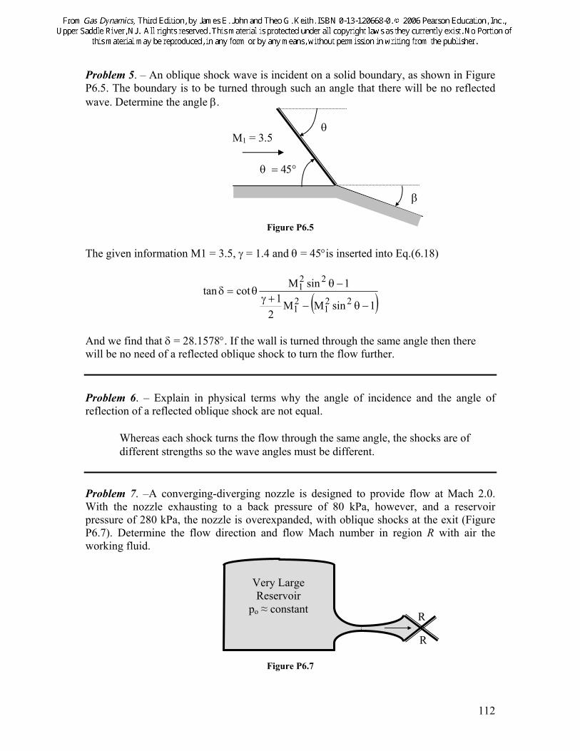
Problem 1. – Air is stored in a pressurized tank at a pressure of 120 kPa (gage) and a temperature of 27°C. The tank volume is 1 m3. Atmospheric pressure is 101 kPa and the local acceleration of gravity is 9.81 m/s2. (a) Determine the density and weight of the air in the tank, and (b) determine the density and weight of the air if the tank was located on the Moon where the acceleration of gravity is one sixth that on the Earth.

Kkg/kJ 728.0R s/m81.9g

m1

C30027327T

kpa 122101120PPP

2

3

atmgageabs

⋅==

=∀

°=+=

=+=+=

a) 3mkg5668.2

)300)(287.0(221

RTP

===ρ

N1801.25)81.9)(1)(5668.2(gmgW ==∀ρ==

b) 3earthmoonmkg5668.2=ρ=ρ

N1967.4W61W

gg

W earthearthearth

moonmoon ===

Problem 2. – (a) Show that p/ρ has units of velocity squared. (b) Show that p/ρ has the same units as h (kJ/kg). (c) Determine the units conversion factor that must be applied to kinetic energy, V2/2, (m2/s2) in order to add this term to specific enthalpy h (kJ/kg).

Air

2

a) 2

2

2

2

3

2

32

Vsm

sNmkg 1

kgmN

kgm

mNp

mkg ,

mNp

≈=⎟⎟⎠

⎞⎜⎜⎝

⎛

⋅

⋅−=⎟

⎟⎠

⎞⎜⎜⎝

⎛⎟⎟⎠

⎞⎜⎜⎝

⎛≈

ρ

⎟⎟⎠

⎞⎜⎜⎝

⎛≈ρ⎟⎟

⎠

⎞⎜⎜⎝

⎛≈

b) kgkJ

10001

J 0100kJ1

mNJ1

kgmNP

=⎟⎠⎞

⎜⎝⎛

⎟⎠⎞

⎜⎝⎛

⋅⋅

≈ρ

c)

c

2

2

22

g10001factor

kgkJ

J 0100kJ 1

mN J1

mkgsN1

sm

2V

=∴

≈⎟⎠⎞

⎜⎝⎛

⎟⎠⎞

⎜⎝⎛

⋅⎟⎟⎠

⎞⎜⎜⎝

⎛

⋅⋅

≈

Problem 3. – Air flows steadily through a circular jet ejector, refer to Figure 1.15. The primary jet flows through a 10 cm diameter tube with a velocity of 20 m/s. The secondary flow is through the annular region that surrounds the primary jet. The outer diameter of the annular duct is 30 cm and the velocity entering the annulus is 5 m/s. If the flows at both the inlet and exit are uniform, determine the exit velocity. Assume the air speeds are small enough so that the flow may be treated as an incompressible flow, i.e., one in which the density is constant. ei mm && = ssppspi VAVAmmm ρ+ρ=+= &&& eee VAm ρ=& eesspp VAVAVA =+∴ So

e

ssppe A

VAVAV

+=

pse AAA +=

2pp D

4A π

= 2p

2os D

4D

4A π

−π

= 2oe D

4A π

=

i e

s p

3

( ) ( )sp2o

2p

s2o

s2p

2op

2p

e

ssppe VV

D

DV

D

VDDVDA

VAVAV −+=

−+=

+=

( ) s/m6667.652030105 2

2=−+=

Problem 4. – A slow leak develops in a storage bottle and oxygen slowly leaks out. The volume of the bottle is 0.1 m3 and the diameter of the hole is 0.1 mm. The initial pressure is 10 MPa and the temperature is 20˚C. The oxygen escapes through the hole according to the relation

ee ATp04248.0m =&

where p is the tank pressure and T is the tank temperature. The constant 0.04248 is based on the gas constant and the ratio of specific heats of oxygen. The units are: pressure N/m2, temperature K, area m2 and mass flow rate kg/s. Assuming that the temperature of the oxygen in the bottle does not change with time, determine the time it takes to reduce the pressure to one half of its initial value. 3m 1.0=∀ MPa 01p1 = 21 TK293T == MPa 5p2 =

Kkg

J8219.25932

3.314,8R⋅

==

From the continuity equation

emdtdm

&−=

but

RTpm ∀

=

so

pT

A 80424.0m

dtdp

RTdtdm e

e −=−=∀

= &

Integrating we get,

O2

m(t)

d = 0.1mm

ee ATp04248.0m =&

4

tATR 80424.0

pp

ln e

1

2⎟⎟⎠

⎞⎜⎜⎝

⎛

∀−=

hrs 5979.12sec4076.713,46

21ln

293)8219.259(mm 0100

mmm 1.04

)04248.0(

1.0

pp

lnTRA)04248.0(

t

2

1

2

e

==

⎟⎠⎞

⎜⎝⎛

⎟⎠⎞

⎜⎝⎛

⎟⎠⎞

⎜⎝⎛ π

−=

∀−=

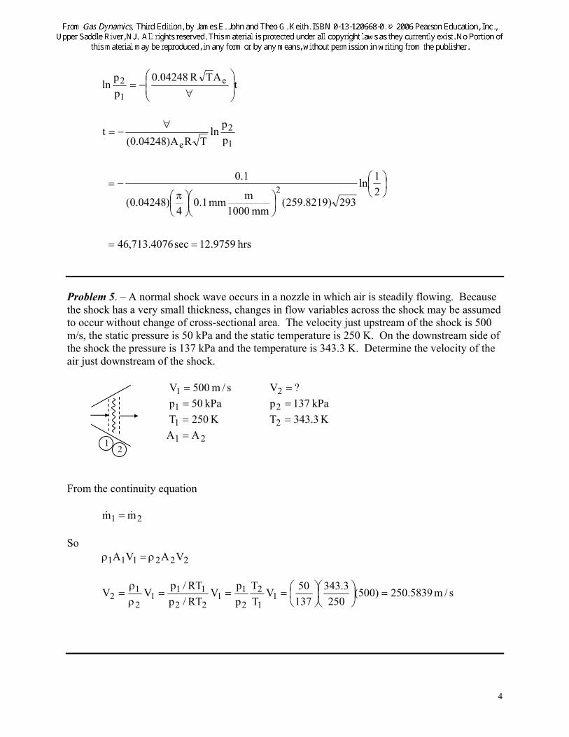
Problem 5. – A normal shock wave occurs in a nozzle in which air is steadily flowing. Because the shock has a very small thickness, changes in flow variables across the shock may be assumed to occur without change of cross-sectional area. The velocity just upstream of the shock is 500 m/s, the static pressure is 50 kPa and the static temperature is 250 K. On the downstream side of the shock the pressure is 137 kPa and the temperature is 343.3 K. Determine the velocity of the air just downstream of the shock. s/m 050V1 = ?V2 = kPa 05p1 = kPa 713p2 = K 025T1 = K 3.343T2 = 21 AA = From the continuity equation

21 mm && = So

222111 VAVA ρ=ρ

s/m5839.250)500(250

3.34313750V

TT

pp

VRT/pRT/p

VV 11

2

2

11

22

111

2

12 =⎟

⎠⎞

⎜⎝⎛

⎟⎠⎞

⎜⎝⎛===

ρρ

=

2 1

5

Problem 6. – A gas flows steadily in a 2.0 cm diameter circular tube with a uniform velocity of 1.0 cm/s and a density ρo. At a cross section farther down the tube, the velocity distribution is given by V = Uo[1-( r/R)2], with r in centimeters. Find Uo, assuming the gas density to be ρo[1+( r/R)2].

s/cm 1V1 = ⎥⎥⎦

⎤

⎢⎢⎣

⎡⎟⎠⎞

⎜⎝⎛−=

2

o2 Rr1UV

o1 ρ=ρ ⎥⎥⎦

⎤

⎢⎢⎣

⎡⎟⎠⎞

⎜⎝⎛+ρ=ρ

2

o2 Rr1

21 mm && =

o22

1oR

o 111R

o 11 RRVrdr2VdAVm ρπ=πρ=πρ=ρ= ∫∫&

( )

oo22

oo

1

o522

oo

2

2o2

2R

o

R

o o222

UR32

61

21RU2

Rr wheredR2U

rdr2Rr1U

Rr1dAVm

ρπ=⎟⎠⎞

⎜⎝⎛ −πρ=

=ξξξ−ξπρ=

π⎟⎟⎠

⎞⎜⎜⎝

⎛−⎟

⎟⎠

⎞⎜⎜⎝

⎛+ρ=ρ=

∫

∫ ∫&

oo2

o2 UR

32R ρ

π=ρπ∴

so s/cm23Vo =

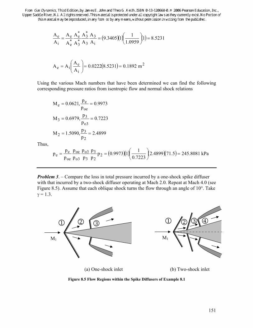
Problem 7. – For the rocket shown in Figure 1.6, determine the thrust. Assume that exit plane pressure is equal to ambient pressure.

( ) ( ) ( )ee

2oH

ee

oHoHeeeatme A

mmV

mmmm0VmApp

ρ+

=⎟⎟⎠

⎞⎜⎜⎝

⎛ρ

+++=+−=

&&&&&&&T

r

1 2

6

Problem 8. – Determine the force F required to push the flat plate of Figure Pl.8 against the round air jet with a velocity of 10 cm/s. The air jet velocity is 100 cm/s, with a jet diameter of 5.0 cm. Air density is 1.2 kg/m3.

Figure P1.8

To obtain steady state add + Vp to all velocities

VmF &=

( ) ( ) ( )1.015.04

2.1AVm 2 +⎟⎠⎞

⎜⎝⎛ π

=ρ=& s/kg 200259.0=

( )( ) N 100285.01.1002592.0F ==

Problem 9. – A jet engine (Figure P1.9) is traveling through the air with a forward velocity of 300 m/s. The exhaust gases leave the nozzle with an exit velocity of 800 m/s with respect to the nozzle. If the mass flow rate through the engine is 10 kg/s, determine the jet engine thrust. Exit plane static pressure is 80 kPa, inlet plane static pressure is 20 kPa, ambient pressure surrounding the engine is 20 kPa, and the exit plane area is 4.0 m2.

F

x V = -10 s

cm

Vj = 100 scm

Vj = 110 scm

x

V = 0

F

7

Figure P1.9 ( ) ( ) ( )( ) ( )( ) kN24552403008001042080VVmApp ieeatme =+=−+−=−+−= &T Problem 10. – A high-pressure oxygen cylinder, typically found in most welding shops, accidentally is knocked over and the valve on top of the cylinder breaks off. This creates a hole with a cross-sectional area of 6.5 x 10-4 m2. Prior to the accident, the internal pressure of the oxygen is 14 MPa and the temperature is 27˚C. Based on critical flow calculations, the velocity of the oxygen exiting the cylinder is estimated to be 300 m/s, the exit pressure 7.4 MPa and the exit temperature 250 K. How much thrust does the oxygen being expelled from the cylinder generate? What percentage is due to the pressure difference? What percentage due to the exiting momentum? Atmospheric pressure is 101 kPa. Also note that 0.2248 lbf = 1 N.

Figure P1.10

s/m 030Ve = 24e m105.6A −×=

MPa 4.7pe = MPa 110.0kPa 110patm ==

k 025Te = eee

eeee VA

RTp

VAm =ρ=&

kkgJ82.259R⋅

= ( )( ) ( )( ) s/kg2.22300105.625082.259mN104.7

426

=×⎟⎟⎠

⎞⎜⎜⎝

⎛×

= −

300 m/s 800 m/s

8

( )

( ) ( )( )

( )

f

2

243

eeatme

lb3.548,2N0.336,11

N6.66644.4671

mkgsN1

smkg3002.22N104.6101017400

VmApp

==

+=

⎟⎟⎠

⎞⎜⎜⎝

⎛

⋅⋅

⎟⎟⎠

⎞⎜⎜⎝

⎛ ⋅+×××−=

+−=

−

&T

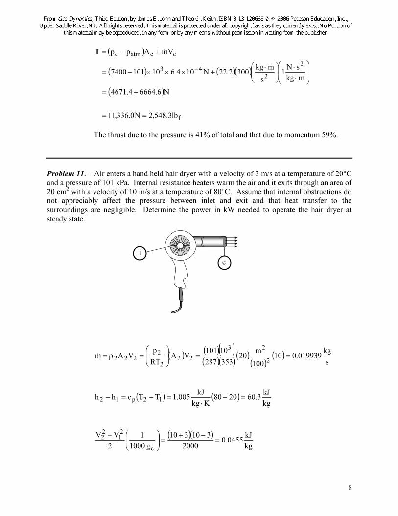
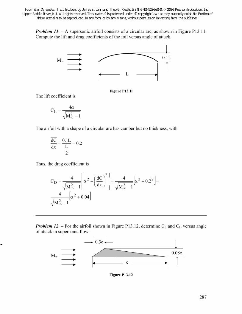
The thrust due to the pressure is 41% of total and that due to momentum 59%. Problem 11. – Air enters a hand held hair dryer with a velocity of 3 m/s at a temperature of 20°C and a pressure of 101 kPa. Internal resistance heaters warm the air and it exits through an area of 20 cm2 with a velocity of 10 m/s at a temperature of 80°C. Assume that internal obstructions do not appreciably affect the pressure between inlet and exit and that heat transfer to the surroundings are negligible. Determine the power in kW needed to operate the hair dryer at steady state.

( ) ( )( )( )( ) ( )

( )( )

skg019939.010

100m20

35328710101VA

RTp

VAm 2

2322

2

2222 ==⎟⎟

⎠

⎞⎜⎜⎝

⎛=ρ=&

( ) ( )kgkJ3.602080

KkgkJ005.1TTchh 12p12 =−⋅

=−=−

( )( )kgkJ0455.0

2000310310

g 01001

2VV

c

21

22 =

−+=⎟⎟

⎠

⎞⎜⎜⎝

⎛−

i e

9

⎟⎟

⎠

⎞

⎜⎜

⎝

⎛+−⎟

⎟

⎠

⎞

⎜⎜

⎝

⎛+=−

2V

hm2

VhmWQ

21

1

22

2 &&&&

( ) ( )( )

W2051.203,1kgkJ203205.1

0455.03.60019939.02

VVhhmW2

122

12

==

+=⎥⎥⎦

⎤

⎢⎢⎣

⎡

⎟⎟⎠

⎞⎜⎜⎝

⎛ −+−=− &&

Problem 12. – Air is expanded isentropically in a horizontal nozzle from an initial pressure of 1.0 MPa, of a temperature of 800 K, to an exhaust pressure of 101 kPa. If the air enters the nozzle with a velocity of 100 m/s, determine the air exhaust velocity. Assume the air behaves as a perfect gas, with R = 0.287 kJ/kg · K and γ = 1.4. Repeat for a vertical nozzle with exhaust plane 2.0 m above the intake plane.

(a) Horizontal nozzle

2V

h2

Vhh

22

2

21

1o +=+=

( ) ( )212

121p2

12 TT1

R2VTTc 2VV −−γγ

+=−+=

kkgJ287R⋅

=

5194.01000101

pp

TT 4.1

4.1

1

2

1

2 =⎟⎠⎞

⎜⎝⎛=⎟⎟

⎠

⎞⎜⎜⎝

⎛=

γ−γ

K 5.415T2 =

( ) ( )( )( ) ( ) s/m 856.8845.460,772000,105.4158004.0

2874.12100V 22 =+=−+=

(b) Vertical nozzle

1 2

p2 = 101kPa p1 = 1MPa T1 = 800K V1 = 100m/s

10

2

22

21

21

1 gz2

Vhgz

2V

h ++=++

( ) ( ) ( )( )( )281.925.460,782zzg2TT1

R2VV 21212

12 +=−+−−γγ

+=

s/m 059.88474.499,782 ==

Problem 13. – Nitrogen is expanded isentropically in a nozzle from a pressure of 2000 kPa, at a temperature of 1000 K, to a pressure of 101 kPa. If the velocity of the nitrogen entering the nozzle is negligible, determine the exit nozzle area required for a nitrogen flow of 0.5 kg/s. Assume the nitrogen to behave as a perfect gas with constant specific heats, mean molecular mass of 28.0, and γ = 1.4.

2V

h2

Vhh

22

2

21

1o +=+=

( ) ( )21p212 TTc 2hh2V −=−=

( ) K1.42620001011000

PPTT 4.1

4.01

1

212 =⎟

⎠⎞

⎜⎝⎛=⎟⎟

⎠

⎞⎜⎜⎝

⎛=

γ−γ

Kkg

J9.29628

3.8314R⋅

==

( ) ( ) ( )( )( ) s/m2.10921.42610009.2967TTR7TT1

R2V 21212 =−=−=−−γ

γ=

( )( ) 32

22

mkg798.0

1.4269.296000,101

RTp

===ρ

p1 = 2000kPa T1 = 1000K V1 ~ small

1 2

p2 = 101kPa

m = 0.5kg/s = ρ2A2V2 •

A2 = ?

V2 = ?

11

( )( )22

222 cm 473.5m 4000573.0

2.1092798.05.0

VmA ===

ρ=

&

Problem 14. – Air enters a compressor with a pressure of 100 kPa and a temperature 20°C; the mass flow rate is 0.25 kg/s. Compressed air is discharged from the compressor at 800 kPa and 50°C. Inlet and exit pipe diameters are 4.0 cm. Determine the exit velocity of the air at the compressor outlet and the compressor power required. Assume an adiabatic, steady, flow and that the air behaves as a perfect gas with constant specific heats; cp = 1.005 kJ/kg · K and R = 0.287kJ/kg·K.

kgkJ005.1cp =

kkgkJ287.0R

⋅=

s/kg 52.0mmm 21 === &&&

( ) 22221 m 60012.004.0

4d

4AA =

π=

π==

( )( ) 31

11

mkg189.1

2930.287kPa 0.10

RTp

===ρ

( )( ) 31

22

mkg630.8

3230.287800

RTp

===ρ

( )( ) sm3.167

00126.189.125.0

AmV

111 ==

ρ=

&

( )( ) sm1.23

00126.63.825.0

AmV

222 ==

ρ=

&

p1 = 100kPa T1 = 293K

d = 4.cm

1

2

W = ? •

m = 0.25 kg/s •

p2 = 800KPa T2 = 323K

V2 = ?

12

⎟⎟

⎠

⎞

⎜⎜

⎝

⎛+−⎟

⎟

⎠

⎞

⎜⎜

⎝

⎛+=−

2V

hm2

VhmWQ

21

11

22

22 &&&&

( )⎥⎥⎦

⎤

⎢⎢⎣

⎡ −+−=−

2VV

hhmW2

122

12&&

( ) ( )( ) ( )( )( )( ) ⎥

⎦

⎤⎢⎣

⎡ −++−=

1000216731.231.233.167293323005.125.0

( )( ) kW 1.4skJ1.473.1315.3025.0 ==−=

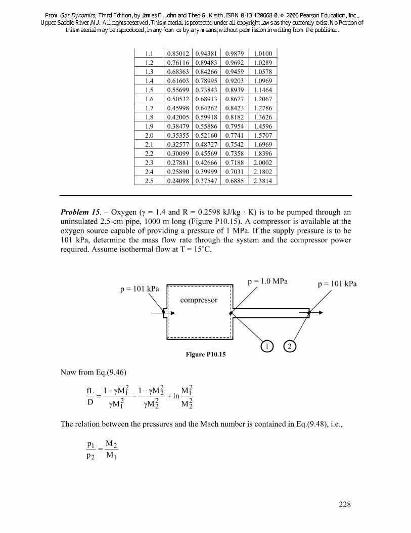
Problem 15. – Hot gases enter a jet engine turbine with a velocity of 50 m/s, a temperature of 1200 K, and a pressure of 600 kPa. The gases exit the turbine at a pressure of 250 kPa and a velocity of 75 m/s. Assume isentropic steady flow and that the hot gases behave as a perfect gas with constant specific heats (mean molecular mass 25, γ = 1.37). Find the turbine power output in kJ/(kg of mass flowing through the turbine).

KkgJ6.332

253.8314R

⋅== 37.1=γ ( )( )

KkgkJ2314.1

37.6.33237.1

1Rcp ⋅

==−γ

γ=

K 3.9476002501200

ppTT 37.1

37.01

1

212 =⎟

⎠⎞

⎜⎝⎛=⎟⎟

⎠

⎞⎜⎜⎝

⎛=

γ−γ

1

2

W •

V1 = 50m/s T1 = 1200K p1 = 600kPa

p2 = 250 kPa V2 = 75 m/s

13

⎟⎟

⎠

⎞

⎜⎜

⎝

⎛+−⎟

⎟

⎠

⎞

⎜⎜

⎝

⎛+=−

2V

hm2

VhmWQ

21

11

22

22 &&&&

( )⎥⎥⎦

⎤

⎢⎢⎣

⎡ −+−=

2VV

hhmW22

21

21&&

( ) ( )( )2000

VVVVTTc2

VVhhmWW 2121

21p22

21

21−+

+−=−

+−==&

&

( )( ) ( )( )kgkJ6.309563.118.311

2000251253.94712002314.1W =−=⎟

⎠⎞

⎜⎝⎛ −

+−=

Problem 16. – Hydrogen is stored in a tank at 1000 kPa and 30°C. A valve is opened, which vents the hydrogen and allows the pressure in the tank to fall to 200 kPa. Assuming that the hydrogen that remains in the tank has undergone an isentropic process, determine the amount of hydrogen left in the tank. Assume hydrogen is a perfect gas with constant specific heats; the ratio of specific heats is 1.4, and the gas constant is 4.124 kJ/kg · K. The tank volume is 2.0m3.

K303TkPa 1000p 11 ==

kPa 200p2 = ( ) K3.1911000200303

ppTT 4.1

4.01

1

212 =⎟

⎠⎞

⎜⎝⎛=⎟⎟

⎠

⎞⎜⎜⎝

⎛=

γ−γ

( )( )( )( ) kg 507.0

3.191124.42200

RTpm

2

22 ==

∀=

14

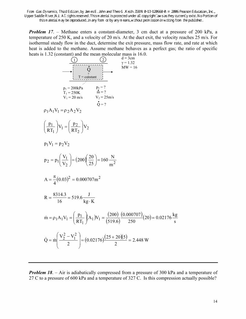
Problem 17. – Methane enters a constant-diameter, 3 cm duct at a pressure of 200 kPa, a temperature of 250 K, and a velocity of 20 m/s. At the duct exit, the velocity reaches 25 m/s. For isothermal steady flow in the duct, determine the exit pressure, mass flow rate, and rate at which heat is added to the methane. Assume methane behaves as a perfect gas; the ratio of specific heats is 1.32 (constant) and the mean molecular mass is 16.0.

222111 VAVA ρ=ρ

22

21

1

1 V RTpV

RTp

⎟⎟⎠

⎞⎜⎜⎝

⎛=⎟⎟

⎠

⎞⎜⎜⎝

⎛

2211 VpVp =

( )22

112

mN 160

2520200

VV

pp =⎟⎠⎞

⎜⎝⎛=⎟⎟

⎠

⎞⎜⎜⎝

⎛=

( ) 22 m000707.003.04

A =π

=

Kkg

J519.616

3.8314R⋅

==

( ) ( )( )

( ) ( )s

kg02176.020250

000707.06.519

200VARTp

VAm 111

1111 ==⎟⎟

⎠

⎞⎜⎜⎝

⎛=ρ=&

( ) ( )( ) W 448.22

5202502176.02

VVmQ

21

22 =

+=⎟

⎟

⎠

⎞

⎜⎜

⎝

⎛ −= &&

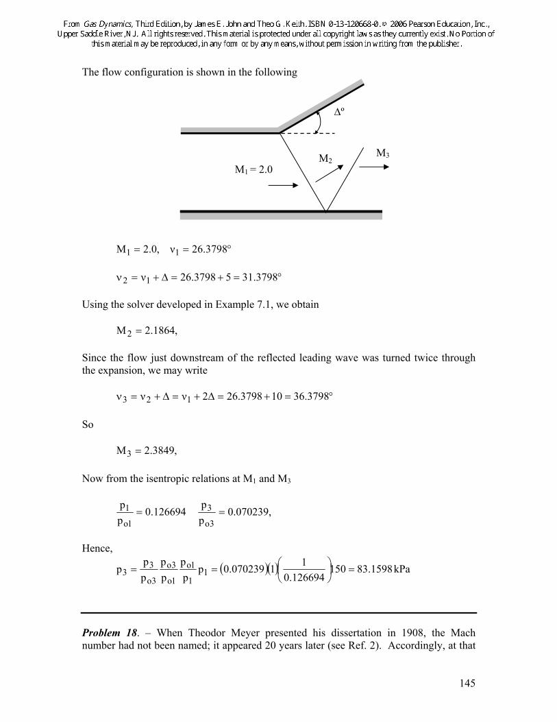
Problem 18. – Air is adiabatically compressed from a pressure of 300 kPa and a temperature of 27 C to a pressure of 600 kPa and a temperature of 327 C. Is this compression actually possible?

1 2

T = constant

Q •

p1 = 200kPa T1 = 250K V1 = 20 m/s

p2 = ? m = ? •

V2 = 25m/s

Q = ? •

d = 3cm γ = 1.32 MW = 16

15

kPa 300p1 = kPa 600p2 = K30027327T1 =+= K600273327T2 =+=

300600lnR

300600lnc

pplnR

TTlncss p

1

2

1

2p12 −=−=−

( ) 02lnc2lnRc vp >=−= possible∴ Problem 19. – Two streams of air mix in a constant-area mixing tube of a jet ejector. The primary jet enters the tube with a speed of 600 m/s, a pressure of 200 kPa and a temperature of 400˚C. The secondary stream enters with a velocity of 30 m/s, a pressure of 200 kPa and a temperature of 100˚C. The ratio of the area of the secondary flow to the primary jet is 5:1. The air behaves as a perfect gas with constant specific heats, cp = 1.0045 kJ/kg· K. Using the iterative numerical procedure described in Example 1.9 determine the velocity, pressure and temperature of the air leaving the mixing tube.

gc 1 α 5 γ 1.4 R 287 cp 1004.5 Primary Secondary

V 600.00 30.00 T 673 373 P 200,000 200,000

A 43,122.5078

B 263,528.7595

C 706,538.5693 n Ve (m/s) Pe (Pa) Te (K) 1 0.0000 101,000.0 293.1500 2 125.1620 244,722.8 695.5757 3 122.5671 245,112.7 695.8957 4 122.4284 245,133.6 695.9126 5 122.4210 245,134.7 695.9135 6 122.4206 245,134.7 695.9136 7 122.4206 245,134.7 695.9136

16

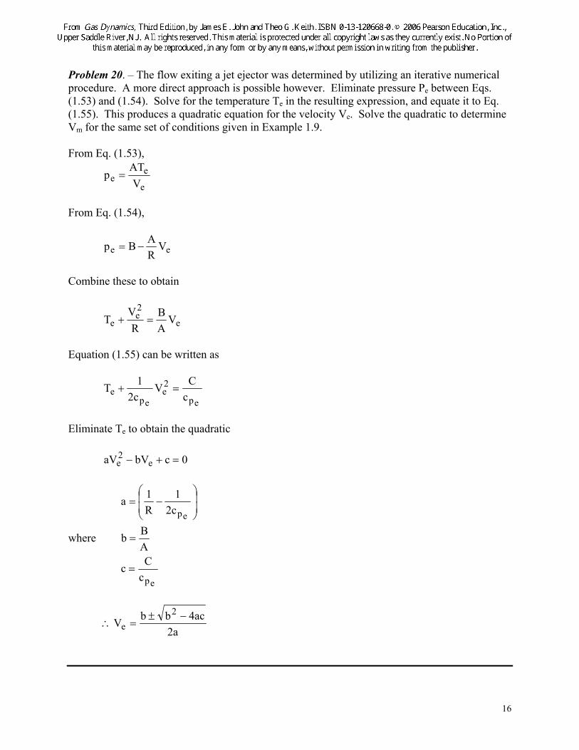
Problem 20. – The flow exiting a jet ejector was determined by utilizing an iterative numerical procedure. A more direct approach is possible however. Eliminate pressure Pe between Eqs. (1.53) and (1.54). Solve for the temperature Te in the resulting expression, and equate it to Eq. (1.55). This produces a quadratic equation for the velocity Ve. Solve the quadratic to determine Vm for the same set of conditions given in Example 1.9. From Eq. (1.53),

e

ee V

ATp =

From Eq. (1.54),

ee VRABp −=

Combine these to obtain

e2e

e VAB

RV

T =+

Equation (1.55) can be written as

ep

2e

epe c

CVc21T =+

Eliminate Te to obtain the quadratic

0cbVaV e2e =+−

where

ep

ep

cCc

ABb

c21

R1a

=

=

⎟⎟⎠

⎞⎜⎜⎝

⎛−=

a2

ac4bbV2

e−±

=∴

17

CChhaapptteerr TTwwoo

WWAAVVEE PPRROOPPAAGGAATTIIOONN IINN CCOOMMPPRREESSSSIILLBBEE MMEEDDIIAA

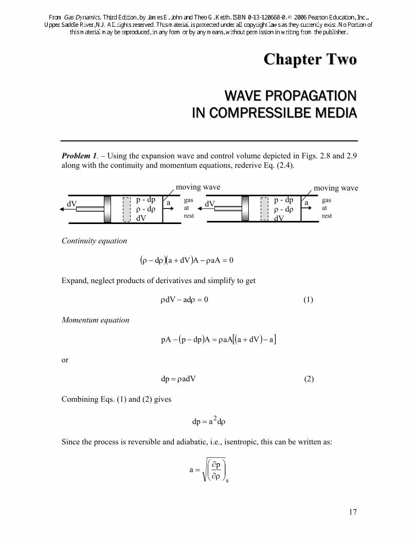
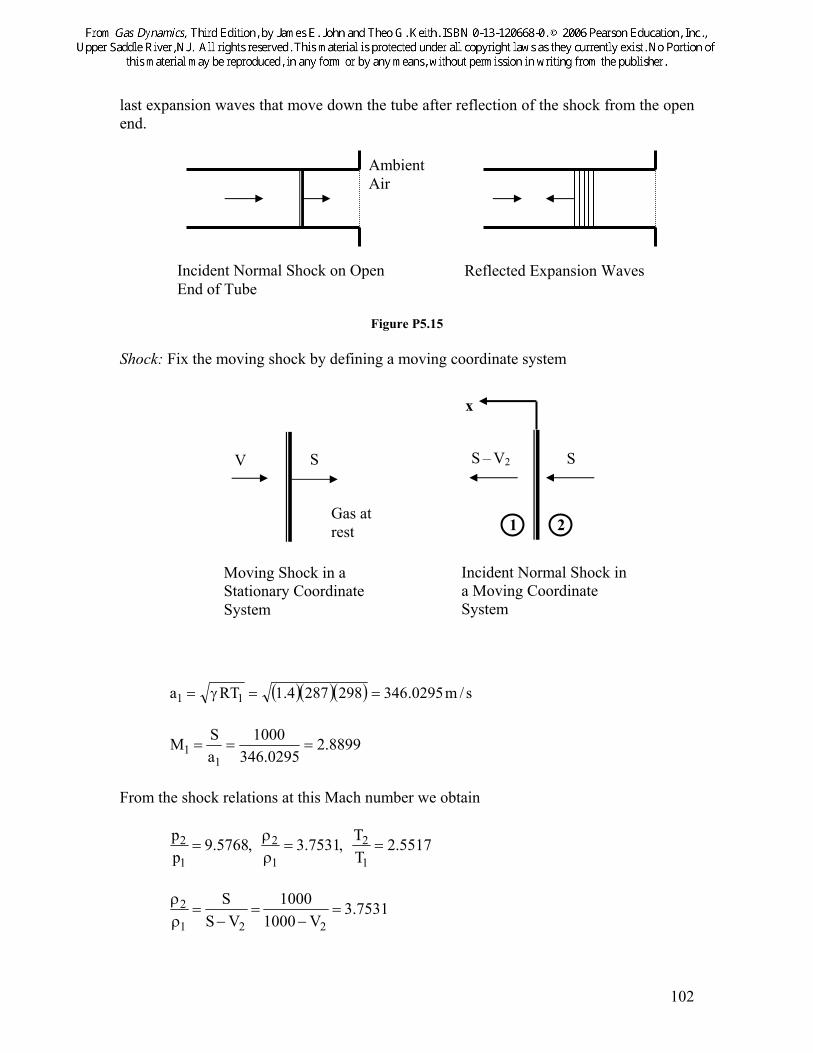
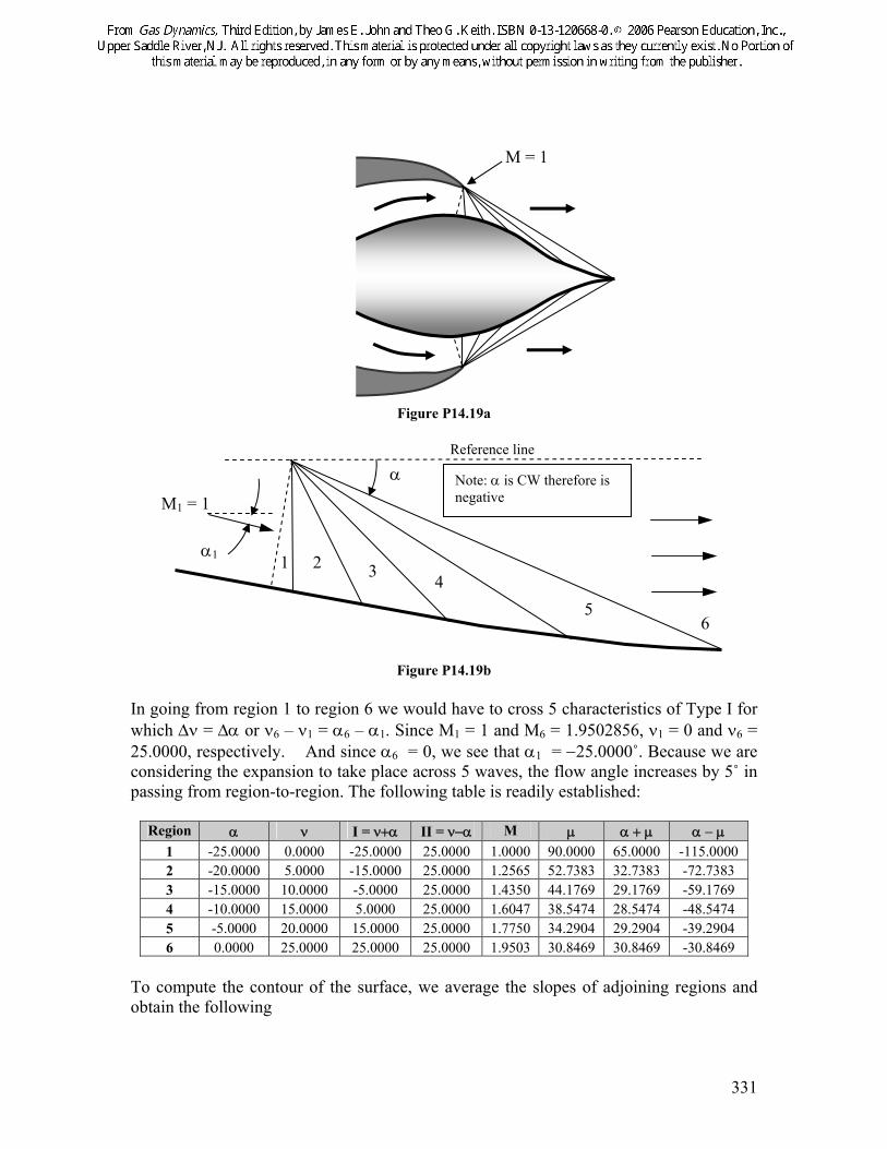
Problem 1. – Using the expansion wave and control volume depicted in Figs. 2.8 and 2.9 along with the continuity and momentum equations, rederive Eq. (2.4). Continuity equation ( )( ) 0aAAdVad =ρ−+ρ−ρ Expand, neglect products of derivatives and simplify to get

0addV =ρ−ρ (1)

Momentum equation

( ) ( )[ ]adVaaAAdpppA −+ρ=−−

or

adVdp ρ= (2)

Combining Eqs. (1) and (2) gives

ρ= dadp 2 Since the process is reversible and adiabatic, i.e., isentropic, this can be written as:

s

pa ⎟⎟⎠

⎞⎜⎜⎝

⎛ρ∂

∂=

a gas at rest

p - dp ρ - dρ dV

moving wave

dV a gas at rest

p - dp ρ - dρ dV

moving wave

dV

18

Problem 2. – (a) Derive an expression for ks, for a perfect gas, substitute the result into Eq. (2.10), and thereby demonstrate Eq. (2.7); (b) Derive an expression for kT, for a perfect gas, substitute the result into Eq. (2.11), and thereby demonstrate Eq. (2.7) and finally; (c) Derive an expression for βs, for a perfect gas, substitute your result into Eq. (2.14), and thereby demonstrate Eq. (2.7).

(a) s

s p1k ⎟⎟

⎠

⎞⎜⎜⎝

⎛∂ρ∂

ρ=

An isotropic process involving a perfect gas is described by γρ= cP

ργ

=ρργ

=ργ=ρ

∴γ

−γ pccddp 1

Hence,

pp s γρ

=⎟⎟⎠

⎞⎜⎜⎝

⎛∂ρ∂

RT1

p1

p1k

ss ργ

=γ

=⎟⎟⎠

⎞⎜⎜⎝

⎛∂ρ∂

ρ=

So,

RTk1a

sγ=

ρ=

(b) T

T p1k ⎟⎟

⎠

⎞⎜⎜⎝

⎛∂ρ∂

ρ=

RTp

=ρ

RT1

p T=⎟⎟

⎠

⎞⎜⎜⎝

⎛∂ρ∂

RT1kT ρ

=

So,

19

RTk

aT

γ=ρ

γ=

(c) RTppp

ss γρ=γ=⎟⎟

⎠

⎞⎜⎜⎝

⎛ργ

ρ=⎟⎟⎠

⎞⎜⎜⎝

⎛ρ∂

∂ρ=β

RTa s γ=ρ

β=

Problem 3. – Use dimensional analysis to develop an expression for the speed of sound in terms of the isentropic compressibility, the density and gc.

( )es g,,kfa ρ=

2c3

2s

FTML~g,

LM~,

FL~k,

TL~a ρ

c2cb3a2cbcac

2

b

3

a2TLMF

FTML

LM

FL

TL −+−+−−=⎟⎟

⎠

⎞⎜⎜⎝

⎛⎟⎟⎠

⎞⎜⎜⎝

⎛⎟⎟⎠

⎞⎜⎜⎝

⎛=

1c2:T1cb3a2:L

0cb:M0ca:F

=−=+−

=+=−−

Hence, 21b

21a

21c −=−==

So,

s

ck

ga

ρ=

Problem 4. – Using the data provided in Tables 2-1, 2-2 and 2-3, i.e., the density, and the isentropic compressibility or the bulk modulus, calculate the velocity of sound at 20°C and one atmosphere pressure in (a) helium, (b) turpentine, and (c) lead.

(a) Helium: 3mkg16.0=ρ ,

GPa1919,5ks =

20

)919,5)(16.0(10

k1a

9

s

=ρ

= s/m 6.1027=

(b) Turpentine: 3mkg870=ρ ,

GPaks

1736.0=

)736.0)(870(10

k1a

9

s=

ρ= s/m 7.1249=

(c) Lead: 3mkg300,11=ρ , GPa 72.16s =β

300,1110 )27.16(a

9s =

ρβ

= s/m 9.1199=

Problem 5. – In Example Problem 2.3 the speed of sound of superheated steam was determined by using a finite difference representation of the compressibility and steam table data (Table 2-4). Using the same steam table data, determine the speed of sound of superheated steam for the same pressure and temperature, i.e., at p = 500 kPa and T = 300˚C. However, use the following finite differences to obtain two estimates for the speed of sound:

( )TT

2

pv1

p

a

⎥⎦

⎤⎢⎣

⎡∂

∂γ

=

⎟⎟⎠

⎞⎜⎜⎝

⎛∂ρ∂γ

=

( )ss

2

pv1

1

p

1a

⎥⎦

⎤⎢⎣

⎡∂

∂=

⎟⎟⎠

⎞⎜⎜⎝

⎛∂ρ∂

=

( )( ) ( ) ( ) ( )T,ppv

1T,ppv

1p2

p2T,ppv

1T,ppv

1pv1

a

T

2

∆−−

∆+

∆γ=

∆∆−

−∆+

γ=

⎥⎦

⎤⎢⎣

⎡∂

∂γ

=

From Example 2.3

( )kgM4344.0Tppv

31 =∆+ , ( )

kgM6548.0Tppv

31 =∆− , and Pa 000,100p =∆

21

( )( )( )2

22

sm5.521,342

6548.01

4344.01

000,100327.12a =−

=

s/m 3.585a =

( )( ) ( )s,ppv

1s,ppv

1p2

pv1

1a

s

2

∆−−

∆+

∆=

⎥⎦

⎤⎢⎣

⎡∂

∂=

From Example 2.3

( )kgM4544.0s,ppv

3=∆+ , ( )

kgM6209.0s,ppv

3=∆− and Pa 000,100p =∆

( )( )2

22

sm2.903,338

6209.01

4544.01

000,1002a =−

=

s/m 2.582a =

Problem 6. – Equation (2.16) provides a convenient expression for calculating the speed of sound in air: a = 20.05 T , where T is the absolute temperature in degrees Kelvin. Derive the following linear equation for the speed of sound in air:

0 t6.0aa += where a0 is the speed of sound in air at 0°C and t is °C. To accomplish this make use of Eq. (2-16) and the expansion

( ) .....ynxxyx 1nnn ++=+ − ( )[ ] t273RRTa 2/1+γ=γ=

⎟⎠⎞

⎜⎝⎛ ++=⎟

⎠⎞

⎜⎝⎛ +γ= .....

273t

211a

273t1)273(R o

2/1

22

( )

( )( ) 6.0546331

2732a

,sm 13327305.20273Ra

o

o

==

==γ=

t6.0331a +=∴

Problem 7. – Rather than measure the bulk modulus directly it may be easier to measure the speed of sound as it propagates though a material and then use it to compute the bulk modulus. For a Lucite plastic of density 1,200 kg/m3, the speed of sound is measured as 2,327 m/s. Determine the bulk modulus. What is the corresponding isentropic compressibility?

Now 3mkg200,1=ρ ,

sm327,2a =

ρ

β= sa

so, GPa 849.6Pa10498.6mkgsN1

sm327,2

mskg200,1a 9

222

3 =×=⎟⎟⎠

⎞⎜⎜⎝

⎛⋅⋅

⎟⎠⎞

⎜⎝⎛

⎟⎠⎞

⎜⎝⎛=ρ=β

GPa11539.01k

ss =

β=

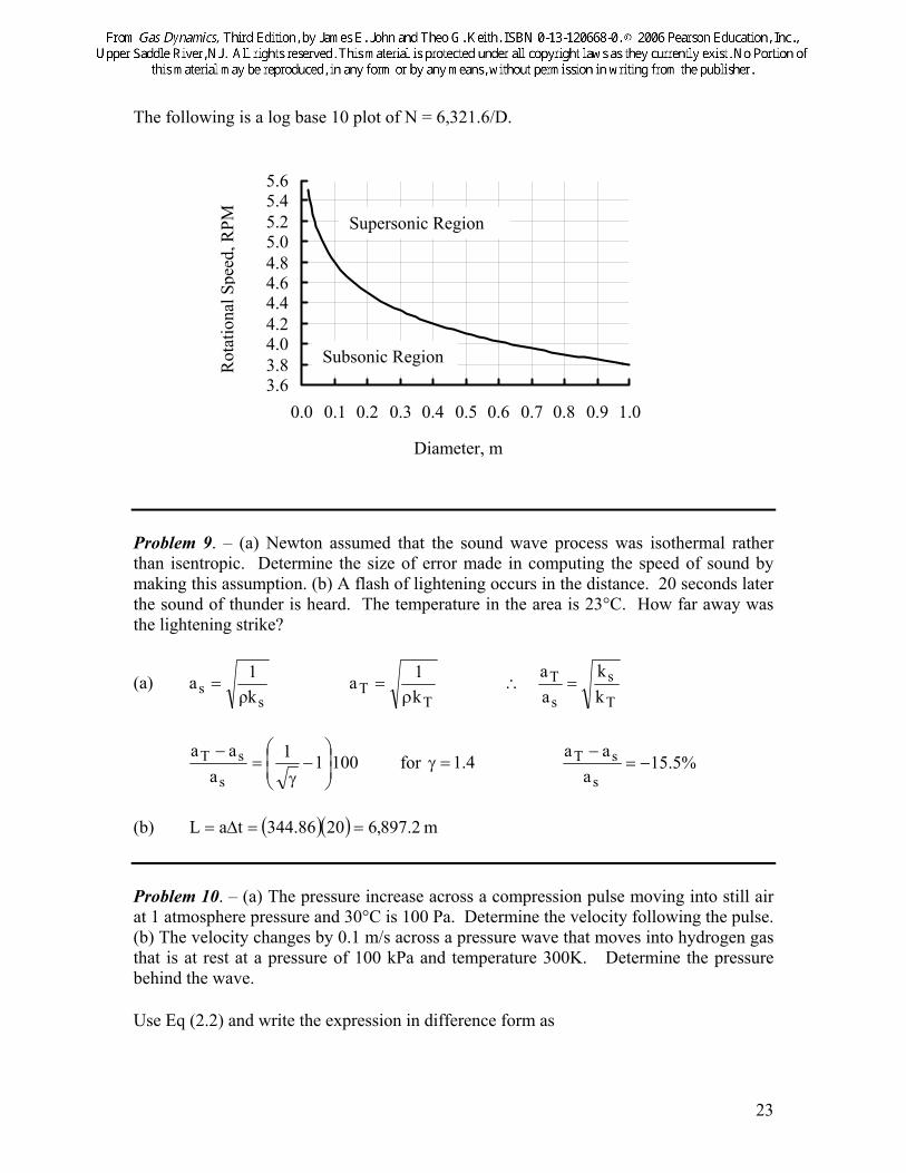
Problem 8. – An object of diameter d (m) is rotated in air at a speed of N revolutions per minute. Draw a plot of the rotational speed required for the velocity at the outer edge of the object to just reach sonic velocity for a given diameter. Take the speed of sound of the air to be 331m/s. The highest speed will occur at R.

( )sm331a

s 06min 1mR

revrad2

minrevNV ==⎟

⎠⎞

⎜⎝⎛ π

⎟⎠⎞

⎜⎝⎛=

sm,ND

60π

=

23

The following is a log base 10 plot of N = 6,321.6/D.

3.63.84.04.24.44.64.85.05.25.45.6

0.0 0.1 0.2 0.3 0.4 0.5 0.6 0.7 0.8 0.9 1.0

Problem 9. – (a) Newton assumed that the sound wave process was isothermal rather than isentropic. Determine the size of error made in computing the speed of sound by making this assumption. (b) A flash of lightening occurs in the distance. 20 seconds later the sound of thunder is heard. The temperature in the area is 23°C. How far away was the lightening strike?

(a) s

s ρk1a =

TT k

1aρ

= T

s

s

Tkk

aa

=∴

001 11a

aa

s

sT⎟⎟⎠

⎞⎜⎜⎝

⎛−

γ=

− for 4.1=γ %5.15

aaa

s

sT −=−

(b) ( )( ) m 2.897,620344.86taL ==∆= Problem 10. – (a) The pressure increase across a compression pulse moving into still air at 1 atmosphere pressure and 30°C is 100 Pa. Determine the velocity following the pulse. (b) The velocity changes by 0.1 m/s across a pressure wave that moves into hydrogen gas that is at rest at a pressure of 100 kPa and temperature 300K. Determine the pressure behind the wave. Use Eq (2.2) and write the expression in difference form as

Supersonic Region

Subsonic Region Rot

atio

nal S

peed

, RPM

Diameter, m

24

(a) ρa

p∆V =∆ , Pa 100∆p =

air: ( )

3mkg1615.1

30397.28

8314000,101ρ =⎟⎠⎞

⎜⎝⎛

=

m/s 0.34930305.20a ==

Therefore, ( )( ) m/s 247.00.3491615.1

100V ==∆

(b) ρa∆V∆p = , m/s 1.0V =∆

hydrogen: ( )

3mkg0808.0

300016.2

8314000,100

RTpρ =

⎟⎠⎞

⎜⎝⎛

==

( ) ( ) m/s 8.1320300016.1

831441.1a =⎟⎠⎞

⎜⎝⎛=

Therefore, ( )( )( ) Pa 68.101.08.13200808.0p ==∆ Problem 11. – (a) Helium at 35°C is flowing at a Mach number of 1.5. Find the velocity and determine the local Mach angle. (b) Determine the velocity of air at 40°C to produce a Mach angle of 38° (a) helium: K308C35T =°= 5.1M =

aMV = ( ) ( ) m/s 7.032,1308003,4314,8667.1RTa =⎟

⎠

⎞⎜⎝

⎛=γ=

( )( ) m/s 0.549,15.17.032,1V ==

°=⎟⎟⎠

⎞⎜⎜⎝

⎛µ

=µ − 8.411ins 1

(b) air: K313C40 =°=T m/s 6.2993.22305.20a ==

25

⎟⎠⎞

⎜⎝⎛=µ −

M1ins 1

aV

ins1M =

µ=

( ) m/s 0.57638ins

6.354insaV ==

µ=

Problem 12. – (a) A jet plane is traveling at Mach 1.8 at an altitude of 10 km where the temperature is 223.3K. Determine the speed of the plane. (b) Air at 320 K flows in a supersonic wind tunnel over a 2-D wedge. From a photograph the Mach angle is measured to be 45°. Determine the flow velocity, the local speed of sound and the Mach number of the tunnel. (a) 8.1M = , K 3.223T = , m/s 6.2993.22305.20a == ( )( ) m/s 3.5398.16.299aMV === (b) air: °=µ= 45,K 320T , m/s 7.35832005.20a ==

( ) m/s 2.50745ins7.358

insaV ==

µ=

414.1sin

1aVM =

µ==

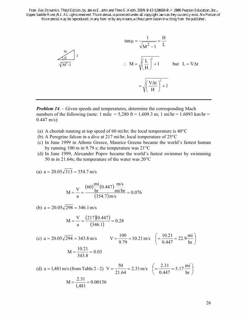
Problem 13. – A supersonic aircraft, flying horizontally a distance H above the earth, passes overhead. ∆t later the sound wave from the aircraft is heard. In this time increment, the plane has traveled a distance L. Show that the Mach number of the aircraft can be computed from:

1H

tV1HLM

22

+⎟⎠⎞

⎜⎝⎛ ∆

=+⎟⎠⎞

⎜⎝⎛=

Hint: first show that the Mach angle µ can be expressed as ⎟⎠⎞⎜

⎝⎛ −− 1M1tan 21 and then

connect the Mach angle, µ, to the geometric parameters H and L.

M1sin =µ

H

L µ

µ

26

LH

1M

1tan2

=−

=µ

t∆VLt bu 1HLM

2

=+⎟⎠⎞

⎜⎝⎛=∴

1H

t∆V 2

+⎟⎠⎞

⎜⎝⎛=

Problem 14. – Given speeds and temperatures, determine the corresponding Mach numbers of the following (note: 1 mile = 5,280 ft = 1,609.3 m; 1 mi/hr = 1.6093 km/hr = 0.447 m/s): (a) A cheetah running at top speed of 60 mi/hr; the local temperature is 40°C (b) A Peregrine falcon in a dive at 217 mi/hr; local temperature of 25°C (c) In June 1999 in Athens Greece, Maurice Greene became the world’s fastest human

by running 100 m in 9.79 s; the temperature was 21°C (d) In June 1999, Alexander Popov became the world’s fastest swimmer by swimming

50 m in 21.64s; the temperature of the water was 20°C (a) m/s 7.35431305.20a ==

( ) ( )

( ) 076.0m/s 7.354

mi/hrm/s447.0

hrmi60

aVM ===

(b) m/s 1.34629805.20a ==

( )( )( ) 28.0

1.346447.0217

aVM ===

(c) m/s 8.34329405.20a == m/s 21.1097.9

100V == ⎟⎠⎞

⎜⎝⎛ ==

hrmi9.22

447.021.10

03.08.343

21.10M ==

(d) 2)-2 Table (from m/s 481,1a = m/s 31.221.64

50V == ⎟⎠⎞

⎜⎝⎛ ==

hrmi17.5

447.031.2

00156.0481,131.2M ==

1 µ M

M2 -1

27

Problem 15. – Given speeds and Mach numbers, assuming air is a perfect gas, determine the corresponding local temperature (note: 1 mi/hr = 0.447 m/s) for the following:

(a) A Boeing 747-400 at a cruise speed of 910 km/hr; M = 0.85. (b) Concorde at a cruise speed of 1,320 mi/hr; M = 2.0 (c) The fastest airplane, the Lockheed SR-71 Blackbird, flying at 2,200 mi/hr; M =

3.3 (d) The fastest boat, the Spirit of Australia, that averaged 317.6 mi/hr; M = 0.41 (e) The fastest car, the ThrustSSC, averaged 760.035 mi/hr; M = 0.97

(a) sm8.252

s3600m000,910V == 85.0M =

sm4.297

85.8.252

MVa ===

C53K22005.204.297

05.20aT

22°−=°=⎟

⎠⎞

⎜⎝⎛=⎟

⎠⎞

⎜⎝⎛=

(b) ( )( ) sm0.590447.01320V == 0.2M = m/s 0.295

MVa ==

C5.56K5.21605.20

29505.20

aT22

°−==⎟⎠⎞

⎜⎝⎛=⎟

⎠⎞

⎜⎝⎛=

(3) ( )( ) sm4.983447.02200V == 3.3M = m/s 0.298

3.34.983a ==

C1.52K9.22005.200.298

05.20aT

22

°−==⎟⎠⎞

⎜⎝⎛=⎟

⎠⎞

⎜⎝⎛=

(d) ( )( ) sm0.142447.06.317V == 41.0M = m/s 3.346

41.142a ==

C2.25K2.29805.203.346

05.20aT

22°==⎟

⎠⎞

⎜⎝⎛=⎟

⎠⎞

⎜⎝⎛=

(e) ( )( ) m/s 7.339447.0035.760V == 97.0M = m/s 2.35097.

7.339a ==

C1.32K1.30505.202.350

05.20aT

22°==⎟

⎠⎞

⎜⎝⎛=⎟

⎠⎞

⎜⎝⎛=

28

Problem 16. – A baseball, which has a mass of 145 grams and a diameter of 3.66 cm, when dropped from a very tall building reaches high speeds. If the building is tall enough the speed will be controlled by the drag, as the baseball will reach terminal speed. At this state

DFW = Where W (weight) = mg, g (acceleration of gravity) = 9.81 m/s2, FD (drag force) = CDρairAV2/2, CD (drag coefficient) = 0.5 and A (projected area of sphere) = πR2. Find the terminal speed of the baseball and determine the corresponding Mach number if the ambient air temperature is 23°C and the ambient air pressure is 101 kPa..

The density of the air is first determined:

( )( )3

air m/kg19.1296287.0

101RTp

===ρ

Now

2VAC

FmgW2

airDD

ρ===

Hence,

( )( )

( )( )( ) s/m76.330042.019.15.081.9145.02

ACmg2V

airD==

ρ=

( )( )( )

098.02962874.1

76.33aVM ===

Problem 17. – Derive the following equation for the speed of sound of a real gas from Berthelot’s equation of state:

T1RTp

2αρ−

βρ−ρ

=

( ) ⎥⎥⎦

⎤

⎢⎢⎣

⎡ αρ−

βρ−

ρβ+

βρ−γ=

T2

1

RT1

RTa2

29

Since T is treated as a constant, we may simply use information from Section 2.6 where

T

pa ⎟⎟⎠

⎞⎜⎜⎝

⎛ρ∂

∂γ=

( )

αρ−βρ−

ρβ+

βρ−=⎟⎟

⎠

⎞⎜⎜⎝

⎛ρ∂

∂ 21

RT1

RTp2

T

Now replace α with α/T. Thus, from Eq. (2.24)

( ) ⎥

⎥⎦

⎤

⎢⎢⎣

⎡ αρ−

βρ−

ρβ+

βρ−γ=

T2

1

RT1

RTa2

Problem 18. – Using the speed of sound expression from the previous problem and the following constants for nitrogen R = 296.82 (N·m)/(kg·K) α = 21,972.68 N·m4/kg2 β = 0.001378 m3/kg γ = 1.4 determine the speed of sound for the two cases described in Example 2.4. Case (1) p 0.3 MPa and T = 300K

Iteration v f(v) df /dv v-f/(df/dv) ρ a 1 0.296823 -4.9286E-05 8.7530E-02 0.297386 3.3690 353.7517 2 0.297386 1.8796E-07 8.8198E-02 0.297384 3.3626 353.7505 3 0.297384 2.6975E-12 8.8195E-02 0.297384 3.3627 353.7505

The result differs from the experimental value 353.47 m/s by 0.08%. Case (2): p 30.0 MPa and T = 300K

30

Iteration v f(v) df /dv v-f/(df/dv) ρ a 1 0.002968 -8.2594E-09 3.0708E-06 0.005658 336.9016 604.3973 2 0.005658 5.2436E-08 4.9296E-05 0.004594 176.7430 426.1798 3 0.004594 1.3084E-08 2.5826E-05 0.004088 217.6647 457.9898 4 0.004088 2.2920E-09 1.7035E-05 0.003953 244.6426 483.2795 5 0.003953 1.4088E-10 1.4959E-05 0.003944 252.9695 491.8702 6 0.003944 6.6552E-13 1.4817E-05 0.003944 253.5736 492.5088 7 0.003944 1.5099E-17 1.4817E-05 0.003944 253.5765 492.5118

The result differs from the experimental value 483.18 m/s by 1.9%. Problem 19. –Employ the finite difference method of Example 2.5 to determine the speed of sound in nitrogen using the Redlich-Kwong equation of state

( ) T1a

1RTp

2oβρ+

ρ−

βρ−ρ

=

where for nitrogen: R = 296.823 (N·m)/(kg·K) ao = 1979.453 (N·m4·√K )/(kg2) β = 0.0009557 m3/kg γ = 1.4 Compute the speed at a pressure of 30.1 MPa and a temperature of 300 K. Experimental values of the speed of sound of nitrogen may be found in Ref. (11). For the given conditions the measured value is 483.730 m/s.

The Redlich-Kwong equation of state is: ( ) Tvv

avRTp o

β+−

β−= . Rearrange to obtain:

( ) 0Tp

av

Tpa

pRTv

pRTvvf oo223 =

β−⎟

⎟⎠

⎞⎜⎜⎝

⎛−

β+β−⎟⎟

⎠

⎞⎜⎜⎝

⎛−=

⎟⎟⎠

⎞⎜⎜⎝

⎛−

β+β−⎟⎟

⎠

⎞⎜⎜⎝

⎛−=

Tpa

pRTv

pRT2v3

dvdf o22

Use Newton-Raphson to find v = 0.003279 m3/kg. Thus, ρ = 304.9917 kg/m3. Use ∆ρ = 0.1 and compute

31

p(ρ+∆ρ,T) = p(305.0917,300) = 30,112,951.62 Pa p(ρ−∆ρ,T) = p(304.8917,300) = 30,087,052.10 Pa

sm79.425pa =

ρ∆∆

γ=

The result is 12% too small compared to the experimental value of 483.73m/s. However, if a more appropriate value of γ at this pressure and temperature is used, i.e., γ = 1.704, a = 469.75m/s, which is in error by only 2.9%.

32

CChhaapptteerr TThhrreeee

IISSEENNTTRROOPPIICC FFLLOOWW OOFF AA PPEERRFFEECCTT GGAASS

Problem 1. – Air flows at Mach 0.25 through a circular duct with a diameter of 60 cm. The stagnation pressure of the flow is 500 kPa; the stagnation temperature is 175°C. Calculate the mass flow rate through the channel, assuming γ = 1.4 and that the air behaves as a perfect gas with constant specific heats.

( ) kPa7500.4785009575.0 kPa500ppp

o

==⎟⎟⎠

⎞⎜⎜⎝

⎛=

( ) ( ) K 4896.4424489877.0273175TTT

o

==+⎟⎟⎠

⎞⎜⎜⎝

⎛=

( )

( )( )3

2

m/kg 7698.3K 4896.442Km/kgkN 287.0

m/kN 75.478RTp

=⋅⋅

==ρ

( ) 22 m 2827.06.04

A =π

=

( )( ) m/s 4136.105K 4896.442Km/kgN 7284.125.0RTMV =⋅⋅=γ=

kg/s 3603.112AVm =ρ=&

Problem 2. – Helium flows at Mach 0.50 in a channel with cross-sectional area of 0.16 m2. The stagnation pressure of the flow is 1 MPa, and stagnation temperature is 1000 K. Calculate the mass flow rate through the channel, with γ = 5/3.

( ) kPa6.818kPa10008186.0 MPa1pppo

==⎟⎟⎠

⎞⎜⎜⎝

⎛=

( ) ( ) K 1.92310009231.0K 1000TTTo

==⎟⎟⎠

⎞⎜⎜⎝

⎛=

33

KkJ/kg 077.2R ⋅=

( )( )3m/kg 4270.0

1.923077.26.818

RTp

===ρ

( )( )( ) m/s 7931.893K 1.923Km/kgN 20773/550.0RTMV =⋅⋅=γ=

( )( )( ) s/kg0639.61m/s 7931.893m 16.0m/kg 4270.0AVm 23 ==ρ=&

Problem 3. – In Problem 2, the cross-sectional area is reduced to 0.12 m2. Calculate the Mach number and flow velocity at the reduced area. What percent of further reduction in area would be required to reach Mach 1 in the channel?

9902.03203.116.012.0

A

AAA

A

A*1

1

2*2 =⎟

⎠⎞

⎜⎝⎛==

So, A2 < A* for M1 = 0.5. Therefore, M2 = 1 and M1 will be reduced below 0.5. Since the exit Mach number is 1, then A2 = A* ,

3333.1112.016.0

AA

AA

AA

*2

2

1*1 =⎟

⎠⎞

⎜⎝⎛==

Using this area ratio we find: 4930.0M1 = . Now M2 = 1 so

( ) K 0.75010007500.0TTTT o

o

22 ==⎟⎟

⎠

⎞⎜⎜⎝

⎛=

( )( ) m/s 2883.161175020773/50.1RTMV 22 ==γ=

Problem 4. – (a) For small Mach numbers, determine an expression for the density ratio ρ /ρo. (b) Using Eqs. (3.15) and (3.17), prove that

2oo

o

o

aa

TT

pp

⎟⎠⎞

⎜⎝⎛=⎟

⎠⎞

⎜⎝⎛=⎟⎟

⎠

⎞⎜⎜⎝

⎛ρρ

⎟⎟⎠

⎞⎜⎜⎝

⎛

(a)

34

LL +−=+⎟⎟⎠

⎞⎜⎜⎝

⎛−γ

−⎟⎠⎞

⎜⎝⎛ −γ

+≅⎟⎠⎞

⎜⎝⎛ −γ+=

ρρ −γ

−

2M1M

11

211M

211

221

12

o

(b)

2o

2

2oo

121

1212

o

o

aa

Ra

RaTT

M2

11M2

11M2

11p

p

⎟⎠

⎞⎜⎝

⎛=γ

γ==

⎟⎠⎞

⎜⎝⎛ −γ+=⎟

⎠⎞

⎜⎝⎛ −γ+⎟

⎠⎞

⎜⎝⎛ −γ+=⎟⎟

⎠

⎞⎜⎜⎝

⎛ρρ

⎟⎟⎠

⎞⎜⎜⎝

⎛ −γ−

−γγ

Problem 5. – An airflow at Mach 0.6 passes through a channel with a cross-sectional area of 50 cm2. The static pressure in the airstream is 50 kPa; static temperature is 298 K.

(a) Calculate the mass flow rate through the channel. (b) What percent of reduction in area would be necessary to increase the flow Mach number to 0.8? to 1.0? (c) What would happen if the area were reduced more than necessary to reach Mach 1?

(a) ( )3kg/m 5846.0

K 298Km/kgkN 287.0 kPa50

RTp

=⋅⋅

==ρ

RTMV γ= ( ) m/s 6177.2072982874.16.0 ==

( )( )( ) s/kg6069.0m/s 6177.207m 0050.05846.0AVm 2 ==ρ=&

(b) For 0382.1*A/A,8.0M == For 1882.1*A/A,6.0M ==

(% reduction in area to reach Mach 0.8) %62.121001882.1

0382.11882.1=

−=

(% reduction in area to reach Mach 1.0) %84.151001882.1

11882.1=

−=

(c) Flow would be reduced. Problem 6. – A converging nozzle with an exit area of 1.0 cm2 is supplied from an oxygen reservoir in which the pressure is 500 kPa and the temperature is 1200 K. Calculate the mass flow rate of oxygen for back pressures of 0, 100, 200, 300, and 400 kPa. Assume that γ = 1.3.

35

For γ = 1.3, the critical pressure ratio is: 5457.0p

*po

= . So, the back pressure is

( ) kPa8500.2725005457.0pp

*pp oo

b ==⎟⎟⎠

⎞⎜⎜⎝

⎛= ,

Thus, the nozzle is choked for back-pressures below 272.85 kPa, i.e., for 0, 100, and 200 kPa. For these back pressures, pe = 272.8 kPa and

( ) K 5200.1043K 12008696.0TTTT o

o

ee ==⎟⎟

⎠

⎞⎜⎜⎝

⎛=

( ) m/s 6653.59352.10438.2593.1RTMV eee ==γ=

( )( )3

2

e

ee m/kg0064.1

K 52.1043KkJ/kg 2598.0kN/m 85.272

RTp

=⋅

==ρ

( )( )( ) kg/s 05975.06653.5931010064.1VAm 4eee =×=ρ= −&

For pb = pe =300 kPa; thus, ,6.0500300

pp

o

e == from which we find 9133.0Me =

( ) K 5600.1066K 12008888.0TTTT o

o

ee ==⎟⎟

⎠

⎞⎜⎜⎝

⎛=

( ) m/s 1474.54856.10668.2593.19133.0RTMV eee ==γ=

( )( ) ( ) ( )( )m/s 1474.548m101mkg

56.10662598.0300m/s 5.546m101

RTpm 24

324

e

e −− ×=×⎟⎟⎠

⎞⎜⎜⎝

⎛=&

= 0.05935 kg/s

For pb = pe = 400 kPa, 5935.0M ,8.0pp

eo

e ==

( ) K 7600.113912009498.0Te ==

36

( ) ( )[ ] s/kg04974.076.11398.2593.15935.01076.11392598.0

400m 4 =⎟⎠⎞

⎜⎝⎛

×= −&

Problem 7. – Compressed air is discharged through the converging nozzle as shown in Figure P3.7. The tank pressure is 500 kPa, and local atmospheric pressure is 101 kPa. The inlet area of the nozzle is 100 cm2; the exit area is 34 cm2. Find the force of the air on the nozzle, assuming the air to behave as a perfect gas with constant γ = 1.4. Take the temperature in the tank to be 300 K.

Figure P3.7 Assume the nozzle is choked. Accordingly, pe = 0.5283 (500 kPa) = 264.15 kPa. Since this pressure exceeds the back pressure, the assumption is valid. Me = 1.0 ( ) K 9900.2493008333.0Te ==

( ) m/s 9321.31699.2492874.1RTMV eee ==γ=

At the nozzle inlet, 2038.0M findwewhich, from9412.234

100*A

Ai

i ===

( ) K 1400.2983009938.0T , so9938.0TT

io

i ===

( ) kPa7500.4865009735.0p, 9735.0pp

io

i ===

( ) m/s 5374.7014.2982874.12038.0Vi ==

To = 300 K po = 500 kPa

37

( ) ( )( ) s/kg9673.39321.3160034.099.249287.0

15.264me ==&

( ) ( )ieeiatmeeTii VVmAApApFAp −=−−−+ & ∴ ( ) ( )ieeiatmiieeT VVmAApApApF −+−+−= &

( )( ) ( )( )( )( )( )( )

N/kN1000m/s 70.5374-16.93213kg/s 9673.3

1034100m/kN0.101

m10100kN/m 86.754m1034kN/m 15.264F42

242242T

+

−+

×−×=−

−−

kN 3253.29775.06666.08675.48981.0FT −=++−= The force of the fluid on the nozzle (equal but opposite) is 2.3253 kN to the right. Problem 8. – A converging nozzle has an exit area of 56 cm. Nitrogen stored in a reservoir is to be discharged through the nozzle to an ambient pressure of 100 kPa. Determine the flow rate through the nozzle for reservoir pressures of 120 kPa, 140 kPa, 200 kPa, and 1 MPa. Assume isentropic nozzle flow. In each case, determine the increase in mass flow to be gained by reducing the back pressure from 100 to 0 kPa. Reservoir temperature is 298 K. For N2, γ = 1.40. The nozzle is choked for

( ) kPa2864.1895283.0100

p*pp

po

bo ===

Case 1. po = 120 kPa and pb = 100 kPa

9492.0TT

,5171.0M, 8333.0120100

pp

o

ee

o

e ====

( ) K 8616.2822989492.0Te ==

( )3

2

e

ee m/kg 1911.1

K 8616.282kkJ/kg 2968.0m/kN 100

RTp

=⋅

==ρ

( ) m/s 2791.1778616.2828.2964.15171.0RTMV eee ==γ=

38

( )( ) kg/s 1825.12791.17710561911.1VAm 4eee =×=ρ= −&


( ) K 6734.2702989083.0T ,7103.0M, 7143.0140100

pp

eeo

e =====

( )3

e m/kg 2448.16734.2702968.0

100==ρ

( ) m/s 2103.2386734.2708.2964.17103.0Ve ==

( ) kg/s 6605.12103.23810562448.1m 4 =×= −&


Since po is above the critical reservoir pressure the nozzle is choked, therefore Me = 1.0

( ) kPa 6600.1052005283.0pe ==

( ) K 3234.2482988333.0Te ==

( )3

e m/kg 4336.13234.2482968.0 66.105

==ρ

( ) m/s 2216.3213234.2488.2964.10.1Ve ==

( )( )( ) kg/s 5788.22216.32110564336.1m 4 =×= −&

Case 4. po = 1 MPa = 1000 kPa and pb = 100 kPa

kg/s 8941.12

20010005788.2m =⎟

⎠⎞

⎜⎝⎛=&


For Case 1, lowering back pressure to 0 kPa will change the flow and the nozzle will now be choked. Therefore,

Me = 1.0, Ve = 321.2216 m/s

39

( )( )

3e m/kg 8602.0

3234.2482968.0 1205283.0

==ρ

( )( )( ) kg/s 5473.12216.32110568602.0m 4 =×= −&


The nozzle is choked, so Me = 1

( ) kg/s 8052.15473.1

120140m ==&

Case 7.

( ) kg/s 5788.25473.1120200m ==&

Case 8.

( ) kg/s 8941.125473.11201000m ==&

Problem 9. – Pressurized liquid water flows from a large reservoir through a converging nozzle. Assuming isentropic nozzle flow with a negligible inlet velocity and a back pressure of 101 kPa, calculate the reservoir pressure necessary to choke the nozzle. Assume that the isothermal compressibility of water is constant at 5 × 10-7 (kPa)-l and equal to the isentropic compressibility. Exit density of the water is 1000 kg/m3.

c2

Vdp 2=+

ρ∫

pd

d1p

1kk sTρ

ρ=

∂ρ∂

ρ=≈

02

Vdk1 2

22

12T

=+ρ

ρ∫

02

V11k1 2

2

21T=+⎟⎟

⎠

⎞⎜⎜⎝

⎛ρ

−ρ

40

( )

m/s 1414.2136 kPa105)kg/m 1000(

1k

1aV 173s222 =

×=

ρ==

−−

( ) /kgm 0.0005- kPa105sm

22136.141411 317

2

22

21=×⎟

⎟⎠

⎞⎜⎜⎝

⎛−=

ρ−

ρ−−

kg/m 0005.0kg/m 100011 3

31

−=ρ

3

1 kg/m 0.2000=ρ

( ) kPa103863.1

20001000ln

kPa1051n

k1pp

dk1pd

6171

2

T12

2

1T

2

1

×−=⎟⎠⎞

⎜⎝⎛

×=⎟⎟

⎠

⎞⎜⎜⎝

⎛ρρ

=−

ρρ

=

−−

∫∫

l

or kPa103864.1103863.1101p 66

r ×=×+= Problem 10. – Calculate the stagnation temperature in an airstream traveling at Mach 5 with a static temperature of 273 K (see Figure P3.10). An insulated flat plate is inserted into this flow, aligned parallel with the flow direction, with a boundary layer building up along the plate. Since the absolute velocity at the plate surface is zero, would you expect the plate temperature to reach the free stream stagnation temperature? Explain.

Figure P3.10

K 7.16371667.0273To ==

No. In general the reduction to zero speed is not an adiabatic process. However, it could be if viscous heating counteracts heat conduction back through the boundary layer.

M∞ =5

41

Problem 11. – A gas stored in a large reservoir is discharged through a converging nozzle. For a constant back pressure, sketch a plot of mass flow rate versus reservoir pressure. Repeat for a converging-diverging nozzle. Converging Nozzle C-D Nozzle Problem 12. – A converging-diverging nozzle is designed to operate isentropically with air at an exit Mach number of 1.75. For a constant chamber pressure and temperature of 5 MPa and 200°C, respectively, calculate the following:

(a) Maximum back pressure to choke nozzle (b) Flow rate in kilograms per second for a back pressure of 101 kPa (c) Flow rate for a back pressure of 1 MPa Nozzle exit area is 0.12 m2.

(a) For M = 1.75, 386.1*A

A= 5

For 8558.0pp , 4770.0M , 3865.1

*AA

o===

Maximum back pressure to choke nozzle = 5(0.8558) = 4.2790 MPa (b) pb = 101 kPa, nozzle choked

22

throat m 086549.03865.1

m12.0A ==

( ) MPa6415.25283.0MPa 5pthroat ==

( ) K1509.3948333.0273200Tthroat =+=

M = 1 at nozzle exit

pr pb

m&

M = 1 at nozzle throat

pr pb

m&

42

( ) m/s 9571.3971509.3942874.1Vthroat ==

( )3

throat kg/m 3510.23K 1509.394

KkgkJ287.0

Pak 5.2641=

⋅

=ρ

( )( ) ( ) kg/s 2829.8049571.397 08655.03510.23VAm throatthroatthroat ==ρ=&

(c) kg/s 2829.804m =& Problem 13. – A supersonic flow is allowed to expand indefinitely in a diverging channel. Does the flow velocity approach a finite limit, or does it continue to increase indefinitely? Assume a perfect gas with constant specific heats.

For adiabatic flow, 2

VTcTc2

pop += . However, T cannot be less than 0 K (second law)

So,

is finite V and Tc2V maxopmax =

Problem 14. – A converging-diverging frictionless nozzle is used to accelerate an airstream emanating from a large chamber. The nozzle has an exit area of 30 cm2 and a throat area of 15 cm2. If the ambient pressure surrounding the nozzle is 101 kPa and the chamber temperature is 500 K, calculate the following:

(a) Minimum chamber pressure to choke the nozzle (b) Mass flow rate for a chamber pressure of 400 kPa (c) Mass flow rate for a chamber pressure of 200 kPa

(a) 0.2AA

throat

exit =

For 9372.0pp , 3059.0M ,0.2

AA

o* ===

Minimum chamber pressure to choke Pak 7678.1079372.0101

==

(b) Nozzle choked for pc = po = 400 kPa

( ) kPa3200.2114005283.0pthroat ==

43

( ) K6500.4165008333.0Tthroat ==

( ) ( )( ) ( )

( )( )kg/s1.0846

m/s 1576.409m1015kg/m 7672.1

)65.416(2874.1m1015K 65.416

KkgkJ287.0

kPa32.211AVm

243

24

=

×=

×

⋅

=ρ=

−

−&

(c) kg/s 5423.04002000846.1m =⎟

⎠⎞

⎜⎝⎛=&

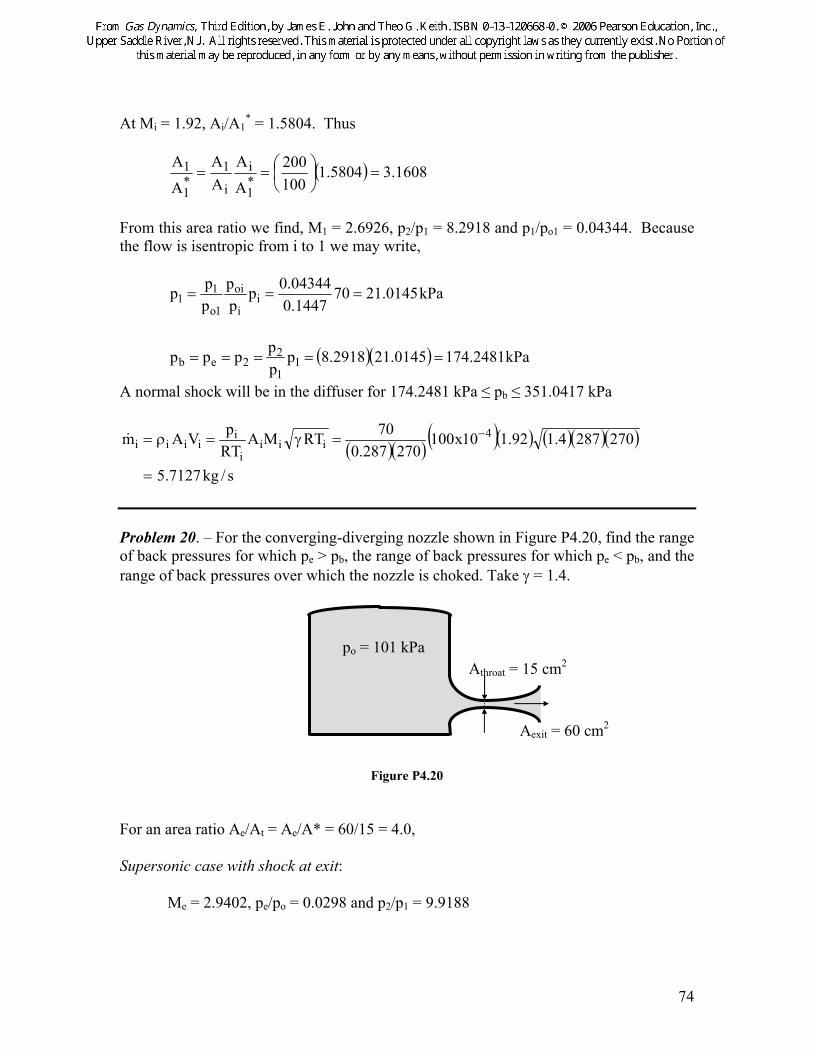
Problem 15. – Sketch p versus x for the case shown in Figure P3.15.

Figure P3.15

M > 1 M > 1

x

x

p

throat

44

Problem 16. – Steam is to be expanded to Mach 2.0 in a converging-diverging nozzle from an inlet velocity of 100 m/s. The inlet area is 50 cm2; inlet static temperature is 500 K. Assuming isentropic flow, determine the throat and exit areas required. Assume the steam to behave as a perfect gas with constant γ = 1.3.

( )

1826.06997.547

1005005.4613.1

100Mi ===

2throat* cm 3050.15

2669.350A ,2669.3

AA

===

For 2exit

t

e* cm 1389.27A so7732.1

AA

AA ,0.2M ====

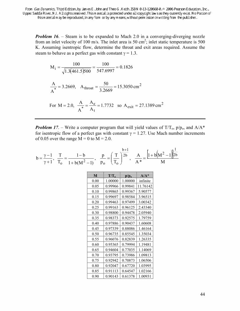
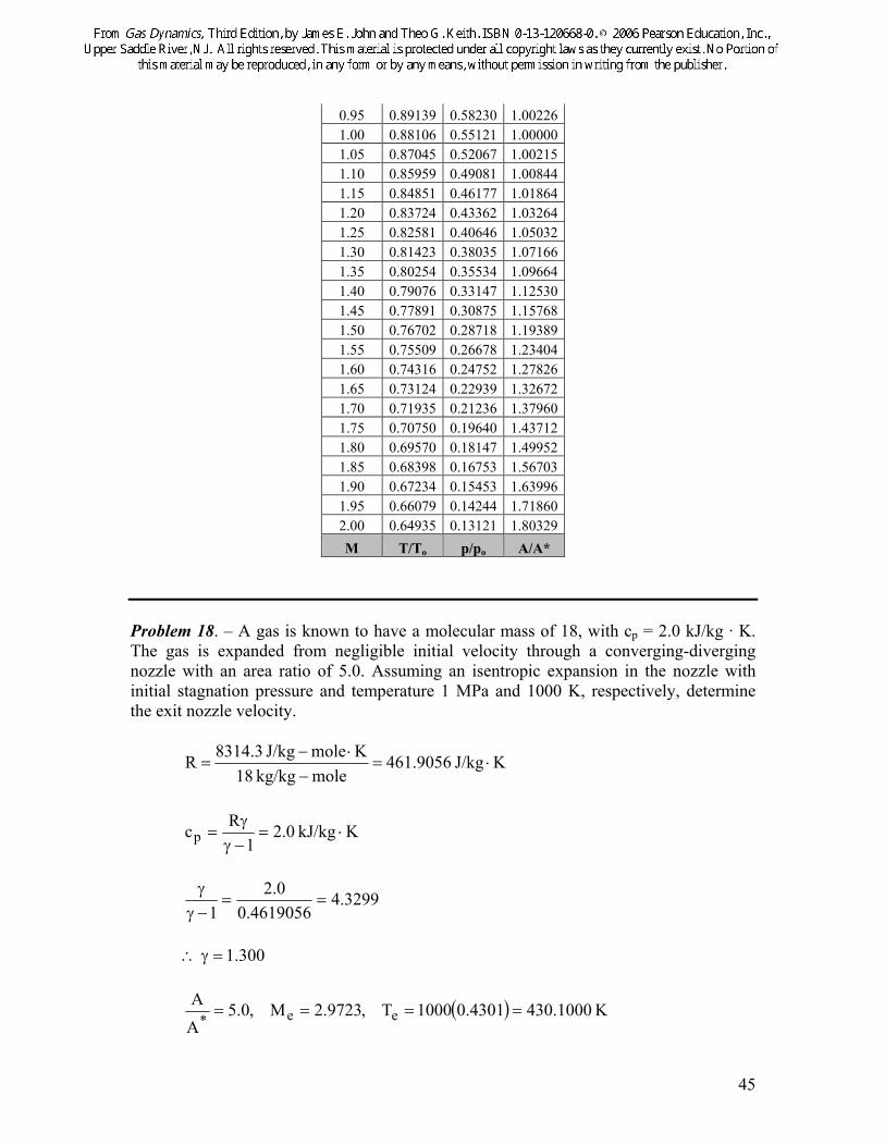
Problem 17. – Write a computer program that will yield values of T/To, p/po, and A/A* for isentropic flow of a perfect gas with constant γ = 1.27. Use Mach number increments of 0.05 over the range M = 0 to M = 2.0.

11b

+γ−γ

= , )1M(b1

b1TT

2o −+

−= ,

b21b

oo TT

pp

+

⎟⎟⎠

⎞⎜⎜⎝

⎛= , ( )[ ]

M1Mb1

*AA b2

12 −+

=

M T/To p/po A/A*

0.00 1.00000 1.00000 infinite 0.05 0.99966 0.99841 11.761420.10 0.99865 0.99367 5.905770.15 0.99697 0.98584 3.965150.20 0.99463 0.97499 3.003420.25 0.99163 0.96125 2.433400.30 0.98800 0.94478 2.059400.35 0.98373 0.92575 1.797590.40 0.97886 0.90437 1.606080.45 0.97339 0.88086 1.461640.50 0.96735 0.85545 1.350340.55 0.96076 0.82839 1.263350.60 0.95365 0.79994 1.194810.65 0.94604 0.77035 1.140690.70 0.93795 0.73986 1.098130.75 0.92942 0.70873 1.065060.80 0.92047 0.67720 1.039950.85 0.91113 0.64547 1.021660.90 0.90143 0.61378 1.00931

45

0.95 0.89139 0.58230 1.002261.00 0.88106 0.55121 1.000001.05 0.87045 0.52067 1.002151.10 0.85959 0.49081 1.008441.15 0.84851 0.46177 1.018641.20 0.83724 0.43362 1.032641.25 0.82581 0.40646 1.050321.30 0.81423 0.38035 1.071661.35 0.80254 0.35534 1.096641.40 0.79076 0.33147 1.125301.45 0.77891 0.30875 1.157681.50 0.76702 0.28718 1.193891.55 0.75509 0.26678 1.234041.60 0.74316 0.24752 1.278261.65 0.73124 0.22939 1.326721.70 0.71935 0.21236 1.379601.75 0.70750 0.19640 1.437121.80 0.69570 0.18147 1.499521.85 0.68398 0.16753 1.567031.90 0.67234 0.15453 1.639961.95 0.66079 0.14244 1.718602.00 0.64935 0.13121 1.80329M T/To p/po A/A*

Problem 18. – A gas is known to have a molecular mass of 18, with cp = 2.0 kJ/kg · K. The gas is expanded from negligible initial velocity through a converging-diverging nozzle with an area ratio of 5.0. Assuming an isentropic expansion in the nozzle with initial stagnation pressure and temperature 1 MPa and 1000 K, respectively, determine the exit nozzle velocity.

KJ/kg 9056.461molekg/kg 18

KmoleJ/kg 3.8314R ⋅=−

⋅−=

KkJ/kg 0.21

Rcp ⋅=−γγ

=

3299.44619056.0

0.21

==−γγ

∴ 300.1=γ

( ) K 1000.4304301.01000T ,9723.2M ,0.5AA

ee* ====

46

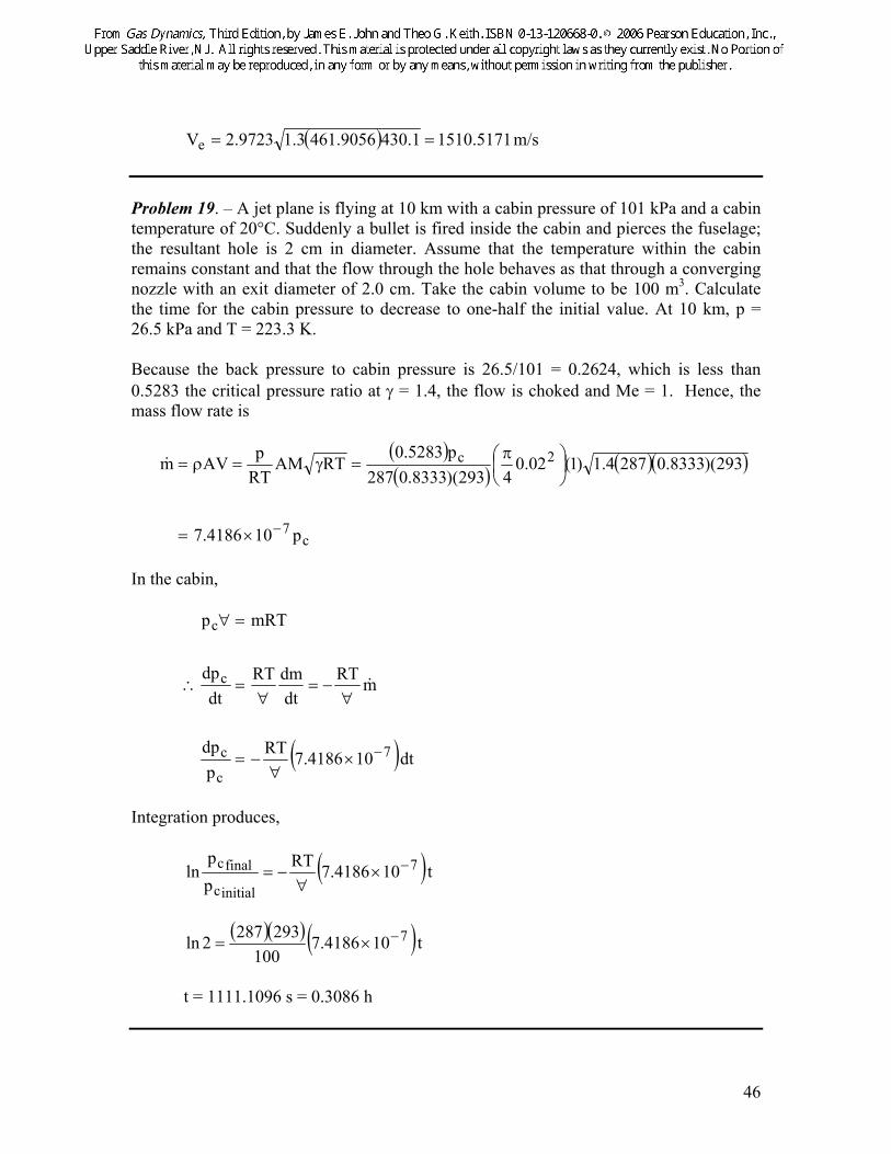
( ) m/s 5171.15101.4309056.4613.19723.2Ve == Problem 19. – A jet plane is flying at 10 km with a cabin pressure of 101 kPa and a cabin temperature of 20°C. Suddenly a bullet is fired inside the cabin and pierces the fuselage; the resultant hole is 2 cm in diameter. Assume that the temperature within the cabin remains constant and that the flow through the hole behaves as that through a converging nozzle with an exit diameter of 2.0 cm. Take the cabin volume to be 100 m3. Calculate the time for the cabin pressure to decrease to one-half the initial value. At 10 km, p = 26.5 kPa and T = 223.3 K.

Because the back pressure to cabin pressure is 26.5/101 = 0.2624, which is less than 0.5283 the critical pressure ratio at γ = 1.4, the flow is choked and Me = 1. Hence, the mass flow rate is

( )( ) ( )( )

p104186.7

293)(8333.02874.1)1(02.04293)(8333.0287

p5283.0RTAM

RTpAVm

c7

2c

−×=

⎟⎠⎞

⎜⎝⎛ π=γ=ρ=&

In the cabin,

( )dt 104186.7RTp

dp

mRTdtdmRT

dtdp

mRTp

7

c

c

c

c

−×∀

−=

∀−=

∀=∴

=∀

&

Integration produces,

( ) t104186.7RTpp

ln 7

initialc

finalc −×∀

−=

( )( ) ( ) t104186.7100

2932872ln 7−×=

t = 1111.1096 s = 0.3086 h

47

Problem 20. – A rocket nozzle is designed to operate isentropically at 20 km with a chamber pressure of 2.0 MPa and chamber temperature of 3000 K. If the products of combustion are assumed to behave as a perfect gas with constant specific heats (γ = 1.3 and MM = 20), determine the design thrust for a nozzle throat area of 0.25 m2. At 20 km, p = 5.53 kPa

o

e

r

bpp

002765.02000

53.5pp

===

( ) K 4000.77030002568.0TTTT ,3923.4M o

eoee ==⎟⎟

⎠

⎞⎜⎜⎝

⎛==

At design ( ) ApmVThrust eee +=

m/s 1293.28344.77020

3.83143.13923.4Ve =⎟⎠⎞

⎜⎝⎛=

Now at the throat M t = 1, so (p/po)t = 0.5457 and (T/To)t = 0.8696.

( )

( )( ) ( )

( )( )( )

s/kg7290.298

m/s 3805.1187m25.0kg/m 0063.1

m/s 3000)(8696.020

3.83143.1)1(m25.0K3000)(8696.0

KkgkNm

203143.8

kN/m 20005457.0m

23

22

t

=

=

⎟⎠⎞

⎜⎝⎛

⎥⎥⎥⎥

⎦

⎤

⎢⎢⎢⎢

⎣

⎡

⎟⎟⎠

⎞⎜⎜⎝

⎛⋅

=&

( )( ) ( )[ ]

0.8480MN 0.0014 8466.0

)000,000,1/()25.0(55301293.28347290.298Thrust

=+=

+=

Problem 21. – A converging nozzle has a rectangular cross section of a constant width of 10 cm. For ease of manufacture, the sidewalls of the nozzle are straight, making an angle of 10° with the horizontal, as shown in Figure P3.21. Determine and plot the variation of M, T, and p with x, taking M1 = 0.4, Po1 = 200 kPa, and To1 = 350 K. Assume the

48

working fluid to be air, which behaves as a perfect gas with constant specific heats (γ = 1.4), and that the flow is isentropic.

Figure P3.21 . A2 = A*

5901.1*A

A,4.0M ,cm 100A 11

21 ===

cm 289.6h so ,cm 89.62 5901.1100A 2

2 ===

( )10tan2hhx 1 −=

h (cm) x (cm) A/A* M p (kPa) T (K) 10.00 0 1.5901 0.400 179.1 339.2 9.50 1.418 1.5106 0.426 176.5 337.7 9.00 2.836 1.4311 0.457 173.3 336.0 8.50 4.253 1.3516 0.494 169.3 333.7 8.00 5.671 1.2721 0.539 164.1 330.8 7.50 7.089 1.1926 0.596 157.3 326.8 7.00 8.507 1.1131 0.676 147.3 320.7 6.50 9.925 1.0336 0.812 129.7 309.3 6.29 10.523 1.0000 1.000 105.7 291.7

10 cm

h

10 cm

Cross section at 2

10 cm

Cross section at 1

x

M2 = 1.0

M1 = 0.4 Po1 = 200kPa To1 = 350 K 2

10o

1

49

0.00.20.40.60.81.0

0.0 2.0 4.0 6.0 8.0 10.0 12.0

x

M

0

50

100

150

200

250

300

350

400

0.0 2.0 4.0 6.0 8.0 10.0 12.0

x

p(kP

a) a

nd T

(K)

Problem 22. – A spherical tank contains compressed air at 500 kPa; the volume of the tank is 20 m3. A 5-cm burst diaphragm in the side of the tank ruptures, causing air to escape from the tank. Find the time required for the tank pressure to drop to 200 kPa. Assume the temperature of the air in the tank remains constant at 280 K, the ambient pressure is 101 kPa and that the airflow through the opening can be treated as isentropic flow through a converging nozzle with a 5-cm exit diameter.

For ( ) so choked5283.0 505.0200101

pp

,Pak 200po

btank <===

( ) K 3240.2332808333.0T , p 5283.0p eoe ===

( ) m/s 1855.3063240.2330.2874.1RTV ee ==γ=

( ) 1855.306 05.043240.233287.0

p 5283.0m 2o ⎟⎠⎞

⎜⎝⎛ π=&

= 0.004743 po kg/s with po in kPa

50

In the tank,

po∀= mRT

( )oo p 004743.0RTmRT

dtdmRT

dtdp

∀−=

∀−=

∀= &

( ) ( )dt 004743.020

270287.0p

dp

o

o −=

t01838.0500200ln −=

( ) s 8526.4901838.0

4.0 lnt =−

=

Problem 23. – A converging-diverging nozzle has an area ratio of 3.3 to 1. The nozzle is supplied from a tank containing a gas at 100 kPa and 270 K (see Figure P3.23). Determine the maximum mass flow possible through the nozzle and the range of back pressures over which the mass flow can be attained assuming the gas is (a) helium (γ = 1.67, R = 2.077 kJ/kg·K) and (b) hydrogen (γ = 1.4, R = 4.124 kJ/kg·K).

Figure P3.23

(a) Helium: 3.3*A

A ,67.1 e ==γ

1494.3,1739.0Me =

Maximum pb to choke nozzle: at Me = 0.1739, 9752.0pp

eo=⎟⎟

⎠

⎞⎜⎜⎝

⎛

Maximum pb to choke nozzle = 97.52 kPa Nozzle choked for kPa52.97pb ≤

To = 270 K po = 100 kPa

Athroat = 60 cm2

51

throatthroatthroat

throatmax RTAM

RTpm γ=&

( )( ) ( ) ( )( )2707491.0207767.1)1(1060

2707491.0077.21004867.0 4−×=

kg/s 5822.0mmax =&

(b) Hydrogen: 3.3*A

A ,40.1 e ==γ

9780.0pp ,1787.0M

eoe =⎟⎟

⎠

⎞⎜⎜⎝

⎛=

Nozzle choked for all kPa8.97pb ≤

( )( ) ( ) ( )( )2708333.041244.1)1(1060

2708333.0124.41005283.0m 4

max−×=&

= 0.3894 kg/s

Problem 24. – Superheated steam is stored in a large tank at 6 MPa and 800°C. The steam is exhausted isentropically through a converging-diverging nozzle. Determine the velocity of the steam flow when the steam starts to condense, assuming the steam to behave as a perfect gas with γ = 1.3. Solution Using Steam Table Data At 6 MPa, 800°C: KkJ/kg 6554.7s1 ⋅=

1111 vpuh +=

( )( )kgkJ08159.06000

kgkJ2.3641 +=

= 4130.7 kJ/kg Steam will just condense for s2 = sg = s1

52

At 45 kPa, 6709.7s , kPa40at ;6307.7s gg == Interpolation gives

kgkJ8.2638h ,C77T Pa,k 42p 222 =°==

( ) ( ) m/s 172710008.26387.41302hh2V 212 =−=−=

Solution Assuming Steam is a Perfect Gas

K 873600273T ,7794.3M ,007.06000

42pp

eeo

=+====

T2 = 873 (0.3182) = 277.7886 K ( ) m/s 8994.15427886.2775.4613.17794.3V2 == Because the second answer assumes that the steam is a perfect gas with constant specific heats, the first answer is more accurate. Problem 25. – Air is stored in a tank 0.037661m3 in volume at an initial pressure of 5,760.6 kPa and a temperature of 321.4K. The gas is discharged through a converging nozzle with an exit area of 3.167x10-5 m2. For a back-pressure of 101 kPa, assuming a spatially lumped polytropic process in the tank, i.e., pvn = constant, and isentropic flow in the nozzle, i.e., pvγ = constant, compare predicted tank pressures to the measured values contained the following table. Try various values of the polytropic exponent, n, from 1.0 (isothermal) to 1.4 (isentropic). Perform only a Stage I analysis, i.e., the nozzle is choked.

time, sec 0.0 1.0 2.0 3.0 4.0 5.0 6.0 7.0 9.0 11.0 13.0 15.0 17.0 19.0

po/po1 1.000 0.717 0.551 0.448 0.358 0.281 0.241 0.199 0.142 0.104 0.078 0.059 0.044 0.033

Now from the continuity equation

eeee VAmdtdm

ρ−=−= &

For polytropic expansion within the tank

53

n1o

1ono

o ppρ

=ρ

So

n1

1o

o1oo p

p⎟⎟⎠

⎞⎜⎜⎝

⎛ρ=ρ

And for isentropic expansion in the nozzle

γγ ρ=

ρ e

e

o

o pp

So

γ⎟⎟⎠

⎞⎜⎜⎝

⎛ρ=ρ

1

1o

ooe p

p

For a choked flow: Me = 1, Ve = ae = √γpe/ρe and

)1/()1/(2e

e

o2

1M2

11pp −γγ−γγ

⎟⎠⎞

⎜⎝⎛ +γ

=⎟⎠⎞

⎜⎝⎛ −γ+=

So,

)1/(

oe 21pp

γ−γ

⎟⎠⎞

⎜⎝⎛ +γ

=

Therefore,

n1

1o

o11

1oe pp

21

⎟⎟⎠

⎞⎜⎜⎝

⎛⎟⎠⎞

⎜⎝⎛ +γ

ρ=ρ γ−

Now,

( ) ( ) n21

1o

o121

211o

121o

21oe

eeee

eeeeeeeeee

pp

21

21pA

pApAaAVAm

⎟⎟⎠

⎞⎜⎜⎝

⎛⎟⎠⎞

⎜⎝⎛ +γ

ρ⎟⎠⎞

⎜⎝⎛ +γ

ργ=

ργ=ρ

γρ=ρ=ρ=

γ−γ−γ

&

54

Using ao1 = √γpo1/ρ01 the mass flow rate at the exit can be written as

( ) n21n

on2

1

1o

121

211o

1o1oee p

p1

21

paAm

+γ−

+γ

⎟⎟⎠

⎞⎜⎜⎝

⎛⎟⎠⎞

⎜⎝⎛ +γρ

=&

Now the time rate of change of the mass within the tank is given by

( )

dtdp

ppndt

ddtdm on

n1

on11o

1oo−

⎥⎥

⎦

⎤

⎢⎢

⎣

⎡ ∀ρ=

ρ∀=

Equating this to the exiting flow rate gives

( )( ) n2

1n

on2

1

1o

121

211o

1o1oee

onn1

on11o

1o pp1

21

paAm

dtdp

ppn

+γ−

+γ−

⎟⎟⎠

⎞⎜⎜⎝

⎛⎟⎠⎞

⎜⎝⎛ +γρ

−=−=⎥⎥

⎦

⎤

⎢⎢

⎣

⎡ ∀ρ&

or

( )

( ) n2n1

1o12

11oe

n2121n11o

121

1oeon2n31

oon2

1nnn1

oo

n21n

o

nn1

o

p2

1anA

p2

1anAdt

dpp

dtdp

pdt

dp

p

p

−γ−

+γ

−−γ−+γ−⎟

⎠⎞

⎜⎝⎛ +

−⎟⎠⎞

⎜⎝⎛ −

+

−

⎟⎠⎞

⎜⎝⎛ +γ

∀−

=

⎟⎠⎞

⎜⎝⎛ +γ

∀−

===

Integration yields, (note: n2n11

n2n31 −

=+− )

( ) tp2

1aA2

1npp n2n1

1o12

11oen2

n1

1on2n1

o

−γ−

+γ−−

⎟⎠⎞

⎜⎝⎛ +γ⎟⎟⎠

⎞⎜⎜⎝

⎛∀

⎟⎠⎞

⎜⎝⎛ −

=−

Rearrangement brings

55

( )n1n2

121

1oe

1o

o t2

1aA2

1n1p

p−

γ−+γ

⎥⎥⎥

⎦

⎤

⎢⎢⎢

⎣

⎡

⎟⎠⎞

⎜⎝⎛ +γ⎟⎟⎠

⎞⎜⎜⎝

⎛∀

⎟⎠⎞

⎜⎝⎛ −

+=

Note this is not valid for n =1, the isothermal case which must be treated separately. For n = 1

( )o

121

1o

1o1oee p

21

paAm γ−

+γ

⎟⎠⎞

⎜⎝⎛ +γρ

=&

⎟⎟⎠

⎞⎜⎜⎝

⎛ρ=ρ

1o

o1oo p

p

( )o

121

1o

1o1oee

o

1o

1oo p2

1p

aAmdt

dppdt

ddtdm γ−

+γ

⎟⎠⎞

⎜⎝⎛ +γρ

−=−=ρ

∀=ρ

∀= &

Canceling, separating variables, integrating and rearranging yields,

( ) t121

211oaeA

1o

o epp

γ−+γ

⎟⎠⎞

⎜⎝⎛ +γ

∀−

=

A spreadsheet program was written and run for various n. A table of the results is as follows

n = 1.0 1.1 1.2 1.3 1.4 t po/po1 po/po1 po/po1 po/po1 po/po1 po/po1 (exp)

0.0 1.0000 1.0000 1.0000 1.0000 1.0000 1.000 1.0 0.8396 0.8257 0.8122 0.7990 0.7862 0.717 2.0 0.7049 0.6830 0.6620 0.6421 0.6230 0.551 3.0 0.5918 0.5658 0.5415 0.5187 0.4974 0.448 4.0 0.4969 0.4695 0.4443 0.4212 0.3999 0.358 5.0 0.4172 0.3902 0.3658 0.3437 0.3237 0.281 6.0 0.3503 0.3247 0.3021 0.2818 0.2636 0.241 7.0 0.2941 0.2707 0.2502 0.2321 0.2159 0.199 9.0 0.2073 0.1890 0.1731 0.1594 0.1473 0.142

11.0 0.1461 0.1327 0.1211 0.1112 0.1025 0.104 13.0 0.1030 0.0937 0.0856 0.0787 0.0726 0.078 15.0 0.0726 0.0665 0.0611 0.0564 0.0522 0.059 17.0 0.0512 0.0474 0.0440 0.0410 0.0382 0.044 19.0 0.0361 0.0340 0.0320 0.0301 0.0283 0.033

56

CChhaapptteerr FFoouurr

SSTTAATTIIOONNAARRYY NNOORRMMAALL SSHHOOCCKK WWAAVVEESS

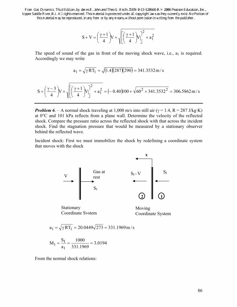
Problem 1. – A helium flow with a velocity of 2500 m/s and static temperature of 300 K undergoes a normal shock. Determine the helium velocity and the static and stagnation temperatures after the wave. Assume the helium to behave as a perfect gas with constant γ = 5/3 and R = 2077 J/kg·K.

( )( )

4153.14219.1766

250030020773/5

2500M1 ==

From the normal shock relations

( ) K3800.3792646.1300T ,2646.1TT

21

2 ===

From the isentropic relations

K 1681.420714.0

300TT,7140.0TT

1oo21o

1 ====

From the normal shock relations

m/s 7067.14567162.1

2500V ,7162.1VV

22

1

1

2 ====ρρ

Problem 2. – A normal shock occurs at the inlet to a supersonic diffuser, as shown in Figure P4.2. Ae/Ai is equal to 3.0. Find Me, pe, and the loss in stagnation pressure (poi – poe). Repeat for a shock at the exit. Assume γ = 1.4.

57

Figure P4.2 Shock at inlet:

05853.0pp,

*A*A4990.0

pp,5.2MM

1o

1

2

1

1o

2o1 =====∞

( )( )( ) 9471.34990.06367.20.3AA

AA

AA

AA

AA

*2

*1

*1

1

1

e*2

e*e

e ==⎟⎟⎠

⎞⎜⎜⎝

⎛⎟⎟⎠

⎞⎜⎜⎝

⎛⎟⎟⎠

⎞⎜⎜⎝

⎛==

Me = 0.1486

( ) kPa2554.858526.1704990.0p, kPa8526.17005853.010p

,4990.0pp,9847.0

pp

2o1o

1o

2o

2o

e

====

==

( ) kPa 9510.832554.859847.0pppp 2o

2o

ee ===

( ) kPa 5972.854990.018526.170pp1pp-p

o1

o2o1eoio =−=⎟⎟

⎠

⎞⎜⎜⎝

⎛−=

Shock at exit:

( ) 9101.76367.23*A

A,6367.2*A

A,0.3AA

1

1

1

i

i

1 ====

4451.0M ,6649.3M 21 ==

( )( ) kPa5482.271005853.0

101040.05038.15ppp

pp

pp p i

i

o1

1o

1

1

22 =⎟

⎠⎞

⎜⎝⎛==

e

M∞ = 2.5 p∞ = 10 kPa

i

1 2

e

M∞ = 2.5 p∞ = 10 kPa

i

1 2

58

( ) kPa2961.1391847.018526.170pp1ppp

o1

2ooiboio =−=⎟⎟

⎠

⎞⎜⎜⎝

⎛−=−

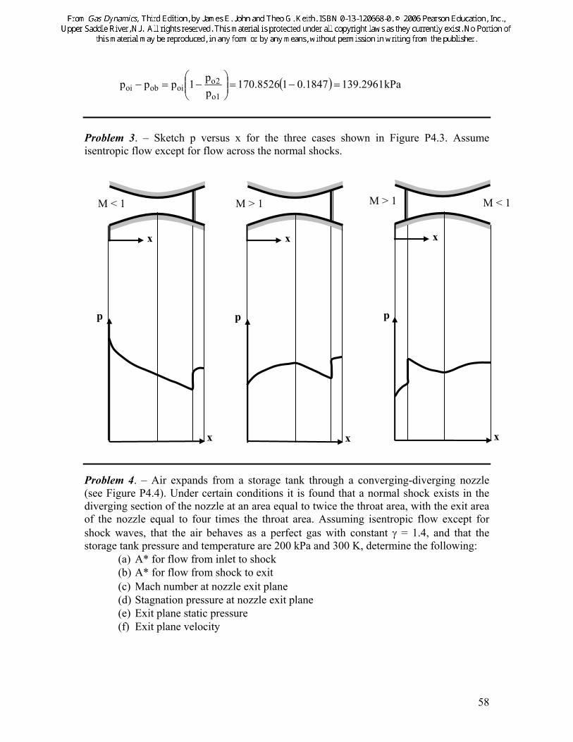
Problem 3. – Sketch p versus x for the three cases shown in Figure P4.3. Assume isentropic flow except for flow across the normal shocks.

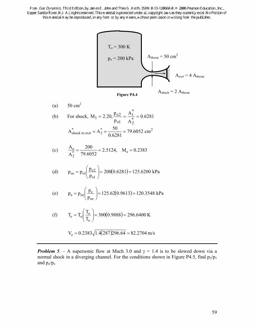
Problem 4. – Air expands from a storage tank through a converging-diverging nozzle (see Figure P4.4). Under certain conditions it is found that a normal shock exists in the diverging section of the nozzle at an area equal to twice the throat area, with the exit area of the nozzle equal to four times the throat area. Assuming isentropic flow except for shock waves, that the air behaves as a perfect gas with constant γ = 1.4, and that the storage tank pressure and temperature are 200 kPa and 300 K, determine the following:

(a) A* for flow from inlet to shock (b) A* for flow from shock to exit (c) Mach number at nozzle exit plane (d) Stagnation pressure at nozzle exit plane (e) Exit plane static pressure (f) Exit plane velocity

M < 1

x

M > 1

x

M < 1 M > 1

x

x

p

x

p

x

p

59

Figure P4.4 (a) 50 cm2

(b) For shock, 6281.0A

App

,20.2M*2

*1

1o

2o1 ===

2*2

*xitshock to e cm6052.79

6281.050AA ===

(c) 2383.0M ,5124.26052.79

200AA

e*2

e ===

(d) ( ) kPa6200.1256281.0200pppp

1o

2o1ooe ==⎟⎟

⎠

⎞⎜⎜⎝

⎛=

(e) ( ) kPa3548.1209613.062.125ppppoe

eoee ==⎟⎟

⎠

⎞⎜⎜⎝

⎛=

(f) ( ) K 6400.2969888.0300TTTT

o

eoe ==⎟⎟

⎠

⎞⎜⎜⎝

⎛=

( ) m/s 2704.8264.2962874.12383.0Ve ==

Problem 5. – A supersonic flow at Mach 3.0 and γ = 1.4 is to be slowed down via a normal shock in a diverging channel. For the conditions shown in Figure P4.5, find p2/p1 and pe/pi.

To = 300 K po = 200 kPa Athroat = 50 cm2

Aexit = 4 Athroat

Ashock = 2 Athroat

60

Figure P4.5 From the isentropic Mach number-area relation at the inlet and exit Mach numbers, we have

50.0AA

ninformatiogiventhefromand,5901.1A

A,2346.4

A

A

e

i*e

e*i

i ===

Hence,

( )( )1o

2o

oi

oe*e

e

e

i

i

*i

*e

*i

pp

pp1878.05901.150.0

2346.41

AA

AA

AA

AA

===⎟⎠⎞

⎜⎝⎛==

Now using this ratio of stagnation pressures across the shock, we can find the Mach number on the upstream side of the shock, i.e., M1, and in turn, determine the pressure ratio across the shock: M1 = 3.6455

3378.15pp

1

2 =

( )( ) 1790.602722.0

11878.08956.0pp

pp

pp

pp

i

oi

io

oe

oe

e

i

e =⎟⎠⎞

⎜⎝⎛==

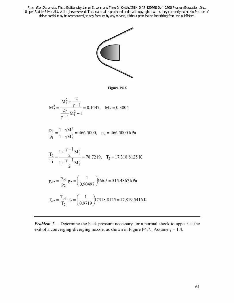
Problem 6. – A body is reentering the earth's atmosphere at a Mach number of 20. In front of the body is a shock wave, as shown in Figure P4. 7. Opposite the nose of the body, the shock can be seen to be normal to the flow direction. Determine the stagnation pressure and temperature to which the nose is subjected. Assume that the air behaves as a perfect gas (neglect dissociation) with constant γ = 1.4. The ambient pressure and temperature are equal to 1.0 kPa and 220 K.

Mi = 3.0

Ai

2 1

ie A2A =

e

i Me = 0.4

Inlet Exit

61

Figure P4.6

3804.0M ,1447.01M

12

12M

M 221

21

22 ==

−−γγ

−γ+

=

kPa5000.466p ,5000.466M1M1

pp

222

21

1

2 ==γ+γ+

=

K8125.318,17T ,7219.78M

211

M2

11

TT

222

21

1

2 ==−γ

+

−γ+

=

Pak 4867.5155.46690497.0

1pppp 2

2

2o2o =⎟

⎠⎞

⎜⎝⎛==

K 5416.819,178125.173189719.01T

TTT 2

2

2o2o =⎟

⎠⎞

⎜⎝⎛==

Problem 7. – Determine the back pressure necessary for a normal shock to appear at the exit of a converging-diverging nozzle, as shown in Figure P4.7. Assume γ = 1.4.

62

Figure P4.7

From the given area ratio, we use the Newton-Raphson method to determine the supersonic Mach number on the upstream side of the shock. Then we may use the isentropic and shock relations to determine the pressure ratios that enable us to compute the back pressure:

4656.5pp ,09393.

pp,1972.2M

1

2

1o

11 ===

( )( )( )( ) kPa38.513 MPa51338.00.109393.04656.511ppp

pp

pp

ppp 1o

1o

1

1

2

2

e

e

bb ====

Problem 8. – A normal shock is found to occur in the diverging portion of a converging-diverging nozzle at an area equal to 1.1 times the throat area. If the nozzle has a ratio of exit area to throat area of 2.2, determine the percent of decrease in nozzle exit velocity due to the presence of the shock (compared with the exit velocity of a perfectly expanded isentropic supersonic nozzle flow). Assume the flow is expanded from negligible velocity, that the stagnation temperature of the flow is the same for both cases, and that the working fluid is steam, which behaves as a perfect gas with constant γ = 1.3. With no shock, From the given area ratio and because the flow is choked: Ae/At = Ae/A* = 2.2, we can determine the exit Mach number using the Newton-Raphson method and find that Me = 2.2201, and therefore, the static to total temperature ratio is 0.5749. Hence,

( )5749.0RT2201.2RTMV oeee γ=γ= With shock,

3598.1M find Raphson we-Newton using so ,1.1AA

AA

1*1

1*1

s ===

pr = 1.0 MPa Tr = 800 K

0.2AA

throat

exit =

pb

63

9662.0AA

pp

*2

*1

1o

2o ==

( )( )( ) 1256.29662.012.2AA

AA

AA

AA

*2

*1

*1

t

t

e*2

e ===

From this area ratio we are able to extract the exit Mach number again using the Newton-Raphson method, therefore, the static to total temperature ratio

9876.0TT ,2888.0M

o

ee ==

( )9876.0RT2888.0V oe γ=

( ) ( )

( )

decrease 82.9502% 6833.12870.01100

5749.0RT2201.29876.0RT2888.05749.0RT2201.2

100Vindecrease %o

ooe

=⎟⎠⎞

⎜⎝⎛ −=

⎟⎟⎠

⎞⎜⎜⎝

⎛

γγ−γ

=

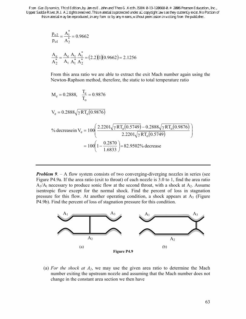
Problem 9. – A flow system consists of two converging-diverging nozzles in series (see Figure P4.9a. If the area ratio (exit to throat) of each nozzle is 3.0 to 1, find the area ratio A3/Al necessary to produce sonic flow at the second throat, with a shock at A2. Assume isentropic flow except for the normal shock. Find the percent of loss in stagnation pressure for this flow. At another operating condition, a shock appears at A3 (Figure P4.9b). Find the percent of loss of stagnation pressure for this condition.

(a) (b)

Figure P4.9

(a) For the shock at A2, we may use the given area ratio to determine the Mach number exiting the upstream nozzle and assuming that the Mach number does not change in the constant area section we then have

A1 A3

A2

A1 A3

A2

64

2411.2AAso,4462.0

AA

pp,6374.2M *

1

*2

*2

*1

1o

2o1 ====

Since sonic flow exists at both A1 and A3, we have, 2411.2AA

AA

*1

*2

1

3 ==

% loss in stagnation pressure = ( ) %3800.551004462.01100p

pp

1o

2o1o =−=⎟⎟⎠

⎞⎜⎜⎝

⎛ −

(b) For shock at A3, we have from part (a) A3/A1 = A3/A* = 2.411. Using this area

ratio, we can find the Mach number on the upstream side of the shock, i.e.,

3238.2M1 = And so,

5728.0pp

1o

2o =

or 42.72% loss of stagnation pressure

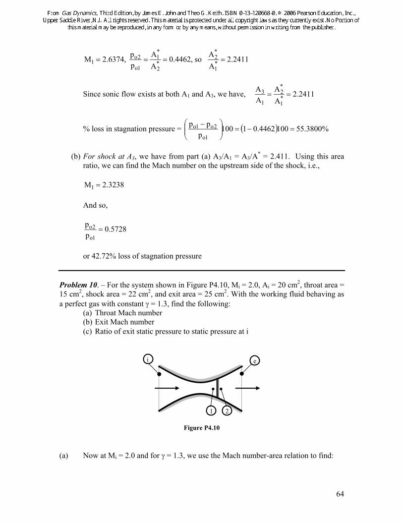
Problem 10. – For the system shown in Figure P4.10, Mi = 2.0, Ai = 20 cm2, throat area = 15 cm2, shock area = 22 cm2, and exit area = 25 cm2. With the working fluid behaving as a perfect gas with constant γ = 1.3, find the following:

(a) Throat Mach number (b) Exit Mach number (c) Ratio of exit static pressure to static pressure at i

Figure P4.10 (a) Now at Mi = 2.0 and for γ = 1.3, we use the Mach number-area relation to find:

1 2

e i

65

7732.1AA

*1

i = .

Hence,

( ) 3299.17732.12015

AA

AA

AA

*1

i

i

t*1

t ===

From which we determine the result of part (a),

6620.1Mt =

(b) 9505.13299.11522

AA

AA

AA

*1

t

t

s*1

s === ; therefore from the Newton-Raphson method

we find:

0995.2M1 = At this Mach number we can compute the total pressure ratio across the shock

*2

*1

1o

2o

AA6502.0

pp

==

Thus,

( ) 4412.1)6502.0(3299.11525

AA

AA

AA

AA

*2

*1

*1

t

t

e*2

e ===

Me = 0.4571

(c) From the various Mach numbers computed thus far, we may determine the following pressure ratios and form the string,

3591.41305.01)6502.0)(1)(8749.0(

pp

pp

pp

pp

pp

i

1o

1o

2o

2o

oe

oe

e

a

e =⎟⎠⎞

⎜⎝⎛==

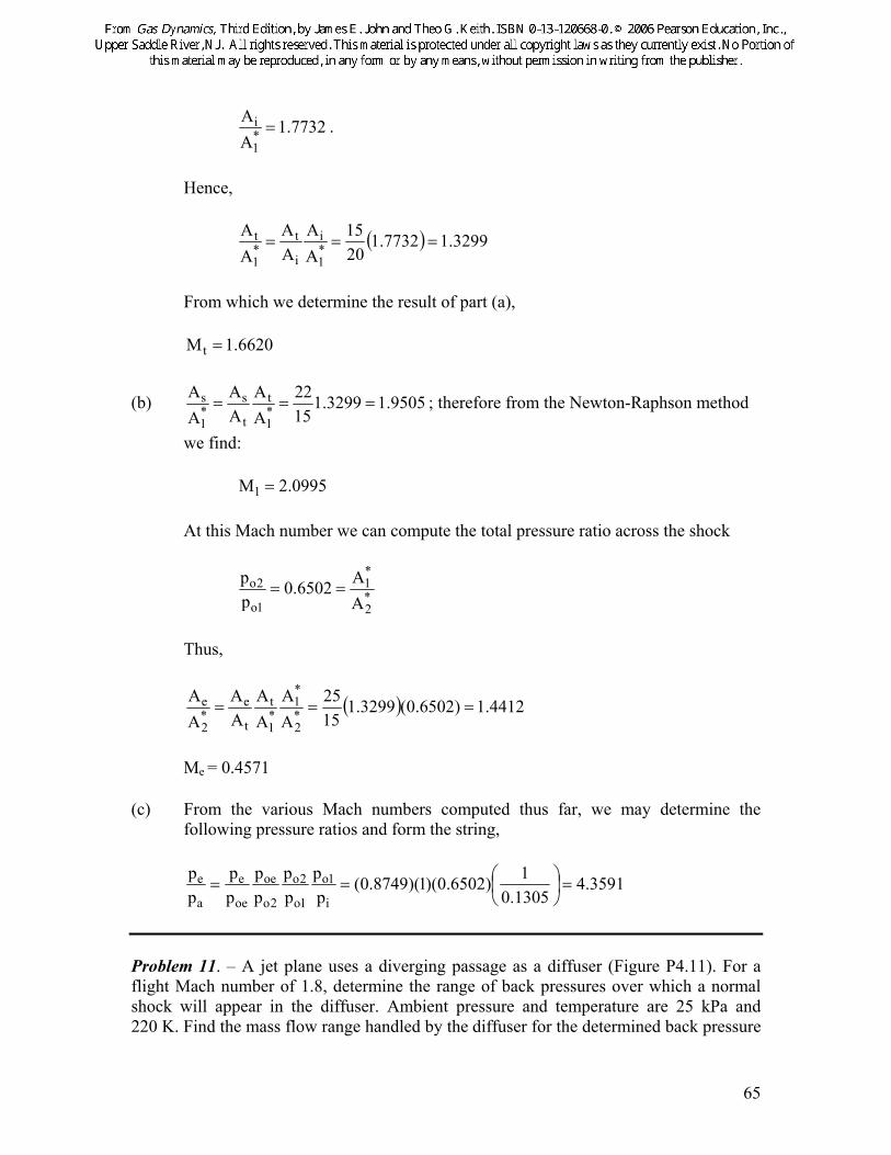
Problem 11. – A jet plane uses a diverging passage as a diffuser (Figure P4.11). For a flight Mach number of 1.8, determine the range of back pressures over which a normal shock will appear in the diffuser. Ambient pressure and temperature are 25 kPa and 220 K. Find the mass flow range handled by the diffuser for the determined back pressure

66

range. Also, the inlet and exit area are Ai = 250 cm2, Ae = 500 cm2. Assume isentropic flow except for the shocks. Take γ = 1.4.

Figure P4.11 For a shock at the inlet, with M1 = 1.8 and γ = 1.4, from the normal shock relations

*2

*1

1o

2o

AA8127.0

pp

==

( )( ) 3390.28127.04390.1250500

AA

AA

AA

AA

*2

*1

*1

i

i

e*2

e =⎟⎠⎞

⎜⎝⎛==

From this area ratio, we can determine the exit Mach number and therefore the exit static to total pressure ratio

9550.0pp,2574.0Mo2

ee ==

The following pressure ratio string may be readily formed

( )( ) ( ) kPa5127.111251740.018127.09550.0p

pp

pp

ppp i

i

1o

1o

2o

o2

ee ===

Next the mass flow rate is computed

( ) ( ) ( )( )

( )( )( )

s/kg2974.5

m/s 1664.535m0250.0kg/m 3959.0

2202874.18.110250220287.0

25AVRTpm

23

4

=

=

×== −&

M = 1.8 p = 25 kPa

pb

Ae Ai

67

For a shock at the exit,

( ) 8780.24390.1250500

AA

AA

AA

*i

i

i

e*1

1 ===

6799.7pp,0506.0

pp,5934.2M

1

2

1o

11 ===

( )( ) ( ) Pak 8338.55251740.010506.06799.7p

pp

pp

ppp 1o

1o

1

1

2e =⎟

⎠⎞

⎜⎝⎛== ∞

∞

The diffuser is choked so it passes the same mass flow for the back pressure range,

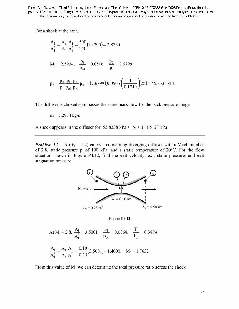
kg/s 5.2974m =& A shock appears in the diffuser for: 55.8338 kPa < pb < 111.5127 kPa Problem 12. – Air (γ = 1.4) enters a converging-diverging diffuser with a Mach number of 2.8, static pressure pi of 100 kPa, and a static temperature of 20°C. For the flow situation shown in Figure P4.12, find the exit velocity, exit static pressure, and exit stagnation pressure.

Figure P4.12

At Mi = 2.8, 3894.0TT,0368.0

pp,5001.3

AA

1o

i

1o

i*1

i ===

( ) 7632.1M ,4000.15001.325.010.0

AA

AA

AA

1*1

i

i

t*1

1 ====

From this value of M1 we can determine the total pressure ratio across the shock

1 2 e i

Ae = 0.50 m2

At = 0.10 m2

Ai = 0.25 m2

Mi = 2.8

68

*2

*1

1o

2o

AA8289.0

pp

==

( )( ) 8025.58289.05001.325.05.0

AA

AA

AA

AA

*2

*1

*1

i

i

e*2

e ===

From this area ratio we can compute the exit Mach number Me = 0.1003

9980.0TT ,9930.0

pp

o

e

2o

e ==

kPa 3913.27170368.0100p ,K 4397.752

3894.0293T oio ====

( ) kPa4457.22523913.27178289.0p eo == ( ) kPa6785.22364457.22529930.0pe == ( )( )( ) m/s 0943.559348.7502874.11003.0RTMV eee ==γ= Problem 13. – Write a computer program that will yield values of p2/p1, ρ2/ρ1, T2/T1, and po2/po1 for a fixed normal shock with a working fluid consisting of a perfect gas with constant γ = 1.20. Use Mach number increments of 0.05 over the range M = 1.0 to M = 2.5.

Let 11b

+γ−γ

= . Then,

( ) bM1bpp 2

11

2 −+=

( )b1bM

M21

21

1

2

−+=

ρρ

( )[ ]( )[ ]21

21

21

1

2

M

bM1bb1bMTT −+−+

=

69

( ) ( )b2b1

21

b21b

21

21

1o

2o

bM1b1

b1bM

Mpp

−+

⎥⎥⎦

⎤

⎢⎢⎣

⎡

−+⎥⎥⎦

⎤

⎢⎢⎣

⎡

−+=

M1 p2/p1 ρ2/ρ1 T2/T1 po2/po1 1.00 1.0000 1.0000 1.0000 1.0000 1.05 1.1118 1.0923 1.0178 0.9998 1.10 1.2291 1.1873 1.0352 0.9989 1.15 1.3518 1.2848 1.0521 0.9965 1.20 1.4800 1.3846 1.0689 0.9924 1.25 1.6136 1.4865 1.0855 0.9861 1.30 1.7527 1.5902 1.1022 0.9777 1.35 1.8973 1.6957 1.1189 0.9671 1.40 2.0473 1.8027 1.1357 0.9542 1.45 2.2027 1.9110 1.1527 0.9391 1.50 2.3636 2.0204 1.1699 0.9220 1.55 2.5300 2.1308 1.1873 0.9030 1.60 2.7018 2.2420 1.2051 0.8822 1.65 2.8791 2.3539 1.2231 0.8599 1.70 3.0618 2.4663 1.2415 0.8362 1.75 3.2500 2.5789 1.2602 0.8114 1.80 3.4436 2.6918 1.2793 0.7856 1.85 3.6427 2.8048 1.2987 0.7591 1.90 3.8473 2.9177 1.3186 0.7320 1.95 4.0573 3.0304 1.3388 0.7045 2.00 4.2727 3.1429 1.3595 0.6767 2.05 4.4936 3.2549 1.3806 0.6490 2.10 4.7200 3.3664 1.4021 0.6213 2.15 4.9518 3.4773 1.4240 0.5938 2.20 5.1891 3.5876 1.4464 0.5667 2.25 5.4318 3.6971 1.4692 0.5401 2.30 5.6800 3.8058 1.4925 0.5139 2.35 5.9336 3.9135 1.5162 0.4884 2.40 6.1927 4.0203 1.5404 0.4636 2.45 6.4573 4.1261 1.5650 0.4395 2.50 6.7273 4.2308 1.5901 0.4162 M1 p2/p1 ρ2/ρ1 T2/T1 po2/po1

Problem 14. – A converging-diverging nozzle has an area ratio (exit to throat) of 3.0. The nozzle is supplied from an air (γ = 1.4, R = 287 J/kg·K) reservoir in which the pressure and temperature are maintained at 270 kPa and 35°C, respectively. The nozzle is

70

exhausted to a back pressure of 101 kPa. Find the nozzle exit velocity and nozzle exit-plane static pressure. Since, pb/po = 101/270 = 0.3741 < 0.5283, the nozzle is choked. Hence the At = A*. So, for Ae/A* = 3.0 determine the subsonic and supersonic solutions, i.e., curves 4 and 5 in Fig. 4.14. This yields Me = 0.1974 and Me = 2.6374. For the subsonic solution: pe/po = 0.9732. Thus, pe = (0.9732)(270) = 262.7640 kPa, which is much larger than the given back pressure. For the supersonic solution: pe/po = 0.04730. Thus, pe = (0.0473)(270) = 12.7764 kPa, which is far lower than the given back pressure. The actual situation is somewhere in between these. For a shock in the exit of the nozzle (curve c in Fig 4.14), we use the shock relations at Me = M1 =2.6374 and find p2/p1 = 7.9486. Since p1 = 12.7764 kPa, p2 = pe = (12.7764)(7.9486) = 101.5545 kPa. Since this is larger than the given back pressure, this situation is also not possible. The actual case corresponds to curve d in Fig 4.14, where oblique shock waves (refer to Fig. 4.16) occur outside the nozzle in order to compress the exiting flow to the correct pressure. Thus, for pb = 101 kPa, pe = 12.7764 kPa and

( ) s/m9960.599308)4182.0(2874.16374.2RTMV eee ==γ= Problem 15. – A supersonic nozzle possessing an area ratio (exit to throat) of 3.0 is supplied from a large reservoir and is allowed to exhaust to atmospheric pressure (101 kPa). Determine the range of reservoir pressures over which a normal shock will appear in the nozzle. For what value of reservoir pressure will the nozzle be perfectly expanded, with supersonic flow at the exit plane? Find the minimum reservoir pressure to produce sonic flow at the nozzle throat. Assume isentropic flow except for shocks, with γ = 1.4. At Ae/A* = 3.0, Me = 0.1974 and pe/po = 0.9732 or Me = 2.6374 and pe/po = 0.0473.

For a shock just past the throat: kPa7813.1039732.0101pp or ===

For a shock at exit: ( )( ) kPa6393.2689486.70473.0

101pp or ===

Thus, for a shock in the nozzle: kPa6393.268pkPa7813.103 r ≤≤

71

For perfect isentropic expansion: ( ) kPa3066.21350473.0101pp or ===

Minimum reservoir pressure for sonic flow at nozzle throat: 103.7813 kPa Problem 16. – A converging-diverging nozzle with an area ratio (exit to throat) of 3.0 exhausts air (γ = 1.4) from a large high-pressure reservoir to a region of back pressure pb. Under a certain operating condition, a normal shock is observed in the nozzle at an area equal to 2.2 times the throat area. What percent of decrease in back pressure would be necessary to rid the nozzle of the normal shock? For As/A* = 2.2 , Ms = M1 = 2.3034. At this Mach number from the shock tables we find:

5818.0AA

pp

*2

*1

1o

2o ==

( )( )( ) 7454.15818.010.3AA

AA

AA

AA

*2

*1

*1

t

t

e*2

e ===

From this area ratio we find, Me = 0.3577 from which pe/po2 = 0.9154. Thus,

( )( ) 5326.05818.09154.0pp

pp

pp

pp

1o

2o

2o

e

1o

e

r

e ====

Now for a shock at the exit, i.e., As/A* = Ae/At = 3.0: M1 = = 2.6374 and in turn Me = 0.5005.

( )( )( ) 3760.09485.710473.0pp

pp

pp

pp

pp

1

2

2

e

1o

1

1o

e

r

e ====

% reduction = %4097.291005326.0

3760.05326.0=

−

Problem 17. – Due to variations in fuel flow rate, it is found that the stagnation pressure at the inlet to a jet-engine nozzle varies with time according to:

po = 200[1 + 0.1 sin (π/4)t], with t in seconds and po in kilopascals. Determine the resultant variation in nozzle flow rate, nozzle exhaust velocity, and exit-plane static pressure. The nozzle area ratio (exit to

72

throat) is 2.0 to 1, and the inlet stagnation temperature is 600 K. Assume negligible inlet velocity. The nozzle exhausts to an ambient pressure of 30 kPa; γ = 1.4; nozzle exit area is 0.3 m2; R = 0.3 kJ/kg · K.

( )( )( )( ) ( )( )( )( )

⎟⎠⎞

⎜⎝⎛ π

+==

⎟⎠⎞

⎜⎝⎛=

⎟⎟⎠

⎞⎜⎜⎝

⎛γ

⎟⎟⎠

⎞⎜⎜⎝

⎛⎟⎟⎠

⎞⎜⎜⎝

⎛

⎟⎟⎠

⎞⎜⎜⎝

⎛

=γ=ρ=

t4

sin8420.44200.48p2421.0

6008333.03004.10.10.23.0

6008333.03.0p5283.0

TTTRM

AAA

TTTR

ppp

RTMARTpVAm

o

o

oto

t

t

e

e

oto

oto

tttt

ttttth&

Hence, the stagnation pressure varies from 48.4200 − 4.8420 = 43.5780 kg/s to 48.4200 + 4.8420 = 53.2620 kg/s. The stagnation pressure varies from 200 – 20 = 180 kPa to 200 + 20 = 220 kPa. For a shock at the exit, for Ae/A* = 2.0, we find Me = M1 = 2.1972. From which we obtain and (p1/po1) = 0.0939 and (p2/p1) = 5.4656. Thus,

( )( ) kPa4545.584656.50939.0

30pp or ===

Hence, the exit velocity is constant,

( )( )( )( ) s/m7621.7866005088.03004.11972.2TTTRMV o

eoee ==⎟⎟

⎠

⎞⎜⎜⎝

⎛γ=

( ) ⎟⎠⎞

⎜⎝⎛ π

+== t4

sin8780.17800.18p0939.0p oe

Problem 18. – Helium enters a converging-diverging nozzle with a negligible velocity; stagnation pressure is 500 kPa and stagnation temperature is 300 K. The nozzle throat area is 50 cm2, and the exit area is 300 cm2. Determine the range of nozzle back pressures over which a normal shock will appear in the nozzle. Also, find the nozzle exit velocity if the nozzle exhausts into a vacuum. For γ = 5/3 and at an area ratio (A/A*) = 300/50 = 6.0, we find,

73

M = 0.0943 and p/po = 0.9926

M = 4.1051, p/po = 0.008878, p2/p1 = 20.8145 and T/To = 0.1511. A normal shock will be in the nozzle for (0.008878)(20.8145)(500) = 92.3956 kPa < pb < (0.9926)(500) = 496.3000 kPa.

( )( )( ) s/m1448.16263001511.02077351051.4T

TTRMV o

eoee =⎟

⎠⎞

⎜⎝⎛=⎟⎟

⎠

⎞⎜⎜⎝

⎛γ=

Problem 19. – A jet plane uses a diverging passage as a diffuser (Figure P4.19). For a flight Mach number of 1.92, determine the range of back pressures over which a normal shock will appear in the diffuser. Ambient pressure and temperature are 70 kPa and 270 K. Find the mass flow rates handled by the diffuser for the determined back pressure ranges, with Ainlet = 100 cm2 and Aexit = 200 cm2. Assume isentropic air flow (γ = 1.4, R = 287 J/kg·K) except for across the shocks.

Figure P4.19 When the shock is at the inlet: i (the inlet) = 1 (the upstream location of the shock) At M1 = 1.92, p1/po1 = 0.1447, A1

*/A2* = 0.7581 and A1/A1

* = 1.5804. Thus,

( )( ) 3962.27581.05804.1100200

AA

AA

AA

AA

*2

*1

*1

1

1

e*2

e =⎟⎠⎞

⎜⎝⎛==

From this area ratio we find, Me = 0.2507 and pe/po2 = 0.9572. Now p1 = 70 kPa, thus

( )( )( ) kPa0417.35170

1447.07581.09572.0p

AA

pp

pppp 1*

2

*1

1

1o

2o

ebe ====

When the shock is at the exit: e (the exit) = 2 (the downstream location of the shock)

T = 270 K p = 70 kPa

Aexit Ainlet

74

At Mi = 1.92, Ai/A1

* = 1.5804. Thus

( ) 1608.35804.1100200

A

AAA

A

A*1

i

i

1*1

1 =⎟⎠⎞

⎜⎝⎛==

From this area ratio we find, M1 = 2.6926, p2/p1 = 8.2918 and p1/po1 = 0.04344. Because the flow is isentropic from i to 1 we may write,

kPa0145.21701447.004344.0p

pp

ppp i

i

oi

1o

11 ===

( )( ) kPa2481.1740145.212918.8pppppp 1

1

22eb =====

A normal shock will be in the diffuser for 174.2481 kPa ≤ pb ≤ 351.0417 kPa

( )( ) ( )( ) ( )( )( )

s/kg7127.5

2702874.192.110x100270287.0

70RTMARTpVAm 4

iiii

iiiii

=

=γ=ρ= −&

Problem 20. – For the converging-diverging nozzle shown in Figure P4.20, find the range of back pressures for which pe > pb, the range of back pressures for which pe < pb, and the range of back pressures over which the nozzle is choked. Take γ = 1.4.

Figure P4.20 For an area ratio Ae/At = Ae/A* = 60/15 = 4.0, Supersonic case with shock at exit:

Me = 2.9402, pe/po = 0.0298 and p2/p1 = 9.9188

po = 101 kPa Athroat = 15 cm2

Aexit = 60 cm2

75

( )( )( ) kPa8536.291010298.09188.9ppp

ppp 1o

1o

1

1

2b ===

Subsonic case with shock just downstream of throat:

Me = 0.1465 and pe/po = 0.9851 pb = (0.9851)(101) = 99.4951 kPa For perfectly expanded flow in nozzle:

pb = (0.0298)(101) = 3.0098 kPa So, pe > pb for all pb < 3.0098 kPa, whereas, pe < pb for 3.0098 kPa < pb < 29.8536 kPa. The nozzle is choked for all pb ≤ 99.4951 kPa. Problem 21. – Nitrogen (γ = 1.4, R = 296.8 J/kg·K) expands in a converging-diverging nozzle from negligible velocity, a stagnation pressure of 1 MPa, and a stagnation temperature of 1000 K to supersonic velocity in the diverging portion of the nozzle. If the area ratio of the nozzle is 4.0, determine the back-pressure necessary for a normal shock to position itself at an area equal to twice the throat area. For this condition, find the nozzle exit velocity. For *

1s AA = 2.0 , Ms = M1 = 2.1972. At this Mach number from the shock relations we find:

6294.0AA

pp

*2

*1

1o

2o ==

( )( )( ) 5176.26294.010.4AA

AA

AA

AA

*2

*1

*1

t

t

e*2

e ===

From this area ratio we find, Me = 0.2377 from which pe/po2 = 0.9614 and Te/To = 0.9888. Thus,

( )( ) 6052.06295.09614.0pp

pp

pp

pp

1o

2o

2o

e

1o

e

r

e ====

pb = 0.6052(1MPa) = 605.2 kPa

Te = 0.9888(1000) = 988.8K

( )( )( ) s/m3630.1528.9888.2964.12377.0RTMV eee ==γ=

76

Problem 22. – (a) Develop a relation for the upstream Mach number, M1, in terms of the downstream Mach number, M2. (b) Use the result from (a) and Eq. (4.12) to prove that

( )[ ] ( ) ( )[ ]2122 pp1121M ++γ−γγ+γ= .

Let b = (γ+1)/(γ-1), therefore b+1 = 2γ/(γ-1) and b-1 = 2/(γ-1). (a) Equation (4.9) may be written as

( )( ) 1M1b

1bMM 21

212

2−+

−+=

Expand this and rearrange to get

( ) 1bMMMM1b 22

21

22

21 −++=+

Note by interchanging the subscripts the relation is unchanged, therefore it is obvious that

( )( ) 1M

12

12M

1M1b1bMM

22

22

22

222

1−⎟⎟

⎠

⎞⎜⎜⎝

⎛−γγ

−γ+

=−+

−+=

The result is also apparent from Fig. 4.10 in which we may observe that the curve is symmetrical about the line M2 = M1. (b) Equation (4.12) can be written as

( )( )

( ) 1M1bb

b1

1M1b

1bMb

1bb1M

b1b

11M

12

pp

22

22

222

121

1

2

−+=

−⎥⎥⎦

⎤

⎢⎢⎣

⎡

−+

−+⎟⎠⎞

⎜⎝⎛ +

=−+

=+γ−γ

−+γγ

=

or

⎟⎟⎠

⎞⎜⎜⎝

⎛+

+γ−γ

⎟⎟⎠

⎞⎜⎜⎝

⎛γ

+γ=⎟⎟

⎠

⎞⎜⎜⎝

⎛+⎟

⎠⎞

⎜⎝⎛

+=

2

1

2

122 p

p11

21

b1

pp

1bbM

77

Problem 23. – Prove that the Rankine-Hugoniot relation reduces to the equation for an isentropic process for very weak shocks. Hint: start from Eq. (4.16b) and replace p2 with p + dp and p1 with p. Repeat this for the densities. Then use the expansion technique that was employed in Example 4.1. Note to properly use the expansion approach we must first express the term to be expanded as 1 + (small quantity). Let b = (γ+1)/(γ-1), therefore b+1 = 2γ/(γ-1) and b-1 = 2/(γ-1). Thus, Eq. (4.16b) may be written as

1

21

2

1

2

ppb

1ppb

+

+=

ρρ

Now replace the downstream terms with the upstream value + a differential and rearrange the result to get

pdp11

pdp

21

211

pdp

1b1

1bb1

pdp

1b11

pdp

1bb1

pdp

1b11

pdp

1bb1

pdp

1b11

pdp

1bb1

d11

γ+=⎟⎟

⎠

⎞⎜⎜⎝

⎛γ−γ

−γ+γ

+=

⎟⎠⎞

⎜⎝⎛

+−

++≈⎥

⎦

⎤⎢⎣

⎡⎟⎠⎞

⎜⎝⎛

+−⎥

⎦

⎤⎢⎣

⎡⎟⎠⎞

⎜⎝⎛

++=

⎥⎦

⎤⎢⎣

⎡⎟⎠⎞

⎜⎝⎛

++⎥

⎦

⎤⎢⎣

⎡⎟⎠⎞

⎜⎝⎛

++=

⎟⎠⎞

⎜⎝⎛

++

⎟⎠⎞

⎜⎝⎛

++

=ρρ

+−

Thus,

ρρ

γ=d

pdp

Integration gives the isentropic relation γρ= Cp Problem 24. – The back pressure to reservoir pressure ratio is 0.7 for a C-D nozzle, with an exit to throat area ratio of 2.0. Use the procedure when the shock location is not specified, i.e., the direct approach to determine the location of a normal shock for a ratio of specific heats equal to 1.3. Repeat the problem for γ = 5/3. Draw a conclusion regarding shock location and the value of γ.

78

The following table showing the calculation results was prepared from a simple spreadsheet program

step γ 1.3 1.4 1.67

1 Me 0.4128 0.4067 0.3919

2 pe/po2 0.8964 0.8923 0.8827

3 po2/po1 0.7809 0.7845 0.793

4 M1 1.8397 1.8627 1.9221

5 As/At 1.5349 1.5101 1.4573

As may be seen as γ is increased the shock moves upstream. Problem 25. – The back-pressure to reservoir pressure ratio is 0.7 for a C-D nozzle, with an exit to throat area ratio of 2.0. Use the procedure for the situation when the shock location is specified, i.e., the trial and error approach to determine the location of a normal shock for a ratio of specific heats equal to 1.4. To start the calculations assume the shock is at the exit of the nozzle. The following table summarizes the calculations for each trial.

step trial 1 2 3

0 As/At 2.0 1.467 1.508

1 M1 2.197 1.825 1.861

2 po2/po1 0.6295 0.8015 0.7852

3 A1*/A2

* 0.6295 0.8015 0.7852

4 Ae/A2* 1.2590 1.6030 1.5704

5 Me 0.5473 0.3960 0.4062

6 pe/po2 0.8158 0.8975 0.8926

7 pe/po1 0.53135 0.7193 0.7009

8 % error -26.6 2.8 0.1

9 As/At 1.467 1.508 1.51

Problem 26. – A converging-diverging supersonic diffuser is to be used at Mach 3.0. The diffuser is to use a variable throat area so as to swallow the starting shock. What percent

79

of increase in throat area will be necessary? Solve for air (γ = 1.4) and for helium (γ = 5/3) as working fluids. Air:

With no shock from Eq.(3.23) at M = 3.0, 2346.4A

A

throat

i =

With shock at inlet, M1 = 3.0 and from Eq.(4.9), M2 = 0.4752. Using this Mach number downstream of the shock in Eq.(3.23), we find .3904.1AA *

22 = Throat area must be increased slightly more than:

%20410013904.12346.4100

2346.4A

2346.4A

3904.1A

Ai

ii

=⎟⎠⎞

⎜⎝⎛ −=×

−=∆

Helium:

With no shock from Eq.(3.23) at M = 3.0, 0000.3A

A

throat

i =

With shock at inlet, M1 = 3.0 and from Eq.(4.9), M2 = 0.5222. Using this Mach number downstream of the shock in Eq.(3.23), we find .2819.1AA *

22 = Throat area must be increased slightly more than:

%13410012819.10000.3100

0000.3A

0000.3A

2819.1A

Ai

ii

=⎟⎠⎞

⎜⎝⎛ −=×

−=∆

Problem 27. –A supersonic wind tunnel is to be constructed as shown in Figure 4.27, with air (γ = 1.4, R = 287 J/kg·K) at atmospheric pressure passing through a converging-diverging nozzle into a constant-area test section and then into a large vacuum tank. The test run is started with a pressure 0 kPa in the tank. How long can uniform flow conditions be maintained in the test section (i.e., how long will it be before the tank pressure rises to a value such that a shock will appear in the test section)? Assume the test section to be circular, 10 cm in diameter, with a design Mach number of 2.4. The tank volume is 3 m3, with atmospheric conditions of 101 kPa and 20°C. Assume the air to be brought to rest adiabatically in the tank.

80

For a shock at the nozzle exit

( )( )( ) kPa272.4510106840.5533.6ppp

pppp 1o

1o

1

1

22b ==⎟⎟

⎠

⎞⎜⎜⎝

⎛⎟⎟⎠

⎞⎜⎜⎝

⎛==

Tunnel will run until

( )( )( )( ) kg 6151.1

K 293kkJ/kg 287.0m 3kN/m 2728.45

RTpm

32

tank =⋅

=∀

=

The mass flow rate is constant while tunnel is running, so

( )( ) ( )( )( )

( )( )( ) s/kg7794.03533.561007854.01768.0

2934647.02874.14.21010042934647.0287.0

06840.0101

RTMA

TTRT

ppp

RTMARTpAMaAVm

4

oo

oo

==

⎟⎠⎞

⎜⎝⎛ ×

π⎥⎦

⎤⎢⎣

⎡=

γ

⎥⎥⎥⎥⎥

⎦

⎤

⎢⎢⎢⎢⎢

⎣

⎡

⎟⎟⎠

⎞⎜⎜⎝

⎛

⎟⎟⎠

⎞⎜⎜⎝

⎛

=γ⎟⎠⎞

⎜⎝⎛=ρ=ρ=

−

&

Time to run s 0722.27794.06151.1

mm

===&

Problem 28. – Repeat Problem 27 but assume that there is a diffuser of area ratio 2 to 1 between the test section and the tank. Now at M = 2.4 we can find from Eq.(3.23) that 4031.2AA *

1 = . Furthermore, from

Eqs.(4.15) and (4.21): 5401.0AApp *2

*11o2o == . Therefore, since 0.2AA 2e = ,

then

( )( )( ) 5957.25401.0403.20.2A

A

A

AAA

A

A*2

*1

*1

1

1

e*2

e ===

81

Using the area ratio-Mach number numerical procedure, the subsonic solution gives for this area ratio

2301.0Me = Hence,

( )( ) kPa5754.521015401.09638.0ppp

ppp ,9638.0

pp

1o1o

2o

2o

ee

2o

e ==⎟⎟⎠

⎞⎜⎜⎝

⎛⎟⎟⎠

⎞⎜⎜⎝

⎛==

s 4064.20722.22728.455754.52Time ==

82

CChhaapptteerr FFiivvee

MMOOVVIINNGG NNOORRMMAALL SSHHOOCCKK WWAAVVEESS

Problem 1. – A projectile moves down a gun barrel with a velocity of 500 m/s (Figure P5.1). (a) Calculate the velocity of the normal shock that would precede the projectile. Assume the pressure in the undisturbed air (γ = 1.4, R = 287 J/kg·K) to be 101 kPa and the temperature to be 25°C. (b) How fast would the projectile have to be moving in order for the shock velocity to be two times the projectile velocity?

Figure P5.1 (a) From Eq. (5.10),

( ) ( ) 21

22a

16V1

4V1S +

+γ+

+γ=

( )( ) m/s 0295.3462982874.1a1 ==

( ) m/s 9699.7570295.3463005006.0S 22 =++= (b) For this part of the problem S = 2V. This is inserted into Eq. (5.9)

( )( ) ⎥

⎥⎦

⎤

⎢⎢⎣

⎡⎟⎠⎞

⎜⎝⎛−

+γ=

21V2

a1

1V22V

Cancellation and rearrangement brings

s/m5603.2732649.1

0295.3463aV 1 ==

γ−=

Problem 2. – A normal shock moves into still air (γ = 1.4, R = 287 J/kg·K) with a velocity of 1,000 m/s. The motionless air is at 101 kPa and 20°C; calculate the following:

(a) the velocity of the air flow behind the wave, (b) the static pressure behind the wave, and

Air, V = 0

Projectile

83

(c) the stagnation temperature behind the wave

(a) ( )

9146.22932874.1

1000RTS

aSM1

1 =γ

==

Use this Mach number in the shock relations, to determine that

5799.2TT,7440.9

pp,7769.3

1

2

1

2

1

2 ===ρρ

Hence,

7769.3V1000

1000VS

SVV

2

1

1

2 =−

=−

==ρρ

From which we find, V = 735.2326 m/s.

(b) ( ) kPa1440.9841017440.9, p7440.9pp

21

2 ===

(c) ( ) K 9107.7552935799.2T ,5799.2TT

21

2 ===

( ) s/m1124.5519.7552874.1RTa 22 ==γ=

( ) K9834.10241124.5512326.7352.019107.755

aV

211TT

22

212o =

⎥⎥⎦

⎤

⎢⎢⎣

⎡⎟⎠⎞

⎜⎝⎛+=

⎥⎥

⎦

⎤

⎢⎢

⎣

⎡⎟⎟⎠

⎞⎜⎜⎝

⎛−γ+=

Problem 3. – A normal shock is observed to move through a constant-area tube into air (γ = 1.4, R = 287 J/kg·K) at rest at 25°C (Figure P5.3). The velocity of the air behind the wave is measured to be 150 m/s. Calculate the shock velocity.

Figure P5.3 From Eq. (5.10),

Air at rest at 25˚C V = 150 m/s S

84

( ) ( ) 21

22a

16V1

4V1S +

+γ+

+γ=

( ) m/s 0295.3462982874.1RTa 21 ==γ=

m/s 5.4475.3570.90S =+= Problem 4. – A piston in a tube is suddenly accelerated to a velocity of 25 m/s causing a normal shock to move into helium (γ = 5/3, R = 2077 J/kg·K) at rest in the tube and at a temperature of 27 C in the tube. One second later, the piston is suddenly accelerated from 25 to 50 m/s causing a second shock to move down the tube. How much time will elapse from the initial acceleration of the piston to the intersection of the two shocks? First shock:

( ) m/s0682.019,13002077667.1RTa 11 ==γ= From Eq. (5.10)

( ) ( ) ( ) ( )

s/m8711.1035

0682.10192512825

128a

16V1

4V1S 2

221

22

22

F

=

+⎥⎦⎤

⎢⎣⎡+=+

+γ+

+γ=

0165.10682.10198711.1035

aSM

1

F1 ===

At this Mach number from Eq.(4.11) or (5.13)

0164.1TT

1

2 = ; thus, T2 = (1.0164)300 = 304.9200K

So

( ) m/s3906.027,192.3042077667.1RTa 12 ==γ= Second shock: Following Example 5.4, we may write

85

( ) ( ) ( ) 22

2

2323

S aVV4

14

V3V1S +⎥

⎦

⎤⎢⎣

⎡−⎟

⎠⎞

⎜⎝⎛ +γ

+γ−++γ

=

Hence, with V2 = 25 m/s and V3 = 50 m/s

( ) ( ) ( ) s/m1924.10693906.10272550128

12254508S 2

2

S =+⎥⎦

⎤⎢⎣

⎡−⎟

⎠⎞

⎜⎝⎛+

+=

( )1t∆1924.1069t∆8711.1035 −= s0874.32t∆ = Problem 5. – Air (γ = 1.4, R = 287 J/kg·K) at 100 kPa and 290 K is flowing in a constant-area tube with a velocity of 100 m/s (Figure P5.5). Suddenly the end of the tube is closed, which causes a normal shock to propagate back through the airstream. Find the absolute velocity of this shock.

Figure P5.5 First fix the shock

To compute the shock speed use Eq.(5.10). However, the speed S that appears in the expression must be replaced with S + V to agree with the current problem. Accordingly we may write:

V = 100 m/s S

V = 100 m/s S V = 0

Moving Normal Shock Stationary Normal Shock

S + 100 S

x

1 2

86

21

2aV

41V

41VS +⎥

⎦

⎤⎢⎣

⎡⎟⎠⎞

⎜⎝⎛ +γ

+⎟⎠⎞

⎜⎝⎛ +γ

=+

The speed of sound of the gas in front of the moving shock wave, i.e., a1 is required. Accordingly we may write

( )( )( ) s/m3532.3412902874.1RTa 11 ==γ=

( ) s/m5862.3063532.3416010040.0aV4

1V4

3S 2221

2=++−=+⎥

⎦

⎤⎢⎣

⎡⎟⎠⎞

⎜⎝⎛ +γ

+⎟⎠⎞

⎜⎝⎛ −γ

=

Problem 6. – A normal shock traveling at 1,000 m/s into still air (γ = 1.4, R = 287 J/kg·K) at 0°C and 101 kPa reflects from a plane wall. Determine the velocity of the reflected shock. Compare the pressure ratio across the reflected shock with that across the incident shock. Find the stagnation pressure that would be measured by a stationary observer behind the reflected wave. Incident shock: First we must immobilize the shock by redefining a coordinate system that moves with the shock

s/m1969.3312730449.20RTa 11 ==γ=

0194.31969.331

1000aSM

1

I1 ===

From the normal shock relations:

SI

Stationary Coordinate System

Moving Coordinate System

V

SI

Gas at rest

SI - V

x

1 2

87

4696.10pp7019.2

TT8749.3,47405.0M

1

2

1

2

1

22 ===

ρρ

= .

Thus, ( ) K6187.7372737019.2T2 == ,

( )( )( ) s/m4035.5446187.7372874.1a 2 == .

2

I2 a

VSM −=

( ) s/m9255.7414035.54447405.01000aMSV 22I =−=−= Alternately,

V1000

10008749.3VS

S

I

I

1

2−

==−

=ρρ

Solve to obtain V = 741.9288 m/s Reflected shock: Again the first step is to fix the moving shock by redefining the coordinate system.

For this configuration, the reflected shock speed is computed from

22

2

R aV4

1V4

1VS +⎥⎦

⎤⎢⎣

⎡⎟⎠⎞

⎜⎝⎛ +γ

+⎟⎠⎞

⎜⎝⎛ +γ

=+

where V = 741.9288 m/s and a2 = 544.4035 m/s; therefore,

SR

V V = 0

x

Moving Reflected Shock

SR + V SR

x

Stationary Coordinate System for the Reflected Shock

2 3

88

( ) ( )[ ]

s/m4640.406

4035.5449288.7416.09288.7414.0

aV4

1V4

3S

22

22

2

R

=

++−=

+⎥⎦

⎤⎢⎣

⎡⎟⎠⎞

⎜⎝⎛ +γ

+⎟⎠⎞

⎜⎝⎛ −γ

=

From Eq.(5.24)

0248.54696.10

611

614696.10

34

pp

111

11

pp

113

pp

1

2

1

2

2

3 =⎟⎠⎞

⎜⎝⎛+

⎟⎠⎞

⎜⎝⎛−⎟

⎠⎞

⎜⎝⎛

=

⎟⎟⎠

⎞⎜⎜⎝

⎛⎟⎟⎠

⎞⎜⎜⎝

⎛+γ−γ

+

⎟⎟⎠

⎞⎜⎜⎝

⎛+γ−γ

−⎟⎟⎠

⎞⎜⎜⎝

⎛⎟⎟⎠

⎞⎜⎜⎝

⎛+γ−γ

=

Behind reflected wave, because the velocity = 0

( ) MPa3133.51010248.54696.10ppp

pp

pp 11

2

2

3o3 ==⎟⎟

⎠

⎞⎜⎜⎝

⎛⎟⎟⎠

⎞⎜⎜⎝

⎛==

Problem 7. – Under a certain operating condition, the piston speed in an auto engine is 10 m/s. Approximate engine knock as the occurrence of a normal shock wave traveling at 1000 m/s downward, as shown in Figure P5.7, into the unburned mixture at 700 kPa and 500 K. Determine the pressure acting on the piston face after the shock reflects from it. Assume the gas has the properties of air (R = 287 J/kg·K) and acts as a perfect gas, with γ = 1.4.

Figure P5.7 Incident shock: We must first consider the moving incident shock and redefine the coordinate system in order to produce a steady flow problem.

Incident Shock Reflected Shock

700 kPa 500K

89

Now s/m1010101000VSV pI1 =+=+= and ( )( )( ) .s/m2187.4485002874.1a1 == Thus,

2534.22187.448

1010M1 == .

Therefore, from the normal shock relations,

7574.5pp9044.1

TT0232.3,5401.0M

1

2

1

2

1

22 ===

ρρ

=

( ) K2000.9525009044.1T2 ==

( )( )( ) s/m5418.6182.9522874.1a 2 == .

From the continuity equation across the stationary shock

V100010100232.3

VSVS

I

pI

1

2−

==−

+=

ρρ

Therefore,V = 665.9169 m/s. Alternately,

Incident Shock in Stationary Coordinate System

Vp = 10 m/s

SI

V

Incident Shock in Moving Coordinate System

SI + Vp

SI - V

x

2

1

90

2

I2 a

VSM −=

( ) s/m9256.6655418.6185401.01000aMSV 22I =−=−=

Reflected shock: Fix reflected shock: From the intermediate step, which results in a normal shock moving into a fluid at rest (the fundamental problem), we may use the equations of Section 5.2. However, we must replace the shock speed, S, in those relations, with SR + V and we must replace the gas speed behind the shock V with Vp + V. Accordingly, we may rewrite Eq.(5.10) as

( ) ( ) 22

2

ppR aVV4

1VV4

1VS +⎥⎦

⎤⎢⎣

⎡+⎟

⎠⎞

⎜⎝⎛ +γ

++⎟⎠⎞

⎜⎝⎛ +γ

=+

Now V = 665.9256 m/s, Vp = 10 m/s and a2 = 618.5418 m/s, therefore

( )( ) ( )( )[ ]

s/m2710.479

5418.6189256.6756.09256.6756.09256.665S 22R

=

+++−=

From Eq.(5.24)

8324.37574.5

611

617574.5

34

pp

111

11

pp

113

pp

1

2

1

2

2

3 =⎟⎠⎞

⎜⎝⎛+

⎟⎠⎞

⎜⎝⎛−⎟

⎠⎞

⎜⎝⎛

=

⎟⎟⎠

⎞⎜⎜⎝

⎛⎟⎟⎠

⎞⎜⎜⎝

⎛+γ−γ

+

⎟⎟⎠

⎞⎜⎜⎝

⎛+γ−γ

−⎟⎟⎠

⎞⎜⎜⎝

⎛⎟⎟⎠

⎞⎜⎜⎝

⎛+γ−γ

=

V

SR

Vp

Reflected Shock in a Stationary Coordinate System

SR - Vp

SR +V

Reflected Shock in a Moving Coordinate System

x

2

3 Vp + V

SR +V

Gas at rest

Intermediate Step

91

Pressure on piston face ( )( )( ) MPa445.158324.37574.5 kPa700pp

ppp

2

3

1

21 ==⎟⎟

⎠

⎞⎜⎜⎝

⎛⎟⎟⎠

⎞⎜⎜⎝

⎛=

or = 152.9234 atm Problem 8. – A normal shock moves down a tube with a velocity of 600 m/s into a gas with static p = 50 kPa and static temperature of 300 K. At the end of the tube, a piston is moving with a velocity of 60 m/s, as shown in Figure P5.8. Calculate the velocity of the reflected wave and the static pressure behind the reflected wave. Assume the gas has the properties of air (γ = 1.4, R = 287 J/kg·K).

Figure P5.8 Incident Shock: As usual we perform the coordinate transformation to fix the incident shock. Because the gas in front of the shock is moving it is helpful to perform an intermediate step in which this gas is brought to rest. In this way the equations pertaining to a normal shock moving into a stationary gas may be transformed to this problem.

( )( )( ) 9010.11887.347

60600a

VSM , m/s 1887.3473002874.1a

1

pI11 =

+=

+===

,6087.1TT , 0494.4

pp

1

2

1

2 ==

( ) ( )( )( ) s/m3552.44061.4822874.1aK, 6100.4823006087.1T 22 ====

Now from Eq.(5.9) with S replaced by SI + Vp and V replaced by V + Vp (see the intermediate step), i.e.,

P = 50 kPa T = 300K

Incident Normal Shock Reflected Normal Shock

V SI Vp

Incident Normal Shock in a Stationary Coordinate System

Intermediate Step

V + Vp SI + Vp

Gas at rest 2 1

SI + Vp SI − V

Incident Normal Shock in a Moving Coordinate System

x

92

⎥⎥⎦

⎤

⎢⎢⎣

⎡⎟⎠⎞

⎜⎝⎛−

+γ=

21

Sa

11

2SV becomes

⎥⎥⎥

⎦

⎤

⎢⎢⎢

⎣

⎡

⎟⎟⎠

⎞⎜⎜⎝

⎛

+−

+γ=

+

+2

pI

1

pI

pVS

a11

2VSVV

, or

( ) ( ) s/m8030.337660

1887.34714.2

660260VS

a1

1VS2

VV22

pI

1pIp =

⎥⎥⎦

⎤

⎢⎢⎣

⎡⎟⎠⎞

⎜⎝⎛−+−=

⎥⎥⎥

⎦

⎤

⎢⎢⎢

⎣

⎡

⎟⎟⎠

⎞⎜⎜⎝

⎛

+−

+γ

++−=

Reflected Shock: Now from Eq.(5.10) with S replaced by SR + V and V replaced by V + Vp (see the intermediate step), i.e.,

( ) ( ) 22

2

ppR aVV4

1VV4

1VS +⎥⎦

⎤⎢⎣

⎡+⎟

⎠⎞

⎜⎝⎛ +γ

++⎟⎠⎞

⎜⎝⎛ +γ

=+

( ) ( )

( )( ) ( )[ ]

s/m7597.401

3552.440803.3976.060803.3376.0803.337

aVV4

1VV4

1VS

22

22

2

ppR

=

++++−=

+⎥⎦

⎤⎢⎣

⎡+⎟

⎠⎞

⎜⎝⎛ +γ

++⎟⎠⎞

⎜⎝⎛ +γ

+−=

SR − Vp V SR Vp

Reflected Normal Shock in a Stationary Coordinate System

Intermediate Step

V + Vp SR + V

Gas at rest 2 3

SR + V

Reflected Normal Shock in a Moving Coordinate System

2

x

93

So 6795.13552.440

8030.3377597.401a

VSM2

R2 =

+=

+=

From the normal shock relations 1242.3pp

2

3 = . This can be verified by using Eq.(5.24).

The pressure behind the reflected shock, which is also the pressure on the piston face is

( )( )( ) kPa5568.6321242.30494.4 kPa50pp

ppp

2

3

1

21 ==⎟⎟

⎠

⎞⎜⎜⎝

⎛⎟⎟⎠

⎞⎜⎜⎝

⎛=

Problem 9. – For both γ = 7/5 and 5/3, determine the limits of the pressure ratio of a reflected normal shock, i.e., p3/p2, (a) for a strong incident shock, i.e., p2/p1 → ∞, and (b) for a weak incident wave, , i.e., p2/p1 → 1. From Eq.(5.24)

⎟⎟⎠

⎞⎜⎜⎝

⎛⎟⎟⎠

⎞⎜⎜⎝

⎛+γ−γ

+

⎟⎟⎠

⎞⎜⎜⎝

⎛+γ−γ

−⎟⎟⎠

⎞⎜⎜⎝

⎛⎟⎟⎠

⎞⎜⎜⎝

⎛+γ−γ

=

1

2

1

2

2

3

pp

111

11

pp

113

pp

(a) For the strong shock case since p2/p1 is infinite the ratio simply becomes

( )( )1

13

pp

11

pp

113

pp

1

2

1

2

2

3−γ−γ

=

⎟⎟⎠

⎞⎜⎜⎝

⎛⎟⎟⎠

⎞⎜⎜⎝

⎛+γ−γ

⎟⎟⎠

⎞⎜⎜⎝

⎛⎟⎟⎠

⎞⎜⎜⎝

⎛+γ−γ

→

Thus,

6pp

2

3 = for γ = 5/3 and

8pp

2

3 = for γ = 7/5

(b) For a weak shock, p2/p1 is very close to 1, thus

94

( )

( )

( ) ( )( ) ( ) 1

22

11113

1111

111

113

pp

2

3 =γγ

=−γ++γ−γ−−γ

=

⎟⎟⎠

⎞⎜⎜⎝

⎛+γ−γ

+

⎟⎟⎠

⎞⎜⎜⎝

⎛+γ−γ

−⎟⎟⎠

⎞⎜⎜⎝

⎛+γ−γ

=

Problem 10. – A shock tube is to be used to subject an object to momentary conditions of high pressure and temperature. To provide an adequate measuring time, the tube is to be made long enough so that a period of 100 ms is provided between the time of passage over the body of the initial shock and the time of passage of the shock reflected from the closed end of the tube. The initial pressure ratio across the diaphragm is 400 to 1, with the object located 3 m from the diaphragm. The initial temperature of the air (γ = 1.4, R = 287 J/kg·K) in the shock tube is 35°C. Determine a suitable length for the low-pressure end of the tube. Incident Shock: To begin we can calculate ( )( )( ) s/m7874.3513082874.1a1 == . For p4/p1 = 400 we find p2/p1 using the iterative procedure described in Example 5.6. From that calculation the shock pressure ratio is determined to be p2/p1 = 9.2853. Now from Eq,(4.12)

8463.2612853.9

76

11

pp

21M

1

21 =⎟

⎠⎞

⎜⎝⎛ +=⎟⎟

⎠

⎞⎜⎜⎝

⎛+γ−γ

+⎟⎟⎠

⎞⎜⎜⎝

⎛γ+γ

=

( )( ) s/m3087.10017874.3518463.2aMS 11I ===

Now at M1 we can also find the density ratio and temperature ratio across the shock. The first ratio will give the velocity behind the shock, V2, and the second will produce a2.

5026.2TT,7102.3

1

2

1

2 ==ρρ

Hence,

7102.3V3087.1001

3087.1001VS

S

22I

I

1

2 =−

=−

=ρρ

From which we find, V2 = 731.4287 m/s. Also,

( ) K 8008.7703085026.2TTTT 1

1

22 ==⎟⎟

⎠

⎞⎜⎜⎝

⎛= .

Thus,

95

( )( )( ) s/m5139.5568008.7702874.1a 2 == Reflected Shock: To compute the reflected shock speed use Eq.(5.10). However the speed S that appears in the expression must be replaced with SR + V2 and V is replaced with V2 to agree with the current problem. Accordingly we may write:

22

2

222R aV4

1V4

1VS +⎥⎦

⎤⎢⎣

⎡⎟⎠⎞

⎜⎝⎛ +γ

+⎟⎠⎞

⎜⎝⎛ +γ

=+

Thus,

( ) ( )[ ]

s/m1622.416

5139.5564287.7316.04287.7314.0

aV4

1V4

3S

22

22

2

22R

=

++−=

+⎥⎦

⎤⎢⎣

⎡⎟⎠⎞

⎜⎝⎛ +γ

+⎟⎠⎞

⎜⎝⎛ −γ

=

Time to test s101001622.416

3-L3087.10013-L 3−×=+=

L = 3 + 29.3979 = 32.3979 m Problem 11. – Air (γ = 1.4, R = 287 J/kg·K) is stored in a tube at 200 kPa and 300 K (Figure P.5.11). A diaphragm at the end of the tube separates the high-pressure air and the ambient, which has a pressure of 101 kPa. The diaphragm is suddenly ruptured, which causes expansion waves to move down the duct. Determine the time required for

Gas at Rest

SR V2


Intermediate Step

Gas at Rest

SR+V2 V2


x

SR+V2 SR

2 3

96

the first expansion wave to reach the closed end of the tube and the velocity of the air behind the expansion waves.

Figure P5.11

Time ( )( )( )

s01440.01887.3475

3002874.15

aL

4====

( )

( ) s/m4218.1619070.019435.1735

2001011

4.01887.3472

pp

11

a2V 8.2

4.04214

4

3

4

43

=−=

⎥⎥⎥

⎦

⎤

⎢⎢⎢

⎣

⎡

⎟⎠⎞

⎜⎝⎛−=

⎥⎥⎥

⎦

⎤

⎢⎢⎢

⎣

⎡

⎟⎟⎠

⎞⎜⎜⎝

⎛−

−γ=

γ−γ

Problem 12. – Write a computer program that will yield values of the diaphragm pressure ratio for given values of the shock pressure ratio for a shock tube with helium (γ = 5/3) with the same temperature on both sides of the diaphragm. Determine values of diaphragm pressure ratio for shock pressure ratios from 1.0 to 5.0, using increments of 0.2. From Eq.(5.36), with γ4 = γ1, a4 = a1, and p = p2/p1

( )

( ) ( )( )( )( )

12

12

1

2111

1

2

4

14

1

2

1

4

1p1221p11

p

1pp122

1pp

aa1

1pp

pp

4

4

−γγ

−γγ

−

⎥⎥⎦

⎤

⎢⎢⎣

⎡

−+γ+γγ−−γ

−

=

⎥⎥⎥⎥⎥

⎦

⎤

⎢⎢⎢⎢⎢

⎣

⎡

⎟⎟⎠

⎞⎜⎜⎝

⎛−+γ+γγ

⎟⎟⎠

⎞⎜⎜⎝

⎛−⎟⎟

⎠

⎞⎜⎜⎝

⎛−γ

−=

and with γ = 5/3 this becomes

200 kPa 300K

5 m

4 3

V3

97

( )( )

51

4

1p8.011p2.01

ppp

⎥⎥⎦

⎤

⎢⎢⎣

⎡

−+−

−

=

The spreadsheet program developed for this problem is as follows:

p2/p1 p4/p1 1 =H4/(1-((0.2)*(H4-1)/(SQRT(1+0.8*(H4-1)))))^5 =H4+0.2 =H5/(1-((0.2)*(H5-1)/(SQRT(1+0.8*(H5-1)))))^5 =H5+0.2 =H6/(1-((0.2)*(H6-1)/(SQRT(1+0.8*(H6-1)))))^5

The results are

p2/p1 p4/p1 p2/p1 p4/p1 1.00 1.00000 3.00 12.480521.20 1.44998 3.20 14.902761.40 2.00841 3.40 17.681891.60 2.68922 3.60 20.862051.80 3.50817 3.80 24.492762.00 4.48295 4.00 28.629542.20 5.63343 4.20 33.334732.40 6.98190 4.40 38.678272.60 8.55335 4.60 44.738762.80 10.37576 4.80 51.604533.00 12.48052 5.00 59.37489

Problem 13. – A circular tube of length 1.5 m is evacuated to a pressure of 2.5 kPa, with the ambient pressure at 101 kPa. A diaphragm at the end of the tube is ruptured, which causes a normal shock to move down the tube. Determine the velocity of the initial shock that moves down the tube, the velocity and Mach number of the air (γ = 1.4, R = 287 J/kg·K) behind the shock, and the velocity of the shock that reflects from the closed end. Initial air temperature before diaphragm rupture is 300 K. A test object is located midway along the tube. Determine the time that this object is subjected to the pressure and temperature conditions behind the initial shock (before arrival of the reflected shock). Find the static pressure and temperature behind the initial shock. Initial Shock: Fix the shock by redefining the coordinate system

98

To begin we can calculate ( )( )( ) s/m1887.3473002874.1a1 == . Since we are given p2 = 101 kPa and p1 = 2.5 kPa, then

40.405.2

101pp

1

2 ==

From Eq,(4.12)

8967.5614.40

76

11

pp

21M

1

21 =⎟

⎠⎞

⎜⎝⎛ +=⎟⎟

⎠

⎞⎜⎜⎝

⎛+γ−γ

+⎟⎟⎠

⎞⎜⎜⎝

⎛γ+γ

=

( ) s/m2781.20471887.3478967.5aMS 11 ===

Now at M1 we can also find the density ratio and temperature ratio across the shock. The first ratio will give the velocity behind the shock, V2, and the second will produce a2.

7016.7TT,2457.5

1

2

1

2 ==ρρ

Hence,

2457.5V2781.2047

2781.2047VS

S

221

2 =−

=−

=ρρ

From which we find, V2 = 1,657.0007 m/s (the velocity of the air behind shock). Also,

( ) K 48.310,23007016.7TTTT 1

1

22 ==⎟⎟

⎠

⎞⎜⎜⎝

⎛= (the temperature of the air behind the initial

shock). Thus, ( )( )( ) s/m5097.96348.23102874.1a 2 ==

S

x

S V2

Incident Normal Shock in a Stationary Coordinate System

Gas at rest

S − V2

1 2


99

Mach number of the air behind the initial shock = 7198.15097.9630007.657,1

aV

2

2 == . The

pressure behind the shock is p2 = 101 kPa. Reflected Shock: Define a moving coordinate system for the reflected wave as usual. Replace S and V in Eq.(5.10) with SR + V2 and V2, respectively and rewrite the expression as

( ) ( )[ ]

s/m6799.721

5097.9630007.16576.00007.16574.0

aV4

1V4

3S

22

22

2

22R

=

++−=

+⎥⎦

⎤⎢⎣

⎡⎟⎠⎞

⎜⎝⎛ +γ

+⎟⎠⎞

⎜⎝⎛ −γ

=

s001406.010392.1010663.36799.72175.0

2781.204775.0t 44 =×+×=+=∆ −−

Problem 14. – The pressure ratio across the diaphragm in a shock tube is set at 10. The diaphragm is ruptured. Determine the velocity of the initial normal shock, the Mach number of the gas behind the shock, and the static pressure and temperature behind the shock for air (γ = 1.4, R = 287 J/kg·K) as the working fluid and for helium (γ = 5/3, R = 2.077 kJ/kg·K).as the working fluid. Assume the initial temperature on each side of the diaphragm to be 25°C and the initial pressure in the low-pressure end to be 25 kPa. Air:

3 2

SR


x SR V2


Gas at rest

SR + V2

100

( )( )( ) s/m0295.3462982874.1RTa 11 ==γ=

Using the iterative procedure described in Example problem 5.6 for p4/p1 = 10 and γ =1.4, we find :

shock pressure ratio: 8482.2pp

1

2 = from which

6075.1618482.2

76

11

pp

21M

1

21 =⎟

⎠⎞

⎜⎝⎛ +=⎟⎟

⎠

⎞⎜⎜⎝

⎛+γ−γ

+⎟⎟⎠

⎞⎜⎜⎝

⎛γ+γ

=

( )( ) s/m2548.5560295.3466075.1aMS 11 ===

Now at M1 = 1.6075 from the shock relations

3932.1TT

1

2 =

( ) K1736.4152983932.1TTTT 1

1

22 ==⎟⎟

⎠

⎞⎜⎜⎝

⎛=

( )( )( ) s/m4321.4081736.4152874.1RTa 22 ==γ=

( ) kPa2050.71258482.2pppp 1

1

22 ==⎟⎟

⎠

⎞⎜⎜⎝

⎛=

From Eq.(5.9)

( ) s/m1668.2842548.5560295.3461

4.22548.5562

Sa1

1S2V

221

2 =⎥⎥⎦

⎤

⎢⎢⎣

⎡⎟⎠⎞

⎜⎝⎛−=

⎥⎥⎦

⎤

⎢⎢⎣

⎡⎟⎠⎞

⎜⎝⎛−

+γ=

Finally the Mach number behind the shock is

6958.04321.4081668.284

aVM

2

2 ===

Helium:

( )( )( ) s/m6656.015,12982077667.1RTa 11 ==γ=

101

Using the iterative procedure described in Example problem 5.6 for p4/p1 = 10 and γ =5/3, we find :

shock pressure ratio 7611.2pp

1

2 = from which

5521.1417611.2

108

11

pp

21M

1

21 =⎟

⎠⎞

⎜⎝⎛ +=⎟⎟

⎠

⎞⎜⎜⎝

⎛+γ−γ

+⎟⎟⎠

⎞⎜⎜⎝

⎛γ+γ

=

( )( ) s/m3646.576,16656.015,15521.1aMS 11 ===

Now at M1 = 1.5521 from the shock relations

5500.1TT

1

2 =

( )( ) K9000.4612985500.1TTTT 1

1

22 ==⎟⎟

⎠

⎞⎜⎜⎝

⎛=

( )( )( ) s/m4935.264,19.46120776667.1RTa 22 ==γ=

( )( ) kPa0275.69257611.2pppp 1

1

22 ==⎟⎟

⎠

⎞⎜⎜⎝

⎛=

From Eq.(5.9)

( ) s/m4717.6913646.576,16656.015,11

6667.23646.576,12

Sa1

1S2V

221

2 =⎥⎥⎦

⎤

⎢⎢⎣

⎡⎟⎠

⎞⎜⎝

⎛−=⎥⎥⎦

⎤

⎢⎢⎣

⎡⎟⎠⎞

⎜⎝⎛−

+γ=

Finally the Mach number behind the shock is

5468.04935.264,1

4717.691aVM

2

2 ===

Problem 15. – A normal shock moves down an open-ended tube with a velocity of 1,000 m/s (Figure P5.15). The ambient air (γ = 1.4, R = 287 J/kg·K) pressure and temperature are 101 kPa and 25°C, respectively. Determine the velocity of the first and

102

last expansion waves that move down the tube after reflection of the shock from the open end.

Figure P5.15 Shock: Fix the moving shock by defining a moving coordinate system

( )( )( ) s/m0295.3462982874.1RTa 11 ==γ=

8899.20295.346

1000aSM1

1 ===

From the shock relations at this Mach number we obtain

5517.2TT,7531.3,5768.9

pp

1

2

1

2

1

2 ==ρρ

=

7531.3V1000

1000VS

S

221

2 =−

=−

=ρρ

Incident Normal Shock on Open End of Tube

Reflected Expansion Waves

Ambient Air

x

Moving Shock in a Stationary Coordinate System

V S

Gas at rest

S – V2 S

1 2


103

V2 = 733.5536 m/s

( )( ) K 4066.7602985517.2T2 ==

( )( )( ) s/m7489.5524066.7602874.1RTa 22 ==γ=

( ) kPa2568.9671015768.9p2 == Expansion Waves:

Velocity of first wave s/m8047.1805536.7337489.552Va 22 −=−=−= The minus sign means that it is moving to the right, i.e., because V2 exceeds the speed of sound, the disturbance is unable to move upstream. Because the flow in the expansion fan is isentropic

( )1/2

2

3

2

3aa

pp −γγ

⎟⎟⎠

⎞⎜⎜⎝

⎛=

7241.02568.967

1012568.967

101pp

aa 7

18.24.0

21

2

3

2

3 =⎟⎠⎞

⎜⎝⎛=⎟

⎠⎞

⎜⎝⎛=⎟⎟

⎠

⎞⎜⎜⎝

⎛=

γ−γ

( ) ( )( ) m/s 2705.4007241.07489.5527241.0aa 23 === Now for a left running wave,

3322 a1

2Va1

2V−γ

+=−γ

+

So

a2 – V2 V2

Moving Expansion Waves

2 3

p3 = 101 kPa

104

( ) ( )

s/m9458.1495

2705.4007489.55255536.733aa1

2VV 3223

=

−+=−⎟⎟⎠

⎞⎜⎜⎝

⎛−γ

+=

Velocity of last wave s/m6753.10959458.14952705.400Va 33 −=−=−= Problem 16. – A shock tube is 10 m long with a 30-cm diameter. The high-pressure section is 4 m long and contains air (γ = 1.4, R = 287 J/kg·K) at 200 kPa; the low-pressure section is 6 m long and contains air at 5 kPa. A test object is placed in the low-pressure section, 3 m from the diaphragm. Both sections initially contain air at 25°C. The diaphragm is suddenly ruptured, which causes a shock to move into the low-pressure section. Determine the following:

(a) Shock velocity (b) Contact surface velocity (c) Mach number of air behind shock (d) Time between passage of normal shock and contact surface over test object (e) Reflected shock velocity (f) Sketch a x-t diagram showing the initial shock, reflected shock, and contact surface as functions of time.

(a) For a diaphragm pressure ratio = 40, we may use the method described in Example 5.6 to find that the shock pressure ratio is,

7726.4pp

1

2 =

With this pressure ratio and the speed of sound in Zone 1, (a1 = 346.0295 m/s), we can find the shock speed from Eq. (5.8)

s/m9821.711S =

4 1

p = 200 kPa p = 5 kPa

4 m 6 m

105

(b) ( )( )

m/s 1740.4530576.2

114.29821.7112

Sa1

1S2V 22

21

2 =⎟⎟⎠

⎞⎜⎜⎝

⎛−=⎟

⎟⎠

⎞⎜⎜⎝

⎛−

+γ=

(c)

( )

( )( )( ) s/m7480.4559704.5162874.1a

K 9704.5162987348.1TTTT

2

11

22

==

==⎟⎟⎠

⎞⎜⎜⎝

⎛=

9944.07480.4551740.453

aVM

2

22 ===

(d) s002406.0004214.006620.9821.7113

174.4533

SL

VLt∆

2=−=−=−=

(e) From Eq.(5.21)

s/m3752.349174.4539821.711

748.455174.453VS

aVS2

2

22

2R =−

+−=−

+−=

(f)

x

t reflected shock

contact surface

incident shock

1

1

1

SR

V2

S

106

CChhaapptteerr SSiixx

OOBBLLIIQQUUEE SSHHOOCCKK WWAAVVEESS

Problem 1. – Uniform airflow (γ = 1.4, R = 287 J/kg·K) at Mach 3 passes into a concave corner of angle 15°, as shown in Figure P6.1. The pressure and temperature in the supersonic flow are, respectively, 72 kPa and 290 K. Determine the tangential and normal components of velocity and Mach number upstream and downstream of the wave for the weak shock solution. Also find the static and stagnation pressure ratios across the wave. How great would the corner angle have to be before the shock would detach from the corner?

Figure P6.1

For : 15 ,0.3M1 °=δ= Collar’s method (refer to Example 6.2 for details of the method) is used to find the shock angle. The following provides the iteration details.

Collar's Method

A B C B - AC 1rst guess8.0000 26.0447 3.1618 0.7503 2.8284

Newton-Raphson Method

iteration xold f fprime xnew 1 2.8284 26.0447 33.8858 2.0598 2 2.0598 6.4264 17.7542 1.6979 3 1.6979 1.1765 11.3848 1.5945 4 1.5945 0.0871 9.7107 1.5856 5 1.5856 6.3779E-04 9.5684 1.5855 6 1.5855 3.5182E-08 9.5674 1.5855 7 1.5855 0.0000E+00 9.5674 1.5855

1M = 3

∆ = 15°

107

cotθ tanθ angle (deg)

weak 1.5855 0.6307 32.24 strong 0.0977 10.2387 84.42

neg root -4.8450 -0.2064 -11.66 So for the weak solution, the shock angle is 32.24°

( ) 6004.124.32sin3sinMM 1n1 =°=θ= From the shock tables at this Mach number M n 2 = 0.6683, p2/p1 = 2.8215, T2/T1 = 1.3882 and po2/po1 = 0.8950. From Eq.(6.9b)

( ) ( ) 2549.21524.32sin

6683.0 sinM

M n22 =

−=

δ−θ=

Too be sure, these could also be computed from the oblique shock relations of this Chapter [Eqs.(6.10), (6.12), (6.13) and (6.17)]. From the isentropic tables at M1 = 3.0, T/To = 0.3571

K 1.8123571.0290TT o1o2 ===

Also, ( ) ( ) K6.4022903883.1T3883.1T 12 === So the speeds of sound may be computed as

s/m4.34129005.20RTa 11 ==γ=

s/m3.4026.40205.20RTa 22 ==γ= And the normal velocity components are ( ) m/s 9.5454.3416004.1aMV 11nn1 === ( ) m/s 9.2683.4026683.0aMV 22nn2 === Also,

( ) m/s 2.10244.3410.3aMV 111 ===

( ) m/s 1.9073.4022549.2aMV 222 ===

The tangential velocity component can be computed from either Eq.(6.6a) or (6.7a)

108

( ) m/s 3.86624.32cos2.1024 cos VV 1t =°=θ=

( ) ( ) m/s 3.8661524.32cos1.907cosVV 2t =−=δ−θ=

54.24.3413.866

aV

M1

t1t ===

15.23.4023.866

aV

M2

t2t ===

From Table 6.4 for γ = 1.4 and M1 = 3.0, δmax is found to be 34.07°. Problem 2. – In a helium (γ = 5/3) wind tunnel, flow at Mach 4.0 passes over a wedge of unknown half-angle aligned symmetrically with the flow. An oblique shock is observed attached to the wedge, making an angle of 30° with the flow direction. Determine the half-angle of the wedge and the ratios of stagnation pressure and stagnation temperature across the wave. Method 1: Use of normal shock tables. ( ) 0.230sin 4Mn1 =°= Using this value we can enter the normal shock table at a γ = 5/3 to find

0781.2TT

1

2 =

763.0pp

1o

2o =

0.1TT

1o

2o =

607.0Mn2 =

Entering the isentropic flow table at M1 = 4 we find that

1579.0TT

1o

1 =

Thus,

109

( )( ) 3281.01579.00781.2TT

TT

TT

1o

1

1

2

2o

2 ==⎟⎟⎠

⎞⎜⎜⎝

⎛⎟⎟⎠

⎞⎜⎜⎝

⎛=

Entering the isentropic flow tables with this temperature ratio provides the downstream Mach number

479.2M2 =

( ) 2449.0479.2607.0

MMsin

2

2n ===δ−θ

°=δ−=δ−θ 17.1430

Therefore, the deflection angle δ = 15.83°.

Method 2: Oblique shock equations

γ M1 θ δ p2/p1 ρ2/ρ1 T2/T1 po2/po1 M2 1.6667 4.0000 30.0000 15.8241 4.7500 2.2857 2.0781 0.7630 2.4785

Problem 3. – A wedge is to be used as an instrument to determine the Mach number of a supersonic airstream (γ = 1.4); that is, with the wedge axis aligned to the flow, the wave angle of the attached oblique shock is measured; this permits a determination of the incident Mach number. If the total included angle of such a wedge is 45°, give the Mach number range over which such an instrument would be effective. Refer to Example 6.3. That example concerned the prediction of the minimum upstream Mach number to produce an attached oblique shock. This is a similar problem; only here, the half angle ∆ = 45/2 = 22.5°. So for a deflection angle δ of 22.5° and γ = 1.4, computations following Example 6.3 are as follows:

Iteration θ (deg) θ(rad) f(θ) df/dθ θnew θ (deg) 1/M12 M1

1 45.00000 0.78540 0.85858 -1.41421 1.39250 79.78466 0.13234 2.748862 79.78466 1.39250 -0.64460 -1.72985 1.01987 58.43444 0.24273 2.029713 58.43444 1.01987 3.2111E-01 -2.88069 1.13134 64.82124 0.25692 1.972874 64.82124 1.13134 -6.5888E-03 -2.92848 1.12909 64.69233 0.25693 1.972845 64.69233 1.12909 3.5501E-06 -2.93161 1.12910 64.69240 0.25693 1.972846 64.69240 1.12910 9.9343E-13 -2.93161 1.12910 64.69240 0.25693 1.972847 64.69240 1.12910 0.0000E+00 -2.93161 1.12910 64.69240 0.25693 1.97284

Thus as long as M1 ≥ 1.97284 the shock will remain attached to the wedge.

110

Problem 4. – The leading edge of a supersonic wing is wedge shaped, with a total included angle of 10° (Figure P6.4). If the wing is flying at zero angle of attack, determine the lift and drag force on the wing per meter of span. Repeat for an angle of attack of 3°. Assume the wing is traveling at Mach 2.5.

Figure P6.4

Case I: Zero angle of attack: First draw a figure (exaggerated) showing the forces acting on the surface:

Lift = 0sinpAsinpAFy =∆−∆=∑

For °=δ= 5 ,5.2M1 using Collar’s method we find θ = 27.4227º. With this shock angle and the Mach number we can determine the pressure ratio across the shock to be

∞== p 3799.1p , 3799.1pp

surface1

2

Drag force ∆=∆+∆== ∑ sinpA2sinpAsinpAFx

M∞ = 2.5

2.0 m

10º

10º

10º

∆

∆

c

( ) A1cos

c=⎟

⎠⎞

⎜⎝⎛

∆

pA

x

y

DU

LU

LL

DL

111

Thus,

Drag ( ) ∞∞ =°⎟⎠⎞

⎜⎝⎛

°= p4829.05 sin

5 cos2p3799.12

Case II: Angle of attack = 3°:

For upper surface: δ = 2° and M1 = 2.5, we find θ = 25.0496°. So that 0585.10496.25sin5.2sinMM 1n1 ==θ=

Using the normal shock relations we obtain

1405.1ppU =

∞

For lower surface: δ = 2° and M1 = 2.5, we find θ = 30.0053°. So that 2502.10053.30sin5.2Mn1 ==

6568.1ppL =

∞

Drag °+°= 2 sinA p8 sinA p UL

( ) ( ) °°

+°°

= ∞∞ 2 sin 5cos

2p1405.18 sin 5cos

2p6568.1

∞∞ += p0799.0p4629.0 kN/mDrag in in kPa, pwith p5428.0 ∞∞=

Lift °°

−°°

= 2 cos 5cos

2p8 cos 5cos

2p UL

( ) ( ) °°

−°°

= ∞∞ 2 cos 5cos

2p1405.18 cos 5cos

2p6568.1

∞∞ −= p2883.2p2939.3 kN/mLift in in kPa, pwith p0056.1 ∞∞=

112

Problem 5. – An oblique shock wave is incident on a solid boundary, as shown in Figure P6.5. The boundary is to be turned through such an angle that there will be no reflected wave. Determine the angle β.

Figure P6.5

The given information M1 = 3.5, γ = 1.4 and θ = 45°is inserted into Eq.(6.18)

( )1sinMM2

11sinMcottan22

121

221

−θ−+γ

−θθ=δ

And we find that δ = 28.1578°. If the wall is turned through the same angle then there will be no need of a reflected oblique shock to turn the flow further. Problem 6. – Explain in physical terms why the angle of incidence and the angle of reflection of a reflected oblique shock are not equal. Whereas each shock turns the flow through the same angle, the shocks are of

different strengths so the wave angles must be different. Problem 7. –A converging-diverging nozzle is designed to provide flow at Mach 2.0. With the nozzle exhausting to a back pressure of 80 kPa, however, and a reservoir pressure of 280 kPa, the nozzle is overexpanded, with oblique shocks at the exit (Figure P6.7). Determine the flow direction and flow Mach number in region R with air the working fluid.

Figure P6.7

θ

θ = 45°

β

M1 = 3.5

Very Large Reservoir

po ≈ constant

R

R

113

At the exit plane,

( ) kPa7840.352801278.0ppp

pp ,0.2MM o1o

11e1e ==⎟⎟

⎠

⎞⎜⎜⎝

⎛====

Across shock, 2356.27840.3580

pp

pp

e

b

1

2 ===

Entering the normal shock tables at this pressure ratio we find, 4350.1M 1n =

°=⎟⎠⎞

⎜⎝⎛=θθ= − 8485.45

24350.1sin sosin MM 1

11n

Now at Mn1

. 2774.1TT

1

2 = Also at M1 = 2.0 5556.0TT

1o

1 = .

Therefore, ( )( )( ) 7097.00.15556.02774.1TT

TT

TT

TT

2o

1o

1o

1

1

2

2o

2 ==⎟⎟⎠

⎞⎜⎜⎝

⎛⎟⎟⎠

⎞⎜⎜⎝

⎛⎟⎟⎠

⎞⎜⎜⎝

⎛=

At this static to total temperature ratio we can find M2 = 1.4301

( ) 5072.0 4301.17254.0

MM

sin2

n2 ===δ−θ

( ) R in 3685.154800.308485.455072.0sin 1 °=−=−θ=δ − Problem 8. –(a) Oblique shock waves appear at the exit of a supersonic nozzle, as shown in Figure P6.8. Air is the working fluid. If the nozzle back pressure is 101 kPa, determine the nozzle inlet stagnation pressure. The stagnation temperature of the flow is 500 K. Nozzle throat area is 50 cm2, and nozzle exit area is 120 cm2. (b) Find the velocity at the nozzle exit plane. (c) Find the mass flow rate through the nozzle.

114

Figure P6.8

(a) 4.250

120*A

AAA e

throat

exit ===

At this area ratio, the Mach number at the exit plane is Me = M1 = 2.3986, which with a shock angle θ = 30º, when used in Eq.(6.18), the deflection equation gives

δ = 6.6970º and 5114.1pp

1

2 = . Thus, kPa8255.665114.1101p 1 == . Now at M1 =

2.3986, 0685.0pp

1o

1 = . Therefore,

kPa5542.9750685.08255.66p 1o ==

(b) ( ) K5000.2325004650.0TTT

T hus,T 4650.0TT

oo

ee

o

e ==⎟⎟⎠

⎞⎜⎜⎝

⎛==

s/m7214.305T05.20a ee == ( ) m/s 3034.7337214.3053986.2aMV eee === (c) ( )throatAVm ρ=&

Reservoir

30º

30º

115

( )( )

( )( )( )( ) ( )( ) ( )5008333.005.200.11050

5008333.0287.05542.9755283.0

aMATTTR

pppm

4

tttoot

1o1ot

−×=

⎥⎦

⎤⎢⎣

⎡=&

( )( )( )m/s 2607.409m1050kg/m 3100.4 243 −×= = 8.8196 kg/s Problem 9. – A supersonic flow leaves a two-dimensional nozzle in parallel, horizontal flow (region A) with a Mach number of 2.6 and static pressure (in region A) of 50 kPa. The pressure of the atmosphere into which the jet discharges is 101 kPa. Find the pressures in regions B and C of Figure P6.9.

Figure P6.9

0200.250

101pp

kPa,101p1

22 === . At this pressure ratio we can find the normal

component to the shock, MnA = 1.3690. Thus, at MA = 2.6 and MnA, we can find the shock wave angle,

( ) °==⎟⎟⎠

⎞⎜⎜⎝

⎛=θ −− 7719.315265.0sin

MM

sin 1

A

nA1

°=δ→°=θ= 0346.117719.31 ,6.2M1 So second shock must turn flow back

by 11.0346°. With the flow angles and MA, the temperature ratio across the shock is found to be

( )( )( ) 5250.04252.00.12348.1TT

TT

TT

TT

,2348.1TT

o

1

1

A

A

B

o

B

A

B ==⎟⎟⎠

⎞⎜⎜⎝

⎛⎟⎟⎠

⎞⎜⎜⎝

⎛⎟⎟⎠

⎞⎜⎜⎝

⎛==

Using this value with the isentropic flow relations gives

A B C

116

1269.2MB = For °=θ→°=δ= 0563.380346.11 ,1269.2M

( ) kPa7188.1851018388.1p so8388.1pp

CB

C ===

Problem 10. – For the two-dimensional diffuser shown in Figure P6.10, find Vi and poi,

Figure P6.10

For an oblique shock with 3.2M , 3 =°=δ ∞ we can determine the shock wave angle using Collar’s method: °=θ 0886.28 . Also at the freestream Mach number, T∞/T o∞ = 0.4859 and p∞/po∞ = 0.0800.

kPa 0000.6250800.50po ==∞

There is enough information to determine the Mach number downstream of the

shock M2 = 2.1823 as well as several other ratios, viz., 0540.1TT

1

2 = and

.9994.0pp

1o

2o = Across the normal shock, at M2 = 2.1823, 6362.0pp

2o

3o = and M3

= Mi = 0.5495

( )( )( ) kPa 3864.3970000.6250.19994.6362.0ppp

pp

pp

p oo

1o

1o

2o

2o

3oo1 ==⎟⎟

⎠

⎞⎜⎜⎝

⎛⎟⎟⎠

⎞⎜⎜⎝

⎛⎟⎟⎠

⎞⎜⎜⎝

⎛= ∞

∞

Now at 9430.0ToT ,5495.0M i

i ==

6º

Vi, poi

Vi, poi

M∞ = 2.3

p∞ = 50 kPa

T∞ = 0º C

117

( ) K 8189.5292734859.019430.0T

TT

TTT o

o

ii =⎟

⎠⎞

⎜⎝⎛=⎟⎟

⎠

⎞⎜⎜⎝

⎛⎟⎟⎠

⎞⎜⎜⎝

⎛= ∞

∞

s/m5068.461T05.20a ii == ( ) m/s 5980.2535068.4615495.0aMV iii === Problem 11. – A two-dimensional supersonic inlet is to be designed to operate at Mach 2.4. Deceleration is to occur through a series of oblique shocks followed by a normal shock, as shown in Figure 6.12. Determine the loss of stagnation pressure for the cases of two, three, and four oblique shocks. Assume the wedge turning angles are each 6°. Case I:

Two oblique shocks:

⎭⎬⎫

°=δ=6

4.2M19948.0

pp

1589.2M

1o

2o

2

=

=

⎭⎬⎫

°=δ=

61589.2M2

9959.0pp

9354.1M

2o

3o

3

=

=

Normal Shock

M3 = 1.9354, 7510.0pp

3o

4o =

( )( )( ) 7440.09948.09959.07510.0pp

pp

pp

pp

1o

2o

2o

3o

3o

4o

1o

4o ===

Three oblique shocks:

⎭⎬⎫

°=δ

=

69354.1M3

9966.0pp

7240.1M

3o

4o

4

=

=

Normal Shock

M3 = 1.7240, 8457.0pp

4o

5o =

118

( )( )( )( ) 8350.09948.09959.09966.08457.0pp

pp

pp

pp

pp

1o

2o

2o

3o

3o

4o

4o

5o

1o

5o ===

Four oblique shocks:

⎭⎬⎫

°=δ=

67240.1M4

9972.0pp

5184.1M

4o

5o

5

=

=

Normal Shock

M5 = 1.5184, 9239.0pp

5o

6o =

( )( )( )( )( ) 9097.09948.09959.09966.09972.09239.0pp

pp

pp

pp

pp

pp

1o

2o

2o

3o

3o

4o

4o

5o

5o

6o

1o

6o ===

Problem 12. – Two oblique shocks intersect as shown in Figure P6.12. Determine the flow conditions after the intersection, with γ = 1.4.

Figure P6.12

At °=θ= 40 , 2.2M1

2638.1TT

1664.2pp

6691.1M , 9176.131

2

1

22 ===°=δ

At 9176.13 , 6691.1M2 °=δ=

2359.1TT

0253.2pp

,1402.1M2

3

2

33 ===

( )( ) 3876.41664.20253.2pp

pp

pp

1

2

2

3

1

3 ===

M = ? p = ? T = ? V = ?

40º

40º

M = 2.2

p = 70 kPa T = 270 K

119

( ) kPa1327.307703876.4ppp

p 11

33 ==⎟⎟

⎠

⎞⎜⎜⎝

⎛=

( ) K 7123.4212705081.017936.0T

TT

TT

T 11

o

o

33 =⎟

⎠⎞

⎜⎝⎛=⎟⎟

⎠

⎞⎜⎜⎝

⎛⎟⎟⎠

⎞⎜⎜⎝

⎛=

s/m7395.411T05.20a 33 ==

( ) m/s 4653.4697395.4111402.1V3 ==

Problem 13. – Show that the entropy increase across an oblique shock is given by, (Ref. 7)

( ) ⎥⎥⎥

⎦

⎤

⎢⎢⎢

⎣

⎡

⎟⎟⎠

⎞⎜⎜⎝

⎛

θ+γ+

+γ−γ

⎟⎟⎠

⎞⎜⎜⎝

⎛+γ−γ

−θ+γγ

=∆

γ

221

221

v sinM12

11

11sinM

12ln

cs

From Eq.(6.13)

( ) ( )1/1

221

1/

221

221

Rs

1o

2o

11sinM

12

1

sinM2

11

sinM2

1

epp

−γ−γγ∆

−

⎥⎥⎥⎥

⎦

⎤

⎢⎢⎢⎢

⎣

⎡

+γ−γ

−θ+γγ

⎥⎥⎥⎥

⎦

⎤

⎢⎢⎢⎢

⎣

⎡

θ−γ

+

θ+γ

==

and since cv = R/(γ – 1), the above can be written as

( )( )1/1

221

1/

221

221

Rs

11sinM

12

sinM2

1

sinM2

11e

−γ−γγ

∆

⎥⎦

⎤⎢⎣

⎡+γ−γ

−θ+γγ

⎥⎥⎥⎥

⎦

⎤

⎢⎢⎢⎢

⎣

⎡

θ+γ

θ−γ

+=

So

( )⎥⎥⎥⎥

⎦

⎤

⎢⎢⎢⎢

⎣

⎡

⎟⎟⎠

⎞⎜⎜⎝

⎛+γ−γ

−θ+γγ

⎟⎟⎟⎟

⎠

⎞

⎜⎜⎜⎜

⎝

⎛

θ+γ

θ−γ

+

−γ=

∆

γ

11sinM

12

sinM2

1

sinM2

11ln

11

Rs 22

122

1

221

Or

120

( ) ⎥⎥⎥

⎦

⎤

⎢⎢⎢

⎣

⎡

⎟⎟⎠

⎞⎜⎜⎝

⎛

θ+γ+

+γ−γ

⎟⎟⎠

⎞⎜⎜⎝

⎛+γ−γ

−θ+γγ

=∆

γ

221

221

v sinM12

11

11sinM

12ln

cs

Problem 14. – Repeat the computations of Example 6.2. However, instead of using the successive substitution method proposed by Collar, and described in Section 6.3, solve the problem using the Newton-Raphson method.

γ M1 A B C B - AC 1rst guess 1.3 2.0 3.0000 2.9143 0.8870 0.2534 1.7321

Newton-Raphson Method

iteration xold f fprime xnew 1 1.7321 2.9143 9.0725 1.4108 2 1.4108 0.5945 5.4740 1.3022 3 1.3022 0.0591 4.3974 1.2888 4 1.2888 0.0009 4.2690 1.2886 5 1.2886 0.0000 4.2671 1.2886

Problem 15. – For the two-dimensional case shown in Figure P6.15, determine M3 and p3. γ = 1.4.

Figure P6.15

⎭⎬⎫

°=δ=5

8.2M1

4235.1pp

5677.2M6427.24

1

2

2

=

=°=θ

p3 = ? p1 = 10 kPa

M1 = 2.8

M2 M3 = ?

5º 5º

121

⎭⎬⎫

°=δ=

55677.2M2

3895.1pp

3542.2M7305.26

2

3

3

=

=°=θ

( )( ) kPa7795.19104235.13895.1ppp

pp

p 11

2

2

33 ===

Problem 16. – Prove that: (a) at the minimum shock angle, M2 = M1 and (b) at the maximum value of the shock angle, Eq.(6.17) becomes Eq.(4.9)

( ) θsinM2

1γ1

θcosM

21γθsinMγ

M2

1γ1M

221

221

221

212

2 −+

+−

−

−+

= (6.17)

(a) at the minimum shock angle The minimum shock angle is the angle of a Mach wave for which θ = sin−1(1/M1). Accordingly, (M1sinθ)2 = 1 and (M1cosθ)2 = M1

2 – 1. Therefore,

( ) ( )

21

21

21

21

21

221

221

221

212

2

M1

2M1

2M11

12

21γ1

1-M

21γγ

M2

1γ1

θsinM2

1γ1

θcosM

21γθsinMγ

M2

1γ1M

=+γ

−+γ

++γ−γ

++γ

=

−+

+−

−

−+

=−

++

−−

−+

=

(b) at the maximum value of the shock angle At the maximum shock angle θ = π/2 so that (M1sinθ)2 = M1

2 and (M1cosθ)2 = 0. Therefore,

122

( ) ( )

1M1

21

2M

0

21γγM

M2

1γ1

θsinM2

1γ1

θcosM

21γθsinMγ

M2

1γ1M

21

21

21

21

221

221

221

212

2

−−γγ

−γ+

=

+−

−

−+

=−

++

−−

−+

=

which is Eq.(4.9). Problem 17. –Develop Prandtl’s relation for oblique shocks from conservation principles.

Begin by writing the energy equation, Eq.(6.5c), as

( ) 2VVp

12VVp

11a

h2t

22n

2

22t

21n

1

12o

o+

+ρ⎟⎟

⎠

⎞⎜⎜⎝

⎛−γγ

=+

+ρ⎟⎟

⎠

⎞⎜⎜⎝

⎛−γγ

=−γ

=

Thus,

( )⎥⎥⎦

⎤

⎢⎢⎣

⎡+⎟⎟

⎠

⎞⎜⎜⎝

⎛γ−γ

−γ

ρ= 2t

22n

2o

22 VV2

1ap

( )⎥⎥⎦

⎤

⎢⎢⎣

⎡+⎟⎟

⎠

⎞⎜⎜⎝

⎛γ−γ

−γ

ρ= 2t

21n

2o

11 VV2

1ap

From the momentum equation, Eq.(6.5b),

22n2

21n112 VVpp ρ−ρ=−

Combining these yields

⎥⎥⎦

⎤

⎢⎢⎣

⎡⎟⎟⎠

⎞⎜⎜⎝

⎛γ−γ

−⎟⎟⎠

⎞⎜⎜⎝

⎛γ

+γ−

γρ=

⎥⎥⎦

⎤

⎢⎢⎣

⎡⎟⎟⎠

⎞⎜⎜⎝

⎛γ−γ

−⎟⎟⎠

⎞⎜⎜⎝

⎛γ

+γ−

γρ 2

t21n

2o

12t

22n

2o

2 V2

1V2

1aV

21V

21a

Rearrangement gives

123

2t

2o

12

22n2

21n1 V

11a

12VV

⎟⎟⎠

⎞⎜⎜⎝

⎛+γ−γ

−+γ

=ρ−ρρ−ρ

Using the continuity equation, Eq.(6.5a), the expression can be simplified to obtain Prandtl’s relation for an oblique shock wave

2t

2o2n1n V

11a

12VV ⎟⎟

⎠

⎞⎜⎜⎝

⎛+γ−γ

−+γ

=

Problem 18. – The largest deflection angle for the limiting upstream Mach number, M1 → ∞, can be found by differentiating Eq.(6.26), setting the result to zero and then solving for θ. In other words, verify that Eq.(6.27) is correct. From Example 6.4 it was shown that

θ+γ

θ=δ

2cos2sintan (6.26)

Therefore,

( ) ( ) ( )( )

02cos

22sin2sin2cos2cos2dtand

2 =θ+γ

θ−θ−θθ+γ=

θδ

Cancel the 2 and rewrite the numerator as

012cos2sin2cos2cos 22 =+θγ=θ+θ+θγ Therefore,

γ−=θ−=θ−θ=θ

1sin21sincos2cos 222

So that

γ+γ

=θ2

1sin2

Problem 19. – In general, the angle of incidence, θi, and the angle of reflection, θr, of an oblique shock reflected from a flat surface are not equal. However, see Refs. 8 and 9, there is an angle θ* such that the two angles are equal. Also, if θi < θ*, then (θr – δ) < θi, and if θi > θ*, then (θr – δ) > θi. Computationally verify that for M1 = 2, 3 and 4 at γ = 1.4, the angle of incidence and the angle of reflection of an oblique shock reflected from a flat surface will be equal if

124

⎟⎠⎞

⎜⎝⎛ −γ

=θ=θ −2

1cos21 1*

i

At M1 = 2 and γ = 1.4, the computations yield the following values

γ M1 θ(deg) δ(deg) M2 1.4 2.0 -39.2315 -9.9242 1.6433

M2 θ(deg) δ(deg) M3 1.6433 49.1557 9.9242 1.2910 incidence reflection = (θ - δ) -39.231520 39.231520

At M1 = 3 and γ = 1.4, the computations yield the following values

γ M1 θ(deg) δ(deg) M2 1.4 3.0 -39.2315 -21.2229 1.9282


Note the flow in region 3 is just barely supersonic At M1 = 4 and γ = 1.4, the computations yield the following values

γ M1 θ(deg) δ(deg) M2 1.4 4.0 -39.2315 -25.6060 2.1656


And as seen the incident and reflected angles are not equal. Also M3 is subsonic, which is possible for a weak shock. However, when we use the shock shock solution instead, the following is obtained

γ M1 θ(deg) δ(deg) M2

1.4 4.0 -39.2315 -25.6060 2.1656 M2 θ(deg) δ(deg) M3 2.1656 64.8375 25.6060 0.9239 incidence reflection = (θ - δ) -39.231520 39.231534

125

Problem 20. – Complete the computations of Example 6.7, i.e., use the computed flow angles to determine the deflection angles, and with M1 and M2, determine all parameters in regions 3 and 4 of Figure 6.18.

region 1 to region 3 γ M1 α1 p2/p1 ρ3/ρ1 T3/T1 po3/po1

1.4 2.0 0.00 1 1 1 1 δ13 θ p3/p1 ρ3/ρ1 T3/T1 po3/po1 M3 -5.7977 -35.0485 1.3723 1.2525 1.0957 0.9968 1.7928

region 2 to region 4 γ M2 α2 p2/p1 ρ2/ρ1 T2/T1 po2/po1

1.4 3.0 -10.00 1 1 1 1 δ24 θ p4/p2 ρ4/ρ2 T4/T2 po4/po2 M4 4.2023 22.5101 1.3723 1.2525 1.0957 0.9968 2.7889

δ13 -5.7977 δ24 4.2023 α1 0.00000 α2 -10.0000α3 -5.7977 α4 -5.7977

δ13=α3−α1 δ24=α4−α2 Problem 21. – Derive the pressure-deflection equation, i.e., Eq.(6.30). The expression for the pressure ratio across an oblique shock, is given in Eq.(6.10)

11

1sinM2

pp 22

1

1

2+γ−γ

−+γ

θγ=

This can be rearranged to obtain

⎟⎟⎠

⎞⎜⎜⎝

⎛−⎟⎟

⎠

⎞⎜⎜⎝

⎛γ

+γ=−θ 1

pp

211sinM

1

2221

The following identity is also used in this development

126

( )

( ) ( )( ) 11sinM

1sinM1M

11sinM

11sin1M

sinsin1

sinsin1

sincoscot

221

221

21

221

221

2

22

+−θ

−θ−−±=

+−θ

+−θ−±=

θ

θ−±=

θθ−

±=θθ

=θ

Now the deflection angle is connected to the shock wave angle and the upstream Mach number by Eq.(6.18)

( )1sinMM

21

1sinMcottan

221

21

221

−θ−+γ

−θθ=δ (6.18)

Dividing the expression on the right into two pieces

( )1

221

1

2

1

221

1

2

221

21

221

ppM1

1pp

1pp

21M

21

1pp

21

1sinMM2

11sinM

−γ+

⎟⎟⎠

⎞⎜⎜⎝

⎛−

=

⎟⎟⎠

⎞⎜⎜⎝

⎛−⎟⎟

⎠

⎞⎜⎜⎝

⎛γ

+γ−

+γ

⎟⎟⎠

⎞⎜⎜⎝

⎛−⎟⎟

⎠

⎞⎜⎜⎝

⎛γ

+γ

=−θ−

+γ−θ

( ) ( )( )

( )

( )

1

21

221

1

2

1

221

1

2

1

221

221

221

21

pp

11

pp

11M

12

121

pp

1pp1M

12

11pp

21

1pp

211M

11sinM

1sinM1Mcot

++γ−γ

−+γ−γ

−⎟⎟⎠

⎞⎜⎜⎝

⎛+γγ

±=

⎟⎟⎠

⎞⎜⎜⎝

⎛+γγ

+−

+−−⎟⎟⎠

⎞⎜⎜⎝

⎛+γγ

±=

+⎟⎟⎠

⎞⎜⎜⎝

⎛−⎟⎟

⎠

⎞⎜⎜⎝

⎛γ+γ

⎟⎟⎠

⎞⎜⎜⎝

⎛−⎟⎟

⎠

⎞⎜⎜⎝

⎛γ+γ

−−±=

+−θ

−θ−−±=θ

Combining these two pieces yields the pressure-deflection equation

127

( )( )

1

2

1

221

1

221

1

2

12

pp

11

pp

11M

12

ppM1

1pp

tantan+⎟⎟

⎠

⎞⎜⎜⎝

⎛+γ−γ

−⎟⎟⎠

⎞⎜⎜⎝

⎛+γ−γ

−+γγ

−γ+

−±=α−α=δ (6.30)

Problem 22. – Repeat the computations of Example 6.8 to find the angle the slip line makes with the horizontal for γ = 1.4 and 1.667. How does the angle vary with γ? Results of the computations for all three specific heat ratios (1.3, 1.4 and 5/3) is as follows: γ = 1.3

region 1 to region 2 to region 4 γ M1 δ1−2 θ1−2 p2/p1 ρ2/ρ1 T2/T1 po2/po1

1.3000 3.5000 10.0000 23.9901 2.1587 1.7862 1.2085 0.9500 M2 δ2−4 θ2−4 p4/p2 ρ4/ρ2 T4/T2 po4/po2 M4 2.9976 -14.8926 -31.4440 2.6339 2.0575 1.2802 0.9032 2.3580


1.3000 3.5000 -15.0000 -28.5011 3.0227 2.2615 1.3366 0.8598 M3 δ3−5 θ3−5 p5/p3 ρ5/ρ3 T5/T3 po5/po3 M5 2.7361 10.1074 29.1782 1.8810 1.6152 1.1646 0.9719 2.3422

Downstreamflow angles

δ24 -14.8926 δ35 10.1074 α2 10.00000 α3 -15.0000 α4 -4.8926 α5 -4.8926

δ24=α4−α2 δ35=α5−α3 γ = 1.4


1.4000 3.5000 10.0000 24.3840 2.2693 1.7675 1.2839 0.9463 M2 δ2−4 θ2−4 p4/p2 ρ4/ρ2 T4/T2 po4/po2 M4 2.9044 -14.8780 -32.8511 2.7293 1.9905 1.3711 0.9042 2.1906


1.4000 3.5000 -15.0000 -29.1916 3.2331 2.2093 1.4634 0.8528 M3 δ3−5 θ3−5 p5/p3 ρ5/ρ3 T5/T3 po5/po3 M5 2.6053 10.1220 30.8502 1.9157 1.5784 1.2137 0.9726 2.1708

128


δ24 -14.8780 δ35 10.1220α2 10.00000 α3 -15.0000α4 -4.8780 α5 -4.8780

δ24=α4−α2 δ35=α5−α3 γ = 5/3


1.6667 3.5000 10.0000 25.4710 2.5820 1.7211 1.5002 0.9366 M2 δ2−4 θ2−4 p4/p2 ρ4/ρ2 T4/T2 po4/po2 M4 2.6768 -14.8530 -36.9465 2.9858 1.8528 1.6115 0.9057 1.8187


1.6667 3.5000 -15.0000 -31.1387 3.8446 2.0879 1.8414 0.8356 M3 δ3−5 θ3−5 p5/p3 ρ5/ρ3 T5/T3 po5/po3 M5 2.2982 10.1470 35.7646 2.0052 1.5022 1.3349 0.9740 1.7900


δ24 -14.8530 δ35 10.1470 α2 10.00000 α3 -15.0000α4 -4.8530 α5 -4.8530

δ24=α4−α2 δ35=α5−α3

As can be seen, the angle of the slip line (α4 = α5) is diminished slightly as γ is increased.

129

Chapter Seven

PPRRAANNDDTTLL--MMEEYYEERR FFLLOOWW

Problem 1. – Use a trigonometric development to demonstrate that for an expansion flow around a convex corner, Vn2 > Vn1 (see Figure 7.2 in Section 7.2).

Now

1t

1nVV

tan =θ

( )2t

2nVV

tan =∆+θ

The momentum equation in the tangential direction reveals that Vt1 = Vt2. Therefore, equating the above brings

( )1n2n V

tantanV

θ∆+θ

=

Since, tan(θ + ∆) > tanθ, it follows that Vn2 > Vn1. Problem 2. – A uniform supersonic flow of air (γ = 1.4) at Mach 2.6, with stagnation pressure of 5 MPa and stagnation temperature of 1000 K, expands around a 20° convex corner. Determine the downstream Mach number, the stagnation pressure and temperature, and the static pressure and temperature.

Vn2

V2

Vt2 Vt1

V1

Vn1

θ

∆

θ

θ + ∆

130

°== 4147.41ν ,6.2M 11

4147.6120ν12 °=+=ν

Using the solver developed in Example 7.1, we obtain

6878.3M2 =

MPa5pp 1o02 ==

K 1000TT 1oo2 ==

Now from the isentropic flow relations

K 8.268T so,2688.0TT

22o

2 ==

( ) kPa5.50 MPa0505.00101.05p , 0101.0pp

22o

2 ====

Problem 3. – Integrate Eq.(7.7). To accomplish this first use a transformation in which x2 = M2 – 1 and then use the method of partial fractions to break the transformed integrand into two groups of terms, which may be integrated using:

⎟⎠⎞

⎜⎝⎛=

+−∫ a

butanab1

uba

du 1222

Now

MdM

M2

11

1Md2

2

⎟⎟⎟⎟

⎠

⎞

⎜⎜⎜⎜

⎝

⎛

−γ+

−−=α

Let x2 = M2 – 1 or M2 = 1 + x2. Therefore, 2MdM = 2xdx or

2x1xdx

MdM

+=

Perform the transformation of the terms on the right to obtain

20º

M2

M1 = 2.6

131

( ) ( ) ( )[ ] ( )dxx1

1x11

x2x1

xdx

x12

11

xd- 22

2

22 +−γ++γ=

++−γ

+=α

Next use partial fractions to divide the right hand side into two groups of terms

( ) ( ) ( ) ( ) )x1](x11[x2

)x1(B

]x11[A

22

2

22 +−γ++γ=

++

−γ++γ

So, ( ) ( ) 222 x2Bx1B1AxA =−γ++γ++

( )( ) 0B1A

2B1A=+γ+=−γ+

Solving this pair yields: A = γ + 1 and B = −1. Thus, the transformed equation can be arranged into two groups and leads to the following two integrals:

( ) ( )

( )( )

∫ ∫

∫ ∫∫

+−

+γ−γ

+−=

+−

−γ++γ

+γ−=

⎟⎟⎟⎟

⎠

⎞

⎜⎜⎜⎜

⎝

⎛

−γ+

−−

dx)x1(

1dx]x

111[

1

dx)x1(

1dx]x11[

1M

dM

M2

11

1M

22

222

2

Making use of the given integral identity we get

( )⎪⎭

⎪⎬⎫

⎪⎩

⎪⎨⎧

⎟⎠⎞

⎜⎝⎛ −−⎥

⎦

⎤⎢⎣

⎡−

+γ−γ

−γ+γ

−=⎟⎟⎟⎟

⎠

⎞

⎜⎜⎜⎜

⎝

⎛

−γ+

−− −−∫ 1Mtan1M

11tan

11

MdM

M2

11

1M 21212

2

Problem 4. – A reservoir containing air (γ = 1.4) at 2 MPa is connected to ambient air at 101 kPa through a converging-diverging nozzle designed to produce flow at Mach 2.0, with axial flow at the nozzle exit plane (Figure P7.4). Under these conditions, the nozzle is underexpanded, with a Prandtl Meyer expansion fan at the exit. Find the flow direction after the initial expansion fan. How does this turning angle affect the net axial thrust forces exerted by the fluid on the nozzle?

132

Figure P7.4

At °=ν== 3798.26,1278.0pp ,0.2M 1o1

11

°=ν=== 3044.41thereforeand,595.2M , so0505.02000101

pp

221o

2

The angle through which the flow turned is:

°=−=ν=α 14.92463798.263044.41ν- 12 The turning does not affect thrust, because the expansion occurs outside nozzle.

Problem 5. – Develop a computer program that will yield values of ν and µ versus M for Prandtl-Meyer flow for γ = 1.3 over the range M = 1.0 to M = 2.5, using Mach number increments of 0.1.

A table of the Prandtl-Meyer function and wave angle versus Mach number for γ = 1.3

M ν (rad) ν (deg) µ (rad) µ (deg)

1.000 0.0000 0.0000 1.5708 90.0000 1.100 0.0244 1.4004 1.1411 65.3800 1.200 0.0654 3.7454 0.9851 56.4427 1.300 0.1138 6.5230 0.8776 50.2849 1.400 0.1665 9.5414 0.7956 45.5847 1.500 0.2215 12.6928 0.7297 41.8103 1.600 0.2777 15.9089 0.6751 38.6822 1.700 0.3341 19.1436 0.6289 36.0319 1.800 0.3903 22.3645 0.5890 33.7490 1.900 0.4459 25.5491 0.5543 31.7569 2.000 0.5006 28.6809 0.5236 30.0000 2.100 0.5541 31.7483 0.4963 28.4369 2.200 0.6064 34.7433 0.4719 27.0357 2.300 0.6573 37.6605 0.4498 25.7715 2.400 0.7068 40.4962 0.4298 24.6243 2.500 0.7548 43.2486 0.4115 23.5782

α = ?

2 MPa

133

Problem 6. – A uniform supersonic flow of a perfect gas with γ = 1.3 and Mach number 3.0 expands around a 5° convex corner. Determine the downstream Mach number, ratio of downstream to upstream velocity, and ratio of downstream to upstream stagnation temperature.

For °==γ= 7584.55ν ,3.1 ,3M 11 , and 4255.0TT

1o

1 =

2261.3M so ,7584.605ν 212 =°=+ν= , and 3904.0TT

2o

2 =

0301.14255.03904.0

00.32261.3

TT

MM

aa

MM

vv , 0.1

TT

1

2

1

2

1

2

1

2

1

2

o1

o2 ==⎟⎟⎠

⎞⎜⎜⎝

⎛=⎟⎟

⎠

⎞⎜⎜⎝

⎛⎟⎟⎠

⎞⎜⎜⎝

⎛==

Problem 7. – For flow at Mach 2.5 and γ = 1.4 over the symmetrical protrusion shown in Figure P7.5, find M2, M3, M4, T2, T3, and T4.

Figure P7.7

⎪⎪⎪

⎭

⎪⎪⎪

⎬

⎫

=

°=δ=

4444.0TT

125.2M

1o

1

1

5550.0TT

4404.260022.2M

8016.33

2o

2

2

2

=

°=ν=

°=θ

°=+=δ+ν= − 4404.50244404.26ν 2123 0356.3M3 =

T1 = 300 K

12°

M1 = 2.5 M3M2M4

134

⎪⎪⎪

⎭

⎪⎪⎪

⎬

⎫

=

°=δ=

3517.0TT

120356.3M

3o

3

3

4577.0TT

4338.2M9964.28

4o

4

4

=

=°=θ

K 0675.6753004444.01T

TTTTTT 1

1

1o4o3o2o1o =⎟

⎠⎞

⎜⎝⎛=⎟⎟

⎠

⎞⎜⎜⎝

⎛====

( ) K 6625.3740675.6755550.0T2 == ( ) K 4212.2370675.6753517.0T3 == ( ) K 9784.3080675.6754577.0T4 == Problem 8. – A uniform supersonic flow of a perfect gas with γ = 1.4, Mach number 3.0 and an upstream static pressure of 100kPa flows over a geometry as shown in P7.8. Determine the downstream static pressure for both profiles.

(a) Expansion Fan-Oblique Shock Geometry (b) Oblique Shock- Expansion Fan Geometry

Figure P7.8 Divide the flow field of both cases shown in Figure P7.8 into 3 regions of uniform flow with region 1 on the left and region 3 on the right. Case (a) From the isentropic and Prandtl-Meyer relations at γ = 1.4 and M1 = 3.0

°=ν= 7573.49,02722.0pp 1o1

1

p1 = 100 kPa

10°

M1 = 3

M3M2α1 = 0°

α3 = 0°

p1 = 100 kPa

10°

M1 = 3 M3M2

α3 = 0°

α1 = 0°

135

Region 2 is reached by passing through an expansion fan in which the flow is turned 10º. Therefore,

01174.0pp

and5783.3M so ,7573.5910ν2o

2212 ==°=+ν=

Region 3 is reached by passing through an oblique shock in which the flow is turned back 10º. Therefore, using the oblique shock relations

( )( ) 9433.019433.0pp

pp

pp

and3049.2pp

,9653.2M1o

2o

2o

3o

1o

3o

2

33 =====

( )( )( ) kPa4105.9910002722.0

1101174.03049.2ppp

pp

pp

pp

p 11

1o

1o

2o

2o

2

2

33 =⎟

⎠⎞

⎜⎝⎛==

Case (b) Region 2 is reached by passing through an oblique shock in which the flow is turned through 10º. Therefore, using the oblique shock relations with γ = 1.4, M1 = 3.0 and δ = 10º,

9631.0pp

and0545.2pp

,5050.2M1o

2o

1

22 ===

From the isentropic and Prandtl-Meyer relations at γ = 1.4 and M2 = 2.5050

°=ν= 2402.39,05807.0pp 2o2

2

Region 3 is reached by passing through an expansion fan in which the flow is turned 10º. Therefore,

02834.0pp

and9733.2M so ,2402.4910ν3o

3323 ==°=+ν=

( )( ) ( ) kPa2661.10010050545.205807.0

1102834.0ppp

pp

pp

pp

p 11

2

2

2o

2o

3o

3o

33 =⎟

⎠⎞

⎜⎝⎛==

Problem 9. – A two-dimensional, flat plate is inclined at a positive angle of attack in a supersonic air stream of Mach 2.0 (Figure P7.6). Below the plate, an oblique shock wave

136

starts at the leading edge, making an angle of 42° with the stream direction. On the upper side, an expansion occurs at the leading edge. (a) Find the angle of attack, AoA, of the plate. (b) What is the pressure on the lower surface of the plate? (c) What is the pressure on the upper surface of the plate?

Figure P7.9

From the oblique shock relations,

(a) °−=⎭⎬⎫

=°=−°=

3589.12δ0.2M

13842180or42θ2-1

1

(b) 3383.142sin2sinMM 1n =°=θ=

9228.111

1M2

11

1sinM2

pp

pp 2

n22

12

1

2 =+γ−γ

−+γ

γ=

+γ−γ

−+γ

θγ==

∞

( ) kPa1383.96509228.1p2 ==

(c) At M1 we find, °= 3798.26ν1 and since the flow on the top of the plate must be turned through the same amount as on the bottom, we may write

°=+=δ+ν= − 7387.383589.123798.26ν 2113

With this value of the Prandtl-Meyer function, we find

4836.2M3 = Now because the flow through the expansion fan is isentropic, i.e., po1 = po3,

1278.0pp

pp

1o1o

1 == ∞ and 06004.0pp

3o

3 =

42º

p∞ = 50 kPa M1 = 2

ΑοΑ

137

4698.01278.0

06004.0pp

pp

pp 1o

3o

33 ===∞∞

( ) kPa4900.23504698.0p3 ==

Problem 10. – A two-dimensional supersonic wing has the profile shown in Figure P7 .7. At zero angle of attack, determine the drag force on the wing per unit length of span at Mach 2 and at Mach 4. Repeat for the lift force. Take the maximum thickness of the airfoil to be 0.2m.

Figure P7.7

M1 = 2.0 computations

°=⎟⎠⎞

⎜⎝⎛=⎟⎟

⎠

⎞⎜⎜⎝

⎛== −− 46.9

2.12.0tan

2Lttan δ , 0.2M 11

1

At this Mach number and deflection angle, the shock wave angle is found to be °= 8.38θ

and 6604.1pp , 6604.1M

1

22 == . Furthermore, from the isentropic flow relations at M2,

we have 2150.0pp

2o

2 = and the Prandtl-Meyer function at this Mach number is 16.6446º.

Now since the flow must be turned through 2δ in passing from region 2 to 3, we may write ( ) °=+=δ+ν= 5692.354623.926446.162ν 23 From this value we can determine the Mach number in region 3 to be M3 = 2.3518. At this value we can return to the isentropic relations to find the static to total pressure ratio in region 3 to be p3/po3 = 0.0737. We are now in a position to compute the pressure on the rear side of the airfoil, i.e., p3.

t = 0.2m

L/2 = 1.2m

L = 2.4m

M1

1 2 4 3

5

138

( )( ) 3428.02150.0110737.0

pp

pp

pp

pp

2

2o

2o

3o

3o

3

2

3 =⎟⎠⎞

⎜⎝⎛=⎟⎟

⎠

⎞⎜⎜⎝

⎛⎟⎟⎠

⎞⎜⎜⎝

⎛⎟⎟⎠

⎞⎜⎜⎝

⎛=

( )( )

( )( ) kPa3837.11208.333428.0ppp

p

kPa,208.33206604.1ppp

p

kPa,20pp

22

33

11

22

1

==⎟⎟⎠

⎞⎜⎜⎝

⎛=

==⎟⎟⎠

⎞⎜⎜⎝

⎛=

== ∞

( ) ( ) ( ) ( )

m/kN3649.4

2.03837.112080.33tppsinsin

tpsinsin

tpDrag 3232

=

−=−=δ⎟⎠⎞

⎜⎝⎛

δ−δ⎟

⎠⎞

⎜⎝⎛

δ=

( )( ) ( ) ( ) ( )

( )

( )( ) ( )( ) m/kN510.52.13837.112080.334.2202LppLp

cottppLpcos

sintpcos

sintpLpLift

321

321321

−=+−=

=+−=

δ+−=δ⎟

⎠⎞

⎜⎝⎛

δ−δ⎟

⎠⎞

⎜⎝⎛

δ−=

M1 = 4.0 computations At this Mach number and the deflection angle of 9.4623º, °= 7505.21θ

and 3966.2pp , 3241.3M

1

22 == . Furthermore, at M2, 016876.0

pp

2o

2 = and ν2 =

55.6341º. Therefore, ( ) °=+=δ+ν= 5587.744623.926341.552ν 23 Hence, M3 = 4.7575. The static to total pressure ratio in region 3 is p3/po3 = 0.00252. The pressure on the rear side of the airfoil, i.e., p3 is computed as

( )( ) 14932.0016876.0

1100252.0pp

pp

pp

pp

2

2o

2o

3o

3o

3

2

3 =⎟⎠⎞

⎜⎝⎛=⎟⎟

⎠

⎞⎜⎜⎝

⎛⎟⎟⎠

⎞⎜⎜⎝

⎛⎟⎟⎠

⎞⎜⎜⎝

⎛=

139

( )( )

( )( ) kPa1572.7208.3314932.0ppp

p

kPa,932.47203966.2ppp

p

kPa,20pp

22

33

11

22

1

==⎟⎟⎠

⎞⎜⎜⎝

⎛=

==⎟⎟⎠

⎞⎜⎜⎝

⎛=

== ∞

( ) ( ) ( ) ( )

m/kN155.8

2.01572.7932.47tppsinsin

tpsinsin

tpDrag 3232

=

−=−=δ⎟⎠⎞

⎜⎝⎛

δ−δ⎟

⎠⎞

⎜⎝⎛

δ=

( )( ) ( ) ( ) ( )

( )

( )( ) ( )( ) m/kN107.182.11572.7932.474.2202LppLp

cottppLpcos

sintpcos

sintpLpLift

321

321321

−=+−=

=+−=

δ+−=δ⎟

⎠⎞

⎜⎝⎛

δ−δ⎟

⎠⎞

⎜⎝⎛

δ−=

Problem 11. In Problem 10, a compression occurs at the trailing edge, with the resultant flows in regions (a) and (b) parallel (Figure P7.11). Is there any difference in pressure, velocity, or entropy between regions (a) and (b)? Discuss.

Figure P7.11

The flow over the top of the wing has gone through two shocks, and an isentropic expansion fan, whereas, the flow over the bottom has undergone no shocks. Therefore,

entropy (4) > entropy (5) Consequently, a contact discontinuity or slip line separates the two regions. The flow direction in the two regions is the same and there can be no pressure difference between (4) and (5). However, there is a velocity difference between (4) and (5).

1 2 4 3

5

140

Problem 12. – A reservoir containing air at 10 MPa is discharged through a converging-diverging nozzle of area ratio 3.0. An expansion fan is observed at the exit, with the flow immediately downstream of the fan turned through an angle of 10°. Determine the pressure of the region into which the nozzle is exhausting, if the air can be assumed to behave as a perfect gas with constant γ = 1.4.

For the given area ratio: 0.3*A

A= we can determine the corresponding Mach number

for the supersonic case to be Me = 2.6374. At this Mach number, the Prandtl-Meyer function is found to be νe = 42.2498°. After the exiting flow is turned through 10º the Prandtl-Meyer function is °=+ν= 2498.5210ν eb From this value, we can find the corresponding Mach number 1325.3Mb =

( )( )( ) 02234549.01102234549.0pp

pp

pp

pp

r

oe

oe

ob

ob

b

r

b ==⎟⎟⎠

⎞⎜⎜⎝

⎛⎟⎟⎠

⎞⎜⎜⎝

⎛⎟⎟⎠

⎞⎜⎜⎝

⎛=

( ) kPa4549.223 MPa1002234549.0pb == Problem 13. –Determine the value of γ for which νmax = 180°. From Eq.(7.15)

°⎟⎟⎠

⎞⎜⎜⎝

⎛−

−γ+γ

=°=ν 90111180max

So

1112 −

−γ+γ

=

or

119

−γ+γ

=

Solving we find that: 8γ = 10 or γ = 1.25.

141

Problem 14. – For the geometry shown in P7.15 along with the given values of the fan angle and the deflection angle, determine M1 and M2.

Figure P7.14 The solution of this problem requires a trial and error approach involving the following two equations

∆+ν=ν

∆+µ−µ=φ

12

21

Since φ = 30º and ∆ = 15º, this pair of equations can be written as

21

12

15

15

µ−µ=

ν−ν=

Now since both µ1 and ν1 depend only on M1 and since both µ2 and ν2 depend only on M2, then the above pair represents two equations with two unknowns. One procedure to solve the pair is

1. assume an M1, 2. determine ν1 from the Prandlt-Meyer relation, 3. with ν1 use the first expression to compute ν2, 4. from ν2 obtain M2, 5. with M2 we can determine µ2, 6. with µ2 use the second expression above to compute µ1, 7. from µ1 determine M1, and 8. repeat the process until the computed M1 value in step7 agrees with the assumed

value in step 1.

(α2 – α1) = −15° µ1

φ = 30°

µ2α1 = 0°

α2 = −15°

142

The following table contains some of the computations from this process

M1 ν1 ν2 M2 µ2 µ1 M1 2.0 26.38 41.38 2.5984 22.634 37.634 1.6377

1.6377 1.4822 1.4822 1.4142 1.4142 1.3848 1.3848 1.3722 1.3722 1.3669 1.3669 1.3646 1.3646 1.3637 1.3637 1.3633 1.3633 1.3631 1.3631 1.3630 1.3630 7.9286 22.929 1.8768 32.196 47.196 1.3630

Therefore, M1 = 1.3630 and M2 = 1.8768.

Problem 15. – For the geometry of Figure P7.14, and for given values of the wall turning angle, ∆, and the static pressure ratio across the expansion fan, p2/p1, define a process that will yield M1 and M2. Use the process to solve for these Mach numbers if p2 = 0.4p1 and ∆ = 10°. Take γ = 1.4. The following outlines a computational process

1. assume an M1, 2. determine p1/po from the isentropic pressure relation, 3. compute p2/po =(p2/p1)(p1/po), 4. obtain M2 from p2/po, 5. determine ν2 from M2, 6. compute ν1 = ν2 − ∆, 7. determine M1 from ν1, and 8. repeat the process until the computed M1 value in step7 agrees with the

assumed value in step 1. The results of the computations are contained in the following table

143

M1 p1/po p2/po M2 ν2 ν1 M1

2.0000 0.1278 0.051122 2.5872 41.1251 31.1251 2.1767 2.5000 0.0585 0.023411 3.1011 51.6699 41.6699 2.6114 3.0000 0.0272 0.010889 3.6318 60.5757 50.5757 3.0428 3.2000 0.0202 0.0081 3.8472 63.7088 53.7088 3.2134 3.3000 0.0175 0.0070 3.9554 65.1907 55.1907 3.2982 3.2982 0.0175 0.007009 3.9535 65.1649 55.1649 3.2967 3.2967 0.0176 0.007025 3.9518 65.1421 55.1421 3.2954 3.2954 0.0176 0.007038 3.9504 65.1235 55.1235 3.2943 3.2943 0.0176 0.007049 3.9492 65.1079 55.1079 3.2934 3.2934 0.0176 0.007058 3.9483 65.0951 55.0951 3.2926 3.2926 0.0177 0.007066 3.9474 65.0837 55.0837 3.2920 3.2900 0.0177 0.007093 3.9446 65.0455 55.0455 3.2897 3.2895 0.0177 0.007098 3.9441 65.0384 55.0384 3.2893 3.2891 0.0178 0.007102 3.9436 65.0327 55.0327 3.2890

The method produces M1 = 3.289 and M2 = 3.9436, however, it converges very slowly. Problem 16. – A gas (γ = 1.44, R = 256 J/kg·K) flows towards a convex corner with M1 = 3 and T1 = 300 K. Determine the downstream Mach number M2 and the downstream velocity V2 if the wall is turned 15°. Repeat the calculations if the wall is turned 30°. Case (a) ∆ = 15º °== 7334.47ν ,0.3M 11

7334.6215ν12 °=+=ν

Using the solver developed in Example 7.1, we obtain

0021.4M2 =


,2211.0TT

3356.0TT

2o

2

1o

1 ==

Since the flow is adiabatic, To1 = To2 and therefore,

∆º

M2

M1 = 3.0

144

( )( ) K 6460.1973003356.0112211.0T

TT

TT

TTT 1

1

1o

1o

2o

2o

22 =⎟

⎠⎞

⎜⎝⎛==

( )( )( ) s/m9263.2696460.19725644.1RTa 22 ==γ=

V2 = (M2)(a2) = (4.0021)(269.9263) = 1,080.2722 m/s

Case (b) ∆ = 30º

°== 7334.47ν ,0.3M 11

7334.7730ν12 °=+=ν Using the solver developed in Example 7.1, we obtain

6003.5M2 =


,1266.0TT

3356.0TT

2o

2

1o

1 ==

Since the flow is adiabatic, To1 = To2 and therefore,

( )( ) K 1704.1133003356.0111266.0T

TT

TT

TT

T 11

1o

1o

2o

2o

22 =⎟

⎠⎞

⎜⎝⎛==

( )( )( ) s/m2527.2041704.11325644.1RTa 22 ==γ=

V2 = (M2)(a2) = (5.6003)(204.2527) = 1,143.8762 m/s

Problem 17. – Air (γ = 1.4) at M1 = 2 and p1 = 150 kPa flows in a duct as shown in Figure 7.15. The upper wall turns the uniform supersonic stream through 5° “away” from the flow resulting in the formation of a Prandtl-Meyer fan at the corner. Waves of the fan reflect off the lower surface of the duct. Determine the Mach number and pressure downstream of the leading reflected expansion wave.

145

The flow configuration is shown in the following

°== 3798.26ν ,0.2M 11

3798.3153798.26ν12 °=+=∆+=ν Using the solver developed in Example 7.1, we obtain

,1864.2M2 =

Since the flow just downstream of the reflected leading wave was turned twice through the expansion, we may write

3798.36103798.262νν 123 °=+=∆+=∆+=ν So

,3849.2M3 = Now from the isentropic relations at M1 and M3

,070239.0pp

126694.0pp

3o

3

1o

1 ==

Hence,

( )( ) kPa 1598.83150126694.0

11070239.0ppp

pp

pp

p 11

1o

1o

3o

3o

33 =⎟

⎠⎞

⎜⎝⎛==

Problem 18. – When Theodor Meyer presented his dissertation in 1908, the Mach number had not been named; it appeared 20 years later (see Ref. 2). Accordingly, at that

∆º

M2 M1 = 2.0

M3

146

time of Meyer’s thesis the static to total pressure ratio was used. Write the Prandtl-Meyer function much like Meyer would have using the pressure ratio. From Eq.(7.9) the Prandtl-Meyer function is written

( ) ⎟⎠⎞

⎜⎝⎛ −−⎥

⎦

⎤⎢⎣

⎡−

+γ−γ

−γ+γ

=ν −− 1Mtan1M11tan

11 2121

The static to total pressure relation is

12

oM

211

pp −γ

γ

⎟⎠⎞

⎜⎝⎛ −γ

+=

Therefore,

12

pp

12M

1

o

2−γ

−⎟⎟⎠

⎞⎜⎜⎝

⎛−γ

=γ−γ

And so

11

pp

121M

1

o

2−γ+γ

−⎟⎟⎠

⎞⎜⎜⎝

⎛−γ

=−γ−γ

Replacing the Mach number in the Prandtl-Meyer expression brings

⎟⎟⎟⎟

⎠

⎞

⎜⎜⎜⎜

⎝

⎛

−γ+γ

−⎟⎟⎠

⎞⎜⎜⎝

⎛−γ

−

⎥⎥⎥⎥

⎦

⎤

⎢⎢⎢⎢

⎣

⎡

−⎟⎟⎠

⎞⎜⎜⎝

⎛+γ−γ

+γ=ν

γ−γ

−γ−γ

−11

pp

12tan1

pp

12tan

11

1

o

1

1

o

1

Problem 19. – Obtain the following pressure-Mach number relation from the continuity and normal momentum equations applied to a control volume containing a Mach wave:

MdM

M2

11

Mp

dp2

2

−γ+

γ−=

Integrate this relation to derive the expression for the pressure ratio across the Mach wave, p2/p1 in terms of M1 and M2, i.e., obtain Eq.(7.13).

147

From the normal momentum equation,

0VdVdp =ρ+

Hence,

VdVM

VdV

aV

VdVV

ppdp 2

2

22 γ−=γ−=

γρ

γ−=

But from Eq.(7.6)

MdM

M2

11

1V

dV2 ⎟

⎟⎟⎟

⎠

⎞

⎜⎜⎜⎜

⎝

⎛

−γ+

=

So that

22

2

M2

11

MdMM

dM

M2

11

Mp

dp−γ

+

γ−=

⎟⎟⎟⎟

⎠

⎞

⎜⎜⎜⎜

⎝

⎛

−γ+

γ−=

If

2M2

11f −γ+=

Take the logarithm and then differentiate to obtain

( )p

dp1

M2

11

MdM1fdf

2 γ−γ

−=−γ

+

−γ=

Integration produces

)1/(

22

211

2

1

1

2

M2

11

M2

11

ff

pp

−γγ

−γγ

⎟⎟⎟⎟

⎠

⎞

⎜⎜⎜⎜

⎝

⎛

−γ+

−γ+

=⎟⎟⎠

⎞⎜⎜⎝

⎛=

148

Problem 20. – Repeat Example 7.5 for γ = 1.25. The pressure-flow direction diagram obtained for this flow is

0

2

4

6

8

10

12

-60 -50 -40 -30 -20 -10 0 10 20 30 40

The numerical solution for the intersection of the two curves is contained in the following table iteration yold y+∆ y-∆ f(y) f(y+∆) f(y-∆) ∆f/∆y ynew x x (deg)

1 2.0000 2.0001 1.9999 -0.0380 -0.0380 -0.0380 0.2965 2.12816 0.20459 1.7223 2 2.1282 2.1283 2.1281 -0.0009 -0.0009 -0.0009 0.2826 2.13137 0.20504 1.7478 3 2.1314 2.1315 2.1313 0.0000 0.0000 0.0000 0.2823 2.13137 0.20504 1.7478 4 2.1314 2.1315 2.1313 0.0000 0.0000 0.0000 0.2823 2.13137 0.20504 1.7478

Thus,

p3/pref = p4/pref α3 = α4

2.1314 1.7478 Expansion Region Shock Region

δ13 11.7478 δ24 11.7478ν3 41.7478 θ24 28.2649

p3/p1 0.5328 p4/p2 2.1314 ρ3/ρ1 0.6043 ρ4/ρ2 1.8131 T3/T1 0.8817 T4/T2 1.1755 po3/po1 1.0000 po4/po2 0.9495

M3 2.3686 M4 2.5419

149

Chapter Eight

AAPPPPLLIICCAATTIIOONNSS IINNVVOOLLVVIINNGG SSHHOOCCKKSS AANNDD EEXXPPAANNSSIIOONN FFAANNSS

Problem 1. – A supersonic inlet (Figure P8.1) is to be designed to handle air (γ = 1.4, R = 287 J/kg·K) at Mach 1.75 with static pressure and temperature of 50 kPa and 250 K. Determine the diffuser inlet area Ai if the device is to handle 10 kg/s of air.

Figure P8.1 Using the oblique shock solution method we obtain

⎭⎬⎫

°=δ=

775.1M1

1079.1TT

4251.1pp

5090.1M8715.41

1

2

1

2

2

=

=

=°=θ

( ) kPa2550.714251.150pp

pp 1

212 ==⎟⎟

⎠

⎞⎜⎜⎝

⎛=

( ) K 9750.2761079.1250TT

TT1

212 ==⎟⎟

⎠

⎞⎜⎜⎝

⎛=

Subscript 2 represents conditions just upstream of the normal shock

Ai Ae

M1 = 1.75 14°

1 2 3

150

kg/s 10RTMARTp

aMARTp

VAρm 2222

2222

2

2222 =γ⎟⎟

⎠

⎞⎜⎜⎝

⎛=⎟⎟

⎠

⎞⎜⎜⎝

⎛==&

So

( ) ( ) ( )( )( ) 109750.2762874.15090.1A9750.276287.0

2550.712 =⎥

⎦

⎤⎢⎣

⎡

( )

232 m 0222.0

s/m4015.503)kg/m 8964.0(kg/s 10A ==

Problem 2. – The diffuser in Problem 1 is to further decelerate flow after the normal shock so that the velocity entering the compressor is not to exceed 25 m/s. Assuming isentropic flow after the shock, determine the area Ae required. For this condition, find the static pressure pe. Take γ = 1.4 and cp = 1.004 kJ/kg·K.

K 0958.4032506202.01T

TT

TTT 11

1o1ooioe =⎟

⎠⎞

⎜⎝⎛=⎟⎟

⎠

⎞⎜⎜⎝

⎛===

For M2 = 1.5090, the Mach number downstream of the normal shock is found to be

6979.0M3 = . Hence, the area ratio for this Mach number can be obtained from the

isentropic flow tables, 0959.1A

A*3

3 = . And since the flow downstream of the normal

shock is assumed to be isentropic *3

*e AA = . Now

eopep2e TcTc2

V=+

( )( )K 7845.4023113.00958.403

J/kJ 1000KkJ/kg 004.12s/m250958.403

c 2V

TT222

p

2e

eoe

=−=

⋅−=−=

( )( )0621.0

7845.4022874.125

aV

Me

ee ===

At this Mach number we can find 3405.9A

A*e

e = . Thus,

151

( )( ) ( ) 5231.810959.1113405.9

AA

AA

A

A

A

AAA

i

3

3

*3

*3

*e

*e

e

i

e =⎟⎠⎞

⎜⎝⎛==

( ) 2

i

eie m 1892.05231.80222.0

AA

AA ==⎟⎟⎠

⎞⎜⎜⎝

⎛=

Using the various Mach numbers that have been determined we can find the following corresponding pressure ratios from isentropic flow and normal shock relations

4899.2pp

,5090.1M

7223.0pp

,6979.0M

9973.0pp

,0621.0M

2

32

3o

33

oe

ee

==

==

==

Thus,

( )( ) ( )( ) kPa8081.2455.714899.27223.0119973.0p

pp

pp

pp

pp

p 22

3

3

3o

3o

oe

oe

ee =⎟

⎠⎞

⎜⎝⎛==

Problem 3. – Compare the loss in total pressure incurred by a one-shock spike diffuser with that incurred by a two-shock diffuser operating at Mach 2.0. Repeat at Mach 4.0 (see Figure 8.5). Assume that each oblique shock turns the flow through an angle of 10°. Take γ = 1.3.

(a) One-shock inlet (b) Two-shock inlet

Figure 8.5 Flow Regions within the Spike Diffusers of Example 8.1

M1

3 2 1

M1

3 1 2 4

152

From the oblique shock solver at γ = 1.3, M1 = 2.0 and δ = 10°, the weak solution yields θ = 38.8127°. Moreover the Mach number downstream of the shock is, M2 = 1.6765. For the one-shock diffuser,

⎟⎟⎠

⎞⎜⎜⎝

⎛⎟⎟⎠

⎞⎜⎜⎝

⎛=⎟⎟

⎠

⎞⎜⎜⎝

⎛

o1

o2

o2

o3

shock-oneo1

o3pp

pp

pp

From the oblique shock relations at M1 = 2.0, po2/pol = 0.9861 and from the normal shock relations at M2 = 1.6765, po3/po2 = 0.8570. Hence,

( )( ) 8451.09861.08570.0pp

shockoneo1

o3 ==⎟⎟⎠

⎞⎜⎜⎝

⎛

−

For the two-shock inlet, M2 = 1.6765. At the latter Mach number and δ = 10°, the wave angle for the weak shock solution is θ = 47.3152º, po3/po2 = 0.9889 and M3 = 1.3533. At M3 from the normal shock relations po4/po3 = 0.9677. Thus,

( )( )( ) 9437.09861.09889.0967.0pp

pp

pp

pp

o1

o2

o2

o3

o3

o4

shocks-twoo1

o4 ==⎟⎟⎠

⎞⎜⎜⎝

⎛⎟⎟⎠

⎞⎜⎜⎝

⎛⎟⎟⎠

⎞⎜⎜⎝

⎛=⎟⎟

⎠

⎞⎜⎜⎝

⎛

Now at M1 = 4.0 and δ = 10°, the weak solution yields θ = 21.8411°, po2/pol = 0.9301 and M2 = 3.4050. From the normal shock relations at M2 = 3.4050, po3/po2 = 0.1853. Therefore, for the one oblique shock diffuser,

( )( ) 1723.09301.01853.0pp

pp

pp

o1

o2

o2

o3

shockoneo1

o3 ==⎟⎟⎠

⎞⎜⎜⎝

⎛⎟⎟⎠

⎞⎜⎜⎝

⎛=⎟⎟

⎠

⎞⎜⎜⎝

⎛

−

For the two-shock inlet, M2 = 3.4050. At M2 = 3.4050 and δ = 10°, θ = 24.4808°, po3/po2 = 0.9533 and M3 = 2.9186. Using M3 in the normal shock relations gives po4/po3 = 0.3065. For this case,

( )( )( ) 2718.09301.09533.03065.0pp

pp

pp

pp

o1

o2

o2

o3

o3

o4

shockstwoo1

o4 ==⎟⎟⎠

⎞⎜⎜⎝

⎛⎟⎟⎠

⎞⎜⎜⎝

⎛⎟⎟⎠

⎞⎜⎜⎝

⎛=⎟⎟

⎠

⎞⎜⎜⎝

⎛

−

Problem 4. – A converging nozzle is supplied from a large air (γ = 1.4, R = 287 J/kg·K) reservoir maintained at 600K and 2 MPa. If the nozzle back pressure is 101 kPa, determine the pressure and Mach number that exist at the nozzle exit plane. Since the nozzle is operating in the underexpanded regime, expansion waves occur at the nozzle

153

exit. Determine the flow direction after the initial expansion fans and the flow Mach number. Since the nozzle is operating in the underexpanded flow regime, the nozzle is choked. Accordingly, the Mach number at the exit is Me = 1.0 and the exit pressure to reservoir pressure ratio is pe/po = 0.5283 for γ = 1.4. Thus the exit pressure is ( ) kPa6.1056 MPa25283.0pe == The expansion fans turn the supersonic flow and reduce the pressure to that of the back pressure. Now

0505.05283.06.1056

101pp

pp

pp

o

e

e

b

o

b ===

From this pressure ratio we can find the corresponding Mach number

5951.2Mb = Since the flow expands from Me = 1 to Mb = 2.5951, we need only determine the Prandlt-Meyer function for the latter Mach number. This provides the angle through which the flow is turned, i.e., νb – νe = 41.3044 – 0 = 41.3044° = αb – αe = αb Problem 5. – An oblique shock wave occurs in a supersonic flow in which M1 = 3. The shock turns the supersonic stream through 10°. The shock impinges on a free surface along which the pressure is constant and equal to p1, i.e., the pressure upstream of the shock. The shock is reflected from the free surface as an expansion fan. Determine the Mach number and the angle of the flow just downstream of the fan. Assume γ = 1.4.

Figure P8.5 Using the oblique shock solution method we obtain

M1 = 3 10˚

free surface

123

p1 = p3

154

⎭⎬⎫

°=δ=

100.3M1

0545.2pp

5050.2M3827.27

1

2

2

=

=°=θ

In region 2 from the Prandtl-Meyer and isentropic relations

05807.0ppand2402.39,5050.2M

2o

222 =°=ν=

Because the flow across the expansion fan is isentropic po2 = po3 and because of the constant pressure free surface p1 = p3, thus we may form the following string of pressure ratios

( ) ( )( ) 028265.0105807.00545.211

pp

pp

pp

pp

pp

3o

2o

2o

2

2

1

1

3

3o

3 =⎟⎠⎞

⎜⎝⎛==

With this pressure ratio, using the static to total pressure-Mach number relation, we obtain M3 = 2.9750 and therefore from the Prandtl-Meyer relation ν3 = 49.2727˚. Finally then, for this flow geometry

°=−=α−α=ν−ν 0325.102402.392727.492323 Accordingly,

°=+=+α=α 0325.200325.10100325.1023 Problem 6. – A converging-diverging nozzle is designed to provide exit flow at Mach 2.2. With the nozzle exhausting to a back pressure of 101 kPa, however, and a reservoir pressure of 350 kPa, the nozzle is overexpanded, with oblique shocks appearing at the exit. Determine the flow direction, static pressure, and Mach number in regions 1,2, and 3 of Figure P8.6.

Figure P8.6

1 23

155

Consider the following geometry From the isentropic flow relations at Me = 2.2

0935.0pp

pp

o

e

r

e ==

Thus, ( ) kPa7250.32 kPa3500935.0pe ==

0863.37250.32

101pp

e

1 ==

From this pressure ratio, essentially p2/p1, and the normal shock pressure-Mach number relation, we can determine the upstream normal component to the oblique shock as 6698.1Mne = And since the ratio of Mne to Me is the sinθ we can therefore determine the shock wave angle

°−==== 3761.49θ enceh θ,sin7590.020.2

6698.1MM

e

ne

With Me and θ, we can find the deflection angle to be δ = −20.8875º. Accordingly, the flow in 1 is turned 20.8875° from the horizontal. Moreover, the Mach number in this region is M1 = 1.3596. At this Mach number and for a flow deflection of +20.8875º, there is no solution (see Figure 6.6). Reflection must be as in Figure 6.14, i.e., a Mach reflection will occur. Problem 7. – Determine the flow directions in regions 1 and 3 of Figure P8.6 if the reservoir pressure were increased to 2 MPa.

e

α1 = 0 α3 = 0

δ = α3 − α2 = +∆

δ = α2 − α1 = −∆

α2 = −∆ θi

θr − δ

−∆

1

2

θr

156

Because the nozzle is designed for an exit Mach number, Me, of 2.2, it follows that the static to total pressure ratio at the nozzle exit is

0935.0pp

o

e =

The back pressure is 101 kPa and the reservoir pressure is 2,000 kPa, therefore,

. 0505.02000101

pp

o

b ==

Since pb/po < pe/po, the nozzle is underexpanded for this back pressure-reservoir pressure combination. The following provides nomenclature and a sketch of the flow field. From the Prandtl-Meyer relation at Me = 2.2, we find that νe = 31.7325˚. Since pb = p1 in region 1. Then, from the static to total pressure ratio, p1/po = 0.0505, we find that M1 = 2.5950 and therefore ν1 = 41.3044˚. So the exit flow is turned through the following angle as it passes into region 1 °=−=ν−=α−α 5719.97325.313044.41ν e1e1 Since αe = 0˚, then it follows that α1 = 9.5719˚. The flow in region 2 must be horizontal, i.e., α2 = 0˚, and since we must pass through another expansion fan, we may write that

( ) 1212 ν ν−=α−α− Hence,

°=+=α+ν= 8763.505719.93044.41ν 112 From this we find M2 = 3.0587 and therefore p2/po2 = 0.0249. Since the flow is isentropic across both expansion fans, po2 = po1 = po = 2,000 kPa. This enables us to determine p2 = (0.0249)(2,000) = 49.8000 kPa. Now since p3 = pb = 101 kPa, we have the pressure

p1 = pb p3 = pb

1 2 3

e

157

ratio across the oblique shock, i.e., p3/p2 = 101/49.8 = 2.0281. With this pressure ratio and M2 = 3.0587 we can first determine the shock angle from Eq.(6.10)

11

1sinM2

pp 22

1

1

2+γ−γ

−+γ

θγ=

Hence

( )( )( )( )

4484.00587.38.2

4.04.20281.2sin 2 ±=+

±=θ

From which we find that θ = ±26.6423˚. With this angle and the Mach number we enter the oblique shock solver to find δ = ±9.6362˚. From this we see that α3 = −9.6362˚. Problem 8. – A plug nozzle is designed to produce Mach 2.5 flow in the axial direction at the plug apex. Flow at the throat cowling must therefore be directed toward the axis. Determine the flow direction at the throat cowling to produce axial flow at the apex. Assume γ = 1.4.

ththapthapapth 01236.3901236.39 ,5.2M to 1M α−=α−α=°=−=ν−== Problem 9. – A rocket nozzle is designed to operate with a ratio of chamber pressure to ambient pressure (pc/pa) of 50. Compare the performance of a plug nozzle with that of a converging-diverging nozzle for two cases where the nozzle is operating overexpanded; pc/pa = 40 and pc/pa = 20. Compare on the basis of thrust coefficient; CT = T/(pcAth), where T is the thrust and Ath is the area of throat. Assume γ = 1.3 and in both cases neglect the effect of nonaxial exit velocity components. For the design case, From pe/po = pa/pc = 1/50 = 0.02, since in the design case the flow is isentropic, we can determine the Mach number at the exit, i.e., Me = 3.1267 (see Eq. (3.15)), and therefore Te/To = Te/Tc = 0.4054. Now from the definition of the thrust coefficient

( ) ( ) ( )( )c

eethth

th

o

o

c

c

th

c

eth

th

th

thc

eththth

thc

ethT p

aMaMTT

RTp

pp

pVV

RTp

ApVVA

ApVm

C ⎟⎟⎠

⎞⎜⎜⎝

⎛⎟⎟⎠

⎞⎜⎜⎝

⎛⎟⎟⎠

⎞⎜⎜⎝

⎛=⎟⎟

⎠

⎞⎜⎜⎝

⎛=

ρ==

&

Because the nozzle is choked, Mth = 1 and for γ = 1.3,

158

8696.01

2TT

5457.02

1pp

c

th

1

c

th

=+γ

=

=⎟⎠⎞

⎜⎝⎛ +γ

= γ−γ

Using these values and the values at the exit, we get

( ) ( )( )( )( ) ( ) ( )( )( )

5145.1

T4054.0R3.11267.3p

T8696.0R3.1T8696.0R

p5457.0C c

c

c

c

cdesignT

=

⎥⎥⎦

⎤

⎢⎢⎣

⎡⎥⎦

⎤⎢⎣

⎡=

Note, R, pc and Tc drop out of the above expression. For the converging-diverging nozzle operating off design,

( ) ( )⎟⎟⎠

⎞⎜⎜⎝

⎛−+=

−+=

c

a

c

e

th

e

cth

aeedesignTT p

ppp

AA

5145.1pA

ppACC

where at Me = 3.1267, Ae/Ath = Ae/A* = 5.9590. So for pc/pa = 40,

4847.1401

5019590.55145.1CT =⎟

⎠⎞

⎜⎝⎛ −+=

And for pc/pa = 20,

( ) 3357.105.002.09590.55145.1CT =−+=

For the plug nozzle, Flow in the plug nozzle does not continue to expand below ambient pressure, so there is no pressure term in the expression for thrust.

Now at 4269.0TT

and ,9918.2M ,40pp

c

ee

a

c ===

159

( )( ) ( )

4871.1

T4269.0R3.19918.2Ap

T8696.0R3.1AT8696.0R

p5457.0Ap

VmC c

thc

cth

c

c

thc

ethT

=

⎥⎥⎦

⎤

⎢⎢⎣

⎡⎥⎦

⎤⎢⎣

⎡==

&

Whereas for pc/pa = 20, 5009.0TT

and5773.2Mc

ee ==

3876.1CT =

When these results are compared to those of Example 8.4, it is seen that the effect of changing γ from 1.4 to 1.3 is relatively small. Problem 10. – Compute the lift and drag coefficients for a flat plate airfoil of chord length c = 1m in supersonic flow through air (γ = 1.4) at M∞ = 3 and α = 8°. Because this is a companion to Example 8.5 rather than repeat the same format, instead the results of the spreadsheet program for a flat plate at an angle of attack are presented.

Input Parameters Flow Regions M∞ 3.0000 α 8.0 γ 1.4 c 1.0

Results Region ∞: freestream

γ M∞ α∞ ν∞ ρv2/(2p∞) p∞/po∞ 1.4 3.0 0 49.7573 6.3000 0.02722

Region 1: lower region behind oblique shock

γ M∞ δ θ α M1 po1/po∞ p1/p∞ 1.4 3.0 8.0 25.6114 8.0 2.6031 0.9799 1.7953

Region 2: upper region behind expansion fan

γ M∞ ν∞ α ν2 M2 p2/po2 p2/p∞ 1.4 3.0 49.7573 8.0 57.7573 3.4519 0.01404 0.51574

∞

1

24

3

160

Region 3: lower region behind expansion fan

γ M1 δ13 ν3 M3 po3/po1 p3/p1 1.4 2.6031 8.0233 49.5077 2.9871 1.0000 0.5565

Region 4: upper region behind oblique shock

γ M2 δ24 θ24 M4 po4/po2 p4/p2 1.4 3.4519 8.0233 22.8937 2.9812 0.9712 1.9372

Direction of trailing flow Lift and Drag Coefficents

α3 = α4 CL CD 0.0233 0.2011 0.0283

L/(cp∞) D/(cp∞) Mach numbers and pressure ratios 1.2671 0.1781

M∞ M1 M2 M3 M4 3.0 2.6031 3.4519 2.9871 2.9812

p∞/p∞ p1/p∞ p2/p∞ p3/p∞ p4/p∞ 1.0000 1.7953 0.5157 0.9991 0.9991

Problem 11. – Compute the drag coefficient for a symmetric, diamond-shaped airfoil (Figure P8.11) with a thickness to chord ratio, t/c, equal to 0.10 flying at Mach 3.5 in air (γ = 1.4) at 10 km at zero angle of attack.

Figure P8.11

For an oblique shock at the nose of the airfoil,

°==∆==∆ 7106.5δ ,10.0cttan

⎭⎬⎫

°=δ=∞7106.5

5.3M 0.0216

pp

,6880.52ν,1566.3M ,6257.1pp

,7409.20

1o

111

1 ====

°=θ

∞

°=+=∆+ν= 1092.644212.11 6880.522ν 13

c

t ∆ Μ∞ = 3.5

161

Using this value of the Prandtl-Meyer function we find the corresponding Mach number is M3 = 3.8760 and in turn the corresponding static to total pressure ratio is p3/po3 = 0.007781. Accordingly, we may form the following ratio

( )( ) 3609.002156.0

11007781.0pp

pp

pp

pp

1

1o

1o

3o

3o

3

2

3 ===

Therefore,

( )( ) ∞∞∞ ==== p5867.0p6257.13609.0ppp

p ,p6257.1p 22

332

Because of the symmetry and the 0º angle of attack, the lift coefficient is zero. The drag coefficient may be determined in the following way ( ) tppD 32 −=

( ) ( )

( )( )( ) 0121.01.0

5.34.121

5867.06257.1

cMpγ21

tppC

2232

D =−

=−

=

∞∞

Problem 12. Compute the lift and drag coefficients for the airfoil described in Problem 11 for an angle of attack of 5°. Upper Surface

°=ν= ∞∞ 5298.58,5.3M

( ) °=−=α−ν= ∞ 2404.597106.05298.58ν 22

5450.3M2 =

( ) ( ) °=−−+=α−α+ν= 6616.707106.107106.02404.59ν 4224

3961.4M4 =

( )( ) 9382pp ,3201.0

003937.011003937.0

pp

pp

pp

pp 2

2

2o

2o

4o

4o

4

2

4 ==⎟⎠⎞

⎜⎝⎛==

∞

Lower Surface

162

7106.107106.55δ

,5.3M

1 ⎭⎬⎫

°=+=∆+α==

∞

∞°=ν=

°=0292.47 ,8623.2M

,0309.25θ

11

4950.3M , 4504.584212.110292.472ν 323 =°=+=∆+ν=

( )( ) 3918.2pp ,3939.0

03351.01101320.0

pp

pp

pp

pp 1

1

1o

1o

3o

3o

3

1

3 ==⎟⎠⎞

⎜⎝⎛==

∞

( )( )

( )( )

( )( )

( )( )

⎟⎠⎞

⎜⎝⎛

⎥⎥⎥⎥

⎦

⎤

⎢⎢⎢⎢

⎣

⎡

+−

⎥⎥⎥⎥

⎦

⎤

⎢⎢⎢⎢

⎣

⎡

+

=

∞∞ cMpγ21

7106.5cos

7106.10cos 2cp

7106.5cos

7106.0cos 2cp

7106.5cos

7106.0cos 2cp

7106.5cos

7106.10cos 2cp

C2

4321

L

( )( ) ( )( )( )( )( )

1202.05.34.19950.0

9999.09424.09382.09826.03003.03918.2C 2L =−+−

=

( ) ( ) ( ) ( )

( )( )( )24321

D5.34.17106.5cosp

7106.10sinp7106.0sinp7106.0sinp7106.10sinpC

∞

−−+=

( )( ) ( )( )( )( )( )

0228.05.34.19950.0

0124.09424.09382.01858.03003.03918.2C 2D =−+−

=

Problem 13. – Compare the lift to drag ratio of the diamond airfoil in problem 12 with that of a flat-plate airfoil for the same freestream Mach number of 3.5 and angle of attack of 5°. Assume γ = 1.4. Flat plate airfoil The various flow regions are numbered as follows

∞

1

24

3

163

Upper Surface Using the freestream Mach number

°=∞ 5298.58ν From this and the angle of attack we can find ν2 from which we can find M2

( ) °=−−+=α−α+ν=ν∴α+ν=α+ν

∞∞

∞∞5298.630000.505298.5822

22

and so M2 = 3.8344. Furthermore using the Mach of the freestream and in region 2 we can use the isentropic relations to determine the corresponding static to stagnation pressure ratios. Since the flow from the freestream into region 2 is isentropic

( )( ) 6280.0013111.0

10.1008233.0pp

pp

pp

pp o

o

2o

2o

22 =⎟⎠⎞

⎜⎝⎛==

∞

∞

∞∞

Lower Surface Because the freestream flow must be turned through 5º as it passes through the oblique shock

⎭⎬⎫

°=δ=∞

55.3M

5343.1pp 1983.3M

,1813.20

11 ==

°=θ

∞

( )( ) ( ) ( )

( )( )( )( )

( ) 1053.05750.8

9962.09063.0

5.34.121

0.5cos6280.05343.1

cMpγ21

)cos(cppC

2221

L ==−

=⎟⎠⎞

⎜⎝⎛

α−=

∞∞

( ) ( )( ) 00921.008749.01053.0tanCC LD ==α=

°==⎟⎟⎠

⎞⎜⎜⎝

⎛°==⎟⎟

⎠

⎞⎜⎜⎝

⎛5 at 2719.5

0228.01202.0

CC

,5 at 4301.1100921.01053.0

CC

ildiamond foD

L

flat plateD

L

164

Problem 14. – Consider a flat-plate supersonic airfoil with a flap, as shown in Figure P8.10. For a flap angle of 5°, an angle of attack 10°, and a flight Mach number of 2.2, find the lift and drag coefficients of the airfoil.

Figure P8.14 Except for the trailing edge phenomena, there will be two expansion fans on the top of the plate and two oblique shocks on the lower portion. The regions for the calculations are numbered as follows From this and the angle of attack we can find ν2, which will lead to M2

( ) °=−−+=α−α+ν=ν∴α+ν=α+ν

∞∞

∞∞7325.410000.1007325.3122

22

and so M2 = 2.6142. This process is repeated in passing through the expansion fan at the corner of the flat plate and the flap

( ) °=−−−=α−α+ν=ν∴α+ν=α+ν

7325.460000.150000.107325.414224

4422

10º 5º

4

2

31

∞

c

c/3

10º 5º

165

and so M4 = 2.8478. Furthermore using M∞, M2, M4, we can use the isentropic relations to determine the corresponding static to stagnation pressure ratios. Since the flows from the freestream into region 2 and from region 2 to 4 are isentropic

( )( ) 5242.009352.0

10.104903.0pp

pp

pp

pp o

o

2o

2o

22 =⎟⎠⎞

⎜⎝⎛==

∞

∞

∞∞

( )( )( ) 3663.009352.0

10.10.103426.0pp

pp

pp

pp

pp o

o

2o

2o

4o

4o

44 =⎟⎠⎞

⎜⎝⎛==

∞

∞

∞∞

Lower Surface The freestream flow is turned through 10º as it passes through the first oblique shock. Therefore,

⎭⎬⎫

°=δ=∞

102.2M

7641.1pp 8228.1M

,7855.35

11 ==

°=θ

∞

The stream in region 1 is turned through 5º as it passes through the second oblique shock as it flows into region 3. Therefore,

⎭⎬⎫

°=δ=5

8228.1M12967.1

pp

6502.1M

,9098.37

1

33 ==

°=θ

And so

( )( ) 2875.27641.12967.1

pp

pp

pp 1

1

33 ===∞∞

( ) ( ) ( )( ) ( )

( )( )( )

( )( )( )( )

5430.01826.03604.033880.3

9659.03663.02875.23880.3

9848.05242.07641.1

cMγp21

15cos 3cpp

cMγp21

10cos cppC2

432

21L

=+=

−+

−=

−+

−=

∞∞∞∞

166

( ) ( ) ( )( ) ( )

( ) ( ) ( ) ( )( ) ( ) ( )

( )( ) ( )( )1125.0

0489.00635.02679.01826.01763.03604.0

15tancMγp

21

15osc 3cpp10tan

cMγp21

10osc cpp

cMγp21

15ins 3cpp

cMγp21

10ins cppC

243

221

243

221

D

=+=+=

−+

−=

−+

−=

∞∞∞∞

∞∞∞∞

Problem 15. – Compute the lift and drag coefficients for the supersonic, symmetric airfoil shown flying in air (γ = 1.4) at Mach 2.5 at an angle of attack of 5° in Figure P8.15.

Figure P8.l5 Because the angle of attack and the wedge angle have the same value, the flow will experience only one expansion fan on the upper surface where the slope changes and an oblique shock on the bottom at the leading edge. Upper Surface

( ) °=−−+=α−α+ν=ν∴α+ν=α+ν

∞∞

∞∞1236.490000.1001236.3922

22

and so M2 = 2.9674.

( )( ) 4885.005853.0

10.102859.0pp

pp

pp

pp o

o

2o

2o

22 =⎟⎠⎞

⎜⎝⎛==

∞

∞

∞∞

Lower Surface The freestream flow is turned through 5º as it passes through the forward oblique shock. Therefore,

⎭⎬⎫

°=δ=∞

55.2M

3799.1pp 2915.2M

,4227.27

11 ==

°=θ

∞

5º

5º

5º

167

( ) ( )( )( )

( )( ) ( )( )( )

( )( )

1443.03750.4

2415.05019.03747.13750.4

9962.029848.04885.0

.9962.05.09962.03799.1

cMγp21

5cos 210cos cp

5cos 2cp5cos cp

C2

21

L

=

−−=

−−=

−−=

∞∞

∞

( ) ( )

( )( ) ( ) 0178.03750.4

1763.0)2415.0(0875.03747.1

cMγp21

5 cos 210sincp

5sin cpC

2

21

D

=−

=

°−

=

∞∞

Problem 16. – A supersonic jet plane is flying horizontally at 150 m above ground level at a Mach number of 2.5, as shown in Figure P8.16. The airfoil is symmetric and diamond shaped, with 2∆ = 10º and a chord length of 4m. As the plane passes over, a ground observer hears the “sonic boom” caused by the shock waves. Find the time between the two “booms,” one from the shock at the leading edge and one from the shock at the trailing edge. Ambient pressure and temperature are 100 kPa and 20°C.

Figure P8.l6 The region numbering is shown in the following figure

M

168

Only the lower surface need be considered. For the first shock wave

⎭⎬⎫

°=δ=∞

55.2M

2915.2M ,4227.27

1

1=

°=θ −∞

For the expansion fan

2915.2M1 = 7208.2M

0700.44 100700.340700.34

3

3

1

=°=+=ν

°=ν

Finally for the second oblique shock wave,

⎭⎬⎫

°=δ=5

7208.2M3 4951.2M

,3093.25

5

31=

°=θ −

If the airfoil is H above the surface and if the distance between shocks at the surface is called D. Then

( ) ( ) ( ) ( )4227.27tan150

3093.20tan1504cotHcotHcD 121 −+=θ−∆−θ+= −∞−

m2016.1200989.2893005.4034 =−+=

( ) ( )( )( )

s1401.02932874.15.2

2016.120aM

DVDt ====∆

∞∞∞

42

315

6

∞

169

Chapter Nine

FFLLOOWW WWIITTHH FFRRIICCTTIIOONN Problem 1. – Draw the T-s diagram for the adiabatic flow of a gas with γ = 1.4 in a constant diameter pipe with friction. The reference Mach number, M1, for the flow is 3.0.

Following Example 9.1, ( ) 8000.232

14.11M2

11TT 22

11

o =⎟⎠⎞

⎜⎝⎛ −

+=−γ

+=

Equation (9.7) may now be written as

⎪⎭

⎪⎬

⎫

⎪⎩

⎪⎨

⎧

⎥⎥⎦

⎤

⎢⎢⎣

⎡⎟⎟⎠

⎞⎜⎜⎝

⎛−−

⎟⎟⎠

⎞⎜⎜⎝

⎛⎟⎟⎠

⎞⎜⎜⎝

⎛=⎟⎟

⎠

⎞⎜⎜⎝

⎛−−

γ−γ

+⎟⎟⎠

⎞⎜⎜⎝

⎛γ

=∆ γ

−γγ 2

1

1o

o

o

1o

1

o

1o

1o

o

1p 1TT1TT

TTTT

TTTT

lnTTTT

ln2

1TTln1

cs

In this expression there are two values of To/T that will cause ∆s/cp to vanish. Clearly, both will cause the argument of the natural log function to be exactly equal to 1. One value occurs at To/T1, i.e., when T = T1. Because of the nonlinearity of the function involving To/T, the other value must be found numerically. This is readily accomplished using a spreadsheet program to implement the Newton-Raphson method. Setting the argument of the natural log function to unity gives

11TT1TT

TTTT

TTTT 2

1

1o

o

o

1o

1

o

1o =⎥⎥⎦

⎤

⎢⎢⎣

⎡⎟⎟⎠

⎞⎜⎜⎝

⎛−−

⎟⎟⎠

⎞⎜⎜⎝

⎛⎟⎟⎠

⎞⎜⎜⎝

⎛ γ−γ

γ

Rearranging this produces

11

oooTT

c1TT

TT

f −γ+γ

⎟⎠

⎞⎜⎝

⎛−−=⎟⎠

⎞⎜⎝

⎛

where ( )

( ) 11

21

21

11

1o

1o

M2

11

M2

1

TT

1TTc

−γ+γ

−γ+γ

⎟⎠⎞

⎜⎝⎛ −γ

+

−γ

=−

=

In this problem c = 0.003735. The results of the computations are

170

To/T f f ′ (To/T)new Mmin

1.0000 -0.0037 0.9776 1.0038 0.1382191.0038 0.0000 0.9772 1.0038 0.1382351.0038 0.0000 0.9772 1.0038 0.1382351.0038 0.0000 0.9772 1.0038 0.1382351.0038 0.0000 0.9772 1.0038 0.1382351.0038 0.0000 0.9772 1.0038 0.1382351.0038 0.0000 0.9772 1.0038 0.1382351.0038 0.0000 0.9772 1.0038 0.1382351.0038 0.0000 0.9772 1.0038 0.1382351.0038 0.0000 0.9772 1.0038 0.1382351.0038 0.0000 0.9772 1.0038 0.138235

answer So

20s

0s

o M2

110038.1TT

=∆=∆

−γ+==⎟

⎠

⎞⎜⎝

⎛

or 1382.0M 0s ==∆ The coordinates for the Fanno-Line at this reference state are shown in the following table. The figure shown below is a plot of this data.

M ∆s/cp T/T1 0.1382 0.0000 2.7893 0.33 0.2327 2.7407 0.52 0.3366 2.6564 0.71 0.3886 2.5432 0.90 0.4099 2.4086 1.09 0.4104 2.2607 1.28 0.3959 2.1066 1.47 0.3702 1.9521 1.66 0.3363 1.8017 1.86 0.2963 1.6584 2.05 0.2518 1.5240 2.24 0.2042 1.3995 2.43 0.1546 1.2852 2.62 0.1036 1.1808 2.81 0.0519 1.0860 3.00 0.0000 1.0000

171

0.000.250.500.751.001.251.501.752.002.252.502.753.00

0.00 0.05 0.10 0.15 0.20 0.25 0.30 0.35 0.40 0.45

Problem 2. – Draw the T-s diagram for the adiabatic flow of a gas with γ = 1.3 in a constant diameter pipe with friction. The reference Mach number, M1, for the flow is 4.0. Following the same procedure as indicated in Problem 1

( ) 8000.242

13.11M2

11TT 22

11

o =⎟⎠⎞

⎜⎝⎛ −

+=−γ

+=

11

oooTT

c1TT

TT

f −γ+γ

⎟⎠

⎞⎜⎝

⎛−−=⎟⎠

⎞⎜⎝

⎛

where ( )

( ) 11

21

21

11

1o

1o

M2

11

M2

1

TT

1TTc

−γ+γ

−γ+γ

⎟⎠⎞

⎜⎝⎛ −γ

+

−γ

=−

=

In this problem c = 0.0002021. The results of the computations are

To/T f df/dt (To/T)new Mmin 1.0000 -0.0002 0.9985 1.0002 0.0367 1.0002 0.0000 0.9984 1.0002 0.0367 1.0002 0.0000 0.9984 1.0002 0.0367 1.0002 0.0000 0.9984 1.0002 0.0367 1.0002 0.0000 0.9984 1.0002 0.0367 1.0002 0.0000 0.9984 1.0002 0.0367

pc/s∆

1TT

172

1.0002 0.0000 0.9984 1.0002 0.0367 1.0002 0.0000 0.9984 1.0002 0.0367 1.0002 0.0000 0.9984 1.0002 0.0367 1.0002 0.0000 0.9984 1.0002 0.0367 1.0002 0.0000 0.9984 1.0002 0.0367

answer The coordinates for the Fanno-Line at this reference state are shown in the following table. The figure shown below is a plot of this data.

M ∆s/cp T/T1 0.0367 0.0000 3.3993 0.30 0.4736 3.3544 0.57 0.5896 3.2445 0.83 0.6326 3.0820 1.09 0.6373 2.8828 1.36 0.6173 2.6634 1.62 0.5800 2.4379 1.89 0.5308 2.2169 2.15 0.4732 2.0075 2.41 0.4102 1.8137 2.68 0.3437 1.6374 2.94 0.2752 1.4787 3.21 0.2059 1.3370 3.47 0.1366 1.2109 3.74 0.0678 1.0991 4.00 0.0000 1.0000

0.00

0.50

1.00

1.50

2.00

2.50

3.00

3.50

4.00

0.00 0.10 0.20 0.30 0.40 0.50 0.60 0.70

pc/s∆

1TT

173

Problem 3. – Air (γ = 1.4) flows into a constant-area insulated duct with a Mach number of 0.20. For a duct diameter of 1 cm and friction coefficient of 0.02, determine the duct length required to reach Mach 0.60. Determine the length required to attain Mach 1. Finally if an additional 75 cm is added to the duct length needed to reach Mach 1, while the initial stagnation conditions are maintained, determine the reduction in flow rate that would occur. Using the Fanno flow and isentropic flow relations we have at the upstream location

4.12.0M1

=γ=

⎪⎪⎪⎪

⎩

⎪⎪⎪⎪

⎨

⎧

=

=

=⎟⎠

⎞⎜⎝

⎛

9921.0TT

9725.0pp

5333.14D

fL

1o

1

1o

1

1

max

and at the downstream location

⎭⎬⎫

=γ=

4.16.0M2 4908.0

DfL

2

max =⎟⎠

⎞⎜⎝

⎛

Thus,

0425.144908.05333.14D

fLD

fLDfL

2

max

1

max =−=⎟⎠

⎞⎜⎝

⎛−⎟⎠

⎞⎜⎝

⎛=

Since f = 0.02 and D = 1 cm, L = (14.0425)(1)/(0.02) = 702.1250cm = 7.0213 m To reach Mach 1 at the exit

⎭⎬⎫

=γ=

4.10.1M2 0

DfL

2

max =⎟⎠

⎞⎜⎝

⎛

Thus,

5333.140.05333.14D

fLD

fLDfL

2

max

1

max =−=⎟⎠

⎞⎜⎝

⎛−⎟⎠

⎞⎜⎝

⎛=

Since f = 0.02 and D = 1 cm, L = (14.5333)(1)/(0.02) = 726.6650 cm. Now if 75 cm is added to this duct length, the flow rate will be reduced (M1 will be reduced). To determine the reduced value of M1R we compute

174

( ) ( ) 0333.161

6650.80102.01

756650.72602.0D

fL

R1

max ==+

=⎟⎠

⎞⎜⎝

⎛

From this value we find that M1R = 0.1917. Note the subscript R has been added to indicate the reduced value. Using the isentropic flow relations we have

⎭⎬⎫

=γ=

4.11917.0M R1

9927.0TT

9747.0pp

0333.16D

fL

1o

R1

1o

R1

R1

max

=

=

=⎟⎠

⎞⎜⎝

⎛

The original mass flow rate and the reduced flow rate may be written respectively as

R1R11R

1R1R1RR

111

111

RTAMRTpAVρm

RTAMRTp

AVρm

γ⎟⎟⎠

⎞⎜⎜⎝

⎛==

γ⎟⎟⎠

⎞⎜⎜⎝

⎛==

&

&

Since the stagnation conditions are maintained we may write the following

( )( ) 9604.0

9927.09921.0

2.01917.0

9725.09747.0

TTTT

MM

pppp

TTTT

MM

TT

pp

TT

pp

mm

1o

R1

1o

1

1

1R

1o

1

1o

R1

1o

1

1o

R1

1

1R

1o

R1

1o

1

1o

1

1o

R1

R

==

⎟⎟⎠

⎞⎜⎜⎝

⎛

⎟⎟⎠

⎞⎜⎜⎝

⎛

⎟⎟⎠

⎞⎜⎜⎝

⎛

⎟⎟⎠

⎞⎜⎜⎝

⎛

⎟⎟⎠

⎞⎜⎜⎝

⎛

=

⎟⎟⎠

⎞⎜⎜⎝

⎛

⎟⎟⎠

⎞⎜⎜⎝

⎛

⎟⎟⎠

⎞⎜⎜⎝

⎛

⎟⎟⎠

⎞⎜⎜⎝

⎛⎟⎟⎠

⎞⎜⎜⎝

⎛

⎟⎟⎠

⎞⎜⎜⎝

⎛⎟⎟⎠

⎞⎜⎜⎝

⎛

=&

&

So the % reduction is (1 – 0.9604)100 = 3.9622% Problem 4. – Air (γ = 1.4 and R = 0.287 kJ/kg · K) enters a constant-area insulated duct with a Mach number of 0.35, a stagnation pressure of 105 kPa, and stagnation temperature of 300 K. For a duct length of 50 cm, duct diameter of 1 cm, and friction coefficient of 0.022, determine the air force on the duct wall. A force-momentum balance on a control volume within the duct reveals that

175

( )12airon wall2211 VVmFApAp −=−− & Thus to compute the force we must first determine the entry and exit values of the static pressure and velocity as well as the mass flow rate. Using the Fanno flow and isentropic flow relations we have at the upstream location

4.135.0M1

=γ=

⎪⎪⎪⎪⎪⎪⎪

⎩

⎪⎪⎪⎪⎪⎪⎪

⎨

⎧

=

=

==ρ

ρ

=

=⎟⎠

⎞⎜⎝

⎛

∗

∗

∗

9761.0TT

9188.0pp

6400.2VV

0922.3p

p

4525.3D

fL

1o

1

1o

1

1

1

1

1

max

( ) 3525.2

150022.04525.3

DfL

DfL

DfL

1

max

2

max =−=−⎟⎠

⎞⎜⎝

⎛=⎟⎠

⎞⎜⎝

⎛

From this value we find that M2 = 0.3976. Using the Fanno and isentropic flow relations we have

4.13976.0M2

=γ=

⎪⎪⎪⎪

⎩

⎪⎪⎪⎪

⎨

⎧

=

==ρ

ρ

=

∗

∗

∗

9694.0TT

3320.2VV

7126.2p

p

2o

2

2

2

2

Since po1 = 105 kPa,

( )( ) kPa4740.961059188.0ppp

p 1o1o

11 ===

kPa6308.844740.960922.37126.2p

pp

p

pp 11

22 ===

∗

∗

176

Because the flow is adiabatic: To1 = To2 = 300 K.

( )( ) K8300.2923009761.0TTT

T 1o1o

11 ===

( )( ) s/m0551.1208300.2922874.135.0aMV 111 ===

s/m9114.1350551.1203320.26400.2VV

VV

V

VV 11

21

1

22 =⎟

⎠⎞

⎜⎝⎛=⎟

⎟⎠

⎞⎜⎜⎝

⎛

ρ

ρ⎟⎟⎠

⎞⎜⎜⎝

⎛

ρρ

=⎟⎟⎠

⎞⎜⎜⎝

⎛⎟⎟⎠

⎞⎜⎜⎝

⎛=

∗

∗∗

∗

( )

( )( ) ( )

s/kg01082.0

0551.12010483.292287.0

4740.96RTAMRTp

AVρm 411

1

111

=

⎟⎠⎞

⎜⎝⎛ π

⎥⎦

⎤⎢⎣

⎡=γ⎟⎟

⎠

⎞⎜⎜⎝

⎛== −&

Finally,

( )

( ) ( )( )

N7585.01716.09302.0

0551.1209114.13501082.0kNN1010

46308.844740.96

VVmApApF

34

122211airon wall

=−=

−−⎟⎠⎞

⎜⎝⎛ π

−=

−−−=

−

&

Problem 5. – Hydrogen (γ = 1.4 and R = 4124 J/kg · K) enters a constant-area insulated duct with a velocity of 2600 m/s, static temperature of 300 K, and stagnation pressure of 520 kPa. The duct is 2 cm in diameter, and 10 cm long. For a friction coefficient of 0.02, determine the change of static pressure and temperature in the duct and the exit velocity of the hydrogen.

( )

9756.130041244.1

2600RTV

aV

M1

1

1

11 ==

γ==

Using the Fanno flow and isentropic relations we have at the upstream location

177

4.19756.1M1

=γ=

⎪⎪⎪⎪⎪⎪⎪

⎩

⎪⎪⎪⎪⎪⎪⎪

⎨

⎧

=

=

==ρ

ρ

=

=⎟⎠

⎞⎜⎝

⎛

∗

∗

∗

∗

1327.0pp

6739.0T

T

6166.0VV

4155.0p

p

2977.0D

fL

1o

1

1

1

1

1

1

max

( ) 1977.0

21002.02977.0

DfL

DfL

DfL

1

max

2

max =−=−⎟⎠

⎞⎜⎝

⎛=⎟⎠

⎞⎜⎝

⎛

From this value we find that M2 = 1.6712. Using the Fanno and isentropic flow relations we have

4.16712.1M2

=γ=

⎪⎪⎪⎪

⎩

⎪⎪⎪⎪

⎨

⎧

=

==ρ

ρ

=

∗

∗

∗

∗

7699.0T

T

6820.0VV

5251.0p

p

2

2

2

2

2638.14155.05251.0

pp

p

ppp

1

2

1

2 ===∗

∗

1425.16739.07699.0

TT

T

TTT

1

2

1

2 ===∗

∗

( )

s/m6745.2350

26009041.026006820.06166.0VV

VV

V

VV 11

21

1

22

=

=⎟⎠⎞

⎜⎝⎛=⎟

⎟⎠

⎞⎜⎜⎝

⎛

ρ

ρ⎟⎟⎠

⎞⎜⎜⎝

⎛

ρρ

=⎟⎟⎠

⎞⎜⎜⎝

⎛⎟⎟⎠

⎞⎜⎜⎝

⎛=

∗

∗∗

∗

( )( )( )

kPa2033.18

12638.15201327.01ppp

pp1

ppppp

1

21o

1o

1

1

2112

=

−=⎟⎟⎠

⎞⎜⎜⎝

⎛−=⎟⎟

⎠

⎞⎜⎜⎝

⎛−=−

178

( ) K7500.4211425.13001TT

TTT1

2112 =−=⎟⎟

⎠

⎞⎜⎜⎝

⎛−=−

Problem 6. – A constant-area duct, 25 cm in length by 1.3 cm in diameter, is connected to an air reservoir through a converging nozzle, as shown in Figure P9.6. For a constant reservoir pressure of 1 MPa and constant reservoir temperature of 600 K, determine the flow rate through the duct for a back pressure of 101 kPa. Assume adiabatic flow in the tube with f = 0.023.

Figure P9.6

First determine the exit pressure assuming the duct is choked. Therefore,

( )( )( ) 1

max

1

max

2

max

1

maxD

fL0.0

DfL

DfL

DfL

4423.03.1

25023.0DfL

⎟⎠

⎞⎜⎝

⎛=−⎟⎠

⎞⎜⎝

⎛=⎟⎠

⎞⎜⎝

⎛−⎟⎠

⎞⎜⎝

⎛===

From this value we can determine that M1 = 0.6129. At this Mach number using the isentropic and Fanno flow pressure relations we may write that

( ) kPa2001.45010007761.07239.11p

pp

ppppp 1o

1o

1

12e =⎟

⎠⎞

⎜⎝⎛=⎟⎟

⎠

⎞⎜⎜⎝

⎛⎟⎟⎠

⎞⎜⎜⎝

⎛===

∗∗

Since the back pressure is well below this value the assumption that the duct is choked is correct and we may proceed to determine the flow rate. Now at M1 = 0.6129,

( )

( ) kPa1.77610007761.0ppp

p

K0600.5586009301.0TTT

T

1o1o

11

1o1o

11

==⎟⎟⎠

⎞⎜⎜⎝

⎛=

==⎟⎟⎠

⎞⎜⎜⎝

⎛=

1 2

179

( )( )( ) ( ) ( )( )( )

s/kg1867.0

06.5582874.16129.0013.0406.558287.0

1.776

RTAMRTp

AVρm

2

111

111

=

⎟⎠⎞

⎜⎝⎛ π

⎥⎦

⎤⎢⎣

⎡=

γ⎟⎟⎠

⎞⎜⎜⎝

⎛==&

Problem 7. – Find the time required for the pressure in the tank filled with Nitrogen (γ = 1.4 and R = 296.8 J/kg · K) shown in Figure P9.7 to drop from 1 MPa to 500 kPa. The tank volume is 8 m3 and the tank temperature is 300K. Assume the tank temperature remains constant and the flow in the 3 m long, 1 cm diameter connecting tube is adiabatic with f = 0.018. The back pressure is 101 kPa.

Figure P9.7 First determine the exit pressure assuming the duct is choked. Therefore,

( )( )( ) 1

max

1

max

2

max

1

maxD

fL0.0

DfL

DfL

DfL

4000.501.0

3018.0DfL

⎟⎠

⎞⎜⎝

⎛=−⎟⎠

⎞⎜⎝

⎛=⎟⎠

⎞⎜⎝

⎛−⎟⎠

⎞⎜⎝

⎛===

From this value we can determine that M1 = 0.2979. At this Mach number using the isentropic and Fanno flow pressure relations we may write that

( )( ) ( ) ( )kPatp2580.0tp19403.06451.31p

pp

pp

pppp rrr

r

1o

1o

1

12 =⎟

⎠⎞

⎜⎝⎛=⎟⎟

⎠

⎞⎜⎜⎝

⎛⎟⎟⎠

⎞⎜⎜⎝

⎛⎟⎟⎠

⎞⎜⎜⎝

⎛==

∗∗

The lowest value of reservoir pressure is 500 kPa; therefore, the smallest value of p* is (0.2580)500 = 129 kPa and since this value is above pb = 101 kPa, the duct is choked for the entire process. At M1 = 0.2979,

1 2

180

( )

( ) r1o1o

11

1o1o

11

p9403.0ppp

p

K7800.2943009826.0TTT

T

=⎟⎟⎠

⎞⎜⎜⎝

⎛=

==⎟⎟⎠

⎞⎜⎜⎝

⎛=

Thus,

( )

( )( ) ( ) ( )( )( )

r5

2r

111

111

p10x8006.8

78.2948.2964.12979.001.0478.2942968.0

p9403.0

RTAMRTpAVρm

−=

⎟⎠⎞

⎜⎝⎛ π

⎥⎦

⎤⎢⎣

⎡=

γ⎟⎟⎠

⎞⎜⎜⎝

⎛==&

Now within the reservoir,

RTmp rrr =∀ Taking the time derivative of this expression gives

( )dt

dm1300.11dt

dm8

3002968.0dt

dmRTdt

dp rrr

r

r ==⎟⎟⎠

⎞⎜⎜⎝

⎛∀

=

From a mass balance on the reservoir,

mdt

dmr &−=

Therefore,

( )( ) r4

r5r p10x7950.9p10x8006.81300.11

dtdp −− −=−=

Integration gives

( )( ) t10x7950.96931.0

1000500ln

pp

ln 4

ir

fr −−=−==

Hence,

s6052.707107950.96931.0t 4 =⎟

⎠⎞

⎜⎝⎛=

181

Problem 8. – A converging-diverging nozzle has an area ratio of 3.3, i.e., the exit and therefore the duct area is 3.3 times the throat area, which is 60 cm2. The nozzle is supplied from a tank containing air (γ = 1.4 and R = 0.287 kJ/kg · K) at 100 kPa at 270 K. For case A of Figure P9.8, find the maximum mass flow possible through the nozzle and the range of back pressures over which the mass flow can be attained. Repeat for case B, in which a constant-area insulated duct of length 1.5 m and f = 0.022 is added to the nozzle.

Case A Case B

Figure P9.8 Case A The maximum flow rate will occur when the throat Mach number is 1. At this Mach number, the throat static to total pressure and temperature ratios are: 0.5283 and 0.8333, respectively. Accordingly, the flow rate is computed to be

( )( )( )( )( ) ( )( ) ( )( )( )

s/kg4760.1

2708333.02874.1110x602708333.0287.0

1005283.0

TTT

RAMT

TT

R

ppp

RTAMRTp

VAρm

4

oo

tt

oo

t

oo

t

ttt

ttttmax

=

⎥⎦

⎤⎢⎣

⎡=

⎟⎟⎠

⎞⎜⎜⎝

⎛γ

⎟⎟⎟⎟

⎠

⎞

⎜⎜⎜⎜

⎝

⎛

=γ⎟⎟⎠

⎞⎜⎜⎝

⎛==

−

&

For A/A* = 3.3, we can determine that the exit Mach number is 0.1787. At this value the exit static to total pressure ratio is 0.9780. Thus, the maximum flow rate will occur for

( ) kPa7952.971009780.0p0 b =≤≤

182

Case B Here too, the maximum flow rate will occur when the throat Mach number is 1. At this Mach number, the throat static to total pressure and temperature ratios are: 0.5283 and 0.8333, respectively. Accordingly, the maximum flow rate will be the same as that in Case A, viz., 1.4760 kg/s. Now for subsonic flow at the nozzle exit, and the duct inlet, M1 = 0.1787.

8522.18D

fL

1

max =⎟⎠

⎞⎜⎝

⎛

The diameter of the duct is computed as follows

( )( ) cm8777.153.3604A4D =π

=π

=

Thus

( ) 2078.08777.15

150022.0DfL

==

6444.182078.08522.18DfL

DfL

DfL

1

max

2

max =−=−⎟⎠

⎞⎜⎝

⎛=⎟⎠

⎞⎜⎝

⎛

So the exit Mach number is 0.1796. The exit pressure which is equal to the back pressure is computed as follows

( ) ( ) kPa3183.97100977952.01106.610808.6p

pp

pp

p

pp o1o

1

1

22 =⎟

⎠⎞

⎜⎝⎛==

∗

∗

Thus, the maximum flow rate will occur for

kPa3183.97p0 b ≤≤ Problem 9. – A 3-m3 volume tank, R, is to be filled to a pressure of 200 kPa (initial pressure 0 kPa). The tank is connected to a reservoir tank, L, containing air at 3 MPa and 300 K, whose volume is also 3 m3. A 30-m length of 2.5 cm-diameter tubing is used to connect the two vessels, as shown in Figure P9.9. Determine the time required to fill the tank to 200 kPa. Assume Fanno flow with f = 0.02.

183

Figure P9.9

Because R, the tank on the right, is evacuated, it may be safely assumed that Me = 1. Therefore,

( )( )( ) i

max

i

max

e

max

i

maxD

fL0.0

DfL

DfL

DfL

0.24025.0

3002.0DfL

⎟⎠

⎞⎜⎝

⎛=−⎟⎠

⎞⎜⎝

⎛=⎟⎠

⎞⎜⎝

⎛−⎟⎠

⎞⎜⎝

⎛===

From this value we find that Mi = 0.1606. Using the isentropic flow relations we have

4.11606.0Mi

=γ=

⎪⎪

⎩

⎪⎪

⎨

⎧

=⎟⎟⎠

⎞⎜⎜⎝

⎛

=⎟⎟⎠

⎞⎜⎜⎝

⎛

9949.0TT

98215.0pp

io

io

Thus,

( )

( )( )( ) ( ) ( )( )( )( )

oR4

2oR

iiii

iiii

p10x1302.3

3009949.02874.11606.0025.043009949.0287.0

p98215.0

RTMARTpVAρm

−=

⎟⎠⎞

⎜⎝⎛ π

⎥⎦

⎤⎢⎣

⎡=

γ⎟⎟⎠

⎞⎜⎜⎝

⎛==&

Now in order that there be Fanno flow, To must remain constant. So for tank L

oLoL RTmp =∀ Differentiate this with respect to time to get

dtdmRT

dtdp L

ooL =∀

So

( )( ) dtdp

03484.0dt

dp300287.0

3p10x1302.3mdt

dpRTdt

dm oLoLoL

4i

oL

o

L ==−=−=⎟⎟⎠

⎞⎜⎜⎝

⎛ ∀= −&

i e

Tank L Tank R

184

Similarly, for the tank on the right

oRoR RTmp =∀ Therefore,

dtdp

RTmm

dtdp

RTdtdm oL

oie

oR

o

R⎟⎟⎠

⎞⎜⎜⎝

⎛ ∀−===⎟⎟

⎠

⎞⎜⎜⎝

⎛ ∀= &&

Clearly,

dtdp

dtdp oLoR −=

That is

1oL2oL2000oR ppkPa200p −==

oL3

oL4

oL p10x9845.8p03484.0

10x1302.3dt

dp −−

−=−=

Integration brings

s6791.78.2

3ln3028.111p

dp9845.810t

oL

oLMPa8.2MPa3

3=⎟

⎠⎞

⎜⎝⎛=−=∆ ∫

Problem 10. Find the mass flow rate of air (γ = 1.4 and R = 0.287 kJ/kg · K) through the system shown in Figure P9.10. Assume Fanno line flow in the duct and isentropic flow in the converging sections; f = 0.01.

Figure P9.10

15 m

2 cm in diameter pb = 30 kPa

p = 101 kPa T = 20˚C

1.75 cm in diameter

185

Assume that the system is choked so that M3 = 1, A3 = A*. So (A/A*) = (A2/A3) = (2/1.75)2 = 1.3061, which yields M2 = 0.5184. In turn, (fLmax/D)2 = 0.9287. Also, (fL/D) = (0.01)(15)/(0.02) = 7.5; therefore,

4287.85.79287.0DfL

DfL

DfL

2

max

1

max =+=+⎟⎠

⎞⎜⎝

⎛=⎟⎠

⎞⎜⎝

⎛

From this, we find that M1 = 0.2506. Consequently, with M1, M2 and M3 we are able to compute the following static pressures

( ) kPa6823.9610195725.0ppp

p 1o1o

11 ==⎟⎟

⎠

⎞⎜⎜⎝

⎛=

( ) kPa8140.456823.963441.410585.2p

pp

p

pp 11

22 =⎟

⎠⎞

⎜⎝⎛=⎟

⎟⎠

⎞⎜⎜⎝

⎛⎟⎟⎠

⎞⎜⎜⎝

⎛=

∗

∗

( )( ) kPa0708.298140.4583257.0

10.15283.0ppp

pp

pp

p 22

2o

2o

3o

3o

33 =⎟

⎠⎞

⎜⎝⎛=⎟⎟

⎠

⎞⎜⎜⎝

⎛⎟⎟⎠

⎞⎜⎜⎝

⎛⎟⎟⎠

⎞⎜⎜⎝

⎛=

Since p3 = pe and since pe must be equal to or greater than pb, the nozzle is not choked as assumed. Therefore, p3 = pe = 30 kPa and M3 = Me < 1. Assume M3 = 0.9 and from the isentropic relations we find

59126.0pp

,0089.1A

A

3o

33 ==∗

Now

3177.10089.175.10.2

A

AAA

A

A 23

3

22 =⎟⎠⎞

⎜⎝⎛==

∗∗

From this we find M2 = 0.5119, from which we obtain

0860.2p

p,8363.0

pp

,9761.0D

fL 2

2o

2

2

max ===⎟⎠

⎞⎜⎝

⎛∗

1 2 3

186

4761.85.79761.0DfL

DfL

DfL

2

max

1

max =+=+⎟⎠

⎞⎜⎝

⎛=⎟⎠

⎞⎜⎝

⎛


( ) kPa6974.961019574.0ppp

p 1o1o

11 ==⎟⎟

⎠

⎞⎜⎜⎝

⎛=

( ) kPa3373.466974.963531.410860.2p

pp

p

pp 11

22 =⎟

⎠⎞

⎜⎝⎛=⎟

⎟⎠

⎞⎜⎜⎝

⎛⎟⎟⎠

⎞⎜⎜⎝

⎛=

∗

∗

( )( ) kPa7602.326974.468363.010.159126.0p

pp

pp

pp

p 22

2o

2o

3o

3o

33 =⎟

⎠⎞

⎜⎝⎛=⎟⎟

⎠

⎞⎜⎜⎝

⎛⎟⎟⎠

⎞⎜⎜⎝

⎛⎟⎟⎠

⎞⎜⎜⎝

⎛=

Too large; therefore M3 needs to be increased. After a few tries M3 = 0.973 and from the isentropic relations we find

5450.0pp

,0006.1A

A

3o

33 ==∗

Now

3069.10006.175.10.2

A

AAA

A

A 23

3

22 =⎟⎠⎞

⎜⎝⎛==

∗∗

From this we find M2 = 0.5180, from which we obtain

0602.2p

p,8328.0

pp

,9316.0D

fL 2

2o

2

2

max ===⎟⎠

⎞⎜⎝

⎛∗

4316.85.79316.0DfL

DfL

DfL

2

max

1

max =+=+⎟⎠

⎞⎜⎝

⎛=⎟⎠

⎞⎜⎝

⎛


( ) kPa6772.961019572.0ppp

p 1o1o

11 ==⎟⎟

⎠

⎞⎜⎜⎝

⎛=

187

( ) kPa8521.456772.963438.410602.2p

pp

p

pp 11

22 =⎟

⎠⎞

⎜⎝⎛=⎟

⎟⎠

⎞⎜⎜⎝

⎛⎟⎟⎠

⎞⎜⎜⎝

⎛=

∗

∗

( )( ) kPa0082.308521.458328.010.15450.0p

pp

pp

pp

p 22

2o

2o

3o

3o

33 =⎟

⎠⎞

⎜⎝⎛=⎟⎟

⎠

⎞⎜⎜⎝

⎛⎟⎟⎠

⎞⎜⎜⎝

⎛⎟⎟⎠

⎞⎜⎜⎝

⎛=

Slightly too high but close enough. Note from the isentropic relations at M1, (T/To)1 = (0.9876)293 = 289.3668K

( )( ) ( )( )( )

s/kg0313.0

3668.2892874.12506.002.043668.289287.0

6772.96

RTAMRTp

AVρm

2

111

111

=

⎟⎠⎞

⎜⎝⎛ π

⎥⎦

⎤⎢⎣

⎡=

γ⎟⎟⎠

⎞⎜⎜⎝

⎛==&

Problem 11. – For the flow of air (γ = 1.4 and R = 0.287 kJ/kg · K) from the reservoir at 650 kPa and 1000 K shown in Figure P9.11, assume isentropic flow in the convergent-divergent nozzle and Fanno flow in the constant-area duct, which has a length of 20 cm and a diameter of 1 cm. The area ratio A2/A1 of the C-D nozzle is 2.9. Take the friction factor to be 0.02.

(a) Find the mass flow rate for a back pressure of 0 kPa. (b) For part (a), find the pressure at the exit plane of the duct. (c) Find the back pressure necessary for a normal shock to occur at the exit plane

of the nozzle (2). (d) Find the back pressure necessary for a normal shock to appear just

downstream of the nozzle throat (1).

Figure P9.11

1 2 e

188

(a) For A2/A1 = A2/A* = 2.9, M2 = 2.6015. Therefore, (fLmax/D)2 = 0.45288. Now fL/D = (0.02)(20)/(1) = 0.4. Hence, L < Lmax so the flow cannot reach Me = 1. To compute the exit Mach number we have

05288.04.045288.0DfL

DfL

DfL

2

max

e

max =−=−⎟⎠

⎞⎜⎝

⎛=⎟⎠

⎞⎜⎝

⎛

From which we find Me = 1.2636. Now at the nozzle throat, M = 1 so

( ) kPa3950.3436505283.0ppp

p otot

tt ==⎟⎟

⎠

⎞⎜⎜⎝

⎛=

( ) kPa3333.83310008333.0TTT

T otot

tt ==⎟⎟

⎠

⎞⎜⎜⎝

⎛=

( )

252

t m10x7083.29.2

01.04A −=

π

=

( )( ) ( )( ) ( )( )( )

s/kg02250.0

3333.8332874.1110x7083.23333.833287.0

3950.343

RTMARTp

VAρm

5

tttt

tttt

=

⎥⎦

⎤⎢⎣

⎡=

γ⎟⎟⎠

⎞⎜⎜⎝

⎛==

−

&

(b)

( ) kPa5007.32650050001.0pppp 2o

2o

22 ==⎟⎟

⎠

⎞⎜⎜⎝

⎛=

( ) kPa3744.895007.3227448.0

17548.0ppp

p

pp 2

2

ee =⎟

⎠⎞

⎜⎝⎛=⎟

⎟⎠

⎞⎜⎜⎝

⎛⎟⎟⎠

⎞⎜⎜⎝

⎛=

∗

∗

(c) In this case a shock stands at the nozzle exit – station 2. We will call the duct inlet,

(on the downstream side of the shock), station 3. Now at M2 = 2.60147, from the normal shock relations M3 = 0.50374 and p3/p2 = 7.7289. Therefore,

( ) kPa1947.2515007.327289.7ppp

p 22

33 ==⎟⎟

⎠

⎞⎜⎜⎝

⎛=

189

Also from the Fanno relations at M3, (fLmax/D)3 = 1.03895. Since fL/D = 0.4 it follows that

63895.04.003895.1DfL

DfL

DfL

3

max

e

max =−=−⎟⎠

⎞⎜⎝

⎛=⎟⎠

⎞⎜⎝

⎛

From which we find Me = 0.5668.

( ) kPa8476.2211947.25112146.2

187361.1ppp

p

pp 3

3

ee =⎟

⎠⎞

⎜⎝⎛=⎟

⎟⎠

⎞⎜⎜⎝

⎛⎟⎟⎠

⎞⎜⎜⎝

⎛=

∗

∗

(d) In this case a shock appears just downstream of the nozzle throat. Consequently,

subsonic flow exits the nozzle. For A2/A1 = A2/A* = 2.9, M2 = 0.2046. Therefore, (fLmax/D)2 = 13.7780. Since, fL/D = 0.4, then (fLmax/D)e = 13.7780 – 0.4 = 13.3780 from which we find Me = 0.2072

( ) ( ) kPa3990.62365097124.033181.5

126503.5ppp

pp

pp

p

pp ot

ot

2o

2o

2

2

ee =⎟

⎠⎞

⎜⎝⎛=⎟⎟

⎠

⎞⎜⎜⎝

⎛⎟⎟⎠

⎞⎜⎜⎝

⎛⎟⎟⎠

⎞⎜⎜⎝

⎛⎟⎟⎠

⎞⎜⎜⎝

⎛=

∗

∗

Problem 12. – In which configuration of Figure P9.12, (a) or (b), will the high-pressure tank empty faster? Explain.

(a)

(b)

Figure P9.12

High Pressure Tank

2 3 4

High Pressure Tank

2 1 3 4

190

Both (a) and (b) are choked at section 4, thus, M4 = 1. However, because of the loss of total pressure, po4 is smaller in (a) than in (b). This results in a smaller m& for the tank in (a); hence, tank (b) will empty faster than (a). Problem 13. – Air (γ = 1.4 and R = 0.287 kJ/kg · K) flows through a converging-diverging nozzle with area ratio of 2.9 (Figure P9.13), which exhausts into a constant-area insulated duct with a length of 50 cm and diameter of 1 cm. If the system back pressure is 50 kPa, determine the range of reservoir pressures over which a normal shock will appear in the duct. Let f = 0.02 in the duct.

Figure P9.13

Now fL/D = (0.02)(50)/(1) = 1.0 Shock at Duct Inlet For A1/At = A1/A* = 2.9, M1 = 2.6015. From the isentropic relations at this Mach number we obtain p1/po1 = 0.0500. From the normal shock relations at this Mach number we obtain M2 = 0.50374 and p2/p1 = 7.7289. From Fanno flow relations at M2 we obtain (fLmax/D)2 = 1.03895. Therefore,

03895.00.103895.1DfL

DfL

DfL

2

max

e

max =−=−⎟⎠

⎞⎜⎝

⎛=⎟⎠

⎞⎜⎝

⎛

From which we find Me = 0.8455. Consequently,

( ) kPa5233.875021194.1

112146.2ppp

p

pp ee

22 =⎟

⎠⎞

⎜⎝⎛=⎟

⎟⎠

⎞⎜⎜⎝

⎛⎟⎟⎠

⎞⎜⎜⎝

⎛=

∗

∗

( ) kPa4832.2265233.877289.71

05.01p

pp

pp

pp 22

1

1

1o1or =⎟

⎠⎞

⎜⎝⎛

⎟⎠⎞

⎜⎝⎛=⎟⎟

⎠

⎞⎜⎜⎝

⎛⎟⎟⎠

⎞⎜⎜⎝

⎛==

Shock at Duct Exit

pr

pb = 50 kPa

1 2 e i

191

Since, at M1 = 2.6015, (fLmax/D)1 = 0.4529, we see that L > Lmax , hence a shock will exist within the duct for reservoir pressures that exceed 226.4832 kPa. Using the method described in Example 9.5 we can determine that the shock will penetrate only 0.8097 cm into the duct. Problem 14. – A converging-diverging nozzle with area ratio of 3.2 (Figure P9.14) exhausts air (γ = 1.4 and R = 0.287 kJ/kg · K) into a constant-area insulated duct with a length of 50 cm and diameter of 1 cm. If the reservoir pressure is 500 kPa, determine the range of back pressures over which a normal shock will appear in the duct (f = 0.02).

Figure P9.14 Now fL/D = (0.02)(50)/(1) = 1.0 Shock at Duct Inlet For A1/At = A1/A* = 3.2, M1 = 2.7056. From the isentropic relations at this Mach number we obtain p1/po1 = 0.04258. From the normal shock relations at this Mach number we obtain M2 = 0.4952 and p2/p1 = 8.3737. From Fanno flow relations at M2 we obtain (fLmax/D)2 = 1.1090. Therefore,

1090.00.11090.1DfL

DfL

DfL

2

max

e

max =−=−⎟⎠

⎞⎜⎝

⎛=⎟⎠

⎞⎜⎝

⎛

From which we find Me = 0.7645. Consequently,

( ) kPa2900.2150004258.0ppp

p 1o1o

11 ==⎟⎟

⎠

⎞⎜⎜⎝

⎛=

( ) kPa2761.1782900.213737.8ppp

p 11

22 ==⎟⎟

⎠

⎞⎜⎜⎝

⎛=

1 2

pr = 500 kPa

pb

e i

192

( ) ( ) kPa9199.1112761.1781598.213559.1p

pp

p

pp 2

2

ee =⎟

⎠⎞

⎜⎝⎛=⎟

⎟⎠

⎞⎜⎜⎝

⎛⎟⎟⎠

⎞⎜⎜⎝

⎛=

∗

∗

Shock at Duct Exit Since, at M1 = 2.7056, (fLmax/D)1 = 0.4729, we see that L > Lmax , hence a shock will exist within the duct for back pressures that are below 111.9199 kPa. Using the method described in Example 9.5 we can determine that the shock will penetrate only 2.2360 cm into the duct. Problem 15. – A converging-diverging nozzle is connected to a reservoir containing gas (γ = 1.4). The area ratio of the nozzle is such that the Mach number is 3.5 exiting the nozzle and entering a constant-area duct of length-to-diameter ratio, L/D, of 100 to 1 and friction coefficient of 0.01. (a) Determine the normal shock location, if the Mach number at the exit is 0.75. (b) With the shock at this location, how much longer can the duct be made before choking occurs at the exit with no change of Mi? Refer to Figure 9.19 for the nomenclature. (a) Determining shock location: At Mi = 3.5, (fLmax/D)i = 0.5864, and at Me = 0.75, (fLmax/D)e = 0.1273. For the duct under consideration, fL/D = 0.01(100)/1 = 1.0; hence, L > (Lmax)i. To determine the location of the shock for this case, first calculate the value of F(M1) from Eq.(9.29)

( )

5409.05864.01273.00.1

DfL

DfL

DfL

DfL

DfL

MFi

max

e

max

1

max

2

max1

=−+=

⎟⎠

⎞⎜⎝

⎛−⎟⎠

⎞⎜⎝

⎛+⎟⎠⎞

⎜⎝⎛=⎟

⎠

⎞⎜⎝

⎛−⎟⎠

⎞⎜⎝

⎛=

The value of M1 can be obtained by numerically solving Eq.(9.33) using a spreadsheet program that implements the Newton-Raphson method. The following table contains the history of the iteration process:

Iteration M f(M) f(M+∆M) f(M-∆M) ∆f/∆M Mnew 1 2.0000 -0.25799 0.2878 0.2779 0.4960 2.5201 2 2.5201 0.005189 0.5510 0.5411 0.4959 2.5097 3 2.5097 -5.3E-06 0.5458 0.5359 0.4969 2.5097 4 2.5097 3.76E-11 0.5458 0.5359 0.4969 2.5097 5 2.5097 0 0.5458 0.5359 0.4969 2.5097 6 2.5097 0 0.5458 0.5359 0.4969 2.5097 7 2.5097 0 0.5458 0.5359 0.4969 2.5097 8 2.5097 0 0.5458 0.5359 0.4969 2.5097

Answer

193

At M1 = 2.5097, M2 is found from Eq.(9.31) to be 0.5121. At these Mach numbers, (fLmax/D)1 = 0.4340 and (fLmax/D)2 = 0.9749. The shock location is determined from Eq.(9.34)

( ) 2397.154340.05864.001.01

DfL

DfL

f1

DL

1

max

i

maxs =−=⎥⎥⎦

⎤

⎢⎢⎣

⎡⎟⎠

⎞⎜⎝

⎛−⎟⎠

⎞⎜⎝

⎛⎟⎠⎞

⎜⎝⎛=

(b) Determining the duct length to accelerate the flow to Mach 1 for the same shock location determined above. Because Me = 1.0, (fLmax/D)e = 0.0. Also, because the shock location is fixed F(M1) = 0.54085 and for the same inlet Mach number, i.e, Mi = 3.5, (fLmax/D)i = 0.5864; hence,

( )

( ) 5864.00.0D

L01.0

DfL

DfL

DfL54085.0MF

i

max

e

max1

−+=

⎟⎠

⎞⎜⎝

⎛−⎟⎠

⎞⎜⎝

⎛+⎟⎠⎞

⎜⎝⎛==

Therefore, L/D = 112.7280 or an additional 12.7280D must be added to the original length to produce sonic conditions for the same Mi and shock location as in part (a). Problem 16. – Air (γ = 1.4) enters a pipe of diameter 2 cm at a Mach number of Mi = 3.0. A normal shock wave stands in the pipe at a location where the Mach number on the upstream side of the shock is M1 = 2.0. The Mach number exiting the pipe is Me = 1.0. For steady, adiabatic, one-dimensional flow in the pipe, i.e., Fanno flow, determine the location of the shock and the total length of the pipe. Assume f = 0.02. Now from the normal shock relations at M1 = 2.0 and γ = 1.4, we obtain M2 = 0.577350. At the various Mach numbers we can determine the corresponding fLmax/D ratios, which are needed to locate the shock and determine the pipe length.

Mi = 3.0, (fLmax/D)i = 0.522159 M1 = 2.0, (fLmax/D)i = 0.522159 M2 = 0.577350, (fLmax/D)i = 0.522159 Me = 1.0, (fLmax/D)i = 0.522159

The shock location is determined from Eq.(9.34)

194

( )

cm7162.21

304997.0522159.002.02

DfL

DfL

fDL

1

max

i

maxs

=

−=⎥⎥⎦

⎤

⎢⎢⎣

⎡⎟⎠

⎞⎜⎝

⎛−⎟⎠

⎞⎜⎝

⎛⎟⎠⎞

⎜⎝⎛=

The total length of the pipe can be readily determined from Eq.(9.29)

( )i

max

e

max

1

max

2

max1 D

fLD

fLDfL

DfL

DfL

MF ⎟⎠

⎞⎜⎝

⎛−⎟⎠

⎞⎜⎝

⎛+⎟⎠⎞

⎜⎝⎛=⎟

⎠

⎞⎜⎝

⎛−⎟⎠

⎞⎜⎝

⎛=

Hence,

( )

cm5023.80

522159.00.0304997.058761.002.02

DfL

DfL

DfL

DfL

fDL

i

max

e

max

1

max

2

max

=

+−−=

⎥⎥⎦

⎤

⎢⎢⎣

⎡⎟⎠

⎞⎜⎝

⎛+⎟⎠

⎞⎜⎝

⎛−⎟⎠

⎞⎜⎝

⎛−⎟⎠

⎞⎜⎝

⎛=

Problem 17. – A rocket nozzle is operating with a stretched out throat, (L = 50 cm and D = 10 cm) as shown in Figure P9.17. If the inlet stagnation conditions are po1 = 1 MPa and To1 = 1500 K, determine the nozzle exit velocity and mass flow for a back pressure of 30 kPa. The diameter of the nozzle at the exit station is the same as at the inlet station: 30 cm. Treat the exhaust gases as perfect, with γ = 1.4 and R = 0.50 kJ/kg · K. Assume isentropic flow in variable-area sections and Fanno flow in constant-area sections with f = 0.22.

Figure P9.17

i 1 2

e

195

Assume the system is choked so that M2 = 1 and (fLmax/D)2 = 0. Also, (p/po)2 = 0.5253 and p2 = p*. Now fL/D = (0.022)(50)/(10) = 0.110 = (fLmax/D)1. The corresponding Mach number to this value is M1 = 0.7637. At this Mach number from the isentropic relations: (p/po)1 = 0.67966 and from the Fanno flow relations: (p/p*)1 = 1.35745. Now for an area ratio of 9, from the isentropic relations we find that Me = 3.8061. At this Mach number from the isentropic relations: (p/po)e = 0.0.008558. Therefore,

( ) ( ) ( )

kPa1108.8

MPa167966.035745.1

10.15283.01008558.0

ppp

pp

p

ppp

pp

p 1o1o

1

1

2

2

o2

oe

ee

=

⎟⎠⎞

⎜⎝⎛

⎟⎠⎞

⎜⎝⎛=

⎟⎟⎠

⎞⎜⎜⎝

⎛⎟⎟⎠

⎞⎜⎜⎝

⎛⎟⎟⎠

⎞⎜⎜⎝

⎛⎟⎟⎠

⎞⎜⎜⎝

⎛⎟⎟⎠

⎞⎜⎜⎝

⎛=

∗

∗

If there is a normal shock at the exit, the pressure ratio across the shock is: (pe2/pe1) = 16.7337. Therefore, pe2 = pb = 135.7230 kPa. Because this is well above the stated back pressure of 30 kPa, pe = 8.1108 kPa and the flow is further compressed outside the nozzle by oblique shocks. At Me = 3.8061 from the isentropic relations, (T/To)e = 0.2566. Hence,

( ) K9000.38415002566.0TTT

T oo

ee ===

( ) ( ) ( )( ) s/m6189.19759.3845004.18061.3RTMaMV eeeee ==γ==

( )

( ) ( ) s/kg8854.56189.19753.049.384500.0

11076.8VARTp

VAρm 2ee

e

eeee =⎟

⎠⎞

⎜⎝⎛ π

⎥⎦

⎤⎢⎣

⎡=⎟⎟

⎠

⎞⎜⎜⎝

⎛==&

Problem 18. – Air (γ = 1.4 and R = 0.287 kJ/kg · K) flows adiabatically in a tube of circular cross section with an initial Mach number of 0.5, initial T1 = 500 K, and pl = 600 kPa. The tube is to be changed in cross-sectional area so that, taking friction into account, there is no change in the temperature of the stream. Assume the distance between inlet and exit, L, is equal to 100 Dl, with Dl = initial duct diameter; f = 0.02. Find the following:

(a) Mach number M2 (b) D2/Dl (c) Static pressure p2

(a) Since T1 = T2 = 500 K and since the flow is adiabatic for which To1 = To2, it therefore follows that M1 = M2 = 0.5, i.e., the Mach number remains constant as well.

196

(b) From Eq.(9.42)

f4

MdxdD 2γ

=

Integration yields

122

12 D4

Mf100L4

MfDD ⎟⎟⎠

⎞⎜⎜⎝

⎛ γ=

γ=−

Hence,

( )( )( ) 175.1)5.0(4.102.02514

Mf1001DD 2

2

1

2 =+=γ

+=

(c) Since both the static temperature and the Mach number are constant, then so are the speed of sound and the velocity. Accordingly, p1A1 = p2A2. So that

kPa5858.434600175.11p

DDp

AAp

2

1

2

2

11

2

12 =⎟

⎠⎞

⎜⎝⎛=⎟⎟

⎠

⎞⎜⎜⎝

⎛==

Problem 19. – In a rocket nozzle of area ratio 8 to 1, combustion gases (γ = 1.2 and R = 0.50 kJ/kg · K) are expanded from a chamber pressure and temperature of 5 MPa and 2000 K. For a nozzle coefficient Ch equal to 0.96, determine the rocket exhaust velocity in space.

From the isentropic relations with γ = 1.2 and an area ratio, A/A* = 8, the supersonic solution is M = 3.1219. The corresponding temperature ratio T/To = 0.5064. Accordingly, the exit temperature is Te = (0.5064)(2000) = 1012.8 K. The exit velictiy is readily determined as follows:

( ) ( )( )( ) s/m6407.24338.10125002.11219.3RTMaMV eeeee ==γ== This is the exit velocity for isentropic flow. The actual exit velocity is related to this speed by

2

ropicexit isent

lexit actuah V

VC ⎟

⎟⎠

⎞⎜⎜⎝

⎛=

Hence,

197

( ) s/m4712.23846407.243396.0VCV isentropic,ehactual,e === Problem 20. – Air (γ = 1.4) enters a constant-area, insulated duct (Figure 9.9) with a Mach number of 0.50. The duct length is 45 cm; the duct diameter is 3 cm; and the friction coefficient is 0.02. Use Euler’s explicit method on a coarse grid containing 11 grid points to determine the Mach number at the duct outlet. Compare the result obtained to the value obtained using Fanno relations. Exact Solution From the Fanno relations at M1 = 0.5, (fLmax/D)1 = 1.0691. Also, from the given information fL/D = 0.3. Hence,

7691.03.00691.1DfL

DfL

DfL

1

max

2

max =−=−⎟⎠

⎞⎜⎝

⎛=⎟⎠

⎞⎜⎝

⎛

From this value we find that M2 = 0.542923. Numerical Solution Proceeding as in Example problem 9.9, we have

( ) ( )Df

)M1(4]M12[MM,xF

dxdM

2

23

−

−γ+γ==

The same grid in the example is used here in which the duct length is divided into 10 evenly spaced increments, i.e., ∆x = 4.5 cm. The computations are straightforward and the results from a spreadsheet program are

pt x Mi F(xi,Mi) Mi+1 1 0.0000 0.5000 0.0008 0.5037 2 4.5000 0.5037 0.0008 0.5075 3 9.0000 0.5075 0.0009 0.5113 4 13.5000 0.5113 0.0009 0.5153 5 18.0000 0.5153 0.0009 0.5195 6 22.5000 0.5195 0.0009 0.5237 7 27.0000 0.5237 0.0010 0.5281 8 31.5000 0.5281 0.0010 0.5326 9 36.0000 0.5326 0.0010 0.5373

10 40.5000 0.5373 0.0011 0.5421 11 45.0000 0.5421

198

Hence, the error between the results is (0.5421/0.5429 – 1)100 = -0.1429%. Problem 21. –If the problem described in the above is solved on finer grids using the first order Euler explicit method, the following results for the exit Mach number are obtained

n ∆x Me 11 4.5 0.54214721 2.25 0.54252941 1.125 0.54272581 0.5625 0.542824

Determine the error when compared to the exact value of the exit Mach number is 0.542923. Use Richardson’s extrapolation method to obtain improved values. Also, compute the error of these values. Richardson’s extrapolation for Euler’s explicit method is given by

( ) 1212

2112

2Euler RR21

RRR21

RRRE −=−

+=−

−−=

Using this relation, the following table is easily prepared

n ∆x Me % error Me (Extr) % error 11 4.5 0.542147 -0.1429 21 2.25 0.542529 -0.0726 0.5429115 -0.0022 41 1.125 0.542725 -0.0366 0.5429203 -0.0006 81 0.5625 0.542824 -0.0184 0.5429225 -0.0001

Problem 22. – Heun’s predictor-corrector method is 2nd order and the Runge-Kutta method used in this Chapter is 4th order. Obtain an expression for each of these methods that could be used to perform Richardson’s extrapolation of results, R2 and R1 that were determined on two grids that differ by a factor of two, i.e., ∆x2 = ∆x1/2. The extrapolated value, E, in Richardson’s extrapolation method, is given by

n

2

1

122

xx1

RRRE

⎟⎟⎠

⎞⎜⎜⎝

⎛∆∆

−

−−=

199

where R1 and R2 are the values that have been computed using the same method on two grids of known width, say ∆x1 and ∆x2. Also, the accuracy of the method is of order n. For this problem ∆x1 = 2∆x2. Thus, Heun’s method: n = 2

( ) 3RR4

3RR

R21

RRRE 1212

2212

2Heun−

=−

+=−

−−=

Runge-Kutta: n = 4

( ) 15RR16

15RRR

21

RRRE 121224

122KR

−=

−+=

−

−−=−

Problem 23. – An airstream (γ = 1.4, R = 0.287 kJ/kg·K) at Mach 2.0 with a pressure of 100 kPa and a temperature of 270 K, enters a diverging, linear, conical channel with a ratio of exit area to inlet area of 3.0 (see Figure P9.23). The inlet area is 0.008 m2 and the length is 10.0 cm. The average friction factor is 0.03. Use Heun’s predictor-corrector method on a coarse grid of 11 grid points to determine the back pressure, pb, necessary to produce a normal shock in the channel at 5 cm from the inlet. Assume one-dimensional, steady flow with the air behaving as a perfect gas with constant specific heats. Compare results to the pressure value obtained by assuming isentropic flow except across the normal shock (see Example 4.3). Does friction significantly change the isentropic flow results?

Figure P9.23 Solution Using Fanno Flow, Isentropic Flow and Normal Shock Relations

Ai

Ae

2 1 ie

isA3AA2A

==

e

i

s

200

The inlet diameter is m1009.0/032.0/A4D ii =π=π= and the exit diameter is

m1749.0/096.0/A4D ee =π=π= . Since the shock is located at Ls = 5cm and since the channel is linear, the diameter at the shock location is

m1379.02

1009.01749.02

DD2L

LDD

DD ieieis =

+=

+=

−+=

Therefore the area at the shock is As = A1 = πDs

2/4 = 0.0149 m2. At Mi = 2.0, from the isentropic relations with γ = 1.4,

6875.1AA

*1

i =

Therefore,

( ) 1477.36875.1008.0

0149.0A

AAA

A

A*1

i

i

1*1

1 =⎟⎠⎞

⎜⎝⎛=⎟

⎟⎠

⎞⎜⎜⎝

⎛⎟⎟⎠

⎞⎜⎜⎝

⎛=

Using the Newton-Raphson iterative procedure and taking the supersonic root because the flow on the upstream side of the shock must be supersonic, we obtain M1 = 2.6882. Note the Mach number on the downstream side of the shock is found to be 0.4966. With the upstream shock Mach number determined, ratios of properties across the shock can be found from normal shock relations, which are then combined with Eq.(4.21) to give

*2

*1

1o

2o

A

A4278.0

pp

==

or

( )( )( ) 1657.24278.06875.10.3A

A

A

AAA

A

A*2

*1

*1

i

i

e*2

e ==⎟⎟⎠

⎞⎜⎜⎝

⎛⎟⎟⎠

⎞⎜⎜⎝

⎛⎟⎟⎠

⎞⎜⎜⎝

⎛=

Again, using the Newton-Raphson procedure, this area ratio produces the following subsonic value at the exit: Me = 0.2800. We can now solve for the exit pressure, pe:

( )( ) 1700.31278.01)0.1(4278.09470.0

pp

pp

pp

pp

pp

i

oi

oi

1o

1o

2o

2o

e

i

e =⎟⎠⎞

⎜⎝⎛=⎟⎟

⎠

⎞⎜⎜⎝

⎛⎟⎟⎠

⎞⎜⎜⎝

⎛⎟⎟⎠

⎞⎜⎜⎝

⎛⎟⎟⎠

⎞⎜⎜⎝

⎛=

With subsonic flow at the channel exit, the channel back pressure is equal to the exit plane pressure, i.e.,

pe = 100(3.1700) = 317.0000 kPa = pb Solution Obtained by Solving ODE Using Heun’s Method and Normal Shock Relations

201

The equation which governs the Mach number distribution within the channel when both area variation and frictional effects are considers is

( ) ( )

⎪⎪⎭

⎪⎪⎬

⎫

⎪⎪⎩

⎪⎪⎨

⎧

−

⎥⎦

⎤⎢⎣

⎡⎟⎠⎞

⎜⎝⎛γ+⎟

⎠⎞

⎜⎝⎛−

⎪⎭

⎪⎬⎫

⎪⎩

⎪⎨⎧ −γ+

==)M1(

DfM

21

dxdA

A1

2]M12[MM,xF

dxdM

2

22 (9.52)

Since the nozzle is conical, the local cross sectional area is given by

A(x), = π[D(x)]2/4 = π[Di + (De – Di)x/L]2/4, Thus the area term in Eq(9.52) can be written as

( ) ( ) ( )xDL

DD2

dxdD

xD2

dxdA

xA1

ie ⎟⎠

⎞⎜⎝

⎛ −

==

Consequently, Eq.(9.52) becomes

( ) ( )( )

⎪⎪⎭

⎪⎪⎬

⎫

⎪⎪⎩

⎪⎪⎨

⎧

−

⎥⎦

⎤⎢⎣

⎡⎟⎠⎞

⎜⎝⎛γ+

−−

⎪⎭

⎪⎬⎫

⎪⎩

⎪⎨⎧ −γ+

==)M1(

DfM

21

LDDD2

2]M12[MM,xF

dxdM

2

2ie2

where D = D(x) = Di + (De – Di)x/L. Heun’s method is Predictor step: ( ) xM,xFMM iiip ∆+= (9.49)

Corrector step: ( ) ( )

x2

M,xFM,xFMM p1iii

i1i ∆⎥⎦

⎤⎢⎣

⎡ ++= +

+

where Mp is the predicted Mach number. For this problem, we will divide L into 10 pieces of uniform length, i.e., the grid spacing is therefore ∆x = 1 cm = 0.01 m. First, we will assume that f = 0. Inserting Mi and the given information into F(x,M) at x = 0 results in F(0.0,2.0) = 17.5692 and for the grid spacing we can compute the predicted Mach number, i.e., Mp to be 0.2.1757. This is then used to compute

202

F(∆x,Mp) = 15.4760. Hence, M2 =2.1602. The static pressures at each x are computed from

( )( ) i

21

21i

2i

1i2

1i

i2i

1i pM12

M12

MD

MDp

⎥⎥⎦

⎤

⎢⎢⎣

⎡

−γ+

−γ+=

++++

Across the shock located at x = 0.05 m, the normal shock relations are used, viz.,

1M1

21

2MM

25

25

26

−−γγ

−γ+

=

11

1M2

pp 2

5

5

6+γ−γ

−+γ

γ=

The results of the calculations for f = 0 obtained from a spreadsheet program are presented in the following

pt x Di Mi F(xi,Mi) Mp F(xi+1,Mp) Mi+1 pi pi+1 1 0.0000 0.1009 2.0000 17.5692 2.1757 15.4760 2.1652 100 77.2967 2 0.0100 0.1083 2.1652 15.5185 2.3204 14.0379 2.3130 77.2967 61.3513 3 0.0200 0.1157 2.3130 14.0569 2.4536 12.9317 2.4480 61.3513 49.6999 4 0.0300 0.1231 2.4480 12.9408 2.5774 12.0449 2.5729 49.6999 40.9315 5 0.0400 0.1305 2.5729 12.0494 2.6934 11.3123 2.6897 40.9315 34.1775 6 0.0500 0.1379 2.6897 0.4964 34.1775 282.76717 0.0500 0.1379 0.4964 -7.4092 0.4224 -5.1538 0.4336 282.7671 293.27108 0.0600 0.1453 0.4336 -5.6371 0.3773 -4.3793 0.3835 293.2710 301.43609 0.0700 0.1526 0.3835 -4.4814 0.3387 -3.6142 0.3431 301.4360 307.4827

10 0.0800 0.1600 0.3431 -3.6748 0.3063 -3.0396 0.3095 307.4827 312.086111 0.0900 0.1674 0.3095 -3.0789 0.2787 -2.5940 0.2811 312.0861 315.664512 0.1000 0.1748 0.2811 315.6645

The computed exit pressure is 315.6645 kPa, which differs from the value computed from Fanno relations, i.e., 317.0000kPa by –0.4213%. This is very good for the particularly coarse mesh used in the computations. Repeating the calculations for f = 0.03, we obtain,

203

pt x Di Mi F(xi,Mi) Mp F(xi+1,Mp) Mi+1 pi pi+1 1 0.0000 0.1009 2.0000 17.0698 2.1707 14.9773 2.1602 100 77.5617 2 0.0100 0.1083 2.1602 15.0239 2.3105 13.5300 2.3030 77.5617 61.7557 3 0.0200 0.1157 2.3030 13.5524 2.4385 12.4090 2.4328 61.7557 50.1781 4 0.0300 0.1231 2.4328 12.4209 2.5570 11.5053 2.5524 50.1781 41.4465 5 0.0400 0.1305 2.5524 11.5121 2.6676 10.7552 2.6638 41.4465 34.7072 6 0.0500 0.1379 2.6638 0.4985 34.7072 281.53357 0.0500 0.1379 0.4985 -7.4504 0.4240 -5.1778 0.4354 281.5335 292.04868 0.0600 0.1453 0.4354 -5.6645 0.3787 -4.3986 0.3851 292.0486 300.21439 0.0700 0.1526 0.3851 -4.5016 0.3401 -3.6295 0.3444 300.2143 306.2590

10 0.0800 0.1600 0.3444 -3.6906 0.3075 -3.0521 0.3107 306.2590 310.860011 0.0900 0.1674 0.3107 -3.0917 0.2798 -2.6045 0.2822 310.8600 314.435812 0.1000 0.1748 0.2822 314.4358

Friction has reduced the exit pressure from 315.6645 kPa to 314.4358 kPa, slightly less than 0.4%. Therefore, an isentropic flow assumption would be acceptable for this problem. Problem 24. – Helium (γ = 5/3) flows through a symmetrical, C-D nozzle with a circular cross-section. The shape of the nozzle is given by

tDLxcos

2112D ⎥

⎦

⎤⎢⎣

⎡⎟⎠⎞

⎜⎝⎛π+=

The nozzle length is two times the throat diameter, i.e., L = 2Dt. Assuming that the nozzle is choked, determine the Mach number distribution for both subsonic and supersonic flow in the diverging portion of the nozzle. Assume that the friction coefficient is 0.4. Use the Method of Beans and the 4th order Runge-Kutta method to solve this problem on a grid in which ∆x/L = 0.05. Except for the value of γ, this problem is exactly the same as Example 9.10. First the location of the sonic point must be computed from,

⎟⎟⎠

⎞⎜⎜⎝

⎛πγ

π−=⎟

⎠⎞

⎜⎝⎛ −

t

1

sp D4fLsin1

Lx

For γ = 1.4, f = 0.4 and L = 2Dt, we find that xsp = 1.0388L, (the correct angle that appears in the profile equation is186.0907˚). Moreover, Dsp/Dt = 1.0056 and

204

2t

tsp

2

2

sp2

2

tt

sp

sp

L

D8139.9D

Lx

cosLdx

Dd

LD

3333.0DL

xsin

LdxdD

=⎟⎟⎠

⎞⎜⎜⎝

⎛π

π−=⎟

⎟⎠

⎞⎜⎜⎝

⎛

=⎟⎟⎠

⎞⎜⎜⎝

⎛π

π−=⎟

⎠⎞

⎜⎝⎛

The slopes that are used to begin the solution at the sonic point must be computed. This is accomplished by solving the following quadratic

0cdxdMb

dxdMa

sp

2

sp=+⎟

⎠⎞

⎜⎝⎛+⎟

⎠⎞

⎜⎝⎛

where

5176.19dxdD

D2f

dxdD

D12

dxDd

D2c

L/3258.1Dfb

6667.11

4a

sp2

2

spsp2

2

sp

−=⎟⎟⎠

⎞⎜⎜⎝

⎛ γ−⎟

⎠⎞

⎜⎝⎛+⎟

⎟⎠

⎞⎜⎜⎝

⎛−=

=⎟⎠⎞

⎜⎝⎛ γ

=

=+γ

=

With these coefficients, the two roots for (dM/dx)sp are computed to be

0761.4a2

ac4bbdxdM

1922.3a2

ac4bbdxdM

2

sp

2

sp

−=−−−

=⎟⎠⎞

⎜⎝⎛

=−+−

=⎟⎠⎞

⎜⎝⎛

The results of the computations are contained in the following tables

xi xi xi - ∆x/2 xi - ∆x/2 xi - ∆x Mi Mi Mi - k1∆x/2 Mi - k2∆x/2 Mi - k3∆x

pt x/L Di/Dt Mi F(xi,Mi) k1 k2 k3 k4 Mi-1 22 1.0338 1.0056 1.0000 3.1922 3.1922 3.0024 3.2560 3.0355 0.894321 1.0000 1.0000 0.8943 3.0158 3.0158 2.8504 2.9446 2.7595 0.749620 0.9500 1.0123 0.7496 2.7239 2.7239 2.5400 2.5983 2.4077 0.621219 0.9000 1.0489 0.6212 2.3930 2.3930 2.2005 2.2439 2.0529 0.510118 0.8500 1.1090 0.5101 2.0442 2.0442 1.8566 1.8900 1.7094 0.416317 0.8000 1.1910 0.4163 1.7036 1.7036 1.5308 1.5568 1.3946 0.3391

205

16 0.7500 1.2929 0.3391 1.3905 1.3905 1.2387 1.2587 1.1192 0.276515 0.7000 1.4122 0.2765 1.1162 1.1162 0.9881 1.0033 0.8874 0.226614 0.6500 1.5460 0.2266 0.8853 0.8853 0.7804 0.7917 0.6979 0.187213 0.6000 1.6910 0.1872 0.6964 0.6964 0.6125 0.6207 0.5463 0.156312 0.5500 1.8436 0.1563 0.5452 0.5452 0.4791 0.4850 0.4265 0.132211 0.5000 2.0000 0.1322 0.4258 0.4258 0.3741 0.3783 0.3326 0.113310 0.4500 2.1564 0.1133 0.3322 0.3322 0.2918 0.2947 0.2591 0.09869 0.4000 2.3090 0.0986 0.2588 0.2588 0.2272 0.2292 0.2012 0.08728 0.3500 2.4540 0.0872 0.2010 0.2010 0.1761 0.1775 0.1553 0.07837 0.3000 2.5878 0.0783 0.1552 0.1552 0.1353 0.1362 0.1183 0.07156 0.2500 2.7071 0.0715 0.1182 0.1182 0.1020 0.1026 0.0879 0.06645 0.2000 2.8090 0.0664 0.0878 0.0878 0.0743 0.0747 0.0622 0.06264 0.1500 2.8910 0.0626 0.0622 0.0622 0.0505 0.0508 0.0398 0.06013 0.1000 2.9511 0.0601 0.0398 0.0398 0.0293 0.0295 0.0194 0.05862 0.0500 2.9877 0.0586 0.0194 0.0194 0.0096 0.0097 0.0000 0.05811 0.0000 3.0000 0.0581

xi xi xi + ∆x/2 xi + ∆x/2 xi + ∆x

Subsonic decelerating flow Mi Mi Mi + k1∆x/2 Mi + k2∆x/2 Mi + k3∆x

pt x/L Di/Dt Mi F(xi,Mi) k1 k2 k3 k4 Mi+1 23 1.0338 1.0056 1.0000 -4.0761 -4.0761 -3.5747 -4.0292 -3.5432 0.938524 1.0500 1.0123 0.9385 -3.9813 -3.9813 -3.3956 -3.7328 -3.3190 0.758925 1.1000 1.0489 0.7589 -3.1672 -3.1672 -2.8402 -2.9343 -2.6295 0.614326 1.1500 1.1090 0.6143 -2.6052 -2.6052 -2.3246 -2.3823 -2.1245 0.496527 1.2000 1.1910 0.4965 -2.1125 -2.1125 -1.8753 -1.9145 -1.6986 0.401528 1.2500 1.2929 0.4015 -1.6916 -1.6916 -1.4946 -1.5223 -1.3448 0.326029 1.3000 1.4122 0.3260 -1.3403 -1.3403 -1.1799 -1.1998 -1.0566 0.266330 1.3500 1.5460 0.2663 -1.0536 -1.0536 -0.9254 -0.9396 -0.8259 0.219631 1.4000 1.6910 0.2196 -0.8239 -0.8239 -0.7228 -0.7330 -0.6438 0.183132 1.4500 1.8436 0.1831 -0.6425 -0.6425 -0.5636 -0.5707 -0.5013 0.154633 1.5000 2.0000 0.1546 -0.5004 -0.5004 -0.4392 -0.4441 -0.3902 0.132534 1.5500 2.1564 0.1325 -0.3897 -0.3897 -0.3421 -0.3455 -0.3036 0.115335 1.6000 2.3090 0.1153 -0.3032 -0.3032 -0.2661 -0.2685 -0.2356 0.101936 1.6500 2.4540 0.1019 -0.2353 -0.2353 -0.2061 -0.2077 -0.1817 0.091537 1.7000 2.5878 0.0915 -0.1815 -0.1815 -0.1582 -0.1593 -0.1383 0.083538 1.7500 2.7071 0.0835 -0.1382 -0.1382 -0.1193 -0.1200 -0.1027 0.077539 1.8000 2.8090 0.0775 -0.1027 -0.1027 -0.0868 -0.0873 -0.0726 0.073240 1.8500 2.8910 0.0732 -0.0726 -0.0726 -0.0590 -0.0593 -0.0464 0.070241 1.9000 2.9511 0.0702 -0.0464 -0.0464 -0.0342 -0.0344 -0.0226 0.068542 1.9500 2.9877 0.0685 -0.0226 -0.0226 -0.0112 -0.0112 0.0001 0.067943 2.0000 3.0000 0.0679

206

x xi xi + ∆x/2 xi + ∆x/2 xi + ∆x Supersonic accelerating flow M Mi Mi + k1∆x/2 Mi + k2∆x/2 Mi + k3∆x

pt x/L Di/Dt Mi F(xi,Mi) k1 k2 k3 k4 Mi+1 23 1.0338 1.0056 1.0000 3.1922 3.1922 3.3531 3.1553 3.2836 1.0525 24 1.0500 1.0123 1.0525 3.2282 3.2282 3.3841 3.2681 3.3517 1.2182 25 1.1000 1.0489 1.2182 3.4150 3.4150 3.4503 3.4388 3.4513 1.3902 26 1.1500 1.1090 1.3902 3.4561 3.4561 3.4439 3.4463 3.4104 1.5623 27 1.2000 1.1910 1.5623 3.4113 3.4113 3.3534 3.3617 3.2830 1.7300 28 1.2500 1.2929 1.7300 3.2829 3.2829 3.1857 3.1965 3.0825 1.8894 29 1.3000 1.4122 1.8894 3.0820 3.0820 2.9533 2.9651 2.8234 2.0373 30 1.3500 1.5460 2.0373 2.8227 2.8227 2.6699 2.6819 2.5196 2.1710 31 1.4000 1.6910 2.1710 2.5189 2.5189 2.3486 2.3604 2.1836 2.2887 32 1.4500 1.8436 2.2887 2.1830 2.1830 2.0008 2.0123 1.8260 2.3890 33 1.5000 2.0000 2.3890 1.8254 1.8254 1.6358 1.6469 1.4551 2.4710 34 1.5500 2.1564 2.4710 1.4545 1.4545 1.2610 1.2717 1.0774 2.5343 35 1.6000 2.3090 2.5343 1.0768 1.0768 0.8820 0.8922 0.6977 2.5787 36 1.6500 2.4540 2.5787 0.6972 0.6972 0.5030 0.5128 0.3197 2.6041 37 1.7000 2.5878 2.6041 0.3192 0.3192 0.1271 0.1363 -0.0543 2.6107 38 1.7500 2.7071 2.6107 -0.0547 -0.0547 -0.2439 -0.2351 -0.4225 2.5987 39 1.8000 2.8090 2.5987 -0.4229 -0.4229 -0.6087 -0.6005 -0.7845 2.5685 40 1.8500 2.8910 2.5685 -0.7848 -0.7848 -0.9673 -0.9595 -1.1404 2.5203 41 1.9000 2.9511 2.5203 -1.1407 -1.1407 -1.3204 -1.3131 -1.4917 2.4545 42 1.9500 2.9877 2.4545 -1.4920 -1.4920 -1.6702 -1.6635 -1.8419 2.3712 43 2.0000 3.0000 2.3712

207

Chapter Ten

FFLLOOWW WWIITTHH HHEEAATT AADDDDIITTIIOONN OORR HHEEAATT LLOOSSSS

Problem 1. – Draw the T-s diagram for the flow of a gas with γ = 1.4 in a constant diameter pipe with heat addition or loss. The reference Mach number, M1, for the flow is 3.0. This is a companion to Example 10.2. In that problem the reference state is the same as given here, however, γ = 1.3. To draw the Rayleigh line for the given reference state we have

( )( )22

221

21

2

1 M1

M1

MM

TT

γ+

γ+=

and

( )

⎥⎥⎥⎥

⎦

⎤

⎢⎢⎢⎢

⎣

⎡

⎟⎟⎠

⎞⎜⎜⎝

⎛

γ+

γ+⎟⎟⎠

⎞⎜⎜⎝

⎛=

− γ+γ 1

2

21

2

1p

1

M1

M1MMln

css

It should be noted that the entropy change is zero for M = M1 and therefore at T = T1. The second value is determined by setting the argument of the natural logarithm to 1 and solving the nonlinear equation using the Newton-Raphson method. The function that is solved and its derivative are

( )

M2bcMdMdF

01McMMF

1b

2b

γ−=

=−γ−=

−

where ( ) ( )12bandMM1c b1

21 +γγ=γ+= . For M1 = 3.0 and γ = 1.4 the solution

procedure yields M = 0.37307. The calculations to draw the Rayleigh line were performed within a spreadsheet program and the results are contained in the following table and figure

208

M ∆s/cp T/T1 0.3731 0.0000 2.0035 0.50 0.3861 2.8429 0.64 0.6026 3.3878 0.77 0.7167 3.6356 0.90 0.7667 3.6562 1.03 0.7757 3.5302 1.16 0.7581 3.3231 1.29 0.7236 3.0798 1.42 0.6782 2.8281 1.56 0.6259 2.5838 1.69 0.5696 2.3550 1.82 0.5111 2.1453 1.95 0.4516 1.9554 2.08 0.3919 1.7847 2.21 0.3327 1.6318 2.34 0.2742 1.4952 2.47 0.2168 1.3732 2.61 0.1606 1.2641 2.74 0.1057 1.1664 2.87 0.0522 1.0788 3.00 0.0000 1.0000

0.00

0.50

1.00

1.50

2.00

2.50

3.00

3.50

4.00

0.00 0.10 0.20 0.30 0.40 0.50 0.60 0.70 0.80 0.90

Problem 2. – Draw the T-s diagram for the flow of a gas with γ = 1.3 in a constant diameter pipe with heat addition or loss. The reference Mach number, M1, for the flow is 4.0.

(s – s1)/cp

T/T1

209

This is a companion to Example 10.2 and problem 1. In this problem the reference state differs from these previous problems, however, γ = 1.3. For M1 = 4.0 and γ = 1.4 the solution procedure yields M = 0.2864. The calculations to draw the Rayleigh line were performed within a spreadsheet program and the results are contained in the following table and figure

M ∆s/cp T/T1 0.2864 0.0000 1.9894 0.47 0.7287 3.9795 0.66 1.0527 5.2640 0.84 1.1809 5.7033 1.03 1.2057 5.5685 1.21 1.1742 5.1463 1.40 1.1123 4.6233 1.59 1.0341 4.0973 1.77 0.9481 3.6116 1.96 0.8588 3.1812 2.14 0.7691 2.8073 2.33 0.6806 2.4855 2.51 0.5941 2.2093 2.70 0.5102 1.9724 2.89 0.4290 1.7685 3.07 0.3507 1.5926 3.26 0.2752 1.4401 3.44 0.2026 1.3075 3.63 0.1325 1.1915 3.81 0.0651 1.0897 4.00 0.0000 1.0000

0.000.501.001.502.002.503.003.504.004.505.005.506.00

0.00 0.20 0.40 0.60 0.80 1.00 1.20 1.40

(s – s1)/cp

T/T1

210

Problem 3. – Air (γ = 1.4 and R = 0.287 kJ/kg · K) flows in a constant-area duct of 5-cm diameter at a rate of 2 kg/s. If the inlet stagnation pressure and temperature are, respectively, 700 kPa and 300 K, plot T versus s for Rayleigh line flow. For the same inlet conditions and mass flow rate, plot a T-s diagram for Fanno flow. From the points of intersection of Rayleigh and Fanno lines, show the states on either side of a normal shock. Assume the air to behave as a perfect gas with constant specific heats. The flow rate may be written as

1o1o

11

2

1o1o

1

1o1o

1

111

111 T

TT

RMD4

TTT

R

ppp

TRAMRTp

AVρm ⎟⎟⎠

⎞⎜⎜⎝

⎛γ⎟

⎠⎞

⎜⎝⎛ π

⎥⎥⎥⎥⎥

⎦

⎤

⎢⎢⎢⎢⎢

⎣

⎡

⎟⎟⎠

⎞⎜⎜⎝

⎛

⎟⎟⎠

⎞⎜⎜⎝

⎛

=γ⎟⎟⎠

⎞⎜⎜⎝

⎛==&

So

( ) 121

211

1o

21o M

211

M2

11Mc

RT

D4

p1000

m

−γγ

⎥⎦

⎤⎢⎣

⎡⎟⎠⎞

⎜⎝⎛ −γ

+

⎥⎦

⎤⎢⎣

⎡⎟⎠⎞

⎜⎝⎛ −γ

+

==γ

⎟⎟⎠

⎞⎜⎜⎝

⎛⎟⎠⎞

⎜⎝⎛ π

&

This is a nonlinear algebraic equation that can be solved by the Newton-Raphson method. The following is a table that presents the iterations to determine the two Mach numbers by this approach. The function that is to be solved to determine the Mach numbers and its derivative are

( ) 0M2

11cMM2

1Mf 12

2224 =⎟⎠⎞

⎜⎝⎛ −γ

+−+−γ

= −γγ

( ) ( ) 11

223 M2

11Mc2M2M12MdMdf −γ

+γ

⎟⎠⎞

⎜⎝⎛ −γ

+γ−+−γ=

where

D = 0.05 m po1 = 700 kPa

To1 = 300K

s/kg2m =&

211

( ) ( )( )( )( )( )

3609.04.1300287

05.0700250

2RT

D4

p1000

mc2

1o

21o

=π

=γ

⎟⎠⎞

⎜⎝⎛ π

=&

The calculations performed on a spreadsheet are as follows:

n Mold f(M) df/dm Mnew n Mold f(M) df/dm Mnew 1 0.2000 -0.0974 0.3299 0.4951 1 3.0000 -150.5055 -499.5166 2.6987 2 0.4951 0.0751 0.8468 0.4064 2 2.6987 -52.4180 -195.1466 2.4301 3 0.4064 0.0071 0.6864 0.3960 3 2.4301 -17.6948 -79.0430 2.2062 4 0.3960 0.0001 0.6679 0.3959 4 2.2062 -5.5758 -34.5185 2.0447 5 0.3959 1.85E-08 0.6677 0.3959 5 2.0447 -1.4866 -17.6427 1.9604 6 0.3959 8.33E-16 0.6677 0.3959 6 1.9604 -0.2525 -11.9319 1.9393 7 0.3959 -2.22E-16 0.6677 0.3959 7 1.9393 -0.0127 -10.7471 1.9381 8 0.3959 0.00E+00 0.6677 0.3959 8 1.9381 0.0000 -10.6836 1.9381 9 0.3959 0.00E+00 0.6677 0.3959 9 1.9381 -3.31E-10 -10.6834 1.9381

10 0.3959 0.00E+00 0.6677 0.3959 10 1.9381 0.00E+00 -10.6834 1.9381 Answer Answer

Thus, two possible Mach numbers are obtained-one subsonic and the other supersonic. Since we seek to show that the intersection of the Rayleigh and Fanno lines correspond to the states on either side of a normal shock, only the supersonic result needs to be considered, i.e., the reference Mach number, M1 = 1.9381. Rayleigh line: Following the procedure of Example 10.2 we may write

( )( )22

221

21

2

1 M1

M1

MM

TT

γ+

γ+=

and

( )( )

( )( )

( ) ( )

⎥⎥⎥⎥

⎦

⎤

⎢⎢⎢⎢

⎣

⎡

⎟⎟⎠

⎞⎜⎜⎝

⎛

γ+

γ+⎟⎟⎠

⎞⎜⎜⎝

⎛=

⎪⎪⎭

⎪⎪⎬

⎫

⎪⎪⎩

⎪⎪⎨

⎧

⎥⎥⎦

⎤

⎢⎢⎣

⎡

γ+

γ+⎥⎥

⎦

⎤

⎢⎢

⎣

⎡

γ+

γ+=

− γ+γ

γ−γ 1

2

21

2

1

1

21

2

22

221

21

2

p

1

M1

M1MMln

M1M1

M1

M1

MMln

css

Incorporating these into a spreadsheet program results in the following table of data

M ∆s/cp T/T1 0.5393 0.0000 1.5317 0.60 0.0992 1.6597 0.70 0.2117 1.7976 0.80 0.2775 1.8566 0.90 0.3104 1.8549 1.00 0.3197 1.8105

212

1.10 0.3123 1.7386 1.20 0.2927 1.6509 1.30 0.2646 1.5555 1.40 0.2304 1.4582 1.50 0.1919 1.3624 1.60 0.1504 1.2705 1.70 0.1071 1.1836 1.80 0.0625 1.1025 1.90 0.0173 1.0272

1.9381 0.0000 1.0000 Fanno line: Following the procedure of Example 9.1 we may write

21

1

o M2

11TT −γ

+= ( )( ) 2

21

1 M12

M12TT

−γ+

−γ+=

⎟⎟⎟⎟

⎠

⎞

⎜⎜⎜⎜

⎝

⎛

−

−

γ−γ

+⎟⎟⎠

⎞⎜⎜⎝

⎛γ

=−

1TT

TT

TT

ln2

1TTln1

css

1

o11

o

1p

1

Incorporating these into a spreadsheet program results in the following table of data

M ∆s/cp T/T1 0.3959 0.0000 1.6980 0.40 0.0024 1.6969 0.50 0.0514 1.6679 0.60 0.0857 1.6336 0.70 0.1092 1.5949 0.80 0.1242 1.5525 0.90 0.1324 1.5071 1.00 0.1349 1.4594 1.10 0.1327 1.4100 1.20 0.1264 1.3597 1.30 0.1166 1.3089 1.40 0.1039 1.2581 1.50 0.0886 1.2078 1.60 0.0711 1.1582 1.70 0.0518 1.1098 1.80 0.0310 1.0626 1.90 0.0088 1.0170

1.9381 0.0000 1.0000 Plotting the data in a single figure results in

213

0.40.50.60.70.80.91.01.11.21.31.41.51.61.71.81.92.0

0.00 0.05 0.10 0.15 0.20 0.25 0.30 0.35

To obtain the intersection point of the two lines we must obtain the value of T/T1 from an equation that includes Eq.(10.17) and Eq.(9.7), i.e.,

( ) ( ) ( )

0M

21

TTM

211

ln2

1

TTln1

2T/TM4M1M1

ln1TTln

21

1

21

1

121

221

21

1

=⎟⎟⎟⎟

⎠

⎞

⎜⎜⎜⎜

⎝

⎛

−γ

−−γ

+

γ−γ

+

⎟⎟⎠

⎞⎜⎜⎝

⎛γ

−⎥⎥⎥

⎦

⎤

⎢⎢⎢

⎣

⎡γ−γ++γ+

γ−γ

−

For the given value of M1 = 1.9381 we must iteratively solve to this nonlinear equation to obtain T/T1 = 1.6378. Using the normal shock relations at M1 = 1.9381, we find that T2/T1 = 1.6378. Problem 4. – Air (γ = 1.4, R = 0.287 kJ/kg · K and cp = 1.004 kJ/ kg · K) flows in a constant-area duct of diameter 1.5 cm with a velocity of 100 m/s, static temperature of 320 K, and static pressure of 200 kPa. Determine the rate of heat input to the flow

∆s/cp

T/T1

214

necessary to choke the duct. Assume Rayleigh line flow; express your answer in kilowatts. Assume the air to behave as a perfect gas with constant specific heats. The Mach number at the initial station is

( )( )( )

2789.03202874.1

100RTV

aV

M1

1

1

11 ==

γ==

At this Mach number from the isentropic relation (T/To)1 = 0.9847. Thus, To1 = T1/0.9847 = 320/0.9847 = 324.9721K. Now using the initial Mach number in the Rayleigh relation we find that To1/To* = 0.3084. Hence, To* = 324.9721/0.3084 = 1053.7356K. The flow rate is given by

( )( )( ) s/kg03848.0100015.0

4320287.0200AV

RTp

AVρm 21

1

111 =⎟

⎠⎞

⎜⎝⎛ π

⎥⎦

⎤⎢⎣

⎡=⎟⎟

⎠

⎞⎜⎜⎝

⎛==&

The heat transfer rate for choked flow is

( ) ( )( )( )

kW1573.28

s/kJ1573.289721.3247356.1053004.103848.0TTcmq 1o*op

=

=−=−= &&

Problem 5. – Air (γ = 1.4, R = 0.287 kJ/kg · K and cp = 1.004 kJ/ kg · K) flows in a constant-area duct of 10 cm diameter at a rate of 0.5 kg/s. The inlet stagnation pressure is 100 kPa; inlet stagnation temperature is 35°C. Find the following: (a) Two possible values of inlet Mach number. (b) For each inlet Mach number of part (a), determine the heat addition rate in kilowatts necessary to choke the duct.

1o1o

11

2

1o1o

1

1o1o

1

111

111 T

TT

RMD4

TTT

R

ppp

TRAMRTp

AVρm ⎟⎟⎠

⎞⎜⎜⎝

⎛γ⎟

⎠⎞

⎜⎝⎛ π

⎥⎥⎥⎥⎥

⎦

⎤

⎢⎢⎢⎢⎢

⎣

⎡

⎟⎟⎠

⎞⎜⎜⎝

⎛

⎟⎟⎠

⎞⎜⎜⎝

⎛

=γ⎟⎟⎠

⎞⎜⎜⎝

⎛==&

215

( )( ) ( )

121

211

1o

1

11o

1

1o

11

2

1o

1

1o

1

M2

11

M2

11M1256.3

TT

Mpp

1256.3

308TT

2874.1M1.04

308TT

287.0

100pp

s/kg5.0m

−γγ

⎥⎦

⎤⎢⎣

⎡⎟⎠⎞

⎜⎝⎛ −γ

+

⎥⎦

⎤⎢⎣

⎡⎟⎠⎞

⎜⎝⎛ −γ

+

=⎟⎟⎠

⎞⎜⎜⎝

⎛

=

⎟⎟⎠

⎞⎜⎜⎝

⎛⎟⎠⎞

⎜⎝⎛ π

⎥⎥⎥⎥⎥

⎦

⎤

⎢⎢⎢⎢⎢

⎣

⎡

⎟⎟⎠

⎞⎜⎜⎝

⎛

⎟⎟⎠

⎞⎜⎜⎝

⎛

==&

This is a nonlinear algebraic equation that can be solved by the Newton-Raphson method. The following is a table that presents the iterations to determine the two Mach numbers by this approach. The function that is to be solved to determine the Mach numbers and its derivative are

( ) 0M2

11cMM2

1Mf 12

2224 =⎟⎠⎞

⎜⎝⎛ −γ

+−+−γ

= −γγ

( ) ( ) 11

223 M2

11Mc2M2M12MdMdf −γ

+γ

⎟⎠⎞

⎜⎝⎛ −γ

+γ−+−γ=

where c = 0.5/(3.1256) = 0.1600.

Iteration Mold f(M) df/dm Mnew Iteration Mold f(M) df/dm Mnew 1 0.4000 0.1332 0.8166 0.2369 1 3.0000 -9.3419 -76.0257 2.8771 2 0.2369 0.0291 0.4662 0.1745 2 2.8771 -1.8595 -47.5194 2.8380 3 0.1745 0.0039 0.3404 0.1630 3 2.8380 -0.1408 -40.4679 2.8345 4 0.1630 0.0001 0.3173 0.1626 4 2.8345 -0.0010 -39.8816 2.8345 5 0.1626 1.75E-07 0.3165 0.1625 5 2.8345 -5.5E-08 -39.8773 2.8345 6 0.1625 3.04E-13 0.3165 0.1625 6 2.8345 0.00E+00 -39.8773 2.8345 7 0.1625 0.00E+00 0.3165 0.1625 7 2.8345 0.00E+00 -39.8773 2.8345

(a) So M1 = 0.1625 and 2.8345 are the two possible initial Mach numbers for the given conditions. (b) At M1 = 0.1625, from the Rayleigh relation we find that To1/To* = 0.1185. Hence, To* = 308/0.1185 = 2599.1561K. The heat transfer rate for choked flow is

216

( ) ( )( )( ) kW1604.11503081561.2599004.15.0TTcmq 1o*op =−=−= &&

At M1 = 2.8345, from the Rayleigh relation we find that To1/To* = 0.6702. Hence, To* = 308/0.6702 = 459. 5643K. The heat transfer rate for choked flow is

( ) ( )( )( ) kW0853.763085643.459004.15.0TTcmq 1o*op =−=−= &&

Problem 6. – A. supersonic flow at po = 1.0 MPa and To = 1000 K enters a 5 cm diameter duct at Mach 1.8. Heat is added to the flow via a chemical reaction taking place inside the duct. Determine the heat transfer rate in kilowatts necessary to choke the duct. Assume the air (γ = 1.4, R = 0.287 kJ/kg · K and cp = 1.004 kJ/ kg · K) to behave as a perfect gas with constant specific heats; neglect changes in the composition of the gas stream due to the chemical reaction. At M1 = 1.8 from the Rayleigh relation we find that To1/To* = 0.8363. Hence, To* = 1000/0.8363 = 1195.7432K. Also from the isentropic relations at this Mach number (T/To)1 = 0.6068 and (p/po)1 = 0.1740. Thus, T1 = (T o1)(0.6068) = 606.8 K and p1 = (po1)(0.1740) = 174.0 kPa. The flow rate is given by

( )( )( ) ( )( )( )

s/kg7436.1

8.6062874.18.105.048.606287.0

174RTAMRTp

AVρm 211

1

111

=

⎟⎠⎞

⎜⎝⎛ π

⎥⎦

⎤⎢⎣

⎡=γ⎟⎟

⎠

⎞⎜⎜⎝

⎛==&

The heat transfer rate for choked flow is

( ) ( )( )( ) kW6630.34210007432.1195004.17436.1TTcmq 1o*op =−=−= &&

Problem 7. – Heat is added to airflow (γ = 1.4 and R = 0.287 kJ/kg · K) in a constant-area duct at the rate of 30 kJ/m. If flow enters at Mach 0.20, T1= 300 K, and p1 = 100 kPa, determine M(x), p(x), T(x), and po(x). From isentropic relations at M1 = 0.2, T1/To1 = 0.9921. Accordingly,

217

K3889.3023009921.01T

TTT 1

1

1o1o =⎟

⎠⎞

⎜⎝⎛==

From the Rayleigh relations at M1 = 0.2, To1/T*

o = 0.1736. Hence,

K8714.17413889.3021736.01T

TTT 1o

1o

*o*

o =⎟⎠⎞

⎜⎝⎛==

The maximum length that the pipe may have without affecting the mass flow rate is obtained when Toe = T*

o. Therefore from Eq.(10.10),

( )1o*opmaxmax TTcLqq −=′=

Solving for the maximum length

( ) ( )( )

m1987.48

000,303889.3028714.1741

4.02874.1

qTT

1R

qTTc

L 1o*o1o

*op

max

=

⎟⎠

⎞⎜⎝

⎛ −=

′−

−γγ

=′−

=

The distribution of To(x) can also be determined from Eq.(10.10)

( ) x8656.293889.302TTL

xT)x(T 1o*o

max1oo +=−+=

Hence,

x017146.01736.08714.1741

x8656.293889.302T

)x(T*o

o +=+

=

Now for a given x, Eq.(10.14) may be used to determine M(x), i.e., letting t = To/To*, b = 1 – γ(t − 1) and a = 1 + γ2(t − 1) we have

aatbbM

22 −−

=

Note the − sign in front of the radical is used to obtain a subsonic Mach number. With this Mach number it is an easy matter to obtain the static pressure and temperature distributions from Eqs.(10.8) and (10.9), respectively. The stagnation pressure distribution can be obtained from

218

12oo M

211)x(p)x(p

)x(p)x(p)x(p −γ

γ

⎟⎠⎞

⎜⎝⎛ −γ

+==

The following table contains the results obtained from a simple spreadsheet program

x To/To* M p(x) T(x) po(x)

0.00 0.1736 0.2000 100.0000 300.0000 102.8281 2.50 0.2165 0.2264 98.5268 373.3398 102.1090 5.00 0.2593 0.2514 97.0143 446.2152 101.3754 7.50 0.3022 0.2755 95.4574 518.6717 100.6256 10.00 0.3451 0.2990 93.8519 590.6699 99.8584 12.50 0.3879 0.3223 92.1929 662.1641 99.0723 15.00 0.4308 0.3456 90.4747 733.1003 98.2658 17.50 0.4737 0.3690 88.6906 803.4142 97.4371 20.00 0.5165 0.3929 86.8322 873.0279 96.5839 22.50 0.5594 0.4175 84.8894 941.8461 95.7037 25.00 0.6023 0.4429 82.8495 1,009.7494 94.7936 27.50 0.6451 0.4695 80.6965 1,076.5853 93.8497 30.00 0.6880 0.4977 78.4090 1,142.1534 92.8674 32.50 0.7308 0.5280 75.9582 1,206.1816 91.8409 35.00 0.7737 0.5610 73.3031 1,268.2839 90.7624 37.50 0.8166 0.5978 70.3821 1,327.8795 89.6212 40.00 0.8594 0.6403 67.0947 1,384.0193 88.4021 42.50 0.9023 0.6915 63.2538 1,434.9416 87.0806 45.00 0.9452 0.7595 58.4241 1,476.5406 85.6122 47.50 0.9880 0.8788 50.7381 1,491.2081 83.8824

48.1987 1.0000 1.0000 44.0000 1,452.0000 83.2889 Problem 8. – An airstream (γ = 1.4 and R = 0.287 kJ/kg · K) passing through a 5-cm-diameter, thin-walled tube is to be heated by high-pressure steam condensing on the outer surface of the tube at 160°C. The overall heat transfer coefficient between steam and air can be assumed to be 140 W/m2·K, with the air entering at 30 m/s, 70 kPa, and 5°C. The air is to be heated to 65°C. Determine the tube length required. Assuming Rayleigh line flow, calculate the static pressure change due to heat addition. Also, for the same inlet conditions, calculate the pressure drop due to friction, assuming Fanno flow in the duct with f = 0.018. To obtain an approximation to the overall pressure drop in this heat exchanger, add the two results.

219

Because the wall of the pipe is thin, assume the wall has a single temperature, i.e., is radially lumped. Also, since the steam is condensing on the outside of the pipe, the pipe temperature may be assumed to be equal to the Ts. The air is treated as a perfect gas, so

( ) Kkg/J5.100414.1

2874.11

Rcp ⋅=−

=−γ

γ=

( )( )( ) s/m2161.3342782874.1RTa 11 ==γ=

08976.02161.334

30aVM

1

11 ===

At this Mach number we find from the Rayleigh relations for static pressure and temperature and an isentropic flow temperature relation that

9984.0TT

04538.0TT

3732.2pp

1o

1*

1*

=⎟⎟⎠

⎞⎜⎜⎝

⎛

=⎟⎟⎠

⎞⎜⎜⎝

⎛

=⎟⎟⎠

⎞⎜⎜⎝

⎛

Now

05517.004538.0278338

T

TTT

T

T*1

1

2*2 ===

From this temperature ratio, we may use the Rayleigh relations to find that M2 = 0.09922. At this Mach number, we find that (T/To)2 = 0.9980 and that (p/p*)2 = 2.3674.

D = 0.05 m

p1 = 70 kPa

T1 = 278K V1 = 30 m/s

T2 = 338K

Steam, Ts = 433K h = 140 W/m2·K

L = ? m

220

The mass flow rate in the pipe may be computed as follows

( )( ) ( ) ( ) s/kg05168.03005.04278287.0

70VD4RT

pVAm 2

12

1

1111 =

π=⎟

⎠⎞

⎜⎝⎛ π

⎟⎟⎠

⎞⎜⎜⎝

⎛=ρ=&

From an energy balance on a differential control volume

dx)TT(Dh)TT(dAhqdTcm osowop −π=−=δ=&

Rearranging

dxcmDh

TTdT

pso

o&

π=

−−

Integrating along the length of the pipe gives

Lcm

hDTTTT

lnps2o

s1o&

π=

−−

To1 and To2 are computed from the given static temperatures and the values of the static to total temperature ratios determined above

K6774.3383389980.01T

TT

T

K4455.2782789984.01T

TT

T

22

2o2o

11

1o1o

===

===

Solving for the pipe length and inserting the various parameters gives

( )( )( )( )

( )( ) m1657.1

4336774.3384334455.278ln

14005.05.100405168.0

TTTT

lnhD

cmL

s2o

s1op =−−

π=

−−

π=&

Rayleigh flow pressure drop

( ) ( ) kPa8289.69703732.213674.2p

pp

p

pp 1

1

*

*2

2 =⎟⎠⎞

⎜⎝⎛==

The pressure drop is therefore,

221

( ) kpa1711.0708289.69ppp 12Rayleigh −=−=−=∆

Fanno flow pressure drop At M1 = 0.08976 from the Fanno relations

9637.83D

fL

194.12pp

1

max

1*

=⎟⎠

⎞⎜⎝

⎛

=⎟⎟⎠

⎞⎜⎜⎝

⎛

Inserting parameters gives fL/D =(0.018)(1.1657)/0.05 = 0.4197. Therefore,

5440.834197.09637.83DfL

DfL

DfL

1

max

2

max =−=−⎟⎠

⎞⎜⎝

⎛=⎟⎠

⎞⎜⎝

⎛

From which we find M2 = 0.08998 and in turn (p/p*)2 = 12.1651. Thus,

( ) ( ) kPa8324.69701943.1211651.12p

pp

p

pp 11

*

*2

2 =⎟⎠⎞

⎜⎝⎛==

The pressure drop is therefore,

( ) kpa1676.0708324.69ppp 12Fanno −=−=−=∆ The combined pressure drop if added together is

( ) ( ) ( ) kpa3387.01676.01711.0ppp FannoRayleigh −=−−=∆+∆=∆

Problem 9. – Air (γ = 1.4 and R = 0.287 kJ/kg · K) enters a turbojet combustion chamber at 400 K and 200 kPa, with a temperature after combustion of 1000 K. If the heating value of the fuel is 48,000 kJ/kg, determine the required fuel-air ratio (on a mass basis). Assume Rayleigh line flow in the combustion chamber. What fuel-air ratio would be required to choke the combustion chamber? The inlet velocity is 35 m/s. The air is treated as a perfect gas, so

222

( ) Kkg/J5.100414.1

2874.11

Rcp ⋅=−

=−γ

γ=

( )( )( ) s/m8990.4004002874.1RTa 11 ==γ=

087304.08990.400

35aV

M1

11 ===

At this Mach number we find from the Rayleigh relations that

03587.0T

T

9985.0TT

04298.0TT

1*o

o

1o

1*

=⎟⎟

⎠

⎞

⎜⎜

⎝

⎛

=⎟⎟⎠

⎞⎜⎜⎝

⎛

=⎟⎟⎠

⎞⎜⎜⎝

⎛

Now

( ) 1075.004298.0400

1000T

TTT

T

T*1

1

2*2 ===

From this temperature ratio, we may use the Rayleigh relations to find that M2 = 0.14038. At this Mach number, we find that (T/To)2 = 0.9961. To1 and To2 are computed as follows

K9153.100310009961.01T

TT

T

K6009.4004009985.01T

TT

T

22

2o2o

11

1o1o

===

===

From an energy balance we have

HVmTcmq fopa &&& =∆= Therefore, the fuel air ratio is

( ) ( ) 0126.0000,48

6009.4009153.003,10045.1HV

TTcmm 1o2op

a

f =−

=−

=&

&

223

To choke the flow To2 = To

*, where

K1322.168,116009.40003587.0

1TTT

T 1o1o

*o*

o =⎟⎠⎞

⎜⎝⎛=

⎟⎟

⎠

⎞

⎜⎜

⎝

⎛=

So

( ) ( ) 2253.0000,48

6009.4001322.168,110045.1HV

TTcmm 1o

*op

a

f =−

=−

=&

&

Problem 10. - Air (γ = 1.4, R = 0.287 kJ/kg · K and cp = 1.0045 kJ/kg · K) flows through a constant-area duct is connected to a reservoir at a temperature of 500ºC and a pressure of 500 kPa by a converging nozzle, as shown in Figure P10.10. Heat is lost at the rate of 250 kJ /kg. (a) Determine the exit exit pressure and Mach number and the mass flow rate for a back pressure of 0 kPa. (b) Determine the exit pressure and Mach number when a normal shock stands in the exit plane of the duct.

Figure Pl0.10 (a) Because the back pressure is 0 kPa and because heat is removed from the air, the flow in the duct will be supersonic and accelerating. This will occur only if M1 = 1.0. Therefore, To1 = To

* = 773K. From isentropic flow relations, (T/To)1 = 0.8333 and (p/po)1 = 0.5283. So, T1 = (0.8333)773= 644.1667K and p1 = p* = (0.5283)500 = 264.1500 kPa. From the energy balance on the duct

K1200.5240045.1250773

cqTTp

1o2o =−=+=

6780.0773

1200.524TT

1o

2o ==

1 2

q = 250 kJ/kg

pr = 500 kPa Tr = 500ºC

pb = 0 kPa D = 0.02m

224

From the Rayleigh relations we find, M2 = 2.7613 and at this Mach number p2/p* = 0.20557. Accordingly,

( ) kPa3013.541500.26420557.0pp

ppp **2

e2 ==⎟⎟⎠

⎞⎜⎜⎝

⎛==

Expansion waves occur outside the duct to allow the pressure to reach the 0 kPA back pressure. The mass flow rate is computed as follows

( )( ) ( ) ( )( )( )[ ]s

kg2284.01667.6442874.10.102.041667.644287.0

15.264

RTMD4RT

pVAm

2

112

1

1111

=⎥⎦⎤

⎢⎣⎡π

⎥⎦

⎤⎢⎣

⎡=

γ⎟⎠⎞

⎜⎝⎛ π

⎟⎟⎠

⎞⎜⎜⎝

⎛=ρ=&

(b) The Mach number just upstream of the shock is 2.7613. From the normal shock relations we find the Mach number on the downstream side to be 0.4910 and the exit pressure is determined by multiplying the static pressure ratio across the shock 8.7289 times the pressure found in part (a), i.e., pe = (54.3013)8.7289 = 473.9906kPa = pb.

Problem 11. – Consider flow in a constant-area duct with friction and heat transfer. To maintain a constant subsonic Mach number, should heat be added or removed? Repeat for supersonic flow. With friction alone, in subsonic flow, M increases, therefore to maintain M constant, remove heat. With friction alone, in supersonic flow, M decreases, therefore to maintain M constant, remove heat. Problem 12. – For the system shown in Problem 10, determine the mass flow rate if 250 kJ/kg of heat energy is added to the flow in the duct. The duct diameter is 2 cm. Repeat for a back pressure of 100 kPa. Working fluid is air (γ = 1.4, cp = 1004.5J/ kg · K and R = 0.287 kJ/kg · K).

225

Assume M2 = 1 so that the duct is choked. Accordingly, To2 = To

*. Therefore from an energy balance

r*o1o2o

pTTTT

cq

−=−=

K8800.10210045.1250773

cqTTp

r*o =+=+=

756449.0T

T*o

1o =

At this value, the Rayleigh relations reveal that M1 = 0.5473 and therefore p1/p* = 1.6909. The isentropic relations at this Mach number provide

8158.0pp

1o

1 = and 9435.0TT

1o

1 =

Since po1 = pr = 500 kPa and To1 = Tr = 773K, we can use these ratios to compute p1 = (0.8158)500 = 407.9000 kPa and T1 = (0.9435)773 = 729.3255K. Furthermore,

kPa2325.2419000.4076909.11p

ppppp 1

1

*be

* =⎟⎠⎞

⎜⎝⎛====

Consequently, for pb ≤ 241.2345 kPa the duct will be choked due to the heat addition. So for pb = 0 and 100 kPa the maximum flow rate will be realized, which is computed as follows

1 2

q = 250 kJ/kg

pr = 500 kPa Tr = 500ºC

pb = 0 kPa D = 0.02m

226

( )

( )( )( ) ( ) ( ) ( )( )( )

skg1814.0

3255.7292874.15473.002.043255.729287.0

9.407

RTMD4RT

pVAm

2

112

1

1111

=

π=

γ⎟⎠⎞

⎜⎝⎛ π

⎟⎟⎠

⎞⎜⎜⎝

⎛=ρ=&

Problem 13. – A detonation wave (Figure P10.13) represents a shock sustained by chemical reaction. Give the continuity, momentum, and energy equations for such a wave, assuming that a chemical reaction taking place in the wave liberates heat q. Denote properties of the unburned gas ahead of the wave by the subscript u and those of the burned gases behind the wave by b. Write the equations for an observer traveling with the wave.

Figure Pl0.l3

Continuity Equation

bbuu VV ρ=ρ Momentum Equation

2bbb

2uuu VpVp ρ+=ρ+

Energy Equation

Detonation wave (fixed with respect to observer)

ρu Vu pu

Tu

ρb Vb pb

Tb

227

2V

hq2

Vh

2b

b

2u

u +=++

Problem 14. – Develop a computer program that will yield values of p/p*, T/T*, *

oo T/T ,

and *oo p/p for Rayleigh line flow with the working fluid consisting of a perfect gas with

constant γ = 1.36. Use Mach number increments of 0.10 over the range M = 0 to M = 2.5. The governing relations are

2M11

*pp

γ+

γ+= (10.11)

( )( )22

22

M1

M1*T

T

γ+

γ+= (10.12)

( ) ( )( )22

22

*o

o

M1

]M12[M1T

T

γ+

−γ+γ+= (10.14)

( )( )1/22

*o

o1

M121

M1p

p−γγ

⎥⎥⎦

⎤

⎢⎢⎣

⎡

+γ−γ+

⎟⎟⎠

⎞⎜⎜⎝

⎛

γ+γ+

= (10.15)

The following is the spreadsheet computed values

M p/p* T/T* To/To* po*/po*0.0 2.36000 0.00000 0.0000 1.2629 0.1 2.29633 0.10750 0.0914 1.2459 0.2 2.18486 0.28137 0.2410 1.2167 0.3 2.03484 0.48651 0.4210 1.1785 0.4 1.86321 0.68061 0.5971 1.1366 0.5 1.68491 0.83637 0.7464 1.0960 0.6 1.51097 0.94328 0.8588 1.0602 0.7 1.34831 1.00299 0.9344 1.0318 0.8 1.20042 1.02352 0.9783 1.0120 0.9 1.06845 1.01467 0.9975 1.0016 1.0 0.95205 0.98562 0.9988 1.0009

228

1.1 0.85012 0.94381 0.9879 1.0100 1.2 0.76116 0.89483 0.9692 1.0289 1.3 0.68363 0.84266 0.9459 1.0578 1.4 0.61603 0.78995 0.9203 1.0969 1.5 0.55699 0.73843 0.8939 1.1464 1.6 0.50532 0.68913 0.8677 1.2067 1.7 0.45998 0.64262 0.8423 1.2786 1.8 0.42005 0.59918 0.8182 1.3626 1.9 0.38479 0.55886 0.7954 1.4596 2.0 0.35355 0.52160 0.7741 1.5707 2.1 0.32577 0.48727 0.7542 1.6969 2.2 0.30099 0.45569 0.7358 1.8396 2.3 0.27881 0.42666 0.7188 2.0002 2.4 0.25890 0.39999 0.7031 2.1802 2.5 0.24098 0.37547 0.6885 2.3814

Problem 15. – Oxygen (γ = 1.4 and R = 0.2598 kJ/kg · K) is to be pumped through an uninsulated 2.5-cm pipe, 1000 m long (Figure P10.15). A compressor is available at the oxygen source capable of providing a pressure of 1 MPa. If the supply pressure is to be 101 kPa, determine the mass flow rate through the system and the compressor power required. Assume isothermal flow at T = 15˚C.

Figure P10.15 Now from Eq.(9.46)

22

21

22

22

21

21

M

MlnM

M1

M

M1DfL

+γ

γ−−

γ

γ−=

The relation between the pressures and the Mach number is contained in Eq.(9.48), i.e.,

1

2

2

1MM

pp

=

compressor p = 101 kPa p = 101 kPa p = 1.0 MPa

1 2

229

Calling the ratio p1/p2 p and replacing M2 in the fL/D equation yields after a small amount of algebra

( )221

2

2

21

2

21

21

2

21

2

21

21 pln

Mp1p

Mp

MlnMp

Mp1

M

M1DfL

−⎟⎟⎠

⎞⎜⎜⎝

⎛

γ

−=⎟

⎟⎠

⎞⎜⎜⎝

⎛+⎟

⎟⎠

⎞⎜⎜⎝

⎛

γ

γ−−⎟

⎟⎠

⎞⎜⎜⎝

⎛

γ

γ−=

Solving for M1

( )( )⎟

⎠⎞

⎜⎝⎛ +γ

−=

22

21

plnDfLp

1pM

Since fL/D = (0.018)(1000)/(0.025) = 720, (p1/p2)2 = (1000/101)2 = 98.0296 and γ = 1.4, substitution produces M1 = 0.0312. The mass flow rate is computed as follows:

( )( ) ( )( )( )

s/kg0662.0

2888.2594.10312.0025.042882598.0

1000

RTAMRTp

AVρm

2

111

111

=

⎟⎠⎞

⎜⎝⎛ π

⎥⎦

⎤⎢⎣

⎡=

γ⎟⎟⎠

⎞⎜⎜⎝

⎛==&

For isothermal compression:

( )( ) kg/kJ5404.1711000101ln2882598.0

pp

lnRTw1

221 −=⎟

⎠⎞

⎜⎝⎛=⎟⎟

⎠

⎞⎜⎜⎝

⎛=−

The power required is found by multiplying the work by the mass flow rate:

( ) kW3642.115404.1710662.0wmP 21 === −& Problem 16. – Natural gas (assume the properties of methane: γ = 1.32 and R = 0.5182 kJ/kg · K) is to be pumped over a long distance through a 7.5-cm-diameter pipe (Figure P10.16). Assume the gas flow to be isothermal, with T = 15°C. Compressor stations capable of delivering 20 kW to the flow are available, with each compressor capable of raising the gas pressure isothermally to 500 kPa (inlet compressor pressure is to be 120 kPa). How far apart should the compressor stations be located? Assume isothermal compression in each compressor, with f = 0.017.

230

Figure P10.16 For isothermal compression:

( )( ) kg/kJ9851.212500120ln2885182.0

pp

lnRTw1

221 −=⎟

⎠⎞

⎜⎝⎛=⎟⎟

⎠

⎞⎜⎜⎝

⎛=−

The power required is equal to the work times the mass flow rate. Therefore, we can determine the mass flow rate as follows:

s/kg0939.09851.212

20w

Pm21

===−

&

( )( )( )( )

s/m3441.6025.0

4500

0939.02885182.0ApmRT

AρmV

21

1

11 =

⎥⎥⎥⎥

⎦

⎤

⎢⎢⎢⎢

⎣

⎡

⎟⎠⎞

⎜⎝⎛ π

===&&

Therefore,

( ) ( )( )01429.0

2882.51832.13441.6

RTV

aVM 1

1

11 ==

γ==

Now from Eq.(9.48)

( ) 05956.001429.0120500M

ppM 1

2

12 ===

From the isothermal relations at M1 and M2, we find (fLmax/D)1 = 3700.6762 and (fLmax/D)2 = 207.1945, thus,

1 2

compressor compressor

231

4817.493,31945.2076762.700,3D

fLD

fLDfL

2

max

1

max =−=⎟⎠

⎞⎜⎝

⎛−⎟⎠

⎞⎜⎝

⎛=

( ) ( ) m4192.412,15017.0075.04817.493,3

fD4817.493,3L =⎟

⎠⎞

⎜⎝⎛=⎟

⎠⎞

⎜⎝⎛=

Problem 17. – Develop a computer program that will yield values of p/p*, fLmax/D,

*oo T/T , and *

oo p/p for isothermal flow with the working fluid consisting of a perfect gas with constant γ = 1.34. Use Mach number increments of 0.10 over the range M = 0.1 to M = 2.5. The equations that govern this flow are

( )[ ]2

o

o M1213T

T−γ+⎟⎟

⎠

⎞⎜⎜⎝

⎛−γγ

=∗

(10.53)

M

1pp

γ=

∗ (10.54)

( )22

2max Mln

MM1

DfL

γ+γ

γ−= (10.55)

( ) ( )[ ] 12

o

o M1213M

1p

p −γγ

∗ ⎭⎬⎫

⎩⎨⎧

−γ+−γγ

γ= (10.56)

Spreadsheet computation produces,

M p/p* T/T* po*/po* fLmax/D0.100 10.8075 1.1680 5.8600 69.99530.200 5.3900 1.1621 2.9817 15.23110.300 3.5783 1.1524 2.0461 5.5670 0.400 2.6681 1.1390 1.5974 2.4315 0.500 2.1188 1.1223 1.3446 1.1291 0.600 1.7500 1.1025 1.1912 0.5199 0.700 1.4846 1.0800 1.0961 0.2211

232

0.800 1.2840 1.0552 1.0390 0.0770 0.900 1.1268 1.0284 1.0091 0.0155 1.000 1.0000 1.0000 1.0000 0.0000 1.100 0.8955 0.9704 1.0082 0.0107 1.200 0.8079 0.9399 1.0314 0.0362 1.300 0.7333 0.9089 1.0687 0.0700 1.400 0.6691 0.8776 1.1195 0.1080 1.500 0.6133 0.8463 1.1839 0.1477 1.600 0.5643 0.8152 1.2624 0.1876 1.700 0.5210 0.7846 1.3557 0.2267 1.800 0.4826 0.7544 1.4650 0.2645 1.900 0.4482 0.7250 1.5913 0.3006 2.000 0.4173 0.6964 1.7364 0.3348 2.100 0.3894 0.6687 1.9020 0.3672 2.200 0.3642 0.6419 2.0902 0.3977 2.300 0.3412 0.6160 2.3031 0.4263 2.400 0.3204 0.5911 2.5434 0.4531 2.500 0.3013 0.5673 2.8139 0.4782

Problem 18. – A subsonic stream of air (γ = 1.4, R = 0.287 kJ/kg · K and cp = 1.0045 kJ/kg · K) flows through a linear, conically shaped, nozzle, i.e., D = Di + (De – Di)x/L. The diameter at the inlet is 2 cm and the diameter at the exit is 5 cm. The nozzle is 10 cm long. The entering Mach number is 0.6. Heat is added to flow at a rate so that the stagnation temperature varies linearly with distance. The stagnation temperature at the inlet is 300K and increases 30K per meter of nozzle. Use Heun’s predictor-corrector scheme on a coarse grid that includes 11 grid points to determine the Mach number distribution within the duct. To verify the computations determine the exit Mach number for the case when the heat transfer is zero and compare it to the value determined from isentropic flow computations. This problem is the same as that described in Example 10.6 with two important exceptions: there is no shock in this problem and the inlet Mach number is subsonic. Accordingly, there is no need to rewrite the governing equation. Only the results of the computations will be shown here. Exact solution for the adiabatic case Here we will determine the exit Mach number against which we can contrast the computed value. To obtain this value we follow the usual procedure in which we use the inlet Mach number to find (A/A*)i and then determine (A/A*)e from the following

*i

2

i

e*i

i

e*e

A

ADD

A

AAA

A

A⎟⎟⎠

⎞⎜⎜⎝

⎛==

233

Now at Mi = 0.6, we find (A/A*)i 1.1882 and for De = 0.05m and Di = 0.02m, we obtain (A/A*)e = 7.4263. At this value we find Me = 0.07821. Numerical solution for the adiabatic case Here the grid is divided into 10 pieces, i.e., ∆x = 0.01m and the results from applying Heun’s method are contained in the following table

pt x Mi F(xi,Mi) Mp F(xi+1,Mp) Mi+1 1 0.0000 0.6000 -30.1500 0.2985 -8.7010 0.4057 2 0.0100 0.4057 -13.0878 0.2749 -6.9652 0.3055 3 0.0200 0.3055 -7.9202 0.2263 -4.9848 0.2410 4 0.0300 0.2410 -5.3540 0.1874 -3.6675 0.1958 5 0.0400 0.1958 -3.8479 0.1574 -2.7800 0.1627 6 0.0500 0.1627 -2.8803 0.1339 -2.1606 0.1375 7 0.0600 0.1375 -2.2213 0.1153 -1.7144 0.1178 8 0.0700 0.1178 -1.7534 0.1003 -1.3843 0.1021 9 0.0800 0.1021 -1.4104 0.0880 -1.1344 0.0894

10 0.0900 0.0894 -1.1525 0.0779 -0.9415 0.0789 11 0.1000 0.07894

Thus, the accuracy is (0.07894/0.07821 – 1)100 = 0.93%. However, using a grid containing 161 grid points produces Me = 0.07822 , which differs by only 0.012%. Now introducing heat transfer into the computations on a coarse grid of 11 grid points yields

pt x Mi F(xi,Mi) Mp F(xi+1,Mp) Mi+1 1 0.0000 0.6000 -30.0744 0.2993 -8.7093 0.4061 2 0.0100 0.4061 -13.0727 0.2754 -6.9632 0.3059 3 0.0200 0.3059 -7.9144 0.2268 -4.9838 0.2414 4 0.0300 0.2414 -5.3516 0.1879 -3.6675 0.1963 5 0.0400 0.1963 -3.8472 0.1578 -2.7805 0.1632 6 0.0500 0.1632 -2.8804 0.1344 -2.1615 0.1380 7 0.0600 0.1380 -2.2220 0.1157 -1.7155 0.1183 8 0.0700 0.1183 -1.7543 0.1007 -1.3855 0.1026 9 0.0800 0.1026 -1.4115 0.0885 -1.1356 0.0898

10 0.0900 0.0898 -1.1536 0.0783 -0.9427 0.0794 11 0.1000 0.07936

This exit Mach number differs from the adiabatic value by only (0.07936/0.07894 – 1)100 = 0.53%. Therefore, heat transfer in this flow is not important.

234

Problem 19. – A supersonic stream of air (γ = 1.4, R = 0.287 kJ/kg · K and cp = 1.004 kJ/kg · K) flows through a linear, conically shaped, nozzle, i.e., D = Di + (De – Di)x/L. The diameter at the inlet is 2 cm and the diameter at the exit is 5 cm. The nozzle is 10 cm long. The entering Mach number is 3. Heat is added to flow at a rate so that the stagnation temperature varies linearly with distance. The stagnation temperature at the inlet is 300K and increases 30K per meter of nozzle. The pressure is such that a normal shock wave stands half way down the nozzle. Use Euler’s explicit method to determine the Mach number distribution within the duct. This problem is the same as Example 10.6 except that it uses Euler’s explicit method instead of Heun’s. As a demonstration of the expected accuracy, the adiabatic problem with no shock is solved on a variety of grids and the results are compared to the value obtained using isentropic area relations, i.e., 5.071544. The results are also compared to the results obtained by using Heun’s method. Euler’s Adiabatic Results Heun’s Adiabatic Results

Pts ∆x M (x=10) % error Pts ∆x M (x=10) % error 11 0.01 5.167509 1.8922 11 0.01 5.076171 0.0912 21 0.005 5.118790 0.9316 21 0.005 5.072687 0.0225 41 0.0025 5.094975 0.4620 41 0.0025 5.071820 0.0054 81 0.00125 5.083206 0.2300 81 0.00125 5.071603 0.0012

161 0.00625 5.077357 0.1146 161 0.00625 5.071550 0.0001

As can be seen, Heun’s method, which is a 2nd order method produces more accuracy for the same grid size. Euler’s results are not great particularly at larger grid sizes. Nonetheless, the following are summary results for the problem using Euler on the smallest grid in the table above.

Euler Heun pt x Mi F(xi,Mi) Mi+1 Mi+1 % diff 1 0.0000 3.0000 31.5000 3.0197 3.0191 0.02

17 0.0100 3.2958 27.6569 3.3131 3.3034 0.29 33 0.0200 3.5587 24.8735 3.5742 3.5541 0.57 49 0.0300 3.7970 22.7378 3.8112 3.7792 0.85 65 0.0400 4.0161 21.0331 4.0292 3.9837 1.14 81 0.0500 4.21964 0.4295 0.4309 -0.33 82 0.0500 0.4295 -9.3608 0.4236 0.4251 -0.35 98 0.0600 0.3509 -6.4740 0.3469 0.3490 -0.61 114 0.0700 0.2946 -4.8037 0.2916 0.2940 -0.80 130 0.0800 0.2520 -3.7168 0.2497 0.2521 -0.95 146 0.0900 0.2186 -2.9593 0.2168 0.2192 -1.09 162 0.1000 0.1918 0.1941 -1.21

235

Problem 20. – A supersonic stream of air (γ = 1.3, R = 0.287 kJ/kg · K and cp = 1.004 kJ/kg · K) flows through a linear, conically shaped, nozzle, i.e., D = Di + (De – Di)x/L. The diameter at the inlet is 2 cm and the diameter at the exit is 5 cm. The nozzle is 10 cm long. The entering Mach number is 3. Heat is added to flow at a rate so that the stagnation temperature varies linearly with distance. The stagnation temperature at the inlet is 300K and increases 30K per meter of nozzle. The pressure is such that a normal shock wave stands half way down the nozzle. Use Heun’s predictor-corrector method to determine the Mach number distribution within the duct. This problem is the same as Example 10.6 except that it uses γ = 1.3 instead of γ = 1.4. The computed results follow

pt x Mi F(xi,Mi) Mp F(xi+1,Mp) Mi+1 1 0.0000 3.0000 25.8779 3.0259 25.4577 3.0257

17 0.0100 3.2397 22.2699 3.2536 22.0810 3.2536 33 0.0200 3.4485 19.6154 3.4608 19.4719 3.4608 49 0.0300 3.6340 17.5579 3.6450 17.4442 3.6450 65 0.0400 3.8010 15.9031 3.8110 15.8101 3.8110 81 0.0500 3.95303 0.4072 82 0.0500 0.4072 -8.5469 0.4019 -8.3413 0.4020 98 0.0600 0.3354 -6.0469 0.3317 -5.9303 0.3317 114 0.0700 0.2831 -4.5404 0.2802 -4.4655 0.2803 130 0.0800 0.2430 -3.5386 0.2408 -3.4869 0.2408 146 0.0900 0.2113 -2.8311 0.2096 -2.7938 0.2096 162 0.1000 0.1857

236

Chapter Eleven

EEQQUUAATTIIOONNSS OOFF MMOOTTIIOONN FFOORR MMUULLTTIIDDIIMMEENNSSIIOONNAALL FFLLOOWW

Problem 1. – Prove that for a perfect gas

(a) e1)(γρp −=

(b) 2

V1)(γγ

ae22

t ++

=

(a) For a perfect gas

RTρp= (1) Tce v= (2)

1γRcv −

= (3)

Combine Eqs. (2) and (3) and rearrange to get

1)(γeRT −= (4) Substitute Eq. (4) into Eq. (1) to the result for part (a)

e1)(γρp −= (b) The definition of the total (internal) energy is

2Vee

2

t +=

Combining this with Eq. (4) brings

2V

1γRTe

2

t +−

=

Substitute RTγa2 = in the above equation to obtain the result for part (b)

2V

1)(γγae

22

t ++

=

237

Problem 2. – According to the generalized continuity equation given by Eq. (11.1), for steady, incompressible, one-dimensional flow, 0xu =∂∂ , or, in other words, u is equal to a constant. Previously, for incompressible flow, however, it has been customary to assume that, for steady, one-dimensional flow, the product of velocity and cross-sectional area (AV) is a constant. Explain this seeming contradiction. Quasi one-dimensional flow is a one-dimensional approximation to a class of flows that are three-dimensional in actuality. This approximation is realized by assuming a uniform axial velocity in each cross section. Equation (11.45) describes the original three-dimensional flow. The approximation, however, cannot be made by simply letting v and w vanish in Eq.(11.45), because this would obviously cause a mass imbalance. The eliminated v and w velocity components should be compensated for by bringing about changes in u, at different cross sections. This is performed by integrating Eq.(1.21) over a control volume that is constrained between two cross sections of interest, and this leads to VA = constant, as explained in previous chapters.

Problem 3. – The continuity equation for steady two-dimensional flow is

0yv)(ρ

xu)(ρ

=∂

∂+

∂∂

A function ψ (the compressible stream function) may be defined so that this equation is automatically satisfied. Show that the following accomplish this

yψ

ρρu

∂∂

−= ∞ and xψ

ρρv

∂∂

= ∞

where ∞ρ is a constant that is inserted so that the stream function has the same units as the incompressible flow stream function. What are the units of the stream function? What are the units of the velocity potential, φ ? Differentiation of the above equations yield

yxψρ

yv)(ρ

xyψρ

xu)(ρ

2

2

∂∂∂

=∂

∂

∂∂∂

−=∂

∂

∞

∞

238

Therefore

⎟⎟⎠

⎞⎜⎜⎝

⎛∂∂

∂−

∂∂∂

=∂

∂+

∂∂

∞ xyψ

yxψρ

yv)(ρ

xu)(ρ 22

But for a continuous stream function with continuous derivatives

xyψ

yxψ 22

∂∂∂

=∂∂

∂

and, hence, the continuity equation is automatically satisfied. The dimensions of both the stream function and velocity potential are: L2T-1.

Problem 4. – Expand Eq.(11.10) into the three component equations, and show that Eqs.( 11.7), (11.8), and (11.9) result. Equation (11.10) can be written as

( ) ( )kjikjikji

kjikji

wvuzyx

wvu

tw

tv

tu

zp

yp

xp

ρ1

++⎥⎦

⎤⎢⎣

⎡⎟⎟⎠

⎞⎜⎜⎝

⎛∂∂

+∂∂

+∂∂

•++

+∂∂

+∂∂

+∂∂

=⎟⎟⎠

⎞⎜⎜⎝

⎛∂∂

+∂∂

+∂∂

−

or

kji

kjikji

⎟⎟⎠

⎞⎜⎜⎝

⎛∂∂

+∂∂

+∂∂

+⎟⎟⎠

⎞⎜⎜⎝

⎛∂∂

+∂∂

+∂∂

+⎟⎟⎠

⎞⎜⎜⎝

⎛∂∂

+∂∂

+∂∂

+∂∂

+∂∂

+∂∂

=⎟⎟⎠

⎞⎜⎜⎝

⎛∂∂

+∂∂

+∂∂

−

zw

wyw

vxw

uzv

wyv

vxv

uzu

wyu

vxu

u

tw

tv

tu

zp

yp

xp

ρ1

This implies that

⎪⎪⎪

⎩

⎪⎪⎪

⎨

⎧

∂∂

+∂∂

+∂∂

+∂∂

=∂∂

−

∂∂

+∂∂

+∂∂

+∂∂

=∂∂

−

∂∂

+∂∂

+∂∂

+∂∂

=∂∂

−

zww

ywv

xwu

tw

zp

ρ1

zvw

yvv

xvu

tv

yp

ρ1

zuw

yuv

xuu

tu

xp

ρ1

239

Problem 5. – Show that

02

Vdρ

dp 2

=⎟⎟⎠

⎞⎜⎜⎝

⎛+ (1)

and

02

Vρp 2

=⎟⎟⎠

⎞⎜⎜⎝

⎛+ ∇

∇ (2)

are equivalent. Take the dot product of Eq. (2) with the differential displacement vector,

kjir dzdydxd ++= to get

0dr2

Vρp 2

=•⎥⎥⎦

⎤

⎢⎢⎣

⎡

⎟⎟⎠

⎞⎜⎜⎝

⎛+ ∇

∇

or

which can also be written as

( )

( ) 0dzdydx2

Vz2

Vy2

Vx

dzdydxzp

yp

xp

ρ1

222

=++•⎥⎦

⎤⎢⎣

⎡⎟⎟⎠

⎞⎜⎜⎝

⎛∂∂

+⎟⎟⎠

⎞⎜⎜⎝

⎛∂∂

+⎟⎟⎠

⎞⎜⎜⎝

⎛∂∂

+++•⎟⎟⎠

⎞⎜⎜⎝

⎛∂∂

+∂∂

+∂∂

kjikji

kjikji

or

0dz2

Vz

dy2

Vy

dx2

Vx

dzzpdy

ypdx

xp

ρ1 222

=⎥⎦

⎤⎢⎣

⎡⎟⎟⎠

⎞⎜⎜⎝

⎛∂∂

+⎟⎟⎠

⎞⎜⎜⎝

⎛∂∂

+⎟⎟⎠

⎞⎜⎜⎝

⎛∂∂

+⎟⎟⎠

⎞⎜⎜⎝

⎛∂∂

+∂∂

+∂∂ (3)

Since Eqs. (1) and (2), have been derived for steady flow, it follows that

dzzpdy

ypdx

xpdp

∂∂

+∂∂

+∂∂

=

and

( ) 0d2

Vdpρ1 2

=•⎟⎟⎠

⎞⎜⎜⎝

⎛+• rr ∇∇

240

dz2

Vz

dy2

Vy

dx2

Vx2

Vd2222

⎟⎟⎠

⎞⎜⎜⎝

⎛∂∂

+⎟⎟⎠

⎞⎜⎜⎝

⎛∂∂

+⎟⎟⎠

⎞⎜⎜⎝

⎛∂∂

=⎟⎟⎠

⎞⎜⎜⎝

⎛

Substitution of these into Eq.(3) produces Eq. (1).

Problem 6. – Derive Eq.(11.8), i.e., prove that

DtDpqρ

DtDhρ += &

Consider the continuity equation

0ρDtDρ

=•+ V∇

or

DtDρ

ρ1

−=•V∇ (1)

Also since ρpeh += or ,

ρphe −= then differentiation yields

⎟⎟⎠

⎞⎜⎜⎝

⎛−=

ρp

DtD

DtDh

DtDe

or

2ρDtDρpDtDpρ

DtDh

DtDe −

−=

or

DtDρ

ρp

DtDp

DtDhρ

DtDeρ +−= (2)

Substitution of Eqs.(1) and (2) in Eq.(11.17), then leads to

DtDρ

ρpqρ

DtDρ

ρp

DtDp

DtDhρ +=+− &

which simplifies to give Eq.(11.18).

241

Problem 7. – Under what conditions can it be assumed that

2Vρp

2

+ is equal to a

constant?

Consider the dot product ⎟⎟⎠

⎞⎜⎜⎝

⎛+•

2V

ρp 2

∇V . It can be expanded as follows

2

2

2

2

22

ρρp

2V

ρp

2V

ρρppρ

2V

ρp

2V

ρp

∇∇

∇

∇∇∇

∇∇∇

•−⎥⎥⎦

⎤

⎢⎢⎣

⎡

⎟⎟⎠

⎞⎜⎜⎝

⎛+•=

⎟⎟⎠

⎞⎜⎜⎝

⎛•+⎟

⎟⎠

⎞⎜⎜⎝

⎛ −•=⎟

⎟⎠

⎞⎜⎜⎝

⎛•+⎟⎟

⎠

⎞⎜⎜⎝

⎛•=⎟

⎟⎠

⎞⎜⎜⎝

⎛+•

VV

VVVVV

But using the vector form of Eq.(11.34)

02

Vρp 2

=⎟⎟⎠

⎞⎜⎜⎝

⎛+ ∇

∇

for irrotational, steady, frictionless flow with no external forces except pressure. Therefore the dot product introduced above becomes

2

2

ρρp

2V

ρp ∇

∇ •−=⎟⎟⎠

⎞⎜⎜⎝

⎛+• VV

This means that, if the right hand side term is zero for a flow, then V⊥⎟⎟⎠

⎞⎜⎜⎝

⎛+

2V

ρp 2

∇ , in

other words, Constant2

Vρp 2

=+ along a streamline. Now, in order for the term 2ρρp∇

•V

to vanish, we must have either 0ρ =∇ or V⊥ρ∇ . The former is a constant density flow (for our steady assumption), and we can show that the latter also leads to a constant density flow: The continuity equation

( ) 0ρ =• V∇ can be expanded as

0ρρ =•+• ∇∇ VV

242

Using this, the assumption V⊥ρ∇ , which implies 0ρ =•∇V , leads to 0=•V∇ . This is again the continuity description of a constant density flow.

Problem 8. – Show that Crocco’s equation along a streamline can be written as

o

2

hsTt

V21

∇•−∇•=∂∂ VV .

Now

( )

( )t

V21wvu

t21

tww

tvv

tuu

tw

tv

tuwvu

t2

222∂∂

=++∂∂

=∂∂

+∂∂

+∂∂

=

⎟⎟⎠

⎞⎜⎜⎝

⎛∂∂

+∂∂

+∂∂

•++=∂∂

• kjikjiVV

Take the dot product of Eq.(11.39) with the velocity vector to get

( )ωVVVVVV ×•−∂∂

•=∇•−∇• 2t

hsT o

By definition, the product ωV × is perpendicular to both vectors V and ω . Therefore,

( ) 0=×• ωVV , and the above equation becomes

thsT o ∂

∂•=∇•−∇•

VVVV

Combining the two previous expressions produces

o

2

hsTt

V21

∇•−∇•=∂∂ VV

Problem 9. – Using the substantial derivative operator within Crocco’s equation, Eq.(11.39), develop the following equation for the entropy

⎟⎠⎞

⎜⎝⎛

∂∂

+∇•+∂∂

=∇•+∂∂

=t

hT1

tss

ts

DtDs

oVVV

Under what conditions will the entropy remain constant along a streamline? As in problem 8, take the dot product of Eq.(11.39) with the velocity vector to get

243

( )ωVVVVVV ×•−∂∂

•=∇•−∇• 2t

hsT o

By definition, the product ωV × is perpendicular to both vectors V and ω . Therefore,

( ) 0=×• ωVV , and the above equation becomes

thsT o ∂

∂•=∇•−∇•

VVVV (1)

or

⎟⎠⎞

⎜⎝⎛

∂∂

+∇•=∇•t

hT1s o

VVV (2)

Now add ts ∂∂ to both sides of Eq.(2) to get

⎟⎠⎞

⎜⎝⎛

∂∂

+∇•+∂∂

=∇•+∂∂

=t

hT1

tss

ts

DtDs

oVVV (3)

Now consider Eq.(2) again. For a steady adiabatic flow 0ho =∇•V and 0t=

∂∂V .

Therefore, for a steady adiabatic flow, the right hand side of Eq.(2) vanishes, i.e.,

0s =∇•V Put this into Eq.(3), along with the steady flow assumption, to obtain

0sts

DtDs

=∇•+∂∂

= V

which indicates that for steady, adiabatic flow, entropy is constant along a streamline.

Problem 10. – From vector mechanics it is known that the curl of a gradient ( f∇∇× ) is identically zero. Demonstrate that this is true and use this face to prove that if a velocity potential ( φ=∇V ) exists the flow is irrotational. By definition

244

0yx

fxy

fzx

fxz

fzy

fyz

f

zf

yf

xf

zyxf

222222=⎟

⎟⎠

⎞⎜⎜⎝

⎛

∂∂∂

−∂∂

∂+⎟

⎟⎠

⎞⎜⎜⎝

⎛

∂∂∂

−∂∂

∂−⎟

⎟⎠

⎞⎜⎜⎝

⎛

∂∂∂

−∂∂

∂=

∂∂

∂∂

∂∂

∂∂

∂∂

∂∂

=

kji

kji

∇×∇

The rotation vector is defined as ( )Vω ×∇=21 . If φ=∇V , the rotation vector becomes

( ) 021

=φ= ∇×∇ω

The flow is, therefore, irrotational.

Problem 11. – The velocity components for a possible flow field are given by

y2x3u 2 +−= and y2x2v += . Is the flow irrotational? If so, determine the velocity potential.

( ) ⎥⎦

⎤⎢⎣

⎡⎟⎟⎠

⎞⎜⎜⎝

⎛∂∂

−∂∂

+⎟⎟⎠

⎞⎜⎜⎝

⎛∂∂

−∂∂

+⎟⎟⎠

⎞⎜⎜⎝

⎛∂∂

−∂∂

=∂∂

∂∂

∂∂

=×∇= kji

kji

Vωyu

xv

xw

zu

zv

yw

21

wvuzyx2

121

Since the flow if two-dimensional, the above relation simplifies to

kω ⎟⎟⎠

⎞⎜⎜⎝

⎛∂∂

−∂∂

=yu

xv

21

But 2yu=

∂∂ and 2

xv=

∂∂ . The rotation vector then becomes

( ) 02221

=−= kω

Therefore, the flow is irrotational.

245

Based on definition of the velocity potential, Eq.(11.4),x

u∂φ∂

= and y

v∂φ∂

= . Therefore,

( )∫∫ ++−=+=φ F(y)xdy2x3F(y)xdu 2

or

F(y)xy2x3 ++−=φ (1) Differentiation with respect to y produces

ydFdx2

y+=

∂φ∂ (2)

But

y2x2vy

+==∂φ∂

Substitute this into Eq.(2) to get

y2ydFd=

Integration then gives

cyF(y) 2 += (3) where c is a constant. Finally, substitute Eq.(3) into Eq.(1) to obtain

cyxy2x 23 +++−=φ

Problem 12. – Show that the velocity potential equation, Eq.(11.47) can be written in two-dimensional form as

0ya

v1yxa

vu2xa

u12

2

2

22

22

2

2

2=

∂

φ∂⎟⎟⎠

⎞⎜⎜⎝

⎛−+

∂∂φ∂

−∂

φ∂⎟⎟⎠

⎞⎜⎜⎝

⎛−

Equation (11.47), in two dimensions, can be written as

0yxyx

2yyxxyx

a2

2

22

2

22

2

2

2

22 =

∂∂φ∂

∂φ∂

∂φ∂

−⎥⎥

⎦

⎤

⎢⎢

⎣

⎡

∂

φ∂⎟⎟⎠

⎞⎜⎜⎝

⎛∂φ∂

+∂

φ∂⎟⎟⎠

⎞⎜⎜⎝

⎛∂φ∂

−⎟⎟⎠

⎞⎜⎜⎝

⎛

∂

φ∂+

∂

φ∂

246

Rearrangement leads to

0yxyx

2yy

axx

a2

2

222

2

222 =

∂∂φ∂

∂φ∂

∂φ∂

−∂

φ∂⎥⎥

⎦

⎤

⎢⎢

⎣

⎡⎟⎟⎠

⎞⎜⎜⎝

⎛∂φ∂

−+∂

φ∂⎥⎥

⎦

⎤

⎢⎢

⎣

⎡⎟⎟⎠

⎞⎜⎜⎝

⎛∂φ∂

−

Divide the above equation by a2 and use the definition of the velocity potential to get

0ya

v1yxa

vu2xa

u12

2

2

22

22

2

2

2=

∂

φ∂⎟⎟⎠

⎞⎜⎜⎝

⎛−+

∂∂φ∂

−∂

φ∂⎟⎟⎠

⎞⎜⎜⎝

⎛−

Problem 13. – Consider a steady, uniform flow of air ( γ = 1.4, R = 0.287 kJ/kg.K) with velocity components u = 120 m/s and v = w = 0. Determine the velocity potential, substitute into Eq.(11.48), and find the resultant difference between static and stagnation temperature. Using the definition of the velocity potential and the above velocity components, we get

120x=

∂φ∂

Since the other velocity components are zero, the velocity potential is a function of x only. Therefore

cx201 +=φ and

i201=φ∇ Since

φ•φ−

+= ∇∇2

1γaa 22o

we get

φ•φ−

=−=− ∇∇2

1γT)(TRγaa o22

o

Therefore

247

( )( )( )( ) ( ) K7.1677120

2871.4211.4

Rγ21γTT 2

o ≅−

=φ•φ−

=− ∇∇

Problem 14. – Using the stream function, as defined in Problem 11.3, develop the following expression for steady, two-dimensional, irrotational flow

0ya

v1yxa

uv2xa

u1 2

2

2

22

22

2

2

2=

∂

ψ∂⎟⎟⎠

⎞⎜⎜⎝

⎛−+

∂∂ψ∂

−∂

ψ∂⎟⎟⎠

⎞⎜⎜⎝

⎛−

From irrotational flow

0yu

xv

=∂∂

−∂∂

and from the definition of the stream function

yu

∂ψ∂

ρρ

= ∞

x

v∂ψ∂

ρρ

−= ∞

Hence,

0yyxx

=⎟⎟⎠

⎞⎜⎜⎝

⎛∂ψ∂

ρρ

∂∂

−⎟⎟⎠

⎞⎜⎜⎝

⎛∂ψ∂

ρρ

−∂∂ ∞∞

∴

0yxyyxx 2

2

2

2

222 =⎟⎟⎠

⎞⎜⎜⎝

⎛∂ψ∂

+∂ψ∂

ρρ

−∂ψ∂

∂ρ∂

ρρ

+∂ψ∂

∂ρ∂

ρρ ∞∞∞

∴

yyxxyx 2

2

2

2

∂ψ∂

∂ρ∂

ρρ

+∂ψ∂

∂ρ∂

ρρ

=⎟⎟⎠

⎞⎜⎜⎝

⎛∂ψ∂

+∂ψ∂

ρ ∞∞∞

Now for isentropic flow

xa

xp 2

∂ρ∂

=∂∂

ya

yp 2

∂ρ∂

=∂∂

248

22 au

yp

av

xp

yyxx ∂∂

+∂∂

−=∂ψ∂

∂ρ∂

ρρ

+∂ψ∂

∂ρ∂

ρρ ∞∞

From Euler’s equations

ypu

yvv

xvuu

xpv

yuv

xuuv

∂∂

ρ=⎟⎟

⎠

⎞⎜⎜⎝

⎛∂∂

+∂∂

−

∂∂

ρ−=⎟⎟

⎠

⎞⎜⎜⎝

⎛∂∂

+∂∂

So

⎟⎟⎠

⎞⎜⎜⎝

⎛∂∂

+∂∂

−ρ

=∂∂

−∂∂

+∂∂

+∂∂

− 22

222

au

yp

av

xpa

yvuv

xuuv

yuv

xvu

Thus,

( ) ( )

( ) ( )⎥⎦

⎤⎢⎣

⎡∂ρ∂

−∂ρ∂

−⎥⎦⎤

⎢⎣⎡

∂ρ∂

−∂ρ∂

+

⎥⎦

⎤⎢⎣

⎡∂ρ∂

−∂ρ∂

+⎥⎦⎤

⎢⎣⎡

∂ρ∂

−∂ρ∂

−=

⎟⎟⎠

⎞⎜⎜⎝

⎛∂∂

ρ−∂∂

ρ+∂∂

ρ+∂∂

ρ−=∂∂

+∂∂

−

yv

yv

auv

xu

xu

auv

yu

yu

av

xv

xv

au

yvuv

xuuv

yuv

xvu

a1

au

yp

av

xp

22

2

2

2

2

22222

( ) ( ) ( ) ( )

⎟⎟⎠

⎞⎜⎜⎝

⎛

∂

ψ∂+

∂

ψ∂ρ=

⎟⎟⎠

⎞⎜⎜⎝

⎛

∂∂ψ∂

+∂∂ψ∂

ρ+∂

ψ∂ρ+

∂

ψ∂ρ=

⎥⎦

⎤⎢⎣

⎡∂ρ∂

−∂ρ∂

+∂ρ∂

+∂ρ∂

−=∂∂

+∂∂

−

∞

∞∞∞

2

2

2

2

22

22

2

2

2

2

2

2

2

22

2

2

2

22

yx

yxyxauv

yav

xau

yv

xu

auv

yu

av

xv

au

au

yp

av

xp

Rearranging produces the result

0ya

v1yxa

uv2xa

u1 2

2

2

22

22

2

2

2

=∂ψ∂

⎟⎟⎠

⎞⎜⎜⎝

⎛−+

∂∂ψ∂

−∂ψ∂

⎟⎟⎠

⎞⎜⎜⎝

⎛−

249

Problem 15. – Use the technique presented in Example 11.4 to write (a) the velocity components in terms of the velocity potential in spherical coordinates and (b) the steady energy equation for three-dimensional, adiabatic flow in cylindrical coordinates. a)

ru1 = 1h1 = θ=2u rh 2 =

ϕ=3u rsinθh 3 =

( ) 321 eeeV332211

321 uh1

uh1

uh1V,V,V

∂φ∂

+∂φ∂

+∂φ∂

=φ== ∇

rVV r1 ∂

φ∂==

θ∂φ∂

== θ r1VV2

ϕ∂φ∂

== ϕ sinθr1VV3

b) From Eq.(11.14)

( ) 0pet =•+•ρ VV ∇∇

r1 VV = 1h1 =

θ= VV2 rh 2 =

z3 VV = 1h 3 =

( )

( ) ( ) ( ) 0prVz

pVprVrr

1ze

Ve

rV

re

V

0pe

zrt

ztt

r

t

=⎥⎦⎤

⎢⎣⎡

∂∂

+θ∂∂

+∂∂

+∂∂

ρ+θ∂

∂ρ+

∂∂

ρ

=•+•ρ

θθ

VV ∇∇

250

Chapter Twelve

EEXXAACCTT SSOOLLUUTTIIOONNSS

Problem 1. – The velocity potential equation can be written in a variety of forms. For example, Taylor and Maccoll, Ref. 23, used the following forms for problems in Cartesian coordinates

⎥⎦

⎤⎢⎣

⎡

∂∂

⎟⎟⎠

⎞⎜⎜⎝

⎛∂∂

+∂

∂⎟⎟⎠

⎞⎜⎜⎝

⎛∂∂

=∂∂

+∂∂

yV

yφ

xV

xφ

a1

yφ

xφ 22

22

2

2

2

(1)

Derive this expression and then show that it may be written as

⎥⎥⎦

⎤

⎢⎢⎣

⎡

∂∂

⎟⎟⎠

⎞⎜⎜⎝

⎛∂∂

+∂∂

∂⎟⎟⎠

⎞⎜⎜⎝

⎛∂∂

⎟⎟⎠

⎞⎜⎜⎝

⎛∂∂

+∂∂

⎟⎟⎠

⎞⎜⎜⎝

⎛∂∂

=∂∂

+∂∂

2

222

2

22

22

2

2

2

yφ

yφ

yxφ

yφ

xφ2

xφ

xφ

a1

yφ

xφ (2)

Equation (11.47), in two dimensions, can be written as

0yx

φyφ

xφ2

yφ

yφ

xφ

xφ

yφ

xφa

2

2

22

2

22

2

2

2

22 =

∂∂∂

∂∂

∂∂

−⎥⎥⎦

⎤

⎢⎢⎣

⎡

∂∂

⎟⎟⎠

⎞⎜⎜⎝

⎛∂∂

+∂∂

⎟⎟⎠

⎞⎜⎜⎝

⎛∂∂

−⎟⎟⎠

⎞⎜⎜⎝

⎛∂∂

+∂∂

or

⎥⎥⎦

⎤

⎢⎢⎣

⎡

∂∂∂

∂∂

∂∂

+∂∂

⎟⎟⎠

⎞⎜⎜⎝

⎛∂∂

+∂∂

⎟⎟⎠

⎞⎜⎜⎝

⎛∂∂

=∂∂

+∂∂

yxφ

yφ

xφ2

yφ

yφ

xφ

xφ

a1

yφ

xφ 2

2

22

2

22

22

2

2

2

(3)

Note Eqs. (2) and (3) are identical. Further

( )xvv2

xuu2vu

xxV 22

2

∂∂

+∂∂

=+∂∂

=∂

∂

and

( )yvv2

yuu2vu

yyV 22

2

∂∂

+∂∂

=+∂∂

=∂

∂

therefore

yvv2

yu

xvvu2

xuu2

yVv

xVu 22

22

∂∂

+⎟⎟⎠

⎞⎜⎜⎝

⎛∂∂

+∂∂

+∂∂

=∂

∂+

∂∂

which leads to

251

⎟⎟⎠

⎞⎜⎜⎝

⎛∂∂

+∂∂

−⎟⎟⎠

⎞⎜⎜⎝

⎛∂

∂+

∂∂

=∂∂

+∂∂

yu

xvvu

yVv

xVu

21

yvv

xuu

2222

Using the definition of velocity potential, the above equation becomes

⎟⎟⎠

⎞⎜⎜⎝

⎛∂∂

∂∂∂

∂∂

−⎟⎟⎠

⎞⎜⎜⎝

⎛∂

∂∂∂

+∂

∂∂∂

=∂∂

⎟⎟⎠

⎞⎜⎜⎝

⎛∂∂

+∂∂

⎟⎟⎠

⎞⎜⎜⎝

⎛∂∂

yxφ2

yφ

xφ

yV

yφ

xV

xφ

21

yφ

yφ

xφ

xφ 222

2

22

2

22

Substitution of this into the right hand side of the Eq. (3) then yields Eq. (1).

Problem 2. – Show that polar velocity components vr and vθ are related to the Cartesian velocity components u and v by

θ+θ−=θ+θ=

θ cosvsinuvsinvcosuvr

Find the inverse of these, i.e., develop expressions for u = u (vr, vθ) and v = v (vr, vθ). Consider the following figure where re and θe are the unit normal vectors of the polar coordinate system. These unit

vectors are related to the Cartesian unit vectors, i and j , through a counterclockwise rotation of angle θ. In other words

⎥⎦

⎤⎢⎣

⎡⎥⎦

⎤⎢⎣

⎡θθ−θθ

=⎥⎦

⎤⎢⎣

⎡

θ ji

cossinsincos

ee r (1)

Now consider the velocity vector expressed in both coordinate systems

jviuevevV rr +=+= θθ

r (2)

Substituting for the polar unit vectors from Eq. (1) in the above yields

( ) ( ) jviujcosisinvjsinicosvr +=θ+θ−+θ+θ θ

x

y

re θe

θr

252

which after equating components gives

θ+θ=θ−θ=

θ

θ

cosvsinvvsinvcosvu

r

r

Taking the inverse of Eq. (1) leads to

⎥⎦

⎤⎢⎣

⎡⎥⎦

⎤⎢⎣

⎡θθθ−θ

=⎥⎦

⎤⎢⎣

⎡

θee

cossinsincos

ji r

Using this and substituting for the Cartesian unit vectors in Eq.(2)

( ) ( )θθθθ θ+θ+θ−θ=+ ecosesinvesinecosuevev rrrr which after equating components gives

θ+θ−=θ+θ=

θ cosvsinuvsinvcosuvr

Problem 3. – For a uniform flow in the +y direction, show that the expressions for the velocity components in the previous problem give

θ=θ=== θ cosVvandsinVv,0u,Vv r Obtain expressions for the velocity components for a uniform flow that is directed at an angle π/2 + ∆. Now

α=α=

cosVusinVv

at α = π/2, it is obvious that v = V and u = 0. Substituting these into the relations of the previous problem produces

θ=θ+θ=θ+θ−=θ=θ+θ=θ+θ=

θ cosVcosVsin0cosvsinuvsinVsinVcos0sinvcosuvr

For a uniform flow that is directed at an angle of α = π/2 + ∆

253

∆−=⎟⎠⎞

⎜⎝⎛ ∆+

π=

∆=⎟⎠⎞

⎜⎝⎛ ∆+

π=

sinV2

cosVu

cosV2

sinVv

Substituting these into the relations of the previous problem produces

( )( )θ−∆=θ∆+θ∆=θ+θ−=

θ−∆=θ∆+θ∆−=θ+θ=

θ cosVcoscosVsinsinVcosvsinuvsinVsincosVcossinVsinvcosuvr

Problem 4. – Prove that as the limit line for radial flow is approached the acceleration of the flow approaches ∞. Flow acceleration is composed of an unsteady and convection terms

VVtV

DtVD rrr

∇•+∂∂

=

Since the flow is steady and purely radial ∂V/∂t = 0 and rr evV =

r. In cylindrical

coordinates

ze

re

re zr ∂

∂+

θ∂∂

+∂∂

=∇ θ

Now

rr

rrr

rr edr

dvver

vvrVvVV =

∂∂

=∂∂

=∇•r

rr

The radial derivative of the Mach number is

( ) ( )drda

aM

drdv

Mv

drda

av

drdv

a1

dravd

draVd

drdM rr

2rrr −=−===

But

21

221

oo

M2

11TT

aa −

⎟⎠⎞

⎜⎝⎛ −γ

+=⎟⎟⎠

⎞⎜⎜⎝

⎛=

so

254

21

2o M

211aa

−

⎟⎠⎞

⎜⎝⎛ −γ

+=

Take the logarithmic derivative of this to get

( )dr

dM

M2

11

M121

drda

a1

2 ⎟⎠⎞

⎜⎝⎛ −γ

+

−γ−=

Insert this into the expression for the radial derivative of the Mach number and obtain

( )dr

dM

M2

11

M121

drdv

Mv

drdM

2

2rr

⎟⎠⎞

⎜⎝⎛ −γ

+

−γ+=

Hence,

( )dr

dM

M2

11

M121

drdv

Mv

drdM

2

2rr

⎟⎠⎞

⎜⎝⎛ −γ

+

−γ+=

Rearranging gives

drdM

M2

11

Mdr

dvv2

rr

⎟⎠⎞

⎜⎝⎛ −γ

+=

The radial derivative of the Mach number can also be obtained from Eq.(12. 7), i.e.,

MM2

11

1Mnr

dMdr

2

2

⎟⎠⎞

⎜⎝⎛ −γ

+

−=

Therefore,

( )1MM

rn

drdvv 2

2r

r −=

As r → r* M→ 1, hence, the convective acceleration is infinite.

255

Problem 5. – Starting from the concept that the streamlines are straight for radial flow and therefore have the form ψ = cθ = ctan−1(y/x), develop an equation for the velocity field of a compressible fluid. As defined in Problem 11.3

xv

yu

ref

ref

∂ψ∂

ρρ

−=

∂ψ∂

ρρ

=

Now ψ = ctan−1(y/x), so

222

2

2

22

2

2

yxcy

xy

xy1

1cx

yxcx

x1

xy1

1cy

+−

=−

⎟⎟⎟⎟

⎠

⎞

⎜⎜⎜⎜

⎝

⎛

+=

∂ψ∂

+=

⎟⎟⎟⎟

⎠

⎞

⎜⎜⎜⎜

⎝

⎛

+=

∂ψ∂

So the velocity components are

⎟⎟⎠

⎞⎜⎜⎝

⎛+ρ

ρ=

⎟⎟⎠

⎞⎜⎜⎝

⎛+ρ

ρ=

22ref

22ref

yxcyv

yxcxu

Hence,

rc

yxcvuV ref

22

2ref22

ρρ

=+ρ

ρ=+=

256

Problem 6. – Sketch the ellipse of Eq.(12.13) in the first quadrant. Indicate roughly subsonic and hypersonic regimes. Use the sketch to explain which effect, thermodynamic or inertial, dominates in subsonic and hypersonic accelerations. Equation (12.13)

1a

12V

)a(a

2o

2

2o

2=

⎟⎟⎠

⎞⎜⎜⎝

⎛−γ

+

is plotted for a γ = 1.4 in the figure below. The y axis may be regarded as the thermodynamic axis since it contains the speed of sound ratio a/ao. The x axis may be regarded as the kinematic axis since it contains the speed ratio V/ao. Lines for two Mach numbers are shown on the plot. To the left of the M =1 line the flow is subsonic; to the right supersonic. Because the ellipse is relatively flat in the subsonic regime, this indicates that Mach number changes within this regime are largely due to changes in V. On the other hand, because the ellipse becomes flat in the very high Mach number regime (hypersonic), this indicates that Mach number changes within this regime are largely due to changes in the thermodynamics, i.e., temperature.

0.0

0.2

0.4

0.6

0.8

1.0

0.0 0.5 1.0 1.5 2.0 2.5 3.0 3.5

Problem 7. – Develop expressions for the flow variables, To/T, po/p and ρo/ρ in terms of the radius, r, for the irrotational vortex. We may start from the following

a/ao

V/ao

M = 1

M = 10

257

11

2o

12o

2o

M2

11

M2

11p

p

M2

11TT

−γ

−γγ

⎟⎠⎞

⎜⎝⎛ −γ

+=ρ

ρ

⎟⎠⎞

⎜⎝⎛ −γ

+=

−γ+=

For the irrotational compressible vortex we have shown [Eq.(12.16)] that

2min M1

121

rr

−γ+=

so at M = 1

11

rr

min

*

−γ+γ

=

Combining these and solving gives

1rr

11

1M2

12

*

2

−⎟⎠⎞

⎜⎝⎛

−γ+γ

=−γ

Replacing this term in each of the ratios and defining R = r/r* produces the desired expressions

( )( ) ( )

( )( ) ( )

( )( ) ( )

11

2o

1

2o

2o

R111

R111

pp

R111

TT

−γ

−γγ

⎟⎟⎠

⎞⎜⎜⎝

⎛+γ−−γ

−γ=

ρρ

⎟⎟⎠

⎞⎜⎜⎝

⎛+γ−−γ

−γ=

+γ−−γ−γ

=

258

Problem 8. – Plot the incompressible flow equiangular spiral from θ = 0 to θ = 4 π. Assume that the constant c is unity, i.e., C = 0. Select the ratio of Q/Γ so that r = 4 at θ = 4π. The equation for an incompressible flow equiangular spiral is

θΓ

θΓΓ

−θ

===QQCQ

eceer

At θ = 4 π r = 4 therefore, π

Γ=4Q

e4 So

4ln41Qπ

=Γ

Hence

πθ

= 44r The corresponding x and y coordinates are x = rcosθ and y = rsinθ. A plot of these with θ as the parameter provides the following

-4

-3

-2

-1

0

1

2

3

-4 -3 -2 -1 0 1 2 3 4 5

259

Problem 9. – Use the hodograph transformation to obtain a solution for the case in which ψ = ψ(V). Show that for this case φ = cα. Elimination of the velocity potential from the Chaplygin-Molenbroek equations, Eqs.(12.52) and (12.53) was shown to produce

0a

V1V

VV

V2

2

2

2oo =

α∂

ψ∂⎟⎟⎠

⎞⎜⎜⎝

⎛−

ρρ

+⎟⎟⎠

⎞⎜⎜⎝

⎛∂ψ∂

ρρ

∂∂

Since for this problem ψ = ψ(V), this expression reduces to

0dVdV

dVd o =⎟⎟

⎠

⎞⎜⎜⎝

⎛ ψρ

ρ

Integration brings

CdVdVo =

ψρρ

But from Eq.(12.52)

CdVdVo =ψ

ρρ

=α∂φ∂

Hence,

α=φ C

Problem 10. – Another method to obtain the hodograph equations is to make use of the Legrendre transformation, Zwillinger, Ref. 24. In this approach a function, Φ(u,v), in the hodograph plane is related to the velocity potential, φ(x,y), by

φ−+=Φ yvxu Use this relation to show that

(a) xu

=∂Φ∂ and y

v=

∂Φ∂

260

(b)

2

2

2

2

22

2

2

2

2

uJ1

y

vuJ1

yx

vJ1

x

∂

Φ∂=

∂

φ∂

∂∂Φ∂

−=∂∂φ∂

∂

Φ∂=

∂

φ∂

where vvuv

uvuuJΦΦΦΦ

= .

(c) Finally, show that Eq.(12.27) is transformed into the following linear equation

0ua

v1vua

uv2va

u1 2

2

2

22

22

2

2

2=

∂

Φ∂⎟⎟⎠

⎞⎜⎜⎝

⎛−+

∂∂Φ∂

+∂

Φ∂⎟⎟⎠

⎞⎜⎜⎝

⎛−

(a) Differentiate )y,x(yvxu φ−+=Φ with respect to u and obtain

uy

yux

xuyvx

uxu

u ∂∂

∂φ∂

−∂∂

∂φ∂

−∂∂

++∂∂

=∂Φ∂

But from the definition of the velocity potential ux

=∂φ∂ and v

y=

∂φ∂ , so the above

reduces to

xuyv

uxu

uyvx

uxu

uy

yux

xuyvx

uxu

u=

∂∂

−∂∂

−+∂∂

++∂∂

=∂∂

∂φ∂

−∂∂

∂φ∂

−+∂∂

++∂∂

=∂Φ∂

Similarly differentiate )y,x(yvxu φ−+=Φ with respect to v and obtain

yvyv

vxu

vyvy

vxu

vy

yvx

xvyvy

vxu

v=

∂∂

−∂∂

−∂∂

++∂∂

=∂∂

∂φ∂

−∂∂

∂φ∂

−∂∂

++∂∂

=∂Φ∂

(b) Differentiate ∂Φ/∂u = x first with respect to u and also with respect to v to obtain

vuv

uuu

xx

=Φ=Φ

Similarly using ∂Φ/∂v = y we obtain

261

vvv

uvu

yy

=Φ=Φ

Now use the chain rule and write

( ) ( ) ( )1

uy

yux

xuuu1 vuxyuuxx

xxx =Φφ+Φφ=∂∂

∂φ∂

+∂∂

∂φ∂

=∂φ∂

=∂∂

=

Likewise

( ) ( ) ( )0

vy

yvx

xvvu0 vvxyuvxx

xxx =Φφ+Φφ=∂∂

∂φ∂

+∂∂

∂φ∂

=∂φ∂

=∂∂

=

The above pair may be written in matrix-vector form as

⎥⎦

⎤⎢⎣

⎡=⎥

⎦

⎤⎢⎣

⎡φφ

⎥⎦

⎤⎢⎣

⎡ΦΦΦΦ

01

xy

xx

vvuv

vuuu

Solving this for φxx and φxy yields

vvuv

vuuu

vv

vvuv

vuuu

vv

vu

xx

01

ΦΦΦΦ

Φ=

ΦΦΦΦ

ΦΦ

=φ

vvuv

vuuu

uv

vvuv

vuuu

uv

uu

xy

01

ΦΦΦΦ

Φ−=

ΦΦΦΦ

ΦΦ

=φ

Following the same procedure

( ) ( ) ( )1

vy

yvx

xvvv1 vvyyuvyx

yyy =Φφ+Φφ=∂∂

∂

φ∂+

∂∂

∂

φ∂=

∂

φ∂=

∂∂

=

Likewise

262

( ) ( ) ( )0

uy

yux

xuuv0 vuyyuuyx

yyx =Φφ+Φφ=∂∂

∂

φ∂+

∂∂

∂

φ∂=

∂φ∂

=∂∂

=

The above pair may be written in matrix-vector form as

⎥⎦

⎤⎢⎣

⎡=⎥

⎦

⎤⎢⎣

⎡φφ

⎥⎦

⎤⎢⎣

⎡ΦΦΦΦ

10

yy

yx

vvuv

vuuu

Solving this for φyx and φyy yields

vvuv

vuuu

uuyy

ΦΦΦΦ

Φ==φ

vvuv

vuuu

vuyx

ΦΦΦΦ

Φ−=φ

Because of irrotationality

xyyx0yu

xv

φ−φ==∂∂

−∂∂

So φxy = φyx. Accordingly, from the above we see that

vvuv

vuuu

vuyx

vvuv

vuuu

uvxy

ΦΦΦΦ

Φ−=φ=

ΦΦΦΦ

Φ−=φ

or Φuv = Φvu. Thus the denominators may be written as

vvuv

uvuuJΦΦΦΦ

=

Finally then we obtain the expressions requested i.e.,

263

2

2

2

2

22

2

2

2

2

uJ1

y

vuJ1

yx

vJ1

x

∂

Φ∂=

∂

φ∂

∂∂Φ∂

−=∂∂φ∂

∂

Φ∂=

∂

φ∂

(c) Equation (12.27)

0yv

av1

yu

xv

auv

xu

au1 2

2

22

2

=∂∂

⎟⎟⎠

⎞⎜⎜⎝

⎛−+⎟⎟

⎠

⎞⎜⎜⎝

⎛∂∂

+∂∂

−∂∂

⎟⎟⎠

⎞⎜⎜⎝

⎛−

may be written as

0ya

v1yxa

uv2xa

u1

yav1

xyyxauv

xau1

2

2

2

22

22

2

2

2

2

2

2

222

22

2

2

2

=∂

φ∂⎟⎟⎠

⎞⎜⎜⎝

⎛−+

∂∂φ∂

−∂

φ∂⎟⎟⎠

⎞⎜⎜⎝

⎛−

=∂

φ∂⎟⎟⎠

⎞⎜⎜⎝

⎛−+⎟⎟

⎠

⎞⎜⎜⎝

⎛∂∂φ∂

+∂∂φ∂

−∂

φ∂⎟⎟⎠

⎞⎜⎜⎝

⎛−

The derivatives of the potential may be replaced by using the expressions from part (b)

0uJ

1av1

vuJ1

auv2

vJ1

au1 2

2

2

22

22

2

2

2

=∂

Φ∂⎟⎟⎠

⎞⎜⎜⎝

⎛−+

∂∂Φ∂

−∂

Φ∂⎟⎟⎠

⎞⎜⎜⎝

⎛−

Assuming that J ≠ 0 this becomes

0ua

v1vua

uv2va

u1 2

2

2

22

22

2

2

2=

∂

Φ∂⎟⎟⎠

⎞⎜⎜⎝

⎛−+

∂∂Φ∂

+∂

Φ∂⎟⎟⎠

⎞⎜⎜⎝

⎛−

Problem 11. – Prove Eq.(12.49). Start with Eq.(12.48)

264

11

2o

2o

aV

211

−γ−

⎟⎟⎠

⎞⎜⎜⎝

⎛ −γ−=

ρρ

Differentiate this with respect to V, i.e.,

( )

1

2o

2

2o

o

1

2o

2

2o

11

2o

2

2o

11

1

2o

2o

aV

211

aV

aV

211

aV

aV

211

aV1

aV

211

11

dVd

−

−−γ

−

−−γ

−

⎟⎟⎠

⎞⎜⎜⎝

⎛ −γ−⎟⎟

⎠

⎞⎜⎜⎝

⎛⎟⎟⎠

⎞⎜⎜⎝

⎛ρρ

=

⎟⎟⎠

⎞⎜⎜⎝

⎛ −γ−⎟⎟

⎠

⎞⎜⎜⎝

⎛⎟⎟⎠

⎞⎜⎜⎝

⎛ −γ−=

⎥⎦

⎤⎢⎣

⎡−γ−⎟⎟

⎠

⎞⎜⎜⎝

⎛ −γ−

−γ−=⎟⎟

⎠

⎞⎜⎜⎝

⎛ρρ

But 222o V

21aa −γ

+= or

2o

2

2o

2

aV

21

aa1 −γ

+=

Hence,

1

2o

2

2

2o

aV

211

aa

−

⎟⎟⎠

⎞⎜⎜⎝

⎛ −γ−=

Finally then

⎟⎠⎞

⎜⎝⎛

⎟⎟⎠

⎞⎜⎜⎝

⎛ρ

ρ=

⎟⎟⎠

⎞⎜⎜⎝

⎛⎟⎟⎠

⎞⎜⎜⎝

⎛⎟⎟⎠

⎞⎜⎜⎝

⎛ρρ

=⎟⎟⎠

⎞⎜⎜⎝

⎛ −γ−⎟⎟

⎠

⎞⎜⎜⎝

⎛⎟⎟⎠

⎞⎜⎜⎝

⎛ρ

ρ=⎟⎟

⎠

⎞⎜⎜⎝

⎛ρ

ρ−

2o

2

2o

2o

o

1

2o

2

2o

oo

aV

aa

aV

aV

211

aV

dVd

Problem 12. – In the solution of problems using the hodograph equations, the resulting expressions often contain the following two parameters: τ = (V/Vmax)2 and β = 1/(γ – 1). Show that

265

(a) ( )βτ−=ρρ 1o

(b) τ−

βτ=

12M2 .

From 222o V

21aa −γ

+= when a = 0, V = Vmax; therefore omax a1-

2 V ⎟⎟⎠

⎞⎜⎜⎝

⎛

γ= .

(a) So

2

o

2

max aa1

VV

⎟⎟⎠

⎞⎜⎜⎝

⎛−=τ=⎟⎟

⎠

⎞⎜⎜⎝

⎛

But

1

oo

2

o TT

aa

−γ

⎟⎟⎠

⎞⎜⎜⎝

⎛ρρ

==⎟⎟⎠

⎞⎜⎜⎝

⎛

Hence, 1

o

1−γ

⎟⎟⎠

⎞⎜⎜⎝

⎛ρρ

−=τ

Finally then with β = 1/(γ – 1)

( )βτ−=ρρ 1

o

(b) From static to total density relation and the result of part (a), we have

( )β

β−γ

τ−=⎟⎟

⎠

⎞⎜⎜⎝

⎛β

+=⎟⎠⎞

⎜⎝⎛ −γ

+=⎟⎟⎠

⎞⎜⎜⎝

⎛ρ

ρ

11M

211M

211 21

1

2o

Thus,

τ−=

β+

11M

211 2

and so

τ−βτ

=⎟⎠⎞

⎜⎝⎛ −

τ−β=

121

112M 2

266

Problem 13. – Using Eq. (12.79), show that Eq.(12.77) can be written as

⎟⎟⎠

⎞⎜⎜⎝

⎛+

θθ+

θ⎥⎥⎦

⎤

⎢⎢⎣

⎡⎟⎠⎞

⎜⎝⎛

θ−−

−γ=⎟⎟

⎠

⎞⎜⎜⎝

⎛θ

+⎟⎠⎞

⎜⎝⎛

θ rr

2r

22r2

r2max2

r2

r

2r v2

ddvcot

dvd

ddvvV

21

dvdv

ddv

Verify that this is identically satisfied by a uniform stream given by vr = Vcosθ. Equation (12.77), the Taylor-Maccoll equation is

( ) 0vddva2

ddvcota

dvd

ddva r

2r2r2

2r

22r2 =

⎥⎥⎦

⎤

⎢⎢⎣

⎡⎟⎠⎞

⎜⎝⎛

θ−+

θθ+

θ⎥⎥⎦

⎤

⎢⎢⎣

⎡⎟⎠⎞

⎜⎝⎛

θ−

Rearranging

0va2ddvcota

dvdav

dvd

ddv

r2r2

2r

22

r2r

22r =−

θθ−

θ−⎟⎟

⎠

⎞⎜⎜⎝

⎛+

θ⎟⎠⎞

⎜⎝⎛

θ

or

⎟⎟⎠

⎞⎜⎜⎝

⎛+

θθ+

θ=⎟⎟

⎠

⎞⎜⎜⎝

⎛+

θ⎟⎠⎞

⎜⎝⎛

θ rr

2r

22

r2r

22r v2

ddvcot

dvdav

dvd

ddv

Next combine Eq.(12.78)

θ=θ d

dvv r

and Eq.(12.79)

( )[ ]

⎪⎭

⎪⎬⎫

⎪⎩

⎪⎨⎧

⎥⎥⎦

⎤

⎢⎢⎣

⎡⎟⎠⎞

⎜⎝⎛

θ+−

−γ=

+−−γ

=−−γ

= θ

2r2

r2max

22r

2max

22max

2

ddvvV

21

vvV2

1)VV(2

1a

Using this to replace the a2 in the above gives the desired expression

⎟⎟⎠

⎞⎜⎜⎝

⎛+

θθ+

θ⎥⎥⎦

⎤

⎢⎢⎣

⎡⎟⎠⎞

⎜⎝⎛

θ−−

−γ=⎟⎟

⎠

⎞⎜⎜⎝

⎛θ

+⎟⎠⎞

⎜⎝⎛

θ rr

2r

22r2

r2max2

r2

r

2r v2

ddvcot

dvd

ddvvV

21

dvdv

ddv

267

Now suppose vr = Vcosθ. So dvr/dθ = −Vsinθ and d2vr/dθ2 = −Vcosθ . Substitution into the above brings

( ) ( )

( )[ ] ( )[ ]θ+θ−θ+θ−θ−−θ−−γ

=

θ−θθ−

cosV2sinVcotcosVsinVcosVV2

1

cosVcosVsinV

2222max

2

or

( ) ( )( )

00

0VV2

10sinV 22max

22

=

−−γ

=θ

Problem 14. – A steady, two-dimensional, supersonic flow, uniformly streams along a horizontal wall that is aligned with the x-axis. The stream encounters a sharp corner located at x = 0. Show that the maximum angle through which the flow may turn is given by π/2b – π/2, where b2 = (γ – 1)/(γ + 1). Also show that the maximum angle can only occur if the original flow is sonic. From Eq.(12.66)

( )

⎟⎠⎞

⎜⎝⎛ −−⎟⎟

⎠

⎞⎜⎜⎝

⎛−

+γ−γ

−γ+γ

=

⎟⎠⎞

⎜⎝⎛ −−⎟

⎠⎞

⎜⎝⎛ −=⎟

⎠⎞

⎜⎝⎛ µ−

π−θ+θ=ν

−−

−−

1Mtan1M11tan

11

1Mtan1Mbtanb1

2

2121

2121ref

The maximum value of ν will occur at M → ∞. As Mach number goes to infinity the argument of the inverse tangent becomes infinite, i.e., tan-1(∞) = π/2. Therefore, the above becomes

22b1

maxπ

−π

=ν

The angle through a flow is turned may be expressed as

12 ν−ν=∆

The maximum turning angle will occur when ν2 =νmax and ν1 = 0. As shown above νmax occurs when M2 → ∞; The upstream Prandtl-Meyer function, ν1, i.e.,

268

( ) ( )1Mtan1Mbtanb1 2

112

11

1 −−−=ν −−

is seen to vanish when M1 = 1.

Problem 15. – Uniform supersonic flow at Mach 3.0 and p = 20 kPa passes over a cone of semi-vertex angle of 20° aligned parallel to the flow direction. Determine the shock wave angle, the Mach number of the flow along the cone surface, and the surface pressure. Take γ = 1.3. Except for the ratio of specific heats this is identical to Example 12.8. Iteration of shock angles is used until a value of θs = 29.24443˚ produces the desired cone half angle of θc = 20˚. At the free stream Mach number, M1 = 3, and this shock angle, using Eqs.(12.85), (12.86), (12.87), (12.81) and (12.82), we find M2, V2, δs, vr and vθ, respectively

M2 tan(δs) δs (deg) V2 vr vθ 2.4641 0.2228 12.5614 0.6904 0.6613 0.1982

Spreadsheet calculation results for the first five increments of ∆θ = 0.1˚ for θs = 29.24443˚, M1 = 3 and γ = 1.3 are as follows

No. θ (deg) (vr)p F[(vr)i,(vθ)i] (vθ)p F[(vr)p,(vθ)p] (vr) i+1 (vθ) i+1 V M δ (rad) 1 29.2444 0.6613 -0.1982 0.6613 -0.1982 0.6904 2.4641 -0.2912 2 29.1444 0.6617 -1.2765 -0.1960 -1.2686 0.6617 -0.1960 0.6901 2.4620 -0.2879 3 29.0444 0.6620 -1.2686 -0.1938 -1.2612 0.6620 -0.1938 0.6898 2.4600 -0.2847 4 28.9444 0.6624 -1.2612 -0.1916 -1.2545 0.6624 -0.1916 0.6895 2.4580 -0.2815 5 28.8444 0.6627 -1.2545 -0.1894 -1.2482 0.6627 -0.1894 0.6892 2.4561 -0.2784 6 28.7444 0.6630 -1.2482 -0.1872 -1.2424 0.6630 -0.1872 0.6889 2.4542 -0.2752 Spreadsheet calculation results near the cone surface for ∆θ = 0.1˚, θs = 29.24443˚, M1 = 3 and γ = 1.3 are contained in the following table

No. θ (deg) (vr)p F[(vr)i,(vθ)i] (vθ)p F[(vr)p,(vθ)p] (vr) i+1 (vθ) i+1 V M δ (rad) 92 20.1444 0.6775 -1.3397 -0.0034 -1.3459 0.6775 -0.0034 0.6775 2.3786 -0.005093 20.0444 0.6775 -1.3459 -0.0011 -1.3522 0.6775 -0.0011 0.6775 2.3786 -0.001694 19.9444 0.6775 -1.3522 0.0013 -1.3587 0.6775 0.0013 0.6775 2.3786 0.0019 95 19.8444 0.6775 -1.3587 0.0037 -1.3654 0.6775 0.0037 0.6775 2.3786 0.0054 Since the velocity at the surface is equal to the radial velocity component, we may readily compute the Mach number from Eq.(12.84) and the static pressure on the surface.

269

θc (deg) Mc Vc vr vθ ps 20.0000 2.3786 0.6775 0.6775 0.0000 53.0308

Problem 16. – Uniform supersonic flow at Mach 4.0 and p = 20 kPa passes over a cone of semi-vertex angle of 20° aligned parallel to the flow direction. Determine the shock wave angle, the Mach number of the flow along the cone surface, and the surface pressure. Take γ = 1.4. Except for the upstream Mach number this is identical to Example 12.8. Iteration of shock angles continued until a value of θs = 26.4850˚ produced the desired cone half angle of θc = 20˚. At the free stream Mach number, M1 = 4, and this shock angle, using Eqs.(12.85), (12.86), (12.87), (12.81) and (12.82), we find M2, V2, δs, vr and vθ, respectively


Calculation results near the cone surface for ∆θ = 0.1˚, θs = 26.4850˚, M1 = 4 and γ = 1.4.

No. θ (deg) (vr)p F[(vr)i,(vθ)i] (vθ)p F[(vr)p,(vθ)p] (vr) i+1 (vθ) i+1 V M δ (rad) 64 20.1850 0.7908 -1.5610 -0.0051 -1.5680 0.7908 -0.0051 0.7908 2.8891 -0.006465 20.0850 0.7908 -1.5680 -0.0023 -1.5752 0.7908 -0.0023 0.7908 2.8890 -0.003066 19.9850 0.7908 -1.5752 0.0004 -1.5827 0.7908 0.0004 0.7908 2.8890 0.0005 67 19.8850 0.7908 -1.5827 0.0032 -1.5905 0.7908 0.0032 0.7908 2.8890 0.0040 Since the velocity at the surface is equal to the radial velocity component, we may readily compute the Mach number on the surface from Eq.(12.84).


Problem 17. – Uniform supersonic flow at Mach 3.0 and p = 20 kPa passes over a cone of semi-vertex angle of 30° aligned parallel to the flow direction. Determine the shock wave angle, the Mach number of the flow along the cone surface, and the surface pressure. Take γ = 1.4. Except for the cone angle this is identical to Example 12.8.

270

Iteration of shock angles continued until a value of θs = 39.7841˚ produced the desired cone half angle of θc = 30˚. At the free stream Mach number, M1 = 3, and this shock angle, using Eqs.(12.85), (12.86), (12.87), (12.81) and (12.82), we find M2, V2, δs, vr and vθ, respectively


Calculation results near the cone surface for ∆θ = 0.1˚ for θs = 39.7841˚, M1 = 3 and γ = 1.4 are as follows

No. θ (deg) (vr)p F[(vr)i,(vθ)i] (vθ)p F[(vr)p,(vθ)p] (vr) i+1 (vθ) i+1 V M δ (rad) 97 30.1841 0.6335 -1.2566 -0.0041 -1.2602 0.6335 -0.0041 0.6336 1.8310 -0.006498 30.0841 0.6335 -1.2602 -0.0019 -1.2639 0.6335 -0.0019 0.6335 1.8310 -0.002999 29.9841 0.6335 -1.2639 0.0003 -1.2677 0.6335 0.0004 0.6335 1.8310 0.0006

100 29.8841 0.6335 -1.2677 0.0026 -1.2716 0.6335 0.0026 0.6335 1.8310 0.0041 Since the velocity at the surface is equal to the radial velocity component, we may readily compute the Mach number on the surface from Eq.(12.84).


Problem 18. – A supersonic diffuser contains a conical spike of semi-vertex angle 5°; the spike is aligned with the flow (Figure P12.18). Determine the Mach number of the flow along the cone surface and the static pressure at the surface of the cone. Altitude = 5 km and γ = 1.4.

FFiigguurree PP1122..1188

At an altitude of 5 km the local static pressure is 54.05 kPa.

5º M∞ = 3.0

271

Iteration of shock angles continued until a value of θs = 19.75086˚ produced the desired cone half angle of θc = 5˚. At the free stream Mach number, M1 = 3, and this shock angle, using Eqs.(12.85), (12.86), (12.87), (12.81) and (12.82), we find M2, V2, δs, vr and vθ, respectively


Calculation results near the cone surface for ∆θ = 0.1˚ for θs = 19.75086˚, M1 = 3 and γ = 1.4 are as follows

No. θ (deg) (vr)p F[(vr)i,(vθ)i] (vθ)p F[(vr)p,(vθ)p] (vr) i+1 (vθ) i+1 V M δ (rad) 145 5.3509 0.7904 -1.5086 -0.0043 -1.5351 0.7904 -0.0043 0.7904 2.8851 -0.0054146 5.2509 0.7904 -1.5353 -0.0016 -1.5634 0.7904 -0.0016 0.7904 2.8851 -0.0020147 5.1509 0.7904 -1.5637 0.0012 -1.5936 0.7904 0.0012 0.7904 2.8851 0.0015 148 5.0509 0.7904 -1.5939 0.0040 -1.6258 0.7904 0.0040 0.7904 2.8851 0.0051 Since the velocity at the surface is equal to the radial velocity component, we may readily compute the Mach number on the surface from Eq.(12.84).


272

Chapter Thirteen

LLIINNEEAARRIIZZEEDD FFLLOOWWSS Problem 1. – The lift coefficient versus angle of attack for an airfoil, as measured in a low-speed wind tunnel, is given in Figure P13.1. Sketch this curve for the same airfoil at a Mach number of 0.45.

0.0

0.2

0.4

0.6

0.8

1.0

1.2

-4 -2 0 2 4 6 8

Figure P13.1

From the Prandtl Glauert similarity rule, we can write

2L0ML M1CC ∞=∞ −=

Therefore,

0ML20ML

20ML

L C1198.145.01

C

M1

CC =∞

=∞

∞

=∞ =−

=−

=

Using this result and the values of 0MLC =∞

from Figure P13.1 we can sketch the lift coefficient versus angle of attack for the same airfoil at a Mach number of 0.45

CL

α (degrees)

273

0

0.2

0.4

0.6

0.8

1

1.2

-4 -2 0 2 4 6 8α (degrees)

CL

Problem 2. – Using the potential equation

( ) 0zy

M1x 2

p2

2p

22

2p

2=

∂

φ∂+

∂

φ∂+−

∂

φ∂∞

develop the Goethert similarity rules for three-dimensional potential subsonic flow. The equation

( ) 0zy

M1x 2

p2

2p

22

2p

2=

∂

φ∂+

∂

φ∂+−

∂

φ∂∞

is for small-perturbation, linearized compressible three-dimensional flow. We transform this flow to an incompressible flow. Let xkx 1i = yky 2i = zkz 3i = φ=φ 4i k ∞∞ = UkU 5i and substitute into the potential equation:

( ) 0zk

k

ykk

xM1

kk

2i

i2

4

23

2i

i2

4

22

2i

i2

2

4

21 =

∂

φ∂+

∂

φ∂+

∂

φ∂− ∞

274

Multiplying this equation with 324 kkk we obtain:

( ) 0zk

kyk

kx

M1kk

k2i

i2

2

32i

i2

3

22i

i2

2

32

21 =

∂φ∂

+∂

φ∂+

∂φ∂

− ∞

In order to transform the potential equation for compressible flow into Laplace’s equation, it follows that

232

1

M1

1kk

k

∞−=

1kk

3

2 =

The boundary conditions for the three-dimensional compressible flow are:

∞

=⎟⎠⎞

⎜⎝⎛

Uv

dxdy p

b

∞

=⎟⎠⎞

⎜⎝⎛

Uw

dxdz p

b

where

y

v pp ∂

φ∂=

z

w pp ∂

φ∂=

Transforming the boundary conditions to the incompressible flow, we have:

4

52

i

ip

ibi

i

2

1k

kkyU

1dxdy

kk

∂

φ∂=⎟⎟

⎠

⎞⎜⎜⎝

⎛

∞

4

53

i

ip

ibi

i

3

1k

kkzU

1dxdz

kk

∂

φ∂=⎟⎟

⎠

⎞⎜⎜⎝

⎛

∞

To satisfy the boundary conditions for the incompressible flow, it is necessary that

4

52

2

1k

kkkk

=

4

53

3

1k

kkkk

=

275

For the incompressible flow, the Bernoulli’s equation is:

( )[ ]2pi

2pi

2piii

2ii wvuU

21pU

21p +++ρ+=ρ+ ∞∞∞

or

⎥⎥

⎦

⎤

⎢⎢

⎣

⎡

⎟⎟⎠

⎞⎜⎜⎝

⎛−⎟⎟

⎠

⎞⎜⎜⎝

⎛−⎟⎟

⎠

⎞⎜⎜⎝

⎛−−ρ=−

∞∞∞∞∞∞

2

i

pi2

i

pi2

i

pi

i

pi2iii U

wUv

Uu

Uu2

U21pp

Introducing this equation into

2

i

iiip

U21

ppC

∞

∞

ρ

−=

and dropping the smaller terms, we receive

i

piip U

u2C

∞−=

For the compressible flow we have

pi4

51

4

51

i

i

pipp

p Ckkk

kkk

Ux

2

Ux

2

Uu2

C =∂

φ∂

−=∂

φ∂

−=−=∞∞∞

or

pi2p CM11C

∞−=

Problem 3. – Tests run at 3.0M =∞ show that the lift coefficient versus angle of attack for an airfoil is given by ( )11.0CL +α= with α in degrees. Using the appropriate similarity laws, derive an expression for LC versus α for this airfoil at 5.0M =∞ . Using the Prandtl Glauert similarity rule

2L0ML M1CC ∞=∞ −=

we obtain

276

23.0ML0ML 3.01CC −= =∞=∞

and

25.0ML0ML 5.01CC −= =∞=∞

Therefore,

10.1C5.01

3.01CC 3.0ML2

23.0ML5.0ML =∞=∞=∞ =

−

−=

But ( )11.0C 3.0ML +α==∞ and the expression for LC versus α at 5.0M =∞ is ( ) ( )111.010.111.0C 5.0ML +α=+α==∞ Problem 4. – For the airfoil of Problem 3, plot CL versus M∞ from M∞ = 0 to M∞ = 0.60 at angles of attack of 0, 2 and 4. From the Prandtl Glauert similarity rule we have

23.0ML

2L0ML 3.01CM1CC −=−= =∞∞=∞

or

( ) ( )22

2

2

23.0MLL

M1

1095394.0M1

3.0111.0M1

3.01CC∞∞∞

=∞−

+α=

−

−+α=

−

−=

Therefore,

20L M1

1095394.0C∞

=α −=o

22L M1

128618.0C∞

=α −=o

277

24L M1

147697.0C∞

=α −=o

0

0.1

0.2

0.3

0.4

0.5

0.6

0 0.1 0.2 0.3 0.4 0.5 0.6

M∞

CL

α=0 α=2 α=4

Problem 5. – During the testing of a two-dimensional, streamlined shape, it is found that sonic flow first occurs on the surface for 70.0M =∞ . Calculate the pressure coefficient at this point and also the minimum pressure coefficient for this shape in incompressible flow. The pressure coefficient in the point in which the sonic flow occurs is

( )

( )

( )

( ) 779.01

214.11

7.02

14.11

7.04.12

1

211

M2

11

M2C

14.14.1

14.14.12

2

1

12

crit2

crit

1Mp

−=

⎥⎥⎥⎥⎥

⎦

⎤

⎢⎢⎢⎢⎢

⎣

⎡

−

⎟⎠⎞

⎜⎝⎛ −

+

⎟⎠⎞

⎜⎝⎛ −

+=

⎥⎥⎥⎥⎥

⎦

⎤

⎢⎢⎢⎢⎢

⎣

⎡

−

⎟⎠⎞

⎜⎝⎛ −γ

+

⎟⎠⎞

⎜⎝⎛ −γ

+

γ=

−

−

−γγ

−γγ

∞

∞=

The minimum pressure coefficient in incompressible flow is calculated from the Prandtl Glauert rule 556.07.01779.0M1CC 22

Mp0Mp −=−−=−= ∞= ∞∞

278

Problem 6. – Two-dimensional subsonic linearized potential flow takes place between two wavy walls as shown Figure P13.6. Solve for pφ and determine the pressure distribution along the centerline.

Figure P13.6

The potential equation for two-dimensional compressible flow is

( ) 0y

M1x 2

p2

22p

2=

∂

φ∂+−

∂

φ∂∞

For subsonic flow, the solution of this equation can be obtained using the method of separation of variables

( ) ⎟⎠⎞⎜

⎝⎛ ++=φ ∞∞ −−− kyM1

4kyM1

321p

22

ececkxsinckxcosc

The constants c1, c2, c3, c4 can be determined from the boundary conditions. For dy = , the boundary condition is

( )

∞=⎟

⎠⎞

⎜⎝⎛

Ud,xv

dxdy bp

b

where

( )y

d,xv pbp ∂

φ∂=

Introducing the relationships for by and for pφ into the boundary condition we receive a condition between the constants c1, c2, c3, c4

dx2sinAy ±⎟⎠⎞

⎜⎝⎛

λπ

= d

d

λ

2A x

y

A << d

279

( ) ⎟⎠⎞

⎜⎝⎛

λπ

λπ

=⎟⎟⎠

⎞⎜⎜⎝

⎛−−+ ∞∞−−∞−

∞ x2cosAU2

ececkM1kxsinckxcosc kd2M14

kd2M13

221

Similarly, for dy −= we have

( )

∞

−=⎟

⎠⎞

⎜⎝⎛

Ud,xv

dxdy bp

b

or

( ) ⎟⎠⎞

⎜⎝⎛

λπ

λπ

=⎟⎟⎠

⎞⎜⎜⎝

⎛−−+ ∞∞−∞−−

∞ x2cosAU2

ececkM1kxsinckxcosc kd2M14

kd2M13

221

From the two relations between the constants c1, c2, c3, c4 we obtain

λπ

=2k

0c2 =

231

M1

AUcc

∞

∞

−=

With these relations, the potential function pφ is

⎟⎠⎞

⎜⎝⎛

λπ

⎟⎟⎟

⎠

⎞

⎜⎜⎜

⎝

⎛+

⎟⎟⎟

⎠

⎞

⎜⎜⎜

⎝

⎛−

−=φ

∞−λπ

−∞−λπ

∞−λπ

−∞−λπ

∞

∞ x2cos

ee

ee

M1

AU

d2M12d2M12

y2M12y2M12

2p

Along the centerline we have

0x

u0y

p0yp =⎟

⎟⎠

⎞⎜⎜⎝

⎛

∂

φ∂=

==

which implies

280

0Uu2

C p0yp =−=

∞=

Because

2

pU

21

ppC∞

∞

ρ

−=

we obtain that along the centerline the pressure is constant ∞= pp Problem 7. – Consider two-dimensional, supersonic, linearized flow under a wavy wall, as shown in Figure P13.7. Solve for the velocity potential of the flow and pressure coefficient along the wall. Derive an expression for the lift and drag per wave length.

Figure P13.7 The general solution of the linearized potential equation two-dimensional, supersonic flow under a wall is ( )y1Mxf 2

p −+=φ ∞ The boundary condition is

0y

p

0yb yU1

Uv

dxdy

=∞=∞⎟⎟⎠

⎞⎜⎜⎝

⎛

∂

φ∂=⎟⎟

⎠

⎞⎜⎜⎝

⎛=⎟

⎠⎞

⎜⎝⎛

For the wavy wall, this boundary condition becomes

M∞ p∞

λ 2A

y

x

⎟⎠⎞

⎜⎝⎛

λπ

=x2sinAyb

281

1My1Mxd

dfU

1x2cosA2 2

0y

2−

⎥⎥⎥⎥

⎦

⎤

⎢⎢⎢⎢

⎣

⎡

⎟⎠⎞

⎜⎝⎛ −+

=⎟⎠⎞

⎜⎝⎛

λπ

λπ

∞

=∞∞

⎟⎠⎞

⎜⎝⎛

λπ

λπ

−=

⎥⎥⎥⎥

⎦

⎤

⎢⎢⎢⎢

⎣

⎡

⎟⎠⎞

⎜⎝⎛ −+ ∞

∞

=∞

x2cosA2

1M

U

y1Mxd

df2

0y

2

or, any y,

⎟⎟⎟⎟

⎠

⎞

⎜⎜⎜⎜

⎝

⎛

λ

⎟⎠⎞⎜

⎝⎛ −+π

λπ

−=

⎟⎠⎞

⎜⎝⎛ −+

∞

∞

∞

∞

y1Mx2cosA2

1M

U

y1Mxd

df2

22

Integrating, we obtain

p

2

2constant

y1Mx2sin

1M

AUf φ=+

⎟⎟⎟⎟

⎠

⎞

⎜⎜⎜⎜

⎝

⎛

λ

⎟⎠⎞

⎜⎝⎛ −+π

−=

∞

∞

∞

The perturbation velocity pu is

⎟⎟⎟⎟

⎠

⎞

⎜⎜⎜⎜

⎝

⎛

λ

⎟⎠⎞⎜

⎝⎛ −+π

λπ

−=

∂

φ∂=

∞

∞

∞y1Mx2

cos2

1M

AUx

u

2

2p

p

With pu we can compute the pressure coefficient pC along the wall

⎟⎠⎞

⎜⎝⎛

λπ

−λ

π−=⎟⎟

⎠

⎞⎜⎜⎝

⎛−=

∞=∞x2cos

1M

A4Uu2

C20y

pp

The differential lift dL is given by

dxpdxMp21CdL 2

p ∞∞∞ +γ=

282

where lift is defined to be positive upward. Integrating from 0 to λ, we obtain the lift force per wave length

=+γ= ∫∫λ

∞λ

∞∞ dxpdxCMp21L 00 p

2

λ=+⎟⎠⎞

⎜⎝⎛

λπ

⎟⎟⎟

⎠

⎞

⎜⎜⎜

⎝

⎛

−λ

π−γ ∞

λ∞

λ

∞∞∞ ∫∫ pdxpdxx2cos

1M

A4Mp21

0022

The differential drag is

dxdxdypdx

dxdyMp

21CdD 2

p ∞∞∞ −γ−=

where drag is positive in the flow direction. Integrating from 0 to λ, we have the drag per wave length

=⎟⎠⎞

⎜⎝⎛−⎟

⎠⎞

⎜⎝⎛γ−= ∫∫

λ∞

λ∞∞ dx

dxdypdx

dxdyCMp

21D 00 p

2

=⎟⎠⎞

⎜⎝⎛

λπ

⎟⎠⎞

⎜⎝⎛

λπ

−⎟⎠⎞

⎜⎝⎛

λπ

⎟⎠⎞

⎜⎝⎛

λπ

⎟⎟⎟

⎠

⎞

⎜⎜⎜

⎝

⎛

−λ

π−γ− ∫∫

λ∞

λ

∞∞∞ dxx2cosA2pdxx2cosA2

1M

A4Mp21

002

22

=λ

⎟⎠⎞

⎜⎝⎛

λπ

⎟⎟⎟

⎠

⎞

⎜⎜⎜

⎝

⎛

−λ

π−γ

∞∞∞ 2

A2

1M

A4Mp21

22

1M

MpA2

2

222

−γ

λπ

∞

∞∞

Problem 8. – A wing has the shape of a sine wave, as shown in Figure P13.8. Compute the lift and drag for supersonic flow. Assume linearized, two-dimensional flow above and below the foil.

Figure P13.8

M∞ p∞ Chord = 5λ

⎟⎠⎞

⎜⎝⎛

λπ

=x2sinAyb

283

For a wing with a shape of a sine wave we have

⎟⎠⎞

⎜⎝⎛

λπ

λπ

=⎟⎠⎞

⎜⎝⎛=⎟

⎠⎞

⎜⎝⎛ x2cosA2

dxdy

dxdy

u

b

L

b

Introducing these relations in the expression of the lift for an airfoil, we have

=⎪⎭

⎪⎬⎫

⎪⎩

⎪⎨⎧

⎟⎠

⎞⎜⎝

⎛+⎟⎠

⎞⎜⎝

⎛⎟⎟⎟

⎠

⎞

⎜⎜⎜

⎝

⎛

−−γ= ∫

∞∞∞ dx

dxdy

dxdy

1M

2Mp21L

u

b

L

bc0 2

2

=⎟⎠⎞

⎜⎝⎛

λπ

λπ

⎟⎟⎟

⎠

⎞

⎜⎜⎜

⎝

⎛

−−γ ∫

λ

∞∞∞ dxx2cosA22

1M

2Mp21 5

0 22

0dxx2cosA4

1M

2Mp21 5

022 =⎟

⎠⎞

⎜⎝⎛

λπ

λπ

⎟⎟⎟

⎠

⎞

⎜⎜⎜

⎝

⎛

−−γ ∫

λ

∞∞∞

For the drag, in the same manner we have

=⎥⎥⎦

⎤

⎢⎢⎣

⎡⎟⎠

⎞⎜⎝

⎛−⎟⎠

⎞⎜⎝

⎛+⎥⎥⎦

⎤

⎢⎢⎣

⎡⎟⎠

⎞⎜⎝

⎛+⎟⎠

⎞⎜⎝

⎛

−γ= ∫∫ ∞

∞∞∞ dx

dxdy

dxdy

pdxdx

dydx

dy

1M

2Mp21D c

0L

b

u

b2

l

b2

u

bc0 2

2

=⎥⎦

⎤⎢⎣

⎡⎟⎠⎞

⎜⎝⎛

λπ

λπ

−γ ∫

λ

∞∞∞ dxx2cosA22

1M

2Mp21 2

502

2

=⎥⎦

⎤⎢⎣

⎡⎟⎠⎞

⎜⎝⎛

λπ

λ

π

−γ ∫

λ

∞

∞∞ dxx2cosA8

1M

Mp 5

0

2

2

22

2

2

=λ

λ

π

−γ

∞

∞∞ 2

5A8

1M

Mp

2

22

2

2

λπ

−γ

∞

∞∞

22

2

2 A20

1M

Mp

Problem 9. – Using thin airfoil theory, find CL and CD for a two-dimensional, flat plate airfoil with deflected flap in supersonic flow of Mach number M∞. Plot CL versus α for various δ for F=0.25 (Figure P13.9).

284

Figure P13.9 For the airfoil from Figure P13.9 we can distinguish two different regions:

( )cF1x0 −≤≤ α−=⎟⎠⎞

⎜⎝⎛=⎟

⎠⎞

⎜⎝⎛

ul dxdy

dxdy

( ) cxcF1 ≤≤− ( )δ+α−=⎟⎠⎞

⎜⎝⎛=⎟

⎠⎞

⎜⎝⎛

ul dxdy

dxdy

We substitute these relations in the general expression of the lift for an airfoil

=⎭⎬⎫

⎩⎨⎧

⎟⎠⎞

⎜⎝⎛+⎟

⎠⎞

⎜⎝⎛

⎟⎟⎟

⎠

⎞

⎜⎜⎜

⎝

⎛

−−γ= ∫

∞∞∞ dx

dxdy

dxdy

1M

2Mp21L

ul

c0 2

2

=⎟⎠⎞

⎜⎝⎛

⎟⎟⎟

⎠

⎞

⎜⎜⎜

⎝

⎛

−−γ ∫

∞∞∞ dx

dxdy2

1M

2Mp21

l

c02

2

( )( ) ( )[ ]( ) =⎭⎬⎫

⎩⎨⎧ δ+α−+α−

⎟⎟⎟

⎠

⎞

⎜⎜⎜

⎝

⎛

−−γ ∫∫ −

−

∞∞∞

ccF1

cF102

2 dxdx1M

4Mp21

( ) ( )[ ] =δ+α+−α⎟⎟⎟

⎠

⎞

⎜⎜⎜

⎝

⎛

−γ

∞∞∞ FccF1

1M

4Mp21

22

( )F1M

4cMp21

22 δ+α

⎟⎟⎟

⎠

⎞

⎜⎜⎜

⎝

⎛

−γ

∞∞∞

Therefore, the lift coefficient CL is

( )F1M

4

cMp21

LC22

L δ+α−

=γ

=∞∞∞

Particularly, for F=0.25 CL is

Chord = c

Fc

α δ

M∞

285

( )δ+α−

=∞

25.01M

4C2L

For the drag we get

=⎥⎦

⎤⎢⎣

⎡⎟⎠⎞

⎜⎝⎛−⎟

⎠⎞

⎜⎝⎛+

⎥⎥⎦

⎤

⎢⎢⎣

⎡⎟⎠⎞

⎜⎝⎛+⎟

⎠⎞

⎜⎝⎛

⎟⎟⎟

⎠

⎞

⎜⎜⎜

⎝

⎛

−γ= ∫∫ ∞

∞∞∞ dx

dxdy

dxdypdx

dxdy

dxdy

1M

2Mp21D c

0lu

2

l

2

u

c0 2

2

=⎟⎠⎞

⎜⎝⎛

−γ ∫

∞∞∞ dx

dxdy2

1M

2Mp21 2

l

c02

2

( ) ( )( ) =⎟⎠⎞⎜

⎝⎛ δ+α+α

−γ ∫∫ −

−

∞∞∞

ccF1

2cF10

22

2 dxdx1M

4Mp21

( ) ( )[ ]=δ+α+−α−

γ∞

∞∞ FccF11M

4Mp21 22

22

( )F2F1M

4cMp21 22

22 αδ+δ+α

−γ

∞∞∞

and the drag coefficient CD is

( )F2F1M

4

cMp21

DC 2222

D αδ+δ+α−

=γ

=∞∞∞

Consequently for F=0.25 CD is

( )αδ+δ+α−

=∞

5.025.01M

4C 22

2D

Problem 10. – Consider uniform supersonic flow over a wall in which there exists a bump, as shown in Figure P13.10. Assuming linearized, two-dimensional potential flow, calculate the vertical and horizontal components of the force on the bump. Assume M∞ = 2.0, with p∞ = 50 kPa.

286

Figure P13.10 For the wall from Figure P13.10 we can distinct two different regions where dxdy is not zero

L5.0x0 ≤≤ 2.0

2L

L1.0dxdy

==

LxL5.0 ≤≤ 2.0

2L

L1.0dxdy

−=−=

Using these relations in the general expression for the lift we get

=⎟⎠⎞

⎜⎝⎛

⎟⎟⎟

⎠

⎞

⎜⎜⎜

⎝

⎛

−−γ= ∫

∞∞∞ dx

dxdy

1M

2Mp21L L

0 22

( ) ( ) 0dx2.0dx2.01M

2Mp21 L

L5.0L5.0

022 =⎥⎦

⎤⎢⎣⎡ −+

⎟⎟⎟

⎠

⎞

⎜⎜⎜

⎝

⎛

−−γ ∫∫

∞∞∞

For the drag we can write

=⎟⎠⎞

⎜⎝⎛+⎟

⎠⎞

⎜⎝⎛

⎟⎟⎟

⎠

⎞

⎜⎜⎜

⎝

⎛

−γ= ∫∫ ∞

∞∞∞ dx

dxdypdx

dxdy

1M

2Mp21D c

0

2c0 2

2

( ) ( ) =⎥⎦⎤

⎢⎣⎡ −+

−γ ∫∫

∞∞∞

LL5.0

2L5.00

22

2 dx2.0dx2.01M

2Mp21

( )( ) ( )( ) N66.6410104.012

210504.1L04.01M

Mp 22

23

2

2=⋅

−⋅=

−γ −

∞

∞∞

M∞ p∞

L = 1 cm

0.5 0.5

0.1L

287

Problem 11. – A supersonic airfoil consists of a circular arc, as shown in Figure P13.11. Compute the lift and drag coefficients of the foil versus angle of attack.

Figure P13.1l The lift coefficient is

1M

4C2L

−

α=

∞

The airfoil with a shape of a circular arc has camber but no thickness, with

2.0

2L

L1.0dxdC

==

Thus, the drag coefficient is

[ ]=+α−

=⎥⎥

⎦

⎤

⎢⎢

⎣

⎡⎟⎠⎞

⎜⎝⎛+α

−=

∞∞

222

22

2D 2.01M

4dxdC

1M

4C

[ ]04.01M

4 22

+α−∞

Problem 12. – For the airfoil shown in Figure P13.12, determine CL and CD versus angle of attack in supersonic flow.

Figure P13.12

0.1L M∞

L

0.08c M∞ c

0.3c

288

The lift coefficient is

1M

4C2L

−

α=

∞

For the upper surface of the airfoil, dxdy can have two distinctive values

38.0

c3.0c08.0

dxdy

u==⎟

⎠⎞

⎜⎝⎛ for c3.0x0 ≤≤

and

78.0

c7.0c08.0

dxdy

u==⎟

⎠⎞

⎜⎝⎛ for cxc3.0 ≤≤

For the lower surface of the airfoil

0dxdy

l=⎟

⎠⎞

⎜⎝⎛

For zero angle of attack, the drag is

=⎥⎦

⎤⎢⎣

⎡⎟⎠⎞

⎜⎝⎛−⎟

⎠⎞

⎜⎝⎛+

⎥⎥⎦

⎤

⎢⎢⎣

⎡⎟⎠⎞

⎜⎝⎛+⎟

⎠⎞

⎜⎝⎛

⎟⎟⎟

⎠

⎞

⎜⎜⎜

⎝

⎛

−γ= ∫∫ ∞

∞∞∞ dx

dxdy

dxdypdx

dxdy

dxdy

1M

2Mp21D c

0lu

2

l

2

u

c0 2

2

=⎥⎥⎦

⎤

⎢⎢⎣

⎡⎟⎠⎞

⎜⎝⎛−+⎟

⎠⎞

⎜⎝⎛

⎟⎟⎟

⎠

⎞

⎜⎜⎜

⎝

⎛

−γ ∫ ∫

∞∞∞

c3.00

cc3.0

22

22 dx

78.0dx

38.0

1M

2Mp21

=⎟⎟⎟

⎠

⎞

⎜⎜⎜

⎝

⎛

−γ

∞∞∞ 03047.0

1M

2cMp21

22

1M

06095.0cMp21

22

−γ

∞∞∞

Consequently, for zero angle of attack, the drag coefficient is

1M

06095.0C2D

−=

∞

For an angle of attack α, we have an additional term

289

1M

06095.0

1M

4C22

2D

−+

−

α=

∞∞

290

Chapter Fourteen

CCHHAARRAACCTTEERRIISSTTIICCSS

Problem 1. – Use the Method of Indeterminate Derivatives to obtain equations of the characteristics for the following equation in the hodograph plane,

0ua

v1vua

uv2va

u1 2

2

2

22

22

2

2

2=

∂

Φ∂⎟⎟⎠

⎞⎜⎜⎝

⎛−+

∂∂Φ∂

+∂

Φ∂⎟⎟⎠

⎞⎜⎜⎝

⎛−

where the function, Φ(u,v), in the hodograph plane is related to the velocity potential, φ(x,y), by

φ−+=Φ yvxu so that

xu

=∂Φ∂ and y

v=

∂Φ∂

(see Problem 10 in Chapter 12). To begin write the total derivatives of ∂Φ/∂u and ∂Φ/∂v

dxu

duv

dvu

du2

2

2

=⎟⎠⎞

⎜⎝⎛

∂Φ∂

=∂∂Φ∂

+∂

Φ∂

dyv

dv

dvvu

du 2

22

=⎟⎠⎞

⎜⎝⎛

∂Φ∂

=∂

Φ∂+

∂∂Φ∂

Next rewrite

0ua

v1vua

uv2va

u1 2

2

2

22

22

2

2

2=

∂

Φ∂⎟⎟⎠

⎞⎜⎜⎝

⎛−+

∂∂Φ∂

+∂

Φ∂⎟⎟⎠

⎞⎜⎜⎝

⎛−

in the following form

0v

Cvu

C2u

C 2

2

3

2

22

2

1 =∂

Φ∂+

∂∂Φ∂

+∂

Φ∂

291

Note two of the terms have changed places and the coefficients are

⎟⎟⎠

⎞⎜⎜⎝

⎛−=

=

⎟⎟⎠

⎞⎜⎜⎝

⎛−=

2

2

3

22

2

2

1

au1C

auvC

av1C

Since ∂2Φ/∂u∂v = ∂2Φ/∂v∂u, the above provide three equations in terms of the three unknown second derivatives. Solving for any of the derivatives (here ∂2Φ/∂u2 was selected) using Cramer’s Rule yields

DN

u 2

2

=∂

Φ∂

where

32132 CC2Cdvdu00dvdu

D and CC20dvdudy0dvdx

N ==

Setting the determinant D to zero gives the equation of the characteristic in the hodograph plane, i.e.,

( ) ( ) 0dvC0dvdvC2duCduCC2Cdvdu00dvdu

D 123

321

=−−−==

which produces the following quadratic

0CdudvC2

dudvC 32

2

1 =+⎟⎠⎞

⎜⎝⎛−⎟

⎠⎞

⎜⎝⎛

Solving this gives

1

31222

CCCCC

dudv −±

=

Substitution brings Eq.(14.21)

292

( )22

4222

vaavuauv

dudv

−−+±

=

The equation for the information that is carried on the characteristics is obtained by equating the determinant N to zero, i.e.,

( ) ( ) 00dvCdydvC2duCdx CC20dvdudy0dvdx

N 323

32

=−−−==

which produces

( )

( )

3

31222

3

231222

3

2

3122

22

312221

3

2

31222

31222

31222

1

3

2

31222

1

3

2

CCCCC

CC2CCCC

CC2

CCCCCCCCC

CC2

CCCC

CCCC

CCCC

C

CC2

CCCC

CCC2

dvdu

dxdy

−±−=

−−±−−=

−−+−

−±−=

−⎟⎟

⎠

⎞

⎜⎜

⎝

⎛

−±−

−±−

−±=

−−±

=−=


( )22

4222

uaavuauv

dxdy

−−+±−

=

Problem 2. – Use the Method of Indeterminate Derivatives to obtain the equation for the slope of the characteristics in the hodograph plane in terms of the flow speed V and the flow angle α. Develop the equation starting with the potential equation in the hodograph plane, i.e., Eq.(12.55)

0aV1

VaV1V

VaV1V 2

22

2

2

4

4

2

2

2

22 =

α∂φ∂

⎟⎟⎠

⎞⎜⎜⎝

⎛−+

∂φ∂

⎟⎟⎠

⎞⎜⎜⎝

⎛γ++

∂φ∂

⎟⎟⎠

⎞⎜⎜⎝

⎛−

293

Write the total derivatives of ∂φ/∂V and ∂φ/∂α

⎟⎠⎞

⎜⎝⎛

∂φ∂

=∂α∂φ∂

α+∂

φ∂V

dV

dV

dV2

2

2

⎟⎠⎞

⎜⎝⎛

α∂φ∂

=α∂

φ∂α+

α∂∂φ∂ dd

VdV 2

22

Next rewrite the potential equation as

0V

CCV

C 42

2

32

2

1 =∂

φ∂+

α∂φ∂

+∂

φ∂

The coefficients are

⎟⎟⎠

⎞⎜⎜⎝

⎛γ+=

⎟⎟⎠

⎞⎜⎜⎝

⎛−=

=

⎟⎟⎠

⎞⎜⎜⎝

⎛−=

4

4

4

2

2

2

3

2

2

22

1

aV1VC

aV1C

0CaV1VC

The above provide three equations in terms of the three unknown second derivatives. Solving for any of the derivatives (here ∂2φ/∂V2 was selected) using Cramer’s Rule yields

DN

V 2

2

=∂

φ∂

where

( )( )

313

V

C0CddV00ddV

D and C00ddVd0dd

N αα

=αφαφ

= α

Setting the determinant D to zero gives the desired equation of the characteristic in the hodograph plane, i.e.,

294

( ) ( ) 0dC0d0dVCdVC0CddV00ddV

D 13

31

=α−α−−=αα

=

which produces the following

( )1MV

1aV

V

aV1

aV1V

CC

ddV

2

2

2

2

2

2

2

2

2

22

3

12

−=

⎟⎟⎠

⎞⎜⎜⎝

⎛−

=

⎟⎟⎠

⎞⎜⎜⎝

⎛−

⎟⎟⎠

⎞⎜⎜⎝

⎛−

−=−=⎟⎠⎞

⎜⎝⎛

α

or

µ±=−

±=α

tan1M

1ddV

V1

2

which is Eq.(14.52).

Problem 3. – Use the Method of Linear Combination to obtain equations of the characteristics for the following set of equations in the hodograph plane,

( ) ( )

0uy

vx

0uxva

uy

vxuv

vyua 2222

=∂∂

−∂∂

=∂∂

−+⎟⎠⎞

⎜⎝⎛

∂∂

+∂∂

+∂∂

−

Rewrite the pair of first-order partial differential equations as

0u y

v x

0vyC

u y

v xC

uxC 321

=∂∂

−∂∂

=∂∂

+⎟⎠⎞

⎜⎝⎛

∂∂

+∂∂

+∂∂

Note the end terms of the potential equation have been interchanged and the coefficients are

295

( )

( )223

2

221

uaC

uvCvaC

−=

=−=

Now multiply the first equation by an unknown parameter σ1, the second by σ2 and add the results to get

0u y

v x

vyC

u y

v xC

uxC 23211 =⎟

⎠⎞

⎜⎝⎛

∂∂

−∂∂

σ+⎥⎦

⎤⎢⎣

⎡∂∂

+⎟⎠⎞

⎜⎝⎛

∂∂

+∂∂

+∂∂

σ

Grouping like derivatives gives

( ) ( ) 0vyC

u yC

v xC

uxC 1321221211 =⎥⎦

⎤⎢⎣⎡

∂∂

σ+∂∂

σ−σ+⎥⎦⎤

⎢⎣⎡

∂∂

σ+σ+∂∂

σ

Or

( ) ( ) ( ) 0

vy

CC

u yC

v x

CC

uxC

212

13212

11

21211 =⎥

⎦

⎤⎢⎣

⎡∂∂

σ−σσ

+∂∂

σ−σ+⎥⎦

⎤⎢⎣

⎡∂∂

σσ+σ

+∂∂

σ

Compare the group of terms within the square brackets to the following total derivatives

dudy

vy

dudv

uy

dudx

vy

dudv

ux

=∂∂

+∂∂

=∂∂

+∂∂

From this comparison we may write the slope, dv/du, denoted as λ, as

( )( )212

13

11

212

CC

CC

dudv

σ−σσ

=σ

σ+σ=λ=

Expanding this pair of equations produces two equations for σ1 and σ2

( )

( ) 0CC

0CC

2132

2121

=λσ−σ−λ

=σ−σ−λ

A unique solution for σ1 and σ2 will be obtained if and only if the determinant of the coefficients vanishes, i.e.,

296

( )( ) 0

CC1CC

32

21 =λ−−λ

−−λ

Expanding and rearranging the result produces the quadratic equation,

0CC2C 322

1 =+λ−λ Solution of this expression yields

( )

22

4222

1

31222

vaavuauv

CCCCC

dudv

−−+±

=−±

==λ

which was previously obtained as Eq.(14.21). To derive the compatibility equation, incorporate the total derivative equations into the combined equation and obtain

( ) 0dyCdxC 21211 =σ−σ+σ or

0dyCdxC1

221 =⎟⎟

⎠

⎞⎜⎜⎝

⎛σσ

−+

The relationship between σ1 and σ2 is obtained from use of either

( )

( ) 0CC

0CC

2132

2121

=λσ−σ−λ

=σ−σ−λ

Using the first of these and the expression for λ produces

31222

1

31222

1211

2 CCCCC

CCCCCCC −±=−⎟

⎟

⎠

⎞

⎜⎜

⎝

⎛ −±=−λ=

σσ

Hence,

( ) 0dyCCCCdxC 312221 =−+ m

So

31222

31222

31222

1

31222

1

CCCC

CCCC

CCCC

C

CCCC

Cdxdy

−−

−−

−±−=

−±−=

m

m

297

( )( ) 3

31222

3122

22

312221

CCCCC

CCCCCCCCC

dxdy −−

=−−

−−=

mm


( )22

4222

uaavuauv

dxdy

−−+±−

=

Problem 4. – Resolve problem 3 using Eigenanalysis The pair of equations

0u y

v x

0vyC

u y

v xC

uxC 321

=∂∂

−∂∂

=∂∂

+⎟⎠⎞

⎜⎝⎛

∂∂

+∂∂

+∂∂

can be written in vector matrix form as

0v01

CCu10

CC 3221 =∂∂

⎥⎦

⎤⎢⎣

⎡+

∂∂

⎥⎦

⎤⎢⎣

⎡−

ww

where the dependent column vector is w = ⎥⎦

⎤⎢⎣

⎡yx

. Defining the coefficient matrices as

⎥⎦

⎤⎢⎣

⎡=⎥

⎦

⎤⎢⎣

⎡−

=01

CC

10CC 3221 BA

the above equation may be written as

0yx

=∂∂

+∂∂ wBwA

So

0yxyx

=∂∂

+∂∂

=∂∂

+∂∂ 1 wCwwBAw -

298

The inverse matrix of A is

( ) 10

CC

C1

C0C1

0C1

detadj

1

2

11

2

1 ⎥⎥

⎦

⎤

⎢⎢

⎣

⎡

−=⎥

⎦

⎤⎢⎣

⎡ −−−−

== AAA-1

Multiplying A-1 times B gives C

⎥⎥

⎦

⎤

⎢⎢

⎣

⎡

−=⎥

⎦

⎤⎢⎣

⎡⎥⎥

⎦

⎤

⎢⎢

⎣

⎡

−==

01CC

CC2

01CC

10

CC

C1

1

3

1

232

1

2

1BAC -1

The characteristic directions are obtained by determining the eigenvalues of matrix C,

0=λ− IC that is

01

CC

CC2

1

3

1

2

=λ−−

λ−

Expanding the determinant yields the same quadratic expression as obtained by the two previous methods problems 3 and 4

0CC

CC2

1

3

1

2 =+λ⎟⎟⎠

⎞⎜⎜⎝

⎛λ−−

0CC2C 322

1 =+λ−λ Solution of this brings

( )22

4222

1

31222

vaavuauv

CCCCC

dudv

−−+±

=−±

==λ

To derive the compatibility equation, begin with

0yx

=∂∂

+∂∂ wCw

The left eigenvectors corresponding to eigenvalue, λi, of matrix C are determined from

Ti

Ti lCl iλ=

or ( ) 0i =λ− IClT

i

299

The characteristic variables are defined by

0dd == − wX 1Γ where

[ ] ⎥⎦

⎤⎢⎣

⎡===

2ΙΙ2Ι

1ΙΙ1ΙΙΙΙ

−

llll

llLX 1

To derive the compatibility equation, the left eigenvectors must first be determined. Rather than obtaining results for each characteristic (I and II), the following applies to characteristics of either family

( ) 0=λ− IClT or

[ ] 01

CC

CC2

ll1

3

1

2

21 =⎥⎥

⎦

⎤

⎢⎢

⎣

⎡

λ−−

λ−

Expanding gives two equations

0llCC

0llCC2

211

3

211

2

=λ−

=−⎟⎟⎠

⎞⎜⎜⎝

⎛λ−

Hence,

11

32

11

22

lC

Cl

lCC

2l

⎟⎟⎠

⎞⎜⎜⎝

⎛λ

=

⎟⎟⎠

⎞⎜⎜⎝

⎛λ−=

The group of coefficients on the right side of the above two equations are equal to each other as may be seen by examining the eigenvalue expansion. Therefore, the equations are not independent of each other. So we may arbitrarily assign a value to either l1 or l2 and then use the above to determine the remaining component. Let l1 = 1, so that

⎟⎟⎠

⎞⎜⎜⎝

⎛λ

=⎟⎟⎠

⎞⎜⎜⎝

⎛λ−=

1

3

1

22 C

CCC

2l .

300

The compatibility equation for characteristics is

0=wlTd or

[ ] 0dyCC

2dxdydx

CC

21dydx

ll1

2

1

221 =⎟⎟

⎠

⎞⎜⎜⎝

⎛λ−+=⎥

⎦

⎤⎢⎣

⎡⎥⎦

⎤⎢⎣

⎡⎟⎟⎠

⎞⎜⎜⎝

⎛λ−=⎥

⎦

⎤⎢⎣

⎡

Consequently,

⎟⎟⎠

⎞⎜⎜⎝

⎛−λλ

+λ

=−λ

=

1

2

1

2

1

2

CC

2

CC2

1

CC2

1dxdy

And since ⎟⎟⎠

⎞⎜⎜⎝

⎛λ

=⎟⎟⎠

⎞⎜⎜⎝

⎛λ−

1

3

1

2

CC

CC

2 the above becomes

3

2

1

3

1

2

CC21

CC

CC2

1dxdy

−λ

=

⎟⎟⎠

⎞⎜⎜⎝

⎛λ

−λ+

λ=

( )

( )

3

31222

3

231222

3

2

3122

22

312221

3

2

31222

31222

31222

1

3

2

31222

1

3

2

CCCCC

CC2CCCC

CC2

CCCCCCCCC

CC2

CCCC

CCCC

CCCC

C

CC2

CCCC

CCC2

dvdu

dxdy

−±−=

−−±−−=

−−+−

−±−=

−⎟⎟

⎠

⎞

⎜⎜

⎝

⎛

−±−

−±−

−±=

−−±

=−=

Substitution brings

301

( )22

4222

uaavuauv

dxdy

−−+±−

=

Problem 5. –The continuity and momentum equations for one-dimensional unsteady flow are

xp

xuu

tu

0x

uxu

t

∂∂

−=∂∂

ρ+∂∂

ρ

=∂

ρ∂+

∂∂

ρ+∂

ρ∂

(a) For an isentropic flow show that this pair can be written as

xa

xuu

tu

0x

uxu

t

2

∂ρ∂

ρ−=

∂∂

+∂∂

=∂

ρ∂+

∂∂

ρ+∂

ρ∂

(b) Define the Riemann variable, R, as

ρρ

=dadR

and show that the pair of equations in part (a) become

0xRa

xuu

tu

0xua

xRu

tR

=∂∂

+∂∂

+∂∂

=∂∂

+∂∂

+∂∂

(c) Add and subtract the pair of equations in part (b) to obtain

( ) ( ) ( )

( ) ( ) ( ) 0x

Ruaut

Ru

0x

Ruaut

Ru

=∂

−∂−+

∂−∂

=∂

+∂++

∂+∂

302

(d) From the results of part (c) determine the slope of the characteristics, i.e., dx/dt, as well as the information that is propagated along the characteristics.

(e) For isentropic flow of a perfect gas, show that if R(0) = a(0) = 0, then

a1

2R−γ

=

(a) Since the flow is isentropic we have

ρ=⎟⎟

⎠

⎞⎜⎜⎝

⎛ρ∂

∂=

ddppa

s

2

or ρ= dadp 2

So

xa

xp 2

∂ρ∂

=∂∂

Hence, the original pair

xp

xuu

tu

0x

uxu

t

∂∂

−=∂∂

ρ+∂∂

ρ

=∂ρ∂

+∂∂

ρ+∂ρ∂

become

xa

xuu

tu

0x

uxu

t

2

∂ρ∂

ρ−=

∂∂

+∂∂

=∂ρ∂

+∂∂

ρ+∂ρ∂

(b) The Riemann variable R is defined by

ρρ

=dadR

So

xa

xR

ta

tR

∂ρ∂

ρ=

∂∂

∂ρ∂

ρ=

∂∂

Use these to replace the density derivatives in the pair

303

xa

xuu

tu

0x

uxu

t

2

∂ρ∂

ρ−=

∂∂

+∂∂

=∂

ρ∂+

∂∂

ρ+∂

ρ∂

To obtain

0xR

aa

xuu

tu

0xR

au

xu

tR

a

2

=∂∂ρ

ρ+

∂∂

+∂∂

=∂∂ρ

+∂∂

ρ+∂∂ρ

Performing the cancellation of terms gives

0xRa

xuu

tu

0xua

xRu

tR

=∂∂

+∂∂

+∂∂

=∂∂

+∂∂

+∂∂

(c) Add the pair in (b) to get

( ) ( ) ( ) 0x

Ruaut

Ru

xRa

xua

xRu

xuu

tR

tu

=∂

+∂+++

∂+∂

=∂∂

+∂∂

+∂∂

+∂∂

+∂∂

+∂∂

Subtraction produces

( ) ( ) ( ) 0x

Ruaut

Ru

xRa

xua

xRu

xuu

tR

tu

=∂

−∂−++

∂−∂

=∂∂

−∂∂

+∂∂

−∂∂

+∂∂

−∂∂

(d) The pair of pde in (c) can be rewritten collectively as

304

( ) ( ) ( ) 0

xRuau

tRu

=∂

±∂±+

∂±∂

Contrast this to the total derivative of u ± R, i.e.,

( ) ( ) ( )Ruddxx

Rudtt

Ru±=

∂±∂

+∂±∂

Rather to

( ) ( ) ( )dt

Rudx

Rudtdx

tRu ±

=∂

±∂+

∂±∂

And we observe that the quantity u ± R remains constant along a line whose slope is

audtdx

±=

(e) Now

ρρ

=dadR

But for isentropic flow we have: ρ= dadp 2 , therefore

adpdRρ

=

For an isentropic process p = Cργ. Taking the logarithmic derivative of this expression gives

ρρ

γ=d

pdp

So

21111

1 apCppCppddp

=γ=γ=ργ=ρ

γ=ρ

γ−γ

γγ−

γ−

Taking the logarithmic derivative of this expression brings

pdp1

ada2

γ−γ

=

Thus,

305

adRada1

2daap

12dp ρ=ρ

−γ=

−γγ

=

So

da1

2dR−γ

=

Integration using the given initial conditions produces

a1

2R−γ

=

Problem 6. – Obtain the characteristic equations of the pair of pde in part (b) of problem 5 by using the Method of Indeterminate Derivatives. In addition to the given set of equations

0xRa

xuu

tu

0xua

xRu

tR

=∂∂

+∂∂

+∂∂

=∂∂

+∂∂

+∂∂

we have the total derivatives of R and u

dRxRdx

tRdt =

∂∂

+∂∂

duxudx

tudt =

∂∂

+∂∂

The above provide four equations in terms of the four unknown derivatives. Solving for any of the derivatives (here ∂R/∂t was selected) using Cramer’s Rule yields

DN

tR

=∂∂

where

306

dxdt0000dxdtu1a0a0u1

D

dxdt0du00dxdRu1a0a0u0

N

=

=

Setting the determinant D to zero gives the equation of the characteristic in the x − t plane, i.e.,

( ) ( ) ( )

( ) ( ) ( ) 0dtadtuudxdtudxdtdx

adt0adtudtdxudtudtdxdx

dt000dxdt1a0

adxdt000dtu10

udxdt000dxu1a

dxdt0000dxdtu1a0a0u1

D

22222 =+−++−=

−−−+−−=

−−==

which produces the following quadratic

0audtdxu2

dtdx 22

2

=−+⎟⎠⎞

⎜⎝⎛−⎟

⎠⎞

⎜⎝⎛

Solving this gives

( ) auauuudtdx 222 ±=−−±=

The compatibility equation is obtained by equating the determinant N to zero, i.e.,

307

( ) ( )[ ] ( )

( ) 0adudxdtadtuudxdR

a0dudxadt0audtdxudR

00dxu1aa0u

dudxdt0u1aa0u

dR

dxdt0du00dxdRu1a0a0u0

N

22 =++−=

−−−−−=

−==

which produces

0dudtdxadRua

dtdxu 22 =⎟

⎠⎞

⎜⎝⎛+⎟

⎠⎞

⎜⎝⎛ −+

Replace dx/dt with u ± a yields

( )[ ] ( )[ ] ( ) ( ) 0duauadRauaduauadRuaauu 2222 =±++±=±+−+±

which reduces to

0dudR =+± along lines with slopes

audtdx

±=

Problem 7. – Obtain the characteristic equations of the pair of pde in part (b) of problem 5 by using the Method of Linear Combination. Multiply the given equations

0xRa

xuu

tu

0xua

xRu

tR

=∂∂

+∂∂

+∂∂

=∂∂

+∂∂

+∂∂

by σ1 and σ2, respectively, and add to get

308

0xRa

xuu

tu

xua

xRu

tR

21 =⎟⎟⎠

⎞⎜⎜⎝

⎛∂∂

+∂∂

+∂∂

σ+⎟⎟⎠

⎞⎜⎜⎝

⎛∂∂

+∂∂

+∂∂

σ


0xuau

tu

xRau

tR

2

12

1

21 =⎥

⎦

⎤⎢⎣

⎡

∂∂

⎟⎟⎠

⎞⎜⎜⎝

⎛σσ

++∂∂

σ+⎥⎦

⎤⎢⎣

⎡

∂∂

⎟⎟⎠

⎞⎜⎜⎝

⎛σσ

++∂∂

σ


dtdu

xu

dtdx

tu

dtdR

xR

dtdx

tR

=∂∂

+∂∂

=∂∂

+∂∂

From this comparison we may write the slope, dx/dt, denoted as λ, as

auaududv

2

1

1

2

σσ

+=σσ

+=λ=


( )

( ) 0ua

0au

21

21

=σλ−+σ

=σ+σλ−


( )( ) 0ua

au=

λ−λ−


( ) 0au 22 =−λ− Solution of this expression yields

audtdx

±==λ

309

To derive the compatibility equation, incorporate the total derivative equations into the combined equation and obtain

0dudR 21 =σ+σ or

0dudR2

1 =+σσ


( )

( ) 0ua

0au

21

21

=σλ−+σ

=σ+σλ−

Using either of these and the expression for λ produces

1a

uaua

u

2

1 ±=−±

=−λ

=σσ

Hence,

0dudR =+± along lines with slopes

audtdx

±=

Problem 8. – Obtain the characteristic equations of the pair of pde in part (b) of problem 5 by using Eigenanalysis. The pair of equations

0xua

xRu

tR

0xRa

xuu

tu

=∂∂

+∂∂

+∂∂

=∂∂

+∂∂

+∂∂


310

0xua

aut10

01=

∂∂

⎥⎦

⎤⎢⎣

⎡+

∂∂

⎥⎦

⎤⎢⎣

⎡ ww


⎤⎢⎣

⎡Ru


⎥⎦

⎤⎢⎣

⎡=⎥

⎦

⎤⎢⎣

⎡=

uaau

1001

BA


0xt

=∂∂

+∂∂ wBwA

Note A is the identity matrix I. Therefore, A-1 = I. So

0xtxt

=∂∂

+∂∂

=∂∂

+∂∂ 1 wBwwBAw -

The characteristic directions are obtained by determining the eigenvalues of the coefficient matrix of ∂w/∂x, which in this case is matrix B, hence

0=λ− IB that is

0ua

au=

λ−λ−

This is the same determinant as obtained in the previous problem. Expanding gives

( ) 0au 22 =−λ− Solution of this expression yields

audtdx

±==λ

To derive the compatibility equation, the left eigenvectors must first be determined. Rather than obtaining results for each characteristic. The following applies to characteristics of either family

( ) 0=λ− IBlT or

311

[ ] 0ua

aull 21 =⎥

⎦

⎤⎢⎣

⎡λ−

λ−

Expanding gives two equations produces

( )

( ) 0lula

0allu

21

21

=λ−+

=+λ−

Hence,

12

12

lu

al

la

ul

⎟⎠⎞

⎜⎝⎛

−λ=

⎟⎠⎞

⎜⎝⎛ −λ

=

Using the fact that

au ±=λ produces that

12 ll ±= Take l1 to be unity. The compatibility equation for characteristics is

0=wlTd or

[ ] [ ] 0dRdudRdu

11dRdu

ll 21 =±=⎥⎦

⎤⎢⎣

⎡±=⎥

⎦

⎤⎢⎣

⎡

Problem 9. – (a) Combine Eq.(14.29) with both expressions in Eq.(14.27) to obtain Eq.(14.30); (b) Substitute Eq.(14.30) into Eq.(14.29) to obtain

3

31222

CCCCC

dudv −−

=m

(a) We begin with the simpler of the two expressions

( ) 0CC 2121 =σ+σ−λ Hence,

312

λ−=σσ

121

2 CC

But

1

31222

CCCCC −±

=λ

Substitution brings

3122

1

31222

121

2 CCCC

CCCCCC −=⎟

⎟

⎠

⎞

⎜⎜

⎝

⎛ −±−=

σσ

m

Next the second expression is used, i.e.,

( ) 0CC 2132 =λσ+σ−λ or

( )

( )

31222

31222

31222

31222

31222

31222

2

3122

31222

31222231

2

31222

31

2323

1

2

CCCC

CCCC

CCCCCCCC

CCCC

CCCCCCC

CCCC

CCCCCCCC

CCCC

CC

CCCC

−=

−±

−±−=

−±

−−−=

−±

−±−=−

−±=

−λ

=λ

λ−=

σσ

m

mm

(b) From Eq.(14.29) we have

0dvCduC1

221 =⎟⎟

⎠

⎞⎜⎜⎝

⎛σσ

++

Substituting the results from part (a) gives

( ) 0dvCCCCduC 312221 =−+ m

313

Rearranging this brings

( )( ) 3

31222

3122

22

312221

31222

31222

31222

1

31222

1

CCCCC

CCCCCCCCC

CCCC

CCCC

CCCC

C

CCCC

Cdudv

−±−=

−−

−−=

−

−

−±

−=

−±

−=

m

m

m

Problem 10. – In example 14.2 only one of four compatibility equations was determined. Complete this example by determine the remaining three. The complete left eigenvector is

( ) ( )

( ) ( )⎥⎥⎥⎥⎥⎥⎥

⎦

⎤

⎢⎢⎢⎢⎢⎢⎢

⎣

⎡

ρρ−−+

−

−+ρ

−+−+

−ρ

=

0010va1va1a11

avu

vu

avu

vu0v

avu1

avu10u

2

222222

222222

L

The compatibility equations are established by application of 0=λ wlT

id for each left eigenvector corresponding to a particular eigenvalue. Along the characteristic given by dy/dy = λ2

[ ] 0dadp

ddpdvdu

1a

100

ddpdvdu

lllld 2224

23

22

212 =ρ+−=

⎥⎥⎥⎥

⎦

⎤

⎢⎢⎢⎢

⎣

⎡

ρ

⎥⎦⎤

⎢⎣⎡ −

=

⎥⎥⎥⎥

⎦

⎤

⎢⎢⎢⎢

⎣

⎡

ρ

=λ wlT

So we obtain the speed sound expression

2addp

=ρ

Along the characteristics given by dy/dy = λ3 and λ4 we have

314

[ ] 0

ddpdvdu

0va1

avu

a1

ddpdvdu

lllld 4,34

4,33

4,32

4,314,3 =

⎥⎥⎥⎥

⎦

⎤

⎢⎢⎢⎢

⎣

⎡

ρ

⎥⎦

⎤⎢⎣

⎡ρβ

±β

=

⎥⎥⎥⎥

⎦

⎤

⎢⎢⎢⎢

⎣

⎡

ρ

=λmwlT

where β = ( ) 1avu1M 2222 −+=− . Expanding and canceling terms yields

0dpudvvdu =ρβ

+±m

Now according to Bernoulli’s equation

( )vdvududp+−=

ρ

Uniting the expressions and rearranging produces

vuuv

dudv

ββ±

=m

Multiply both numerator and denominator by u ± βv. The numerator simplifies as follows

( )( )

( ) ( ) ( ) ( )[ ]42222

22222

222

avuauva

vuvu1uv

uvvuuvvuuv

−+±+

=+β±β+=

β+β±β±=β±β±

Whereas the denominator simplifies as follows

( )( ) ( ) ( )( )222

2222

2

222222 va

avuvv

avuuvuvuuu −

+=+

+−=β−=β±βm

Hence,

( )22

4222

vaavuauv

dudv

−−+±

=

Problem 11. – Use the Method of Indeterminate Derivatives to determine the equations of the characteristics for linearized, two-dimensional, supersonic flow described by

315

( ) 0yx

M1 2

2

2

22 =

∂φ∂

+∂

φ∂− ∞

There is no need to go through the entire analysis since this is a simple extension of theory presented in the Chapter. Instead simply let

( )

1C

0C

M1C

3

2

221

=

=

β−=−= ∞

Note for supersonic flow C1 is negative and the potential equation is actually the wave equation, which is hyperbolic.

1M

1100C

CCCCdxdy

22

2

1

31222

−=

β=

β−β+±

=−±

=∞

mm

1M100

CCCCC

dudv 2

22

3

31222 −=β=

β+=

−−= ∞mm

mm

Problem 12. – (a) Show that each dependent variable in the following pair of equations must satisfy the wave equation and therefore the set is hyperbolic

0xv

yu

0yv

xu

=∂∂

−∂∂

=∂∂

−∂∂

(b) Use the Method of Linear Combination to determine the equations of the

characteristics for this set of equations. (a) The wave equation is written in the x-y plane as

2

22

2

2

yfc

xf

∂∂

=∂∂

where c is the wave speed.

316

Now differentiate the first equation wrt to x and the second wrt y to obtain

0xyv

yu

0yxv

xu

2

2

2

2

2

2

=∂∂

∂−

∂∂

=∂∂

∂−

∂∂

Subtraction produces the wave equation with a wave speed of ±1

2

2

2

2

yu

xu

∂∂

=∂∂

Now differentiate the first equation wrt to y and the second wrt x to obtain

0x

vyx

u

0y

vxyu

2

22

2

22

=∂∂

−∂∂

∂

=∂∂

−∂∂

∂

Subtraction produces the wave equation with a wave speed of ±1

2

2

2

2

yv

xv

∂∂

=∂∂

(b) Multiply the given equations

0xv

yu

0yv

xu

=∂∂

−∂∂

=∂∂

−∂∂

by σ1 and σ2, respectively, and add to get

0xv

yu

yv

xu

21 =⎟⎟⎠

⎞⎜⎜⎝

⎛∂∂

−∂∂

σ+⎟⎟⎠

⎞⎜⎜⎝

⎛∂∂

−∂∂

σ

317


0yv

xv

yu

xu

2

12

1

21 =⎥

⎦

⎤⎢⎣

⎡

∂∂

⎟⎟⎠

⎞⎜⎜⎝

⎛σσ

+∂∂

σ−⎥⎦

⎤⎢⎣

⎡

∂∂

⎟⎟⎠

⎞⎜⎜⎝

⎛σσ

+∂∂

σ


dxdv

yv

dxdy

xv

dxdu

yu

dxdy

xu

=∂∂

+∂∂

=∂∂

+∂∂

From this comparison we may write the slope, dx/dt, denoted as λ, as

2

1

1

2

dudv

σσ

=σσ

=λ=


0

0

21

21

=λσ−σ

=σ−λσ


01

1=

λ−−λ


012 =+λ− Solution of this expression yields

1dtdx

±==λ

The eigenvalues yield the wave speed of the wave equation. To derive the compatibility equation, incorporate the total derivative equations into the combined equation and obtain

0dvdu 21 =σ−σ

318

or

0dvdu2

1 =−σσ


( )

( ) 0ua

0au

21

21

=σλ−+σ

=σ+σλ−

Using either of these and the expression for λ produces

1a

uaua

u

2

1 ±=−±

=−λ

=σσ

Hence, 0dvdu =−±

or

1dudv

±=

along lines with slopes

audtdx

±=

Problem 13. – Use Eigenanalysis to determine the equations of the characteristics in problem 12. The pair of equations

0xv

yu

0yv

xu

=∂∂

−∂∂

=∂∂

−∂∂


0x01

10t10

01=

∂∂

⎥⎦

⎤⎢⎣

⎡ −+

∂∂

⎥⎦

⎤⎢⎣

⎡−

ww

319


⎤⎢⎣

⎡vu


⎥⎦

⎤⎢⎣

⎡ −=⎥

⎦

⎤⎢⎣

⎡−

=0110

10

01BA


0xt

=∂∂

+∂∂ wBwA

The inverse of A is

10

01⎥⎦

⎤⎢⎣

⎡−

=-1A

So

0xtxt

=∂∂

+∂∂

=∂∂

+∂∂ 1 wCwwBAw -

where

⎥⎦

⎤⎢⎣

⎡−

−=⎥

⎦

⎤⎢⎣

⎡ −⎥⎦

⎤⎢⎣

⎡−

== 1

0110

0110

1001

BAC -

The characteristic directions are obtained by determining the eigenvalues of C

0=λ− IC Therefore,

01

1=

λ−−−λ−

Expanding gives

0122 =−λ Solution yields

1dxdy

±==λ

To derive the compatibility equation, the left eigenvectors must first be determined. Rather than obtaining results for each characteristic. The following applies to characteristics of either family

( ) 0=λ− IClT

320

or

[ ] 01

1ll 21 =⎥

⎦

⎤⎢⎣

⎡λ−−

−λ−

Expanding gives two equations produces

0ll

0ll

21

21

=λ+

=+λ

Hence,

112

112

ll1l

lll

m

m

=λ

−=

=λ−=

where the slope of the characteristics ( 1±=λ ) has been used. So

12 ll ±= Take l1 to be unity. The compatibility equation for characteristics is

0=wlTd or

[ ] [ ] 0dvdudvdu

11dvdu

ll 21 =±=⎥⎦

⎤⎢⎣

⎡±=⎥

⎦

⎤⎢⎣

⎡

Problem 14. – Complete the solution of Example 14.3 by determining the solution at points 19 to 32. Check the accuracy of the results. The numbering of the points is contained in the following figure

•2

•3

•4

•5•1

•6

•7

•8

•9

•10

•11

•12

•13

•14

•15

•16

•17

•18

•19

•20

•21

•22

•23

•24

•25

•26

•27

•28

•29

•30

•31

•32

321

A set of tables that contains data for all of the labeled points follows:

point

α = (CI+CII)/2

deg

ν = (CI

− CII)/2 deg

CI = α + ν deg

CII = α − ν deg M

µ

deg

α + µ

deg

α − µ

deg 1 6.00 26.3798 32.3798 20.3798 2.0000 30.0000 36.0000 -24.0000 2 4.00 26.3798 30.3798 22.3798 2.0000 30.0000 34.0000 -26.0000 3 2.00 26.3798 28.3798 24.3798 2.0000 30.0000 32.0000 -28.0000 4 0.00 26.3798 26.3798 26.3798 2.0000 30.0000 30.0000 -30.0000 5 5.00 27.3798 32.3798 22.3798 2.0365 29.4095 34.4095 -24.4095 6 3.00 27.3798 30.3798 24.3798 2.0365 29.4095 32.4095 -26.4095 7 1.00 27.3798 28.3798 26.3798 2.0365 29.4095 30.4095 -28.4095 8 6.00 28.3798 34.3798 22.3798 2.0733 28.8370 34.8370 -22.8370 9 4.00 28.3798 32.3798 24.3798 2.0733 28.8370 32.8370 -24.8370 10 2.00 28.3798 30.3798 26.3798 2.0733 28.8370 30.8370 -26.8370 11 0.00 28.3798 28.3798 28.3798 2.0733 28.8370 28.8370 -28.8370 12 5.00 29.3798 34.3798 24.3798 2.1106 28.2815 33.2815 -23.2815 13 3.00 29.3798 32.3798 26.3798 2.1106 28.2815 31.2815 -25.2815 14 1.00 29.3798 30.3798 28.3798 2.1106 28.2815 29.2815 -27.2815 15 6.00 30.3798 36.3798 24.3798 2.1483 27.7419 33.7419 -21.7419 16 4.00 30.3798 34.3798 26.3798 2.1483 27.7419 31.7419 -23.7419 17 2.00 30.3798 32.3798 28.3798 2.1483 27.7419 29.7419 -25.7419 18 0.00 30.3798 30.3798 30.3798 2.1483 27.7419 27.7419 -27.7419 19 5.00 31.3798 36.3798 26.3798 2.1864 27.2173 32.2173 -22.2173 20 3.00 31.3798 34.3798 28.3798 2.1864 27.2173 30.2173 -24.2173 21 1.00 31.3798 32.3798 30.3798 2.1864 27.2173 28.2173 -26.2173 22 6.00 32.3798 38.3798 26.3798 2.2251 26.7068 32.7068 -20.7068 23 4.00 32.3798 36.3798 28.3798 2.2251 26.7068 30.7068 -22.7068 24 2.00 32.3798 34.3798 30.3798 2.2251 26.7068 28.7068 -24.7068 25 0.00 32.3798 32.3798 32.3798 2.2251 26.7068 26.7068 -26.7068 26 5.00 33.3798 38.3798 28.3798 2.2642 26.2096 31.2096 -21.2096 27 3.00 33.3798 36.3798 30.3798 2.2642 26.2096 29.2096 -23.2096 28 1.00 33.3798 34.3798 32.3798 2.2642 26.2096 27.2096 -25.2096 29 6.00 34.3798 40.3798 28.3798 2.3039 25.7250 31.7250 -19.7250 30 4.00 34.3798 38.3798 30.3798 2.3039 25.7250 29.7250 -21.7250 31 2.00 34.3798 36.3798 32.3798 2.3039 25.7250 27.7250 -23.7250 32 0.00 34.3798 34.3798 34.3798 2.3039 25.7250 25.7250 -25.7250

The coordinates and slopes of the characteristics in the physical plane are contained in the following table

322

point α

deg µ α + µ α − µ mI mII x y 1 6 30 36 -24 9.5144 1.0000 2 4 30 34 -26 9.5435 0.6673 3 2 30 32 -28 9.5609 0.3339 4 0 30 30 -30 9.5668 0.0000 5 5 29.4095 34.4095 -24.4095 -0.4495 0.6797 9.8265 0.8597 6 3 29.4095 32.4095 -26.4095 -0.4922 0.6298 9.8505 0.5162 7 1 29.4095 30.4095 -28.4095 -0.5363 0.5821 9.8625 0.1722 8 6 28.8370 34.8370 -22.8370 0.1051 0.6905 10.1222 1.0639 9 4 28.8370 32.8370 -24.8370 -0.4750 0.6106 10.1563 0.7030

10 2 28.8370 30.8370 -26.8370 -0.5186 0.6401 10.1541 0.3588 11 0 28.8370 28.8370 -28.8370 -0.5457 0.0000 10.1779 0.0000 12 5 28.2815 33.2815 -23.2815 -0.4257 0.6509 10.4780 0.9124 13 3 28.2815 31.2815 -25.2815 -0.4676 0.6023 10.4768 0.5532 14 1 28.2815 29.2815 -27.2815 -0.5108 0.5557 10.5030 0.1806 15 6 27.7419 33.7419 -21.7419 0.1051 0.6622 10.8171 1.1369 16 4 27.7419 31.7419 -23.7419 -0.4351 0.6131 10.8201 0.7636 17 2 27.7419 29.7419 -25.7419 -0.4772 0.5660 10.8481 0.3760 18 0 27.7419 27.7419 -27.7419 -0.5208 0.0000 10.8497 0.0000 19 5.00 27.2173 32.2173 -22.2173 -0.4036 0.6244 11.1821 0.9896 20 3.00 27.2173 30.2173 -24.2173 -0.4448 0.5769 11.2153 0.5878 21 1.00 27.2173 28.2173 -26.2173 -0.4873 0.5313 11.2181 0.1957 22 6.00 26.7068 32.7068 -20.7068 0.1051 0.6361 11.5317 1.2120 23 4.00 26.7068 30.7068 -22.7068 -0.4134 0.5882 11.6028 0.8157 24 2.00 26.7068 28.7068 -24.7068 -0.4549 0.5421 11.6101 0.4082 25 0.00 26.7068 26.7068 -26.7068 -0.4978 0.0000 11.6112 0.0000 26 5.00 26.2096 31.2096 -21.2096 -0.3830 0.5999 11.9783 1.0410 27 3.00 26.2096 29.2096 -23.2096 -0.4236 0.5534 12.0240 0.6373 28 1.00 26.2096 27.2096 -25.2096 -0.4654 0.5086 12.0298 0.2129 29 6.00 25.7250 31.7250 -19.7250 0.1051 0.6120 12.4084 1.3042 30 4.00 25.7250 29.7250 -21.7250 -0.3933 0.5650 12.4265 0.8647 31 2.00 25.7250 27.7250 -23.7250 -0.4341 0.5198 12.4720 0.4428 32 0.00 25.7250 25.7250 -25.7250 -0.4763 0.0000 12.4767 0.0000

The accuracy of the calculations is assessed in the following table

M

Point Area A/A* (exact

solution) M

(MOC) % Error 4 A4 1.6875 2 2

11 1.06395A4 1.7953 2.0733 2.0733 0 18 1.1341A4 1.9138 2.1472 2.1483 0.0514 25 1.2137A4 2.0471 2.2239 2.2251 0.0506 32 1.3042A4 2.2008 2.3038 2.3039 0.0011

323

Problem 15. – Using the same number of points repeat Example 14.3 for: (a) Minitial = 2.0, total wedge angle of 12˚ and γ = 1.3; (b) Minitial = 4.0, total wedge angle of 12˚ and γ = 1.4; (c) Minitial = 2.0, total wedge angle of 24˚ and γ = 1.4

(a) Minitial = 2.0, total wedge angle of 12˚ and γ = 1.3

point α deg ν C(+)I C(-)II M µ α + µ α − µ 1 6.00 28.6809 34.6809 22.6809 2.0000 30.0000 36.0000 -24.0000 2 4.00 28.6809 32.6809 24.6809 2.0000 30.0000 34.0000 -26.0000 3 2.00 28.6809 30.6809 26.6809 2.0000 30.0000 32.0000 -28.0000 4 0.00 28.6809 28.6809 28.6809 2.0000 30.0000 30.0000 -30.0000 5 5.00 29.6809 34.6809 24.6809 2.0324 29.4747 34.4747 -24.4747 6 3.00 29.6809 32.6809 26.6809 2.0324 29.4747 32.4747 -26.4747 7 1.00 29.6809 30.6809 28.6809 2.0324 29.4747 30.4747 -28.4747 8 6.00 30.6809 36.6809 24.6809 2.0649 28.9650 34.9650 -22.9650 9 4.00 30.6809 34.6809 26.6809 2.0649 28.9650 32.9650 -24.9650

10 2.00 30.6809 32.6809 28.6809 2.0649 28.9650 30.9650 -26.9650 11 0.00 30.6809 30.6809 30.6809 2.0649 28.9650 28.9650 -28.9650 12 5.00 31.6809 36.6809 26.6809 2.0978 28.4698 33.4698 -23.4698 13 3.00 31.6809 34.6809 28.6809 2.0978 28.4698 31.4698 -25.4698 14 1.00 31.6809 32.6809 30.6809 2.0978 28.4698 29.4698 -27.4698 15 6.00 32.6809 38.6809 26.6809 2.1309 27.9884 33.9884 -21.9884 16 4.00 32.6809 36.6809 28.6809 2.1309 27.9884 31.9884 -23.9884 17 2.00 32.6809 34.6809 30.6809 2.1309 27.9884 29.9884 -25.9884 18 0.00 32.6809 32.6809 32.6809 2.1309 27.9884 27.9884 -27.9884

point α


10 2 28.9650 30.9650 -26.9650 -0.5200 0.6425 10.1527 0.3589 11 0 28.9650 28.9650 -28.9650 -0.5479 0.0000 10.1763 0.0000 12 5 28.4698 33.4698 -23.4698 -0.4290 0.6548 10.4743 0.9120 13 3 28.4698 31.4698 -25.4698 -0.4709 0.6060 10.4732 0.5531 14 1 28.4698 29.4698 -27.4698 -0.5143 0.5593 10.4992 0.1806 15 6 27.9884 33.9884 -21.9884 0.1051 0.6677 10.8101 1.1362 16 4 27.9884 31.9884 -23.9884 -0.4396 0.6183 10.8129 0.7631 17 2 27.9884 29.9884 -25.9884 -0.4819 0.5711 10.8411 0.3758 18 0 27.9884 27.9884 -27.9884 -0.5257 0.0000 10.8429 0.0000

.

324

Point Area A/A* M

(Exact Solution) M

(MOC) % Error 4 A4 1.7732 2 2

11 1.0637A4 1.8862 2.0649 2.0649 0 18 1.1334A4 2.0097 2.1299 2.1309 0.0438

(b) Minitial = 4.0, total wedge angle of 12˚ and γ = 1.4


10 2.00 67.7848 69.7848 65.7848 4.1557 13.9238 15.9238 -11.9238 11 0.00 67.7848 67.7848 67.7848 4.1557 13.9238 13.9238 -13.9238 12 5.00 68.7848 73.7848 63.7848 4.2370 13.6516 18.6516 -8.6516 13 3.00 68.7848 71.7848 65.7848 4.2370 13.6516 16.6516 -10.6516 14 1.00 68.7848 69.7848 67.7848 4.2370 13.6516 14.6516 -12.6516 15 6.00 69.7848 75.7848 63.7848 4.3207 13.3822 19.3822 -7.3822 16 4.00 69.7848 73.7848 65.7848 4.3207 13.3822 17.3822 -9.3822 17 2.00 69.7848 71.7848 67.7848 4.3207 13.3822 15.3822 -11.3822 18 0.00 69.7848 69.7848 69.7848 4.3207 13.3822 13.3822 -13.3822

point α


10 2 13.9238 15.9238 -11.9238 -0.2162 0.3165 10.9073 0.3895 11 0 13.9238 13.9238 -13.9238 -0.2412 0.0000 10.9827 0.0000 12 5 13.6516 18.6516 -8.6516 -0.1457 0.3305 11.7892 1.0218 13 3 13.6516 16.6516 -10.6516 -0.1815 0.2922 11.7029 0.6219 14 1 13.6516 14.6516 -12.6516 -0.2178 0.2547 11.7722 0.2011 15 6 13.3822 19.3822 -7.3822 0.1051 0.3447 12.6965 1.3345 16 4 13.3822 17.3822 -9.3822 -0.1587 0.3061 12.5927 0.8942 17 2 13.3822 15.3822 -11.3822 -0.1947 0.2683 12.6522 0.4371 18 0 13.3822 13.3822 -13.3822 -0.2312 0.0000 12.6420 0.0000

325

.

Point Area A/A* M

(Exact Solution) M

(MOC) % Error 4 A4 10.7188 4.00 4.0000

11 1.0637A4 12.3051 4.1558 4.1557 -0.0014 18 1.1334A4 14.1642 4.3172 4.3207 0.0799

(c) Minitial = 2.0, total wedge angle of 24˚ and γ = 1.4


10 4.00 30.3798 34.3798 26.3798 2.1483 27.7419 31.7419 -23.7419 11 0.00 30.3798 30.3798 30.3798 2.1483 27.7419 27.7419 -27.7419 12 10.00 32.3798 42.3798 22.3798 2.2251 26.7068 36.7068 -16.7068 13 6.00 32.3798 38.3798 26.3798 2.2251 26.7068 32.7068 -20.7068 14 2.00 32.3798 34.3798 30.3798 2.2251 26.7068 28.7068 -24.7068 15 12.00 34.3798 46.3798 22.3798 2.3039 25.7250 37.7250 -13.7250 16 8.00 34.3798 42.3798 26.3798 2.3039 25.7250 33.7250 -17.7250 17 4.00 34.3798 38.3798 30.3798 2.3039 25.7250 29.7250 -21.7250 18 0.00 34.3798 34.3798 34.3798 2.3039 25.7250 25.7250 -25.7250

point α


10 4 27.7419 31.7419 -23.7419 -0.4628 0.7078 5.4084 0.3870 11 0 27.7419 27.7419 -27.7419 -0.5159 0.0000 5.4600 0.0000 12 10 26.7068 36.7068 -16.7068 -0.2910 0.7325 5.7749 1.0089 13 6 26.7068 32.7068 -20.7068 -0.3684 0.6303 5.7698 0.6148 14 2 26.7068 28.7068 -24.7068 -0.4499 0.5367 5.8288 0.1979 15 12 25.7250 37.7250 -13.7250 0.2126 0.7595 6.1746 1.3124 16 8 25.7250 33.7250 -17.7250 -0.3099 0.6548 6.1799 0.8834 17 4 25.7250 29.7250 -21.7250 -0.3882 0.5592 6.2447 0.4305 18 0 25.7250 25.7250 -25.7250 -0.4709 0.0000 6.2490 0.0000

326

.

Point Area A/A* M

(Exact Solution) M

(MOC) % Error 4 A4 1.6875 2.00 2.0000

11 1.0637A4 1.9157 2.1483 2.1483 -0.0004 18 1.1334A4 2.1925 2.2997 2.3039 0.1827

Problem 16. – A supersonic flow at Mach 1.8 and γ = 1.4 enters the channel shown in Figure P14.16(a). Using the point-to-point method of characteristics, determine the Mach number distribution throughout the flow for the pattern shown in Figure P14.16(b).

(a)

(b)

Figure P14.16 A spreadsheet program was constructed to solve this problem. Results of the program are contained within the following: Input and computed initial data-

γ γ-1/γ+1 α1 M1 wall ang turns ∆(angle) xo yo p1 1.4 0.1667 0 1.8 8 4 2 0 0.1 10

Results of calculations-

cm10kPa10p

8.1M

1

1==

8˚

1

0

5

6

10

11

22

234

17

24

26

15

16

20

21

25

28

30

2729

3

7

2

8

9

12

1314

1819

x

y

327

Method: Point-to-Point

Note: a shaded cell contains a value that is set

Point α ν CI = ν+α

CII = ν−α

M µ α + µ α − µ p/po

1 0.0 20.7251 20.7251 20.7251 1.8000 33.7490 33.7490 -33.7490 0.1740 2 2.0 22.7251 24.7251 20.7251 1.8697 32.3339 34.3339 -30.3339 0.1564 3 4.0 24.7251 28.7251 20.7251 1.9405 31.0204 35.0204 -27.0204 0.1402 4 6.0 26.7251 32.7251 20.7251 2.0125 29.7940 35.7940 -23.7940 0.1253 5 8.0 28.7251 36.7251 20.7251 2.0861 28.6433 36.6433 -20.6433 0.1117 6 0.0 24.7251 24.7251 24.7251 1.9405 31.0204 31.0204 -31.0204 0.1402 7 2.0 26.7251 28.7251 24.7251 2.0125 29.7940 31.7940 -27.7940 0.1253 8 4.0 28.7251 32.7251 24.7251 2.0861 28.6433 32.6433 -24.6433 0.1117 9 6.0 30.7251 36.7251 24.7251 2.1614 27.5591 33.5591 -21.5591 0.0993

10 8.0 32.7251 40.7251 24.7251 2.2385 26.5337 34.5337 -18.5337 0.0880 11 0.0 28.7251 28.7251 28.7251 2.0861 28.6433 28.6433 -28.6433 0.1117 12 2.0 30.7251 32.7251 28.7251 2.1614 27.5591 29.5591 -25.5591 0.0993 13 4.0 32.7251 36.7251 28.7251 2.2385 26.5337 30.5337 -22.5337 0.0880 14 6.0 34.7251 40.7251 28.7251 2.3177 25.5605 31.5605 -19.5605 0.0778 15 8.0 36.7251 44.7251 28.7251 2.3991 24.6340 32.6340 -16.6340 0.0685 16 0.0 32.7251 32.7251 32.7251 2.2385 26.5337 26.5337 -26.5337 0.0880 17 2.0 34.7251 36.7251 32.7251 2.3177 25.5605 27.5605 -23.5605 0.0778 18 4.0 36.7251 40.7251 32.7251 2.3991 24.6340 28.6340 -20.6340 0.0685 19 6.0 38.7251 44.7251 32.7251 2.4830 23.7497 29.7497 -17.7497 0.0601 20 8.0 40.7251 48.7251 32.7251 2.5695 22.9035 30.9035 -14.9035 0.0525 21 0.0 36.7251 36.7251 36.7251 2.3991 24.6340 24.6340 -24.6340 0.0685 22 2.0 38.7251 40.7251 36.7251 2.4830 23.7497 25.7497 -21.7497 0.0601 23 4.0 40.7251 44.7251 36.7251 2.5695 22.9035 26.9035 -18.9035 0.0525 24 6.0 42.7251 48.7251 36.7251 2.6589 22.0918 28.0918 -16.0918 0.0458 25 0.0 40.7251 40.7251 40.7251 2.5695 22.9035 22.9035 -22.9035 0.0525 26 2.0 42.7251 44.7251 40.7251 2.6589 22.0918 24.0918 -20.0918 0.0458 27 4.0 44.7251 48.7251 40.7251 2.7515 21.3117 25.3117 -17.3117 0.0397 28 0.0 44.7251 44.7251 44.7251 2.7515 21.3117 21.3117 -21.3117 0.0397 29 2.0 46.7251 48.7251 44.7251 2.8474 20.5605 22.5605 -18.5605 0.0343 30 0.0 48.7251 48.7251 48.7251 2.9470 19.8357 19.8357 -19.8357 0.0295

Problem 17. –The values of the flow angle, α, the Mach angle, µ, and the angles of the characteristics, α ± µ, for all points of the previous problem are shown in Table P14.17. Compute the slopes mI and mII and the x,y coordinates for each of the points. The table below contains the computed data. The Mach angles were computed in the previous problem from the determined Mach number.

328

Point µ α + µ α − µ mI mII x y 1 33.7490 33.7490 -33.7490 -0.6682 0.6682 0.1497 0.0000 2 32.3339 34.3339 -30.3339 -0.5851 0.6756 0.1595 0.0067 3 31.0204 35.0204 -27.0204 -0.5100 0.6918 0.1695 0.0136 4 29.7940 35.7940 -23.7940 -0.4409 0.7109 0.1797 0.0208 5 28.6433 36.6433 -20.6433 0.1405 0.7324 0.3562 0.1501 6 31.0204 31.0204 -31.0204 -0.5932 0.6013 0.1707 0.0000 7 29.7940 31.7940 -27.7940 -0.5185 0.6106 0.1822 0.0070 8 28.6433 32.6433 -24.6433 -0.4498 0.6302 0.1939 0.0144 9 27.5591 33.5591 -21.5591 -0.3859 0.6519 0.3850 0.1389

10 26.5337 34.5337 -18.5337 0.1405 0.6757 0.4133 0.1581 11 28.6433 28.6433 -28.6433 -0.5366 0.5462 0.1952 0.0000 12 27.5591 29.5591 -25.5591 -0.4685 0.5566 0.2086 0.0075 13 26.5337 30.5337 -22.5337 -0.4050 0.5784 0.4149 0.1268 14 25.5605 31.5605 -19.5605 -0.3452 0.6020 0.4474 0.1463 15 24.6340 32.6340 -16.6340 0.1405 0.6272 0.4814 0.1676 16 26.5337 26.5337 -26.5337 -0.4887 0.4993 0.2239 0.0000 17 25.5605 27.5605 -23.5605 -0.4254 0.5106 0.4462 0.1135 18 24.6340 28.6340 -20.6340 -0.3659 0.5339 0.4832 0.1332 19 23.7497 29.7497 -17.7497 -0.3094 0.5587 0.5222 0.1550 20 22.9035 30.9035 -14.9035 0.1405 0.5850 0.5635 0.1792 21 24.6340 24.6340 -24.6340 -0.4473 0.4586 0.7000 0.0000 22 23.7497 25.7497 -21.7497 -0.3877 0.4704 0.7573 0.0270 23 22.9035 26.9035 -18.9035 -0.3312 0.4948 0.8180 0.0570 24 22.0918 28.0918 -16.0918 -0.2773 0.5205 0.8827 0.0907 25 22.9035 22.9035 -22.9035 -0.4107 0.4225 0.8229 0.0000 26 22.0918 24.0918 -20.0918 -0.3541 0.4348 0.8930 0.0305 27 21.3117 25.3117 -17.3117 -0.3000 0.4600 0.9682 0.0650 28 21.3117 21.3117 -21.3117 -0.3779 0.3901 0.9736 0.0000 29 20.5605 22.5605 -18.5605 -0.3237 0.4027 1.0608 0.0351 30 19.8357 19.8357 -19.8357 -0.3482 0.3607 1.1615 0.0000

Table P14.17

Problem 18. –Repeat Problem 14.16 using the region-to-region method for the regions shown in Figure P14.18.

Figure P14.18

1

5

6 11

4

17

15

16

20

22 23 24

2621

25

28

3027

29

3 7 2 8

9

12

13

1418

19

10

329

Region-to-Region Methodology: crossing a type I characteristic: ν + α = I ∆ν = ∆α crossing a type II characteristic: ν - α = II ∆ν = -∆α Given: α1, ν1, and α2 Find: ν2 ∆ν = ∆α or ν2 – ν1 = α2 – α1 so ν2 = α2 + (ν1– α1) = α2 + II1 Given: α3, ν3, and α4 Find: ν4

∆ν = −∆α or ν4 – ν3 = α3 – α4 so ν4 = −α4 + (ν3 + α3) = −α4 + I3 Given: α5, ν5, and α5, ν5 Find: ν7 and α7 crossing I between regions 5 and 7: ν7 – ν5 = α7 – α5 or ν7 – α7 = ν5 – α5 crossing II between regions 6 and 7: ν7 – ν6 = −(α7 – α6) or ν7 + α7 = ν6 + α6 solving these two equations simultaneously gives

( ) ( )

( ) ( )2

III2

2III

2

5655667

5655667

−=

α−ν−α+ν=α

+=

α−ν+α+ν=ν

3 4

5

7

I

6

II

1 2

330

Method: Region-to-Region Region α ν I = ν+α II = ν−α M µ α + µ α − µ

1 0.0 20.7251 20.7251 20.7251 1.8000 33.7490 33.7490 -33.7490 2 2.0 22.7251 24.7251 20.7251 1.8697 32.3339 34.3339 -30.3339 3 4.0 24.7251 28.7251 20.7251 1.9405 31.0204 35.0204 -27.0204 4 6.0 26.7251 32.7251 20.7251 2.0125 29.7940 35.7940 -23.7940 5 8.0 28.7251 36.7251 20.7251 2.0861 28.6433 36.6433 -20.6433 6 0.0 24.7251 24.7251 24.7251 1.9405 31.0204 31.0204 -31.0204 7 2.0 26.7251 28.7251 24.7251 2.0125 29.7940 31.7940 -27.7940 8 4.0 28.7251 32.7251 24.7251 2.0861 28.6433 32.6433 -24.6433 9 6.0 30.7251 36.7251 24.7251 2.1614 27.5591 33.5591 -21.5591

10 8.0 32.7251 40.7251 24.7251 2.2385 26.5337 34.5337 -18.5337 11 0.0 28.7251 28.7251 28.7251 2.0861 28.6433 28.6433 -28.6433 12 2.0 30.7251 32.7251 28.7251 2.1614 27.5591 29.5591 -25.5591 13 4.0 32.7251 36.7251 28.7251 2.2385 26.5337 30.5337 -22.5337 14 6.0 34.7251 40.7251 28.7251 2.3177 25.5605 31.5605 -19.5605 15 8.0 36.7251 44.7251 28.7251 2.3991 24.6340 32.6340 -16.6340 16 0.0 32.7251 32.7251 32.7251 2.2385 26.5337 26.5337 -26.5337 17 2.0 34.7251 36.7251 32.7251 2.3177 25.5605 27.5605 -23.5605 18 4.0 36.7251 40.7251 32.7251 2.3991 24.6340 28.6340 -20.6340 19 6.0 38.7251 44.7251 32.7251 2.4830 23.7497 29.7497 -17.7497 20 8.0 40.7251 48.7251 32.7251 2.5695 22.9035 30.9035 -14.9035 21 0.0 36.7251 36.7251 36.7251 2.3991 24.6340 24.6340 -24.6340 22 2.0 38.7251 40.7251 36.7251 2.4830 23.7497 25.7497 -21.7497 23 4.0 40.7251 44.7251 36.7251 2.5695 22.9035 26.9035 -18.9035 24 6.0 42.7251 48.7251 36.7251 2.6589 22.0918 28.0918 -16.0918 25 8.0 44.7251 52.7251 36.7251 2.7515 21.3117 29.3117 -13.3117 26 0.0 40.7251 40.7251 40.7251 2.5695 22.9035 22.9035 -22.9035 27 2.0 42.7251 44.7251 40.7251 2.6589 22.0918 24.0918 -20.0918 28 4.0 44.7251 48.7251 40.7251 2.7515 21.3117 25.3117 -17.3117 29 6.0 46.7251 52.7251 40.7251 2.8474 20.5605 26.5605 -14.5605 30 0.0 44.7251 44.7251 44.7251 2.7515 21.3117 21.3117 -21.3117

Problem 19. – Compute the supersonic flow past the curved contour of a two-dimensional plug nozzle shown in Figure P14.19a. The contour is shaped so as to produce cancellation of the waves incident on the plug. The nozzle is to provide a flow of air (γ = 1.4) at Mach 1.9502856. The Mach number at the throat of the nozzle is sonic. Use the region-to-region method for a 5 wave expansion as indicated in Figure 14.19b. Determine the Mach number distribution and the inclinations of the characteristics.

331

Figure P14.19a

Figure P14.19b In going from region 1 to region 6 we would have to cross 5 characteristics of Type I for which ∆ν = ∆α or ν6 – ν1 = α6 – α1. Since M1 = 1 and M6 = 1.9502856, ν1 = 0 and ν6 = 25.0000, respectively. And since α6 = 0, we see that α1 = −25.0000˚. Because we are considering the expansion to take place across 5 waves, the flow angle increases by 5˚ in passing from region-to-region. The following table is readily established:

Region α ν I = ν+α II = ν−α M µ α + µ α − µ 1 -25.0000 0.0000 -25.0000 25.0000 1.0000 90.0000 65.0000 -115.0000 2 -20.0000 5.0000 -15.0000 25.0000 1.2565 52.7383 32.7383 -72.7383 3 -15.0000 10.0000 -5.0000 25.0000 1.4350 44.1769 29.1769 -59.1769 4 -10.0000 15.0000 5.0000 25.0000 1.6047 38.5474 28.5474 -48.5474 5 -5.0000 20.0000 15.0000 25.0000 1.7750 34.2904 29.2904 -39.2904 6 0.0000 25.0000 25.0000 25.0000 1.9503 30.8469 30.8469 -30.8469

To compute the contour of the surface, we average the slopes of adjoining regions and obtain the following

1 2 3 4

5 6

α1

Reference line

α Note: α is CW therefore is negative M1 = 1

M = 1

332

Region Region Inclinat'n 1 2 -93.8692 2 3 -65.9576 3 4 -53.8621 4 5 -43.9189 5 6 -35.0686

Problem 20. – A thin airfoil has the form of a circular arc, as shown in Figure P14.20. Use segregated supersonic flow along a curved surface to determine the lift and drag coefficients for the foil at a Mach number of 1.851177. Take γ = 1.4 and divide the circular arc into 5 linear pieces of equal length. A characteristic will emerge from each of the corners of these lengths on both the upper and lower sides on the foil.

Figure P14.20

The numbering of the regions is contained in the following sketch Before performing the characteristic calculations, various geometric calculations must be made. Development of the relations is straightforward. The symbols are labeled in the sketch below.

851177.1M =∞

cm 407417.3t =

cm 100R =

M∞ = 1.851177 2 Region 1

4 3

6

5 7

8 9

10

11 Type I

Type II

333

⎟⎠⎞

⎜⎝⎛ −

−= −

RtRcosAOT 1

( )AOTsinRl −−=

22 ltc +=

( )n

AOTRL −=∆

⎟⎠⎞

⎜⎝⎛= −

RttanAOA 1

Input data and the initial calculations for the problem are contained in the following:

γ α1 n M∞ = M1 R t 1.4 0 5 1.851177 100 3.407417

ν1 p1/po AOT ∆α = α4 /n l c ∆L AOA 22.1970 0.16090 -15 -3.0000 25.8819 26.1052 5.2360 7.5000

FREESTREAM Region α

deg ν

deg M p/po

1 0.0 22.1970 1.8512 0.1609

Following the region-to-region procedure (see the solution to Problem 18)

UPPER SURFACE

LOWER SURFACE

Region α deg

ν deg

M p/po

Region α deg

ν deg

M p/po

2 -3.0 25.1970 1.9573 0.1366 7 -3.0 19.1970 1.7474 0.18863 -6.0 28.1970 2.0665 0.1152 8 -6.0 16.1970 1.6452 0.22004 -9.0 31.1970 2.1794 0.0966 9 -9.0 13.1970 1.5438 0.25565 -12.0 34.1970 2.2966 0.0804 10 -12.0 10.1970 1.4417 0.29626 -15.0 37.1970 2.4187 0.0664 11 -15.0 7.1970 1.3371 0.3431

Next the pressure difference across the airfoil, i.e., the pressure on the upper surface is subtracted from the pressure on the lower surface, is determined

c

angle of turn (AOT)

R

∆L

l

t

∆L∆L∆L

∆Langle of attack (AOA)

R - t

334

(plower - pupper)

Segment ∆p/po 1 (R7 - R2) 0.05201 2 (R8 - R3) 0.10474 3 (R9 - R4) 0.15900 4 (R10 - R5) 0.21579 5 (R11 - R6) 0.27662

The lift and drag forces are computed from

i

5

1i io1

o

1

i

5

1i io1

o

1

sinLp

ppp

pDrag

cosLp

ppp

pLift

α∆⎟⎟⎠

⎞⎜⎜⎝

⎛ ∆=

α∆⎟⎟⎠

⎞⎜⎜⎝

⎛ ∆=

∑

∑

=

=

The lift and drag coefficients are computed from

cM2

pDrag

2cV

DragC

cM2

pLift

cpV

2

pLift

2cV

LiftC

21

12

11D

21

1

11

21

12

11L

γ=

ρ=

γ=

ργγ

=ρ

=

The results of the calculations are

Lift/p∞ Drag/p∞ CL CD 0.25754 0.05044 0.41126 0.08055

Problem 21. –A converging-diverging nozzle discharges a uniform supersonic flow at Mach 2.2 and static pressure of 101 kPa two dimensionally into a back pressure region of 69.28701 kPa. Use the Region-to-Region method to determine the flow just downstream of the nozzle exit for the same configuration as employed in Example 14.4. Assume γ = 1.4. Because this problem follows that of Example 14.4 for the same configuration, the figure of that example is repeated below

335

The calculation procedure for the region-to-region method is given as

α4 calc x'g Type

I x'g Type

II Combined

∆ν = −∆α ν4 − ν1 = α4 − α1 α4 = α1 + ν4 − ν1 ∆α = α4 /n ∆ν = ∆α n = no of divisions ∆ν = ∆α ∆ν = −∆α

ν2 − ν1 = α2 − α1 ν5 − ν2 = −(α5 − α2) ν6 = [(ν5 − α5) + (ν3 + α3)]/2 ν2 = ν1 + ∆α ν5 = ν2 + α2 α6 = ν6 − (ν5 − α5)

The initial and computed data for this problem follows

γ α1 pe = p1 pb = p4 Me = M1 pe/po p4/po M4 ∆α = α4 /n

1.4 0 101 69.28701 2.2 0.09352 0.06416 2.4410 2.0000 n ν1 ν4 3 31.7325 37.7325

Because Region 4 is a uniform flow region bordering the free surface: p4 = 69.28701 kPa. For isentropic flow at M1 = 2.2 and γ = 1.4,

( ) 06416.009352.010128701.69

pp

pp

pp

o

1

1

4

o

4 =⎟⎠⎞

⎜⎝⎛=⎟⎟

⎠

⎞⎜⎜⎝

⎛⎟⎟⎠

⎞⎜⎜⎝

⎛=

So using the isentropic flow solver for this pressure ratio we find 4410.2M 4 = as shown above.

Me

pb

14109

1519 21 20

3 2 1 5

4 76

8 1211

13

16

1718

pe

α4

αe

1

22

5

5

36

α5 = 0

336

At this Mach number, from the Prandtl-Meyer Spreadsheet Solver (PMSS): ν4 = 37.7325° and µ4 = sin−1(1/ M4) = 24.1836°. Also at M1 = 2.2, the PMSS gives ν1 = 31.7325° and µ1 = sin−1(1/ M1) = 27.0357°. Hence,

o0000.67325.317325.370.01414 =−+=ν−ν+α=α As seen in Figure 14.16, the expansion fan has been divided into 3 equal pieces so that

oo 0.4 ,0.230.6

32 =α==α The results of the calculations are listed below

Region α deg

ν deg

M µ deg

α + µ deg

α − µ deg

1 0.0 31.7325 2.2 27.0357 27.0357 -27.0357 2 2.0000 33.7325 2.2781 26.0373 28.0373 -24.0373 3 4.0000 35.7325 2.3584 25.0883 29.0883 -21.0883 4 6.0000 37.7325 2.4410 24.1836 30.1836 -18.1836 5 0.0 35.7325 2.3584 25.0883 25.0883 -25.0883 6 2.0000 37.7325 2.4410 24.1836 26.1836 -22.1836 7 4.0000 39.7325 2.5262 23.3189 27.3189 -19.3189 8 2.0000 37.7325 2.4410 24.1836 26.1836 -22.1836 9 0.0 39.7325 2.5262 23.3189 23.3189 -23.3189

10 2.0000 41.7325 2.6142 22.4905 24.4905 -20.4905 11 0.0000 39.7325 2.5262 23.3189 23.3189 -23.3189 12 -2.0000 37.7325 2.4410 24.1836 22.1836 -26.1836 13 0.0 43.7325 2.7051 21.6951 21.6951 -21.6951 14 -2.0000 41.7325 2.6142 22.4905 20.4905 -24.4905 15 -4.0000 39.7325 2.5262 23.3189 19.3189 -27.3189 16 -6.0000 37.7325 2.4410 24.1836 18.1836 -30.1836 17 0.0 39.7325 2.5262 23.3189 23.3189 -23.3189 18 -2.0000 37.7325 2.4410 24.1836 22.1836 -26.1836 19 -4.0000 35.7325 2.3584 25.0883 21.0883 -29.0883 20 0.0 39.7325 2.5262 23.3189 23.3189 -23.3189 21 -2.0000 37.7325 2.4410 24.1836 22.1836 -26.1836

The averaged angles of inclination and the slopes of the characteristics are

337

Type I: α − µ Type II: α + µ Regions Angle

deg slopeI Regions Angle

deg slopeII

1 - 2 -25.5365 -0.4778 2 - 5 26.5628 0.5000 2 - 3 -22.5628 -0.4155 3 - 6 27.6359 0.5236 3 - 4 -19.6359 -0.3568 4 - 7 28.7513 0.5486 5 - 6 -23.6359 -0.4376 6 - 9 24.7513 0.4610 6 - 7 -20.7513 -0.3789 7 - 10 25.9047 0.4857 7 - 8 -20.7513 -0.3789 8 - 11 24.7513 0.4610

9 - 10 -21.9047 -0.4021 10 - 13 23.0928 0.4264 10 - 11 -21.9047 -0.4021 11 - 14 21.9047 0.4021 11 - 12 -24.7513 -0.4610 12 - 15 20.7513 0.3789 13 - 14 -23.9394 -0.4440 14 - 17 21.9047 0.4021 14 - 15 -23.0928 -0.4264 15 - 18 20.7513 0.3789 15 - 16 -25.9047 -0.4857 16 - 19 19.6359 0.3568 17 - 18 -28.7513 -0.5486 18 - 20 22.7513 0.4194 18 - 19 -26.7513 -0.5041 19 - 21 21.6359 0.3967 20 - 21 -24.7513 -0.4610

Problem 22. –Repeat Example 14.5 using the region-to-region method. Compare the results. The numbering and layout of the regions is contained in the following sketch Input and the maximum turning angle are contained in the following table

γ α1 M1 M15 divisions αw,max,MLN 1.2 0 1 1.8 4 12.151243

Using this information and the region-to-region methodology explained in Problem 18 we can determine the values in the table which follows

1 2 3 4

5

6 7 8

9

10 11

12 14

13

15

M15

M1

338

Region α ν I = ν+α II = ν−α M µ α + µ α − µ

1 0.0000 0.0000 0.0000 0.0000 1.0000 90.0000 90.0000 -90.0000 2 3.0378 3.0378 6.0756 0.0000 1.1659 59.0617 62.0995 -56.0239 3 6.0756 6.0756 12.1512 0.0000 1.2727 51.7871 57.8627 -45.7115 4 9.1134 9.1134 18.2269 0.0000 1.3682 46.9605 56.0740 -37.8471 5 12.1512 12.1512 24.3025 0.0000 1.4583 43.2931 55.4444 -31.1419 6 0.0000 6.0756 6.0756 6.0756 1.2727 51.7871 51.7871 -51.7871 7 3.0378 9.1134 12.1512 6.0756 1.3682 46.9605 49.9984 -43.9227 8 6.0756 12.1512 18.2269 6.0756 1.4583 43.2931 49.3687 -37.2175 9 9.1134 15.1891 24.3025 6.0756 1.5454 40.3208 49.4342 -31.2074

10 0.0000 12.1512 12.1512 12.1512 1.4583 43.2931 43.2931 -43.2931 11 3.0378 15.1891 18.2269 12.1512 1.5454 40.3208 43.3586 -37.2830 12 6.0756 18.2269 24.3025 12.1512 1.6309 37.8175 43.8931 -31.7418 13 0.0000 18.2269 18.2269 18.2269 1.6309 37.8175 37.8175 -37.8175 14 3.0378 21.2647 24.3025 18.2269 1.7156 35.6540 38.6918 -32.6162 15 0.0000 24.3025 24.3025 24.3025 1.8000 33.7490 33.7490 -33.7490

The angles of inclinations of the characteristics can be used to determine the x,y locations of characteristics. These are determined by averaging the characteristic angles, α ± µ , of adjoining regions.

Type I Type II Region Region Inclinat'n Region Region Inclinat'n

1 2 -73.0120 2 6 56.9433 2 3 -50.8677 3 7 53.9305 3 4 -41.7793 4 8 52.7214 4 5 -34.4945 5 9 52.4393 6 7 -47.8549 7 10 46.6457 7 8 -40.5701 8 11 46.3637 8 9 -34.2124 9 12 46.6637

10 11 -40.2881 11 13 40.5880 11 12 -34.5124 12 14 41.2924 13 14 -35.2168 14 15 36.2204

CChhaapptteerr FFiifftteeeenn

MMEEAASSUURREEMMEENNTTSS IINN CCOOMMPPRREESSSSIIBBLLEE FFLLOOWW

Problem 1. – A Pitot tube is placed in a uniform air flow of Mach 2.5. If the Pitot tube indicates a pressure of 500 kPa, find the static pressure of the flow. Take γ = 1.40. From the Rayleigh-Pitot formula, Eq. (15.7), we have

( )

( )1

1

21

21

221

1

2o

12M4M1M

21

pp −γ

⎥⎥⎦

⎤

⎢⎢⎣

⎡

−γ−γ

+γ+γ= (15.7)

For an M1 = 2.5 and γ = 1.4, the pressure ratio is computed to be

526136.82.340.365.7

pp 5.2

1

2o =⎟⎠⎞

⎜⎝⎛=

Because po2 = 500 kPa, p1 = 500/8.52616 = 58.643213 kPa Problem 2. – A Pitot tube is placed in a uniform helium flow. If the Pitot tube indicates a pressure of 280 kPa and the static pressure of the flow is measured to be 20 kPa, find the Mach number. Take γ = 1.40. This is the same type of problem as in Example 15.1. Thus, many of the same steps are repeated herein. The first step is to compute the critical pressure ratio, i.e., Eq.(15.1) at M = 1 and γ = 1.4,

89293.12

1pp 1

critical

o =⎟⎠⎞

⎜⎝⎛ +γ

=⎟⎟⎠

⎞⎜⎜⎝

⎛ −γγ

If the actual pressure ratio po2/p1 is below the critical value, a subsonic Mach number is computed from Eq.(15.2); whereas, if the pressure ratio is above the critical value, we must extract the supersonic Mach number from the Rayleigh-Pitot formula, Eq.(15.7). To accomplish this we will use the Newton-Raphson procedure that is easily incorporated into a spreadsheet program. Equation (15.7) may be written in the following form

339

( ) 0CBMAMMf 22 =+−= γ

where the coefficients in this expression are

( ) ( )1

1

2o

1

1

2o1

1

pp

12C,pp

4B,2

1A−γ−γ

−γ

+γ

⎟⎟⎠

⎞⎜⎜⎝

⎛−γ=⎟⎟

⎠

⎞⎜⎜⎝

⎛γ=

+γ=

The derivative of this function is

( ) BM2AM2MdMdf 12 −γ= −γ

The Netwon-Raphson algorithm is

( )( )

( )( )old

12old

2old

2old

old

oldoldnew BMAM2

CBMAM12

MdMdf

MfMM

−γ−−−γ

=−= −γ

γ

For this case po2 = 280 kPa and p1 = 20 kPa, so the pressure ratio is 14.000, which is well above the critical pressure ratio for the given ratio of specific heats. It should be noted that the computed coefficients for this case are

3722561.2C093083.16B

195766.6A

===

The results of the iterative computations are presented in following table

n M(old) f(M) df/dM M(new) 1 4.00000 45.32248 81.61429 3.44467 2 3.44467 9.08901 49.86759 3.26241 3 3.26241 0.84077 40.75026 3.24178 4 3.24178 0.01024 39.75931 3.24152 5 3.24152 0.00000 39.74700 3.24152

Rayleigh-Pitot formula computations

Hence, the computed Mach number for this case is M∞= M1 = 3.241522. Problem 3. – A uniform flow of air at Mach 2.0 passes over an insulated wall. The static temperature and pressure in the free stream outside the boundary layer are, respectively, 250 K and 20 kPa. Determine the free-stream stagnation temperature, adiabatic wall temperature, and static pressure at the wall surface. Take γ = 1.40. From Eq.(15.13) we have

340

∞∞

∞

−−

≡TTTT

ro

aw (15.13)

Since T∞ = 250K and M∞ = 2.0

K450541250M

211TT 2

o =⎟⎠⎞

⎜⎝⎛ +=⎟

⎠⎞

⎜⎝⎛ −γ

+= ∞∞∞

Assuming a turbulent boundary layer of air (Pr = 0.72) 896281.072.0Prr 33 === ( ) K25619.429)250450(896281.0250TTrTT oaw =−+=−+= ∞∞∞ The static pressure at the wall is the same as the free stream static pressure: 20kPa Problem 4. – A total temperature probe is inserted into the flow of Problem 3. If the probe has K [see Eq.(15.16)] equal to 0.97, what temperature will be indicated by the probe? From Eq.(15.16)

∞∞

∞

−

−=

TTTT

Ko

indicated,o (15.16)

So ( ) ( ) K0.44425045097.0250TTKTT oindicated,o =−+=−+= ∞∞∞

Problem 5. – Sketch a plot of p/po versus M for isentropic flow. On the same coordinates, plot p∞/pPitot versus M∞. Take γ = 1.40. Values are computed for a range of Mach numbers from Eq.(15.7) for the Raleigh Pitot formula

( )

( )1

1

21

21

221

1

2o

12M4M1M

21

pp −γ

⎥⎥⎦

⎤

⎢⎢⎣

⎡

−γ−γ

+γ+γ= (15.7)

and from Eq.(15.1) for the isentropic relation

12o M

211

pp −γ

γ

⎟⎠⎞

⎜⎝⎛ −γ

+= (15.1)

The computed values appear in the following table and the accompanying chart

341

Rayleigh isentropic M1 p1/po2 p/po 1.0 0.528282 0.528282 1.2 0.415368 0.412377 1.4 0.327951 0.314241 1.6 0.262814 0.235271 1.8 0.214155 0.174040 2.0 0.177291 0.127805 2.2 0.148888 0.093522 2.4 0.126632 0.068399 2.6 0.108917 0.050115 2.8 0.094613 0.036848 3.0 0.082912 0.027224 3.2 0.073228 0.020228 3.4 0.065129 0.015125 3.6 0.058290 0.011385 3.8 0.052465 0.008629 4.0 0.047465 0.006586 4.2 0.043143 0.005062 4.4 0.039381 0.003918 4.6 0.036088 0.003053 4.8 0.033189 0.002394 5.0 0.030625 0.001890 5.2 0.028345 0.001501 5.4 0.026310 0.001200 5.6 0.024485 0.000964 5.8 0.022843 0.000779 6.0 0.021361 0.000633 6.2 0.020017 0.000517 6.4 0.018797 0.000425 6.6 0.017684 0.000350 6.8 0.016667 0.000290 7.0 0.015735 0.000242 7.2 0.014879 0.000202 7.4 0.014091 0.000169 7.6 0.013363 0.000143 7.8 0.012691 0.000121 8.0 0.012068 0.000102 8.2 0.011489 0.000087 8.4 0.010952 0.000075 8.6 0.010450 0.000064 8.8 0.009983 0.000055 9.0 0.009546 0.000047 9.2 0.009137 0.000041 9.4 0.008754 0.000036 9.6 0.008395 0.000031 9.8 0.008057 0.000027

10.0 0.007739 0.000024

342

0.000

0.100

0.200

0.300

0.400

0.500

0.600

1.0 3.0 5.0 7.0 9.0

M1

p/po Rayleigh

Isentropic

Problem 6. – Derive the Gladstone-Dale relation, Eq.(15.26), from the Lorenz-Lorentz relation, Eq.(15.25). From Eq.(15.25) we have

ρ=+− C

2n1n

2

2

(15.25)

For values of n near unity we may write that n = 1 + ε, where ε is very small. Therefore,

( )

( ) 323212n

22111n

222

222

≅ε+ε+=+ε+=+

ε≅ε+ε=−ε+=−

So

343

( ) ρ=−=ε

≅+

− C1n32

32

2n1n

2

2

Hence,

ρ+=ρ+= K1C231n

the Gladstone-Dale equation is obtained.

Problem 7. – Compute the index of refraction at atmospheric pressure for the gases contained in Table 15.1 for the given Gladstone-Dale constants and temperatures. To use the Gladstone-Dale equation, we must first compute the density of each gas assuming each behaves as a perfect gas

Gas T (K) R (kJ/kg·K) p (kPa) ρ (m3/kg) K (cm3/g) n

He 295 2.077 101.3 0.16533 0.196 1.0000324 H2 273 4.124 101.3 0.08998 1.55 1.0001395

O2 273 0.2598 101.3 1.42826 0.19 1.0002714

N2 273 0.2968 101.3 1.25021 0.238 1.0002975

CO2 295 0.1889 101.3 1.81784 0.229 1.0004163

Problem 8. – The wire of a hot wire anemometer is placed to an air flow at atmospheric pressure with a temperature of 30°C and a velocity of 80 m/s. The wire is heated to a constant temperature of 210°C. The diameter of the wire is 4 µm and its length is 2 mm. Determine the electric current in the wire. The air properties at the mean film temperature are: ρ = 0.898 kg/m3, µ = 2.27⋅10-5 kg/m⋅s, k=0.0328 W/m⋅K, and cp=1.013 kJ/kg⋅K. The resistivity of the wire is 0.22 µΩ⋅m. The Reynolds number is:

( )( )( ) 66.12sm/kg1027.2

m104s/m80m/kg8980.0dVRe 5

63=

⋅⋅

⋅=

µρ

=−

−∞

The Prandtl number is:

( )( ) 70.0Km/W0328.0

Kkg/J10013.1sm/kg1027.2kc

Pr35

p =⋅

⋅⋅⋅⋅=

µ=

−

344

With Prandtl and Reynolds numbers we can determine the Nusselt number from Kramers correlation, Eq.(15.23):

19.266.1270.057.070.042.0RePr57.0Pr42.0Nu 5.033.02.05.033.02.0 =⋅⋅+⋅=+= The heat transfer coefficient can then be calculated as:

( ) Km/W17958m104

Km/W0328.019.2d

kNuh 26 ⋅=

⋅⋅⋅

=⋅

= −

The heat loss from the wire is given by:

( ) ( ) ( )

( ) ( ) ( )[ ] ( ) W08124.0K30210m102m104Km/W17958

TTLdhTTAhq

362

ww

=−⋅⋅⋅⋅⋅π⋅⋅=

−⋅⋅⋅π⋅=−⋅⋅=

−−

∞∞

The resistance of the wire is:

( )( )( )

( )[ ] Ω=⋅π

⋅⋅Ω⋅=

πρ

=−

−−

354/m104

m102m1022.04/d

LR 26

36

2w

Consequently, the electric current in the wire is:

mA48A048.035

W08124.0RqI ==

Ω==

Problem 9. – A symmetrical wedge of 10° total included angle is placed in a uniform Mach 2.0 flow of static pressure of 60 kPa. If the axis of the wedge is misaligned with the flow direction by 3°, determine the static pressure difference between the top and bottom surfaces of the wedge. Take γ = 1.40 The symmetrical wedge is shown as follows The misaligned wedge is shown below along with the various angles of deflection. With these angles, the upstream Mach number and the ratio of specific heats, it is a simple matter using the oblique shock solver developed in Chapter 6 to determine the flow characteristics shown in the following tables:

10° M1 = 2.0

345

Upper Surface

Given: M1 and δ Weak Shock Solution

γ M1 δ(deg) θ(deg) p2/p1 1.4000 2.0000 2.0000 31.6463 1.1180

0.0349 1.6225 67.07914 radians cotθ

Lower Surface

Given: M1 and δ Weak Shock Solution

γ M1 δ(deg) θ(deg) p2/p1 1.4000 2.0000 8.0000 37.2101 1.5400

0.1396 1.3170 92.39894 radians cotθ

The pressure difference between the lower surface and the upper surface is then

kPa3198.2507914.6739894.92ppp upperlower =−=−=∆

Problem 10. – The temperature of the wire of an anemometer placed perpendicular to an air flow of 20°C is 100°C. The wire dissipates 20 mW of heat to the flow. The diameter of the wire is 3 µm and the length 1 mm. What is the velocity of the flow? The properties of the air at the mean temperature between fluid and the wire are: ρ = 1.0595 kg/m3, cp = 1.009 kJ/kg, k = 0.0285 W/m⋅K, and µ = 2⋅10-5 kg/m⋅s. The heat transfer coefficient is:

5° - 3° = 2°

5° + 3° = 8°

3° M1 = 2.0

346

( ) ( ) ( )( )( ) Km/W8.26525K20100101m103

W1020TTdL

qTTA

qh 236

3

ww

⋅=−⋅⋅⋅π

⋅=

−π=

−= −−

−

∞∞

The Nusselt number is computed from:

( )( ) 79.2Km/W0285.0

m103Km/W8.26525khdNu

62

=⋅

⋅⋅==

−


( )( ) 708.0Km/W0285.0

Kkg/J10009.1sm/kg102kc

Pr35

p =⋅

⋅⋅⋅⋅=

µ=

−

Therefore, the Reynolds number is determined from Kramers correlation, Eq.(15.26):

2.22708.057.0

708.042.079.2Pr57.0

Pr42.0NuRe2

33.0

2.02

33.0

2.0

=⎟⎟⎠

⎞⎜⎜⎝

⎛⋅

⋅−=⎟⎟

⎠

⎞⎜⎜⎝

⎛⋅

⋅−=

The velocity of the flow is therefore:

( )( ) ( ) s/m6.139

m103m/kg0595.1sm/kg10.22.22

dRev 63

5=

⋅⋅

⋅⋅⋅=

ρµ

=−

−

Problem 11. – The sensing element of a hot wire anemometer is a platinum wire 4 µm diameter and 2 mm length. The wire is placed perpendicular to an air flow at atmospheric pressure with a temperature of 20°C and a velocity of 60 m/s. If the temperature of the wire is 100°C, determine the power dissipated by the wire. The properties of the air at the mean film temperature are: ρ = 1.0595 kg/m3, cp = 1.009 kJ/kg⋅K, k = 0.0285 W/m⋅K, µ = 2⋅10-5 kg/m⋅s. The Reynolds number is:

( )( )( ) 714.12sm/kg102

m104s/m60m/kg0595.1dVRe 5

63=

⋅⋅

⋅=

µρ

=−

−∞


( )( ) 708.0Km/W0285.0

Kkg/J10009.1sm/kg102kc

Pr35

p =⋅

⋅⋅⋅⋅=

µ=

−

The Nusselt number can be computed using the Kramers correlation, Eq.(15.23):

347

2.2714.12708.057.0708.042.0RePr57.0Pr42.0Nu 5.033.02.05.033.02.0 =⋅⋅+⋅=+= The heat transfer coefficient is:

( ) Km/W15675m104

Km/W0285.02.2d

kNuh 26 ⋅=

⋅⋅⋅

=⋅

= −

The heat loss from the wire is:

( ) ( ) ( )

( ) ( ) ( )[ ] ( ) mW5.31W0315.0K20100m102m104Km/W15675

TTLdhTTAhq

362

ww

==−⋅⋅⋅⋅⋅π⋅⋅=

=−⋅⋅⋅π⋅=−⋅⋅=

−−

∞∞

Problem 12. – A dual beam LDV-system with a wavelength of 3000Å and a 20o angle between the intersecting beams records a difference of 30MHz between the two Doppler shifts. What is the velocity of the flow-field? The amplitude of the wave vector is

( )( ) 110 m86.7273757

m10300010sin4sin4K −−

=⋅

π=

λκπ

=o

The velocity of the seeding particle (assumed equal to the velocity of the flow) is

( ) ( ) s/m914.25m86.7273757

2Hz1030K

2v 1

6D =

π⋅⋅=

π⋅ν=

−

Problem 13. – What is the minimum frequency that a dual beam LDV system has to have in order to measure a 1000 m/s velocity with a 5000 Å laser with a 5o angle between the beams? Explain using both theoretical explanations of the LVD instrument. Using the Doppler shift explanation: the frequency difference between the two Doppler shifts is

π

=ν2Kv

D

where the amplitude of the wave vector is

λ

κπ=

sin4K

348

so the frequency to detect is

λ

κ=ν

sinv2D

Alternately, using the fringe model: the fringe spacing distance is

κ

λ=

sin2df

so the frequency to detect can be determined, as above, from,

( ) ( ) MHz478.174m105000

5.2sins/m10002sinv2dv

10

0

fD =

⋅

⋅⋅=

λκ

==ν−

Problem 14. – Determine the vorticity of the flowfield based on the double-exposed PIV photograph shown Figure P15.14. The interval between the two exposures is ∆t = 0.001s. The grid-size equals 1mm in both directions.

Figure P15.14 The vorticity of the flow is defined as V

rr×∇=ζ

For two-dimensional flow,

j,ij,i

j,i yu

xv

⎟⎟⎠

⎞⎜⎜⎝

⎛∂∂

−⎟⎟⎠

⎞⎜⎜⎝

⎛∂∂

=ζ

First exposure (t = 0)

Second exposure (t = ∆t)

(i, j+1)

(i, j) (i+1, j) (i-1, j)

(i, j-1)

j,1iV −

r

x

y

349

The vorticity can be numerically approximated using central differences as

y2uu

x2vv 1j,i1j,ij,1ij,1i

j,i ∆

−−

∆

−≅ζ −+−+

From Figure P15.14

s/m1s001.0m001.0

tyv j,1i −=

−=

∆∆−

≅+

Similarly,

s/m1tyv j,1i =

∆∆

≅− , s/m1txu 1j,i =

∆∆

≅+ , s/m1txu 1j,i −=

∆∆−

≅−

Hence, the vorticity is

( ) 1333 s102

10211

10211 −

−−⋅−=

⋅

−−−

⋅

−−≅ζ

Problem 15. – A double–exposed PIV photograph contains the flowfield illustrated in Figure P15.15. Show that if the grid-size is equal in the x and y directions, i.e., ∆x = ∆y, the vorticity at (i,j) is only dependent upon the time interval ∆t between the two exposures.

Figure P15.15

The vorticity can be numerically calculated from

(i, j+1)

(i, j) (i+1, j) (i-1, j)

(i, j-1)

First exposure (t = 0)

Second exposure (t = ∆t)

x

y

350

y2uu

x2vv

yu

xv 1j,i1j,ij,1ij,1i

j,ij,i ∆

−−

∆

−≅⎟⎟

⎠

⎞⎜⎜⎝

⎛∂∂

−∂∂

=ζ −+−+

Now,

txu;

txu;

tyv;

tyv 1j,i1j,ij,1ij,1i ∆

∆=

∆∆

−=∆∆

−=∆∆

= −+−+

Hence, for yx ∆=∆ we have

t

2j,i ∆

=ζ

351

Date post:	06-Feb-2022
Category:	Documents
Upload:	others
View:	1 times
Download:	0 times

INSTR INSTRUCTUCTOR’S OR’S SOLUTIONS MANUSOLUTIONS ...

Documents