229
Lecture 01 Instructor Information: Lecture/Workshop Information: Webpage Information: Textbook Information: 1

Lecture 01
Instructor Information:
Lecture/Workshop Information:
Webpage Information:
Textbook Information:
1

General Outline of Course:
2

Marking Scheme:
Some Hints:
3

Lecture 02
Deterministic vs Stochastic Systems:
• classical laws of physics → deterministic
• a coin flip → stochastic?
• why don’t some systems repeat themselves?
• stochastic systems are often convenient
4

Examples of Statistical Practice:
• sample surveys - results of opinion polls
• business - selling airline tickets?
• agriculture - how to optimize yield?
5

• population biology - how many fish?
• education - comparing learning techniques
6

• sports - handicapping in golf
• sports - when should the goalie be pulled?
7

• health - longitudinal studies
• experimental design
8

1. Descriptive Statistics:
• addresses the following problem
– given some data, try to understand it
• the data can be a sample or a population
– eg: the weights of STAT270 students in kg
• descriptive statistics is summarization
• summaries can be numerical or graphical
– eg:
9
2. Inferential Statistics:
• addresses the following problem
– given a sample, try to understand popln
• mathematical vs inferential reasoning
– mathematical reasoning (general→ specific)
– inferential reasoning (specific → general)
– eg
– eg
• inferential reasoning uses probability theory
10

Lecture 03
Dotplots:
• a graphical descriptive statistic
• applicable given univariate data x1, . . . , xn
• able to observe centrality, dispersion, outliers
• not so widely used (histograms are better)
11

Histograms:
• a graphical descriptive statistic
• applicable given univariate data x1, . . . , xn
• able to observe centrality, dispersion, outliers
• we encourage intervals of equal length
• generated by statistical software
12

Histograms (we illustrate by hand):
• data are weights of students in kg: 47, 55, 79,
63, 64, 67, 54, 59, 58, 84, 70, 61, 65, 59
13

Issues in constructing histograms:
• always label axes and provide a title
• how many intervals should be chosen?
• be aware of the scale of the vertical axis
• handling intervals that are not of equal length
14

Sample mean x:
• a numerical descriptive statistic of centrality
• applicable given univariate data x1, . . . , xn
• x = x1+···+xnn =
∑ni=1 xin =
∑xin
Sample median x:
• a numerical descriptive statistic of centrality
• applicable given univariate data x1, . . . , xn
• x =
x(n+12 ) if n odd
x(n2) + x(n+22 )
/2 if n even
15

Consider a sample of n house prices:
• x = $850, 000
• x = $700, 000
• Why do the statistics differ?
16

The median is more robust than the mean wrt
outliers:
Know how to approximate the median and mean
from a histogram:
17

Lecture 04
Variability (dispersion) in data:
• Consider the following two datasets
– Dataset 1: -2, -1, 0, 1, 2
– Dataset 2: -300, -100, 0, 100, 300
Sample range R:
• a numerical descriptive statistic of variability
• applicable given univariate data x1, . . . , xn
• R = x(n) − x(1)
• not so widely used anymore
• based on only two data values
18

Sample variance s2:
• a numerical descriptive statistic of variability
• applicable given univariate data x1, . . . , xn
• s2 =∑
(xi−x)2
n−1 = (∑x2i )−nx2
n−1
• s2 ≥ 0; s2 = 0 corresponds to x1 = · · · = xn
• large s2 corresponds to widely spread data
• note that denominator is n− 1 instead of n
• think about why the difference xi−xn is squared
• distinguish between the two formulae
• note that s2 is measured in squared units
• the sample standard deviation is given by s
19

How do location/scale changes affect x and s2:
• i.e. xi → yi = a + bxi
• e.g. changing Celsius data to Fahrenheit
20

Problem: Can you construct a dataset with R =
30 and s2 = 100?
21

Problem: n = 5, x1 = 10, x2 = 3, x3 = 7, x4 = 8
(a) If x = 6, obtain x5.
(b) If s = 5, obtain x5.
22

Boxplots:
• a graphical descriptive statistic
• applicable given univariate data (in groups)
• generated by statistical software
• calculations require x, lower fourth, upper fourth
• interpreting boxplots is our focus
• boxplots are not as popular as they should be
23
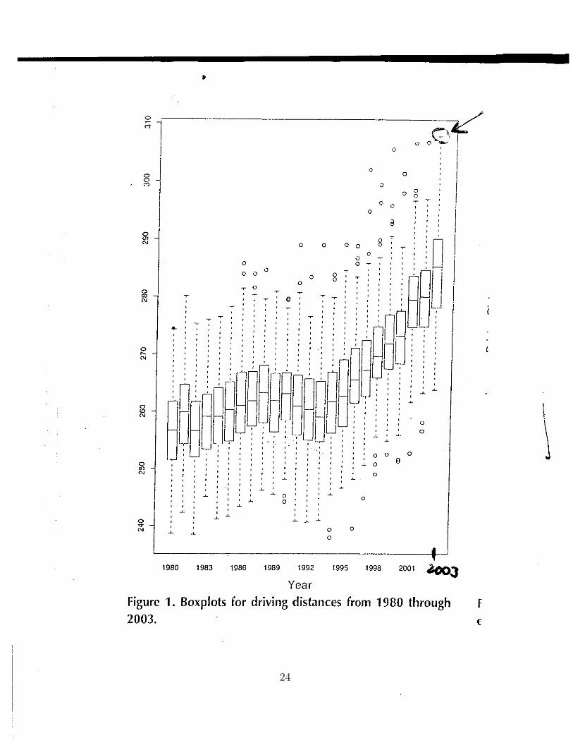
24

Lecture 05
Scatterplots:
• a graphical descriptive statistic
• for paired quantitative data (x1, y1), . . . , (xn, yn)
• always label axes and provide a title
• focus is on the relationship between x and y
• scatterplots aid in prediction
• interpolation versus extrapolation
25

Examples: data appropriate for a scatterplot?
(a) Consider 20 patients who take drug 1 and werecord their blood pressure (x’s). There are 20other patients who take drug 2 and we recordtheir blood pressure (y’s).
(b) Consider the monthly immigration rates (x’s)into British Columbia and the monthly emigra-tion rates from British Columbia (y’s).
(c) We consider 10 different colours. In a neigh-bourhood, we count the number of houses ofeach colour.
26

27

Sample correlation coefficient r:
• a numerical descriptive statistic
• for paired quantitative data (x1, y1) . . . , (xn, yn)
• r =∑
(xi−x)(yi−y)√∑(xi−x)2 ∑(yi−y)2
• r describes linearity between x and y
28

Association versus cause-effect:
• correlation does not imply causation
• the role of lurking variables in causation
• observational studies
• randomized experiments
Example for discussion: “Prayer can Lower BloodPressure”, USA Today, August 11, 1998.
People who attended a religious service once aweek and prayed or studied the Bible were 40%less likely to have high blood pressure.
29

Lecture 06
More on graphical statistics:Recall that the purpose of a graphical descrip-tive statistic is to facilitate insight with respectto the dataset. Although there are various stan-dard graphical statistics (e.g. histograms, box-plots, scatterplots), sometimes data with a non-standard structure may benefit from a special-purpose graphical display.
The only limit in developing graphical displaysis your imagination. Keep in mind however thatthe goal is to learn from the display. There-fore, simplicity and clarity are important con-siderations. On the following pages, we give anexample of a non-standard dataset and specialpurpose graphical displays that aid in address-ing various questions.
30

31

32

33

Introduction to probability:We think of an experiment as any action thatproduces data.
The sample space is the set of all possible out-comes of the experiment.
An event is a subset of the sample space.
Example 1: flipping a coin three times.
34

Example 2: total auto accidents in BC in a year
Example 3: lifespan in hours of 2 components
35

Problem: Write down the sample space wrt theexperiment where you roll a die until an evennumber occurs.
Set theory for events using Venn diagrams:
• “A union B” ≡ “A or B” ≡ A ∪B
• “A intersect B” ≡ “A and B”≡ A ∩B ≡ AB
• “A complement” ≡ A ≡ A′ ≡ Ac
36
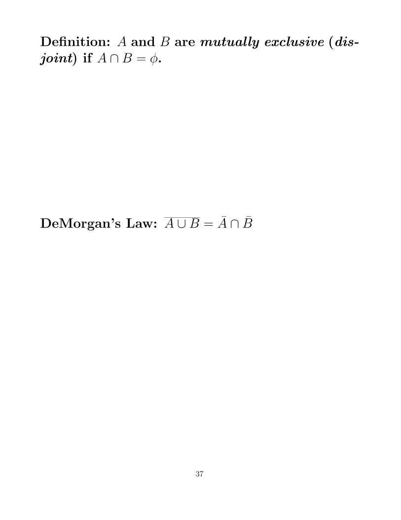
Definition: A and B are mutually exclusive (dis-joint) if A ∩B = φ.
DeMorgan’s Law: A ∪B = A ∩ B
37

Something to think about: Probability is usedin everyday language yet it is not well defined.What is meant by the statement “the probabilityof rain today is 0.7”?
Oxford English Dictionary definition of probabil-ity: extent to which an event is likely to occur,measured by the ratio of favourable cases to thewhole number of cases possible
38
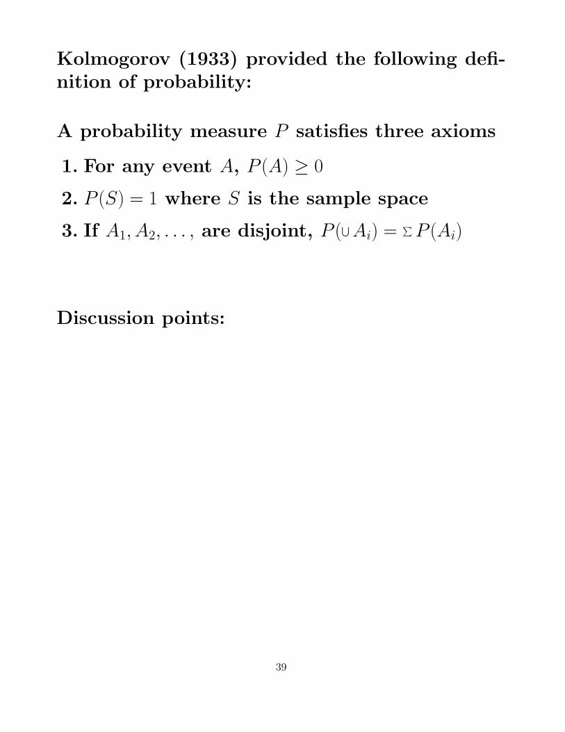
Kolmogorov (1933) provided the following defi-nition of probability:
A probability measure P satisfies three axioms
1. For any event A, P (A) ≥ 0
2. P (S) = 1 where S is the sample space
3. If A1, A2, . . . , are disjoint, P (⋃Ai) = ∑P (Ai)
Discussion points:
39

Useful derivations from the Kolmogorov defn:
Example: P (A) = 1− P (A)
Example: P (φ) = 0
Example: If A ⊆ B, P (A) ≤ P (B)
40

Example: P (A ∪B) = P (A) + P (B)− P (AB)
Example:P (A ∪B ∪ C) = P (A) + P (B) + P (C)
−P (AB)− P (AC)− P (BC)+P (ABC)
41

Lecture 07
Symmetry definition of probability:
In the case of a finite number of equally likelyoutcomes in an experiment,
P (A) =number of outcomes leading to A
number of outcomes in the experiment
Example: Roll two dice. Let A be the event thatthe sum is 10.
Discussion points:
42

Frequency definition of probability:
In hypothetical identical trials of an experiment,
P (A) = the long term relative frequency of A
Example: Roll two dice n times. Let A be theevent that the sum is 10.
Discussion points:
43

Problem: If 85% of Canadians like either base-ball or hockey, 63% like hockey and 52% likebaseball, what is the probability that a randomlychosen Canadian likes both hockey and baseball?
44

Conditional probability (an important topic):
The conditional probability of A given B is
P (A | B) =P (AB)
P (B)
provided that P (B) 6= 0.
Problem: Suppose that I roll a die and tell youthat the result is even. What is the probabilitythat the outcome is a 6?
45

Problem: The probability of surviving a trans-plant operation is 0.55. If a patient survives theoperation, the probability that the body rejectsthe transplant within a month is 0.2. What isthe probability of surviving both critical stages?
46

Confusion of the inverse: P (A | B) 6= P (B | A)
A patient has a lump in her breast. A physi-cian believes that there is a 1% chance that thelump is malignant. A mammogram is positivewhere mammograms are accurate 80% of thetime when lumps are malignant and mammo-grams are accurate 90% of the time when lumpsare benign. The test comes back positive.
What is your opinion concerning the probabilityof the malignancy of the lump?
47

Problem: In each box of my favourite cereal,there is a prize. Suppose that the cereal com-pany distributes 10 different prizes randomly inthe boxes of cereal. If I purchase five boxes ofcereal, what is the probability that I obtain fivedifferent prizes?
48

The Monty Hall problem: On the game show“Let Make a Deal”, a contestant is given thechoice of three doors. Behind one door is agrand prize (e.g. a car) and behind the othertwo doors are gag gifts. The contestant picks adoor, and Monty (who knows what is behind allof the doors), reveals a gag gift by opening oneof the two doors that the contestant has not cho-sen. Monty then gives the contestant the choiceof switching doors between the remaining twounopened doors. Should the contestant switch?
49

Lecture 08
Independence: Lets begin thinking about inde-pendence in an informal way. Two events areindependent if the occurrence or nonoccurrenceof one event does not affect the probability ofthe other event.
Formally, and this is how you are required toprove independence, events A and B are inde-pendent if and only if
P (AB) = P (A)P (B)
50

Example: Suppose that I flip a coin and roll adie. What is the probability of obtaining a tailand a six?
51

Topic for discussion: Suppose that you go toa casino and you are watching roulette. Youare thinking about placing a bet on either redor black. You have observed that the roulettewheel has resulted in a black number 6 times ina row. Do you bet red or black?
Does your opinion change if black comes up 100times in a row?
52

More on independence: There is a connectionbetween conditional probability and independence.
Proposition: Suppose P (A) 6= 0, P (B) 6= 0 and Aand B are independent. Then P (A | B) = P (A)and P (B | A) = P (B).
The converse is also true.
53

Definition: Events A1, . . . , Ak are mutually inde-pendent if and only if the probability of the in-tersection of any 2, 3, . . . , k of these events equalsthe product of their respective probabilities.
Example: Consider the case of mutual indepen-dence of the events A1, A2, A3 and A4.
54

Example of pairwise independence but not mu-tual independence: Roll two dice and define
• A1 ≡ first die is odd
• A2 ≡ second die is odd
• A3 ≡ sum of both dice is odd
55

The birthday problem: Amongst 30 people, whatis the probability that at least two of them sharea common birthday?
Generalize the problem to n people.
56

Basic combinatorial results:
Proposition: The number of permutations of ndistinct objects is n! = n(n− 1)(n− 2) · · · 1
Example: We can permute symbols A, B and Cin 3! = 6 ways.
Definition: 0! = 1.
57

Proposition: The number of permutations of robjects chosen from n distinct objects is n(r) =n!/(n− r)!
Example: We can permute two of the symbolsA, B, C, D and E in 5(2) = 5!/(5 − 2)! = 120/6 = 20ways.
58

Lecture 09
Proposition: The number of combinations of robjects chosen from n distinct objects is
nr
=n(r)
r!=
n!
r!(n− r)!
Example: We can choose two of the symbols A,
B, C, D and E in
52
= 5!2!(5−2)! = 10 ways.
59

Calculating combinations by hand: Try
304
.
Example: There are 20 people in a room. Howmany committees of four people can be chosen?
Anecdote regarding combination locks:
60

Proposition: There are
nr
ways of partitioning
n distinct objects into a first group of size r anda second group of size n− r.
Corollary:
nr
=
nn− r
61

Proposition: Let n = n1 + · · · + nk. There aren!
n1!n2!···nk! ways of partitioning n distinct objectsinto k distinct groups of sizes n1, n2, . . . , nk.
Example: How many ways can we partition thesymbols A, B, C and D into distinct groups ofsizes 1, 2 and 1?
62

Lets summarize: We have been developing count-
ing rules, specifically n!, n(r),
nr
and n!n1!n2!···nk!.
Whereas none of these rules are too difficult in-dividually, the challenge is to use the countingrules to calculate probabilities.
Using the symmetry definition, recall that theprobability of an event A is given by
P (A) =number of outcomes where A occurs
total outcomes in the experiment
Problem: In a class of 100 students, 20 are fe-male. If we randomly draw five students to forma committee, what is the probability that at leasttwo of the committee members are female?
63

Problem: In a row of four seats, two couplesrandomly sit down. What is the probability thatnobody sits beside their partner?
64

Problem: We roll a die. If we obtain a 6, wechoose a ball from box A where three balls arewhite and two are black. If we do not obtain a6, we choose a ball from box B where two ballsare white and four are black.
(a) What is the probability of obtaining a whiteball?
(b) If a white ball is chosen, what is the proba-bility that it came from box A?
65

Problem: Five cards are dealt from a deck of 52playing cards. What is the probability of
(a) three of a kind?
(b) two pair?
(c) straight flush?
66

Lecture 10
More probability calculations:
Lotto 649:
• P (jackpot)
• P (five matching numbers)
• P (four matching numbers)
• P (two matching numbers)
67

Keno calculations: similar to Lotto 649
68

Problem: There are N people who attend thetheatre and check their coats. At the end of theperformance, the coats are randomly returned.What is the probability that nobody receivestheir own coat?
69

Problem: Out of 300 woodpeckers, 30 have dam-age to the beak but not the crest, 50 have dam-age to the crest but not the beak and 10 havedamage to both the beak and crest.
(a) How many woodpeckers have no damage?
(b) For a randomly chosen woodpecker, are crestand beak damage independent?
(c) For a randomly chosen woodpecker, are crestand beak damage mutually exclusive?
70

Problem: Consider 12 balls (3 orange, 3 green,3 blue and 3 red). We randomly choose 9 ballsfrom the 12. How many different looking selec-tions can be made?
Problem: How many bridge hands are there?
Problem: If we scramble the letters R, O, T, T,N, O, and O, what is the probability that wespell TORONTO?
71

Problem: A batch of 100 stereos contains n de-fective speakers. A sample of 5 stereos is in-spected. What is the probability that y stereosare defective?
Problem: Consider a bag with 4 red marbles and6 black marbles. What is the probability of ob-taining 3 red marbles if we draw three marblesfrom the bag (i) with replacement and (ii) with-out replacement? Repeat the calculations if thebag contains 40 red and 60 black marbles.
72

Lecture 11
Coincidences are often misunderstood.
Example for discussion: Richard Baker left ashopping mall, found what he thought was hiscar and drove away. Later, he realized it wasthe wrong car and returned to the parking lot.The car belonged to another Mr Baker who hadthe same model of car, with an identical key!Police estimated the odds of this happening atone million to one.
• Were the police correct?
• How astonished should we be?
73

Example for discussion: Consider the case oftwins who were separated at birth. They latermeet as adults and are amazed that they sharesome striking characteristics (eg. they use thesame toothpaste, their eldest children have thesame names, they have the same job).
Should they be amazed?
74

Definition: A random variable (rv) is a functionof the sample space.
Example: A coin is flipped three times. Let Xbe the number of heads.
Definition: A random variable is discrete if itsoutcomes are discrete.
Definition: A random variable that takes on thevalues 0 and 1 is Bernoulli.
Example: Consider the temperature in degreesCelsius. Let Y = 1(0) if the temperature is freez-ing (not freezing).
75
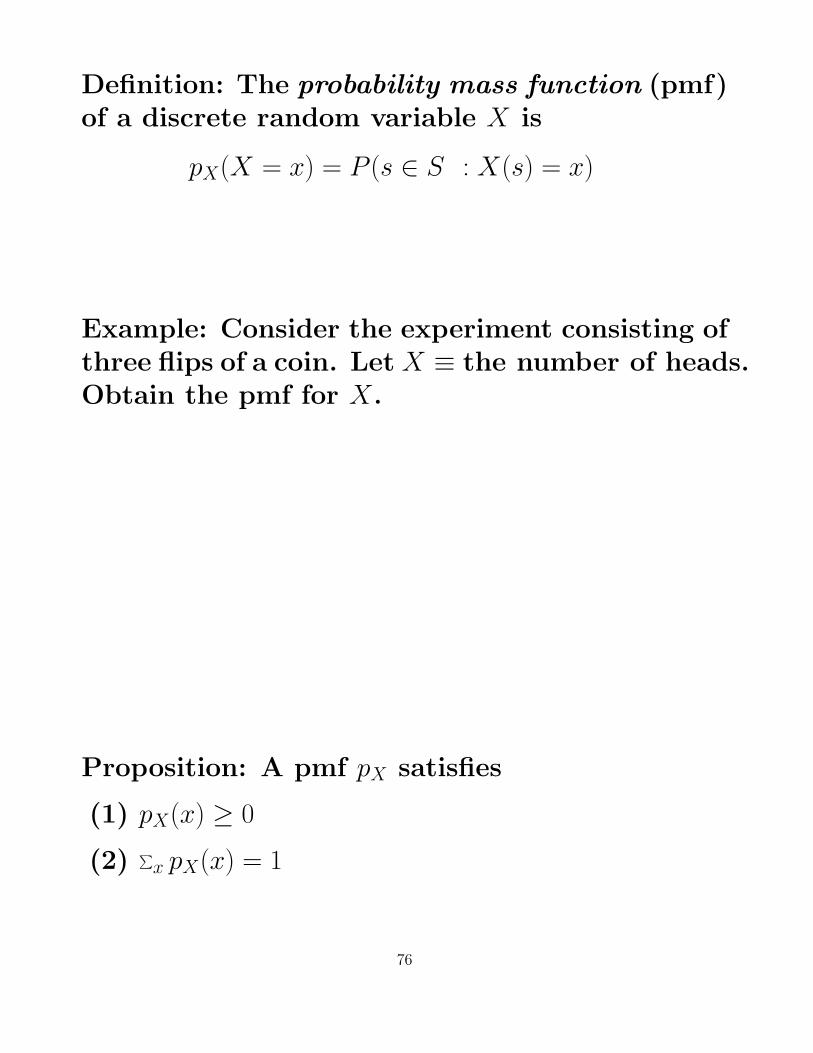
Definition: The probability mass function (pmf)of a discrete random variable X is
pX(X = x) = P (s ∈ S : X(s) = x)
Example: Consider the experiment consisting ofthree flips of a coin. Let X ≡ the number of heads.Obtain the pmf for X.
Proposition: A pmf pX satisfies
(1) pX(x) ≥ 0
(2) ∑x pX(x) = 1
76

Example: Let X be the sum of two dice. Obtainthe pmf of X.
Example: Consider a batter with a 300 average.Let X be the number of at bats until the battergets a hit. Obtain the pmf of X.
77

Problem: A library subscribes to two weeklymagazines, each of which is suppose to arriveon Wednesdays. In actuality, the two maga-zines arrive independently with probabilities ofarrival, P (Wed) = 0.3, P (Thu) = 0.4, P (Fri) = 0.2 andP (Sat) = 0.1. Let Y be the number of days beyondWednesday that it takes for both magazines toarrive. Obtain the pmf of Y .
78

Problem: At the end of an exam, four textbooksare left behind. At the beginning of the nextlecture, the four texts are randomly returnedto the four students. Let X be the number ofstudents who receive their own book. Obtainthe pmf of X.
79

Lecture 12
Definition: The cumulative distribution func-tion (cdf) of a random variable X with probabil-ity measure PX is given by
FX(x) = PX(X ≤ x)
Example: Consider three flips of a coin and letX be the number of heads. Obtain the cdf of X.
Properties of a cdf F :
(1) F is normed (i.e. F (−∞) = 0, F (∞) = 1)
(2) F is monotone increasing
(3) F is right continuous
80

Given a cdf corresponding to a discrete distribu-tion, be able to determine the pmf.
Example:
81

Definition: The expectation of a discrete rv Xwith pmf p(x) is given by
µ ≡ E(X) ≡ ∑xx p(x)
The expectation can be thought of the long runaverage of the random variable over hypotheticalrepetitions of the experiment.
Example: Consider the experiment consisting ofthree flips of a coin. Let X ≡ the number of heads.Obtain E(X).
82

Example: Consider the experiment of tossing adie and let X be the outcome. Obtain E(X).
Earlier it was stated that we view the expecta-tion of a random X as the long run average ofX. Lets explore this statement by considering Nhypothetical repetitions of the experiment.
83

Proposition: The expectation of a function g(X)corresponding to the discrete random variable Xwith pmf p(x) is given by
E(g(X)) =∑xg(x) p(x)
Example: Consider the experiment of tossing adie and let X be the outcome. Obtain E(X2).
Proposition: E(aX + b) = aE(X) + b
84

Problem: A store orders copies of a weekly mag-azine for its magazine rack. Let X be the weeklydemand for the magazine with pmf
x 1 2 3 4 5 6p(x) 1
15215
315
415
315
215
Suppose that the store owner pays $1 for eachcopy of the magazine and the customer price is$2. If leftover magazines at the end of the weekhave no salvage value, is it better for the ownerto order three magazines or four magazines?
85

Is expectation always a reasonable criterion?
Problem for discussion: Suppose that you aregiven the chance to play a game a single timewhere the entrance fee is $1 million dollars. Withprobability 0.99, you lose and receive nothing.With probability 0.01, you win and receive $1billion dollars. Should you play the game?
86

Lecture 13
We explore expectation in more detail.
Proposition: For a discrete rv X with pmf p(x)
E(g1(x) + · · · + gk(x)) = E(g1(x)) + · · · + E(gk(x))
Definition: The variance of a discrete rv X withpmf p(x) is
σ2 ≡ V(X) ≡ E[(X − E(X))2]
• we call σ the standard deviation
• σ and σ2 are measures of spread
• contrast sample quantities (x, s) with poplnquantities (µ, σ)
87

Example: Consider the experiment consisting ofthree flips of a coin. Let X ≡ the number of heads.Obtain V(X).
Proposition: V(X) = E(X2)− (E(X))2
88

Proposition: V(aX + b) = a2V(X)
Example: Let X be the average january temper-ature in degrees Celsius where E(X) = 5C andV(X) = 3(C)2. Find the expected value and thevariance of Y where Y is the average januarytemperature in degrees Fahrenheit.
89

Problem: Calculate σ and E(3X + 4X2) corre-sponding to the rv X with pmf p(x) where
x 4 8 10p(x) 0.2 0.7 0.1
90

Example: In a game of chance, I bet x dollars.With probability p, I win y dollars. What shouldx be for this to be a fair game?
91

Definition: A discrete rv X has a Binomial dis-tribution denoted Bin(n, θ) if it has pmf
p(x) =
nx
θx(1− θ)n−x x = 0, 1, . . . , n
0 otherwise
92

Motivation for the Binomial - the most impor-tant discrete distribution:
Consider performing an experiment n times wherethe probability of success in every trial is θ andthe n experiments are independent. We are in-terested in the probability of x successes.
The probability of getting x successes S and n−xfailures F in the specific order
SS · · ·S FF · · ·F
is
θθ · · · θ (1− θ)(1− θ) · · · (1− θ)= θx(1− θ)n−x.
Therefore
P (x successes) =
nx
θx(1− θ)n−x
for x = 0, 1, . . . , n.
93
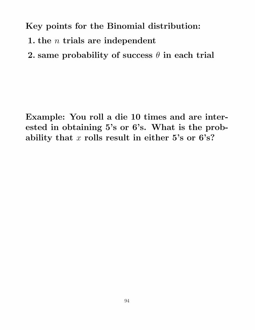
Key points for the Binomial distribution:
1. the n trials are independent
2. same probability of success θ in each trial
Example: You roll a die 10 times and are inter-ested in obtaining 5’s or 6’s. What is the prob-ability that x rolls result in either 5’s or 6’s?
94

For X ∼ Bin(n, θ)
• E(X) = nθ
• V(X) = nθ(1− θ)
Proof (first result):
E(X) = Σnx=0 x
nx
θx(1− θ)n−x
= Σnx=1 x
n!x!(n−x)! θ
x(1− θ)n−x
= nθ Σnx=1
(n−1)!(x−1)!(n−x)! θ
x−1(1− θ)n−x
= nθ Σn−1y=0
(n−1)!y!(n−1−y)! θ
y(1− θ)n−1−y
= nθ Σn−1y=0
n− 1y
θy(1− θ)n−1−y
= nθ
95

Lecture 14
Problem: A friend recently planned a camp-ing trip. He had two flashlights, one that re-quired a single 6-V battery and another thatused two size-D batteries. He had previouslypacked two 6-V and four size-D batteries in hiscamper. Suppose that the probability than anyparticular battery works is p and that batterieswork or fail independently of one another. Ourfriend wants to take just one flashlight. For whatvalues of p should he take the 6-V flashlight?
96

Problem: A k-out-of-n system is one that func-tions if and only if at least k of the n individualcomponents in the system function. If individ-ual components function independently of oneanother, each with probability 0.9, what is theprobability that a 3-out-of-5 system functions?
How many components do you expect to workin a 3-out-of-5 system?
97

Problem: Suppose that only 20% of all driverscome to a complete stop at an intersection hav-ing flashing red lights in all directions when noother cars are visible. What is the probabilitythat, of 20 randomly chosen drivers coming toan intersection under these conditions,
(a) at most six will come to a complete stop?
(b) exactly six will come to a complete stop?
(c) at least six will come to a complete stop?
(d) How many of the next 20 drivers do youexpect to come to a complete stop?
98

Problem: A baseball player with a 300 averagehas 600 at-bats (attempts) in a season.
(a) Propose a pmf for the number of hits X.
(b) Is the probability distribution reasonable?
(c) What is the expected number of hits?
99

Definition: A rv X has a Poisson(λ) distribution,λ > 0, if it has pmf
p(x) =λxe−λ
x!x = 0, 1, 2, . . .
The Poisson distribution is especially good atmodelling rare events (more later).
100

For X ∼ Poisson(λ)
• E(X) = λ
• V(X) = λ
Proof (first result):
E(X) = Σ∞x=0 x λxe−λ/x!
= e−λ Σ∞x=1 x λx/x!
= e−λλ Σ∞x=1 λx−1/(x− 1)!
= e−λλ Σ∞y=0 λy/y!
= e−λλ eλ
= λ
101

Time for some fun (not related to Poisson)!
15 + 6
3 + 56
89 + 2
53 - 12
75 + 26
-7 - 9
123 + 5
Quick: Think about a and a .
102

Lecture 15
Recall that the Binomial pmf may be difficult tocalculate. It turns out the Binomial can some-times be approximated by the Poisson.
Proposition: Without being rigorous, Bin(n, θ) ≈Poisson(nθ) if n is much larger than nθ.
103

Example: A rare type of blood occurs in a pop-ulation with frequency 0.001. If n people aretested, what is the probability that at least twopeople have this rare blood type? Calculate theprobability using the Binomial distribution andthe Poisson approximation to the Binomial.
104
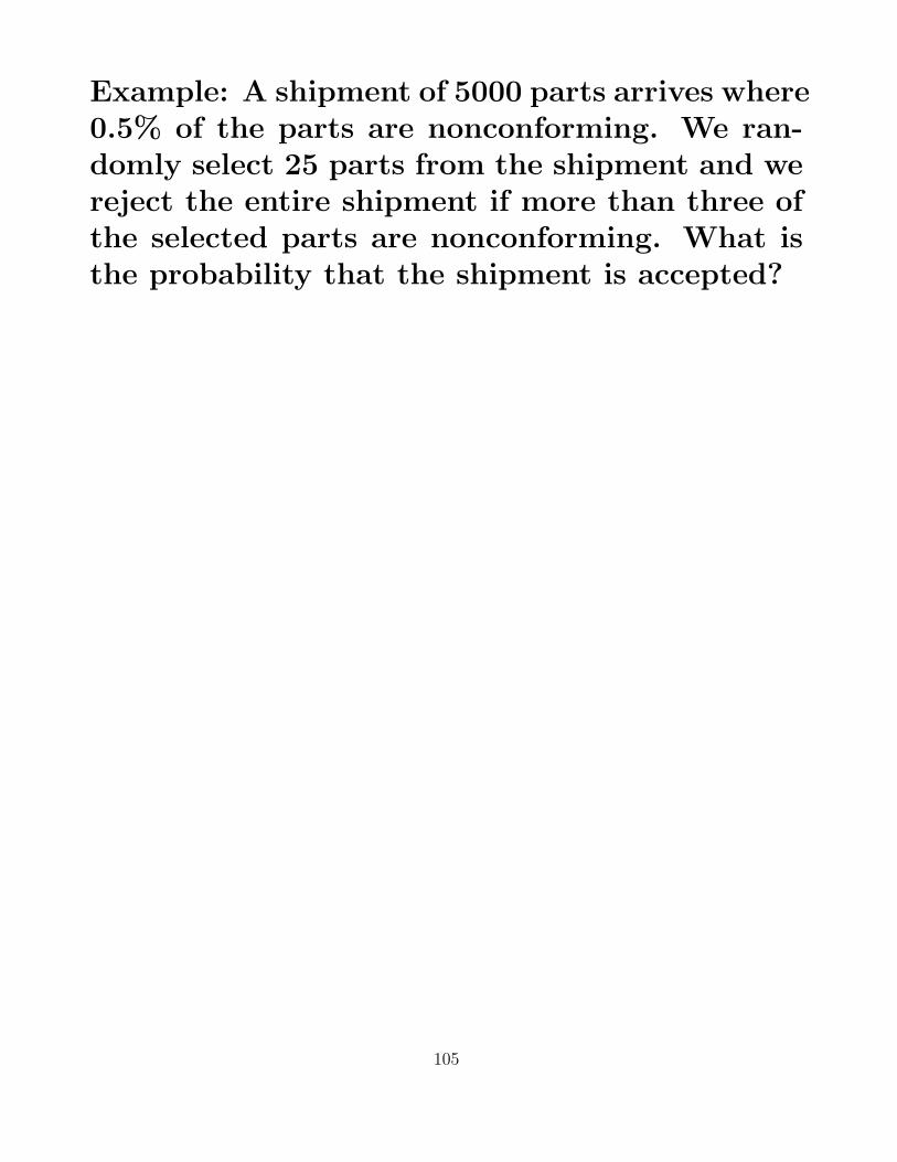
Example: A shipment of 5000 parts arrives where0.5% of the parts are nonconforming. We ran-domly select 25 parts from the shipment and wereject the entire shipment if more than three ofthe selected parts are nonconforming. What isthe probability that the shipment is accepted?
105

Recall that the Binomial distribution can be mo-tivated by considering n independent trials wherethe probability of success on each trial is con-stant. Similarly, the Poisson distribution can bemotivated by three assumptions which comprisethe Poisson process. The assumptions of thePoisson process are these:
1. events are indpt in non-overlapping intervals
2. events are stationary
3. during small time intervals, the probability ofa single event is proportional to the length ofthe time interval and the probability of morethan one event is negligible
106

Proposition: Let p(x, t) be the probability of xsuccesses in an interval of length t. Under theassumptions of the Poisson process
p(x, t) =(λt)xe−λt
x!x = 0, 1, . . .
107

Example: A switchboard receives calls at a rateof three per minute during a busy period. Let Xt
denote the number of calls in t minutes during abusy period. Assess whether the assumptions ofa Poisson process are reasonable. Then, assum-ing the assumptions are reasonable, calculate theprobability of receiving more than three calls ina two-minute interval during a busy period.
108

Lecture 16
Review problem: A limousine can accommodateup to four passengers. The company accepts upto six reservations and passengers must have areservation to travel. From records, 20% of pas-sengers with reservations do not show.
(a) If six reservations are made, what is theprobability that at least one passenger can-not be accommodated?
(b) If six reservations are made what is the ex-pected number of available places when thelimousine departs?
(c) Suppose that the pmf of the number of reser-vations R is
r 3 4 5 6p(r) 0.1 0.2 0.3 0.4
Find the pmf of the number of passengers Xwho show up.
109

Definition: A rv is continuous if it takes on realvalues in an interval.
Example: Let X be the temperature in degreesCelsius at SFU.
Definition: Let X be a continuous rv. Then theprobability density function (pdf) f (x) ≥ 0 of Xis such that
P (a ≤ X ≤ b) =∫ ba f (x) dx ∀a < b
Proposition: The function f (x) is a pdf if
1. f (x) ≥ 0 and
2.∫ ∞−∞ f (x) dx = 1
110

Problem: Verify that f (x) is a pdf where
f (x) =
0 x ≤ 0x 0 < x ≤ 1
1/2 1 < x ≤ 20 2 < x
Calculate Prob(1 ≤ X ≤ 1.5).
111

Definition: A rv X has a Uniform(a, b) distribu-tion if it has pdf
f (x) =1
b− aa < x < b
Special case: Uniform(0,1)
112

Definition: The cumulative distribution func-tion (cdf) of a continuous rv X is given by
F (x) = P(X ≤ x) =∫ x−∞ f (y) dy a < x < b
Definition: The 100p-th percentile of the contin-uous distribution with cdf F (x) is the value η(p)such that
p = F (η(p))
Definition: The median µ of the continuous dis-tribution with cdf F (x) is the 50-th percentile(i.e. 0.5 = F (µ)).
113

Example: Find the median of the Uniform(a, b)distribution.
114

Definition: The expected value of a continuousrv X with pdf f (x) is
µ = E(X) =∫ ∞−∞ xf (x) dx a < x < b
Proposition: If X is a continuous rv with pdff (x)
E(g(X)) =∫ ∞−∞ g(x)f (x) dx
Definition: The variance of a continuous rv Xwith pdf f (x) is
V(X) = E((X − E(X))2) =∫ ∞−∞ (x− E(X))2f (x) dx
115

Proposition: If X is a continuous rv, then as inthe discrete case,
• V(X) = E(X2)− (E(X))2
• E(aX + b) = aE(X) + b
• V(aX + b) = a2V(X)
116

Lecture 17
Problem: Consider the pdf of the rv Y
f (y) =
y/25 0 ≤ y < 52/5− y/25 5 ≤ y < 10
(a) obtain the cdf of Y
(b) calculate the 100p-th percentile of Y
(c) calculate E(Y )
117

Problem: Let X be the time in hours that areserved book is checked out by a randomly se-lected student. Suppose that X has the densityfunction
f (x) =
x/2 0 ≤ x ≤ 20 otherwise
(a) calculate P(X ≤ 1)
(b) calculate P(0.5 ≤ X ≤ 1.5)
(c) calculate P(0.5 < X)
118

Problem: A professor never finishes lectures be-fore the end of the hour and always finishes withintwo minutes after the hour. Let X be the timethat elapses between the end of the hour and theend of the lecture and suppose the pdf of X is
f (x) =
kx2 0 ≤ x ≤ 20 otherwise
(a) evaluate k
(b) what is the probability that the lecture endswithin one minute of the end of the hour?
(c) what is the probability that the lecture con-tinues beyond the hour for between 60 and 90seconds?
(d) what is the probability that the lecture con-tinues for at least 90 seconds beyond the endof the hour?
119

Problem: The cdf of checkout duration in min-utes X is
F (x) =
0 x < 0x2/4 0 ≤ x ≤ 2
(a) calculate P(0.5 ≤ X ≤ 1)
(b) calculate the median of X
(c) calculate the pdf of X
(d) calculate E(X)
120

Without doubt, the most important distributionin all of Statistics is the normal (Gaussian) dis-tribution.
Definition: A rv X has a Normal(µ, σ2) distribu-tion if it has pdf
f (x) =1√
2πσ2exp
−1
2
x− µσ
2
where x ∈ R, µ ∈ R and σ > 0.
Some talking points:
• the normal is a family of distributions
• the density is symmetric about µ
• the density never touches zero
• the density is not tractable
• the parameters are interpretable: E(X) = µand V(X) = σ2
• data are often approximately normal
• the standard normal distribution is Normal(0, 1)and is typically represented by the rv Z
121

To gain an understanding of the parameters µand σ, sketch plots of the following distributions:
• Normal(5, 1)
• Normal(7, 1)
• Normal(5, 10)
• Normal(5, 1/10)
122

You must become familiar with the standardnormal table (Table B.2 in the text). Calculatethe following:
(a) P(Z ≤ 3.02)
(b) P(Z > 3.03)
(c) P(Z < 3.025) via interpolation
(d) P(2.3 ≤ Z ≤ 2.6)
(e) P(Z > −1)
(f) z such that 30.5% of Z-values exceed z
123

Lecture 18
Proposition: If X ∼ Normal(µ, σ2), then
Z =X − µσ∼ Normal(0, 1)
A consequence is that any normal probabilitycan be converted to a probability involving thestandard normal. This means that we only needa single normal table instead of tables for allpossible values of µ and σ.
Problem: The number of hours that people watchtelevision is normally distributed with mean 6.0hours and standard deviation 2.5 hours (first askyourself if this is reasonable). What is the prob-ability that a randomly selected person watchesmore than 8 hours of television per day?
124

Problem: The substrate concentration (mg/cm3)of influent to a reactor is normally distributedwith µ = 0.30 and σ = 0.06.
(a) What is the probability that the concentra-tion exceeds 0.25?
(b) What is the probability that the concentra-tion is at most 0.10?
(c) How would you characterize the largest 5%of all concentration values?
125

An amusing but real problem: My wife was ex-pecting on June 1. My friends wanted me to goon a golf trip May 14, 15 and 16. What to do?
126

Proposition: Let η(p) denote the 100p-th per-centile of the standard normal distribution. Thenthe 100p-th percentile of the Normal(µ, σ2) distri-bution is µ + ση(p).
Example: Find the 25.78-th percentile of theNormal(5, 100).
127

Proposition: Consider X ∼ Bin(n, p) where np ≥ 5and n(1 − p) ≥ 5. Then we have the followingapproximation
X ∼ Normal(np, np(1− p))
Example: Obtain P(X ≥ 8) where X ∼ Bin(10, 1/2)
(a) exactly
(b) using the normal approximation
(c) using the normal approximation with a con-tinuity correction.
128

Reminders:
(1) Probabilities associated with the Bin(n, p) aresometimes difficult to evaluate. The followingapproximations are available:
(a) Poisson(np) if n is large and p is small
(b) Normal(np, np(1− p)) if np ≥ 5 and n(1− p) ≥ 5
(2) Use a continuity correction whenever youneed to approximate a discrete distribution witha continuous distribution.
129

Lecture 19
Problem: Verbal SAT scores are normally dis-tributed with a mean score of 430 and variance100. What is the middle range of scores encom-passing 50% of the population?
130

Problem: The automatic opening device of amilitary parachute is designed to open when theparachute is 200 metres above ground. Supposethat the opening altitude has a normal distri-bution with mean 200m and standard deviation30m. Equipment damage occurs if the parachuteopens at an altitude of less than 100m aboveground. What is the probability that there isequipment damage to at least one of five inde-pendently dropped parachutes?
131

Problem: The temperature reading from a ther-mocouple in a constant-temperature medium isnormally distributed with mean µ (the actualtemperature of the medium) and standard devi-ation σ. What is the value of σ such that 95% ofall readings are within 0.1 degree of µ?
132

Problem: A patient is hypokalemic if their levelof potassium is 3.5 or less. An individual’s levelis not constant, but varies daily. Suppose thatthe variation is normal. Judy has a mean level of3.8 with variance 0.04. If she is measured daily,what proportion of days would she be declaredhypokalemic?
133

Problem: A college has a target enrollment of1200 students. Since not all admitted studentsactually enroll, the college admits 1500 students.Past experience shows that 70% of students whoare offered admission enroll.
(a) Give a statistical model for the number ofstudents who enroll.
(b) Obtain the corresponding mean and std dev.
(c) Obtain the prob that at least 1200 enroll.
134

Problem: The volume placed in a bottle by abottling machine follows a Normal(µ, σ2) distribu-tion. Over a long period of time, it is observedthat 5% of the bottles contain less than 31.5ozand 15% contain more than 32.3oz.
(a) Find µ and σ.
(b) Calculate the probability that out of 10 bot-tles purchased, exactly three bottles containmore than 32.2 oz.
135

Lecture 20
Problem: The weight distribution of parcels isnormal with mean value 12lb and std dev 3.5lb.The parcel service wants to establish a weight cbeyond which there is a surcharge. What is thevalue of c such that 99% of parcels are at least1lb under the surcharge weight?
136

Problem: The breakdown voltage of a randomlychosen diode is normally distributed with mean40V and standard deviation 1.5V.
(a) What is the probability that the voltage ofa single diode is between 39V and 42V?
(b) What value is such that only 15% of diodeshave voltages exceeding that value?
(c) If four diodes are randomly selected, what isthe probability that at least one has voltageexceeding 42V?
137

Definition: A rv X has a Gamma(α, β) distribu-tion, α > 0, β > 0, if it has pdf
f (x) =xα−1e−x/β
βαΓ(α)x > 0
where Γ(α) =∫ ∞
0 xα−1e−x dx
Discussion points:
• pdf generally intractable
• contrast the range (x > 0) with the normal
• asymmetric
• Γ(α) is a constant
• Γ(α) = (α− 1)Γ(α− 1), Γ(1) = 1, Γ(1/2) =√π
138

Proposition: If X ∼ Gamma(α, β), then
• E(X) = αβ
• V(X) = αβ2
139

The Exponential(λ) distribution is a special case ofthe Gamma(α, β) where α = 1 and β = 1/λ.
Definition: A rv X has an Exponential(λ) distribu-tion, λ > 0, if it has pdf
f (x) = λe−λx x > 0
Discussion points:
• E(X) = αβ = 1(1/λ) = 1/λ
• V(X) = αβ2 = 1(1/λ)2 = 1/λ2
• the density is decreasing for x > 0
• the density is tractable; in particular the cdfF (x) = 1− e−λx for x > 0
140

The Exponential distribution possesses a curiousproperty known as the memoryless property. Toappreciate the property, consider a rv X whichis the lifespan of a lightbulb in hours where weassume that X ∼ Exponential(λ). Then the prob-ability that a used lightbulb (that has alreadylasted a hours) will last an additional b hours isgiven by
P(X > a + b | X > a) =
141

Lecture 21
It turns out that there is a connection betweenthe Poisson and Exponential distributions. Re-call the Poisson process where NT is the numberof events that occur in the interval [0, T ] whereNT ∼ Poisson(λT ). Let
Y ≡ waiting time until the first event
Then the cdf of Y is given by
P(Y ≤ y) = 1− P(Y > y)= 1− P(zero events in [0,y])= 1− P(Ny = 0) where Ny ∼ Poisson(λy)= 1− (λy)0e−λy/0!= 1− e−λy
which implies Y ∼ Exponential(λ)
142

Problem: Let X be the distance in metres thata rat moves from its birth site to its first territo-rial vacancy. Suppose that X has an exponentialdistribution with λ = 0.01386.
(a) What is the probability that the distance Xis at most 100 metres?
(b) What is the probability that the distance Xexceeds the mean distance by more than twostandard deviations?
(c) What is the median distance?
143

Until now, we have studied probabilities corre-sponding to a single rv X. We now considerjoint probability distributions associated with avector rv (X1, . . . , Xk).
Example: a trivariate discrete distribution de-scribed by the pmf p(x, y, z)
X=1 X=2 X=3Y=1 0.10 0.20 0.00Y=2 0.00 0.05 0.05
Z = 5
X=1 X=2 X=3Y=1 0.00 0.30 0.10Y=2 0.05 0.05 0.10
Z = 6
The marginal pmf p(x) = Σy,zp(x, y, z)
144

In the continuous setting, we describe distribu-tions via a joint pdf f (x1, . . . , xk) which satisfies
1. f (x1, . . . , xk) ≥ 0 ∀ x1, . . . , xk
2.∫ ∞−∞ · · ·
∫ ∞−∞ f (x1, . . . , xk) dx1 · · · dxk = 1
To obtain probabilities in the continuous setting,
P((X1, . . . , Xk) ∈ A) =∫· · ·
∫A f (x1, . . . , xk) dx1 · · · dxk
145

Example: A bivariate distribution on (X, Y ) isgiven by f (x, y) = 2(2x + 3y)/5 where 0 < x, y < 1
(a) Calculate P(X > 1/2, Y < 1/2).
(b) Obtain the marginal pdf of X and verify thatit is a pdf.
146

Recall that we previously discussed the indepen-dence of events. The concept of independencecan be extended to rv’s.
Definition: Random variables are independent iftheir joint pmfs (pdfs) factor into their marginalpmfs (pdfs).
Example: Consider the bivariate pdf
f (x, y) =1
2πσ1σ2exp
−1
2
(x2/σ2
1 + y2/σ22
)
=1√
2πσ21
exp
−1
2
x− 0
σ1
2
1√2πσ2
2
exp
−1
2
y − 0
σ2
2
147

Example: Consider the bivariate pmf given by
X=1 X=2Y=1 0.4 0.2Y=2 0.1 0.3
(a) Obtain the marginal pmf for X.
(b) Obtain the marginal pmf for Y .
(c) Are X and Y independent?
148

Problem: Two components of a computer havethe joint pdf for their lifetimes X and Y in years
f (x, y) = xe−x(1+y) x, y ≥ 0
(a) What is the probability that the lifetime Xof the first component exceeds 3 years?
(b) What are the marginal pdfs of X and Y ?
(c) What is the probability that the lifetime ofat least one component exceeds 3 years?
149

Lecture 22
We now turn our attention to the expectationof functions of random variables.
Proposition: In the continuous case, using stan-dard notation,
E[g(X1, . . . , Xk)] =∫· · ·
∫g(x1, . . . xk)f (x1, . . . xk) dx1 · · · dxk
In the discrete case, we replace the pdf f withthe corresponding pmf p and we replace the mul-tiple integral with a multiple sum.
150

Example: An instructor gives a quiz with twoparts. For a randomly selected student, let Xand Y be the scores obtained on the two partsrespectively. The table gives the joint pmf p(x, y)of X and Y :
p(x,y) y=0 y=5 y=10 y=15x=0 0.02 0.06 0.02 0.10x=5 0.04 0.15 0.20 0.10x=10 0.01 0.15 0.14 0.01
(a) What is the expected total score E(X + Y )?
(b) What is the expected maximum score fromthe two parts?
(c) Are X and Y independent?
(d) Obtain P(Y = 10 | X ≥ 5).
151

Example: We return to the discrete distributiondescribed by the pmf p(x, y, z)
X=1 X=2 X=3Y=1 0.10 0.20 0.00Y=2 0.00 0.05 0.05
Z = 5
X=1 X=2 X=3Y=1 0.00 0.30 0.10Y=2 0.05 0.05 0.10
Z = 6
Obtain E(g) where g(x, y, z) = xz.
152

Problem: Annie and Alvie agree to meet forlunch between noon and 1pm. Denote Annie’sarrival time by X and Alvie’s by Y , and supposeX and Y are independent with pdfs fX(x) = 3x2
where 0 < x < 1 and fY (y) = 2y where 0 < y < 1.
What is the expected time that the one who ar-rives first waits for the other person to arrive?
153
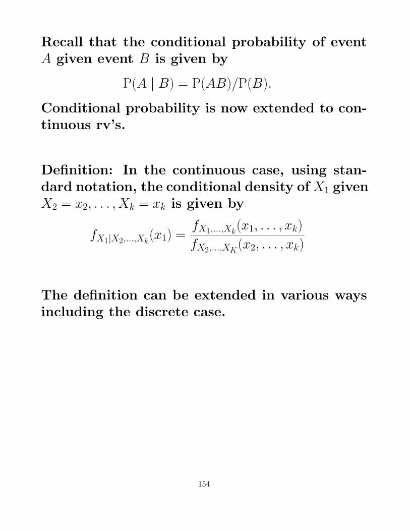
Recall that the conditional probability of eventA given event B is given by
P(A | B) = P(AB)/P(B).
Conditional probability is now extended to con-tinuous rv’s.
Definition: In the continuous case, using stan-dard notation, the conditional density of X1 givenX2 = x2, . . . , Xk = xk is given by
fX1|X2,...,Xk(x1) =fX1,...,Xk(x1, . . . , xk)
fX2,...,XK(x2, . . . , xk)
The definition can be extended in various waysincluding the discrete case.
154

Example: Recall the bivariate distribution on(X, Y ) given by the pdf fX,Y (x, y) = 2(2x + 3y)/5where 0 < x, y < 1. Earlier we established themarginal density for X given by fX(x) = 4x/5+3/5where 0 < x < 1. Suppose we observe X = 0.2.What is the conditional pdf of Y ?
155
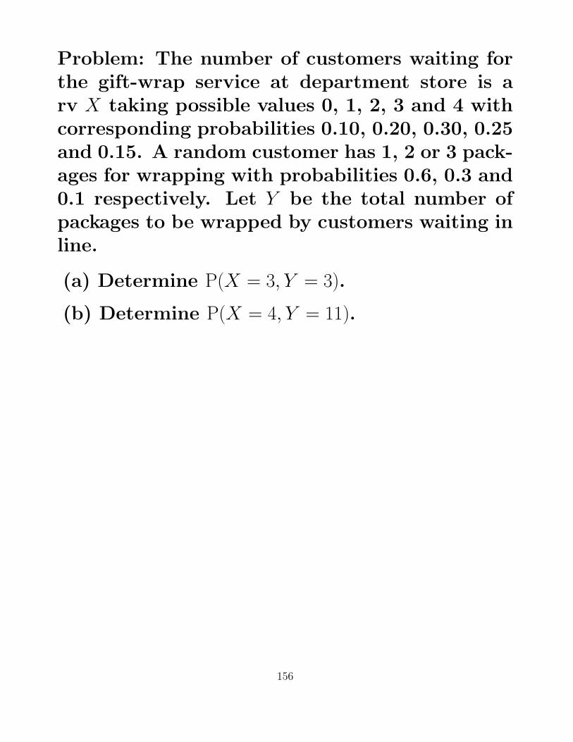
Problem: The number of customers waiting forthe gift-wrap service at department store is arv X taking possible values 0, 1, 2, 3 and 4 withcorresponding probabilities 0.10, 0.20, 0.30, 0.25and 0.15. A random customer has 1, 2 or 3 pack-ages for wrapping with probabilities 0.6, 0.3 and0.1 respectively. Let Y be the total number ofpackages to be wrapped by customers waiting inline.
(a) Determine P(X = 3, Y = 3).
(b) Determine P(X = 4, Y = 11).
156

Lecture 23
Definition: The covariance between the rvs Xand Y is given by
Cov(X, Y ) = E( (X − E(X))(Y − E(Y )) )
= E(XY )− E(X)E(Y )
Interpretation:
• positive covariance
– large x’s occur with large y’s
– small x’s occur with small y’s
• negative covariance
– large x’s occur with small y’s
– small x’s occur with large y’s
157

Correlation is the scaled and preferred versionof covariance.
Definition: The correlation between the rvs Xand Y is given by
ρ = Corr(X, Y ) =Cov(X, Y )√V(X)
√V(Y )
Discussion points:
• −1 ≤ Corr(X, Y ) ≤ 1
• correlation is location/scale invariant
• ρ is the population analogue of r
• ρ typically relevant to continuous rvs
• if a > 0, then Corr(X, aX + b) = 1
• if a < 0, then Corr(X, aX + b) = −1
158

Example: Obtain the correlation between X andY where the joint pmf of X and Y is given in thefollowing table.
X=1 X=2 X=3Y=1 0.1 0.2 0.3Y=2 0.0 0.2 0.2
159

Proposition: If X and Y are independent, then
Cov(X, Y ) = 0
In addition, Corr(X, Y ) = 0 provided V(X) andV(Y ) are nonzero. The converse is not true.
Also, recall that correlation does not imply cau-sation.
160

Proposition: V(X + Y ) = V(X) + V(Y ) + 2Cov(X, Y )
Proposition: More generally,
V(aX + bY + c) = a2V(X) + b2V(Y ) + 2abCov(X, Y )
Proposition: Even more generally,
V n∑i=1aiXi + c
= ∑ni=1 a
2iV(Xi) + 2 ∑
i<j aiajCov(Xi, Xj)
E n∑i=1aiXi + c
= c + ∑ni=1 aiE(Xi)
161

Lets put some of this stuff together to provide auseful result.
Corollary: Suppose that the rv’s X1, . . . , Xn are asample. In other words, the X’s are independentand arise from a common distribution with meanµ and variance σ2. Then the sample mean has thefollowing properties:
• E(X) = µ
• V(X) = σ2/n
162

Suprisingly, we have reached this point in ourStatistics course and we have not yet defined theword statistic.
Definition: A statistic is a function of the data.
Some examples:
• X =∑ni=1Xi/n is a statistic
• S2 =∑ni=1(Xi − X)2/(n− 1) is a statistic
Since data are variable, statistics are also vari-able. Sometimes we are interested in the distri-butions of statistics.
163
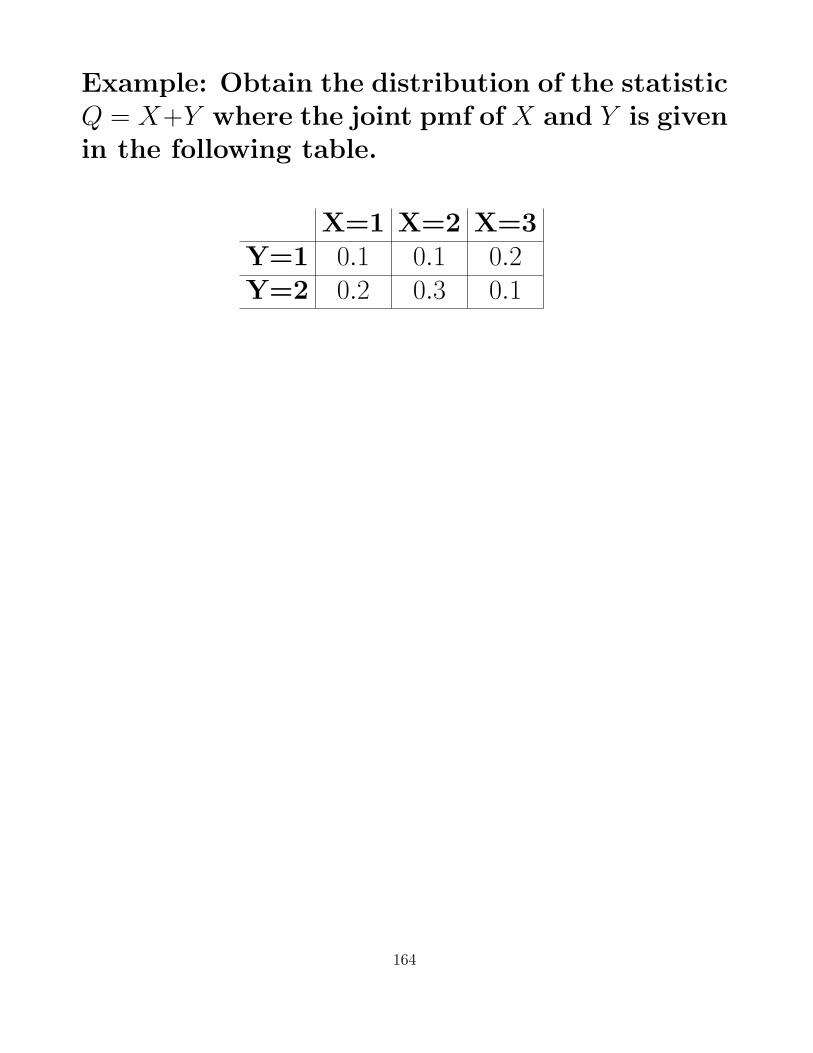
Example: Obtain the distribution of the statisticQ = X+Y where the joint pmf of X and Y is givenin the following table.
X=1 X=2 X=3Y=1 0.1 0.1 0.2Y=2 0.2 0.3 0.1
164

The previous example was simple. To generalize,we need to go a little crazy with notation.
Suppose that X1, . . . , Xn are discrete with jointpmf p(x1, . . . , xn). Then the pmf for the generalstatistic Q(X1, . . . , Xn) is
pQ(q) =∑Ap(x1, . . . , xn)
where the sum is a multiple sum and A is the setof x1, . . . , xn such that Q(x1, . . . , xn) = q.
Suppose that X1, . . . , Xn are continuous with jointpdf f (x1, . . . , xn). Then the cdf for the generalstatistic Q(X1, . . . , Xn) is
FQ(q) = P(Q ≤ q) =∫A f (x1, . . . , xn) dx1 . . . dxn
where the integral is a multiple integral and A isthe set of x1, . . . , xn such that Q(x1, . . . , xn) ≤ q.
165
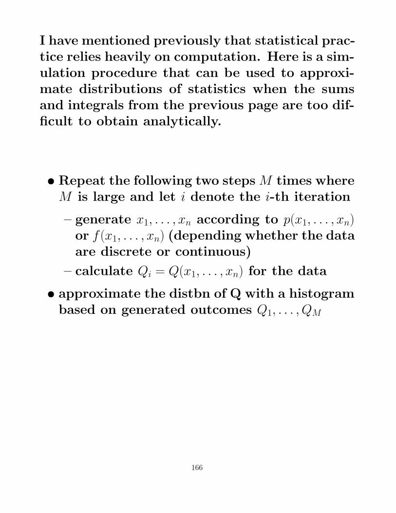
I have mentioned previously that statistical prac-tice relies heavily on computation. Here is a sim-ulation procedure that can be used to approxi-mate distributions of statistics when the sumsand integrals from the previous page are too dif-ficult to obtain analytically.
• Repeat the following two steps M times whereM is large and let i denote the i-th iteration
– generate x1, . . . , xn according to p(x1, . . . , xn)or f (x1, . . . , xn) (depending whether the dataare discrete or continuous)
– calculate Qi = Q(x1, . . . , xn) for the data
• approximate the distbn of Q with a histogrambased on generated outcomes Q1, . . . , QM
166

Lecture 24
Proposition: Linear combinations of normal rv’sare normal.
Corollary: Suppose that X1, . . . , Xn is a samplefrom the Normal(µ, σ2) distribution. Then
X ∼ Normal(µ, σ2/n)
167

Example: Determine the distribution of the rvY = 2X1 − X2 + 3X3 + 3 where X1, X2 and X3 areindependent, X1 ∼ Normal(4, 3), X2 ∼ Normal(5, 7)and X3 ∼ Normal(6, 4).
Example: Determine the distribution of the rvY = X1−X2 where Cov(X1, X2) = 6, X1 ∼ Normal(5, 10)and X2 ∼ Normal(3, 8).
168

You are not responsible for complete understand-ing of the following example. However, it givessome insight as to why linear combinations ofnormals are normal.
Example: When X and Y are independent stan-dard normal, then Z = X + Y ∼ Normal(0, 2).
P(Z ≤ z) =∫ ∞y=−∞
∫ z−yx=−∞
1√2πe−x
2/2 1√2πe−y
2/2 dx dy
=∫ ∞y=−∞
∫ zu=−∞
1√2πe−(u−y)2/2 1√
2πe−y
2/2 du dy
=∫ zu=−∞
∫ ∞y=−∞
1√2π
1√2πe−u
2/2+uy−y2dy du
=∫ zu=−∞
1√2πe−u
2/2∫ ∞y=−∞
1√2πe−(y2−uy) dy du
=∫ zu=−∞
1√2πe−u
2/2∫ ∞y=−∞
1√2πe−(y−u/2)2+u2/4 dy du
=∫ zu=−∞
√1/2√2πe−u
2/4∫ ∞y=−∞
1√2π(1/2)
e−1
2
(y−u/2√
1/2
)2
dy du
=∫ zu=−∞
1√2π(2)
e−1
2
(u√2
)2
du
169

Problem: Suppose that the waiting time for abus in the morning is uniformly distributed on[0,8] whereas the waiting time for a bus in theevening is uniformly distributed on [0,10]. As-sume that the waiting times are independent.
(a) If you take a bus each morning and eveningfor a week, what is the total expected waitingtime?
(b) What is the variance of total waiting time?
(c) What are the expected value and varianceof how much longer you wait in the eveningthan in the morning on a given day?
170

Proposition - The Central Limit Theorem (CLT):Let X1, . . . , Xn be iid (independent and identicallydistributed) rvs arising from a distribution withmean µ and variance σ2. Then as n→∞,
X − µσ/√n→ Normal(0, 1)
Discussion points:
• the most important (and arguably) most beau-tiful result in Statistics
• weaker versions of the CLT are available
• the CLT is important for inference
• assuming little, the CLT tells us a lot
• try to understand the limits used in the CLT
• we use the limiting distribution when the sam-ple size is large (n ≥ 30)
171

We motivate the CLT by considering a sampleX1, . . . Xn with underlying pmf p(x).
x 1 2 3p(x) 1
414
12
(a) Obtain the distribution of X when n = 2.
172

(b) Obtain the distribution of X when n = 3.
173

Lecture 25
Example: Suppose that you order 500 applesand you know from previous orders that the meanweight of an apple is 0.2 kg with std dev 0.1 kg.What is the probability that the total weight ofthe 500 apples is less than 98 kg?
174

Problem: A restaurant serves three dinners cost-ing $12, $15 and $20. For a randomly selectedcouple, let X be the cost of the man’s dinnerand let Y be the cost of the woman’s dinner.The joint pmf of X and Y is given as shown.
yp(x, y) 12 15 20
12 .05 .05 .10x 15 .05 .10 .35
20 .00 .20 .10
(a) Suppose that when a couple opens a fortunecookie, they find the message “You receivea refund equal to the difference between thecost of your most expensive and least expen-sive meal”. How much does the restaurantexpect to refund?
175

Problem: I have three errands where Xi is thetime required for the i-th errand, i = 1, 2, 3 andX4 is the total walking time between errands.Suppose that the X’s are independent normalrvs with means µ1 = 15, µ2 = 5, µ3 = 8, µ4 = 12,and standard deviations σ1 = 4, σ2 = 1, σ3 = 2,σ4 = 3. I plan to leave my office at 10 am andpost a note on the door reading “I will returnby t am.”
(a) What time t ensures that the probability ofarriving later than t is 0.01?
176

Problem: The mean tensile strength of type-Asteel is 105 ksi with standard deviation 8 ksi. Fortype-B steel, the mean tensile strength is 100ksi and standard deviation 6 ksi. Let X be thesample average of 40 type-A specimens and letY be the sample average of 35 type-B specimens.
(a) What are the approx distbns of X and Y ?
(b) What is the approx distbn of X − Y ?
(c) Calculate approximately P(−1 ≤ X − Y ≤ 1).
177

Problem: Let X1, . . . , Xn be rvs corresponding ton independent bids for an item on sale. Supposeeach Xi is uniformly distributed on [100, 200].
(a) If the seller sells to the highest bidder, whatis the expected sale price?
178

Problem: The mean weight of luggage for aneconomy passenger is 40 lb with std dev 10 lb.The mean weight of luggage for a business classpassenger is 30 lb with std dev 6 lb. Supposethat there are 12 business class and 50 economypassengers on a given flight.
(a) What is the expected total luggage weightand standard deviation?
(b) What is the prob that the total luggageweight is at most 2500 lb if luggage weightsare independent and normally distributed?
179

Problem: If the amount of soft drink I consumeis independent of consumption on other days andis normally distributed with µ = 13 oz and σ = 2oz, and I currently have two six-packs of 16-ozbottles, what is the probability that I will havesome soft drink remaining after two weeks?
180

Problem: In an area with sandy soil, 50 smalltrees of a certain type are planted, and another50 trees are planted in an area with clay soil.Let X be the number of surviving trees after oneyear planted in the sandy soil and let Y be thenumber of surviving trees after one year plantedin the clay soil. Suppose the one-year survivalprobability of a tree planted in sandy soil is 0.7and the one-year survival probability of a treeplanted in clay soil is 0.6.
(a) Approximate P(−5 ≤ X − Y ≤ 5).
181

Problem: Suppose calorie intake at breakfast isa rv with mean 500 and std dev 50, calorie intakeat lunch is a rv with mean 900 and std dev 100,and calorie intake at dinner is a rv with mean2000 and std dev 180. Assuming that intakesat the three meals are independent, what is theprobability that the average daily intake over thenext year is at most 3500?
182

Lecture 26
Our attention now turns to statistical inferencewhere we try to understand poplns based onsample data. We first study confidence inter-vals.
The Problem: Given a statistical model (eg. X ∼Normal(µ, σ2), Y ∼ Bin(n, p), W ∼ Poisson(θ)), theestimation problem is to learn about unknownparameters (eg. µ, σ, p, θ) given observed data(eg. X’s, Y ’s, W ’s).
Idea 1: We might estimate the population meanµ with the point estimate X. Point estimationis barely mentioned in the text. Although seem-ingly sensible, the problem is that we do notknow about the closeness of the estimate X tothe unknown parameter µ.
Idea 2: Interval estimation involves construct-ing an interval (eg. (7.3,12.6) ) in which we areconfident that µ resides.We begin with confidence interval construction
183
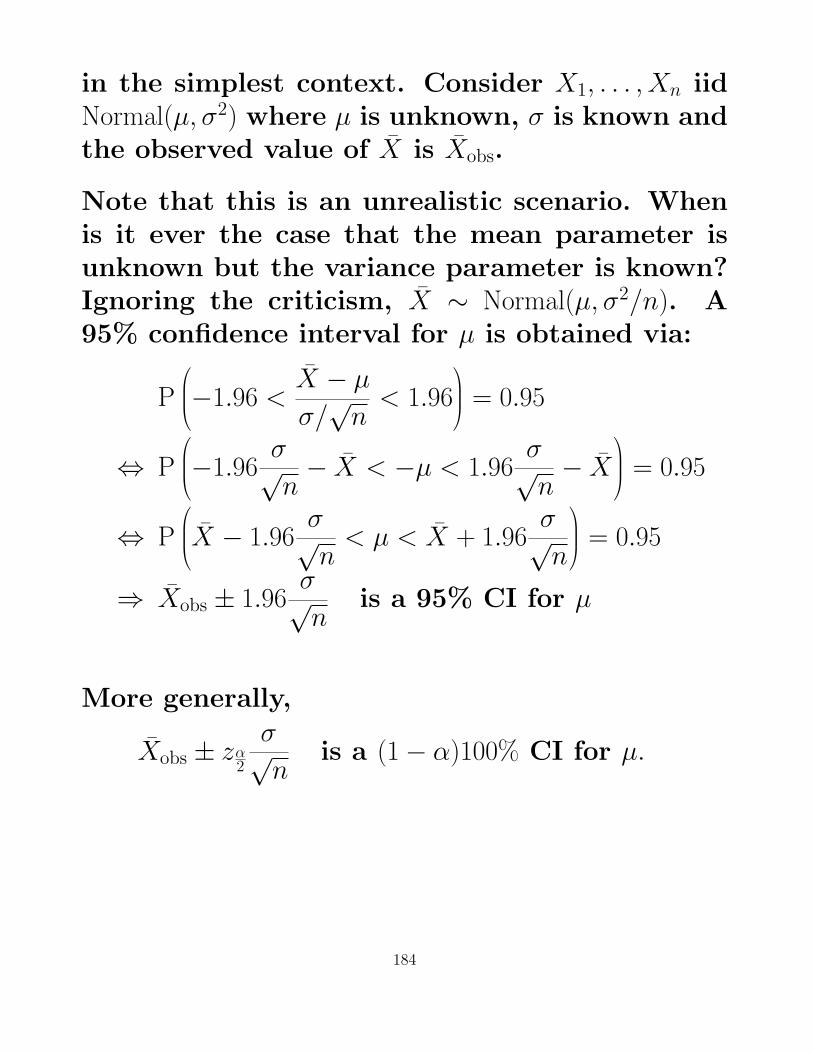
in the simplest context. Consider X1, . . . , Xn iidNormal(µ, σ2) where µ is unknown, σ is known andthe observed value of X is Xobs.
Note that this is an unrealistic scenario. Whenis it ever the case that the mean parameter isunknown but the variance parameter is known?Ignoring the criticism, X ∼ Normal(µ, σ2/n). A95% confidence interval for µ is obtained via:
P
−1.96 <X − µσ/√n< 1.96
= 0.95
⇔ P
−1.96σ√n− X < −µ < 1.96
σ√n− X
= 0.95
⇔ P
X − 1.96σ√n< µ < X + 1.96
σ√n
= 0.95
⇒ Xobs ± 1.96σ√n
is a 95% CI for µ
More generally,
Xobs ± zα2σ√n
is a (1− α)100% CI for µ.
184

Interpretation of CI’s: The explanation is subtleand you need to pay close attention.
Consider many hypothetical replications of anexperiment.
A common but incorrect interpretation for CI’S:
If Xobs±zα2σ√n is a (1−α)100% CI for µ, it is incorrect
to write P(µ ∈ Xobs ± zα2
σ√n
)= 1− α.
185

Discussion points wrt the CI Xobs ± zα2σ√n:
• as n increases, the width of the CI decreases
• as our confidence increases (ie. 1− α bigger),the width of the CI increases
• tradeoff: we want narrow CI’s with large con-fidence
• a CI of a given confidence 1− α is not unique
186

The simple but unrealistic CI setting previouslypresented is extended to more realistic scenarios.
We begin by assuming that our sample X1, . . . , Xn
is large (ie. n ≥ 30) as is often the case in practice.
Case 1: Since n is large, we can invoke the CLTwhere approximately X ∼ Normal(µ, σ2/n). Whatis great about this is that we no longer need toassume that the X’s are normal. In this case,
Xobs ± zα2σ√n
is an approximate (1−α)100% CI for µ where σ isstill assumed known.
Case 2: We have the same conditions as Case 1except that σ is unknown. In this realistic case,
Xobs ± zα2s√n
is an approximate (1−α)100% CI for µ where s isthe sample standard deviation.
187

Example: Consider heat measurements taken indegrees Celsius where µ = 5 and σ = 4. A changeis made in the process such that µ changes butσ remains the same. We observe Xobs = 6.1 basedon n = 100 observations.
(a) Construct a 90% CI for µ.
(b) How big should the sample size be such thatthe CI is less than 0.6 degrees wide?
188

Problem: Consider the CI Xobs ± zα2σ√n.
(a) How much should the sample size n increaseto reduce the width of by half?
(b) What is the effect of increasing the samplesize by a factor of 25?
189

Lecture 27
We now construct a confidence interval for theunknown p in the model X ∼ Binomial(n, p). Werequire np ≥ 5 and n(1− p) ≥ 5 (ie. n large and pmoderate) so that we can use the approximationX ∼ Normal(np, np(1− p)). We denote p = X/n andpobs = Xobs/n. A (1−α)% confidence interval for pis obtained via:
P
−zα2<
X − np√np(1− p)
< zα2
= 1− α
⇔ P
−zα2<
p− p√p(1− p)/n
< zα2
= 1− α
⇔ P(−zα
2
√p(1− p)/n− p < −p < zα
2
√p(1− p)/n− p
)= 1− α
⇔ P(p− zα
2
√p(1− p)/n < p < p + zα
2
√p(1− p)/n
)= 1− α
Therefore,
pobs ± zα2√pobs(1− pobs)/n (1)
is an approximate (1 − α)100% CI for p. The CI(1) is based on two approximations:
1. approximating the Binomial with the Normal
2. replacing p with p
190

Example: From a sample of 1250 BC voters, 420indicate that they support the NDP. Obtain anapproximate 95% CI for the proportion of BCvoters who support the NDP.
191

CI’s based on the Student distribution: SupposeX1, . . . , Xn are iid Normal(µ, σ2) where σ is unknown(the realistic case). It can be shown that
X − µs/√n∼ tn−1
where tn−1 denotes the t distribution with n − 1degrees of freedom. The pdf of Y ∼ tn−1 is
f (y) =Γ(n/2)
Γ((n− 1)/2)Γ(1/2)
1 +y2
n− 1
−n/2
Here, the (1−α)100% confidence interval for µ is
X ± tα2 ,n−1
s√n
Discussion points:
• the tn−1 distribution is symmetric on R• the tn−1 has longer tails than the normal
• as n→∞, tn−1 → Z ∼ Normal(0, 1)
• for n ≥ 30, you can replace tn−1 with Z
• the t distribution is intractable; no need tomemorize pdf
• Table B.1 in the text gives points tα2 ,n−1
192

The logic of hypothesis testing: We view thetesting of hypotheses as consisting of three steps.We discuss the three steps in some detail.
1. The experimenter forms a null hypothesis H0
to test against an alternative hypothesis H1.
2. The experimenter collects data.
3. In the inference step, the question is asked“Are the data compatible wrt H0?” If yes, H0
is not rejected. If no, H0 is rejected.
193

Example: In this informal example, we go overthe three steps of hypothesis testing. Imagine acourt of law where a defendent is accused of acrime.
194

Example: In this informal example, we go overthe three steps of hypothesis testing. Imaginethat you are playing cards and that your friendhas obtained a royal flush three hands in a row.
195

In the inference step, if we answer “yes” to thekey question (Are the data compatible wrt H0?),we conclude using the curious language, “H0 isnot rejected”. We discuss why this does notmean the same thing as “H0 is accepted”.
196

Lecture 28
In this lecture, we examine five examples eachof which does something different in the contextof hypothesis testing.
To address the inference step (step 3 of hypoth-esis testing), we compute a p-value which is de-fined as the probability of observing a result asextreme or more extreme than what we observedgiven that H0 is true (think about this!)
The convention is to reject H0 and conclude H1
if the p-value is less than 0.05. Sometimes astronger level of evidence is required (e.g. 0.01).
197

Example: A shop sells coffee where the numberof lb of coffee sold in a week is Normal(320, 402).After advertising, 350 lb is sold in the followingweek. Has advertising improved business?
198

Example: A soup company makes soup in 10 ozcans. A sample of 48 cans has mean volume 9.82oz and s = 0.8 oz. Can we conclude that the com-pany is cheating? Test at level 0.01 significance.
199

Example: A coin is flipped 10 times and 8 headsappear. Is the coin fair?
200

Example: A coin is flipped 100 times and 60heads appear. Is the coin fair?
201

Example: A paint is applied to tin panels andbaked for one hour such that the mean index ofhardness is 35.2. Suppose 20 panels are paintedand baked for three hours, and their sample meanindex of hardness is 37.2 with s = 1.4. Does bak-ing for three hours strengthen panels? Assumenormal data.
202

Single Sample Testing - Summary
Data Test Statistic Comments
normal, X−µσ/√n ∼ N(0, 1) unrealistic
σ known
normal, X−µs/√n ∼ tn−1 N(0,1) when n ≥ 30
σ unknown
non-specified, X−µσ/√n ∼ N(0, 1) unrealistic
σ known, based on CLTn ≥ 30
non-specified, X−µs/√n ∼ N(0, 1) based on CLT
σ unknown,n ≥ 30Binomial Binomial
Binomial, p−p√p(1−p)/n
∼ N(0, 1)
np ≥ 5,n(1− p) ≥ 5
203

Lecture 29
We now study the two sample problem where thedata X1, . . . , Xm iid Normal(µ1, σ
21) is independent of
Y1, . . . , Yn iid Normal(µ2, σ22). Initially, we make the
unrealistic assumption that both σ1 and σ2 areknown.
Under the above conditions, interest lies in theunknown parameter µ1 − µ2. The test statisticused in the construction of confidence intervalsand hypothesis testing is
X − Y − (µ1 − µ2)√σ2
1/m + σ22/n
∼ Normal(0, 1)
204

Example: Suppose that fifty test scores fromclass A are independent of 70 test scores fromclass B. Assume further that the test scores arenormal, σ2
1 = σ22 = 84, X = 73 and Y = 59. Is there
a difference between the two classes?
205

Example continued: Construct a 95% confidenceinterval for µ1 − µ2.
Example continued: Suppose the question hadinstead been, “Is class A better than class B?”
206

Example continued: Suppose the question hadinstead been, “Is class A more than five marksbetter than class B?”
207

The significance of ”significance”:
When we reject the null hypothesis H0, we saythat the result is statistically significant.
Discussion points:
• always report the p-value
• keep in mind that α = 0.05 is arbitrary
• significance does not always mean importance
• p-values are related to sample size
208

More on stat significance vs practical importance:
Example: Spring Birthday Confers Height Ad-vantage - Yahoo Health News, Feb 18/98
In an Austrian study of 507,125 military recruits,it was found that the average height of thoseborn in the spring was 1/4 inch more than thoseborn in the fall.
209
Lecture 30
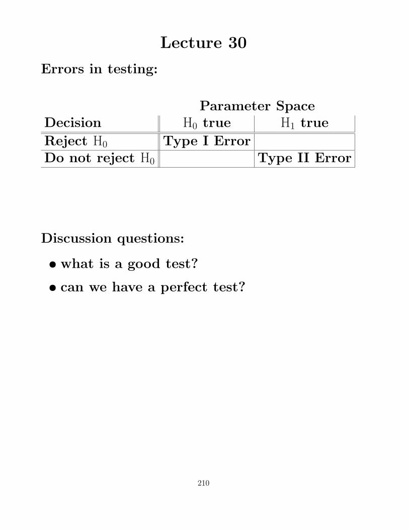
Errors in testing:
Parameter SpaceDecision H0 true H1 true
Reject H0 Type I ErrorDo not reject H0 Type II Error
Discussion questions:
• what is a good test?
• can we have a perfect test?
210

Example: We examine Type I error and Type IIerror in the earlier example where a defendentis accused of a crime in a court of law.
211

Probabilities associated with errors in testing:
Parameter SpaceDecision H0 true H1 true
Reject H0 α 1− βDo not reject H0 β
Discussion points:
• α is the significance level of a test
• we typically fix α
• 1− β is referred to as the power of a test
• we want the power to be large
• α, β are test properties; indpt of data
• note that in our examples, H0 is simple
• note that in our examples, H1 is composite
212

Example: We return to the one sample problemwhere X1, . . . , Xn are iid, σ = 1.8, α = 0.05 andn = 100. We are interested in testing H0 : µ = 3versus H1 : µ > 3.
(a) Find the critical region (rejection region).
(b) Calculate the power at µ = 3.2.
(c) Calculate the power at µ = 3.5.
(d) What happens in (b) when n = 100→ 400?
213
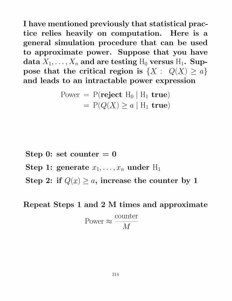
I have mentioned previously that statistical prac-tice relies heavily on computation. Here is ageneral simulation procedure that can be usedto approximate power. Suppose that you havedata X1, . . . , Xn and are testing H0 versus H1. Sup-pose that the critical region is {X : Q(X) ≥ a}and leads to an intractable power expression
Power = P(reject H0 | H1 true)
= P(Q(X) ≥ a | H1 true)
Step 0: set counter = 0
Step 1: generate x1, . . . , xn under H1
Step 2: if Q(x) ≥ a, increase the counter by 1
Repeat Steps 1 and 2 M times and approximate
Power ≈ counter
M
214

Lecture 31
Example: Consider X ∼ Bin(500, p) where we testH0 : p = 0.7 versus H1 : p 6= 0.7 at level α = 0.01.
(a) Find the critical region of the test.
(b) Calculate the power at p = 0.6.
215

Example: In a two sample test of H0 : µ1 − µ2 = 3versus H1 : µ1 − µ2 > 3, suppose that the dataare normal, m = n and σ2
1 = σ22 = 84.0. Can we
choose m such that the test has level α = 0.01 andβ = 0.05 at µ1 − µ2 = 5.0? This question concernsexperimental design.
216

In two sample problems, we can relax the nor-mality assumption in the case of large samples.
Given X1, . . . , Xm iid independent of Y1, . . . Yn iidwith m and n large (ie. m,n ≥ 30), then the fol-lowing statistic can be used for testing and theconstruction of confidence intervals.
X − Y − (µ1 − µ2)√s2
1/m + s22/n
∼ Normal(0, 1)
where µ1 and µ2 are the respective means, and s1
and s2 are the respective sample std devs.
217

Example: A college interviewed 1296 studentswrt summer incomes. Based on the results in thefollowing table, test whether there is a differencein earnings between male and female students.
Students n X smale 675 $1884.52 $1368.37female 621 $1360.39 $1037.46
218

Example: The test scores of first year studentsadmitted to college directly from high school his-torically exceed the test scores of first year stu-dents with working experience by 10%. A recentsample of 50 first year students admitted directlyfrom high school has an average test score of74.1% with std dev 3.8%. An indpt sample of50 first year students with working experienceyields an average test score of 66.5% with stddev 4.1%. Test whether a change has occurred.
219

Lecture 32
We consider another variation to the two sampleproblem. This time, the data are again normal.Realistically, σ1 and σ2 are unknown but we needto make the additional assumption σ1 = σ2.
Given X1, . . . , Xm iid Normal(µ1, σ21) independent of
Y1, . . . Yn iid Normal(µ2, σ22) with σ1 = σ2, then the
following statistic can be used for testing andthe construction of confidence intervals.
X − Y − (µ1 − µ2)√√√√( 1m + 1
n
) (m−1)s21+(n−1)s2
2m+n−2
∼ tm+n−2
where s1 and s2 are the respective sample stddevs.
220

Example: The Chapin Social Insight Test gavethe following scores. Assuming normal data, testwhether the mean score of males exceeds themean score of females.
Group n X smales 18 25.34 13.36females 23 24.94 14.39
221

Example cont’d: Obtain a 95% CI for µ1 − µ2.
222

There are actually lots of testing methodologiescorresponding to different data scenarios. Wewill study one more situation (a common oneinvolving paired data) but keep in mind thatthe principles that we have studied carry overto more complex situations.
Suppose in the paired data situation, we haveX1, . . . , Xn iid arising from a population with meanµ1, and Y1, . . . , Yn iid arising from a populationwith mean µ2. Furthermore, assume that thedata are paired such that Xi corresponds to Yi.This natural pairing implies that there is a de-pendence between Xi and Yi.
To carry out inference (testing and the construc-tion of CI’s), we define a new random variable,the difference Di = Xi−Yi. Our interest concernsthe unknown parameter
E(Di) = E(Xi − Yi)= E(Xi)− E(Yi)
= µ1 − µ2.
Our analysis proceeds as in the single samplecase based on the data D1, . . . , Dn.
223

Example: Suppose scores measuring jitterinessare normally distributed . We believe that scoresincrease after drinking coffee. Let Xi be the be-fore drinking coffee score and let Yi be the theafter drinking coffee score for the i-th individual.Based on α = 0.01, test the hypothesis.
xi yi di50 5660 7055 6072 7085 8278 8465 6890 88
224

Example cont’d: Obtain a 95% CI for the meandifference in jitteriness scores.
225

Example cont’d: Suppose we have the same databut the experiment involves 16 people where 8people were measured without having coffee and8 other people where measured after drinkingcoffee. How does the analysis differ?
226

Example cont’d: Suppose now that the 16 peopleinvolve 8 pairs of twins such that Xi and Yi aretwins. How should the analysis proceed?
Example cont’d: Assume the same conditions asabove but the data are no longer normal. Howshould the analysis proceed?
227

Pairing is a special case of blocking (read in text).Blocking attempts to reduce variation by group-ing data that are similar, and this hopefully leadsto more sensitive tests (ie. tests that reject H0
more often when H0 is false).
Example: To illustrate the above, consider fivebefore and after measurements involving a drugwhere there are big differences in responses be-tween people but there is small variation in theDi’s. Assuming normal data, we carry out apaired analysis and a non-paired analysis.
xi yi di25 29 −446 50 −430 33 −375 78 −319 25 −6
228

Two Sample Testing - Summary
Assume X1, . . . , Xm iid with mean µ1 and std devσ1, and Y1, . . . , Yn iid with mean µ2 and std dev σ2.
Data Test Statistic Comments
paired data, take Di = Xi − Yi andm = n refer to single sample case
non-paired, X−Y−(µ1−µ2)√σ2
1/m+σ22/n∼ N(0, 1) replace σi’s with si’s
m,n large if σi’s unknown
non-paired, X−Y−(µ1−µ2)√σ2
1/m+σ22/n∼ N(0, 1) unrealistic
m,n not large,data normal,σi’s known
non-paired, X−Y−(µ1−µ2)√( 1
m+ 1n)s2p
∼ tm+n−2 s2p = (m−1)s21+(n−1)s22
m+n−2
m,n not large,data normal,σ1 ≈ σ2
but unknown
binomial data, p1−p2−(p1−p2)√p1(1−p1)/m+p2(1−p2)/n
∼ normal(0, 1) replace p’s with estimates
m,n large, in denominatorp1, p2 moderate
229


