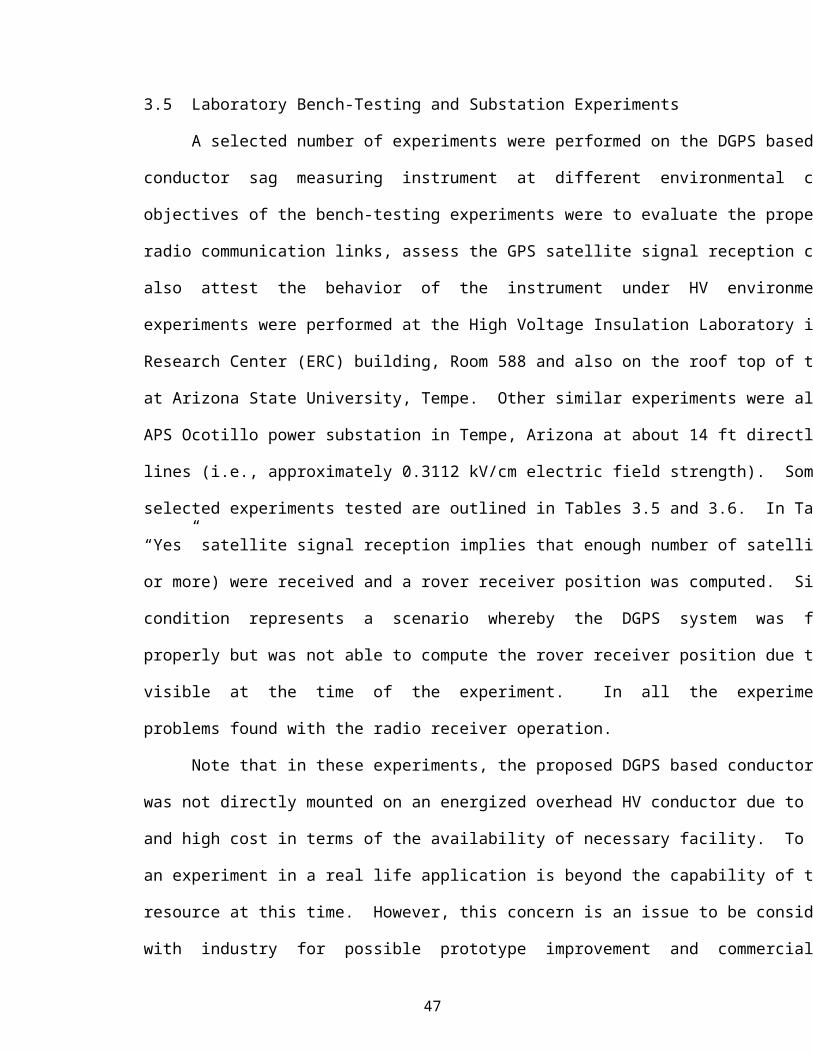
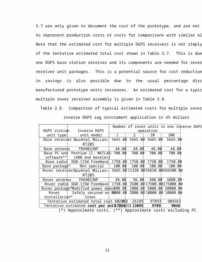
1 Arizona State University Entergy Arizona Public Service INSTRUMENTATION AND MEASUREMENT OF OVERHEAD CONDUCTOR SAG USING THE DIFFERENTIAL GLOBAL POSITIONING SATELLITE SYSTEM Chris Mensah-Bonsu August, 2000
Transcript
1
Arizona State University Entergy Arizona Public Service
INSTRUMENTATION AND MEASUREMENT OF
OVERHEAD CONDUCTOR SAG USING THE
DIFFERENTIAL GLOBAL POSITIONING SATELLITE
SYSTEM
Chris Mensah-Bonsu
August, 2000
2
This is a reproduction of a PhD thesis of Dr. Chris Mensah Bonsu of the
California ISO. Dr. Mensah Bonsu completed this work in August, 2000. The work was
supported by a Power Systems Engineering Research Center (PSerc) project under the
sponsorship of Entergy and Arizona Public Service. Dr. G. T. Heydt was the project
principal investigator and Dr. Mensah Bonsu's advisor.
3
ABSTRACT
This dissertation work deals with the design, construction, instrumentation and
testing of a differential global positioning satellite (DGPS) system based instrument for the
measurement of overhead high voltage (HV) conductor sag. Inherent and intentional errors
in GPS technologies are discussed, and the DGPS method is described for accuracy
enhancement. A DGPS based overhead conductor sag measuring instrument has been
designed, constructed and subjected to selected laboratory bench and power substation
testing. A method to directly measure the physical sag of overhead HV conductors is
described. The main advantage of the concept is the real time direct measurement of a
parameter (i.e., conductor sag) needed for the operation of the transmission system without
intermediate measurement of conductor tension, temperature, and ambient weather
conditions. A further potential advantage is cheaper cost. The main objectives of the
experimental tests conducted were to evaluate the proper functioning of the radio
communication links, assess the DGPS receiver capability in terms of GPS signal
reception, and to also attest the behavior of the conductor sag measuring instrument under
HV environment.
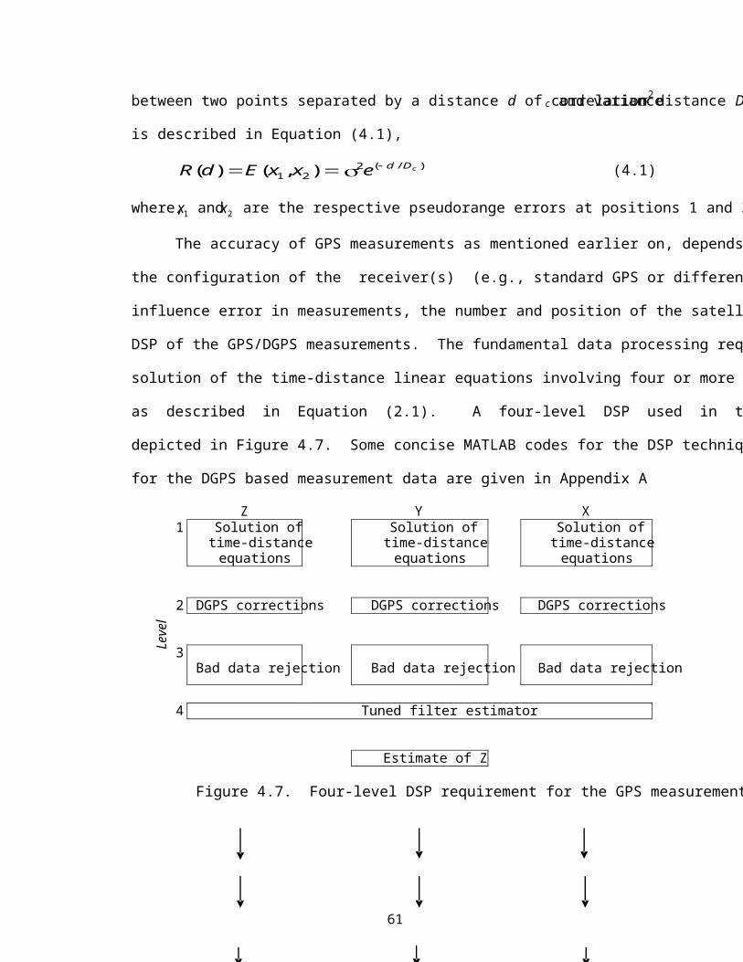
A digital signal processing (DSP) methodology to further improve the DGPS based
altitude measurements for overhead conductor sag is described in detail in a four-level
configuration. This involves data processing that is needed to attenuate noise levels and to
enhance the measurement accuracy. The methods of bad data identification and
modification, least squares parameter estimation, artificial neural network, and Haar
wavelet transform analysis have been utilized to further reduce the error of raw DGPS
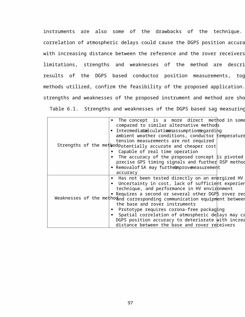
measurements significantly. Typical accuracy, response time, strengths and weaknesses
4
of the instrument and method are also described. An outline of a methodology to integrate
the resulting real time direct overhead conductor sag measurement data with dynamic
thermal line rating (DTLR) is also described.
Experience in many electric utility industries shows that the clearance of an
overhead (HV) conductor above ground is a key factor limiting the available transfer
capacity (ATC) of the conductor, especially in regions of high interconnection. Hence, the
pertinence of conductor sag measurement to circuit operation relates to the calculation of
DTLR. Thus, power systems operation and reliability could be improved by continuously
monitoring the physical overhead HV conductor sag. To be able to rapidly and accurately
determine the DTLR of a circuit has obvious pecuniary value in the open access same time
information system (OASIS). Ultimately, the results obtained in this respect for a given
operating condition could be used for anticipatory system loading purposes.
5
DEDICATION
To my mother, Ama Konadu (“ baa tan pa”) of Adjamesu in Amansie, Ashanti
and also, to the memory of my grandmother - Nana Afua Dufie, I thank for everything.
6
ACKNOWLEDGEMENTS
First and foremost, I thank God, the Almighty for his strength and blessings. I
would like to thank Dr. Gerald T. Heydt for the opportunity to work with him, and also for
his encouragement, trust and untiring support. Dr. Heydt has been an advisor in the true
sense both academically and morally throughout this work. It is my fervent hope that our
treasured friendship continues to enjoy progressively seamless growth.
It is a pleasure to acknowledge the following individuals who have contributed to,
and influenced this work: John Schilleci, Douglas A. Selin, Dr. Baj Agrawal, and Dr.
George G. Karady. Prof. Richard G. Farmer, who is also one of my committee members,
provided substantive insight on dynamic thermal line ratings and the research work as a
whole. I also appreciate the efforts and comments from my committee members: Dr. Ravi
S. Gorur, Dr. Keith E. Holbert, and Dr. Elizabeth K. Burns. The contributions of Joshua
A. Burns, Duane R. Torgeson and John A. Demcko are also acknowledged. I am grateful
to the following students: John S. Wells, Yuri Hoverson and Ubaldo Fernández Krekeler
whose diverse assistance in this work deserve a special recognition. Alex Hunt and Trevor
Yancey are also acknowledged for their contributions in providing an initial prototype
instrument on which a main concept of the dissertation is based.
Thanks to the Department of Electrical Engineering and the College of Engineering
and Applied Sciences at Arizona State University (ASU), Arizona Public Service, Entergy,
and the National Science Foundation Center for the Advanced Control of Energy and
Power Systems/Power Systems Engineering Research Center (ACEPS/PSERC), whose
generous sponsorship made this work possible. The generosity of Rick Faulkner, Andy
Carbognin and the staff at NovAtel Inc., Calgary, Canada and the initial loan of OEM3-
7
3111R DGPS receivers were critical to this work, and so are the initial loan of the
FreeWaveTM DGR-115 W spread spectrum radio modems from Steve Meier and Michael
Brown of Steve Lieber and Associates, Inc. Webster, Texas.
Furthermore, my gratitude to all those people who have helped to bring me to this
stage of my career. My parents, family and fiancée (Patti) for the much needed moral
support and loving kindness, and also to my elementary school teachers: Alexander A.
Addison and Rose A. Apraku for their good initial nursing in my academic endeavor. Last
but not the least, my sincere gratitude goes to the administrative personnel of the ASU
Department of Electrical Engineering: Ms. Darleen E. Mandt, Ms. Virginia L. Cruz, and
also all the graduate research students in the Power Engineering Program at ASU for their
numerous assistance and the wonderful moments we shared together. It is impossible to
mention everyone who has contributed ideas, suggestions, concepts and also supported me
in diverse ways, but I owe you all my deepest thanks.
8
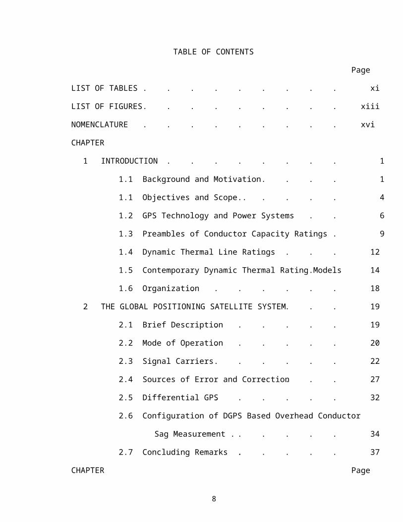
TABLE OF CONTENTS
Page
LIST OF TABLES . . . . . . . . . xi
LIST OF FIGURES . . . . . . . . . xiii
NOMENCLATURE . . . . . . . . . xvi
CHAPTER
1 INTRODUCTION . . . . . . . . 1
1.1 Background and Motivation . . . . . 1
1.1 Objectives and Scope . . . . . . 4
1.2 GPS Technology and Power Systems . . . 6
1.3 Preambles of Conductor Capacity Ratings . . . 9
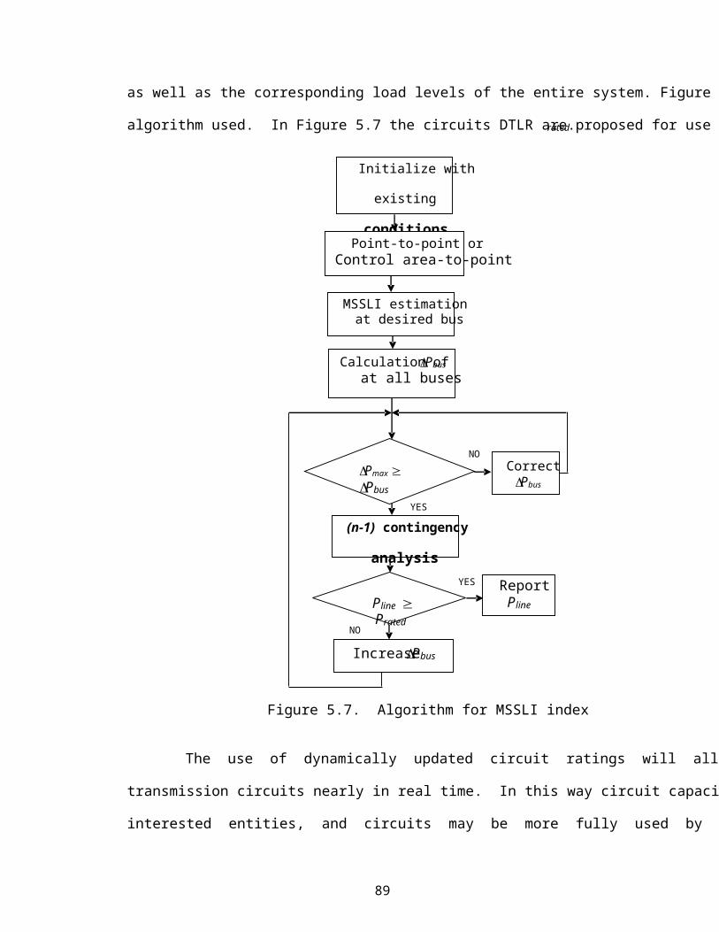
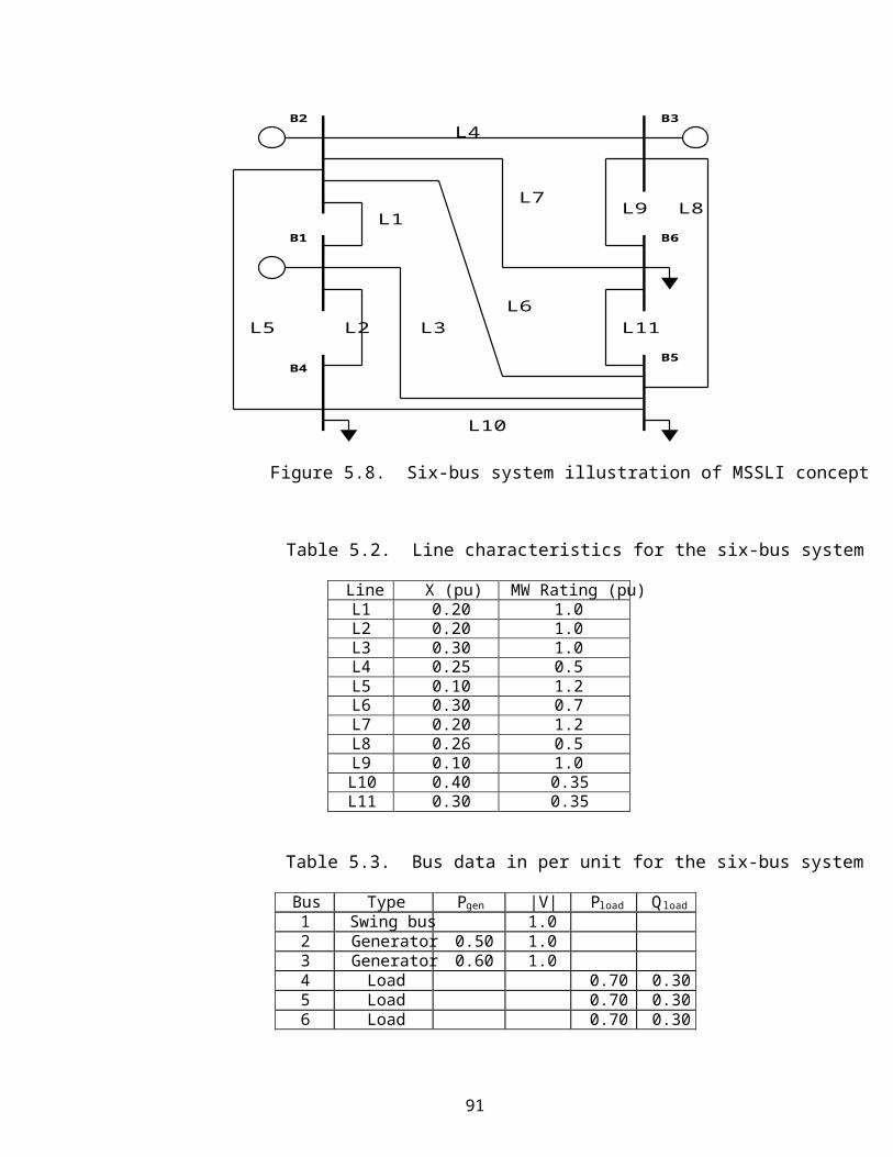
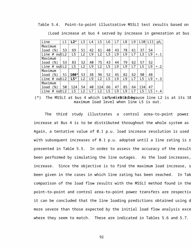
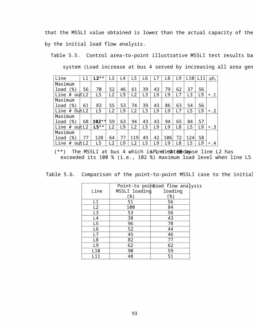
5.8 Six-bus system illustration of MSSLI concept . . . . 91
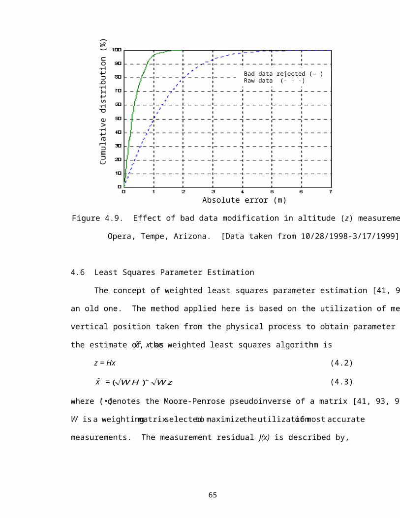
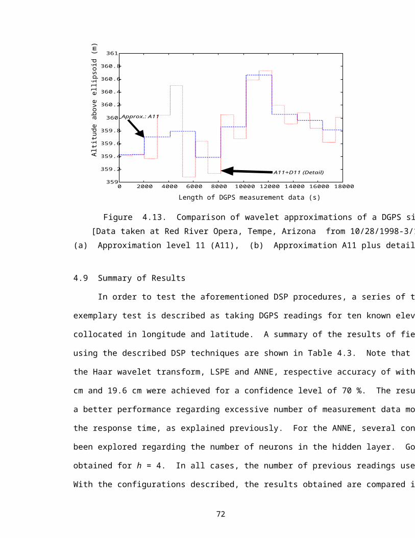
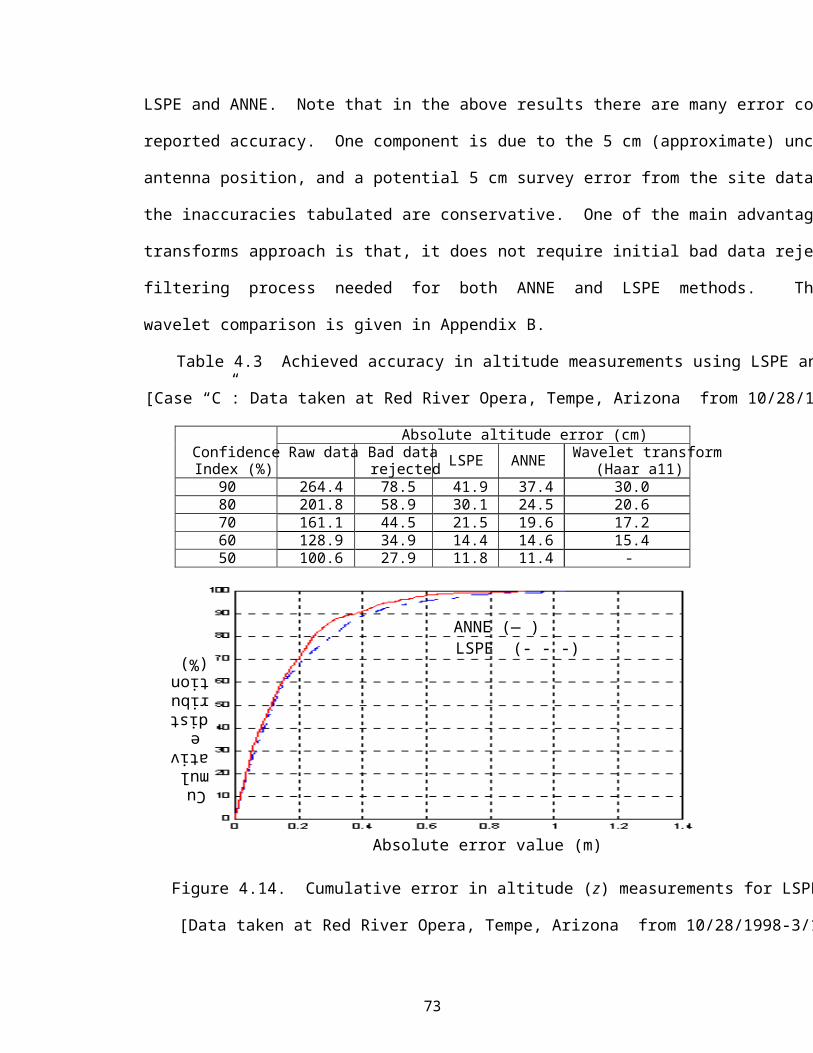
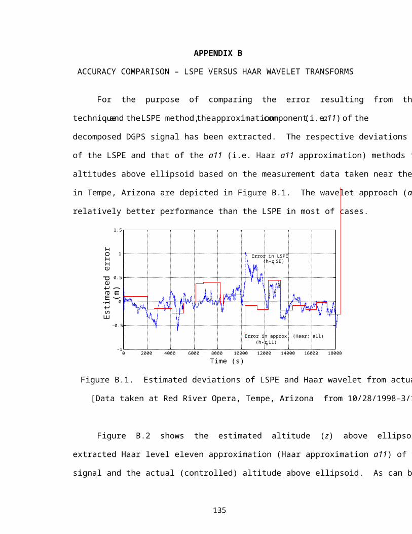
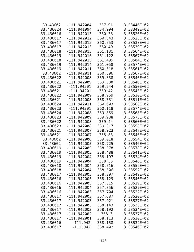
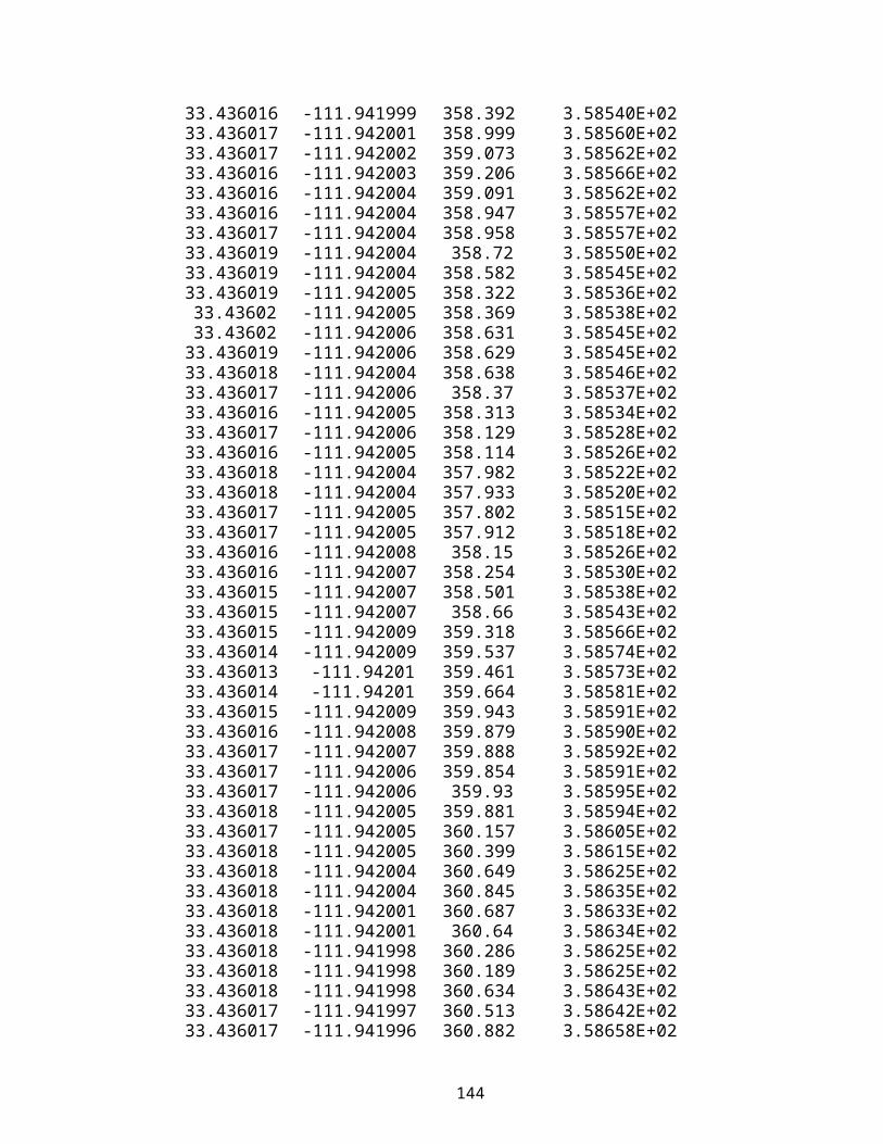
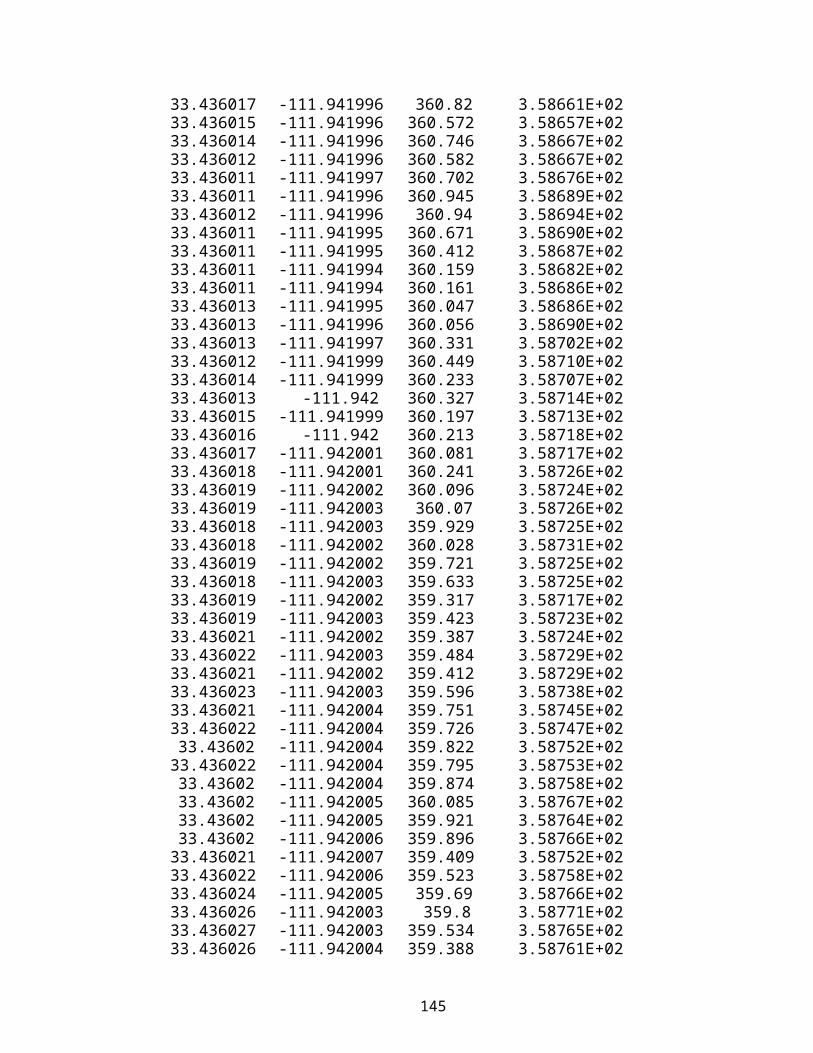
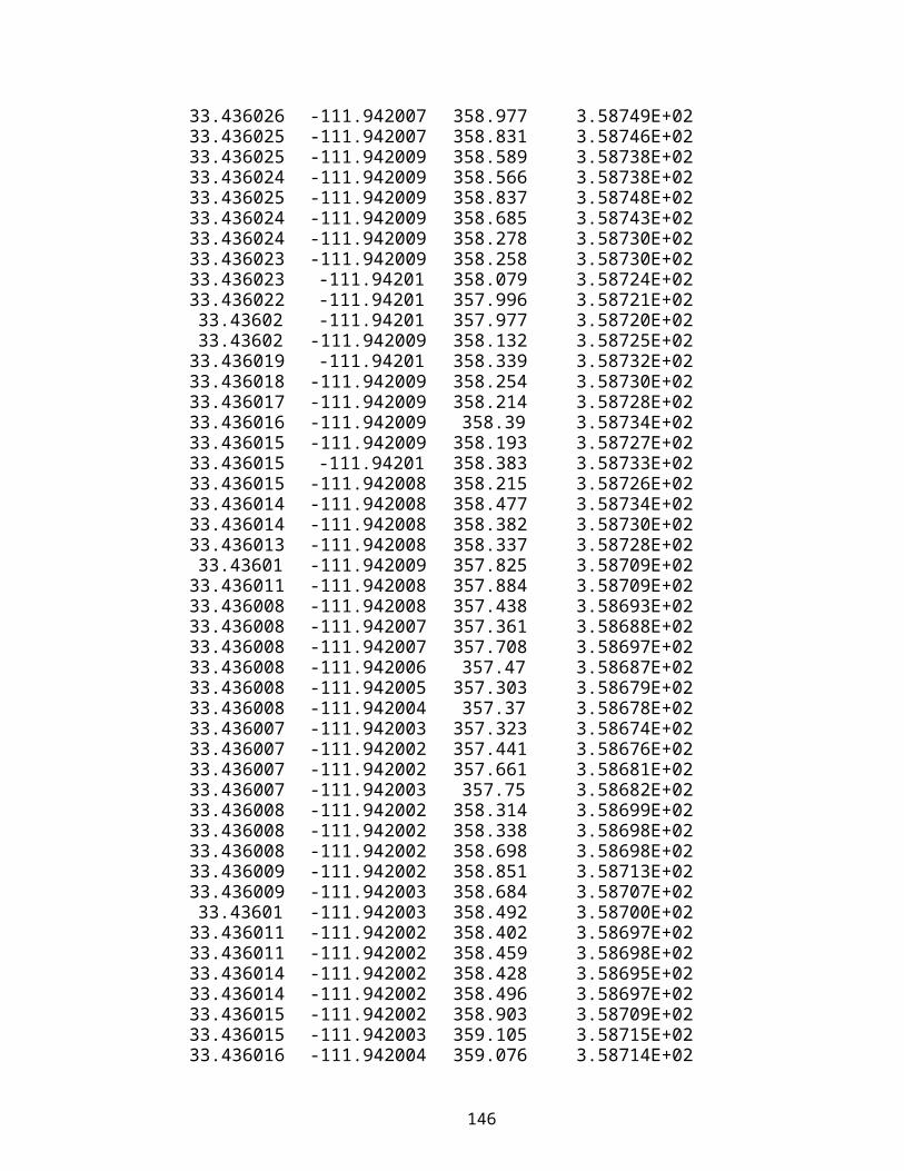
B.1 Estimated deviations of LSPE and Haar wavelet from actual altitudes (z)
[Data taken at Red River Opera, Tempe, Arizona
from 10/28/1998-3/17/1999] . . . . . . 138
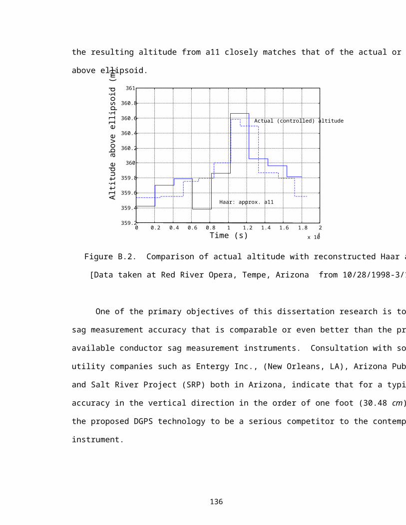
B.2 Comparison of actual altitude with reconstructed Haar approximation
[Data taken at Red River Opera, Tempe, Arizona
from 10/28/1998-3/17/1999] . . . . . . 139
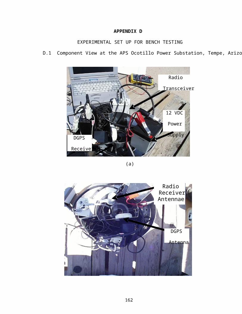
D. 1 Bench testing set up of the integrated DGPS rover unit . . . 164
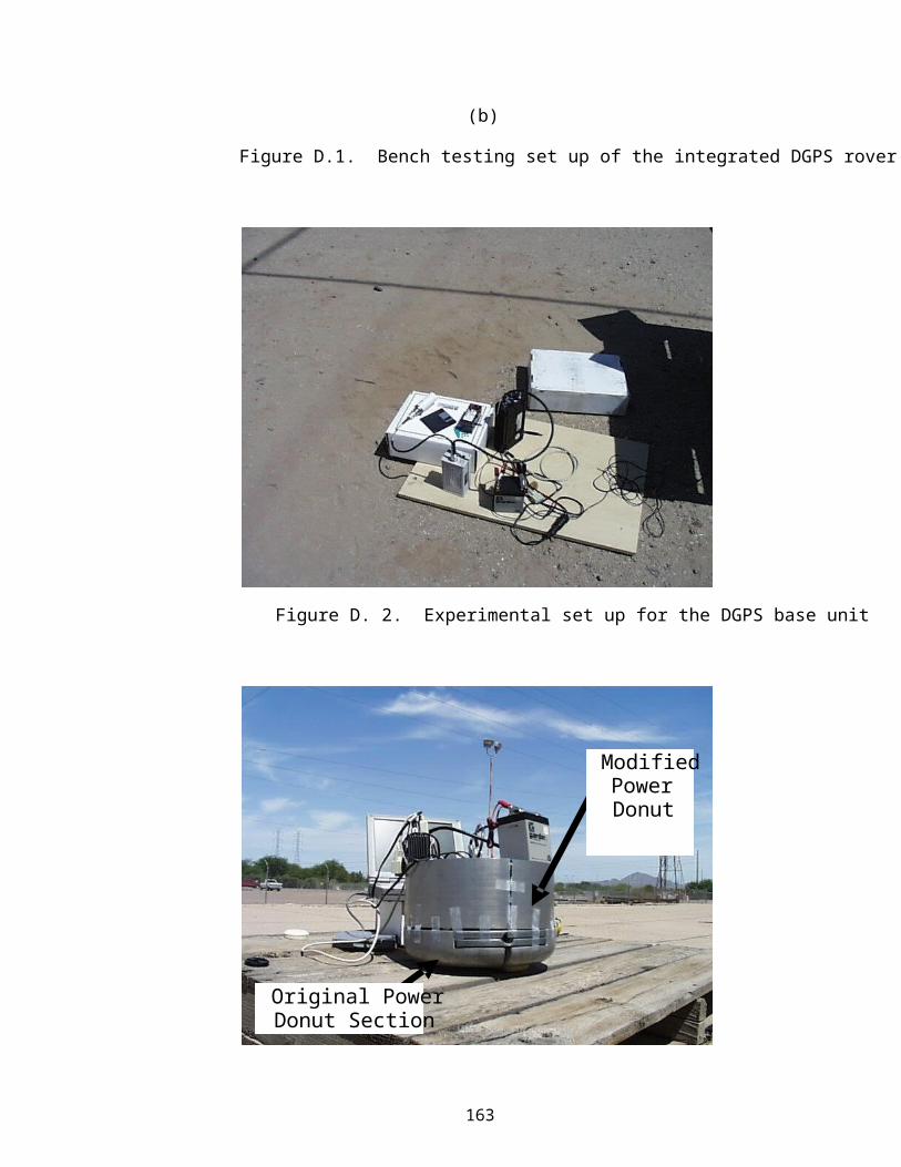
D. 2 Experimental set up for the DGPS base unit . . . . . 165
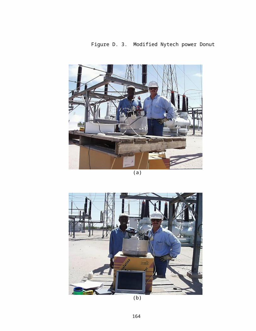
D. 3 Modified Nytech Power Donut . . . . . . 165
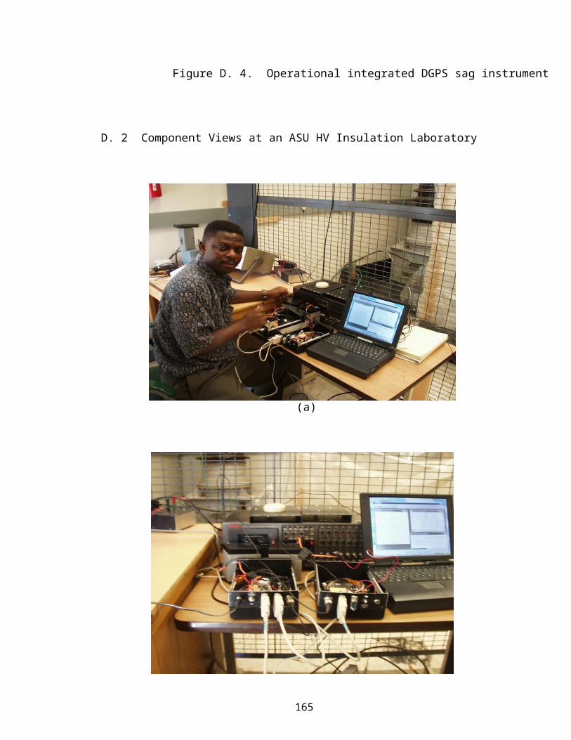
D. 4 Operational integrated DGPS sag instrument . . . . . 166
D. 5 Indoor experimental set up in the ERC building . . . . 167
16
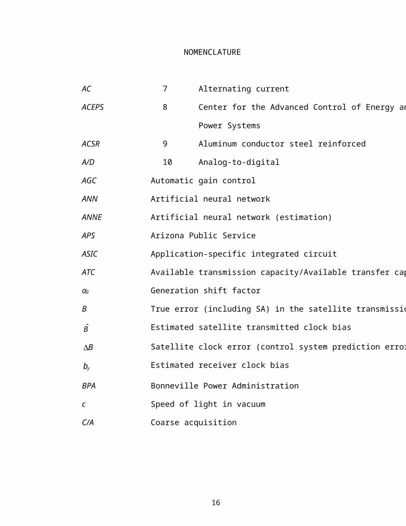
NOMENCLATURE
AC 7 Alternating current
ACEPS 8 Center for the Advanced Control of Energy and
Power Systems
ACSR 9 Aluminum conductor steel reinforced
A/D 10 Analog-to-digital
AGC Automatic gain control
ANN Artificial neural network
ANNE Artificial neural network (estimation)
APS Arizona Public Service
ASIC Application-specific integrated circuit
ATC Available transmission capacity/Available transfer capability
ali Generation shift factor
B True error (including SA) in the satellite transmission time
B Estimated satellite transmitted clock bias
B Satellite clock error (control system prediction error)
rb Estimated receiver clock bias
BPA Bonneville Power Administration
c Speed of light in vacuum
C/A Coarse acquisition
17
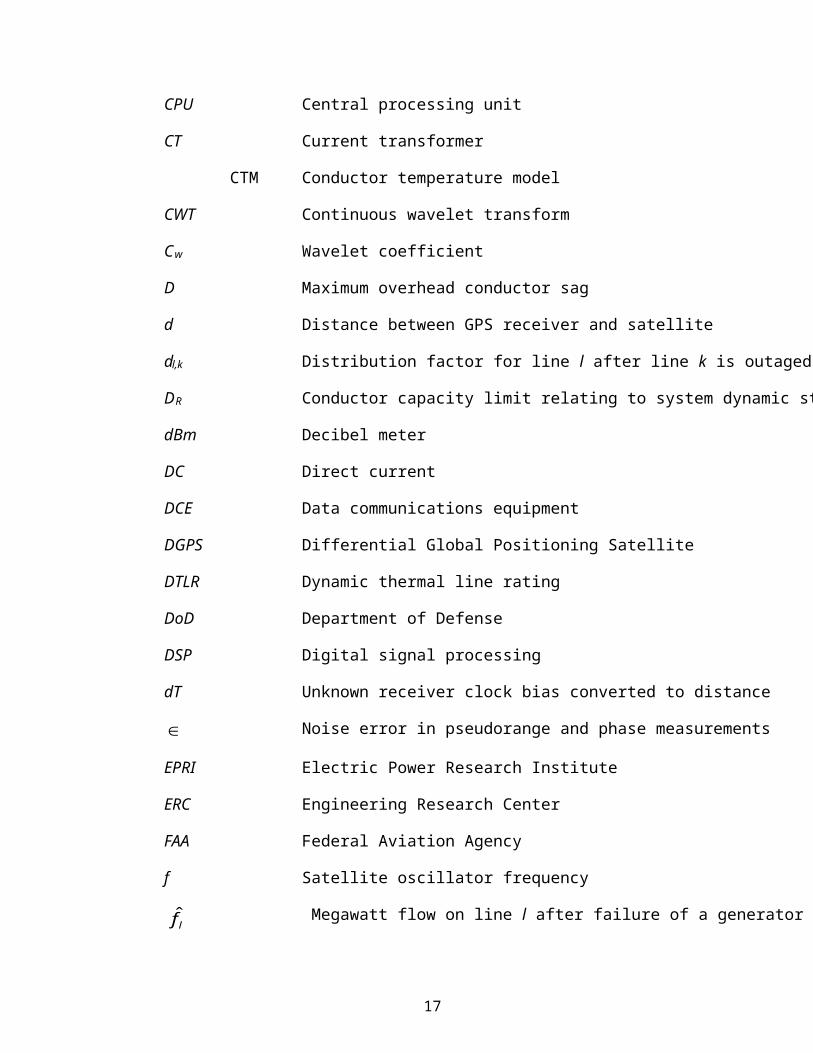
CPU Central processing unit
CT Current transformer
CTM Conductor temperature model
CWT Continuous wavelet transform
Cw Wavelet coefficient
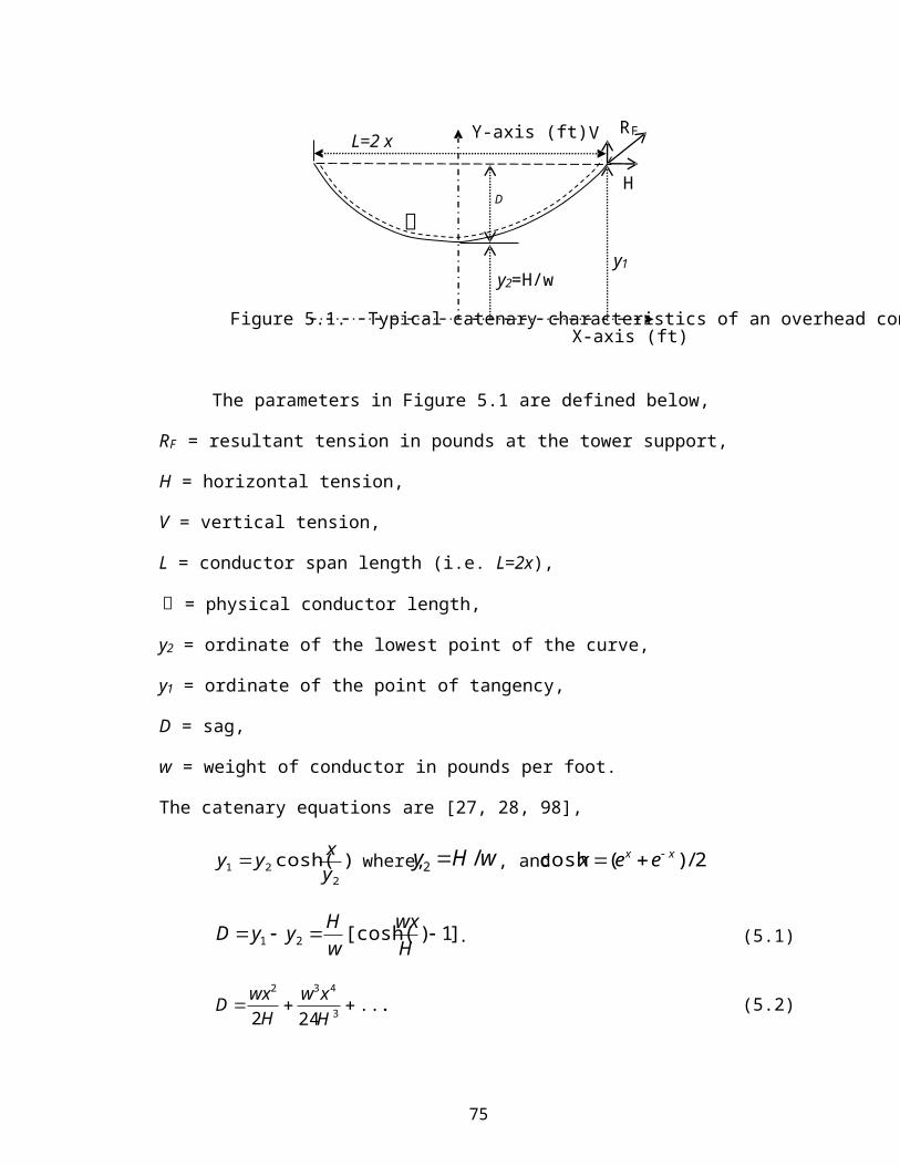
D Maximum overhead conductor sag
d Distance between GPS receiver and satellite
dl,k Distribution factor for line l after line k is outaged
DR Conductor capacity limit relating to system dynamic state response
dBm Decibel meter
DC Direct current
DCE Data communications equipment
DGPS Differential Global Positioning Satellite
DTLR Dynamic thermal line rating
DoD Department of Defense
DSP Digital signal processing
dT Unknown receiver clock bias converted to distance
Noise error in pseudorange and phase measurements
EPRI Electric Power Research Institute
ERC Engineering Research Center
FAA Federal Aviation Agency
f Satellite oscillator frequency
lf Megawatt flow on line l after failure of a generator on bus i
18
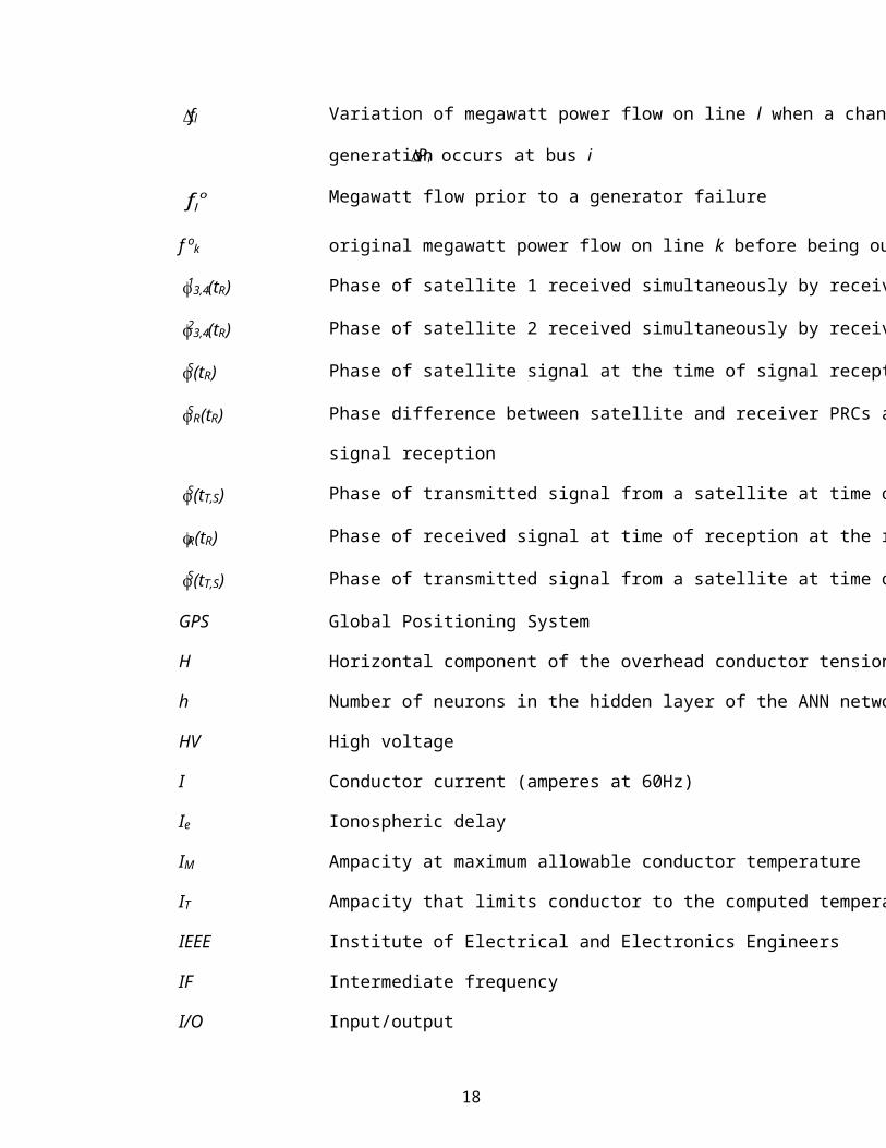
fl Variation of megawatt power flow on line l when a change in
generation Pi occurs at bus i
olf Megawatt flow prior to a generator failure
f ok original megawatt power flow on line k before being outaged
13,4(tR) Phase of satellite 1 received simultaneously by receivers 3 and 4
23,4(tR) Phase of satellite 2 received simultaneously by receivers 3 and 4
S(tR) Phase of satellite signal at the time of signal reception at a receiver
SR(tR) Phase difference between satellite and receiver PRCs at time of
signal reception
S(tT,S) Phase of transmitted signal from a satellite at time of transmission
R(tR) Phase of received signal at time of reception at the receiver
S(tT,S) Phase of transmitted signal from a satellite at time of transmission
GPS Global Positioning System
H Horizontal component of the overhead conductor tension
h Number of neurons in the hidden layer of the ANN network
HV High voltage
I Conductor current (amperes at 60Hz)
Ie Ionospheric delay
IM Ampacity at maximum allowable conductor temperature
IT Ampacity that limits conductor to the computed temperature
IEEE Institute of Electrical and Electronics Engineers
IF Intermediate frequency
I/O Input/output
19
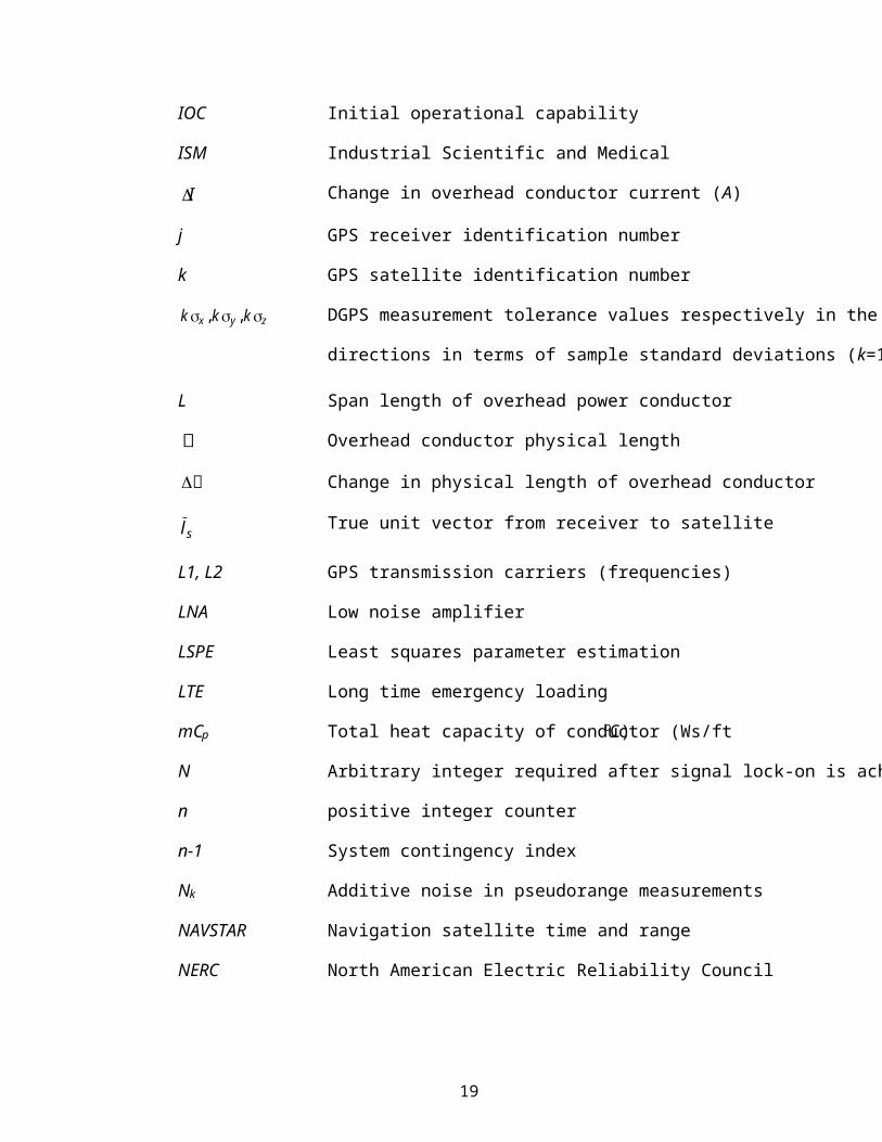
IOC Initial operational capability
ISM Industrial Scientific and Medical
I Change in overhead conductor current (A)
j GPS receiver identification number
k GPS satellite identification number
zyx kkk ,,
DGPS measurement tolerance values respectively in the x, y and z
directions in terms of sample standard deviations (k=1, 2, 3, ...)
L Span length of overhead power conductor
Overhead conductor physical length
Change in physical length of overhead conductor
sl True unit vector from receiver to satellite
L1, L2 GPS transmission carriers (frequencies)
LNA Low noise amplifier
LSPE Least squares parameter estimation
LTE Long time emergency loading
mCp Total heat capacity of conductor (Ws/ft oC)
N Arbitrary integer required after signal lock-on is achieved
n positive integer counter
n-1 System contingency index
Nk Additive noise in pseudorange measurements
NAVSTAR Navigation satellite time and range
NERC North American Electric Reliability Council
20
Accounts for the receiver noise, multipath, inter channel error
(varies with each satellite)
OASIS Open access same time information system
OEM Original equipment manufacturer
p Set of previous readings used to estimate z for the ANNE technique
Pi Change in megawatt generation at bus i
P-code Precise code
PECO Philadelphia Electric Company
PMU Phasor measurement unit
PPS Precise positioning service
pps Pulse per second
PRC Pseudorandom code
PSERC Power Systems Engineering Research Center
PTDF Power transfer distribution factor
Wavelet function
qc
qr
qs
Convected heat loss (watts per lineal foot of conductor)
Radiated heat loss (watts per lineal foot of conductor)
Heat gain from the sun (watts per lineal foot of conductor)
R Resistance
r Exact distance traveled by a given GPS carrier signal
)(13 Rtr Range from satellite 1 to receiver 3 traveled in time, tR
)(14 Rtr Range from satellite 1 to receiver 4 traveled in time, tR
)(23 Rtr Range from satellite 2 to receiver 3 traveled in time, tR
21
)(24 Rtr Range from satellite 2 to receiver 4 traveled in time, tR
ra Range to GPS receiver a
rb Range to GPS receiver b
rr and sr Vectors denoting the true receiver and satellite position respectively
R Denotes the satellite position error
Rk Noiseless pseudorange to the kth satellite
R(Tc) 60Hz resistance per lineal foot of conductor at Tc (/ft)
RTCM SC 104 Radio technical commission for maritime-Special committee 104
Pseudorange
S Transmission time error due to SA
Sc Present overhead power conductor sag
Sp Apparent power
Si Unenergized conductor sag
Sc Change in overhead conductor sag
SA Selective availability
SPS Standard positioning system
SRP Salt River Project
SSTR Steady state thermal rating
STE Short time emergency (STE) loading
STR Static thermal rating
Sample standard deviation
T Moving window width
t time (s)
22
t Differential GPS time corrections
Tc Computed conductor temperature (oC).
eT True tropospheric delay
TI Temperature of an unenergized power conductor
Tm Maximum allowable conductor temperature
T0 Actual ambient air temperature
TR Conductor limit due to conductor thermal capacity
tR Signal reception time at a GPS receiver
TCXO Temperature-controlled crystal oscillator
TSM Temperature-sag model
tT,S Signal transmission time from a GPS satellite
Least squares state estimation parameters
UsiTM Underground Systems Inc.
UTC Universal co-ordinated time
VCO Voltage controlled oscillator
w Overhead conductor weight per unit length
WGS-84 World Geodetic System-1984
WM Weather model
X-Y Cartesian plane
X Correct (true) receiver position
XX Incorrect receiver position
x Abscissa of a Cartesian coordinate
x Statistical mean
23
x Estimated position based on number of satellites in view
x Positioning error (m)
x(k), y(k), z(k) measured set of data chosen to guarantee proper rejection rate in
the x, y, and z directions respectively
x(n), y(n), z(n) n-sampled readings in x, y and z directions that produce vertical
estimation
xk, yk, zk Set of data used to select parameters of the LSPE and ANN
estimators
Xsk, Ysk, Zsk Coordinates of the kth GPS satellite
Xrj, Yrj, Zrj Unknown coordinates of the jth GPS receiver
XTAL Crystal
Y Encrypted P code
y Ordinate in Cartesian coordinate
z Altitude above ellipsoid
Zbus, ni and Zbus, mi Entries in the Zbus matrix referenced to the swing bus
zl Line impedance, rl +jxl of line l
)(ˆ nz Vertical estimation based on n number of readings
z(t) Altitude above ellipsoid (z) measurement at time (t)
z0 Initially known set of altitude above ellipsoid data
1
CHAPTER 1
INTRODUCTION
1.1 Background and Motivation
The electric power industry is undergoing multiple changes and restructuring
towards its deregulation. In this open market environment, transmission services should
be opened to any generation company. This has facilitated the possibility of power sales
far from usual points of electric service. In this context, it is often necessary to monitor
the power handling capability (or available capacity) of the respective transmission
networks in order to serve specific point(s) of the system without compromising the entire
system security. As a motivation to implement this objective of transmission capacity
sales, the OASIS (Open Access Same Time Information System) has been developed [39].
This is an Internet based exchange of information designed to create market for the sale of
available transmission capacity (ATC). Therefore, to be able to rapidly and accurately
determine the capacity of a path has obvious pecuniary value in OASIS.
Overhead conductors form the backbone of power transmission systems.
Electric utilities are under pressure to make optimum use of their existing facilities. In this
respect the overhead high voltage (HV) transmission system is usually a principal
component. In any interconnected HV transmission system, there is the need to define in
quantitative terms the maximum amount of power that may be transferred without violating
the system safety, reliability and security criteria that are in place. Hence, real time ratings
of circuits are critical to system capacity utilization. The current carrying capability of
many transmission circuits is limited by the conductor temperature (thermal limits) and
2
sag. For this reason, real time conductor sag measurement and real time current rating hold
promise for the improvement of system transfer capability.
Traditionally, overhead conductor sag has been considered for line rating by
using indirect measurements. Recent commercialized techniques include the physical
measurement of conductor surface temperature using an instrument mounted directly on
the line, and the measurement of conductor tension at the insulator supports. These
measured parameters can be used to estimate conductor sag. The pertinence of conductor
sag to circuit operation relates to the calculation of dynamic thermal line rating (DTLR).
This takes into account the ambient conditions and/or present operating regime of the
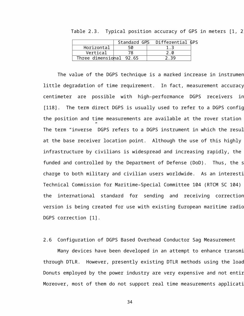
system [13, 15, 18, 20, 21]. DTLR is succinctly defined in Table 1.2.
Most overhead conductors have current ratings based on ground clearance at the
maximum allowable conductor temperature [14, 80, 62]. Ground clearance is a function
of terrain, conductor support geometry and sag. The overhead conductor sag directly
relates to the temperature of the conductor. Therefore, for a given conductor sag
measurement, it is possible to indirectly determine the available extra capacity on a specific
line [15, 64]. This also gives an indication of the possible increase in load without
exceeding the mandated minimum clearance above ground, especially during
contingencies. Thus, real time measurement of conductor sag provides a direct
measurement of the primary limiting parameter (i.e., mandated clearance).
On the basis of this concept, a new direct method for the measurement of
overhead conductor sag using differential global positioning satellite (DGPS) system has
been proposed for the purpose of DTLR. This sag monitoring device responds to the
weather conditions along an entire line section rather than at a single point along the line.
The main advantages of the method include the accurate measurement of conductor sag
3
without recourse to simplified assumptions that could otherwise affect its accuracy. With
this method, errors caused by insulator swings could be eliminated [62]. To be able to
directly monitor and display the conductor sag or clearance in real time will enable
prospective engineers to physically capture the conductor behavior, and to take judicious
steps towards a reliable system loading.
The North American Electric Reliability Council (NERC) defines security as the
“prevention of cascading outages when the bulk power supply is subjected to severe sudden
disturbances” [122]. Security limits relating to key power system parameters are therefore
established and the power system is operated within these limits. This is done in order to
withstand the occurrence of certain disturbances in the bulk power supply. Thus, meeting
specific constraints pertinent to system loading and stability conditions, permissible
operating bus voltage magnitudes, generator angle limits, and the restoration to acceptable
steady state conditions following a transient. Some of these instability limits are dynamic
in nature (e.g., voltages, angles, etc.). Therefore, dynamic security analyses are conducted
to ascertain that operating constraints/limits are not violated, and also to insure that a
transient will result in an acceptable operating condition. Also of interest in the dynamic
case is the transition itself. For dynamic security analysis, contingencies are not considered
only in terms of post contingency conditions (i.e., outages) but also in terms of the total
disturbance.
At this point, it is illuminating to discuss the way line limits of diverse types vary
with line length. This discussion is semi-technical and informal because a full treatment
of the subject would take too much space, and would divert attention from the main subject
of the dissertation. Consider two types of overhead transmission line limits:
Type “TR” due mainly to the thermal capacity of the conductors
4
Type “D R” due mainly to the evolution of the system operating state (dynamic
state response) with time.
Type TR is strictly a function of the physics of overhead transmission conductors and their
thermal characteristics. Type TR is physically independent of line length. Type DR , on the
other hand, relates to the passage of power over a line length in an AC power system.
This power flow involves system dynamic response. Type DR limits are closely dependent
on transmission line length, and therefore line reactance. It is more difficult to transport
power over a long distance compared to a short distance. Therefore, one expects that type
TR limits are approximately constant with respect to line length. However, type D R limits
decrease with increasing transmission line length. This implies that the line length
crossover of TR with DR determines a line length below which TR is the limiting factor and
above which the DR is critical.
1.2 Objectives and Scope
This dissertation work relates to overhead conductor sag instrumentation, study and
use of measurements from the DGPS system to determine the real time sag in HV overhead
power transmission lines. The system is intended to provide accurate overhead HV
conductor sag measurement at a modest cost. The primary objectives consist of the
following:
Development, design, construction and performance of selected tests on an
instrument based on the DGPS technology to measure, in real time, overhead
HV transmission conductor sag
Design and testing of selected digital signal processing tools applicable to the
practical operation of the overhead conductor DGPS sag instrument
5
The secondary objectives include:
Outlining the instrument limitations and ways to overcome these limitations in a
commercialized instrument
Modeling noise in DGPS vertical measurements
Framework proposal about a methodology on how real time overhead conductor
sag measurements may be used for DTLR
The code mandated conductor clearance above ground is the key limiting factor in
this method. This new approach is expected to provide a competitive alternate tool for real
time monitoring of overhead conductor sag. Based on the conductor sag information, the
resulting DTLR could be used in conjunction with known operating points to determine
the ATC of overhead power transmission networks. This may then be readily accessible
to every electricity market participant (e.g. power exchange and scheduling coordinators)
in the transmission network.
Note that the network dynamic security limits relate to the operating state and the
system dynamic response rather than conductor ground clearance. The issue of dynamic
security limits is not discussed in this work. The main focus is on overhead conductor
thermal ratings.
1.3 GPS Technology and Power Systems
The Global Positioning Satellite (GPS) system is a state-of-the-art timing and
positioning system based on 24 satellites, launched and maintained by the United States
government. This system of satellites, launched for the first time in 1973 reached its initial
operational capability (IOC) in 1993 with 24 satellites, and became fully operational in
1994. Presently, the GPS consists mainly of a segment of 24 satellites placed
6
asymmetrically in six orbital planes with an orbital plane inclination of 55 degrees relative
to the equatorial plane, a ground control segment and user receivers [1, 2, 3, 30, 43, 45].
Due to the progressive developments in the satellite-based navigation and time transfer
system, the GPS is continuously providing unprecedented levels of accuracy, leading to
both extensive military and civilian use. Its main applications have been in the areas of
navigation, surveying, aircraft navigation and landing systems, farming, weather
forecasting, fleet management and military applications. The following accounts for the
increase use of DGPS: nanosecond-order precise time tagging capability, compactness,
portability, low cost, and round the clock operation in all weather conditions anywhere on
Earth. DGPS has been used for different applications including dispatching/fleet
management and emergency tracking [19, 71, 78, 79]. Now, in a mature state, the GPS has
spawned applications that go beyond the usual positioning of aircraft and ships. The ability
of the GPS technology to provide time synchronization in the order of nanoseconds over a
wide area has opened up new possibilities for a secure and reliable operation of electric
power systems [31, 32, 33, 34, 35, 36, 37]. Table 1.1 depicts some selected GPS
applications.
7
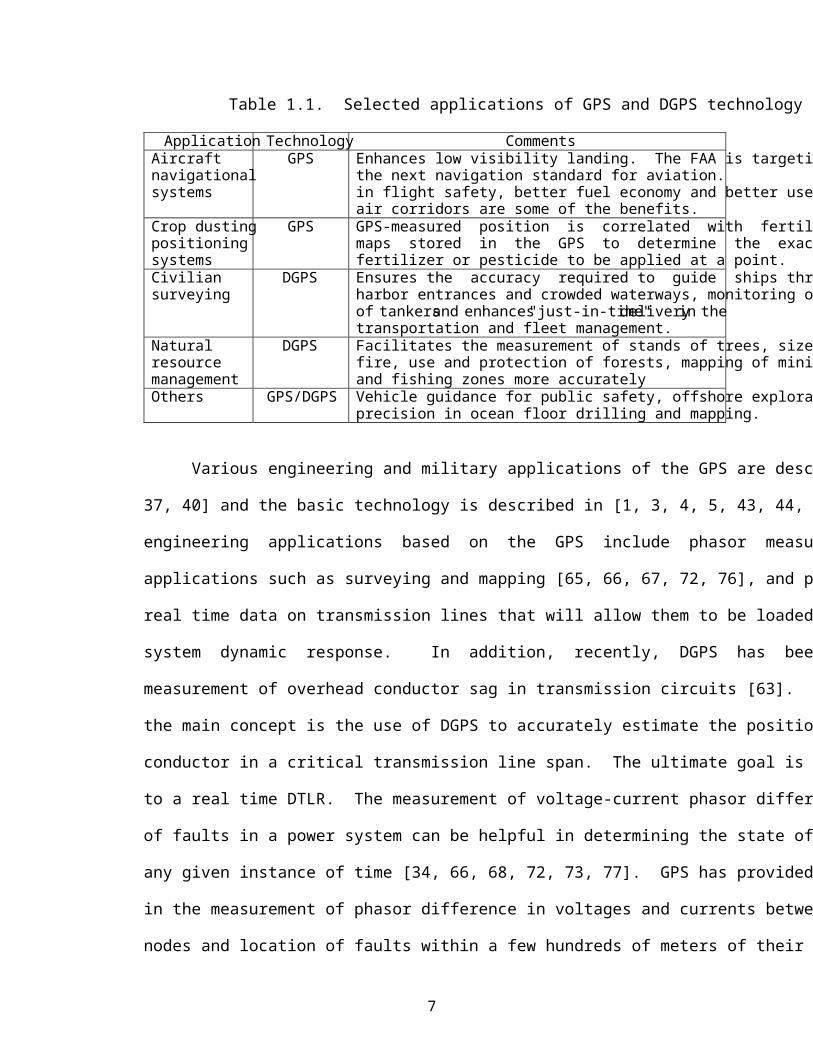
Table 1.1. Selected applications of GPS and DGPS technology
Application Technology Comments Aircraft navigational systems
GPS Enhances low visibility landing. The FAA is targeting GPS as the next navigation standard for aviation. Improvement in flight safety, better fuel economy and better use of crowded air corridors are some of the benefits.
Crop dusting positioning systems
GPS GPS-measured position is correlated with fertilizer demand maps stored in the GPS to determine the exact amount of fertilizer or pesticide to be applied at a point.
Civilian surveying
DGPS Ensures the accuracy required to guide ships through tricky harbor entrances and crowded waterways, monitoring of fleets of tankers and enhances "just-in-time" delivery in the transportation and fleet management.
Natural resource management
DGPS Facilitates the measurement of stands of trees, size of forest fire, use and protection of forests, mapping of mining tracts, and fishing zones more accurately
Others GPS/DGPS Vehicle guidance for public safety, offshore exploration and precision in ocean floor drilling and mapping.
Various engineering and military applications of the GPS are described in [35, 36,
37, 40] and the basic technology is described in [1, 3, 4, 5, 43, 44, 45, 47]. The main power
engineering applications based on the GPS include phasor measurement, positioning
applications such as surveying and mapping [65, 66, 67, 72, 76], and potentially in deriving
real time data on transmission lines that will allow them to be loaded to a limit relating to
system dynamic response. In addition, recently, DGPS has been proposed for the
measurement of overhead conductor sag in transmission circuits [63]. In that application,
the main concept is the use of DGPS to accurately estimate the position of a point on the
conductor in a critical transmission line span. The ultimate goal is to convert this sag data
to a real time DTLR. The measurement of voltage-current phasor difference and location
of faults in a power system can be helpful in determining the state of the power system at
any given instance of time [34, 66, 68, 72, 73, 77]. GPS has provided a unique opportunity
in the measurement of phasor difference in voltages and currents between widely dispersed
nodes and location of faults within a few hundreds of meters of their origin. This process
8
which could otherwise require considerable post-fault location efforts is easily achievable
by using GPS time reference.
Precise time-tagged fault data has proved invaluable for post-fault analysis [34, 35,
67, 68]. This ultimately leads to improved efficiency and greater reliability in power
system operation. The GPS time reference is also known to be used to synchronize the
measurement of system voltages and currents which allow network-wide measurement of
busbar phase angles [33, 40]. Locating power line faults and real time phasor
measurements require very precise timing. GPS has proved very successful in this respect.
The use of synchronized phasor measurement units (PMUs) are usually time critical. These
make use of precise timing signals derived from GPS to time-tag measurements of
alternating current signals. The Bonneville Power Administration (BPA) has used the
precise timing feature of the GPS to enhance power system performance and reliability
since 1988. For example both the Traveling Wave Locator and the PMUs of BPA possess
built-in GPS receiver that provide accurate timing to reduce the time and cost associated
with repairing faulty lines, minimize consequential losses and degraded reliability incurred
during contingencies [34, 37]. GPS synchronized phasor measurement equipment has been
known to record the dynamic response of power system phase angles during short circuits
[36]. GPS is now being used extensively by the telecommunication industry [32]. With
the advancing technology and reduced cost, GPS holds considerable applications in the
future. A summary of some suggested future GPS applications in the power engineering
area is given in [72].
9
1.4 Preambles of Conductor Capacity Ratings
Transmission lines across the country are recently being operated at higher
temperatures [64, 80, 107, 117]. Two key factors driving the changes in the way utilities
operate their transmission systems can be attributed to the increased population growth,
and the necessity to maximize equitable return on investment in the electricity deregulation
era. Population growth per se has not only increased power demand, but also reduced the
available rights-of-way for new transmission lines. For the purpose of curtailing
investments, a probable option for increasing power transfer capability is to operate lines
at significantly higher loading levels than ever before. However, increasing line currents
results in higher ohmic losses, which in turn, together with ambient conditions, influence
conductor temperatures with an associated increase in conductor sag due to material
expansion. This leads to reduced conductor clearances to ground. It is very important for
electric power utility companies to know the power level that can be transmitted over their
power transmission lines at any given time. This enables them to serve load reliably and
to secure adequate and equitable financial gains without compromising system-wide
reliability during normal operating conditions, and more particularly during system
contingencies. For this reason, both the conductor thermal and mandated sag limits must
be evaluated.
The conductor sag is a reversible process provided the yield strength of the
conductor material is not exceeded. In a transmission circuit, one or more limiting (critical)
spans are usually identified as the tower-to-tower segments of the circuit which are the
limiting elements in the entire circuit. The sag of the conductor in the limiting span or the
conductor ground clearance is one of the critical parameters in the determination of ATC
of the circuit. In order to preserve conductor life for practical purposes, various conductor
10
load carrying capability levels are imposed to ensure safer conductor thermal limits [15,
56, 64, 81].
The conductor thermal limit relates to conductor temperature and sag, and it is often
a main concern especially for circuits that are heavily loaded. The thermal capacity of
overhead conductors depends on conductor temperature due to ambient air temperature,
ohmic heating, incident solar radiation, local wind speed and wind direction, limiting
For purposes of DTLR, these parameters must be accurately determined since operating
conductors at higher temperatures for longer duration of time could cause irreversible aging
phenomena, referred to as annealing and creep. This could lead to a total loss of conductor
life. The overhead conductor may be loaded conservatively or dynamically.
Typically, worst case weather conditions [14, 18, 56, 59] are assumed in the case
of conservative loading but, actual weather conditions are taken into account for the DTLR
case. In either case, the conductor load must produce a conductor temperature such that
there is no permanent loss of strength by annealing or creep. In many instances however,
it may be possible to load the transmission circuit for a short period of time beyond the
conventional thermal limit of the overhead conductor, provided the conductor ground
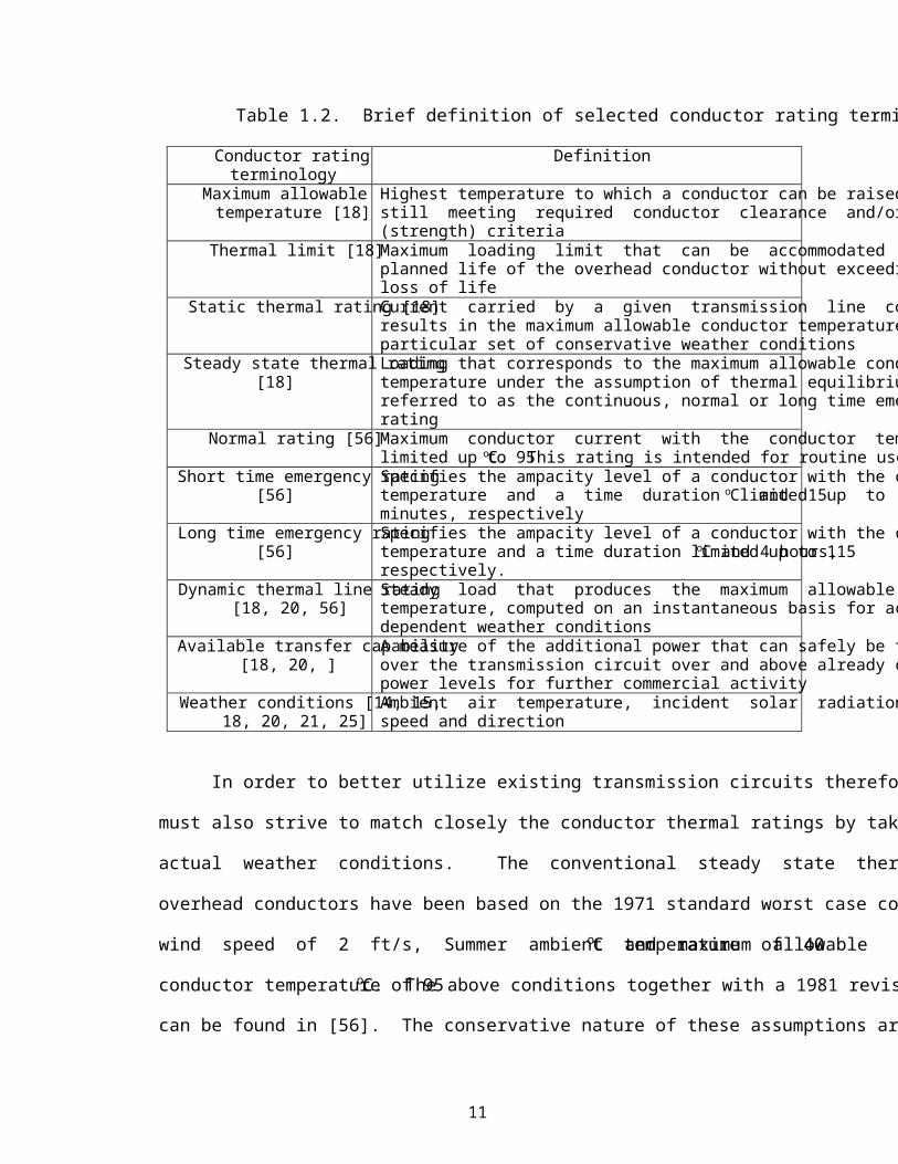
clearance is constrained to a specified mandated limit. Table 1.2 gives a brief description
of some selected terminology commonly used to describe overhead conductor ratings.
Some of these concepts are also described in detail in references [13, 14, 15, 16, 17, 18,
20, 21, 24, 26, 56, 58, 62, 64].
11
Table 1.2. Brief definition of selected conductor rating terminology
Conductor rating terminology
Definition
Maximum allowable temperature [18]
Highest temperature to which a conductor can be raised while still meeting required conductor clearance and/or loss of life (strength) criteria
Thermal limit [18] Maximum loading limit that can be accommodated over the planned life of the overhead conductor without exceeding 100% loss of life
Static thermal rating [18] Current carried by a given transmission line conductor which results in the maximum allowable conductor temperature for a particular set of conservative weather conditions
Steady state thermal rating [18]
Loading that corresponds to the maximum allowable conductor temperature under the assumption of thermal equilibrium. Also, referred to as the continuous, normal or long time emergency rating
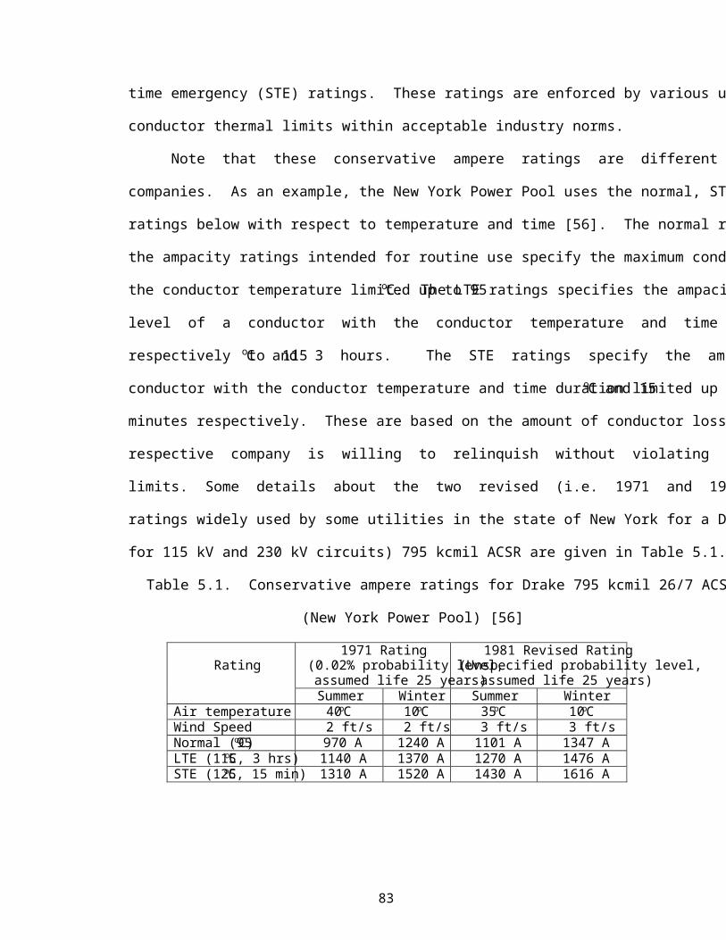
Normal rating [56] Maximum conductor current with the conductor temperature limited up to 95oC. This rating is intended for routine use
Short time emergency rating [56]
Specifies the ampacity level of a conductor with the conductor temperature and a time duration limited up to 125oC and 15 minutes, respectively
Long time emergency rating [56]
Specifies the ampacity level of a conductor with the conductor temperature and a time duration limited up to 115oC and 4 hours, respectively.
Dynamic thermal line rating [18, 20, 56]
Steady load that produces the maximum allowable conductor temperature, computed on an instantaneous basis for actual time dependent weather conditions
Available transfer capability [18, 20, ]
A measure of the additional power that can safely be transferred over the transmission circuit over and above already committed power levels for further commercial activity
Weather conditions [14, 15, 18, 20, 21, 25]
Ambient air temperature, incident solar radiation, local wind speed and direction
In order to better utilize existing transmission circuits therefore, utility companies
must also strive to match closely the conductor thermal ratings by taking into consideration
actual weather conditions. The conventional steady state thermal ratings of certain
overhead conductors have been based on the 1971 standard worst case conditions such as
wind speed of 2 ft/s, Summer ambient temperature of 40oC and maximum allowable
conductor temperature of 95oC. The above conditions together with a 1981 revised version
can be found in [56]. The conservative nature of these assumptions are due to the lack of
12
actual knowledge of the conductor operating conditions. The utilization of the extra
capacity of the system by operating conductors at higher load levels in real time could
serve as an option for an improvement in power wheeling. This is a potential source of
reduction in capital and operating costs [16, 21, 23, 58, 64, 80].
1.5 Dynamic Thermal Line Ratings
Deregulation has opened the doors of power industries to a more competitive
electricity market. This raises the level of interest on the thermal capability of overhead
conductors for the maximum power transfer capacity from one point of a transmission
circuit to another. The recognition of the limitations of the conservative steady state ratings
and the potential benefits of a DTLR system has been an interesting issue in recent years.
Real time thermal rating methods have been given various names including DTLR [15, 16,
17, 18, 21, 23, 24, 56, 57, 58, 64].
DTLR is a method described by the process of favorably adjusting the thermal
ratings of power equipment for actual weather conditions and load patterns. This is the
case, particularly if an overload which causes a small conductor loss of life or strength but
never violates the code mandated clearance is to be applied for an acceptable period of
time. There appears to be no firm industry standard for DTLR methods. In many areas
of the world, it is increasingly difficult to build additional power transmission lines.
Erecting new lines or physically upgrading older transmission facilities can require high
costs and lengthy public hearings. DTLR systems can generally provide a relatively low
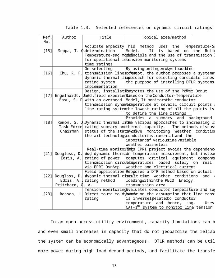
cost alternative to a new infrastructure. A summary of selected references on dynamic
ratings are shown in Table 1.3.
13
Table 1.3. Selected references on dynamic circuit ratings
Ref. No.
Author Title Topical area/method
[15]
Seppa, T. O.
Accurate ampacity determination: Temperature-sag model for operational real time ratings
This method uses the Temperature-Sag Model. It is based on the Ruling Span principle and the use of transmission line tension monitoring systems
[16]
Chu, R. F.
On selecting transmission lines for dynamic thermal line rating system implementation
By using contingently overloaded line concept, the author proposes a systematic approach for selecting candidate lines for the purpose of installing DTLR systems
[17]
Engelhardt, J.S.,
Basu, S. P.
Design, installation, and field experience with an overhead transmission dynamic line rating system
Promotes the use of the Power Donut TM. Based on the Conductor-Temperature Model, It monitors the conductor temperature at several circuit points and the lowest rating of all the points is used to define the line ratings
[18]
Ramon, G. J. Task Force Chairman
Dynamic thermal line rating summary and status of the state-of-the-art technology
Provides a summary and background of the various approaches to increasing line thermal capacity. The methods discussed involve monitoring weather conditions, conductor instrumentation and the importance of various time variable weather parameters
[21]
Douglass, D. A.,
Edris, A.
Real-time monitoring and dynamic thermal rating of power transmission circuits via EPRI DynAmp
This EPRI project avoids the dependence on temperature measurement, but instead computes critical equipment component temperatures based solely on real time weather and electrical current
[22]
Douglass, D. A.,
Edris, A., Pritchard, G. A.
Field application of a dynamic thermal circuit rating method
Proposes a DTR method based on actual real time weather conditions and circuit loading within the PECO Energy transmission area
[23]
Reason, J.
Tension monitoring: Direct route to dynamic rating
Evaluates conductor temperature and sag based on the assumption that line tension is inversely related to conductor temperature and hence, sag. Uses the CAT-1TM system to monitor line tension
In an open-access utility environment, capacity limitations can be very expensive,
and even small increases in capacity that do not jeopardize the reliability and security of
the system can be economically advantageous. DTLR methods can be utilized to deliver
more power during high load demand periods, and facilitate the transfer of power with
14
relatively little extra equipment investment. A literature survey and actual utility data
reveal that dynamic thermal ratings of overhead conductors usually exceed steady state
ratings 70-80 percent of the time for certain defined periods of the day [21, 26, 38]. A
speculated increase in transmission capabilities by 15-30% exists for tension monitoring
systems that are intended for DTLR purposes [121].
1.6 Contemporary Dynamic Thermal Rating Models
The inherent conservatism in existing conductor rating methods often results in the
transmission circuit being underutilized. In recent years, many authors including [15, 16,
17, 18, 21, 22, 23, 24, 26] and EPRI have intensified research and proposal of various
DTLR methods as a strategic option for transmission system operators. There has also
been a considerable interest in the topic by some major utility related companies including
the Usi/Nitech, General Electric Company, Niagara Mohawk Power Corporation, Detroit
Edison, Valley Group in Ridgefield, Connecticut, Power Technologies Inc., of
Schenectady, New York, the Electric Power Research Institute (EPRI), Palo Alto,
California, and LineSoft of Spokane, Washington. Most of the proposed methods measure
some related parameters, which are then used to indirectly compute the overhead conductor
sag. Of those indirect methods for determining conductor sag, the most common procedure
employs tension measurements and ruling span assumptions [15, 23, 80]. The main
achievements so far have been to describe the pertinence of the method, concept and its
benefits to the power industry especially in this era of competitive electricity markets.
Among the dynamic rating system equipment providers for overhead conductors
are The Valley Group Inc. and the USiTM, Inc. The "CAT-1" transmission line rating
system [121] of the Valley Group, Inc., incorporates the use of load cells to monitor the
15
mechanical tension of both ruling span sections and deadend structure for overhead
transmission conductors. This is then used to modify the operational ampacity of the
conductor [14, 15]. Based on tension monitoring, DTLR systems of EPRI have been
installed in utilities such as BC Hydro, PECO Energy, and Illinois Power Company. The
CAT-1 system does not measure conductor sag directly. The CAT-1 instrument is
designed for temporary initiation of tension measurements at a preset time interval (ten
minutes usually). Therefore it may not be suitable for real time applications. The
USiTM/Nitech proposes the use of a combined Power Donut TM sensor and ground weather
station systems integrated with a dynamic rating software (UPRATE TM) and hardware to
provide a DTLR system based on load, conductor temperature, ambient temperature and
wind measurements. For example, the Plus-1 Power Donut system is designed for
temporary monitoring of line-to-ground voltage, phase current, power factor and
(optionally) power line surface temperature on electrical transmission and distribution lines
without the need to interrupt electrical service. It can be used for capacitor placement
studies, planning surveys, temporary and emergency metering, and to some extent for
DTLR studies. The main disadvantage of the Power Donut system is that of economics.
It requires installation of several ground weather stations and Power Donuts on the
conductor. The application of the Power Donut for DTLR purposes may be possible but it
is not designed for real time applications. Although the existing DTLR systems have not
been thoroughly assessed, there seems to exist a potential source of weakness in terms of
measurement precision and cost since they do not measure the overhead conductor sag
directly. The DGPS based sag instrument is likely to require installation of fewer units for
a given transmission network compared to existing systems.
16
In summary, three traditional methods can be identified in industry practices for
DTLR based on the measured parameters [13, 15, 18, 21, 22, 23, 81]. These are the: (1)
weather-based models, (2) conductor temperature-based model, and (3) the conductor
tension-based model. Other proposed DTLR methods are based on the Ruling Span
principle [15, 27, 80] and the use of transmission line tension monitoring systems. This is
known by the name “Temperature-Sag Model” (TSM) [15]. The accuracy of these models
depends on the accurate determination of the conductor temperature which is also a
function of ambient air temperature, solar radiation, wind speed and direction.
The resulting inaccuracies in the weather-based model emanate from the error
sources in the weather/conductor temperature calculations, the weather observations, the
spatial variability of wind as well as the error sources caused by unknown line design
factors. The conductor temperature can be measured by the aid of temperature sensors.
The accuracy of the temperature measurement itself becomes questionable or deteriorates
when the heat sink effect is taken into account [14, 15, 64]. The errors in the tension-based
model originate from the inaccuracy in the tension measurement itself and the intermediate
average conductor temperature computations. A similar model based on real time
conductor sag monitoring is possible but no such commercial device presently exists [64].
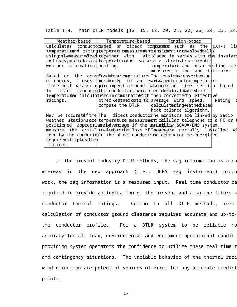
The main DTLR methods that are in operation presently are described in Table 1.4. Each
type of model has its own advantages and disadvantages in a particular application.
Weather-based Temperature-based Tension-based Calculates conductor temperature and ratings using only measured load and uses public domain weather information.
Based on direct conductor temperature measurement together with air temperature and solar heating.
Systems such as the CAT-1 line tension monitor uses load cells placed in series with the insulators at a strain structure. Air temperature and solar heating are measured at the same structure.
Based on the conservation of energy, it uses the steady state heat balance equations to track conductor temperature and calculate ratings.
Conductor temperature is converted to an equivalent wind speed perpendicular to the conductor, which is then used in combination with other weather data to compute the DTLR.
The tension is converted to an average conductor temperature along the line section based on field calibration data, which is then converted to effective average wind speed. Rating is calculated using weather based heat balance algorithm.
May be accurate if the weather stations are positioned appropriately to measure the actual weather seen by the conductor. Requires multiple weather stations.
The direct conductor temperature measurement is an advantage if the rating is to limit the loss of strength in the phase conductors.
The monitors are linked by radio or cellular telephone to a PC or to a utility SCADA/EMS system. They are normally installed with the conductor de-energized.
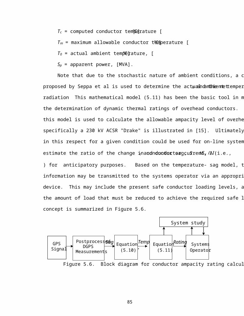
In the present industry DTLR methods, the sag information is a calculated output,
whereas in the new approach (i.e., DGPS sag instrument) proposed in this dissertation
work, the sag information is a measured input. Real time conductor rating systems are
required to provide an indication of the present and also the future status of the overhead
conductor thermal ratings. Common to all DTLR methods, remains the fact that the
calculation of conductor ground clearance requires accurate and up-to-date information on
the conductor profile. For a DTLR system to be reliable however, it must guarantee
accuracy for all load, environmental and equipment operational conditions in addition to
providing system operators the confidence to utilize these real time ratings under all normal
and contingency situations. The variable behavior of the thermal radiation, wind speed and
wind direction are potential sources of error for any accurate prediction of future operating
points.
18
1.7 Organization
This dissertation work deals with the proposal of the design, construction and
testing of a DGPS based instrument for the measurement of overhead HV conductor sag.
A brief introduction to the motivation of this work in general, GPS/DGPS and its
applications in power engineering and other areas, as well as overhead conductor rating
methodologies are described in Chapter 1. Chapter 2 presents a detailed background to the
GPS/DGPS technology. The main concept and components of the proposed instrument,
its basic configuration, results of experimental tests and preliminary conclusions are given
in Chapter 3. Chapter 4 presents field trial measurements, and data analysis using various
DSP methodology to improve the DGPS based conductor sag instrument measurement
accuracy. The DSP techniques used are bad data identification and modification, least
squares parameter estimation (LSPE), artificial neural network estimation (ANNE) and the
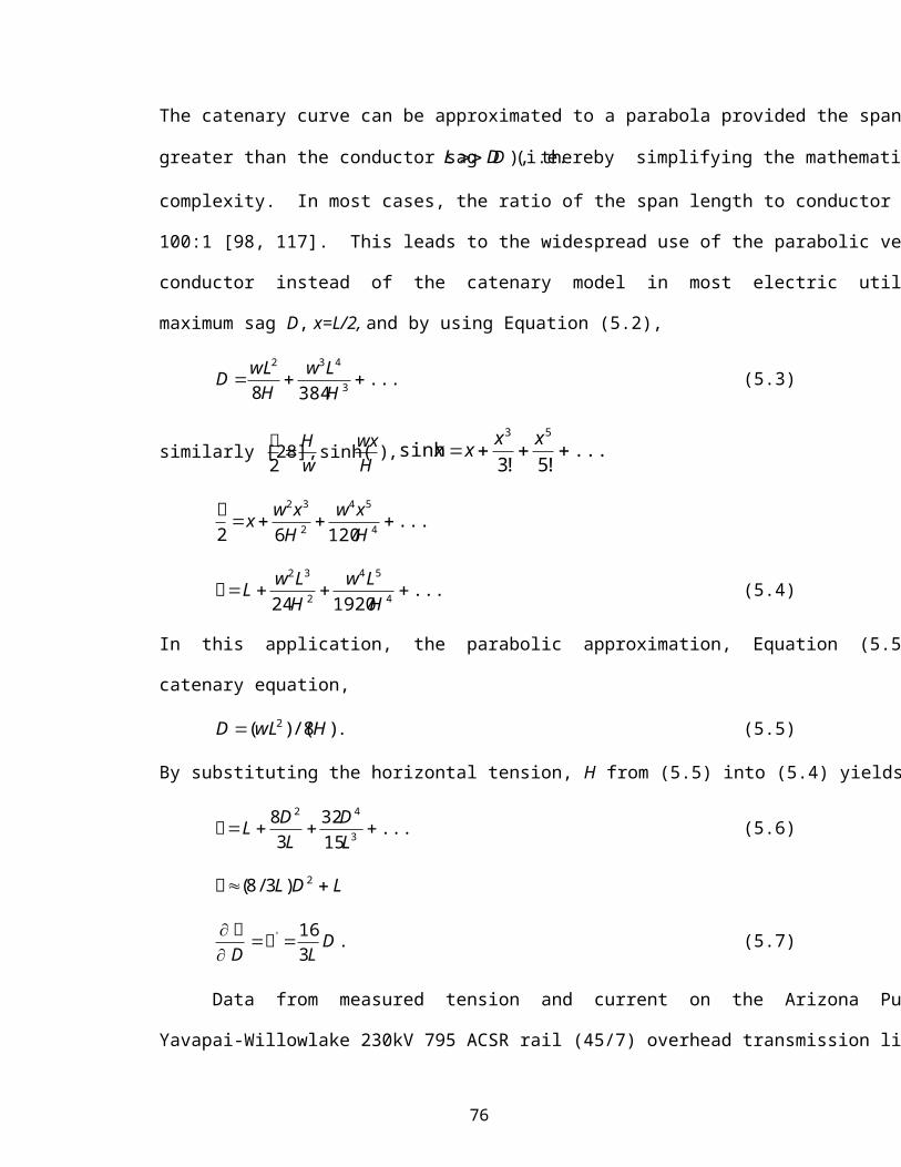
Haar wavelet transforms. A brief mathematical model of overhead HV conductors, main
factors affecting conductor ratings and a proposed outline for the integration of the
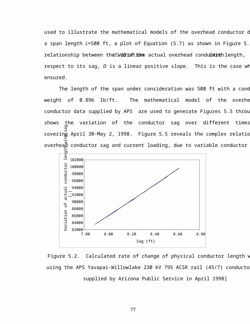
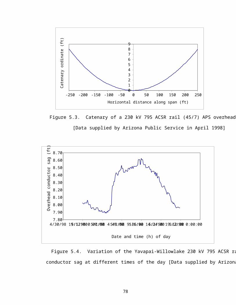
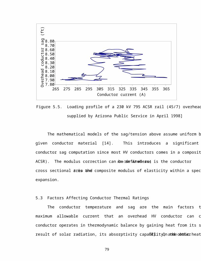
overhead conductor sag information for DTLR purposes are described in Chapter 5. Some
concluding remarks and recommendations for future work are contained in Chapter 6. The
appendices show illustrative photographs of the DGPS and radio modem receiver units,
various measured data based on the proposed DGPS conductor sag instrument and
MATLAB source codes together with brief explanations for the implementation of the DSP
methods used.
19
CHAPTER 2
THE GLOBAL POSITIONING SATELLITE SYSTEM
2.1 Brief Description
It might be said that the Global Positioning Satellite (GPS) system is to location as
the digital clock is to time. The GPS and its Russian counterpart, Global Orbiting
Navigation Satellite System (GLONASS) transmits signals every second which upon
decoding, allow the date and time of the day to be determined to a nanosecond accuracy
anywhere in the World. The Navigation Satellite Timing and Ranging (NAVSTAR) GPS
was developed, launched and maintained by the United States government as a worldwide
navigation and positioning resource for both military (i.e. precise positioning service
(PPS)) and civilian (i.e. standard positioning service (SPS)) applications. It is based on a
constellation of 24 satellites in 55o [1, 2, 3, 11] inclined orbits to the equatorial plane. The
system transmits extremely precise timing signals that allow a GPS receiver anywhere on
Earth to be used for a variety of purposes, and in particular to determine position. Each
satellite orbits the Earth once every 12 hours, repeating the same trajectory and
configuration each time [1, 2, 3, 4, 30, 43, 44, 45]. According to Trimble Navigation
Limited [1, 2], the orbital motion of each satellite is constantly monitored by five ground
monitoring stations at Hawaii, Ascension Island, Diego Garcia, Kwajalein, and Colorado
Springs so that their instantaneous positions are known with great precision. The master
ground station transmits corrections for the satellite ephemeris constants and clock offsets
back to the satellites themselves. The satellites can then incorporate these updates in the
signals they send to GPS receivers. The method relies on accurate time-pulsed radio
signals in the order of nanoseconds from high altitude Earth orbiting satellites of about
20
11,000 nautical miles, with the satellites acting as precise reference points. These signals
are transmitted on two carrier frequencies known as L1 and L2.
2.2 Mode of Operation
The GPS system determines location measurements by timing the time it takes the
radio signal, traveling at the speed of light c (i.e. 3x10 8 m/s) from a GPS satellite to reach
a receiver. Each GPS satellite transmits two radio signals: a carrier and a unique
pseudorandom code (PRC). This code allows the GPS system to work with very low-
power signals and small antennae. It provides a means to unambiguously match signals of
a satellite and receiver for timing purposes and to control access to satellites by changing
the code in times of war. The GPS is designed such that each satellite has its own distinct
PRC code thereby making comparison very easy at the respective receiver locations. The
signals are timed by an atomic clock in the satellite, and the GPS receiver generates a
matching code timed by its own synchronized clock. This calculation is generally
performed using the PRC signal, but the carrier signal can be used instead for better
precision.
In order to achieve a signal reception, a GPS receiver has to extract two separate
information which are encoded into the transmitted message. The first is a 1 pps strobe
pulse produced every second and the other is a serial message which contains the date and
time of the previous 1 pps strobe based on the Universal Co-ordinated Time (UTC)
standard. An ASIC (application-specific integrated circuit) then selects the stronger
signals, allows for the propagation delays between satellites and the receiver, and outputs
the 1 pps signal (synchronous to 1 ns) and the UTC message. For each of the several
satellites, the user equipment measures a pseudorange and modulates the navigation
21
message. A pseudorange in GPS application can be defined as the true range (i.e. distance)
in addition to an unknown bias which is equal to the product of the speed of light and the
difference between the receiver clock and the GPS satellite time. Pseudorange
measurements to four well-spaced satellites are sufficient to determine the three
dimensional position and clock offset of the user. When signals from at least three satellites
are received, the receivers position can be determined with a precise accuracy depending
on the receiver engine. Over four satellites are usually available in GPS measurements, all
of which are used to obtain a least square fit of the four unknown parameters (x, y, z and t).
The first three satellites are used to triangulate a position. The fourth is used to improve
the position accuracy by accounting for the time offset between the satellite clock and the
GPS receiver clock which may not necessarily coincide. The fundamental GPS equations
involving positioning are based on the ideal simultaneous iterative least squares solution
as defined in Equation (2.1) with the center of the Earth acting as the initial guess position
[7, 8, 9, 10],
2222 )()()()( dTRZZYYXX krjskrjskrjsk , k = 1, 2,…, n 4 (2.1)
where (Xsk, Ysk, Zsk) and (Xrj Yr, Zrj) represent the positions of the kth satellite and the
unknown jth receiver respectively, Rk denotes the noiseless pseudorange to the k th satellite
and dT is the unknown receiver clock bias converted to distance. The pseudorange is
described in terms of the longitude and latitude measurements of the receiver (i.e.,
effectively x and y), the altitude of the receiver (effectively z), and the time t at which the
measurement was made. However, in practice the pseudorange measurements usually
contain randomly changing errors hence, the problem becomes highly stochastic. An
incorporation of an additive noise Nk in the pseudorange measurements to account for real
situations transforms Equation (2.1) as follows,
22
2222 )()()()( dTNRZZYYXX kkrjskrjskrjsk . (2.2)
A discussion is given for similar equations and their solutions in [7, 8, 9, 10].
Digital signal processing (DSP) techniques can be used to further enhance the accuracy by
a series of position and time measurements to minimize error. Interestingly, the GPS
transmission is made at low power level (the signal strength at the point of reception is
about –90 to –120 dBm). The signal to noise ratio is very low at the surface of the Earth
at this power level. The attenuation of the noise is accomplished by averaging the received
signal: the noise is averaged and a distinctively coded signal appears as an output. The
averaging process as well as the solution of Equation (2.1) is the main time limiting process
that determine how often a GPS measurement can be made. Recent advances in signal
processing permit these weak satellite signals to be received by a small antennae, hence
reducing the size and weight of the overall GPS package.
2.3 Signal Carriers
The GPS signal is basically a time pulse hence, it contains very little information.
The GPS satellites transmit radio signals on two carrier (L1 and L2) frequencies. The use
of two radio frequencies allows for the correction of ionospheric delay errors and the wider
bandwidth allows more accurate ranging thereby further improving the positioning
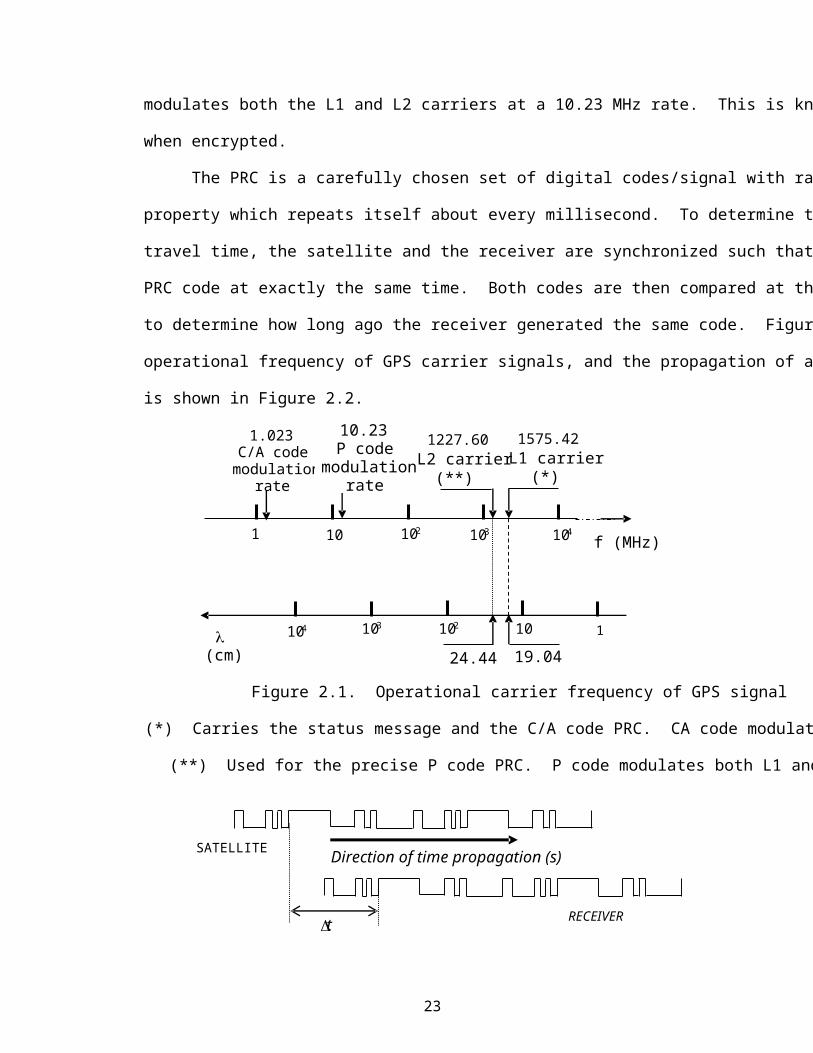
accuracy. The L1 carrier is 1575.42 MHz and carries both the status message and a PRC
for timing. The L2 carrier is 1227.60MHz and is used for the more precise military PRC.
There are two types of PRCs. These are the C/A (coarse acquisition) and P (precise) codes.
The C/A code modulates the L1 carrier. It repeats every 1023 bits and modulates at a 1
MHz rate [43, 44, 45]. The more accurate P code repeats on a seven day cycle and
23
modulates both the L1 and L2 carriers at a 10.23 MHz rate. This is known as the “Y” code
when encrypted.
The PRC is a carefully chosen set of digital codes/signal with random noise-like
property which repeats itself about every millisecond. To determine the satellite signal
travel time, the satellite and the receiver are synchronized such that they generate the same
PRC code at exactly the same time. Both codes are then compared at the receiver location
to determine how long ago the receiver generated the same code. Figure 2.1 illustrates the
operational frequency of GPS carrier signals, and the propagation of a typical PRC signal
is shown in Figure 2.2.
Figure 2.1. Operational carrier frequency of GPS signal
(*) Carries the status message and the C/A code PRC. CA code modulates the L1 carrier
(**) Used for the precise P code PRC. P code modulates both L1 and L2 carriers
t RECEIVER
SATELLITE Direction of time propagation (s)
1575.42 1227.60 L1 carrier
(*) L2 carrier
(**)
1 10 102 103 104
1 104 103 102 10
f (MHz)
(cm) 24.44 19.04
1.023 C/A code
modulation rate
10.23 P code
modulation rate
24
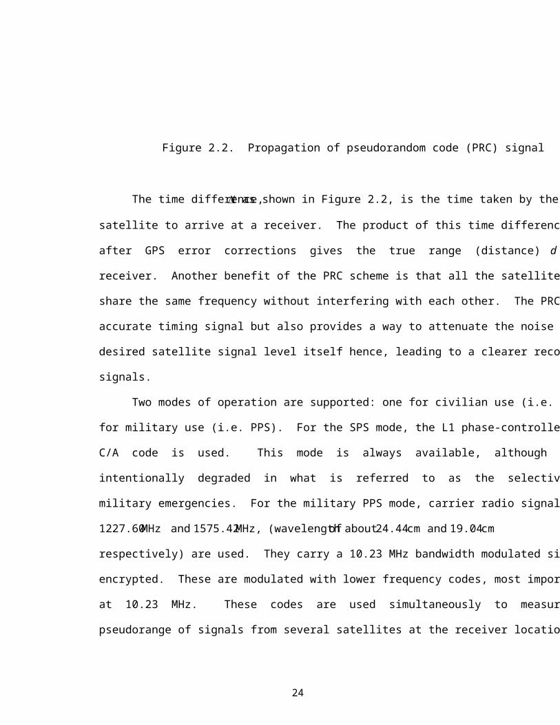
Figure 2.2. Propagation of pseudorandom code (PRC) signal
The time difference, t as shown in Figure 2.2, is the time taken by the PRC of a
satellite to arrive at a receiver. The product of this time difference and the speed of light
after GPS error corrections gives the true range (distance) d between a satellite and a
receiver. Another benefit of the PRC scheme is that all the satellites in the system can
share the same frequency without interfering with each other. The PRC not only acts as an
accurate timing signal but also provides a way to attenuate the noise without reducing the
desired satellite signal level itself hence, leading to a clearer recognition of the faint GPS
signals.
Two modes of operation are supported: one for civilian use (i.e. SPS) and the other
for military use (i.e. PPS). For the SPS mode, the L1 phase-controlled carrier radio signal
C/A code is used. This mode is always available, although its accuracy may be
intentionally degraded in what is referred to as the selective availability (SA) during
military emergencies. For the military PPS mode, carrier radio signal transmissions on
1227.60 MHz and 1575.42 MHz, (wavelength of about 24.44 cm and 19.04 cm
respectively) are used. They carry a 10.23 MHz bandwidth modulated signal that may be
encrypted. These are modulated with lower frequency codes, most importantly the P-code
at 10.23 MHz. These codes are used simultaneously to measure the time delay or
pseudorange of signals from several satellites at the receiver location.
25
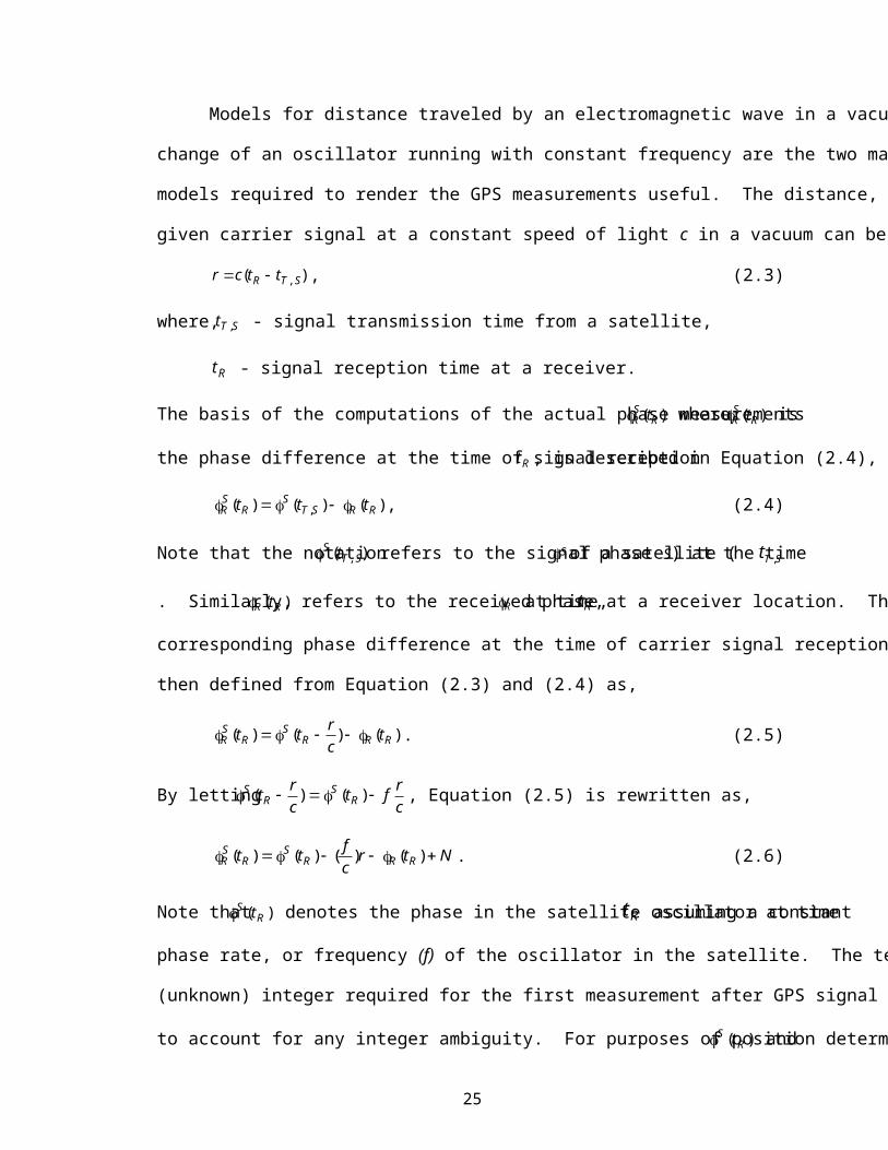
Models for distance traveled by an electromagnetic wave in a vacuum and the phase
change of an oscillator running with constant frequency are the two main mathematical
models required to render the GPS measurements useful. The distance, r traveled by a
given carrier signal at a constant speed of light c in a vacuum can be calculated as,
)( ,STR ttcr , (2.3)
where, STt , - signal transmission time from a satellite,
Rt - signal reception time at a receiver.
The basis of the computations of the actual phase measurements )( RSR t where )( R
SR t is
the phase difference at the time of signal reception Rt , is described in Equation (2.4),
)()()( , RRSTS
RSR ttt , (2.4)
Note that the notation )( ,STS t refers to the signal phase S of a satellite (S) at the time STt ,
. Similarly, )( RR t refers to the received phase, R at time, Rt at a receiver location. The
corresponding phase difference at the time of carrier signal reception at the receiver end is
then defined from Equation (2.3) and (2.4) as,
)()()( RRRS
RSR t
crtt . (2.5)
By letting crft
crt R
SR
S )()( , Equation (2.5) is rewritten as,
Ntrcftt RRR
SR
SR )()()()( . (2.6)
Note that )( RS t denotes the phase in the satellite oscillator at time Rt assuming a constant
phase rate, or frequency (f) of the oscillator in the satellite. The term N is an arbitrary
(unknown) integer required for the first measurement after GPS signal lock is achieved or
to account for any integer ambiguity. For purposes of position determination, )( RS t and
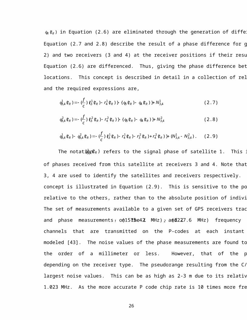
26
)( RR t in Equation (2.6) are eliminated through the generation of difference measurements.
Equation (2.7 and 2.8) describe the result of a phase difference for given satellites (1 and
2) and two receivers (3 and 4) at the receiver positions if their resulting equations from
Equation (2.6) are differenced. Thus, giving the phase difference between the two receiver
locations. This concept is described in detail in a collection of related subjects in [43, 45]
and the required expressions are,
14,343
14
13
14,3 )}()({)}()(){()( Ntttrtr
cft RRRRR (2.7)
24,343
24
23
24,3 )}()({)}()(){()( Ntttrtr
cft RRRRR (2.8)
)()}()()()(){()()( 24,3
14,3
24
23
14
13
24,3
14,3 NNtrtrtrtr
cftt RRRRRR . (2.9)
The notation )(14,3 Rt refers to the signal phase of satellite 1. This is the difference
of phases received from this satellite at receivers 3 and 4. Note that the numbers 1, 2, and
3, 4 are used to identify the satellites and receivers respectively. A “double difference”
concept is illustrated in Equation (2.9). This is sensitive to the position of one receiver
relative to the others, rather than to the absolute position of individual receiver locations.
The set of measurements available to a given set of GPS receivers tracking pseudorange
and phase measurements on the L1 (1575.42 MHz) and L2 (1227.6 MHz) frequency
channels that are transmitted on the P-codes at each instant have been mathematically
modeled [43]. The noise values of the phase measurements are found to be very small in
the order of a millimeter or less. However, that of the pseudorange vary significantly
depending on the receiver type. The pseudorange resulting from the C/A code has the
largest noise values. This can be as high as 2-3 m due to its relatively slow chip rate of
1.023 MHz. As the more accurate P code chip rate is 10 times more frequent, the resulting
27
noise level is as low as 10-30 cm. Greater accuracy requirement translates into a call for
additional improved and more sophisticated signals. This has been at the fore in the past
two years among the GPS communities. Two additional civilian carrier frequencies have
been proposed for the next batch of satellites, which is referred to as "Block IIF". These
new satellites are scheduled for launching beginning the year 2003 [118]. An
announcement by the U.S. Vice President, Albert Gore in a White House press release on
March 30, 1999, also confirmed developments in these new signals for civilian
applications. These are intended to further enhance the accuracy, reliability and the
robustness of civilian GPS receivers. With this, a more effective corrections for the
distorting effects of the Earth on GPS signals can be achieved.
2.4 Sources of Error and Correction
Perhaps the most often asked question about the GPS technology relates to its
accuracy. The ultimate accuracy of position measurements made using the GPS depend
on a variety of factors (e.g. the type of measurement made, x, y, or z, ionospheric and
tropospheric conditions, government inserted error effected as a security measure, number
of satellites in view, receiver equipment used, digital signal processing of the received
signal, surface features, reflection of signals and other factors).
A GPS receiver basically measures a raw one-way quantity (corrupted by user clock
bias) called pseudorange. This corrupted pseudorange measurements can be corrected for
atmospheric and other effects. With an approximate user location, the receiver can process
the corrected pseudorange (to four or more satellites) to determine location in the standard
GPS 1984 coordinate system referred to as the WGS-84 (1984 World Geodetic System)
[2, 5]. Various manufacturers have implemented the "anywhere" fix system that can start
28
from any location. The intentional timing distortion (i.e. SA) is randomly applied to the
GPS signal for civilian applications to reduce its ranging accuracy. This is probably one
of the main reason for the existence of differential GPS. It is possible that part of the
deliberate SA error is added to the satellite ephemeris. The pseudorange error growth due
to SA with an acceleration a and the age of correction (latency) t in seconds can be defined
by using motion dynamics theory as being approximately 25.0 at . Usually, the latency
st 40 . Typical SA acceleration is of the order of 4 10-3 m/s2 [43]. Consequently, the
pseudorange error ( 1 ) due to SA will grow to approximately 0.2 m if 10t s. GPS uses
atomic clocks (cesium and rubidium oscillators) which have stability of about 1 part in
1310 over a day. Note that at the time of press, the SA is believed to have been removed
by the United States government [119]. This could improve the GPS positioning
measurement accuracy given that no other adverse constraints are enforced to compromise
national security. This improvement is yet to be studied and quantified. Satellite clock
errors are differences in the true signal transmission time and the transmission time implied
by the navigation message. The ionosphere is known to be reasonably well-behaved and
stable in the temperate zones but could fluctuate considerably near the Equator or magnetic
poles [43]. GPS signals travel at a speed different from that of light as they transit this
medium in space. The modulation on the signal is delayed in direct proportion to the
number of free electrons encountered and inversely proportional to the square of the carrier
frequency.
A technique for dual-frequency precise-code receivers to correct ionospheric error
is to measure the signal at both L1 and L2 frequencies. The difference between the arrival
times of the L1 and L2 frequencies allows for a direct solution of any delay due to
29
ionospheric errors. Variations in temperature, pressure, humidity and, the presence of
water molecules (i.e., troposphere) all contribute to variations in the speed of light. Hence,
affecting the overall accuracy in the pseudorange measurements. Also, some of the signals
(indirect) can be delayed relative to the "direct" signal (i.e., multipath). The
aforementioned errors and their models are described in detail in [43, 50 and 51]. Various
methods including the DGPS have been developed to overcome the above mentioned
limitations in measurement accuracy. The DGPS mode is generally used to attenuate or
possibly, eliminate the SA error completely. The differential corrections can also be very
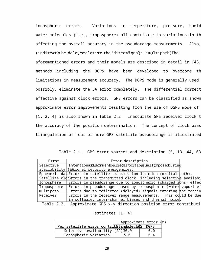
effective against clock errors. GPS errors can be classified as shown in Table 2.1. The
approximate error improvements resulting from the use of DGPS mode of measurement
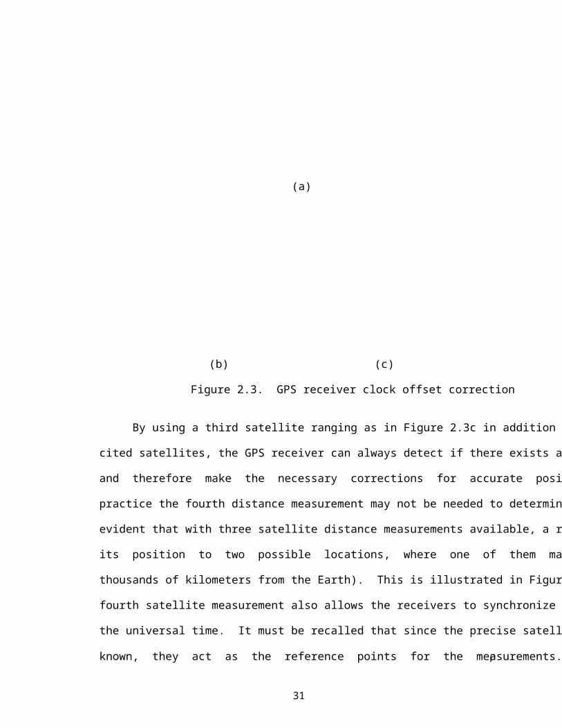
[1, 2, 4] is also shown in Table 2.2. Inaccurate GPS receiver clock time significantly affects
the accuracy of the position determination. The concept of clock bias correction using
triangulation of four or more GPS satellite pseudorange is illustrated in Figure 2.3.
Intentionally government applied distortion. Usually imposed during national security emergencies.
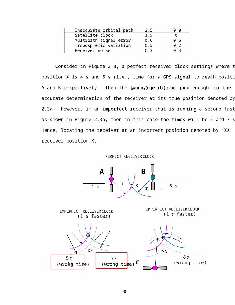
Ephemeris data Errors in satellite transmission location (orbital path). Satellite clock Errors in the transmitted clock, including selective availability. Ionosphere Errors in pseudorange due to ionospheric (charged ions) effects. Troposphere Errors in pseudorange caused by tropospheric (water vapor) effects. Multipath Errors due to reflected (delayed) signals entering the receiver antenna Receiver Errors in the receiver range measurements. This could be due to inaccuracy
in software, inter-channel biases and thermal noise. Table 2.2. Approximate GPS x-y direction position error contributing factors and
estimates [1, 4]
Approximate error (m) Per satellite error contributing factor Standard GPS DGPS
(*) See the “NovAtel Millennium GPSCard-Guide to Operation & Installation,” 1997.
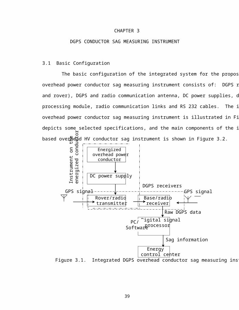
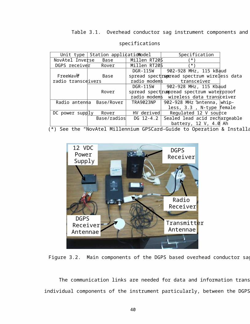
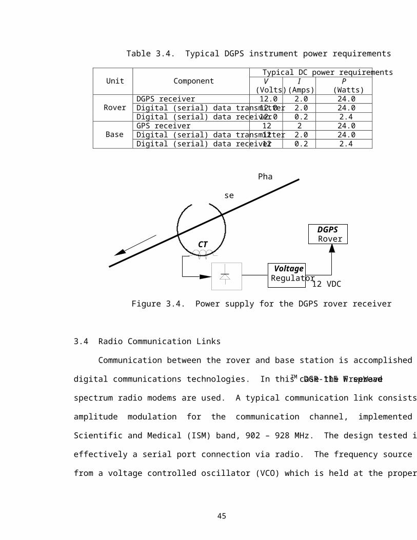
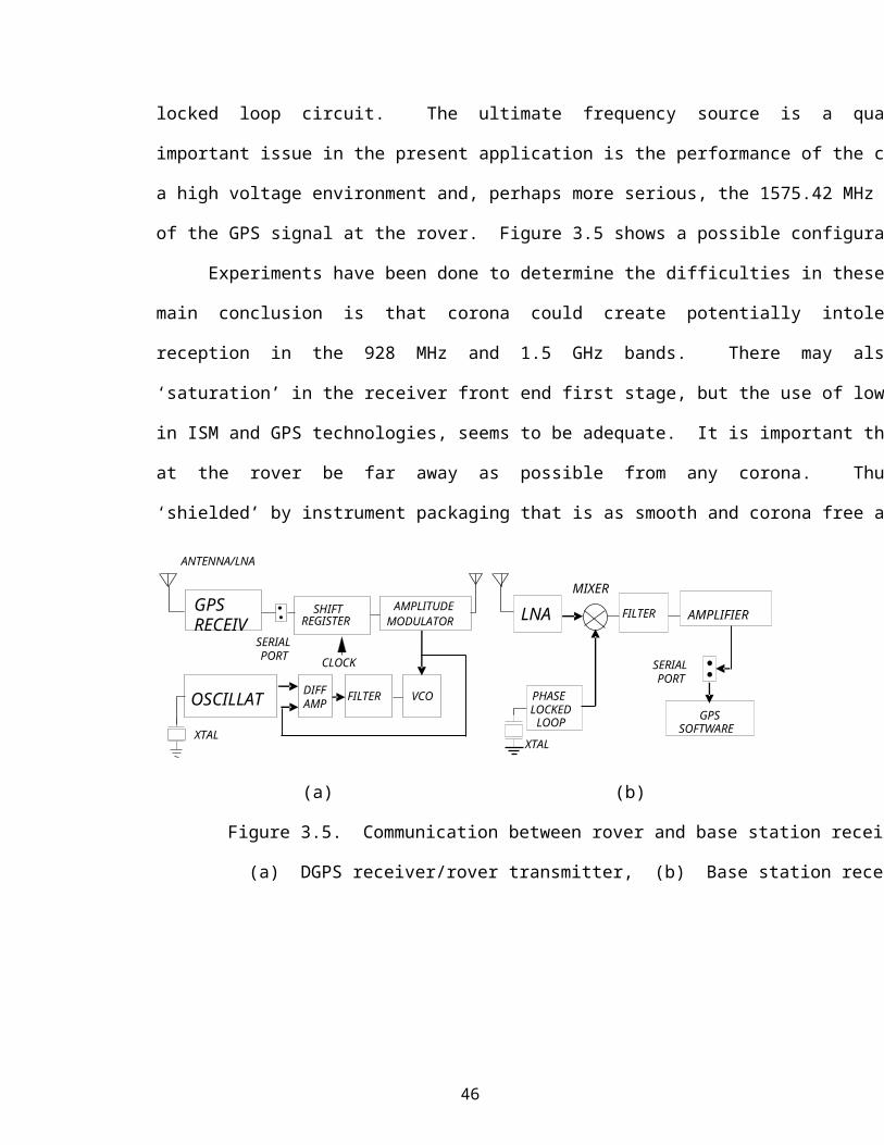
Figure 3.2. Main components of the DGPS based overhead conductor sag instrument
The communication links are needed for data and information transfers among the
individual components of the instrument particularly, between the DGPS receivers, and
Transmitter Antennae
Radio Receiver
DGPS Receiver
12 VDC Power Supply
DGPS Receiver Antennae
41
also to a designated control center for use by power system operators. The NovAtel DGPS
receivers and the FreeWave TM spread spectrum radio modems are energized by 12 VDC
power supply sources. The DGPS rover receiver is intended to receive DC power supply
which is derived from the overhead power transmission line. The NovAtel Millen RT20S
(i.e., real time 20 cm single frequency (1575.42 MHz)) DGPS receivers incorporates a
special software that allows for inverse DGPS operation. The inverse DGPS mode of
operation is proposed and this is outlined below. GPS signals are received simultaneously
by both the rover and base station receivers. The rover decodes the signals to determine
its approximate (i.e., before differential error corrections are made) position. The position
data are then transmitted to the base station DGPS receiver via radio receivers. The base
station DGPS receiver continuously applies the appropriate differential error corrections to
the received DGPS rover positioning message. With the error correction messages and
signal information from the GPS satellites, the rover which is attached to the overhead
conductor by design provides raw DGPS data which give an indication of the approximate
overhead conductor position (x, y, and z) at any given instance of time, t. This raw data is
then transferred to a DSP module (personal computer) via the base station receiver.
Further postprocessing of the data takes place at this stage to achieve the required
accuracy in the overhead conductor sag measurement by using appropriate DSP methods.
The resulting overhead conductor sag information is then transferred to a control center for
implementation. It is also possible to integrate this conductor sag information with existing
energy management system (EMS) modules. Some pictorial illustrations of the bench
testing setup at the APS Ocotillo power substation and a HV insulation laboratory at
Arizona State University (ASU) are shown in Appendix D.
3.2 Differential GPS Card
42
The DGPS receiver component consists of a DGPS antenna and cards
(GPSCardTM). Two main sections can be identified from the GPSCard TM module. These
are the RF (radio frequency) and digital sections. The digital section of the GPSCard TM
has three subsections, and these are the signal processor, the central processing unit (CPU),
and the system input/output (I/O). The signal processor contains two ASIC (application-
specific integrated circuit) correlator chips and an A/D converter. The CPU is the main
engine for all the system control, processing, and positioning intelligence. The I/O section
permits two-way communications and timing strobes between external data
communications equipment (DCE) and the GPSCardTM.
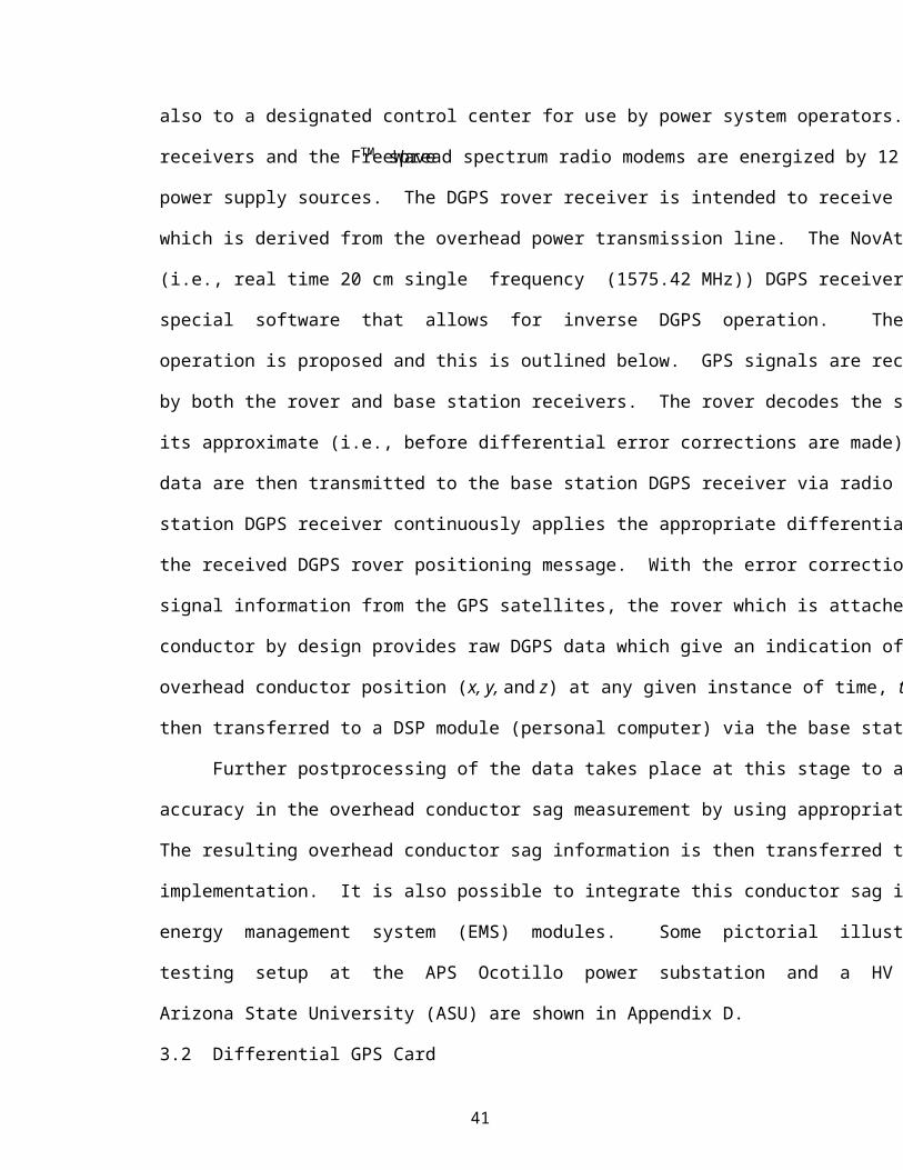
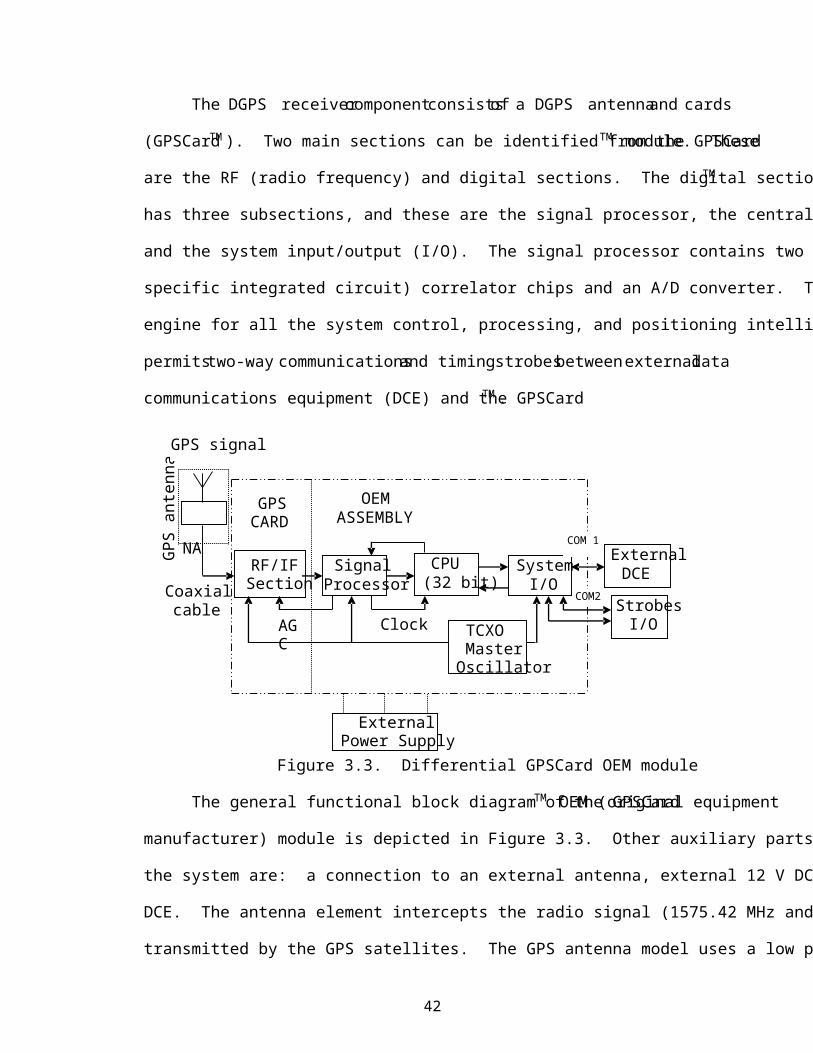
Figure 3.3. Differential GPSCard OEM module
The general functional block diagram of the GPSCardTM OEM (original equipment
manufacturer) module is depicted in Figure 3.3. Other auxiliary parts required to complete
the system are: a connection to an external antenna, external 12 V DC power supply and
DCE. The antenna element intercepts the radio signal (1575.42 MHz and/or 1227.60 MHz)
transmitted by the GPS satellites. The GPS antenna model uses a low profile microstrip
GPS
ant
enna
Signal Processor
RF/IF Section
CPU (32 bit)
System I/O
External DCE
L
NA
TCXO Master
Oscillator
External Power Supply
GPS CARD
OEM ASSEMBLY
Strobes I/O AG
C Clock
Coaxial cable
COM 1
COM2
GPS signal
43
technology with built-in LNA (low noise amplifier) and bandpass filtering. The intercepted
signal is then coupled to the LNA where it is amplified to overcome losses incurred by the
coaxial cable between the antenna and the GPSCardTM. The GPSCardTM receives the
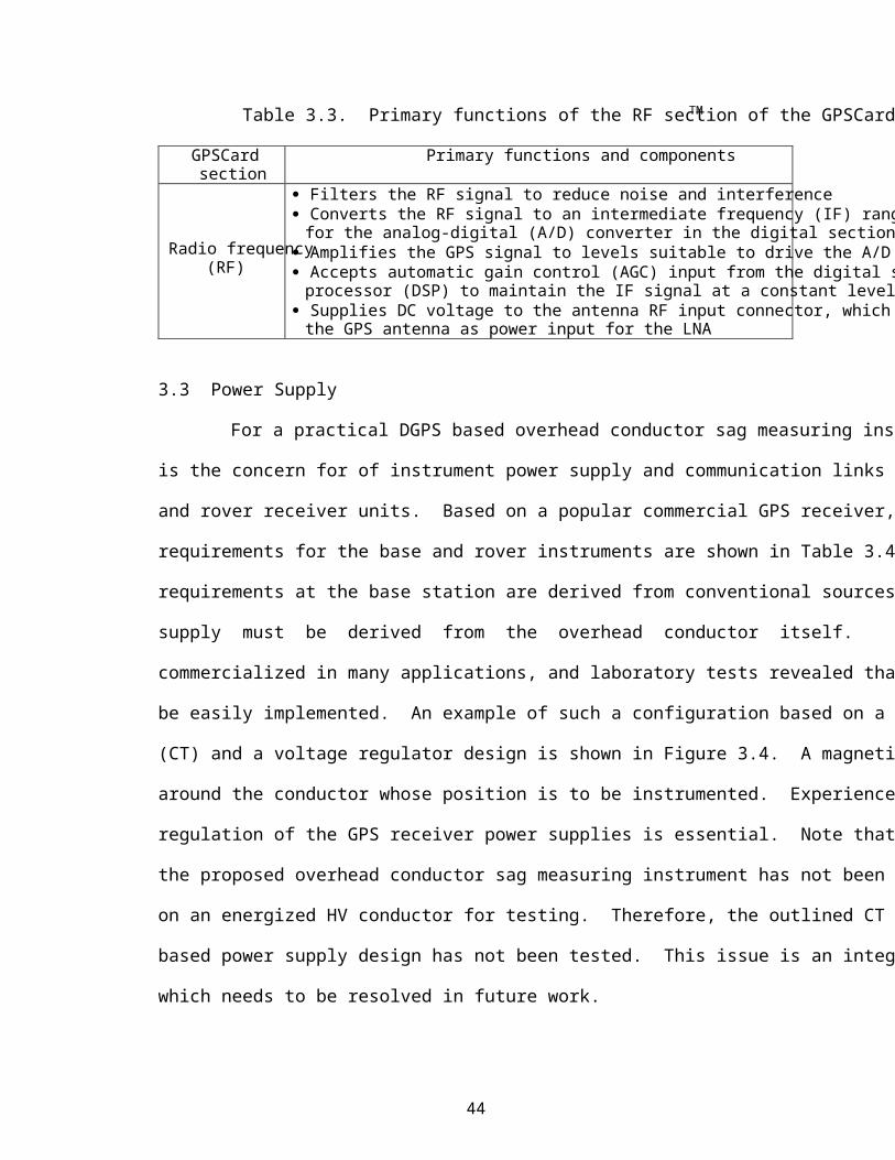
filtered and amplified RF signal from the GPS antenna. A summary of the sections,
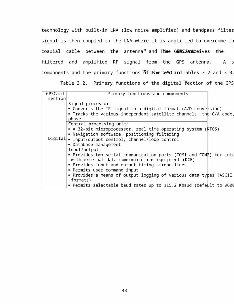
components and the primary functions of the GPSCardTM is given in Tables 3.2 and 3.3.
Table 3.2. Primary functions of the digital section of the GPSCardTM
GPSCard section
Primary functions and components
Signal processor: Converts the IF signal to a digital format (A/D conversion) Tracks the various independent satellite channels, the C/A code, and the carrier phase
Digital
Central processing unit: A 32-bit microprocessor, real time operating system (RTOS) Navigation software, positioning filtering Input/output control, channel/loop control Database management
Input/output: Provides two serial communication ports (COM1 and COM2) for interfacing
with external data communications equipment (DCE) Provides input and output timing strobe lines Permits user command input Provides a means of output logging of various data types (ASCII and binary
formats) Permits selectable baud rates up to 115.2 Kbaud (default to 9600 baud)
44
Table 3.3. Primary functions of the RF section of the GPSCardTM
GPSCard section
Primary functions and components
Radio frequency
(RF)
Filters the RF signal to reduce noise and interference Converts the RF signal to an intermediate frequency (IF) range suitable
for the analog-digital (A/D) converter in the digital section Amplifies the GPS signal to levels suitable to drive the A/D converter Accepts automatic gain control (AGC) input from the digital signal
processor (DSP) to maintain the IF signal at a constant level Supplies DC voltage to the antenna RF input connector, which is used by
the GPS antenna as power input for the LNA
3.3 Power Supply
For a practical DGPS based overhead conductor sag measuring instrument, there
is the concern for of instrument power supply and communication links between the base
and rover receiver units. Based on a popular commercial GPS receiver, the power supply
requirements for the base and rover instruments are shown in Table 3.4. The power supply
requirements at the base station are derived from conventional sources. At the rover, power
supply must be derived from the overhead conductor itself. This concept has been
commercialized in many applications, and laboratory tests revealed that the technology can
be easily implemented. An example of such a configuration based on a current transformer
(CT) and a voltage regulator design is shown in Figure 3.4. A magnetic ring is clamped
around the conductor whose position is to be instrumented. Experience shows that voltage
regulation of the GPS receiver power supplies is essential. Note that as of publication time,
the proposed overhead conductor sag measuring instrument has not been directly mounted
on an energized HV conductor for testing. Therefore, the outlined CT and voltage regulator
based power supply design has not been tested. This issue is an integral part of the work
which needs to be resolved in future work.
45
Table 3.4. Typical DGPS instrument power requirements
Unit
Component
Typical DC power requirements V
(Volts) I
(Amps) P
(Watts)
Rover DGPS receiver 12.0 2.0 24.0 Digital (serial) data transmitter 12.0 2.0 24.0 Digital (serial) data receiver 12.0 0.2 2.4
Base
GPS receiver 12 2 24.0 Digital (serial) data transmitter 12 2.0 24.0 Digital (serial) data receiver 12 0.2 2.4
Figure 3.4. Power supply for the DGPS rover receiver
3.4 Radio Communication Links
Communication between the rover and base station is accomplished using standard
digital communications technologies. In this case the FreeWave TM DGR-115 W spread
spectrum radio modems are used. A typical communication link consists of an ‘on-off’
amplitude modulation for the communication channel, implemented in the Industrial
Scientific and Medical (ISM) band, 902 – 928 MHz. The design tested in the laboratory is
effectively a serial port connection via radio. The frequency source in this design is derived
from a voltage controlled oscillator (VCO) which is held at the proper frequency by a phase
CT
Voltage Regulator
12 VDC
DGPS Rover
Pha
se
46
locked loop circuit. The ultimate frequency source is a quartz crystal (XTAL). An
important issue in the present application is the performance of the communication link in
a high voltage environment and, perhaps more serious, the 1575.42 MHz band reception
of the GPS signal at the rover. Figure 3.5 shows a possible configuration.
Experiments have been done to determine the difficulties in these areas and the
main conclusion is that corona could create potentially intolerable conditions for radio
reception in the 928 MHz and 1.5 GHz bands. There may also be some degree of
‘saturation’ in the receiver front end first stage, but the use of low noise amplifiers, standard
in ISM and GPS technologies, seems to be adequate. It is important that the radio receivers
at the rover be far away as possible from any corona. Thus, the receiver should be
‘shielded’ by instrument packaging that is as smooth and corona free as possible.
(a) (b)
Figure 3.5. Communication between rover and base station receivers
(a) DGPS receiver/rover transmitter, (b) Base station receiver
GPS RECEIV
SERIAL PORT
SHIFT REGISTER
AMPLITUDE MODULATOR
CLOCK
OSCILLAT DIFF AMP FILTER VCO
XTAL
ANTENNA/LNA
LNA
SERIAL PORT
MIXER FILTER AMPLIFIER
GPS SOFTWARE
PHASE LOCKED LOOP
XTAL
47
3.5 Laboratory Bench-Testing and Substation Experiments
A selected number of experiments were performed on the DGPS based overhead
conductor sag measuring instrument at different environmental conditions. The main
objectives of the bench-testing experiments were to evaluate the proper functioning of the
radio communication links, assess the GPS satellite signal reception capabilities, and to
also attest the behavior of the instrument under HV environment. In this case the
experiments were performed at the High Voltage Insulation Laboratory in the Engineering
Research Center (ERC) building, Room 588 and also on the roof top of the same building
at Arizona State University, Tempe. Other similar experiments were also performed at the
APS Ocotillo power substation in Tempe, Arizona at about 14 ft directly under 230 kV
lines (i.e., approximately 0.3112 kV/cm electric field strength). Some of the results of the
selected experiments tested are outlined in Tables 3.5 and 3.6. In Tables 3.5 and 3.6 a
“Yes” satellite signal reception implies that enough number of satellites (usually 6 satellites
or more) were received and a rover receiver position was computed. Similarly, a “No”
condition represents a scenario whereby the DGPS system was found to be operating
properly but was not able to compute the rover receiver position due to satellites not being
visible at the time of the experiment. In all the experiments performed there were no
problems found with the radio receiver operation.
Note that in these experiments, the proposed DGPS based conductor sag instrument
was not directly mounted on an energized overhead HV conductor due to lack of logistics
and high cost in terms of the availability of necessary facility. To be able to perform such
an experiment in a real life application is beyond the capability of the university research
resource at this time. However, this concern is an issue to be considered in collaboration
with industry for possible prototype improvement and commercialization. A selected
48
pictorial set up for some of the experiments performed in this work are shown in Figures
3.6 and 3.7.
Table 3.5. Selected results of bench-tests performed at ASU HV laboratory using
conventional 12 VDC power supplies
Tests performed to evaluate the proper functioning of the radio communication links, GPS signal reception and attest the behavior of the instrument under no HV and HV
conditions
Testing location
Environ-mental
condition
Approximate computed
electric field strength (kV/cm)
Data
transfer link
Number
of satellites received
Signal reception
radio link
DGPS base to rover
ERC building (roof-top)
No HV 0.0 Hard wired
5-9 Yes Yes
ERC building (roof-top)
No HV 0.0 Radio receiver
5-9 Yes Yes
ERC building (HV Lab Room 588)
HV 0-0.8 Hard wired
0 Yes No*
ERC building (HV Lab Room 588)
HV 0-0.8 Radio receiver
0 Yes No*
(*) Tests done indoors and no satellites were visible
Table 3.6. Results of experiments conducted at the APS Ocotillo power substation in
Tempe, Arizona on 7/7/2000 using conventional 12 VDC power supplies
Tests performed to evaluate the proper functioning of the radio communication links, GPS signal reception and attest the behavior of the instrument under no HV and HV
conditions
Testing location
Environ- mental
condition
Approximate
computed electric field strength
(kV/cm)
Data
transfer link
Number
of satellites received
Signal reception
Radio link
DGPS Base to rover
Power substation
(APS)*
Directly under energized
lines
0.3112 Hard wired
5-9 Yes Yes
Power substation
(APS)*
Directly under energized
lines
0.3112 Radio receiver
5-9 Yes Yes
(*) Tests performed at approximately 14 ft directly under 230 kV lines. Enough satellites were received with no detection of radio link problems
49
Figure 3.6. Experimental setup at the APS Ocotillo power substation in Tempe, Arizona
on 7/7/2000 to evaluate prototype functioning and GPS signal reception
Figure 3.7. Experimental setup at an ASU HV insulation laboratory in Tempe, Arizona
on 3/7/2000 to evaluate prototype functioning and GPS signal reception
3.6 Financial Estimates of DGPS Conductor Sag Instrument
Integrated DGPS Rover Component Prototype
Nytech Power Donut
50
Table 3.7. Estimated cost of selected inverse DGPS instrument components
DGPS station unit type
Inverse DGPS unit model
Selected specifications Unit price (US$)
Base receiver NovAtel MiLLen-RT20S/Powerak-II
(OEM2-3111R*)
Millennium real time kinematic phase positioning, 20 cm, single frequency
5,665.00
(2,995.00*)
Rover receiver NovAtel MiLLen-RT20S/Powerak-II
(OEM2-3111R*)
Millennium real time kinematic phase positioning, 20 cm, single frequency
Rover package* Modified power donut 500.00 1000.00 5000.00 50000.00 Rover
installation* Safely secured on HV
lines 1000.00 2000.00 10000.00 10000.00
Tentative estimated total cost in US$ 17226 26189 97893 904563 Tentative estimated cost per unit in US$ 17226 13095 9789 9046
(*) Approximate costs, (**) Approximate costs excluding PC
52
3.7 Preliminary Conclusions and Main Challenges
Field trial testing conducted in a laboratory and power substation environment
in Tempe, Arizona indicates the feasibility of GPS signal reception for measurements taken
at about 14 ft directly below 230 kV lines. The existence of corona discharges may affect
the normal operation of the DGPS based conductor sag measuring instrument, together
with the communication links used for data transfers however, no rover - base radio
communication problems were observed for the 900 MHz technology tested. The main
conclusions drawn from bench and substation testing are described in Table 3.9. The
NovAtel real time kinematic positioning Millennium (MiLLen RT20S) DGPS OEM
receiver series that are capable of inverse DGPS operation are recommended for a
commercialized working model of the DGPS based overhead HV conductor sag measuring
instrument. This allows for the computed conductor sag data to be accessible at the base
receiver location (e.g., energy control center).
Table 3.9. Main conclusions drawn from laboratory and power substation tests
Conclusions Comments DGPS measurements Field trials confirm the feasibility of the application
Power supply and communication links
An outline of a plausible design are already in place
Potential source of inaccuracy
Inaccuracies in the exact location of DGPS antenna sensor Inexact coordinates for the surveyed DGPS base station receiver
Power supply Derived from conventional DC power sources for the base station and radio transceivers. Rover power supply, based on a CT design is derived from the energized overhead conductor power
Communication links Consists of "ON-OFF" amplitude modulation Serial port connection via radio Frequency range of 902-928 MHz (ISM band) Reliable data transfer capabilities
Rover unit packaging Utilizes a modified Power Donut model as an enclosure Components include NovAtel DGPS cards, radio communication
equipment, derived power supplies and external antenna Equipment to be packaged as corona free as possible Use commercially available weather proofing solutions
Commercial prototype Expert construction and possible subcontracting recommended
53
CHAPTER 4
SIGNAL PROCESSING OF DGPS SAG INSTRUMENT DATA
4.1 Introduction
The essence of the GPS technology is a receiver clock offset and 3-D position of
GPS receivers which are determined from measured satellite-to-receiver ranges called
pseudorange. The pseudorange is based on 4 or more GPS satellite signal reception.
Evidence about the error in raw DGPS measurements has been reported since the inception
of the technology over two decades ago. The measurement errors can be traced to various
sources including SA, multipath, ionospheric, tropospheric effects and, clock offset [3, 4,
5] as discussed in chapter one. SA error of 0.2 s (60 m) is not unusual. In addition, errors
due to the propagation of the signals from GPS satellites, solution of the system of
pseudorange equations and others also occur. DGPS vertical (z) measurement errors in the
order of 15 m and beyond are not unusual in some applications. In order to improve the
measurement accuracy, postprocessing of the DGPS measurement data using appropriate
engineering and digital signal processing (DSP) tools is often therefore inevitable.
The present chapter focuses on the DSP of DGPS measurement data. A
methodology for further improving DGPS altitude measurements accuracy has been
described. The resulting information will be used to accurately determine high voltage
(HV) overhead conductor sag. For this reason, various signal processing methods namely:
bad data modification, LSPE, ANNE, and a combination of these methods as well as Haar
wavelet transforms have been considered as a postprocessing technique to further improve
the accuracy of the raw DGPS measurements [42, 59, 60, 61, 83, 84, 85, 87, 88, 95, 96,
97].
54
4.2 Preliminary Field Trials and Data Analysis
A Differential GPS receiver prototype was initially assembled around the NovAtel
2111R GPS engine by Hunt and Yancey [6] for preliminary GPS measurement data
collection and experimentation. The system consists mainly of a ten-channel NovAtel GPS
card, a power supply, radio links between the DGPS receiver stations, and software to
resolve the position of the rover position. Appendix D shows some of the various
components and environment used for the various experiments. This experimental set up
was used to preliminary assess the feasibility of the project. The initial GPS measurement
data were collected under various environmental conditions at a location adjacent to the
SRP (Salt River Project) substation in Tempe, Arizona [6], using the 2111R GPS
prototypes. Three separate experimental cases were considered, and these are shown in
Table 4.1. These data were analyzed by the present author to evaluate the accuracy levels
of DGPS measurements over that of standard GPS, and to also determine the effects of
high voltage fields on the measurements taken. Some of the results of the data analysis are
shown in Figures 4.1 through 4.6. In case “C”, the measurements were taken at
approximately 18 ft directly below the center conductor of 230 kV lines. Thus, under
electric field strength of approximately 0.2420 kV/cm.
Table 4.1. Case study for preliminary measurement data analysis
Case Method of signal reception Environmental conditions A GPS Non-HV environment B DGPS Non-HV environment C DGPS Approximately 18 ft under 230 kV
overhead lines (0.2420 kV/cm) The main computer software used were the NovAtel "gpsoln", Microsoft Excel and
MATLAB applications. The GPS receivers were employed in the stationary position
55
during the data collection. These initial measurements were not intended for an actual
overhead conductor sag measurement, but rather, to become familiar with the DGPS
hardware and software, and to also validate the applicability of the DGPS technology in
terms of accuracy for the application under consideration. Figures 4.1 through 4.6 are the
postprocessed data showing distribution and time variations of the altitude measurements
taken under various set of environmental constraints. Statistical analysis of the resulting
data using the Microsoft Excel software is depicted in Table 4.2. It shows a comparison
of GPS and DGPS measurements of the initially assembled instrument in terms of altitude
above ellipsoid (vertical position) under controlled conditions. The data was based on field
trials of over 3500 s of measurements. It is to be noted that the measurements were for the
purpose of illustrating the accuracy improvement using DGPS. The reference
measurements used to evaluate the attained improvements of the measured DGPS data are
shown in Figures 4.1 and 4.2. These were taken in an open area in the absence of both
overhead HV conductors and DGPS corrections (i.e., case “A”). These data indicated a
weakness of GPS in the altitude measurements. A variation of about 190 m in the
measurements taken over a two-hour period was observed. The second set of measurements
as shown in Figures 4.3 and 4.4 were taken under the same set of conditions as above but,
with DGPS corrections (i.e., case “B”) at a receiver separation distance of 18 ft (5.49 m).
The DGPS data in Figure 4.3 showed a substantial improvement in accuracy over the same
period of field trials hence, proving the feasibility of the research project at hand. The
standard deviation, is 3.14 m as compared to 33.55 m in Figure 4.1. These measurement
data were used to verify any performance difference with the data taken in the presence of
the 230 kV environment.
56
Table 4.2. Statistical analysis of raw GPS and DGPS measurements of altitude (z) above
ellipsoid under controlled conditions
Statistical Statistical distribution in meters Raw measurement in meters parameter Case A Case B Case “C”
34.55 4.14 1.79 x 372.07 372.32 359.69
median 372.53 372.11 359.72 mode 386.00 372.11 358.77
Figure 4.1. GPS distribution in the vertical (z) direction [Case “A”]
1981 Revised Rating (Unspecified probability level,
assumed life 25 years) Summer Winter Summer Winter Air temperature 40oC 10oC 35oC 10oC Wind Speed 2 ft/s 2 ft/s 3 ft/s 3 ft/s Normal (95oC) 970 A 1240 A 1101 A 1347 A LTE (115oC, 3 hrs) 1140 A 1370 A 1270 A 1476 A STE (125oC, 15 min) 1310 A 1520 A 1430 A 1616 A
84
The temperature of the overhead conductor can be determined after having obtained
an accurate conductor sag measurements by using the critical span sag-temperature
relationship. Equation (5.10) gives a close approximation of temperature as a function of
the overhead conductor sag,
432 )()()()( icicicicic SSDSSCSSBSSATT , (5.10)
where in Equation (5.10), Tc is the computed present conductor temperature, and T i is that
of an unenergized conductor replica. S c and Si, are respectively the corresponding
conductor sags. The calibrated parameters A, B, C and D can be determined empirically
by using various temperature and conductor sag measurement together with curve fitting
techniques [15]. Thus, these constants are determined under controlled conditions with
known Ti and Si. The values of the temperature, Ti can be measured using available
instruments for known conductor sag values Si. The conductor sag can be derived from the
real time measurements of the DGPS conductor sag instrument which can then be used to
determine the conductor temperature and hence, the permissible conductor loading for
operational purposes. An expression for a third degree approximation of Equation (5.10)
has been proposed by T. O. Seppa et al., and the conductor ampacity is then computed
using Equation (5.11) [15]. However, this equation is an empirical relationship which the
present author has not validated. Note also that the validity of IT is dependent on the
accuracy of determining the parameters in Equation (5.8).
oc
omTM TT
TTII
, (5.11)
Mp IVS 3 ,
where IM = ampacity at maximum allowable conductor temperature, [A]
IT = ampacity to limit conductor to the computed temperature, [A]
85
Tc = computed conductor temperature [oC]
Tm = maximum allowable conductor temperature [oC]
T0 = actual ambient temperature, [oC]
Sp = apparent power, [MVA].
Note that due to the stochastic nature of ambient conditions, a conductor replica as
proposed by Seppa et al is used to determine the actual ambient temperature, T0 and the net
radiation This mathematical model (5.11) has been the basic tool in many applications for
the determination of dynamic thermal ratings of overhead conductors. An example of how
this model is used to calculate the allowable ampacity level of overhead HV conductor,
specifically a 230 kV ACSR "Drake" is illustrated in [15]. Ultimately, the results obtained
in this respect for a given condition could be used for on-line system study, and to also
estimate the ratio of the change in conductor sag, Sc and conductor current, I (i.e., ISc /
) for anticipatory purposes. Based on the temperature- sag model, typical line loading
information may be transmitted to the systems operator via an appropriate communications
device. This may include the present safe conductor loading levels, and more importantly,
the amount of load that must be reduced to achieve the required safe loading level. The
concept is summarized in Figure 5.6.
Figure 5.6. Block diagram for conductor ampacity rating calculation
GPS
Signal Postprocessed
DGPS Measurements
Equation (5.10)
Equation (5.11)
Systems Operator
Sag Temp.
Rating
System study
86
5.5 Determination of Maximum Transfer Capacity
In a competitive deregulated electric power industry any electric consumer should
be able to purchase power from any generating company. This results in two generic
transmission issues: the first is the problem of obtaining circuit capacity for point-to-point
transmission, and the second is the development of transmission service from a control area
to a point. In order to preserve system reliability, the “n-1” type of line contingency study
is done. Consequently, a method known as the maximum steady state load increase
(MSSLI) [20] at a specific bus is considered under this section. The method is iterative
and based on the linearization of system operation near high levels of operation. The “n-
1” contingency (line outage) security consideration is included in the calculation. This
may be used as an index to assess the steady state transmission capacity between regions
in an interconnected power system. This concept can also be extended to include the DTLR
case for a given conductor temperature and ambient conditions, and the same algorithm
used for the MSSLI simulations are also therefore applicable.
The MSSLI is defined to be that value of load increase at a given bus for a steady
state condition that makes the loading in any line of the system reach rated value when
considering the most severe first (i.e., “n-1”) contingency. To start with, the initial
conditions of the problem are set based on a load flow study. The initial load flow study
represents the actual steady state operating point of the system. The bus susceptance matrix
Bbus is also formed. The corresponding linear sensitivity factors (i.e., generation shift and
line outage distribution) are computed based on the elements of the susceptance matrix.
The generation shift factor, lia which represents the sensitivity of power flow on line l to
a change in generation at bus i is defined as follows:
87
i
lli P
fa
. (5.12)
where l, i = line and bus indices respectively
Pi = change in generation at bus i
fl = variation of power flow on line l when a change in generation, Pi occurs at bus i.
It is assumed in Equation (5.12) that the change in generation, Pi is exactly compensated
by an opposite change in generation at the swing bus with all other generators remaining
fixed. As shown in [93] the complex generation shift factor is described as,
*,,*
1mibusnibus
lli ZZ
za (5.13)
where (*) denotes complex conjugation and,
i - generator bus index other than the reference bus
n, m - bus indices corresponding to line l
zl = rl +jxl - line impedance of line l (from index n to m)
Zbus, ni and Zbus, mi - entries in the Zbus matrix referenced to the swing bus.
The complex notation in Equation (5.13) can be dropped to obtain the approximate line
megawatt (i.e., active) power flows. By so doing the generation shift factor, ali then
becomes purely real, where the Xbus matrix is the imaginary part of the bus impedance, Zbus
matrix.
minil
li XXx
a 1 (5.14)
Similarly, the line outage distribution factors are,
ok
lkl f
fd , (5.15)
88
where,
dl,k = distribution factor for line l after line k is outaged
f ok = original power flow on line k before being outaged (opened)
fl = variation in megawatt power flow on line l due to the outage of line k.
The Xbus matrix is formed by inverting the B’ bus susceptance matrix with the reference
bus elements removed, and then later including zeros in the row and column corresponding
to the reference bus. The power transfer distribution factor (PTDF) may also be defined
by Equation (5.16) where, neither i nor j is the swing bus,
nmmmnnk
jmimjninl
k
kl XXXx
XXXXxx
d2,
. (5.16)
In Equation (5.16), all real notation is used as before to estimate the megawatt power flows.
A shift in generation and load at all buses is required by the sale of power. The shift at the
buses is dependent of the way the extra load is going to be served, (i.e. either from point-
to-point or from control area-to-point). For point-to-point calculations, there will be load
rescheduling only at the two specified buses. For control area-to-point calculations, a
generation redispatch is required. In this dissertation work, a redispatch proportional to
the generator ratings, often referred to as participation “a” factors is adopted [41, 93]. Once
the generation and load shift at buses have been calculated, the new power flow on each
line in the network is computed using a pre-calculated generation shift factors,
i
ilio
ll Paff )(ˆ . (5.17)
where, lf = flow on line l after failure of a generator on bus i
olf = flow prior to the generator failure.
The MSSLI is found iteratively, advancing load level in steps until a system
circuit reaches its rating. This method identifies the line(s) which has reached its capacity,
89
as well as the corresponding load levels of the entire system. Figure 5.7 shows the MSSLI
algorithm used. In Figure 5.7 the circuits DTLR are proposed for use as Prated.
Figure 5.7. Algorithm for MSSLI index
The use of dynamically updated circuit ratings will allow the full use of
transmission circuits nearly in real time. In this way circuit capacity may be marketed to
interested entities, and circuits may be more fully used by the operating transmission
Initialize with
existing
conditions
Calculation of Pbus
at all buses
Correct Pbus
NO
Pmax Pbus
(n-1) contingency
analysis
Pline Prated
Report Pline
YES
YES
NO
MSSLI estimation at desired bus
Point-to-point or Control area-to-point
Increase Pbus
90
company. An illustrative example is developed to indicate how the calculation of MSSLI
is done. For this purpose, a six bus example is used as shown in Figure 5.8. The
corresponding system data are listed in Tables 5.2 and 5.3. The illustrative studies are
presented here in three cases: a base case (i.e. initial load flow) study, an illustration of
point-to-point MSSLI calculation, and finally a control area to point calculation of MSSLI.
Note that with the accurate monitoring of line loading under actual weather
conditions, it is expected that the thermal line ratings will be improved in comparison to
the steady state case. Therefore, the line rating characteristics can be perturbed to
accommodate the supposed improvement in line loading due to DTLR. The same
simulation algorithm used for the MSSLI case is therefore applicable to the DTLR case.
Hence, in order to avoid repetition, the results of the DTLR case is not shown in this
work. However, the DTLR simulation results indicated a better conductor loading
performance over the steady state ratings.
Under the assumed base case operating conditions, an outage analysis is done to
determine the possibility for an increase in load. Having found that there is no circuit
rating violation, a possible load demand increase at Bus 4 is studied. The second study is
a point-to-point study: the load increase at Bus 4 is going to be served exclusively from
the generator at Bus 2. A tentative value of 0.1 per unit (p.u.) load increase resolution is
used to initialize the problem, with posterior increases of 0.1 p.u. applied to the load until
a line rating is reached. The results are presented in Table 5.4.
91
Figure 5.8. Six-bus system illustration of MSSLI concept
Table 5.2. Line characteristics for the six-bus system
limits, effect of tap changers, generator power factor limits and system stability limits.
From the point of view of circuit ratings, dynamic (i.e., real time) thermal line ratings can
be easily included in the MSSLI calculation for a given future loading conditions. It is also
possible to include the study of short term (emergency) limits.
CHAPTER 6
95
CONCLUSIONS AND FUTURE WORK
6.1 Conclusions
In this dissertation work, the main consideration is to measure the overhead HV
conductor sag. The resulting conductor sag information can be used to enhance the
operation of electric power systems, particularly the DTLR. The proposed DGPS based
measurement of overhead HV conductor sag is a more direct technique in some ways as
compared to similar alternative methods. This is concluded because the direct
measurement of overhead conductor position involves no intermediate calculations and
measurements of conductor tension, temperature, ambient weather conditions, or make any
assumptions to that effect. A prototype has been constructed and tested under non HV and
HV environment. The main conclusions of this dissertation work can be categorized as
follows:
Design and construction of a prototype DGPS based overhead conductor sag
measuring instrument
Perform a selected number of non HV and HV environment laboratory bench and
power substation tests
DSP of DGPS based conductor position measurement data for data analysis and
accuracy enhancement
A proposed outline of a framework for the integration of DGPS based overhead
conductor sag information with DTLR
The main contributions of this research work is the proposal of an innovative concept
that is based on the use of precision DGPS technology to directly and accurately measure
96
the overhead conductor sag in real time. This proposal is the first of its kind in the utility
industry in regards to direct overhead conductor sag measurement. The net result of the
overhead conductor sag measurements proposed in this work incorporates the combined
effect of solar radiation, wind speed and direction, conductor loading in terms of electric
current, and all other effects that are otherwise difficult to measure individually. The
pertinence of the proposed work is to improve the emergency (n-1) line outage contingency
capability, increase power systems network reliability, and also to possibly influence the
sale of electric energy via OASIS. The method presents immediate promising benefits in
terms of pecuniary and reliability considerations, especially in the contemporary
deregulated electricity power market. This may consequently lead to some possible
transmission system investments deference.
Furthermore, the DGPS based conductor sag data should be reliable under normal
operational conditions of the overhead power conductor on which the rover is to be located.
It is to be noted that a great deal of care must be taken in the design of the instrument
packaging because of the potential possibility of electromagnetic interference from corona
discharges. The main advantage of the concept is that of the real time direct measurement
of a parameter (i.e., conductor sag) needed for the operation and enhancement of the HV
transmission system. It also presents a potential source for cost reduction and better
accuracy in the conductor sag measurement, since there is no need to directly measure
conductor tension, temperature and weather conditions. There are also several potential
disadvantages of the proposed DGPS method. These include costs, insufficient experience
with the technique and performance in a HV environment. However, the real time direct
measurement of overhead conductor sag is a clear advantage. The requirement of a second
DGPS receiver and corresponding communication equipment between the base and rover
97
instruments are also some of the drawbacks of the technique. Furthermore, spatial
correlation of atmospheric delays could cause the DGPS position accuracy to deteriorate
with increasing distance between the reference and the rover receivers. Typical accuracy,
limitations, strengths and weaknesses of the method are described. Present field trial
results of the DGPS based conductor position measurements, together with the DSP
methods utilized, confirm the feasibility of the proposed application. Some of the main
strengths and weaknesses of the proposed instrument and method are shown in Table 6.1.
Table 6.1. Strengths and weaknesses of the DGPS based sag measuring instrument
Strengths of the method
The concept is a more direct method in some ways as compared to similar alternative methods
Intermediate calculations or assumptions regarding ambient weather conditions, conductor temperature and tension measurements are not required
Potentially accurate and cheaper cost Capable of real time operation The accuracy of the proposed concept is pivoted on the
precise GPS timing signals and further DSP methods Removal of SA may further improve measurement
accuracy
Weaknesses of the method
Has not been tested directly on an energized HV line Uncertainty in cost, lack of sufficient experience with the
technique, and performance in HV environment Requires a second or several other DGPS rover receivers,
and corresponding communication equipment between the base and rover instruments
Prototype requires corona-free packaging Spatial correlation of atmospheric delays may cause the
DGPS position accuracy to deteriorate with increasing distance between the base and rover receivers
98
6.2 Main Research Contributions
The main contribution of this dissertation research is the design, construction, field
testing and analysis of a DGPS based instrument for the real time direct measurement of
overhead HV conductor sag. The integration of this instrument into system operation is
described. Practicalities and requirements of the instrument power supply, radio
communication links, DSP, and packaging are also given.
A secondary contribution includes a review of GPS and DGPS methods in power
engineering, DTLR, and related technologies. Also, a proposal is outlined for the
conductor sag data to be used for DTLR purposes. With regards to the contribution in DSP
of instrument measurement data, the raw DGPS measurement accuracy in the vertical
direction has been enhanced using DSP techniques such as bad data identification and
modification, LSPE, ANNE, and Haar wavelet transforms. An absolute error of about 17.2
cm for up to 70% confidence level has been achieved. The present results confirm that the
proposed DGPS based overhead conductor sag measuring instrument is feasible for the
direct instrumentation of overhead power conductor sag.
The MSSLI method to calculate the maximum incremental power loading at certain
bus points of an interconnected system has been proposed as a steady state indicator of
system transmission capacity. It is based on the use of linear sensitivity factors and
emergency (n-1) line outage contingency analysis. With this method, the critical lines of
the electric power network may be identified based on line loading capacity limits. The
method can be used for point-to-point or control area-to-point transmission capacity
analysis, and it can also be extended to include the DTLR case.
99
6.3 Recommendations for Future Work
The goal of future work has three main phases, and these are:
Construction and packaging of an integrated working model that is suitable for
operation on an energized overhead HV conductor
Comprehensive field testing of the packaged prototype in collaboration with
utility industries to evaluate the viability of the method, assess the measurement
accuracy under HV environment and possible requirements for
commercialization
Methodology to integrate the measured real time DGPS based overhead
conductor sag information with on-line DTLR applications
In this work the NovAtel 3111R DGPS receivers were used. However, the NovAtel
MiLLen (Millennium) RT20S DGPS receivers that are capable of reverse DGPS operation
are recommended for the reverse DGPS operation. The main challenges remained to be
solved in this work (prototype construction and testing) for a successful project
implementation can be expanded in the directions as shown in Table 6.2.
Table 6.2. Future work for project implementation
Tasks DGPS device packaging including integration with communication links Continuous power supply to the DGPS rover receiver is to be derived from the same HVAC
transmission line on which the receiver is located Evaluation of the effects of corona and other characteristics such as electromagnetic field
strength on the normal operation of the DGPS instrument Field testing of a packaged-prototype in an energized conductor environment) Evaluate the influence of the possible removal of SA Evaluate the measurement accuracy of the overall integrated prototype device Utilization of the DGPS based conductor sag data for DTLR, and its integration with OASIS
and system studies
100
The following must also be taken into consideration to evaluate the prototype DGPS
based conductor sag monitoring instrument under actual conductor and prototype operating
conditions for effective implementation:
The functional specifications for the hardware should include, but not limited to,
descriptions of environmental conditions under which it should operate,
accuracy, reliability, derived power supply, data storage, installation and
communication requirements.
The functional specifications of any additional software to be used must address
user interfaces, data transfer, analysis, and storage capabilities, computing
requirements, security, adaptability, and equally important is the features needed
for DTLR, and to also conduct line capability studies using information from the
[70] R. O. Burnett Jr., M. M. Butts, T. W. Cease, V. Centeno, G. Michel, R. J. Murphy,
A. G. Phadke, “Synchronized Phasor Measurements of a Power System Event,”
IEEE Transactions on Power Systems, Vol. 9, No. 3, August 1994, pp. 1643-1650.
[71] G. A. Bates, “The Use of GPS in a Mobile Data Acquisition System,”
Developments in the Use of Global Positioning Systems, 1994, pp. 2/1-2/3.
[72] P. Crossley, “Future of the Global Positioning System in Power Systems,”
Developments in the Use of Global Positioning Systems, 1994, pp. 7/1-7/5.
[73] J. A. Jodice, S. Harpham, “End-to-End Transient Simulation for Protection System
Performance Testing,” Developments in the Use of Global Positioning Systems,
1994, pp. 6/1-6/5.
[74] R. E. Wilson, J. A. Justers, “International Time Keeping for Power System Users,”
Sixth International Conference on Developments in Power System Protection (IEE
Conference Publication No. 434), March 25-27, 1997, pp. 351-354.
[75] M. Lillian, S. I. Thompson, “GPS Satellite Synchronized Test Systems Recreate
Fault Conditions to Troubleshoot Protective Relay Schemes,” Sixth International
110
Conference on Developments in Power System Protection (IEE Conference
Publication No. 434), March 25-27, 1997, pp. 346-350.
[76] E. P. Southern, H. Y. Li, P. A. Crossley, “GPS Synchronized Current Differential
Protection,” Sixth International Conference on Developments in Power System
Protection (IEE Conference Publication No. 434), March 25-27, 1997, pp. 342-345.
[77] A. Dierks, I. Worthington, P. Olivier, P. “GPS Synchronized End-to-End Tests of
Transmission Line Teleprotection Schemes in the ESKOM Networks,” Sixth
International Conference on Developments in Power System Protection, IEE
Conference Publication No. 434, March 25-27, 1997, pp. 355-360.
[78] G. Harkleroad, W. Tang, N. Johnson, “Estimation of Error Correlation Distance
for Differential GPS Operation,” IEEE Position Location and Navigation
Symposium (IEEE PLANS), The 1990s - A Decade of Excellence in the Navigation
Sciences, 1990, pp. 378-382.
[79] A. H. Karimi, J. T. Lockhart, “GPS-Based Tracking Systems for Taxi Cab Fleet
Operations,” IEEE-IEE Vehicle Navigation & Information Systems Conference,
Ottawa, 1993, pp. 679-682.
[80] Y. Motlis, J. S. Barrett, G. A. Davidson, D. A. Douglass, P. A. Hall, J. L. Reding,
T. O. Seppa, F. R. Thrash Jr., H. B. White, “Limitations of the Ruling Span Method
for Overhead Line Conductors at High Operating Temperatures,” IEEE
Transactions on Power Delivery, Vol. 14, No. 2, April 1999, pp. 549-560.
[81] H. Pohlmann, R. Thomas, “Sag Increases Resulting from Conductor Creep on
Medium-Voltage Transmission Lines, and the Problem of Measuring Sag on Live
Overhead Lines,” 12 th International Conference on Electricity Distribution, 1993.
CIRED, Vol. 3, pp. 3.20/1-3.20/5.
111
[82] D. A. Douglass, A.–A. Edris, “Field Studies of Dynamic Thermal Rating Methods
for Overhead Lines,” IEEE Transmission and Distribution Conference, Vol. 2,
1999, pp. 842-851.
[83] T. H. Koornwinder, Wavelets: An Elementary Treatment of Theory and
Applications, World Scientific Publishing Co. Pte., River Edge, NJ, 1993.
[84] G. Erlebacher, Y. M. Hussaini, L. M. Jameson, Wavelets: Theory and
Applications, Oxford University Press, New York, 1996.
[85] G. T. Heydt, A. W. Galli, “Transient Power Quality Problems Analyzed Using
Wavelets,” IEEE Transactions on Power Delivery, Vol. 12, No. 2, April 1997, pp.
908-915.
[86] J. Liu, P. Pillay, “An Insight into Power Quality Disturbances Using Wavelet
Multiresolution Analysis,” IEEE Power Engineering Review, Vol. 19, No. 9,
September 1999, pp. 59-60.
[87] N. S. Tunaboylu, E. R. Collins, “The Wavelet Transform Approach to Detect and
Qualify Voltage Sags,” Proceedings ICHQP96, 1996, pp. 619-624.
[88] C. K. Chui, An Introduction to Wavelets, Academic Press, New York, 1992.
[89] G. Strang, “Wavelets and Dilation Equations: A Brief Introduction,” SIAM
Review, Vol. 31, No. 4, 1989, pp. 614-627.
[90] L. B. Loeb, "Electrical Coronas," University of California Press, 1965.
[91] E. Kuffel, W. S. Zaengl, High Voltage Engineering Fundamentals, Pergamon
Press, New York, USA, 1984
[92] M. S. Naidu, V. Kamaraju, High Voltage Engineering, Second Edition, McGraw-
Hill Companies, New York, 1996.
112
[93] A. J. Wood, B. F. Wollenberg, Power Generation Operation and Control, Second
Edition, John Wiley & Sons, New York, 1996.
[94] M. A. El-Sharkawi, D. Niebur, A Tutorial Course on Artificial Neural Networks
with Applications to Power systems, IEEE Power Engineering Society, IEEE
Catalog Number: TP 112-0, New York, 1996
[95] G. M. Phillips, P. J. Taylor, "Theory and Applications of Numerical Analysis,"
Second Edition, Academic Press, New York, CA, 1996.
[96] G. Linfield, J. Penny, Numerical Methods Using MATLAB, Second Edition,
Prentice Hall, Upper Saddle River, NJ, 2000.
[97] G. Strang, Linear Algebra and its Applications, Academic Press, New York, 1976.
[98] F. P. Beer, E. R. Johnston Jr., Mechanics for Engineers-Statics and Dynamics,
Third Edition, McGraw-Hill, San Francisco, CA, 1976.
[99] S. D. Foss, R. A. Maraio, "Evaluation of an overhead line forecast rating
algorithm," Transmission & Distribution Conference, Proceedings of the IEEE
Power Engineering Society, 1991, pp. 842-848.
[100] L. M. Keselman, Y. Motlis, "Application of the Ruling Span Concept for Overhead
Lines in Mountainous Terrain," IEEE Transactions on power Delivery, Vol. 13,
No. 4, October, 1998, pp. 1385-1390.
[101] A. Polevoy, "Calculation of Sag Changes Caused by Conductor Heating with
Consideration of Insulator String Deviation in a Transmission Line Section," IEEE
Transactions on Power Delivery, Vol. 13 No. 4 , October 1998, pp. 1238-1243.
[102] J. F. Hall, A. K. Deb, "Economic Evaluation of Dynamic Thermal Rating by
Adaptive Forecasting," IEEE Transactions on Power Delivery, Vol. 3, No. 4,
October, 1998, pp. 2048-2055.
113
[103] D. W. Murray, "New Thermal Rating Approach: The Real Time Thermal Rating
System for Strategic Overhead Conductor Transmission Lines EM Dash 4. Daily
Comparisons for Real-Time and Conventional Thermal Ratings and Establishment
of Typical Annual Weather Models," IEEE Power Engineering Society, Summer
Meeting, Vancouver, BC, July 15-20, 1979, IEEE New York, NY 9p Paper, pp.
710-5.
[104] D. W. Murray, "New Thermal Rating Approach: The Real Time Thermal Rating
System for Strategic Overhead Conductor Transmission Lines EM Dash 5.
Monthly and Annual Accumulative Frequency Distributions of Hourly Real-Time
Thermal Ratings and their Comparison with Conventional Ratings-Risk Curves,"
IEEE Power Engineering Society, Summer Meeting, Vancouver, BC, July 15-20,
1979, IEEE New York, NY 12p Paper, pp. 711-3.
[105] D. W. Murray, "New Thermal Rating Approach: The Real Time thermal Rating
System for Strategic Overhead Conductor Transmission Lines EM Dash 3. Steady
State Thermal Ratings Program Continued EM Dash Solar Radiation
Considerations," IEEE Transactions on Power Apparatus and Systems, v PAS-97,
No. 2, March-April 1978, pp. 444-455.
[106] D. W. Murray, "New Thermal Rating Approach: The Real Time thermal Rating
System for Strategic Overhead Conductor Transmission Lines EM Dash 1, 2.
General Description and Justification of the Real Time Thermal Rating System,"
IEEE Transactions on Power Apparatus and Systems, Vol. PAS-96, No. 3, May-
June 1977, pp. 803-825.
114
[107] L. Shan, J. A. Jones, "Re-evaluating Static Thermal Rating of Overhead Lines,"
Proceedings of the International Conference on Power Generation, Dallas, Texas,
USA, December 9-11, 1997, pp. 216.
[108] R. J. Carrington, "New Technologies for Transmission Line Uprating,"
Proceedings of the International Conference on Transmission & Distribution
Construction, Operation & Live-Line Maintenance, Orlando, Florida., April 26-30,
1998, pp. 311-318.
[109] V. T. Morgan, "Rating of Bare Overhead Conductors for Intermittent and Cyclic
Currents," Proceedings of the Institution of Electrical Engineers, Vol. 116, No. 8,
August 1969, pp. 1361-76.
[110] V. T. Morgan, "Thermal Rating of Overhead-Line Conductors-1: The Steady-State
Thermal Model," Electric Power Systems Research, Vol. 5, No. 2, June 1982, pp.
119-139.
[111] V. T. Morgan, "Thermal Rating of Overhead-Line Conductors. Part II. A
Sensitivity Analysis of the Parameters in the Steady-State Thermal Model," Electric
Power Systems Research, Vol. 6, No. 4, December, 1983, pp. 287-300.
[112] V. T. Morgan, "Statistical Methods for Determining the Thermal Rating of the
Overhead Line Conductors," Journal of Electrical and Electronics Engineering,
Australia, Vol. 2, No. 1, March 1982, pp. 53-58.
[113] C. F. Price, R. R. Gibbon, "Statistical Approach to Thermal Rating of Overhead
Lines for Power Transmission and Distribution," IEE Proceedings, Part C:
Generation, Transmission and Distribution, Vol. 130, No. 5, September, 1983, pp.
245-256.
115
[114] B. M. Weedy, "Dynamic Current Rating of Overhead Lines," Electric Power
Systems Research, Vol. 16, No. 1, January 1989, pp. 11-15.
[115] G. M. L. M. van de Wiel, "New Probabilistic Approach to Thermal Rating
Overhead-Line Conductors Evaluation in the Netherlands," IEE Conference
Publication, International Conference on Overhead Line Design and Construction:
Theory and Practice, London, November 28-30, 1988, No. 297, English
Publication, pp. 17-21, IECPB4.
[116] A. M. Sharaf, J. S. Goodman, "Computer Simulation Model of Thermal Ratings of
Overhead Conductors," Proceedings of the 15th Annual Pittsburgh Conference,
Modeling and Simulation, Part 4: Computers and Applications, Pittsburgh, PA,
USA, Vol. 15, 1984, pp. 1541-1546, ASBN: 0-87664-828-6.
[117] D. T. Hughes, "The Dynamic Loading of Overhead Conductors on 11 kV Lines,"
International Conference on Overhead Line Design and Construction: Theory and
Practice, November 28-30, 1988, pp. 178-181.
[118] E. A. Bretz, T. S. Perry, "X Marks the Sport, May Be," IEEE Spectrum, Vol. 37,
No. 4, April 2000, pp. 26-36.
[119] Anonymous, “Satellite Pictures: Private Eyes in the Sky,” The Economist, May 6,
2000, pp. 71-73.
[120] J. Neter, M. H. Kutner, C. J. Nachtsheim, W. Wasserman, Applied Linear
Statistical Models, Fourth Edition, Times Mirror Higher Education Group,
Chicago, 1996.
[121] The Valley Group, Inc., “Why Monitor Tension?,” http://www.cat-1.com, May
2000.
116
[122] N. Balu, T. Bertram, A. Bose, V. Brandwajn, G. Cauley, D. Curtice, A. Fouad, L.
Fink, M. G. Lauby, B. F. Wollenberg, J. N. Wrubel, “On-line Power System
Security Analysis,” Proceedings of the IEEE, Vol. 80, No. 2, February 1992, pp.
262-280.
[123] C. Mensah-Bonsu, G. T. Heydt, "Real Time Digital Processing of GPS
Measurements for Transmission Engineering," Submitted for publication, IEEE
Transactions on Power Systems, Summer 2000.
117
APPENDIX A
MATLAB CODE FOR THE DSP OF DGPS MEASUREMENT DATA
A.1 Macros for LSPE Analysis % Linear least square estimation using filtered DGPS data set. Data %taken at the Red %River Opera in Tempe, Arizona from January to March, %1999 % clc; clear all; disp('All the filtered data set of the 10 stations is used to determine the LSE theta'); cd c:\matlab fclose('all'); load all_gps % loads all the filtered data (dummy) % “st” start of measurements, “nd” end of station measurements st1=1; nd1=2602; h1=359.5403; %Jn 27, 1999, station #1 st2=2603; nd2=5109; h2=359.553; %March 3, 1999, station #1 st3=5110; nd3=6806; h3=359.75603; %Jn 27, 1999, station #2 st4=6807; nd4=8459; h4=359.7943; %March 3, 1999, station #3 st5=8460; nd5=10314; h5=360.0038; %March 3, 1999, station #2 st6=10315; nd6=11311; h6=360.5817; %March 3, 1999, station #5 st7=11312; nd7=13302; h7=360.493; %Jn 27, 1999, station #3
118
st8=13303; nd8=15470; h8=359.8721; %Feb 16, 1999, station #2 st9=15471; nd9=17250; h9=359.7946; %Feb 16 station #1 st10=17251; nd10=18555; h10=359.553; %March 3 station #4 %Define the heights of the various stations z01=h1; z02=h2; z03=h3; z04=h4; z05=h5; z06=h6; z07=h7; z08=h8; z09=h9; z010=h10; yxz=zeros(st1:nd10,6); %Initialize the yxz matrix of station #1 %Initialize z-actual vectors of all stations z1=h1*ones(nd1-st1+1,1); z2=h2*ones(nd2-st2+1,1); z3=h3*ones(nd3-st3+1,1); z4=h4*ones(nd4-st4+1,1); z5=h5*ones(nd5-st5+1,1); z6=h6*ones(nd6-st6+1,1); z7=h7*ones(nd7-st7+1,1); z8=h8*ones(nd8-st8+1,1); z9=h9*ones(nd9-st9+1,1); z10=h10*ones(nd10-st10+1,1); % yxz matrix for DGPS station #1 yxz1(:,1)=dummy(st1:nd1,1); %the GPS (measured) value of y from the yxz (dummy) % data, %1st column in the matrix carries measured (GPS) y-values yxz1(:,2)=dummy(st1:nd1,2); %the GPS value of x from the yxz (dummy) data, %2nd column in the matrix carries the x-values yxz1(:,3)=dummy(st1:nd1,3); % the 3rd. column is the z value
119
yxz1(:,4:6)=dummy(st1:nd1,1:3).*dummy(st1:nd1,1:3); %Form col. 4,5 and 6 elements % using col.1, 2 and 3 % yxz matrix for DGPS station #2 yxz2(:,1)=dummy(st2:nd2,1); %the GPS (measured) value of y from the yxz (dummy) % data, %1st column in the matrix carries measured (GPS) y-values yxz2(:,2)=dummy(st2:nd2,2); %the GPS value of x from the yxz (dummy) data, %2nd column in the matrix carries the x-values yxz2(:,3)=dummy(st2:nd2,3); % the 3rd. column is the z value yxz2(:,4:6)=dummy(st2:nd2,1:3).*dummy(st2:nd2,1:3); %Form col. 4,5 and 6 elements % using col.1, 2 and 3 % yxz matrix for DGPS station #3 yxz3(:,1)=dummy(st3:nd3,1); %the GPS (measured) value of y from the yxz (dummy) % data, %1st column in the matrix carries measured (GPS) y-values yxz3(:,2)=dummy(st3:nd3,2); %the GPS value of x from the yxz (dummy) data, %2nd column in the matrix carries the x-values yxz3(:,3)=dummy(st3:nd3,3); % the 3rd. column is the z value yxz3(:,4:6)=dummy(st3:nd3,1:3).*dummy(st3:nd3,1:3); %Form col. 4,5 and 6 elements % using col.1, 2 and 3 % yxz matrix for DGPS station #4 yxz4(:,1)=dummy(st4:nd4,1); %the GPS (measured) value of y from the yxz (dummy) % data, %1st column in the matrix carries measured (GPS) y-values yxz4(:,2)=dummy(st4:nd4,2); %the GPS value of x from the yxz (dummy) data, %2nd column in the matrix carries the x-values yxz4(:,3)=dummy(st4:nd4,3); % the 3rd. column is the z value yxz4(:,4:6)=dummy(st4:nd4,1:3).*dummy(st4:nd4,1:3); %Form col. 4,5 and 6 elements % using col.1, 2 and 3 % yxz matrix for DGPS station #5 yxz5(:,1)=dummy(st5:nd5,1); %the GPS (measured) value of y from the yxz (dummy) % data, %1st column in the matrix carries measured (GPS) y-values yxz5(:,2)=dummy(st5:nd5,2); %the GPS value of x from the yxz (dummy) data, %2nd column in the matrix carries the x-values yxz5(:,3)=dummy(st5:nd5,3); % the 3rd. column is the z value yxz5(:,4:6)=dummy(st5:nd5,1:3).*dummy(st5:nd5,1:3); %Form col. 4,5 and 6 elements % using col.1, 2 and 3
120
% yxz matrix for DGPS station #6 yxz6(:,1)=dummy(st6:nd6,1); %the GPS (measured) value of y from the yxz (dummy) % data, %1st column in the matrix carries measured (GPS) y-values yxz6(:,2)=dummy(st6:nd6,2); %the GPS value of x from the yxz (dummy) data, %2nd column in the matrix carries the x-values yxz6(:,3)=dummy(st6:nd6,3); % the 3rd. column is the z value yxz6(:,4:6)=dummy(st6:nd6,1:3).*dummy(st6:nd6,1:3); %Form col. 4,5 and 6 elements % using col.1, 2 and 3 % yxz matrix for DGPS station #7 yxz7(:,1)=dummy(st7:nd7,1); %the GPS (measured) value of y from the yxz (dummy) % data, %1st column in the matrix carries measured (GPS) y-values yxz7(:,2)=dummy(st7:nd7,2); %the GPS value of x from the yxz (dummy) data, %2nd column in the matrix carries the x-values yxz7(:,3)=dummy(st7:nd7,3); % the 3rd. column is the z value yxz7(:,4:6)=dummy(st7:nd7,1:3).*dummy(st7:nd7,1:3); %Form col. 4,5 and 6 elements % using col.1, 2 and 3 % yxz matrix for DGPS station #8 yxz8(:,1)=dummy(st8:nd8,1); %the GPS (measured) value of y from the yxz (dummy) % data, %1st column in the matrix carries measured (GPS) y-values yxz8(:,2)=dummy(st8:nd8,2); %the GPS value of x from the yxz (dummy) data, %2nd column in the matrix carries the x-values yxz8(:,3)=dummy(st8:nd8,3); % the 3rd. column is the z value yxz8(:,4:6)=dummy(st8:nd8,1:3).*dummy(st8:nd8,1:3); %Form col. 4,5 and 6 elements % using col.1, 2 and 3 % yxz matrix for DGPS station #9 yxz9(:,1)=dummy(st9:nd9,1); %the GPS (measured) value of y from the yxz (dummy) % data, %1st column in the matrix carries measured (GPS) y-values yxz9(:,2)=dummy(st9:nd9,2); %the GPS value of x from the yxz (dummy) data, %2nd column in the matrix carries the x-values yxz9(:,3)=dummy(st9:nd9,3); % the 3rd. column is the z value yxz9(:,4:6)=dummy(st9:nd9,1:3).*dummy(st9:nd9,1:3); %Form col. 4,5 and 6 elements % using col.1, 2 and 3 % yxz matrix for DGPS station #10 yxz10(:,1)=dummy(st10:nd10,1); %the GPS (measured) value of y from the yxz
121
% (dummy) data, %1st column in the matrix carries measured (GPS) y-values yxz10(:,2)=dummy(st10:nd10,2); %the GPS value of x from the yxz (dummy) data, %2nd column in the matrix carries the x-values yxz10(:,3)=dummy(st10:nd10,3); % the 3rd. column is the z value yxz10(:,4:6)=dummy(st10:nd10,1:3).*dummy(st10:nd10,1:3); %Form col. 4,5 and 6 % elements using col.1, 2 and 3 z=[z1;z2;z3;z4;z5;z6;z7;z8;z9;z10]; %form the overall z-matrix yxz=[yxz1;yxz2;yxz3;yxz4;yxz5;yxz6;yxz7;yxz8;yxz9;yxz10]; zs=[z1;z2;z5;z7;z8]; %form the overall z-matrix yxzs=[yxz1;yxz2;yxz5;yxz7;yxz8]; %calculate the pseudoinverse matrix theta=pinv(yxzs)*zs %calculate the abcdef parameters of the pseudoinverse operation zest=yxz*theta; % Estimates all ten station using theta from 5 stations dummy1=fmavg(zest);% Pass zest through fmavg (Moving Average filter) %figure; %plot(dummy1); %xlabel('Moving average (50) data points'); %ylabel('All stations est-d. filtered height (m)'); h(st1:st2-1)=h1; h(st2:st3-1)=h2; h(st3:st4-1)=h3; h(st4:st5-1)=h4; h(st5:st6-1)=h5; h(st6:st7-1)=h6; h(st7:st8-1)=h7; h(st8:st9-1)=h8; h(st9:st10-1)=h9; h(st10:nd10)=h10; plot(zest); hold; plot(h,'-.'); xlabel('Number of data points') ylabel('Estimated and actual height (m)') title('GPS LSE Analysis') grid; [ZESR,C]=histo(zest,h'); %text(.2,80,'ZESR');
A.2 Macros for ANNE Analysis %This file creates a Neural Network to filter GPS data %using many input data (i.e. actual and past) to estimate output %MODIFIED TO USE X AND Y ALSO %FOR MATLAB VERSION 5.2 %clear data=1 %WARNING!! be sure to enable just the % program sections you are interested in training=1 init=1 %verify the adequacy of all your file names testing=1 % see explanation for these four parameters below STATION=[1 2 0 0 5 0 7 8 0 0] %Selecting the stations to be taken for training %Input a 0 for the station you don't want to be %included %data=1; %data=1 --> Data preparation.i.e. forming sets of consecutive readings %data=0 --> Data preparation is not processed %WARNING!! --> Be careful when running data to not overwrite previous % data file if data==1; clear load nnxyz % Enter name of filtered data file load testing %Forming sets of consecutive readings %dummy=[dummy(:,1:2) zest]; w=10; %Size of window taken for estimation,i.e. # of readings feed %to the network at a time p=size(dummy,1); %Total Number of readings % for i=1:p-w+1 % Test1(:,i)=dummy(i:i+w-1,1); %Test1 contains the x data % Test2(:,i)=dummy(i:i+w-1,2); %Test2 contains the y data % Test3(:,i)=dummy(i:i+w-1,3); %Test3 contains the z data % end % Test=[Test1 % Test2 % Test3];
124
Test=[Test(1:20,:);Test3]; save lsenn Test w %else % load lsenn % save lsenn Test w , Enter name of file where training inputs are saved end %training=1 --> The NN will be trained with the set of data specified below %training=0 --> NN training is not processed %WARNING!! --> Be careful each time the NN is trained, the network will be % saved if training==1 %Data from the particular station measurement %STATION 1 - Jan St #1 st1=1; nt1=2602; Z1=359.5403; %Actual height (Target) if STATION(1)~=0 R1=Test(:,st1:nt1-w+1); %Taking all the readings of the station %for training p1=size(R1,2); %Number of columns in R1 T1=Z1*ones(1,p1); %Setting the output target R=R1; T=T1; end %END STATION 1 - DATA PREPARATION %STATION 2 March 3 station #1 st2=2603; nt2=5109; Z2=359.553; %Actual height (Target) if STATION(2)~=0 R2=Test(:,st2:nt2-w+1); %Taking all the readings of the station %for training p2=size(R2,2); %Number of columns in R2 T2=Z2*ones(1,p2); %Setting the output target R=[R R2];
125
T=[T T2]; end %END STATION 2 - DATA PREPARATION %STATION 3 - Jn 27 station #2 st3=5110; nt3=6806; Z3=359.75603; %Actual height if STATION(3)~=0 R3=Test(:,st3:nt3-w+1); %Taking the NTR middle readings of the station %for training p3=size(R3,2); %Number of columns in R3 T3=Z3*ones(1,p3); %Setting the output target R=[R R3]; T=[T T3]; end %END STATION3 -DATA PREPARATION %STATION 4 - March 3 station #3 st4=6807; nt4=8459; Z4=359.7943; %Actual height if STATION(4)~=0 R4=Test(:,st4:nt4-w+1); %Taking all the readings of the station %for training p4=size(R4,2); %Number of columns in R4 T4=Z4*ones(1,p4); %Setting the output target R=[R R4]; T=[T T4]; end %END STATION4 -DATA PREPARATION %STATION 5 - March 3 station #2 st5=8460; nt5=10314; Z5=360.0038; %Actual height
126
if STATION(5)~=0 R5=Test(:,st5:nt5-w+1); %Taking all the readings of the station %for training p5=size(R5,2); %Number of columns in R5 T5=Z5*ones(1,p5); %Setting the output target R=[R R5]; T=[T T5]; end %END STATION5 -DATA PREPARATION %STATION 6 - March 3 station #5 st6=10315; nt6=11311; Z6=360.58173; %Actual height if STATION(6)~=0 R6=Test(:,st6:nt6-w+1); %Taking all the readings of the station %for training p6=size(R6,2); %Number of columns in R6 T6=Z6*ones(1,p6); %Setting the output target R=[R R6]; T=[T T6]; end %END STATION6 -DATA PREPARATION %STATION 7 - Jn 27 station #3 st7=11312; nt7=13302; Z7=360.493; %Actual height if STATION(7)~=0 R7=Test(:,st7:nt7-w+1); %Taking all the readings of the station %for training p7=size(R7,2); %Number of columns in R7 T7=Z7*ones(1,p7); %Setting the output target R=[R R7];
127
T=[T T7]; end %END STATION7 -DATA PREPARATION %STATION 8 - Feb 16 station #2 st8=13303; nt8=15470; Z8=359.8721; %Actual height if STATION(8)~=0 R8=Test(:,st8:nt8-w+1); %Taking all the readings of the station %for training p8=size(R8,2); %Number of columns in R8 T8=Z8*ones(1,p8); %Setting the output target R=[R R8]; T=[T T8]; end %END STATION8 -DATA PREPARATION %STATION 9 - Feb 16 station #1 st9=15471; nt9=17250; Z9=359.7946; %Actual height if STATION(9)~=0 R9=Test(:,st9:nt9-w+1); %Taking all the readings of the station %for training p9=size(R9,2); %Number of columns in R9 T9=Z9*ones(1,p9); %Setting the output target R=[R R9]; T=[T T9]; end %END STATION 9 -DATA PREPARATION %STATION 10 - March 3 station #4 st10=17251; nt10=18560; Z10=359.553; %Actual height
128
if STATION(10)~=0 R10=Test(:,st10:nt10-w+1); %Taking all the readings of the station %for training p10=size(R10,2); %Number of columns in R10 T10=Z10*ones(1,p10); %Setting the output target R=[R R10]; T=[T T10]; end %END STATION10 -DATA PREPARATION Yact=[Z1*ones(nt1-st1-w,1) Z2*ones(nt2-st2-w,1) Z3*ones(nt3-st3-w,1) Z4*ones(nt4-st4-w,1) Z5*ones(nt5-st5-w,1) Z6*ones(nt6-st6-w,1) Z7*ones(nt7-st7-w,1) Z8*ones(nt8-st8-w,1) Z9*ones(nt9-st9-w,1) Z10*ones(nt10-st10-w,1)]';%Forming actual heights vector %Normalizing BASEX=33.436015; %Latitude to be considered 0.5 after normalizing DELTAX=0.000020; %Max. and Min. distance above/below base to be % considered 1/0 after normalizing MNX=BASEX-DELTAX; BASEY=-111.942; %Longitude to be considered 0.5 after normalizing DELTAY= 0.0002; %Max. and Min. distance above/below base to be considered 1/0 %after normalizing MNY=BASEY-DELTAY; BASEZ=359.5; %Altitude to be considered 0.5 after normalizing DELTAZ=2; %Max. and Min. distance above/below base to be considered 1/0 %after normalizing MNZ=BASEZ-DELTAZ; R(1:w,:)=(R(1:w,:)-MNX)/(2*DELTAX); %Normalized latitude R(w+1:2*w,:)=(R(w+1:2*w,:)-MNY)/(2*DELTAY); %Normalized longitude
129
R(2*w+1:3*w,:)=(R(2*w+1:3*w,:)-MNZ)/(2*DELTAZ); %Normalized altitude T=(T-MNZ)/(2*DELTAZ); %Normalized targets clear R1 T1 R2 T2 R3 T3 R4 T4 R5 T5 R7 T7 R8 T8 R9 T9 R10 T10 %clearing memory %init=1 --> NN is initialized %init=0 --> NN is not initialized. This allows to keep training the same NN %WARNING!! --> Be careful,running init will clean weights and biases % from previous NN if init==1 S1 = 4; % Size of first layer S2 = 1; % Size of second layer %Parameters of the network LIM=[zeros(3*w,1) ones(3*w,1)]; %Min. and Max. values of the inputs elements %(since they normalized,i.e. -1/1) TRF1='logsig'; %Transfer Function of the first layer TRF2='purelin'; %Transfer Function of the second layer BTF='trainlm'; %Training Function - Default 'Levenberg-Marquardt' BLF='learngdm'; %Weight/bias learning function - Default %'Gradient Descent' PF='mse'; %Performance Measurement - Default ' Mean-squared error' net = newff(LIM,[S1 S2],{TRF1 TRF2},BTF,BLF,PF); save lsenn_4 net %Saving NN configuraton %30-->30 inputs(consec.readings) %2-->2 neuron in input layer %INITIALIZATION %DO WE NEED TO INITIALIZE WEIGHTS AND BIAS WITH % ANY PARTICULAR VALUE? end %TRAINING THE NETWORK %Training training parameters - For TRAINLM load lsenn_4 %Loading file where NN configuration where save net.trainParam.epochs=50; %Maximum number of epochs to train net.trainParam.goal=0; %Performance goal, i.e. MSE net.trainParam.lr=0.01; %Learning rate net.trainParam.show=25; %Epochs between showing progress % [net,tr] = train(net,R,T);
130
save lsenn_4 net MNX DELTAX MNY DELTAY MNZ DELTAZ Yact %Saving % new NN configuration after trained end %testing=1 --> The output of the NN will be computed %testing=0 --> NN outputs are not computed %WARNING!! --> Be careful each time the NN is trained, the network will be % saved if testing==1 % SIMULATING THE NETWORK FOR THE WHOLE SET OF INPUTS load lsenn_4 %Loading file with NN trained configuration Ttest(1:w,:)=(Test(1:w,:)-MNX)/(2*DELTAX); %Normalized latitude Ttest(w+1:2*w,:)=(Test(w+1:2*w,:)-MNY)/(2*DELTAY); %Normalized longitude Ttest(2*w+1:3*w,:)=(Test(2*w+1:3*w,:)-MNZ)/(2*DELTAZ); %Normalized altitude y = sim(net,Ttest); clear Ttest %clearing Ttest from memory %DE-NORMALIZING - I.E. : TO OBTAIN ACTUAL VALUES AGAIN y=y*2*DELTAZ+MNZ; subplot(2,1,1),clf subplot(2,1,1),hold subplot(2,1,1),plot(y,'r') subplot(2,1,1),plot(Yact,'b') YAVG=movavg(y,10); subplot(2,1,2),hold subplot(2,1,2),plot(YAVG,'r') subplot(2,1,2),plot(Yact,'b') save reslsenn y YAVG Yact end
131
A.3 Macros for Data Filtering % File to reject bad data from input data in GPS readings % Processing just one new data per window % Format YXZ init=1 %1-->Clear memory and read new data %0-->No new data reading if init==1 clear all_gps % Pass raw data with name d=size(dummy,1); end T0=clock; clear R1 R2 R3 %Raw data in Y,X & Z column clear F1 F2 F3 %Filetered data in Y,X & Z %Be sure to change the name of the file at the bottom of the program %any time w is changed, to avoid overwriting previously stored data w=300; %Number of readings taken for averaging ns=1; %Number of standard deviation to be taken %Filtering Y data for i=1:d-w+1 %i identifies the particular window if i == 1 R1=dummy(1:w,1); %Moving through 1st column of dummy (Y) u=mean(R1); s=std(R1); S1=u+ns*s; S2=u-ns*s; for j=1:w %j position of every element in the window if R1(j) <= S1 & R1(j) >= S2 F1(i+j-1) = R1(j); %F1 receiving the filtered data else F1(i+j-1) = u; end end end if i ~= 1 R1(:)=[F1(i:i+w-2) dummy(i+w-1,1)];
132
u=mean(R1); s=std(R1); S1=u+ns*s; S2=u-ns*s; if R1(w) <= S1 & R1(w) >= S2 F1(i+w-1) = R1(w); else F1(i+w-1) = u; end end end plot(dummy(:,1),'y--'); xlabel('Y Filtered Data') hold; plot(F1,'r') pause %Filtering X data for i=1:d-w+1 if i == 1 R2=dummy(1:w,2); %Moving through 2nd column of dummy (X) u=mean(R2); s=std(R2); S1=u+ns*s; S2=u-ns*s; for j=1:w if R2(j) <= S1 & R2(j) >= S2 F2(i+j-1) = R2(j); %F2 receiving the filtered data else F2(i+j-1) = u; end end end if i ~= 1 R2(:)=[F2(i:i+w-2) dummy(i+w-1,2)]; u=mean(R2); s=std(R2); S1=u+ns*s; S2=u-ns*s; if R2(w) <= S1 & R2(w) >= S2 F2(i+w-1) = R2(w); else F2(i+w-1) = u; end end
133
end clf plot(dummy(:,2),'y--'); xlabel('X Filtered Data') hold; plot(F2,'r') pause %Filtering Z data for i=1:d-w+1 if i == 1 R3=dummy(1:w,3); %Moving through 3rd column of dummy (Z) u=mean(R3); s=std(R3); S1=u+ns*s; S2=u-ns*s; for j=1:w if R3(j) <= S1 & R3(j) >= S2 F3(i+j-1) = R3(j); %F3 receiving the Z filtered data else F3(i+j-1) = u; end end end if i ~= 1 R3(:)=[F3(i:i+w-2) dummy(i+w-1,3)]; u=mean(R3); s=std(R3); S1=u+ns*s; S2=u-ns*s; if R3(w) <= S1 & R3(w) >= S2 F3(i+w-1) = R3(w); else F3(i+w-1) = u; end end end T1=etime(clock,T0) clf plot(dummy(:,3),'y--'); xlabel('Z Filtered Data') hold;
134
plot(F3,'r') dummy=[F1' F2' F3']; % filtered data placed in columns Y, X and Z % jn27_30 dummy--> data from jan 27, 1999; moving window size=30 %save all_gps dummy %Be sure to rename your file according to changes % in w (window size) % save jn27_30 dummy --> saves your created dummy=[F1' F2' F3'] A.4 Macros for Haar Wavelet Signal Decomposition and Reconstruction % This m-file loads the original DGPS data with matlab file name y.mat, %decomposes the signal using the Haar wavelet of level eleven (level 11). load y; % loads the y.mat file [a,b]=wavedec(y, 11, 'haar'); % Decomposes the y signal using Haar level 11 % Approximation reconstruction a11=wrcoef('a', a, b, 'haar', 11); X=a11; % Takes care of the end effect by rejecting k=length(X); % 18555 data points II=0; for n=1:k if X(n)>=350.0 II=II+1; t(II)=X(n); end end clear X X1=t'; save X1 X1 %This a11 file must be converted to filename X and variable name X % and it is further passed onto the filtwvlt_z.m and function histo.m % for the confidence levels to be evaluated.
135
APPENDIX B
ACCURACY COMPARISON – LSPE VERSUS HAAR WAVELET TRANSFORMS
For the purpose of comparing the error resulting from the wavelet transform
technique and the LSPE method, the approximation component (i.e. a11) of the
decomposed DGPS signal has been extracted. The respective deviations (discrepancies)
of the LSPE and that of the a11 (i.e. Haar a11 approximation) methods from the actual
altitudes above ellipsoid based on the measurement data taken near the Red River Opera
in Tempe, Arizona are depicted in Figure B.1. The wavelet approach (a11) tends to have
relatively better performance than the LSPE in most of cases.
D.1 Component View at the APS Ocotillo Power Substation, Tempe, Arizona
(a)
DGPS
Antenna
DGPS
Receiver
12 VDC
Power
Supply
Radio
Transceiver
Radio Receiver Antennae
163
(b)
Figure D.1. Bench testing set up of the integrated DGPS rover unit
Figure D. 2. Experimental set up for the DGPS base unit
Modified Power Donut
Original Power Donut Section
164
Figure D. 3. Modified Nytech power Donut
(a)
(b)
165
Figure D. 4. Operational integrated DGPS sag instrument
D. 2 Component Views at an ASU HV Insulation Laboratory
(a)
166
(b)
Figure D. 5. Indoor experimental set up in the ERC building
167
APPENDIX E
MATLAB CODE FOR MSSLI INDEX
% THIS MATLAB MACRO COMPUTES THE MSSLI INDEX USING POWER % TRANSFER DISTRIBUTION FACTORS AND LINE CONTINGENCY %CALCULATION OF DISTRIBUTION FACTORS TIC clear flops(0); %BUS DATA % Bus P P P % # Load Gen Max Bus(1,:)= [1 0 1.1 1.2]; Bus(2,:)= [2 0 0.5 1.0]; Bus(3,:)= [3 0 0.6 1.0]; Bus(4,:)= [4 0.7 0 0 ]; Bus(5,:)= [5 0.7 0 0 ]; Bus(6,:)= [6 0.7 0 0 ]; s=size(Bus,1); %Number of buses Y(s,s)=0; %Dimensioning Ybus Swing=1; %Swing Bus # %LINES DATA, ‘P rat’ Prating, P act actual active power from load flow % Line From to Imp. P P % # Bus Bus p.u. rat act LI(1,:)=[ 1 1 2 0.2 0.3 .287]; LI(2,:)=[ 2 1 4 0.2 0.5 .436]; LI(3,:)=[ 3 1 5 0.3 0.4 .356]; LI(4,:)=[ 4 2 3 0.25 0.2 .029]; LI(5,:)=[ 5 2 4 0.1 0.4 .331]; LI(6,:)=[ 6 2 5 0.3 0.2 .155]; LI(7,:)=[ 7 2 6 0.2 0.3 .262]; LI(8,:)=[ 8 3 5 0.26 0.2 .191]; LI(9,:)=[ 9 3 6 0.1 0.6 .438]; LI(10,:)=[10 4 5 0.4 0.2 .041]; LI(11,:)=[11 5 6 0.3 0.2 .016]; lines=size(LI,1); %FORMING THE ADMITANCES MATRIX for p=1:lines, i=LI(p,2);j=LI(p,3);y=1/LI(p,4); Y(i,i)=Y(i,i)+y; Y(j,j)=Y(j,j)+y; Y(i,j)=Y(i,j)-y;
168
Y(j,i)=Y(j,i)-y; end Y %TAKING OUT THE SWING BUS DATA for i=1:s, for j=1:s, if i<Swing &j<Swing Ybus(i,j)=Y(i,j); end if i<Swing &j>Swing Ybus(i,j-1)=Y(i,j); end if i>Swing &j<Swing Ybus(i-1,j)=Y(i,j); end if i>Swing &j>Swing Ybus(i-1,j-1)=Y(i,j); end end end x=inv(Ybus); %INCLUDING ZEROS CORRESPONDING TO SWING BUS for i=1:s, for j=1:s, if i==Swing | j==Swing Xbus(i,j)=0; end if i<Swing &j<Swing Xbus(i,j)=x(i,j); end if i<Swing &j>Swing Xbus(i,j)=x(i,j-1); end if i>Swing &j<Swing Xbus(i,j)=x(i-1,j); end if i>Swing &j>Swing Xbus(i,j)=x(i-1,j-1); end end end Xbus %Xbus=[0 0 0 0 0 0; % 0 0.0941 0.0805 0.0630 0.0644 0.0813; % 0 0.0805 0.1659 0.0590 0.0908 0.1290; % 0 0.0630 0.0590 0.1009 0.0542 0.0592;
169
% 0 0.0644 0.0908 0.0542 0.1222 0.0893; % 0 0.0813 0.1290 0.0592 0.0893 0.1633]; %CALCULATING GENERATION SHIFT FACTORS for p=1:lines, n=LI(p,2);m=LI(p,3);xl=LI(p,4); for i=1:s, a(p,i)=(Xbus(n,i)-Xbus(m,i))/(xl); end end a %CALCULATING LINE OUTAGE DISTRIBUTION FACTORS for k=1:lines n=LI(k,2);m=LI(k,3);xk=LI(k,4); xt=xk-Xbus(n,n)-Xbus(m,m)+2*Xbus(n,m); for p=1:lines, if k==p, d(p,k)=0; else i=LI(p,2);j=LI(p,3);xl=LI(p,4); d(p,k)=(xk/xl)*(Xbus(i,n)-Xbus(j,n)-Xbus(i,m)+Xbus(j,m))/xt; end end end d TOC cases = input('input: ( 0 ) (Default) point-to-point ( 1 ) system-to-point '); if cases == 0 %INPUT DATA TO DETERMINE % OF INCREASE IN EACH ITERATION delta=input('input variation in load in p.u. to be increased in each iteration '); number=input('input number of iterations '); bust = input('input load bus # '); busf=input('input generator bus # '); end if cases==1 %INPUT DATA TO DETERMINE % OF INCREASE IN EACH ITERATION delta=input('input variation in load in p.u. to be increased in each iteration '); number=input('input number of iterations '); bus = input('Input bus # where the load will be increased '); DGmax=Bus(:,4)-Bus(:,3); DGmax=DGmax';
170
end for i=1:number %Number of iteration if cases ==0 DeltaP=zeros(s,1); DGmax=Bus(busf,4)-Bus(busf,3); if (delta*i) >= DGmax disp('Generator has reached limit') DeltaP(bust)=-DGmax; DeltaP(busf)=DGmax; else DeltaP(bust)=-delta*i; DeltaP(busf)=delta*i; end DeltaP end if cases == 1 DeltaP=0; DeltaP(bus)= -delta*i; Pmax=sum(Bus); Pmax=Pmax(4)-Bus(bus,4); %Determining sum of Generators Prated %CALCULATION OF BUSES GENERATION SHIFT for j=1:s if j~=bus if Bus(j,4) == 0 %If Pmax is 0, no generation available DeltaP(j)= 0; else DeltaP(j) = delta*i*Bus(j,4)/Pmax; %Generation shift proport. to rating end end end comp=~(DGmax>=DeltaP); %this gives a 1 where the rating is exceed if sum(comp) > 0 for j=1:s if comp(j)==1 DeltaP(j)=DGmax(j); Pmax=Pmax-Bus(j,4); Pdist=delta*i-DGmax(j); end end for j=1:s if j~=bus
171
if Bus(j,4) == 0 %If Pmax is 0, no generation available DeltaP(j)= 0; end if Bus(j,4)~=0 & comp(j)==0 DeltaP(j) = Pdist*Bus(j,4)/Pmax; %Generation shift proport. to rating end end end DeltaP; end DeltaP end %CALCULATION OF NEW LINES LOAD for p=1:lines, Pact = LI(p,6); for K=1:s, Pact=Pact+a(p,K)*DeltaP(K); end LI(p,6)= Pact; end LI; %CALCULATION OF LINES FLOWS for k=1:lines Pinit=LI(k,6);Prated=LI(k,5); %Reading data for line for p=1:lines Pout=LI(p,6); %Reading data for line to be outaged if k~=p L(k,p)=Pinit+Pout*d(k,p); %New line loading matrix P(k,p)=abs(L(k,p))/Prated; %Per unit Loading matrix OL(k,p)=(P(k,p)-1)*100; %Percent overload end end end L; %New lines loading P; %Loading percent matrix OL; %Overload Matrix %CALCULATION OF AVERAGE LOADING P=P'; AVG=sum(P); AVG=AVG/(lines-1); AVG=AVG'; [MAXI,IND]=max(P); MAXI=MAXI'; IND=IND';
172
AUX=[AVG MAXI IND]; %Average Load and Maximum for one line RESULT(:,(3*i-2):(3*i))= AUX; %Forming the result matrix for each iteration end RESULT=[LI(:,1) RESULT] flops TOC %calculation of ‘SEVERITY FACTORS’ were coded but not used %alpha=10; %Power used in coefficient %Upr=1.1; %Percent of possible uprating in the lines %for k=1:lines % S=0; % for p=1:lines % S=S+P(k,p)^alpha; %Finding severity factor for one line % end % SF(k)=S; %Forming a severity factor row vector %end %SF %DSF=(1-(1/Upr)^alpha)*SF %Forming difference severity factor