Sven O. Krumke

Integer ProgrammingPolyhedra and Algorithms

Draft: October 27, 2015

0 1 2 3 4 5

0

1

2

3

4

5

shrink S̄= V \S

G

shrink S

S

GS̄

S

GS

S

V \S

1Introduction

Linear Programs can be used to model a large number of problems arising in practice. Astandard form of a Linear Program is

(LP) max cTx (1.1a)

Ax! b (1.1b)

x" 0, (1.1c)

where c ∈ Rn, b ∈ Rm are given vectors and A ∈ Rm×n is a matrix. The focus ofthese lecture notes is to study extensions of Linear Programs where we are given additionalintegrality conditions on all or some of the variables.

Problems with integrality constraints on the variables arise in a variety of applications. Forinstance, if we want to place facilities, it makes sense to require the number of facilites tobe an integer (it is not clear what it means to build 2.28 fire stations). Also, frequently, onecan model decisions as 0-1-variables: the variable is zero if we make a negative decisionand one otherwise.

1.1 A first Look at Integer Linear Programs

Simple Ex is an exchange student at the University of Kaiserslautern. He has just completedhis studies and is on his way home. Therefore, he has packed his six suitcases, whoseweights sum up to exactly 20 kg, which is the total weight allowed by Knapsack Airlines.Hand baggage is currently forbidden due to security reasons.

Just before Simple Ex is about to leave, he meets Cutty Plain, the best friend of his girlfriendwho gives him another suitcase of weight 8 kg. A short phone call with his girlfriend showshim that in no way he may leave this suitcase in Kaiserslautern. This means that instead of20 kg he has now only 12 kg left for the rest of his luggage.

Time is short and there is no way of repacking. So, he must leave some luggage in Kaiser-slautern. But what? Simple Ex remembers his lecture on Linear and Network Optimization.Is there a way to solve this problem by a Linear Program?

He first notes that the different suitcases represent different values for him. He compilesTable 1.1 and sets up a Linear Program:

max 7x1 +5x2 +9x3 +4x4 +2x5 +1x6 (1.2a)

4x1 +3x2 +6x3 +3x4 +3x5 +2x6 ! 12 (1.2b)

0 ! xi ! 1, i= 1, . . . ,6. (1.2c)

2 Introduction

Suitcase 1 Suitcase 2 Suitcase 3 Suitcase 4 Suitcase 5 Suitcase 6

Weight 4 kg 3 kg 6 kg 3 kg 3 kg 2 kgScore 7 5 9 4 2 1

Table 1.1: The suitcases of Simple Ex with weights and profits

The optimum solution is given by

x1 = 1,x2 = 1,x3 = 5/6,x4 = x5 = x6 = 0

with value 19.5 There is a problem, however. Simple Ex can not split Suitcase 3 (or packit in a fractional way). As Cutty Plain points out, the “real” problem to be solved is onewhere the variables attain only values in {0,1}:

max 7x1 +5x2 +9x3 +4x4 +2x5 +1x6 (1.3a)

4x1 +3x2 +6x3 +3x4 +3x5 +2x6 ! 12 (1.3b)

xi ∈ {0,1}, i= 1, . . . ,6. (1.3c)

Simple Ex is not convinced that there is a real difficulty (except for the cursed suitcae ofCutty). If he packs the first two suitcases, then the third one will have to stay in Kaiser-slautern (the variable is “rounded” to 0). This gives a profit of 12. The remaining 5 kg canbe filled perfectly with Suitcases 4 and 6, which yields exactly 12 kg and a profit of 17.Simple Ex is happy. This should be the optimum solution, shouldn’t it?

Cutty Plain does not look convinced. In fact, a long time ago, she attended a lecture onInteger Programming. It is trivial that 19.5 is an upper bound for the profit. Since we mustpack suitcases completely, the optimum integral value of (1.3) must be an integer, so wecan even state that 19 is an upper bound for the optimum profit. Cutty points out that theLinear Program (1.2) can be improved, since as noted before, one can not pack the firstthree suitcases alltogether. So we may add the inequality

x1 +x2 +x3 ! 2. (1.4)

to the Linear Program without affecting the optimum integral solution! The new (frac-tional) optimum solution is:

x1 = 1,x2 = 0,x3 = 1,x4 = 2/3,x5 = x6 = 0

which gives a profit of 56/3 ≈ 18.666. This shows that even 19 can not be reached asoptimum profit.

Simple Ex finds this interesting. He realizes that he can add a couple of more inequalitiesin the same way. This gives the new Linear Program:

max 7x1 +5x2 +9x3 +4x4 +2x5 +1x6 (1.5a)

4x1 +3x2 +6x3 +3x4 +3x5 +2x6 ! 12 (1.5b)

x1 +x2 +x3 ! 2 (1.5c)

x1 +x3 +x4 ! 2 (1.5d)

0 ! xi ! 1, i= 1, . . . ,6. (1.5e)

Solving this problem yields as an optimum solution

x1 = 0,x2 = 1,x3 = 1,x4 = 1,x5 = x6 = 0

with value 18. This is better than the solution provided by Simple Ex earlier. Also, thismust be an optimum solution to (1.3), since it is integral.

Simple Ex wonders whether this can be done all the time and Cutty Plain tells him that shedoes not remember exactly. Thus, Simple Ex cancels his flight home and decides to stayone more semester to attend a course on Integer Programming.

File: –sourcefile– Revision: –revision– Date: 2015/10/27 –time–GMT

1.2 Integer Linear Programs 3

1.2 Integer Linear Programs

We first state the general form of a Mixed Integer Program as it will be used throughoutthese notes:

Definition 1.1 (Mixed Integer Linear Program (MIP))A Mixed Integer Linear Program (MIP) is given by vectors c ∈ Rn, b ∈ Rm, a matrix

A∈Rm×n and a number p∈ {0, . . . ,n}. The goal of the problem is to find a vector x∈Rn

solving the following optimization problem:

(MIP) max cTx (1.6a)

Ax! b (1.6b)

x" 0 (1.6c)

x ∈Zp×Rn−p. (1.6d)

If p = 0, then then there are no integrality constraints at all, so we obtain the Linear

Program (1.1). On the other hand, if p = n, then all variables are required to be integral.

In this case, we speak of an Integer Linear Program (IP): we note again for later reference:

(IP) max cTx (1.7a)

Ax! b (1.7b)

x" 0 (1.7c)

x ∈Zn (1.7d)

If in an (IP) all variables are restricted to values from the set B = {0,1}, we have a 0-1-Integer Linear Program or Binary Linear Integer Program:

(BIP) max cTx (1.8a)

Ax! b (1.8b)

x ∈ Bn (1.8c)

Most of the time we will be concerned with Integer Programs (IP) and Binary IntegerPrograms (BIP).

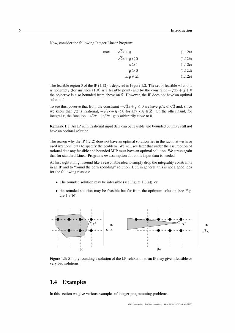
Example 1.2Consider the following Integer Linear Program:

max x+y (1.9a)

2y−3x! 2 (1.9b)

x+y! 5 (1.9c)

1 ! x! 3 (1.9d)

1 ! y! 3 (1.9e)

x,y ∈Z (1.9f)

The feasible region S of the problem is depicted in Figure 1.1. It consists of the integralpoints emphasized in red, namely

S= {(1,1),(2,1),(3,1),(1,2),(2,2),(3,2),(2,3)}.

▹

File: –sourcefile– Revision: –revision– Date: 2015/10/27 –time–GMT

4 Introduction

0 1 2 3 4 5

0

1

2

3

4

5

Figure 1.1: Example of the feasible region of an integer program.

Example 1.3 (Knapsack Problem)A climber is preparing for an expedition to Mount Optimization. His equipment consistsof n items, where each item i has a profit pi ∈ Z+ and a weight wi ∈ Z+. The climberknows that he will be able to carry items of total weight at most b ∈Z+. He would like topack his knapsack in such a way that he gets the largest possible profit without exceedingthe weight limit.

We can formulate the KNAPSACK problem as a (BIP). Define a decision variable xi, i =1, . . . ,n with the following meaning:

xi =

!

1 if item i gets packed into the knapsack0 otherwise

Then, KNAPSACK becomes the (BIP)

maxn"

i=1

pixi (1.10a)

n"

i=1

wixi ! b (1.10b)

x ∈ Bn (1.10c)

▹

In the preceeding example we have essentially identified a subset of the possible items witha 0-1-vector. Given a ground set E, we can associate with each subset F ⊆ E an incidence

vector χF ∈RF by setting

χFe =

!

1 if e ∈ F

0 if e /∈ F.

Then, we can identify the vector χF with the set F and vice versa. We will see numerousexamples of this identification in the rest of these lecture notes. This identification appearsfrequently in the context of combinatorial optimization problems.

File: –sourcefile– Revision: –revision– Date: 2015/10/27 –time–GMT

1.3 Notes of Caution 5

Definition 1.4 (Combinatorial Optimization Problem)A combinatorial optimization problem is given by a finite ground set N, a weight function

c : N→R and a family F ⊆ 2N of feasible subsets of N. The goal is to solve

(COP) min

⎧⎨

⎩

∑

j∈S

cj : S ∈ F

⎫⎬

⎭. (1.11)

Thus, we can write KNAPSACK also as (COP) by using:

N := {1, . . . ,n}

F :=

{

S⊆N :∑

i∈S

wi ! b

}

,

and c(i) := −wi. We will see later that there is a close connection between combinatorialoptimization problems (as stated in (1.11)) and Integer Linear Programs.

1.3 Notes of Caution

Integer Linear Programs are qualitatively different from Linear Programs in a number ofaspects. Recall that from the Fundamental Theorem of Linear Programming we know that,if the Linear Program (1.1) is feasible and bounded, it has an optimal solution.

0 1 2 3 4 5 6 7 8

0

1

2

3

4

5

6

7

8y=√

2xx= 1

y= 0

Figure 1.2: An IP without optimal solution.

File: –sourcefile– Revision: –revision– Date: 2015/10/27 –time–GMT

6 Introduction

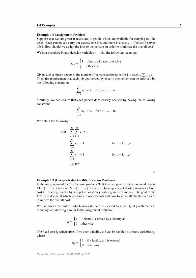
Now, consider the following Integer Linear Program:

max −√

2x+y (1.12a)

−√

2x+y! 0 (1.12b)

x" 1 (1.12c)

y" 0 (1.12d)

x,y ∈Z (1.12e)

The feasible region S of the IP (1.12) is depicted in Figure 1.2. The set of feasible solutionsis nonempty (for instance (1,0) is a feasible point) and by the constraint −

√2x+y ! 0

the objective is also bounded from above on S. However, the IP does not have an optimalsolution!

To see this, observe that from the constraint −√

2x+y! 0 we have y/x!√

2 and, sincewe know that

√2 is irrational, −

√2x+y < 0 for any x,y ∈ Z. On the other hand, for

integral x, the function −√

2x+ ⌊√

2x⌋ gets arbitrarily close to 0.

Remark 1.5 An IP with irrational input data can be feasible and bounded but may still nothave an optimal solution.

The reason why the IP (1.12) does not have an optimal solution lies in the fact that we haveused irrational data to specify the problem. We will see later that under the assumption ofrational data any feasible and bounded MIP must have an optimal solution. We stress againthat for standard Linear Programs no assumption about the input data is needed.

At first sight it might sound like a reasonable idea to simply drop the integrality constraintsin an IP and to “round the corresponding” solution. But, in general, this is not a good ideafor the following reasons:

• The rounded solution may be infeasible (see Figure 1.3(a)), or

• the rounded solution may be feasible but far from the optimum solution (see Fig-ure 1.3(b)).

x∗

cTx

(a)

x∗

cTx

(b)

Figure 1.3: Simply rounding a solution of the LP-relaxation to an IP may give infeasible orvery bad solutions.

1.4 Examples

In this section we give various examples of integer programming problems.

File: –sourcefile– Revision: –revision– Date: 2015/10/27 –time–GMT

1.4 Examples 7

Example 1.6 (Assignment Problem)Suppose that we are given n tasks and n people which are available for carrying out thetasks. Each person can carry out exactly one job, and there is a cost cij if person i servesjob j. How should we assign the jobs to the persons in order to minimize the overall cost?

We first introduce binary decision variables xij with the following meaning:

xij =

!

1 if person i carrys out job j

0 otherwise.

Given such a binary vector x, the number of persons assigned to job j is exactly"n

i=1 xij.Thus, the requirement that each job gets served by exactly one person can be enforced bythe following constraint:

n#

i=1

xij = 1, for j= 1, . . . ,n.

Similarly, we can ensure that each person does exactly one job by having the followingconstraint:

n#

j=1

xij = 1, for i= 1, . . . ,n.

We obtain the following BIP:

minn#

i=1

n#

j=1

cijxij

n#

i=1

xij = 1 for j= 1, . . . ,n

n#

j=1

xij = 1 for i= 1, . . . ,n

x ∈ Bn2

▹

Example 1.7 (Uncapacitated Facility Location Problem)In the uncapacitated facility location problem (UFL) we are given a set of potential depotsM= {1, . . . ,m} and a set N= {1, . . . ,n} of clients. Opening a depot at site j involves a fixedcost fj. Serving client i by a depot at location j costs cij units of money. The goal of theUFL is to decide at which positions to open depots and how to serve all clients such as tominimize the overall cost.

We can model the cost cij which arises if client i is served by a facility at j with the helpof binary variables xij similar to the assignment problem:

xij =

!

1 if client i is served by a facility at j0 otherwise.

The fixed cost fj which arises if we open a facility at j can be handled by binary variables yj

where

yj =

!

1 if a facility at j is opened0 otherwise.

File: –sourcefile– Revision: –revision– Date: 2015/10/27 –time–GMT

8 Introduction

Following the ideas of the assignment problem, we obtain the following BIP:

minm!

j=1

fjyj+

m!

j=1

n!

i=1

cijxij (1.13a)

m!

j=1

xij = 1 for i= 1, . . . ,n (1.13b)

x ∈ Bnm,y ∈ Bm (1.13c)

As in the assignment problem, constraint (1.13b) enforces that each client is served. Butour formulation is not complete yet! The current constraints allow a client i to be servedby a facility at j which is not opened, that is, where yj = 0. How can we ensure that clientsare only served by open facilities?

One option is to add the nm constraints xij ! yj for all i, j to (1.13). Then, if yj = 0, wemust have xij = 0 for all i. This is what we want. Hence, the UFL can be formulated asfollows:

minm!

j=1

fjyj+

m!

j=1

n!

i=1

cijxij (1.14a)

m!

j=1

xij = 1 for i= 1, . . . ,n (1.14b)

xij ! yj for i= 1, . . . ,n and j= 1, . . . ,m (1.14c)

x ∈ Bnm,y ∈ Bm (1.14d)

A potential drawback of the formulation (1.14) is that it contains a large number of con-straints. We can formulate the condition that clients are served only by open facilities inanother way. Observe that

"ni=1 xij is the number of clients assigned to facility j. Since

this number is an integer between 0 and n, the condition"n

i=1 xij ! nyj can also be usedto prohibit clients being served by a facility which is not open. If yj = 0, then

"ni=1 xij

must also be zero. If yj = 1, we have the constraint"n

i=1 xij !n which is always satisfiedsince there is a total of n clients. This gives us the alternative formulation of the UFL:

minm!

j=1

fjyj+

m!

j=1

n!

i=1

cijxij (1.15a)

m!

j=1

xij = 1 for i= 1, . . . ,n (1.15b)

n!

i=1

xij ! nyj for j= 1, . . . ,m (1.15c)

x ∈ Bnm,y ∈ Bm (1.15d)

Are there any differences between the two formulations as far as solvability is concerned?We will explore this question later in greater detail. ▹

Example 1.8 (Minimum Spanning Tree Problem)A spanning tree in an undirected graph G = (V ,E) is a subgraph T = (V ,F) of G whichis connected and does not contain cycles. Given a cost function c : E→ R+ on the edgesof G the minimum spanning tree problem (MST-Problem) asks to find a spanning tree T ofminimum weight c(F).

File: –sourcefile– Revision: –revision– Date: 2015/10/27 –time–GMT

1.4 Examples 9

We choose binary indicator variables xe for the edges in E with the meaning that xe = 1if and only if e is included in the spanning tree. The objective function

!

e∈E cexe isnow clear. But how can we formulate the requirement that the set of edges chosen forms aspanning tree?

A cut in an undirected graph G is a partition S∪ S̄ = V , S∩ S̄ = ∅ of the vertex set. Wedenote by δ(S) the set of edges in the cut, that is, the set of edges which have exactly oneendpoint in S. It is easy to see that a subset F⊆ E of the edges forms a connected spanningsubgraph (V ,F) if and only if F∩ δ(S) ̸= ∅ for all subsets S with ∅ ⊂ S ⊂ V . Hence, wecan formulate the requirement that the subset of edges chosen forms a connected spanningsubgraph by having the constraint

!

e∈δ(S) xe ! 1 for each such subset. This gives thefollowing BIP:

min"

e∈E

cexe (1.16a)

"

e∈δ(S)

xe ! 1 for all ∅⊂ S⊂ V (1.16b)

"

e∈E

xe = n−1 (1.16c)

x ∈ BE (1.16d)

The constraint!

e∈E xe = n− 1 ensures that our subgraph contains exactly n− 1 edges,which together with the requirement that it is connected, implies that it forms a spanningtree.

▹

Example 1.9 (Traveling Salesman Problem)In the traveling salesman problem (TSP) a salesman must visit each of n given cities V ={1, . . . ,n} exactly once and then return to his starting point. The distance between city iand j is cij. The salesman wants to find a tour of minimum length.

The TSP can be modeled as a graph problem by considering a complete directed graph G=(V ,A), that is, a graph with A = V×V , and assigning a cost c(i, j) to every arc a = (i, j).A tour is then a cycle in G which touches every node in V exactly once.

We formulate the TSP as a BIP. We have binary variables xij with the following meaning:

xij =

#

1 if the salesman goes from city i directly to city j

0 otherwise.

Then, the total length of the tour taken by the salesman is!

i,j cijxij. In a feasible tour,the salesman enters each city exactly once and also leaves each city exactly once. Thus, wehave the constraints:

"

j:j̸=i

xji = 1 for i= 1, . . . ,n

"

j:j̸=i

xij = 1 for i= 1, . . . ,n.

However, the constraints specified so far do not ensure that a binary solution forms indeeda tour.

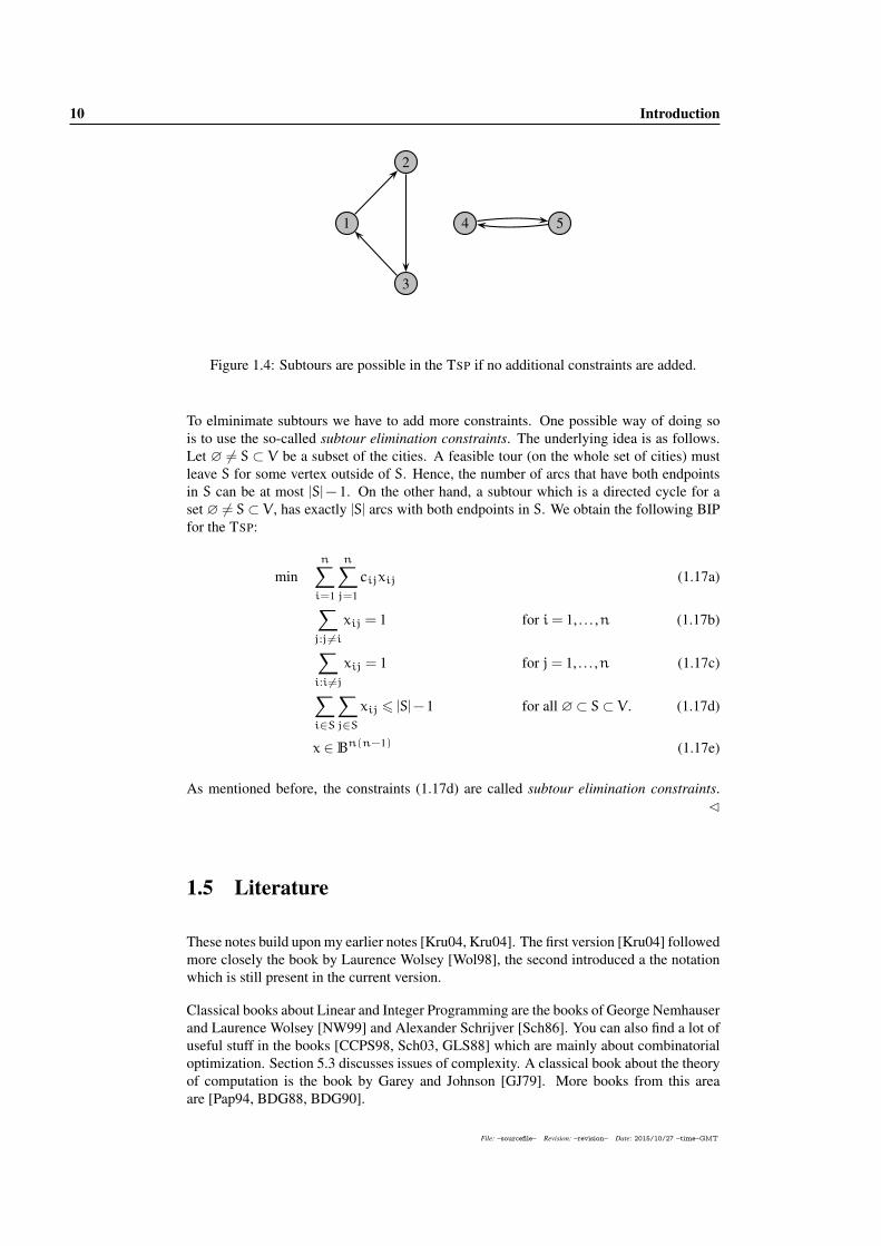
Consider the situation depicted in Figure 1.4. We are given five cities and for each citythere is exactly one incoming and one outgoing arc. However, the solution is not a tour buta collection of directed cycles called subtours.

File: –sourcefile– Revision: –revision– Date: 2015/10/27 –time–GMT

10 Introduction

2

1 4 5

3

Figure 1.4: Subtours are possible in the TSP if no additional constraints are added.

To elminimate subtours we have to add more constraints. One possible way of doing sois to use the so-called subtour elimination constraints. The underlying idea is as follows.Let ∅ ̸= S ⊂ V be a subset of the cities. A feasible tour (on the whole set of cities) mustleave S for some vertex outside of S. Hence, the number of arcs that have both endpointsin S can be at most |S|− 1. On the other hand, a subtour which is a directed cycle for aset ∅ ̸= S⊂ V , has exactly |S| arcs with both endpoints in S. We obtain the following BIPfor the TSP:

minn!

i=1

n!

j=1

cijxij (1.17a)

!

j:j̸=i

xij = 1 for i= 1, . . . ,n (1.17b)

!

i:i̸=j

xij = 1 for j= 1, . . . ,n (1.17c)

!

i∈S

!

j∈S

xij ! |S|−1 for all ∅⊂ S⊂ V . (1.17d)

x ∈ Bn(n−1) (1.17e)

As mentioned before, the constraints (1.17d) are called subtour elimination constraints.▹

1.5 Literature

These notes build upon my earlier notes [Kru04, Kru04]. The first version [Kru04] followedmore closely the book by Laurence Wolsey [Wol98], the second introduced a the notationwhich is still present in the current version.

Classical books about Linear and Integer Programming are the books of George Nemhauserand Laurence Wolsey [NW99] and Alexander Schrijver [Sch86]. You can also find a lot ofuseful stuff in the books [CCPS98, Sch03, GLS88] which are mainly about combinatorialoptimization. Section 5.3 discusses issues of complexity. A classical book about the theoryof computation is the book by Garey and Johnson [GJ79]. More books from this areaare [Pap94, BDG88, BDG90].

File: –sourcefile– Revision: –revision– Date: 2015/10/27 –time–GMT

1.6 Acknowledgements 11

1.6 Acknowledgements

I wish to thank all students of the lecture »Optimization II: Integer Programming« at theTechnical University of Kaiserslautern (winter semester 2003/04) for their comments andquestions. Particular thanks go to all students who actively reported typos and providedconstructive criticism: Robert Dorbritz, Ulrich Dürholz, Tatjana Kowalew, Erika Lind,Wiredu Sampson and Phillip Süß. Needless to say, all remaining errors and typos aresolely my faults!

File: –sourcefile– Revision: –revision– Date: 2015/10/27 –time–GMT