Integrability of the AdS 5 ×S 5 Superstring in Uniform Light-Cone Gauge Diplomarbeit zur Erlangung des akademischen Grades des Diplom Physikers (Dipl. Phys.) Humboldt-Universit¨ at zu Berlin Mathematisch-Naturwissenschaftliche Fakult¨ at I Institut f¨ ur Physik Lehrstuhl f¨ ur Quantenfeldtheorie und Stringtheorie eingereicht von Alexander Hentschel geboren 3. August 1980 in Rostock, Deutschland Gutachter: Prof. Dr. Jan Plefka Prof. Dr. Ulrich Wolff Berlin, 31. Juli 2007
Transcript
Integrability of the AdS5×S5 Superstring in Uniform
Light-Cone Gauge
Diplomarbeitzur Erlangung des akademischen Grades
des Diplom Physikers (Dipl. Phys.)
Humboldt-Universitat zu BerlinMathematisch-Naturwissenschaftliche Fakultat I
Institut fur PhysikLehrstuhl fur Quantenfeldtheorie und Stringtheorie
eingereicht von Alexander Hentschelgeboren 3. August 1980in Rostock, Deutschland
Gutachter: Prof. Dr. Jan PlefkaProf. Dr. Ulrich Wolff
Berlin, 31. Juli 2007
Hilfsmittel
Diese Diplomarbeit wurde mit LATEX und BibTEX gesetzt. Die Grafiken wurden mit Ma-cromedia Freehand 10 erstellt. Die in dieser Arbeit enthaltenen Rechnungen wurden unterEinbeziehung von Jos Vermaserens Form 3.1, Wolfram Research Mathematica 5.2 und GNUgcc 3.3.5 erstellt.
Selbstandigkeitserklarung
Hiermit erklare ich, die vorliegende Diplomarbeit selbstandig sowie ohne unerlaubte fremdeHilfe verfasst und nur die angegebenen Quellen und Hilfsmittel verwendet zu haben.
Mit der Auslage meiner Diplomarbeit in den Bibliotheken der Humboldt Universitat zu Berlinbin ich einverstanden.
Berlin, 31. Juli 2007 Alexander Hentschel
Acknowledgements
First of all, at this opportunity I would like to thank my mother Cornelia Hentschel for alwayshaving supported me throughout my life, unremittingly assisting me with her experience of lifeand helping me keeping up my studies. She has a great stake in the success of my work.
From the Quantum Field Theory and String Theory Group of the Humboldt-Universityof Berlin I wish to devote many thanks to my supervisor Prof. Jan Plefka for his excellentsupervision, encouragement and patience as well as supporting my future life in many cases. Iwould also like to thank Prof. Ulrich Wolff for appraising this diploma thesis even though stringtheory is not his specific field of research. For many illuminating discussions, dedicating plentyof time for this work as well as for his friendship I thank Per Sundin. I enjoyed very muchworking in the QFT and String Theory Group and would like to thank all group membersfor the friendly, communicative and personal atmosphere, especially Silvia Richter for heradministrative assistance and her dedication for social concerns and Dr. Hans-Jorg Otto formaintaining our computers.
I would like to express my gratitude and appreciation to Prof. Dietmar Ebert for beingdevotedly active in teaching and reminding students to keep in mind regarding the overallpicture and developments in physics, life and society. Prof. Ebert has continuously supportedme as a mentor for many years with personal and well-considered advice. In this respect I amalso especially thankfull to Dr. Alejandro Saenz for dedicating plenty of time in supporting myfuture life with advice and assistance.
I would like to devote special thanks to my colleague Andreas Rodigast for many hoursof discussions and help. Finally I would like to thank my colleagues Max Dohse, Jens Grieger,Volker Branding, Nicolai Beck, Hai Ngo Than, Ralf Sattler and Johannes Vetter for the friendlyand personal atmosphere and the many discussions, some about physical and lots about othertopics in life.
Warm thanks are also devoted to my best friend Felix Hermann who is sedulously assi-sting me with advice and his support in all possible situations of live. Last but certainly notleast I would thank Anke Schneider for her moral support, understanding and for being alwaysa good friend to me.
Inhaltsangabe
In der vorliegenden Diplomarbeit wird im nahen Plane-wave Limes ein detaillierter Test derQuantenintegrabilitat des AdS5 × S5−Superstrings in uniformer Lichtkegeleichung durchge-fuhrt. Einleitend wird die perturbative Herleitung des Superstringhamiltonians zusammenge-fasst. Auf dieser Grundlage wird eine Methode zur systematischen Berechnung des Energie-spektrums einer allgemeinen Stringkonfiguration entwickelt, die ich in der sogenannten Abakus-Software implementiert habe.Der zweite Teil der Diplomarbeit behandelt den Betheansatz und die Ableitung der psu(2, 2|4)Bethegleichungen. Die Losungen dieser Gleichungen liefern die Skalendimensionen eichinva-rianter zusammengesetzter Operatoren der N = 4 Super-Yang-Mills-Theorie, die gemaß derAdS/CFT-Korrespondenz dem Stringenergiespektrum entsprechen.Die durch Diagonalisierung des Lichtkegelhamiltonians berechneten Energiespektren werdenmit den Losungen der Bethegleichungen verglichen, wobei die Untersuchung sowohl analyti-sche als auch numerische Ergebnisse von Zustanden mit maximal sechs Anregungen umfasst. Inallen untersuchten Fallen wurde exakte Ubereinstimmung der Spektren gefunden, was die ver-mutete Eigenschaft der Quantenintegrabilitat des AdS5× S5−Superstrings stark untermauert.
Abstract
In the present diploma thesis a detailed test of the quantum integrability of the AdS5× S5 su-perstring in uniform light cone-gauge is performed in the near plane-wave limit. Preliminarythe perturbative derivation of the superstring Hamiltonian in AdS5 × S5 is reviewed. Basedthereon a method is developed to systematically compute the energy spectrum of generic stringconfigurations, which I have implemented in a software system called Abakus.In the second part the Bethe ansatz is introduced and the derivation of the psu(2, 2|4) Betheequations is reviewed, yielding the scaling dimension of composite gauge invariant operatorsof N = 4 super Yang-Mills theory, which is according to the AdS/CFT correspondence equalto the string energy spectrum.The energy spectra obtained by diagonalization of the light-cone Hamiltonian are thereuponconfronted with the solutions of the Bethe equations. The analysis is performed both analyti-cally and numerically up to the level of six impurity states, where perfect agreement is foundlending strong support to the quantum integrability of the AdS5 × S5 superstring.
Contents
Contents
1 Introduction 5
2 AdS/CFT correspondence and integrability 72.1 Integrability in Gauge Theory and String Theory . . . . . . . . . . . . . . . . . 9
In nature one observes four fundamental forces, which are strong, weak and electromagneticinteraction as well as gravity. At energy scales accessible nowadays the first three interactionsare preeminently described by quantum field theories and are combined to a uniform theory bythe Standard Model of particle physics. All quantum field theories of the Standard Model aregauge field theories, wherein spin-1 particles are responsible for transmitting the interaction.Gauge theories contain more degrees of freedom than the original physical system. The gaugetransformations relate physically equivalent field configurations and form a group. In contrastto the gauge group U(1) of quantum electrodynamics, the gauge group SU(3) of quantumchromodynamics (QCD) and SU(2) of weak interaction are non-Abelian. This property reflectsthe fact that the gauge particles are self-interacting. At energy scales accessible nowadays theelectroweak coupling is small so perturbation theory is applicable. In QCD the situation isquite different: at low energy the coupling constant for the interaction is large, which leadsto confinement, while it is small for high energies, resulting in asymptotic freedom of quarks.In the latter perturbation theoretical methods are not applicable, since a power series in thecoupling constant does not converge. So far quantum field theories work well in the regime ofsmall couplings, while the strong coupling behavior is understood less well, accessible todayonly via numerical computations on a discretized spacetime lattice.
For the remaining force of gravity there is currently only a classical theory available,which is the theory of General Relativity. It works well at large length scales corresponding tolow energies. Yet a microscopical description of spacetime at lengths near the Planck scale orenergies near the Planck energy requires a quantum theory of gravity. The attempt to quantizegravity according to the known procedures leads to a non-renormalizable field theory. Despitenon-renormalizability it is nevertheless useful as an effective quantum theory [1] in the lowenergy limit, including the massless spin-2 graviton as exchange particle of gravitation. But afully consistent theory of quantum gravity has still not been constructed.Also a unified quantum theory of gravitation and the Standard Model is needed to describephysics in highly curved backgrounds, like near the horizons of black holes. In such an envi-ronment one needs a generalization of the Standard Model including a microscopic theory ofgravity. One of the most promising candidates for such a theory is string theory. While inthe Standard Model elementary particles are considered to be pointlike and to interact locally,string theory drops this notion and assumes that the fundamental objects are one-dimensionalstrings.
Even though the motivation for string theory given nowadays is quite different, it wasoriginally developed in an attempt to describe the large number of mesons and hadrons thatwere experimentally discovered. One surprising issue of the hadronic spectrum is, the hadronscan be sorted into groups in such way that, within every group, mass m and Spin J obey arelation like m2 ∼ α0 + TJ , where only the intercept α0 differs for each group. This prop-erty is well explained by assuming the particles to be different oscillation modes of a rotating,relativistic string with tension T . Unfortunately string theory in this context leads to someproperties which drastically disagree with experimental findings. Due to the use of extendedobjects, string theory predicts an exponential falloff of scattering amplitudes but only pow-erlike behaviors (possibly deformed by structure functions) have been observed. Later it wasdiscovered that hadrons and mesons are actually built of quarks and the appropriate theoreti-cal description is a non-Abelian SU(3) gauge field theory.But replacing the picture of pointlike particles by using one-dimensional extended objects ofa very small size is actually a quite natural generalization, because by viewing the system onmuch larger scales, the strings reduce to an almost pointlike structure and therefore string
5
theory is expected to reproduce many features of conventional gauge theories on larger scales.To the best of our knowledge the only consistent interaction for massless spin-2 particles isthat of gravity and since all string theories include such a particle, which is identified with thedesired graviton, string theories could represent a unified description of quantized gravity aswell as quantum field theories.One fascinating aspect of string theory is that quantum consistency demands that the theoryoccupies ten spacetime dimensions1. However, we observe only four spacetime dimensions, sotheorists are charged with the task of understanding the role of the six extra spatial dimen-sions, but since it is not known how spacetime looks like at short distances comparable toPlanck length, the extra dimensions could simply be highly curved and thus so tiny that it isimpossible to detect them at energy scales accessible today.
The course of studying gauge theories and string theories has led to the discovery of adramatically new class of fundamental symmetries known as dualities. These symmetries standapart from traditional ones in the sense that dualities connect physical theories which, at leastsuperficially, appear to be entirely distinct in their formulation. In particular two seeminglydifferent theories are considered to be dual, if both models describe equivalent physical sys-tems.A well known example is T-duality: type IIA string theory with one spatial dimension compact-ified on a circle of radius R can be translated to type IIB string theory with compactificationradius R−1. The usefulness of duality derives in part from the fact that dual descriptions aretypically complementary, insofar as information that is inaccessible in one physical theory mayoften be extracted from a straightforward calculation in the theory’s dual description.
In this work we will primarily be concerned with an other famous duality, which is theso called AdS/CFT correspondence. One specific property of the AdS/CFT correspondenceis that it claims a strongly coupled super Yang-Mills theory to be dual to a weakly coupledstring theory. Provided this duality holds, string theory allows us to access the non-pertubativeregime of strongly interacting non-Abelian gauge theories without being restricted to numericalcomputations on a discrete space-time lattice. It is therefore promising to study string theory,irrespective of whether it will succeed to provide a unified quantum theory of all fundamentalforces.Another very important question to address is, how string theory behaves in a highly curvedbackground, where the extension of single strings is of magnitude of the curvature radius ofspacetime. In respect thereof very little is known, since perturbative string theory is notapplicable anymore. But using the AdS/CFT correspondence the other way around it givesrise to this regime by working in the dual weakly coupled super Yang-Mills theory.
Altogether the AdS/CFT correspondence could provides us with a powerful tool to ex-plore previously almost unaccessible regimes of different theories. Even though AdS/CFTcorrespondence has passed several nontrivial test it has not been proven yet.
1 M-theory is provided with an extra 11th dimension. By different compactifications of this extra dimensionM-theory can be reduced to every type of 10-dimensional string theory.
6
Chapter 2: AdS/CFT correspondence and integrability
2 AdS/CFT correspondence and integrability
The duality of compactifications of M/sting theory on various Anti-deSitter (AdS) space-times and various conformal field theories was conjectured by Maldacena 1998 [2], known asAdS/CFT correspondence. Maldacena’s conjecture is based on an idea by ’t Hooft [3]: startingwith an SU(N) Yang-Mills theory with coupling gY M and N colours one can classify Feyn-mann graphs according to the their genus H, i.e. the minimum number of handles that mustbe added to a plane to embed the graph without any crossings of lines. The crucial fact ob-served by ’t Hooft is, that each Feynmann diagram is associated with a factor r = λlN2−2H−L,depending on its number of loops l and genus H. The quantity L enumerates the number offermionic loops2 and the ’t Hooft coupling is defined as λ = g2
Y MN . In the ’t Hooft limitN →∞, gY M → 0 with λ fixed, the free energy F of SU(N) gauge theory takes the pictorialform:
F = N2 + 1 +1N2
+ . . . = N2∞∑
H=0
1N2H
∞∑l=0
cg,l λl (2.1)
Obviously this genus expansion resembles the pertubative expansion of a string theory in thestring couplin constant gs ∝ N−1. For large N the string theory becomes free and thus onlyplanar diagramms contribute in the corresponding gauge theory.
The presented argument suggests that different kinds of gauge theories will correspondto differents sting theories but according to experience it is extremely difficult to prove suchequivalences. In its purest form, the conjectured AdS/CFT correspondece identifies the typeIIB supersting in a ten dimensional anti-de-Sitter cross sphere (AdS5×S5) background withthe maximally supersymmetric Yang-Mills theory3 with gauge group SU(N) and N = 4 spinorsupercharges in four dimensions (N = 4 SYM). The gauge theory’s Langrangian is completelydetermined by supersymmetry which has a global SU(4)R R-symmetry that rotates the sixscalar fields and four fermions. Furthermore it is invariant with respect to the conformal groupSO(4, 2) in four dimensions, including the usual Poincare transformations as well as scaletransformations and special conformal transformations.These symmetries have to be reflected by the dual string theory description. In fact the fivedimensional Anti-de-Sitter space is the only space with local SO(4, 2) isometry. It is themaximally symmetric solution of Einstein’s euations with negative cosmological constant. Atthe border of the AdS5 the remaining five dimensions of the 10 dimensional target space, thetype IIB superstring is moving in, are compactified on a five sphere S5. Thus the SU(4)symmetry of the SYM theory is reproduced by the locally isomorphic SO(6) symmetry of S5
on the string side.To establish a connection between the two theories, one has to relate the free parameters
of the different models to each other. N = 4 SYM theory is controlled by the rank N of thegauge group and the coupling constant gY M or eqivalently λ = g2
Y MN while string theory isparemetrized by the effective string tension R2/α′ and the string coupling gs, where R is thecommon radius of the AdS5 and S5 geometries and 1/α′ denotes the string tension. Accordingto the AdS/CFT proposal, these two sets of parameters are identified as
gs =4πλN
,√λ =
R2
α′. (2.2)
2 In an SU(N) gauge theory there are fermionic particles and gauge bosons transmitting the interaction. Touse a uniform notation for differen values of N , we denote the fermions as “quarks” and the SU(N) charge as“colour” (in this convention we also refer to the weak isospin as SU(2) colour). In this notation l is associatedwith the number of closed colour loops, while L counts only closed quark loops.
3 Due to it’s vanishing β-function, N = 4 SYM is a conformal field theory (CFT).
7
Low-energy gravitational description in terms of classical type IIB supergravity is perturba-tively valid in weakly curved geometries (compared to string units), i.e. for
√λ 1, while
perturbative field theory is applicable only in the domain of gY M 1, viz small λ. Hence oneis facing a strong/weak coupling duality, as stated in chapter 1.
By the physical equivalence of both theories it is required, that for each field O(x) onthe boundary Minkowski theory there is a field φ(x, z) in the bulk string theory with theproperty that at least the corresponding correlators of both theories agree on the boundary.It is conjectured that the partition function of string theory on AdS5×S5 coincides with thegenerating function of N = 4 super Yang-Mills on the boundary of AdS5×S5 [4]:
〈e∫d4x φ0(~x) O(~x)〉CFT = ZString
[φ0(~x, z)
∣∣z=0
](2.3)
where the left hand side is the generating function of correlation functions in the field theory,i.e. φ0 is an arbitrary function and we can calculate correlation functions of O by takingfunctional derivatives with respect to φ0 and than setting φ0 = 0. The right hand side denotesthe full partition function of string theory with the boundary condition that the field φ(x, z)has the value φ(x, z)
∣∣z=0
= φ0(x) on the boundary of AdS. Thus each field propagating on AdSspace is in a one-to-one correspondence with an operator of SYM. For the D = 10 supergravitymultiplet the explicit mapping is given in [5].
Based on (2.3), the energy eigenvalue E of a string state |φA〉 has been identified with thescaling dimension ∆ of the dual gauge theory operator OA(x) [4], which in turn is determinedfrom the two point function of the conformal field theory by
〈OA(x)OB(y)〉 =δ∆
OA,∆
OB
(x− y)2∆OA
. (2.4)
The O denote composite gauge invariant operators of the form O(x) = Tr(φi1(x) . . . φin(x)),where the φj are elementary fields of N = 4 SYM and their covariant derivatives in the adjointrepresentation of SU(N).This remarkable result
∆(λ,1N
) ≡ E(R2
α′, gs) (2.5)
allows for determination of the all loop scaling dimension in planar gauge theory by calculatingthe Energy in free string theory in the large N limit. Nevertheless string quantization anddetermination of its quantum spectrum in curved backgrounds, even in the highly symmetricAdS5×S5 space, remains unknown. 2002 Berenstein, Maldacena and Nastase considered anovel limit of a degenerated pointlike string configuration, corresponding to a particle rotatingwith large angular momentum J on a great circle of the S5 space [6]. In this so called ‘BMNlimit’ of J →∞ with λ/J2 fix, from the fastly moving particles point of view, the geometry ofAdS5×S5 limits to a gravitational plane wave background
In ‘uniform light-cone gauge’ an exact world-sheet Hamiltonian has been established in[7] and pertubatively quantized in the near-plane wave limit using J → ∞. We are going toreview this derivation in section 3. Thus the spectrum of total arbitrary string states can inprinciple be computed in order 1/J and this in turn leads to various predictions for the anomalscaling dimensions of corresponding gauge theory operators.
8
Chapter 2: AdS/CFT correspondence and integrability
2.1 Integrability in Gauge Theory and String Theory
In testing the conjectured AdS/CFT correspondece very important progress has been madeduring recent years building on the concept on integrability [8]. In classical mechanics there isa well-known definition of integrability due to Liouville: a finite-dimensional system is calledintegrable if it possesses a set of independently conserved charges Qi commuting with respectto the Poisson bracket
Qi,Qj
= 0
and the total number of conserved charges including the Hamiltonian is half of the dimensionof the phase space. For quantum theories there is no such strict definition of integrabilityknown, however, it is expected that a quantum system is integrable if the number of conservedcharges equals the number of degrees of freedom in the system.From the most pragmatical point of view one might call a system quantum integrable [9] ifprovides the opportunity to “exactly” determine the quantities of physical interest. In thegiven context “exact” means that one can state a fixed set of equations which determine thesequantities exactly, however, about the solvability of these equations one does not care at thispoint.
It has emerged that in planar gauge theory the dilaton operator, whose spectrum yieldsthe desired scaling dimension of composite, gauge invariant operators, is isomorphic to theHamiltonian of an integrable quantum spin chain [10],[11]. The property of integrability guar-antees the existence of a Bethe ansatz which in principle allows for reformulating the quantumspectral problem into the solution of a set of non-linear algebraic equations, the Bethe equa-tions. In other words, the Bethe equations diagonalize the planar gauge theory dilatationoperator in the sense that its solutions, the Bethe roots, are eigenvalues of the dilatationoperator.
With the AdS/CFT conjecture in mind, immediately a question arises: is the type IIBsuperstring, propagating in AdS5×S5, a quantum integrable model and is its energy spectrumindeed described by this set of Bethe equations?Addressing these questions is important, since it will lead to a highly nontrivial test of theAdS/CFT duality conjecture. Moreover the Bethe equations are all -loop equations4 and there-fore yield all loop predictions of the quantum string spectrum or the dual scaling dimension ofcomposite, gauge invariant operators, if we manage to solve them non-perturbatively.
In order to investigate the integrability of the AdS5 × S5 superstring the perturbative deriva-tion the Hamiltonian is reviewed in section 3. Based thereon in chapter 4 a computer algebraicmethod is described, which makes it possible to systematically compute the energy spectrum ofgeneric string configurations. In section 5 the superstring spectra are derived analytically andnumerically in all closed subsectors for up to six string excitations. Since the light-cone energyis only determined implicitly by the derived string spectra of section 5 the explicit solution forthe energy is presented in chapter 6.The Bethe ansatz leading to psu(2, 2|4) Bethe equations is reviewed in chapter 7 followed by adetailed discussion in section 8 how to solve these equations in the various sectors. The resultsare compared to the string results obtaied in section 4.
4 For a spin chain of length L, by construction [12] the Bethe equations are exact only up to order ` < L withrespect to the expansion in g ∼
√λ 1 for gauge theory and 1/J 1 in string theory. Consequently the
Bethe roots yield all-loop predictions only in the case of an infinite long chain.
9
10
Chapter 3: The Superstring on AdS5 × S5
3 The Superstring on AdS5 × S5
This section will start with some general remarks on the AdS5×S5 space. The derivation of thestring Hamiltonian is exemplified for the bosonic case in paragraph 3.2 followed by a discussionof the full Hamiltonian including fermions. Subsequently a notation for generic string states isintroduced and some general remarks on the Hamiltonian eigenvalues are presented. Section3 is concluded with the derivation of the spectrum for a generic su(2) string states.
3.1 The AdS5 × S5 space
Embedding the five-dimensional anti-de-Sitter space and the five sphere in R6 the S5 is de-scribed by s21 + s22 + . . .+ s26 = R and AdS5 by −a2
−1−a20 +a2
1 +a22 + . . .+a2
4 = −R. R denotesthe common radius of AdS5 and S5. By parametrization through
s1 + i s2 = sin ξ cosψ ei φ1 , s3 + i s4 = sin ξ sinψ ei φ2 , s5 + i s6 = cos ξ ei φ ,a1 + i a2 = sinh ρ cos ψ ei ϕ1 , a3 + i a4 = sinh ρ sin ψ ei ϕ2 , a−1 + i a0 = cosh ρ ei t
Performing a suitable reparametrization t, ρ, ψ, ϕ1, ϕ2 → t, z1, . . . , z4, φ, ξ, ψ, φ1, φ2 →φ, y1, . . . , y4 of the form
cosh ρ =(1 + z2/4)(1− z2/4)
, cos ξ =(1− y2/4)(1 + y2/4)
with z2 = zkzk, y2 = ykyk, k = 1, . . . , 4
one can cast the metric for the AdS5 × S5 product space into
ds2AdS5×S5 = −
(1 + z2/41− z2/4
)2
dt2 +dzkdzk
(1− z2/4)2︸ ︷︷ ︸metric of AdS5
+(
1− y2/41 + y2/4
)2
dφ2 +dykdyk
(1 + y2/4)2︸ ︷︷ ︸metric of S5
. (3.2)
By construction, the AdS5×S5 space has the symmetry SO(2, 4)×SO(6), but only translationinvariance in t and φ and the SO(4)×SO(4) symmetry of the coordiantes zk, yk remain manifestin this form.
• Introduction to AdS5 × S5: picture, time winding, Metric
For the sake of simplicity the following notations are used in the next chaptert =: z0 time on AdS5 t, za ≡ zµ, a = 1, ..., 4, µ = 0, ..., 4 coordinates on AdS5
φ =: y0 angle on S5 t, ys ≡ yν , s = 1, ..., 4, ν = 0, ..., 4 coordinates on S5
xM ≡ za, ys, a, s = 1, ..., 4 remaining coordinates on AdS5 × S5 excluding t, φ
3.2 The bosonic Superstring on AdS5 × S5
In this chapter the bosonic part of the superstring Hamiltonian will be derived in order todemonstrate the basic procedure to quantize the AdS5 × S5 Superstring perturbatively. Westart with the well known Polyakov action where the fermionic contribution is omitted
I =∫dτdσ L with L = −
√λ
4πγαβ
(G(AdS5)
µν ∂α zµ ∂β z
ν +G(S5)µν ∂α y
µ ∂β yν). (3.3)
11
3.2 The bosonic Superstring on AdS5 × S5
Here we use the normalized string world-sheet metric γαβ with det γ = −1 (α, β ∈ τ, σ) andG
(AdS5)µν , G(S5)
µν denote the target space metrics of AdS5 and S5 according to (3.2).√
λ2π is the
effective string tension and the coordinates σ and τ parametrize the string world-sheet.A closer look at equation (3.1) and (3.3) reveals that the cyclic coordinates of the action I are(t, ϕ1, ϕ2;φ1, φ2, φ3) leading to the conserved charges
(E,S1, S2;J, J1, J2) , (3.4)
where E is the space-time energy, (S1, S2) are corresponding to two spins on AdS5 and(J, J1, J2) to three angular momenta on the five sphere respectively.
Using the canonical conjugated momenta pµ
pµ =δLδxµ
= −√λ γττ xµ −
√λ γτσx′µ with xµ ≡ ∂τx
µ, x′µ ≡ ∂σxµ (3.5)
one can cast the Lagrangian into the form
L = pµ xµ +
1√2
1γττ
[pµ p
µ + λx′µ x′µ]
+γτσ
γττ
[pµ x
′µ]
. (3.6)
This is easily checked by plugging (3.5) into (3.6) and using the property −1 = det γ of theworld sheet metric. The last two terms in (3.6) yield the Virasoro constraints, which arise asequations of motion for the world sheet metric:
0 = pµ x′µ , 0 = pµ p
µ + λx′µ x′µ . (3.7)
3.2.1 The uniform light-cone gauge
To impose the uniform light-cone gauge we make use of the AdS time t and the angle φ on S5.They parametrize two U(1) isometries of the AdS5×S5 space and the corresponding conservedcharges, the space-time energy E and the angular momentum J , are related to the momentaconjugated to t and φ by
E = −∫ 2π
0
dσ
2πpt and J =
∫ 2π
0
dσ
2πpφ . (3.8)
We introduce light cone coordinates x± and the corresponding canonical momenta5 p∓
x± = φ± t , p+ = pφ − pt , p− = pφ + pt . (3.9)
For light-cone coordinates x± the metric G takes the form
G++ = G−− =14
(Gφφ +Gtt) =14
(1−y2/41+y2/4
)2− 1
4
(1+z2/41−z2/4
)2,
G−+ = G+− =14
(Gφφ −Gtt) =14
(1−y2/41+y2/4
)2+
14
(1+z2/41−z2/4
)2.
(3.10)
and one defines x± := G±n xn, p± := G±n pn, n = +,− .
The uniform light-cone gauge is imposed by setting
x+ = τ +m
2σ , p+ = P+ = J + E = const, (3.11)
5 Please note that the canonical conjugated momentum corresponding to x+ is pφ + pt = p−.
12
Chapter 3: The Superstring on AdS5 × S5
The string winding number m appears because φ is an angle variable. But in what follows wewill use the decompactifying plane-wave limit with P+ →∞ and, therefore, we set m = 0.
The advantage of this particular gauge choice is that combined with an appropriateκ-symmetry gauge the Poisson structure of fermions simplifies drastically, which is of greatadvantage for calculating the global symmetry charges and quantization of the theory.
Omitting the Virasoro constraints (3.7) in the Lagrangian (3.6) it acquires in uniform light-conegauge the form
L = pM xM + p+x− + p− .
The second term is a total derivative and thus may be dropped. The upshot is a gauge fixedLagrangian Lgf which can be written in the standard form as the difference of a kinetic termLkin = pM xM and the Hamiltonian density H
Lgf = Lkin −H with Lkin = pM xM , H = −p− . (3.12)
In light-cone gauge the first Virasoro constraint (3.7) takes the form
0 = pM x′M + p+∂σx− , (3.13)
which yields the level matching condition by integration over the closed string
0 =∫ 2π
0dσ(pMx
′M) M = 1, . . . , 8 . (3.14)
The second Virasoro constraint determines the Hamiltonian H = −p− as a solution of
0 = pM pM + p+ p+ + p− p
− + λx′M x′M + λx′− x′− , M = 1, . . . , 8 (3.15)
Up to this point the gauge fixed Lagrangian Lgf is an exact function of the light-cone momentumP+ and the string tension
√λ.
3.2.2 Near plane-wave expansion
In order to solve equation (3.15) one needs to consider a simplifying limit.
BNM-limit:A key idea of Berenstein, Maldacena and Nastase for perturbative quantization of the AdS5×S5 superstring was to consider a string circling on S5 with an infinite large angular momentumJ [6]. Reducing the string to a point particle, the energy is classically given by E = J . Inthe so called BMN limit with J → ∞ and λ′ := λ/J2 held fix, all higher string correctionsO(1/
√λ) to the Energy E = J + E2(λ′) + O(1/
√λ) are suppressed, so the approximation of
the finite energy contribution E− J = E2(λ′) becomes exact. From the perspective of the fastmoving string, the space transforms to a plane wave geometry in the BMN limit.
Plane-wave limit:In the case of the uniform light cone gauge the BMN equivalent choice is
P+ →∞ with λ :=4λP 2
+
fix . (3.16)
Denoting P± = J ± E, we have the identity E = J − P− and as we will see P− represents thefinite correction to the space-time energy E. The BMN effective coupling λ′ := λ/J2 is notequal to the coupling constant λ but reduces to it in the strict J →∞ limit, since
λ =4λP 2
+
= λ′1(
1− P−2J
)2 . (3.17)
13
3.2 The bosonic Superstring on AdS5 × S5
3.2.3 The bosonic AdS5 × S5 string Hamiltonian
In the near plane-wave limit it is now possible to perturbatively solve equation (3.15) for theHamiltonian H = −p−. In order to acquire a canonical Poisson structure and a standardHamiltonian of the form 1
2(pM pM +xM xM ) we perform a rescaling of the fields and momenta
xM →√
2P+
xM , pM →√
P+
2 pM . (3.18)
Furthermore it is convenient to perform a canonical transformation which simplifies the Hamil-tonian again. For details consult the appendix A.1.One finally obtains the Hamiltonian density in terms of the remaining four bosonic coordinatesza (a = 1, . . . , 4) of AdS5, its canonical conjugated Momenta p
(z)a and the four coordinates
ys (s = 1, . . . , 4) with momenta p(y)s , respectively
H =12
(p(z)
a p(z)a + p(y)
s p(y)s + za za + ys ys + λ(z′a z
′a + y′s y
′s))
+λ
P+
(y′s y
′s za za − z′a z′a ys ys + z′a z
′a zb zb − y′s y′s yu yu
).
(3.19)
Please note that due to the expansion process, the AdS5×S5 metric is not present anymore inequation (3.19), but the indices are contraced using the Kronecker delta. In order to obtain welldefined charges S1, S2, J1, J2 of the bosonic fields it is convenient to express the Hamiltoniandensity in terms of complex bosonic fields
Z1 = z2 + i z1 , Z2 = z4 + i z3 , Z3 = Z †2 = z4 − i z3 , Z4 = Z †
1 = z2 − i z1 ,Y1 = y2 + i y1 , Y2 = y4 + i y3 , Y3 = Y †
2 = y4 − i y3 , Y4 = Y †1 = y2 − i y1 ,
(3.20)
and their canonical P za , P y
s momenta associated to Za, Ys depending on either p(z) or p(y)
P1 = 12(p2 + i p1) , P2 = 1
2(p4 + i p3) , P3 = P †2 = 1
2(p4 − i p3) , P4 = P †1 = 1
2(p2 − i p1) .
The advantage of the new coordinates is a simple mode expansion (3.31) and standard com-mutation relation in quantum theory. In terms of the complex fields the kinetic Lagrangiantakes the form
Lkin = P z5−aZa + P y
5−sYs with a, s = 1, . . . , 4 (3.21)
and the bosonic Hamiltonian density in uniform light-cone gauge acquires the from
H = H2 +1P+H4 +O( 1
P 2+
) (3.22)
H2 = P z5−aP
za + P y
5−sPys +
14
(Z5−aZa + Y5−sYs) +λ
4(Z ′5−aZ
′a + Y ′
5−sY′s
)H4 =
λ
4(Y ′
5−sY′s Z5−aZa − Y5−sYs Z
′5−aZ
′a + Z ′5−aZ
′a Z5−bZb − Y ′
5−sY′s Y5−uYu
).
(3.23)
14
Chapter 3: The Superstring on AdS5 × S5
3.2.4 Quantization
From (3.21) one reads off the commutator relations[Za, P
z5−b
]= i δa,b and
[Ys, P
y5−u
]= i δs,u . (3.24)
Now one establishs a mode decomposition of the bosonic fields which renders the quadraticterms of the Hamiltonian H2 in a diagonal form. Here we state only the decomposition for thefields Za, P
za
Za(τ, σ) =∑
n
einσ 1i√ωn
(β+a,n − β−5−a,−n) , P z
a (τ, σ) =∑
n
einσ
√ωn
2(β+
a,n + β−5−a,−n) ,
where the frequency ωn is defined as ωn :=√
1 + λ n. The mode decompositions of all fields,including also fermions, are stated together with the full AdS5 × S5 Hamiltonian in chapter3.3.1. The creation operators α+
a,n and corresponding annihilation operators α−a,n carry twoindices. The first index a = 1, . . . , 4 denotes the flavor, while the second index n representsa vibrational mode number on the string. Requiring (3.24) to hold, one finds commutationrelations for the bosonic creations and annihilation operators
[α−a,n, α+b,m] = δa,b δn,m .
In terms of creation and annihilation operators the bosonic Hamiltonian H2 takes the form
H2 =∑
n
ωn(β+a,nβ
−a,n + α+
a,nα−a,n) . (3.25)
The expression for the next to leading order Hamiltonian H4 is much longer so we do not writeit out explicitly in terms of the creation and annihilation operastors.
3.3 The full superstring Hamiltonian on AdS5 × S5
The AdS5 space can also be defined as quotient of SO(4, 2)/SO(4, 1) while the S5 mani-fold is given by SO(6)/SO(5). Furthermore there exits the isomorphism su(2, 2) ⊕ su(4) ∼=so(4, 2)⊕ so(6) and the bosonic subalgebra of the superalgebra su(2, 2|4) admits the followingdecomposition
su(2, 2|4) ∼= su(2, 2)⊕ su(4)⊕ u(1) .
The superalgebra psu(2, 2|4) is defined as the quotient algebra of su(2, 2|4) over the u(1) factor.Thus the AdS5 × S5 target space of the superstring is given by the coset manifold
PSU(2, 2|4)SO(4, 1)× SO(5)
(3.26)
There exists a representation of su(2, 2|4) in terms of 8 × 8 matrices but psu(2, 2|4) has norealization in terms of supermatrices. The construction of the superstring action includingfermions uses the Z4−grading of the superalgebra su(2, 2|4). Any matrix M from su(2, 2|4)can then be decomposed into elements M (i) of the four additive groups of the Z4−grading
M = M (0) +M (1) +M (2) +M (3) .
Using a representative g of the coset space (3.26) and constructing the following current
A = −g−1dg = A(0) +A(1) +A(2) +A(3) . (3.27)
15
3.3 The full superstring Hamiltonian on AdS5 × S5
the Langrangian density [13] for the superstring in AdS5 × S5 is given by the sum of kineticterm and the topological Wess-Zumino term:
L = Lkin + LWZ = −√λ
2Str(γαβA(2)
α A(2)β + κεαβA(1)
α A(3)β
), (3.28)
where we use ε01 ≡ ετσ = 1 and γαβ = hαβ√−h denotes the Weyl-invariant world-sheet metric
with det γ = −1. The parameter κ is determined by κ-symmetry to κ = ±1.Unfortunately the Lagrangian (3.28) suffers from the presence of non-physical degrees of free-dom, related to reparametrization invariance and κ-symmetry, which are removed by fixing agauge for the κ-symmetry and imposing the uniform light-cone gauge (3.11).
In priciple the derivation of the quantized Hamiltonian [7] for the full AdS5 × S5 super-string including fermions follows the basic steps performed in capter 3.2 even though it is muchmore involved. Nevertheless one finds the same relations
−p = H and E − J = −P− = −∫ 2π
0dσp− .
as in the bosonic case. From now on we will absorb the integration over σ into the HamiltonianH even though we will omit writig out the integral explicitly in most of the formulas, i.e. wehave the relation −P− = H where the integraion over σ is implicit.
Based on the underlying symmetry structure of SO(4, 2)× SO(6) any state operator ofthe quantized theory can be labeled by the eigenvalues of the six Cartan generators
(E,S1, S2;J, J1, J2) , (3.29)
where E is corresponding to the energy, (S1, S2) correspond to two spins on AdS5 and (J, J1, J2)to the three angular momenta on the five sphere respectively.
3.3.1 Hamiltonian in uniform light-cone gauge
In an impressive computation [7] the quantized Hamiltonian has perturbatively been computedup to next-to-leading order in a 1/P+ expansion
H =H2 +1P+H4 +O(P−2
+ ) (3.30)
in the near plane wave limit and uniform light-cone gauge. The dynamical fields are given bythe transverse eight fermionic and eight bosonic fields. We will use the following decompositionof the eight complex bosonic fields Za, Ya and their corresponding canonical momenta P z
a , Pya
following the conventions in [7]
Za(τ, σ) =∑
n
einσZa,n(τ) P za (τ, σ) =
∑n
einσP za,n(τ)
Za,n =1
i√ωn
(β+a,n − β−5−a,−n) P z
a,n =√ωn
2(β+
a,n + β−5−a,−n)
Ya(τ, σ) =∑
n
einσYa,n(τ) P ya (τ, σ) =
∑n
einσP ya,n(τ) (3.31)
Ya,n =1
i√ωn
(α+a,n − α−5−a,−n) P y
a,n =√ωn
2(α+
a,n + α−5−a,−n) ,
16
Chapter 3: The Superstring on AdS5 × S5
where the frequency ωn is defined as
ωn =√
1 + λ n2 . (3.32)
The decomposition has been chosen in such a way that the creation and annihilation operatorsobey canonical commutation relations
[α−a,n, α+b,m] = δa,b δn,m = [β−a,n, β
+b,m] . (3.33)
The index a ∈ 1, 2, 3, 4 denotes the flavor and n,m are the mode numbers which are subjectto the level matching condition
K4∑j=1
mj = 0 . (3.34)
To use a notation compatible to the Bethe equations of chapter 7.3, the number of stringexcitations, also called impurities, is denoted by K4. The index is of no special meaning in thecontext of string theory.The mode decompositions for the fermions6 are:
η(τ, σ) =∑
n
einσηn(τ) θ(τ, σ) =∑
n
einσθn(τ) (3.35)
ηn =fnη−−n + ignη
+n θn =fnθ
−−n + ignθ
+n
with η−n = η−a,nΓ5−a , η+n = η+
a,nΓa , θ−n = θ−a,nΓ5−a , θ+n = θ+
a,nΓa . (3.36)
The functions fm and gm above are defined as
fm =√
12
(1 +
1ωm
), gm =
κ√λm
1 + ωmfm . (3.37)
Here κ = ±1 is the arbitrary relative sign between kinetic and Wess-Zumino term in theworldsheet action. The explicit representation of the Dirac matrices Γa is given in the AppendixA.2.The anti-commutators between the fermionic mode operators are then
η−a,n, η+b,m = δa,b δn,m = θ−a,n, θ
+b,m . (3.38)
Using this oscillator representation, the leading order Hamiltonian becomes
H2 =∑
n
ωn(θ+a,nθ
−a,n + η+
a,nη−a,n + β+
a,nβ−a,n + α+
a,nα−a,n) . (3.39)
6 In the present context η denotes a fermionic excitation living on the string. It is not to be confused with thegrading η1, η2, which are used in section 7 to describe different choices of Dynkin diagrams for psu(2, 2|4)
17
3.3 The full superstring Hamiltonian on AdS5 × S5
The first order correction to this Hamiltonian is given by [7]
H4 = Hbb +Hbf +Hff (θ)−Hff (η) (3.40)
with Hbb =λ
4(Y ′
5−aY′aZ5−bZb − Y5−aYaZ
′5−bZ
′b + Z ′5−aZ
′aZ5−bZb − Y ′
5−aY′aY5−bYb) (3.41)
Hbf =λ
4tr[
(Z5−aZa − Y5−aYa)(η′†η′ + θ′†θ′)
−Z ′aZb[Γa,Γb](P+(ηη′† − η′η†)− P−(θ†θ′ − θ′†θ)
)+Y ′
aY′b [Γa,Γb]
(−P−(η†η′ − η′†η)− P+(θθ′† − θ′θ†)
)− iκ√
λ(ZaP
zb )′[Γa,Γb]
(P+(η†η† + ηη) + P−(θ†θ† + θθ)
)(3.42)
+iκ√λ
(YaPyb )′[Γa,Γb]
(P−(η†η† + ηη) + P+(θ†θ† + θθ)
)+8iZaYb
(−P−Γaη
′Γbθ′ + P+Γaθ
′†Γbη′†) ]
Hff (η) =λ
4tr[Γ5
(η′†ηη′†η + η†η′η†η′ + η′†η†η′†η† + η′ηη′η
) ]. (3.43)
The Hamiltonian (3.40) will serve as input for the Abakus software, which will compute itseigenvalues −δP−.
3.3.2 U(1) Field Charges
As stated in the beginning of this chapter string excitations are characterized by the valuesof four U(1) charges: two spins S1, S2 on AdS5 and two angular momenta J1, J2 on S5.In this work the charges (S+, S−, J+, J−) introduced in [7, 14] are used, which are related tothe former quantities via S± = S1 ± S2 and J± = J1 ± J2. Since the string excitations arerepresented by creation operators in quantum theory the operators carry the definite chargesspelled out in table 1.The charge pattern of a string state is just the sum of the charges of all creation operatorsassembling the state. It will turn out to be the appropriate quantity to classify the Hamiltonianeigenvalues.
S+ S− J+ J−Y1, P y
1 , α+1,m, α−4,m 0 0 1 1
Y2, P y2 , α+
2,m, α−3,m 0 0 1 -1Y3, P y
3 , α+3,m, α−2,m 0 0 -1 1
Y4, P y4 , α+
4,m, α−1,m 0 0 -1 -1
S+ S− J+ J−Z1, P z
1 , β+1,m, β−4,m 1 1 0 0
Z2, P z2 , β+
2,m, β−3,m 1 -1 0 0Z3, P z
3 , β+3,m, β−2,m -1 1 0 0
Z4, P z4 , β+
4,m, β−1,m -1 -1 0 0
S+ S− J+ J−θ1, θ†4, θ+
1,m, θ−4,m 0 1 1 0
θ2, θ†3, θ+2,m, θ−3,m 0 -1 1 0
θ3, θ†2, θ+3,m, θ−2,m 0 1 -1 0
θ4, θ†1, θ+4,m, θ−1,m 0 -1 -1 0
S+ S− J+ J−η1, η†4, η+
1,m, η−4,m 1 0 0 1
η2, η†3, η+2,m, η−3,m 1 0 0 -1
η3, η†2, η+3,m, η−2,m -1 0 0 1
η4, η†1, η+4,m, η−1,m -1 0 0 -1
Table 1: Charges of annihilation and creation operators of the AdS5 × S5 string in uniform light-conegauge.
18
Chapter 3: The Superstring on AdS5 × S5
3.4 notation of generic string states
In this section a convenient notation for a generic string eigenstate of the leading HamiltonianH2 is introduced, generalizing the discussion of [7]. We start with a generic su(2) string|ψ〉α1 state with K4 excitations which is composed of creation operators α+
1 generating modesnK4 , nK4−1, . . . , n1.Note that in general coinciding mode numbers are possible. In the following we distinguishbetween states where all modes are pairwise unequal, referred to as states with non-confluentmode numbers, and states with some coinciding mode numbers, denominated as states withconfluent mode numbers.Introducing the multiplicity νnk
of a mode nk with respect to a given state |ψ〉α1 , we denote thenumber of different modes in |ψ〉α1 by K ′
4. Since the subscript already indicates whether weare working with the set of only distinct mode numbers or the set of all excited string modes,we allow for a slight abuse of notation by defining
the list of all K4 excited string modes, the set of all K ′4 pairwise unequal string modes.
nK4 , nK4−1, . . . , n1 nK′4, nK′
4−1, . . . , n1 (3.44)
It is important to point out that for a certain i the ni’s in both notations do not necessarilyrefer to the same mode number.A generic su(2) state |ψα1〉 is encoded as
|ψ〉α1 = c α+1,nK4
α+1,nK4−1
. . . α+1,n1|0〉 = c (α+
1,nK′4
)νK′4 (α+
1,nK′4−1
)νK′4−1 . . . (α+
1,n1)ν1 |0〉 , (3.45)
where c is the normalization constant. Finally we introduce the notation for a normalized su(2)state
|ψ〉α1 = |Gα1 ; nνK′
4
K′4, n
νK′4−1
K′4−1
, . . . , nν11 〉α1 :=
(α+1,nK′
4
)νK′4√
νK′4!
(α+1,nK′
4−1)νK′
4−1√νK′
4−1!. . .
(α+1,n1
)ν1
√ν1!
|0〉. (3.46)
The quantity GO represents a counter for the number of fermionic creation operators in theparticular substate, so in the bosonic case it is simply zero. Having a computer software inmind which is dealing with a large set of states, all carrying the same modes, it is convenientto save the mode numbers separately and to omit the mode numbers in the states:
|ψ〉α1 = |Gα1 ; νK′4, νK′
4−1, . . . , ν1〉α1 . (3.47)
Notation (3.47) has been chosen in such a way, it reflects the internal representation of ageneric string state in the Abakus-software explained in chapter 4. For the sake of simplicitythe internal representation should be unique at the software level. That is why for fermionicstates the same notation is chosen
|ψ〉θ,η = |Gθ,η; νK′4, νK′
4−1, . . . , ν1〉θ,η , (3.48)
but now the order of the single operators is of course important and in general Gθ,η 6= 0.Therefore we require operators of the same substate to form a decreasing series with respectto the mode numbers, i.e.
nK′4> nK′
4−1 > . . . > n1 . (3.49)
We now define a uniform notation for a generic string state using:
19
3.5 Eigenvalues of the Hamiltonian
nK′4, . . . , n1 set of different modes excited on the string
νK′4
, . . . , ν1 multiplicities, counting the number of excitationsof the corresponding modes nK′
4, . . . , n1
ν(O)K′
4, . . . , ν(O)
1 multiplicities, counting the number of excitationswith flavor O
A defining property of the mode specific multiplicities ν(O)k is, that the sum over all operators
yields νk ∑flavor
c=1,...,4
∑O∈
θc,ηc,βc,αc
ν(O)k = νk for all k = K ′
4, . . . , 1 .
A generic string eigenstate |Ψ〉 of the quadratic Hamiltonian H2 can now be written in theform
|Ψ〉 =4∏
c=1
|ψ〉θc
4∏c=1
|ψ〉ηc
4∏c=1
|ψ〉βc
4∏c=1
|ψ〉αc
with |ψ〉O = |GO; ν(O)K′
4, ν
(O)K′
4−1, . . . , ν
(O)1 〉O ,
(3.50)
where we assume the products to be in decreasing order∏4
c=1 fc ≡ f4f3f2f1. Here also multi-plicities ν(O)
k = 0 are allowed, which is important for a software in order to save all substates|ψ〉O of |Ψ〉 in a structural identical representation. In this notation the level matching condi-tion (3.34) becomes
0 =K4∑i=1
ni =K′
4∑i=1
νini . (3.51)
3.5 Eigenvalues of the Hamiltonian
Obviously θ+c,ni
θ−c,ni, η+
c,niη−c,ni
, β+c,ni
β−c,ni, α+
c,niα−c,ni
act as mode number operators. Thus theeigenvalues of the leading order Hamiltonian H2, given in (3.39), are
H2|ψ〉 = E2|ψ〉 with E2 =∞∑
n=−∞νnωn =
K′4∑
i=1
νiωi . (3.52)
In (3.52) two different notations for ν and ω have been used:
νm multiplicity of mode number m, wherem represents the mode number, i.e m = −∞, . . . ,∞
νi ≡ νni multiplicity of mode number ni, wherei = 1, . . . ,K ′
4 is the index in a set nK′4, . . . , n1 of mode numbers
(3.53)
Similarly the notation for ωn is abbreviated:
ωm =√
1 + λm2 in case m represents a mode, i.e m = −∞, . . . ,∞ωi ≡ ωni =
√1 + λn2
i in case i = 1, . . . ,K4 is the index in a set of mode numbers(3.54)
In uniform light-cone gauge the Hamiltonian eigenvalue −P− is then given by
P− = −K4∑i=1
ωi + δP− = −K′
4∑i=1
νi ωi + δP− , (3.55)
where −δP− represents the eigenvalues of 1P+H4.
20
Chapter 3: The Superstring on AdS5 × S5
3.5.1 Eigenvalues of H4
Equation (3.52) shows that two states with the same energy E2 have to carry the same ex-cited modes. However, at leading order the energy is independent of the 16 possible flavoursθ4, θ2, . . . , α1 of the excitations. Thus we have to use degenerated pertubation theory toobtain the energy correction −δP−. Denoting
nK′4
= nK′4, nK′
4−1, . . . , n1 set of distinct excited modes on the stringνK′
4= νK′
4, νK′
4−1, . . . , ν1 set of multiplicites corresponding to the modesΨ = (|Ψ%〉, . . . , |Ψ1〉) vector of all possible states |Ψ〉, carrying exactly the
modes nK′4
with corresponding multiplicity νK′4
(3.56)
one has to compute the matrix representation Ψ†H4Ψ, whose eigenvalues yield −δP−. Look-ing at the structure of (3.40), H4 consists, among other terms, of operator products with adifferent number of creation and annihilation operators. For the given purpose one can justdrop these terms, since only matrix elements 〈Ψa|H4|Ψb〉 have to be calculated where |Ψa〉as well as |Ψb〉 carry both K ′
4 excitations. However, it was shown in [7] that there exists aunitary transformation in pertubation theory around the plane-wave, such that the resultingHamiltonian contains only terms with an equal number of creation and annihilation operators.
Acting with the Hamiltonian does not change the U(1) charges of section 3.3.2, which isobvious for the bosonic part Hbb (3.41). Therefore mixing states need to carry equal chargesin terms of S+, S−, J+, J−. Hence it is sufficient for a given excitation pattern (3.56) to onlygenerate states with equal changes.
3.6 The su(2) sector
As an example we will compute the energy spectrum of the rank one su(2) sector. For thesimple and structurally identical su(2) and sl(2) sectors it is possible to derive closed formexpressions for the string energy spectrum.The su(2) sector consists of states which are composed only of α+
1,n creation operators, thusthe Hamiltonian (3.40) simplifies dramatically to the effective form
H(su(2))4 = λ
∑n+m
+k+l=0
nk√ωnωmωkωl
α+nα
+mα
−−kα
−−l . (3.57)
The mode number operator takes the form
α+1,ni
α−1,ni≡ νi =
K∑k=1
δni,nk. (3.58)
In order to calculate 〈Ψ|H(su(2))4 |Ψ〉 = −δP−, there are obviously only three cases to consinder:
a) n = −k, m = −l with n 6= m b) n = −l, m = −k with n 6= m c) n = m = −k = −l .
21
3.6 The su(2) sector
case a) n = −k, m = −l with n 6= m
λ
P+
∑n,mn6=m
−n2
ωnωm〈Ψ|α+
nα−nα
+mα
−m|Ψ〉
(3.58)=
λ
P+
∑n,mn6=m
−n2
ωnωm
K∑i,j=1i6=j
δn,niδm,nj =λ
P+
∑n,m
−n2
ωnωm
K∑i,j=1i6=j
δn,niδm,nj +λ
P+
∑n
n2
ω2n
K∑i,j=1i6=j
δn,niδn,nj
=λ
P+
K∑i,j=1i6=j
−n2i
ωniωnj
+λ
P+
K∑i=1
n2i
ω2ni
( K∑j=1
δni,nj − 1)
=λ
P+
K∑i,j=1i6=j
−n2i
ωniωnj
+λ
P+
K∑i=1
n2i
ω2ni
(νi − 1)
(3.59)
case b) n = −l, m = −k with n 6= m
λ
P+
∑n,mn6=m
−nmωnωm
〈Ψ|α+nα
−nα
+mα
−m|Ψ〉
(3.58)=
λ
P+
K∑i,j=1i6=j
−ninj
ωniωnj
+λ
P+
K∑i=1
n2i
ω2ni
(νi − 1) (3.60)
case c) n = m = −k = −l
λ
P+
∑n
−n2
ω2n
〈Ψ|α+n α+
nα−n︸ ︷︷ ︸
α−n α+n−1
α−n |Ψ〉 =λ
P+
∑n
−n2
ω2n
K∑i=1
δn,ni
( K∑j=1
δn,nj − 1)
=λ
P+
K∑i=1
−n2i
ω2ni
(νni − 1) (3.61)
Adding (3.59), (3.60), (3.61) yields −δP−, i.e. we find
E − J =K∑
k=1
ωnk− λ
2P+
K∑i,j=1i6=j
(ni + nj)2
ωniωnj
+λ
P+
K∑i=1
n2i
ω2ni
(νni − 1) . (3.62)
(3.62) generalizes the result of [7] to the case of confluent mode numbers.
3.6.1 Solving for the space-time Energy
Since P± = J ± E, the energy is only determined implicitly. By rewriting (3.62) in terms ofthe global energy E and the BMN quantities J with λ′ = λ/J2 = fix and subsequently solvingfor E one obtains the su(2) global energy
E = J +K∑
k=1
ωnk− λ′
4J
K∑k,j=1
n2kω
2nj
+ n2j ω
2nk
ωnkωnj
− λ′
4J
K∑i,j=1i6=j
(ni + nj)2
ωniωnj
+λ′
2J
K∑i=1
n2i
ω2ni
(νni − 1)
with ωk :=√
1 + λ′m2k .
This result agrees precisely with the one in [15], where a different gauge has been used, andwith the formula derived in [16] from a Bethe ansatz.
22
Chapter 4: Computer-algebraic calculation: the ABAKUS-system
4 Computer-algebraic calculation: the ABAKUS-system
In a pioneering work Kurt Godel proved 1931 that in mathematics there are true statementswhich however can not be proved using the system of axioms provided by the theory. This factis known as the Incompleteness Theorem (for general reviews see [17, 18]). The only way tomake use of such an unprovable but true statement is to add it as an axiom to the theory.
For instance Goldbach’s conjecture of 1742 states, that every even number 2 < n ∈ Ncan be decomposed into a sum of two prime numbers. Even the validity is confirmed up to1014, till this day no prove of Goldbach’s conjecture is known.Also of general interest is the conjecture “P 6= NP”. Here P and NP denote a certain com-plexity class of problems. P contains all problems, whose solution can be found in polynomialmany calculation steps in terms of the input length. In contrast a problem belongs to NP ifany suggested solution can be checked for correctness in polynomial many calculation steps.Of course by constructing the valid solution of a given problem the check for correctness isdispensable, so P ⊂ NP . The question is, if there are problems allowing for a fast validation ofa solution, but not for a fast construction of a solution, i.e. problems which are in NP and notin P . For example it can be fast verified that 97, 89 is a solution to find the prime factorsof 8633, so the problem find the prime factors of number n ∈ N is in NP . Factorizationof numbers is the key point in modern cryptography, and enormous effort has been taken tofind computer algorithms for fast prime factorization in order to crack cryptography protocols.Nevertheless constructing such an algorithm has not been successful and it is believed that nosuch algorithm exists.The theorem “P 6= NP” is one of the seven Millennium Prize Problems, the Clay MathematicsInstitute has put a premium of 1 million Dollar on the prove of each problem. In fact manytheoretical computer scientists nowadays believe that there is no prove of “P 6= NP”, eventhough nobody seriously doubts “P 6= NP”. Thus this theorem is accepted as an axiom and isa key ingredient in many proves in the field of theoretical computer science.
The above discussion shows that there are statements of practical interest which are likely tobe unprovable and that could well be so for the conjectured AdS/CFT correspondence. Thusit is important to develop tools enabling us to systematically test certain conjectures, whichwill be computer software in most cases.A significant part of this Diploma thesis has been to develop a suitable software tool enablingus to compute systematically the spectrum of the AdS5 × S5 superstring. This software, theAbakus-System is presented in this chapter. At first a specification for the software is given in4.2 followed by an analyze of the algorithmic complexity classes of the problem. In 4.4 specificsoftware layout is described and the key algorithms are presented.
4.1 Physical Fundamentals of the Software
According to the mode decompositions (3.35) the fermionic fields θ, η consist of a matrix andscalar component. In order to compute traces and products of Γa−matrices it is convenient touse a slight different decomposition
θ(τ, σ) = Γ5−a θ−a (f) + iΓb θ
+b (g) , η(τ, σ) = Γ5−a η
−a (f) + iΓb η
+b (g) ,
θ†(τ, σ) = Γa θ+a (f) + iΓ5−b θ
−b (g) , η†(τ, σ) = Γa η
+a (f) + iΓ5−b η
−b (g) ,
(4.1)
with the advantage, that the remaining functions
θ±a (k) :=∞∑
n=−∞einσ knθ
±a,±n , η±a (k) :=
∞∑n=−∞
einσ knη±a,±n , (4.2)
23
4.2 Software Requirements Specification
have no matrix structure anymore and consist only of creation or annihilation operators ofone color a. The functions f, g abbreviate the former definitions fn, gn of (3.37) and thuskn ∈ fn, gn. The bosonic fields (3.31) are decomposed similarly:
For software purposes the normal order of the Hamiltonian is defined with respect to thesequence
θ+4 θ
−4 θ
+3 θ
−3 . . . θ
+1 θ
−1 η
+4 η
−4 . . . η
+1 η
−1 β
+4 β
−4 . . . β
+1 β
−1 α
+4 α
−4 . . . α
+1 α
−1 . (4.5)
For the normal ordering procedure the individual mode numbers associated to the creationand annihilation operators are not relevant.
4.2 Software Requirements Specification
A well designed software specification is essential for a fast development and accurate working ofcomputer programs. In the following paragraph a condensed form of a requirement specificationfor Abakus is presented.
1. purpose of the softwareThe purpose of the Abakus-software is to compute eigenvalues of the string Hamil-tonian (3.40) for an arbitrary string configuration.
2. essential requirements• Correctness of the software calculations has to be guaranteed.• Algorithms have to be optimized with respect to run time requirements, so that
complex instances are computable.• It must be possible to perform the calculations analytically except for the matrix
diagonalization, which is not generally possible for higher dimensional matrices.3. target audience
Physicists, familiar with string theory.4. runtime environment
operating system: Linux, kernel version 2.4 (or higher)required software: gcc version 3.3.5 (or higher)
Wolfram Mathematica 5.2 (or higher)Form7 version 3.1 (or higher)
recommended hardware: 2GHz CPU, 1000 MB Ram, 300 MB space on hard disk
5. user interfaceAll the necessary input is given in a file define_states.def together with somecontrol commands, the output will be given in terms of a Mathematica file.
7 developed by Jos Vermaseren, The National Institute for Nuclear Physics and High Energy Physics, Nether-lands, http://www.nikhef.nl/∼t68/
24
Chapter 4: Computer-algebraic calculation: the ABAKUS-system
5.1 physical inputThe user has to define the excitation pattern on the string. Since the calculationis performed analytically, the numerical values of the mode numbers are not ofinterest. What is needed, is the number of excitations and the multiplicity foreach mode, which is fully encoded in the command
#define ExcitationNumbers νK′4, νK′
4−1, . . . , ν1 . (4.6)
5.1.1 recommended specification for the structure of considered statesGiven the values for the charges by the command
#define DefineCharges S+, S−, J+, J− , (4.7)
all possibly mixing states can be generated.5.1.2 alternative specification for the structure of considered states
Instead of defining charges, there is the possibility of defining the set ofoperators, which are allowed to carry excitations
#define UseOperators O1,O2, . . . with Oi ∈ θ4, . . . , α1. (4.8)
In this case the user has to bear responsibility, that there are no mixingstates excluded by the given pattern.In addition the user might define the specific number of excitations a foreach operator in (4.8), by
#define HamiltonianSector a1, a2, . . . with∑
i
ai!=
K′4∑
i=1
νi . (4.9)
Again the user has to bear responsibility, that there are no mixing statesexcluded by the given pattern.
5.1.3 optional commandsFor the propose of diagonalization, the final structure of H4 in matrix rep-resentation is exported to Mathematica. For better readability there isthe possibility to define a name for each mode by the command
#define ModeIndices name1,name2, . . . , (4.10)
where the list of names has to contain K ′4 elements, so that for every distinct
mode listed in (4.6) there is a synonym given.5.2 program control commands
The following commands are mandatory:
file name for generated states : #define StatesFile filename for Mathematica output file : #define MathematicaFile file .
The optional command #define VERBOSE causes an enhanced output duringruntime.
25
4.3 Algorithmic complexity of the problems
4.3 Algorithmic complexity of the problems
The discussion is restricted to the case, where the user specifies the charge S+, S−, J+, J−,because in this case the software calculates exactly all mixing states. Also the main inputto the Bethe equations of chapter 7 are the so called Dynkin node excitations, which can beexpressed directly in terms of the charges and K ′
4.In order to compute the energy corrections −δP−, all necessary input is given by
νK ′4
= νK′4, νK′
4−1, . . . , ν1 , S+, S−, J+, J− , (4.11)
where the notation follows (3.56).
At first, all mixing states Ψ = (|Ψ%〉, . . . , |Ψ1〉) compatible with νK′4
and S+, S−, J+, J−have to be generated, where the key algorithms are discussed in paragraph 4.4.1. The energycorrections −δP− are given by the eigenvalues of Ψ†H4Ψ. To reduce computational costs, aneffective Hamiltonian Heff is derived from H4 by dropping terms, which will evaluate to zerofor all generated states. The related algorithm is explained in paragraph 4.4.2. In section 4.4.5particulars of calculating the matrix representation Ψ†HeffΨ and its eigenvalues are presented.
4.3.1 Complexity of state generation
Given the multiplicities νK′4, νK′
4−1, . . . , ν1 = νK′4, the simplest approach to generate states
is to choose a flavor θ+4 , θ
+3 , . . . , α
+1 for all of the νK′
4+ νK′
4−1 + . . . + ν1 = K4 modes andafterwards to single out the states with proper charge. Thus, considering one mode withmultiplicity νi, the task is to pick νi flavors where the order does not matter and the flavorscan be chosen more than once, viz there are
(q+νi−1
νi
)possibilities for q = 16 flavors. In total
one finds
number of generated states =K′
4∏i=1
(15 + νi
νi
). (4.12)
In case of non-confluent modes, viz νi=1,...,K′4
= 1, such an algorithm would compute 16K′4
states, but for S+, S−, J+, J− = K ′4,K
′4, 0, 0 there is only one state with proper charge,
which is the state composed of α+1 . This example shows, that the pure approach is extremely
inefficient, since it produces exponential overhead. A good algorithm, avoiding this disadvan-tage, will generate only states of proper charge right from start.
In order to determine the number of states that have to be computed in the worst case,consider the setting S+, S−, J+, J− = 0, 0, 0, 0, νi=1,...,K′
4= 1 with even K ′
4 = 2k, k ∈ N.For each of the first k modes a flavor α+
1 , β+1 , η
+1 , θ
+1 is chosen independently. The charge of
this excitations can easily be annihilated by picking the last k modes from α+4 , β
+4 , η
+4 , θ
+4 ,
which are of complementary charge. Since there are 4k = 2K′4 possibilities to choose the first
k flavors, for this particular example the
number of contributing states ≥ 2K′4 .
This observation shows, that there are cases where the number of states grows exponentiallywith the number of impurities K ′
4.
The Abakus-software stores the states using the representation (3.50) introduced in chapter3.4: for every operator flavor O = θ4, θ3, . . . , α1 multiplicities ν(O)
K′4, . . . , ν
(O)1 are stored, which
leads to a linear memory requirement of O(K ′4) for every state.
26
Chapter 4: Computer-algebraic calculation: the ABAKUS-system
4.3.2 Complexity of computing the effective Hamiltonian Heff
According to the software requirements specification Abakus is designed to compute stringspectrum on AdS5×S5 in next to leading order. Even though the Hamiltonian (3.40) is storedin a separate file and thus may easily be exchanged,. the software is not designed to deal withuser customized Hamiltonians. Therefore we consider the Hamiltonian as permanently beengiven by (3.40).
The computation of the effective Hamiltonian is a problem of constant complexity. Inde-pendent of the given excitations, the Hamiltonian (3.40) consists of a constant number of terms(precisely 8192). To process each term takes a fixed amount of steps, thus it exists an upperbound for the computational steps, i.e. the problem is in O(1). So in principle the efficiencyof solving this problem is not of importance.Nevertheless one should not be too disregardful with the efficiency, because the number ofterms to handle is quite large and computing Heff could dominate the runtime in case ofsolving smaller problem instances.
4.3.3 Complexity of computing the Hamiltonian matrix representation
Given the vector of % mixing states Ψ = (|Ψ%〉, . . . , |Ψ1〉) the matrix representation Ψ†HeffΨcontains %2 matrix elements, where Hermiticity halves the number of independent elements.However, there is still the possibility of an exponential growth in the number of states withrespect to the length of the input data, which in this case leads to exponential many matrixentries.
In order to compute a single matrix element, all terms of the effective Hamiltonian haveto be processed separately. In principle a single creation or annihilation operator of Heff actson every of the K ′
4 modes by creating or annihilating a string excitation. As obvious from(3.40) every term in Heff consists of four operators. Thus one term of Heff results in O(K ′
44)
scalar products. Denoting the number of terms in Heff by |Heff|, the computation of thematrix representation is of order O(% ·K ′
44 · |Heff|). Therefore the computation of the matrix
representation of Heff is the problem, which will require most of the runtime.
This section is concluded with some general remarks concerning the fact of exponential scalingbehaviors:
• Given the task to compute exponential many objects with respect to the length of theinput data, consider an algorithm, that needs A steps to compute one of these objectsand a second algorithm using 2A steps. Therefore it takes quadratic many steps tocompute the entire solution containing exponential many objects for the slower algorithmcompared to the faster one.Therefore it is important to develop highly efficient software, since also inefficiency scalesexponentially.
• Available general purpose software like Mathematica or generic search algorithms aretools for a wide range of applications and thus they can not know about the specificstructure of the discussed problems. It is very likely, that using these tools, one will onlybe able to solve small problem instances. In oder to handle even complex instances, oneneeds software adapted to the particular problems.
ANSI C codeFORM codeMathematica codeLinux shell script
input / output file
software code
INPUT
define_states.loadmatrix_calculation.load
RunMatrixCalculation
Figure 1: Software layout of the Abakus-System
28
Chapter 4: Computer-algebraic calculation: the ABAKUS-system
Before the key algorithms for solving the various problems are described, we will sketch theworkflow of Abakus, which is pictured in figure 1. The ovals represent text files serving asinput or output while the boxes stand for software source code.
Programming languages
For the purpose of generating all mixing states, the programming language Ansi C has beenchosen, because, due to the pointer concept and the array data structure, it provides highlyefficient tools for manipulating composite data structures.
H4 includes non-commuting objects like matrices and grassmann valued operators. Fur-thermore great many terms have to be manipulated in every step of the calculation (the fullyexpanded Hamiltonian H4 consists of almost 8200 different terms). Thus, Form has beenchosen as an appropriate tool for computing Heff and its matrix representation.
General remarks on the software layout
Form is a script language which is processed by the Form interpreter at runtime, but alsothe Ansi C code is not included in a compiled, machine executable form. In fact the Abakus-software compiles the Ansi C code everytime the software is started. This approach has twoimportant advantages:
• The user specifies the input as Ansi C preprocessor variables. When the source code iscompiled afterwards the preprocessor replaces the input by the user specified values. Atthe moment when the code is actually been translated to a machine executable form thecompiler knows about all the input and thus may substantially optimize the resultingexecutable program.
• Whole software features are skipped by the preprocessor if permitted by the structure ofthe input, leading to smaller, more efficient runtime code.
Input
The input consists of three files:define_states.def This is the only file which has to be added by the user of
Abakus, basically it contains the specification for the multiplicitiesνK′
4, νK′
4−1, . . . , ν1 and some general commands. For details consultthe software requirements specification in paragraph 4.2. The file isprocessed by the Ansi C preprocessor.
Hamiltonian.def This file is not supposed to be added by the user. It contains thedefinition of H4 as Form code.
Hamiltonian.h This file is not supposed to be added by the user. It contains the Formdeclarations of all objects needed to define H4 in Hamiltonian.def.
The numerical values of the mode numbers are not of interest during most of the computation.Running Abakus will result in a Mathematica file, which contains the mode numbers asunspecified analytical objects.mode numbers nK′
4If numerical eigenvalues of H4 are to be computed, the user has to plugin numerical values for the mode numbers n1, n2, . . . at the top of thecreated Mathematical file.
29
4.4 Software layout of the ABAKUS-System
Workflow
states.c Ansi C software, computing all potentially mixing states, creates the files:define_Hamiltonian.load: contains informations about the generated states,needed for the computation of the effective Hamiltonian Heff;define_states.load: this Form file contains data of the generated states, neededfor the computation of the matrix representation of Heff;matrix_calculation.load: this Form file contains adapted Form code to com-pute the matrix representation of Heff;Hamiltonian.begin: is a part of the final Mathematica file;RunMatrixCalculation: Linux shell script controlling the further computation.
computeHamiltonian.frm This Form script computes the effective Hamiltonian based onthe input provided by Hamiltonian.def, Hamiltonian.h anddefine_Hamiltonian.load. The result is stored in the Formfile effective_Hamiltonian.def.
calculateMatrix.frm is a Form script for analytic computation of the matrix represen-tation of Heff. The output is given in terms of Mathematicacommands, which are combined with Hamiltonian.begin to thefinal output file8 Hamiltonian.nb.
Mathematica After loading the output file Hamiltonian.nb into Mathematicaone can compute the eigenvalues of Heff. If the eigenvalues are tobe computed numerically one has to specify the values for themode numbers.
Environment used for testing and computations
The computations have been performed on the hardware system specified below.CPU : AMD Athlontm 64 3200+Memory : 1GBOperating system : Linux Debian Sarge, stable release
8 Hamiltonian.nb is the default file name for the output file, but it might be changed by the user.
30
Chapter 4: Computer-algebraic calculation: the ABAKUS-system
4.4.1 State generation
In this section the algorithm is presented which generates all possible states of a given chargeS+, S−, J+, J− carrying K ′
4 distinct modes with the multiplicities νK′4, νK′
4−1, . . . , ν1 =νK′
4. As discussed in chapter 4.3, the number of states might grow exponentially with K ′
4.Therefore it is important to generate the states as efficiently as possible.The charge of an excitation is only depending on its flavor but not on the particular modenumber. As an example consider states with ν2 = 1, 1 and charge S+, S−, J+, J− =0, 0, 2, 0. The appropriate input for that example is
The two possible excitation patterns of appropriate charge, called sectors, are
θ+2 θ
+1 |0〉 , α+
2 α+1 |0〉 . (4.14)
In the software context, a sector determines how many excitations every flavor carries, ir-respective of the singe mode numbers. Consequently a sector specifies for every flavor O ∈θ4, θ3, . . . , α1 the number of excitations aO
sector = aθ4 , aθ3 , . . . , aα1 . (4.15)
Now let us assign explicit mode numbers m, n to the flavors, which leads to the set of all stateswith charge 0, 0, 2, 0:
Since the charge of a single excitation is independent from the mode number, the sector deter-mines the charge of all states belonging to it. According to this description the state generationis split into two parts:
Part I: calculation of all contributing sectors with charge S+, S−, J+, J−, i.e. thenumber of excitations aθ4 , aθ3 , . . . , aα1 for the 16 operators θ4, . . . , α1.
Part II: generation of all possible states for every sector of part I.
Part I: contributing sectors
The source code of the key function genSectors, calculating the contributing sectors, is givenin table 2. It is a depth-first search algorithm recursively writing the number of excitationsaO for an operator O into an array Konf of 16 integer values. It starts with the total numberof impurities ImpLeft= νK′
4+ νK′
4−1 + . . . + ν1 which have to be distributed over the Op=16creation in such a way, that the resulting excitation patterns yield the charge configurationS+, S−, J+, J−. In the beginning the charges S+, S−, J+, J− are stored in an array chargesand for every impurity which is assigned to an operator, the corresponding charge is subtractedfrom charges. Thus the array charges denotes the amount of charge, which has to be coveredby the remaining unassigned impurities. In every recursion step there are ai ≤ ImpLeftexcitations assigned to one operator, which leaves the problem to distribute (ImpLeft−ai)impurities over (Op−1) operators. According to table 1, each operator carries at most 1 unitof a specific charge. The recursive algorithm works as follows:
31
4.4 Software layout of the ABAKUS-System
1. break condition 1: If a charge differs from the target value S±, J± by more units thanthere are impurities left (encoded in the counter ImpLeft) to distribute, it is not possibleto generate a sector of appropriate charge by distributing the remaining impurities.
2. break condition 2: If all excitations are set, it is not allowed to have any impurities left,which are not assigned to any mode, i.e. ImpLeft != 0.
3. terminating condition: If all impurities are distributed over the operators, i.e. ImpLeft=0, a valid configuration with charge S+, S−, J+, J− is found9. The configuration Konf isappended to the list of computed sectors by the function append_found_Sector(Konf).
4. recursion (in all other cases): For any value A = 0, . . . ,ImpLeft, A modes are assignedto the current operator and the uncovered charges charges are calculated. The problemof distributing (ImpLeft−A) impurities over (Op−1) operators remains, which is easilycomputed by applying the algorithm recursively.
1 /* function genSectors(int Op, int ImpLeft)
2 * DESCRIPTION:
3 * the 16 possible creation operators are denoted by the value of Op=15,...,0, where 15~\theta_4, ..., 0~\alpha_1.
4 * This function recursively calculates the sectors with appropriate charge, where it is meant to start with
5 * Op = (NumberOfOperators-1) and decreases the operator-index in each step */
6 void genSectors(int Op, int ImpLeft)
7 int c,A;
8 /* Abbruchbedingungen 1: jeder Operator kann maximal 1 Einheit einer speziellen Ladung tragen, falls fuer eine Ladung gilt:
9 (Abweichung vom Sollwert) > #(noch zu verteilenden Operatoren) = ImpLeft => dann Abbruch */
10 for(c=0; c < NumberOfCharges; c++) if(charges[c]*charges[c] > ImpLeft*ImpLeft) return;
11 if (Op == -1) /* Multiplizitaet aller Operatoren gesetzt */
12 if (ImpLeft > 0) return; /* Abbruchbedingungen 2: Zustand hat nicht genug impurities */
25 for(c=0; c < NumberOfCharges; c++) charges[c] += OpCharge[Op*4 + c]*A; /* restore der Werte vor rekursivem Abstieg */
26
27 /* end of function genSectors() */
Table 2: Ansi C source code of function genSectors
If requested by the user, the calculated sectors are stored in a file. Operators which do notcarry excitations in all generated sectors are skipped in the output as well as in the internalrepresentation of the sectors. The software output describing the two sectors of (4.14) is:
For further processing all operators, which carry excitations in any of the sectors, are written
9 If the algorithm proceeded to step 3, the break condition 1 did not apply. In case ImpLeft= 0, this ensuresthat the charge of the generated sector coincides with the target values S+, S−, J+, J−.
32
Chapter 4: Computer-algebraic calculation: the ABAKUS-system
in a set Ω (line 2 in table 3), and for each computed sector the number of excitations are storedfor the relevant operators (line 4, 5 in table 3):
set of operators carrying excitations: Ω := O%, . . . ,O1 ⊆ θ4, θ3, . . . , α1 ; % ≤ 16 ,excitation pattern for a sector: a%, . . . , a1 ,
where the elements of Ω are ordered with respect to the normal order prescription (4.5).
Part II: generating states for a given sector
In order to explain the algorithm we start with some remarks on the internal representationof states. Commensurate to the operators given in Ω := O%, . . . , O1 and the total number ofmodes K ′
4 a state is given by10
∣∣ν(O%)
K′4, ν
(O%)
K′4−1
, . . . , ν(O%)1
⟩O%. . .∣∣ν(O1)
K′4, ν
(O1)K′
4−1, . . . , ν
(O1)1
⟩O1, (4.16)
which is conveniently stored into an array of %K ′4 integer numbers.
For each of the previously generated sectors all physical states have to be computed. Togenerate states of a particular sector a%, . . . , a1 the νi excitations of every mode need to bedistributed over the operator flavors Oi=%,...,1 in such a way that the
result∣∣ν(O%)
K′4, ν
(O%)
K′4−1
, . . . , ν(O%)1
⟩O%
∣∣ν(O%−1)
K′4
, . . . , ν(O%−1)1
⟩O%−1
. . .∣∣ν(O1)
K′4, . . . , ν
(O1)1
⟩O1
satisfies ν(Oi)K′
4+ . . .+ ν
(Oi)1 = ai
with ν(O%)i + ν
(O%−1)
i + . . .+ ν(O1)i = νi .
The quantities with tilde denote values that are set by the algorithm and are not changedanymore. This is done by basically performing a recursive depth-first search. The algorithmstarts with filling the given multiplicities νK′
4, νK′
4−1, . . . , ν1 into the first substate.
initialization:∣∣ν(O%)
K′4
= νK′4
, ν(O%)
K′4−1
= νK′4−1 , . . . , ν
(O%)1 = ν1
⟩O%
∣∣0, 0, . . . , 0⟩O%−1
. . .∣∣0, 0, . . . , 0
⟩O1
Then it runs through multiplicities of all substates (or operator flavors Oi) step by step. Duringeach cycle a multiplicity ν(Oi)
k is processed: ν(Oi)k ≤ ν(Oi)
k modes are assigned to the operator Oi
and the remaining ν(Oi)k − ν(Oi)
k modes are moved to the next subsector for further distribution.The variable neededEx counts the number of modes that are missing to achieve the obligedvalue of ai assigned modes for the current operator Oi. The first step will clarify the basicprinciple:
?
ν(O%)
K′4
?
ν(O%)
K′4
− ν(O%)
K′4
∣∣ν(O%)
K′4
= 0, νK′4−1, ..., ν1
⟩O%
∣∣ν(O%−1)
K′4
= νK′4, 0, ..., 0
⟩O%−1
. . .∣∣νK′4, νK′
4−1, ..., ν1
⟩O%
∣∣0, 0, ..., 0⟩O%−1
. . .∣∣ν(O%)
K′4
= 1, νK′4−1, ..., ν1
⟩O%
∣∣ν(O%−1)
K′4
= νK′4− 1, 0, ..., 0
⟩O%−1
. . .
..
.
neededEx = a% neededEx = a% − ν(O%)
K′4
3
-Q
QQs • previously processed elements
• currently active element• currently active substate/flavor
10 In the present notation GO (O ∈ θ, η, β, α) of (3.46),(3.48) is omitted, since the software adds this counterat the very end of the state generation process.
33
4.4 Software layout of the ABAKUS-System
A general recursion step works out the multiplicity ν(Oi)k belonging to the operator Oi:
. . .∣∣...⟩Oi+1
∣∣ν(Oi)
K′4
, ..., ν(Oi)k+1 , ν
(Oi)k , ν
(Oi)k−1 , ..., ν
(Oi)1
⟩Oi
∣∣ν(Oi−1)
K′4
, ..., ν(Oi−1)
k+1 , 0, 0, ..., 0⟩Oi−1
. . .
? ?. . .∣∣...⟩Oi+1
∣∣ν(Oi)
K′4
, ..., ν(Oi)k+1 , ν
(Oi)k , ν
(Oi)k−1 , ..., ν
(Oi)1
⟩Oi
∣∣ν(Oi−1)
K′4
, ..., ν(Oi−1)
k+1 , ν(Oi)k − ν
(Oi)k , 0, ..., 0
⟩Oi−1
. . .
There are several break conditions:
1. break condition 0: backtracking in search tree if remaining operators Oi, . . . ,O1 arefermionic and i < ν
(Oi)k , because each of the fermionic operators Oi, . . . ,O1 can carry
at most one of the ν(Oi)k modes.
2. break condition 1: backtracking in search tree if ν(Oi)k +ν(Oi)
k−1 +ν(Oi)1 < neededEx, because
even by assigning all ν(Oi)k + . . . + ν
(Oi)1 modes left to Oi, one will not reach the needed
value of ai impurities.
3. break condition 2: i = 1 (last operator) and O1 is bosonic: valid state found;i = 1 and O1 is fermionic: valid state only if ν(Oi)
because the needed quantity of ai impurities has already been assigned to the subsector:∣∣ν(Oi)
K′4
, ..., ν(Oi)k+1︸ ︷︷ ︸
=ai
, ν(Oi)k , ν
(Oi)k−1 , ..., ν
(Oi)1︸ ︷︷ ︸ ⟩Oi
∣∣ν(Oi−1)
K′4
, ..., ν(Oi−1)
k+1 , 0, 0, ..., 0⟩Oi−1
. . .
Than the next substate is considered:
−→∣∣ν(Oi)
K′4
, ..., ν(Oi)k+1 , 0, ..., 0
⟩Oi
∣∣ν(Oi−1)
K′4
, ..., ν(Oi−1)
k = ν(Oi)k , ..., ν
(Oi−1)
1 = ν(Oi)1
⟩Oi−1
∣∣0, ..., 0⟩Oi−2
. . .
5. recursion possibility 2: if Oi is bosonic: MaxEx = minν(Oi)k , neededEx;
if Oi is fermionic: MaxEx = minν(Oi)k , neededEx, 1
for every value ν(Oi)k = MaxEx, MaxEx− 1, . . . all possibe states are computed recursively:∣∣..., ν(Oi)
k+1 , ν(Oi)k , ν
(Oi)k−1 , ...
⟩Oi
∣∣..., ν(Oi−1)
k+1 , ν(Oi−1)
k , 0, ...⟩Oi−1
∣∣..., ν(Oi)k+1 ,ν
(Oi)k , ν
(Oi)k−1 , ...
⟩Oi
∣∣..., ν(Oi−1)
k+1 , 0, 0, ...⟩Oi−1
..
.
.
..
..
.
?
@@@R
:ν(O
i)
k
=0
= 1
ν (Oi )
k
=MaxEx
ν(Oi−1)k = ν
(Oi)k − ν
(Oi)k
The source code of the described algorithm generate_Block_States, calculating all statescontributing to a given sectors, is displayed in table 4.
The discussion of the algorithm is concluded with some remarks concerning runtime: It isimportant to process the fermionoic substates first, because in this case the algorithm does notgenerate any defective substates.In every recursion step the algorithm fixes one of the %K ′
4 multiplicities, i.e. the generation ofone state takes O(%K ′
4). Also memory requirement for one state is O(%K ′4). Thus the presented
algorithm is maximally efficient since the time to generate a state is of the same magnitude asthe time to write it into the memory.
34
Chapter 4: Computer-algebraic calculation: the ABAKUS-system
1 /* rekursive Funktion generate_Block_States
2 * - durchlaeuft in jeder Instanz eine der verschiedenen Moden eines der Operatoren
3 * - Anregungszahl der Mode erhaelt Werte 0,...,ExNumber, restliche Anregungen werden zur weiteren Verteilung
4 * in naechsten Operatorsektor verschoben (nextsubstate)
5 * - vor Backtracking wird unspruenglicher Anregungswert im aktuellen Sektor (ExNumber) restored
6 * und Anregungswert des naechsten Operatorsektors wieder auf null gesetzt
7 * Input: Mode - Pointer in Array State auf aktuell zu bearbeitende Mode
8 * neededEx - Anzahl Anregungen, die noch auf aktuellen Operator zu verteilen sind
9 * ExLeft - Anzahl aller Anregungen im aktuellen Subsector, die noch verteilt werden koennen
10 * MNextSec - Anzahl Moden, die in den naechsten Zustandsteil verschoben wurden
11 * ModesLeft - Anzahl noch nicht abgearbeiteter Moden in aktuellem Operatorsektor (ModesLeft = NumMo,...,1)
12 * aktuelle Mode wird in ModesLeft mitgezaehlt
13 * OpLeft - Anzahl noch nicht abgearbeiteter Operatoren (OpLeft = NumOp,...,1)
14 * aktueller Operatorsektor wird in OpLeft mitgezaehlt
15 */
16 void generate_Block_States(int* Mode, int neededEx, int ExLeft, int MNextSec, int ModesLeft, int OpLeft)
17 int *nextsubstate; /* Pointer in Array State auf Teil des als naechsten aktuell zu bearbeitenden Operators */
18 int ExNumber; /* Anzahl der Anregungen der entsprechenden Mode dieser Rekursionsinstanz */
19 int MaxEx = 1; /* Anzahl Anregungen (der aktuellen Mode) die (aktueller) Operator tragen kann - default =1 (fermionisch) */
20 int MinEx; /* minimale Anzahl Anregungen (der aktuellen Mode), die die (aktueller) Operator tragen */
21 int i;
22 nextsubstate = Mode + NumMo;
23 ExNumber = *Mode; /* aktuelle Mode */
2425 /* Abbruchbedingungen 0: nur fermionische Operatoren */ /* jeder der OpLeft fermion. Op. kann maximal eine Anregung */
Table 4: Ansi C source code of function generate_Block_States
35
4.4 Software layout of the ABAKUS-System
4.4.2 computing the effective Hamiltonian operator
Given the Hamiltonian H4 in the form of (3.40) and the general structure of the states in termsof the composing creation operators, the task is to compute an effective Hamiltonian Heff.Consider two states |Ψ1〉, |Ψ2〉 that do not contain a specific operator flavor O ∈ θ4, . . . , α1.Due to normal ordering, all terms containing the operator O will drop out ofH4, since |Ψ1〉, |Ψ2〉act as the vacuum of O. Given a set of operators Ω ⊆ θ4, . . . , α1, the effective HamiltonianHeff is obtained by setting O = 0 for all O /∈ Ω.Deriving Heff is rather straight forward but since the calculation always starts with the fullHamiltonian (3.40) it is important to keep the number of terms small during computation.
4.4.3 input form of the Hamiltonian
The Hamiltonian H4 is given in Hamiltonian.def in terms of Form statements. The constantfactor λ/(4P+) is not included in the calculation. Einstein’s sum convention is applied usingthe Euclidean metric. The trace is implicit and is taken only for terms, that include matrices.
1 Local [Hbb] = Yprime(5-IndexA)*Yprime(IndexA)*Z(5-IndexB)*Z(IndexB)
Table 5: file Hamiltonian.def − H4 in Form source code
4.4.4 algorithmic calculation of Heff
In the following a formal description of the algorithm computing Heff is given.
1. According to (3.31), Yc, Pyc will expand to the operator class α±4 , . . . , α
±1 . If the set
α±4 , . . . , α±1 is not included in the set Ω (Ω = operators composing the mixing states)
the algorithm sets Y = 0, P yc = 0. Appropriate action is done for Z,P z, η, θ in
case the corresponding operator classes are not used.
2. For the products of bosonic fields Za, Pza , Ya, P
ya Einstein’s sum convention is applied, so
for instance insert Z5−cZc = Z4Z1 + . . .+ Z1Z4.
3. The fermionic fields θ, η as well as their derivatives and their adjoint fields are decomposedinto the matrix part Γc and the scalar part θ±c , η
±c according to (4.1).
For all colors c = 4, . . . , 1 the fermionic fields θ±c , θ′±c are dropped in in case θc /∈ Ω.
Appropriate action is done for ηc .
36
Chapter 4: Computer-algebraic calculation: the ABAKUS-system
4. Order Γc-matrices without generating new terms, i.e. use Γ1,Γ2 = Γ1,Γ3 = 0 andΓ2,Γ4 = Γ3,Γ4 = 0. Whenever possible, apply ΓcΓc = 0 (c fixed).Substitute the representation of P±, Σ, Γc in terms of Dirac matrices γi according to(A.7), (A.8).Compute trace, using the built-in trace function of Form.
5. Rewrite Zc, Pzc , Yc, P
yc and its derivatives in terms of β±c , α
±c using (4.3).
In order to reduce the later costs of normal ordering, the Hamiltonian is pre-ordered inthis step with respect to the sequence
θ+ θ− η+ η− β+ β− α+ α− ,
but the ordering does not incorporate the colors c of α±c , β±c , η
±c , θ
±c .
For all colors c = 4, . . . , 1 drop bosonic fields α±c , α′±c in case αc /∈ Ω. Appropriate
action is done for βc .Substitute explicit mode expansion for α±, β±, η±, θ± using (4.2), (4.4).
6. Normal order Hamiltonian with respect to (4.5) and create an individual Form-expressionfor every unique operator product:• Heff contains only products of four operators: O1,a O2,b O3,d O4,l . Here Oi ∈θ±c , η±c , β±c , α±c denotes the operator including the flavour index c = 4, . . . , 1, whilethe indices a, b, d, l stand for mode numbers. Due to normal ordering the index struc-ture may differ between the operator products, so it has to be changed to a uniformnotation, in order that Form realizes equivalent terms. This is done by applying
• All summands with exactly equal operators are combined into one term by factoringout the operators; in the simplest case
F1(m1, ...,m4, λ) O1,m1O2,m2
O3,m3O4,m4
+ F2(m1, ...,m4, λ) O1,m1O2,m2
O3,m3O4,m4
=[F1(m1, ...,m4, λ) + F2(m1, ...,m4, λ)︸ ︷︷ ︸
HamiltonianFunctionPart
]· O1,m1
O2,m2O3,m3
O4,m4︸ ︷︷ ︸HamiltonianOperatorPart
.
The constituents are written into individual Form-expressions:the operators into HamiltonianOperatorPartk and the remaining function, depend-ing only on the mode numbers m1, . . . ,m4 and λ, is cast into the Form-expressionHamiltonianFunctionPartk, i.e. the Hamiltonian is decomposed into
The generated expressions HamiltonianFunctionParti and HamiltonianOperatorParti
are stored into the file effective_Hamiltonian.def.
In step 5 and 6 operators are ordered. The most efficient way to order functions in Formis to define them in the appropriate order. In that case Form orders commuting functionsby default where non-commuting objects can be ordered using the id disorder command.Therefore the stage-generation algorithm creates the file define_states.load. It containsForm-commands defining all operators O+,O− for O ∈ Ω.
37
4.4 Software layout of the ABAKUS-System
Two properties of the presented algorithm are especially important for runtime:
• By using (4.1), the software computes the trace independently from the explicit modeexpansions (4.2) and (4.4). In this way the mode decomposition stays hidden througha large part of the calculation (up to the very end of step 5) and all terms are solelyproducts of four fields (besides a factor of κ
√λ). Inserting the full mode decompo-
sition (3.31),(3.35) at step 3 instead would result in two times longer terms and thussubstantially slow down pattern matching and therewith the speed of the program.
• The separation of the operators from the prefactors, performed in step 6, is most impor-tant for the subsequent calculation of the matrix representation of Heff. Computationsshow that in average 10 terms have identical products of creation and annihilation op-erators. Skipping the Hamiltonian segmentation of step 6, the software would have tocalculate 10 times more expectation values to obtain the matrix representation of Heff.
4.4.5 Hamiltonian matrix representation and its eigenvalues
Based on the fact that the matrix grows quadratically with the number of states, its com-putation is unequivocally the most time-consuming problem. On the one hand a numericalcalculation of the matrix representation from the outset is therefore expedient. On the otherhand it is an immense benefit to compute energy corrections fully analytically and compare theresults to analytic solutions of the Bethe equation. I have decided to develop a tool computingthe matrix representation analytically and to add a numerical solution later on if required. Forthis purpose Form was chosen as programming language to calculate the matrix Heff whilethe result is exported into Mathematica where the numerical or analytical eigenvalues caneasily be computed.
The software component computing the matrix representation Heff is the Form programcalculateMatrix.frm. It loads the file effective_Hamiltonian.def containing all terms ofHeff and calculates an individual matrix for each term. The Form commands for computingthe matrices are encoded in the file matrix_calculation.load, which has been generated bystates.c.
To calculate a matrix element one has to compute an object of the form
〈Ψ|O±1,m1O±2,m2
O±3,m3O±4,m4
|Ψ〉 , O1, . . . ,O4 ∈ Ω ⊆ θ4, θ3, . . . , α1 ,
with |Ψ〉 =∣∣GO% ; ν
(O%)
K′4, ν
(O%)
K′4−1
, . . . , ν(O%)1
⟩O%. . .∣∣GO1
; ν(O1)K′
4, ν
(O1)K′
4−1, . . . , ν
(O1)1
⟩O1
〈Ψ| =⟩O1
⟨GO1
; ν(O1)K′
4, ν
(O1)K′
4−1, . . . , ν
(O1)1
∣∣ . . . ⟩O%
⟨GO% ; ν
(O%)
K′4, ν
(O%)
K′4−1
, . . . , ν(O%)1
∣∣ .Since in Ω only the operator flavors of the states are stored, the mode-number is representedby the second index of O±i,m1
. For example an appropriate operator to α3 ∈ Ω is given by α±3,m ,where m denotes a mode number.As defined in paragraph 3.4, GOi
denominates the number of Grassmann-valued modes in theappropriate substate:
GOi:=
ν
(Oi)K′
4+ ν
(Oi)K′
4−1+ . . .+ ν
(Oi)1 if Oi fermionic
0 if Oi bosonic(4.17)
38
Chapter 4: Computer-algebraic calculation: the ABAKUS-system
In order to compute a matrix element, the creation and annihilation operators of Heff haveto be moved in front of the corresponding substate. Considering the following example, theimportance of the Grassmann counter GOi
becomes obvious:
F (m4, m3, m2, m1, λ) θ+2,m4
θ−2,m3θ+1,m2
θ−1,m1︸ ︷︷ ︸∣∣Gθ2 ; ν(θ2)
K′4
, . . . , ν(θ2)1
⟩θ2
∣∣Gθ1 ; ν(θ1)
K′4
, . . . , ν(θ1)1
⟩θ1
6
(−1)Gθ2
Instead of permuting the grassmann valued operator θ−1,m1with every mode of a fermionic
substate, only one operartion is required to exchange both objects, i.e the operation is in O(1)instead of O(K ′
4).
The algorithm works as follows:1. It moves the operators towards the substate of corresponding flavor by applying:
O±i,m∣∣GO% ; ν
(O%)
K′4
, ν(O%)
K′4−1
, . . . , ν(O%)1
⟩O%
. . .∣∣GO1 ; ν
(O1)
K′4
, ν(O1)
K′4−1
, . . . , ν(O1)1
⟩Oi
. . .
= (−1)GO%+GO%−1+...+GOi+1
∣∣GO% ; ν(O%)
K′4
, ν(O%)
K′4−1
, . . . , ν(O%)1
⟩. . . O±i,m
∣∣GOi; ν
(O1)
K′4
, ν(O1)
K′4−1
, . . . , ν(O1)1
⟩Oi
. . .
2. The single substates of 〈Ψ| are moved in front of the corresponding operators or ket-vector with same flavor, so for instance
. . .⟩O2
⟨GO2 ; . . . , ν
(O2)1
∣∣︸ ︷︷ ︸⟩O1
⟨GO1 ; . . . , ν
(O1)1
∣∣ Oa
∣∣GO1 ; . . . , ν(O1)1
⟩O1
Ob Oc
∣∣GO2 ; . . . , ν(O2)1
⟩O2
. . .
=⟩O1
⟨GO1 ; . . . , ν
(O1)1
∣∣ Oa
∣∣GO1 ; . . . , ν(O1)1
⟩O1
⟩O2
⟨GO2 ; . . . , ν
(O2)1
∣∣Ob Oc
∣∣GO2 ; . . . , ν(O2)1
⟩O2
. . .
Therewith one is left with a product of independent scalar products, each of an individualflavor.
3. From (4.2), (4.4) it is obvious that all the mode number indices are summed over. Thusthe scalar products are computed using
∑m
O±k,m
∣∣GOk ; ν(Ok)
K′4, . . . , ν
(Ok)1
⟩Ok
=K′
4∑i=1
δm,ni
∣∣GOk ; ν(Ok)
K′4, . . . , ν
(Ok)i ± 1, . . . , ν(Ok)
1
⟩Ok√
ν(Ok)i + Θh(±1)
×
sign(ν(Ok)
K′4
+ . . .+ ν(Ok)i+1 ) if Oi fermionic
1 if Oi bosonic
Θh denotes the common heavy-side function and according to (3.56) ni denominates themode number corresponding to ν(Ok)
i the operator is acting on. In case O±k,m
is fermionicthe last term represents just the signature which is produced by permuting O±
k,mwith
Grassmann valued operators assembling the state.The counter GO is crossed out in order to indicate that it is neither used nor changed bythe software anymore.
4. In a final step orthogonality of the substates is applied⟩Oi
⟨GOi ; ν(Oi)
K′4, . . . , ν
(Oi)1
∣∣∣∣GOi ; ν(Oi)
K′4, . . . , ν
(Oi)1
⟩Oi
= 1 .
Afterwards only vanishing scalar products are left, so the algorithm sets all remainingsubstates to zero: ∣∣GOi
; ν(Oi)K′
4, . . . , ν
(Oi)1
⟩Oi
= 0.
39
4.4 Software layout of the ABAKUS-System
Step 1 to 4 computes the contribution of one term of Heff to one matrix element 〈Ψ|Heff|Ψ〉.The result is an analytic function in terms of ωni , fni , gni , which is fully determinded by thevalues of the mode numbers nK′
4, . . . , n1 and the effective string tension λ.
In this way for each term of Heff a matrix is generated, whose sum will yield the Hamiltonianmatrix representation of H4. For the sake of simplicity, the Form program does not sum thematrices but exports them element by element to a Mathematica file.
Eigenvalues of H4
The computation of the eigenvalues is simple. Provided with the analytic matrix structure ofH4, Mathematica allows for numerical and analytical computation of the eigenvalues as wellas analytic simplification of the results in the latter case.In order to obtain numerical results the user needs to specify values for P+, λ and the modenumbers, where the latter have to obey the level matching condition (3.51).
The version Abakus1.02.02.00 can be found on the enclosed CD. In order to run Abakus,Form version 3.1 (or higher) written by Jos Vermaseren and Wolfram Mathematica version5.2 (or higher) are required. The Form interpreter has to be available to the Linux operatingsystem as an executable file.Abakus does not require installation, it is sufficient to extract the gzipped tar archive by
#〉 tar -xzvf ABAKUS.tgz
In order to run Abakus, one needs to execute the shell script RunCalculation. All output isplaced in the subdirectory output.
To confront the proposed light-cone Bethe equations with the quantum string result extensivecomputer algebra computations have been performed to diagonalize the worldsheed Hamilto-nian perturbatively. For all closed subsectors, i.e. su(2), sl(2), su(1|1), su(1|2), su(1, 1|2) andsu(2|3), the effective Hamiltonian is stated as well as analytic results for its eigenvalues upto three impurities, whenever available. For higher impurities systematic computations havebeen performed numerically in all sectors. Unfortunately the feasibility of solving the Betheequations is quite limited compared to the available string solutions by the Abakus software.Therefore in chapter 5.7 only these string eigenvalues are presented for which solutions of theBethe equations are on-hand, while a full listing of the numerically computed string eigenvaluesis given in the appendix B.
As stated in chapter 3.3.2 we will make use of the U(1) charges S+, S−, J+, J− in order toclassify the Hamiltonian eigenvalues. In order to prevent confusion, recall that the eigenvaluesof H4 are determined by
operator1P+H4 ←→ eigenvalues − δP− . (5.1)
5.1 The su(2) sector
The su(2) sector consists of states, which are composed only of α+1,n creation operators. For
the sake of completeness, the result of section 3.6 is stated again:
H(su(2))4 = λ
∑m1+m2
+m3+m4=0
m1m3√ωm1ωm2ωm3ωm4
α+m1α+
m2α−−m3
α−−m4(5.2)
δP(su(2))− =
λ
2P+
K4∑i,j=1i6=j
(mi +mj)2
ωmiωmj
− λ
P+
K′4∑
k=1
m2k
ω2mk
νk (νk − 1) . (5.3)
5.2 The sl(2) sector
The sl(2) states are generated by β+1,n operators. Since the structure of the Hamiltonian (3.41)
is identical for α±1,n and β±1,n up to a minus sign one finds
H(sl(2))4 = −λ
∑m1+m2
+m3+m4=0
m2m4√ωm1ωm2ωm3ωm4
β+1,m1
β+1,m2
β−1,−m3β−1,−m4
(5.4)
and the global energy shift follows immediately
δP(sl(2))− = −δP (su(2))
− . (5.5)
5.3 The su(1|1) sector
States of the su(1|1) sector are formed of θ+1,n creation operators. As noted in [7] the restriction
of the string Hamiltonian H4 to the pure su(1|1) sector vanishes
H(su(1|1))4 ≡ 0 , δP
(su(1|1))− = 0 . (5.6)
41
5.4 The su(1|2) sector
5.4 The su(1|2) sector
We now turn to the first larger rank sector su(1|2) being spanned by the creation operatorsθ+1,n and α+
1,n. The effective Hamiltonian is given by
H(su(1|2))4 = H(su(2))
4 + λ∑
m1+m2+m3+m4
=0
X(m1,m2,m3,m4)√ωm3ωm4
θ+1,m1
θ−1,−m2α+
1,m3α−1,−m4
. (5.7)
where X(m,n, k, l) is defined as
X(m,n, k, l) :=[(mn− (m−n)(k−l)
4
)(fnfm + gngm)− κ
4√
λ(k + l)(ωk + ωl)(fngm + fmgn)
],
(5.8)
with κ = ±1.
5.4.1 Two impurities
For two impurity su(1|2) states, carrying the modes m1 = −m2, the Hamiltonian H4 forms a4× 4 matrix with eigenvalues −δP− where
δP− =± 2
λ
P+
m21
ω1, 0, 0
. (5.9)
5.4.2 Three impurities with distinct modes
Considering the three impurity case with distinct mode numbers m1,m2,m3 the Hamiltonianis represented by an 8× 8 matrix which decomposes into 4 non mixing submatrices, where twofall into the rank one sectors su(2) and su(1|1). The remaining pieces are two 3× 3 matrices.
Since string states only mix if they carry the same charges, we can classify the submatricesand their eigenvalues by the charge of the corresponding states. One finds:
In the case of confluent modes m1,m2,m3 = m,m,−2m the submatrix with charges0, 2, 3, 1 collapses to a scalar whereas the submatrix of charge 0, 1, 3, 2 reduces to a 2× 2matrix. The energy shifts are
S+, S−, J+, J− = 0, 2, 3, 1θ+1 θ+
1 α+1 |0〉
: δP− =λ
P+
2m2
ωm
( 1ωm
+1ω2m
)(5.12)
S+, S−, J+, J− = 0, 1, 3, 2θ+1 α+
1 α+1 |0〉
:
δP− = 2λq2
P+ω2qω2q
(ωq + ω2q ± ωq
√3 + 2ω2
2q + 4ωqω2q
)(5.13)
5.5 The su(1, 1|2) sector
States of the su(1, 1|2) sector are spaned by the set θ+1,n, η
+1,n, β
+1,n, α
+1,n of creation operators.
In this sector the effective Hamiltonian takes the form
H(su(1,1|2))4 = λ
∑k+l
+n+m=0
kl√ωmωnωkωl
(α+1,mα
−1,−n − β
+1,mβ
−1,−n)(α+
1,kα−1,−l + β+
1,kβ−1,−l)
+λ∑
k+l+n+m
=0
2 ifmfn − gmgn√
ωkωl(θ+
1,mη+1,nβ
−1,−kα
−1,−l + θ−1,−mη
−1,−nβ
+1,kα
+1,l) (5.14)
+λ∑
k+l+n+m
=0
X(m,n, k, l)√ωkωl
(θ+1,mθ
−1,−n + η+
1,mη−1,−n)(α+
1,kα−1,−l − β
+1,kβ
−1,−l) ,
where X(m,n, k, l) is given in (5.8).
5.5.1 Two impurities
The Hamiltonian matrix decomposes into several non mixing submatrices. The su(1, 1|2) sectorcontains all previous discussed sectors, whose eigenvalues we do not state again. For the twoimpurity case with mode numbers m1 = −m2 one obtains the new eigenvalues:
1, 1, 1, 1θ+1 η+
1 |0〉, β+1 α+
1 |0〉: δP− =
± 4
λ
P+
m21
ω1, 0, 0
(5.15)
1, 2, 1, 0θ+1 β+
1 |0〉, 0, 1, 2, 1θ+
1 α+1 |0〉2, 1, 0, 1η+
1 β+1 |0〉
, 1, 0, 1, 2η+1 α+
1 |0〉δP− = ±2
λ
P+
m21
ω1(5.16)
5.5.2 Three impurities with confluent modes
For higher impurities the situation becomes much more involved. Already the three impuritysu(1, 1|2) Hamiltonian for non-confluent modes becomes a 64× 64 matrix with submatrices ofrank 9. We will classify the su(1, 1|2) submatrices with respect to their charges and dimension d.Because su(1, 1|2) contains previously discussed sectors, we can deduce most of the eigenvaluesby using properties of the Hamiltonian H(su(1,1|2))
Table 6: Analytically accessible three impurity, distinct su(1, 1|2) energy shifts.
The structure of the 9 × 9 submatrices is a bit more involved. Under the oscillator exchangeθ1,m ↔ η1,m and α1,m ↔ β1,m the effective Hamiltonian H(su(1,1|2))
4 changes its sign. Thisexchange translates a state with charge 1, 1, 2, 2 into one with 2, 2, 1, 1 or a 1, 2, 2, 1charged state into one with 2, 1, 1, 2 and vice versa with mutual energy shifts of oppositesigns. See table 7 for results.
5.6 The su(2|3) sector
Finally the su(2|3) sector is spanned by the operators θ+1,n, θ
1 |0〉 rank 6 matrix, numerical eigenvalues see table 8
2, 1, 1, 2 θ+1 η+
1 η+1 |0〉, η+
1 β+1 α+
1 |0〉 δP2,1,1,2− = −δP
1,2,2,1−
Table 7: Remaining three impurity, distinct su(1, 1|2) shifts, which were compared numerically.
5.6.1 Two impurities
For two impurities with mode numbers m2 = −m1 we find the energy shifts
0, 0, 2, 0θ+2 θ+
1 |0〉, α+2 α+
1 |0〉: δP− =
± 4
λ
P+
m21
ω1, 0, 0
(5.18)
0, 1, 2, 1θ+1 α+
1 |0〉, 0, 1, 2,−1θ+
1 α+2 |0〉
0,−1, 2, 1θ+2 α+
1 |0〉, 0,−1, 2,−1θ+
2 α+2 |0〉
: δP− = ±2λ
P+
m21
ω1(5.19)
5.7 Numerical results
In order to confront the string results with the predictions of the Bethe equations, we hadto retreat to numerical considerations in certain cases. We have considered three impurityexcitations in the su(1, 1|2) subsector with distinct and confluent mode numbers, as well asall three impurity excitations (distinct and confluent) for the su(2|3) subsector. In the tablesbelow numerical results for the values λ = 0.1 and P+ = 100 are stated. For the case of non-confluent mode numbers (m1,m2,m3) = (2, 1,−3) the string eigenvalues are listed in table 8,while for the confluent modes (m1,m2,m3) = (3, 3,−6) the eigenvalues are given in table 9.
Table 8: Numerical results for the first order correction in 1/P+ of the string energy spectrum forthree impurity states with distinct mode numbers m1 = 2,m2 = 1,m3 = −3. The number in front ofsome eigenvalues denotes their multiplicity if unequal to one.
11 The ± signs at some charges are just a shortform of writing several charge combinations all with the sameeigenvalues. They are not related to the signatures of the eigenvalues in any sense.
Table 9: Numerical results for the first order correction in 1/P+ of the string energy spectrum forthree impurity states with confluent mode numbers m1 = m2 = 3,m3 = −6. The number in front ofsome eigenvalues denotes their multiplicity if unequal to one.
46
Chapter 6: String energy spectrum
6 String energy spectrum
As previously stated the Hamiltonian yields the finite part −P− of the global energy
E − J = −P−( 1P+, λ) ≡ −P−( 1
E+J ,λ
E+J ) . (6.1)
Abakus computes −δP− and therefor determines the energy E only implicitly, which is fullysufficient since the Bethe equations are perturbatively expanded in terms of P+ →∞ as well.Thus we can directly compare the computational results of the Abakus software with thesolutions of the Bethe equations.Nevertheless Abakus can be used to compute the next to leading order correction of E in boththe BMN and the plane-wave limit. A formula for the energy E with precision O( 1
J ) will bederived.
In general one obtains the expression for E by rewriting P− in terms of the the BMN quantitiesJ and λ′ = λ/J2 using P± = J ± E, and then subsequently solving for E. The plane-wavequantities are related to the BMN parameters by
1P+
=1
2J(1− P−
2J
) =12J
+1
4J2P− +O( 1
J2 ) and λ =4λP 2
+
= λ′ +λ′
JP− +O( 1
J2 ) ,
and according to (3.55)
P− = −K4∑i=1
ωi + δP− = −K4∑i=1
(ωi +
12λ′
J
n2k
ωnk
P−
)+ δP− +O( 1
J2 ) , (6.2)
where the BMN quantity ωi is defined as
ωi :=√
1 + λ′n2i .
The eigenvalue H4 of the Hamiltonian H4
δP−(nK′4, . . . , n1, λ, P+) =
1P+
H4(nK′4, . . . , n1, λ) =
12J
H4(nK′4, . . . , n1, λ
′) +O( 1J ) , (6.3)
is computed by the Abakus software and fully determined by the mode numbers nK′4, . . . , n1
and the parameter λ. The iterative solution of (6.2) yields
−P− =K4∑i=1
ωi −λ′
4J
K4∑k,j=1
n2kω
2nj
+ n2j ω
2nk
ωnkωnj
+ δP− +O( 1J2 )
and with E − J = −P−
E = J +K4∑i=1
ωi −λ′
4J
K4∑k,j=1
n2kω
2nj
+ n2j ω
2nk
ωnkωnj
+ δP−(nK′4, . . . , n1, λ
′, 2J) +O( 1J2 ) . (6.4)
The term δP− can easely be computed using the Abakus software and setting P+ = 2J , λ = λ′
as input which is sufficient for the given precision.
47
7 Spin chains and the Bethe ansatz
The field content of N = 4 super Yang-Mills is given by a gluon field Aµ(x), six real scalar fieldsφi(x) (i = 1, . . . , 6) and four Weyl gluinos, all in the adjoint representation of SU(N). Addingthe scalar fields and the two degrees of freedom of the massless gluon together, there are eightbosonic degrees of freedom in the theory, which can be rearranged into four complex scalars. Inthe following Z,X ,Y denote three of these complex scalars and U ,W represent two fermionsfrom the field content of N = 4 super Yang-Mills. In the planar N → ∞ limit, the relevantoperators are single trace operators composed of elementary fields and their derivatives, suchas
Tr(XK4ZJ
),
where K4 denotes the number of “impurities” and J denominates an R-charge with respectto SO(6) in gauge theory, which is exactly corresponding to the angular momentum definedin (3.29) in string theory. Classically the scaling dimension D of such an operator is simplythe sum of the individual dimensions of the constituent fields. In quantum theory the scalingdimensions receive anomalous corrections, organized in a double expansion in the number ofloops ` and genus g
D = ∆0 +∞∑
`=1
λ`∞∑
g=0
1N2 g
∆`,g = ∆0 + δD .
Clearly one is facing a huge operator mixing problem as all operators with arbitrary permuta-tions of Z and X are degenerated at tree level, with a conformal dimension ∆0 = J +K4.A way to deal with this problem is the dilatation operator D. It acts on the trace operatorsat a fixed space time point x and yields the scaling dimension12D as its eigenvalues. Thus thediagonalization of D solves the mixing problem. Please recall that we are exclusively interestedin the planar contribution to D, as this limit corresponds to the free AdS5× S5 string theory.The first crucial hint, that planar N = 4 SYM might be integrable was discovered by Minahanand Zarembo in [10], where it was shown, that the dilatation operator could be interpreted asa spin chain Hamiltonian and therefore the dimension of conformal operators may be obtainedby diagonalizing an integrable quantum spin chain13.In the last few years tremendous process has been made upon exploiting the assumed propertyof integrability of N = 4 super Yang-Mills theory. The discovery of integrability finally led tothe construction of a set of nested, asymptotic Bethe equations [19]. The equations proposedby Beisert and Staudacher determine the dilatation operator of planar N = 4 SYM in principle,asymptotically14 to arbitrary loop orders. Due to the AdS/CFT correspondence the type IIBsuperstring spectrum is expected to match the scaling dimensions of local composite operatorsin the N = 4 super Yang-Mills theory in the ’t Hooft limit.
Definition of Integrability
The property of quantum integrability can be defined as
1.) A system is integrable if all interactions of particles can be described as a series of two-body interactions where momenta can be exchanged but not changed in magnitude.
or equivalently12 In the literature the scaling dimension is often referred to as ∆, but in our particular case we compute the
eigenvalues D of the Dilatation operator D and thus stick to the latter notation.13 The su(2) sector is described by an Heisenberg XXX1/2 quantum spin chain, which is the prototype of an
integrable spin chain.14 In the given context asymptotically stands for the limit of an infinite large J-charge.
Table 10: All closed subsectors of psu(2, 2|4) with contributing field content in string and gauge theory.Here ∂ denotes the covariant derivative acting on the contributing fields.Note that the scalar Z → X is a hard-core excitation, there can be only one such excitation per site.Conversely, the derivative Z → ∂Z is a soft-core excitation, there can be arbitrarily many excitations(derivatives) per site and they also exist on sites which are already occupied by scalars (in the form of∂X , ∂Y) or fermions (∂U , ∂W).
2.) A system is integrable if there exists a Bethe ansatz, which allows for reformulatingthe quantum spectral problem into the problem of solving a set of non-linear algebraicequations, the Bethe equations.
In our particular case, the Bethe equations diagonalize the planar dilatation operator in thesense that their roots are eigenvalues of the dilatation operator.
In this section we will review the Bethe ansatz in detail, in order to motivate the psu(2, 2|4)Bethe equations stated by Beisert and Staudacher [19]. We will perturbatively reformulatethese equations in terms of the string quantities P+ and λ in the near plane-wave limit. Basedthereon solutions for all closed subsectors of psu(2, 2|4) are derived. The corresponding fieldcontent of these sectors is displayed in table 10.
7.1 Review of the Asymptotic Bethe ansatz
In this section the perturbative asymptotic Bethe ansatz developed in a very instructive paperof Staudacher [20] will be reviewed. For the sake of simplicity we will restrict the analysis tothe simple su(2) sector, which is sufficient to explain the basic principle.The su(2) sector consists of operators of the type
Tr(XK4ZL−K4
)+ . . . = Tr
(XK4ZJ
)+ . . . , (7.1)
where the dots indicate that we need to include all orderings of the Z and X fields. In thespin chain interpretation L = J + K4 is the chain length and M the number of excitations(often also called magnons or impurities). A Z field is considered as a spin down | ↓〉 and Xas | ↑〉, where we define the vacuum of the spin chain as | ↓↓↓ . . . ↓〉. Since the trace links thematrix indices of the first and the last field, the spin chain has periodic boundary conditions:site x = L+ 1 is to be identified with x = 1.
The permutation operator Px,x+1 exchanges the partons at the lattice sites x and x + 1. Itmay alternatively be expressed in terms of the Pauli matrices ~σx = (σ1
x, σ2x, σ
3x), when using
| ↑〉 =(
10
)and | ↓〉 =
(01
). The coupling constant g is defined as
g :=gY M
√N
4π=
√λ
4π(3.16)=
√λP+
8π. (7.4)
A state with two excitations has the form:x1
↓x2
↓|Ψ〉 =
∑ψ(x1, x2)| . . .ZX Z . . .ZX Z . . .〉 ,
1≤x1<x2≤L
(7.5)
where x1,2 label the position of the two X -excitations in the background of the Z fields. Inposition space the Schrodinger equation Hxxx1/2
The above equation can be fulfilled by a the Bethe ansatz [21]:
|Ψ〉 = eip1x1+ip2x2 + S(p2, p1)eip2x1+ip1x2 (7.7)
The Bethe ansatz is based on the intuition that the excitations, or magnons, (7.7) move freelyaround the chain until they hit each other at x2 = x1 + 1, i.e. we assume a δ-like interaction.Then the magnons can either pass through each other, or exchange momenta with an amplitudegiven by the S-matrix S(p1, p2). This scattering process is non-diffractive, since the momentapk are individually conserved.
Plugging (7.7) into the Schrodinger equation (7.6) one finds the energy15 as the sum of one-particle energies and the S-matrix
with K4 = 2. This ansatz solves the infinitely long chain, but for a finite chain one has toimpose the periodic boundary condition ψ(x1, x2) = ψ(x2, x1 + L), which leads to the Betheequations for the two magnon problem:
15 In order to prevent confusion, please note the following important difference: while the string energy E isconjectured to equals the scaling dimension D of the associated conformal operators, the spin chain energyE correspond to the anomalous dimension δD, i.e.: E ≡ D = ∆0 + δD = ∆0 + 2g2E .
50
Chapter 7: Spin chains and the Bethe ansatz
Equation (7.9) immediately shows S(su(2))(p1, p2) = S(su(2))(p2, p1)−1 implying p1 + p2 = 2πmwith an arbitrary integer m. In order to reinstate the cyclicity of the trace, one needs to furtherimpose the constraint of a total vanishing momentum
K4∑k=1
pk = 0 . (7.11)
The key point of integrability is, that the knowledge of the two-particle scattering allows forthe immediate solution of the general K4-particle problem! This phenomenon is known asfactorized scattering, viz the multi-body scattering process can be described as a sequenceof two-body interactions under which the incoming particles of momenta pi and pj scatterelastically and non-diffractively.The total phase factor acquired by a magnon circling once around the chain should simplybe given as a product of the phase factors due to individual collisions with all other K4 − 1magnons:
eipkL =K4∏i=1i6=k
S(su(2))(pk, pi) for k = 1, . . . ,K4 (7.12)
The total energy is still given by the sum over all K4 ≥ 2 magnons by (7.8). Introducing therapidities uk = 1
2 cot(12pk), (7.12) becomes
eipkL =
(uk + i
2
uk − i2
)L
=K4∏i=1i6=k
uk − uj + i
uk − uj − ik = 1, . . . ,K4 . (7.13)
while the momentum constraint (7.11) and the energy, yielding the anomalous dimension δD =2g2E in first order, turn into
K4∏i=1i6=k
uk + i2
uk − i2
and E =K4∑k=1
(i
uk + i2
− i
uk − i2
). (7.14)
Please note that the anomalous dimension (7.14) does only apply on the gauge theory sidewith the limit g 1 while string theory is working in g ∼
√λ ∼ P+ 1.
7.1.1 Higher loop asymptotic Bethe equations for gauge theory
To diagonalize the higher loop orders of D, one needs to include interactions between moredistant spins on the chain. For a spin chain of length L the known Bethe ansatz works forinteractions up to a range of ` < L. For ` ≥ L our methods cease to work: the interactionsstart to “wrap” around the chain. Inclusion of these wrapping interactions in the model willprobably require essential modifications of the Bethe ansatz and is an open topic of researchat present.Circumventing this problem by using an asymptotically long spin chain with L→∞ leads toan infinite charge L−K4 = J →∞, which is anyway required by the near-plane-wave limit weperformed the string theory computations in. To derive higher loop Bethe equations, Suther-land’s asymptotic Bethe ansatz is a successful approach. It makes the reasonable assumptionthat the Bethe ansatz (7.7) is still appropriate as long as the particles are further apart thanthe range of interaction, which is in our case the considered order ` of perturbation theory:
All coefficient functions including the S-Matrix can be fixed by plugging (7.15) into theSchrodinger equation and one finally obtains 3-loop Bethe equations. The presented techniqueis referred to as pertubative asymptotic Bethe ansatz.
To generalize the Bethe equation (7.12) to all loop orders, we summarize the derivationof [12], where the following analytic all loop expression for the rapidities has been proposed,based on a modification of the Inozemtsev spin chain [22, 23] by demanding BMN-scaling toall loop orders.
uk =12
cot(
12pk
)√1 + 16g2 sin2
(12pk
). (7.16)
Based on (7.16) also a generalization of uk ± i2 → x(uk ± i
2) has to be expected, which inleading order expansion in small g recovers uk± i
2 . It turns out to be of the remarkably simpleform
eipk =x(uk + i
2)x(uk − i
2)with x(u) :=
12u+
12
√u2 + 4g2 , (7.17)
where x(u) is inverted by u(x) = x+g2
x. (7.18)
Using the so called spectral parameters x±k ≡ x±k (pk) first introduced in [24]
x±k (pk) := x(uk ± i2) =
14(cot
pk
2± i)
(1 +
√1 +
λ
π2sin2
(pk
2
))(7.19)
and the identity uk − uj ± i = (x±k − x∓j )(1 − g2/(x±k x
∓j )) we end up with the all loop gauge
theory Bethe equations for the su(2) sector(x+
k
x−k
)L
=K4∏i=1i6=k
x+k − x
−j
x−k − x+j
1− g2/(x+k x
−j )
1− g2/(x−k x+j )
for k = 1, . . . ,K4 . (7.20)
In the new notation the additional momentum constraint and the anomalous dimension δD =2g2E take the form
K4∏i=1i6=k
x+k
x−k= 1 and δD = 2g2
K4∑k=1
(i
x+k
− i
x−k
). (7.21)
Plane-wave limit: In this limit one takes L→∞ while keeping K4 small. This is a dilutegas approximation, where the excitations, in both gauge and string theory, do not feel each
52
Chapter 7: Spin chains and the Bethe ansatz
other. In the strict limit, the plane wave approximation is equal to the BNM limit becauseL ' J = 1
2(P+ − P−) ' 12P+. As argued in [20, 7] the momenta pk can be expanded as
pk =p0
k
P++p1
k
P 2+
+O( 1P 3
+) with p0
k = 4πnk , (7.22)
which seems quite natural, since in the free limit the momenta of the individual particles on aspace of length L with periodic boundary conditions is just given by 2πn/L ' 4πn/P+, n ∈ Z.Expanding δD in terms of P+ by using (7.19), (7.4) yields
δD =K4∑k=1
λ n2k
1 + ωk= −K4 +
K4∑k=1
ωk +O( 1P+
)
and thus D = ∆0 + δD = J +K4∑k=1
ωk +O( 1P+
) ,
which indeed reproduces the su(2) string energy (3.62) in leading order.
7.1.2 Dressing factor and string Bethe equations
Even though the Bethe equations (7.20) reproduces the anomalous dimension in the first ordersit still does not match the string predictions of order O( 1
P+).
But according to AdS/CFT correspondence quantum strings on AdS5 × S5 should also bedescribed by an integrable long-range spin chain. String Bethe equations for the su(2) sectorwere first proposed in [16]. Structurally they are identical to the gauge theory apart from anadditional scalar factor called dressing factor, often denoted as S0 or σ2. At first the dressingfactor was interpreted as a deformation, which takes us from gauge theory to string theorybut later it turned out, that also gauge theory requires a dressing factor at fourth loop order[25].
The difference between gauge theory andE(λ)
?
-L →∞E(λ, L)=
D(λ, L)
?
D`(L)pertubativegauge theory
-L →∞
E`
D`
expand
in λ
expandin λ
stringtheory
exacttheory
Figure 2: order of limits for gauge and stringtheory
string theory is based on slightly different scalingprocedures as illustrated in figure 2. The compu-tations in gauge theory are based on perturbationtheory around λ = 0, where in a second step themodel is translated into the spin chain pictureand the thermodynamic limit L→∞ is applied.In contrast, thermodynamic limit L ∼ J →∞ isa basic assumption for quantization of our stringtheory. In order to make contact with gauge the-ory one might expand arround λ ' 0 in a secondstep. If the different expansion patterns for gauge and string theory do not commute, theresults for gauge and string theory will disagree.
The important advantage of the all-loop spin chain with its Bethe equations (7.20) is thatthe pertubative series in λ is summed up before taking the thermodynamic limit and thereforethe general structure of the Bethe equations agrees with the string results. But note that theequations have been proposed on three loop computations in gauge theory. Indeed an all loopdressing factor S0 has been proposed in [26] recently, which does not yield a contribution up tofourth order in gauge theory but produces the known string dressing factor in the appropriatelimit.
53
7.2 The nested Bethe ansatz
The most general su(2) Bethe equations for gauge and string theory acquire the form
(x+
k
x−k
)L
=K4∏i=1i6=k
x+k − x
−j
x−k − x+j
1− g2/(x+k x
−j )
1− g2/(x−k x+j )
S0(xk, xj) for k = 1, . . . ,K4 . (7.23)
7.2 The nested Bethe ansatz
Derivations [20, 19] similar to the one presented in chapter 7.1 yield the S-matrix for sl(2) andsu(1|1):
(x+
k
x−k
)L
=K4∏i=1i6=k
(x+
k − x−j
x−k − x+j
)η1− g2/(x+
k x−j )
1− g2/(x−k x+j )
S0(xk, xj) withη = +1 for su(2)η = 0 for su(1|1)η = −1 for sl(2)
(7.24)
Unfortunately these equations do not allow for computations on larger sectors as for instancethe composite su(1|2) sectors since (7.24) describes the scattering of either X and Z or X andU in case of su(1|1) but dos not incorporate the interaction of all three fields. In an impressivepaper [19] Beisert and Staudacher developed Bethe equations for the full psu(2, 2|4) using thenested Bethe ansatz. This approach is reviewed in this section using the example of su(1|2).
In the N = 4 gauge theory the planar su(1|2) sector consists of operators of the type
Tr UK1XK2−K1ZL−K2 + . . . , (7.25)
where Z and X are two out of the three complex adjoint scalars of the N = 4 model, and Uis an adjoint gaugino. The dots indicate that we need to consider all possible orderings of thefields inside the trace, and diagonalize the set of such operators with respect to the dilatation.As in the previous chapter, this is most easily done when interpreting the dilatation operatoras a Hamiltonian acting on a spin chain of length L.The planar one-loop Hamiltonian in the closed su(1|2) sector may be written with the help ofthe graded permutation operator Πx,x+1 which exchanges the partons at the lattice sites x andx+ 1, picking up a minus sign if two fermions are involved:
H0 =L∑
x=1
(1−Πx,x+1) .
The physics of two scattering fields X on the background of Z’s has been considered in thelast section. The interaction of two fermions U works similarly and is worked out in [20] indetail. What we are left with is to consider the mixed case of one X and U .Choosing the suitable notation for states
|Ψ〉 =
x1
↓x2
↓∑ψUX (x1, x2)| . . .Z U Z . . .ZX Z . . .〉
1≤x1<x2≤L∑ψXU (x1, x2)| . . .ZX Z . . .Z U Z . . .〉
1≤x1<x2≤L
,
54
Chapter 7: Spin chains and the Bethe ansatz
the Schrodinger equation H0|Ψ〉 = E0|Ψ〉 is solved by the following Bethe ansatz.
The idea behind (7.26) is, that the partons, coming in an arbitrary mixed state with initialamplitudes AUX , AXU , propagate freely along the chain until they scatter at x2 = x1 + 1.When the particles hit each other they may exchange momenta, and in addition, exchangetheir flavors. The second terms in (7.26) denominate the outgoing configurations with theamplitudes A′XU , A′UX and as one easily sees this ansatz assumes the interaction to be non-diffractive. The transmission amplitude for this process is denoted by T and the amplitude forback scattering of the two partons is R. By convention of notation the order of the particleschanges if they were transmitted.The amplitudes may be adjusted by substituting the Bethe ansatz (7.26) into the Schrodingerequation for x2 = x1 + 1. In the notation of rapidities uk = 1
2 cot(
12pk
)one finds:
TUXXU (p1, p2) = TXUUX (p1, p2) =uk − uj
uk − uj − i
RXUXU (p1, p2) = RUXUX (p1, p2) =i
uk − uj − i
For the sake of completeness the two-body one-loop S-matrix for the X -X scattering of section7.1.1 is listed again and also the su(1|1) S-matrix, describing U-U scattering16.
SXXXX (p1, p2) =uk − uj + i
uk − uj − i, SUUUU (p1, p2) = 1
Using vector notation (1, 0, 0, 0), (0, 1, 0, 0), (0, 0, 1, 0), (0, 0, 0, 1) for the basis of two-body states|XX〉, |UX 〉, |XU〉, |UU〉 the one-loop su(1|2) S-matrix takes the form
Sk,j ≡ Sk,j(pk, pj) =
SXXXX (pk, pj)
TUXXU (pk, pj) RXUXU (pk, pj)
RUXUX (pk, pj) TXUUX (pk, pj)SUUUU (pk, pj)
. (7.27)
This result has a remarkable structure: since the vacuum fields Z dropped out of the pictureof this short spin chain, we can interpret the S-matrix (7.27) as the scattering matrix of a veryshort ’auxiliary’ spin two-component spin chain.The momenta of the excitations living on that short spin chain will be given as functions ofthe original momenta. Thus one might in principle just solve the short spin chain and than,by inverting the relations between the momenta of the different chains, resolve for the originalmomenta of the long spin chain.As one can show (7.27) satisfies the Yang-Baxter equation
S3,2S3,1S2,1 = S2,1S3,1S3,2 ,
16 The one loop su(1|1) S-matrix may be read of from (7.24) by setting g = 0. The dressing factor S0 has notbeen considered yet, since it does not contribute on the gauge side in first loop order.
55
7.2 The nested Bethe ansatz
with the important consequence that it is allowed to extend the Bethe ansatz (7.26) to anarbitrary number of particles. Thus let us consider a spin chain with K4 excitations, whereK3 of these excitations are of flavor U and the other K4 − K3 particles are X fields. Wenow need to distinguish all possible orderings of the excitations, thus we identify the variousconfigurations with the states | . . .XXUX . . .〉, where we have left out the vacuum fields Z. Asalready mentioned, these configurations correspond to a state of a shorter spin chain of lengthK4.If we push any excitation k ∈ 1, . . . ,K4 once around the chain it collides with all the otherK4 − 1 particles, i.e.
with CXU (x2 − x1) = 1 + C(2)XU (x2 − x1)g2(x2−x1) + C
(4)XU (x2 − x1)g2+2(x2−x1) +O(g6) ,
(7.30)
and analogous expressions for C ′XU (x2−x1), ψUX (x1, x2), CUX (x2−x1) and C ′
UX (x2−x1). Allunknowns can be fixed by solving the three-loop Schrodinger equation order by order.Based on the experience in enlarging simple su(1) and su(1|1) to all loops, the results yieldenough information for an all loop proposal of reflection and transmission amplitudes. For rea-sons that will become clear shortly, a further index 4 has been added to the spectral parametersx±.
Sk,j = S0(xk, xj)x+
4,k − x−4,j
x−4,k − x+4,j
sk,j (7.31)
with sk,j =
1x+4,k−x+
4,j
x+4,k−x−4,j
x+4,j−x−4,j
x+4,k−x−4,j
x+4,k−x−4,k
x+4,k−x−4,j
x−4,k−x−4,j
x+4,k−x−4,j
x−4,k−x+4,j
x+4,k−x−4,j
. (7.32)
As in 7.1.2 the dressing factor S0 has been added to the all loop equations (7.31). This is verynatural, as we can think of the su(1|2) sector as a “unification” of the su(2) and su(1|1) sectors.
56
Chapter 7: Spin chains and the Bethe ansatz
7.2.2 Diagonalization of matrix Bethe equations
The Bethe equation (7.28) is still a matrix equation, which
new vacuum
x+4,1 +
x4,2
x+4,K4
x+3,K3
+x
3,1
+x
4,3
+x
3,2
Figure 3: first nesting of spinchain
furthermore has to be simultaneously satisfied for all k =1, . . . ,K4, i.e an eigenvector |Ψ〉 is not allowed to depend on k.In order to diagonalize the resulting short spin chain of lengthK4, we choose the field X as a vacuum. Here it is importantto note, that individual momenta are assigned to the fields X ,and therefore the spin chain is inhomogeneous and thus nottranslationally invariant.Defining λk as an eigenvalue of the reduced many-body prob-lem, (7.28) can be written as
At first the one magnon problem on the reduced spin chainis solved, i.e. K3 = 1. By applying reduced two-body operators sk,j recursively to the wavefunction
|Ψ〉 =
k↓∑
ψk|X . . .XUX . . .X〉1≤k≤K4
. (7.35)
one obtains a recursion relation for the amplitudes ψk, which finally leads to
ψk(x1) =k−1∏j=1
x3 − x−4,j
x3 − x+4,j+1
, λk = λk(x1) =x−4,k − x3
x+4,k − x3
. (7.36)
In (7.36) x3 = x3(x±4,1, . . . , x±4,K4
) is a function of all spectral parameters, i.e. of all momentaon the original spin chain. It is found to be independent of the specific choice of k and isinterpreted as a new rapidity, parameterizing the momentum of the magnon U on the nestedshort spin chain.The Bethe ansatz for the nested two magnon problem reasonably takes the form
where by inserting this ansatz into (7.33) one finds B = B′. The general K1 impurity wavefunction is thus given as a K1 ×K1 Slater determinant:
ψk1,...,kK3(x3,1, . . . , x3,K3) = det
µ,νψkµ(x3,ν)
In order to prevent confusion the notation is summarized again:
• µ, ν are labels for the K3 magnons in the auxiliary, short spin chain of length K4
• kµ ∈ 1, . . . ,K4 indicate the position of these magnons in the auxiliary chain• x3,µ are the rapidities of the K3 magnons describing their motion in the short chain of
length K4
• x4,k describing the motion of the original K4 magnons in the long chain of length L
57
7.2 The nested Bethe ansatz
The eigenvalue associated to the wave function (7.37) is clearly given by the product λk =λk(x3,1) . . . λk(x3,K3) of the single eigenvalues. With (7.36), the nested Bethe equations for thesu(1|2) sector become(
x+4,k
x−4,k
)L
=K4∏j=1j 6=k
S0(x4,k, x4,j)K4∏j=1j 6=k
x+4,k − x
−4,j
x−4,k − x+4,j
K3∏j=1
x−4,k − x3
x+4,k − x3
(7.37)
Imposing periodic boundary conditions on the small chain leads to a second set of Betheequations for the small chain of length K4:
1 =K4∏j=1
x3,k − x+4,j
x3,k − x−4,j
for k = 1, . . . ,K4. (7.38)
58
Chapter 7: Spin chains and the Bethe ansatz
7.3 All loop psu(2, 2|4) Bethe equations
In an inspiring paper [19] the long range gauge and string theory Bethe equations were proposedfor the full psu(2, 2|4) sector. This proposal was based on the nested Bethe ansatz for thesmaller su(1, 1|2) sector by unifying the embedded two component sectors su(2), sl(2), su(1|1)and including an additional fermion W in the interaction.Due to further nesting, new spectral parameters x±2 , x
±1 and x±5 , x
±6 emerge, that correspond
to the momenta of excitations living on the reduced spin chains.
The full set of psu(2, 2|4) Bethe equations proposed in [19] takes the form
1 =K4∏j=1
x+4,k
x−4,k
(7.39)
1 =K2∏j=1j 6=k
u2,k − u2,j − iη1
u2,k − u2,j + iη1
K3+K1∏j=1
u2,k − u3,j + i2η1
u2,k − u3,j − i2η1
(7.40)
1 =K2∏j=1
u3,k − u2,j + i2η1
u3,k − u2,j − i2η1
K4∏j=1
x+η14,j − x3,k
x−η14,j − x3,k
(7.41)
1 =(x−4,k
x+4,k
)L−η1K1−η2K7K4∏j=1j 6=k
(x+η1
4,k − x−η14,j
x−η2
4,k − x+η24,j
1− g2/(x+4,kx
−4,j)
1− g2/(x−4,kx+4,j)
S0(xk, xj))
×K3+K1∏
j=1
x−η1
4,k − x3,j
x+η1
4,k − x3,j
K5+K7∏j=1
x−η2
4,k − x5,j
x+η2
4,k − x5,j
(7.42)
1 =K6∏j=1
u5,k − u6,j + i2η2
u5,k − u6,j − i2η2
K4∏j=1
x+η24,j − x5,k
x−η24,j − x5,k
(7.43)
1 =K6∏j=1j 6=k
u6,k − u6,j − iη2
u6,k − u6,j + iη2
K5+K7∏j=1
u6,k − u5,j + i2η2
u6,k − u5,j − i2η2
. (7.44)
According to (7.18) the variables ui,k are defined by
ui,k = xi,k + g2 1xi,k
. (7.45)
The Bethe roots xn,k come with the multiplicities equal to the number of excitations K2,...,6
living on their corresponding (nested) spin chains
x2,k : k = 1, . . . ,K2 x3,k : k = 1, . . . , (K1 +K3) x±4,k : k = 1, . . .K4
x5,k : k = 1, . . . , (K5 +K7) x6,k : k = 1, . . . ,K6
The coupling constant g2 is given by (7.4) and based on (7.19) the spectral parameters x±4,k
are related to the magnon momenta pk via
x±4,k =14(cot
pk
2± i)
(1 +
√1 +
λ
π2sin2 pk
2
). (7.46)
The gradings η1, η2 take the values ±1 and correspond to the four different choices of vacuumfields for the smaller su(1, 1|2) spin chain. As indicated at the beginning of this chapter, the
59
7.4 The light-cone Bethe equations for string theory
η1, η2 = +1,+1: nK1 nK2 nK3 nK4 nK5 nK6 nK7
@ @ @ @− + −
η1, η2 = +1,−1: n n n n n n n@ @ @ @ @− +
η1, η2 = −1,+1: n n n n n n n@ @ @ @ @+ −
η1, η2 = −1,−1: n n n n n n n@ @ @ @+ − +
Figure 4: Four different choices of Dynkin diagrams of su(2, 2|4) specified by the grading η1 and η2.The signs in the white nodes indicate the sign of the diagonal elements of the Cartan matrix [19].
full psu(2, 2|4) Bethe equations are based on examinations in the su(1, 1|2) sector. In thissector there are four distinct excitations placed on a vacuum of Z fields. In the nested Betheansatz one picks one out of these four excitations as a second effective vacuum of a shorter spinchain, after having eliminated all the sites Z from the original chain. Referring to table 10,the possible candidates for the second effective vacuum with their associated string oscillatorsare
X .= α+1 , ∂Z .= β+
1 , U .= θ+1 , W .= η+
1 ,
corresponding to four different choices of Dynkin diagrams for psu(2, 2|4), given in figure 4.The vacuum of Z fields is associated to the string ground state |0〉 with charge J .
Note that we have chosen to write down the Bethe equations in a more compact “dynamically”transformed language. In order to convert (7.39)–(7.44) to the form of [19], one introduces theK1 respectively K7 roots x1,k and x7,k by splitting off the ‘upper’ x3,k and x5,k roots via
x1,k := g2/x3,K3+k k = 1, . . .K1 x7,k := g2/x5,K5+k k = 1, . . .K7 . (7.47)
This coordinate renaming unfolds the equations associated to the fermionic roots (7.40) and(7.43) into two structurally new sets of K1 and K7 equations and removes the K1 and K7
dependent exponent in the central equation (7.42).Recall that the first equation (7.39) is the cyclicity constraint on the total momentum of thespin chain. The following K2 + (K1 +K3) +K4 + (K5 +K7) +K6 equations in (7.40)–(7.44)determine the sets of Bethe roots x2,k, x3,k, x
±4,k, x5,k, x6,k.
7.4 The light-cone Bethe equations for string theory
In [27] an explicit dictionary between the gauge theoretical Bethe equations and perturbativestring theory in AdS5 × S5 has been established. The string oscillator excitations are char-acterized by the values of four U(1) charges (S+, S−, J+, J−) reviewed in chapter 3.3.2. Therelationship between the string charges and the excitation numbers Ki in the Bethe equationsis given by
S+ = η2 (K5 +K7)− (1 + η2)K6 + 12(1− η2)K4 ,
S− = η1 (K1 +K3)− (1 + η1)K2 + 12(1− η1)K4 ,
J+ = − η2 (K5 +K7)− (1− η2)K6 + 12(1 + η2)K4 ,
J− = − η1 (K1 +K3)− (1− η1)K2 + 12(1 + η1)K4 .
(7.48)
Combining (7.48) with the (S+, S−, J+, J−) charge values for the string oscillators of table 1one can construct the excitation pattern for each oscillator, see table 11. The field that is
60
Chapter 7: Spin chains and the Bethe ansatz
K1 + K3 K2 K4 K6 K5 + K7 S+ S− J+ J−α+
1 0 + 12(1− η1) 0 1 0 1
2(1− η2) + 0 0 0 1 1α+
212(1 + η1) + 1 1 1 0 1
2(1− η2) + 0 0 0 1 -1α+
3 0 + 12(1− η1) 0 1 1 1 + 1
2(1 + η2) 0 0 -1 1α+
412(1 + η1) + 1 1 1 1 1 + 1
2(1 + η2) 0 0 -1 -1β+
1 0 + 12(1 + η1) 0 1 0 1
2(1 + η2) + 0 1 1 0 0β+
212(1− η1) + 1 1 1 0 1
2(1 + η2) + 0 1 -1 0 0β+
3 0 + 12(1 + η1) 0 1 1 1 + 1
2(1− η2) -1 1 0 0β+
412(1− η1) + 1 1 1 1 1 + 1
2(1− η2) -1 -1 0 0θ+1 0 + 1
2(1 + η1) 0 1 0 12(1− η2) + 0 0 1 1 0
θ+2
12(1− η1) + 1 1 1 0 1
2(1− η2) + 0 0 -1 1 0θ+3 0 + 1
2(1 + η1) 0 1 1 1 + 12(1 + η2) 0 1 -1 0
θ+4
12(1− η1) + 1 1 1 1 1 + 1
2(1 + η2) 0 -1 -1 0η+1 0 + 1
2(1− η1) 0 1 0 12(1 + η2) + 0 1 0 0 1
η+2
12(1 + η1) + 1 1 1 0 1
2(1 + η2) + 0 1 0 0 -1η+3 0 + 1
2(1− η1) 0 1 1 1 + 12(1− η2) -1 0 0 1
η+4
12(1 + η1) + 1 1 1 1 1 + 1
2(1− η2) -1 0 0 -1
Table 11: The translation scheme of string oscillator excitations to the Dynkin node excitationnumbers of the Bethe equations. We have also listed the space-time U(1) charges J± and S± of thestring oscillators. From this table we easily see which operators represent the middle node for thedifferent choices of gradings. That are, (η1, η1) = (+,+) : α+
1 , (−,+) : θ+1 , (+,−) : η+1 and (−,−) : β+
1 .
picked as the second vacuum in the nested Bethe ansatz only excites the middle node of theDynkin diagram, so one immediately sees from the table which combinations of the gradingscorrespond to which choice of vacuum.
Please note, that in the Bethe equations as well as in (7.48) only the combinations (K1 +K3) and (K5 +K7) enter. Thus in the dictionary of table 11 a single string oscillator excitationis not described by a single Dynkin node excitation, but rather by a five component excitationvector (K1 +K3,K2,K4,K6,K5 +K7), with uniform K4 = 1 entry. In the string theory theappropriate parametrization is given by the space-time charge vector (S+, S−, J+, J−). Thesetwo labelings are equivalent and the one-to-one map between them is given in (7.48).
There are several things we need to do in order to translate the Bethe equations (7.39)–(7.44)into their light-cone form in order to make a direct comparison to uniform light-cone gauged,near plane-wave string theory. First of all, since the light-cone Hamiltonian is expanded in thelarge P+ limit we need to express L in (7.42) in terms of the light-cone momenta. This can bedone by using the expression for the eigenvalues of the dilatation operator and the J charge ofS5 [19],
J = L+12η1(K3 −K1)−
14(2 + η1 + η2)K4 +
12η2(K5 −K7),
D = L+12η1(K3 −K1) +
14(2− η1 − η2)K4 +
12η2(K5 −K7) + δD,
(7.49)
where, according to (7.21), the anomalous dimension δD takes the form
δD = 2g2K4∑j=1
( i
x+4,j
− i
x−4,j
). (7.50)
61
7.5 Dressing factor S0
Using (7.49) and the conjectured equivalence D ≡ E we can write the light-cone momenta P+
Hence it becomes obvious that the large P+ limit corresponds to an infinitely long chain witha finite number of excitations. Using (7.51), the central K4 Bethe equations (7.42) become
(x+4,k
x−4,k
) 12P+
=(x−4,k
x+4,k
) 12( 12(η1+η2)K4−η1(K1+K3)−η2(K5+K7)−δD)
(7.52)
×K4∏j=1j 6=k
(x+η1
4,k − x−η14,j
x−η2
4,k − x+η24,j
1− g2/(x+4,kx
−4,j)
1− g2/(x−4,kx+4,j)
S20
)K3+K1∏j=1
x−η1
4,k − x3,j
x+η1
4,k − x3,j
K5+K7∏j=1
x−η2
4,k − x5,j
x+η2
4,k − x5,j
.
Anticipanting the result of the following paragraph 7.5, one finds
(x−4,k
x+4,k
)− 12δD
K4∏j=1j 6=k
(1− g2/(x+4,kx
−4,j)
1− g2/(x−4,kx+4,j)
S20
)= 1 +O(
1P 3
+
) . (7.53)
Curiously enough, not only the 1/P+ contribution, but also the 1/P 2+ term vanishes in this
expansion, in spite of the extremely complicated structure of the involved terms. The 1/P 3+
contribution is nonvanishing though. For detailed considerations the reader is referred to theparagraph 7.5. Therefore, to the order we are interested in, the light-cone Bethe equationsare given by the previous equations of (7.39)-(7.44) with the central node K4 Bethe equations(7.42) exchanged by the simpler dressing factor free form
(x+4,k
x−4,k
) 12P+
=(x−4,k
x+4,k
) 12( 12(η1+η2)K4−η1(K1+K3)−η2(K5+K7))
(7.54)
×K4∏j=1j 6=k
x+η1
4,k − x−η14,j
x−η2
4,k − x+η24,j
K3+K1∏j=1
x−η1
4,k − x3,j
x+η1
4,k − x3,j
K5+K7∏j=1
x−η2
4,k − x5,j
x+η2
4,k − x5,j
+O(1P 2
+
) ,
Putting all Kj = 0, for j 6= 4, we indeed reproduce the proposed string Bethe equations forthe rank one subsectors presented in [7].
7.5 Dressing factor S0
7.5.1 general structure
In the limit of large string tension the structure for the dressing factor was introduced on thebasis of an su(2) string computation in [16]
S0(x4,k, x4,j) = σ2(x4,k, x4,j) = e2iθ(x4,k,x4,j)
with θ(x4,k, x4,j) =∞∑
r=2
∞∑s=r+1
cr,s(g)[qr(x±4,k) qs(x
±4,j)− qr(x
±4,j) qs(x
±4,k)
],
(7.55)
62
Chapter 7: Spin chains and the Bethe ansatz
with the local conserved charge densities
qr(x±) =i
r − 1gr−1
[(1x+
)r−1
−(
1x−
)r−1]. (7.56)
The all loop expression for cr,s(g) was recently conjectured in [26] which leads to a contributionof the dressing factor also in gauge theory beginning at four loop order.We will restrict our considerations to the strong coupling limit where cr,s(g) is given [28] by
cr,s(g) = g[δr+1,s −
(1− (−1)r+s)g π
(r − 1)(s− 1)(r + s− 2)(s− r)
+O( 1g2 )]. (7.57)
As motivated in (7.22) the momenta are expanded as
pk =1P+
p0k +
1P 2
+
p1k +
1P 3
+
p2k + . . . . (7.58)
It is convenient to define rescaled spectral parameters y±k
y±k :=1gx±k = y0
k +1P+
y1,±k +
1P 2
+
y2,±k +
1P 3
+
y3,±k + . . . , (7.59)
y0k =
1 + ωk√λmk
, y1,±4,k =
2π√λ
(1 + ωk)(± i−
2p1k
(p0k)
2 ωk
). (7.60)
The higher order coefficients y`,±k are too long to be displayed here but can simply be obtained
by expanding (7.19) using (7.58). In the strong coupling limit the first two orders of thedressing factor can analytically be summed up [28]
With help of the cyclicity constraint (7.11) and defining δdk
δD =K4∑j=1
δdj with δdj = g2
(i
x+4,j
− i
x−4,j
)(7.66)
one can write (x−4,k
x+4,k
)− 12
δD
=K4∏j=1j 6=k
ei2(pkδdj−pjδdk) . (7.67)
63
7.5 Dressing factor S0
7.5.2 Cancelation of the dressing factor
With the help of (7.67) equation (7.53) becomes
K4∏j=1j 6=k
(e
i2(pkδdj−pjδdk)
1− 1/(y+k y
−j )
1− 1/(y−k y+j )
S0
)= 1 +O( 1
P 3+
) . (7.68)
Expanding the involved terms to first order in 1/P+ yields
gθ(0)(yk, yj) =
√λ
8πP+
(y0k − y0
j )(y1,+k − y1,−
k )(y1,+j − y1,−
j )
(y0j )2(y
0k)
2(1− y0j y
0k)
+O( 1P 2
+)
i
2(pkδdj − pjδdk) =
√λ
P+
mk(y0k)
2(y1,+j − y1,−
j )−mj(y0j )
2(y1,+k − y1,−
k )
2(y0j )2(y
0k)
2+O( 1
P 2+
) (7.69)
1− 1/(y+k y
−j )
1− 1/(y−k y+j )
= 1 +
√λ
P+
y0k(y
1,+j − y1,−
j )− y0j (y
1,+k − y1,−
k )
y0j y
0k(1− y0
j y0k)︸ ︷︷ ︸
T
+O( 1P 2
+) = eT +O( 1
P 2+
) .
For higher ordes it is usefull to convert the last expansion of (7.69) into an e-function becausethis slightly simplifies the result. Subsitituting the explicit expressions for y0
k and y1,±k from
(7.60), the leading order indeed vanishes:
2i gθ(0)(yk, yj) +i
2(pkδdj − pjδdk) + T = 0 +O( 1
P 2+
) . (7.70)
Cancelation of the dressing factor in second order
Computing the leading order of θ(1) requires quite some effort in using computer algebra. Itturns out to be of order
θ(1)(yk, yj) =1P 3
+
I′AFS +O( 1P 4
+) (7.71)
so θ(1) does not contribute to the next to leading order of (7.68). The second order off thethree terms in (7.69) adds to zero
ei2(pkδdj−pjδdk)
1− 1/(y+k y
−j )
1− 1/(y−k y+j )
e 2i gθ(0)(yk,yj) = 1 +1P 3
+
IAFS +O( 1P 4
+) . (7.72)
Now one might ask, if the cancelation of the dressing factor stays valid for higer orders, butthis is not the case. One finds I′AFS 6= 0, IAFS 6= 0 and also the whole dressing phaseIAFS + 2iI′AFS does not vansih.It is however an interesting matter of fact, that the dependences on higher orders of themomenta in IAFS and I′AFS drop out, consequently the expressions are completely determinedby the mode numers mk=1,...,K4 and λ.
IAFS(y±k , y±j , λ) ≡ IAFS(nk, nj , λ) and I′AFS(y±k , y
±j , λ) ≡ I′AFS(nk, nj , λ) (7.73)
Due to the complexity of the involved expressions an analytical summation over a valid con-figuration of momenta and application of the cyclicity constraint (7.39) is extremely difficult.However using an abritrary confluent string configuration such as m1 = −m2 = 2 and com-puting IAFS + 2iI′AFS numerically, it is proven, that (7.68) does not in general vanish atO( 1
P 4+
).
64
Chapter 7: Spin chains and the Bethe ansatz
Confluent mode numbers
In order to obtain full consistency, also the expansion
pk =1P+
p0k +
1√P 3
+
p1k +
1P 2
+
p2k +
1√P 5
+
p3k + . . . .
for confluent mode numbers has to be tested. The computations require even more effort sinceadditional terms of order O( 1
P3/2+
) and O( 1
P5/2+
) arise, but as expected all terms vanish up to
O( 1P 3
+).
7.6 solutions of the string Bethe equations
We will now explicitly expand the Bethe equations in the large P+ limit. The mode numbersof the string oscillators will enter in the equations as the zero mode of the magnon momentapk.
7.7 Non-confluent mode numbers
For distinct mode numbers one assumes an expansion of pk as given in (7.22) determining theanalogous expansion of x±4,k:
x±4,k = P+ x04,k + x1,±
4,k + . . . ,
with x04,k =
1 + ωk
2p0k
, x1,±4,k =
14(1 + ωk)
(± i−
2p1k
(p0k)
2 ωk
),
(7.74)
and ωk =√
1 + λ(p0
k)2
16π2 . Consistency then implies that the spectral parameters x3,k and x5,k
have the expansion
x3,k = P+ x03,k + x1
3,k + . . . , x5,k = P+ x05,k + x1
5,k + . . . . (7.75)
The first order expansion of (7.54) fixes the momentum at leading order p0k to
p0k = 4πmk, mk ∈ Z, (7.76)
in agreement with (7.22). The integer here is what will correspond to the mode numbers ofthe string oscillators. Expanding (7.54) to the next order we find that the p1
k satisfies
p1k =
12(η1 + η2)
K4∑j=1j 6=k
2 + ωk + ωj
x04,k − x0
4,j
− η1
K1+K3∑j=1
1 + ωk
x04,k − x0
3,j
−η2
K5+K7∑j=1
1 + ωk
x04,k − x0
5,j
− (12(η1 + η2)K4 − η1(K1 +K3)− η2(K5 +K7))p0
k .
(7.77)
Expanding the light-cone energy (7.51), using (7.50) and (7.74) we find
P− = −K4∑k=1
ωk + δP−, (7.78)
where the energy shift, δP−, is given by
δP− = − λ
P+
116π2
K4∑k=1
p0kp
1k
ωk+O( 1
P 2+
) . (7.79)
65
7.8 Confluent mode numbers
7.8 Confluent mode numbers
For the case of confluent mode numbers we run into trouble because of the zero denominatorin (7.77), which is caused by the term
K4∏j=1j 6=k
x+η1
4,k − x−η14,j
x−η2
4,k − x+η24,j
(7.80)
of (7.54). In [27] an alternative expansion, first introduced in [16], has successfully been applied
pk,lk =p0
k
P++p1
k,lk
P3/2
+
+p2
k,lk
P 2+
lk ∈ 1, 2, ..., νk , pk0 = 4πmk . (7.81)
Where we, following section 3.4, denote the multiplicity as νk so
K′4∑
k=1
νk = K4 andK′
4∑k=1
νkmk = 0 ,
where K ′4 is the number of distinct mode numbers. The first order term in (7.81) is degenerate
for confluent mode numbers while for the higher order terms the degeneracy might be lifted.The resulting expansion for the spectral parameters x±4,k takes the form
x±4,k = P+x04,k +
√P+x
14,k + x2,±
4,k + . . .
with x04,k =
1 + ωk
2p0k
, x14,k = −(1 + ωk)
p1k,lk
2(p0k)
2ωk
x2,±4,k =
14(1 + ωk)
(± i−
2p1k
(p0k)
2 ωk
)+
(p1k,lk
)2
4(p0k)
3ω3(2ωk + 3ω2
k − 1) ,
while the expansion (7.75) of x3,k and x5,k is retained unchanged. For consistency reasons itis important notice, that in case of non-coinciding mode numbers (7.54) requires p1
k = 0.In the regime of confluent mode numbers the energy shift decomposes as
δP− =K′
4∑k=1
νk∑lk=1
δP−,k,lk . (7.82)
The contribution from mode numbers mj with νj = 1 look the same as in (7.79) while modesmk with νk > 1 will have contribution from p1
k,lk. Using (7.81) and expanding (7.80) we find
that p1k,lk
satisfy a Stieltjes equation [29] of the form
p1k,lk
= −2(η1 + η2)(p0k)
2ωk
νk∑µk=1µk 6=lk
1p1
k,lk− p1
k,µk
. (7.83)
It is useful to note that∑νk
lk=1 p1k,lk
= 0. The momenta p1k,lk
can be written as
(p1k,lk
)2 = −2 (η1 + η2) (p0k)
2 ωk h2νk,lk
with lk = 1, ..., νk (7.84)
66
Chapter 7: Spin chains and the Bethe ansatz
where hνk,lk are the νk roots of Hermite polynomials of degree νk. However, the explicitsolutions hνk,lk are not needed since when summing over k the following property applies
νk∑lk=1
(hνk,lk)2 =νk(νk − 1)
2. (7.85)
The expansion for the second order contribution p2k,lk
in (7.81) is considerably more compli-cated, we therefore refer only to its general structure
p2k,lk
= pk +νk∑
µk=1µk 6=lk
fk(µk, lk) . (7.86)
We split p2k,lk
into a part not depending on lk, which is equivalent to p1k given in (7.77): pk ≡ p1
k.The function fk has the property fk(µk, lk) = −fk(lk, µk) and thus the second term drops outwhen summed over lk. The final expression for the energy shift becomes then
δP− = − 1P+
λ
32π2
K′4∑
k=1
νkp0k
(2 pk ωk − (η1 + η2)p0k(νk − 1)
ω2k
). (7.87)
7.9 Bethe equations for the smaller spin chains
To be able to solve for p1k it is clear from the form of (7.77) that we need the values of the
Bethe roots x3,k and x5,k at leading order in P+. Based on (7.45) the variables uk scale asuk = P+u
0k + u1
k + . . .. Expanding (7.40), (7.41), (7.43) and (7.44) yields
0 =K2∑j=1j 6=k
2u0
2,j − u02,k
+K1+K3∑
j=1
1
u02,k − (x0
3,j + λ64π2
1x03,j
),
0 = η1
K2∑j=1
1
x03,k + λ
64π21
x03,k− u0
2,j
+12
K4∑j=1
1 + ωj
x04,j − x0
3,k
,
0 = η2
K6∑j=1
1
x05,k + λ
64π21
x05,k− u0
6,j
+12
K4∑j=1
1 + ωj
x04,j − x0
5,k
,
0 =K6∑j=1j 6=k
2u0
6,j − u06,k
+K5+K7∑
j=1
1
u06,k − (x0
5,j + λ64π2
1x05,j
),
(7.88)
which determine the x02,k, x
03,k, x
05,k and x0
6,k in terms of x04,k. Note that the two sets of the
first two and the last two equations are decoupled and identical in structure.Let us briefly discuss how one goes about solving these equations for a given excitation
sector. First one needs to commit oneself to a specific grading by specifying the numbersη1,2 = ±1. For most of the sectors all choices of gradings will give the same result, however,the calculation will be more or less complicated depending on the choice. Then one reads offthe values for Ki in table 11 corresponding to the string excitation pattern in question. Thefour different choices of gradings can be grouped into two classes, one with fermionic middlenode, η1 = −η2, and one with bosonic middle node, η1 = η2 in the associated Dynkin diagram.The difference between the two is important in the case of confluent mode numbers. The K3
67
7.9 Bethe equations for the smaller spin chains
and K5 (and for η1 = −η2, also K4) are fermionic nodes which means that the solutions forx0
3,k and similarly for x05,k for different values of k are not allowed to be degenerate by the Pauli
principle.
Consider for example the su(1, 1|2) sector containing only nonvanishing values for K3,K4,K5.Then, due to K2 = 0 = K6, the equations (7.88) condense to two identical, degree K4 poly-nomial equations for x0
3,k and x05,k yielding K4 solutions, including the degenerate solution
x03/5,k → ∞. These K4 solutions are then used once on each node K3 and K5, each gener-
ating K4 (K4−1)×...×(K4−Kj)Kj !
(with j = 3, 5) number of solutions. For a bosonic node, however,we may pick the same solution repeatedly.
Having distributed the solutions for x03,k and x0
5,k one then determines p1k from (7.77)
and finally solves for the energy shift using (7.79) or (7.87). The obtained value is what wethen compare with a direct diagonalization of the string Hamiltonian.
68
Chapter 8: Comparing the Bethe equations with string theory
8 Comparing the Bethe equations with string theory
After we have transformed the general all loop Bethe equations to suitable variables, we willconfront its solutions to the string results of chapter 3. We will present analytical results forall closed subsectors of psu(2, 2|4) listed in table 10.
8.1 The rank one sectors su(2), su(2) and su(1|1)
The su(2) sector is spanned by α+1 operators. Choosing the grading η1 = η2 = 1 one finds
K4 as the only excited node. Because there is no contribution of x03,j , x
03,j equation (7.77)
simplifies drastically and we can directly read of the energy shift for abritrary mode numbersfrom (7.87).One easily finds
(η1 + η2)1P+
λ
32π2
K′4∑
k=1
(p0k)
2
ω2k
νk(νk − 1) =λ
P+
K4∑i=1
n2i
ω2ni
(νni − 1)
and with a bit more algebra
− 1P+
λ
16π2
K′4∑
k=1
νkp0
k pk
ωk= − λ
2P+
K4∑i,j=1i6=j
(ni + nj)2
ωniωnj
.
Inserting this results in (7.87) reproduces the su(2) string formula (3.62) of section 3.6.
The sl(2) sector consists of only β+1 , thus we choose the grading η1 = η2 = −1. One now
immediately sees by comparing (7.87) and (7.77) to the su(2) sector, that only the signatureof δP− changes.
The su(1|1) sector is assembled of the operator θ+1 . Using the grading η1 = −η2 = −1 the
vanishing of δP− is obvious, which is in full agreement with the string result.
8.2 The su(1|2) sector
As stated, this sector is spanned by the oscillators α+1 and θ+
1 . The contributing parts fromthe string Hamiltonian are Hbb and Hbf . The explicit expression for the effective su(1|2)Hamiltonian can be found in (5.7). Let us count the number of solutions for the gradingη1 = η2 = 1. Then the only excited nodes of the Dynkin diagram in this sector are K4 andK3, so the polynomials in (7.88) give K4 − ν solutions17. Two of these solutions are always 0and ∞ while the other K4 − 2− ν are non-trivial. Before we perform the actual computationlet us count the number of solutions. Say we have a total of K3 θ
+1 oscillators and K4 −K3
α+1 oscillators, then this state will yield (K4−ν)×(K4−ν−1)×...×(K4−ν−K3+1)
K3! number of solutions.So, for all possible combinations of a general K4 impurity state the number of solutions are
K4−ν∑K3=0
(K4 − νK3
)= 2K4−ν . (8.1)
Since the worldsheet Hamiltonian is a 2K4−ν×2K4−ν matrix, the number of solutions matches.16 Mind that p has defined to equal p1
k given in (7.77).17 The number of confluent mode numbers must satisfy, ν ≤ K4 − K3 + 1 since we cannot have fermionic
excitations of the same flavor with confluent mode numbers.
69
8.2 The su(1|2) sector
8.2.1 Two impurities
For the two impurity sector the perturbative string Hamiltonian is a 4× 4 matrix, but we areonly interested in a 2 × 2 submatrix since the other part falls into the rank one sectors su(2)and su(1|1). The relevant matrix elements, with mode numbers q,−q, are α+
1,qθ+1,−q|0〉 α+
1,−qθ+1,q|0〉
〈0|α−1,qθ−1,−q Hbf Hbf
〈0|α−1,−qθ−1,q Hbf Hbf
The energy shifts are the non-zero values in (5.9). Now, the interesting question is of course ifwe can reproduce this result from the Bethe equations. For the two impurity state α+θ+|0〉 itis easiest to work with the gradings η1 = −1 and η2 = 1 where we have K4 = 2 and K3 = 1.From (7.88) wee see that the only solutions for x3,k are 0 and∞. Since we have two roots, andone K3 excitation we get two solutions for p1
k. Solving (7.77) gives p1k = ±p0
k. Plugging theseinto (7.79) gives
δP− = ± λ
P+
2∑j=1
q2jωqj
= ±2λ
P+
q2
ωq=: κ2, (8.2)
which equals the non-zero values in (5.9).
8.2.2 Three impurities, distinct mode numbers
The full perturbative string Hamiltonian is a 8 × 8 matrix but the relevant su(1|2) partsplits up into two independent submatrices coming from the Fermi-Fermi matrix elements〈0|α−1 α
−1 θ
−1 (Hbb + Hbf )θ+
1 α+1 α
+1 |0〉 and the Bose-Bose elements 〈0|α−1 θ
−1 θ
−1 (Hbf )θ+
1 θ+1 α
+1 |0〉.
Schematically written we have, α+1 α
+1 θ
+1 |0〉 α+
1 θ+1 θ
+1 |0〉
〈0|θ−1 α−1 α
−1 (Hbb +Hbf )3×3 03×3
〈0|θ−1 θ−1 α
−1 03×3 H3×3
bf
(8.3)
The eigenvalues of the Bose-Bose submatrix, the bottom right, is given in (5.10). To reproducethese shifts from the Bethe equations we once again choose η1 = −1 and η2 = 1 so K4 = 3 andK3 = 1. Solving (7.88) give, as before, x0
3,k = 0,∞ together with a novel third solution
y =(2 + ωq1 + ωq2)x
04,3 + (2 + ωq2 + ωq3)x
04,1 + (2 + ωq1 + ωq3)x
04,2
3 + ωq1 + ωq2 + ωq3
. (8.4)
The first two solutions, 0 and ∞, give as before p1k = ±p0
k. For generic values of K4, and withK3 = 1, these two solutions will always appear. Using the third solution in (7.77) yields
p1k =
1 + ωk
x04,k − y
− p0k. (8.5)
Plugging this into (7.79), together with some algebra, gives the three solutions
δP− =± λ
P+
3∑j=1
q2jωqj
,λ
P+ωq1ωq2ωq3
3∑j=1
q2jωqj
=: Λ3 , (8.6)
70
Chapter 8: Comparing the Bethe equations with string theory
which agrees with the string result obtained in (5.10).
Let us now focus on the Fermi-Fermi matrix elements, the upper left 3×3 block of (8.3). First,(7.88) give the same three solutions as before, namely 0,∞, y with the same y as in (8.4).Since K3 = 2 we now, for each p1
k, use two of the solutions for x03,k
p1k = (1 + ωp0
k)( 1x0
4,k − x03,1
+1
x04,k − x0
3,2
)− 2p0
k. (8.7)
The three possible distributions of the roots, 0,∞, 0, y and y,∞, give the three solutions
δP− =
0, − λ
P+
116π2
K4∑j=1
p0k
ωk
((
1 + ωk
x04,k − y
− p0k)± p0
k
)=: Ω3 (8.8)
With a little bit of work one can show that these match the eigenvalues from the stringHamiltonian in (5.11).
8.2.3 Three impurities, confluent mode numbers
For three impurities, with mode numbers q, q,−2q, the only states that do not fall into thepreviously checked rank one sectors are α+
1 α+1 θ
+1 |0〉 and α+
1 θ+1 θ
+1 |0〉. For the former, we get
from (7.77) (with grading η1 = η2 = 1)
pq = −2p0q +
2ωq + ω2q
x04,q − x0
4,2q
− 1 + ωq
x04,q − x0
3
, p2q = −2p02q + 2
2ωq + ω2q
x04,2q − x0
4,q
− 1 + ω2q
x04,2q − x0
3
.
The polynomials in (7.88) give two solutions 0,∞ for x03,k. Using these in (7.87), together
It is not immediately apparent that this equals the string Hamiltonian result (5.13) but aftersome work one can show that these two solutions are equal.
For the second state, α+1 θ
+1 θ
+1 |0〉, we have K3 = 2 and the two roots 0,∞ for x0
3,k can onlybe distributed in one way. By doing analogously as above and using (7.77) in (7.87), we find
δP− =2q2λP+
(ωq + ω2q)ωqω2q
, (8.10)
which reproduces the string Hamiltonian result of (5.12).
8.3 The su(1, 1|2) sector
Now we turn to the larger su(1, 1|2) sector. The procedure is the same as above but nowboth sides of the Dynkin diagram gets excited and a general state has the three middle nodesK3,K4 and K5 excited. We are allowed to pick the same solution, on the K3 and K5 node, butas before we must put distinct solutions on the fermionic nodes. In this sector a new featureappears: The states α+
1 β+1 and θ+
1 η+1 are allowed to mix. Also, in the case of confluent mode
71
8.3 The su(1, 1|2) sector
numbers, it turns out that we have to make use of different gradings on some states to generateall the solutions from the string Hamiltonian.
Let us first investigate if the number of solutions from the string Hamiltonian and theBethe equations match. A general su(1, 1|2) state with K4 excitations and distinct modenumbers will yield a 22K4 × 22K4 matrix and thus 22K4 energy shifts. The total number ofsolutions from the Bethe equations are just the square of (8.1), with ν = 0, which equals thenumber of eigenvalues from the perturbative string Hamiltonian (5.14).
8.3.1 Two impurities
The Hamiltonian is a 16×16 matrix but it is only a 13×13 part which lies outside the alreadycalculated su(1|2) sector. There are seven different independent submatrices where the largestis a 4×4 matrix and is generated by the base kets α+
1 β+1 |0〉 and θ+
1 η+1 |0〉. There are three 2×2
submatrices, α+1 η
+1 |0〉, β
+1 θ
+1 |0〉, β
+1 η
+1 |0〉 and three are scalar contributions β+
1 β+1 |0〉, η
+1 η
+1 |0〉,
θ+1 θ
+1 |0〉. The latter will give the same results as presented in 8.1 so these we will ignore. The
only part with mixing is the subpart generated by α+1 β
+1 |0〉 and θ+
1 η+1 |0〉. To calculate the
energy shifts we start by solving (7.88) and, as before, the two solutions are 0,∞. Withη1 = −1 and η2 = 1, so K4 = 3 and K5 = K3 = 1, we have
p1k = (1 + ωk)
( 1x0
4,k − x03,k
− 1x0
4,k − x05,k
). (8.11)
Whenever we pick the same solution for x03,k and x0
5,k we get zero and since we can do this intwo ways we get two zero solutions.The other two solutions are obtained by setting x0
3,k, x05,k = 0,∞ and ∞, 0 which gives
p1k = ±2p0
k. Using this in (7.79) gives
δP− = (0, 0,± 2λP+
2∑j=1
q2jωqj
), (8.12)
which is in agreement with the string Hamiltonian result in (5.15).
For the three parts α+η+|0〉, β+θ+|0〉 and β+η+|0〉, we see that solving for the first state isanalogous to the discussion after (8.2) but with η1 = 1 and η2 = −1. For the two other, theprocedure will again be identical if we choose the opposite gradings. That is, for β+θ+|0〉 wepick η1 = 1 and η2 = −1, while for β+η+|0〉 we choose η1 = −1 and η2 = 1 which give thesame set of solution for all three states
δP− = ± 2λP+
q2
ωq, (8.13)
which is in agreement with (5.16).
8.3.2 Three impurities, distinct mode numbers
The full perturbative string Hamiltonian will now be a 64×64 matrix with non trivial 3×3 and9× 9 subsectors. Since the logic of solving the Bethe equation should be clear by now, we onlypresent the obtained results in tabular form. Also, to make the comparison with the stringHamiltonian more transparent, we now also label the states by their charges S+, S−, J+, J−.The energy shifts for the 3× 3 parts are given in table 12 and for the larger 9× 9 subparts in
72
Chapter 8: Comparing the Bethe equations with string theory
Table 12: The states reproducing the 3× 3 submatrices of the string Hamiltonian. Ω3 and Λ3, wherethe subscript indicate the number of solutions as given in (8.8) for Ω3 and (8.6) for Λ3.
Table 13: The states reproducing the 9× 9 submatrices of the string Hamiltonian. Ω9 and Λ9, wherethe subscript indicate the number of solutions, is given by (8.14) and (8.15).
table 13. For the larger sectors we have a mixing between states of different boson and fermionnumber.The functions Ω9 and Λ9 in table 13 depend on the mode numbers q1, q2, q3 and are givenby
Ω9 =λ
P+
116π2
3∑k=1
p0qk
ωqk
( 3∑j=1j 6=k
2 + ωqk+ ωqj
x04,qk− x0
4,qj
− 1 + ωqk
x04,qk− x0
3
− 1 + ωqk
x04,qk− x0
5
)− p0qk
)(8.14)
Λ9 = − λ
P+
116π2
3∑k=1
p0qk
ωqk
( 1 + ωqk
x04,qk− x0
3
− 1 + ωqk
x04,qk− x0
5
). (8.15)
To obtain the nine solutions for Ω9 and Λ9 one has to insert one of the three roots 0,∞, yfor each x0
3 and x05. We have not managed to match these results with the perturbative string
Hamiltonian (5.14) analytically, but tested the agreement extensively numerically and found aprecise agreement with the numerical string results of section 5.7.
8.3.3 Three impurities, confluent mode numbers
We will now look at three impurities with confluent mode numbers, q, q,−2q. With twodistinct mode numbers we see from (7.88) that we have the two standard solutions 0,∞ forx0
3,k and x05,k. The sectors exhibiting mixing, i.e. the states that span the 9 × 9 subparts of
the previous section, now exhibit a new feature. The gradings are no longer equivalent andwe will be forced to use both to generate all the desired solutions. The simpler states, that donot exhibit this feature, are presented in table 14 and the states where different gradings hadto be used are presented in table 15.
Table 14: The states reproducing the 2 × 2 submatrices for confluent mode numbers of the stringHamiltonian. Ω2 and λ2, where the subscript indicate the number of solutions, is given by (8.9) and(8.10).
Table 15: The states reproducing the larger submatrices, with confluent mode numbers, of the stringHamiltonian. The functions Γ4 and Γ1 are given in (8.16) and Ω2 is given in (8.9).
The energy shifts Γ4 and Γ1 appearing in table 15 are given by
For the comparison to the eigenvalues of the string Hamiltonian we had to resort to numericalverifications, which have shown a precise agreement with the numerical string results of section5.7.
8.3.4 Higher impurities
In going beyond three impurities numerical calculations on both sides, the Bethe equations andthe string Hamiltonian, have been performed for a number of four and five impurity states.All numerical energy shifts match precisely, the tested configurations are listed in table 16.
74
Chapter 8: Comparing the Bethe equations with string theory
S+, S−, J+, J− State pattern Number of solutions
2, 2, 2, 2 θ+1 θ+
1 η+1 η+
1 |0〉, θ+1 η+
1 β+1 α+
1 |0〉, β+1 β+
1 α+1 α+
1 |0〉 36 energy shifts2, 2, 3, 3 θ+
1 θ+1 η+
1 η+1 α+
1 |0〉, θ+1 η+
1 β+1 α+
1 α+1 |0〉, β+
1 β+1 α+
1 α+1 α+
1 |0〉 100 energy shifts
Table 16: Checked 4 and 5 impurity states of su(1, 1|2).
8.4 The su(2|3) sector
Now things become more complex. The polynomials (7.88) for a general state are highly non-linear, coupled and involve several variables. For this reason we will not be as thorough in ourtesting for the higher impurity cases as in the previous sections. The oscillators in this sectorare α+
1 , α+2 , θ
+1 and θ+
2 where there is a mixing between α+1 α
+2 |0〉 and θ+
1 θ+2 |0〉. The string
Hamiltonian is given in (5.17).
8.4.1 Two impurities
The su(2|3) two impurity sector of the perturbative string Hamiltonian (5.17) will be a 12×12matrix. Let us begin with the largest subpart, the one with mixing between α+
1 α+2 |0〉 and
θ+1 θ
+2 |0〉. The excitation numbers, with grading η1 = η2 = 1, for α+
1 α+2 |0〉 are K1 = K2 = K3 =
1 and K4 = 2 while for θ+1 θ
+2 |0〉 we have K2 = 1 and K3 = K4 = 2. Here the dynamically
transformed version of the Bethe equations is advantageous, as it makes explicit that therelevant combination K1 + K3 = 2 is the same for these two states. This is how the Betheequations take care of the mixing. Solving for u0
2 in (7.88), and using u03,k = x0
3,k + λ64π2
1x03,k
,
gives
u02 =
12(x0
3,1 + x03,2 +
λ
64π2(
1x0
3,1
+1x0
3,2
)).
Plugging this into the second line of (7.88) gives
1
x03,1 − x0
3,2 + λ64π2 ( 1
x03,1− 1
x03,2
)+
2∑j=1
1 + ωj
x04,j − x0
3,1
= 0, (8.17)
1
x03,2 − x0
3,1 + λ64π2 ( 1
x03,2− 1
x03,1
)+
2∑j=1
1 + ωj
x04,j − x0
3,2
= 0.
We can add these two equations above and see that four solutions are
(x03,1, x
03,2) = (0, 0), (0,∞), (∞, 0), (∞,∞) .
This may at first glance seem strange since the seemingly equivalent state θ+1 θ
+2 |0〉 only has the
K2 and K3 node excited, implying that we can not pick the same solution twice for x03,k since
K3 is fermionic. However, the correct state to use is the α+1 α
+2 |0〉 state. Here two different
fermionic nodes K1 and K3 are excited and because of this we can use the same solutions onboth nodes simultaneously.
Let us now turn to the calculation of the energy shifts for the these four states. We usethe solutions from (8.17) in (7.77) and plug this into (7.79) which gives
Table 17: The two impurity states that fall into to the rank ≥ 1 sectors for su(2|3). Here χ4 is givenby (8.18) and κ2 is given by (8.2). For two of the states we have permutated the space-time indices.
which is in perfect agreement with (5.18). The energy shifts for the other states follows imme-diately and we present the results in table 17. From this table we see that all the energy shiftsfrom (5.17), presented in (5.19) and (5.18), are reproduced.
8.4.2 Higher impurities
Due to the non linearity of the polynomials relating the Bethe roots we will only present resultsfor excitations with K2 = K3 = 1, corresponding to states of the form α+
1 . . . α+1 θ
+2 |0〉 with
space-time charge vector S+, S−, J+, J− = 0,−1,K4,K4 − 1. From the first line in (7.88)we see that
1
u02 − (x0
3 + λ64π2
1x03)
= 0,
and using this in the second line implies that the equation for x03 reduces to the familiar form
K4∑j=1
1 + ωj
x04,j − x0
3
= 0. (8.19)
Thus, the energy shift for this state is the same as for the α+1 ... α
+1 θ
+1 |0〉 states. For K4 = 3, the
energy shift is presented in (8.6). For K4−1 number of α+1 excitations and one θ+
2 excitation,the energy shift, with gradings +,+, is given by
ΛK4 =1
16π2
K4∑k=1
p0k
ωk
( K4∑j=1j 6=k
2 + ωj + ωk
x04,k − x0
4,j
− 1 + ωk
x04,k − x0
3
− p0k(K4 − 1)
). (8.20)
This prediction we have verified numerically for K4 ≤ 6 with the energy shifts obtained bydiagonalization of the string Hamiltonian (5.17).
Table 18: Higher impurity states from the su(2|3) sector for states of the form α+1 ... α
+1 θ
+2 |0〉. The
function ΛK4 , where K4 indicates the number of solutions, is given in (8.20).
76
Chapter 9: Conclusions and outlook
9 Conclusions and outlook
9.1 Comparison of Hamiltonian method and Bethe Ansatz
With the Abakus software at hand the calculation of arbitrary AdS5×S5 superstring spectra inthe near plane-wave limit has become an easy task. Nevertheless the computation can only yieldnumerical eigenvalues of the Hamiltonian apart from very simple cases. The general solvabilityof the Bethe equations is highly restricted, due to its non linearity and coupled structure. Onthe one hand numerical solutions of the Bethe equations are hardly computable, on the otherhand one can obtain analytic solutions in more cases than for the string Hamiltonian.
For example it is much easier to calculate the energy shifts analytically using the Betheequations for generic su(1, 1|2) states. The characteristic polynomial from the perturbativestring Hamiltonian is of degree 22K4 whereas the polynomials needed to be solved in the Betheequations (7.88) are of degree K4 − 2. Still, one generically deals with polynomials of a highdegree, making it hard to explicitly find analytical results for states with large total excitationnumber K4.
When it comes to the dynamical sector su(2|2), a direct comparison is much more difficultdue to the non-linearity and coupled structure of the Bethe equations. Here analytical resultswere established only for the case of two impurities. For three or more impurity states it turnedout to be impossible to solve the Bethe equations, even numerically, except for one particularexcitation pattern.
Table 19 provides an overview of the computed spectra by perturbative diagonalization of thestring Hamiltonian and it shows where solutions of the Bethe equations are available.
Table 19: Schematic overview of the computed string eigenvalues and the available solutions of theBethe equations.
√√indicates that we have calculated all possible charge configurations belonging
to the sector and matched the Hamiltonian eigenvalues with the Bethe roots.√
x indicates we havecomputed a matrix with x eigenvalues on the string side and matched them to solutions of the Betheequations. If a
√is given, only few Bethe roots are available, which can be matched with string
eigenvalues.
77
9.2 Summary
9.2 Summary
In this work we have explored the quantum integrability of the AdS5 × S5 superstring byconfronting the explicit diagonalization of the light-cone gauged string Hamiltonian with thesolutions of a conjectured set of Bethe equations. All computations have been performed inthe near plane-wave limit.
In the first part of the present diploma thesis the derivation of the quantized AdS5×S5 su-perstring Hamiltonian has been reviewed. It was argued that computing generic string spectrarequires an especially designed computer algebra system. In particular it was shown, that inmost cases the computational costs, for calculating the energy corrections, scale exponentiallywith respect to the number of different string modes. For this purpose the Abakus software,which computes the next to leading order correction of the energy, was designed as part of thepresent diploma thesis.
In the second part of this work, an introduction to the Bethe Ansatz has been given inorder to motivate the presented Bethe equations. These equations were perturbatively con-verted into a set of light-cone Bethe equations which are expected to yield the spectrum of theAdS5×S5 superstring in the near plane-wave limit. Moreover, it was demonstrated how excitedstring states may be translated to distributions of spectral parameters in the Bethe equations.We have explicitly compared the predictions from the light-cone Bethe equations with directdiagonalization of the string Hamiltonian using the Abakus software. Perfect agreement hasbeen found in all analyzed cases giving us a strong confidence in the validity of the light-coneBethe equations for these classes of operators.
The presented results yield strong evidence that the energy spectrum of the AdS5 × S5 super-string is described by a set of Bethe equations, which implies that the AdS5 × S5 superstringis indeed an integrable quantum system, at least up to order 1/P+. The scaling dimensionof composite gauge invariant operators of N = 4 super Yang-Mills theory is encoded in theset of Bethe equations used. Thus this work represents a further highly non-trivial test of theconjectured AdS/CFT correspondence.
9.3 Outlook
In the light of this analysis it would be interesting to extend the perturbative studies of thestring Hamiltonian to next order O(P−2
+ ). This is a very complicated problem due to normalordering ambiguities. However, it might be tackled by making use of the symmetry algebra asdiscussed in [7] and [14].
Further on there are no Bethe equations at hand for finite size spin chains. In order toconstruct all loop equations for a finite size system, one has to incorporate interactions witha range that exceed the length of the chain, i.e. one is confronted with interactions wrappingaround the spin chain. Bethe equations for such systems are currently not known.
Moreover it is still an open question how to quantize the AdS5×S5 superstring when allquantum numbers are finite. In the light of the presented results, it would be interesting toresearch if the energy spectrum of the superstring still matches the scaling dimension of theN = 4 super Yang-Mills theory, which would yield even stronger evidence for the validity ofthe AdS/CFT correspondence.
78
Appendix A: Further details on the AdS5 × S5 string Hamiltonian
A Further details on the AdS5 × S5 string Hamiltonian
This section provides further details on the derivation of the light-cone Hamiltonian as well asproperties of the involved quantities such as the matrices Γc and the auxiliary functions fn, gn.
A.1 Solving the Virasoro constraint for the Hamiltonian
To resolve the second Virasoro constraint in (3.15) for p− we rewrite it in the form
0 = (p2+ + p2
−)G++ + 2p+p−G+− + pMpNG
MN + λG−−x′−x′− + λGMNx
′Mx′N . (A.1)
The quantity x′− is given by (3.13) as x′− = (pMx′M )/P+. In order to expand in the number
of fields we rescale
xM →√
2P+
xM , pM →√
P+
2 pM . (A.2)
In the limit P+ →∞ and in terms of the rescaled fields xM = za, ys the metric componentstake the form
G++ = G−− = −y2 + z2
2P++y4 − z4
2P 2+
, G+− =12
+−y2 + z2
2P++y4 + z4
2P 2+
,
G++ = G−− = 2y2 + z2
P++ 2
y4 − z4
P 2+
, G+− = 2 + 2y2 − z2
P++ 2
y4 + z4
P 2+
,
Gab = δab
(1 +
z2
P++
34z4
P 2+
), Gsu = δsu
(1− y2
P++
34y4
P 2+
).
Since also the metric is expanded with respect to P+, here after indices are contracted usingKronecker delta and for the sake of simplicity all indices are written as lower indices. In termsof the rescaled fields one finds the bosonic Hamitonian as solution of (A.1):
H = −p− =12
(p(z)
a p(z)a + p(y)
s p(y)s + za za + ys ys + λ(z′a z
′a + y′s y
′s))
+1P+
(p(y)
s p(y)s za za + p(z)
a p(z)a ys ys
+ λ(y′s y′s za za − z′a z′a ys ys) + 2λ(z′a z
′a zb zb − y′s y′s yu yu)
).
(A.3)
The Hamiltonian (A.3) can be further simplified using a canonical transformation [7] generatedby
V (x, p) =1
2P+
(p(y)
s ys za za − p(z)a za ys ys
)(x = za, ys).
The transformed coordinates x and momenta p are given by the standard expressions
xM = eV , · xM , pM = eV , · pM ,
where the poisson bracked is defined as
V (p, x), B(p, x) =∂V
∂pM
∂B
∂xM− ∂V
∂xM
∂B
∂pM. (A.4)
79
A.2 Γ−matrices
In our case one finds
za = za(1 + 1
2P+ysys
), ys = ys
(1− 1
2P+zaza
)p(z)
a = p(z)a +
12P+
(p(z)
a ys ys − 2 za p(y)s ys
), p(y)
s = p(y)s −
12P+
(p(y)
s za za − 2 ys p(z)a za
).
Using the general property H(p(z), p(y), z, y) = H(p(z), p(y), z, y) the transformed HamiltonianH acquires the form (3.19), where the tilde has been omitted.
A.2 Γ−matrices
Starting with the bosonic coordinates t, za and φ, ys with a, s = 1, . . . , 4 which parametrizeAdS5 and S5 respectively, one has to do the field redefinition (3.20) in order to obtain fieldsZa, Ya carrying definite charges. In the matrix valued psu(2, 2|4) charge Q = Q(ziγi, yiγi, θ, η)the bosonic coordinates zi, yi occur only multiplied with the 4×4 Dirac matrices γi, satisfyingthe SO(5) Clifford algebra
γa, γb = γaγb + γbγa = 2δa,b . (A.5)
To preserve the general structure of Q in terms of the new fields, the authors of [7] defined theΓ-matrices by the identity
Of course the form of the Γa is not unique, in fact one may choose every set of 4× 4 matricessatisfying (A.9), because the trace of a product of Γ-matrices is fully determined by the anti-commutator relations and thus the Hamiltonian (3.40) is independent from the specific choiseof Γ-matrices.However, we will work with the explicit representation introduced in [7]:
Γ1 =
0 0 0 i0 0 0 00 −i 0 00 0 0 0
, Γ2 =
0 0 −i 00 0 0 00 0 0 00 −i 0 0
, Γ3 =
0 0 0 00 0 0 ii 0 0 00 0 0 0
,
Γ4 =
0 0 0 00 0 i 00 0 0 0−i 0 0 0
, Σ ≡ Γ5 =
1 0 0 00 1 0 00 0 −1 00 0 0 −1
.
(A.10)
80
Appendix A: Further details on the AdS5 × S5 string Hamiltonian
A.3 properties of fn and gn
In the mode decomposition (3.35) of the fermionic fields the two auxiliary functions
fm =√
12
(1 +
1ωm
), gm =
κ√λm
1 + ωmfm , κ = ±1 .
appear. Here some usefull identeties are collected.
f2a + g2
a = 1 , f2a − g2
a =1ωa
, fa ga =κ√λ
2a
ωa
fa fb − ga gb =
√(1 + ωa)(1 + ωb)
2√ωaωb
(1− λ ab
(1 + ωa)(1 + ωb)
)fa gb − fb ga =
κ√λ
2√ωaωb
b(1 + ωa)− a(1 + ωb)2√ωaωb
81
B Systematic listing of numerical eigenvalues
In this section we systematically list numerical eigenvalues computed by the Abakus software.The tables contain values for all possible charge configurations S+, S−, J+, J− of all closedsubsectors of psu(2, 2|4) up to three impurities. In the case of four impurities only a certainselection is given. In order to convert the listed eigenvalues −δP− into the global energy consultchapter 6.
For all computations λ = 0.1 and P+ = 100 was used. (B.1)
B.1 Two impurities
Using the analytic expressions of chapter 5 explicit values for the Hamiltonian eigenvalues−δP−are given. We also consider the charge configuration 0, 0, 0, 0, where the full Hamiltoniancontributes. The mode numbers n1 = −n2 = 3 were used.
Table 20: Numerical results for the first order correction in 1/P+ of the string energy spectrum fortwo impurity states. The charges are given in the convention S+, S−, J+, J−. The number in front ofsome eigenvalues denotes their multiplicity if unequal one.
The ± signs in front of some charges are just a shortform of writing several charge combinationsall with the same eigenvalues. They are not related to the signatures of the eigenvalues in anysense.
B.2 Three impurities
For computing 3-impurity states a set of non-confluent mode numbers was used as well as asecond set with confluent modes. For the non-confluent n1 = 2, n2 = 1, n3 = −3 case thecorresponding eigenvalues are listed in table 21, while the eigenvalues for the confluent modesn1 = n2 = 3, n3 = −6 are given in table 22.
82
Appendix B: Systematic listing of numerical eigenvalues
Table 21: Numerical results for the first order correction in 1/P+ of the string energy spectrum forthree impurity states with non confluent mode numbers. The charges are given in the conventionS+, S−, J+, J−. The number in front of some eigenvalues denotes their multiplicity if unequal one.
Table 22: Numerical results for the first order correction in 1/P+ of the string energy spectrum for threeimpurity states with confluent mode numbers. The charges are given in the convention S+, S−, J+, J−.The number in front of some eigenvalues denotes their multiplicity if unequal one.
83
B.3 Four impurities
B.3 Four impurities
Since the number of eigenvalues grows exponentially with the number of impurities, we haveitemized only a certain selection of charges. Also the simple su(2) and sl(2) sectors are notlisted anymore because closed analytical formulas are derived in section 5.1 and 5.2. Onlynon-confluent mode numbers n1 = 5, n2 = 2, n3 = −3, n4 = −4 were used. The eigenvalues arelisted in table 23.
Table 23: Numerical results for the first order correction in 1/P+ of the string energy spectrumfor 4 impurity states with non confluent mode numbers. The charges are given in the conventionS+, S−, J+, J−. The number in front of some eigenvalues denotes their multiplicity if unequal one.
B.4 Comments on higher impurities
To explore the possibility of computing even higher impurities with Abakus, we have pickeda su(1|2) charge which results in quite few eigenvalues compared to other 6 impurity chargesas for example the su(1, 1|2) charge 4, 3, 2, 3 with 107 different eigenvalues. The results areshown in table 24, where the mode numbers n1 = 5, n2 = 4, n3 = 3, n4 = 2, n5 = 1, n5 = −15have been used. Computations in the su(1|2) sector have been performed up to 12 impuritiesgenerating about 1000 eigenvalues.
Table 24: Numerical results for the first order correction in 1/P+ of the string energy spectrumfor 6 impurity states with non confluent mode numbers. The charges are given in the conventionS+, S−, J+, J−. The number in front of some eigenvalues denotes their multiplicity if unequal one.
84
Appendix C: CD containing the ABAKUS Software
C CD containing the ABAKUS Software
85
References
References
[1] J. F. Donoghue, “Introduction to the Effective Field Theory Description of Gravity”,1995, gr-qc/9512024.
[2] J. M. Maldacena, “The Large N Limit of Superconformal Field Theories andSupergravity”, Adv. Theor. Math. Phys., vol. 2, pp. 231–252, 1998, hep-th/9711200.
[3] G. ’t Hooft, “A planar diagram theory for strong interactions”, Nucl. Phys., vol. B72,p. 461, 1974.
[4] E. Witten, “Anti-de Sitter space and holography”, Adv. Theor. Math. Phys., vol. 2,pp. 253–291, 1998, hep-th/9802150.
[5] E. D’Hoker and D. Z. Freedman, “Supersymmetric gauge theories and the AdS/CFTcorrespondence”, 2002, hep-th/0201253.
[6] D. Berenstein, J. M. Maldacena and H. Nastase, “Strings in flat space and pp waves fromN = 4 Super Yang Mills”, AIP Conf. Proc., vol. 646, pp. 3–14, 2003, hep-th/0202021.
[7] S. Frolov, J. Plefka and M. Zamaklar, “The AdS5× S5 Superstring in Light-Cone Gaugeand its Bethe Equations”, J. Phys., vol. A39, pp. 13037–13082, 2006, hep-th/0603008.
[8] J. Plefka, “Spinning strings and integrable spin chains in the AdS/CFT correspondence”,2005, hep-th/0507136.
[9] E. K. Sklyanin, “Quantum Inverse Scattering Method. Selected Topics”, lectures, 1991,hep-th/9211111.
[10] J. A. Minahan and K. Zarembo, “The Bethe-ansatz for N = 4 super Yang-Mills”, JHEP,vol. 03, p. 013, 2003, hep-th/0212208.
[11] N. Beisert and M. Staudacher, “The N = 4 SYM integrable super spin chain”, Nucl.Phys., vol. B670, pp. 439–463, 2003, hep-th/0307042.
[12] N. Beisert, V. Dippel and M. Staudacher, “A novel long range spin chain and planarN = 4 super Yang-Mills”, JHEP, vol. 07, p. 075, 2004, hep-th/0405001.
[13] R. R. Metsaev and A. A. Tseytlin, “Type IIB superstring action in AdS5× S5
background”, Nucl. Phys., vol. B533, pp. 109–126, 1998, hep-th/9805028.
[14] G. Arutyunov, S. Frolov, J. Plefka and M. Zamaklar, “The Off-shell Symmetry Algebraof the Light-cone AdS5× S5 Superstring”, J. Phys., vol. A40, pp. 3583–3606, 2007,hep-th/0609157.
[15] T. McLoughlin and I. J. Swanson, “N -impurity superstring spectra near the pp-wavelimit”, Nucl. Phys., vol. B702, pp. 86–108, 2004, hep-th/0407240.
[16] G. Arutyunov, S. Frolov and M. Staudacher, “Bethe ansatz for quantum strings”, JHEP,vol. 10, p. 016, 2004, hep-th/0406256.
[17] G. Chaitin, “Die Grenzen der Gewissheit”, Spektrum der Wissenschaft, vol. 9/06,pp. 54–61, 2006.
[18] G. Chaitin, “Grenzen der Berechenbarkeit”, Spektrum der Wissenschaft, vol. 2/07,pp. 86–93, 2004.
86
References
[19] N. Beisert and M. Staudacher, “Long-Range psu(2, 2|4) Bethe Ansatze for Gauge Theoryand Strings”, Nucl. Phys., vol. B727, pp. 1–62, 2005, hep-th/0504190.
[20] M. Staudacher, “The factorized S-matrix of CFT/AdS”, JHEP, vol. 05, p. 054, 2005,hep-th/0412188.
[21] H. Bethe, “On the theory of metals. 1. eigenvalues and eigenfunctions for the linearatomic chain”, Z. Phys., vol. 71, pp. 205–226, 1931.
[22] V. I. Inozemtsev, “On the Connection between the One-Dimensional S = 1/2 HeisenbergChain and Haldane Shastry Model”, JINR-E5-89-490.
[23] V. I. Inozemtsev, “Integrable Heisenberg-van Vleck chains with variable range exchange”,Phys. Part. Nucl., vol. 34, pp. 166–193, 2003, hep-th/0201001.
[24] N. Beisert, “Spin Chain for Quantum Strings”, Fortsch. Phys., vol. 53, pp. 852–860,2005, hep-th/0409054.
[25] B. Eden and M. Staudacher, “Integrability and transcendentality”, J. Stat. Mech.,vol. 0611, p. P014, 2006, hep-th/0603157.
[26] N. Beisert, B. Eden and M. Staudacher, “Transcendentality and crossing”, J. Stat.Mech., vol. 0701, p. P021, 2007, hep-th/0610251.
[27] A. Hentschel, J. Plefka and P. Sundin, “Testing the nested light-cone Bethe equations ofthe AdS5× S5 superstring”, 2007, hep-th/0703187.
[28] G. Arutyunov and S. Frolov, “On AdS5× S5 String S-matrix”, Phys. Lett., vol. B639,pp. 378–382, 2006, hep-th/0604043.
[29] B. S. Shastry and A. Dhar, “Solution of a Generalized Stieltjes Problem”, J. Phys. A:Math. Gen., vol. 34, pp. 6197–6208, 2001, cond-mat/0101464.


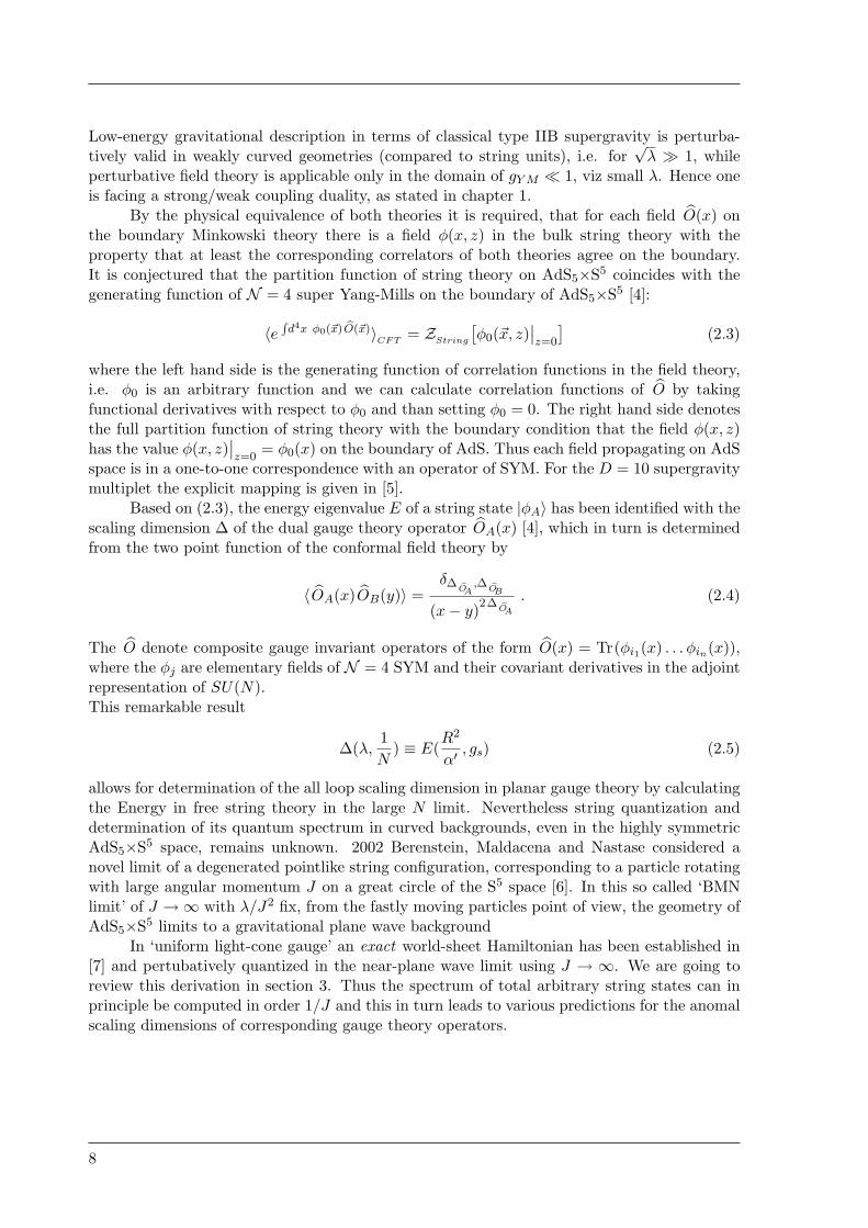


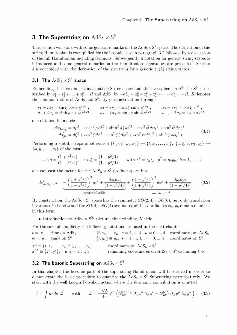
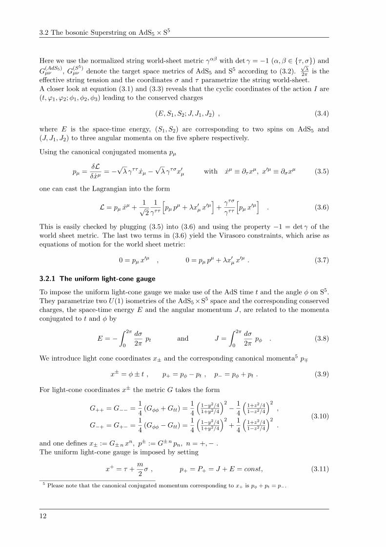


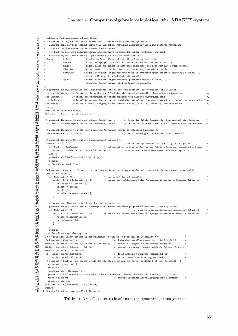


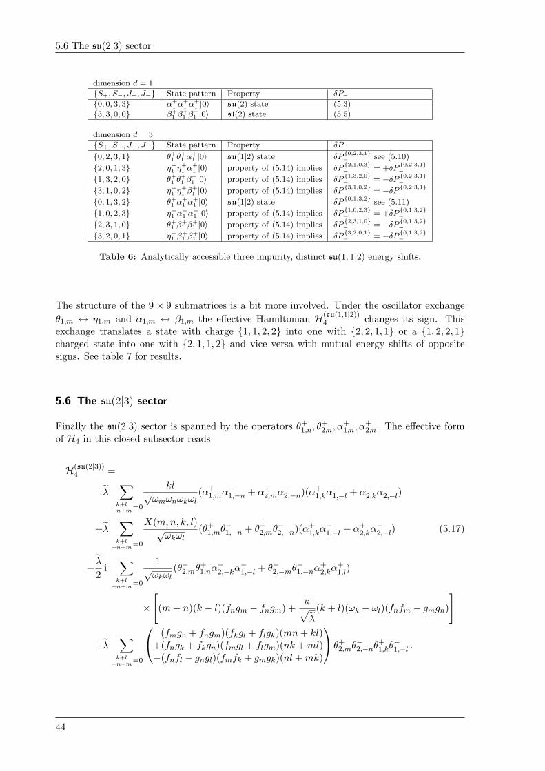
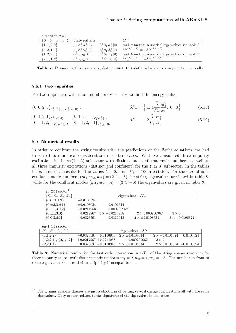


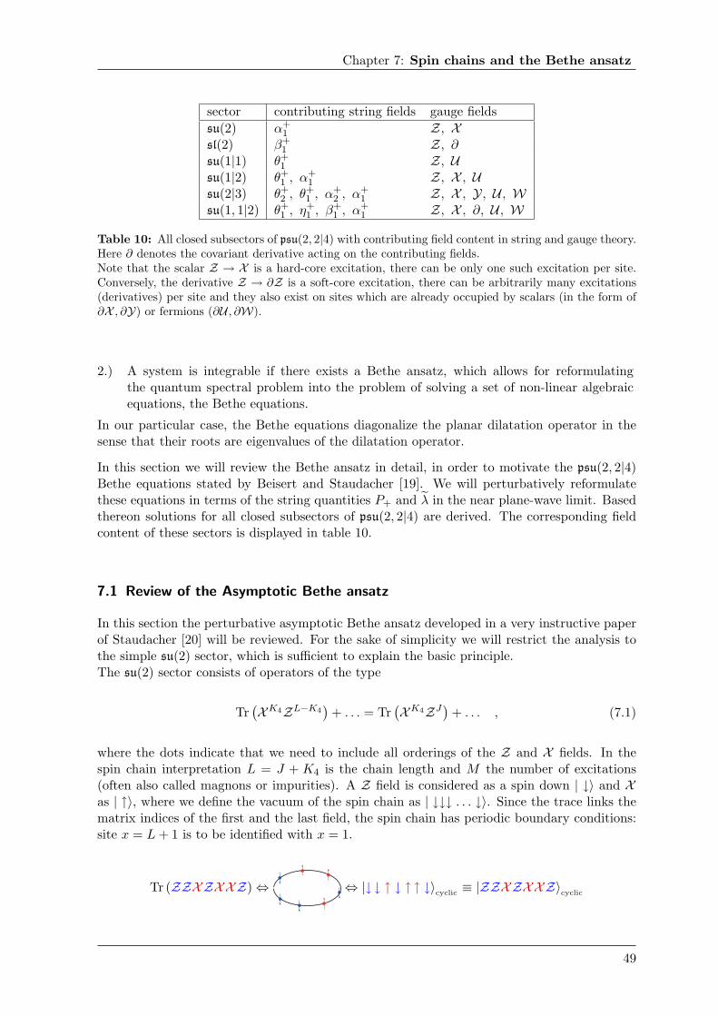


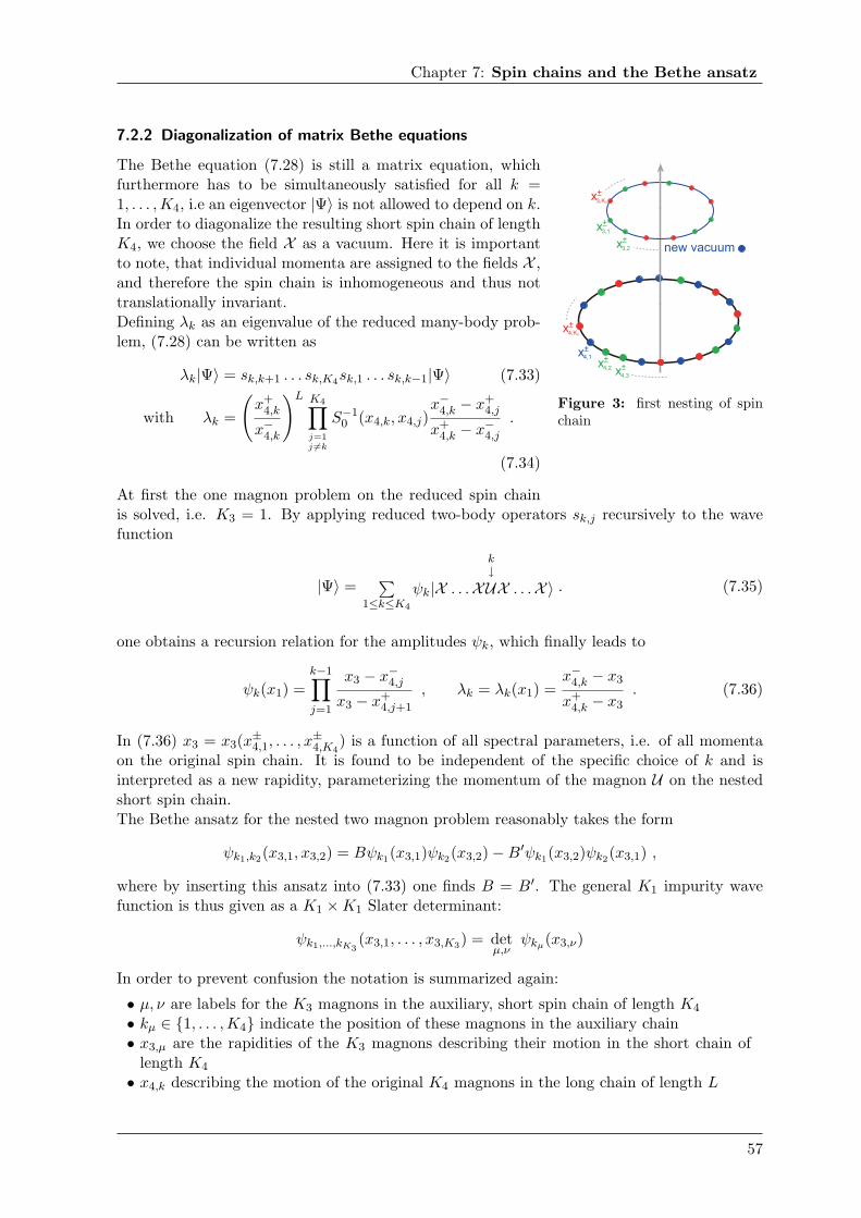


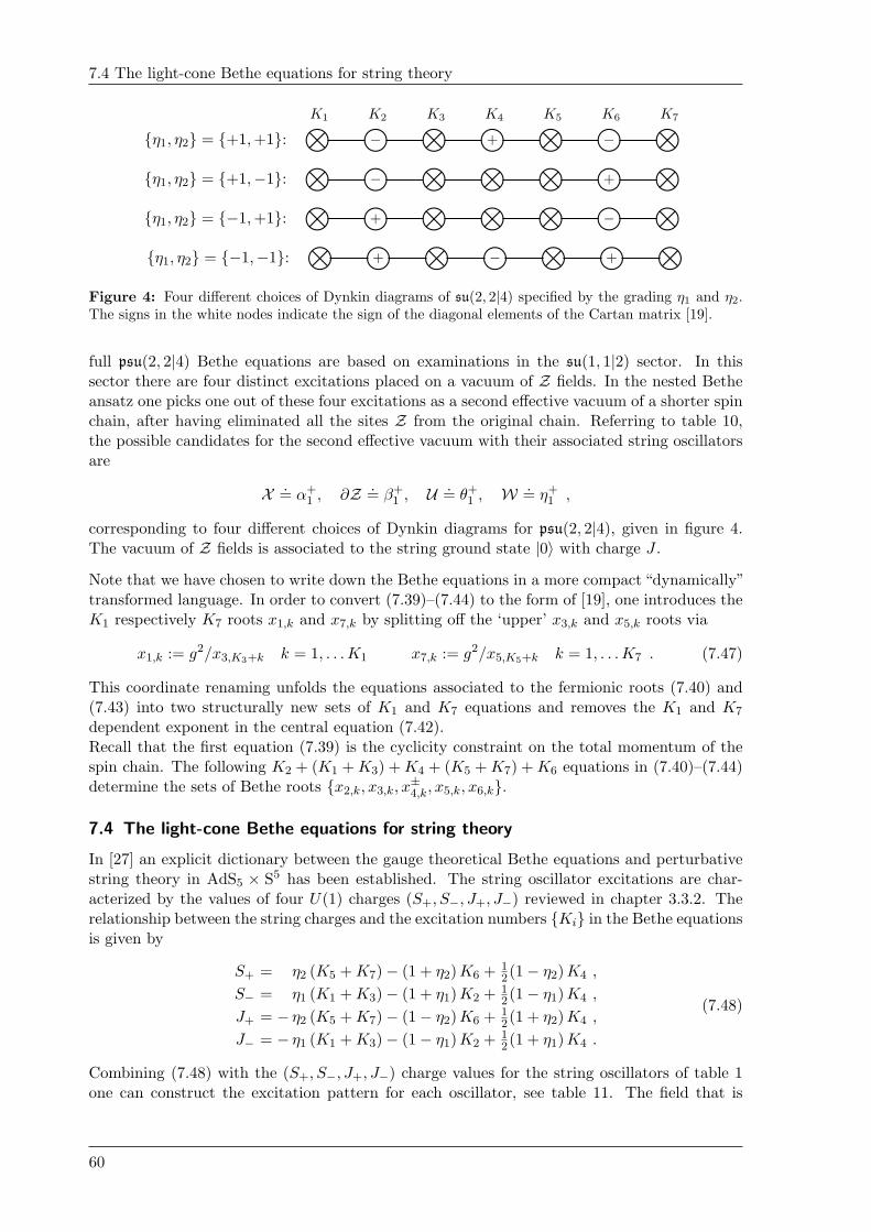
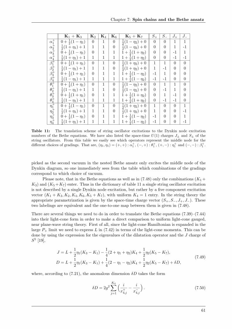


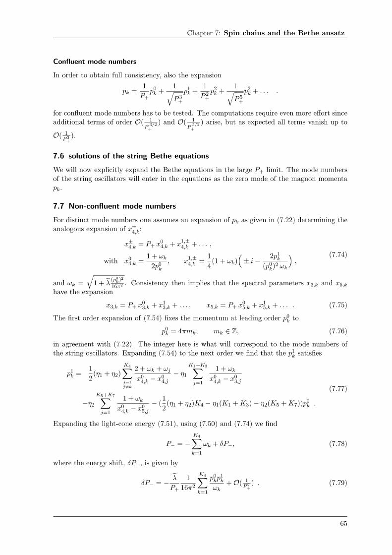
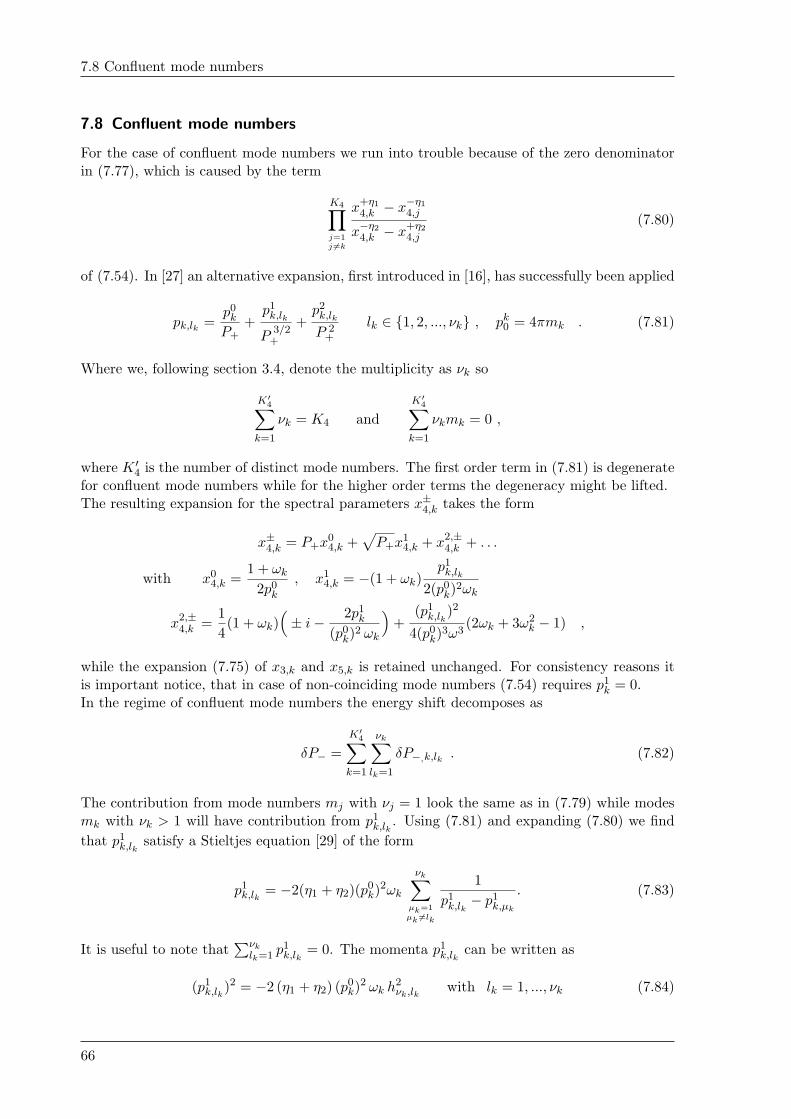


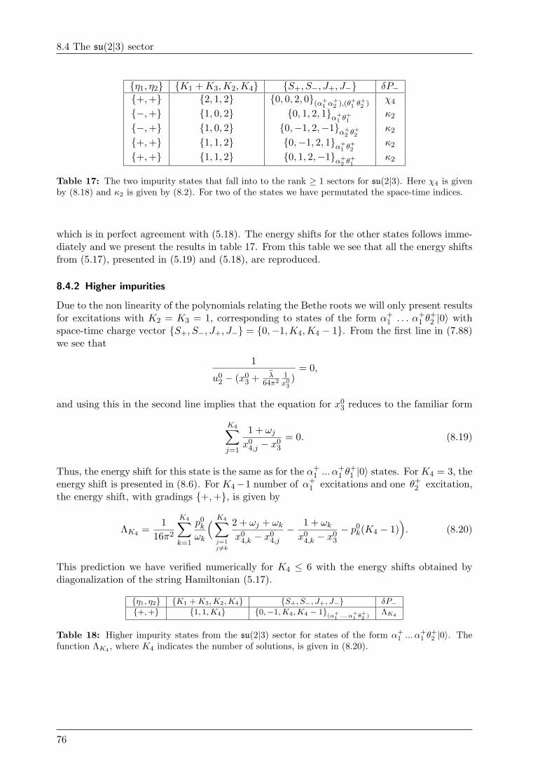


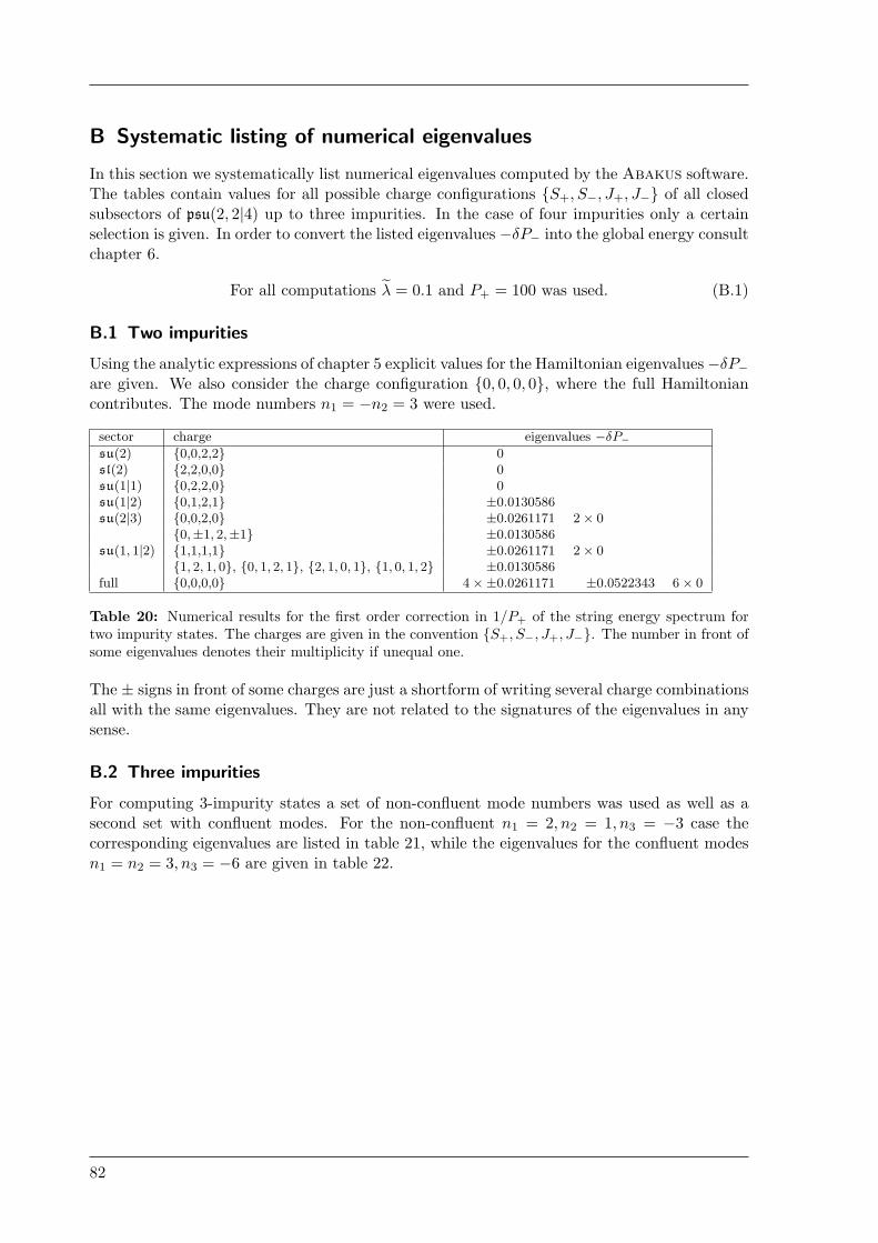


![cardchecklist 391105 script · CIR acp s5-21 ON S5-36 a SPR S5-41 s5-77 DR S5-58 a R S5-5 acp OSPR S5-22 ON S5-37 C] S5-42 acp DR CIR apR a R S5-27 C] PR S-5-88 a R S5-47 CIN s5-64](https://static.documents.pub/doc/80x56/5f34fee96b83591bd77e360b/cardchecklist-391105-script-cir-acp-s5-21-on-s5-36-a-spr-s5-41-s5-77-dr-s5-58-a.jpg)


![T-dualization of type II superstring theory in double space2.1 Type II superstring in pure spinor formulation The sigma model action for the type II superstring of Ref. [45]isoftheform](https://static.documents.pub/doc/80x56/5f62f88e1bd1cb48213457dc/t-dualization-of-type-ii-superstring-theory-in-double-space-21-type-ii-superstring.jpg)


