INTEGRAL REPRESENTATIONS OF AUTOMORPHIC L-FUNCTIONS …math.columbia.edu/~yihang/minor thesis/minor...

INTEGRAL REPRESENTATIONS OF AUTOMORPHICL-FUNCTIONS USING AUTOMORPHIC DISTRIBUTIONS

YIHANG ZHU

Abstract. This is an exposition of the theory of automorphic distributions,mirabolic Eisenstein distributions, and their pairings, which is developed byStephen Miller andWilfried Schmid in [MS04], [MS06], [MS08], [MS11], [MS12a],[MS12b], [MS12c]. We report on the application of this theory to the study ofexterior square automorphic L-functions for GL2n over Q in [MS12a].

Contents

Introduction 20.1. Notations and conventions 40.2. Acknowledgments 41. Automorphic distributions 41.1. Basic definitions 51.2. Concrete realization using Casselman-Wallach embeddings 61.3. Whittaker-Fourier expansion 71.4. The Whittaker distributions 82. Mirabolic Eisenstein distributions 92.1. Basic definitions 92.2. Fourier expansion and analytic continuation 122.3. Functional equation 133. Automorphic pairings 153.1. General setting 163.2. The special case related to exterior square L-functions 173.3. Inherited functional equation 204. Adelization 214.1. Adelization of an automorphic distribution 214.2. Adelic Whittaker-Fourier expansion 224.3. Adelic construction of Eisenstein distributions 244.4. Adelization of the automorphic pairing 275. The exterior square L-function 295.1. Overview 295.2. Unfolding of the automorphic pairing 315.3. Calculation of Ψ∞(s,wλ,δ) 335.4. Functional equation and full holomorphy 405.5. Historical remarks 41References 42

1

2 YIHANG ZHU

Introduction

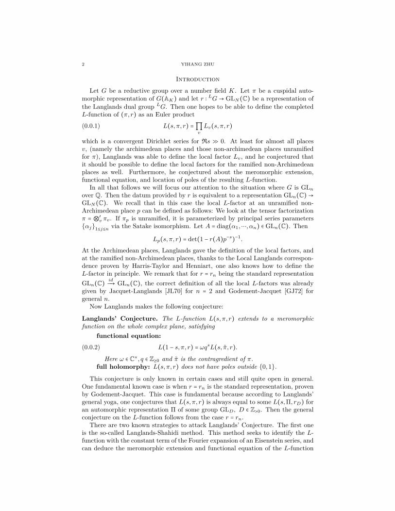
Let G be a reductive group over a number field K. Let π be a cuspidal auto-morphic representation of G(AK) and let r ∶ LG→ GLN(C) be a representation ofthe Langlands dual group LG. Then one hopes to be able to define the completedL-function of (π, r) as an Euler product

L(s, π, r) =∏v

Lv(s, π, r)(0.0.1)

which is a convergent Dirichlet series for Rs ≫ 0. At least for almost all placesv, (namely the archimedean places and those non-archimedean places unramifiedfor π), Langlands was able to define the local factor Lv, and he conjectured thatit should be possible to define the local factors for the ramified non-Archimedeanplaces as well. Furthermore, he conjectured about the meromorphic extension,functional equation, and location of poles of the resulting L-function.

In all that follows we will focus our attention to the situation where G is GLnover Q. Then the datum provided by r is equivalent to a representation GLn(C)→GLN(C). We recall that in this case the local L-factor at an unramified non-Archimedean place p can be defined as follows: We look at the tensor factorizationπ = ⊗′

v πv. If πp is unramified, it is parameterized by principal series parameters{αj}1≤j≤n via the Satake isomorphism. Let A = diag(α1,⋯, αn) ∈ GLn(C). Then

Lp(s, π, r) = det(1 − r(A)p−s)−1.

At the Archimedean places, Langlands gave the definition of the local factors, andat the ramified non-Archimedean places, thanks to the Local Langlands correspon-dence proven by Harris-Taylor and Henniart, one also knows how to define theL-factor in principle. We remark that for r = rn being the standard representationGLn(C) idÐ→ GLn(C), the correct definition of all the local L-factors was alreadygiven by Jacquet-Langlands [JL70] for n = 2 and Godement-Jacquet [GJ72] forgeneral n.

Now Langlands makes the following conjecture:

Langlands’ Conjecture. The L-function L(s, π, r) extends to a meromorphicfunction on the whole complex plane, satisfying

functional equation:

L(1 − s, π, r) = ωqsL(s, π, r).(0.0.2)

Here ω ∈ C×, q ∈ Z≥0 and π is the contragredient of π.full holomorphy: L(s, π, r) does not have poles outside {0,1}.

This conjecture is only known in certain cases and still quite open in general.One fundamental known case is when r = rn is the standard representation, provenby Godement-Jacquet. This case is fundamental because according to Langlands’general yoga, one conjectures that L(s, π, r) is always equal to some L(s,Π, rD) foran automorphic representation Π of some group GLD, D ∈ Z>0. Then the generalconjecture on the L-function follows from the case r = rn.

There are two known strategies to attack Langlands’ Conjecture. The first oneis the so-called Langlands-Shahidi method. This method seeks to identify the L-function with the constant term of the Fourier expansion of an Eisenstein series, andcan deduce the meromorphic extension and functional equation of the L-function

INTEGRAL REPRESENTATIONS OF L-FUNCTIONS USING DISTRIBUTIONS 3

from the analytic properties of the Eisenstein series. The disadvantage of thismethod is that it cannot provide a proof of full holomorphy of the L-function.

The second method is the method of integral representation. Roughly speaking,this method seeks to express the L-function as an integral of some automorphicforms against some kernel depending on s, over a certain space. Then the analyticproperties of the L-function can be deduced from those of the kernel. This methoddates back to the classical works by Wilton, Hecke, Maass, and Ranking-Selbergon first and second order L-functions of modular and Maass forms, and was laterdeveloped by Jacquet, Shalika, Piatetski-Shapiro, et al. Notably for us, the theoryfor the exterior square L-function L(s, π,Ext2⊗χ) is worked out in Jacquet-Shalika[JS90]. Here Ext2 means the anti-symmetric square of the standard representationrn and χ is a Dirichlet character. This method also has disadvantages. Firstly, thefunctional equation produced by this involves some "archimedean integrals" thatone desires to eliminate in order to get a functional equation of the form (0.0.2),but these integrals may be too difficult to compute. Secondly, since the analyticproperties of these "archimedean integrals" are hard to explicate, it is also difficultto prove full holomorphy by this method.

This paper is an exposition of a variant of the integral representation method,developed by Stephen Miller and Wilfried Schmid in the past decade in a seriesof papers [MS04], [MS06], [MS08], [MS11], [MS12a], [MS12b], [MS12c]. Instead ofconsidering automorphic forms in a cuspidal automorphic representation π, theyassociate an automorphic distribution τ to π. The object τ is a roughly speakinga family {τgf }gf ∈G(Af )

of distributions on G(R), with each of its members τgfsatisfying an automorphy condition with respect to an arithmetic subgroup ofG(R).Then π can be reconstructed from the knowledge of τ . Miller and Schmid developeda theory of pairings between these objects, which can be viewed as an analogyof the integrals of products of automorphic forms. The pairings also work forobjects similar to these automorphic distributions, namely the mirabolic Eisensteindistributions, which heuristically are the analogous counterpart for Eisenstein series.Thus one can seek to relate these pairings to automorphic L-functions, just as in theclassical method of integral representation. In particular, in analogy to the workof Jacquet-Shalika [JS90] mentioned above, this method also allows one to studyL(s, π,Ext2⊗χ). It turns out that the resulting "archimedean integrals" using thismethod become possible to compute, in contrast to the classical method. Usingthis method, in [MS12a] Miller and Schmid proved for G = GL2n over Q the fullholomorphy of LS(s, π,Ext2⊗χ), where S is a finite set of places required to containthe ramified non-archimedean places, and LS means the partial L-function definedby excluding the local factors corresponding to v ∈ S from the product (0.0.1). Wewill present the content of [MS12a] in detail in the following.

We say some words about the organization of this paper. In §1 we introducethe concept of automorphic distributions and discuss how to use a Casselman em-bedding into a principal series to realize the automorphic distribution as a moreconcrete distribution on a manifold. We also discuss the Whittaker-Fourier expan-sion of an automorphic distribution. In §2 we establish the theory of mirabolicEisenstein distributions, which is an analogue of the theory of Eisenstein series.We discuss the Fourier expansion, analytic continuation, and functional equationof these Eisenstein distributions. In §3 we discuss the main analytic tool of the

4 YIHANG ZHU

Miller-Schmid method, namely an invariant pairing between automorphic distribu-tions. The pairing is an analogue of the Rankin-Selberg type integral considered inmore classical works. We will describe the specific pairing that will be used to studyexterior square L-functions. This pairing has the Eisenstein distribution consideredin §2 as one of its variables and in particular inherits the analytic properties of theEisenstein distribution, such as analytic continuation and functional equation. In§4 we put the previous material into an adelic language, which is more suited tostudy the L-function when the automorphic representation in question is not nec-essarily unramified at all finite primes. In §5 we use the theory developed beforeto study the exterior square L-function. We discuss the main result of [MS12a] onthe full holomorphy of the exterior square L-function. We show that the specificautomorphic pairing considered before equals to an archimedean integral times apartial Euler product for the exterior square L-function. This is a generalizationof the integral representation of Jacquet-Shalika. We show how to calculate thearchimedean integral in this case.

The main references for this paper are [MS11] and [MS12a].

0.1. Notations and conventions. In §§1, 2, 3, notations like G,B,N,P,U willdenote real Lie groups. In §§4, 5, the same notations will denote the correspond-ing algebraic groups over Q, and their groups of real points will be denoted byG(R),B(R), etc. Notations X,Y,Xn, Yn will always mean flag varieties in thecontext of real Lie groups, so that they are real manifolds.

Without further specification, parabolic subgroups B,P, P will always consist of(block) lower triangular matrices in GLn, and unipotent subgroups N,U, U willalways consist of (block) upper triangular unipotent matrices. In the contextof automorphic pairings, the notation U will be reserved to mean the subgroup

( In Mn×n

In) ⊂ GL2n, and the mirabolic subgroups which used to be denoted by

U will be denoted by Un.When we consider L-functions, we will not follow the convention of using Λ to

denote the completed L-function (i.e. including the infinite places) and using Lto denote the Euler product over finite primes. Instead, for us L means the Eulerproduct over all the places, and LS means the Euler product over all the placesnot in S, where S is any finite set of places.

0.2. Acknowledgments. This paper is the author’s minor thesis for the HarvardMathematics Ph.D. program. The author wholeheartedly thanks his minor thesisadvisor, Professor Wilfried Schmid, for explaining the essential points of the subjectto him and answering his questions patiently and detailedly. He also thanks Chen-glong Yu and Boyu Zhang for answering his questions about analysis and havingseveral helpful discussions with him. Last but not least, he would like to expresshis gratitude to Han Wu, for all her support and encouragement during the writingof the paper.

1. Automorphic distributions

In this section we discuss the concept of an automorphic distribution. We willuse the classical language in terms of real Lie groups and their arithmetic sub-groups. This already suffices in the study of automorphic representations that are


unramified at each non-archimedean place. Later we will re-organize things in anadelic language.

1.1. Basic definitions. Let G be a real Lie group which is the set of real points ofa reductive algebraic group defined over Q. Let Γ be an arithmetic subgroup. Wefix a Haar measure d g on G. We also fix a unitary character on the center Z of G

ω ∶ Z → S1 ⊂ C.

Then we can consider the Hilbert space

L2ω(Γ/G) ∶= {f ∈ L2

loc(Γ/G)∣f(gz) = ω(z)f(g) for z ∈ Z, and ∫Γ/G/Z

∣f ∣2 d g <∞} .

The group G acts on L2ω(Γ/G) unitarily via right translation. By a classical auto-

morphic representation with central character ω we will mean an irreducible unitaryrepresentation (π,V ) of G together with a G-equivariant embedding

j ∶ V ↪ L2ω(Γ/G).

For such a V , we will denote by V ∞ ⊂ V its subset of smooth vectors. These arethe vectors v ∈ V for which the map

evv ∶ G ∋ g ↦ gv ∈ Vis smooth. By identifying v ∈ V ∞ with evv we get an identification

V ∞ ∼Ð→ C∞(G,V ).

Thus V ∞ inherits the Fréchet topology on C∞(G,V ). Let (π′, V ′) be the repre-sentation of G contragredient to (π,V ). Then we define the space of distributionvectors on V to be the space of continuous linear functionals on V ′∞. This spacewill be denoted by V −∞. Thus we have

V ∞ ⊂ V ⊂ V −∞,

and similarlyV ′∞ ⊂ V ′ ⊂ V ′−∞.

This is compatible with the following convention: for a smooth manifold M , we de-fine the space C−∞(M) of distributions on M to be the space of continuous linearfunctionals on the Fréchet space of smooth compactly supported measures on M(i.e. smooth compactly supported sections of the determinant bundle). More gen-erally, if L is a vector bundle on M , we define the space C−∞(M,L) of distributionsections of L to be

C∞(M,L)⊗C∞(M) C−∞(M).

We come back to the classical automorphic representation (π,V, j). Since thesmoothness of a vector can be read off from the G-action on it, for v ∈ V ∞, thevector j(v) ∈ L2

ω(Γ/G) is also smooth. But this means j(v) is a smooth functionon Γ/G. Thus we can define a functional on V ∞ as follows:

τ ∶ V ∞ ∋ v ↦ j(v)(e) ∈ C.Here e is the identity element in G. This functional τ is continuous and Γ-invariant.Hence by definition

τ ∈ (V ′−∞)Γ.(1.1.1)

6 YIHANG ZHU

We call τ the automorphic distribution associated to (π,V, j). Note that the datum(π′, V ′, τ ∈ V ′−∞) recovers (π,V, j) completely. In fact, firstly (π,V ) as an abstractrepresentation is recovered by (π′, V ′) as its contragredient. Secondly the embed-ding j is recovered from j∣V∞ since V ∞ is dense in V , and j∣V∞ is recovered fromτ using the relation

j(v)(g) = j(π(g)v)(e) = τ(π(g)v), for v ∈ V ∞, g ∈ G.

1.2. Concrete realization using Casselman-Wallach embeddings. We spe-cialize the situation to G = GLn(R), and Γ ⊂ G is an arithmetic subgroup as before.Let B ⊂ G be the subgroup of lower triangular invertible matrices and N ⊂ G be thesubgroup of upper triangular matrices with 1’s on the diagonal. In the followingwe describe how to realize an automorphic distribution (1.1.1) considered above ina more concrete way, namely, as a distribution on G satisfying some automorphyconditions, as well as a distribution on the manifold (Γ ∩N)/N .

The main tool used here is the Casselman-Wallach embedding of an irreducibleunitary representation into a principal series. The principal series are representa-tions of G induced from characters of B. For parameters (λ, δ) ∈ Cn × (Z/2Z)n, wedefine a character on B

χλ,δ ∶ B → C×, (bij)↦ ∏1≤j≤n

sgn(bj)δj ∣bj ∣λj .

Let ρ = (n−12 , n−3

2 ,⋯, 1−n2 ) ∈ Cn. Thus χρ,0 corresponds to the half sum of the simple

roots associated to the Borel B and the diagonal torus. We define the principalseries representations Vλ,δ of G as the (unnormalized) induction from B to G ofχλ−ρ,δ. The resulting representation is not necessarily unitary, so we may justview Vλ,δ as a Harish-Chandra module and consider its various globalizations. Inparticular we have globalizations inside the space of smooth functions on G andinside the space of distributions on G:

V ∞λ,δ = {f ∈ C∞(G)∣f(gb) = χλ−ρ,δ(b)−1f(g) for b ∈ B,g ∈ G}

V −∞λ,δ = {f ∈ C−∞(G)∣f(gb) = χλ−ρ,δ(b)−1f(g) for b ∈ B,g ∈ G} .

Here of course we have abused notation when writing the transformation conditionfor f ∈ C−∞(G). Alternatively, the character χλ−ρ,δ on B defines a line bundleLλ−ρ,δ on the flag variety X = G/B, and we have natural identifications

V ∞λ,δ ≅ C∞(X,Lλ−ρ,δ)

V −∞λ,δ ≅ C−∞(X,Lλ−ρ,δ).

On choosing the canonical measure d g on the compact manifold X induced fromthe Haar measure d g on G, we get a dual pairing between V −∞

λ,δ and V ∞−λ,δ.

Now since N ∩B = {e}, the map N → X = G/B is injective. It can be seen thatit is an open embedding with dense image. We call its image the open Schubertcell and identify it with N . The line bundle Lλ−ρ,δ is canonically trivialized on theopen Schubert cell, so we have restriction maps

V ∞λ,δ → C∞(N)(1.2.1)

V −∞λ,δ → C−∞(N).(1.2.2)

The first map is injective since N is dense in X, but the second map is not injectivesince a distribution cannot be determined by its restriction to a dense open subset.An example is a δ function/section supported at a point outside the open set.


The results of Casselman and Wallach [Cas80][Cas89][Wal83] imply that for anyirreducible unitary representation (π′, V ′) of G, there exists a principal series rep-resentation Vλ,δ such that there exist G-equivariant embeddings

V ′∞ ↪ V ∞λ,δ,(1.2.3)

V ′−∞ ↪ V −∞λ,δ .(1.2.4)

For details concerning this see [MS12b].Now given any element τ ∈ (V ′−∞)Γ, in particular τ can be an automorphic

distribution considered above, we choose (λ, δ) to have embeddings (1.2.3) and(1.2.4). By composing (1.2.4) with (1.2.2) we map τ to an element

τ ∈ C−∞(N)N∩Γ = C−∞((N ∩ Γ)/N).(1.2.5)

Though the map (1.2.2) is not injective, we observe that the Γ-translates of theopen Schubert cell cover X, so, by insisting that τ be invariant under Γ, we canconsider τ as an element of C−∞((N ∩ Γ)/N) with no loss of information.

1.3. Whittaker-Fourier expansion. Now we consider the abelianization Nab ∶=N/[N,N] ofN . Here [N,N] is the derived subgroup ofN . We have an isomorphismof Lie groups

Rn−1 ∼Ð→ N/[N,N](1.3.1)

x = (xi)↦ n(x) =

⎛⎜⎜⎜⎜⎜⎝

1 x11 x2

⋱ ⋱1 xn−1

1

⎞⎟⎟⎟⎟⎟⎠

The subgroup Γ∩N is arithmetic inN , hence co-compact, and similarly Γ∩[N,N]is co-compact in [N,N]. Hence we can "average" our τ ∈ C−∞((Γ ∩N)/N) over(Γ ∩ [N,N])/[N,N] to get the "abelian component" of τ . Define

τab ∶= vol((Γ ∩ [N,N])/[N,N])−1 ∫(Γ∩[N,N])/[N,N]

l(n)τ dn.(1.3.2)

As before, we may either view τab as an element in V −∞λ,δ , or an element in C−∞((Γ∩

N)/N) via restriction to N . The latter element by construction lies inside

C−∞([N,N](Γ ∩N)/N).

Note that the space [N,N](Γ ∩N)/N is isomorphic to Rn−1 modulo a lattice viathe identification (1.3.1). Any distribution on such a torus is an infinite linearcombination of the standard trigonometric characters on it. We write

τab(n(x)) = ∑k∈Qn−1

cke(k1x1 +⋯kn−1xn−1).(1.3.3)

Here ck is nonzero only for k ∈M−1Z where M is a fixed positive integer dependingon Γ, and we use the notation

e(z) ∶= e2πiz.(1.3.4)

We make a few remarks. Firstly, we define the cuspidal condition for elementsin (V ′−∞)Γ. We say τ ∈ (V ′−∞)Γ is cuspidal, if for any U ⊂ G that is the unipotent

8 YIHANG ZHU

radical of a proper parabolic subgroup of G defined over Q, we have

∫U/(Γ∩U)

π′(u)τ du = 0.(1.3.5)

Suppose we start with a classical automorphic representation j ∶ V ↪ L2ω(Γ/G) that

is cuspidal. This means that j(V ∞) consists of smooth functions F satisfying theusual cuspidal conditions

∫Γ∩U/U

F (ug)du = 0(1.3.6)

for all g ∈ G and U ⊂ G as in (1.3.5). Then the associated automorphic distribu-tion τ ∈ (V ′−∞)Γ is cuspidal. This has the following implications on the Fouriercoefficients ck: If k = (kj) ∈ Qn−1 where kj = 0 for some j, then ck = 0.

Secondly, the Fourier coefficients ck in (1.3.3) a priori depends on the choice of theembedding (1.2.4), but we will see later that after a normalization (which dependson (λ, δ)), they become dependent only on the classical automorphic representation(V, j). The normalized Fourier coefficients are defined as

ak ∶= ckn−1∏j=1

(sgnkj)δ1+⋯+δj ∣kj ∣λ1+⋯+λj .(1.3.7)

Later we will need the contragredient picture as well. We name the importantmatrix

wlong ∶=⎛⎜⎝

1⋰

1

⎞⎟⎠.(1.3.8)

Consider the outer automorphism of Gg ↦ g ∶= wlong(gt)−1wlong

−1.(1.3.9)We use this to pull back τ ∈ C−∞(G) to get another element τ ∈ C−∞(G). Abusingnotation, we have

τ(g) = τ(g).(1.3.10)

Now if τ ∈ (V −∞λ,δ )Γ as before, then

τ ∈ (V −∞

λ,δ)Γ,

where Γ is the image of Γ under (1.3.9), andλ = (−λn,−λn−1,⋯, λ1), δ = δ.

The Fourier coefficients ck and ck of τ and τ respectively in (1.3.3) are related byc(k1,⋯,kn−1) = c(−kn−1,⋯,−k1).(1.3.11)

1.4. The Whittaker distributions. We consider the problem of extending theexpansion (1.3.3) from the open Schubert cell N to X = G/B.

Consider the composed functionN Ð→ Nab Ð→ C(1.4.1)n↦ n(x)↦ e(x) = e(x1 +⋯xn−1).(1.4.2)

This function is not compactly supported on N , and cannot be extended to asmooth function on X. However, it does canonically extend to a distribution inV −∞λ,δ . For details see [CHM00]. We denote by wλ,δ ∈ V −∞

λ,δ the extension, and call


it the Whittaker distribution. Of course wλ,δ restricted to NB ⊂ G is the functiongiven by the following formula, which is just the transformation rule defining Vλ,δ:

wλ,δ

⎛⎜⎜⎜⎜⎜⎝

⎛⎜⎜⎜⎜⎜⎝

1 x1 ∗ ∗ ∗1 x2 ∗ ∗

⋱ ∗ ∗1 xn−1

1

⎞⎟⎟⎟⎟⎟⎠

⎛⎜⎜⎜⎜⎜⎝

b1∗ b2∗ ∗ ⋱∗ ∗ ∗ bn−1∗ ∗ ∗ ∗ bn

⎞⎟⎟⎟⎟⎟⎠

⎞⎟⎟⎟⎟⎟⎠

(1.4.3)

= e(x1 +⋯ + xn−1)n

∏j=1

∣bj ∣(n+1)/2−j−λj sgn(bj)δj .

For the other terms e(kx), we assume k = (k1,⋯kn−1) with each kj nonzero. Notethat if τ is cuspidal, then the nonzero terms appearing in (1.3.3) all have index kwith this property, as we remarked before. LetD(k) = diag(k1⋯kn−1, k2⋯kn−1,⋯,1).Then conjugation by D(k) transforms (1.4.1) to n↦ n(x)↦ e(k1x1+⋯+kn−1xn−1).Therefore the canonical extension of the latter is given by

wλ,δ(D(k)gD(k)−1) (1.4.3)= wλ,δ(D(k)g)n−1∏j=1

(n−1∏i=j

∣ki∣−(n−1)/2+j+λjj

∏i=1kδii ).(1.4.4)

Combining (1.4.4) and (1.3.7), we can rewrite (1.3.3) as

τab(g) = ∑k∈Qn−1

ak

∏n−1j=1 ∣kj ∣j(n−1)/2wλ,δ(D(k)g).(1.4.5)

This is the Whittaker Fourier expansion for the distribution τab.

2. Mirabolic Eisenstein distributions

In analogy to the classical Rankin-Selberg method, where Eisenstein series areused as the integration kernels of the integral representation of the L-function, themethod of Miller-Schmid studies certain pairings between automorphic distribu-tions and Eisenstein distributions. The Eisenstein distributions are distributionalanalogues of classical Eisenstein series. In this section we define them and discusstheir properties using the classical language in terms of GLn(R) and its arithmeticsubgroups. Later in 4.3 we will give an adelic construction of Eisenstein distri-butions as some adelic distributions, but their analytic properties reduce to thediscussion here.

2.1. Basic definitions. In the following we define two completely parallel versionsof objects, one un-tilde version and one tilde version. The theory for these twoversions are parallel and can be related using the matrix wlong defined in (1.3.8).We first consider the following mirabolic subgroups of G = GLn(R).

P ∶= ( GL1(R) 0∗ GLn−1(R) ) , P ∶= ( GLn−1(R) 0

∗ GL1(R) ) .

We also consider their opposite unipotent radicals

U ∶= ( 1 ∗0 In−1

) , U ∶= ( In−1 ∗0 1 ) .

These subgroups are related byP = wlong(P )twlong, U = wlong(U)twlong,

10 YIHANG ZHU

i.e. by the outer automorphism g ↦ g defined in (1.3.9).Define the generalized flag varieties

Y ∶= G/P, Y ∶= G/P .

The projection maps U → Y and U → Y are open embeddings with dense image,and we call their images the open Schubert cells. For parameters (ν, ε) ∈ C ×Z/2Z,we define characters

χν,ε ∶ P → C×, ( a⋮ B

)↦ ∣a∣(n−1)νn sgn(a)ε ∣detB∣−ν/n , a ∈ R×, B ∈ GLn−1(R)

χν,ε ∶ P → C×, ( B⋯ a

)↦ ∣a∣−(n−1)νn sgn(a)ε ∣detB∣ν/n , a ∈ R×, B ∈ GLn−1(R).

Let ρmir = n2 . Similarly to what we have done before, we can define the degenerate

principal series Wν,ε and Wν,ε as inductions of χν−ρmir,ε and χν−ρmir,ε from P and Pto G respectively. The characters χν−ρmir,ε and χν−ρmir,ε define line bundles Lν−ρmir,ε

and Lν−ρmir,ε on Y and Y respectively. The space of smooth vectors inside Wν,ε isidentified with

W∞ν,ε = C∞(Y,Lν−ρmir,ε) = {f ∈ C∞(G)∣f(gp) = χν−ρmir,ε(p)−1f(g), for g ∈ G,p ∈ P}

Similarly for the space of distribution vectors and the tilde version.On the open Schubert cell U , the line bundle Lν−ρmir is canonically trivial, so

distribution sections of Lν−ρmir on U are just scalar distributions. Consider the deltafunction at identity δe as such a distribution on U . It is compactly supported, sowe can extend it by zero to get an element δe ∈W −∞

λ,ε . Define

δ∞ ∶= l(wlong)δe ∈W −∞λ,ε .

The distribution section δ∞ is supported on the point wlongP ∈ Y . Similarly wedefine δ∞ ∈ W −∞

λ,ε which is supported on the point wlongP ∈ Y .For our later purpose, it suffices to define and study mirabolic Eisenstein series

in this classical language only for the following congruence subgroups

Γ = Γ0(N) = {γ ∈ GLn(Z)∣N divides γn,j ,1 ≤ j ≤ n − 1}Γ = Γ0(N) = {γ ∈ GLn(Z)∣N divides γj,1,2 ≤ j ≤ n} .

In our theory we allow twisting by a Dirichlet character modulo N . Let

ψ ∶ (Z/NZ)× → C×

be such one. We assume

ψ(−1) = (−1)ε,(2.1.1)

We define characters

α ∶ Γ→ C×, γ ↦ ψ(γnn)−1(2.1.2)α ∶ Γ→ C×, γ ↦ ψ(γ11).

Thus α(γ) = α(γ).Let Γ∞ = Γ∩wlongPwlong = GLn(Z)∩wlongPwlong ⊂ Γ be the stabilizer of wlongP ∈

Y in Γ. If γ = (γij) ∈ Γ∞, then γnn = ±1, and

l(γ)δ∞ = γεnnδ∞.(2.1.3)


We define the mirabolic Eisenstein distributionEν,ψ ∶= L(ν +

n

2, ψ) ∑

γ∈Γ/Γ∞α(γ)l(γ)δ∞.(2.1.4)

This is an infinite sum in the space W −∞ν,ε . The parameter ε is omitted from the

notation Eν,ψ just for brevity. We see that the parity condition (2.1.1) togetherwith (2.1.2) and (2.1.3) guarantees that α(γ)l(γ)δ∞ = δ∞ for γ ∈ Γ∞, so (2.1.4) isat least formally well defined.

In fact when Rν > 1/2 this series (2.1.4) converges in the strong distributiontopology (i.e. the topology of uniform convergence on bounded subsets of theFréchet space of test measures). Thus in this case we get an element Eν,ψ ∈ V −∞

ν,ε .If we view Eν,ψ as a family of elements in C−∞(G), then the dependence on ν isholomorphic forRν > n/2. This means that for a fixed smooth compactly supportedfunction f on G, the function

{Rν > n/2} ∋ ν ↦ ∫GEν,ψ(g)f(g)d g

is holomorphic.We briefly explain why we have the asserted convergence and holomorphic de-

pendence. Firstly we restrict (2.1.4) to the open Schubert cell U ⊂ Y . Thus we geta series of scalar distributions on U . An elementary and formal computation showsthat this series is equal to

Eν,ψ(u1,⋯, un−1) = ∑v∈Zn,v1>0,N ∣vi

ψ(vn)v−ν−n/21 δvn/v1(u1)⋯δv2/v1(un−1),(2.1.5)

where we identify U with Rn−1 via

⎛⎜⎜⎜⎝

1 un−1 ⋯ u11

⋱1

⎞⎟⎟⎟⎠↦ (u1,⋯, un−1).(2.1.6)

Take f ∈ C∞c (U) = C∞

c (Rn−1) to be a test function. By (2.1.5), formally we have

∫UEν,ψ(u)f(u)du = ∑

v∈Zn,v1>0,N ∣vi

ψ(vn)v−ν−n/21 f(vn/v1, vn−1/v1,⋯, v2/v1).(2.1.7)

Since f is compactly supported, there exists a constant Cf > 0, depending only onthe size of the support of f in Rn−1, such that for each fixed v1 ∈ Z>0, there exists atmost (Cfv1)n−1 points (v2,⋯, vn) ∈ Zn−1 such that f(vn/v1, vn−1/v1,⋯, v2/v1) ≠ 0.Let Mf ∶= sup(∣f ∣). Then the series in (2.1.7) is majorized by

∑v1>0,N ∣v1

v−ν−n/21 (Cfv1)n−1Mf = ∑

v1>0,N ∣v1

Cn−1f Mfv

n/2−ν−11 .(2.1.8)

When Rν > n/2, this series (2.1.8) converges absolutely, and uniformly with respectto f , provided that Cf and Mf are bounded. This shows the convergence of (2.1.4)in the strong distribution topology, at least when everything is restricted to U ⊂Y . Also the expression (2.1.7) shows holomorphic dependence with respect to ν.The full statements about convergence and holomorphic dependence (i.e. not justthe statements about restrictions to U) follow from the observation that (2.1.4)is invariant under the congruence subgroup Γ1(N) ∶= ker(α) ⊂ Γ, and the Γ1(N)-translates of the open Schubert cell U cover Y .

12 YIHANG ZHU

By construction we havel(γ)Eν,ψ = α(γ)−1Eν,ψ, γ ∈ Γ.

This is the "automorphy property" under Γ satisfied by the Eisenstein distribution.Analogously, we define

Eν,ψ ∶= L(ν +n

2, ψ) ∑

γ∈Γ/Γ∞

α(γ)l(γ)δ∞.(2.1.9)

The same as before, when Rν > n/2, the series converges in the strong distributiontopology and gives an element Eν,ψ ∈ W −∞

ν,ε . These elements vary holomorphicallywith respect to ν ∈ {Rν > n/2}. These two versions of Eisenstein distributions(2.1.4) and (2.1.9) are related by

Eν,ψ(g) = Eν,ψ(g).

2.2. Fourier expansion and analytic continuation. We compute the Fourierexpansion of the Eisenstein distribution to obtain a meromorphic extension of Eν,ψto ν ∈ C.

Proposition 2.2.1 (Proposition 3.16 of [MS11]). The restriction of Eν,ψ to U ⊂ Yand that of Eν,ψ to U ⊂ Y have Fourier expansion

Eν,ψ

⎛⎜⎜⎜⎝

1 −un−1 ⋯ −u11

⋱1

⎞⎟⎟⎟⎠= Eν,ψ

⎛⎜⎜⎜⎝

1 u1⋱ ⋮

1 un−11

⎞⎟⎟⎟⎠

(2.2.1)

= N−ν−n/2 ∑v∈Zn,v1>0

v−ν−n/2+11 e(v1vnu1)δvn−1/v1(u2)⋯δv2/v1(un−1)ψ(−vn)

= ∑r∈Zn−1

are(r1u1 +⋯ + rn−1un−1),

wherear = N−ν−n/2 ∑

0<d∣gcd(ri)d−ν+n/2−1ψ(−r1/d).(2.2.2)

Here ψ is the finite Fourier transform of ψ given by

ψ(m) = ∑a∈(Z/NZ)×

ψ(a)e(am/N).(2.2.3)

These sums, and therefore Eν,ψ and Eν,ψ, have holomorphic continuations to ν ∈C − {n/2}. They are entire if ψ is nontrivial, and have a simple pole at ν = n/2otherwise.

Proof. The two versions of Fourier expansions asserted in the Proposition are ob-tained by a direct computation using (2.1.5). To prove the analytic continuation,first notice that since Eν,ψ is invariant under Γ1(N) and the Γ1(N)-translates ofU ⊂ Y covers Y , it is equivalent to prove the continuation for Eν,ψ restricted to U .But all the Fourier coefficients ar are finite sums of entire functions in ν, except for

a(0,⋯,0) =⎧⎪⎪⎨⎪⎪⎩

0, ψ ≠ 1φ(N)N−ν−n/2ζ(ν − n/2 + 1), ψ = 1

which has a simple pole at ν = n/2 when ψ is nontrivial. �


2.3. Functional equation. In this subsection we discuss the functional equationfor the mirabolic Eisenstein distributions. Later we will define pairings betweenautomorphic distributions and Eisenstein distributions that are used to representL-functions, and the functional equation for the Eisenstein distributions will beinherited by the pairing.

The functional equation relates Eν,ψ with E−ν,ψ−1 when ψ is a primitive Dirichletcharacter. It is for this reason that we treated both Eν,ψ and Eν,ψ in the previousdiscussion. The distributions Eν,ψ and E−ν,ψ−1 lie in different spaces W −∞

ν,ε andW −∞

−ν,ε respectively. We will compare them using the following intertwining operator

Iν ∶W∞−ν,ε → W∞

ν,ε(2.3.1)

Iν(f)(g) ∶= ∫Uf(gwlongu)du, for Rν > n/2 − 1.(2.3.2)

The integral in (2.3.2) is absolutely convergent for Rν > n/2 − 1. The operator Iνdefined using this integral is obviously G-equivariant. (Recall that G acts on boththe spaces via left translation). To see the asserted convergence, in view of theG-equivariance, we need only check for g = e. We make the identification

Rn−1 ∋ x↦ u(x) ∶=⎛⎜⎜⎜⎝

1 xn−1 ⋯ x11

⋱1

⎞⎟⎟⎟⎠∈ U.

We have, for x1 ≠ 0

wlongu(x) = u(1/x1,−xn−1/x1,⋯,−x2/x1)

⎛⎜⎜⎜⎜⎜⎝

−1/x1 0 ⋯ 0 00 0 ⋯ 1 0⋮ ⋰ ⋮0 1 0 ⋯ 01 xn−1 xn−2 ⋯ x1

⎞⎟⎟⎟⎟⎟⎠

.

(2.3.3)

Then using the transformation property of f ∈W∞−ν,ε, the integral in (2.3.2) is

Iν(f)(e) = ∫Rn−1

f(wlongu(x))dx(2.3.4)

= ∫Rn−1

f(u(1/x1,−xn−1/x1,⋯,−x2/x1)) ∣x1∣−ν−n/2 sgn(−x1)ε dx.

We then make a change of variables

(x1,⋯, xn−1)↦ (1/x1,−xn−1/x1,⋯,−x2/x1)

to get

Iν(f)(e) = ∫Rn−1

f(u(x)) ∣x1∣ν−n/2 sgn(−x1)ε dx.(2.3.5)

To prove the convergence of (2.3.5) for Rν > n/2 − 1, we need only prove that

∣f(u(x))∣ = O(∥x∥−Rν−n/2) as ∥x∥→∞.(2.3.6)

To see (2.3.6), first we have

f(wlongu(x1,0,⋯,0)) = f(u(1/x1,0,⋯,0)) ∣x1∣−ν−n/2 sgn(−x1)ε(2.3.7)

14 YIHANG ZHU

as in (2.3.4). Then if follows from the local boundedness of l(wlong)f near the originthat

∣f(u(x1,0,⋯,0))∣ = O(∣x1∣−ν−n/2), ∣x1∣→∞.(2.3.8)

To obtain the estimate (2.3.6) from (2.3.8), we observe that all the lines insideU ≅ Rn−1 form a single orbit under the compact group SOn−1(R), and f ∈ W∞

−ν,ε

is invariant under SOn−1(R) viewed as a subgroup of G in the lower right corner.This proves the convergence of 2.3.2 for Rν > n/2 − 1.

Using (2.3.5) and the G-equivariance of Iν , we can easily obtain an expressionof Iν using the following coordinates

Rn−1 ∋ x↦ u(x) ∶=⎛⎜⎜⎜⎝

1 xn−1 ⋯ x11

⋱1

⎞⎟⎟⎟⎠∈ U

Rn−1 ∋ y ↦ u(y) ∶=⎛⎜⎜⎜⎝

1 −y1⋱ ⋮

1 −yn−11

⎞⎟⎟⎟⎠∈ U .

We have

Proposition 2.3.1. Let f ∈W∞−ν,ε. For Rν > n/2−1, the restriction of Iν(f) ∈ W∞

ν,ε

to the open cell U ⊂ Y is given by

(Iν(f))(u(y))

(2.3.9)

= ∫Rn−1

f(u(x))RRRRRRRRRRR

n−1∑j=2

yjxn+1−j − y1 − x1

RRRRRRRRRRR

ν−n/2

sgn (n−1∑j=2

yjxn+1−j − y1 − x1)ε

dx.

To state the functional equation for mirabolic Eisenstein distributions, we willneed the following two important facts about Iν

● It has a meromorphic extension to ν ∈ C. See [Kna01]

● It extends continuously to an operator

Iν ∶W −∞−ν,ε → W −∞

ν,ε .(2.3.10)

See [Cas89].To get an explicit description of the extended operator (2.3.10), we first defineIν ∶ W∞

−ν,ε → W∞ν,ε, in complete analogy to Iν . Then for f1 ∈ W∞

−ν,ε, f2 ∈ W∞−ν,ε, we

have

∫g∈Y

Iν(f1)(g)f2(g)d g = ∫g∈Y

f1(g)Iν(f2)(g)d g.(2.3.11)

Here the two integrands are indeed smooth functions on G that are right invariantunder P and P respectively. Analogously, for τ ∈W −∞

−ν,ε and f ∈ W∞−ν,ε, we have

∫g∈Y

Iν(τ)(g)f(g)d g = ∫g∈Y

τ(g)Iν(f)(g)d g.(2.3.12)


Here the integrals on the two sides mean the pairings

W −∞ν,ε ⊗ W∞

−ν,ε → CW −∞

−ν,ε ⊗W∞ν,ε → C

determined after choosing the canonical measures d g and d g respectively on Y andY induced from the Haar measure on G.

To state the Functional equation, we need some more definitions. For δ ∈ Z/2Z,let

Gδ(s) = ∫Re(x) sgn(x)δ ∣x∣s−1 dx =

⎧⎪⎪⎨⎪⎪⎩

2(2π)−sΓ(s) cos πs2 , δ = 02(2π)−sΓ(s) sin πs

2 , δ = 1.(2.3.13)

The integral converges conditionally for 0 <Rs < 1, but the expressions on the rightare of course entire functions. From now on we will use Gδ(s) to denote this entirefunction. Using standard Γ identities we can succinctly express Gδ as

Gδ(s) = iδΓR(s + δ)

ΓR(1 − s + δ), for ΓR(s) = π−s/2Γ(s/2), δ = 0,1.(2.3.14)

For ψ a Dirichlet character modulo N as before, we define the Gauss sum

τψ ∶= ψ(1) = ∑b∈Z/NZ

ψ(b)e(b/N).

Let (Z/NZ)× be the group of characters on (Z/NZ)×. Let φ(N) = ∣(Z/NZ)×∣. Westate the functional equation.

Proposition 2.3.2 (Proposition 3.48 of [MS11]).

IνE−ν,ψ = (−1)εN2ν−ν/n−1/2Gε(ν − n/2 + 1)φ(N)−1×(2.3.15)

× ∑a∈Z/NZ

∑ξ∈ (Z/NZ)×

ψ(a)ξ(a)−1l(wlong)l(diag(N, In−1))Eν,ξ.

In particular, if ψ is primitive, then

IνE−ν,ψ = (−1)ετψN2ν−ν/n−1/2Gε(ν − n/2 + 1)l(wlong)l(diag(N, In−1))Eν,ψ−1 .

(2.3.16)

If N = 1, then ψ = 1 is trivial, and ε = 0 by our assumption (2.1.1). In this case theequation further simplifies to be

IνE−ν,1 = G0(ν − n/2 + 1)Eν,1.(2.3.17)

3. Automorphic pairings

The classical method of integral representation expresses the L-function as anintegral of certain products of automorphic forms. The automorphic pairings con-structed by Miller and Schmid are analogous invariant pairings between automor-phic distributions. In this section we first describe the construction of the pairingand state the main results in the general setting. Then we specialize to the situa-tion that will be used to study the exterior square L-functions. As in the previoussections, we adopt the classical language in terms of Lie groups. Later we willorganize things in an adelic language in 4.4.

16 YIHANG ZHU

3.1. General setting. Let G be a real linear group with an action on a unipotentgroup U . We assume that this action preserves the Haar measure on U . The mostimportant example is G = GLn(R) with the adjoint action on U = Mn×n(R) ≅

( In Mn×n(R)In

) ⊂ GL2n(R). Let GU be the semi-direct product. Let Yj be

generalized flag varieties of real linear groups Gj ,1 ≤ j ≤ r. Suppose for each jwe have a homomorphism GU → Gj that is either an inclusion or the compositionof an inclusion G ↪ Gj followed by the quotient map GU → G. Thus GU actsdiagonally on the product Y1 × ⋯ × Yr. We assume that this action has an openorbit O ⊂ Y1 ×⋯ × Yr, and that the stabilizer in GU of any point in O is preciselyZG, the center of G. Thus O can be identified with GU/ZG. Let Γ ⊂ G,ΓU ⊂ U,Γj ⊂Gj ,1 ≤ j ≤ r be arithmetic subgroups. We assume ΓΓU injects into Γ1 ×⋯ × Γr.

Let Lj be a Gj-equivariant line bundle on Yj . We intend to construct a pairingbetween elements τj ∈ C−∞(Yj ,Lj)Γj . We have the line bundle L1 ⊠ ⋯ ⊠ Lr onY1 ×⋯×Yr, which is the tensor product of the pull-backs of the Lj ’s. This restrictsto a GU -equivariant line bundle L on O ≅ GU/ZG. We assume that ZG actstrivially on the fibers of L over O. Then L gets canonically trivialized. Thereforethe restriction of τ1 ⊠⋯⊠ τr to O gives rise to an element τ ∈ C−∞(GU/ZG). Notethat τ is invariant under ΓΓU , since we have assumed each τj to be invariant underΓj .

Let χ ∶ U → S1 ⊂ C be a character that is invariant under the G-action on U .We assume χ(γ) = 1 for all γ ∈ ΓU . Since ΓU /U is compact, we can integrate χτalong it to get a distribution

Sχτ ∶= ∫ΓU /U

χ(u)l(u)τ du ∈ C−∞(Γ/G/ZG).(3.1.1)

By abuse of notation this distribution can and will be written as

(Sχτ)(g) = ∫ΓU /U

χ(u)τ(ug)du(3.1.2)

as if it were a function in g.Theorem 3.1.1 (Theorem 4.10 of [MS11]). Suppose one of the τj’s is cuspidal.Let φ ∈ C∞

c (G) be any function with the normalization condition

∫Gφ(g)d g = 1.(3.1.3)

Then the function

g ↦ Fτ,χ,φ(g) = ∫h∈G∫

ΓU /Uχ(u)τ(ugh)duφ(h)dh = ∫

h∈G(Sχτ)(gh)φ(h)dh

(3.1.4)

is a well defined smooth function on G that is left invariant under Γ and invariantunder ZG. Moreover, it is integrable on Γ/G/ZG. The integral

P (τ1,⋯, τr) ∶= ∫Γ/G/ZG

Fτ,χ,φ(g)d g(3.1.5)

does not depend on the choice of φ. The multi-linear map(τ1,⋯, τr)↦ Fχ,τ,φ ∈ L1(Γ/G/ZG)

is continuous, with respect to the strong distribution topology for each of the vari-ables, and the L1 topology on the image. If any one of the τj’s depend holomorphi-cally on a parameter s, then so does P (τ1,⋯, τr).


We remark that heuristically, the integral P (τ1,⋯, τr) in (3.1.5) should be thoughtof as the following integral

∫Γ/G/ZG

∫ΓU /U

χ(u)τ(ug)dud g = ∫Γ/G/ZG

(Sχτ)(g)d g.(3.1.6)

Of course this integral in the way written here does not a priori make sense sinceΓ/G/ZG is typically non-compact. However, were there any meaning to the expres-sion (3.1.6), it should be equal to ∫Γ/G/ZG

(Sχτ)(gh)d g for any h ∈ G, and henceequal to

∫h∈G∫

Γ/G/ZG(Sχτ)(gh)d gφ(h)dh = ∫

Γ/G/ZG∫h∈G

(Sχτ)(gh)φ(h)dhd g(3.1.7)

= ∫Γ/G/ZG

Fτ,χ,φ(g)d g.

Thus the point of introducing Fτ,χ,φ is to "regularize" the distribution (Sχτ) inorder to make sense of (3.1.6). It is the expression (3.1.6) that is analogous to theclassical integrals of Rankin-Selberg type.

3.2. The special case related to exterior square L-functions. We specializethe discussion in 3.1 to the situation used to study the exterior square L-functions

of GL2n. We take G = GLn and U = Mn×n(R) ≅ ( In Mn×n(R)In

) ⊂ GL2n(R)

with the adjoint action of G. We will use Gn to denote GLn(R), and Xn, Yn, andYn to denote its flag variety and generalized flag varieties considered in 1.2 and 2.1.We denote the center of Gn by Zn. The subgroups B,N,P,U, P , U of Gn consideredin 1.2 and 2.1 will also be denoted with a subscript n. We alert the reader to noticethe different meanings of the notations Gn, Yn here and the notations Gj , Yj usedin 3.1. We fix the embedding

Gn ×Gn ↪ G2n, (A,B)↦ ( AB

) .(3.2.1)

Correspondingly we have an embeddingXn ×Xn ↪X2n.(3.2.2)

We will take (Gj , Yj)1≤j≤r in 3.1 to be (G2n,X2n,Gn, Yn).(r = 2.) Two mapsGU → G2n

GU → Gn

are required in 3.1. The second map is taken to be quotient map. We define the firstmap GU → G2n. On the factor G, it is the composition of the diagonal embeddingGn ↪ Gn ×Gn with the map (3.2.1). On the factor U , it is the inclusion U ⊂ G2n.We see that this indeed defines an inclusion of groups GU ↪ G2n.

We need to check the hypothesis that the diagonal action of GU on X2n × Ynhas an open orbit with isotropy subgroup equal to Zn. For this we need twoobservations. Firstly, note the standard fact that Gn acts onXn×Xn×Yn diagonallywith an open dense orbit whose isotropy subgroup is Zn. In fact, the action of Gnon Xn×Xn has an open dense orbit, which is the orbit of the point (Bn,wlongBn) ∈Xn ×Xn. The isotropy subgroup of this point is the diagonal subgroup in Gn. Butthe diagonal subgroup has an open dense orbit in Yn, with isotropy subgroup ateach point in the orbit equal to Zn. To see this last statement, note that the action

18 YIHANG ZHU

of Gn on Yn is isomorphic to the natural action of Gn on RPn−1. The latter action,restricted to the diagonal subgroup, has an open dense orbit containing the point[1 ∶ 1 ∶ ⋯ ∶ 1] whose isotropy subgroup is Zn.

The second observation we need is the following. The U -translates of the imageof (3.2.2) are disjoint, and their union is an open subset of X2n. Thus we have anopen embedding

U ×Xn ×Xn ↪X2n.(3.2.3)

These two observations imply that the hypothesis that GU acts on X2n × Yn withan open orbit with isotropy subgroup ZG is satisfied.

We start with a cuspidal automorphic distribution τ for G2n as in 1.1. Thecuspidality condition was defined and discussed in 1.3. Ultimately we want tostudy the exterior square L-function of τ . As in 1.2, we view τ as an elementin (V −∞

λ,δ )Γ ≅ C−∞(X2n,Lλ−ρ,δ)Γ, for some parameter (λ, δ) ∈ C2n × (Z/2Z)2n andan arithmetic subgroup Γ ⊂ G2n. We follow the procedure in 3.1 to form theautomorphic pairing between τ and a mirabolic Eisenstein distribution Eν,ψ, viewedas a distribution section of a line bundle Lν−ρmir,ε on Yn. We alert the reader thatour τ here would be called τ1 in 3.1, and the notation τ in 3.1 meant somethingelse.

Recall that in 3.1 we need the procedure of "smoothing" over ΓU /U . SinceU acts on the factor Yn trivially, we can carry out this procedure just for τ ∈C−∞(X2n,Lλ−ρ,δ)Γ. From now on the procedure we describe will seem slightlydifferent from that in 3.1, because we will take advantage of the fact that U actsnon-trivially only on X2n. Of course essentially the two ways are equivalent.

We define the character

θ ∶ U → C×, ( In AIn

)↦ e(trA).(3.2.4)

This will play the role of χ in 3.1. Note that θ is invariant under the adjoint actionof G = Gn. Let U(Z) be the subgroup of U consisting of matrices with integercoefficients. The character θ is trivial on U(Z). The group Γ ∩ U(Z) is of finiteindex in U(Z), hence co-compact in U . We define

Sθτ ∶= vol((Γ ∩U(Z))/U)−1 ∫(Γ∩U(Z))/U

θ(u)l(u)τ du ∈ C−∞(X2n,Lλ−ρ,δ).(3.2.5)

Then Sθτ depends smoothly on the variable u ∈ U . Namely, we have l(u)(Sθτ) =θ(u)−1Sθτ by construction. Thus we can evaluate Sθτ at e ∈ U to get an element

Sτ ∶= Sθτ ∣{e}×Xn×Xn ∈ C−∞(Xn ×Xn,Lλ−ρ,δ ∣Xn×Xn).

Here of course Lλ−ρ,δ ∣Xn×Xn means the pull back of Lλ−ρ,δ along the map

Xn ×Xn → {e} ×Xn ×Xn ⊂ U ×Xn ×Xn(3.2.3)ÐÐÐÐ→X2n.

We will use the short hand notation Lλ−ρ,δ,n,n ∶= Lλ−ρ,δ ∣Xn×Xn . We let Γn ⊂GLn(Z) ⊂ Gn be a congruence subgroup satisfying the following conditions:

● The image of Γn in Gn ×Gn ⊂ G2n under the diagonal map fixes τ underleft translation. This is the case, for example, when the image of Γn in G2nis contained in Γ ⊂ G2n.

● Γn preserves Γ ∩U(Z) under the conjugation action of Gn on U .


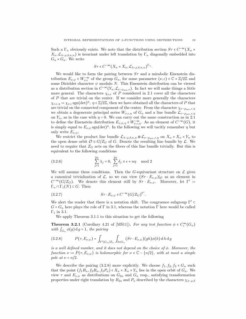
Such a Γn obviously exists. We note that the distribution section Sτ ∈ C−∞(Xn ×Xn,Lλ−ρ,δ,n,n) is invariant under left translation by Γn diagonally embedded intoGn ×Gn. We write

Sτ ∈ C−∞(Xn ×Xn,Lλ−ρ,δ,n,n)Γn .

We would like to form the pairing between Sτ and a mirabolic Eisenstein dis-tribution Eν,ψ ∈ W −∞

ν,ε of the group Gn, for some parameter (ν, ε) ∈ C × Z/2Z andsome Dirichlet character ψ modulo N . This Eisenstein distribution can be viewedas a distribution section in C−∞(Yn,Lν−ρmir,ε). In fact we will make things a littlemore general. The characters χν,ε of P considered in 2.1 cover all the charactersof P that are trivial on the center. If we consider more generally the charactersχν,ε,η ∶= χν,ε sgn(det)η, η ∈ Z/2Z, then we have obtained all the characters of P thatare trivial on the connected component of the center. From the character χν−ρmir,ε,η

we obtain a degenerate principal series Wν,ε,η of Gn and a line bundle Lν−ρmir,ε,η

on Yn, as in the case with η = 0. We can carry out the same construction as in 2.1to define the Eisenstein distribution Eν,ψ,η ∈W −∞

ν,ε,η. As an element of C−∞(G), itis simply equal to Eν,ψ sgn(det)η. In the following we will tacitly remember η butonly write Eν,ψ.

We restrict the product line bundle Lλ−ρ,δ,n,n ⊠ Lν−ρmir,ε,η on Xn ×Xn × Yn tothe open dense orbit O ≅ G/ZG of G. Denote the resulting line bundle by L. Weneed to require that ZG acts on the fibers of this line bundle trivially. But this isequivalent to the following conditions

2n∑j=1

λj = 0,2n∑j=1

δj ≡ ε + nη mod 2(3.2.6)

We will assume these conditions. Then the G-equivariant structure on L givesa canonical trivialization of L, so we can view (Sτ ⋅ Eν,ψ)∣O as an element inC−∞(G/ZG). We denote this element still by Sτ ⋅ Eν,ψ. Moreover, let Γ′ ∶=Γn ∩ Γ1(N) ⊂ G. Then

Sτ ⋅Eν,ψ ∈ C−∞(G/ZG)Γ′ .(3.2.7)

We alert the reader that there is a notation shift. The congruence subgroup Γ′ ⊂G = Gn here plays the role of Γ in 3.1, whereas the notation Γ here would be calledΓ1 in 3.1.

We apply Theorem 3.1.1 to this situation to get the following

Theorem 3.2.1 (Corollary 4.21 of [MS11]). For any test function φ ∈ C∞c (Gn)

with ∫Gn φ(g)d g = 1, the pairing

P (τ,Eν,ψ) = ∫Γ′/Gn/Zn

∫h∈Gn

(Sτ ⋅Eν,ψ)(gh)φ(h)dhd g(3.2.8)

is a well defined number, and it does not depend on the choice of φ. Moreover, thefunction ν ↦ P (τ,Eν,ψ) is holomorphic for ν ∈ C − {n/2}, with at most a simplepole at ν = n/2.

We describe the pairing (3.2.8) more explicitly. We choose f1, f2, f3 ∈ Gn suchthat the point (f1Bn, f2Bn, f3Pn) ∈Xn ×Xn × Yn lies in the open orbit of Gn. Weview τ and Eν,ψ as distributions on G2n and Gn resp., satisfying transformationproperties under right translation by B2n and Pn described by the characters χλ−ρ,δ

20 YIHANG ZHU

and χν,ε resp. Then the distribution Sτ ⋅Eν,ψ, viewed as a distribution on Gn, maybe explicitly expressed as

(Sτ ⋅Eν,ψ)(g) =(3.2.9)

vol((Γ ∩U(Z))/U)−1 ∫(Γ∩U(Z))/U

θ(u)l(u)(τ)(diag(gf1, gf2))Eν,ψ(gf3)du.

Now what is the dependence of (3.2.9) and (3.2.8) on the choice of (fj)? Recallthat in the procedure to form the pairing (3.2.8) that is described above Theorem3.2.1, the choice of the identification O ∼Ð→ Gn/Zn, i.e. the choice of a point insidethe open orbit O, did not affect the pairing. But note that it is with respect to thedistribution sections of the line bundles on X2n and Yn that the pairing in Theorem3.2.1 is canonical. Now if we started with τ and Eν,ψ viewed as distributions on G2nand Gn respectively, and wanted to produce distribution sections of the line bundleson X2n and Yn, we would need to make the choice of identifications G2n/B2n

∼Ð→X2n,Gn/Pn

∼Ð→ Yn. This analysis shows that simultaneous multiplying the fj ’son the left by an element in Gn should not effect the value of (3.2.8), whereasmultiplying the fj ’s individually by elements in Bn and Pn respectively on theright will produce multiplicative factors which are values of χλ−ρ,δ and χν−ρmir,ε.

To be more concrete, note that if (f ′1, f ′2, f ′3) is another such choice, then thereexists f0 ∈ Gn, b1, b2 ∈ Bn, p3 ∈ Pn, such that

f ′j = f0fjbj , j = 1,2, f ′3 = f0f3p3.(3.2.10)

Now left multiplying by f0 results in right translating the expression (3.2.9) by f−10 ,

which will not change the value of (3.2.8) since this translation can be absorbed intoφ. On the other hand, right multiplying by bj , p3 changes the expression (3.2.9) bythe factor χλ−ρ,δ(diag(b1, b2))χν,ε(p3), as can be seen directly.

In the future, we will fix the following choice

f1 = In, f2 = wlong, f3 =⎛⎜⎜⎜⎝

1 1 ⋯ 10⋮ In−10

⎞⎟⎟⎟⎠.(3.2.11)

3.3. Inherited functional equation. The pairings considered in Theorem 3.2.1inherit the functional equation for the mirabolic Eisenstein distributions. Recallthat the functional equation for mirabolic Eisenstein distributions relate Eν,ψ toE−ν,ξ. Of course we may consider the pairing between τ and Eν,ψ that is totallyanalogous to (3.2.8). However it is convenient to insist that the pairing is alwaysbetween a cuspidal automorphic distribution with an un-tilde version of Eisensteindistribution. It turns out that we can transfer the "operation of putting a tilde on E"to some concrete operations on the variable τ , including taking the contragredientτ . Recall that τ was defined and discussed at the end of 1.3. See (1.3.9) and (1.3.10).In the following wlong will be the n × n matrix defined in (1.3.8).


Proposition 3.3.1 (Proposition 4.24 of [MS11]).

P (τ,E−ν,ψ) =

(−1)ε+δn+1+⋯+δ2nN2ν−ν/n−1/2n

∏j=1

Gδn+j+δn+1−j+η(λn+j + λn+1−j + ν/n + 1/2)φ(N)−1×

× ∑a∈Z/NZ

∑ξ∈ (Z/NZ)×

ψ(a)ξ(a)−1P (l (diag(−wlong,wlong)diag(N, In−1,N, In−1)) τ , Eν,ξ) ,

where the pairing on the right hand side is integration over Γ∗/Gn/Zn with

Γ∗ ∶= wlong diag(N, In−1)Γ′ diag(N, In−1)−1wlong, Γ′ = {γ∣γ ∈ Γ′} .

4. Adelization

In this section we put the theory developed in the previous sections into anadelic language. We will use the standard notations about adelic groups. If G is areductive group over Q, the image of G(Q) inside G(A) via the diagonal embeddingwill be denoted by GQ. The component of an adelic point g ∈ G(A) at a place v,resp. away from infinity, will be denoted by gv, resp. gf .

4.1. Adelization of an automorphic distribution. Let G be the reductivegroup GLn over Q. In 1.1 and 1.2, we associated an automorphic distributionτ ∈ (V −∞

λ,δ )Γ to a classical automorphic representation j ∶ V ↪ L2ω(Γ/G(R)). Now

we start with an adelic automorphic representation π ⊂ L2ω(GQ/G(A)), and we want

to construct a family of objects, indexed by gf ∈ G(Af), the members of which areelements of the spaces (V −∞

λ,δ )Γgf , where the Γgf ’s are congruence subgroups ofG(Z) that can vary with gf . We will write this family as

G(A) ∋ g = (g∞, gf)↦ τ(g∞, gf).(4.1.1)

Here τ(⋅, gf) ∈ V −∞λ,δ ⊂ C−∞(G(R)) is a member of the family that we referred to,

and it is a distribution in the variable g∞ ∈ G(R). We have abused notation to viewit as if it were a function in g∞. Using the same notation (4.1.1), we would like τto satisfy the "automorphy property"

τ(γ∞g∞, γfgf) = τ(g∞, gf), for all (g∞, gf) ∈ G(A), (γ∞, γf) ∈ GQ.(4.1.2)

Here we view τ(⋅, γfgf) and τ(⋅, gf) both as elements of the same space C−∞(G(R)).Let π ⊂ L2

ω(GQ/G(A)) be an automorphic representation of G(A). For exampleany cuspidal automorphic representation of central character ω can be realizedinside L2

ω(GQ/G(A)). Here

ω ∶ Z(A) ≅ A× → C×

is a unitary character. By twisting π by a character of G(A) that factors throughdet, we may assume that ω is of finite order. Write ω∞ to be the component of ωat ∞. We decompose π as π =⊗′

v πv. We fix the choice of a vector φA ∈ π that is apure tensor with respect to this decomposition such that its infinity component isa smooth vector for the representation π∞. Let Kf ⊂ G(Z) ⊂ G(Af) be a compactopen subgroup that fixes φA. For any gf ∈ G(Af), the vector π(gf)φA gives rise toan embedding

jπ(gf )φA ∶ π∞ ↪ L2ω∞(Γgf /G(R))(4.1.3)

22 YIHANG ZHU

of the abstract G(R) representation π∞ into L2ω∞(Γgf /G(R)), where Γgf ⊂ G(Z) ⊂

G(R) is the congruence subgroup defined as GQ ∩Kf ⊂ G(Q). Let us constructjπ(gf )φA . Firstly, we define

UφA ⊂ L2ω(GQ/G(A))

to be the subspace spanned by the translates of φA under G(R) ⊂ G(A). Denote theclosure of UφA inside L2

ω(GQ/G(A)) by UφA . Now G(R) acts on UφA , and we mayidentify the G(R) representation π∞ with UφA , since φA is a pure tensor. But anyelement φ inside UφA ⊂ L2

ω(GQ/G(A)), viewed as a function on G(A), is smooth inthe variable in G(R), hence it gives rise to a function

G(R) ∋ g∞ ↦ φ(g∞, gf).(4.1.4)

Moreover the function (4.1.4) lies in L2ω∞(Γgf /G(R)). Thus we obtain a G(R)-

equivariant map

UφA → L2ω∞(Γgf /G(R)).(4.1.5)

The embedding jπ(gf )φA is defined to be the composition of (4.1.5) with the iden-tification π∞

∼Ð→ UφA mentioned above. The notation is justified because jπ(gf )φA

only depends on the vector π(gf)φA.Now as in 1.1, the embedding (4.1.3) gives rise to an element τπ(gf )φA ∈ ((π′∞)−∞)Γgf .

As in (1.2.4) we choose an embedding

(π′∞)−∞ ↪ V −∞λ,δ(4.1.6)

for a suitable principal series Vλ,δ. Now we have finished constructing the family

G(Af) ∋ gf ↦ τπ(gf )φA ∈ (V −∞λ,δ )Γgf .(4.1.7)

We will use the notation (4.1.1). The automorphy property (4.1.2) is easily checked.Moreover, τ satisfies "right-smoothness" for G(Af). Namely, for any k ∈ Kf ⊂G(Af), we have

τ(gk) = τ(g), g ∈ G(A).(4.1.8)

4.2. Adelic Whittaker-Fourier expansion. We study the adelic analogue of theWhittaker-Fourier expansion discussed in 1.3 and 1.4. We will make use of strongapproximation for G = GLn over Q. Recall that this says that GQG(R) is dense inG(A). Note that the analogous statement fails in general if G is a general reductivegroup or if Q is replaced by a number field of class number greater than one.

First we recall the structure of the additive characters on A. Define

Λ∞ ∶ R→ R/Z, x∞ ↦ −x∞ mod 1.Λp ∶ Qp → Z[1/p]/Z, xp ↦ Λp(xp) such that xp −Λp(xp) ∈ Zp.Λ ∶ A→ R/Z, (xv)↦∑

v

Λv(xv).

Then any character of A is of the form

χy ∶ x↦ e(Λ(yx))(4.2.1)

for a unique y ∈ A. Recall that we use the notation e(a) = e2πia. The characterχy is trivial on Q if and only if y ∈ Q ⊂ A. We let ψ+ be the character χ−1. It isthe unique character on A that is trivial on Q and restricts to x∞ ↦ e(x∞) on R.


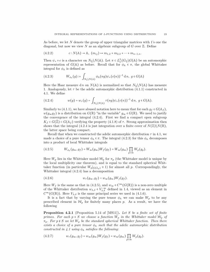
As before, we let N denote the group of upper triangular matrices with 1’s one thediagonal, but now we view N as an algebraic subgroup of G over Z. Define

c ∶ N(A)→ A, (mij)↦m1,2 +m2,3 +⋯ +mn−1,n.(4.2.2)

Then ψ+ ○ c is a character on NQ/N(A). Let π ⊂ L2ω(GQ/G(A) be an automorphic

representation of G(A) as before. Recall that for φA ∈ π, the global Whittakerintegral for φA is defined as

WφA(g) ∶= ∫NQ/N(A)

φA(ng)ψ+(c(n))−1 dn, g ∈ G(A)(4.2.3)

Here the Haar measure dn on N(A) is normalized so that NQ/N(A) has measure1. Analogously, let τ be the adelic automorphic distribution (4.1.1) constructed in4.1. We define

w(g) = wτ(g) = ∫NQ/N(A)

τ(ng)ψ+(c(n))−1 dn, g ∈ G(A).(4.2.4)

Similarly to (4.1.1), we have abused notation here to mean that for each gf ∈ G(Af),w(g∞gf) is a distribution on G(R) "in the variable" g∞ ∈ G(R). We need to justifythe convergence of the integral (4.2.4). First we find a compact open subgroupKf ⊂ G(Z) ⊂ G(Af) verifying the property (4.1.8) of τ . Strong approximation thenshows that the integral (4.2.4 is just integration over a finite cover of N(Z)/N(R),the latter space being compact.

Recall that when we constructed the adelic automorphic distribution τ in 4.1, wemade a choice of a pure tensor φA ∈ π. The integral (4.2.3) for this φA decomposesinto a product of local Whittaker integrals

WφA(g∞, gf) =W∞(g∞)Wf(gf) =W∞(g∞) ∏p<∞

Wp(gp).(4.2.5)

Here Wp lies in the Whittaker model Wp for πp (the Whittaker model is unique bythe local multiplicity one theorem), and is equal to the standard spherical Whit-taker function (in particular Wp∣G(Zp) ≡ 1) for almost all p. Correspondingly, theWhittaker integral (4.2.4) has a decomposition

wτ(g∞, gf) = w∞(g∞)Wf(gf).(4.2.6)

Here Wf is the same as that in (4.2.5), and w∞ ∈ C∞(G(R)) is a non-zero multipleof the Whittaker distribution wλ,δ ∈ V −∞

λ,δ defined in 1.4, viewed as an element inC∞(G(R)). Here Vλ,δ is the same principal series we used in (4.1.6).

It is a fact that by varying the pure tensor φA we can make Wp to be anyprescribed element in Wp for finitely many places p. As a result, we have thefollowing

Proposition 4.2.1 (Proposition 5.14 of [MS11]). Let S be a finite set of finiteprimes. For each p ∈ S we choose a function Wp in the Whittaker model Wp ofπp. For p ∉ S we let Wp be the standard spherical Whittaker function. Then thereexists a choice of a pure tensor φA such that the adelic automorphic distributionconstructed in 4.1 using φA satisfies the following:

wτ(g∞, gf) = w∞(g∞)Wf(gf) = w∞(g∞) ∏p<∞

Wp(gp).(4.2.7)

24 YIHANG ZHU

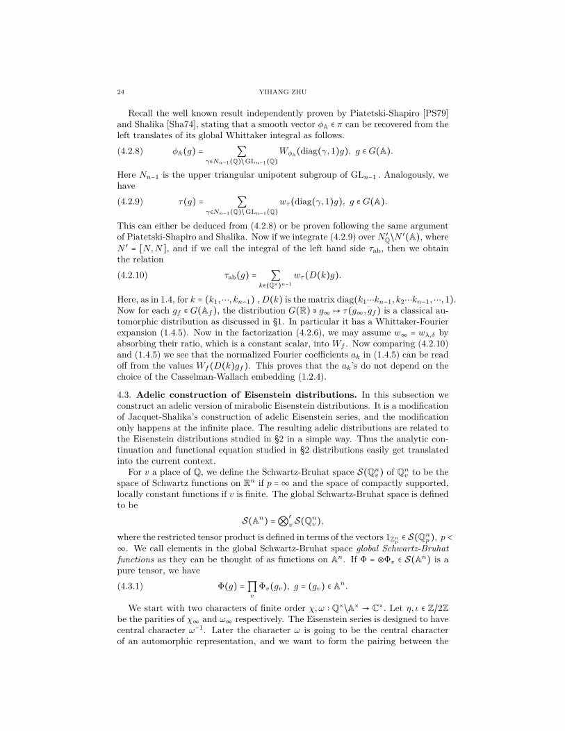
Recall the well known result independently proven by Piatetski-Shapiro [PS79]and Shalika [Sha74], stating that a smooth vector φA ∈ π can be recovered from theleft translates of its global Whittaker integral as follows.

φA(g) = ∑γ∈Nn−1(Q)/GLn−1(Q)

WφA(diag(γ,1)g), g ∈ G(A).(4.2.8)

Here Nn−1 is the upper triangular unipotent subgroup of GLn−1 . Analogously, wehave

τ(g) = ∑γ∈Nn−1(Q)/GLn−1(Q)

wτ(diag(γ,1)g), g ∈ G(A).(4.2.9)

This can either be deduced from (4.2.8) or be proven following the same argumentof Piatetski-Shapiro and Shalika. Now if we integrate (4.2.9) over N ′

Q/N ′(A), whereN ′ = [N,N], and if we call the integral of the left hand side τab, then we obtainthe relation

τab(g) = ∑k∈(Q×)n−1

wτ(D(k)g).(4.2.10)

Here, as in 1.4, for k = (k1,⋯, kn−1) ,D(k) is the matrix diag(k1⋯kn−1, k2⋯kn−1,⋯,1).Now for each gf ∈ G(Af), the distribution G(R) ∋ g∞ ↦ τ(g∞, gf) is a classical au-tomorphic distribution as discussed in §1. In particular it has a Whittaker-Fourierexpansion (1.4.5). Now in the factorization (4.2.6), we may assume w∞ = wλ,δ byabsorbing their ratio, which is a constant scalar, into Wf . Now comparing (4.2.10)and (1.4.5) we see that the normalized Fourier coefficients ak in (1.4.5) can be readoff from the values Wf(D(k)gf). This proves that the ak’s do not depend on thechoice of the Casselman-Wallach embedding (1.2.4).

4.3. Adelic construction of Eisenstein distributions. In this subsection weconstruct an adelic version of mirabolic Eisenstein distributions. It is a modificationof Jacquet-Shalika’s construction of adelic Eisenstein series, and the modificationonly happens at the infinite place. The resulting adelic distributions are related tothe Eisenstein distributions studied in §2 in a simple way. Thus the analytic con-tinuation and functional equation studied in §2 distributions easily get translatedinto the current context.

For v a place of Q, we define the Schwartz-Bruhat space S(Qnv ) of Qnv to be thespace of Schwartz functions on Rn if p =∞ and the space of compactly supported,locally constant functions if v is finite. The global Schwartz-Bruhat space is definedto be

S(An) =⊗′

v S(Qnv ),

where the restricted tensor product is defined in terms of the vectors 1Znp ∈ S(Qnp), p <

∞. We call elements in the global Schwartz-Bruhat space global Schwartz-Bruhatfunctions as they can be thought of as functions on An. If Φ = ⊗Φv ∈ S(An) is apure tensor, we have

Φ(g) =∏v

Φv(gv), g = (gv) ∈ An.(4.3.1)

We start with two characters of finite order χ,ω ∶ Q×/A× → C×. Let η, ι ∈ Z/2Zbe the parities of χ∞ and ω∞ respectively. The Eisenstein series is designed to havecentral character ω−1. Later the character ω is going to be the central characterof an automorphic representation, and we want to form the pairing between the


adelic distribution of that automorphic representation and the adelic Eisensteindistribution to be constructed in the following. We allow the character χ in thetheory to make the theory applicable not only to the untwisted L-functions, butalso to the twisted ones. Let P ′ be the group of upper triangular (n − 1,1)-blockmatrices, thought of as an algebraic subgroup of G. Then P ′ = wlongPwlong, wherethe group of R points of P was denoted by P in 2.1. For any global Schwartz-Bruhatfunction Φ, Jacquet-Shalika define the following integral

I(g, s) = χ(det g)−1 ∣det g∣s ∫A×

Φ(entg) ∣t∣ns χ(t)−nω(t)d∗ t, g ∈ G(A), s ∈ C.(4.3.2)

Here en is the row vector (0,⋯,0,1) viewed as an element in An, and ∣⋅∣ means theproduct of the local normalized absolute values defined on Q×/A×. The integralI(g, s) is designed to satisfy the following transformation property: For

p′ = ( B ∗a

) ∈ P ′(A),B ∈ GLn−1(A), a ∈ A×,

since entp′g = enatg, we have

I(p′g, s) = χ(a)nω(a)−1 ∣a∣−ns χ(detp′)−1 ∣detp′∣s I(g, s).(4.3.3)

If Φ =∏Φv is a pure tensor, then the integral I(g, s) factors into a product of localintegrals

I(g, s) =∏v

Iv(gv, s) = I∞(g∞, s)If(gf , s), g = (gv) ∈ G(A),(4.3.4)

where

Iv(gv, s) = χv(det gv)−1 ∣det gv ∣s ∫Q×v

Φv(entgv) ∣t∣ns χv(t)−nωv(t)d∗ t,(4.3.5)

and in particular

I∞(g∞, s) = sgn(det g∞)η ∣det g∞∣s ∫R×

Φ∞(entg∞) ∣t∣ns sgn(t)nη+ι d∗ t.(4.3.6)

Jacquet-Shalika then consider the Eisenstein series defined as

E(g, s) = ∑γ∈P ′

Q/GQ

I(γg, s).(4.3.7)

Here it is easy, at least formally, to see that if γ ∈ P ′Q, then I(γg, s) = I(g, s). By

design this series satisfies the automorphy property

E(γg, s) = E(g, s), γ ∈ GQ.(4.3.8)

The adelic construction of the Eisenstein distribution is the same as Jacquet-Shalika’s construction, except that at the place ∞ the Schwartz function Φ∞ isreplaced by a distribution. In the following we will add subscripts JS and D todistinguish between the case of Jacquet-Shalika and the case of distribution.

Suppose ΦD,∞ ∈ C−∞(Rn) is a distribution on Rn. Let Φp ∈ S(Qnp), p <∞, andsuppose for almost all p, Φp is the characteristic function of Znp . Then we can form

26 YIHANG ZHU

ΦD, ID(g, s) and ED(g, s) using the same formulas as (4.3.1), (4.3.2) and (4.3.7).

ΦD(g) = ΦD,∞(g∞) ∏p<∞

Φp(gp),(4.3.9)

ID(g, s) = χ(det g)−1 ∣det g∣s ∫A×

ΦD(entg) ∣t∣ns χ(t)−nω(t)d∗ t,(4.3.10)

ED(g, s) = ∑γ∈P ′

Q/GQ

ID(γg, s).(4.3.11)

Formally ED(g, s) satisfies the following property of automorphy:

ED(γg, s) = ED(g, s), γ ∈ GQ.(4.3.12)

It also satisfies right G(Af)-smoothness, inheriting from the property of Φf . Thismeans: there exists an open compact subgroup Kf ⊂ G(Af), such that

ED(gk, s) = ED(g, s), k ∈Kf .(4.3.13)

Of course now the integral ID(g, s) has its archimedean factor ID,∞(g∞, s) being adistribution in the variable g∞. This integral ID,∞(g∞, s) is related to an integralof Jacquet-Shalika’s type in the following way. Let φ ∈ C∞

c (G(R)). Let

ΦJS,∞(v) ∶= ∫G(R)

ΦD,∞(vh)φ(h) sgn(deth)η ∣deth∣s dh, v ∈ Rn.(4.3.14)

Then the resulting local integrals ID,∞ and IJS,∞ defined using ΦD,∞ and ΦJS,∞are related by

IJS,∞(g∞, s) = ∫G(R)

ID,∞(g∞h, s)φ(h)dh.(4.3.15)

To make a link to the Eisenstein distribution discussed in §2, we compute ID(g, s)for a specific choice of the Φv’s. We choose ΦD,∞ to be δe1 , that it, Dirac’s deltafunction supported at the point e1 = (1,0,⋯,0) ∈ Rn. For p < ∞, we choose Φp tobe the characteristic function of the set en + pNpZp, where Np ∈ Z≥0 and is zero foralmost all p. Let N =∏p pNp . We assume N is large enough such that there existsa Dirichlet character ψ modulo N , whose adelization ψA ∶ Q×/A× → C× is equal tothe finite order character χnω−1.

We compute ID,∞(g∞, s). Let ε = nη + ι ∈ Z/2Z, so that ψ(−1) = (−1)ε. Letν = n(s − 1/2). Then using (4.3.6) one sees that ID,∞(g∞, s) is a constant multipleof the distribution

δ∞ ⋅ sgn(det)η ∈W −∞ν,ε,η =W −∞

ν,ε ⊗ sgn(det)η,(4.3.16)

where δ∞ ∈W −∞ν,ε was considered in 2.1. From now on we will use δ∞ to denote the

element 4.3.16.For a prime p < ∞, we first use the locally-at-p version of the transformation

law (4.3.4) to reduce the computation of Ip(gp, s) in general to the case wheregp ∈ G(Zp). In this case, let v be the last row of gp, then v has an entry in Z×p . Wehave

Ip(gp, s) = χp(det gp)−1 ∣det gp∣s ∫t ∈ Qp×

tv ∈ en + pNpZnp

∣t∣ns ψp(t)−1 d∗ t.(4.3.17)


If Np = 0, the integral in (4.3.17) is equal to

∫t ∈ Qp×

0 < ∣t∣ ≤ 1

∣t∣ns ψp(t)−1 d∗ t = (1 − ψ(p)p−ns)−1.

The equality here is due to Tate’s construction of Dirichlet’s L-functions, notingthat ψ is unramified at p.

If Np > 1, the integral in (4.3.17) is zero unless

v ≡ (0,0,⋯,0,1) mod pNp ,

in which case it is equal to a constant times ψp(vn), where vn is the last entry ofv. In summary, for gf ∈ G(Z) ⊂ G(Af), we have

ID(g∞, gf , s) = Cδ∞(g∞)χf(det gf)−1 ∣det gf ∣s ψAf ((gf)nn)L(ns,ψ)1K0(N)(gf),(4.3.18)

where C is a constant, and 1K0(N) is the characteristic function of the subgroupK0(N) = {g ∈ G(Z)∣gin ≡ 0 mod N, 1 ≤ i ≤ n − 1} ⊂ G(Af). In particular, for γ ∈G(Z) ⊂ GQ, g∞ ∈ G(R), writing γ = (γ∞, γf), we have

ID(γg∞, s) = Cδ∞(γ∞g∞)χ∞(detγ∞) ∣detγ∞∣−s ψ∞((γ∞)nn)ψ(γnn)L(ns,ψ)1Γ0(N)(γ)(4.3.19)

= Cδ∞(γ∞g∞) sgn(detγ)η sgn(γnn)εψ(γnn)L(ns,ψ)1Γ0(N)(γ)= Cl(γ∞)(δ∞)(g∞)ψ(γnn)L(ns,ψ)1Γ0(N)(γ).

We see that if we sum (4.3.19) over γ ∈ P ′(Z)/G(Z), we get exactly the expression(2.1.4) defining the classical Eisenstein distribution. Observe that the inclusion mapG(Z) ↪ G(Q) induces a bijection between P ′(Z)/G(Z) and P ′(Q)/P (Q). Hencewe have

ED(g, s) = Eν,ψ(g), g ∈ G(R) ⊂ G(A).(4.3.20)

For general g ∈ G(A), we can also equate E(g, s) with some E(g′, s), g′ ∈ G(R),using strong approximation, in view of (4.3.12) and (4.3.13). (In fact we can takeKf =K0(N).)

We may generalize our choice of the data Φv a bit. Define SD(Rn) ⊂ C−∞(Rn) tobe the vector space spanned (algebraically) by delta functions at points in Rn. Thenfor any Φ ∈ SD(Rn)⊗⊗′

p S(Qnp), the Eisenstein distribution (4.3.11) defined using Φcan be obtained from the special kind of Eisenstein distributions discussed above. Infact, replacing Φ(v) by Φ(vh), h ∈ G(A) has the effect of right translating ED(g, s)by h. Also S(Af) is spanned by Φf(v + ⋅), where v runs over Anf and Φf runs overthe special choices of Φf discussed above. As a result, for any fixed gf ∈ G(Af),the defining series (4.3.11) all converge in the strong distribution topology in theg∞ variable for Rs > 1, and have meromorphic continuation to s ∈ C, with at mosta simple pole at s = 1 which occurs when ψ is nontrivial.

4.4. Adelization of the automorphic pairing. We generalize the automorphicpairing discussed in 3.2 to an adelic version. We now denote by U the algebraic

28 YIHANG ZHU

subgroup of GL2n whose group real points was denoted by U in 3.2. We extendthe character θ defined in (3.2.4) to an adelic character:

θ ∶ UQ/U(A)→ C×, ( In AIn

)↦ ψ+(trA).(4.4.1)

Let du be the Haar measure on U(A) that gives UQ/U(A) measure 1. Let G denoteGLn and let Z denote its center. Let f1, f2, f3 ∈ G(R) be such that the point(f1Bn, f2Bn, f3Pn) in the product of flag varieties Xn ×Xn ×Yn = Gn(R)/Bn(R)×Gn(R)/Bn(R) × Gn(R)/Pn(R) lies in the open orbit under the diagonal G(R) =Gn(R) action. Here the groups Gn(R),Bn(R), Pn(R) were the real Lie groupsdenoted by Gn,Bn, Pn in 3.2. For definiteness we will take the choice (3.2.11). Letφ ∈ C∞

c (G(R)) with total integral 1. Let π be a cuspidal automorphic representationof GL2n(A), with corresponding adelic automorphic distribution τ , as in 4.1, andlet E(g, s) be an adelic Eisenstein distribution considered in 4.3, for the groupG = GLn. We assume that the character ω used in the construction in 4.3 is thesame as the central character of τ , both viewed as characters on A×. The adelicautomorphic pairing between τ and E is defined as

P (τ,E(⋅, s)) ∶=

(4.4.2)

∫Z(A)GQ/G(A)

∫G(R)

[∫UQ/U(A)

τ(udiag(ghf1, ghf2))θ(u)du]E(ghf3, s)φ(h)dhd g.

Let us explain the reason why this integral makes sense by relating it to the classicalautomorphic pairing in Theorem 3.2.1. The basic idea is that both τ(g) and E(g, s)satisfy the property of automorphy (i.e. left invariance under GQ for the respectivegroups G) and right smoothness under G(Af) for the respective groups G. Thesesproperties allow us to use strong approximation to reduce the integrals consideredhere to those considered in 3.2. Firstly, for the same reason as in the justificationfor the convergence of (4.2.4), the integration in 4.4.2 in the bracket is just anintegration over a finite cover of the compact space U(Z)/U(R), so for each fixedgf and hf it gives rise to a distribution in the variable g∞h∞. Moreover, this "adelicdistribution" is left invariant under GQ, inheriting the automorphy property (4.1.2).It is also invariant under Z(A), since τ(g) and E(gs) have central characters ωand ω−1 respectively. These two kinds of invariance remain unchanged by the dhintegral. Now the dh integral gives us, for each gf ∈ G(Af), a distribution in thevariable g∞ ∈ G(R), which is of the same type as the integrand of the d g integralin Theorem 3.2.1. (See the discussion after Theorem 3.2.1.) Now the convergenceof the d g integral in (4.4.2), and the independence of the choice of φ, both followfrom Theorem 3.2.1.

The pairing (4.4.2), viewed as a function in s, naturally inherits the analyticcontinuation and functional equation from its classical counterpart. We state thefunctional equation as follows. We choose parameters (λ, δ) ∈ C2n × (Z/2Z)2n tohave a Casselman embedding for π′∞ as in (4.1.6). We remind the reader that theparity ι of ω and the parameter δ have to satisfy

ι ≡ δ1 +⋯ + δ2n mod 2.(4.4.3)


Recall that when we related the adelic Eisenstein distribution E(g, s) to a classicalone Eν,ψ ∈Wν,ε, we had relations

ψ(−1) = (−1)ε, ε ≡ nη + ι mod 2.(4.4.4)

We see that the relations (4.4.3) and (4.4.4) do recover the condition (3.2.6). Weassume the data Φ = Φ∞Φf chosen to define E has Φ∞ = δe1 . Then the functionalequation is

P (τ,E(1 − s)) = N2ns−s−nn

∏j=1

Gδn+j+δn+1−j+η(s + λn+j + λn+1−j)P (τ ′,E′(s)).

(4.4.5)

Here τ ′ is a translate of τ by an element in GL2n,Q which is unramified at theprimes where τ and E(s) are. (Here unramification at a prime p means beingright invariant under G(Zp) for the respective group G. It can be seen that E(s) isunramified at p if Φ = 1Znp , i.e. if Φ is unramified at p. The adelic distribution E′ is amirabolic Eisenstein distribution defined using a linear combination of different Φ’s,each having Φ∞ = δe1 . In particular, if we assume that τ is anywhere unramified, ωis trivial, and the data Φ used to define E(s) is unramified, i.e. equal to δe1 ⋅ 1Zn ,then the functional equation simplifies to

P (τ,E(1 − s)) = (−1)δ1+⋯+δnn

∏j=1

Gδn+j+δn+1−j(s + λn+j + λn+1−j)P (τ , E(s)).(4.4.6)

5. The exterior square L-function

In this section we study the exterior square L-function L(s, π,Ext2⊗χ) for acuspidal automorphic representation π of GL2n(A), where χ is a Dirichlet character.Recall that for a finite prime p at which both π and χ are unramified, the localEuler factor of L(s, π,Ext2⊗χ) at p is defined to be

Lp(s, π,Ext2⊗χ) = ∏1≤j<k≤2n

(1 − αp,jαp,kχ(p)p−s)−1,(5.0.1)

where the αp,j ’s are the principal series parameters for the unramified representationπp.

Let τ be an adelic automorphic distribution associated to π. We compute the au-tomorphic pairing (4.4.2) and relate it to the partial Euler products LS(s, π,Ext2⊗χ).The functional equation and full holomorphy of the (partial) L-functions would thenfollow from the analytic properties of the pairing (4.4.2). Throughout this sectionit will often be tacitly assumed that Rs is large enough, since this already sufficesif one wants to compare any two meromorphic functions in the variable s.

5.1. Overview. The construction of the automorphic pairing P (τ,E(s)) in 4.4 ismodeled on the analogous integral considered by Jacquet-Shalika in their theory ofintegral representation of exterior square L-functions [JS90]. Jacquet-Shalika’s in-tegral integrates the product of an adelic automorphic form and an adelic mirabolicEisenstein series. Thus the automorphic pairing (4.4.2) is a distribution analogueof Jacquet-Shalika’s integral, where the automorphic form and the Eisenstein seriesare replaced by their respective distribution counterparts. Jacquet-Shalika com-pute the unfolding of their integral, relating the integral to the exterior squareL-function of π. The automorphic pairing P (τ,E(s)) unfolds in a similar way. In

30 YIHANG ZHU

fact, following [MS12a], we will reduce the unfolding of P (τ,E(s)) to the case ofJacquet-Shalika, by relating it to an integral of Jacquet-Shalika type.

To be more specific, for each place v, Jacquet-Shalika define a function Ψv(s,Wv,Φv)in s, whereWv is in the Whittaker model of πv and Φv ∈ S(Qnv ) is a Schwartz-Bruhatfunction at v. They show that their integral pairing between the automorphic formand the mirabolic Eisenstein series with parameter s unfolds to be a product ofthese functions Ψv. When p <∞ is an unramified prime (i.e. such that πp, χp andΦp are all unramified1), Jacquet-Shalika compute

Ψp(s,Wp,Φp) = Lp(s, π,Ext2⊗χ).(5.1.1)Thus their integral is related to the exterior square L-function. However the fac-tor Ψ∞(s,W∞,Φ∞) in Jacquet-Shalika’s setting is very difficult to compute, thusJacquet-Shalika’s representation of the L-function is not sufficient to prove the fullholomorphy result which the method of Miller-Schmid can prove. As we will de-scribe, in [MS12a], Miller-Schmid show that their automorphic pairing (4.4.2) canbe related to a certain Jacquet-Shalika type integral. As a result the automorphicpairing is equal to a product of Jacquet-Shalika’s Ψv’s. Then by a sort of reverseprocedure at the place ∞, we obtain the equality

P (τ,E(s)) = Ψ∞(s,wλ,δ) × ∏p<∞

Ψp(s,Wp,Φp),(5.1.2)

where the term Ψ∞(s,wλ,δ) is explicitly defined, and is the analogue of Jacquet-Shalika’s Ψ∞(s,W∞,Φ∞). The details of the argument will be given in 5.2.

Then the remaining task is to calculate the term Ψ∞(s,wλ,δ). The huge ad-vantage of the method of Miller-Schmid is that this term can actually be com-pletely calculated in terms of the functions Gδ, unlike the term Ψ∞(s,W∞,Φ∞)in Jacquet-Shalika theory. We will carry out the calculation of Ψ∞(s,wλ,δ) in 5.3.The conclusion of the calculation will be

Proposition 5.1.1. We haveΨ∞(s,wλ,δ) = κG(s),(5.1.3)

whereκ = (−1)(n+1)η+∑nj=2 δj+∑

n−1j=1 δ2j ,(5.1.4)

G(s) = ∏1≤i<j≤2n,i+j≤2n

Gδi+δj+η(s − λi − λj).(5.1.5)

In particular, let S a finite set of finite primes containing all the ramified primes.Then for Rs sufficiently large, the automorphic pairing (4.4.2) is equal to

P (τ,E(s)) = κG(s)LS∪{∞}(s, π,Ext2⊗χ)∏p∈S

Ψp(s,Wp,Φp).(5.1.6)

From Proposition 5.1.1, we will deduce the functional equation and full holomor-phy of the (partial) L-function in 5.4.

We ask the reader to notice the following discrepancy of notations between ourexposition and [MS12a]. In loc. cit. U means our group Un = the group of upper

triangular unipotent n × n matrices, whereas the group Un,n = ( In Mn×n

In) ⊂

GL2n in loc. cit. is denoted by U in our notation.

1Recall that saying Φp is unramified means that it is equal to 1Znp .


5.2. Unfolding of the automorphic pairing. Let χ ∶ Q×/A× → C× be a char-acter of finite order. This character will appear in the definition of the Eisensteindistribution as in 4.3, as well as in the L-function L(s, π,Ext2⊗χ). Let v be a placeof Q, and let Φv ∈ S(Qnv ) be a Schwartz-Bruhat function. Let Wv be an element ofthe Whittaker modelWv of πv. Let σ ∈ GL2n,Q be the "card shuffle matrix" definedas

σ = E11 +E32 +E53 +⋯ +E2n−1,n +E2,n+1 +E4,n+2 +⋯ +E2n,2n.(5.2.1)

Let G = GLn, N ⊂ G be the subgroup of unipotent upper triangular matrices,U ⊂ GL2n as before, and L0 ⊂ U be the subgroup of matrices whose top right n×nblock is strictly lower triangular. Define

Ψv(s,Wv,Φv) ∶= ∫N(Qv)/G(Qv)

∫L0(Qv)

Wv(σl diag(g, g))Φv(eng) ∣det g∣s χ(det g)−1 d l d g.(5.2.2)

Jacquet-Shalika show that their integral pairing equals the product of these Ψv’sover all the places v.

Now we will follow [MS12a] to show the unfolding (5.1.2) of the automorphicpairing P (τ,E(s)) by reducing to the case of Jacquet-Shalika. First let us denotethe integrand for the d g integral in (4.4.2) by F (g).

F (g) = ∫G(R)

[∫UQ/U(A)

τ(udiag(ghf1, ghf2))θ(u)du]E(ghf3, s)φ(h)dh, g ∈ G(A)

(5.2.3)

P (τ,E(s)) = ∫Z(A)GQ/G(A)

F (g)d g.(5.2.4)

We can introduce an extra smoothing over U(R) to get a different expression forF (g). Let φU ∈ C∞

c (U(R)) be any function with total integral one on U(R). DenoteθU ∶= φU θ. Consider

Φ(g2n, gn) ∶= ∫Gn(R)

∫U(R)

τ(g2nudiag(hf1, hf2))E(gnhf3, s)φθ(u)duφ(h)dh,(5.2.5)

for gn ∈ Gn(R), g2n ∈ G2n(R). The function Φ is a smooth function on the groupG2n(R) ×Gn(R), and we have

F (g) = ∫UQ/U(A)

Φ(udiag(g, g), g)θ(u)du(5.2.6)

We next argue that for a suitable choice of φ and φθ, the function Φ(g2n, gn) factorsas a product of a cusp form in the variable g2n, and a mirabolic Eisenstein series inthe sense of Jacquet-Shalika in the variable gn. In fact, the diagonal Gn(R) actionon Xn×Xn×Yn induces a local diffeomorphism between a neighborhood of identityin Gn(R)/Zn(R) and a neighborhood of the point (f1, f2, f3) in Xn ×Xn ×Yn. Westart with smooth compactly supported functions φj on Xn,Xn and Yn respectivelywith their supports concentrated near the points fj , j = 1,2,3. Then under the localdiffeomorphism mentioned above, the functions φj correspond to a smooth functionφ ∈ C∞

c (Gn(R)/Zn(R). Notice that in the definition (5.2.5), the inner integral gives

32 YIHANG ZHU

rise to a distribution on Gn(R) that is invariant under Zn(R), so the operation

∫Gn(R)

⋯φ(h)dh(5.2.7)

with some φ ∈ C∞c (Gn(R)) can be replaced by the operation

∫Gn(R)/Zn(R)

⋯φ(h)dh(5.2.8)

with some φ ∈ C∞c (Gn(R)/Zn(R)), and the value of Φ(g2n, gn) will only be changed

by a scalar multiple. But if we use (5.2.8) to compute Φ(g2n, gn), with the choiceof φ ∈ C∞

c (Gn(R)) constructed before, we see that Φ(g2n, gn) becomes a productof two factors: one factor is the smoothing of τ over an open set of X2n, and theother factor is the smoothing of E(s) over an open set of Yn. By assuming thatthe supports of the φj ’s and of φU are small enough, we may assume that theabove mentioned open sets of X2n and Yn are contained inside the translated openSchubert cells diag(f1, f2)N2n(R) ⊂ X2n and f3Un(R) ⊂ Yn respectively. Then wehave

Φ(g2n, gn) = Φcusp(g2n)ΦEis(gn),(5.2.9)

Φcusp(g2n) = ∫n′∈N2n(R)

τ(g2n diag(f1, f2)n′)φ′(n′)dn′(5.2.10)

ΦEis(gn)∫U(R)

E(gnf3u, s)φ′′(u)du,(5.2.11)

where both φ′ ∈ C∞c (N2n(R)) and φ′′ ∈ C∞

c (U(R)) have their supports concentratednear the identity. This is the factorization of Φ(g2n, gn) into the product of a cuspform and a mirabolic Eisenstein series which we set out to show.

With the factorization (5.2.9) and formulas (5.2.4), (5.2.6), the pairing P (τ,E(s))becomes equal to an integral pairing considered by Jacquet-Shalika. Now accordingto Jacquet-Shalika [JS90], the pairing P (τ,E(s)) is equal to the following product:

P (τ,E(s)) =∏v

Ψv(s,WJS,v,ΦJS,v),(5.2.12)

where v runs over all the places, WJS,v is the local Whittaker integral of the cuspform Φcusp, and ∏v ΦJS,v ∈ S(An) is the Schwartz-Bruhat function used to definethe Eisenstein series ΦEis. Now suppose that the automorphic distribution τ has itsglobal Whittaker integral as in (4.2.7), and suppose that the Eisenstein distributionE(s) is built from the data ΦD = ΦD,∞∏pΦp, with ΦD,∞ = δe1 . Then we have

WJS,p =Wp, ΦJS,p = Φp, p <∞(5.2.13)

WJS,∞(g2n) = ∫N2n(R)

wλ,δ(g2n diag(f1, f2)n′)φ′(n′)dn′(5.2.14)

ΦJS,∞(v) = ∫Un(R)

δe1(vf3u)φ′′(u)du, v ∈ Rn.(5.2.15)

In particular, we plug in the relations (5.2.14) and (5.2.15) into the definition (5.2.2)of Ψ∞, and get

Ψ∞(s,WJS,∞,ΦJS,∞)(5.2.16)

= ∫N(R)/G(R)

∫L0(R)

[∫N2n(R)

wλ,δ(σl diag(gf1, gf2)n′)φ′(n′)dn′]×

× [∫Un(R)

δe1(engf3u)φ′′(u)du] ∣det g∣s sgn(det g)η d l d g.


Then a procedure similar to the reverse of the factorization of Φ(g2n, gn) showsthat this last integral is equal to, up to a scalar,

Ψ∞(s,wλ,δ) ∶=(5.2.17)

∫Z(R)N(R)/G(R)

∫G(R)

∫L0(R)

wλ,δ(σl diag(ghf1, ghf2))I∞(ghf3, s)φ(h)d l dhd g.

Here I∞(g, s) is the integral ID,∞(g, s) considered in 4.3, with the choice ΦD,∞ = δe1 .We also have the following expression, which is a direct one-step computation fromthe definition (5.2.2):

Ψ∞(s,wλ) = Ψ∞(s,WJS,∞,ΦJS,∞) =(5.2.18)

= ∫Z(R)N(R)/G(R)

∫L0(R)

WJS,∞(σl diag(g, g))IJS,∞(g, s)d l d g.

Here IJS,∞ is the integral used to define the Eisenstein series ΦEis(gn) as in 4.3,and its relation to I∞ is

IJS,∞(gn, s) = ∫Un(R)

I∞(gnf3u, s)φ′′(u)du.(5.2.19)

As remarked in [MS12a] §3, the integral in (5.2.17) can be thought of as a "localpairing" between the classical distributions wλ,δ and I∞, and (5.2.18) renders it asa "local pairing" between the smooth functions WJS,∞ and IJS,∞. At this point wehave proven the following

Proposition 5.2.1.

P (τ,E(s)) = Ψ∞(s,wλ,δ) × ∏p<∞

Ψp(s,Wp,Φp).(5.2.20)

We remark that although when deducing (5.2.20) we made some special assump-tions on the choice of the function φ, both sides of (5.2.20) do not depend on thechoice of φ. Our next task is to calculate the "local pairing" Ψ∞(s,wλ,δ) explicitly.

5.3. Calculation of Ψ∞(s,wλ,δ). We now calculate the "local pairing" Ψ∞(s,wλ,δ)defined in (5.2.17) or (5.2.18). Recall that Ψ∞(s,wλ,δ) only depends on the threeparameters s, λ, δ, (and the implicit parameter η), but not any longer on the au-tomorphic representation π. We will always assume Rs is sufficiently large in ourcalculation. Moreover, for the sole purpose of the brevity of the exposition, we willdisregard the various sign changes in the process of the calculation. These signchanges could all have been explicitly kept track of, and the interested reader caneither check each step herself/himself or refer to [MS12a]. In the exposition wewill not emphasize that the equality is up to a sign. We will denote the smoothWhittaker function WJS,∞ from the previous subsections simply by W∞.

We denote by wk the k × k matrix wlong. Let

h0 =

⎛⎜⎜⎜⎜⎜⎝

0 1 1 ⋯ 10 1 ⋯ ⋮

⋱ ⋱ ⋮0 1

−1 1 1 ⋯ 1

⎞⎟⎟⎟⎟⎟⎠

.(5.3.1)

34 YIHANG ZHU

In the integral (5.2.17) we perform a right translation of the variable h by h0, thenthe value of the integral remains the same up to a sign, and the effect is equivalentto replacing the old choice of f1, f2, f3 in (3.2.11) by the new choice

f1 =⎛⎜⎜⎜⎝

1In−1 ⋮

11

⎞⎟⎟⎟⎠, f2 = ( wn−1

1 ) , f3 = wn.(5.3.2)

The integrand of the d g integral in (5.2.18) is smooth, so we may replace the inte-gration domain Z(R)N(R)/G(R) by a dense open subset of it. The set Bn(R)1 ∶={g ∈ Bn(R)∣gnn = 1} can be viewed as such a dense open subset of Z(R)N(R)/G(R).Let

B′(R) ∶= {C = diag(b,1)∣b ∈ Bn−1(R)} , Q(R) ∶=

⎧⎪⎪⎪⎪⎪⎨⎪⎪⎪⎪⎪⎩

⎛⎜⎜⎜⎝

1⋱

1∗ ⋯ ∗ 1

⎞⎟⎟⎟⎠

⎫⎪⎪⎪⎪⎪⎬⎪⎪⎪⎪⎪⎭

.(5.3.3)

Then we have a diffeomorphism

B′(R) ×Q(R) ∼Ð→ Bn(R)1, (C, q)↦ Cq.(5.3.4)

The Haar measure d g restricted to B′(R) ×Q(R) is equal to

(n−1∏j=1

∣cj,j ∣j−(n+1)/2) ∣detC ∣−(n+1)/2 ∏1≤j≤i<n

d ci,j d q,(5.3.5)

where the ci,j ’s are the entries of the matrix C ∈ B′(R), the measure d ci,j is theLebesgue measure on the ci,j-line R, and d q is the Lebesgue measure on Q(R) ≅Rn−1. We will abbreviate the expression (5.3.5) as

∣C−ρ∣ ∣detC ∣−(n+1)/2 dC d q.(5.3.6)Summarizing what we have done, we have

Ψ∞(s,wλ) =(5.3.7)

= ∫Rn−

∫Q(R)

∫L0(R)

W∞(σl diag(Cq,Cq))IJS,∞(Cq, s)d l ∣C−ρ∣ ∣detC ∣−(n+1)/2 d q dC

= ∫Rn−

∫L0(R)

∫Q(R)

W∞(σl diag(Cq,Cq))IJS,∞(Cq, s)d q d l ∣C−ρ∣ ∣detC ∣−(n+1)/2 dC

where n− ∶= n(n − 1)/2. We compute the d q integral in the last line by expandingthe definition (5.2.19):

∫Q(R)

W∞(σl diag(Cq,Cq))IJS,∞(Cq, s)d q

=∫Q(R)

∫Un(R)

W∞(σl diag(Cq,Cq))I∞(Cqf3u, s)φ′′(u)dud q.(5.3.8)

Recall that f3 = wn. We haveI∞(Cqf3u, s) = ∣detC ∣s sgn(detC)ηI∞(qf3u, s)(5.3.9)

= ∣detC ∣s sgn(detC)η sgn(detwn)ηδe(qwnuwn).


As a result, (5.3.8) equals to

∫Q(R)

W∞(σl diag(Cq,Cq))φ′′(wnq−1wn)d q ∣detC ∣s sgn(detC)η.(5.3.10)

To compute the d l integral in the last line of (5.3.7), we introduce coordinates toL0(R) as follows.

L0(R) ∋ l = ( In ZIn

) , Z =⎛⎜⎜⎜⎝

0z1,1 0⋮ ⋱ ⋱

zn−1,1 ⋯ zn−1,n−1 0

⎞⎟⎟⎟⎠.(5.3.11)

Then the Haar measure on L0(R) is given byd l = dZ ∶= ∏

1≤j≤i<nd zi,j ,(5.3.12)

and satisfiesd(ZC−1) = ∣C−ρ∣ ∣detC ∣(1−n)/2 dZ.(5.3.13)

We plug (5.3.8) and (5.3.12) into the last line of (5.3.7), and get

Ψ∞(s,wλ,δ) = ∫Rn−∫Q(R)

∫Rn−

W∞ (σ ( Cq ZqCq

))×(5.3.14)

×φ′′(wnq−1wn) ∣C−2ρ∣ ∣detC ∣s−n sgn(detC)η dZ d q dC.

We remind the reader that in (5.3.14), the term W∞ implicitly contains φ′. Recallthat when the supports of φ′ ∈ C∞

c (N2n(R)) and φ′′ ∈ C∞c (Un(R)) are concen-

trated near the identities enough, the two functions together produce a functionφ ∈ C∞

c (G(R)/Z(R), and φ′ and φ′′ should satisfy the constraint that the totalintegral of φ is one. Notice that for any φ′, φ′′, if their supports shrink to {e},then the product of their respective total integrals tends to the total integral of thecorresponding function φ. The reason for that is that at identities, the charactersdefining the relevant line bundles on the flag varieties both take the value 1. Thisimplies that, if we take {φ′} ,{φ′′} to be two sequences of approximate identities,with their supports tending to {e}, then the expression on the right hand side of(5.3.14) tends to Ψ∞(s,wλ,δ), when both of the supports of φ′ and φ′′ are simulta-neously arbitrarily small. However, in view of the smoothness of the function W∞,we can first fix a φ′, replace φ′′ by δe, and then take the limit in φ′, and we willstill get the number Ψ∞(s,wλ,δ). Therefore, for a family {φ′} ⊂ C∞

c (N2n(R)) ofapproximate identities surrounding e, we have

∫Rn(n−1)

W∞ (σ ( C ZC

))dµÐ→ Ψ∞(s,wλ,δ),(5.3.15)

wheredµ = ∣C−2ρ∣ ∣detC ∣s−n sgn(detC)η dZ dC.(5.3.16)

We fix one φ′ ∈ C∞c (N2n(R)), and produce the following sequence of approximate

identities:φ′t(n′) = a

2ρt φ

′(atn′a−1t ), t→∞,(5.3.17)

where at = diag(t(n−1)/2, t(n−3)/2,⋯, t(1−n)/2) and satisfies aαt = t for each positivesimple root α (with respect to the Borel of upper triangular matrices). We plug

36 YIHANG ZHU

this family into the integral in (5.2.14) and for a moment replace diag(f1, f2) byI2n. Then after a change of variable n′ ↦ a−1

t n′at, we get

W∞,t(g2n) ∶= ∫N2n(R)

wλ,δ(g2na−1t n

′at)φ′(n′)dn′,(5.3.18)

and in particular

W∞,1(g2n) ∶= ∫N2n(R)

wλ,δ(g2nn′)φ′(n′)dn′.(5.3.19)

We have

W∞,t(g2n) = aρ−λt W∞,1(g2na−1t ).(5.3.20)

By (5.3.15), we have

Ψ∞(s,wλ,δ) = limt→∞∫Rn(n−1)

aρ−λt W∞,1 (σ ( C ZC

)diag(f1, f2)a−1t )dµ.(5.3.21)

We will use this formula to calculate Ψ∞(s,wλ,δ). In view of the formula (1.4.3),

we need to decompose the matrix σ ( C ZC

)diag(f1, f2) as an upper triangular

unipotent matrix times a lower triangular matrix. The entries of these two matricesneed to be conveniently expressed in terms of C and Z. In [MS12a] §4, Miller-Schmid find the following change of coordinates for the variables (C,Z) ∈ Rn(n−1),which make it possible to have an explicit description of the above mentioneddecomposition.

Proposition 5.3.1. Consider the matrices C = (ci,j) ∈ B′(R) ≅ Rn(n−1)/2, Z =(zi,j) ∈ L0(R) ≅ Rn(n−1)/2. There exists a change of coordinates

C = C(x), Z = Z(x), x = (xi,j)1≤i≤n−1, 2i≤j≤2n−1 ∈ Rn(n−1),(5.3.22)

satisfying the following properties:(1) The measure dµ defined in (5.3.16) transforms to

dµ =n−1∏i=1

2n−1∏j=2i

∣xi,j ∣s+j−2n−1 sgn(xi,j)η dxi,j .(5.3.23)

(2) When each xi,j ≠ 0, the 2n × 2n matrix

σ ( C(x) Z(x)C(x) )diag(f1, f2)

decomposes as

( Nn(x)1 )( bn(x)

1 )(5.3.24)

where Nn(x) is a (2n− 1)× (2n− 1) upper triangular unipotent matrix andbn(x) is a (2n−1)×(2n−1) lower triangular matrix. The sum of the entriesof Nn(x) just above the diagonal is

∑2i≤j≤2n−2

xi,j −∑i<n

xi,2n−1.(5.3.25)


The matrix bn(x) satisfies the following recursion relation with respect ton ≥ 1.

bn+1 = diag(bn, I2)m1m2m3m4,(5.3.26)m1 = diag(un, u−n,1)m3 = diag(un, un+1)m2 = diag(x1,2n, x2,2n,⋯, xn,2n, xn,2n, xn−1,2n,⋯, x1,2n,1)m4 = diag(x1,2n+1, x2,2n+1,⋯, xn,2n+1,1, xn,2n+1, xn−1,2n+1,⋯, x1,2n+1).

Here un is the n × n lower triangular unipotent matrix all of whose sub-diagonal entries are 1, and u−n is obtained from un by replacing each entryin the last row of un by −1. In particular, by (1.4.3), when each xi,j ≠ 0 wehave

wλ,δ (σ ( C ZC

)diag(f1, f2)) = e⎛⎝ ∑

2i≤j≤2n−2xi,j −∑

i<n

xi,2n−1⎞⎠×

(5.3.27)

× ∏2i≤j≤2n−1

∣xi,j ∣−λi−λj+1−i+2n−j sgn(xi,j)δi+δj+1−i .

We continue our calculation of Ψ∞(s,wλ,δ) using this change of coordinates.We first proceed formally to get the answer, and we will make justifications

after that. We first exchange the limit and the integration in (5.3.21). Note thattaking the limit of the integrand has the same effect as replacing φ′ in (5.3.15) byδe, namely replacing W∞(⋅) in (5.3.15) by wλ,δ(⋅ × diag(f1, f2)). We then apply(5.3.23) and (5.3.27) to get

Ψ∞(s,wλ,δ) = ∫Rn(n−1)

e⎛⎝ ∑

2i≤j≤2n−2xi,j −∑

i<n

xi,2n−1⎞⎠×

(5.3.28)

× ∏2i≤j≤2n−1

∣xi,j ∣−λi−λj+1−i+2n−j sgn(xi,j)δi+δj+1−in−1∏i=1

2n−1∏j=2i

∣xi,j ∣s+j−2n−1 sgn(xi,j)η dxi,j

= ∫Rn(n−1)

e⎛⎝ ∑

2i≤j≤2n−2xi,j −∑

i<n

xi,2n−1⎞⎠

n−1∏i=1

2n−1∏j=2i

∣xi,j ∣s−1−λi−λj+1−i sgn(xi,j)δi+δj+1−i+η dxi,j .

Again formally, we use Fubini to write the last integral as a product of n(n − 1)integrals of the same form as (2.3.13), and we have

Ψ∞(s,wλ,δ) = κG(s),(5.3.29)

as in Proposition 5.1.1. Up to this point, we have already proven Proposition 5.1.1at least formally. The proof will be completed once we have justified the formalcalculation made above.

Let D ⊂ Rn(n−1) be the subset defined by the condition that none of the xi,j ’svanishes. Since the integral in (5.3.21) has its integrand being a smooth function,we may replace the domain of integration by D. The function W∞ satisfies thesame transformation law as wλ,δ under left translation by N2n(R). Using thedecomposition (5.3.24), which is valid over D, we see that the integral in (5.3.21)

38 YIHANG ZHU

is equal to

∫De⎛⎝ ∑

2i≤j≤2n−2xi,j −∑

i<n

xi,2n−1⎞⎠aρ−λt W∞,1(bn(x)a−1

t )dµ.(5.3.30)

Of course the term aρ−λt W∞,1(bn(x)a−1t ) converges to

∏2i≤j≤2n−1

∣xi,j ∣−λi−λj+1−i+2n−j sgn(xi,j)δi+δj+1−i

as in the formal computation above.We consider the integral representation (2.3.13) for Gδ. For convenience we copy

it here.

Gδ(s) = ∫Re(x) sgn(x)δ ∣x∣s−1 dx.(5.3.31)

This formula is valid only for 0 < Rs < 1, in which case the integral converges onlyconditionally. However, locally near zero, the integral converges absolutely as longas Rs > 0. Locally near infinity, we can integrate by parts N times to bring downthe power of ∣x∣, thus obtaining an integral that absolutely converges for Rs < N .To be precise, take any ψ ∈ C∞

c (R) such that ψ(x) ≡ 1 near x = 0. We have

Gδ(s) = ∫Re(x) ∣x∣s−1 sgn(x)δψ(x)dx+(5.3.32)

+ (−2πi)−N ∫Re(x) dN

dxN(∣x∣s−1 sgn(x)δ(1 − ψ(x)))dx.

Here the first integral converges absolutely for Rs > 0, and the second integralconverges absolutely for Rs < N . Now for each variable xi,j , we want to exchangethe order of the integration with respect to dxi,j in (2.3.4) and the operation oftaking the limit t→∞. We also want to apply Fubini. For these purposes, we wouldlike to majorize the integrand in (5.3.30) by some absolutely integrable functionindependent of t. This is a priori impossible because the limit of the integrand isequal to the product of terms of the same form as the integrand of (5.3.31). Thekey trick here is to proceed similarly as (5.3.32), namely to separate the integralas a sum of an integral near 0 and an integral near infinity, and integrate by partsseveral times for the second integral, resulting in two integrals that can both bemajorized.

However, since we have more than one variables xi,j , there is some more subtletyin the situation. Namely when we integrate by parts for the variable xi,j to decreasethe power of ∣xi,j ∣ in the integrand, we are applying the derivation ∂xi,j to the restpart in the integrand, which involves other variables xk,l. Taking the derivativewill increase the powers of some ∣xk,l∣ and decrease the powers of some other ∣xk,l∣.The idea to resolve this issue is to integrate by parts for different variables xi,j ina certain sequence, so that the later integration by parts can drop the powers of∣xk,l∣ which have been increased by the earlier integration by parts.

Let us make this precise. Let ψ ∈ C∞c (R) as in (5.3.32). Denote the index set

{(i, j) ∈ Z2∣1 ≤ i ≤ n − 1, 2i ≤ j ≤ 2n − 1} by I. For any subset V ⊂ I, let

ψV(x) ∶= ∏(i,j)∈V

(1 − ψ(xi,j)) ∏(i,j)∉V

ψ(xi,j), x = (xi,j).


It is easy to see that

∑V⊂I

ψV(x) =∏i,j

(ψ(xi,j + (1 − ψ(xi,j)))) ≡ 1.

The integral (5.3.30) is equal to

aρ−λt ∑V⊂I

∫De(⋯)W∞,1(bn(x)a−1

t )ψV(x)dµ.(5.3.33)

Now we focus our attention to one summand indexed by V. We will integrate byparts Ni,j times for each variable xi,j with (i, j) ∈ V. As remarked before, we needto carry out this procedure in a certain sequence.

Firstly, we need to have an understanding of the higher partial derivatives ofW∞,1(bn(x)a−1

t ). It is a corollary of the recursion formula (5.3.26) in Proposition5.3.1 that

bn(x) =∑i,j

xi,jCi,j ,(5.3.34)

where Ci,j are (2n − 1) × (2n − 1) matrices, such that bn(x)−1Ci,jxi,j is a lowertriangular matrix with entries in Z[x±1

k,l, l > j]. It follows that for any Whittakerfunction W0 for Vλ,δ, in particular for W0 =W∞,1, we have

∂xi,jW0(bn(x)a−1t ) = d

d s∣s=0

W0(bn(x)a−1t e

sY ),(5.3.35)

with Y = atbn(x)−1Ci,ja−1t equal to a lower triangular matrix with entries in

x−1i,jZ[x±1

k,l, l > j, t−1]. Moreover, it is a fact that the Lie algebra derivative bya fixed matrix in gl2n(R) of any Whittaker function for Vλ,δ is another Whittakerfunction for Vλ,δ. As a result, we see that

∂xi,jW0(bn(x)a−1t ) =∑

W

W (bn(x)a−1t )x−1

i,jpW ,(5.3.36)

where the sum is a finite sum over some Whittaker functions W for Vλ,δ, and eachpW ∈ Z[x±1

k,l, l > j, t−1].From (5.3.36), we have seen that integration by parts for the variable xi,j will

decrease the power of ∣xi,j ∣ by one and alters the powers of ∣xk,l∣ only for l > j.Thus we integrate by parts for the variables xi,j in the sequence from lower valuesof j to higher values of j. Namely, we choose Ni,j′ according to Ni,j , j < j′. To bemore precise, suppose we have integrated by parts for a variable xi,j with (i, j) ∈ V,which alters the power of some ∣xk,l∣ , l > j. If (k, l) ∈ V and the power of ∣xk,l∣ getsdecreased, or if (k, l) ∉ V and the power of ∣xk,l∣ gets increased, it will not affect theabsolute integrability. If (k, l) ∈ V and the power of ∣xk,l∣ gets increased, we can stilldecrease the power of ∣xk,l∣ to be arbitrarily small in the procedure of integrationby parts for xk,l, which is to be carried out later. If (k, l) ∉ V and the power of∣xk,l∣ gets decreased, we just make a new assumption on how large Rs should be toguarantee that the integral near 0 is still absolutely convergent.

In conclusion, for any fixed integer M ≥ 0, we can carry out the proceduredescribe above, to render (5.3.33) as a sum of integrals, such that for Rs sufficientlylarge, each of the integrands of these integrals is of the following form: the integrandis equal to a linear combination of functions of the formW (bn(x)a−1

t )tm whereW isa Whittaker function for Vλ,δ and m is a non-positive integer, and the coefficientsof the linear combination are functions f(x) that do not depend on t, with the

40 YIHANG ZHU

property that f(x)p(x) is absolutely integrable for any polynomial p of degree atmost M in the variables ∣xi,j ∣±1.

Thus we need only majorize the functions W (bn(x)a−1t )tm. Jacquet’s holomor-

phic continuation of Whittaker functions (see [CHM00] Theorem 7.2) allows us toassume from the beginning that λ lies inside some arbitrarily prescribed open subsetof C2n. Then in [MS12a] Proposition 5.17, it is proven that there exists a suitableopen set of λ’s, such that for each λ in this open set and each Whittaker functionW for Vλ,δ, the quantity ∣W (bn(x)a−1

t )∣ is bounded by ∣aλ−ρt ∣ times a polynomial in∣x±1i,j ∣, whose degree only depends on n.At this point the proof of Proposition 5.1.1 is finished.

5.4. Functional equation and full holomorphy. Proposition 5.1.1 allows us todeduce the analytic properties of the partial L-function from those of the pairingP (τ,E(s)).

We first deduce the functional equation in the unramified case. We assume πis unramified at each finite place, and both ω and χ are trivial. We take the dataΦD ∈ C−∞(GLn(R)) ⊗ S(Anf ) used to define the Eisenstein distribution to be theunramified one, i.e. Φ = δe11Zn . Then Proposition 5.1.1 gives

P (τ,E(s)) = κG(s)L∞(s, π,Ext2).(5.4.1)

This formula readily implies the analytic continuation of L∞(s, π,Ext2). As an easyconsequence of the definitions, we can adapt formula (5.4.1) for the contragredientautomorphic distribution τ . We have

P (τ , E(s)) = (−1)δ2+δ4+⋯+δ2nΨ∞(s,wλ,δ)L∞(s, π,Ext2)(5.4.2)

= (−1)δ2+δ4+⋯+δ2nG(s)L∞(s, π,Ext2),

where

G(s) ∶= ∏1≤i<j≤2n, i+j>2n+1

Gδi+δj(s + λi + λj).(5.4.3)

We plug (5.4.1) and (5.4.2) into the unramified functional equation (4.4.6), and usethe identity Gδ(s)Gδ(1 − s) = (−1)δ (using (2.3.14)), to obtain the following

Theorem 5.4.1. Suppose π is a cuspidal automorphic representation of GL2n(AQ)unramified at any finite place with trivial central character, then L∞(s, π,Ext2) hasan analytic continuation to the whole plane, and we have

L∞(s, π,Ext2) ∏1≤i<j≤2n

Gδi+δj(s − λi − λj) = L∞(1 − s, π,Ext2).(5.4.4)

The functional equation (5.4.4) involves the terms Gδ, where the parameters δhave to do with the Casselman embedding( 4.1.6) that we choose. On the otherhand, Langlands’ prediction of the functional equation is of the form (0.0.2). Thuswe need to compare the Gδ’s with the factor L∞. A convenient exposition ofhow to define these factors is provided in [MS11] Appendix. In any case, Miller-Schmid work out ([MS12a] Proposition 6.10) that it is always possible to choosethe Casselman embedding such that the following identity holds.

L∞(s, π,Ext2⊗χ)ωL∞(1 − s, π,Ext2⊗χ−1)

= ∏1≤i<j≤2n

Gδi+δj(s − λi − λj),(5.4.5)


where ω is a fourth root of unity. The relation (5.4.5) together with (5.4.4) impliesLanglands’ functional equation

L(s, π,Ext2) = ωL(1 − s, π,Ext2)(5.4.6)in the unramified, untwisted (i.e. χ = 1) case.

We move on to discuss the proof of the full holomorphy of partial L-functions.The following is the main result of [MS12a].

Theorem 5.4.2 (Theorem 1.5 of [MS12a]). Let π be a cuspidal automorphic rep-resentation of GL2n(AQ), χ a Dirichlet character. Let S be any finite set of placesof Q containing all the ramified finite primes of π and χ, then LS(s, π,Ext2⊗χ) isholomorphic on C − {0,1}, with at most simple poles at s = 0 and 1.

Sketch of Proof. From now on we will use the term "fully holomorphic" to meanholomorphic on C−{0,1} with at most simple poles at 0,1. Let S be as in Theorem5.4.2. Let S+ = S∪{∞} , S− = S−{∞}. By Proposition 5.1.1, the following expressionis fully holomorphic.

G(s)LS+(s, π,Ext2⊗χ) ∏p∈S−

Ψp(s,Wp,Φp).(5.4.7)

By a result of Belt, ([Bel12] Theorem 2.2), for any place v, finite or infinite, andfor any fixed s ∈ C, there exists a choice of data (Φv ∈ S(Qnv ),Wv ∈ Wv), suchthat Ψv(s,Wv,Φv) ≠ 0. Recall that we have the freedom of choosing the data Wv

for finitely many finite primes v (Proposition 4.2.1). Thus at any s ∈ C, we mayarrange so that ∏p∈S− Ψp(s,Wp,Φp) ≠ 0. This shows the full holomorphy of thefollowing expression.

G(s)LS+(s, π,Ext2⊗χ).(5.4.8)Moreover, Jacquet-Shalika’s integral representation gives the full holomorphy of

Ψ∞(s,W∞,Φ∞)LS+(s, π,Ext2⊗χ) ∏p∈S−

Ψp(s,Wp,Φp),(5.4.9)

so Belt’s result implies the full holomorphy of LS+(s, π,Ext2⊗χ). Therefore whenS ∋ ∞, the Theorem is proven (in which case we have seen that the proof hasnothing to do with automorphic distributions and follows from Jacquet-Shalika’sintegral representation plus Belt’s result.) To finish the proof of the theorem, weneed to establish the holomorphy of

L∞(s, π,Ext2⊗χ)/G(s).(5.4.10)In fact, using the functional equation (4.4.5), it can be argued that it suffices toprove the holomorphy of (5.4.10) only for Rs ≥ 1/2. Note that G(s) is non-vanishingeverywhere. When Rs ≥ 1, the function L∞(s, π,Ext2⊗χ) is already holomorphic.When 1/2 ≤ Rs ≤ 1, Miller-Schmid locate all the poles of L∞(s, π,Ext2⊗χ) in1/2 ≤ Rs ≤ 1 and demonstrate that all of them can be canceled out by poles of G,for the same Casselman embedding that they find to have (5.4.5). �

5.5. Historical remarks. We end the paper with some short historical remarks,following the introduction of [MS12a]. The unramified functional equation 5.4.6 wasknown before, as part of a general result of Shahidi [Sha90] using the Langlands-Shahidi method. In terms of establishing the full holomorphy of the exterior squareL-function, as we have seen in the sketched proof of Theorem 5.4.2, the maincontribution of the method of Miller-Schmid, at least in the stage of the paper

42 YIHANG ZHU

[MS12a], is to include the archimedean place in the partial Euler product LS , i.e.allowing∞ ∉ S. Earlier results of Kim [Kim99] [Kim03] show the full holomorphy ofL(s, π,Ext⊗χ) for GLn either if n is odd or if n is even and π is not twist-equivalentto π. Thus Kim and Miller-Schmid together cover all integers n. It is remarked inthe introduction of [MS12a] that the method of automorphic distributions can alsobe used to establish full holomorphy for odd n, as well as for general number fieldsinstead of Q. It is now known that L(s, π,Ext2) has poles at s = 0,1 if and onlyif π is a functorial lift of a generic cuspidal automorphic representation of SO2n+1([Jia06]).

References[Bel12] Dustin David Belt, On the holomorphy of exterior-square L-functions, ProQuest LLC,

Ann Arbor, MI, 2012, Thesis (Ph.D.)–Purdue University. MR 3103748[Cas80] W. Casselman, Jacquet modules for real reductive groups, Proceedings of the Interna-

tional Congress of Mathematicians (Helsinki, 1978), Acad. Sci. Fennica, Helsinki, 1980,pp. 557–563. MR 562655 (83h:22025)

[Cas89] , Canonical extensions of Harish-Chandra modules to representations of G,Canad. J. Math. 41 (1989), no. 3, 385–438. MR 1013462 (90j:22013)

[CHM00] William Casselman, Henryk Hecht, and Dragan Miličić, Bruhat filtrations and Whit-taker vectors for real groups, The mathematical legacy of Harish-Chandra (Baltimore,MD, 1998), Proc. Sympos. Pure Math., vol. 68, Amer. Math. Soc., Providence, RI,2000, pp. 151–190. MR 1767896 (2002b:22023)

[GJ72] Roger Godement and Hervé Jacquet, Zeta functions of simple algebras, Lecture Notesin Mathematics, Vol. 260, Springer-Verlag, Berlin-New York, 1972. MR 0342495 (49#7241)

[Jia06] Dihua Jiang, On the fundamental automorphic L-functions of SO(2n + 1), Int. Math.Res. Not. (2006), Art. ID 64069, 26. MR 2211151 (2007c:11063)

[JL70] H. Jacquet and R. P. Langlands, Automorphic forms on GL(2), Lecture Notes in Math-ematics, Vol. 114, Springer-Verlag, Berlin-New York, 1970. MR 0401654 (53 #5481)

[JS90] Hervé Jacquet and Joseph Shalika, Exterior square L-functions, Automorphic forms,Shimura varieties, and L-functions, Vol. II (Ann Arbor, MI, 1988), Perspect. Math.,vol. 11, Academic Press, Boston, MA, 1990, pp. 143–226. MR 1044830 (91g:11050)

[Kim99] Henry H. Kim, Langlands-Shahidi method and poles of automorphic L-functions: ap-plication to exterior square L-functions, Canad. J. Math. 51 (1999), no. 4, 835–849.MR 1701344 (2000f:11058)

[Kim03] , Functoriality for the exterior square of GL4 and the symmetric fourth of GL2,J. Amer. Math. Soc. 16 (2003), no. 1, 139–183, With appendix 1 by Dinakar Ramakr-ishnan and appendix 2 by Kim and Peter Sarnak. MR 1937203 (2003k:11083)

[Kna01] Anthony W. Knapp, Representation theory of semisimple groups, Princeton Landmarksin Mathematics, Princeton University Press, Princeton, NJ, 2001, An overview basedon examples, Reprint of the 1986 original. MR 1880691 (2002k:22011)

[MS04] Stephen D. Miller and Wilfried Schmid, Distributions and analytic continuation ofDirichlet series, J. Funct. Anal. 214 (2004), no. 1, 155–220. MR 2079889 (2005i:11132)

[MS06] , Automorphic distributions, L-functions, and Voronoi summation for GL(3),Ann. of Math. (2) 164 (2006), no. 2, 423–488. MR 2247965 (2007j:11065)

[MS08] , The Rankin-Selberg method for automorphic distributions, Representation the-ory and automorphic forms, Progr. Math., vol. 255, Birkhäuser Boston, Boston, MA,2008, pp. 111–150. MR 2369497 (2009a:11119)

[MS11] , Adelization of automorphic distributions and mirabolic Eisenstein series, Rep-resentation theory and mathematical physics, Contemp. Math., vol. 557, Amer. Math.Soc., Providence, RI, 2011, pp. 289–334. MR 2848931 (2012i:11087)

[MS12a] , The Archimedean theory of the exterior square L-functions over Q, J. Amer.Math. Soc. 25 (2012), no. 2, 465–506. MR 2869024

[MS12b] , On the rapid decay of cuspidal automorphic forms, Adv. Math. 231 (2012),no. 2, 940–964. MR 2955198


[MS12c] , Pairings of automorphic distributions, Math. Ann. 353 (2012), no. 2, 581–597.MR 2915549

[PS79] I. I. Piatetski-Shapiro, Multiplicity one theorems, Automorphic forms, representationsand L-functions (Proc. Sympos. Pure Math., Oregon State Univ., Corvallis, Ore., 1977),Part 1, Proc. Sympos. Pure Math., XXXIII, Amer. Math. Soc., Providence, R.I., 1979,pp. 209–212. MR 546599 (81m:22027)

[Sha74] J. A. Shalika, The multiplicity one theorem for GLn, Ann. of Math. (2) 100 (1974),171–193. MR 0348047 (50 #545)

[Sha90] Freydoon Shahidi, A proof of Langlands’ conjecture on Plancherel measures; com-plementary series for p-adic groups, Ann. of Math. (2) 132 (1990), no. 2, 273–330.MR 1070599 (91m:11095)

[Wal83] Nolan R. Wallach, Asymptotic expansions of generalized matrix entries of represen-tations of real reductive groups, Lie group representations, I (College Park, Md.,1982/1983), Lecture Notes in Math., vol. 1024, Springer, Berlin, 1983, pp. 287–369.MR 727854 (85g:22029)

Yihang Zhu, Department of Mathematics, Harvard University, 1 Oxford Street, Cam-bridge, MA 02138, USA

Email address: [email protected]

Date post:	07-Jun-2020
Category:	Documents
Upload:	others
View:	8 times
Download:	0 times

INTEGRAL REPRESENTATIONS OF AUTOMORPHIC L-FUNCTIONS …math.columbia.edu/~yihang/minor thesis/minor...

Documents