204
•
Loughborough UniversityInstitutional Repository
Integrated inpection ofsculptured surface productsusing machine vision and a
coordinate measuringmachine
This item was submitted to Loughborough University's Institutional Repositoryby the/an author.
Additional Information:
• A Doctoral Thesis. Submitted in partial fulfilment of the requirementsfor the award of Doctor of Philosophy of Loughborough University.
Metadata Record: https://dspace.lboro.ac.uk/2134/22084
Publisher: c© AssadAllah Zarifi
Rights: This work is made available according to the conditions of the Cre-ative Commons Attribution-NonCommercial-NoDerivatives 4.0 International(CC BY-NC-ND 4.0) licence. Full details of this licence are available at:https://creativecommons.org/licenses/by-nc-nd/4.0/
Please cite the published version.
Pilklngton Library
•• Loughborough • University
Author/Filing Title ......... ?:.~.f!...I .. ~.I . .I ..... A. ........................... .
Accession/Copy No. If\ '-U'1"O , 2.. <) '5" g'
Vol. No. ................ Class Mark ............................................... .
06 MAY 1997 - 9 ~l T: D7
30 NOli 1997
11 MAR 1998
_wo 9 FEB 2001
Integrated inspection of sculptured surface
products using machine vision and a
coordinate measuring machine
by
AssadAllah Zarifi
A Doctoral Thesis Submitted in partial fulfilment of the requirements
for the award of
Doctor of Philosophy of Loughborough University
1996
© by AssadAllah Zarifi 1996

-~
UWU~~~1Rgh . , '"-"ary
~"-
Oat<" J- 'l7 -_ .... C1as,
... :" ".".-"
Acc 6 't c> 11.. '16" '6 l No _,' ~,,' ~'""T'~ •• _

To my wife who gave me full support, love, appreciation and without her help this work
could not be completed,
and
To my parents who taught me the merits of discipline and the rewards of education,
and
To my brothers and sisters who always supported and encouraged me in my way.

Acknowledgements
I would like to express my sincere gratitude to my academic adviser, Dr. Roy Jones, for his guid
ance and encouragement during my years at the Loughborough University of Technology. His
extensive knowledge, professional guidance, support and constructive criticism have greatly in
fluenced my life and work.
I would like also to thank Professor Keith Case my director of research for his excellent support
and help during the course of this research.
I further extend my appreciation to Dr Ali Mamma and Mrs. M. Green of the department of
Mathematics for their expert help and discussions on developing optimisation method and cor
recting the mathematical equations for this project. I thank the following individuals for their
precious roles during the course of this study:-
Mr. JagPal Singh for his endless practical help and useful discussion on the measurement,
Mr. Terry Smith for his professional work in taking photographs included in this project,
Mr. Robert Doyle for his help and ideas for the CAD section of this project, and Mr. David Walters
for his help and support on computing matters,
Mr. Trevor Downham and Mr. Derrick Hurrell of the machine tools laboratory for their invalu
able help and support during the project,
Mr. Richard Price for his help and especially the work on the plastic modelling of the ball,
Mr. Robert Temple, John Jones and David Hardwick for their generous support and help for this
project.
Mr. Nicholas Ball for his kind support during my study at Loughborough University,
Miss Tess Clark for her assistance help during my time at Loughborough University,
I further extend my appreciation to all of the colleagues and department staffs for their endless
help and efforts which made the job possible.
Synopsis
In modem manufacturing technology with increasing automation of manufacturing processes
and operations, the need for automated measurement has become much more apparent.
Computer measuring machines are one of the essential instruments for quality control and
measurement of complex products, perfonning measurements that were previously laborious
and time consuming. Inspection of sculptured surfaces can be time consuming since, for exact
specification, an almost infinite number of points would be required. Automated measurement
with a significant reduction of inspected points can be attempted if prior knowledge of the part
shape is available. The use of a vision system can help to identify product shape and features but,
unfortunately, the accuracy required is often insufficient. In this work a vision system used with
a Coordinate Measuring Machine (CMM), incorporating probing, has enabled fast and accurate
measurements to be obtained. The part features have been enhanced by surface marking and a
simple 2-D vision system has been utilised to identify part features. In order to accurately ident
ify all parts of the product using the 2-D vision system, a multiple image superposition method
has been developed which enables 100 per cent identification of surface features. A method has
been developed to generate approximate 3-D surface position from prior knowledge of the prod
uct shape.
A probing strategy has been developed which selects correct probe angle for optimum accuracy
and access, together with methods and software for automated CMM code generation. This has
enabled accurate measurement of product features with considerable reductions in inspection
time.
Several strategies for the determination and assessment of feature position errors have been in
vestigated and a method using a 3-D least squares assessment has been found to be satisfactory.
A graphical representation of the product model and errors has been developed using a 3-D solid
modelling CAD system. The work has used golf balls and tooling as the product example.
AlDC
AERS
AGV
AI
AlPS
ANSUASME
ASP
CAI
CAPP
CCD
CIM
CMM
CNC
CRS
CSG
DCC
DCP
DME
DMIS
DF
DR
DS
DSS
DTI
DZP
EDA's
EDM
EDS
FMS
GKS
IGES
LSBFM
LVDT
Acronyms
AnaloglDigital Converter
Automatic Error Representation Scheme
Automated Guided Vehicle
Artificial Intelligence
Active Illumination Projection System
The American National Standard Institute! American Society of Mechanical Engineers
Active Stereo Probe
Computer Aided Inspection
Computer Aided Process Planning
Charged Couple Device
Computer Integrated Manufacture
Coordinate Measuring Machine
Computer Numerical Control
Controlled Random Search
Construction Solid Geometry
Direct Computer Control
Dimple Clearance Position
Dimensional Measuring Equipment
Dimensional Measuring Interchange Specification
Discrepancy Factor
Discrepancy Radial
Dimple Sphere
Dimensional Sculpture Surfaces
Department of Trade and Industry
Dead-Zone Percentage
Edge Detection Algorithms
Electro Discharge Machining
Electronic Data Systems
Flexible Manufacturing System
Graphical Kernel System
Initial Graphics Exchange Specification
Least Squares Best Fit Optimisation Method
Linear Voltage Differential Transformer (linear displacement transducer)
MIST Multi-Image Superimposed Technique
MCG Machine Checking Gauge
MM4 ~cro-Measure-4
NBS National Bureau of Standards
NC Numerical Control
PDES Product Data Exchange Standard
RMS Root Mean Square
RSM Random Search Method
SSC Stereo Scene Coding
STEP STandard for data Exchange Product
SVP Surface Virtual Point
TIP Touch Trigger Probe
TACP Tip Angle Changing Position
UG Unigraphics
3-DSS Three Dimensional Sculptured Surfaces
Integrated inspection of sculptured surface products using machine vision and a coordinate measuring machine
CONTENTS Page
Chapter 1 Introduction................................................................................. 1
1.0 Introduction...................................................................................... 1
1.1 Automated inspection ...................................................................... 1
1.2 CNC code generation ...................................................................... 2
1.3 Geometric and feature measurements... ..... ........... ........... .... ............ 3
1.4 Automated measurement of sculptured surfaces.............................. 4
1.5 Vision directed inspection and recognition................................. ..... 7
1.6 Integration of vision and CMM....................................................... 12
1.7 CMM and CAD integration............................................................. 13
1.8 Research objectives and proposed approach................................... 14
Chapter 2 Digital image processing system.......................................... 17
2.0 Introduction ................................................................................... 17
2.1 Digital image representation............................................................ 17
2.2 Fundamental steps in image processing........................................... 18
2.3 Vision system and its elements......................................................... 19
2.4 Machine vision fundamentals............... ..... ........... ........... .... ............ 20
2.5 Review on vision system for measurements of objects................... 22
2.6 The vision system used for this work.............................................. 24
2.6.1
2.6.2
The Matrox vision system ................................................ .
Illumination and filtering system .................................... ..
24
26
Chapter 3 Coordinate Measuring Machine (CMM)...................... 28
3.0 Introduction ................................................................... .................. 28
3.1 CMM and it's elements.................................................................... 29
3.2 Types of probes and sensors used by CMMs ................... '" ............. 30
3.2.1 Contact probes .................................................................. 31
3.2.2 Non contact probes ........................................................... 34
3.3 CMM measurement techniques....................................................... 36
3.3.1 Digitising, scanning and types of measurements by CMMs.. 37
3.4 Review on CMM applications, integration and related matters. ..... 39
3.5 Factors affecting CMM performance.............................................. 42
3.5.1 Geometric and kinematic errors on CMMs....................... 43
3.5.2 Probe error sources within a kinematic/resistive probe..... 43
3.5.3 Errors due to environmental effects................................... 45
3.5.4 Volumetric accuracy......................... .......... ........................ 46
3.6 The CMM systems used for this work.... ................ .................... ..... 46
3.7 Future developments of CMMs....................................................... 47
Chapter 4 Feature detection using machine vision and a CMM.. 50
4.0 Introduction .................................................................................... 50
4.1 Golf balls ...................................................................................... 50
4.2 Review of vision system application methods for feature identification................................................................................... 53
4.2.1 Automated inspection by CMM....................................... 55
4.2.2 Review of previous work at Loughborough University... 57
4.3 Proposed integration method in this work...................................... 58
4.3.1 Method of feature detection.. ....... .................. .................. 59
4.3.2 Identification of dimples.................................................. 59
4.3.3 Dimple centre detection from 2-D images...................... 61
4.4 2-D lens correction factor for spherical products.......................... 63
4.5 Calculation of feature height.......................................... ................ 67
4.5.1 Z-Iayer approach ........................................................... 67
4.5.2 Segmentation approach.................................................. 68
4.5.3 3-D calculation of dimple locations ............................... 69
4.6 System of part and the ball holder................................................. 74
4.7 Probing strategy............................................................................. 75
4.7.1 Restrictions on different CMMs...................................... 75
4.7.2 Dimple probing techniques............................................. 76
4.8 Discussion........... ............................................................... ........... 79
Chapter 5 Multi-Image Superimposing Technique (MIST) for
pattern features on spherical surfaces.............. .......... 81
5.0 Introduction .. ............ ................................ ...... .......... .............. ...... 81
5.1 Feature identification by multi-images...................... ................... 82
5.2 Proposed one camera multi-image superimposed method.. ......... 83
5.2.1 System configuration..................................................... 84
5.2.2 Filter arrangement................................ .......................... 86
5.2.3 View arrangement and axes transformation............ ........ 86
11
5.3 Overlapped areas............................................................................ 87
5.3.1 Data-set sorting......... ... ............ ......... ............. ........ .......... 90
5.4 Mathematical evaluation of the overlapped areas.......................... 92
5.4.1 Calculation of the detectable ring diameter for optimum overlap.............................................................................. 92
5.4.2 The approximate overlapped evaluation method............. 96
5.4.3 The surface integration method....................................... 98
5.4.4 Calculation of Dead Zone Percentage (DZP).................. 100
5.5 Experiments and results............................................................... 102
5.6 Reduced MIST............................................................................... 110
5.7 Discussion...................................................................................... I11
Chapter 6 The system error modeL..................................................... 112
6.0 Introduction................................................................................... 112
6.1 Review on error evaluation methods............................................. 112
6.2 Dimple pattern problems.............................................................. 114
6.3 Possible solutions to dimple problems.......................................... 115
6.3.1
6.3.2
6.3.3
6.3.4
6.3.5
6.3.6
Introduction to optimisation ........................................... .
Definition of optimisation problems .............................. .
Classification of optimisation problems ................ " ...... .
Unconstrained optimisation ........................................... .
Constraints optimisation ................................................ .
Least squares best fit... ................................................... .
116
117
117
118
120
121
6.4 Possible solutions worthy of evaluation........................................ 122
6.5 Proposed random search method for optimisation........................ 123
6.5.1 RMS experiments on the golf ball patterns..................... 123
6.6 Proposed Least Squares Best Fit Optimisation Method (LSBFM) 129
6.6.1 Cartesian approach.......................................................... 130
6.6.2 Calculation of the domains............................................. 133
6.6.3 Polar approach................................................................ 136
6.7 Discussion and Results................................................................. 138
Chapter 7 Interfacing CAD and CMM............................................... 141
7.0 Introduction. ... ........... ..... ... ............ ............ ......... ............... ............ 141
7.1 Review of CAD/CMM integration............................................... 142
7.2 Generation of CAD datalReverse engineering of parts................ 143
7.3 CAD generated models.................................................................. 145
1Jl

7.4 Interfacing and 3-D graphical presentation of results.................... 146
7.5 Machine code generation for an optimised measurement.............. 152
7.6 Discussion...................................................................................... 153
Chapter 8 Discussion.................................................................................. 155
Chapter 9 Conclusions............................................................................... 163
Chapter 10 Recommendations for future work.................................. 165
References.............................................................................................................. 167
Appendix A. LSBFM Results for cubic and icosdhh(432) patterns.. 176
Appendix B. Polar approach.......................................................................... 184
IV
Chapter 1. Introduction
CHAPTER!
INTRODUCTION
1.0 Introduction
Free fonn or sculptured surfaces are of great importance in engineering and are particularly re
lated to aerodynamic shapes in todays industries. Inspection and measurement of these surfaces
to high orders of accuracy can be time consuming since the new designs tend to have more com
plex fonns and for exact specification, an almost infinite number of points would be required.
Generally the most effective way of measuring these surfaces is by the use ~f a three dimensional
Computer Numerical Control (CNC) Computer Measuring Machine (CMM).
In recent years, CMM's have become one of the most essential instruments for quality control
and measurement used in manufacturing processes, perfonning measurements that were previ
ously very laborious and time consuming to make. Generally, the state of the art in the operation
of the CMM requires on line teaching methods before performing inspection. However, if prior
knowledge of the part shape is available automated measurement with a significant reduction of
inspected points can be attempted. One successful way of identifying these objects is by employ
ing a perception system which means that the objects to be measured need to be identified. This
provides the possibility for considerable time reduction when the inspection process is dealing
with complex and accurate shapes. Vision systems are being used increasingly to automate the
measuring process. Their use can help to identify product shape and features but unfortunately
for high accuracy their cost is prohibitive.
Therefore, if an integrated inspection system could be developed which could identify the surface
features in minimum time, measure them to high accuracy with speed and suitable analysis then
the above mentioned problems could be avoided.
Thus, an essential step in obtaining a flexible inspection system is to integrate a machine vision
system with a CNC CMM incorporating probing. Further enhancement and data transfer could
also be achieved with the integration of a CAD system.
1.1 Automated inspection
Inspection is an essential part of the manufacturing process to ensure a constant output quality,
and automated inspection in industry, is sufficiently new and the technology is still emerging. For
manufacturing companies to be competitive it is crucial to automate this process. The automating

Chapter I. Introduction
of the inspection process is not merely determined by technical feasibility or finance alone but
by the interaction of all relevant economic factors [I].
Elshennawy [2] categorised inspection in automated manufacturing into four groups; (I) deter
ministic metrology, (2) in-process inspection, (3) post-process inspection, and (4) inspection
performed in a separate inspection laboratory where automated equipment is located for that pur
pose. However, he describes how it is important to integrate computer controlled measuring ma
chines like a CMM into an automated manufacturing environment where a constant demand for
increased productivity is coupled with a growing demand for higher quality.
For dimensional measurement there are devices and procedures to follow in order to obtain the
best possible results. These devices can be grouped into CMM's, vision systems, optical com
parators, robotic measuring devices, photogrammetry and laser based measuring devices/3D
scanners. The functionality, duty and the environment in which each device can operate is par
ticular to that device. Apart from their physical restrictions other important factors such as flexi
bility or the economic viability will have an impact on the feasibility of the system.
The issue of automated inspection has been considered by some researchers using CAD systems,
vision system or a feature based database system [3,4,5,6,7,8,9,10,11]. In all of these inspection
systems, one common characteristic is that they employ computer technology to integrate differ
ent computer numerical control devices together. A typical integrated system can consist of a
CAD/CAM system and a CMM as the main elements and with auxiliary elements which depends
on the application, for example for a system to be used for an automated inspection in a machining
cell extra elements could be a robot, a cell control computer, a machining centre and storage/re
trieval facilities for parts and tools.
The advantages of automated inspection can be listed as temporal, locational and operational.
Information on the product being inspected is acquired and will be processed at electronic speeds.
The speed of inspection usually matches production speeds which will save time in material
handling. Furthermore those products which were only inspected on a sample basis because time
was not available may now be 100 per cent inspected if so desired.
1.2 CNC code generation
ForCNC machines the CNC code generation is the process that determines exactly how a particu
lar machine will position or operate on the part. The majority of CNC applications have been di
rected towards machining. However, in contrast to the machining process, relatively little re
search effort has been directed towards inspection CNC code generation. In this study the
2
Chapter 1. Introduction
automated generation of CNC code for inspection machines will be considered.
Due to the development of CNC machines and software packages, measurement of free form
sculptured surfaces can now be done with a three axis measuring machine. Many software mod
ules are now available to aid measurement an example is the direction vector of the measuring
probe. The direction vector consists of a tilting and rotation angle [12] of the probe and with
graphical capability the inspection or machining path can be animated which allows the operator
to visually check the inspection path for inefficient moves and collisions. As will be mentioned
later (section 1.7) Dimensional Measuring Interchange Specification (DMIS) is one standard
CNC code generation language for CMM's in a neutral programming languages. In general the
output of a typical CNC code generator software for a CMM is the machine code for the CMM
with codes for probing path, probe change orientation station and direction and clearance posi
tions for the probe.
1.3 Geometric and feature measurements
Generally, in manufacturing industries components often consist of geometric primitive el
ements, for example, lines, circles, and so on. In machining industries workpieces not only con
sist of the above mentioned elements but also of form features such as holes, slots, steps and
pockets. To measure a geometric element a set of three dimensional measurement points is re
quired from the elements surface. The values of these 3-D points will be fed into mathematical
equations which develops them into an element or a feature. Conceptually features represent a
higher level description of the part than primitive volumes that are traditionally used in CAD sys
tems.
Each type of geometric element requires a specific minimum number of measurement points.
Generally, the more complex the element, the higher is the minimum number of points, for
example, the minimum number of points required for a line is 2 and 3 points for a circle. To in
crease the precision of a measurement it is suggested to take more than the minimum required
number of points [13,14].
There exists a large number of industrial parts whose shapes do not have any primitive geometric
form. They form compound surfaces which can be defined by the number of segments (patches)
which are joined together with some specified continuity conditions. Many researchers have
worked to identify and localise these surfaces with the use of CMM. They either developed object
scanning methods [15,16,17] or developed CAD driven inspection systems [3] which rely on the
existence of a CAD data base.
3

Chapter I. Introduction
Corrigal and Bell [11] worked on inspection planning process in which they introduced probe
approach directions for the probe to have maximum access to each surfaces. Their methods re
quired a Construction Solid Geometry (CSG) model of the object which is typically built from
geometric primitive shapes, this method also requires a list of surfaces that need to be inspected.
Merat et al. [7] followed a feature based procedure. Their approach was to develop an intelligent
inspection planning subsystem for a computer integrated manufacturing environment for mech
anical part where the specific problem was to use form feature information to guide the inspection
planning process. In their work an inspection planner takes the part model consisting of a specifi
cation of the part geometry as well as dimensioning and tolerancing information and produce an
inspection plan, which gives detailed instructions on how to inspect a manufactured part to deter
mine whether it is within tolerance.
Generally the most difficult operation in measuring a sculptured part is to identify the feature
boundaries which can be caused by not knowing the location and the shape of the feature. If a
fundamental and easier method can be developed to locate or to recognise the shape of a feature
detailed boundary information of the feature is less crucial and tedious evaluation of the feature
can be done easily by the measuring equipment. If prior knowledge of the feature shape exists
then the evaluation of the extent of the boundary is not essential. With prismatic parts this is an
easy operation, since ifthe feature is a plane, then so long as the points taken are within the plane
the extended form of the plane can easily be developed. With sculptured parts this is not so easy,
however, if the general part shape is known and the approximate feature centre can be identified
a measurement search process can be constructed to determine the feature shape.
1.4 Automated measurement of sculptured surfaces
The development of automatic measurement of sculptured surfaces has generated a need for new
flexible systems to deal with its problems and peculiarities. A number of attempts have already
been made in the last decade to automate the inspection of parts and surfaces by many researchers,
some of whom have used CAD systems while others exercised a combination of a CAD and a
vision system.
Duffie et al. [18,19] presented a CAD directed inspection method to automatically inspect sculp
tured surfaces. Their defined method uses bicubic parametric surface patches. The bicubic para
metric surface patch is the lowest order of parametric surface representation that can convenient-
1y be used to describe nonplanner shapes. With patches of higher order than three a smaller
number of patches may be needed to represent a whole shape. Not only the manipulation of these
parameters becomes more difficult but also unwanted oscillations in surface shape can occur
4
Chapter I. Introduction
more easily for composite surfaces when higher order polynomials are used.
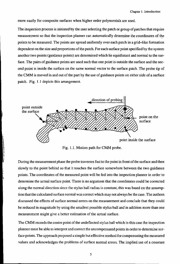
The inspection process is initiated by the user selecting the patch or group of patches that require
measurement so that the inspection planner can automatically determine the coordinates of the
points to be measured. The points are spread uniformly over each patch in a grid-like formation
dependent on the size and proportions of the patch. For each surface point specified by the system
another two points (guidance points) are determined which lie equidistant and normal to the sur
face. The pairs of guidance points are used such that one point is outside the surface and the sec
ond point is inside the surface on the same normal vector to the surface patch. The probe tip of
the CMM is moved in and out of the part by the use of guidance points on either side of a surface
patch. Fig. 1.1 depicts this arrangement.
direction of probing .. point on the surface
point inside the surface
Fig. 1.1. Motion path for CMM probe.
During the measurement phase the probe traverses fast to the point in front of the surface and then
slowly to the point behind so that it touches the surface somewhere between the two guidance
points. The coordinates of the measured point will be fed into the inspection planner in order to
determine the actual surface point. There is no argument that the coordinates could be corrected
along the normal direction since the stylus ball radius is constant, this was based on the assump
tion that the calculated surface normal was correct which may not always be the case. The authors
discussed the effects of surface normal errors on the measurement and conclude that they could
be reduced in magnitude by using the smallest possible stylus ball and in addition more than one
measurement might give a better estimation of the actual surface.
The CMM records the centre point of the undeflected stylus ball which in this case the inspection
planner must be able to interpret and correct the uncompensated points in order to determine sur
face points. The approach proposed a simple but effective method for compensating the measured
values and acknowledges the problems of surface normal errors. The implied use of a constant
5
Chapter 1. Introduction
value for probe deflection may not be valid as the magnitude of deflection varies according to
the attack angle [20,21]. However, the inspection planner does not detennine probe set-up, com
ponent set -up or collision-free safe rapid paths.
Van Den Berg [3] described the development of an automated machining cell to make small
batches of precision turbine parts. The automated machining cell was integrated with a CMM to
produce a flexible manufacturing system. To maximize productivity of the cell the time to
measure and analyse a manufactured part needed to be less than the time required to manufacture
the next part. In order to achieve such an automated cell further areas such as automatic material
transfer, automatic inspection and automatic error analysis (this may include estimation of the
cause of error and determination of a correction strategy) needed to be considered.
Inspection of the part was carried out using both the machining centre's touch trigger probe and
the CMM to capture measurement data. A menu driven system allowed the user to interactively
develop inspection programs, however as with the previous system of Duffie et al. only points
could be measured. It is not clear whether there was any intelligent assistance in the detennination
of probing points, but the machining centre used a drilling cycle to measure, so each inspection
point needed to be formulated as part of a drill cycle. The measured points are sent to the cell
controller for interpretation by a user written programme which accesses the machine library of
analysis functions. Measurement data from both the machining centre and CMM are analysed
for error analysis.
The manufacturing analysis is a two step process. Firstly the observed errors should be matched
against the possible sources of error in the manufacturing process model, which creates a model
of how the errors observed in the measurements were caused. The second set-up invol ves the ap
plication of corrective strategies to the manufacturing process.
Two methods of error analysis are employed within the system; the first is tolerance analysis,
which determines whether the measured point is out of tolerance and the second is manufacturing
analysis, which detennines the cause of the error and a correction strategy. The tolerance analysis
facility is capable of checking for position, orientation and form errors by calculating the error
vector of each point with respect to the surface and then by detennining the transformation matrix
necessary to fit the measured points to the defined surface. The position and orientation errors
could be extracted from the net rigid body fitting transformation, from which the form errors
could be extracted from the error vectors.
6
Chapter I. Introduction
1.5 Vision directed inspection and recognition
In order to achieve a highly effective inspection system, the inspection process should be inter
faced to a machine vision. Machine vision endows an inspection system with a sophisticated sens
ing mechanism to respond to its environment in an intelligent and flexible manner. Vision inspec
tion can be defined as the process of extracting, characterizing, and interpreting information from
images of a 3-D world.
The application of computer-based image analysis is an emerging technology. Many useful ap
plications are possible with existing technology which include finding flaws, identifying parts,
detecting surfaces, guaging, determining X, Y, and Z coordinates to locate parts in three dimen
sional space for robot guidance and many other application [22]. Use of machine vision in a
manufacturing process not only can avoid the production of scrap but also improve quality of
production, reduce set-up time, increase equipment utilization and bring many other benefits.
The vision directed inspection has been studied by a number of researchers [6,8,23,24,25,26,27,
28,29]. Generally the major issue in this research area is the development of representation or
feature extraction of3-0 objects by fusing multi images of an object which are taken from differ
ent view points or from the same view point with different illumination.
The technique described by McMichael [23] represents an image intensity gradient in two de
rived maps of gradient magnitude and orientation. The initial research objective was to consider
techniques that are insensitive to poor lighting since the lighting is a neglected area in industrial
image processing and poor lighting is often taken to imply specular reflection, shadow, and low
image contrast. In the proposed method several images of the object to be inspected taken from
the same view point, but illuminated differently, are fused together to attenuate the effects of sha
dow and image contrast variation. The method appears to be faster and uses more of the informa
tion available from the gradient orientation map. The technique thresholds on gradient magnitude
and deletes regions of high variation of gradient orientation, which allows the edge segments to
be detected and can be shown graphically.
There is also too much information regarding edge regions (i.e., pixellocations). A method of
information compression is required to identify parametric edge segments by their orientation,
length and centre. The method of edge segment extraction using gradient magnitude and orienta
tion mapping can be achieved by either finding the segment orientation directly from the orienta
tion map or by determining the edge from the distribution of pixellocations. The former is per
ceived by the author to be useful for short edge regions and diffuse edges, while the latter gives
. highly accurate results with long straight edge regions. However, fusing the results of both
7
Chapter J. Introduction
methods improves reliability. Extracting an accurate gradient field from an image is not easy.
Such issues as orientation accuracy and bandwidth, a1iassing, edge intensity bandwidth, signal
to noise ratio and localisation need to be taken into account. The weaknesses of the system are
a reliance on global thresholds, computation time, and, lack of the powerful software to detect
complex edges. However, the system appears to be good at finding the edge structure of scenes
with straight edges and sharp corners, furthermore it seeks to extract information about objects
rather than images.
McDonald et al. [28] and Urquhart et al. [26] researched on methods concerned with stereo scene
coding or active animated stereo vision. In their work a set of hardware and software tools are
developed around the Active Stereo Probe (ASP) which uses structured pattern projection. Scene
objects are illuminated by patterns projected by the ASP Active Illumination Projection System
(AlPS). Images of patterns, disrupted by the scene, are then captured using the ASP stereo camera
head and analysed using a technique called Stereo Scene Coding (SSC) to recover 3-D informa
tion.
The ASP head consists of two cameras independently actuated. The AlPS which allows projec
tion of patterns onto the viewed scene, is positioned below the sensor head such that it projects
onto an inclined mirror situated between the cameras. The mirror is also actuated in elevation and
azimuth allowing the reflected structured illumination pattern to be steered so that it is maintained
within the camera's fields of view. The performance of the combined AlPS/ASP system is criti
cally dependent on the system's ability to project and image patterns. The overall model can pre
dict captured image characteristics relative to the projected pattern, given object reflection char
acteristics and details of ambient light conditions.
In SSC images the scene to be analysed is captured by the left and right cameras during the projec
tion of each pattern. Analysis of the distortions of each pattern are used to make 3-D measure
ments about scene points.
The complexity grade of the system is high and is believed to work once the system is set -up and
the cameras are calibrated. The quality of measurements made using stereo scene coding is direct-
1y dependent on the quality ofthe input pattern images. The field of the camera's view is a control
ling factor, however, the given accuracy of the order of ±0.5 mm RMS in height for 3 m range
is good. Although, the camera's focal lengths are 500 mm or more, it is not stated what would
be the top limit of the object size before the accuracy will deteriorate. The quality of measure
ments using SSC and performance of algorithm utilising the combined AISP/ ASP system is di
rectly dependent on the quality of image patterns, for example high quality input images (full
8
Chapter 1. Introduction
frequency content, high contrast ratio and high signal to noise ratios) result in high measurement
accuracy. Both the projection and imaging process are subject to corruption by noise and degrada
tion through loss contrast ratios and optical blurring.
Clarke et al. [25] discussed another 3-D measurement system using multiple camera views that
are obtained from different viewpoints. The work describes the basic method of photograrnmetry
[30,31,32] and discusses the potential for automated high accuracy measurement in an industrial
context. The method involves identifying homologous targets or patterns (i.e., reflective marks)
on images of an object which have been obtained from different viewpoints. These image mea
surements are then used to capture, the 3-D coordinates of the locations of the targets or patterns
on the object being measured. Each point on the object is related to a set of measurements made
in the image space by a set of colinear equations through the theory of a central perceptive projec
tion. Each colinearity equation contains unknowns such as: the location and orientation of the
camera at exposure time; the X, Y,Z coordinates of the object point; and its corresponding image
coordinates in 2-D X,Y image space.
Since real imaging systems only approximate to the central perspective projection, equations
must also be included to model departures such as those caused by the real lens system, and any
geometric distortion of the image due to the camera sensor characteristics.
There are a number of steps before measurement can take place such as; placement of target
points, setting cameras and lighting, collection of images from each view-point and estimation
of camera locations and orientations (position of the camera relative to the object). Further steps
are identification and labelling of the targets, calculation of correspondences between targets
from all viewpoints, initialisation of focal length, principal point position, lens distortion parame
ters, least squares adjustment with initial estimated parameters to check that the program con
verges and that the change in the coordinates is within some pre-determined limits. If this occurs
then the programme is terminated otherwise it is required to check for errors (i.e., incorrectly lo
cated targets or matched targets) and repeat the adjustment process with new adjusted values. The
resulting 3-D coordinates of the target points after determination are transferred into a CAD sys
tem and used to derive a 3-D B-spline surface.
The accuracy of the method is dependent on several factors including; the number of observa
tions, the type of target or surface feature, camera stability, the strength of the measurement net
work and operator experience. The system appears to be flexible, there is no limit to the size of
the measured object, and the measuring system is portable. The system has some disadvantages
such as the high level of computation involved, the significant setting up procedure required for
9
Chapter 1. Introduction
each measurement case, a high degree of expert knowledge, and the lack of techniques for fast
or dynamic automated measurement.
The 3-D object recognition from mUltiple views can be employed to build structured models of
bodies in a scene by identifying classes of simple objects (e.g., wedges, bricks, etc.) and their
interrelationships (e.g., in front of, next to, supported by, etc.) in each view to build a prototype
model. Martin and Aggarwal [33] used multiple views to build a volumetric model of 3-D ob
jects, although their algorithm allowed learning and refinement it required explicit knowledge
about each viewpoint during learning and recognition.
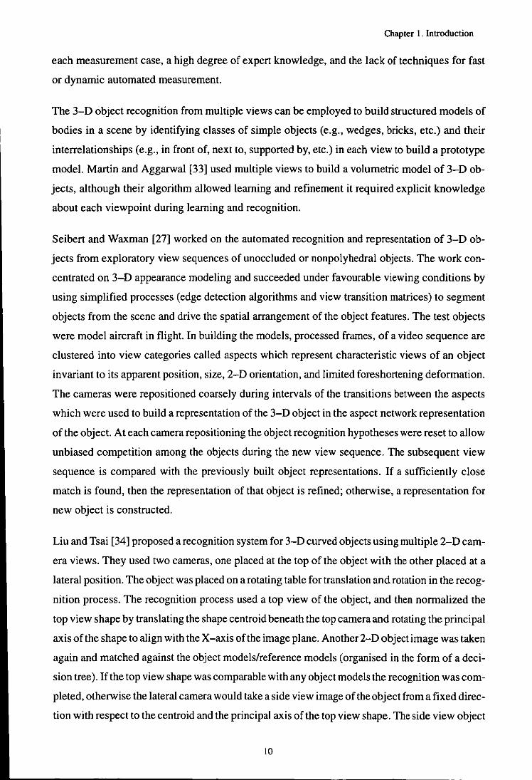
Seibert and Waxman [27] worked on the automated recognition and representation of 3-D ob
jects from exploratory view sequences of unoccluded or nonpolyhedral objects. The work con
centrated on 3-D appearance mode ling and succeeded under favourable viewing conditions by
using simplified processes (edge detection algorithms and view transition matrices) to segment
objects from the scene and drive the spatial arrangement of the object features. The test objects
were model aircraft in flight. In building the models, processed frames, of a video sequence are
clustered into view categories called aspects which represent characteristic views of an object
invariant to its apparent position, size, 2-D orientation, and limited foreshortening deformation.
The carneras were repositioned coarsely during intervals of the transitions between the aspects
which were used to build a representation of the 3-D object in the aspect network representation
of the object. At each camera repositioning the object recognition hypotheses were reset to allow
unbiased competition among the objects during the new view sequence. The subsequent view
sequence is compared with the previously built object representations. If a sufficiently close
match is found, then the representation of that object is refined; otherwise, a representation for
new object is constructed.
Liu and Tsai [34] proposed a recognition system for 3-D curved objects using multiple 2-D cam
era views. They used two cameras, one placed at the top of the object with the other placed at a
lateral position. The object was placed on a rotating table for translation and rotation in the recog
nition process. The recognition process used a top view of the object, and then normalized the
top view shape by translating the shape centroid beneath the top camera and rotating the principal
axis of the shape to align with the X-axis of the image plane. Another 2-D object image was taken
again and matched against the object models/reference models (organised in the form of a deci
sion tree). If the top view shape was comparable with any object models the recognition was com
pleted, otherwise the lateral camera would take a side view image of the object from a fixed direc
tion with respect to the centroid and the principal axis of the top view shape. The side view object
to

Chapter 1. Introduction
shape was then matched against side view shape of the object models for further discriminations.
This method uses features extracted from 2-D object shapes directly as the object model, this
accomplishes 3-D object recognition by matching sequentially input 2-D silhouette shape fea
tures against those of model shapes which have been taken from the set of fixed camera views.
The reason for this recognition of 3-D objects by 2-D silhouette shape is based on simple shape
features, but the learning process for the decision tree set up is not yet automated and needs to
be specifically arranged. However, the computation is not seen to be complicated and a high rec
ognition rate for most industrial parts is envisaged. Difficulties in recognizing a part could occur
due to an improper threshold selection for feature comparison, resulting in the assignment of in
put objects to incorrect tree nodes. Another source of error was the camera sensitivity to light
changes in the environment, resulting in undesirable changes of shape boundaries and object fea
tures. It was suggested that the above problems could be improved by the use of autoregressive
models to represent object boundaries, making features less sensitive to boundary distortions and
the adoption of sophisticated pattern classification algorithms to discriminate the object shapes
more radically. The proposed method may be employed for sculptured surface recognition, how
ever, it is not easy to install a rotary table on the CMM and measurement errors can occur because
of the rotary table. Also, if the object has a rotationally symmetric base, it is not easy to recognize
the object.
Al-Kindi et al. [6] have worked on automatic 2-D component inspection with assistance of ma
chine vision for engineering components. Their extensive work is based on the use of edge detec
tion with new developed algorithms for application when contour tracing methods fail to detect
localized edges in a complex scene. They restated that the use of 2-D object inspection using
computer vision can be approached in 3 ways: (1) an interactive approach where the user selects
and shows the required feature to be examined, (2) a teaching approach which assumes that the
system has previous knowledge of features to be inspected, (3) a full automated approach where
the system has no prior information about the object or its position.
In edge detection operations there are three types of error which sometimes cause the operation
to fail. These are: (1) missing valid edge points, (2) failure to detect localized edge points and
(3) failure to separate noise. The Edge Detection Algorithms (EDA's) are classified in two
groups, namely, differential type operators and model fitting methods. A new algorithm for edge
finding was proposed by the authors which they believed to be beneficial for most applications
where contour tracing fails to detect localized edges in a complex scene. It is not always obvious
which of the EDA's will be the most effective in a particular application unless tests for suitability
11
Chapter I. Introduction
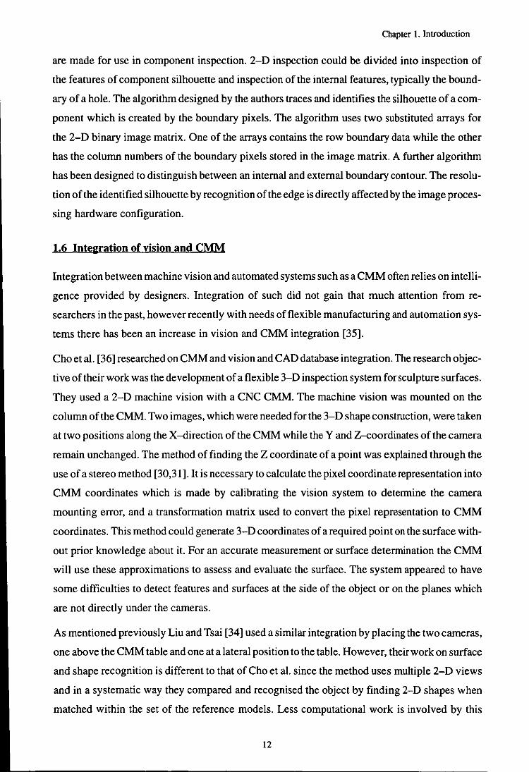
are made for use in component inspection. 2-D inspection could be divided into inspection of
the features of component silhouette and inspection of the internal features, typically the bound
ary of a hole. The algorithm designed by the authors traces and identifies the silhouette of a com
ponent which is created by the boundary pixels. The algorithm uses two substituted arrays for
the 2-D binary image matrix. One of the arrays contains the row boundary data while the other
has the column numbers of the boundary pixels stored in the image matrix. A further algorithm
has been designed to distinguish between an internal and external boundary contour. The resolu
tion of the identified silhouette by recognition of the edge is directly affected by the image proces
sing hardware configuration.
1.6 Intel:ration of vision and CMM
Integration between machine vision and automated systems such as a CMM often relies on intelli
gence provided by designers. Integration of such did not gain that much attention from re
searchers in the past, however recently with needs of flexible manufacturing and automation sys
tems there has been an increase in vision and CMM integration [35].
Cho et al. [36] researched on CMM and vision and CAD database integration. The research objec
tive of their work was the development of a flexible 3-D inspection system for sculpture surfaces.
They used a 2-D machine vision with a CNC CMM. The machine vision was mounted on the
column of the CMM. Two images, which were needed for the 3-D shape construction, were taken
at two positions along the X-<lirection of the CMM while the Y and Z-coordinates of the camera
remain unchanged. The method of finding the Z coordinate of a point was explained through the
use of a stereo method [30,31]. It is necessary to calculate the pixel coordinate representation into
CMM coordinates which is made by calibrating the vision system to determine the camera
mounting error, and a transformation matrix used to convert the pixel representation to CMM
coordinates. This method could generate 3-D coordinates of a required point on the surface with
out prior knowledge about it. For an accurate measurement or surface determination the CMM
will use these approximations to assess and evaluate the surface. The system appeared to have
some difficulties to detect features and surfaces at the side of the object or on the planes which
are not directly under the cameras.
As mentioned previously Liu and Tsai [34] used a similar integration by placing the two cameras,
one above the CMM table and one at a lateral position to the table. However, their work on surface
and shape recognition is different to that of Cho et al. since the method uses multiple 2-D views
and in a systematic way they compared and recognised the object by finding 2-D shapes when
matched within the set of the reference models. Less computational work is involved by this
12
Chapter I. Introduction
method, however more errors could be introduced since a rotary table is used.
1.7 CMM and CAD integration
CMM's are widely used tools for performing fast accurate measurements of industrial compo
nents. In order to achieve a high degree of flexibility and higher productivity in an automated
inspection environment an integration of a CNC CMM with a CAD system has a major role. The
primary objectives of such integration will be the development of techniques for automatically
generating inspection procedures from CAD data (off-line programming) and access to part de
sign (CAD) databases for quality assurance.
The concept of CMM and CAD integration has been around for less than a decade, its major ad
vantage is the reduction in inspection planning. Harris et al. [37] explained a type of integration
which allowed nominal and measured data to be exchanged between CAD and CMM systems
for graphical interactive programming of the CMM. The data exchange between these two sys
tems needed to be of a bidirectional data exchange standard such as DMIS [38].
Cowling and Mullineux [39] explained the type of information required for such integration.
They pointed out that the ability to transfer data between CAD and CMM systems requires intelli
gence of the human user by specifying the critical features and the inspection strategy for measur
ing them. In their study the CMM was simulated in software and the model of the component to
be inspected existed within the CAD system called "origin CAD model". The CMM held a second
model, the "physical component". Differences between these models represent errors in manu
facture.
By returning coordinates of the points between the physical model on the CMM and the probe
inspection path, a second model can be created within the CAD model. By interrogating the CAD
data from the third model geometric entities or features could be passed to the CAD system to
decide where faults were.
Their suggested solution strategies for CAD and CMM integration are concentrated on areas such
as data fitting, since the component may not comprise exact lines and arcs. Further work was con
cerned with determination of the end points of entities since they are in different positions to the
corresponding end points in the original CAD model and finally a recursive subdivision scheme
for inferring good representation of the entities of the physical component. Often the required
degree of accuracy could not be achieved if a small number of data points was used.
The issue of CAD and CMM interfacing was further investigated by Schwartz and Karadayi [40].
They designed and developed an intermediate system in the form of a translator buffer named
13

Chapter I. Introduction
Expert DIMS Graphical Editor Simulator (EDGES). They focused on problems that would be
expected once this integration took place, such as reduction in speed of inspection, robustness
of DMIS, and lack of operator knowledge. They considered operator difficulties in this area to
be considerable. The need for extensive system training of CMM personnel is significant since
the machine and system integration are complex.
1.8 Research objectives and proposed approach
There are many problems that must be addressed in the 3-D automated measurement of high
technology sculptured surfaces products such as, the type of sensing system to be used, the cost
effectiveness of the system, the degree of accuracy and the speed of measurement. If using a non
contact sensing method such as a vision system problems such as arranging a suitable lighting
system and developing image analysis methods for different applications have to be resolved. It
has been mentioned previously that vision systems are not flexible enough to be integrated cheap
ly and easily into an automated inspection environment for sculptured surfaces, because they do
not have the required capabilities for high accuracy. Therefore high accuracy applications are li
mited to the use of a touch probing approach. The automatic generation of NC code for this in
spection approach for the sculptured products presents an additional problem since it is a time
consuming business. One approach to overcome this problem is to use a cheap or inexpensive
2-D vision system which would give a first approximation to the location of the object features
and then use this information as an input to generate the NC drive code for a touch probe CMM.
The objective of this research is to develop an automated inspection system for the measurement
of sculptured surfaces using this approach. A number of secondary objectives were identified
which are;
1. Integration of the various elements.
2. A method for recognition and identification of the product features.
3. A method for NC dri ve code generation with a measurement optimisation procedure to achieve
accuracy and speed.
4. A suitable method of displaying the information graphically.
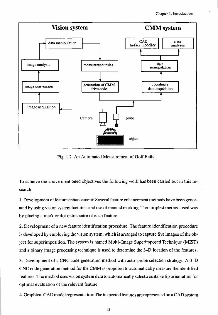
In order to develop the system a golf ball has been selected as the sample product since it contains
3 dimensional curved surfaces and features together with repeated surface patterns. The sche
matic diagram of the proposed inspection system is shown in fig. 1.2.
14
Vision system
data manipulation
image analysis
image conversion
image acquisition
measurement rules
generation of CMM drive code
Camera
Chapter I. Introduction
CMMsystem
CAD surface modeller
error analyses
object
data manipulation
coordinate data acquisition
Fig. 1.2. An Automated Measurement of Golf Balls.
To achieve the above mentioned objectives the following work has been carried out in this re
search:
1. Development of feature enhancement: Several feature enhancement methods have been gener
ated by using vision system facilities and use of manual marking. The simplest method used was
by placing a mark or dot onto centre of each feature.
2. Development of a new feature identification procedure: The feature identification procedure
is developed by employing the vision system. which is arranged to capture five images of the ob
ject for superimposition. The system is named Multi-Image Superimposed Technique (MIST)
and a binary image processing technique is used to determine the 3-D location of the features.
3. Development of a CNC code generation method with auto--probe selection strategy: A 3-D
CNC code generation method for the CMM is proposed to automatically measure the identified
features. The method uses vision system data to automatically select a suitable tip orientation for
optimal evaluation of the relevant feature.
4. Graphical CAD model representation: The inspected features are represented on a CAD system
15

Chapter I. Introduction
to visualise the results and for CAD and CMM data comparison.
5. Error model generation: Two applications of optimisation methods are proposed to model pat
tern errors. The model handles errors existing between the nominal and actual data. The fIrst
method uses a random search method technique to propose an optimum position for features pat
terns, the second method uses a least square best fIt strategy.
6. Experiments and results analysis: Several different types of golf balls and hobs were used and
their features identified and inspected automatically based on the proposed method of the vision
integrated CMM. Finally, the measured model is graphically represented and its error model gen
erated and analysed.
16
Chapter 2. Digital image processing system
CHAPTER 2
DIGITAL IMAGE PROCESSING SYSTEM
2.0 Introduction
Digital image processing is a term given to the process of analysing electronic images which are
taken by Charged Couple Device (CCD) sensors. The procedure is similar to normal photography
but instead of using a negative, the image is converted from an optical picture by use of a elec
tronic photo sensitive elements to a digital image. A digital image consists of a matrix of pixels
(a pixel is the smallest picture element i.e., photosite) which can be represented by 8 bits (a byte)
or higher order of gray level. The 8 bit gray level generates 256 shades of intensity which gives
an image of various shades, unlike people, who can interpret and characterise as many as 4000
colours/shades. Machine vision systems available today generally only interpret colours into the
shades of gray defined by the specific system [22]. They generally cannot distinguish between
object colours and can become confused if two colours have the same gray value.
The term computer vision (or machine vision) is a general name given to a system which includes
a digital image processing unit. The applications of computer vision are increasing at a fast rate,
and the use of these machines can be seen in industrial inspection, surface measurement, manipu
lator guidance, vehicle guidance, medical applications, civilian applications and the food in
dustry. One of the most difficult tasks facing image processing and computer vision is the devel
opment of systems that emulate the visual cognitive ability ·of high level biological visual
systems.
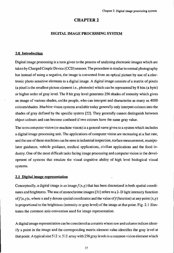
2.1 Digital image representation
Conceptually, a digital image is an imageJ(x,y) that has been discretized in both spatial coordi
nates and brightness. The use of monochrome images [31] refers to a 2-D light intensity function
ofJ(x,y)s, where x and y denote spatial coordinates and the value ofJ(function) at any point (x,y)
is proportional to the brightness (intensity or gray level) of the image at that point. Fig. 2.1 illus
trates the common axis convention used for image representation.
A digital image representation can be considered as a matrix where row and column indices ident
ify a point in the image and the corresponding matrix element value identifies the gray level at
that point. A typical size512 X 512 array with 256 gray levels is a common vision element which
17
Chapter 2. Digital image processing system
ongm ......
.f{x=O,y=O) .-------------.----'~
~ .f{x,y)
x
y
Fig. 2.1. Axis and coordinate convention for digital image representation.
can be seen in the majority of current machine vision applications.
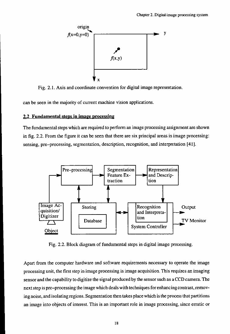
2.2 Fundamental steps in image processing
The fundamental steps which are required to perform an image processing assignment are shown
in fig. 2.2. From the figure it can be seen that there are six principal areas in image processing:
sensing, pre-processing, segmentation, description, recognition, and interpretation [41].
Pre-processing Segmentation Representation Feature Ex- and Descrip-traction tion
, Image Ac- Storing Recognition 0 quisition/ and Interpreta-Digitizer I Database I tion
L...::!. T System Controller
Object
utput
V Monitor
Fig. 2.2. Block diagram of fundamental steps in digital image processing.
Apart from the computer hardware and software requirements necessary to operate the image
processing unit, the first step in image processing is image acquisition. This requires an imaging
sensor and the capability to digitize the signal produced by the sensor such as a CCD camera. The
next step is pre-processing the image which deals with techniques for enhancing contrast, remov
ing noise, and isolating regions. Segmentation then takes place which is the process that partitions
an image into objects of interest. This is an important role in image processing, since erratic or
18

Chapter 2. Digital image processing system
weak segmentation algorithms almost always result in eventual failure. A robust or rugged seg
mentation procedure is an important factor in the successful solution of imaging problems. The
output of the segmentation stage is usually raw pixel data which needs converting into a suitable
form for computer processing. However, the image segmentation either comprises all the points
in the region or constitutes the boundary of a region.
After segmentation, representation and feature extraction takes place. This section deals with the
computation of features (e.g. size and shape) suitable for differentiating one type of object from
another. The data can represent a boundary when the focus is on external shape characteristics,
such as corners, straight edges, or concave to convex curvatures. It can also represent a complex
region which is more appropriate for representing internal properties, such as texture and struc
ture or skeletal shape.
The main task of representation is to transform the raw data into a suitable form for subsequent
processing. In order to achieve this a complementary method should also be specified for describ
ing the data so that the features of interest can be selected. Extracting features from a class of
objects in an image needs descriptors which are called feature selectors. These feature selectors
can also help to differentiate one part of the feature from another. The final processing stage in
volves recognition and interpretation, the former is the process that identifies and assigns a label
to an object based on the information provided by its descriptors while the latter assigns meaning
to a collection of recognized objects.
The knowledge is stored in a database which may interact with processing modules individually.
The system can operate with simple or complex knowledge which would be fedback to the rel
evant module in order to enable the module to process the task better. For example if the process
is in the segmentation or representation module the problem can be resolved for a better bounding
representation or a region representation. The feature knowledge can refer to regions of an image
where the interested information is known to be located, therefore the search can be easily con
ducted in seeking information, whereas in images with unknown and interrelated regions in
formation is not so easily detectable.
It is important to note that not all image processing applications require the complexity of interac
tions shown in fig. 2.2.
2.3 Vision system and its elements
In image sensing a sensor converts visual information into electrical signals (voltage signals). A
CCD sensor is composed of discrete silicon imaging elements, called photosites, that have a volt-
19

Chapter 2. Digital image processing system
age output proportional to the intensity of the incident light. The output voltages are amplified
and input to an AnaloglDigital Converter (NOC) in which the system characterizes the scene into
a grid of digital numbers. This process is called digitizing, or sometimes image samplinglquantiz
ing. The amplitude digitization is called intensity or gray level quantization. This is applicable
to monochrome images and reflects the fact that these images vary from black to white in shades
of gray. For a more detailed description of these processes references [22,31,41] provide ad
equate explanations.
The sections of a simple vision system can be listed as; acquisition, storage, processing, com
munication, and display. The image acquisition section is usually a CCD sensor coupled with AI
DC as mentioned earlier. The digital storage for image processing can be divided into three sec
tions; temporary (short term storage for use during processing), on-line storage (for relatively
fast recall), and archival storage for any time access. Storage is measured in bytes (8 bit), for an
eight bit image of size 512 X 512 pixels about 1/4 of a million bytes of storage are required. In
processing generally the image will go through various operations including, image enhance
ment, coding, and analysis. These processes can be handled in hardware or in software and the
processes are usually expressed in algorithmic form, the hardware implementation is often faster
than software execution but with less flexibility.
Communication in digital image processing performs local or network communication between
image processing systems and remote communication from one point to another. To be able to
implement such a connection hardware and software requirements of the standard communica
tion protocol needed to be considered. Finally, the display section shows the digital images, com
mon examples are monochrome and colour television monitors which are used in modem image
processing systems. The display unit is fed by the output from the image display module hardware
which is situated in the host computer of the image system. However, there are other sorts of dis
play such as slides, photographs, and transparencies:
2.4 Machine vision fundamentals
There are a number of aspects to be considered prior to processing of digital images, examples
of these are illumination, reflection effects, uniform image sampling, gray level quantization,
relationships between pixels (i.e., connectivity or distance measurement) and imaging geometry.
Illumination has a direct effect on the image processing and suitable images for processing are
those with a high contrast images, low specular reflections, low or no shadows and no extraneous
details. This could be a reason why arbitrary lighting of the environment is often not acceptable.
A good lighting system illuminates a scene so that the complexity of the resulting image is mini-
20
Chapter 2. Digital image processing system
mised, while the infonnation required for object detection and extraction is enhanced. The light
ing system is usually dictated by the application, specifically, the properties of the object itself
and the task, such as inspection, flaw checking, counting objects, character recognition or robot
control.
As mentioned earlier image sampling or digitization and quantization are required for computer
image processing. The most important point is that for consistent and unifonn output sampling
and quantization of an image. A suitable mathematical fonn should be used since a digital image
is a 2-D function whose spatial coordinates of the pixels and amplitude value of each pair is now
in the fonn of integers rather than analog. Apart from the above mentioned functions it is also
required to specify the number of discrete gray levels to display the image. This point is worth
considering before purchasing image processing software since the degree of discernible detail
(resolution) of an image depends on above mentioned parameters. This is one reason for the
number of image processing softwares which work on 256 gray levels and a resolution of
512x512 (square type).
There are some basic rules which need to be considered about pixels in a digital image such as
neighbours, and connectivity which can be used for detailed image processing. Specific arrange
ments can be made to use these pixel relationships to detect edges, feature measurements, and
labelling of connected components which would establish boundaries of objects and components
of regions in an image. Further processes are used for extra pixel manipulation such as arithmetic
and logic operations, the fonner works on multi-valued pixels (i.e., grey level) and the latter ap
plies only to binary images. These operations are used in most branches of image processing in
order to analyse shape, feature detection, filtering, and for masking purposes. Arithmetic opera
tions can be grouped as addition, subtraction, multiplication, and division of pixels and the princi
pal logic operations are AND, OR, and COMPLEMENT which are functionally complete and
they can be combined to fonn any other logic operation.
Another set of operations belong to image geometry which mainly involves transfonnations used
in imaging. These operations can be used to deal with problems involving image rotation, scaling,
translation, perspective transfonnations, camera position (which deals with two coordinate sys
tems, the camera and the world coordinate systems) and camera calibration [31].
21

Chapter 2. Digital image processing system
2.5 Review on vision systems for measurements of objects
Machine vision has developed extensively since its uncertain beginnings in the 1980s. At that
time systems were costly and early machine vision systems worked well in the laboratory but
were unable to cope with the vibration and dust of the production environment. After overcoming
the difficulties in transferring benchtop technologies to real world working environments ma
chine vision systems are now being applied increasingly to applications in the following in
dustries: automation, inspection, measurements, defence, electronic, food, health care, medical
(pathology and life sciences), pharmaceutical, security and, to many other fields of technology.
The biggest end users of industrial vision systems are the electronics sectors, with the automotive
industry in the second place. In electronics, production values are high and the implications of
product failure can be severe, thus a need for 100 per cent quality inspection is essential. A vision
system will not only identify faulty components but the system can also produce immediate stat
istical information on the type of rejects (e.g., measured dimensions). The investment in machine
vision can generally only be cost effective for high volume production. One main location when
using machine vision systems in the production lines is at the exit, w here products can be checked
for inadequate marking or wrong packing [42].
Currently the implementation of neural networks in vision system applications for developing
expert systems is taking place. They are predicted to be common in system controllers and pro
cessors by the year 2000. This is why the Department of Trade and Industry (DTI) is investing
3.75 million pounds over the next 3 years to promote industrial awareness in the use of neural
network [43]. Examples of these implementations are in signature verification, identification,
food processing, and vision inspection where grading of fruit using a vision system and neural
network uses surface defect classification techniques.
In measurement applications machine visions are applied at various degrees in detailed and com
plex measurement applications [44,45] where relatively high orders of accuracy are not required
(of the order of one millimetre). Typical application areas are measurement of chocolate bars;
grading of vegetables for size and even in automated butchery [46] where the locations and size
of each beef forequarter is determined prior to cutting. The inspection industry is focusing [47]
on how the vision information can be modelled and used in other industries. This arguably would
imply the use of a computer network based on an emerging communication standards. This will
resolve problems such as how the data can be transferred between vision machines and other com
puter systems.
Svetkoff et al. [48] and Mahon [8] employed vision system in the electronics industry to inspect
22
Chapter 2. Digital image processing system
component boards and solder pastes on surface mount printed circuit boards, where 100 per cent
inspection is required. Svetkoff et al. utilised a combination of gray scales and a 3-D sensing sys
tem to check minimum solder paste content and alignment of the paste to nominal pad locations.
The examples given indicate that when the contrast is low, inspection will generally require to
implement high speed 3-D information which could be based on a triangulation method. Mahon
considered the volume of paste, mean paste height, and individual pad measurement vectors. The
printed circuit boards were viewed under the camera and the board alignment was done by place
ment of the fiducial marks on the board at different locations. The detection of these marks was
made by the vision system and the recognition procedure took place by comparing the component
marks in a CAD database system. From the results the type of board and the locations for the
inspection of the pastes could be determined. 2-D and 3-D algorithms were used to calculate the
locations of pads in X and Y directions, the area and centriods of each pad were individually
measured. From knowing the location of each pad a grey level threshold for the area could be
set using the grey scale histograms of the paste and background images which could lead to an
area measurement. To calculate the height of the blob a structured light technique similar to Svet
koff et al. was used. The inspection system seems fast and effective although the averaging
method which was designed to give a higher degree of accuracy was questionable since blobs are
not square in practice and they might not be spread consistently in their positions as assumed in
the article. The system also experienced some difficulties to process light colour boards.
Blake [49] used a vision system in conjunction with two separate intersecting arrays oflight from
different projectors. This arrangement was used to digitise awkward 3-D shapes. Each of the pro
jectors transmits a set of fringes at right angles to each other. The camera picks up the images of
the two projections separately, and the grid intersection points are then be determined by the use
of projective geometry.
At Georgia Institute of Technology various researchers have employed machine vision to do in
telligent tasks. Brown [50] used a vision system to help mobile robots home in on targets without
following predetermined guide paths, by using prior knowledge of the environment. This robot
guidance system used a video camera with a series of algorithms for image processing. The over
all process followed a sequence which would find a potential workstation location, compare its
image with a stored model, guide the robot to approach the target, and then slow it down for dock
ing.
Pastorius [51] used a machine vision for surface quality inspection of objects up to 8 (feet) in
length. The system could analyse magnified surface waves of the order of magnitude of 50 mi-
23

Chapter 2. Digital image processing system
crons. The computer system provided a number of analysis algorithms for quantifying the gray
scale waviness seen in the images. Two panel masters were selected for calibration and assigned
values of "0" and "100", then test plaques (i.e., plastic, metal, or composite materials) were tested
and rated in relation to these masters.
As the use of machine vision in industries is increasing improvement of these non-contact sys
tems have been faster than the demand. Work has been done on making a smart vision camera
[52] which consists of a computer that does some image analysis before the data leaves the cam
era. However, what the manufactures have been really waiting for, is higher resolution solid-state
CCD cameras with resolution above 1000 X 1000 and their price is currently too high for many
users.
2.6 The vision system used for this work
A measuring system has been developed which is primarily based on a CMM, a touch trigger
probe, and a vision system. The vision system used for this work consists of a 2-D CCD sensor
Matrox MVP-AT, and an illumination system equipped with a filtering system.
2.6.1 The Matrox vision system
The Matrox vision system includes a vision board, a CCD camera with a 25 mm lens and a Hitachi
mono visual display unit. The vision system board operates in an mM-PC environment run by
the Matrox software. The board requires two adjacent 16 bit AT slots for installation and occupies
64 Kbytes of memory location and thirty two 8 bits 110 locations in the host computer address
space. The system software consists of:
1. Control packages to control the CMM (will be discussed in Chapter 3).
2. Imager-AT vision system.
3. PC-IMAGE vision software for vision analysis.
4. A developed programme named MARZ for vision analysis.
5. A developed programme named BALLINSP for golf ball inspection.
The software Imager-AT [53] is a software library which contains a set of primitive imaging
buffer arrangement, graphics and 110 commands for image processing. The software has libraries
of routines which can be used off line together with any other necessary programmes written in
the "C" language.
The original image buffer provided by the software consists of a 1024 X 1024 image frame buffer
with each pixel being 8 bits to represent intensity levels. The system program divides this frame
24
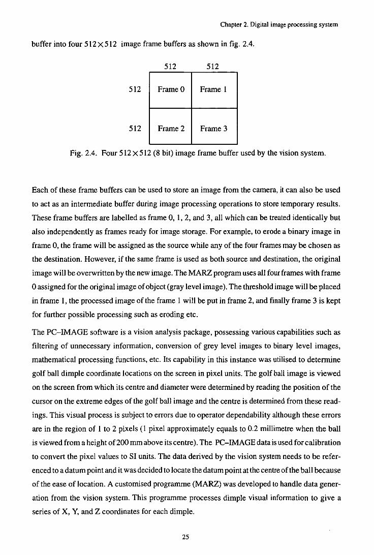
Chapter 2. Digital image processing system
buffer into four 512 X 512 image frame buffers as shown in fig. 2.4.
512 512
512 Frame ° Frame 1
512 Frame 2 Frame 3
Fig. 2.4. Four 512 X 512 (8 bit) image frame buffer used by the vision system.
Each of these frame buffers can be used to store an image from the camera, it can also be used
to act as an intermediate buffer during image processing operations to store temporary results.
These frame buffers are labelled as frame 0, 1, 2, and 3, all which can be treated identically but
also independently as frames ready for image storage. For example, to erode a binary image in
frame 0, the frame will be assigned as the source while any of the four frames may be chosen as
the destination. However, if the same frame is used as both source and destination, the original
image will be overwritten by the new image. The MARZ program uses all four frames with frame
° assigned for the original image of object (gray level image). The threshold image will be placed
in frame 1, the processed image of the frame 1 will be put in frame 2, and finally frame 3 is kept
for further possible processing such as eroding etc.
The PC-IMAGE software is a vision analysis package, possessing various capabilities such as
filtering of unnecessary information, conversion of grey level images to binary level images,
mathematical processing functions, etc. Its capability in this instance was utilised to determine
golf ball dimple coordinate locations on the screen in pixel units. The golf ball image is viewed
on the screen from which its centre and diameter were determined by reading the position of the
cursor on the extreme edges of the golf ball image and the centre is determined from these read
ings. This visual process is subject to errors due to operator dependability although these errors
are in the region of I to 2 pixels (1 pixel approximately equals to 0.2 millimetre when the ball
is viewed from a height of 200 mm above its centre). The PC-IMAGE data is used for calibration
to convert the pixel values to SI units. The data derived by the vision system needs to be refer
enced to a datum point and it was decided to locate the datum point at the centre of the ball because
of the ease of location. A customised programme (MARZ) was developed to handle data gener
ation from the vision system. This programme processes dimple visual information to give a
series of X, Y, and Z coordinates for each dimple.
25
Chapter 2. Digital image processing system
The data containing the coordinate positions of dimples with reference to the golf ball centre is
output to a file for use on the CMM. In order to accurately measure the dimples on tbe CMM,
a customised program named BALLINSP was developed. This software is used in collaboration
with tbe CMM initialise software MM4IDCC-315, tbe two combined programs examine the
coordinate location of each dimple, select a suitable tip orientation and then complete the inspec
tion procedure.
2.6.2 Illumination and filtering system
Illumination of a scene is an important factor in image processing since a badly illuminated object
often requires complex vision processing algorithms and techniques to provide high contrast and
minimise reflections and shadows whereas a suitable illuminated object would require fewer pro
cessing algorithms to generate a similar result [54]. To use an illumination system for image pro
cessing several general principles need to be considered [I], the most important of them being;
the output light level from the lamps, the spectral responses of the various optical components
(e.g. lenses, filters, etc.), the reflectivity of the object being examined as a function of wavelength
(i.e., its colour) and its smoothness, the spectral response of the image sensor, the performance
of the camera, the spatial distribution of the light (i.e., uniformity), the polarisation of the light,
the magnification of the optical system and the resolution of the digital images which are to be
used. It should be noted that in image processing it is often cheaper to improve tbe lighting system
than the image processing.
For high accuracy measurement the effect of the type of illumination on edge definition must be
considered. The arrangement of the illumination system can cause the illumination to be partially
coherent which can cause the measured edge position not to be detected.
The basic types of lighting devices may be grouped into the followings:
i) Diffuse surface devices (typically fluorescent lamps and light tubes).
ii) Condenser projectors (transforms an expanding light source into a condensing light source).
iii) Flood or spot projectors (used to illuminate large surface areas).
v) Collimators (used to provide a parallel beam of light on the subject).
vi) Imagers (such as slide projectors and optical enlargers).
The lighting system which was required for this instance should have the capability to generate
uniform contrast for the features on the golf ball surface and should illuminate the object in order
to provide uniform, shadow free, and ornni directional illumination. The difficulties experienced
26
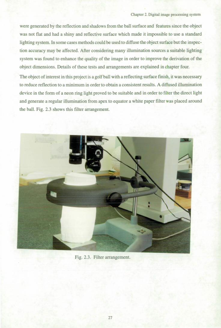
Chapter 2. Digital image processing system
were generated by the reflection and shadows from the ball surface and featu res since the object
was not flat and had a shiny and reflective surface which made it impossible to use a standard
lighting system. In some cases methods could be used to diffuse the object surface but the inspec
tion accuracy may be affected. After considering many illumination sources a suitable lighting
system was found to enhance the quality of the image in order to improve the derivation of the
object dimensions. Details of these tests and arrangements are explained in cbapter four.
The object of interest in this project is a golf ball witb a reflecting surface fmish, it was necessary
to reduce reflection to a minimum in order to obtain a consistent results. A diffused illumination
device in the form of a neon ring light proved to be suitable and in order to fil ter tbe direct ligbt
and generate a regular illumination from apex to equator a white paper filter was placed around
the ball. Fig. 2.3 shows this filter arrangement.
Fig. 2.3. Filter arrangement.
27
Chapter 3. Coordinate Measuring Machine
CHAPTER 3
COORDINATE MEASURING MACHINE (CMM)
3.0 Introduction
CMMs are multi-axis devices with two to six axes of movement, each of which provides an out
put of position or displacement. These machines are available in both manual and automatic
(computer controlled) models and are available in a wide range of sizes to provide for a variety
of applications. They were designed to record the position of a probe as it moved along its coordi
nate axes, and also to probe points in 3-D space and give the position of the touched point or the
centre of the probe point to micron accuracy. Softwares associated with CMMs enable them to
alter the situation for different measurements rather than altering equipment mechanics or elec
tronics. CMMs also have some means of providing output to the user (printer and etc.) and to
other machines in a complete manufacturing system. The main objectives of CMMs are to
measure and inspect complex 3-D components for both prismatic and sculptured surfaces.
A CMM can rapidly and accurately measure objects of widely varying size and geometric con
figuration, and can also measure the many different features of a part, such as holes, slots, studs
without needing a range of tools. More importantly if any changes need to be made in a fixed
measurement system for any reason this would increases the inspection cost and the time, how
ever changes in the measurement or inspection routine of a CMM can be made simply by editing
the computer programme that controls the machine. This flexibility and versatility is one of the
principal advantages of CMMs. They have been manufactured with different structures and con
figurations which all work under the same principle. They are similar in concept to CNC machine
tools which require a rigid construction with accurate positioning and sensors, direct current
(DC) drives and an intelligent controller capable of performing data processing and communica
tion tasks.
Although CMMs have shown they are good tools for performing fast accurate three dimensional
measurements of mechanical components they may not always be suitable if the user cannot pro
vide the correct operating environment, which is one of many primarily factors which affect
CMM performance.
To use the full potential of these machines linking them to CAD systems will enable more effi
ciency, flexibility and benefits, for example; inspection programs can be developed on the CAD
28

Chapter 3. Coordinate Measuring Machine
system and transferred to the CMM. Actual inspection data can be transferred from a CMM to
a CAD system which could enable comparison of nominal data with actual part information [55].
The major aim of bringing CMMs to the point of production was to control the production process
more fully. They play a vital role in the mechanisation of the inspection process and their tradi
tional role as a 3-D measurement tool is expanding since they offer potentially viable solutions
to a number of disputes facing manufacturers [36] such as;
i) The need to integrate quality management more closely into the manufacturing process.
ii) The realisation that the measurement process itself needs to be monitored and verified.
iii) The elimination of fixtures and fixed gauges thus providing increased gauging flexibility:
3.1 CMM and it's elements
The CMM must be rigidly built to minImise errors introduced by unintended movements between
the machine members and their movement along the axes of travel. Prior to considering the CMM
elements it is important to stress that this type of inspection machine requires special foundations
which may be several metres deep since they are generally delicated pieces of equipment and their
installation and usage need careful attention. The main components in a CMM are the base or bed,
column, bearings, scales and encoders, probes, control consols/monitoring units, hardware and
the software.
The base or bed is used for mounting or locating components, is generally made of granite for
maximum stability and is usually provided with tapped holes for clamping purposes. The base
stands on anti vibration mounts to absorb possible vibrations from within or from outside. In the
past, it was essential that the bed of the measuring machine be perfectly flat, but with the advent
of computer based error compensation, this characteristic has become far less vital.
The column will differ according to the type of CMM and generally comes as a square frame or
gantry to support the complete machine head and attachments. It should have enough stability
to withstand sudden shocks which could be generated from moving the head and the probe.
Bearings have a direct impact on the accuracy of all CMMs because of their effect on every mo
tion of the machine along its axes. The current bearing assemblies in measuring machine can be
the air or roller type, in a laboratory or a clean room where dust and dirt is minimum, air bearings
are the best choice, since they move without friction and are therefore the most accurate.
The scales and encoders of CMMs show where the probe is located within the work envelope of
the machine. There are mainly two types of scales, metal scales (stainless steel) and glass scales.
The most accurate scales are glass sinceit easily polished, stable, and able to work with both trans-
29

Chapter 3. Coordinate Measuring Machine
mitted and reflected light. The ordinary glasses have expansion coefficients 15 to 30 per cent less
than steel, and some special types have been developed which have the same expansion coeffi
cient as steel. This material permits finer etching of measurement lines than steel or other com
monly used materials.
Probes and sensors are the devices through which CMMs collect their measurement input. A wide
variety of probes are currently available. Each of these probes has its own application and pecu
liarity. Apart from non contact probes such as laser probes and vision probes, there are contact
probes such as hard probes, Touch Trigger Probes (TIPs), and CNC continuous contact probes
[56].
The control system on CM Ms is computer based and the machine motion can be operated from
the computer keyboard or more usually from control consols. The control consols on CMMs are
usually a hand held box Goy-sticks) with several function buttons. Some of the important func
tions of this unit are to allow the operator to take the probe to a start or a rest position, datum the
probe and perform other manual tasks such as aligning the workpiece.
The computer technology has been given capabilities and versatility that are rapidly making
CMMs essential to efficient manufacturing. Together the computer and the software programme
manipulates the data gathered by the CMM into the forms required by the user. In addition, the
computer also operates the CMM in DCC applications and functions automatically compensating
for errors within the structure of the machine.
3.2 Types of probes and sensors used by CMMs
CMMs have evolved in one decade, from simple layout machines with manually operated sys
tems, to highly accurate, automated inspection systems. A major factor in this evolution has been
the development of 3-D probes and sensors for both contact and non contact applications together
with motorised probe heads and automatic probe exchange system for unmanned, flexible inspec
tion.
The probing system on a CMM consists of the probe, the stylus and the application software
employed in using the probe [52,57,58]. In order to optimise the measuring performance of any
probe system, it is important that potential sources of error associated with the techniques used
are identified and the effects of probe application variants (stylus choice, trigger forces etc.) are
quantified. The ANSII ASME B891.1.12M [59] quotes" A major factor contributing to the total
system measuring error (of a CMM) is the performance of the total probing system ... ". Obviously
there are different types of probes with different technology, generally they are classified in two
30
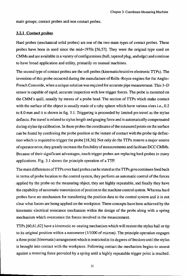
Chapter 3. Coordinate Measuring Machine
main groups; contact probes and non contact probes.
3.2.1 Contact probes
Hard probes (mechanical solid probes) are one of the two main types of contact probes. These
probes have been in used since the mid-1970s [56,57]. They were the original type used on
CMMs and are available in a variety of configurations (ball, tapered plug, and edge) and continue
to have broad application and utility, primarily on manual machines.
The second type of contact probes are the soft probes (kinematic/resistive electronic TIPs). The
invention of this probe occurred during the manufacture of Rolls-Royce engines for the Anglo
French Concorde, when a unique solution was required for accurate pipe measurement. This 3-D
sensor is capable of rapid, accurate inspection with low trigger forces. The probe is mounted on
the CMM's quill, usually by means of a probe head. The section of TIPs which make contact
with the surface of the object is usually made of a ruby sphere which have various sizes i.e., 0.2
to 8.0 mm and it is shown in fig. 3.1. Triggering is proceeded by limited pre travel as the stylus
deflects. Pre travel is related to stylus length and gauging force and is automatically compensated
during stylus tip calibration. In these probes the coordinates of the measured points on the surface
can be found by combining the probe position at the instant of contact with the probe tip deflec
tion which is required to trigger the probe [18,36]. Not only do the TIPs remove a major source
of operator error, they greatly increase the flexibility of measurements and facilitate DCC CMMs.
Because of their significant advantages, touch trigger probes are replacing hard probes in many
applications. Fig. 3.1 shows the principle operation of a TIP.
The main differences of TIPs over hard probes can be stated as the TIPs give continues feed back
in terms of probe location to the control system, they perform an automatic control of the forces
. applied by the probe on the measuring object, they are highly repeatable, and finally they have
the capability of automatic transmission of position to the machine control system. Whereas hard
probes have no mechanism for transferring the position data to the control system and it is not
clear what forces are being applied on the workpiece. These concepts have been achieved by the
kinematic electrical resistance mechanism within the design of the probe along with a spring
mechanism which overcomes the forces involved in the measurement.
TIPs [60,61,62] have a kinematic re-seating mechanism which will restore the stylus bailor tip
to its original position within a nanometer (1/1000 of micron). The principle operation engages
a three point (kinematic) arrangement which is restricted in its degrees of freedom until the stylus
is brought into contact with the workpiece. Following contact the mechanism begins to unseat
against a restoring force provided by a spring until a highly repeatable trigger point is reached.
31
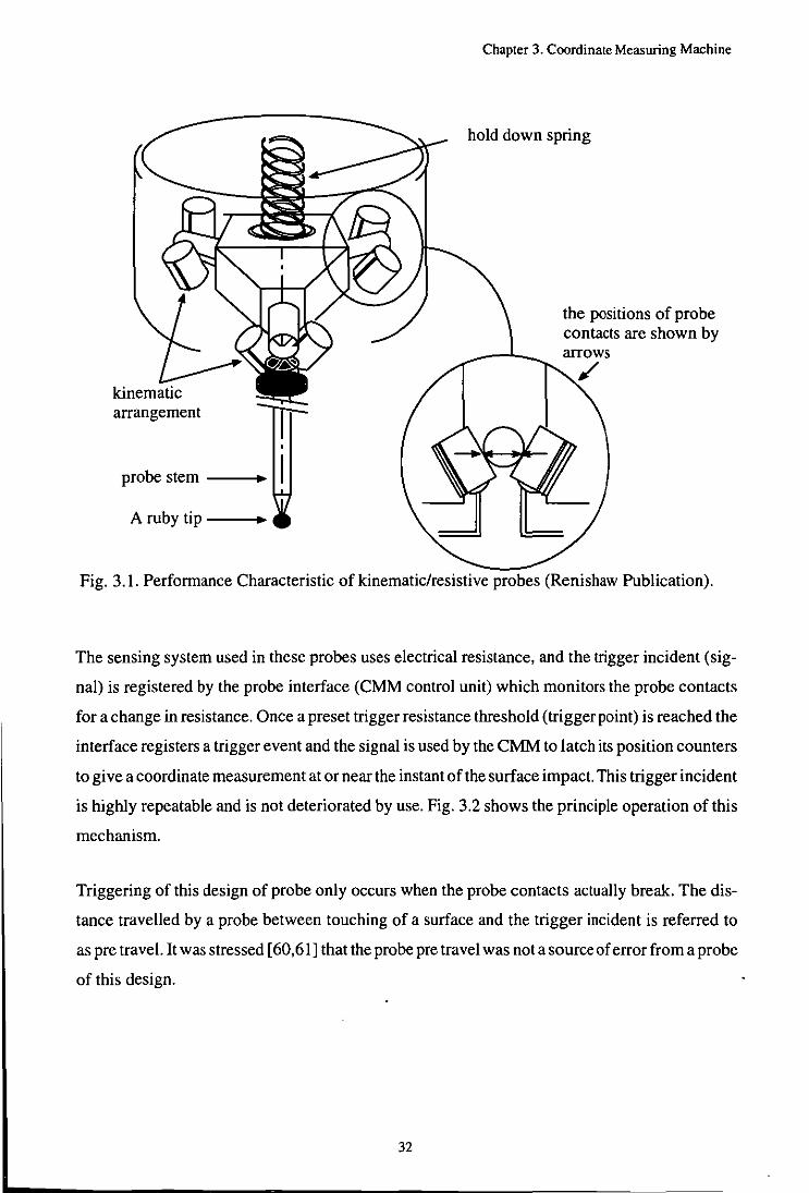
arrangement
probe stem --_
A ruby tip --.
Chapter 3. Coordinate Measuring Machine
hold down spring
the positions of probe contacts are shown by
Fig. 3.1. Performance Characteristic of kinematic/resistive probes (Renishaw Publication).
The sensing system used in these probes uses electrical resistance, and the trigger incident (sig
nal) is registered by the probe interface (CMM control unit) which monitors the probe contacts
for a change in resistance. Once a preset trigger resistance threshold (trigger point) is reached the
interface registers a trigger event and the signal is used by the CMM to latch its position counters
to give a coordinate measurement at or near the instant of the surface impact. This trigger incident
is highly repeatable and is not deteriorated by use. Fig. 3.2 shows the principle operation ofthis
mechanism.
Triggering of this design of probe only occurs when the probe contacts actually break. The dis
tance travelled by a probe between touching of a surface and the trigger incident is referred to
as pre travel. It was stressed [60,61] that the probe pre travel was nota source of error from a probe
of this design.
32
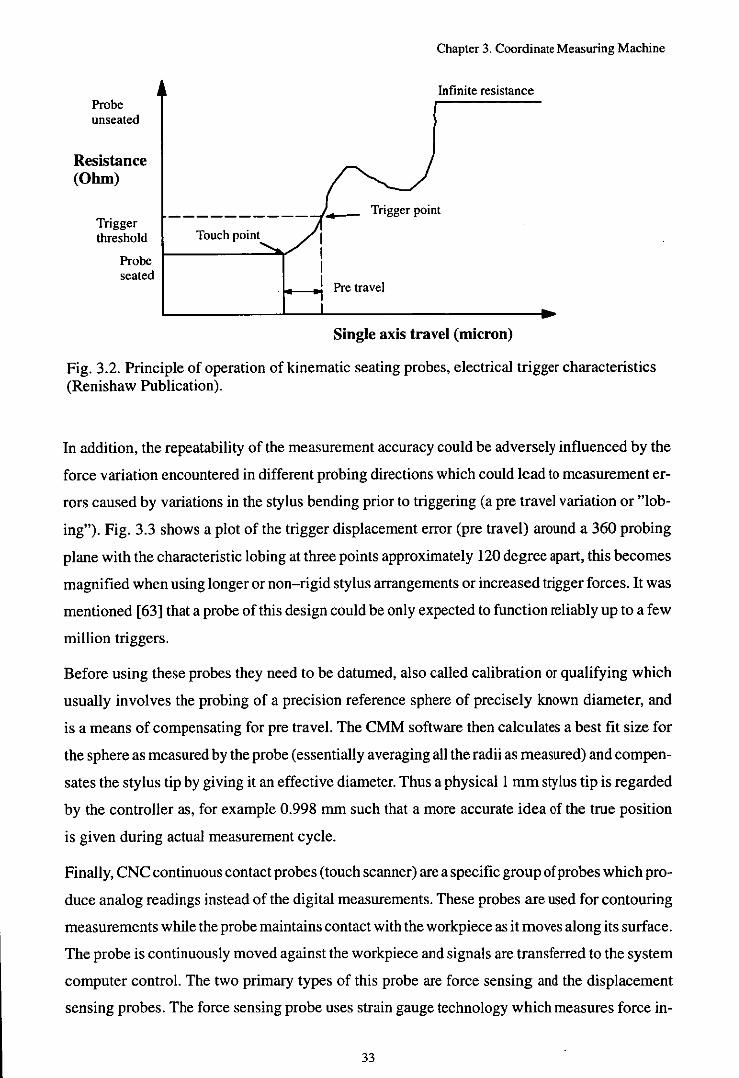
Probe unseated
Resistance (Ohm)
Trigger threshold
Probe seated
Touch point
Chapter 3. Coordinate Measuring Machine
Infinite resistance
Trigger point
Pre travel
Single axis travel (micron)
Fig. 3.2. Principle of operation of kinematic seating probes, electrical trigger characteristics (Renishaw Publication).
In addition, the repeatability of the measurement accuracy could be adversely influenced by the
force variation encountered in different probing directions which could lead to measurement er
rors caused by variations in the stylus bending prior to triggering (a pre travel variation or "Iob
ing"). Fig. 3.3 shows a plot of the trigger displacement error (pre travel) around a 360 probing
plane with the characteristic lobing at three points approximately 120 degree apart, this becomes
magnified when using longer or non-rigid stylus arrangements or increased trigger forces. It was
mentioned [63] that a probe of this design could be only expected to function reliably up to a few
million triggers.
Before using these probes they need to be datumed, also called calibration or qualifying which
usually involves the probing of a precision reference sphere of precisely known diameter, and
is a means of compensating for pre travel. The CMM software then calculates a best fit size for
the sphere as measured by the probe (essentially averaging all the radii as measured) and compen
sates the stylus tip by giving it an effective diameter. Thus a physical! mm stylus tip is regarded
by the controller as, for example 0.998 mm such that a more accurate idea of the true position
is given during actual measurement cycle.
Finally, CNC continuous contact probes (touch scanner) are a specific group of probes which pro
duce analog readings instead of the digital measurements. These probes are used for contouring
measurements while the probe maintains contact with the workpiece as it moves along its surface.
The probe is continuously moved against the workpiece and signals are transferred to the system
computer control. The two primary types of this probe are force sensing and the displacement
sensing probes. The force sensing probe uses strain gauge technology which measures force in-
33
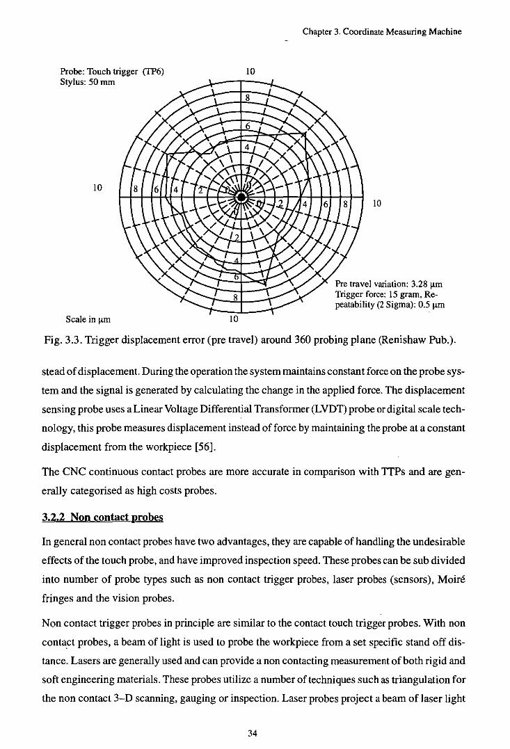
Probe: Touch trigger (TP6) Stylus: 50 mm
10
Scale in !lill 10
10
Chapter 3. Coordinate Measuring Machine
10
Pre travel variation: 3.28 !lill Trigger force: 15 gram, Repeatability (2 Sigma): 0.5 !lill
Fig. 3.3. Trigger displacement error (pre travel) around 360 probing plane (Renishaw Pub.).
stead of displacement. During the operation the system maintains constant force on the probe sys
tem and the signal is generated by calculating the change in the applied force. The displacement
sensing probe uses a Linear Voltage Differential Transformer (LVDT) probe or digital scale tech
nology, this probe measures displacement instead of force by maintaining the probe at a constant
displacement from the workpiece [56].
The CNC continuous contact probes are more accurate in comparison with TTPs and are gen
erally categorised as high costs probes.
3.2.2 Non contact probes
In general non contact probes have two advantages, they are capable of handling the undesirable
effects of the touch probe, and have improved inspection speed. These probes can be sub divided
into number of probe types such as non contact trigger probes, laser probes (sensors), Moire
fringes and the vision probes.
Non contact trigger probes in principle are similar to the contact touch trigger probes. With non
contact probes, a beam of light is used to probe the workpiece from a set specific stand off dis
tance. Lasers are generally used and can provide a non contacting measurement of both rigid and
soft engineering materials. These probes utilize a number of techniques such as triangulation for
the non contact 3-D scanning, gauging or inspection. Laser probes project a beam of laser light
34
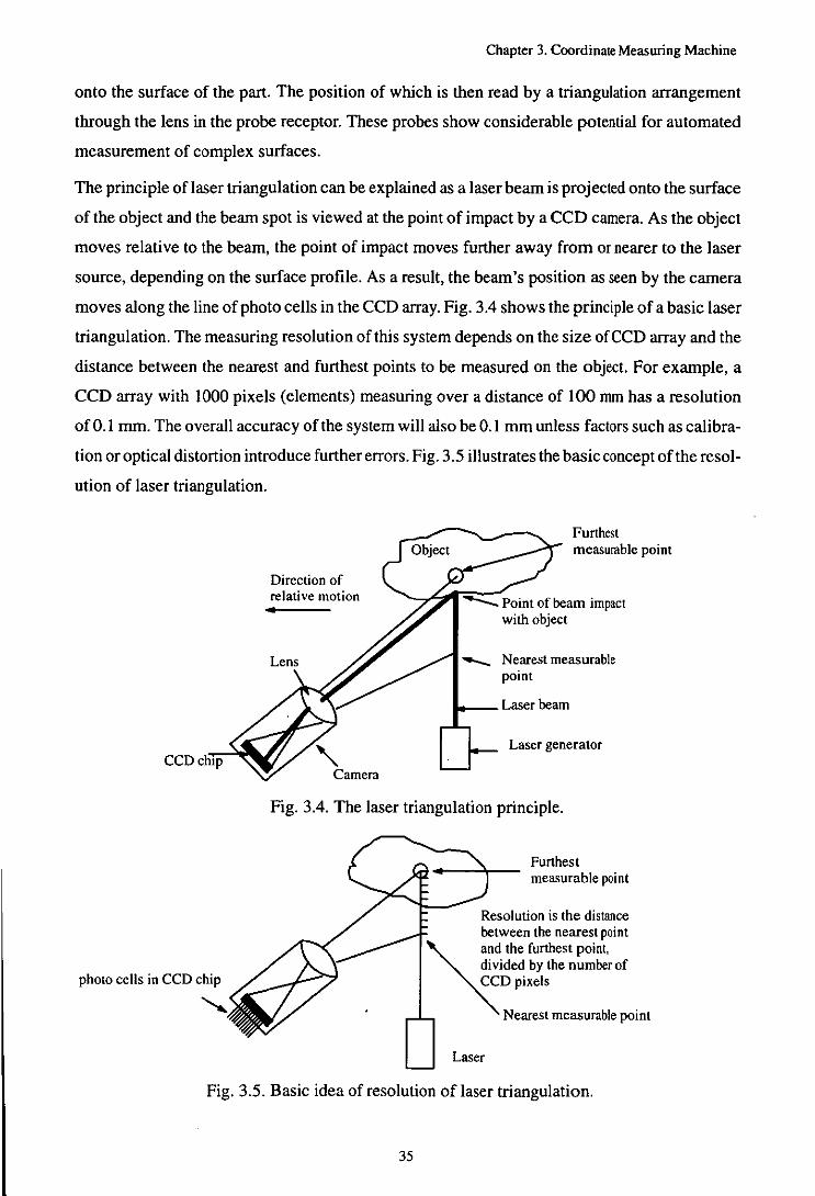
Chapter 3. Coordinate Measuring Machine
onto the surface of the part. The position of which is then read by a triangulation arrangement
through the lens in the probe receptor. These probes show considerable potential for automated
measurement of complex surfaces.
The principle of laser triangulation can be explained as a laser beam is projected onto the surface
of the object and the beam spot is viewed at the point of impact by a CCD camera. As the object
moves relative to the beam, the point of impact moves further away from or nearer to the laser
source, depending on the surface profile. As a result, the beam's position as seen by the camera
moves along the line of photo cells in the CCD array. Fig. 3.4 shows the principle of a basic laser
triangulation. The measuring resolution of this system depends on the size of CCD array and the
distance between the nearest and furthest points to be measured on the object. For example, a
CCD array with 1000 pixels (elements) measuring over a distance of 100 mm has a resolution
of 0.1 mm. The overall accuracy of the system will also be 0.1 mm unless factors such as calibra
tion or optical distortion introduce further errors. Fig. 3.5 illustrates the basic concept of the resol
ution of laser triangulation.
CCD chIp
photo cells in CCD chip
Direction of relative motion •
Furthest measurable point
'--~~r ____ :;;:::::::::-;;Point of beam impact with object
_ Nearest measurable point
.... __ Laser beam
Laser generator
Fig. 3.4. The laser triangulation principle.
Furthest measurable point
Resolution is the distance between the nearest point
~nd the furthest point,
divided by the number of CCDpixels
Nearest measurable point
Laser
Fig. 3.5. Basic idea of resolution of laser triangulation.
35
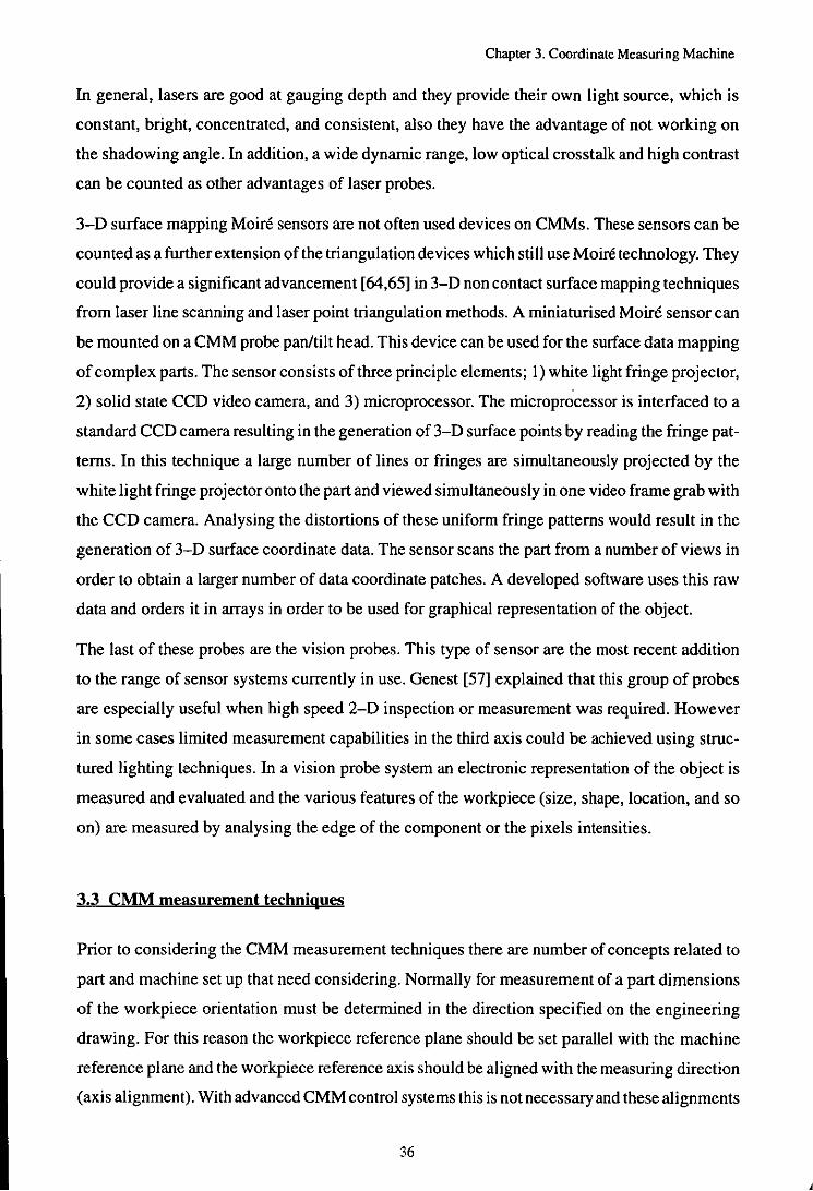
Chapter 3. Coordinate Measuring Machine
In general, lasers are good at gauging depth and they provide their own light source, which is
constant, bright, concentrated, and consistent, also they have the advantage of not working on
the shadowing angle. In addition, a wide dynamic range, low optical crosstalk and high contrast
can be counted as other advantages of laser probes.
3-D surface mapping Moire sensors are not often used devices on CMMs. These sensors can be
counted as a further extension of the triangulation devices which still use Moire technology. They
could provide a significant advancement [64,65] in 3-D non contact surface mapping techniques
from laser line scanning and laser point triangulation methods. A miniaturised Moire sensor can
be mounted on a CMM probe pan/tilt head. This device can be used for the surface data mapping
of complex parts. The sensor consists ofthree principle elements; I) white light fringe projector,
2) solid state CCD video camera, and 3) microprocessor. The microprocessor is interfaced to a
standard CCD camera resulting in the generation of 3-D surface points by reading the fringe pat
terns. In this technique a large number of lines or fringes are simultaneously projected by the
white light fringe projector onto the part and viewed simultaneously in one video frame grab with
the CCD camera. Analysing the distortions of these uniform fringe patterns would result in the
generation of 3-D surface coordinate data. The sensor scans the part from a number of views in
order to obtain a larger number of data coordinate patches. A developed software uses this raw
data and orders it in arrays in order to be used for graphical representation of the object.
The last of these probes are the vision probes. This type of sensor are the most recent addition
to the range of sensor systems currently in use. Genest [57] explained that this group of probes
are especially useful when high speed 2-D inspection or measurement was required. However
in some cases limited measurement capabilities in the third axis could be achieved using struc
tured lighting techniques. In a vision probe system an electronic representation of the object is
measured and evaluated and the various features of the workpiece (size, shape, location, and so
on) are measured by analysing the edge of the component or the pixels intensities.
3.3 CMM measurement techniques
Prior to considering the CMM measurement techniques there are number of concepts related to
part and machine set up that need considering. Normally for measurement of a part dimensions
of the workpiece orientation must be determined in the direction specified on the engineering
drawing. For this reason the workpiece reference plane should be set parallel with the machine
reference plane and the workpiece reference axis should be aligned with the measuring direction
(axis alignment). With advanced CMM control systems this is not necessary and these alignments
36

Chapter 3. Coordinate Measuring Machine
can be done by the CMM's computer system once the part coordinate system is established.
When a workpiece surface is measured using a probe, the coordinates of the probe centre are re
corded and these coordinates must be compensated for by offsetting the probe radius to determine
the actual workpiece dimensions. Currently CMMs are using data processing units and software
which perform probe radius compensation either in response to specific commands, or using an
automatic procedure which is based on the probe approach direction.
To measure a part it is necessary to establish a part coordinate system which is independent of
the machine coordinate system. This is recognised as the part coordinate system, and it can be
defined according to the drawing measurement datum surfaces and features on the workpiece.
The part coordinate system is established by levelling and aligning the part (workpiece) to the
measuring axis. It is important to set the part coordinate system that best suits the measurement
tasks required with reference to the drawing, because the measurement data is represented in the
coordinates in the part coordinate system.
3.3.1 Digitising. scanning and types of measurements by CMMs
CMMs can be arranged to scan or digitise the size and shape of an object or its contours by gather
ing raw data (in digital form) through sensors or probes. Digitising or scanning can be done from
a feature or a surface by digitising a point, a plane, or a cluster of points on a specified area. These
can either be measured as geometric shapes (flat surfaces as planes, holes as circles) or combined
from separate features into new geometric shapes (i.e., two intersecting planes define a line, etc.).
Digitising a point in space or a point on a surface of component by a CMM is basically achieved
by moving the sensing device (a probe) along the machine axes of travel until the probe contacts
the object. The coordinates of the point (probe centre) will be recorded in Cartesian form for fu
ture use. To digitise a line or a plane it is important to take the points as widely spread as possible.
Digitising can be divided into five groups; point by point, contouring, zig-zag digitising, one way
digitising and pencil mode (manual mode), fig 3.6 shows these tracing modes.
There are three general types of measurements for which CMMs are commonly used, geometric
measurement, contour measurement and surface measurement.
Geometric measurement deals with elements such as points, lines, planes, circles, cylinders,
cones, and spheres.
Contour or continuous path measurement has been defined as 2-D measurement of undefined
curves (profiles) where the probe measures at certain intervals by taking points on the surface
after each change of X and Y relative position in the machine axes. The measurement normally
37
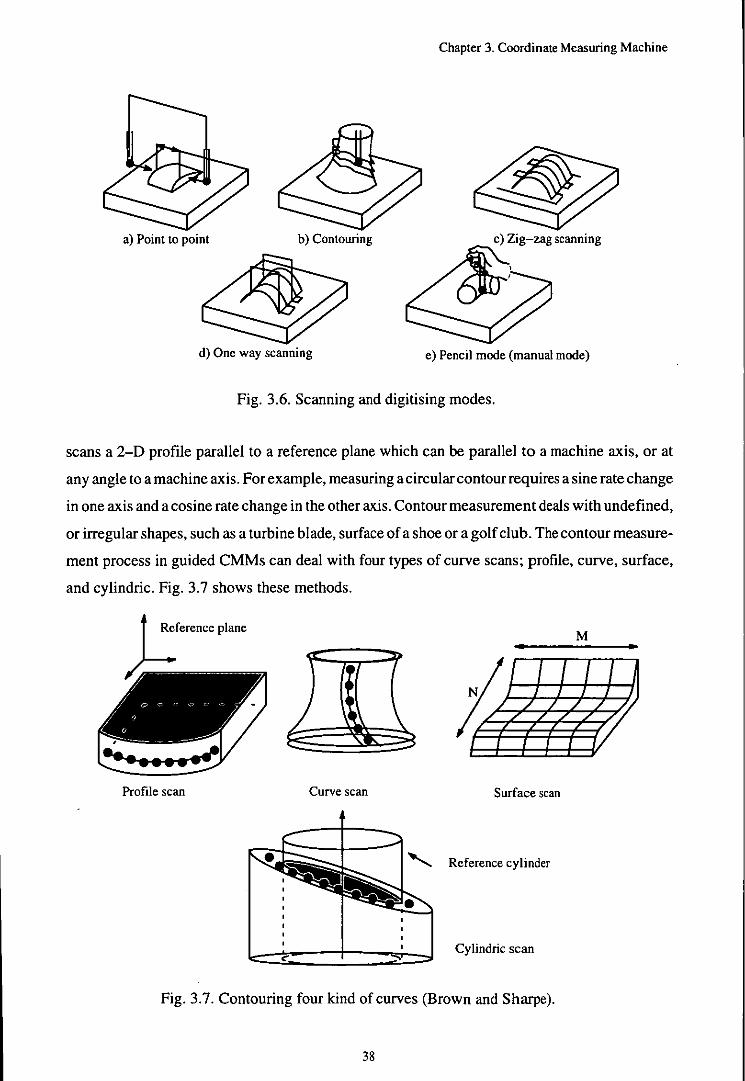
Chapter 3. Coordinate Measuring Machine
a) Point to point b) Contouring c) Zig-zag scanning
d) One way scanning e) Pencil mode (manual mode)
Fig. 3.6. Scanning and digitising modes.
scans a 2-D profile parallel to a reference plane which can be parallel to a machine axis, or at
any angle to a machine axis. For example, measuring a circular contour requires a sine rate change
in one axis and a cosine rate change in the other axis. Contour measurement deals with undefined,
or irregular shapes, such as a turbine blade, surface of a shoe or a golf club. The contour measure
ment process in guided CMMs can deal with four types of curve scans; profile, curve, surface,
and cylindric. Fig. 3.7 shows these methods.
M
\
Profile scan Curve scan Surface scan
Reference cylinder
Cylindric scan
Fig. 3.7. Contouring four kind of curves (Brown and Sharpe).
38
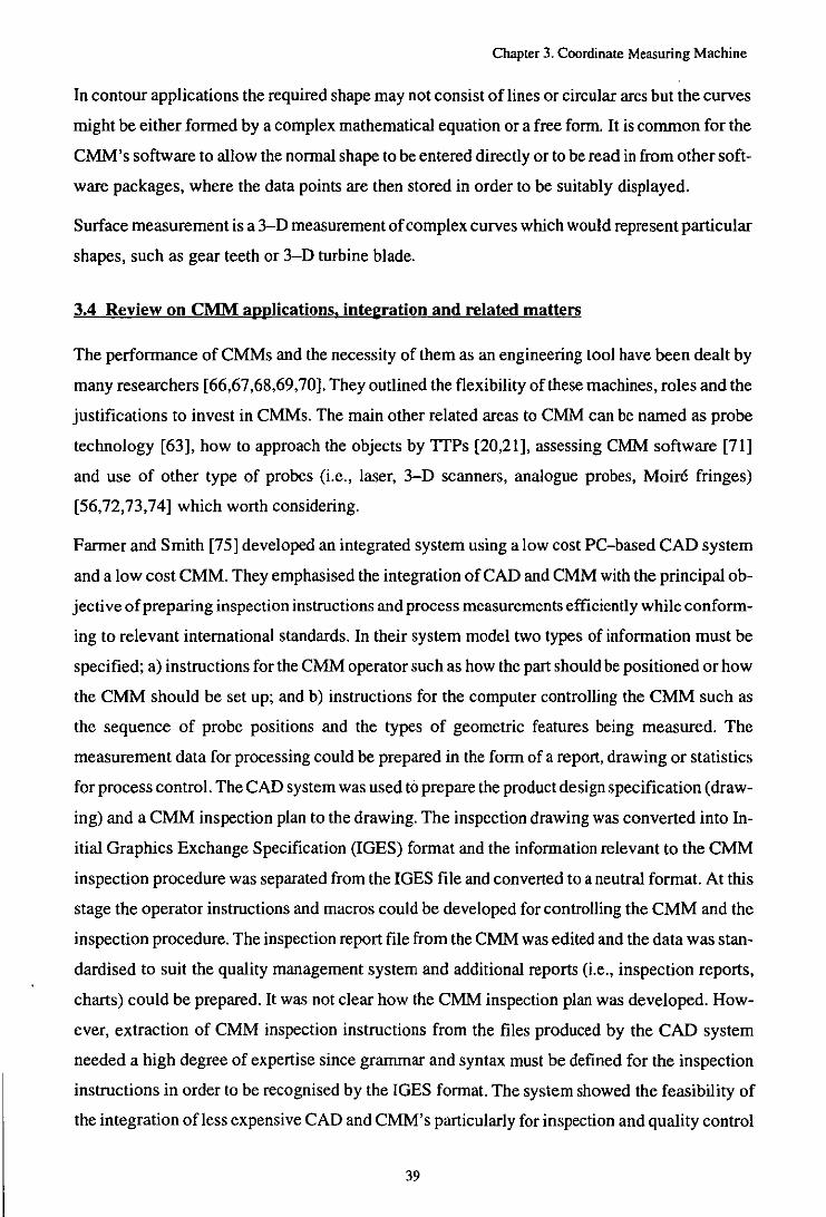
Chapter 3. Coordinate Measuring Machine
In contour applications the required shape may not consist of lines or circular arcs but the curves
might be either formed by a complex mathematical equation or a free form. It is common for the
CMM's software to allow the normal shape to be entered directly or to be read in from other soft
ware packages, where the data points are then stored in order to be suitably displayed.
Surface measurement is a 3-D measurement of complex curves which would represent particular
shapes, such as gear teeth or 3-D turbine blade.
3.4 Review on CMM applications. inte&ration and related matters
The performance of CMMs and the necessity of them as an engineering tool have been dealt by
many researchers [66,67,68,69,70). They outlined the flexibility of these machines, roles and the
justifications to invest in CMMs. The main other related areas to CMM can be named as probe
technology [63), how to approach the objects by TTPs [20,21), assessing CMM software [71)
and use of other type of probes (i.e., laser, 3-D scanners, analogue probes, Moire fringes)
[56,72,73,74) which worth considering.
Farmer and Smith [75) developed an integrated system using a low cost PC-based CAD system
and a low cost CMM. They emphasised the integration of CAD and CMM with the principal ob
jective of preparing inspection instructions and process measurements efficiently while conform
ing to relevant international standards. In their system model two types of information must be
specified; a) instructions for the CMM operator such as how the part should be positioned or how
the CMM should be set up; and b) instructions for the computer controlling the CMM such as
the sequence of probe positions and the types of geometric features being measured. The
measurement data for processing could be prepared in the form of a report, drawing or statistics
for process control. The CAD system was used to prepare the product design specification (draw
ing) and a CMM inspection plan to the drawing. The inspection drawing was converted into In
itial Graphics Exchange Specification (IGES) format and the information relevant to the CMM
inspection procedure was separated from the IGES file and converted to a neutral format. At this
stage the operator instructions and macros could be developed for controlling the CMM and the
inspection procedure. The inspection report file from the CMM was edited and the data was stan
dardised to suit the quality management system and additional reports (i.e., inspection reports,
charts) could be prepared. It was not clear how the CMM inspection plan was developed. How
ever, extraction of CMM inspection instructions from the files produced by the CAD system
needed a high degree of expertise since grammar and syntax must be defined for the inspection
instructions in order to be recognised by the rGES format. The system showed the feasibility of
the integration ofless expensive CAD and CMM's particularly for inspection and quality control
39

Chapter 3. Coordinate Measuring Machine
for manufacturers. However, their system did not consider automatic inspection of features and
it required continuous user intervention.
Pahk et al. [76] developed a CMM and CAD inspection system for integrated mold manufactur
ing. The system was capable of measuring sculptured surfaces with some basic features such as;
holes, slots and bosses. The features could be chosen in a CAD section in which inspection plan
ning for each feature would be created. The output of the planning was the machine code for a
specific CNC CMM. Error analyses arrangements in the CAD system allowed compensation to
be made on received data from CMM and the evaluated errors would be graphically displayed.
A least squares technique was used for error evaluation of basic features such as flatness, square
ness and parallelism. Other error algorithm have been developed to calculate form and offset er
rors which were involved in tilting or translation of the sculptured surfaces on the mold plate.
The system was based on the existence of the objects' CAD model which needed further research
for both automatic inspection of the features on the designed model and to make the system appli
cable to complex products.
Oh et al. [77] researched on the use of CMM in reverse engineering, the process of making a part
from an existing part rather than from a drawing.
They discussed five major steps of the reverse engineering cycle which were;
I). Measure and digitise the original part.
2). Transmit the CMM data to a CAD system.
3). Transforming the point data to a CAD model.
4). Generate NC tool path.
5). Produce a new part using the path programme.
Kwok and Eagle [78] discussed two major applications of reverse engineering by use of a CMM.
The first application was creating CAD models of surfaces that are based on appearance rather
than on engineering requirements examples such as shampoo bottles and automobile dashboards
which are designed largely for their pleasing appearance, the CAD models of these crafted proto
types would be created by CMM digitising. The second application as mentioned earlier was to
produce drawings of existing parts when the original design data were unavailable. The main
similarity of these two studies [77,78,] to this work is in the process of creating the object on the
CAD system by a CMM.
Sarkar and Menq [15] considered schemes for scanning compound surfaces by a touch probe
CMM. Scanning compound surfaces required two important concepts; a) definition of the bound-
40
Chapter 3. Coordinate Measuring Machine
aries or character lines, and b) definition of regions bounded by the character lines. The boundary
points could be digitised manually, by the use of vision techniques, or by enhanced CMM scan
ning procedures to define the character lines. The main concept was the division of the compound
surface into a number of regions by the use of the character lines. The character lines signify the
change in the surface shape which means each region will have no an apparent shape change. The
position of the character lines could be visually detected and manually digitised or they could be
determined by edge operators. However, none of these methods could be fully automated without
manual intervention for a very general compound surface due to the degree of complexity. Also,
for complicated 3-D objects with undercuts, scanning is difficult using a CMM without reloca
tion or orientation.
The CMM probe technology and errors associated with them have been studied by many re
searchers, notably Reid [63] examined the fundamental requirements for the technology
employed in a CMM probe sensor. He discussed that the principle of operation of Strain Guage
Probes (SGPs) which eliminates the measurement uncertainty associated with lobbing by effec
tively triggering the probe at a constant force in all probing directions.
Smith [20] investigated the errors associated with variation in the angle of contact of a TTP. The
error of a TIP reaches its minimum when the probe approaches the surface in the normal direc
tion. Butler [21] researched into the nature of probe errors and factors that influence their per
formance with a proposed method of verifying the probe performance. Although the use of a SGP
may improve probing for the majority of industrial applications, the developed probing strategy
in this work supports the work of Smith and Butler [20,21] and minimised the errors associated
with TTPs.
Cox [71] discussed methods for assessing and comparing CMM software qUality. The methodol
ogies for CMM software testing could be classified as:- i) correctness proving, the application
of classical mathematical proving methods to metrology software, ii) self assessment using math
ematical properties, in order to confirm that the computed solutions satisfies the original math
ematical problem statement, and iii) black box testing through the use of reference data sets (soft
guages). The reference data sets are synthesized data sets that mimic actual measurement data.
A good software should be consisted of: a) a rigid mathematical basis, b) good numerical analy
sis, c) careful algorithm design, and d) sound software implementation.
There is an increase in use of non contact probes with CMMs, Goh et al. [72] discussed the main
advantages of non contact inspection and methods adaptable for the dimensional inspection of
engineering components by the use of a compact solid state laser triangulation sensor on a CMM.
41

Chapter 3. Coordinate Measuring Machine
They were encouraged not to use a TIP due their limitations, such as possible local deformation,
overshooting of the probe, critical surface fmishes might be marred and slow speed of the
measurement. Renishaw [79] developed a non contact probing system for the use with CMM to
allow high speed scanning. The system used the triangulation principle within a laser light beam
which was focused to a spot by the optics contained with the probe. The spot was typically fo
cused between 20 and 100 mm from the probe. Since the majority of engineering materials are
non-perfect reflectors, the surface would reflect the laser light in multiple directions. However,
the system was able to operate with a portion of the scattered light which was focused onto a light
sensitive detector.
Laser applications are rapidly increasing in the area of measurement, Bradley et al. [73]
employed a 3-D laser scanning on a Mitutoya BHM 710 CMM to digitise object surfaces. The
scanner operation was controlled on a tenninal through a hierarchical menu. The scanner unit
would move within the 3-D work envelop by the CMM and multiple passes could be made at
any depth (providing the surface was within the scanners depth of field) across the prototype sur
face until satisfactory digitisation could be achieved. The servo motor position encoders of the
CMM kept updating the scanner computer during data collection. The quoted accuracy of ± 0.05
mm could theoretically be increased by reducing the depth of field from the current 80.0 to 40.0
mm. The process would be used to reconstruct regions of the laser scanned object, which could
be represented by a sub-set of the family of quadric surfaces, namely planes, cylinders, cones
and spheres. Although the laser scanning accuracy was not as high as a CMM, it would be ap
propriate for many reverse engineering tasks and rapid prototyping of multi patch models.
Although there are some benefits with the use of non contact probes or scanners, there are some
drawbacks with using them such as, high cost or complexity and less flexibility. However, they
still attract specific applications in industry.
3.5 Factors affecting CMM performance
The CMM performance and its accuracy will be affected by many error sources which can be
grouped into three categories: i) design errors, ii) environmental errors, and iii) operating errors.
An evaluation of these errors will give the overall machine performance. Genest [57] believed
that most errors in CMMs were of systematic kind, initiated from machine set -up and operating
conditions rather than random. Therefore a series of initial considerations should be given when
a CMM is to be used to give a high level of performance, the CMM should be placed in a suitable
environment with adequate safeguards and protection for error free operation.
42

Chapter 3. Coordinate Measuring Machine
There are many sources of geometric inaccuracy in a three axis CMM which are; roll, pitch, yaw,
scale error (linear positioning), straightness, and squareness. To ensure volumetric accuracy (ex
plain later), every one of these factors must be tested. However, the majority of mechanical errors
in the CMM may be refIned using computer control and some of the others may automatically
be compensated for by the use of powerful software algorithms during measurements [57].
Workpiece errors and probe workpiece interaction would be named as error sources which could
be belong to the mechanical characteristics of the workpiece materials, examples of which could
be hardness and roughness.
3.5.1 Geometric and kinematic errors on CMMs
In general it is impossible to manufacture a mechanically perfect machine, however it is import
ant to be able to analyse the geometric errors associated with individual elements and to determine
their effects on the machine's measurement accuracy. Geometric and kinematic error analysis
tends to be of concern for the manufacturers of CMMs rather than the end user who is only inter
ested in the accuracy to which he can measure using the machine. However, the geometric error
of a CMM is one of the major sources contributing to the inaccuracy of a measured workpiece.
The geometric error of a CMM is the error which is produced at the probe stylus due to dimen
sional and form errors of the elements of its kinematic linkage system, and the angular and posi
tional misalignments between them. The accuracy of CMMs also depends on the accuracy of the
position transducers and on the linear and rotary moving axes. Elshennawy [2] explained that
geometric accuracy of the machine could be affected by the following factors,
i) Errors in the form of different machine component shapes such as tables, guideways, etc.
ii) Mechanical wear of linkages and joints which introduce undesirable effects such as lack of
straightness and squareness, inadequate motion, etc.
iii) Thermally induced errors due to variations in the operating environment which would cause
structural changes.
iv) Weight deformations caused by the weight of machine structure or the part being machined
or measured.
v) Errors in the control or measuring system which could be thermal, mechanical or electrical
in nature.
3.5.2 Probe error sources within a kinematic/resistive probe
The electrically switching kinematic 3-D TIP was fIrst available in 1972 and the principle of
operation has not changed since then. Reid [60] explained that the potential probe error sources
43
Chapter 3. Coordinate Measuring Machine
within kinematic/resistive TIPs fall into two main types: random errors, and systematic errors
which are generally application sensitive and could be either eliminated or minimised in practice.
The only random error source which could be associated with kinematic/resistive TIPs is the uni
directional repeatability which is present in all measurements taken. The repeatability of a probe
is the competence of the probe to trigger at the same point each time and normally quoted statisti
cally with a 95 per cent confidence level. The repeatability error of kinematic/resistive TIPs
being typically less than 0.5 !lm. This is not likely to be the major source of measurement error
on a CMM, however, its presence should be considered when appraising the measuring perfor
mance of any CMM or a probing system.
With kinematic/resistive TIPs systematic errors can be grouped into two main potential sources:
pre travel variation and hysteresis. As mentioned before the degree of presence of these potential
error sources are significantly influenced by the datuming and measuring techniques employed,
the model of probe used, and the type of feature being measured.
Directional variation in probe pre travel may be as small as ± 1 !lm if a good datuming technique
is employed. The effective tip diameter of a probe (stylus tip) would be calculated by the CMM
software and is applied to each point taken by the probe to give the true position of the inspection
surface.
There are methods suggested by the standard bodies to establish the possible errors contributing
to the total system measuring error by the probing system. A method is suggested by ANSIJ
ASME B89 standard for a probing system which lays out a performance test in order to establish
the possible errors contributing to total system measuring error. The test involves taking 49 probe
points over the surface of a test sphere using three different stylus configurations.
There are a number of considerations recommended [80,81,82] to optimise the use of the probe:
i) Keep the stylus configurations as short and rigid as possible.
ii) Keep the probe trigger force (if applicable) as low as possible whilst ensuring reliable probe
operation.
iii) Datum the probe in the directions it will be used by taking at least five equispaced points
spread over the surface of the datum sphere.
iv) When measuring a feature with multiple points, take points sequentially around the feature,
always trying to take more points than the minimum required.
v) TIP accuracy varies as the stylus orientation varies. The best results can be obtained from a
CMM by always approaching perpendicular to the part's surface and to use a large portion of the
44
Chapter 3. Coordinate Measuring Machine
feature.
vi) Follow the suggested measurement procedure by the CMMs and TIPs manufacturers.
vii) Ensure the probe holder is placed correctly to the machines' quill.
viii) Any time the probe has been removed and reinserted into the CMM, the qualification must
be re executed, because the probe can never be mounted identically and there are some inconsis
tencies on the probe stylus.
Probe hysteresis is often an overlooked systematic error which can be present in all types of probe
design. It could occur as a direct consequence of the direction of the previous trigger and reseat
and could be thought of as being backlash similar to other mechanical systems. Hysteresis error
is generally of the same order of magnitude as probe repeatability and it is directly proportional
to the stylus length and the trigger force in a TTP [60].
3.5.3 Errors due to environmental effects
Error due to environmental effects would generate a continuous error in the CMM and unless a
recommended environment is prepared these factors are difficult to control. The environmental
effects could be caused by;
Temperature. A stable temperature is necessary to avoid thermal distortion. This is particularly
important if alloy or plastic components are to be measured. Specific operating temperature stan
dards have not been established. One of the environmental requirements is the temperature at the
location of the measuring equipment, for example the temperature in a laboratory doing interfer
ometer calibration for 2 flm and for CMM to 10 flm accuracy should be held to ± 1120 oF. The
nominal temperature should be 68 of (20 ± 1°C) to eliminate one of the correction factors when
comparing results directly with National Bureau of Standards (NBS) [83].
Vibration. Many CMMs are mounted on anti vibration mounts; however, it is still important to
minimise vibration in the vicinity of the machine. Some of the common sources of vibration are
air compressors, punch presses, large mills and shapers (common machines in a workshops), etc.
Contamination. In order to keep maintenance to a minimum it is advisable to select a suitable
site which is relatively free from contamination by oil, swarf, dust, humidity etc. The compressed
air supply to the machine should be dry and oil free.
Electrical interference. The electronic desk should be supplied from a power line which is iso
lated from power cables supplying electrical equipment which may cause large voltage fluctu
ations or interference pulses.
Handling. Avoid touching the ground surfaces of columns or any other bearing ways with bare
45

Chapter 3. Coordinate Measuring Machine
hands. If it is necessary to move the machine manually, it is advisable to hold the Z column by
the upper part of the probe mount [57].
3.5.4 Yolumetric accuracy
As CMMs begin to be used to measure more complex parts, linear accuracy may not be sufficient
to guaranty the level of measurement performance required. Therefore it is important to evaluate
its volumetric accuracy, which is the performance of the CMM accuracy at any point within its
three dimensional working envelope.
The maximum permitted error for volumetric accuracy is given by [84];
Volumetric accuracy u = A +..Bf- pm ..... 3.1
Where U is the maximum permitted error (volumetric accuracy) in measuring a known length
of L millimetres in any position on the machine. A, B, and C are constants given in the specifica
tion of the particular CMM. BS6808 requires that the U shall be stated at a confidence level not
less than 95 per cent. For example a CMM model with repeatability of 0.001 mm and the volumet
ric accuracy given as 2.8 + 3UlOOO f.lm, the uncertainty on measuring a length is 2.8 f.lm plus
an additional amount of 3 f.lm per metre of the measured length [84]. There are practical ways
such as; laser measurement systems and Machine Checking Gauge (MCG) tests for determining
volumetric accuracy of a CMM by the user. Dimensions and tolerance limits would be generally
referred by implication to a theoretical temperature of 20° C.
3.6 The CMM systems used for this work
The two CMMs used for this project were of a moving bridge type which employ three movable
components moving along mutually linear perpendicular guideways. The probe is attached via
fittings to the vertical component. Fig. 3.8(a and b) show a Ferranti Merlin and a Micro Xcel Tesa
CMM from the Brown and Sharpe Company.
The initial set of primary tests were undertaken on a Ferranti Merlin MKll series 750 CMM with
a Hewlett Packard 9000 Series 300 computer control system [14]. The machine operates under
full 3-axis computer numerical control (CNC) using the CMM initialise software named
DCC-3l5. This software enables various standard measuring routines and calculations to be per
formed. The machine is of a gantry configuration which enables a 750 x 750 x 500 (mm) envelope
to be measured. The machine has an linear accuracy of 0.005 (mm) and a repeatability of 0.02
(mm).
The measuring head used for this work was a standard Renishaw PH9 motorised probe head.
Through the CMM software the head allows for 20 probe orientation at 7.5 degree increments.
46

Chapter 3. Coordinate Measuring Machine
The touch probing was achieved using standard 0.3 mm, 1.0 mm, and 2.0 mm diameter spherical
ruby tips.
During the course of the project a new CMM was purchased by the University which had the fol
lowing advantages over the Ferranti Merlin. It allows the use of hundreds of probe orientations
and generates direction vectors (IJK) of the measuring points. The machine is a bench type (425
Kg.), low cost and high performance measuring machine with an mM compatible computer sys
tem which runs on SCO Xenix operating system. The machine enables users to toggle effortlessly
between manual and DCC operation mode and operates under fu1l3-axis CNC with an initialise
software named Micro-Measure-4 (MM4). The machine has a 457 x 508 x 406 (mm) measuring
envelope with a linear accuracy of 0.005 (mm), a repeatability of 0.003 (mm), and a volumetric
performance of3 + 3L/1000. The measuring head used for it was a standard Renishaw PH9 which
allows for 700 probe orientations at 7.5 degree increments [82].
It was therefore decided to use the Tesa for the majority of the tests and the early developed system
on the Ferranti was transferred to the Tesa CMM.
3.7 Future developments of CMMs
The future development ofCMMs can be divided into: I) software development and, 2) hardware
development. The software development of a CMM needs to handle a variety of processes in real
time with robust algorithms, a wide range of functions, a good interfacing system with CAD and
CAM environments, and the possible need for handling vision data. A logical link to better shar
ing of information is needed to interface between the design data and the inspection data. The
link between CAD and CMM allows information to be passed between the two systems, this inter
face is usually unidirectional from the CAD system to the CMM however, multidirectional links
will be needed in the future. In addition, the CMM controllers of the future should have the capa
bility of not only handling procedure commands (where the CMMs are asked to measure) but also
the process geometry commands (where the CMMs will understand geometry commands and
feature description commands) [85]. The connection of3-D CMM to NC and CNC systems with
off-unit programming opens possibilities for CIM with flexible measuring inspection to develop
automatic probe changing systems without the requirement of subsequent recalibration [67].
An important part of the software development concerns interfacing which enables translating
data between the systems. In order to advance and accelerate the production cycle of a part from
design to manufacture it is important to allow part data to flow quickly and accurately between
all those processes involved. There are a few such data interchange standards/methods currently
available such as IOES, PDES, STEP, and DMIS [38,86]. DMIS has been specifically developed
47
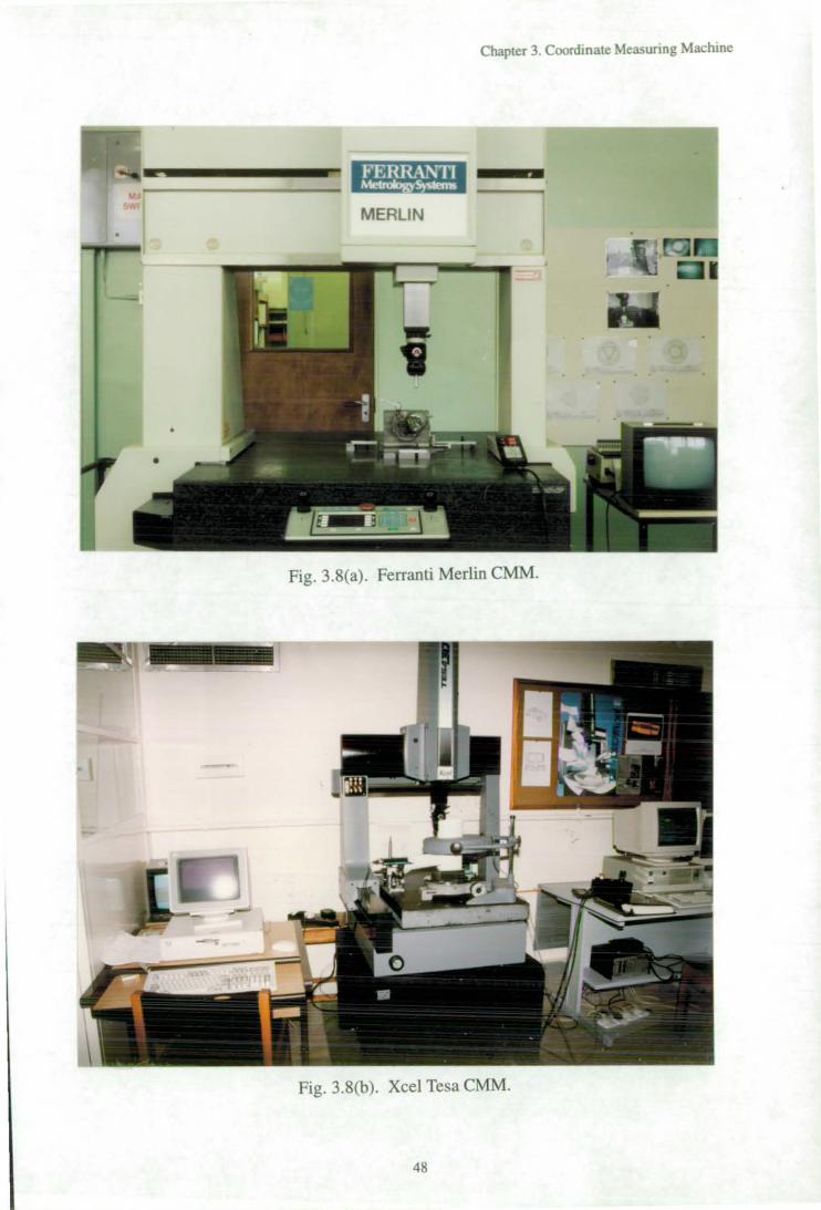
FERRANTI ~
MERLIN
Chapter 3. Coordinate Measuring Machine
_
Fig. 3.8(a). Ferranti Merlin CMM.
Fig. 3.8(b). Xcel Tesa CMM.
48
~--------- - -
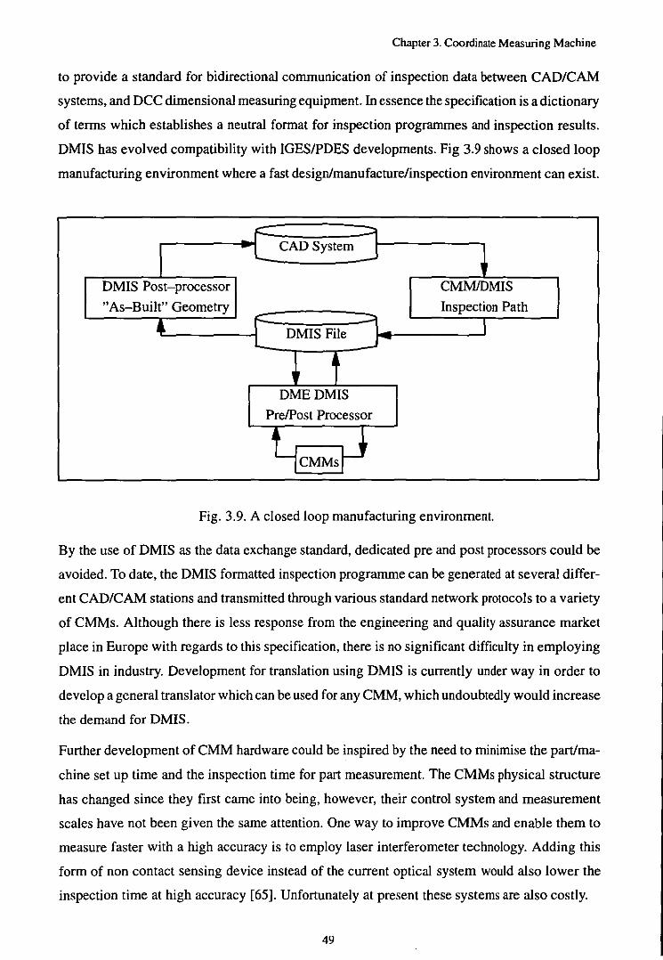
Chapter 3. Coordinate Measuring Machine
to provide a standard for bidirectional communication of inspection data between CAD/CAM
systems, and DCC dimensional measuring equipment. In essence the specification is a dictionary
of terms which establishes a neutral format for inspection programmes and inspection results.
DMIS has evolved compatibility with IGESIPDES developments. Fig 3.9 shows a closed loop
manufacturing environment where a fast design/manufacture/inspection environment can exist.
~f :==, CAD System ·L j
DMIS Post-processor CMMlDMIS
"As-Built" Geometry Inspection Path .. f L DMIS File L J
DMEDMIS
PrelPost Processor
~CMMS~ Fig. 3.9. A closed loop manufacturing environment.
By the use of DMIS as the data exchange standard, dedicated pre and post processors could be
avoided. To date, the DMIS formatted inspection programme can be generated at several differ~
ent CAD/CAM stations and transmitted through various standard network protocols to a variety
of CMMs. Although there is less response from the engineering and quality assurance market
place in Europe with regards to this specification, there is no significant difficulty in employing
DMIS in industry. Development for translation using DMIS is currently under way in order to
develop a general translator which can be used for any CMM, which undoubtedly would increase
the demand for DMIS.
Further development of CMM hardware could be inspired by the need to minimise the partlma~
chine set up time and the inspection time for part measurement. The CMMs physical structure
has changed since they first came into being, however, their control system and measurement
scales have not been given the same attention. One way to improve CMMs and enable them to
measure faster with a high accuracy is to employ laser interferometer technology. Adding this
form of non contact sensing device instead of the current optical system would also lower the
inspection time at high accuracy [65]. Unfortunately at present these systems are also costly.
49

Chapter 4. Feature detection using machine vision and a CMM
CHAPTER 4
FEATURE DETECTION USING MACHINE VISION AND A CMM
4.0 Introduction
Data collection of 3-D coordinate information from sculptured surfaces has been achieved by
the use of contact and non contact techniques, however, the use of these methods is still causing
some difficulties. When using a contact technique collection of data can be arranged by touching
a point at a time which is a slow process. The specification of features for sculptured parts is still
uncertain and generally lines or grids are marked onto the surface to identify features or patches.
More sophisticated methods are required to enable this process be done faster. This feature detec
tion and measurement strategy will include a systematic method for presenting the features in
order for them to be easily identified, sorting of the detected features, development of an optimal
procedure to measure features, and design of a strategy for the probe selection in order to mini
mise the probing error.
Prior to inspecting the surface features, their locations need to be identified and for special cases
when the surfaces could have many features, a fast detection and reliable method is required. One
possible method is to employ the use of a machine vision to identify the locations of the features.
Because it is difficult to separate features on a sculptured part, they need to be enhanced by mark
ing in order for them to be easily identified. The 2-D vision system used then determines the posi
tion of each feature which is treated as if it was on a similar horizontal plane, a set of algorithms
and procedures were designed to analyse the problem.
For this research the selected objects were golf balls which are special cases of multi faceted fea
ture parts albeit positioned around a regular object sphere and which also gives the opportunity
for measuring multiple facets. For simple balls the dimple shape would be constant (one dimple
shape repeated around the whole ball), whereas complex balls can have as many as eleven dimple
sizes. It is apparent that there are no generic solutions for automated feature identification and
detection and, one way of developing methods is by investigating special cases in order to learn
rules and methods which can be applied elsewhere (e.g., shoe last inspection etc.). Jones and
Mitchell [87,88] investigated and developed generic methods through studying feature based de
sign of specific sculptured products, they concentrated in investigating solutions for one product
from which methods and rules have been developed and applied elsewhere.
4.1 Golf balls
Although many books have been written about the history of golf, the true origin of the game has
yet to be decided. The playing of a game resembling golf is evident in Dutch illustrations [89,90]
50

Chapter 4. Feature detection using machine vision and a CMM
dating as far back as 1296. However historians agree that it was the Scots who taught the world
to play golf. What it is certain is that the game has existed for at least 500 years. This is known
because an Act of Parliament dated 6 March, 1457 [90] clearly states that James IT of Scotland
had football and golf banned because their popularity strongly interfered with archery practice,
important in those days for the defence of the realm against the English warriors.
A monopoly for ball manufacture was given in 1618 by James VI of Scotland to James Melvill
and his associate for a period of2l years [90] and referred to balls which were made from leather
and stuffed with feathers. However feathery balls started to be superseded by the innovation of
a new ball made from Gutta Percha in 1848. The Gutta Percha ball reigned supreme for almost
55 years, until it was superseded by the HaskeIl ball in 1902. The modem golf ball is a direct de
scendant of the HaskeIl rubber cored ball which brought improved performance and greater in
terest in the game. Today wound balls make up 20 per cent of the market with solid two piece
and one piece balls the remainder. Manufacturers constantly strive to produce balls which go
further etc. and, in order to maintain standards and control performance the twin governing
bodies of the game, the Royal and Ancient (R&A) Golf Club and the United State of Golf Associ
ation (USGA), have placed a set of restrictions on ball design [91].
a. Weight
The weight of the ball shall not be greater than 1.620 ounces avoirdupois (45.93 gm).
b. Size
The diameter of the ball shall be not less than 1.680 inches (42.67 mm). This specification will
be satisfied if, under its own weight, a ball falls through a 1.680 inches diameter ring guage in
fewer than 25 out of lOO randomly selected positions, in at a temperature of23 ±l cC.
c. Spherical symmetry
The ball must not be designed, manufactured or intentionally modified to have flight properties
which differ from those of spherically symmetrical ball.
The ball performance specifications outlined by the Rules of Golf [91] is that each ball type will
be tested using 20 pairs of that type. One ball of each pair will be launched spinning about one
specified axis; the other ball of each pair will be launched spinning about a different, but also
specified axis. Differences in carry and time of flight between the two balls of each pair will be
recorded. If the mean ofthe differences in carry is greaterthan 3.0 yards, and that value is signifi
cant at the 5 per cent level, or if the mean of the differences in time of flight is greater than 0.20
seconds, and that value is significant at the 5 per cent level, the ball type will not conform to the
Rules of Golf.
51
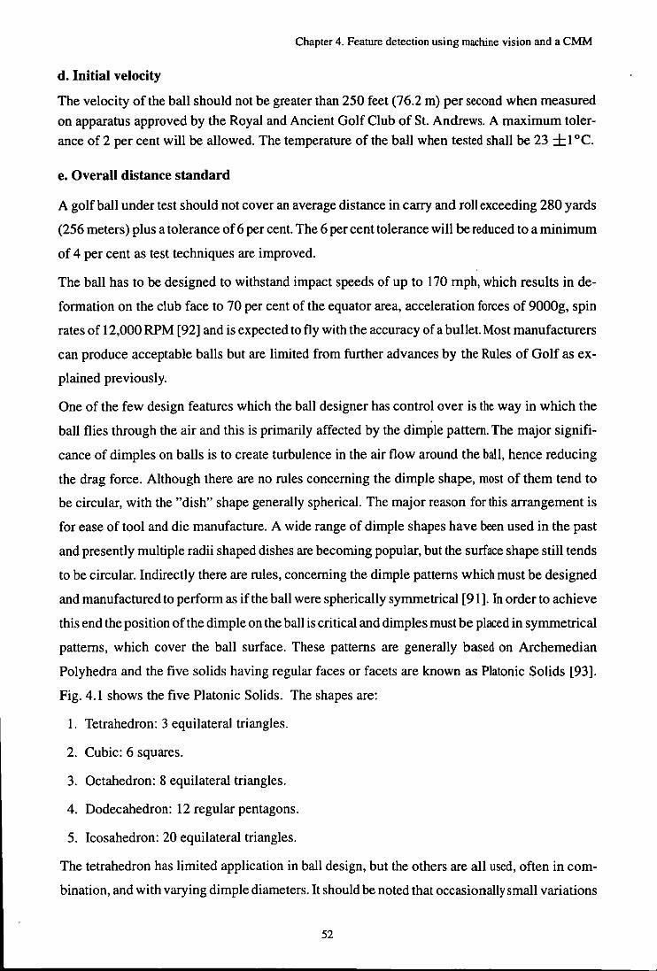
Chapter 4. Feature detection using machine vision and a CMM
d. Initial velocity
The velocity of the ball should not be greater than 250 feet (76.2 m) per second when measured
on apparatus approved by the Royal and Ancient Golf Club of St. Andrews. A maximum toler
ance of 2 per cent will be allowed. The temperature of the ball when tested shall be 23 ±l 0c.
e. Overall distance standard
A golf ball under test should not cover an average distance in carry and roll exceeding 280 yards
(256 meters) plus a tolerance of 6 per cent. The 6 per cent tolerance will be reduced to a minimum
of 4 per cent as test techniques are improved.
The ball has to be designed to withstand impact speeds of up to 170 mph, which results in de
formation on the club face to 70 per cent of the equator area, acceleration forces of 9000g, spin
rates of 12,000 RPM [92] and is expected to fly with the accuracy ofa bullet. Most manufacturers
can produce acceptable balls but are limited from further advances by the Rules of Golf as ex
plained previously.
One of the few design features which the ball designer has control over is the way in which the
ball flies through the air and this is primarily affected by the dimple pattern. The major signifi
cance of dimples on balls is to create turbulence in the air flow around the ball, hence reducing
the drag force. Although there are no rules concerning the dimple shape, most of them tend to
be circular, with the "dish" shape generally spherical. The major reason for this arrangement is
for ease of tool and die manufacture. A wide range of dimple shapes have been used in the past
and presently mUltiple radii shaped dishes are becoming popular, but the surface shape still tends
to be circular. Indirectly there are rules, concerning the dimple patterns which must be designed
and manufactured to perform as if the ball were spherically symmetrical [91]. In order to achieve
this end the position of the dimple on the ball is critical and dimples must be placed in symmetrical
patterns, which cover the ball surface. These patterns are generally based on Archemedian
Polyhedra and the five solids having regular faces or facets are known as Platonic Solids [93].
Fig. 4.1 shows the five Platonic Solids. The shapes are:
I. Tetrahedron: 3 equilateral triangles.
2. Cubic: 6 squares.
3. Octahedron: 8 equilateral triangles.
4. Dodecahedron: 12 regular pentagons.
5. Icosahedron: 20 equilateral triangles.
The tetrahedron has limited application in ball design, but the others are all used, often in com
bination, and with varying dimple diameters. It should be noted that occasionally small variations
52
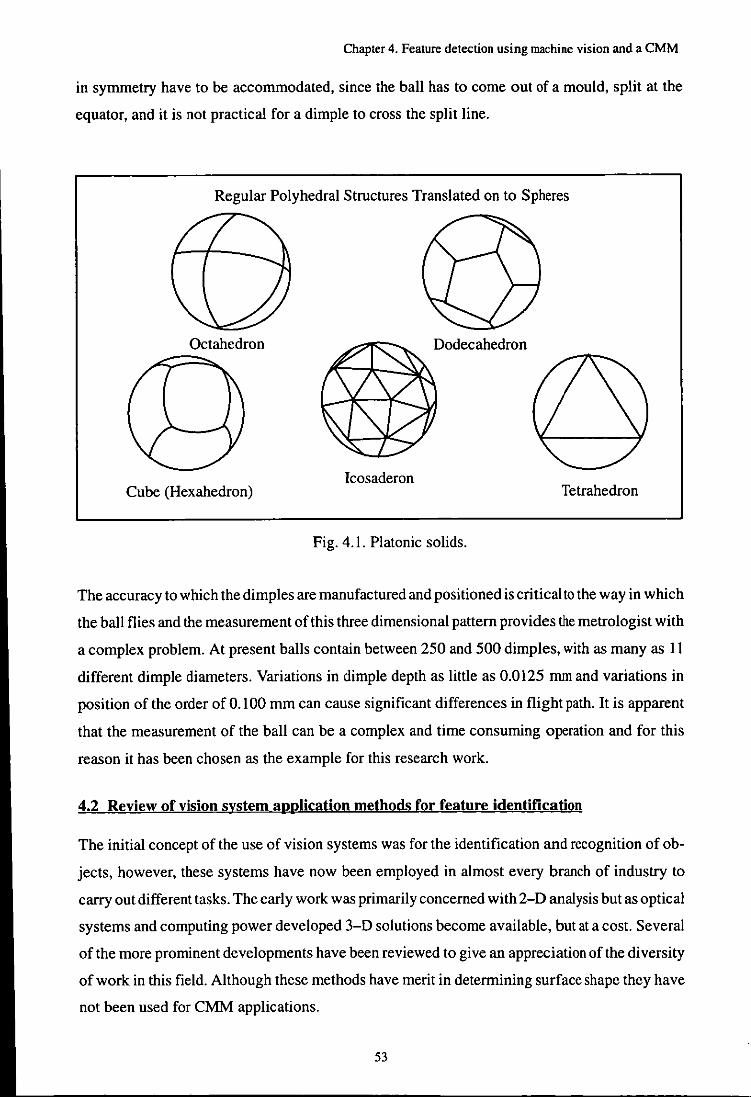
Chapter 4. Feature detection using machine vision and a CMM
in symmetry have to be accommodated, since the ball has to come out of a mould, split at the
equator, and it is not practical for a dimple to cross the split line.
Regular Polyhedral Structures Translated on to Spheres
Octahedron
Icosaderon Cube (Hexahedron) Tetrahedron
Fig. 4.1. Platonic solids.
The accuracy to which the dimples are manufactured and positioned is critical to the way in which
the ball flies and the measurement of this three dimensional pattern provides the metrologist with
a complex problem. At present balls contain between 250 and 500 dimples, with as many as 11
different dimple diameters. Variations in dimple depth as little as 0.0125 mm and variations in
position of the order of 0.100 mm can cause significant differences in flight path. It is apparent
that the measurement of the ball can be a complex and time consuming operation and for this
reason it has been chosen as the example for this research work.
4.2 Review of vision system application methods for feature identification
The initial concept of the use of vision systems was for the identification and recognition of ob
jects, however, these systems have now been employed in almost every branch of industry to
carry out different tasks. The early work was primarily concerned with 2-D analysis but as optical
systems and computing power developed 3-D solutions become available, but at a cost. Several
of the more prominent developments have been reviewed to give an appreciation of the diversity
of work in this field. Although these methods have merit in determining surface shape they have
not been used for CMM applications.
53
Chapter 4. Feature detection using machine vision and a CMM
Blake et al. [94,49] developed a method of active range sensing for the detection of features or
objects, using the trinocular stereo method which employs two projectors each of which projects
a pattern of stripes onto the object. Although this system could detect the general shape of the
object, it could not equally process the image patterns on each side of the object which resulted
in loosing some of the data at the weaker side (the side opposite to the line of camera projection).
This was caused by placing one camera at an angle to the projection axis of the light stripes. There
was also a need for careful alignment of the patterns projector with the camera in order to avoid
the computational expense of constraint propagation and the problem of ambiguity of the node
positions (intersections of the light stripes). It was claimed that the system worked well in a lab
oratory environment over a working volume of a 50 mm cube with a depth of resolution of around
0.2 mm, however, there appears to be no significant industrial application of this method.
Celenk and Bachnak [95] designed a stereo vision method for 3-D information extraction and
surface reconstruction of objects in a robot workspace. They used a number of camera pairs to
view the objects. The camera pairs were defined with respect to a coordinate system datum and
placed at the maximum allowable distance from the datum in order to use the minimum number
of cameras that cover the workspace entirely. The system requirement was; a knowledge of the
common area between the left and right images, relationship between image planes and scene
domain, and the internal and external parameters of the system. The system was required to input
an initial guess (prior knowledge) for the surface in order to be able to reconstruct the surface
accurately. The degree of accuracy, speed of camera calibration or the matching procedure was
not stated. Although this approach would have potential for a CMM it is believed to be expensive
and complex.
Information about features can also be derived by image matching methods, Blisset et al. [96]
developed a system for surface perception which was based on matching 2-D images in order
to generate 3-D information. They developed a generic vision technique for locating surfaces in
scenes from imagery using one or more moving T. V. cameras. In their scheme, information was
extracted from a pair of video image sequences from different view points (originally taken from
a single moving camera), and combined to from an explicit 3-D representation of the scene under
observation. The approach was contrasted with model based vision in which predefined models
of all expected or allowed objects were matched against what was observed on the image plane.
The system was promising despite the fact that it involved complex procedures before 3-D in
formation could be generated.
Shape measurement with the use of three view stereo analysis has been dealt by Ito and Ishii [97].
They used a stereo analysis method using three views, in which image correspondence could be
54

Chapter 4. Feature detection using machine vision and a CMM
established from images taken from triangularly configured viewpoints. The method mainly
worked by analysing the fust and second images, with the third image used to avoid ambiguity.
The method of stereo analysis selected edge points of elements as a matching unit between
images. In order to use the system, the cameras needed to be calibrated which was done by observ
ing several dozen circular marks (on a mark board) by a CCD camera which was placed at a
known position. The system claimed to have advantages over the other stereoscopic methods,
such as; the match points would be examined independently, and images tbreshold levels could
be found faster. Unfortunately it appears that the system would experience some difficulty if it
was applied to curved feature objects (due to the absence of an edge).
Fringe pattern interferometers have also been used for feature shape measurement of compo
nents. Burton and Lalor [98] researched on component shape measurement where they employed
opto/computer techniques to detennine the 3-D coordinates of feature points on a wide range of
component surfaces. A fringe projection interferometer illuminated a surface to create interfer
ence patterns consisting of a series of equally spaced straight fringes. These fringes were pro
jected onto a surface where a CCD camera was placed in a different direction to observe them.
The analysis of the patterns by the use of Fourier transformation fringe analysis [99] revealed
information about the shape of the surface. The system would have difficulty to be applied to
small industrial products since a low resolution CCD camera was used.
4.2.1 Automated inspection by CMM
In order to inspect a feature automatically, it is essential to know its location which needs to be
identified, manually, by the use of vision analyses, or during computer aided design. Once the
feature location has been identified to a CMM, the machine needs to execute a programme or
routine to assess the feature. The problems to be considered for sculptured features are, probe
access, orientation, number of sample points, and efficient probing strategy.
Since 1980 a number of systems have been developed to enable automatic generation of CNC
CMM codes for feature measurement and inspection directly from a CAD system [3,5,36,39,40,
75,100,101]. The significant examples of these are presented, however, for sculptured parts with
no definable features, these systems are difficult to apply and a new method needs to be developed
to enable easier generation of measurement routines from the identified features.
Takeuchi et al. [4] worked on developing a method for automatic measurement of workpiece di
mensions by placing it arbitrarily on the table of a CMM. The integrated system consisted of a
CAD system, an image processing system and a CMM. The CAD/CAM system generated a
measuring path through the solid modeling technique and measuring points for each primitive
55
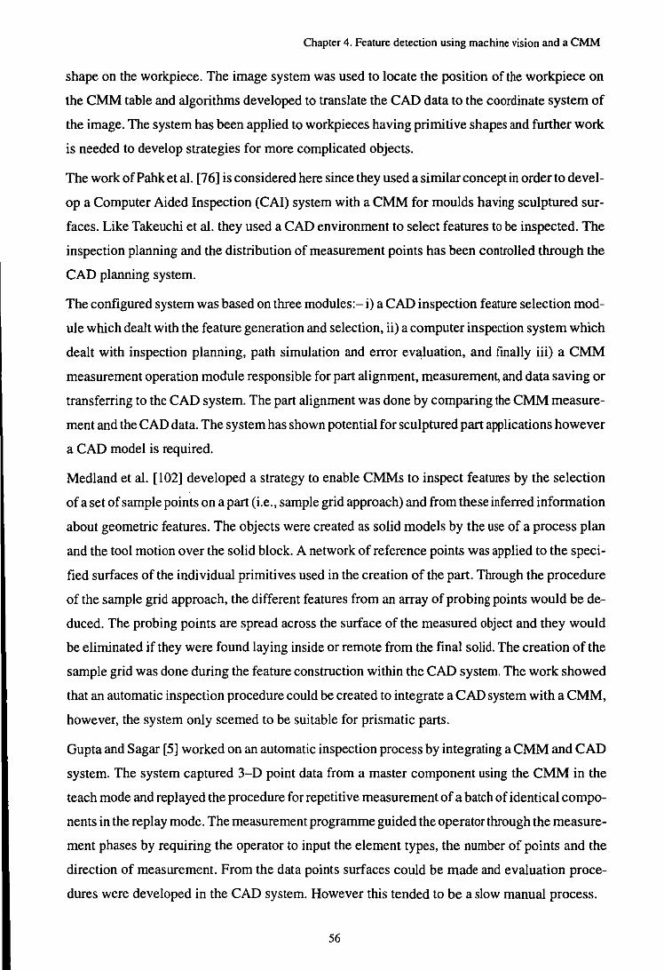
Chapter 4. Feature detection using machine vision and a CMM
shape on the workpiece. The image system was used to locate the position of the workpiece on
the CMM table and algorithms developed to translate the CAD data to the coordinate system of
the image. The system has been applied to workpieces having primitive shapes and further work
is needed to develop strategies for more complicated objects.
The work ofPahket al. [76] is considered here since they used a similar concept in order to devel
op a Computer Aided Inspection (CAI) system with a CMM for moulds having sculptured sur
faces. Like Takeuchi et al. they used a CAD environment to select features to be inspected. The
inspection planning and the distribution of measurement points has been controlled through the
CAD planning system.
The configured system was based on three modules:- i) a CAD inspection feature selection mod
ule which dealt with the feature generation and selection, ii) a computer inspection system which
dealt with inspection planning, path simulation and error evaluation, and finally iii) a CMM
measurement operation module responsible for part alignment, measurement, and data saving or
transferring to the CAD system. The part alignment was done by comparing the CMM measure
ment and the CAD data. The system has shown potential for sculptured part applications however
a CAD model is required.
Medland et al. [102] developed a strategy to enable CMMs to inspect features by the selection
of a set of sample points on a part (i.e., sample grid approach) and from these inferred information
about geometric features. The objects were created as solid models by the use of a process plan
and the tool motion over the solid block. A network of reference points was applied to the speci
fied surfaces of the individual primitives used in the creation of the part. Through the procedure
of the sample grid approach, the different features from an array of probing points would be de
duced. The probing points are spread across the surface of the measured object and they would
be eliminated if they were found laying inside or remote from the final solid. The creation of the
sample grid was done during the feature construction within the CAD system. The work showed
that an automatic inspection procedure could be created to integrate a CAD system with a CMM,
however, the system only seemed to be suitable for prismatic parts.
Gupta and Sagar [5] worked on an automatic inspection process by integrating a CMM and CAD
system. The system captured 3-D point data from a master component using the CMM in the
teach mode and replayed the procedure for repetitive measurement of a batch of identical compo
nents in the replay mode. The measurement programme guided the operator through the measure
ment phases by requiring the operator to input the element types, the number of points and the
direction of measurement. From the data points surfaces could be made and evaluation proce
dures were developed in the CAD system. However this tended to be a slow manual process.
56
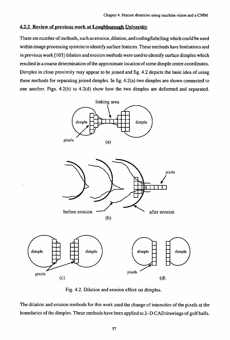
Chapter 4. Feature detection using machine vision and a CMM
4.2.2 Review of previous work at Loughborough University
There are number of methods, such as erosion, dilation, and codingllabelling which could be used
within image processing systems to identify surface features. These methods have limitations and
in previous work [103] dilation and erosion methods were used to identify surface dimples which
resulted in a coarse determination of the approximate location of some dimple centre coordinates.
Dimples in close proximity may appear to be joined and fig. 4.2 depicts the basic idea of using
these methods for separating joined dimples. In fig. 4.2(a) two dimples are shown connected to
one another. Figs. 4.2(b) to 4.2(d) show how the two dimples are deformed and separated.
linking area
\ pixels (a)
pixels
I
before erosion after erosion (b)
'1/ plxe s pixels (c) (d)
Fig. 4.2. Dilation and erosion effect on dimples.
The dilation and erosion methods for this work used the change of intensities of the pixels at the
boundaries of the dimples. These methods have been applied to 2-D CAD drawings of golfballs.
57

Chapter 4. Feature detection using machine vision and a CMM
The method used the difference in intensity level of the dimple boundaries to that of the back
ground and by eroding and dilating the area within these boundaries, the centre of each dimple
was reduced to a dot or small number of pixels.
One of the main problems with this method was not knowing the required number of iterations
for each determination since the dimples were of different sizes and therefore some would reduce
to one pixel sooner than others. The best result obtained was about 35 per cent of the dimples on
a half of the cubic pattern ball. A major weakness of this approach was the inability to detect
dimples around the golf ball equator where the majority of the dimples are concentrated. Dimples
in this area needed fewer erosions to those at the centre of the ball image because the dimples in
the centre are bigger and are more easily identified.
This result was achieved using a good quality 2-D CAD generated drawing, when using a real
ball it is likely that the results would be worse.
4.3 Proposed integration method in this work
The use of 3-D CMMs for the measurement of objects is well established in manufacturing in
dustries and the use of touch probe methods has enabled accurate measurements of prismatic
parts. However, accurate measurement of sculptured surfaces still presents some problems and
there is still no general automated inspection method or system available. Nevertheless, there are
many CAD and CMM integration systems in which the CAD software helps to generate the in
spection routines.
In many instances no CAD model of the objects exist and the "clay" model is in fact the design
specification. In this situation the model needs to be measured in a suitable way such that the in
formation can be input to a CAD system for further processing and development of manufactur
ing information. Programming of a CMM to suit such a system is a lengthy business and the abil
ity to generate programmes automatically is not available. When a component has many features
such as a golf ball the machine vision is an attractive solution to the problem of locating dimple
centre coordinates which then can be transferred to a 3-D CMM for an accurate measurement
of the dimples. Vision methods currently available do not have the required accuracy to measure
the features accurately. However, a vision system could be used to provide an approximation of
the component position which can be used to programme the CMM for probing.
This method is based on the concept of look and touch and consists of a Matrox machine vision
system for the generation of the approximate location of the features and two CMMs, a Ferranti
Merlin and aBrown andSharpeXcel Tesa. TheCMMs were equipped with aRenishawmotorised
probe head arrangement which inspects the features precisely to a high order of accuracy. The
58

Chapter 4. Feature detection using machine vision and a ·CMM
system is integrated to a CAD system to represent the inspected model graphically and to model
the errors within the product. This method should be applicable to many products about which
there is a prior knowledge of the shape.
4.3.1 Method of feature detection
One of the main problems when looking at features using a vision system is determining the ex
tent of features. In prismatic parts distinct edges are present which identify a feature and it is also
possible to construct the feature shape by implication of the feature location, for example inter
section of planes. However, the case of sculptured parts is more difficult due to not knowing the
general shape of the features or the extent. Using a machine vision the information which could
lead to recognition of the features could be interpreted from shadows, from surface discontinu
ities and suitable lighting, however, this is a subjective process. Preliminary tests using a vision
system indicated that the features needed to be enhanced in order to identify them before digitisa
tion. A number of different techniques were used to develop a simple technique for feature detec
tion. In this study the feature marking method used is based on manually placing a small dot inside
of each feature with a marker pen.
4.3.2 Identification of dimples
In order to develop a system to identify the dimple positions on a golf ball with the use of a 2-D
vision system two stages were investigated; I) use of 2-D models i.e., CAD plots and, 2) use of
real golf balls.
In the first stage CAD 2-D drawings of golf balls were used with dimples shown as circles when
they were close to the centre of the drawing, and deforming to ellipses towards the edge, fig. 4.3
is a 2-D CAD model of a golf ball which was produced to the design specification with circular
dimples presented in a cubic pattern. The initial intention in the use of 2-D plots was to test and
develop methods on clear images. Prior to identifying dimple centres the image needed to be pre
pared by removing unwanted portions from the image, e.g., surrounding marks etc.
To detect dimples on a white golf ball it was necessary to enhance the dimples from the back
ground, since only a small number of dimples could be detected due to the lack of contrast be
tween the features and the ball. There were a number of ways which dimples could be presented
for image capturing such as; colouring dimples black or colouring the lands between the dimples,
fig. 4.4 shows the colouring arrangements on golf balls. There were number of problems encoun
tered when golf baIls were used such as, they have shiny surfaces, no sharp edges which could
be used to generate enough contrast for identification, and finally they are the same colour as the
59
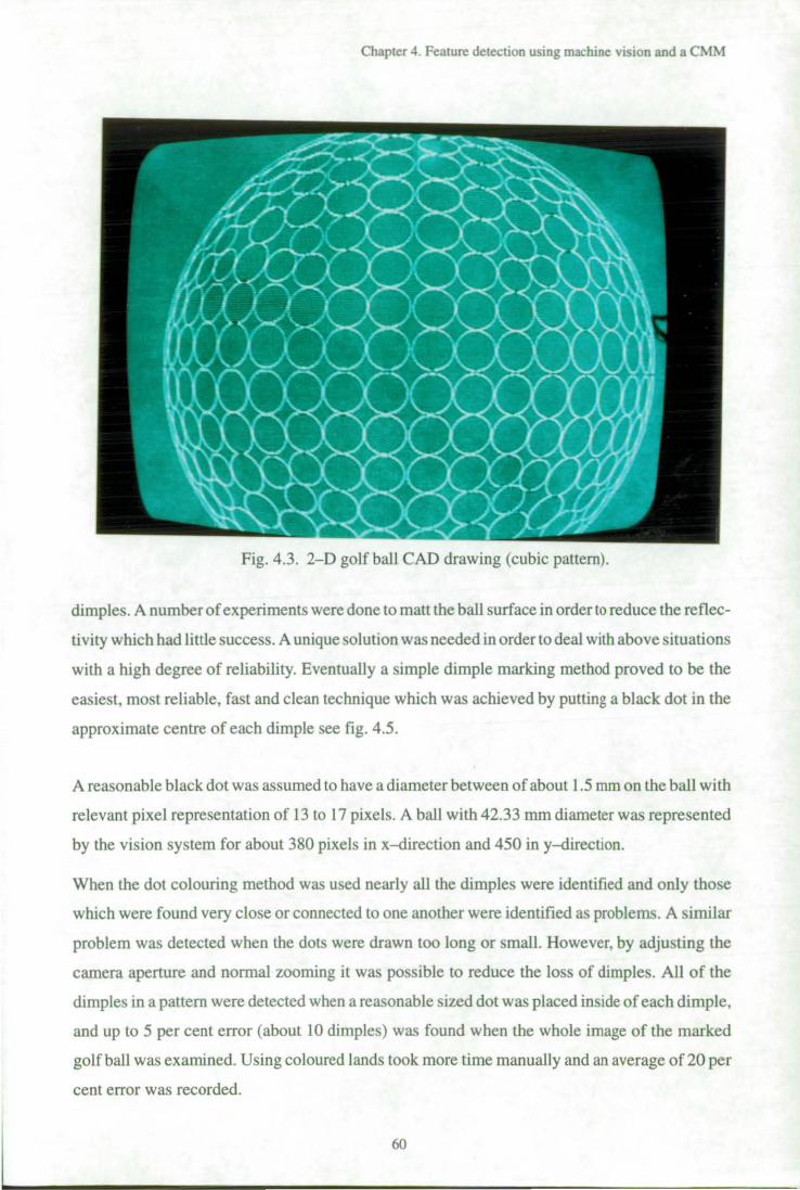
Chapter 4. Feature detection using machine vision and a CMM
Fig. 4.3. 2-D golf ball CAD drawing (cubic pattern).
dimples. A number of experiments were done to matt the ball surface in order to reduce the reflec
tivity which had little success. A unique solution was needed in order to deal with above situations
with a high degree of reliability. Eventually a simple dimple marking method proved to be the
easiest, most reliable, fast and clean technique which was achieved by putting a black dot in the
approximate centre of each dimple see fig. 4.5.
A reasonable black dot was assumed to have a diameter between of about 1.5 mm on the ball with
relevant pixel representation of 13 to 17 pixels. A ball with 42.33 mm diameter was represented
by the vision system for about 380 pixels in x-<lirection and 450 in y-direction.
When the dot colouring method was used nearly all the dimples were identified and only those
which were found very close or connected to one another were identified as problems. A similar
problem was detected when the dots were drawn too long or small. However, by adjusting the
camera aperture and normal zooming it was possible to reduce the loss of dimples. All of the
dimples in a pattern were detected when a reasonable sized dot was placed inside of each dimple,
and up to 5 per cent error (about 10 dimples) was found when the whole image of the marked
golf ball was examined. Using coloured lands took more time manually and an average of20 per
cent error was recorded.
60
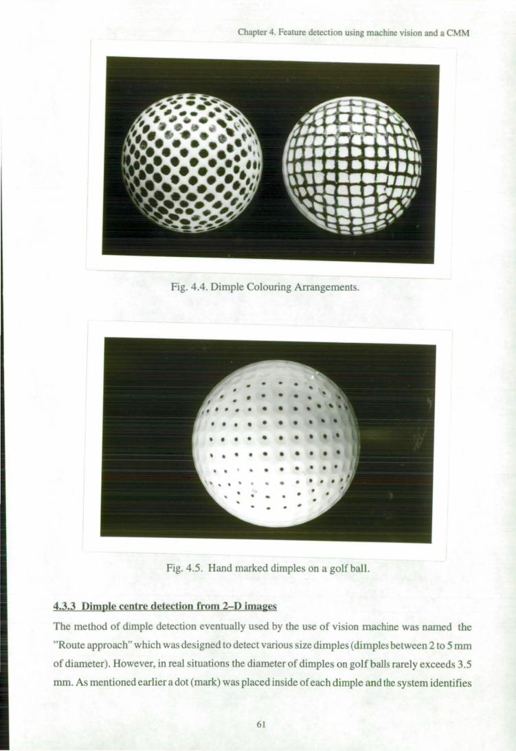
Chapter 4. Feature detection using machine vision and a CMM
Fig. 4.4. Dimple Colouring Arrangements.
• • • , • • • • • • • • , • • •
• • • • • • • • • • • • • • • • • • • • • • • • • • • •
• • • • • • • • • • • • • • • • •
Fig. 4.5. Hand marked dimples on a golf ball.
4.3.3 Dimple centre detection from 2-D ima2es
The method of dimple detection eventually used by the use of vision machine was named the
"Route approach" which was designed to detect various size dimples (dimples between 2 to 5 mm
of diameter). However, in real situations the diameter of dimples on golf balls rarely exceeds 3.5
mm. As mentioned earlier a dot (mark) was placed inside of each dimple and the system identifies
61
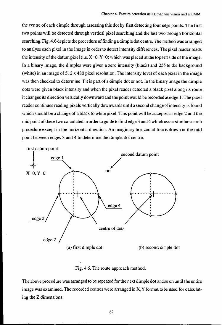
Chapter 4. Feature detection using machine vision and a CMM
the centre of each dimple through assessing this dot by first detecting four edge points. The first
two points will be detected through vertical pixel searching and the last two through horizontal
searching. Fig. 4.6 depicts the procedure of finding a dimple dot centre. The method was arranged
to analyse each pixel in the image in order to detect intensity differences. The pixel reader reads
the intensity of the datum pixel (i.e. X=O, Y =0) which was placed at the top left side of the image.
In a binary image, the dimples were given a zero intensity (black) and 255 to the background
(white) in an image of 512 x 480 pixel resolution. The intensity level of each pixel in the image
was then checked to determine if it is part of a dimple dot or not. In the binary image the dimple
dots were given black intensity and when the pixel reader detected a black pixel along its route
it changes its direction vertically downward and the point would be recorded as edge I. The pixel
reader continues reading pixels vertically downwards until a second change of intensity is found
which should be a change of a black to white pixel. This point will be accepted as edge 2 and the
mid point of these two calculated in order to guide to find edge 3 and 4 which uses a similar search
procedure except in the horizontal direction. An imaginary horizontal line is drawn at the mid
point between edges 3 and 4 to determine the dimple dot centre.
first datum point
~~ second datum point
/ X=o, y=o
edge 4
edge 3
centre of dots
edge 2
(a) first dimple dot (b) second dimple dot
Fig. 4.6. The route approach method.
The above procedure was arranged to be repeated for the next dimple dot and so on until the entire
image was examined. The recorded centres were arranged in X,Y format to be used for calculat
ing the Z dimensions.
62
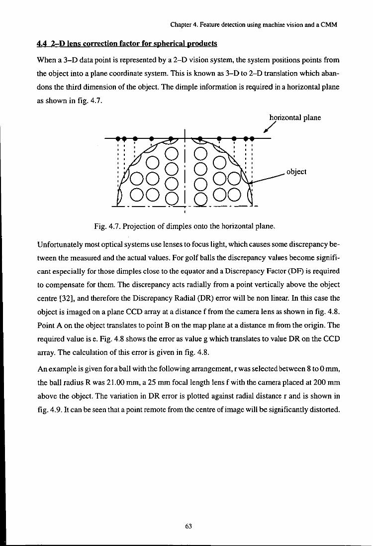
Chapter 4. Feature detection using machine vision and a CMM
4.4 k=D lens correction factor for spherical products
When a 3-D data point is represented by a 2-D vision system, the system positions points from
the object into a plane coordinate system. This is known as 3-D to 2-D translation which aban
dons the third dimension of the object. The dimple information is required in a horizontal plane
as shown in fig. 4.7.
horizontal plane
/
object
Fig. 4.7. Projection of dimples onto the horizontal plane.
Unfortunately most optical systems use lenses to focus light, which causes some discrepancy be
tween the measured and the actual values. For golf balls the discrepancy values become signifi
cant especially for those dimples close to the equator and a Discrepancy Factor (DF) is required
to compensate for them. The discrepancy acts radially from a point vertically above the object
centre [32], and therefore the Discrepancy Radial (DR) error will be non linear. In this case the
object is imaged on a plane CCD array at a distance f from the camera lens as shown in fig. 4.8.
Point A on the object translates to point B on the map plane at a distance m from the origin. The
required value is e. Fig. 4.8 shows the error as value g which translates to value DR on the CCD
array. The calculation of this error is given in fig. 4.8.
An example is given for a ball with the following arrangement, r was selected between 8 to 0 mm,
the ball radius R was 21.00 mm, a 25 mm focal length lens f with the camera placed at 200 mm
above the object. The variation in DR error is plotted against radial distance r and is shown in
fig. 4.9. It can be seen that a point remote from the centre of image will be significantly distorted.
63
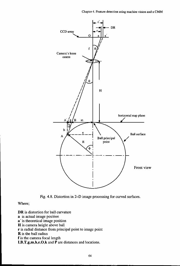
Chapter 4. Feature detection using machine vision and a CMM
CCD array
Camera's lense centre
" l /
/ /
/ /
/ /
/ /
/ /
DR
a
f
H
/ A' /
horizontal map plane
---=---j\ , Ball principal
R point
<1>,
------1------,
1 ,
1
Front view
Fig. 4.8. Distortion in 2-D image processing for curved surfaces.
Where;
DR is distortion for ball curvature a is actual image position a' is theoretical image position H is camera height above ball r is radial distance from principal point to image point R is the ball radius f is the camera focal length I,B,T,g,m,h,e,O,k and P are distances and locations.
64
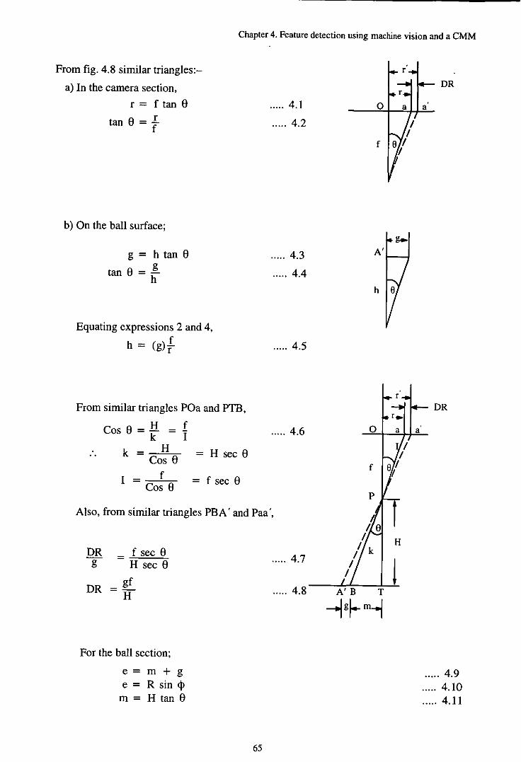
Chapter 4. Feature detection using machine vision and a CMM
From fig. 4.8 similar triangles:
a) In the camera section,
r= ftan8
tan8=!
b) On the baIl surface;
g=htan8
tan8=..[ h
Equating expressions 2 and 4,
h = (g){
From similar triangles POa and PTB,
Cos8=H =! k I
k= H =Hsec8 Cos 8
1= f =fsec8 Cos 8
..... 4.1
..... 4.2
..... 4.3
..... 4.4
..... 4.5
..... 4.6
Also, from similar triangles PBA' and Paa',
DR g
f sec 8 = ~H;-=se=-c--'8;;-
gf DR =jf
For the baIl section;
e = m + g e=Rsin<j> m=Htan8
..... 4.7
..... 4.8
65
f
DR
DR
..... 4.9 ..... 4.10 ..... 4.11
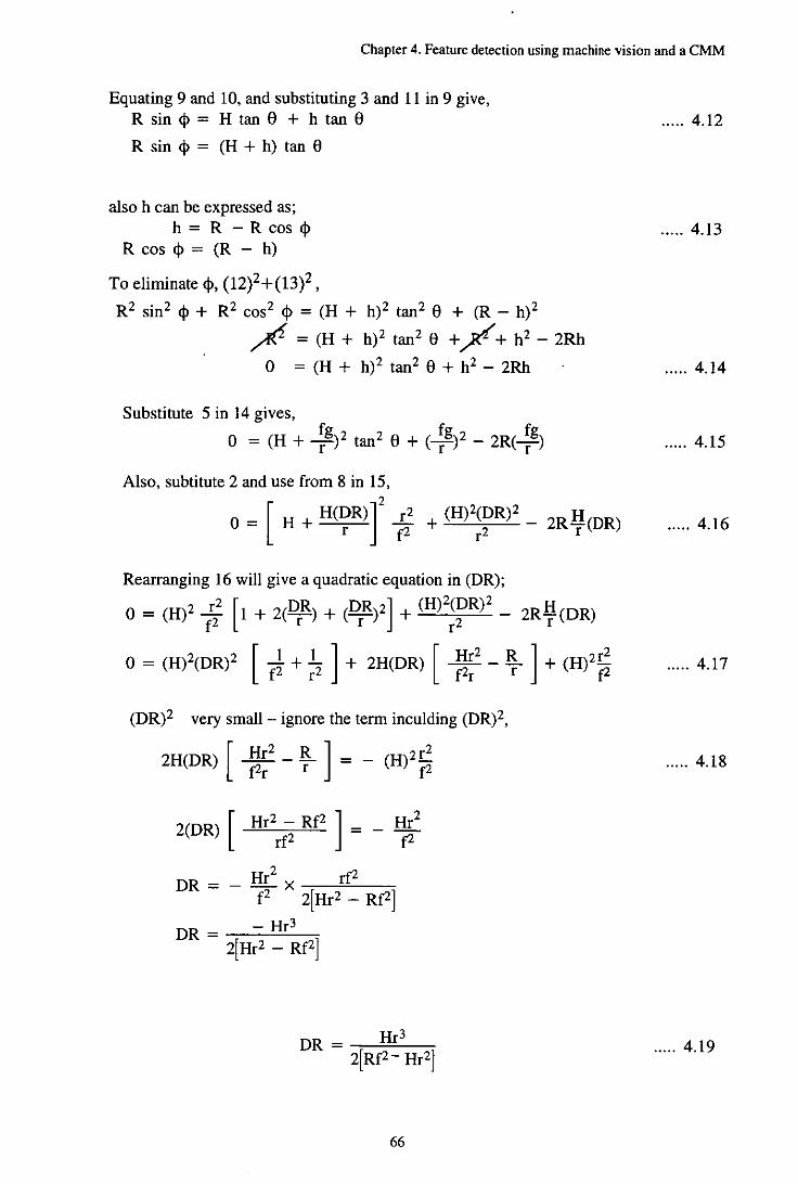
Chapter 4. Feature detection using machine vision and a CMM
Equating 9 and 10, and substituting 3 and 11 in 9 give, Rsin<j>= HtanS + htanS
R sin <j> = (H + h) tan S
also h can be expressed as; h=R-Rcos<j>
R cos <j> = (R - h)
To eliminate <j>, (12)2+(13)2,
R2 sin2 <j> + R2 cos2 <j> = (H + h)2 tan2 S + (R - h)2
~ = (H + h)2 tan2 e + / + h2 - 2Rh
o = (H + h)2 tan2 e + h2 - 2Rh
Substitute 5 in 14 gives,
o = (H + ;g)2 tan2 e + ( ;g)2 - 2R( ;g)
Also, subtitute 2 and use from 8 in 15, 2
o = [ H + H(DR)] ...r!. r f2
Rearranging 16 will give a quadratic equation in (DR);
o = (H)2...r!. [1 + 2(DR) + (DR)2] + (H)2(DR)2 - 2R Hr (DR) f2 r r r2
o = (H)2(DR)2 [-.l + 1.. ] + 2H(DR) [ Hr2 _ B.. ] + (H)2f2 f2 r2 f2r r f2
(DR)2 very small- ignore the term inculding (DR)2,
2H(DR) [ Hr2 _ B.. ] = _ (H)2f2 f2r r f2
2(DR) [ Hr2 - Rf2 ] = _ Hr2 rf2 f2
DR = - Hr2 x rf2 f2 2[Hr2 - Rf2]
DR = - Hr3
2[Hr2 - Rf2]
66
..... 4.12
..... 4.13
..... 4.14
..... 4.15
..... 4.16
..... 4.17
..... 4.18
..... 4.19
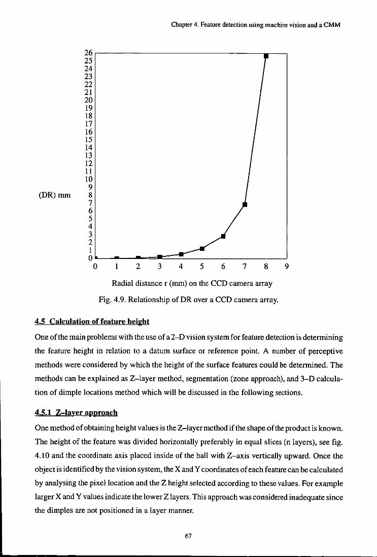
(OR) mm
Chapter 4. Feature detection using machine vision and a CMM
26r---------------------------__ ,--~ 25 24 23 22 21 20 19 18 17 16 15 14 13 12 11 10 9 8 7 6 5 4 3 2
6~~~~==~~-~--------------~ o I 2 3 4 5 6 7 8
Radial distance r (mm) on the CCD camera array
Fig. 4.9. Relationship of OR over a CCO camera array.
9
4.5 Calculation of feature height
One of the main problems with the use of a 2-0 vision system for feature detection is determining
the feature height in relation to a datum surface or reference point. A number of perceptive
methods were considered by which the height of the surface features could be determined. The
methods can be explained as Z-Iayer method, segmentation (zone approach), and 3-0 calcula
tion of dimple locations method which will be discussed in the following sections.
4.5.1 Z-Iayer approach
One method of obtaining height values is the Z-Iayer method if the shape of the product is known.
The height of the feature was divided horizontally preferably in equal slices (n layers), see fig.
4.10 and the coordinate axis placed inside of the ball with Z-axis vertically upward. Once the
object is identified by the vision system, the X and Y coordinates of each feature can be calculated
by analysing the pixellocation and the Z height selected according to these values. For example
larger X and Y values indicate the lower Z layers. This approach was considered inadequate since
the dimples are not positioned in a layer manner.
67
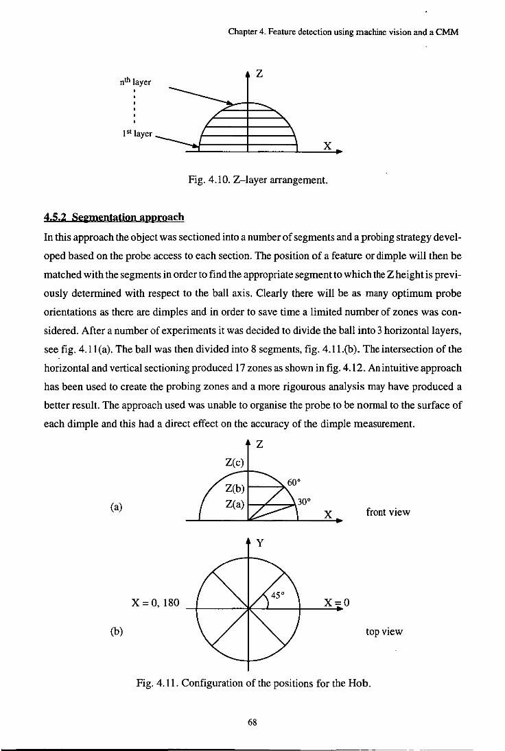
Chapter 4. Feature detection using machine vision and a CMM
nth layer z
o
I st layer
x
Fig. 4.10. Z-Iayer arrangement.
4.5.2 Segmentation approach
In this approach the object was sectioned into a number of segments and a probing strategy devel
oped based on the probe access to each section. The position of a feature or dimple will then be
matched with the segments in order to find the appropriate segment to which the Z height is previ
ously determined with respect to the ball axis. Clearly there will be as many optimum probe
orientations as there are dimples and in order to save time a limited number of zones was con
sidered. After a number of experiments it was decided to divide the ball into 3 horizontal layers,
see fig. 4.11 (a). The ball was then divided into 8 segments, fig. 4.11.(b). The intersection of the
horizontal and vertical sectioning produced 17 zones as shown in fig. 4.12. An intuitive approach
has been used to create the probing zones and a more rigourous analysis may have produced a
better result. The approach used was unable to organise the probe to be normal to the surface of
each dimple and this had a direct effect on the accuracy of the dimple measurement.
Z
Z(c)
(a) x front view
y
X=0,180 X=O
(b) top view
Fig. 4.11. Configuration of the positions for the Hob.
68
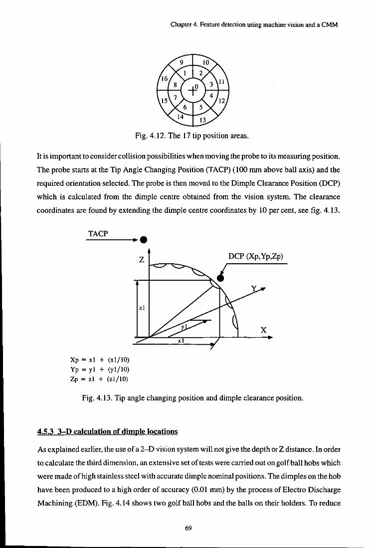
Chapter 4. Feature detection using machine vision and a CMM
Fig. 4.12. The 17 tip position areas.
It is important to consider collision possibilities when moving the probe to its measuring position.
The probe starts at the Tip Angle Changing Position (TACP) (lOO mm above ball axis) and the
required orientation selected. The probe is then moved to the Dimple Clearance Position (DCP)
which is calculated from the dimple centre obtained from the vision system. The clearance
coordinates are found by extending the dimple centre coordinates by 10 per cent, see fig. 4.13.
TACP ----....
Xp = xl + (xl/IO)
Yp = yl + (yl/IO)
zp = zl + (zl/IO)
zl
DCP (Xp,Yp,Zp)
Fig. 4.13. Tip angle changing position and dimple clearance position.
4.5.3 3-D calculation of dimple locations
As explained earlier, the use of a 2-D vision system will not give the depth or Z distance. In order
to calculate the third dimension, an extensive set of tests were carried out on golf ball hobs which
were made of high stainless steel with accurate dimple nominal positions. The dimples on the hob
have been produced to a high order of accuracy (0.01 mm) by the process ofElectro Discharge
Machining (EDM). Fig. 4.14 shows two golf ball hobs and the balls on their holders. To reduce
69
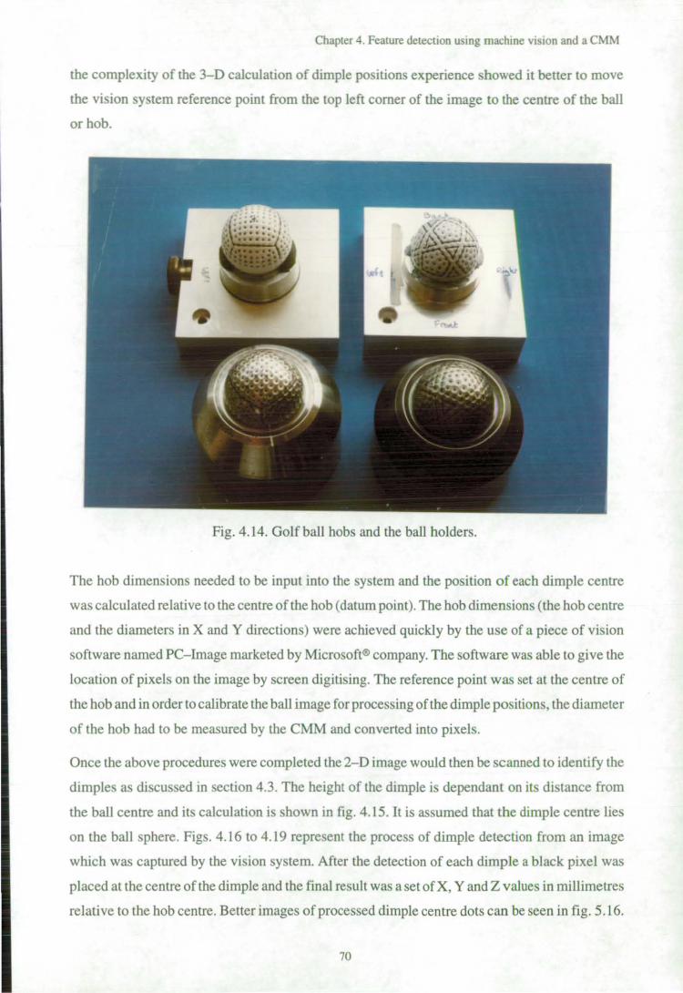
Chapter 4. Feature detection using machine vision and a CMM
the complexity of the 3-D calculation of dimple positions experience bowed it better to move
the vision system reference point from the top left corner of the image to the centre of the ball
or hob.
Fig. 4.14. Golf ball hobs and the ball holders.
The hob dimensions needed to be input into the system and the position of each dimple centre
was calculated relative to the centre of the hob (datum point). The hob dimensions (the hob centre
and the diameters in X and Y directions) were achieved quickly by the use of a piece of vision
software named PC-Image marketed by Microsoftl!> company. The software was able to give the
location of pixels on the image by screen digitising. The reference point was set at the centre of
the hob and in order to calibrate the ball image for processing of the dimple positions, the diameter
of the hob had to be measured by the CMM and converted into pixels.
Once the above procedures were completed the 2-D image would then be scanned to identify the
dimples as discussed in section 4.3. The height of the dimple is dependant on its distance from
the ball centre and its calculation is shown in fig. 4.15. It is assumed that the dimple centre lies
on the ball sphere. Figs. 4.16 to 4.19 represent the process of dimple detection from an image
which was captured by the vision system. After the detection of each dimple a black pixel was
placed at the centre of the dimple and the final result was a setofX, Y and Z values in millimetres
relative to the hob centre. Better images of processed dimple centre dots can be seen in fig. 5.16.
70
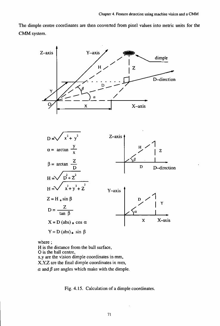
Chapter 4. Feature detection using machine vision and a CMM
The dimple centre coordinates are then converted from pixel values into metric units for the
CMMsystem.
Z-axis
//i~ :/ I Z
/ --r--;t<""""':;,;'-- - - - - - - -
y a= arctan -
x
x X-axis
Z-axis
Z ~= arctan -
D D D-direction
H=VrJ+l / 2 2 2
H=V x+y +Z
Z=H*sin~
D= Z tan ~
X = D (abs) * cos a
Y = D (abs) * sin ~
where;
Y-axis
H is the distance from the ball surface, o is the ball centre, x,y are the vision dimple coordinates in mm, X, Y,Z are the final dimple coordinates in mm, a and f3 are angles which make with the dimple.
x
Fig. 4.15. Calculation of a dimple coordinates.
71
X-axis

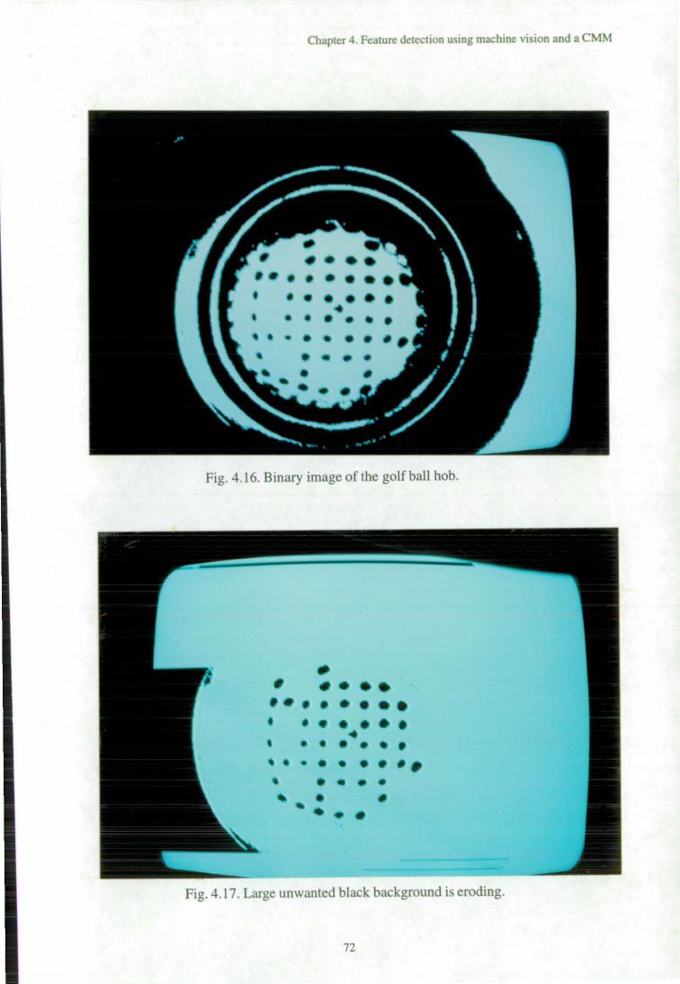
Chapter 4. Feature detection using machine vision and a CMM
• • • • • • • • • • • • • • • • • • • • • • • • • • •
• • • •
Fig. 4.16. Binary image of the golf ball hob.
• • • • •• •• • • • • • • • • • • • • • • • • • • • • • • • • • • • • -. • • • • •
• • .. • • •
Fig. 4.17. Large unwanted black background is eroding.
72

o
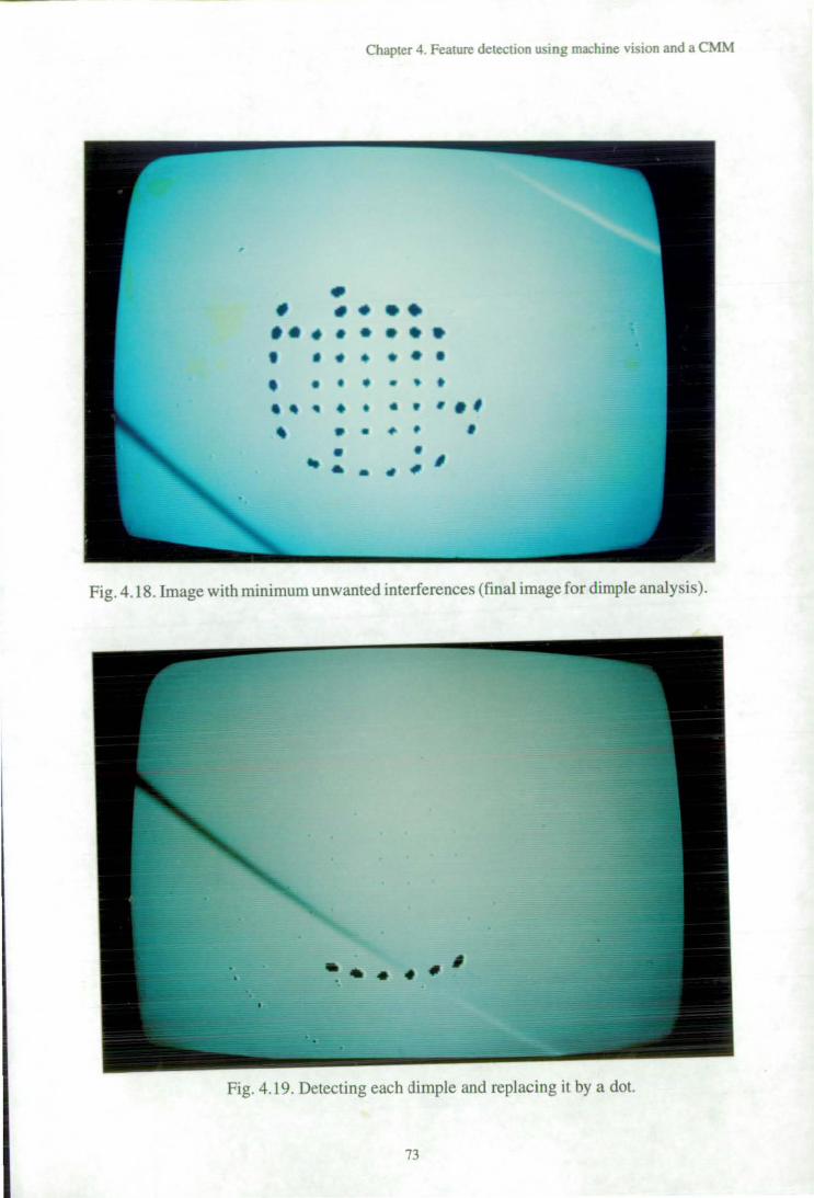
Chapter 4. Feature detection using machine vision and a CMM
• • • •• • • • • • • • • • • • • • • • • • •
4 .. • • • • · ., • • • • • • • .. .. 4'
, • -
Fig. 4.IS.lmage with minimum unwanted interferences (fmal image for dimple analysis).
Fig. 4.19. Detecting each dimple and replacing it by a dot.
73
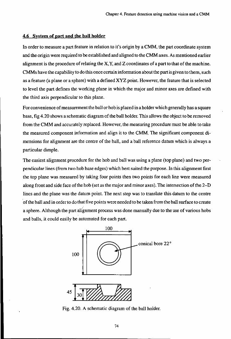
Chapter 4. Feature detection using machine vision and a CMM
4.6 System of part and the ball holder
In order to measure a part feature in relation to it's origin by a CMM, the part coordinate system
and the origin were required to be established and aligned to the CMM axes. As mentioned earlier
alignment is the procedure of relating the X, Y, and Z coordinates of a part to that of the machine.
CMMs have the capability to do this once certain information about the part is given to them, such
as a feature (a plane or a sphere) with a defined XYZ point. However, the feature that is selected
to level the part defines the working plane in which the major and minor axes are defined with
the third axis perpendicular to this plane.
For convenience of measurement the ball or hob is placed in a holder which generally has a square
base, fig 4.20 shows a schematic diagram of the ball holder. This allows the object to be removed
from the CMM and accurately replaced. However, the measuring procedure must be able to take
the measured component information and align it to the CMM. The significant component di
mensions for alignment are the centre of the ball, and a ball reference datum which is always a
particular dimple.
The easiest alignment procedure for the hob and ball was using a plane (top plane) and two per
pendicular lines (from two hob base edges) which best suited the purpose. In this alignment first
the top plane was measured by taking four points then two points for each line were measured
along front and side face ofthe hob (set as the major and minor axes). The intersection of the 2-D
lines and the plane was the datum point. The next step was to translate this datum to the centre
'ofthe ball and in order to do that five points were needed to be taken from the ball surface to create
a sphere. Although the part alignment process was done manually due to the use of various hobs
and balls, it could easily be automated for each part.
100
conical bore 22 0
100
Fig. 4.20. A schematic diagram of the ball holder.
74

Chapter 4. Feature detection using machine vision and a CMM
4.7 Probing strategy
Once the position of feature data points were known it was required to develop a strategy to guide
the probe to inspect and assess the features. The probe needed to approach the feature normal to
the work surface and avoid collision with the ball when moving from one side to the other. The
most practical way was to guide the probe along a 3-D vector between the ball centre and each
vision data point.
A dimple sphere was generated by taking five readings from each dimple enabling a second more
accurate 3-D vector to be created between the dimple sphere centre and the baIl. The feature was
then measured once more using nineteen readings and a more accurate dimple sphere created.
As mentioned before there are recommendations for the minimum number of points required to
fit a geometric feature. Nineteen readings was found to be adequate, and readings beyond this
did not increase the accuracy of the measurement significantly.
In order to achieve accurate measurements for each dimple, the CMM software required informa
tion about each tip and probe configuration (orientation, height, clearance etc.). As explained in
chapter 3 each probe and probe orientation needs to be qualified or calibrated against a reference
sphere. This process normally requires touching the reference sphere at 3 levels, 5 times in remote
positions. In this case 25 readings were taken. This information was held in a qualification file.
In order to keep the measurement accuracy as high as possible it is important that the qualification
file should be executed every time the probe configuration is changed, and also executed period
ically for system confirmation. The majority of CMMs have an automatic tip qualification soft
ware and there are usually two types of calculation for an effective probe diameter (the best poss
ible tip diameter). The first is the computation of a single effective probe diameter for each probe
being qualified and the other is based on the approach direction of the measurement point. In this
case the latter method was used in which the CMM automatically computed the effective probe
diameter from the touched points which improved the accuracy of the measurement.
4.7.1 Restrictions on different CMMs
Apart from the recommended procedures for use of a TIP there is a design restriction with the
PH9 that the probe can only increment in steps of 7.5· in both horizontal and vertical planes. In
addition to this some CMM software is only capable of saving a certain number of orientations,
for example the Ferranti CMM could save up to 20 orientations in a calibration file while the Tesa
CMM allows up to 700 orientations.
To measure each dimple it was required to use different probe orientations since dimples were
spread all over the ball. In order to do this, two angles the yaw A and pitch B were needed to be
75
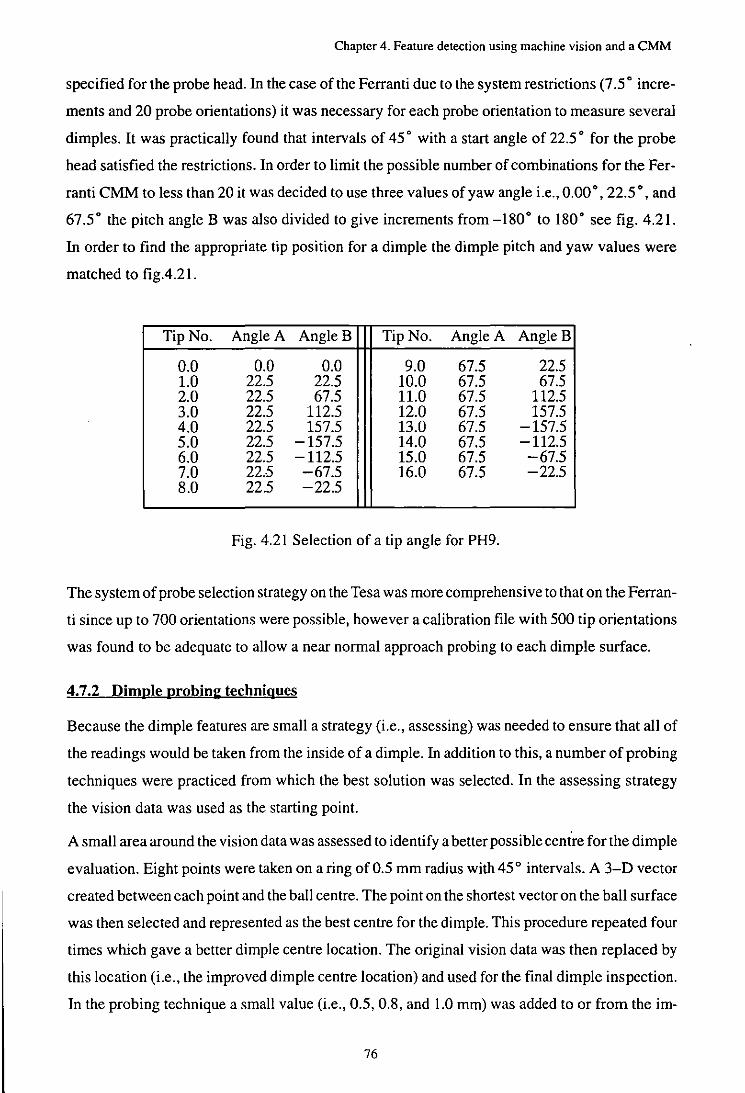
Chapter 4. Feature detection using machine vision and a CMM
specified for the probe head. In the case of the Ferranti due to the system restrictions (7.5· incre
ments and 20 probe orientations) it was necessary for each probe orientation to measure several
dimples. It was practically found that intervals of 45· with a start angle of 22.5· for the probe
head satisfied the restrictions. In order to limit the possible number of combinations for the Fer
ranti CMM to less than 20 it was decided to use three values ofyaw angle i.e., 0.00·,22.5·, and
67.5· the pitch angle B was also divided to give increments from -180· to 180· see fig. 4.21.
In order to find the appropriate tip position for a dimple the dimple pitch and yaw values were
matched to fig.4.21.
Tip No. Angle A AngleB Tip No. Angle A Angle B
0.0 0.0 0.0 9.0 67.5 22.5 1.0 22.5 22.5 10.0 67.5 67.5 2.0 22.5 67.5 11.0 67.5 112.5 3.0 22.5 112.5 12.0 67.5 157.5 4.0 22.5 157.5 13.0 67.5 -157.5 5.0 22.5 -157.5 14.0 67.5 -112.5 6.0 22.5 -112.5 15.0 67.5 -67.5 7.0 22.5 -67.5 16.0 67.5 -22.5 8.0 22.5 -22.5
Fig. 4.21 Selection of a tip angle for PH9.
The system of probe selection strategy on the Tesa was more comprehensive to that on the Ferran
ti since up to 700 orientations were possible, however a calibration file with 500 tip orientations
was found to be adequate to allow a near normal approach probing to each dimple surface.
4.7.2 Dimple probing techniques
Because the dimple features are small a strategy (i.e., assessing) was needed to ensure that all of
the readings would be taken from the inside of a dimple. In addition to this, a number of probing
techniques were practiced from which the best solution was selected. In the assessing strategy
the vision data was used as the starting point.
A small area around the vision data was assessed to identify a better possible centre for the dimple
evaluation. Eight points were taken on a ring of 0.5 mm radius with 45 0 intervals. A 3-D vector
created between each point and the ball centre. The point on the shortest vector on the ball surface
was then selected and represented as the best centre for the dimple. This procedure repeated four
times which gave a better dimple centre location. The original vision data was then replaced by
this location (i.e., the improved dimple centre location) and used for the final dimple inspection.
In the probing technique a small value (i.e., 0.5, 0.8, and 1.0 mm) was added to or from the im-
76
Chapter 4. Feature detection using machine vision and a CMM
proved vision coordinate values to which the probe moved to take readings from the dimple. This
procedure was repeated three times with five readings for the fust time and nineteen for the sec
ond and third times to assure the accuracy of the measurement. Each set of readings was fitted
into a sphere using a routine named Dimple Sphere (OS) and from the last set of readings the OS
was constructed from which the dimple characteristics were calculated.
One of the main difficulties with the above methods was the way of incrementing probing points
in order to take equally spaced readings from inside of each dimple. Since the CMM selects a 2-D
working plane depending on the position of the dimple it was difficult to control the probe incre
mentation since the working plane constantly changed. It also should be remembered that it is
not normal practice for a CMM to measure a very small portion of a feature and fit a feature into
it since small errors can be significantly amplified.
The solution used was to develop a measuring approach by taking a vector from the ball centre
through the detected dimple centre. Five points 1 mm apart were selected around the vector.
These probed points gave a first approximation for the dimple sphere. However, this approxima
tion gave a better indication of the dimple centre and chord diameter which allowed a more accu-
. rate approach vector to be calculated and the measuring points moved further apart. To enable
accurate measurement to take place nineteen readings were taken for each dimple, one at the
centre and six at three levels around the dimple centre point. To ensure the accuracy, repeatability
and reliability of the measurement another set of nineteen readings were taken for each dimple
in the same manner as before. The same measuring approach was taken for each dimple which
took into account the required clearance position. The method was automated with a developed
CMM programme named BALLINSP.
A set of equations were developed in order to calculate the required dimple characteristics e.g.,
dimple depth and chord diameter. Fig. 4.22 shows calculations to find the required information
about each dimple. Fig. 4.23 is a flow diagram of the automated inspection procedure for dimples
on golf balls.
77
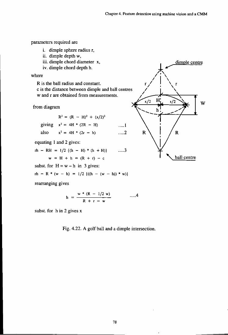
Chapter 4. Feature detection using machine vision and a CMM
parameters required are
where
i. dimple sphere radius r, ii. dimple depth w, iii. dimple chord diameter x, iv. dimple chord depth h.
R is the ball radius and constant. c is the distance between dimple and ball centres w and r are obtained from measurements.
from diagram
R' = (R - H)' + (x/2)'
giving x2 = 4H • (2R - H)
also x2 = 4H • (2r - h)
equating I and 2 gives:
rh - RH = 1/2 {(h - H) • (h + H)}
w = H + h = (R + r) - c
subst. for H = w - h in 3 gives:
..... 1
..... 2
.... .3
rh - R • (w - h) = 1/2 {«h - (w - h)) • w)}
rearranging gives
I.
h = w· (R - 1/2 w) .... .4 R + r - w
subst. for h in 2 gives x
I dimple centre ± ......... /,'
/1\ ri' r I , I ,
/ _--:r-=:::::-:...-----r w
'\ ball centre
Fig. 4.22. A golf ball and a dimple intersection.
78
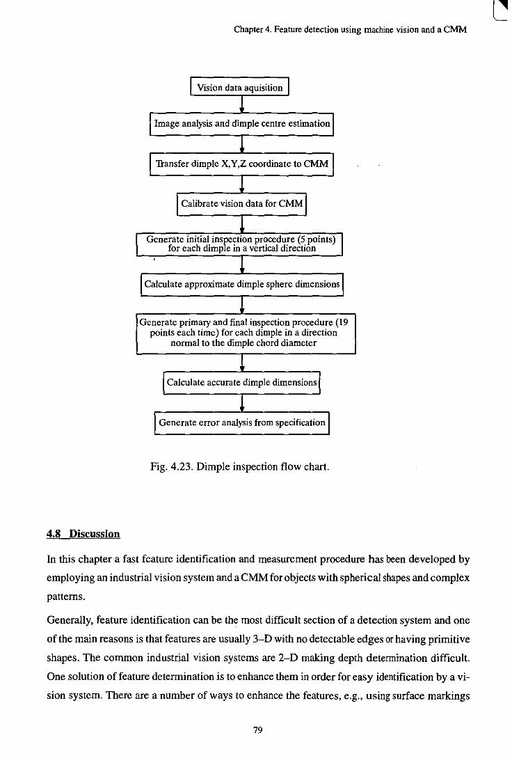
4.8 Discussion
Chapter 4. Feature detection using machine vision and a CMM
I Vision data aquisition I !
I Image analysis and dimple centre estimation I !
I Transfer dimple X, Y,Z coordinate to CMM I !
I Calibrate vision data for CMM I i
Generate initial inspection procedure (5 points) I for each dimple in a vertical direction
l Calculate approximate dimple sphere dimensionsJ
! Generate primary and final inspection procedure (19
points each time) for each dimple in a direction normal to the dimple chord diameter
I Calculate accurate dimple dimensions I ! l Generate error analysis from specificationJ
Fig. 4.23. Dimple inspection flow chart.
In this chapter a fast feature identification and measurement procedure has been developed by
employing an industrial vision system and a CMM for objects with spherical shapes and complex
patterns.
Generally, feature identification can be the most difficult section of a detection system and one
of the main reasons is that features are usually 3-D with no detectable edges or having primitive
shapes. The common industrial vision systems are 2-D making depth determination difficult.
One solution of feature determination is to enhance them in order for easy identification by a vi
sion system. There are a number of ways to enhance the features, e.g., using surface markings
79

Chapter 4. Feature detection using machine vision and a CMM
such as dots, grids, patterns and stripes, or use special light arrangement methods to generate a
similar effect on the object surface. The developed method in this work was based on enhancing
the features by marking and the most successful was simply to place a dot at the centre. The prob-, ing strategy for the CMM was developed based on knowing a point on each feature. With a prior
knowledge of the feature shape it was then possible to detect and locate the dots by a set of devel
oped algorithms and softwares which allowed the evaluation of the features to the machine
highest accuracy. This method proved to be very simple and effective and may possibly be used
elsewhere with some modifications to the system in order to be applicable to other forms of sculp
tured surfaces such as turbine blades, shoe lasts etc.
80
Chapter 5. Multi-Image superimposition technique ... surfaces
CHAPTER 5
MULTI-IMAGE SUPERIMPOSITION TECHNIQUE (MIST) FOR PATTERN FEATURES ON SPHERICAL SURFACES
5.0 Introduction
The feature identification process previously described can determine the approximate location
of features on the object. Once these locations have been determined a measuring method can
be employed to determine the actual position and characteristics of the features in relation to the
main body. However, in the case of complex products with curved surfaces it is difficult to ident
ify features close to and below the parting line or equator when they are viewed from one position
above the object. One solution to this type of problem is to view the object a number of times from
different directions and combine the information. The concept has been applied by other re
searchers [2,23,34,95] to measure approximate part shape, however, the integration of the
method with a CMM for accurate identification and measurement of spherical or curved features
has received little attention.
The generated technique for this work is named Multi-Image Superimposing Technique (MIST)
which enables the inspection system to capture all features on the object of interest, and then
calculate relevant feature data for an accurate inspection. The technique captures desired features
within a detectable zone (an area of confidence for each captured image in order to prevent poss
ible noise intrusion). Each feature location is defined by X,Y, and Z coordinates of its centre i.e.,
a feature datum coordinate. The coordinates describing the feature are related to the vision
coordinate system and must be transformed to a common axis (i.e., world coordinate system) for
consistency of the inspection results.
The objective of any feature identification system using machine vision is to obtain complete ob
ject and . feature identification with the minimum number of viewing positions. Obviously the
minimum possible viewing arrangements would be two (i.e., back and front) but this would not
necessarily identify all aspects of the object. As more viewing positions are included then its obvi
ous that parts of the object will be viewed a number of times. Early work [9] showed that for the
golf ball situation in areas near the edge of the ball it was difficult to identify dimple features dis
tinctly. It was decided to use 5 camera positions because of, ease of image manipulation, and to
establish a method which was certain to lead to a satisfactory solution which could then be the
basis for future improvement. However, this meant that there could be up to 3 overlapping areas,
81
Chapter 5. Multi-Image superimposition technique ... surfaces
shown as areas A in fig. 5.7. It was important to be certain that dimple information was not repli
cated as this would mean repeat probing of some dimples. A technique was required where it was
possible to censor repeated features.
The area of certainty or confidence can be approximated to a circular ring and by knowing the
size of the overlapped areas it was possible to detennine the number of features covered by them.
A number of mathematical methods and approaches were developed to model these areas. Fea
tures outside of the detecting ring would not be recorded but the ring dimensions need to be opti
mised in order to reduce the number of repeated features. The result of this modelling was the
detennination of complete coverage of the ball for the minimum processing time by trimming
off the replicated data in order to achieve one set of data points.
5.1 Feature identification by multi-images
Although, researchers in the area of 3-D recognition use a vision system of some sort for their
applications, they apply a variety of methods to recognise or identify parts. On prismatic parts
where there are interfaces of surfaces or edges, these can be used to more easily locate the position
of features, however, for curved surfaces without obvious edges, different solutions are needed.
In theory to detect features on a golf ball it should be possible to position a camera above the ball
or hob and see all of the dimples on half of the object. Clearly those dimples at the centre of the
ball will look circular, with the shape becoming more elliptical as the dimple moves towards the
perimeter, fig. 4.3, visually it is still possible to identify centres but with increased difficulty. It
was apparent that a more suitable technique was needed in order to capture all dimples.
Stereo vision has been used mainly to identify positions and shapes of3-0 objects. In this method
two or more cameras are used to image a point on the surface of an object in different relative
positions. By analysing the corresponding point in different images, the location of the required
3-D point can be calculated. The significant difficulty of a stereo system however, is to determine
which point in one image corresponds to a given point in the other image. Furthermore, the two
optical axes of the cameras should be aligned precisely to match the two images. Clenk and Ba
chank [95] used this method to extract 3-D information and to reconstruct the object surface in
a robot works pace. The object of interest was viewed by n pairs of cameras. Cho et al [36] used
a similar method by using one camera which was fixed to a CMM ram and arranged to capture
two images along the X-axis of the machine. The object on the table of the CMM would have
projected onto it a grid of spots in order to speed up the process of the point matching. The system
would need further sophistication if the CMM was not used since small alignment errors would
cause inaccurate results due to the incomplete stereo matching.
82
Chapter 5. Multi-Image superimposition technique ... surfaces
Other researchers [23,25,34,97] used multiple 2-D images to extract features for visual inspec
tion and recognition. The main advantage of using this method over other 3-D surface analyses
methods e.g. a stereo vision, is speed, ease of use and it is less complex to extract information
from objects.
5.2 Proposed one camera multi-image superimposed method
In essence, an image superimposing technique is a method which maps (overlaps) images of the
same scene on top of each other taken from different positions. If good analysis methods are avail
able this allows more precise information of areas which are difficult to evaluate.
The MIST is arranged to determine and inspect three Dimensional Sculptured Surfaces (3-DSS),
which have shapes, geometrical features or are of a free form nature. In image analysis it is
necessary to determine a method to reference a feature, this reference value can be used to locate
the feature from a global datum. For the objects in this case the reference point was the dimple
centre and the datum was the bailor hob centre.
The proposed MIST employs the same vision arrangement as that used for the one camera method
(chapter 4). In this technique feature information will be extracted from different images and re
ferred to an individual reference point (i.e., datum) in each image. The datums selected were al
ways the ball centre, errors in datum position of up to 1.0 mm have shown little effect on the
dimple position values.
The MIST uses a number of different views from an object and the feature data.for each view
was arranged to be calculated in 3-D. The images are individually processed and the information
related to each image stored in the same data file. The simplest case of using the technique was
to utilise a minimum of two images from the object taken from different positions. This often
would limit the application of the system since objects with hidden features would not be exposed
by the camera regardless of the camera position. In order to establish the technique, the easiest
case was chosen and that was to use five images from the object. The five images from the object
were arranged to be taken with one image from the top of the object and four images from the
sides of the object. The camera was positioned at 90 degree increments in both horizontal and
vertical planes.
Views from the six sides of an object make up 100 per cent of the total object surface area, one
side of the object would have 16.6 per cent of the object area. Therefore, in a system which uses
five images, up to 83 per cent of the surface information could practically be detected. However,
the precise amount would also depend on the object surface irregularities. With the use of this
83
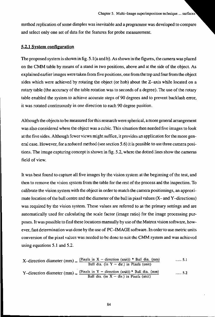
Chapter 5. Multi-Image superimposition technique ... <lIr£"o,"<
method replication of some dimples was inevitable and a programme was developed to compare
and select only one set of data for the features for probe measurement.
5.2.1 System configuration
The proposed system is shown in fig. 5.1 (a and b). As shown in the figures, the camera was placed
on the CMM table by means of a stand in two positions, above and at the side of the object. As
explained earlier images were taken from five positions, one from the top and four from the object
sides which were achieved by rotating the object (or hob) about the Z-axis while located on a
rotary table (the accuracy of the table rotation was to seconds of a degree). The use of the rotary
table enabled the system to achieve accurate steps of 90 degrees and to prevent backlash error,
it was rotated continuously in one direction to each 90 degree position.
Although the objects to be measured for this research were spherical, a more general arrangement
was also considered where the object was a cubic. This situation then needed five images to look
at the five sides. Although fewer views might suffice, it provides an application for the more gen
eral case. However, for a reduced method (see section 5.6) it is possible to use three camera posi
tions. The image capturing concept is shown in fig. 5.2, where the dotted lines show the cameras
field of view.
It was best found to capture all five images by the vision system at the beginning of the test, and
then to remove the vision system from the table for the rest of the process and the inspection. To
calibrate the vision system with the object in order to match the camera positionings, an approxi
mate location of the ball centre and the diameter of the ball in pixel values (X- and Y -directions)
was required by the vision system. These values are referred to as the primary settings and are
automatically used for calculating the scale factor (image ratio) for the image processing pur
poses. It was possible to find these locations manually by use of the Matrox vision software, how
ever, fast determination was done by the use of PC-IMAGE software. In order to use metric units
conversion of the pixel values was needed to be done to suit the CMM system and was achieved
using equations 5.1 and 5.2.
X-direction diameter (mm) = (Pixels in X - direction (unit» • Ball dia. (mm) Ball dia. (in Y - dir.) in Pixels (unit)
Y -direction diameter (mm) = (Pixels in Y - direction (unit))' Ball dia. (mm) Ball dia. (in X - dir.) in Pixels (unit)
84
...... 5.1
...... 5.2
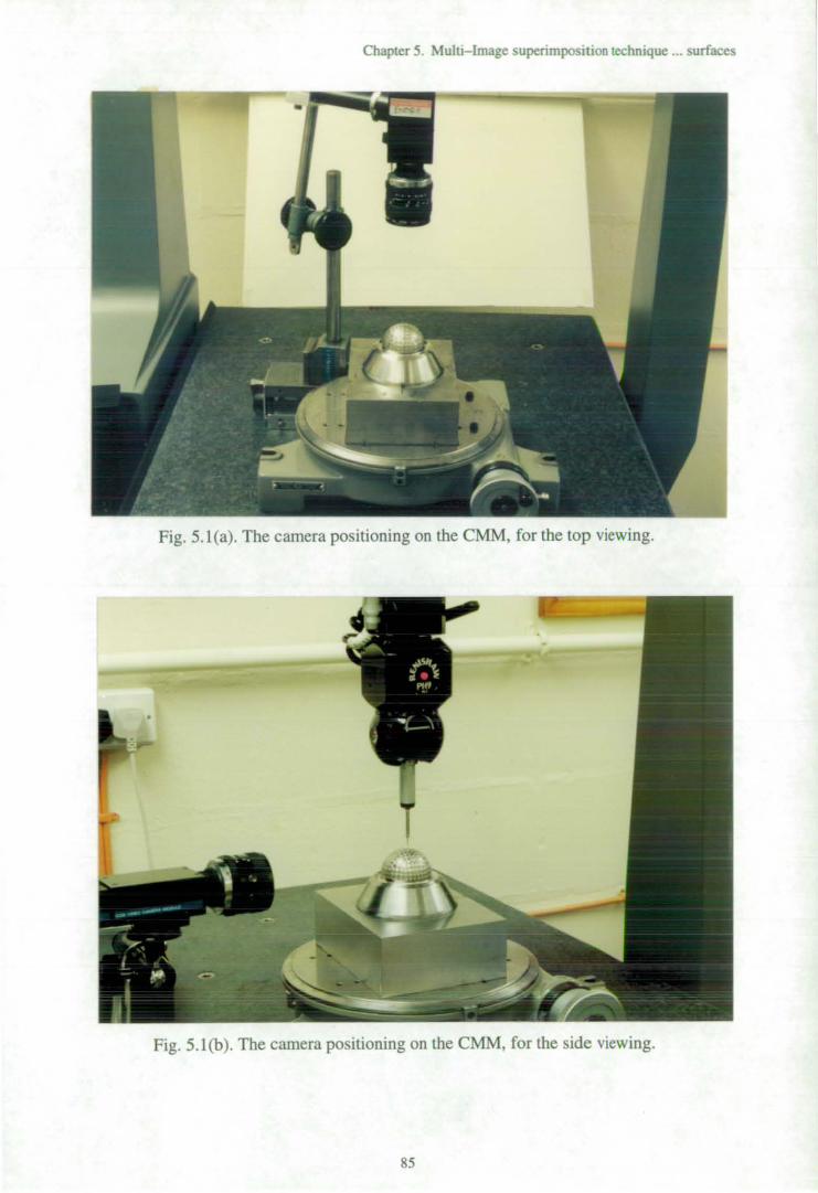
Chapter 5. Multi-Image superimposition technique ... surfaces
Fig. S.l(a). The camera positioning on the CMM, for the top viewing.
Fig. 5.1 (b). The camera positioning on the CMM, for the side viewing.
85
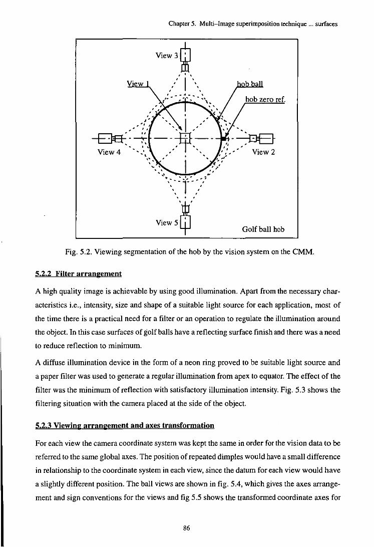
Chapter 5. Multi-Image superimposition technique ... surfaces
View3~ , ' , , I ' , , , , , ,
,. . , ' ~ .. , ,
, , , I
-EJa-' " - - ---T-. ' , . "
View 4
~ , . , .. "''','' .. : 1 .. ' ... · ...... ",'
, , , , , , , , ,
J!t View 5ltJ
-~ If ,J-...J'1....... , ' ,
View 2
Golf ball hob
Fig. 5.2. Viewing segmentation of the hob by the vision system on the CMM.
5.2.2 Filter arrangement
A high quality image is achievable by using good illumination. Apart from the necessary char
acteristics i.e., intensity, size and shape of a suitable light source for each application, most of
the time there is a practical need for a filter or an operation to regulate the illumination around
the object. In this case surfaces of golf balls have a reflecting surface finish and there was a need
to reduce reflection to minimum.
A diffuse illumination device in the form of a neon ring proved to be suitable light source and
a paper filter was used to generate a regular illumination from apex to equator. The effect of the
filter was the minimum of reflection with satisfactory illumination intensity. Fig. 5.3 shows the
filtering situation with the camera placed at the side of the object.
5.2.3 Viewing arrangement and axes transformation
For each view the camera coordinate system was kept the same in order for the vision data to be
referred to the same global axes. The position of repeated dimples would have a small difference
in relationship to the coordinate system in each view, since the datum for each view would have
a slightly different position. The ball views are shown in fig. 5.4, which gives the axes arrange
ment and sign conventions for the views and fig 5.5 shows the transformed coordinate axes for
86
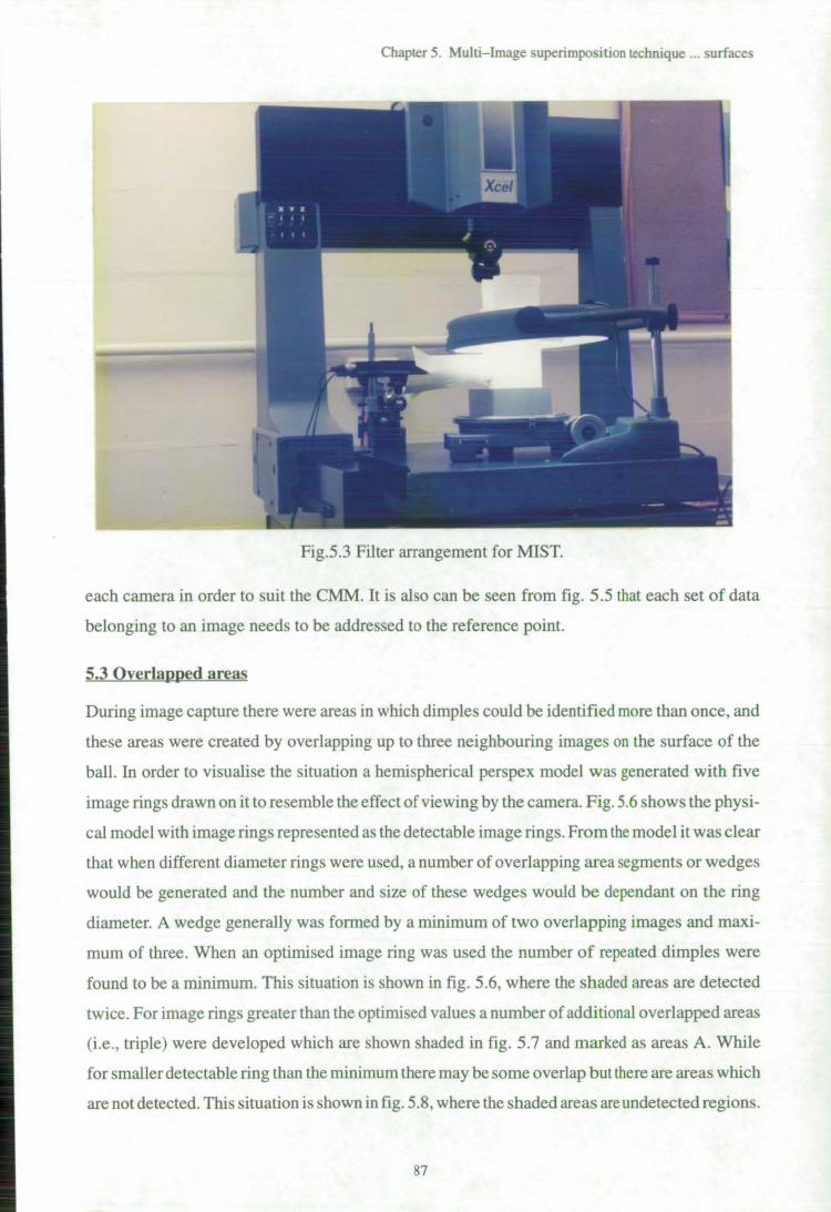
Chapter 5. Multi-Image superimposition technique ... surfaces
Fig.5.3 Filter arrangement for MIST.
each camera in order to suit the CMM. It is also can be seen from fig. 5 .5 that each set of data
belonging to an image needs to be addressed to the reference point.
5.3 Overlapped areas
During image capture there were areas in which dimples could be identified more than once, and
these areas were created by overlapping up to three neighbouring images on the surface of the
ball. In order to visualise the situation a hemispherical perspex model was generated with five
image rings drawn on it to resemble the effect of viewing by the camera. Fig. 5.6 shows the physi
cal model with image rings represented as the detectable image rings. From the model it was clear
that when different diameter rings were used, a number of overlapping area segments or wedges
would be generated and the number and size of these wedges would be dependant on the ring
diameter. A wedge generally was formed by a minimum of two overlapping images and maxi
mum of three. When an optimised image ring was used the number of repeated dimples were
found to be a minimum. This situation is shown in fig. 5.6, where the shaded areas are detected
twice. For image rings greater than the optirnised values a number of additional overlapped areas
(i.e., triple) were developed which are shown shaded in fig. 5.7 and marked as areas A. While
for smaller detectable ring than the minimum there may be some overlap but there are areas which
are not detected. This situation is shown in fig. 5.8, where the shaded areas are undetected regions .
87
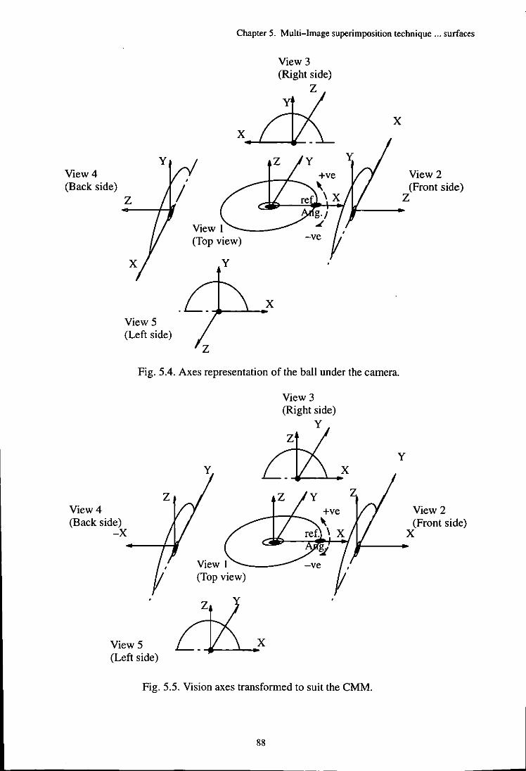
View 4 (Back side)
z
View 5 (Left side)
Chapter 5. Multi-Image superimposition technique ... surfaces
View 3 (Right side)
Z y
x._'--_~
View 1 (Top view)
y
x
View 2 (Front side)
Z
Fig. 5.4. Axes representation of the ball under the camera.
View 4 (Back side)
-x
View 5 (Left side)
View 1 (Top view)
View 3 (Right side)
y
z
Fig. 5.5. Vision axes transformed to suit the CMM.
88
y
View 2 (Front side)
X
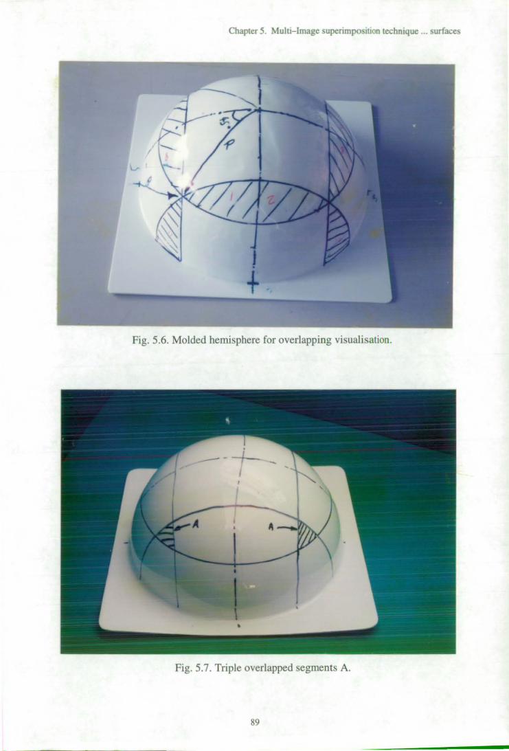
Chapter 5. Multi-Image superimposition technique ... surfaces
Fig. 5.6. Molded hemisphere for overlapping visualisation.
Fig. 5.7. Triple overlapped segments A.
89
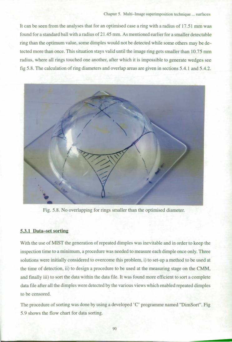
Chapter 5. Multi-Image superimposition technique ... surfaces
It can be seen from the analyses that for an optimised case a ring with a radius of 17.51 mm was
found for a standard ball with a radiu of21.45 mm. As mentioned earlier for a smaller deteclable
ring than the optimum value, some dimples would not be detected while some others may be de
tected more than once. This situation stays valid until the image ring gets smaller than 10.75 mm
radius, where all rings touched one another, after which it is impossible to generate wedges see
fig 5.8. The calculation of ring diameters and overlap areas are given in sections 5.4.1 and 5.4.2.
Fig. 5.8. No overlapping for rings smaller than the optimised diameter.
5,3,1 Data-set sorting
With the use of MIST the generation of repeated dimples was inevitable and in order to keep the
in pection time to a minimum, a procedure was needed to measure each dimple once only. T hree
solutions were initially considered to overcome this problem, i) to set-up a method to be used at
the time of detection, ii) to design a procedure to be used at the measuring stage on the CMM,
and finally iii) to sort the data within the data file. It was found more efficient to sort a complete
data file after all the dimples were detected by the various views which enabled repeated dimples
to be censored.
The procedure of sorting was done by using a developed 'C' programme named "DimSort". Fig
5.9 shows the flow chart for data sorting.
90
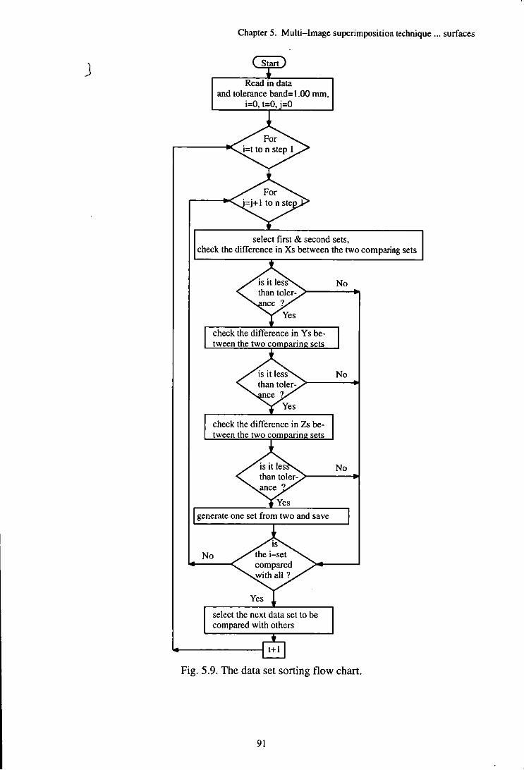
J
Chapter 5. Multi-Image superimposition technique ... surfaces
Read in data and tolerance band= 1.00 mm,
i=O, t=O, '=0
select first & second sets, check the difference in Xs between the two comparing sets
check the difference in Y s be-
check the difference in Zs between the two corn arin sets
generate one set from two and save
No
select the next data set to be compared with others
No
No
No
Fig. 5.9. The data set sorting flow chart.
91

Chapter 5. Multi-Image superimposition technique ... surfaces
The programme starts by reading in dimple data and placing it in a 3-D array. Each set of dimple
coordinates is compared with others in order to find matched values within specified tolerance
bands.
The tolerance band would vary with the golf ball type since they may have II different dimple
chord diameters [9]. However, a 1.00 mm tolerance band was found to be acceptable for the ma
jority of dimples. With a small amount of practice the most suitable band could be found for a
particular ball. If the tolerance was too small there was a risk of loosing some dimples. The com
parison procedure continues in order to find other matching data since there could be more than
one repeated set. It was found that averaging the repeated data sets was the best method to obtain
the dimple centre to be used by the CMM. Once a complete set of data was obtained it was stored
in a file for further consideration.
Various golf balls were tested using the above method with the machine under continuous
supervision in order to check the amount of the repeated data for different tolerance bands. Dur
ing the tests the original data from the MIST was continuously checked against the sorted file in
order to asses the effect of the identification process for the repeated dimples, and also to evaluate
the averaging method of the repeated data. Up to 90 per cent of the repeated data was detected
and an average value substituted leaving the remaining 10 per cent to be measured more than
once.
5.4 Mathematical evaluation of the overlapped areas
In order to minimise the number of repeated dimples from various views the size of the identifica
tion zone needs to be optimised. Experience has shown that they can be considered to be approxi
mately circular in shape and therefore to develop a mathematical solution, circular identification
zones or rings have been assumed. The procedure of calculating the detectable ring is shown in
the next section and two methods were developed for calculating the identification zone. The first
method uses an approximate evaluation and the second method follows a surface calculation
[104,105,106]. The use of the approximation method also made it possible to speculate on an
answer for the zone area. Once the detectable ring was identified the total area for five captured
images was calculated and used to determine the overlapped area ratio to the ball surface from
which the amount of repeated dimples can be identified.
5.4.1 Calculation of the detectable ring diameter for optimum overlap
In order to achieve optimum overlap when the MIST was applied to a sphere it was necessary
to calculate the radius of the detectable ring (i.e., RI) on a half hemisphere. This was done by
92
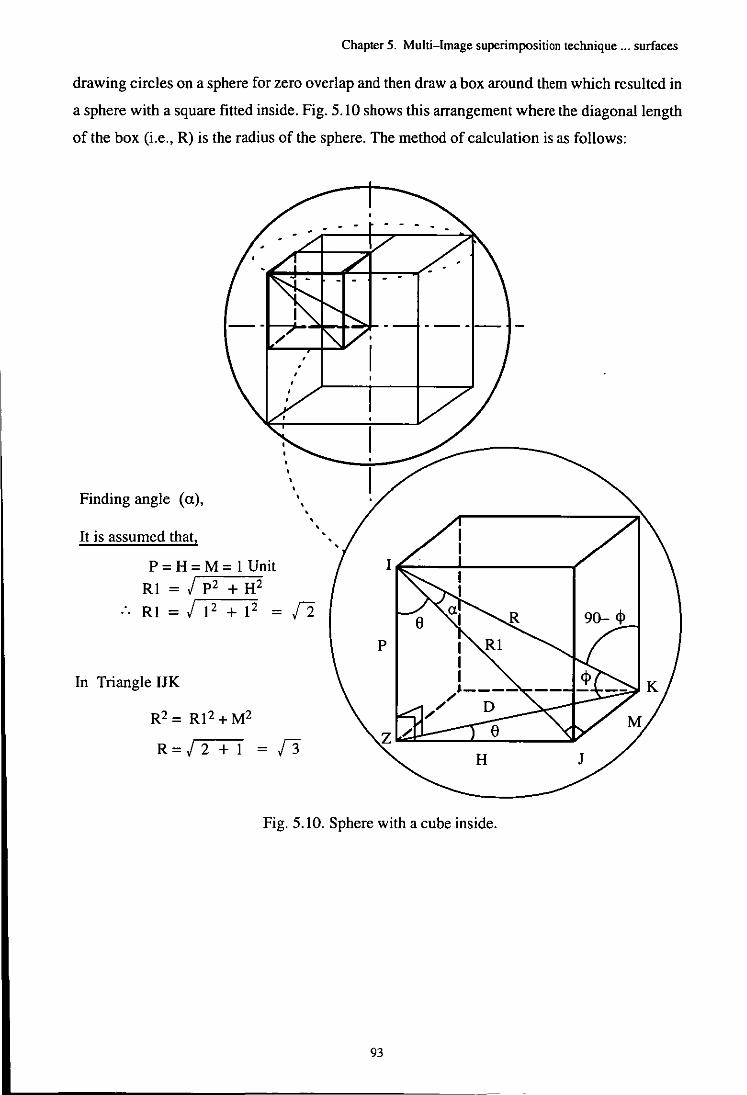
Chapter 5. Multi-Image superimposition technique ... surfaces
drawing circles on a sphere for zero overlap and then draw a box around them which resulted in
a sphere with a square fitted inside. Fig. 5.10 shows this arrangement where the diagonal length
of the box (i.e., R) is the radius of the sphere. The method of calculation is as follows:
Finding angle (a),
It is assumed that,
P = H = M = I Unit RI = j p2 + H2
• •
.. RI = j 12 + 12 = [2
In Triangle IJK
R2 = R12 + M2
R= j 2 + 1 = [3
I~--~~--------~
p
Fig. 5.10. Sphere with a cube inside.
93
90- <j>
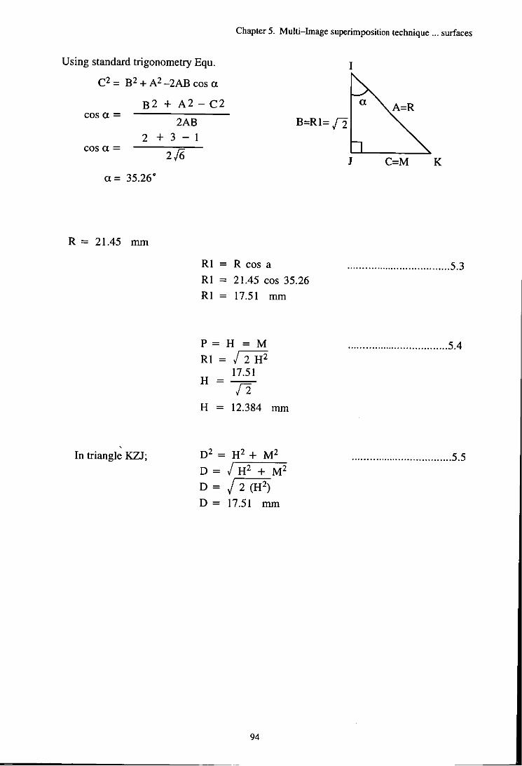
Chapter 5. Multi-Image superimposition technique ... surfaces
Using standard trigonometry Equ. I
C2 = B2 + A2_2AB cos 0.
cos 0. = B2 + A2 - C2
2AB B=RI=[2 2 + 3 - I
cos 0. = 2./6 0. = 35.26°
R = 21.45 mm
In triangle KZJ;
RI = R cos a
RI = 21.45 cos 35.26
RI = 17.51 mm
J C=M K
................................... 5.3
P = H = M ................................ ..5.4 RI = j 2 H2
17.51 H = [2
H = 12.384 mm
0 2 = H2 + M2
0= j H2 + M2
0= j 2 (H2)
0= 17.51 mm
94
.................................. 5.5
Chapter 5. Multi-Image superimposition technique ... surfaces
Total detected area for 5 images using the detectable ring
The total area for five images by the use of the detectable ring can be calculated by following
method.
Top view
Side view
Detectable ring dia. = 17.51 mm
Area = 21tR2
= 21t(l7.51)2
= 1926.42 mm2
Area = 21tR2
2it17.51)2 =
2 = 963.21 mm2
Total areas for 5 images Total areas = Top view + 4 X (Side view)
= 1926.42 + 4(963.21)
= 5779.27 mm2
95
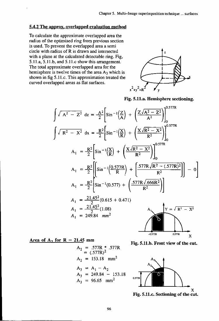
Chapter 5. Multi-Image superimposition technique ... surfaces
S.4.2 The approx. overlapped evaluation method
To calculate the approximate overlapped area the radius of the optimised ring from previous section is used. To prevent the overlapped area a semi circle with radius of R is drawn and intersected with a plane at the calculated detectable ring. Fig, 5.1 La, 5.ll.b, and 5.ll.c show this arrangement. The total approximate overlapped area for the hemisphere is twelve times of the area A3 which is shown in fig 5.II.c. This approximation treated the curved overlapped areas as flat surfaces.
z
Fig. S.U.a. Hemisphere sectioning.
_ Z2 dz = ~2[Sin-I(~) + (ZJA:2- Z2)f77R
O.577R
X2 dx = ~2[Sin-IGD + (XJR~2- X2)t
Al = ~2[Sin-l(i) + (XJR~2- X2)I577R
Al = ~2[[Sin-I(0.5~7R) + ["577R R~~ (.577R)2 ] _ 0]
Al = ~2[Sin-I(0.577) + (-577R~i666R2)]
Al = 212452
(0.615 + 0.471)
Al = 212452
(1.08)
Al = 249.84 mm2
Area of A? for R = 21.45 mm
A2 = .577R * .577R = (.577R)2
A2 = 153.18 mm2
A3 = Al - A2 A3 = 249.84 - 153.18
A3 = 96.65 mm2
96
x Fig. S.lI.h. Front view of the cut.
x Fig. S.lI.c. Sectioning of the cut.
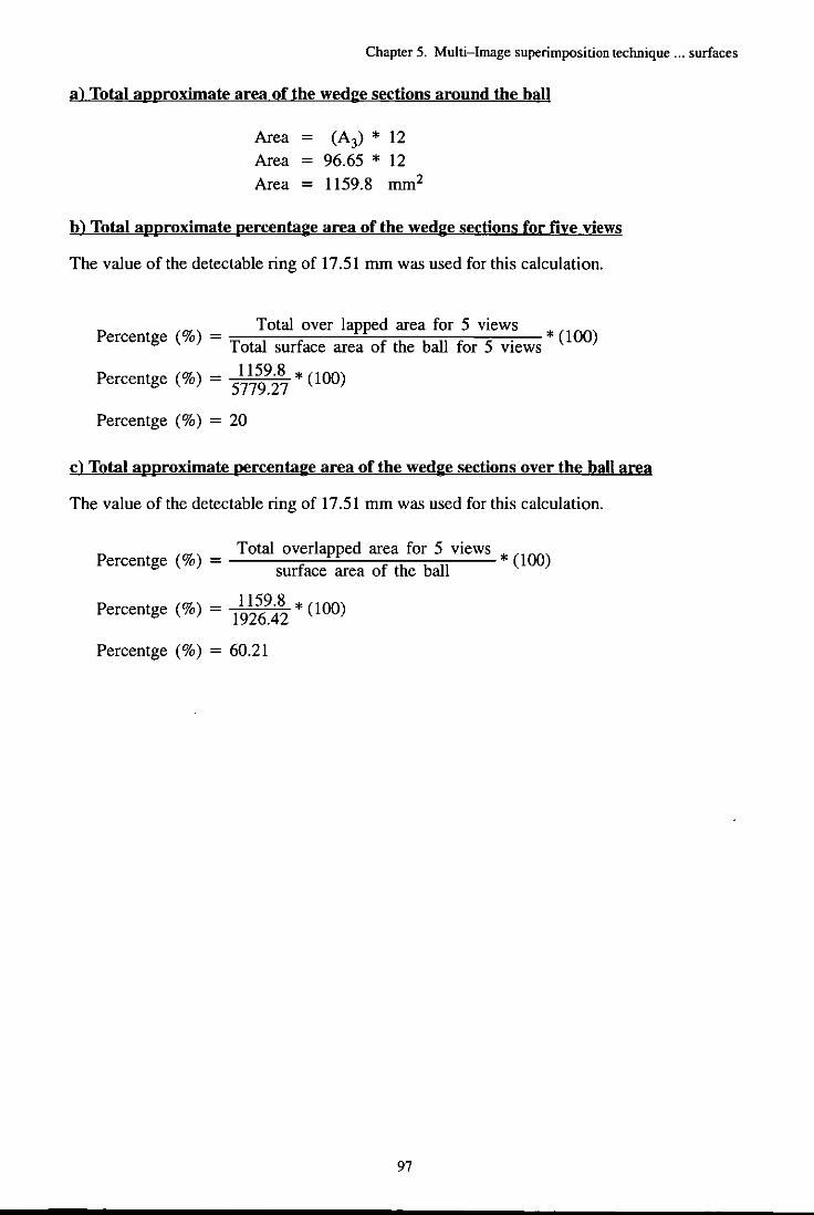
Chapter 5. Multi-Image superimposition technique ... surfaces
al Total approximate area of the wedge sections around the ball
Area (A3) * 12 Area = 96.65 * 12 Area = 1159.8 mm2
bl Total approximate percentage area of the wedge sections for five views
The value of the detectable ring of 17.51 mm was used for this calculation.
P 'il Total over lapped area for 5 views * 0 ercentge ( 0) = Total surface area of the ball for 5 views (I 0)
Percentge (%) = 5~~s:.i~ * (lOO)
Percentge (%) = 20
cl Total approximate percentage area of the wedge sections over the ball area
The value of the detectable ring of 17.51 mm was used for this calculation.
Total overlapped area for 5 views Percentge (%) = surface area of the ball * (lOO)
Percentge (%) = 1159.8 * (lOO) 1926.42
Percentge (%) = 60.21
97
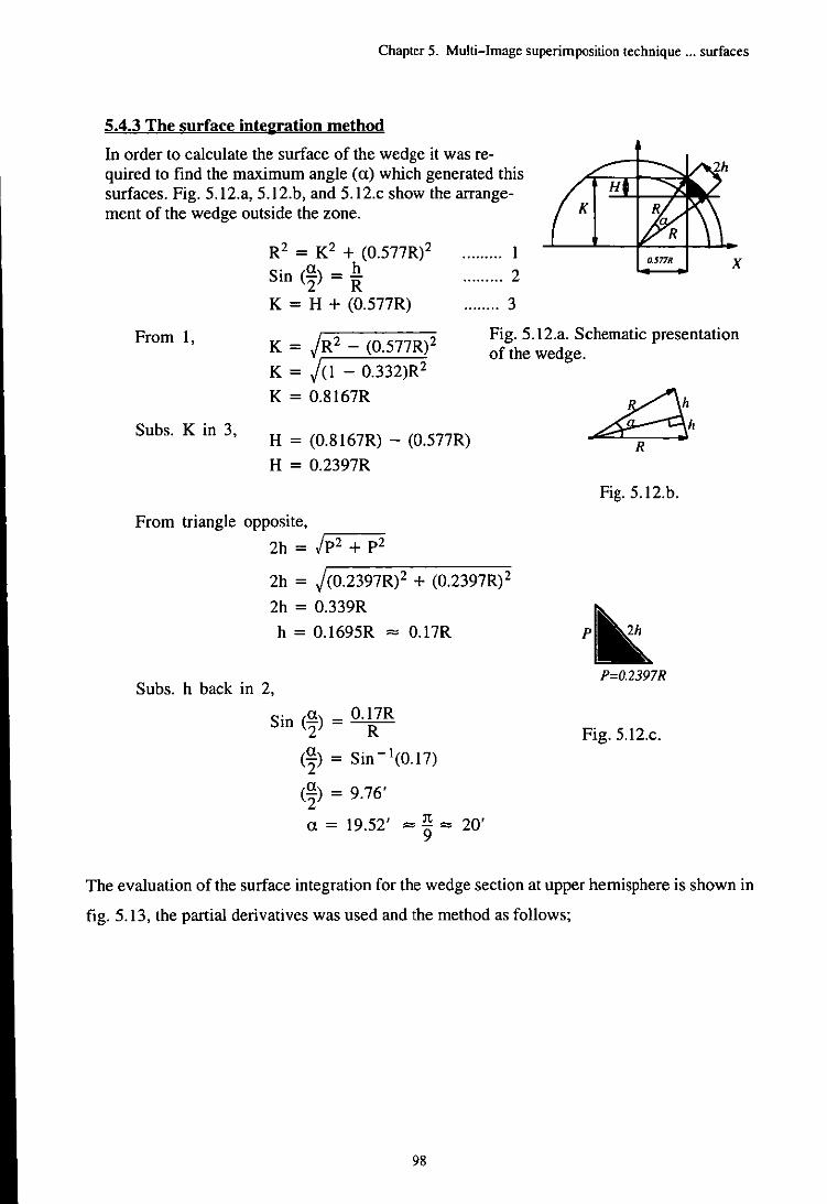
Chapter 5. Multi-Image superimposition technique ... surfaces
5.4.3 The surface integration method
In order to calculate the surface of the wedge it was required to find the maximum angle (a) which generated this surfaces. Fig. 5.12.a, 5.12.b, and 5.12.c show the arrangement of the wedge outside the zone.
R2 = K2 + (0.577R)2 Sin (a) = .!!
2 R K = H + (0.577R)
......... I ......... 2
........ 3
O.'77R x
From I, K = jR2 - (0.577R)2
K = j(1 - 0.332)R2
K = 0.8167R
Fig. 5.12.a. Schematic presentation of the wedge.
Subs. Kin 3, H = (0.8167R) - (0.577R)
H = 0.2397R
From triangle opposite,
2h = jp2 + p2
2h = j(0.2397R)2 + (0.2397R)2
2h = 0.339R
h = 0.1695R = 0.17R
Subs. h back in 2,
Sin (a) = O.17R 2 R
(~) = Sin -1(0.17)
(~) = 9.76'
a = 19.52' = ~ = 20'
Fig. 5.12.b.
P=O.2397R
Fig. S.12.c.
The evaluation of the surface integration for the wedge section at upper hemisphere is shown in
fig. 5.13, the partial derivatives was used and the method as follows;
98
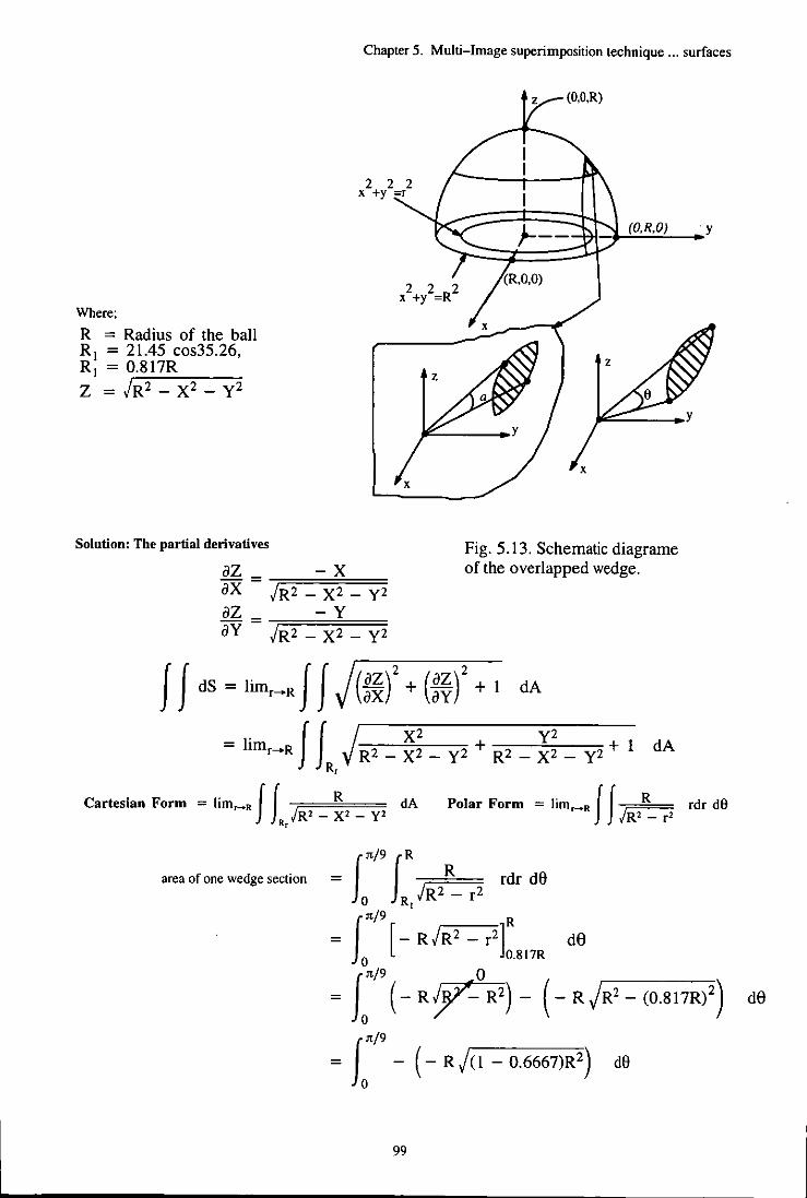
Where;
R = Radius of the baIl RI = 21.45 cos35.26, RI = O.817R Z = jr-R=:::2:":'_~X""""2-_-y-;:2
Solution: The partial derivatives
az = - X
Chapter 5. Multi-Image superimposition technique ... surfaces
(O,O,R)
(O,R,O) . y
Fig. 5.13. Schematic diagrame of the overlapped wedge.
ax jR2 _ X2 _ y2 az = - y ay JR2 _ x2 _ y2
Cartesian Form - lim f f R - ~R ./R' _ X'
R,
area of one wedge section =
=
=
=
dA Y'
Polar Form = lim~R f f R ./R' - r'
f/9 r JR2R_ r2
rdr de o RI
f/9 R [-RJR2 -r2] de
o O.817R
rdr de
f/9 0 o (- RF) - (- RjR2 - (o.817R)2)
f/9 (- Rj(l - o.6667)R2) de
99
de
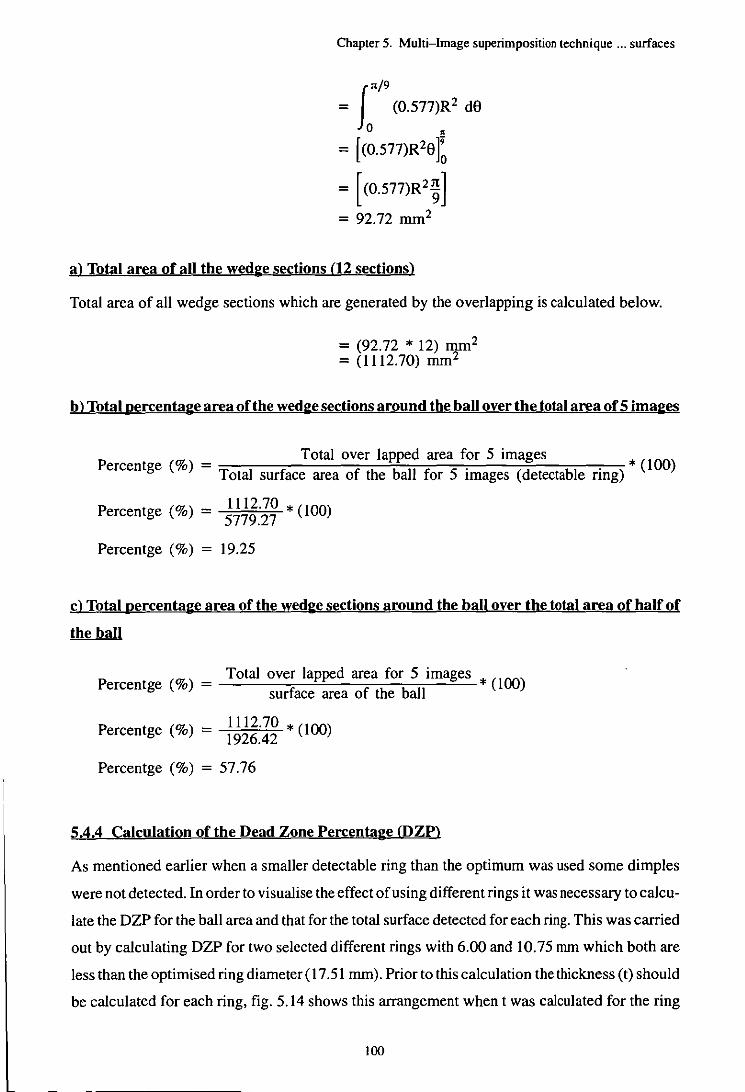
Chapter 5. Multi-Image superimposition technique ... surfaces
J"/9
= (0.577)R2 de
o • = [(0.577)R2e l: = [(0.577)R2~] = 92.72 mm2
a) Total area of all the wedge sections (12 sections)
Total area of all wedge sections which are generated by the overlapping is calculated below.
= (92.72 * 12) mm2
= (1112.70) mm2
b) Total percentage area ofthe wedge sections around the ball over the total area of 5 images
Total over lapped area for 5 images 00 Percentge (%) = .. * (I )
Total surface area of the ball for 5 Images (detectable f1ng)
Percentge (%) = 1112.70 * (100) 5779.27
Percentge (%) = 19.25
c) Total percentage area of the wedge sections around the ball over the total area of half of
the ball
Total over lapped area for 5 images Percentge (%) = surface area of the ball * (100)
Percentge (%) = 1112.70 * (lOO) 1926.42
Percentge (%) = 57.76
5.4.4 Calculation of the Dead Zone Percentage fDZP)
As mentioned earlier when a smaller detectable ring than the optimum was used some dimples
were not detected. In order to visualise the effect of using different rings it was necessary to calcu
late the DZP for the ball area and that for the total surface detected for each ring. This was carried
out by calculating DZP for two selected different rings with 6.00 and 10.75 mm which both are
less than the optimised ring diameter (17.51 mm). Prior to this calculation the thickness (t) should
be calculated for each ring. fig. 5.14 shows this arrangement when t was calculated for the ring
100
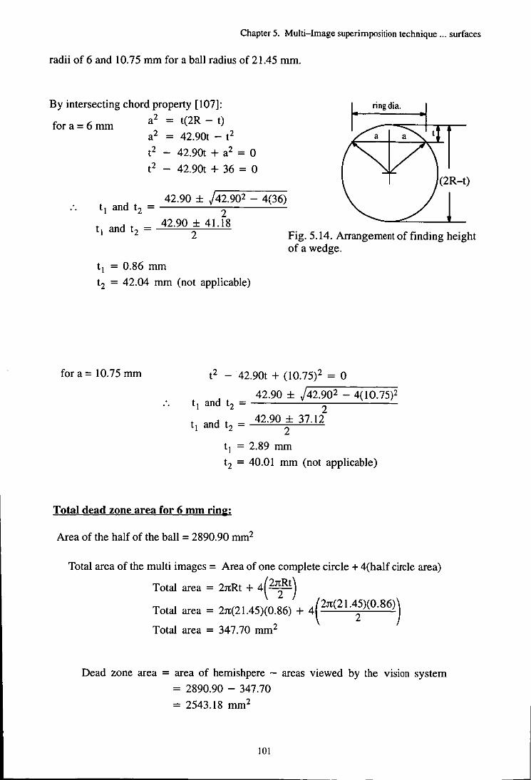
Chapter 5. Multi-Image superimposition technique ... surfaces
radii of 6 and 10.75 mm for a ball radius of 21.45 mm.
By intersecting chord property [107]: ring dia.
fora=6mm a2 = t(2R - t)
a2 = 42.9Ot - t2
t2 42.90t + a2 = 0
t2 42.9Ot + 36 = 0
t1 and t2 =
t1 and t2 =
42.90 ± /42.902 - 4(36) 2
42.90 ± 41.18 2 Fig. 5.14. Arrangement of finding height
ofa wedge.
t1 = 0.86 mm
t2 = 42.04 mm (not applicable)
for a = 10.75 mm t2 - 42.90t + (10.75)2 = 0 ,...-----.,.------,-
42.90 ± /42.902 - 4(10.75)2 t1 and t2 = 2
t1 and t2 = 42.90 i 37.12
t1 = 2.89 mm
t2 = 40.01 mm (not applicable)
Total dead zone area for 6 mm rim::
Area of the half of the ball = 2890.90 mm2
Total area of the multi images = Area of one complete circle + 4(haJf circle area)
Total area = 21tRt + 4e~Rt) Total area = 21t(21.45)(0.86) + 4C1t(21.~)(0.86)) Total area = 347.70 mm2
Dead zone area = area of hemishpere - areas viewed by the vision system
= 2890.90 - 347.70
= 2543.18 mm2
101
Chapter 5. Multi-Image superimposition technique ... surfaces
Dead zone area in percentage (%) :
Percentge (%) = il~~:~g * (lOO)
Percentge (%) = 87.97
The dead zone area for ring of 10.75 mm :
Total area of the multi image area's = Area of one complete circle + 4(half circle area)
Total area's = 23tRt + 4e~Rt) Total area's = 23t(21.45)(2.89) + 4(23t(21.4g)(2.89))
Total area's = 1168.49 mm2
Dead zone area = area of hemishpere - areas viewed by the vision system
= 2890.90 - 1168.49
= 1722.40 mm2
Dead zone area in percentage (%) :
Percentge (%) = i~~5:~g * (lOO)
Percentge (%) = 59.58
5.5 Experiments and results
Six different golf balls and two golf hobs were tested for feature deteciion and inspection by the
proposed method see table 5.1. For each ball and hob the MIST was applied, and a number of
different image rings were used and data files optimised by the use of the sorting method. The
golf balls were selected from a range of ball types on the market, including two yellow coloured
balls. From the table it can be seen that the Top Flite Magna SPALDING ball has an unusual de
sign and it was selected since it was believed that some dimples intersected and this is not a com
mon practice. The pattern on this ball is not designed from one of the Platonic shapes. However,
it is a type of segmented design which does not necessarily behave as if it were spherically sym
metrical. These balls all had spherical shaped dimples with various dimple chord diameters.
In order to analyse and compare the results between the balls a minimum area which would cover
a dimple pattern on each ball was selected. However, patterns on the die separation line were not
selected, since the dimples on this line may have been ground to remove excess plastic during
102
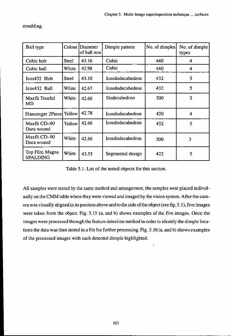
Chapter 5. Multi-Image superimposition technique ". surfaces
moulding.
Ball type Colour Diameter Dimple pattern No. of dimples No. of dimple of ball mm types
Cubic hob Steel 43.16 Cubic 440 4
Cubic ball White 42.98 Cubic 440 4
Icos432 Hob Steel 43.10 Icosdodecahedron 432 5
Icos432 Ball White 42.67 Icosdodecahedron 432 5
Maxfli Tourltd White 42.60 Dodecahedron 500 3 MD
Slanzenger 2Piece Yellow 42.78 Icosdodecahedron 420 4
Maxfli CD-90 Yellow 42.66 Icosdodecahedron 432 5 Dura wound
Maxfli CD-90 White 42.66 Icosdodecahedron 500 3 Dura wound
Top Flite Magna White 43.55 Segmented design 422 5 SPALDING
Table 5.1. List of the tested objects for this section.
All samples were tested by the same method and arrangement, the samples were placed individ
ually on the CMM table where they were viewed and imaged by the vision system. After the cam
era was visually aligned in its position above and to the side of the object (see fig. 5.1), five images
were taken from the object. Fig. 5.15 (a, and b) shows examples of the five images. Once the
images were processed through the feature detection method in order to identify the dimple loca
tions the data was then stored in a file for further processing. Fig. 5.16 (a, and b) shows examples
of the processed images with each detected dimple highlighted.
103
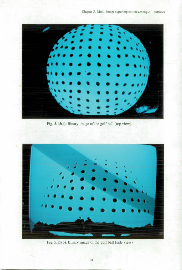
Chapter 5. Multi-Image superimposition technique ... surfaces
Fig. 5.15(a). Binary image of the golf ball (top view).
, , ,
Fig. 5.15(b). Binary image of the golf ball (side view).
104
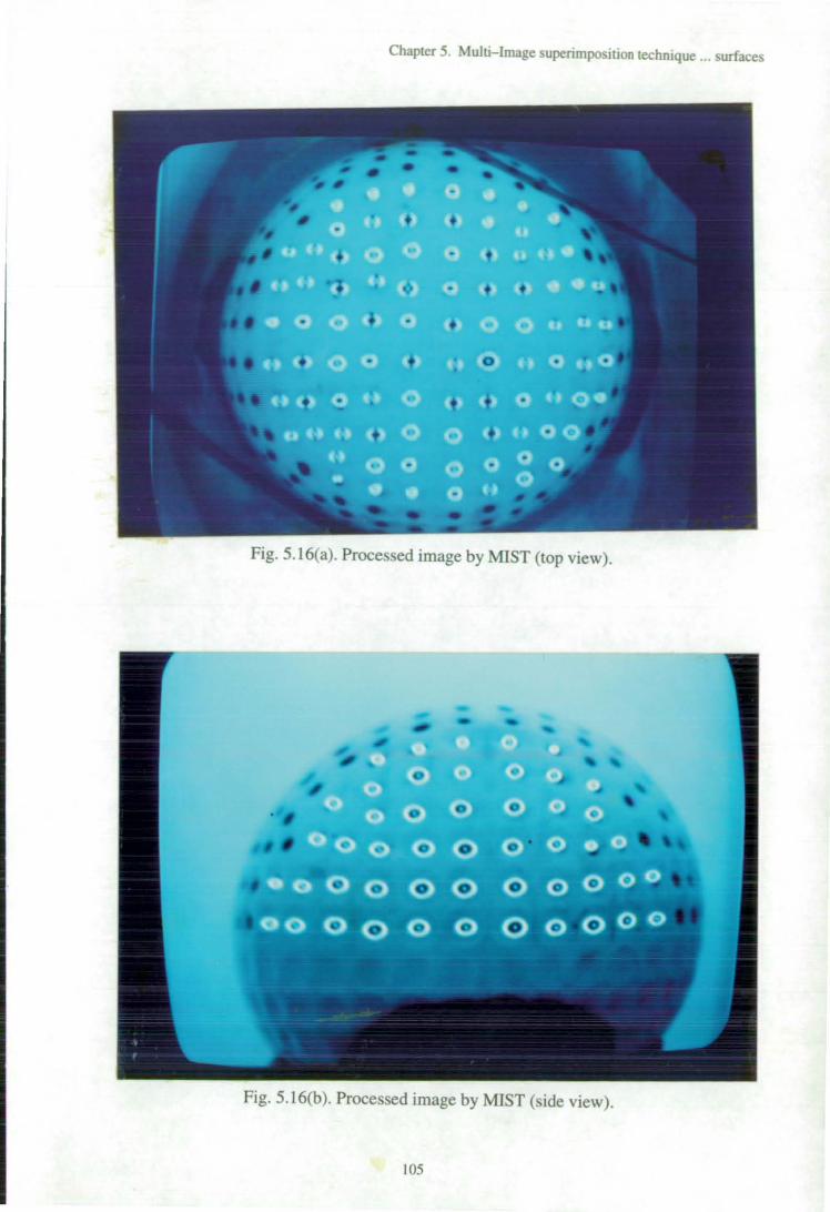
Chapter 5. Multi-Image superimposition technique ... surfaces
Fig. 5.16(a). Processed image by MIST (top view).
Fig. 5.16(b). Processed image by MIST (side view).
105
Chapter 5. Multi-Image superimposition technique ... surfaces
Each sorted data file was checked in order to determine the sorting process and a practical inspec
tion was conducted for the relevant dimples. In order to check the validity of the CMM probing
method three further methods were used on sample dimples to check shape and depth. One was
the Taylor Hobson Talylin, the second was Universal Measuring Machine MU214B, and the third
was laser scanner with the use of 3-D IsoSurf software.
The Talylin is an electronic instrument, capable of measuring surface finish and shape. The main
parts of the machine are a measuring head which consists of a stylus and a shoe, an electric motor
and a gearbox. The measuring head is drawn across the surface under test. The stylus and its arm
are part of a circuit such that when displaced by the surface irregularities during traversing, the
A.C. current flowing in the circuit modulates the amplitude. This is fed to an amplifier and causes
a pen recorder to produce a permanent record of the displacement. The system accuracy was +/-
0.2 microns with various magnifications.
The IsoSurf as a complete unit consists of three main parts, a distance measurement laser stylus
(RM600), a motion controller (DMC-I 000), and a 3-D software. The laser stylus is designed for
non contact measurements between 0.0 I !lm and 600 !lm. The equipment contains a sensor and
sensor interface and results are given to a four digit display and LED string. An infrared laser
beam (780 nm) is focused on the surface [108] to a spot of 2 or 4 !lm diameter, according to the
type of sensor, which is reflected back to a focus detector. This device is capable of sampling rates
of more than 500 per second. It can be interfaced to a variety of motors and drives. This controller
provides several modes of motion for the laser stylus including gearing and user defined path fol
lowing. The system accuracy was +/- 5 microns.
The MU-214B machine [109] is an optical device frequently used for measuring workpieces pro
duced in small batches. The measuring range (graduated length of the standard scale) is 75mm.
Readings to 0.0005 mm, are made by means of the micrometer microscope fixed to the right hand
side of the transverse carriage, while the sensitivity of the settings was 2 !lm. In this case the dim
ple chord diameter (distance between the two edges) was inspected through horizontal displace
ment of the machine table which carried the locating microscope and by accurate focusing of the
latter on the edge of a dimple. The measurement of the dimple depth was subjective since there
was no guaranteed way of locating the dimple centre under the optical head. The chord diameters
of a few dimples were measured accordingly by the Talylin and the MU-214B. The laser scanner
was used as an alternative to check on selected dimples in order to check profile and shape. How
ever, the amount of time and effort required for using the laser device with its limitation on the
range of measurement made it less attractive. The table 5.2. shows the results of these tests on
106
Chapter 5. Multi-Image superimposition technique ... surfaces
dimple chord diameter, where the bold figures show the maximum and minimum values found
for each sample dimple measured by four measuring systems.
Sample No:
Ball type TesaCMM Talylin MU-214B Laser Scanner Max. variation
1 Icos432 4.108 4.064 3.978 4.030 0.130
2 Icos432 3.986 4.062 3.967 4.120 0.153
3 Icos432 4.049 4.166 3.966 4.002 0.200
4 Icos432 4.044 4.064 4.028 4.000 0.064
5 Icos432 3.973 4.160 4.033 4.010 0.187
6 Icos432 3.998 4.120 4.010 4.025 0.122
Table 5.2. Dimple chord measurement results on sampled dimples.
The maximum variation in chord diameter is 0.2 mm which compares favourably with the CMM
measurements, since the positioning of the dimple under the instrument at its centre is subjective.
The MIST was practically applied to the selected balls and, the sum of detected dimples for
example on half of a cubic ball was 220 which is 100 per cent. When different detectable rings
were applied to the ball, an increase in the number of dimples was detected, consequently differ
ent ratios were attempted, table 5.3 shows results of these tests.
Detectable ring Number of Percentage (%) diameter (mm) dimple detected (Detected dimPles)
220
15.00 167 76%
17.00 223 106%
17.50 240 109%
18.00 254 115.5%
18.50 273 124.1 %
Table 5.3. Results for different detectable ring diameter on a cubic ball.
From the results it was possible to compare the ratio of detected dimples with the detectable ring
diameter, for example a larger detectable ring will allow repeated detection of some dimples.
Also from the table it can be seen it is not possible to determine an exact ring size in order to have
100 per cent detected dimples. The system will generally give more or less than the optimum
value, the orientation of the ball, and the dimple markings i.e., size and the location in the dimple
have a considerable influence.
107
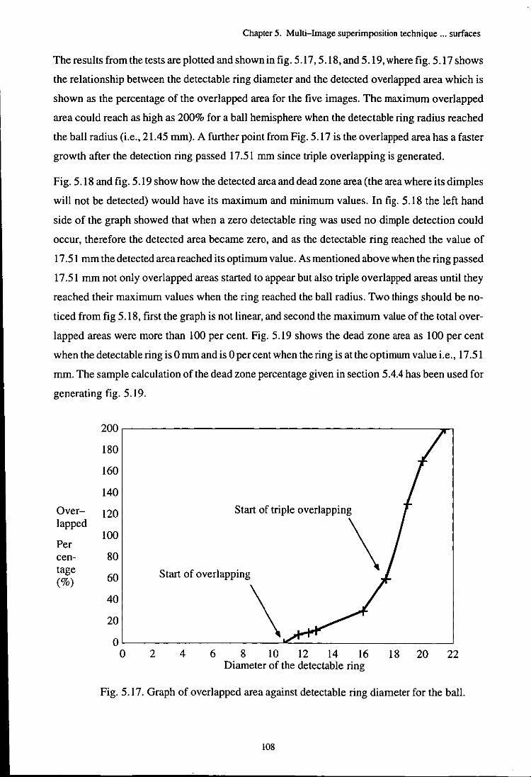
Chapter 5. Multi-Image superimposition technique ... surfaces
The results from the tests are plotted and shown in fig. 5.17, 5.18, and 5.19, where fig. 5.17 shows
the relationship between the detectable ring diameter and the detected overlapped area which is
shown as the percentage of the overlapped area for the five images. The maximum overlapped
area could reach as high as 200% for a ball hemisphere when the detectable ring radius reached
the ball radius (i.e., 21.45 mm). A further point from Fig. 5.17 is the overlapped area has a faster
growth after the detection ring passed 17.51 mm since triple overlapping is generated.
Fig. 5.18 and fig. 5.19 show how the detected area and dead zone area (the area where its dimples
will not be detected) would have its maximum and minimum values. In fig. 5.18 the left hand
side of the graph showed that when a zero detectable ring was used no dimple detection could
occur, therefore the detected area became zero, and as the detectable ring reached the value of
17.51 mm the detected area reached its optimum value. As mentioned above when the ring passed
17.51 mm not only overlapped areas started to appear but also triple overlapped areas until they
reached their maximum values when the ring reached the ball radius. Two things should be no
ticed from fig 5.18, first the graph is not linear, and second the maximum value of the total over
lapped areas were more than 100 per cent. Fig. 5.19 shows the dead zone area as 100 per cent
when the detectable ring is 0 mm and is 0 per cent when the ring is at the optimum value i.e., 17.51
mm. The sample calculation of the dead zone percentage given in section 5.4.4 has been used for
generating fig. 5.19.
200
180
160
140
Over- 120 Start of triple overlapping lapped
100 Per cen- 80 tage
60 (%)
40
20
\ Start of overlapping
\ 0
0 2 4 6 8 10 12 14 16 18 20 22 Diameter of the detectable ring
Fig. 5.17. Graph of overlapped area against detectable ring diameter for the ball.
108
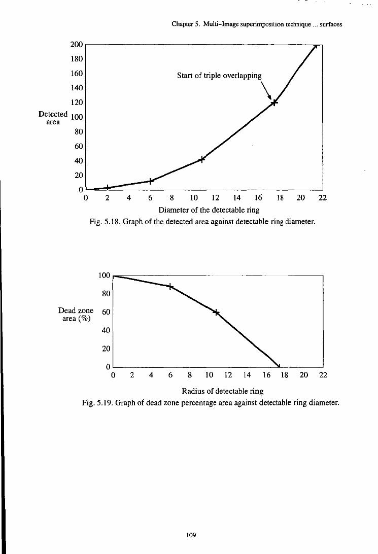
Chapter 5. Multi-Image superimposition technique ... surfaces
200
180
160 Start of triple overlapping
140
120 \
Detected 100 area
80
60
40
20
0 0 2 4 6 8 10 12 14 16 18 20 22
Diameter of the detectable ring
Fig. 5.18. Graph of the detected area against detectable ring diameter.
100
80
Dead zone 60 area (%)
40
20
0 0 2 4 6 8 10 12 14 16 18 20 22
Radius of detectable ring
Fig. 5.19. Graph of dead zone percentage area against detectable ring diameter.
109
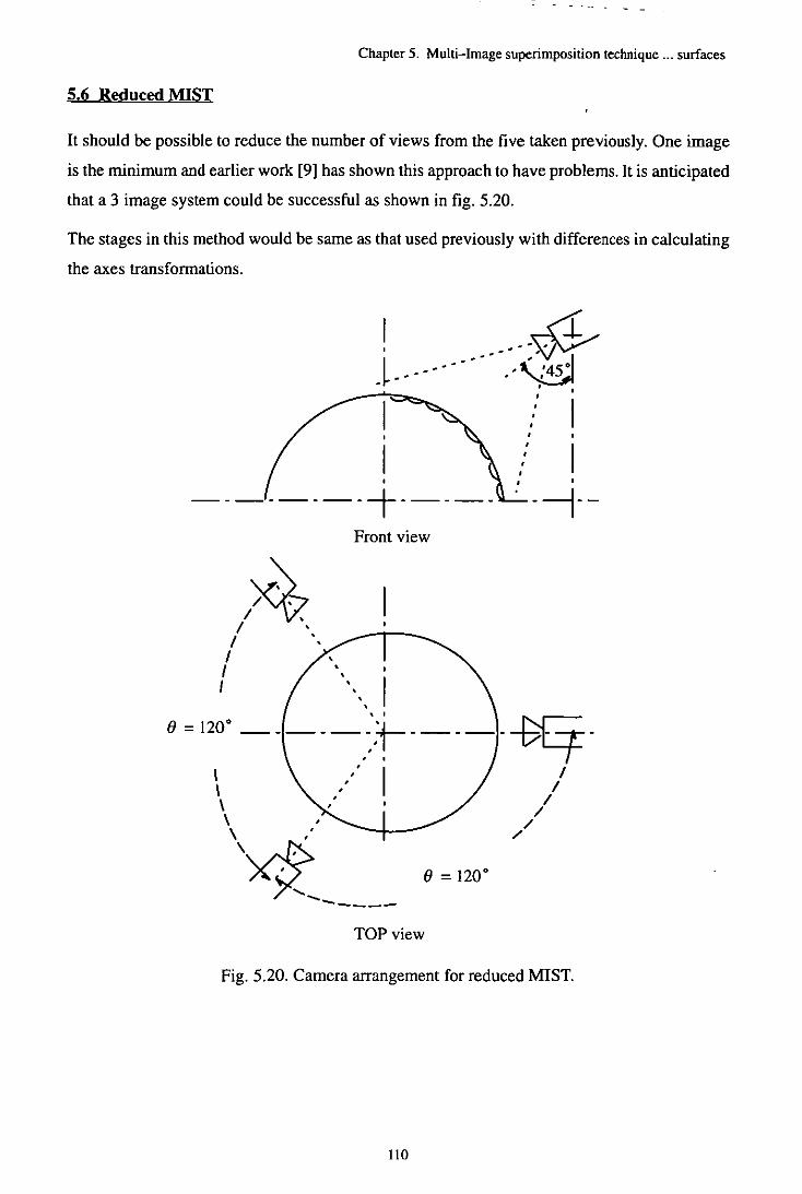
Chapter 5. Multi-Image superimposition technique ... surfaces
5.6 Reduced MIST
It should be possible to reduce the number of views from the five taken previously. One image
is the minimum and earlier work [9] has shown this approach to have problems. It is anticipated
that a 3 image system could be successful as shown in fig. 5.20.
The stages in this method would be same as that used previously with differences in calculating
the axes transformations.
I _~~ J------------.-. ~ ,
I : I , '
I .... I , " --------+----- . --i--
;>: /~
I ' / '
/
Front view
I I , I
() = 1200 -----~,+------~-" vI
\ ' I / \ I \ I \ //
\~" / () = 120 0
.......... -----TOP view
Fig. 5.20. Camera arrangement for reduced MIST.
110

Chapter 5. Multi-Image superimposition technique ... surfaces
5.7 Discussion
A one camera multi-image superimposed technique for surface feature identification has been
discussed in this chapter. Although the technique was applied to spherical shapes, the concept can
be studied, modified, and applied for non regular shapes.
The method used a one camera arrangement for the side views and also for the top view, while
the object was placed on a rotary table, however, the technique could easily have used five camer
as positioned around the workpiece at any location and the images fed into the vision computer
system.
The common problem of illuminating an object which sometimes develops the most challenging
section of a vision application has been solved by using a paper filter around the object of interest
which resulted in a uniform illumination.
Applying the MIST to spherical shapes generated areas which double overlapped and in certain
sections triple overlapped (sections A in fig. 5.7). The features in these areas will be detected two
or three times. In order to minimise these areas, and consequently the amount of repeated data,
a series of algorithms were developed. In addition to support the practical tests the overlapped
areas were analysed mathematically.
III

Chapter 6. The system error model
CHAPTER 6
THE SYSTEM ERROR MODEL
6.0 Introduction
The importance of dimple location on golf balls originated from their effect on the flight of the
ball. Size and shape inconsistency, positional inaccuracy and non symmetrical patterns are the
main factors which would generate unexpected flight behaviour. In this research the mentioned
manufacturing system errors were evaluated through the inspection of different (actual) hobs and
golf balls. Once the actual dimple locations are determined it is necessary to determine the posi
tional error. Each dimple will have an error with respect to its nominal position, however the error
determined will be with respect to the set up position for measurement. Clearly if the datum plane
is moved the error values will change. A method is required, which once the relative dimple posi
tions are measured, will realign the datum plane to give the minimum error. At present the posi
tional accuracy of dimples on tools and balls is assessed primarily through visual inspection and
by practical testing of a number of balls from the pre production models in the field.
To obtain the minimised positional error for the dimples there are a number of methods from
which a solution could be achieved. Some of these methods are capable of best fitting data to some
geometrical features e.g., least squares best fit or interpolation method to handle data in the form
of simultaneous algebraic equations in engineering using matrix notation. Mathematical sol
utions are also useful methods for minimising or maximising equations. They deal with functions
of several variables for example to the 'm' power under a prescribed set of constraints from which
the minimum or maximum points or coordinates can be calculated. The significant factor when
using these methods is that the data must be represented by a function [11 0].
The error analysis method for dimple patterns needed to deal with n variables in 3-D space where
there may not be an established function between the coordinates. In addition there is unlikely
to be a pattern for errors at each coordinate, which makes it difficult since each error should be
calculated individually, then compared with others and should satisfy a restricted pattern. It is
unlikely that the solution for these problems could ever follow a deterministic equation due to
uncertainties of the errors and their nature, however, a more iterative optimised approach could
lead to a satisfactory solution.
6.1 Review on error evaluation methods
For any measurement to be of use there are two main criteria which must be satisfied, the
rneasurement must use a system which is recognised and used by others in the field of application
112
Chapter 6. The system error model
(e.g, the International System of Units, ISO); and the degree of accuracy of the measurement must
be known. It is inevitable to have errors, however, a system of evaluating differences (errors)
should appreciate the type and source and should make appropriate compensation if necessary.
The British Standard BS5233 [Ill] (Glossary oftenns used in metrology), section five considers
the errors in two broad groups; errors in the results of measurements and errors of measuring in
struments. Regardless of the sources of error there are many fonnal methods which can be used
to evaluate and control error magnitude. They all aim to explain a sensible correlation between
inconsistency or variations of data in tests with a model or specification.
Many researchers have developed methods and algorithms to model and analyse geometric error
tolerance zones with the use of statistical analyses. They analysed and developed methods for
engineering features such as holes, flat surfaces, surfaces of tooth gears etc. Although much work
has been done there is little concentrated effort in any particular direction, some examples which
have been tried are as follows:-
Lehtihet and Gunasena [112] discussed solutions for idealised statistical models for the relation
ship between the position tolerance specification of a single hole and production errors. They
considered drilled holes in a flat plate, and used a series of statistical tests on the measured values
which were taken by a CMM, to describe production errors and the position tolerance of a hole
with regard of feature size and maximum material condition. Wang [113] developed a method
to detennine fonn feature tolerances of a machined part with sampled measurement points from
a CMM and evaluated the minimum tolerance zone as a constrained optimisation problem with
continuous functional relationships. He used a general purpose algorithm for constrained nonlin
ear optimisation, based on iterative fonnulation (explained in section 6.3.2). Elmaraghy et al.
[114,115] used a similar concept to evaluate and detennine actual geometric tolerances using
CMM measured data. They developed a procedure for systematic comparison of geometric vari
ations of measured features with their specified geometric tolerances by the use of algorithms and
nonlinear numerical optimisation techniques to fit the data to the minimum tolerance zone on the
surface of a cylindrical feature. They analysed measurement data by the use of point to point
measurement ratherthan curve fitting. The optimisation algorithm detennined the location of the
centre point, or reference axis of the geometric element (i.e., cylinder) from which the calculation
of the actual geometric tolerances was possible.
Litvin et al. [116] developed a method to minimise gear tooth surface deviations between the
theoretical and real surfaces for the improvement of precision. They used a least square method
to minimise the surface deviation in the direction of the nonnal to the theoretical surface.
1t3
Chapter 6. The system error model
There are other studies which analyse volumetric errors of machining a sculptured surface work
piece in order to generate a model for on line measurement of volumetric error of machine tools.
Cho et aL [117J concentrated on the development of a generalised volumetric error model for
multi axis machine tools based on a closed loop configuration with given error data. They used
the volumetric definition of a 3-D error at the cutting point caused by the relative motion between
the workpiece and cutting tool, which in turn was caused by the geometric error of each axis and
alignment errors of the cutting tooL This enabled the volumetric error at the final cutting point
to be obtained by calculating the difference between the required point on the workpiece and the
tool position.
Regardless of the method of analyses there can be three different evaluation principles for estab
lishing error: a) error within a plane or a surface can be compared with a known reference surface,
b) points on the planes or surfaces may be compared to a reference plane, and c) the tendency
error within a surface can be established.
6.2 Dimple pattern problems
A golf ball's dimple pattern has a significant role in detennining the aerodynamic characteristics
of the ball during the flight. In general the effectiveness of dimples is dependent on the number
of dimples used and more importantly the dimple coverage (the amount of ball's surface area
which is dimpled). Despite the fact that there is little acceptable proof, manufacturers continuous
ly proclaim the performance oftheir products, for example some claim icosahedron (20 triangle)
patterned balls with good uniform dimple coverage give more consistency in flight performance
than octahedron patterned balls.
When considering dimple patterns, design and manufacturing problems have to be considered.
The design of a pattern requires calculation of how many dimples to be used, dimple depth and
diameters. The designers often use iteration methods to place dimples of particular characteristics
within a specified area. The selection of these dimples may be from the experience obtained from
other successful golf balls. This imperfect placement method will vary from pattern to pattern
and will be dependent on the designers knowledge and intuition.
Dimple manufacturing problems are more related to machining and system errors. However, er
rors from these group may arise from a number of sources such as those related to positioning
of the tool and the tooling errors. The precision which is required for dimple machining on a hob
is to within 5!!m in depth, 12.5!!m in diameter and 25!!m in position [118].
The simplest or most obvious error solution is to define a datum position on the bailor hob and
simply state that all dimple positions could have errors from this specified position. This solution
114
Chapter 6. The system error model
has the obvious disadvantages that the datum position or the datum dimple might also have an
error. A solution was therefore sought which would position a measured pattern with respect to
the specified pattern such that the errors between the two would be minimised.
The order of difficulty could have been limited if dimples were only considered for their individ
ual positional e'rror, shape and size characteristics. However, each dimple is also required to be
considered within a pattern which generates additional complexity. For example there is a restric
tion on dimple coordinates within a designed pattern when the length of each element of the pat
tern is not individually stretchable or extendible i.e., the dimple spatial relationships should stay
constant. This indicates that if for example a triangular pattern with its three vertices is under con
sideration (dimples inside the triangle pattern are not considered), the coordinates of the three
vertices are free to rotate or move along an axis in any direction as long as the whole triangle
pattern moves and the angles between the sides do not change.
6.3 Possible solutions to dimple problems
In order to show error behaviour of dimples within a pattern and propose a method to reduce the
errors to a minimum, many different methods of optimisation such as classical, iteration and data
fitting methods were investigated. The classical solutions of optimisation are generally useful for
finding the optimum of continuous and differentiable functions. These methods make use of the
techniques of differential calculus in locating the optimum points. Since the practical dimple pat
tern problem involves objective functions which are neither continuous nor differentiable, the
classical optimisation techniques are likely to have limited success. However, a study of the
calculus methods of optimisation formed a basis for developing useful methods.
Interpolation methods [119) such as Lagrangian, allow curves or surfaces to pass through a set
of points passing through a point for every coefficient in each equation. For instance, a first order
equation will go through two points, while a quadratic will go through three. Each coefficient
can be calculated by solving a set of simultaneous equations and substituting the coordinates of
each point and other parameters into the curve or surface equations.
Data fitting methods such as least squares are popular for solving curve fitting and inverse prob
lems [120) because they lead to easy computation. In these methods the gathered data from ex
periments is to be correlated into a convenient functional form. For example, the method could
be used to calculate the best straight line approximation to a set of four data pairs, for minimum
error the straight line should pass through all four data points. The main drawback of these
methods is their lack of robustness, ie., their strong sensitivity to a small number of large errors
in a data set.
115
Chapter 6. The system error model
In the following sections a brief introduction and description of different optimisation methods
and possible applications is discussed. Although only two of these methods were found feasible
for further research it was considered worthwhile to have an appreciation about others available.
6.3.1 Introduction to optimisation
Optimisation is the act of finding or obtaining the best solution to a problem under a given set
of circumstances. Optimisation can be defined as the process of finding the conditions that give
the minimum or maximum value of a function and in practice this situation can be expressed as
a function of certain decision variables. There is no single method available for solving all opti
misation problems efficiently. hence a number of optimisation methods have been developed for
solving different types of problems [121]. Mathematical models are often developed in order to
analyse and understand complex phenomena and in this form the optimisation can be interpreted
as finding the minimum or maximum of a function of n variables. f(x I •....• xn). when n may be
any integer greaterthan zero. The function may either be unconstrained (i.e., act freely) or subject
to certain constraints on the variables of the function, for example function gj (x), ..... xn)= bj for
i = 1, .... , m [122].
Generally. logic models are structured to include four basic components:
a) decision variables or unknowns which are to be found for the model,
b) parameters which are inputs known either exactly or approximately and mayor may not be
adjustable by the analyst,
c) constraints are conditions which limit the values that the decision variables can assume,
d) objective functions are expressions which measure the effectiveness of the system as a function
of the decision variables.
The decision variables are to be determined so that the objective function will be optimised. For
problems which are not solvable by classical methods such as differential and variational calculus
and involving experimentation, other methods of optimisation are required to be developed by
gaining information about the function through direct measurement. These methods are optimum
seeking procedures which search for the optimum of any function about which full knowledge
is not available. The optimum searching methods are also known as mathematical programming
techniques and are generally studied as a part of operations research. The operations research
methods may be divided [121] into three groups: mathematical programming techniques (such
as. linear, nonlinear. quadratic and geometric programming), stochastic process techniques (such
as. statistical decision, queuing and renewal theory). and statistical methods such as, regression
116
Chapter 6. The system error model
analysis, cluster analysis and design of experiments, which are methods of analyses of experi
mental data.
6.3.2 Definition of optimisation problems
An optimisation problem involves minimising the objective function which would have a set of
independent variables or parameters, and often includes conditions or restrictions that define ac
ceptable values ofthe variables. The restrictions on the values ofthe variables are termed the con
straint functions of the problem (e.g., the perimeter of a square, a triangle or a hexagon shape can
be counted as a constraint for an individual problem). The solution of an optimisation problem
is a set of allowed values of the variables for which the objective function assumes an "optimal"
value. Generally, to optimise a process three basic components are required, a system model, an
equation that represents the behaviour of the process, and finally the optimisation procedure
which locates the values of the independent variables to produce the maximum or minimum ob·
jective.
In many practical problems the design variables cannot be chosen arbitrarily, since they have to
satisfy certain specified requirements. The restrictions that must be satisfied in order to produce
an acceptable design are collectively called design constraints. Other constraints, can be function
al constraints and geometric or side constraints. The functional constraints represent limitations
on the behavior or performance of the system while the side constraints represent physicallimita
tions on the design variables such as availability, fabricability and transportability [121]. For ex
ample a real problem could be to design the nose cone of a vehicle, such that, when it travels at
hypersonic speeds, the air drag is minimised. Hence, the objective function to be optimised is the
drag and the parameters to be adjusted are the specifications of the structure of the nose cone. The
optimisation required for this work was to determine a minimised value for dimple position errors
arising between the given nominal values and the measured values of dimples on a golf ball.
6.3.3 Classification of optimisation problems
Optimisation problems can be classified in a number of ways which may be based on:-
i) The existence and the nature of constraints, since any optimisation problem can be classified
as constrained or unconstrained depending upon whether the constraints exist or not.
ii) The nature of design variables. This class of sub groups may be divided into two broad cat
egories. In the first category, the problem is to find values to a set of design parameters which
make some prescribed function of these parameters a minimum. For example, the problem of
minimum weight design of a prismatic beam subject to a limitation on the maximum deflection,
such type of problems are called parametric or static optimisation problems. In the second cat-
117

Chapter 6. The system error model
egory the objective is to find a set of design parameters, which are all continuous functions of
some other parameters that minimise an objective function.
iii) The physical structure of the problem. This class depends upon the physical structure of the
problem. This leads to two types of problems, optimal and non optimal control.
iv) The nature of the equations involved. This class is based on expressions for the objective func
tion and constraints. Linear, non linear, geometric and quadratic programming problems can be
classified under this group.
v) The permissible values of the design variables. Problems in this group depend on the values
permitted for the design variables and can be classified as integer and real value programming
problems.
vi) The deterministic nature of the variables involved. Optimisation problems can be classified
as deterministic and stochastic programming problems [121,123). In deterministic problems if
the process described by the model was repeated many times, the model will always yield the
same set of output values for a given set of input values. In stochastic programming the para
meters do not have fixed values, they are random variables which are defined on a common prob
ability space, indexed by the elements of an ordered set which is called the parameter set.
In the following sections two main group of optimisations and least squares best fit are explained
from which the most suitable methods will be discussed in detail.
6.3.4 Unconstrained optimisation
The unconstrained minimising or maximising of a function, say f(x) is not subject to any con
straints. The function may be a continuous variable or a discrete variable, or a mixture of the two.
To solve unconstrained optimisation of functions differential calculus is used. To minimise a
function ofn variables f(XI, .... , xn) simply then n simultaneous equations should be satisfied:
~= I, .... ,n) .......... 6.1
However, differential calculus does not provide a method for solving such equations if they have
no exploitable special structure. It is possible to solve the equations if the functions Zj(x) are all
real valued.
~= I, .... , n) .......... 6.2
The equations can be solved by minimising the sum of squares of the residuals defined by
n 2
I (zP)) .......... 6.3
j= I
118
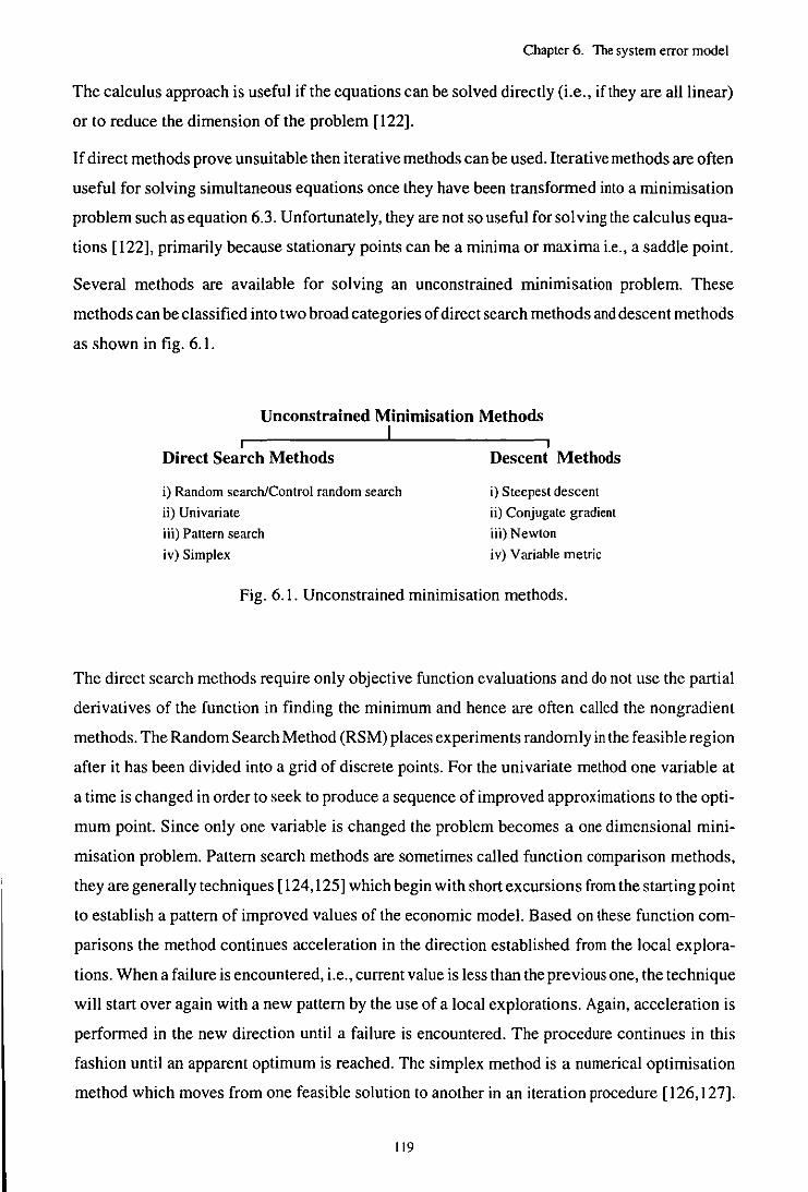
-------------
Chapter 6. The system error model
The calculus approach is useful if the equations can be solved directly (i.e., if they are all linear)
or to reduce the dimension of the problem [122].
If direct methods prove unsuitable then iterative methods can be used. Iterative methods are often
useful for solving simultaneous equations once they have been transformed into a minimisation
problem such as equation 6.3. Unfortunately, they are not so useful for sol ving the calculus equa
tions [122], primarily because stationary points can be a minima or maxima i.e., a saddle point.
Several methods are available for solving an unconstrained minimisation problem. These
methods can be classified into two broad categories of direct search methods and descent methods
as shown in fig. 6.1.
Unconstrained Minimisation Methods I
I Direct Search Methods
i) Random search/Control random search
ii) Univariate
iii) Pattern search
iv) Simplex
I Descent Methods
i) Steepest descent
ii) Conjugate gradient
iii) Newton
iv) Variable metric
Fig. 6.1. Unconstrained minimisation methods.
The direct search methods require only objective function evaluations and do not use the partial
derivatives of the function in finding the minimum and hence are often called the nongradient
methods. The Random Search Method (RSM) places experiments randomly in the feasible region
after it has been divided into a grid of discrete points. For the univariate method one variable at
a time is changed in order to seek to produce a sequence of improved approximations to the opti
mum point. Since only one variable is changed the problem becomes a one dimensional mini
misation problem. Pattern search methods are sometimes called function comparison methods,
they are generally techniques [124,125] which begin with short excursions from the starting point
to establish a pattern of improved values of the economic model. Based on these function com
parisons the method continues acceleration in the direction established from the local explora
tions. When a failure is encountered, i.e., current value is less than the previous one, the technique
will start over again with a new pattern by the use of a local explorations. Again, acceleration is
performed in the new direction until a failure is encountered. The procedure continues in this
fashion until an apparent optimum is reached. The simplex method is a numerical optimisation
method which moves from one feasible solution to another in an iteration procedure [126,127].
119
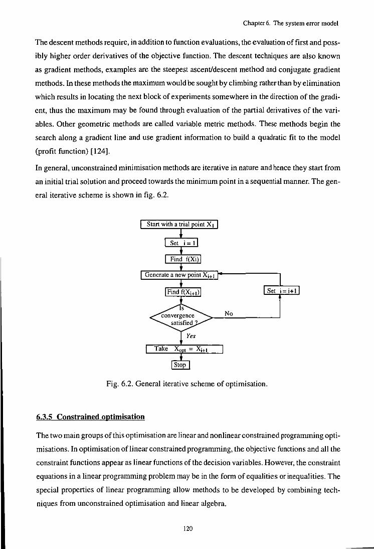
Chapter 6. The system error model
The descent methods require, in addition to function evaluations, the evaluation of first and poss
ibly higher order derivatives of the objective function. The descent techniques are also known
as gradient methods, examples are the steepest ascent/descent method and conjugate gradient
methods. In these methods the maximum would be sought by climbing rather than by elimination
which results in locating the next block of experiments somewhere in the direction of the gradi
ent, thus the maximum may be found through evaluation of the partial derivatives of the vari
ables. Other geometric methods are called variable metric methods. These methods begin the
search along a gradient line and use gradient infonnation to build a quadratic fit to the model
(profit function) [124].
In general, unconstrained minimisation methods are iterative in nature and hence they start from
an initial trial solution and proceed towards the minimum point in a sequential manner. The gen
eral iterative scheme is shown in fig. 6.2.
Generate a new point Xi+ I
No
Fig. 6.2. General iterative scheme of optimisation.
6.3.5 Constrained optimisation
The two main groups ofthis optimisation are linear and nonlinear constrained programming opti
misations. In optimisation of linear constrained programming, the objective functions and all the
constraint functions appear as linear functions of the decision variables. However, the constraint
equations in a linear programming problem may be in the fonn of equalities or inequalities. The
special properties of linear programming allow methods to be developed by combining tech
niques from unconstrained optimisation and linear algebra.
120
Chapter 6. The system error model
In non linear constrained optimisation the constraints imposed upon the variables imply a certain
nonlinear function. Methods for minimising this kind of functions can be divided broadly into
two classes, those which set up an equivalent unconstrained minimisation problem by adding a
penalty term to the objective function (i.e., barrier and penalty function methods), and those
which seek to generate a sequence of feasible descent steps which would involve linear approx
imation to the constraints [124,128,129].
6.3.6 Least souares best fit
Least squares fitting algorithms are optimisation routines to approximate to linear (such as, line
or plane) or non linear (such as, circles, spheres, cylinders and cones) functions by fitting features
to a set of data points. For the 2-D case of curve fitting, a set of n points as (XI, YI), .... , (xn, Yn)
are given and it is required to determine a function F(x) such that F(xj)"" Yio for i=1 , ... , n. The
method of least squares can be explained better by an example [120,130], if n pair of measure
ments, (XI, yd, .... , (xn, Yn) are required to be fitted to a straight line ofy = a + bx. The line should
be fitted through the points so that the sum of the squares of the distances of the points from the
straight line is to be minimum, the line is then in a unique position. The first task is to find esti
mated values of a and b such that the line gives a good fit to the data. At any point Xj the correspon
ding point on the line is given by a + bXj, so the difference between the observed value of y and
the predicted value can be given by
..... 6.4
The least squares estimates of a and b would be obtained by choosing the values which minimise
the sum of squares of these deviations (i.e., residuals). Thus the sum of the squared deviations
will be given by
n
S = I e2 I
..... 6.5 ;=1
n 2
S = I (y; - (a + b.)) ..... 6.6 ;=1
The equality is a function of the unknown parameters a and b, which can be minimised by calcu
lating partial derivatives ils/ila and ils/ilb, setting both these derivatives equal to zero, and solving
• the two simultaneous equations to obtain the least squares estimates, 11 and b, of a or b
121
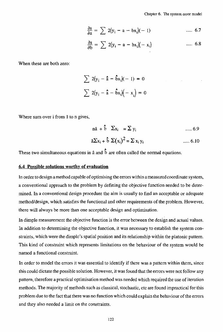
Chapter 6. The system error model
6.7
6.8
When these are both zero:
Where sum over i from I to n gives,
..... 6.9
..... 6.10
• These two simultaneous equations in it and b are often called the nonnal equations.
6.4 Possible solutions worthy of evaluation
In order to design a method capable of optirnising the errors within a measured coordinate system,
a conventional approach to the problem by defining the objective function needed to be deter
mined. In a conventional design procedure the aim is usually to find an acceptable or adequate
method/design, which satisfies the functional and other requirements of the problem. However,
there will always be more than one acceptable design and optirnisation.
In dimple measurement the objective function is the error between the design and actual values.
In addition to determining the objective function, it was necessary to establish the system con
straints, which were the dimple's spatial position and its relationship within the platonic pattern.
This kind of constraint which represents limitations on the behaviour of the system would be
named a functional constraint.
In order to model the errors it was essential to identify if there was a pattern within them, since
this could dictate the possible solution. However, it was found that the errors were not follow any
pattern, therefore a practical optimisation method was needed which required the use of iteration
methods. The majority of methods such as classical, stochastic, etc are found impractical for this
problem due to the fact thatthere was no function which could explain the behaviour of the errors
and they also needed a limit on the constraints.
122
Chapter 6. The system error model
One possible approach to this kind of problem was by optimising the data using CRSIRSM. One
of the main advantages of using this method is that no limits are required on the degree of con
straints within the system. The types of constraints were the size and the form or shape of the
pattern which all should be kept unchanged. It was anticipated that the use of RSM would mini
mise positions for the actual data [121,125,131] and although, the solution to the problem was
in three dimensions, a two dimensional solution was first developed for simplicity.
6.5 Proposed random search method for optimisation
As explained previously to classify an optimisation problem it is necessary to establish the nature
of the problem, for a golf ball the dimples could not be grouped in a linear or non linear form. It
was possible that the errors in a dimple pattern were generated through an imbiased machining
system with other possible shortcomings being in the design specification i.e., selecting the
wrong size dimple. The objective was to minimise positional errors. One of the most suitable
methods was to use a numerical optimisation i.e., RSMs sub group of the direct search methods.
These methods require only objective function evaluations and do not use the partial derivatives
of the function in finding the minimum which makes them most suitable for simple problems in
volving a relatively small number of variables. The use of a RSM for this work was envisaged
to be useful due to the nature of the problem i.e., not having prior knowledge of the behaviour
of the errors, therefore, there appeared to be no solution using any direct methods.
6.5.1 RSM experiments on the golf ball patterns
The procedure of the RSM algorithm is shown as a flow diagram in fig 6.3. The method has been
evaluated for a series of 2-D geometric pattern arrangements with arbitrary given points. For golf
ball dimples there are two sets of data, nominal and actual. In order to visualise the effect of opti
misation better, it was decided to assess graphically the pattern representation of dimples which
were created from the actual and nominal data. Therefore, the graphical representation of the
nominal pattern was assumed to be the target and that of the actual data was the objective to be
minimised. In order to implement the technique for this problem it was required to develop a con
straint function which was designed to be the sum of distances between these data points i.e., the
target length was made of the nominal values and the objective was made of the actual values.
In order to find optimisation positions for the target points each distance' e' between the trial and
the nominal point was stored for comparison to select the lowest value between them.
The dimple error minimisation will have a function of the sum of errors (i.e., objective function),
with n variables (dimple centre coordinates).
123
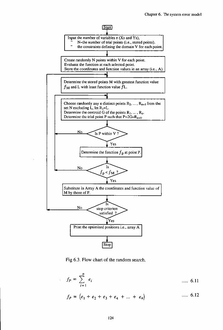
Chapter 6. The system error model
Input the number of variables n (Xs and Y s), .. N-the number of trial points (i.e., stored points).
the constraints defining the domain V for each point.
Create randomly N points within V for each point. Evaluate the function at each selected point. Store the coordinates and function values in an array (i.e., A).
Determine the stored points M with greatest function value fM and L with least function value fL.
Choose randomly any n distinct points R2, ... , RO+, from the set N excluding L, let R,=L. Determine the centroid G of the points R" ... , R,. Determine the trial point P such that P=2G-R,+,.
No
Determine the function f p at point P.
No
Substitute in Array A the coordinates and function value of M by those of P.
No
Print the optimised positions i.e., array A
Fig 6.3. Flow chart of the random search.
n
JP = I ej i= I
Jp = (el + e2 + e3 + e4 + ... + en)
124
..... 6.11
..... 6.12
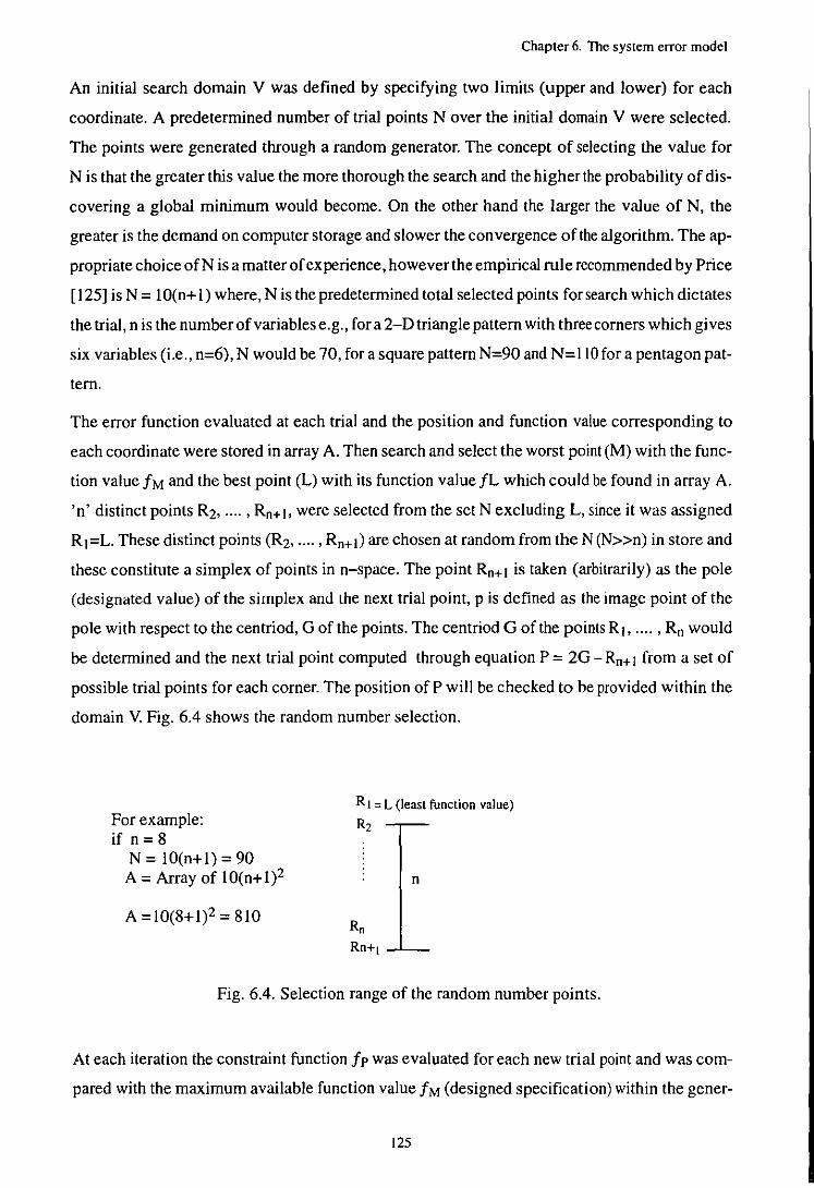
Chapter 6. The system error model
An initial search domain V was defined by specifying two limits (upper and lower) for each
coordinate. A predetermined number of trial points N over the initial domain V were selected.
The points were generated through a random generator. The concept of selecting the value for
N is that the greater this value the more thorough the search and the higher the probability of dis
covering a global minimum would become. On the other hand the larger the value of N, the
greater is the demand on computer storage and slower the convergence of the algorithm. The ap
propriate choice ofN is a matter of experience, howeverthe empirical rule recommended by Price
[125] is N = lO(n+ 1) where, N is the predetermined total selected points for search which dictates
the trial, n is the number of variables e.g., for a 2-D triangle pattern with three corners which gives
six variables (i.e., n=6), N would be 70, for a square pattern N=90 and N=11O for a pentagon pat-
tern.
The error function evaluated at each trial and the position and function value corresponding to
each coordinate were stored in array A. Then search and select the worst point (M) with the func
tion value fM and the best point (L) with its function value fL which could be found in array A.
'n' distinct points R2, .... , Rn+l, were selected from the set N excluding L, since it was assigned
RJ=L. These distinct points (R2, .... , Rn+J) are chosen at random from the N (N)>n) in store and
these constitute a simplex of points in n-space. The point Rn+t is taken (arbitrarily) as the pole
(designated value) of the simplex and the next trial point, p is defined as the image point of the
pole with respect to the centriod, 0 of the points. The centriod G of the points Rh .... , Rn would
be determined and the next trial point computed through equation P = 20 - Rn+ J from a set of
possible trial points for each corner. The position of P will be checked to be provided within the
domain V. Fig. 6.4 shows the random number selection.
For example: if n = 8
N = lO(n+l) = 90 A = Array of lO(n+l)2
A =10(8+1)2 = 810
RI = L (least function value)
R2
n
Fig. 6.4. Selection range of the random number points.
At each iteration the constraint function fp was evaluated for each new trial point and was com
pared with the maximum available function value fM (designed specification) within the gener-
125
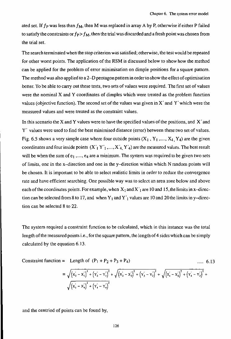
Chapter 6. The system error model
ated set. If fp was less than fM, then M was replaced in array A by P, otherwise if either P failed
to satisfy the constraints or fp> fM, then the trial was discarded and a fresh point was chosen from
the trial set.
The search tenninated when the stop criterion was satisfied; otherwise, the test would be repeated
for other worst points. The application of the RSM is discussed below to show how the method
can be applied for the problem of error minimisation on dimple positions for a square pattern.
The method was also applied to a 2-D pentagon pattern in order to show the effect of optimisation
better. To be able to carry out these tests, two sets of values were required. The first set of values
were the nominal X and Y coordinates of dimples which were treated as the problem function
values (objective function). The second set of the values was given in X' and Y' which were the
measured values and were treated as the constraint values.
In this scenario the X and Y values were to have the specified values of the positions, and X' and
Y' values were used to find the best minimised distance (error) between these two set of values.
Fig. 6.5 shows a very simple case where four outside points (X I , Y I ,.,," X4, Y 4) are the given
coordinates and four inside points (X'I Y 'I, .. ", X '4, Y'4) are the measured values. The best result
will be when the sum of el , .... , e4 are a minimum. The system was required to be given two sets
of limits, one in the x-direction and one in the y-direction within which N random points will
be chosen. It is important to be able to select realistic limits in order to reduce the convergence
rate and have efficient searching. One possible way was to select an area zone below and above
each of the coordinates points. For example, when XI andX' I are iO and 15, the limits in x-direc
tion can be selected from 8 to 17, and when Y I and Y' 1 values are 10 and 20 the limits in y-direc
tion can be selected 8 to 22.
The system required a constraint function to be calculated, which in this instance was the total
length of the measured points i.e., for the square pattern, the length of 4 sides which can be simply
calculated by the equation 6.13,
Constraint function = Length of (PI + P2 + P3 + P 4) "". 6.13
= j(x; - x;)' + h -v;)' + j(x; -x;)' + (v; - v;)' + j(x; - x;)' + (y; - v;)' +
j(x; -x;)' + (y; - v;)'
and the centriod of points can be found by,
126
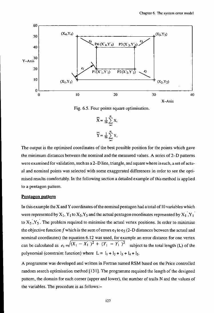
Chapter 6. The system error model
60,----------------------------------------------------,
so
40
30 Y-Axis
20
ID ~
~ P4 (X '4. Y '4)
~ PI(X'I,Y'I)
P3(X'3.Y · ) y
P2(X·2.Y ·2 'Z
OL-------------------------------------------------~ o ID 20
Fig. 6.5. Four points square optimisation.
_ m
X=.l ""X mL ' j,.\
30 40
X-Axis
The output is the optimised coordinates of the best possible position for the points which gave
the minimum distances between the nominal and the measured values. A series of 2-D patterns
were examined for validation, such as a 2-D line, triangle, and square where in each, a set of actu
al and nominal points was selected with some exaggerated differences in order to see the opti
mised results comfortably. In the following section a detailed example of this method is applied
to a pentagon pattern.
PentaJ:on pattern
In this example the X and Y coordinates of the nominal pentagon had a total of 10 variables which
were represented by X I, Y I to Xs, Y s and the actual pentagon coordinates represented by X I ',Y I
to Xs ,Y s . The problem required to minimise the actual vertex positions. In order to minimise
the objective function f which is the sum of errors el to es (2-D distances between the actual and
nominal coordinates) the equation 6.12 was used, for example an error distance for one vertex I . 2 . 2
can be calculated as el =v (XI - Xl) + (YI - YI) subject to the totallength (L) of the
polynomial (constraint function) where L = I1 + 12 + 13 + 14 + 15,
A programme was developed and written in Fortran named RSM based on the Price controlled
random search optimisation method [131]. The programme required the length of the designed
pattern, the domain for each corner (upper and lower), the number of trails N and the values of
the variables. The procedure is as follows:-
127
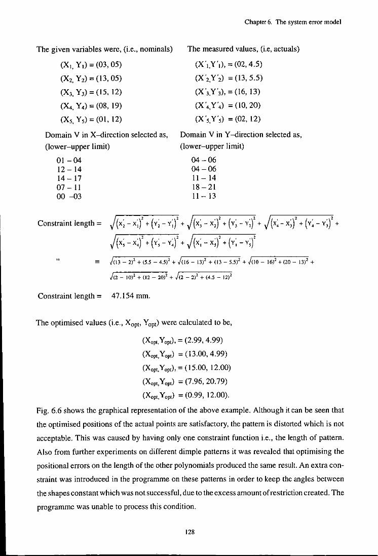
Chapter 6. The system error model
The given variables were, (i.e., nominals) The measured values, (i.e, actuals)
(X, Y,) = (03, 05)
(X2, Y 2) = (13, 05)
(X3 Y 3) = (IS, 12)
(X4 Y4) = (08, 19)
(X5, Y 5) = (01, 12)
(X·,.Y',), = (02, 4.5)
(X'2,Y'2) = (13, 5.5)
(X'3.Y'3), = (16,13)
(X '4 Y'4) = (10, 20)
(X '5,Y'5) = (02, 12)
Domain V in X-direction selected as,
(lower-upper limit)
Domain V in Y -direction selected as,
(lower-upper limit)
01-04 04-06 12 - 14 04-06 14 - 17 11 - 14 07 - 11 18 - 21 00 -03 11 - 13
Constraint length = j(x; -x;)' + (v; - y;)' + j(x; - x;)' + h - y;)' + j(x; -x;)' + (y; - y;)' +
j(x; -x;)' + h - y;)' + j(x; _ x;)' + (y; _ y;)'
" = /(13 - 2)' + (5.5 - 4.5)' + /(16 - (3)' + (13 - 5.5)' + /(10 - (6)2 + (20 - 13)' +
/(2 - 10)' + (12 - 20)' + /(2 - 2)' + (4.5 - 12)'
Constraint length = 47.154 mm.
The optimised values (i.e., Xopt> Yopt) were calculated to be,
(Xopt.Yopt), = (2.99, 4.99)
(Xopt,Yopt) = (13.00, 4.99)
(Xopt.Yopt), = (15.00, 12.00)
(Xopt,Yopt) = (7.96, 20.79)
(Xopt.Yopt) = (0.99, 12.00).
Fig. 6.6 shows the graphical representation of the above example. Although it can be seen that
the optimised positions of the actual points are satisfactory, the pattern is distorted which is not
acceptable. This was caused by having only one constraint function i.e., the length of pattern.
Also from further experiments on different dimple patterns it was revealed that optimising the
positional errors on the length of the other polynomials produced the same result. An extra con
straint was introduced in the programme on these patterns in order to keep the angles between
the shapes constant which was not successful, due to the excess amount of restriction created. The
programme was unable to process this condition.
128
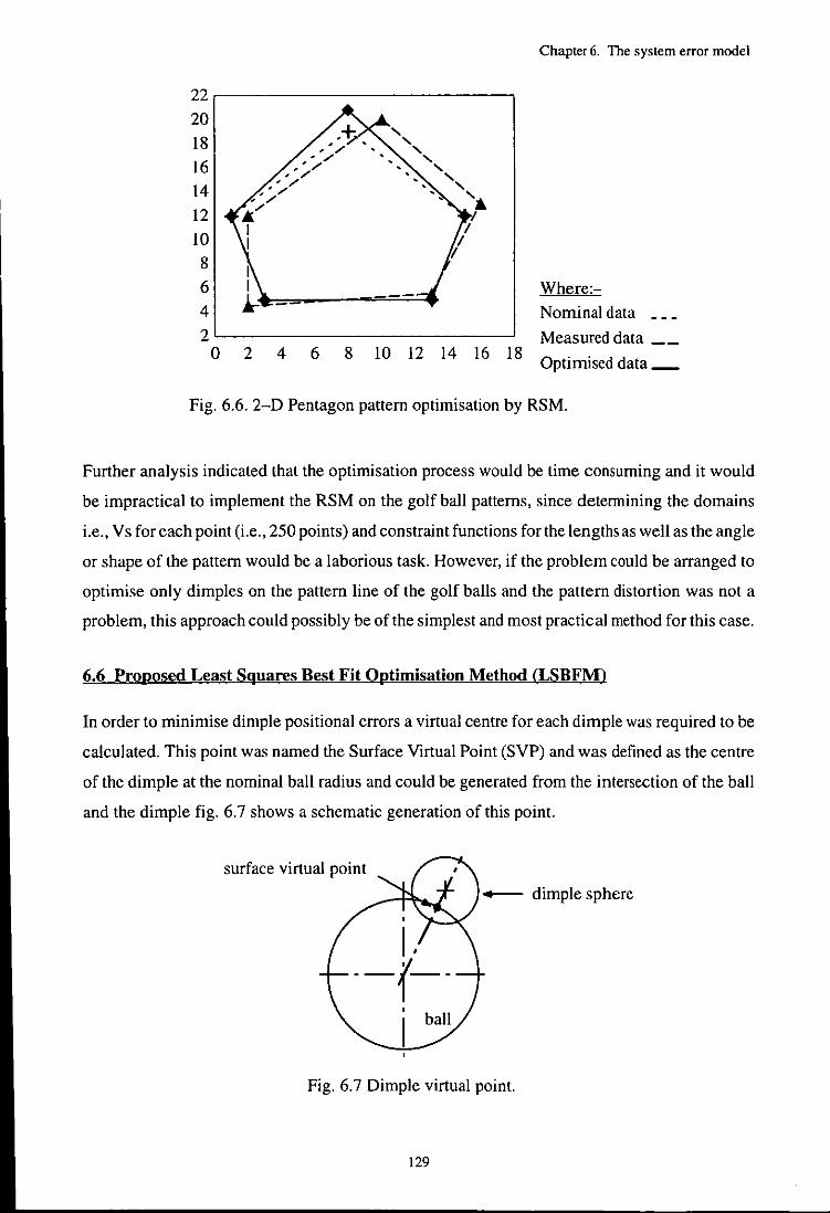
Chapter 6. The system error model
22
20 , 18 , , 16
, , , 14
, ' ..
12 1
10 /
/
8 'I
6 --- Where:-4 Nominal data 2 Measured data __
0 2 4 6 8 10 12 14 16 18 Optimised data _
Fig. 6.6. 2-D Pentagon pattern optimisation by RSM.
Further analysis indicated that the optimisation process would be time consuming and it would
be impractical to implement the RSM on the golf ball patterns, since detennining the domains
i.e., Vs for each point (i.e., 250 points) and constraint functions forthe lengths as well as the angle
or shape of the pattern would be a laborious task. However, if the problem could be arranged to
optimise only dimples on the pattern line of the golf balls and the pattern distortion was not a
problem, this approach could possibly be of the simplest and most practical method for this case.
6.6 Proposed Least Squares Best Fit Optimisation Method (LSBFM)
In order to minimise dimple positional errors a virtual centre for each dimple was required to be
calculated. This point was named the Surface Virtual Point (SVP) and was defined as the centre
of the dimple at the nominal ball radius and could be generated from the intersection of the ball
and the dimple fig. 6.7 shows a schematic generation of this point.
surface virtual point
I . --{--
ball
- dimple sphere
Fig. 6.7 Dimple virtual point.
129
Chapter 6. The system error model
The importance of these points was appreciated when the nominal and actual data needed to be
compared in order to establish possible production variances whlch may then improve the pro
duction of the part by finding the source of variation.
The error at each virtual centre should be calculated individually and then compared to that of
other centres in order to satisfy a restricted pattern. A survey of literature has revealed no analyti
cal method for assessing this type of 3-D error optimisation.
In essence, the proposed optimisation method finds the best point positions for the errors by use
of a number of trials on the objective function in order to give critical values or a set of minimum
values subject to certain constraints on the control variables. 3-D optimisation was used for each
trial, with the calculation of the objective function for all the points in three axes.
A comparison was made between the nominal designed values to those of the actual data which
were obtained through measurement on the CMM. The required limits on the data were selected
no wider than the distance between two dimple thus, the relationships between the dimples was
ensured.
The software employed for this section of the project was developed and written in C and its flow
diagram can be found in fig. 6.8. The programme requires a tolerance zone which depends on
the size type of dimples used on the ball and permits the points to be assessed in three axes for
both negative and positive directions. One of the outputs of the programme was the optimised
positions of the actual points and some others were the length of the objective function, and the
value of residuals. Sequentially a small value in different directions was added or subtracted to
the coordinates and the objective function evaluated. The objective function was then recorded
and compared in order to select the objective function with the minimum value which would refer
to the best position of the data. The method of optimisation was arranged in cartesian form, how
ever, the polar approach would have a similar concept and is explained later.
6.6.1 Cartesian approach
The first step is to create an objective function, an example of which can be the location of the
dimples on the surface of a ball. The dimples are machined in relation to the ball center as well
as to a pattern. The machining of the dimples requires positioning in 5 axes, which results in some
error between the specified and actual positions. These positional errors generally do not occur
in a controlled manner. Once the positional errors are established a method is required to mini
mise the errors in a controlled process.
The objective function for this problem was based on the distance between the nominal positions
and the actual positions. The objective function needed to be minimised which required the cal-
130
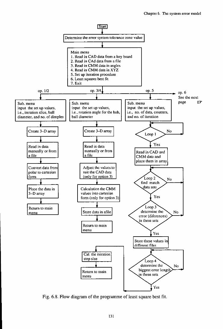
op. 112
Sub. menu input the set up values, Le., iteration slice, ball diameter, and no. of dimples
Read in data manually or from a file
Conven data from polar to cartesian form
Place the data in 3-D array
Return to main menu
Chapter 6. The system error model
Determine the error syetem tolerance zone value
Main menu I. Read in CAD data from a key board 2. Read in CAd data from a file 3. Read in CMM data in angles 4. Read in CMM data in XYZ 5. Set up iteration procedure 6. Least squares best fit 7. Exit
Sub. menu input the set up values, i.e., rotation angle for the hob, ball diameter
Read in data manually or from a file
Adjust the values to suit the CAD data
Calculation the CMM values into cartesian form (only for option 3)
Return to main menu
Return to main menu
op.5
Sub. menu input the set up values, i.c., no. of data, counters, and no. of iteration
No
Read in CAD and CMM data and place them in array
No
Loop 3 determine the
error (diferences) in these sets
Yes
Store these values in different files
op.6 See the next page 117
No
No
Fig. 6.8. Flow diagram of the programme of least square best fit.
131
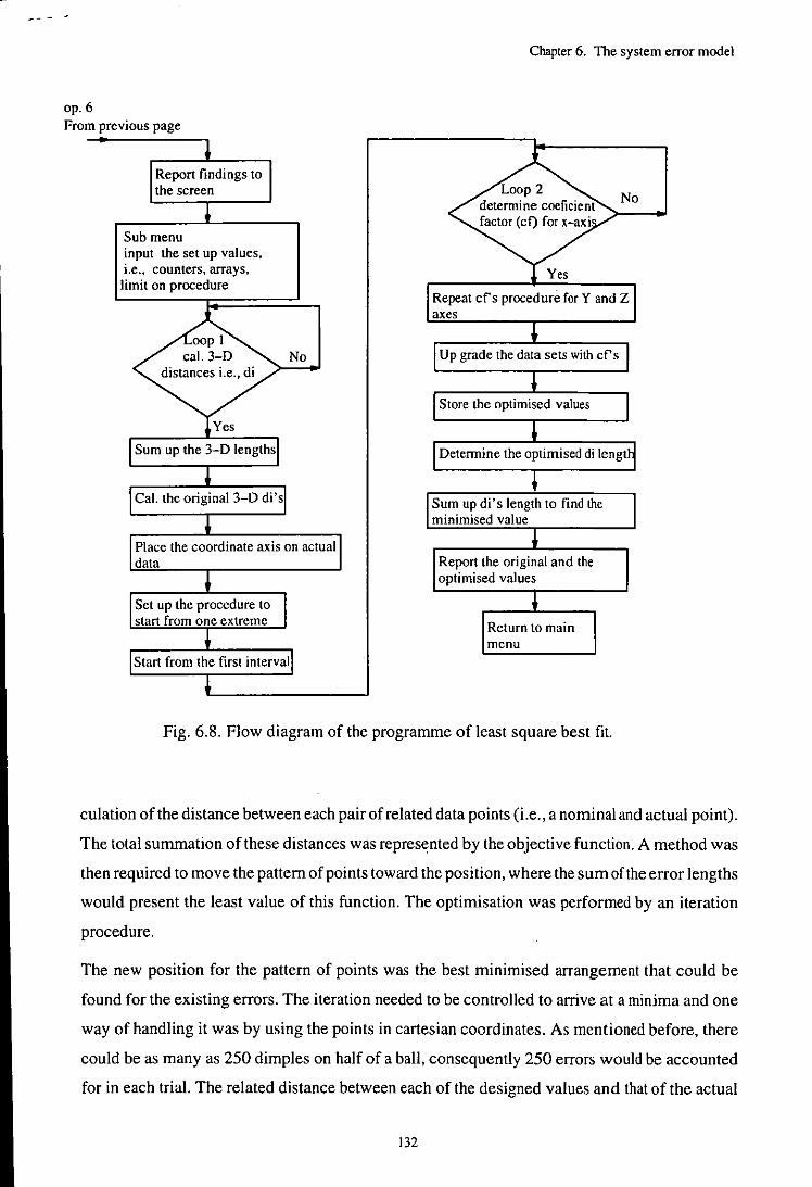
op.6 From previous page
Report findings to the screen
Sub menu input the set up values, i.e., counters, arrays, limit on procedure
No
Chapter 6. The system error model
No
Repeat efs procedure for Y and Z axes
Upgrade the data sets with ef s
Store the optimised values
Determine the optimised di lengt
Sum up di' s length to find the minimised value
Report the original and the optimised values
Return to main menu
Fig. 6.8. Flow diagram of the programme of least square best fit.
culation of the distance between each pair of related data points (i.e., a nominal and actual point).
The total summation of these distances was represented by the objective function. A method was
then required to move the pattern of points toward the position, where the sum of the error lengths
would present the least value of this function. The optimisation was performed by an iteration
procedure.
The new position for the pattern of points was the best minimised arrangement that could be
found for the existing errors. The iteration needed to be controlled to arrive at a minima and one
way of handling it was by using the points in cartesian coordinates. As mentioned before, there
could be as many as 250 dimples on half of a ball, consequently 250 errors would be accounted
for in each trial. The related distance between each of the designed values and that of the actual
132

Chapter 6. The system error model
value was named d; with i designating the number of dimple. The use of this method would not
restrict the amount of data, and the objective equation can be written as:-
;=n=250 E = I (d;)2 ..... 6.14
i=l
;=n=250 E = I [Xnj - Xaj ± (dX)j2 + [Ynj - Yaj ± (dYW + [Zn; - Zaj ± (dZW
j=l ..... 6.15
Where E is the objective function, dX, d Y, and e:,Z are the iteration step sizes, and d; is the error
between each data pair set.
One of the important factors in this method was how the iteration could be controlled. The best
position for each piece of data was when its positional error was zero and ideally that was achiev
able when all the nominal points and the actual points could be coincidentally located. To initiate
the iteration a starting point was required, logically in such an iteration a starting point could be
a point with the worst global characteristic (i.e., a pair of data points which gave the maximum
separation length). The worst case of the error length was the maximum calculated error length
which could be found between the axes of a data set (i.e., IXmaxl, IYmaxl or IZmaxl), however,
a simple solution would be to take the largest absolute length value which could be found within
the set, i.e., I(X, - X,) + (Y, - Y,) + (Z, - Z.)I .
6.6.2 Calculation of the domains
The values of ± Xmax, ± Ymax and ± Zmax are the extremes which will be selected for the iter
ation domains. The 3-D error lengths can be determined in relation to the ball centre, by calculat
ing the distance between the actual and nominal data. In order for the optimisation to proceed the
largest possible error between the data sets i.e., the largest 3-D error between the data sets was
selected and the domains for three axes were set, based on this value. This would cover any error
between the data sets in any plane.
Once the domains are determined an imaginary box was created and placed on the actual data.
A local coordinate axis was placed at the centre of the box with the domains at negative and posi
tive sides of the axes, where each axis represented error in that direction with indexed intervals,
e.g., X;nt.. Fig. 6.9 schematically shows this arrangement.
133
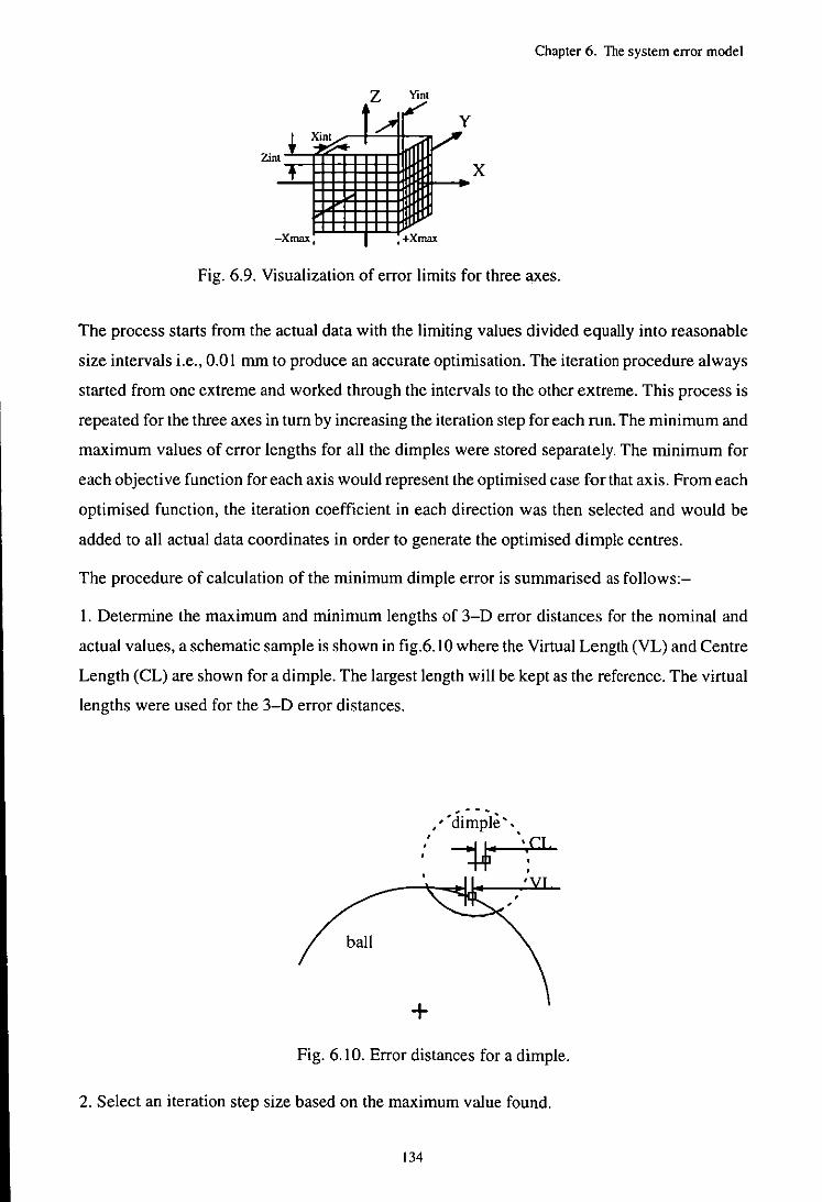
Chapter 6. The system error model
Z Yinl
Zinl x
-Xmax, ,+Xmax
Fig. 6.9. Visualization of error limits for three axes.
The process starts from the actual data with the limiting values divided equally into reasonable
size intervals i.e., 0.0 I mm to produce an accurate optimisation. The iteration procedure always
started from one extreme and worked through the intervals to the other extreme. This process is
repeated for the three axes in turn by increasing the iteration step for each run. The minimum and
maximum values of error lengths for all the dimples were stored separately. The minimum for
each objective function for each axis would represent the optimised case for that axis. From each
optimised function, the iteration coefficient in each direction was then selected and would be
added to all actual data coordinates in order to generate the optimised dimple centres.
The procedure of calculation of the minimum dimple error is summarised as follows:-
I. Determine the maximum and minimum lengths of 3-D error distances for the nominal and
actual values, a schematic sample is shown in fig.6.1O where the Virtual Length (VL) and Centre
Length (CL) are shown for a dimple. The largest length will be kept as the reference. The virtual
lengths were used for the 3-D error distances.
ball
+ Fig. 6.10. Error distances for a dimple.
2. Select an iteration step size based on the maximum value found.
134

Chapler 6. The system error model
3. Divide the limits into equal intervals for both positive and negative directions similar to that
in fig. 6.9.
4. Run the process for each axis.
5. Calculate the squared length of errors for each pair set.
6. Repeat step 5 for all the dimple pairs.
7. Repeat step 5 for all combinations of the intervals.
8. Sum the squared error lengths for each iteration.
9. Compare the calculated error lengths for each iteration to find the minimum for three axes.
10. Determine the correction factor for each axis from step 9.
11. Find the 3-D optimum location in X, Y, and Z values from the minimum cases.
12. Place the original error axes found from step 11 in the new error axes arrangement for one
more investigation.
13. Repeat step 3 to step 9 to possibly arrive at a better accuracy around the optimum point.
14. Determine the new locations (optimised) by adding/subtracting the correction factor to the
actual data locations.
15. Evaluate the optimised positions by graphical representation of the actual and optimised data
to that of the specified values.
A series of tests were carried out on cubic and icosddh 432 hobs 10 support this theory. The
dimples on the hobs were measured three times to ensure consistency of the results. Each of the
measured data was processed by the proposed optimisation method and new values were calcu
lated. In order to represent the results graphically on the Unigraphics CAD system it was necess
ary to distinguish this data by using different colours for data sets, e.g. the nominal data was repre
sented with colour red. A sampled set of the optimised results for the cubic and icosddh 432 hobs
are listed in appendix A.
In order to study the results an example from the icosddh 432 sets (appendix A) is selected and
explained in detail in fig 6.11;-
135
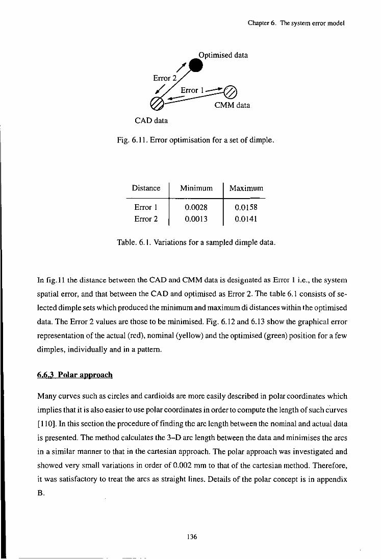
Chapter 6. The system error model
Optimised data
CMMdata
CAD data
Fig. 6.11. Error optimisation for a set of dimple.
Distance
Error I
Error 2
Minimum
0.0028
0.0013
Maximum
0.0158
0.0141
Table. 6.1. Variations for a sampled dimple data.
In fig.11 the distance between the CAD and CMM data is designated as Error I i.e., the system
spatial error, and that between the CAD and optimised as Error 2. The table 6.1 consists of se
lected dimple sets which produced the minimum and maximum di distances within the optimised
data. The Error 2 values are those to be minimised. Fig. 6.12 and 6.13 show the graphical error
representation of the actual (red), nominal (yellow) and the optimised (green) position for a few
dimples, individually and in a pattern.
6.6.3 Polar approach
Many curves such as circles and cardioids are more easily described in polar coordinates which
implies that it is also easier to use polar coordinates in order to compute the length of such curves
[110]. In this section the procedure of finding the arc length between the nominal and actual data
is presented. The method calculates the 3-D arc length between the data and minimises the arcs
in a similar manner to that in the cartesian approach. The polar approach was investigated and
showed very small variations in order of 0.002 mm to that of the cartesian method. Therefore,
it was satisfactory to treat the arcs as straight lines. Details of the polar concept is in appendix
B.
136
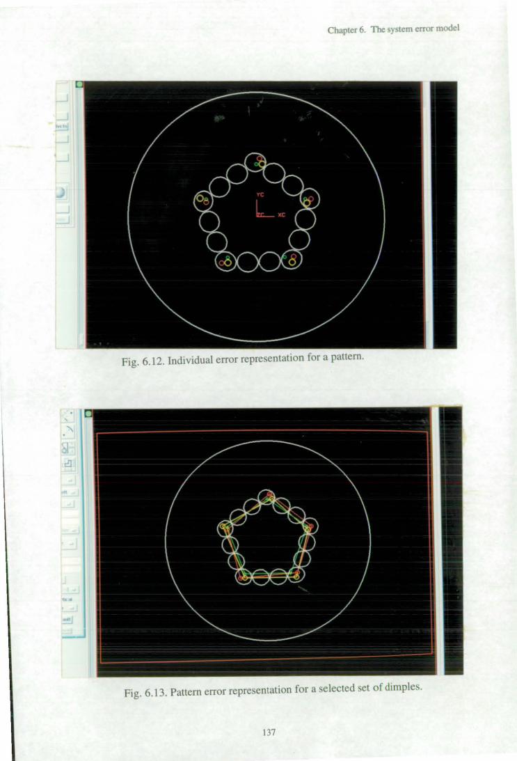
Chapter 6. The system error model
Fig. 6.12. Individual error representation for a pattern.
Fig. 6.13. Pattern error representation for a selected set of dimples.
137
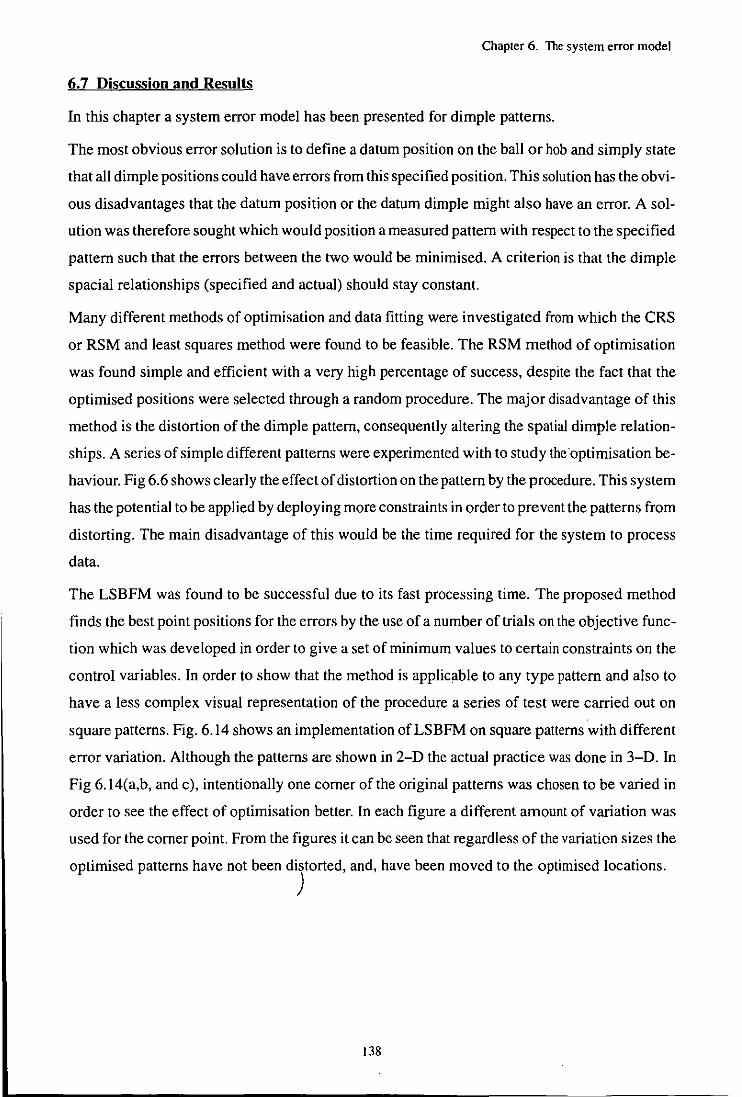
Chapter 6. The system error model
6.7 Discussion and Results
In this chapter a system error model has been presented for dimple patterns.
The most obvious error solution is to define a datum position on the ball or hob and simply state
that all dimple positions could have errors from this specified position. This solution has the obvi
ous disadvantages that the datum position or the datum dimple might also have an error. A sol
ution was therefore sought which would position a measured pattern with respect to the specified
pattern such that the errors between the two would be minimised. A criterion is that the dimple
spacial relationships (specified and actual) should stay constant.
Many different methods of optimisation and data fitting were investigated from which the CRS
or RSM and least squares method were found to be feasible. The RSM rnelhod of optimisation
was found simple and efficient with a very high percentage of success, despite the fact that the
optimised positions were selected through a random procedure. The major disadvantage of this
method is the distortion of the dimple pattern, consequently altering the spatial dimple relation
ships. A series of simple different patterns were experimented with to study the·optimisation be
haviour. Fig 6.6 shows clearly the effect of distortion on the pattern by the procedure. This system
has the potential to be applied by deploying more constraints in order to prevent the patterns from
distorting. The main disadvantage of this would be the time required for the system to process
data.
The LSBFM was found to be successful due to its fast processing time. The proposed method
finds the best point positions for the errors by the use of a number of trials on the objective func
tion which was developed in order to give a set of minimum values to certain constraints on the
control variables. In order to show that the method is applicable to any type pattern and also to
have a less complex visual representation of the procedure a series of test were carried out on
square patterns. Fig. 6.14 shows an implementation of LSBFM on square patterns with different
error variation. Although the patterns are shown in 2-D the actual practice was done in 3-D. In
Fig 6.14(a,b, and c), intentionally one corner of the original patterns was chosen to be varied in
order to see the effect of optimisation better. In each figure a different amount of variation was
used for the corner point. From the figures it can be seen that regardless of the variation sizes the
optimised patterns have not been distorted, and, have been moved to the optimised locations. )
138
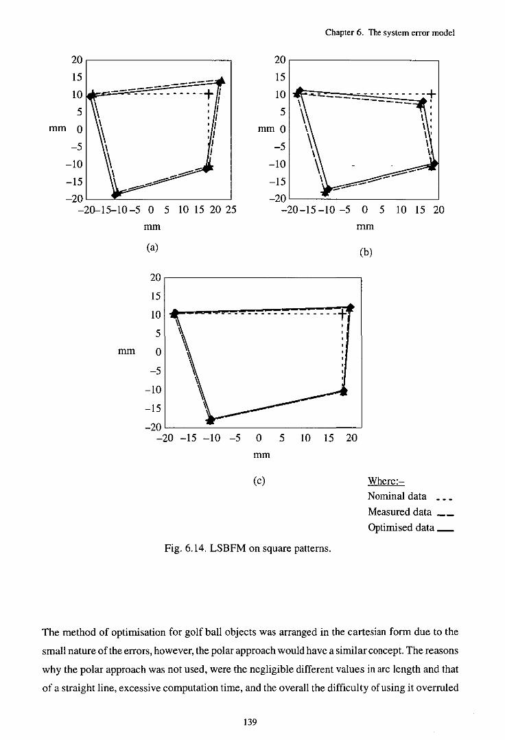
20
15
10
5
mm 0
-5
-10
-15
, I , I , I , I : I I I
Chapter 6. The system error model
20,-----------------~
15
10 ~~~~~~~ 5
mm 0
-5
-10
-15 -~-:::::--
:::;--
\ : \ ' \ ' \ \
-20L-~~------------~ -20L---~------------~ -20-15-10-5 0 5 10 15 20 25 -20-15 -10 -5 0 5 10 15 20
mm
mm
(a)
20
15
10 ,-5 ~
0 ~ ~
-5 ,
~ -10 \ -15
-20 ...
-20 -15 -10
mm
---- ----- - ----- ---f
-5 0 5 10 15 20
mm
(c)
(b)
Where:-
Nominal data
Measured data __
Optimised data _
Fig. 6.14. LSBFM on square patterns.
The method of optimisation for golf ball objects was arranged in the cartesian form due to the
small nature of the errors, however, the polar approach would have a similar concept. The reasons
why the polar approach was not used, were the negligible different values in arc length and that
of a straight line, excessive computation time, and the overall the difficulty of using it overruled
139

Chapter 6. The system error model
applying it, a simple calculation of the error with the use of polar and cartesian method is in ap
pendix B in order to appreciate the amount of variation for an arc and straight line.
One of the main difficulties regarding the positional error for dimples was specifying the possible
error which could be generated by the CMM. The designed (dimple locations) was presented by
8 and <I> angles from a reference (datum) dimple. In order to address the dimples it was necessary
to align the reference dimple to the CMM axes. In the case of the icosddh 432 hob specification
the reference dimple was given by a type A dimple, dimple number 16 positioned at 8=0.000° and
<1>=22.762° (degrees), however when this dimple was measured on the actual hob by the CMM,
8 was found to be 16.728° and <1>= 0.241 0. The measured data was adjusted to these values for
the error modelling. One of the problem or inaccuracy of the system is the datum dimple might
be in error which in this case referring all other dimples to the datum dimple could generate a
situation where the correct dimples will be assumed wrong.
140
7.0 Introduction
Chapter 7. Interfacing CAD and CMM
CHAPTER 7
INTERFACING CAD AND CMM
CAD and CMMs have been available for some time, but until recently they have been largely used
individually. In recent years the practicalities of integrating a CAD system with a CMM have
changed dramatically because of the savings which can be made by using them concurrently in
manufacturing and inspection industries. In order to allow such integration to happen component
geometry information needs to be transferred from the CAD system to a CMM or vice versa by
data files developed through a standard protocol. There is a need for an inspection planner to take
the designed model consisting of specification of the part geometry, dimensioning and toleranc
ing information to produce an automatic inspection plan and programmes with detailed instruc
tions. One of the practical applications of CAD and CMM integration is seen in mould design,
where the CAD system is linked to one or more CNC machining centres [55,132).
With the rapid development of CMMs and associated softwares data can be more quickly and
accurately collected by using various probing systems to sense a surface or feature, and used to
create CAD drawings for documentation, or a part programme for an appropriate machine tool.
One prime use of CMM data collection is to evaluate the part dimensions against the specified
values in order to establish errors with the further enhancement of showing the graphical repre
sentation of their existence. There are many industrial environments where the CAD and CMM
link [39,40,55,75,85,101,132,133,134] to give benefits. Reverse engineering where the CAD
model is created by using data collected by a CMM is also a significant application area particu
larly for sculptured parts which may have been hand crafted.
In the following section the term CAD is used for a system which is accompanied with an inspec
tion post processor module as one unit.
In order to achieve an effective and useful integration between an inspection module of a CAD
and CMM the following needs to be considered [40]:
i) Generation of inspection programs.
ii) Creation of a data format for transfer of inspection information to CMM.
iii) Compatible CMM software which can interpret CAD generated files.
iv) Use of a data format for transfer of inspection results back to CAD.
Conceptually, for a CAD directed CMM there are three main areas to be considered. The first area
concerns with the creation of an inspection file in the CAD inspection module which uses the
141
Chapter 7. Interfacing CAD and CMM
design data. The second area deals with the definition of all features to be used in the process,
including all datuIns and attributes. The final area takes responsibility of determining the inspec
tion paths for each feature which can usually be previewed graphically on a CAD system.
In this work the integration is between a Tesa CMM and the Vnigraphics (VG) 3-D CAD
modeller. Ideally automatic transfer of a set of data which represents dimples on a golf ball would
be through a local network. The data was arranged in the form of X, Y,Z centre coordinates of
the dimples accompanied by the dimple diameter. Due to unavailability of the software at the time
in orderto perform an automatic transfer of data between the two systems, the work was manually
carried out by inputting data into the CAD system. The work planned to use the VG spreadsheet
application named VGlXess with a user function to process the model (see recommendation for
future work). The VGlXess allows creation and update of a VG family of parts and these tables
can also be imported from other PC spreadsheet applications. VG expressions are converted to
formulas in VGlXess, so users quickly see changes to the model when different values are used.
In order to support and appreciate the inspection procedure and also to visualise the order of preci
sion a graphical comparison was generated between the actual and nominal data (section 7.4).
7.1 Review of CAD and CMM integration
The issue of CAD and CMM interfacing has been the subject of research for a number of years
in order to improve the speed of inspection and overcome the difficulty of measuring complex
parts. This has been influenced mainly by the increasing roles of CMM's as a fast, flexible, and
accurate measuring tool in a high demand automated production area, however the majority of
work has been for prismatic parts. Cowling and Mullineux [39], McCarthy and Genest [55],
Farmer and Smith [75], Powaser [133] and others have studied the importance of inspection pro
cess requirements. They agree that for an efficient integration between the two systems a standard
file format is crucial.
The role of CAD and CMM integration has been one of the main objectives of the National Re
search Council of Canada (NRCC) [3] in order to develop an automated machining cell. In their
system a closed loop inspection system inspects production from the cell and communicates the
results to the cell controller. Through this integration the measured data from the CMM is trans
ferred to the CAD computer for analysis.
As mentioned previously Takeuchi et al. [4] used a vision based system to develop an automated
inspection environment. They also used a solid modelling CAD/CAM system named P-CAPS
to generate the CMM measuring path for the manufactured parts. From the CAD data a set of
measuring points on the workpiece were selected and each feature measured automatically in turn
142
Chapter 7. Interfacing CAD and CMM
as they were constructed by the CAD system. The system is useful only for mechanical parts
which are composed of a combination of primitives.
In a Computer Aided Inspection (CAI) system Pahk et al. [76] developed an interactive and inte
grated inspection system for moulds having sculptured surfaces with some basic features such
as holes and slots .. The CAD system contained the model from which features were selected man
ually for inspection and inspection planning was arranged for each feature. Osbaldiston et al.
[135] attempted to combine CAD and CAI in an interactive programming environment with the
target criteria to produce a system capable of extracting geometric information for prismatic parts
from any CAD system supporting IGES in order to generate inspection part programmes. In their
system the data was used to form the basis of an interactive programming environment capable
of generating inspection part programmes conforming to the DMIS. The methodology of their
work was to extract 2-D geometric data from an IGES file and recreate the drawing as accurately
as possible by the Graphical Kernel System (GKS) on the chosen output device. The DMIS part
programme for this file was then generated by instructing the system with the type of commands
required at any particular points in the part programme i.e., an accompanying piece of code to
specify the feature for example cir. for a circle.
Lu et al. [100] researched into establishing an AI inspection path planning system to avoid re
peated routes and to provide the best movement path between the components. Their attention
was based on optimal path planning for the whole measurement task which included finding the
shortest inspection path for multiple components. The AI path planning system required input
of component information which could be read into the data processing unit through CAD fIles,
from a vision system data file or input manually.
It is apparent that automated inspection planning is an extremely complex subject, and further
research is needed to develop this area. Unfortunately, all the interfaces which have been devel
oped between the CMM and CAD to date have been for particular CAD systems. Since there is
no universal translator for this link, it was seen necessary to arrange a link between the UG CAD
and the Tesa CMM for this work.
7.2 Generation of CAD datalReverse engineering of parts
The use of computers to create product designs is primarily a geometry based activity which is
organised to manipulate coordinate data points into lines, planes, and other geometric shapes.
Free formed and complex surfaces require considerable data to represent them, and generation
of this data is not an easy task. If the component has been designed during a crafting process so
that it is the design specification, the collection of data of part requires intelligent analysis, es-
143
Chapter 7. Interfacing CAD and CMM
timation of features and the density of points to be sampled to give good surface representation.
It is useful wherever possible to build a feature with a known set of properties and then transfer
it to the CAD system. In order to identify and provide a suitable set of data for the CAD system
in this work it was necessary to appreciate the systems requirements and the information required
for the integration and modelling.
CMMs have a variety of methods for generating the information necessary to create an inspection
procedure, two such methods are manually inputting information, or using the system routines
to measure a feature. A stream of data points which is generated on the CMM can be grouped
and transferred to the CAD database and can be used to generate a graphical representation of
the object. In order to manipulate prismatic part data into geometry shapes a feature identification
code is needed to accompany each group of data e.g., if the data is taken from a cylinder a code
which identifies the cylinder should accompany the data. In a reverse situation i.e., linking CAD
to a CMM, an additional element such as a probe path for inspection of the designed feature is
necessary to be added to the transferring data file. In the case of free form geometric shapes other
arrangements need considering, e.g., selection of one or more reference points to which the group
of data can be referred. When a CMM inspection is to be conducted by a CAD system it is advan
tageous to create the inspection procedure for a part where the part data base resides.
Exchanging data between CAD and CMMs is now conducted by writing the data into a standard
format such as DMIS which allows the user to create an off line inspection programme in a com
mon format suitable for a broad range of CMMs. The DMIS format language is conceived as a
universal standard for all inspection files to be generated on the CAD systems on which that part
was designed. However, there could be a number of potential problems for interfacing:-
i) Difference in speed of execution of inspection files on the CMM due to verifying errors.
ii) Clashing of the probe with the workpiece due to misplaced trust of DMIS interface files.
iii) A high degree of expertise is required to understand interfacing and CMM operation.
iv) Potential dangers of accessing CAD files by non CAD operators.
As mentioned earlier, for each data file to be transferred between two systems an identification
code is required to accompany each operation or element. In order to decode elements a similar
code reader is required at the user end. An example of the use of DMIS for coding a feature is
given below where a boss is represented [38]:-
F(BOSS)=FEAT/CYLNDR,OUTER,CART,75,50,25,O.OO,0.00,1.OO,25.00
At the CMM end, a decoder is required to understand this format. For complex surfaces it might
be easier to use data points with extra information such as a vector representation or methods en-
144
Chapter 7. Interfacing CAD and CMM
abling them to be grouped into a cluster of data which would then be easier to understand and
manipulate. Each data set should be organised to have enough information to relate the data to
a reference location. An easy situation is when the data sets belong to a product with a reasonably
established global datum e.g., if there is a hole or an edge, but when a sculptured part is used a
more complex solution may be necessary. When considering manipulating CMM data sets (e.g.,
dimple coordinates) on a CAD system it is necessary to have them in a file in the form of X,Y,Z
coordinates preferably with IJK vector representation. The data sets can be organised into a for
mat readable on the CAD system and in the case of knowing the feature shape, the model easily
generated. However, it will become more tedious where the tolerance dimensions are needed to
be added to the process.
In order to represent a suitable set of data for the CAD system a series of practical tests were car
ried out on several golf balls by the Tesa CMM.
The centre coordinates were determined using the vision system, transferred to the Tesa CMM
database and the machine was then driven to each position to measure the feature and generated
dimple information. The measured data was arranged to give:-
i) The X, Y,Z coordinate location of dimple centres.
ii) The shape of dimples.
iii) 3-D virtual centres i.e., XV,Yv,Zv (see fig. 6.7).
iv) The length of dimple chords (x in fig. 4.21).
v) The depth of dimples in relation to the dimple edge (h in fig. 4.21).
vi) The intersection distance between the dimple sphere and the ball (W in fig. 4.21).
vii) The dimple sphere diameter (r in fig. 4.21).
The whole process including data sorting on the vision system (explained earlier) for measuring
220-250 dimples took less than 5 hours. This gave an improvement of more than 10 times that
of the manual method. This data was then transferred to the VG modeller in order to build the
golf ball CAD model.
7.3 CAD generated models
CAD has been employed in engineering not merely to generate models but also to produce draw
ings, document designs, generate shaded images and animated displays, perform engineering
analysis on geometric models e.g., finite element analysis, and also to perform process planning
and generate NC part programs. The choice of the modeller mainly depends upon the application
which indicates there is no single solution for all problems. For example the surface form used
145
Chapter 7. Interfacing CAD and CMM
to model a bottle body may not be adequate to model a car body. Early CAD systems focused
on improving the productivity of draftsmen while more recent systems are focused on modelling
engineering objects. For reverse engineering usually a number of points are taken from a feature
or a surface from the object and then used to model the object on the CAD system.
One possible way of presenting results is by identifying points on the products and listing them
against the specified point values. From this data the product errors can be assessed and if re
quired additional measuring point values can be arranged. The main drawback of using this tech
nique is establishing a datum. The situation will be simple when the datums for the products are
reasonably well established, for example if there is a hole or an edge. But when a sculptured part
is used establishing a datum position is more difficult since the part is made of continuous curves.
In this instance the object is spherical and the ball centre can be used as a datum, but the dimple
pattern can start at any point and establishing a datum position for the dimple pattern is difficult.
The method of fitting patterns for error analysis has been discussed in chapter 6. It can be seen
that the errors are small and it is difficult to represent these graphically unless some method of
enhancement is used.
There are generally three types of geometric modelling, wireframe, surface, and solid modelling.
Wireframe modellers tend to be used for simple representation and in the past the main differ
ences between a solid modeller and a surface modeller has been in their ability to model complex
surfaces and generate mechanical properties. These differences are not now so apparent and in
this work a solid modelling system has been used to model the dimpled surface at the ball and
assess the errors.
7.4 Interfacing and 3-D graphical presentation of results
A valid solid modeller would have representation schemes such as domain; the class of objects
that the scheme can represent (i.e., the geometric coverage), validation; the range and the set of
valid models it can produce, and completeness; an ability to provide models with sufficient data
for any geometric calculation in order to produce a valid model. A representation scheme is de
fined as a relationship that maps a valid point set into a valid model [136].
The solid modeller which was used for this part of the work to model the measured product was
the 3-D Vnigraphics (VG) from Electronic Data Systems (EDS) Corporation. VG is an interac
tive CAD/CAM system, designed as a flexible and cost effective method of automating design,
drafting, and manufacturing functions. The CAM functions provide NC programming for mod
em machine tools using the VG design model to describe the finished part. VG is a fully 3-D
system that allows accurate description of almost any geometric shape. There are number of VG
146
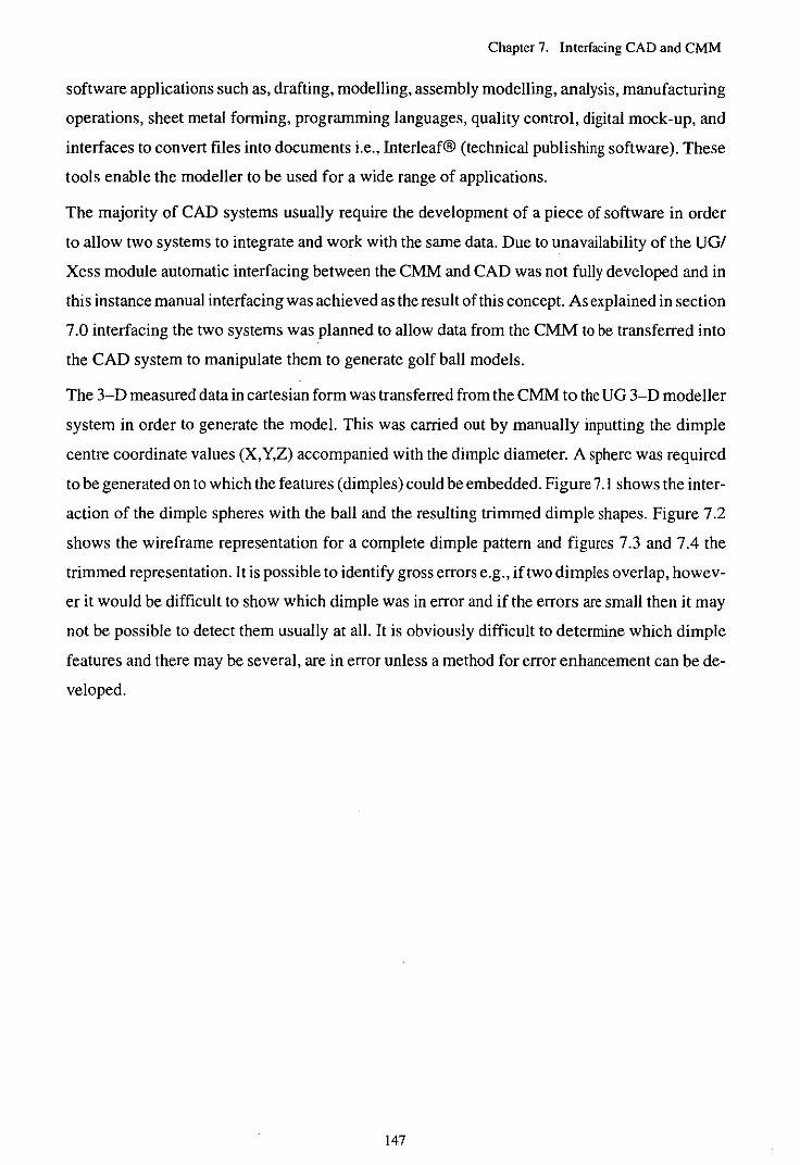
Chapter 7. Interfacing CAD and CMM
software applications such as, drafting, modelling, assembly modelling, analysis, manufacturing
operations, sheet metal forming, programming languages, quality control, digital mock-up, and
interfaces to convert files into documents i.e., Interleaf® (technical publishing software). These
tools enable the modeller to be used for a wide range of applications.
The majority of CAD systems usually require the development of a piece of software in order
to allow two systems to integrate and work with the same data. Due to unavailability of the UG!
Xess module automatic interfacing between the CMM and CAD was not fully developed and in
this instance manual interfacing was achieved as the result of this concept. As explained in section
7.0 interfacing the two systems was planned to allow data from the CMM to be transferred into
the CAD system to manipulate them to generate golf ball models.
The 3-D measured data in cartesian form was transferred from the CMM to the UG 3-D modeller
system in order to generate the model. This was carried out by manually inputting the dimple
centre coordinate values (X, Y,Z) accompanied with the dimple diameter. A sphere was required
to be generated on to which the features (dimples) could be embedded. Figure 7.1 shows the inter
action of the dimple spheres with the ball and the resulting trimmed dimple shapes. Figure 7.2
shows the wireframe representation for a complete dimple pattern and figures 7.3 and 7.4 the
trimmed representation. It is possible to identify gross errors e.g., if two dimples overlap, howev
er it would be difficult to show which dimple was in error and if the errors are small then it may
not be possible to detect them usually at all. It is obviously difficult to determine which dimple
features and there may be several, are in error unless a method for error enhancement can be de
veloped.
147
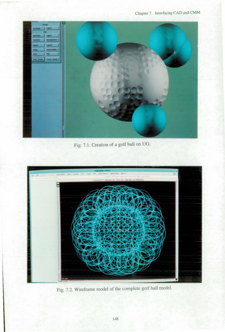
Chapter 7. Interfacing CAD and CMM
Fig. 7.1. Creation of a golf ball on UG.
- .
Fig. 7.2. Wireframe model of the complete golf ball model.
148
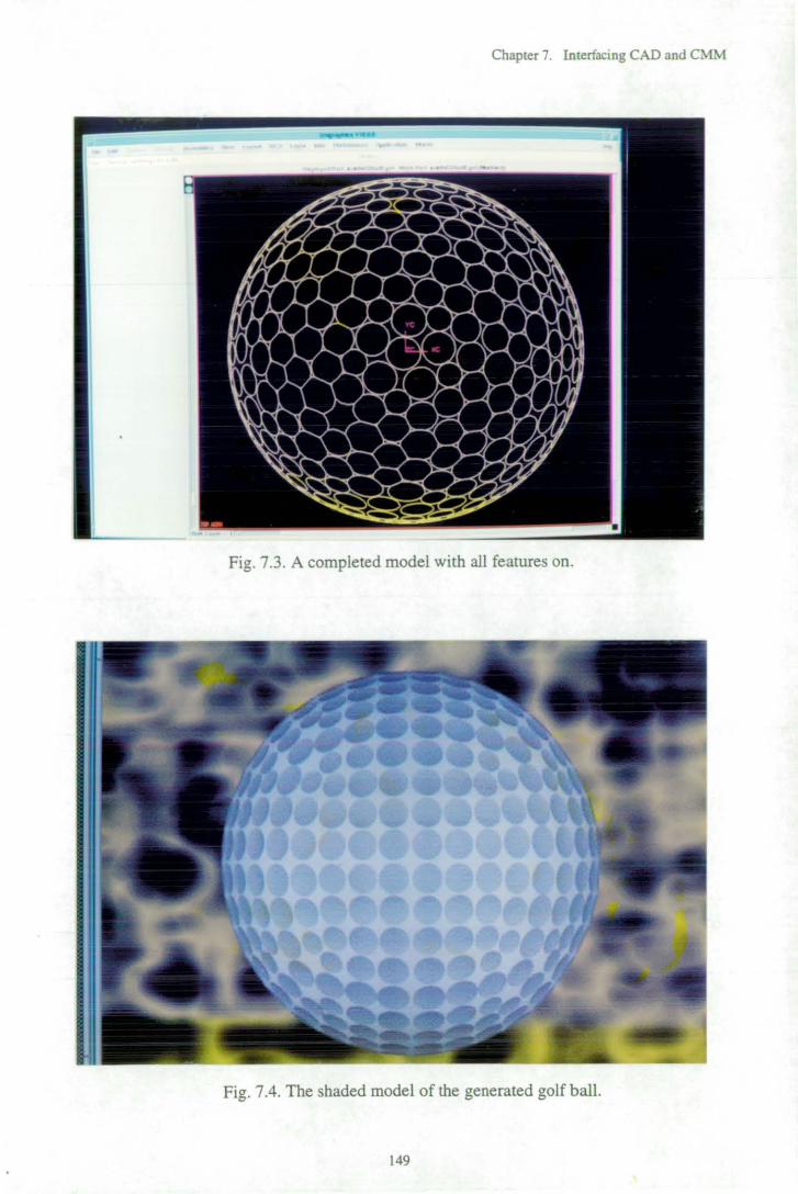
Chapter 7. Interfacing CAD and CMM
Fig. 7.3. A completed model with all features on.
Fig. 7.4. The shaded model of the generated golf ball.
149
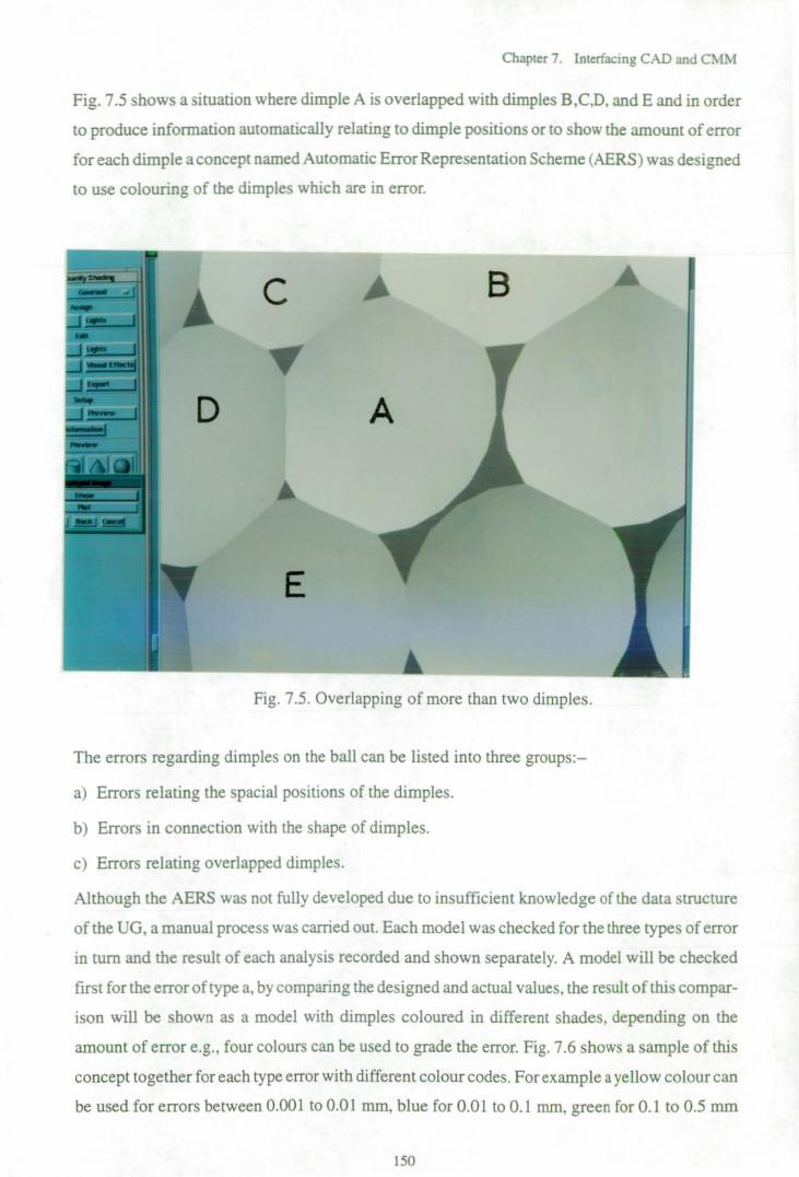
Chapter 7. Interfacing CAD and CMM
Fig. 7.5 shows a situation where dimple A is overlapped with dimples B,C,D, and E and in order
to produce information automatically relating to dimple positions or to show the amount of error
for each dimple a concept named Automatic Error Representation Scheme (AERS) was designed
to use colouring of the dimples which are in error.
c B
D A
E
Fig. 7.5. Overlapping of more than two dimples.
The errors regarding dimples on the ball can be listed into three groups:-
a) Errors relating the spacial positions of the dimples.
b) Errors in connection with the shape of dimples.
c) Errors relating overlapped dimples.
Although the AERS was not fully developed due to insufficient knowledge of the data structure
of the UG, a manual process was carried out. Each model was checked for the three types of error
in turn and the result of each analysis recorded and shown separately. A model will be checked
first for the error of type a, by comparing the designed and actual values, the result of this compar
ison will be shown as a model with dimples coloured in different shades, depending on the
amount of error e.g., four colours can be used to grade the error. Fig. 7.6 shows a sample of this
concept together for each type error with different colour codes. For example a yellow colour can
be used for errors between 0.001 to 0.01 mm, blue for 0.01 to 0.1 mm, green for 0.1 to 0.5 mm
150
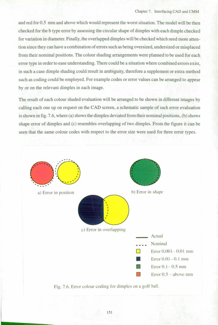
Cbapler 7. Inlerfacing CAD and CMM
and red for 0.5 mm and above which would represent the wor t situation. The model will be then
checked for the b type error by as e ing the circular shape of dimple with each dimple checked
for variation in diameter. Finally, the overlapped dimple will be checked which need more atten
tion since they can have a combination of errors such as being oversized, undersized or mi placed
from their nominal positions. The colour shading arrangements were planned to be used for each
error type in order to ease understanding. There could be a situation where combined errors exi t,
in such a case dimple shading could result in ambiguity, therefore a supplement or extra method
such as coding could be employed. For example codes or error values can be arranged to appear
by or on the relevant dimples in each image.
The re ult of each colour shaded evaluation will be arranged to be shown in different images by
calling each one up on request on the CAD screen, a schematic sample of such error evaluation
is shown in fig. 7.6, where Ca) shows the dimple deviated from theirnominal positions, (b) shows
shape error of dimples and (c) resembles overlapping of two dimples. From the figure it can be
seen that the same colour codes with respect to the error size were used for three error types.
0··----
• • • • • • • • • -- ...... ~
a) Error in position b) EITor in shape
cl Error in overlapping
- ctual
Nominal
o Error O.OOI- O.Ol mm
• ErrorO.Ol- O.l mm
11 Error O.l - 0.5 mm
Error 0.5 - above mm
Fig. 7.6. En'or colour coding for dimples on a go lf ball.
151

Chapter 7: Interfacing CAD and CMM
7.5 Machine code generation for an oDtimised measurement
The generation of machine code for CNC CMMs can be a laborious process and when it is done
correctly can have a direct effect on time saving for machining operations. In CNC measurement
the probe samples specific regions of the part and does not cover all areas as in machining. There
fore code generation for an optimised measurement requires suitable path planning and probing
strategy.
The area of path planning for CMM automatic inspection has been studied in recent years, es
pecially for parts having complex geometry such as dies and moulds. Automated planning of a
collision free inspection path using CAD model information requires a hierarchical planning sys
tem and automatic selection of probe angle for particular features. The principle of generating
inspection paths for a CMM requires analysing the geometry of the existing part model in order
to determine the measurement points. The inspection path can then be obtained by directly con
necting these measurement points with their clearance points. However, due to the complexity
of most CAD measurement system structures the generated inspection path is more easily created
for relatively simple parts or features [10].
In order to achieve an inspection system the following steps are required to be considered. First
an inspection plan needs to be determined which consists of selection of a probe, orientation of
a probe based on accessibility, and measurement locations including clearance point(s) for each
feature. Secondly the inspection procedure needs to determine the number of measurement points
required to ensure the feature quality. Once the above steps are completed the collision detection
for each individual path segment needs implementing
As mentioned in earlier chapters CAD and CMM links have been set up in recent years through
a DMIS format which gives a bidirectional data exchange standard [37] between the two systems
by creating a neutral file format for inspection programmes to be down loaded to the CMM and
for data following inspection to be sent back to the CAD system for analysis. An example of this
is Brown and Sharp's Microquindos and Mitutoyo's CMMCAD software. The packages are able
to import CAD data from a variety of CAD systems and present it in wireframe form to the user.
The user must identify and select all the features to be inspected, the software will then find each
feature in its database and calculate the necessary inspection points. The probe path is planned
for each feature, but collision detection is still left to the user to check during graphical simulation
of the programme.
Although advanced computer programming techniques for current CMMs are equipped with
various routines which enable them to be programmed for almost any measurement tasks, as yet
152

Chapter 7. Interfacing CAD and CMM
they are not as advanced as machining programming systems. They all require the part to be set
up and aligned on the machine table prior to the measurement.
Some of the important advantages of CAD driven CMM are the time savings which can be
achieved in comparison to that of a CMM on line programming technique. For example, in on
line programming the CMM needs to be stepped through its measurement routine in order to com
plete the programme and the CMM can not be used during development of the programme while,
within a CAD and CMM system the CMM can be continuously measuring with the old pro
gramme until the new program becomes available. Also through the CAD and CMM interface
a much easier analysis of the measured results can be performed, for example the user may learn
where to better sample the surface and how to interpret the results.
To drive a CMM from a CAD system the first step is to set up the part database which contains
both actual and measured data. The next step is to use the commands to build up the part pro
gramme. Path planning can be di vided into two section [37], sequence of probing and clash avoid
ance. In the former the datum features should be inspected first to establish the location of the
part in the work envelope. The probing points on a feature can then be selected with the aim of
achieving the minimum inspection time. Evaluation of measured data then requires fitting the
points to the corresponding features on the CAD model.
In essence an optimised measurement can be referred to as an automatic inspection procedure
which should support 3-D inspection, detect and prevent collisions of the trajectories of the probe
with the part and the selection of the measurement routes for the minimum inspection time.
7.6 Discussion
In this chapter a study of interfacing CAD and CMM has been presented along with the methods
for analysing the data generated by the inspection machine.
The current CMMs have been equipped with powerful softwares which allow them to produce
automated measurements, analysis, and also 2-D graphical representation. However, when the
part is complex or has a free form surface modelling of the part on the CMM becomes tedious
and often unsuccessful. The use of a robust modelling system such as a 3-D CAD modeller in
combination with a CMM may then be necessary for part or error representation.
Connecting these two systems together will allow the benefits of a CAD system for the CMM
measurement such as tolerancing and specifying the measuring approach direction together with
the possibility of intelligent inspection planning giving a Computer Integrated Manufacture
(CIM) environment.
153
Chapter 7. Interfacing CAD and CMM
A key factor to the future growth of CAD and CAI is the development of universal (versatile)
interfaces for design, inspection, and manufacturing applications. Although progress has been
made, CAD and CMM interfacing still needs further development to achieve higher flexibility,
intelligent inspection and enhanced automation. The future of CAD and CMM is bright, with the
price of hardware continually decreasing while the CAD's speed and CMM performance are in
creasing.
As discussed earlier the most effective interfacing solution for CAD and CMM systems is to have
and use an universal translator between the different type of CMMs. Apart from the obvious ver
satility benefits, such as the increase in the measurement quality by eliminating manually inten
sive data entry techniques and increases in machine availability, this solution has the advantage
that all measuring systems will have similar specifications. This process has already started with
the development ofDMIS which is evolving to maintain upward compatibility with IGESIPDES/
STEP standards developments [38], where an inspection file can be produced from scratch and
exported into any CAD/CAM system.
Through the CMMlCAD/CAI interface, programming efforts can be placed in the quality assur
ance office enabling a response to engineering product releases and change orders with new and
updated inspection data required to meet manufacturing needs [38]. From the CAD and CMM
link not only can an inspection strategy be implemented, but also a more strict regime can be in
troduced to diagnose the cause of problems after errors have been detected.
The accurate and automatic inspection of curved surfaces has not received significant attention
and due to changes of surface curvature in three axes accurate measurement can be difficult. The
number of such surfaces found in the aerospace industry alone means that the inspection of com
plex and curved surfaces is a critical part of the manufacturing process, and traditional methods
of inspection are time consuming and limited in application [133]. At present there are always
some elements remaining to be defined by the user such as, which part and feature should be in
spected, to what degree of precision, and a strategy for doing so [39].
Unless there is a gross error in dimples so that one dimple cuts another one, it is very difficult
to detect that through a CAD visual representation. The majority of the errors relating to dimples
on a ball are small therefore a colour shading arrangement (explained earlier) which depends
upon the error size may be an ideal method. This method can easily show the errors relating the
spatial positions, the shape and the overlapped dimples. Once the model is evaluated the result
of the analyses can be shown graphically on the CAD monitor.
154
Chapter 8. Discussion
CHAPTERS
DISCUSSION
Automated inspection and measurement of complex, free form or sculptured products to high
orders of accuracy is a laborious and ti~e consuming process, since for exact specification an
almost infinite number of points would be required. One of the most effective way of measuring
these products is by the use of a CMM but in order to measure or sense a feature or a surface it's
location needs to be identified. One possible way of identifying these locations is by employing
a perception system, such as a vision machine.
Vision systems are being used increasingly to automate the measuring processes and their use can
help to identify product shape and features but unfortunately for high accuracy their cost is pro
hibitive. If an integrated inspection system could be developed which could identify the surface
features quickly, then measure them to high accuracy with speed and suitable analysis the above
mentioned problems could be avoided. Such a system was developed in this work which consists
of an inexpensive 2-D machine vision with a CNC CMM incorporating probing.
Several experiments were performed to demonstrate the effectiveness of the proposed methods,
and the results show that the automated inspection for sculptured surfaces can be achieved suc
cessfully with reduced cost. The following discussions are based on the experiments carried out
during this work which have led to a set of guide lines for operation.
• Feature specification. One of the main problems when looking at features using a vision
system is determining the extent of features. In prismatic parts distinct edges are present which
identify a feature and it is also possible to construct the feature shape by implication from the
feature locations, for example intersection of planes. The specification of features for sculptured
parts is uncertain due to not knowing the general shape of the features or the extent, generally
lines or grids are marked onto the surface to identify features or patches.
It is apparent that there are no generic solutions for automated feature identification and detec
tion, and one way of developing methods is by investigating special cases in order to learn rules
and methods which can be applied elsewhere (e.g., shoe last inspection etc.). The selected objects
in this work were golf balls which are special cases of multi faceted feature parts albeit positioned
around a regular object sphere. For simple balls the dimple shape would be constant (one dimple
shape repeated around the whole ball), whereas complex balls can have as many as eleven dimple
sizes.
A number of techniques were used to develop a simple method for feature detection by the use
of a 2-D vision system and it was found that feature marking was the most suitable for the pur-
155

Chapter 8. Discussion
pose. This method was based on human or industry perception of the feature and then manual I y
placing a small mark (dot) inside of each feature with a marker pen.
• Feature detection and enhancement by 2-D machine vision. As mentioned earlier, feature
identification can be the most difficult section of a detection system and one of the main reasons
is that features for sculptured parts are usually 3-D with no detectable edges or having primitive
shapes. In order to identify the location of the surface features for sculptured surfaces and in
special cases when the surface could have many features, a fast detection and reliable method is
required. Using a machine vision the information which could lead to the recognition of the fea
tures could be interpreted from shadows, surface discontinuities and suitable lighting. However,
this is a subjective process.
3-D feature identification methods are available [25,28] but expensive and complex and the com
mon industrial vision systems are 2-D making depth determination difficult. One solution for
feature determination is to enhance them for easy identification by a vision system. A marking
method can determine the approximate position of the features regardless of their shapes or
orientations. As remarked earlier, with a prior knowledge of the feature shape it was possible to
detect and locate the marks by a set of developed algorithms and softwares which then allowed
the evaluation of the features to the highest CMM accuracy. This method proved to be very simple
and effective and may possibly be used elsewhere with some modifications to the system in order
to be applicable to other forms of sculptured surfaces such as turbine blades, shoe lasts, golf clubs
etc. A limitation with the technique is the ability to place the identification mark in the approxi
mate centre of the feature .
• Feature identification in 3-D. One of the main problems with the use of a 2-D vision system
for feature detection is determining the feature height in relation to a datum surface or reference
point. Three methods were initially considered, Z-layer, segmentation and 3-D calculation. The
main problem with the Z-Iayer approach is selecting layers such that they contain complete fea
tures i.e., dimples. Dimple patterns do not follow such rigid rules and any layer selected will inev
itably cut through some dimples. To a reduced extent this problem is also apparent with the seg
mentation method since the segments contain layers.
To reduce the complexity of the 3-D calculation of dimple positions and by knowing that these
features are always on a spherical object it was found more appropriate to move the vision system
reference point from the top left corner of the image to the centre of the ball or hob. The height
of the dimple is generally dependent on its' distance from the ball centre and it was assumed that
the dimple centre lies on the ball sphere with a known radius. It was then possible to calculate
the approximate Z-heights of the identification dots using trigonometry.
156
Chapter 8. Discussion
When an optical 2-D vision system is used to represent a 3-D data point some discrepancy be
tween the measured and the optical values will be generated. This optical discrepancy acts
radially from a point vertically above the object centre. In this work a 2-D correction factor was
developed to compensate for this optical effect. Although this was developed and tested for golf
balls it was not used since the calculated centres were adequate for the measurement process for
larger objects a correction would have to be used .
• Multi-image feature detection. It is obvious for efficient feature detection to use only one
camera position. However, when one camera position was considered, it was found that the fea
tures in areas where the surface curvature changed rapidly tended to merge together and on the
outer extreme of the ball could not be detected. Therefore, multi-images were used in order to
identify features in these areas. The generated technique (MIST) viewed the object of interest a
number of times from different directions and combined the information, for curved objects it
is likely that there will be areas which could be identified more than once. In the case of the golf
ball these areas were created by overlapping up to three neighbouring images of the surface.
In order to minimise the number of views it is necessary to have some confidence in the informa
tion available in anyone image. In the case of the golf ball confidence in feature identification
diminishes away from the ball centre. The dimples that can be identified with confidence can be
contained with an approximate circular area or ring of about 18.5 mm radius. In this work 5 views
were used to develop the methods. The situation for 100 per cent ball cover is shown in fig 5.6
which gives a radius of 17.51 mm. Fortunately all dimples in these areas can be confidently
identified which might not be the case for more complex products. Ideally the overlapped areas
shown in fig. 5.6 should be kept as small as possible. Despite the fact that the data sorting algo
rithms were developed to censor the detected repeated data sets, this could not guarantee 100 per
cent sorting. The method applied to the cubic golf balls by using 17.51 mm radius image ring to
detect 220 dimples on a half ball which resulted in about 50 per cent of the dimples being identi
fied more than once .
• Data sorting and censorship. With the use of MIST the generation of repeated dimples was
inevitable and in order to keep the inspection time to a minimum, a procedure was needed to
measure each dimple once only. It was found more efficient to sort a complete data file after all
dimples were detected, which enabled repeated dimples to be censored. Various golf balls were
tested with the data sorting method (the DimSort programme explained in chapter 5) with the
machine under continuous supervision in order to control the method efficiently. Up to 90 per
cent of the repeated data was detected and an average value substituted leaving the remaining 10
157
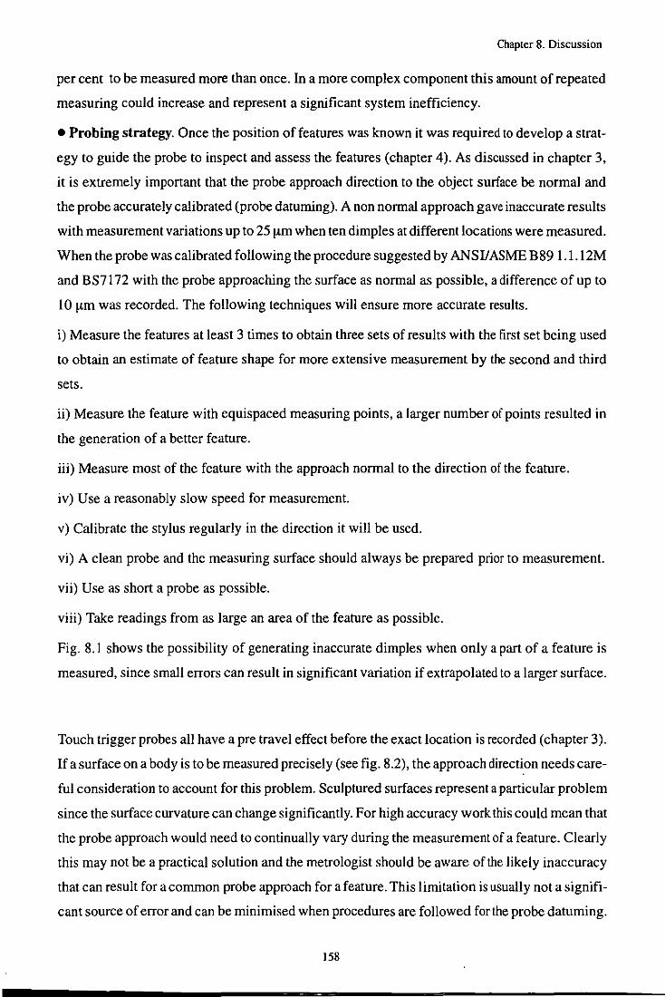
Chapter 8. Discussion
per cent to be measured more than once. In a more complex component this amount of repeated
measuring could increase and represent a significant system inefficiency .
• Probing strategy. Once the position of features was known it was required to develop a strat
egy to guide the probe to inspect and assess the features (chapter 4). As discussed in chapter 3,
it is extremely important that the probe approach direction to the object surface be normal and
the probe accurately calibrated (probe datuming). A non normal approach gave inaccurate results
with measurement variations up to 25 !lm when ten dimples at different locations were measured.
When the probe was calibrated following the procedure suggested by ANSI/ ASME B89 1.1.12M
and BS7172 with the probe approaching the surface as normal as possible, a difference of up to
10 !lm was recorded. The following techniques will ensure more accurate results.
i) Measure the features at least 3 times to obtain three sets of results with the first set being used
to obtain an estimate of feature shape for more extensive measurement by the second and third
sets.
ii) Measure the feature with equispaced measuring points, a larger number of points resulted in
the generation of a better feature.
iii) Measure most of the feature with the approach normal to the direction of the feature.
iv) Use a reasonably slow speed for measurement.
v) Calibrate the stylus regularly in the direction it will be used.
vi) A clean probe and the measuring surface should always be prepared prior to measurement.
vii) Use as short a probe as possible.
viii) Take readings from as large an area of the feature as possible.
Fig. 8.1 shows the possibility of generating inaccurate dimples when only a part of a feature is
measured, since small errors can result in significant variation if extrapolated to a larger surface.
Touch trigger probes all have a pre travel effect before the exact location is recorded (chapter 3).
If a surface on a body is to be measured precisely (see fig. 8.2), the approach direction needs care
ful consideration to account for this problem. Sculptured surfaces represent a particular problem
since the surface curvature can change significantly. For high accuracy work this could mean that
the probe approach would need to continually vary during the measurement of a feature. Clearly
this may not be a practical solution and the metrologist should be aware of the likely inaccuracy
that can result for a common probe approach for a feature. This limitation is usually not a signifi
cant source of error and can be minimised when procedures are followed for the probe datuming.
158
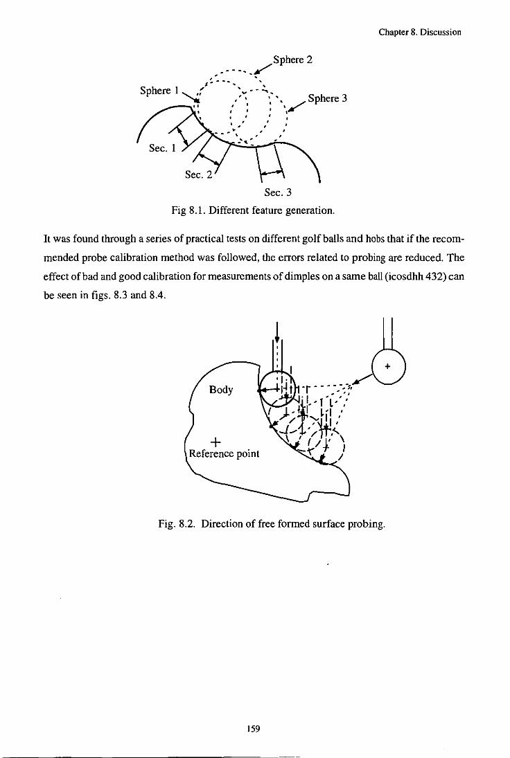
Chapter 8. Discussion
Sphere 2 --- ... / - . s ~ - ....... ..
Sphere 1 '- ,;' • v - - :.. ...... I' \ :" .. .. Sphere 3
..... - ..... , , I ,./ f •• ,~ , , -'
Sec. 3
Fig 8.1. Different feature generation.
It was found through a series of practical tests on different golf balls and hobs that if the recom
mended probe calibration method was followed, the errors related to probing are reduced. The
effect of bad and good calibration for measurements of dimples on a same ball (icosdhh 432) can
be seen in figs. 8.3 and 8.4.
Fig. 8.2. Direction of free formed surface probing.
159
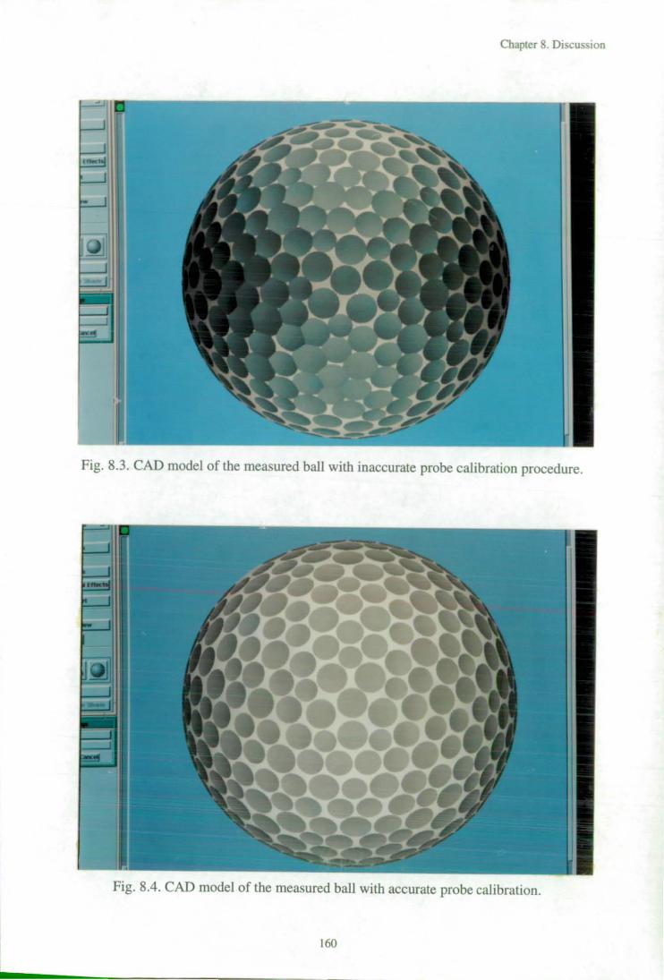
Chapter 8. Discussion
Fig. 8.3. CAD model of the measured ball with inaccurate probe calibration procedure.
Fig. 8.4. CAD model of the measured ball with accurate probe calibration.
160
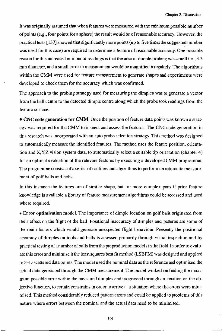
Chapter 8. Discussion
It was originally assumed that when features were measured with the minimum possible number
of points (e.g., four points for a sphere) the result would be ofreasonable accuracy. However, the
practical tests [137] showed that significantly more points (up to five times the suggested number
was used for this case) are required to determine a feature of reasonable accuracy. One possible
reason for this increased number of readings is that the area of dimple probing was small i.e., 3.5
mm diameter, and a small error in measurement would be magnified irregularly. The algorithms
within the CMM were used for feature measurement to generate shapes and experiments were
developed to check them for the accuracy which was confirmed.
The approach to the probing strategy used for measuring the dimples was to generate a vector
from the ball centre to the detected dimple centre along which the probe took readings from the
feature surface .
• CNC code generation for CMM. Once the position of feature data points was known a strat
egy was required for the CMM to inspect and assess the features. The CNC code generation in
this research was incorporated with an auto probe selection strategy. This method was designed
to automatically measure the identified features. The method uses the feature position, orienta
tion and X,Y,Z vision system data, to automatically select a suitable tip orientation (chapter 4)
for an optimal evaluation of the relevant features by executing a developed CMM programme.
The programme consists of a series of routines and algorithms to perform an automatic measure
ment of golf balls and hobs.
In this instance the features are of similar shape, but for more complex parts if prior feature
knowledge is available a library of feature measurement algorithms could be accessed and used
where required .
• Error optimisation model. The importance of dimple location on golf balls originated from
their effect on the flight of the ball. Positional inaccuracy of dimples and patterns are some of
the main factors which would generate unexpected flight behaviour. Presently the positional
accuracy of dimples on tools and balls is assessed primarily through visual inspection and by
practical testing of a number of balls from the preproduction models in the field. In order to evalu
ate this error and minimise it the least squares best fit method (LSBFM) was designed and applied
to 3-D scattered data points. The model used the nominal data as the reference and optimised the
actual data generated through the CMM measurement. The model worked on finding the maxi
mum possible error within the measured dimples and progressed through an iteration on the ob
jective function, to certain constrains in order to arrive at a situation where the errors were mini
mised. This method considerably reduced pattern errors and could be applied to problems of this
nature where errors between the nominal and the actual data need to be minimised.
161
Chapter 8. Discussion
The LSBFM was found to be simple and successful due to its fast processing time and ease of
appreciation. The main shortcomings of this method can be broadly listed as; a) not showing the
direction of errors from which possible relationships could be found, and b) it is not integrated
into the VG CAD system in order to perform an automatic graphical representation. However,
error model tests for two hobs were successfully carried out and the results were studied manually
(two sets of results can be seen in appendix A). A total of 220 and 213 dimples were measured
on the two hobs used. The nominal and measured values were fed into the error modelling system
in order to produce an optimise model. The results of these tests were the optimised locations for
the measured dimples with an average error reduction of about 40 per cent. From the results (ap
pendix A) the maximum and minimum error variations between the error lengths of CAD -CM M
and CAD-optimised values for the cubic hob were recorded as 7.7 !lm, 1.0!lm and those for the
icosdhh432 hob were 4.6 !lm, and 1.1 !lm .
• Virtues of this work. The research advances the 3-D automatic inspection of features on sculp
tured surface products through the application to a specific product. Although the system was
applied to golf balls which are complex products to inspect, it could be applied to other products
which can be featurised and which have not been measured automatically to date e.g., golf clubs,
bottles, and shoe lasts.
The proposed integrated inspection system has the following virtues,
i) A lOO per cent surface feature detection,
ii) Measurementtime saving up to 10 times in comparison to the conventional method with mini
mum operator interference,
iii) An accurate measurement consistency to a few microns for all the features,
iv) Simplicity of the surface feature detection and measurement procedures,
v) An inexpensive and effective system in comparison to other rival systems.
162

Chapter 9. Conclusions
CHAPTER 9
CONCLUSIONS
This research presents a developed method of automated inspection for sculptured surface prod
ucts by integrating a CMM and 2-D vision system. The research outlined in this work may be
applied to free formed surfaces but some modifications such as specifying reference points for
the surfaces needs to be developed. The system was developed on golfballs which are considered
to be a special instance of a product with surface features. The conclusions can be summarised
as follows:-
• Automated identification of surface features is difficult for sculptured surface products.
• Careful illumination of products can help enhance features particularly with the use of a fluor
escent light source and filtered light. A suitable illumination system was achieved by the use of
a fluorescent ring light and filtering using white paper filters.
• If prior knowledge of feature shapes is available, then a feature and its position can easily be
identified by the use of a small mark or dot in the approximate centre of the feature to an accuracy
of 0.2 mm.
• If prior know ledge of the part or feature is available using a single 2-D image of the part enables
a 3-D shape to be probed .
• It is possible to generate a library of probe measuring routines for feature types and apply them
to identify features automatically for accurate measurements, < 0.01 mm.
• The use of multiple images achieves a more comprehensive view of a product in particular for
areas of rapidly changing surface curvature and this allows 100 per cent surface/feature cover.
However it is necessary to censure formation in overlapped image areas to reduce repeated in
spection.
• The savings in measurement time for this "look and touch approach" compared to traditional
inspection methods can be considerable. In the cases investigated of dimples on golf balls saving
in the order of 10 times have been achieved.
• In order to assess component accuracy datums are required which are difficult to establish for
sculptured products. The method of fitting measured feature patterns to the design specification
163

Chapter 9. Conclusions
using a three dimensional least squares technique proved successful, the examples used reduced
the errors by 40 per cent.
• The use of a CAD modelling system to enhance component error by colour coding error types
has many advantages for unambiguous interpretation by operators.
164

Chapter 10. Recomendations for future work
CHAPTER 10
RECOMMENDATIONS FOR FUTURE WORK
In this research several topics were handled to implement an automated inspection of sculptured
surfaces with the use of a machine vision. Recommendations for future research in order to im
prove the proposed system are listed below:
• Optimisation of probe orientations. An optimisation method for probe orientations can be
employed in order to inspect features which could use the same probe orientation. This will re
duce the inspection time. Presently there is no control on the size of the marks placing inside of
the features which resulted in an unpredictable feature detection order, meaning they will be
measured in the order they were detected. A significant effect of this is the generation of too many
unnecessary probe movements. If a controlled feature detection or a feature sorting method could
be arranged in a way that grouping the features which could be probed with the same probe
orientation, the inspection time could be minimised.
• Feature identificationiMarking other sculptured parts. The feature identification method
is of interest and for multiplicity of features on a ball a more comprehensive method should be
investigated. The dot marking method proved successful for circular features, however a more
difficult case is when the features on the surface have more than one shape, for example dimple
shapes based on triangle, squares, pentagons, or a mixture of all. For such cases an advance mark
ing method is required to be developed in order to help the vision system to identify these features.
One way of arranging the advanced marking method could be using combined marks such as,
dots, arrows, triangles, crosses and other possible practical symbols. Routines and algorithms are
required for the vision and CMM to identify and process these marks.
• Optimum (reduced) view positions. Further practices should be developed for applying the
MIST to objects using an optimised view positions, in order to reduce the automated inspection
time further. This will be possible by using some trigonometric relationships between the camera
locations and the part coordinate system.
• Application of the MIST to other featurised sculptured parts. The proposed MIST should
be applied to other featurised sculptured parts (non-regular objects) such as a golf club or shoe
last which have not been measured automatically to date. A starting point for this is to use the
advance marking method. The approximated locations of these marks can then be determined by
referring them to one or different datums. The direction of these marks can also be identified by
using some developed algorithms within the detection method. This could be an answer to the
165
Chapter 10. Recomendations for future work
inspection or identification of complex free formed sculpture surfaces where specifying the
direction and the correct location of the patches and surfaces is one of the most difficult parts of
the process.
• Application of the MIST to prismatic parts. The MIST with the marking method can also
be applied to objects which consists of prismatic features such as blocks, pockets, spheres, bosses
etc., Although a number of researches [102] have been devoted to this area, the simplicity and
effectiveness of this method could justify it.
• Automated CAD model and error generation. The CAD generated models of the measured
balls and hobs should be researched further in order to use the VG/Xess (explained in chapter 7)
for automatic CAD modelling. This could also allow an automatic 3-D CAD representation of
errors using colour coding explained earlier on the optimised model on the UG CAD system.
• Illuminating the object. Although a solution was achieved for this case (explained in chapter
4), there is still further work to be carried on lighting methods and systems. One possible way
is to use diffuse lights around the workplace in order to create regular illumination. Another suc
cessful approach could be to use indirect lights by utilising umbrella reflection arrangements. The
above methods can be arranged to illuminate the object from a distance up to a few meters.
• Efficiency and probe motion. The CNC CMM code generation for feature measurement was
mainly considered with respect to taking successful measurements rather than optimising the
speed of measurt:ment. Work is required therefore on this aspect in order to speed up the process.
As explained earlier each dimple was probed three times (5,19, and 19) which gave 43 readings
and for a ball with 250 dimples a total of 10750 probings has to be carried out.
• The LSBFM errors analysis for other complex features. An additional area of research can
be developed by investigating the application of the LSBFM of error optimisation to surfaces of
other sculptured parts. In such a case a relationship for each patch or surface to a datum point and
consequently to a global (master) datum point needs establishing. By comparing the actual and
nominal data of each surface the possible error between them and also for the neighbouring
patches could be identified. Once the amount of errors are determined an optimisation method
could be applied.
• Future integration between CAD and CMM. A series of practical work needs carrying on
in the area of CAD and CMM integration in order to utilise the full ability of communication be
tween the VG CAD and Tesa CMM.
166
Chapter 11. References
REFERENCES
[1]. Batchelor B.G., Hill D.A., Hodgson D.e., AutoTlUlted VISual Inspection, pub. by IFS
(Publication) Ltd, U.K., 1985.
[2]. Elshennawy Ahamad K., The role of inspection in autoTlUlted TIUlnufacturing, Com
puters ind. Engineering 17(1-4), 1989. -
[3]. Berg B.VanDen, Closed loop inspection of sculptured surfaces in a computer integrated
environment, Proc. 8th 1nl. Conf. Automated inspection and product control 1, 1987.
[4]. Takeuchi Yoshimi, Shimizu Hiroyuki, Mukai Ikuo, AutoTlUlted Measurement of 3-Di
mensional Coordinate measuring Machine by means of CAD and ITIUlge Data, Annals of
the Int. Instituation for Prod. Eng. Research (CIRP) 3911190, 1990.
[5]. Gupta V.K., Sagar R., APC-based system integrating CMM and CAD for automated
inspection and Reverse engineering, Int. I. Advan. Manuf. Tech. (IJAMT), 1993.
[6]. AI-Kindi G.A., Baul R.M., Gill K.F., An example of automated two-4imensional com
ponent inspection using computer vision, IMechE 205, 1991.
[7]. Merat Francis L., Radack Gerald M., AutoTlUltic Inspection Planning Within a Feature
Based CAD System, Int. I. of Robatics & Comp.-Integ. Manuf. (IJRCIM) 9 No.1, 1992.
[8]. Mahon lames, Automatic 3-D inspection of solder paste on surface mount printed cir
cuit boards, 1nt. I. Materials Processing Technology (IMPT) 26, 1991.
[9]. Zarifi A., lones R., Automated Measurement of Golf Balls Using Machine VISion As
sistance, I. of Quality of world Today Supplement (QWTS), March, 1994.
[10]. Yau Hong-Tzong, Menq Chia-Hsiang, Path Planning for Automated Dimensional In
spection Using Coordinate Measuring Machines, Int. Conf. on Robotics and Automation
(IEEE), 1991.
[11]. Corrigall M.I., Bell R., Probe and Component Set-up Planning for Coordinate
Measuring Machines, Int. J. ofComp. Integ. Manuf. (IJCIM) 4 No.!, 1991.
[12]. Cho H.D., lun T.T., Yang M.Y., Five-axis CNC milling for effective machining of
sculptured surfaces, Int. I. of Production and Research (IJPR), 1993.
[13]. Brown and Sharp Company, TESA CMM Publication, 1993.
[14]. Ferranti International Ltd. Scotland U.K. The Merlin CMM manual, 1988.
[15]. Sarkar Biplab, Menq Chia-Hsiang, Scanning compound surfaces with no existing
167
Chapter 11. References
CAD model using touch probe of a Coordinate Measuring Machine, Intelligent Design and
Manufacturing for prototyping (IDMP) 50 (PED) Winter ASME, 1991.
[16]. 3D Scanner Ltd., FACIA: Medical Surface Scanner, 3D Scanners Lld South Bank
Technopark 90 London Rd SE1 6LN, 1991.
[17]. Champ Peter, Reverse Engineering in Industrial Applications using Laser stripe Tri
angulation, Colloquium digest No. 1994/054, lEE, March, 1994.
[18]. Duffie N., Bollinger J., Riper R., Kroneberg M., CAD directed inspection and error
analysis using surface patch databases, CIRP 33-No.1, 1984.
[19]. Duffie N., CAD directed inspection and error patch databases, CIRP 33-No.1, 1987.
[20]. Smith D., Touch Probe Attack Angle Problems, Quality Today, Sept. 1987.
[21]. Butler Clive, An investigation into the performance of probes on coordinate measur
ing machines. Industrial Metrology 2-part4, 1991.
[22]. Zuech Nello, Applying Machine VISion, John Wiley and Sons, Inc. ed. John Wiley and
Sons, U.S.A., 1988.
[23]. McMichael D., Fusing Multiple Images and Extracting Features for VISual Inspec
tion, lEE Factory 2000, 1992.
[24]. Schneider Carl., Sinnreich Kurt, Concept of an optical coordinate measurement ma
chine, SPlE 1395, 1990.
[25]. Clarke T.A., Ellis TJ., Robson S., High accuracy 3-D measurement using multiple
camera views, Colloquium digest No. 1994/054" lEE, March, 1994.
[26]. Urquhart c.w., McDonald J.P., Fryer R. J., Active Animate Stereo VISion, British Ma
chine Vision Conference (BMVC) 1,1993.
[27]. Seibert Michael, Waxman Alien M., Adaptive 3-D object Recognition/rom Multiple
Views, lEEE Trans. Patt. Anal. Machine Intelligent., Vol. 14, No. 2, 1992.
[28]. McDonald I.P., Lambert R., Fryer RJ., 3D Measurement Using Stereo Scene Coding,
lEE. Colloquium digest No. 1994/054, March, 1994.
[29]. Griffiths BJ., Wang Y., Wilkie B., AI VISion for Inspection, ACME WISEACME.002,
1993.
[30]. Scalkoff Robert J, Digital Image Processing and Computer VISion, John Wiley & Sons,
Inc. New York, 1994.
[31]. Gonzalez Rafael C., Woods Richrd E., Digital Image Processing, Addison-Wesley
168
I
Chapter 11. References
Publishing Company, Inc., Reading., 1992.
[32]. Wolf Paul R., Elements of Photogrammetry, 2nd. Ed. Vol. 1. McGraw-Hill, Inc. 1983.
[33]. Martin W.N., Aggarwal J.K., Volumetric descriptions of objects from multiple views,
IEEE Trans. Patt. Anal. Machine Intelligent., Vol. 5, No.2, 1983.
[34]. Liu Cheng Hsiung, Tasi Wen Hsiang, 3D Curved Object Recognition from Multiple 2D
Camera Views,. Computer Vision Graphics and Image Processing 50, 1990.
[35]. Edwards J., Clements P., Murgatroyd S., Machine vision integration and information
support: methods, models and tools, Int. J. of CIM, Vol. 6, No. 5, 1993.
[36]. Cho M.W., Kim M.K., Kim K., Flexible Inspection System Based on VISion Guided
Coordinate Measuring Machine, InU.Prod.Res. (IJPR),Vol. 33, No. 5, 1995.
[37]. Harris J.R., Rockliffe S.c., Smith G., Hill T.M., A review of on-line and off-line pro
gramming facilities for coordinate measuring machines, Factory 2000, 1994.
[38]. Daniels Glynne E., DMIS: a quality Standard, J. of Quality Today, January 1992.
[39]. Cowling G.J., Mullineux G., Toward an Intelligent CAD-CMM Interface, Engineering
with Computers 5, 1989.
[40]. Schartz Mark H., Karadayi Recep, Making the CAD to CMM Interface More Effective,
Society of Manufacturing Engineers (SME), MS89-530, 1989.
[41]. Fu K.S., Gonzalez R.c., Lee C.S.G., Robotic control, Sensing and intelligence,
McGraw-Hill International Editions, New York, 1988.
[42]. Frost and Sullivan, Machine Vision, Engineer Technical File No. 223, August 1993.
[43]. Sension Advanced Computing, Advance Computing News, Kane International Limited,
7 Craftwood Square, Martland Mill Industrial Estate, Wigan, WN5 OLG, 1994.
[44]. Data Cell Co., Image Matters 2, Newsletter, 1994, West End Rd, Mortimer Common,
Reading, Berks RG7 3TF, U.K.
[45]. Taylor Barry, Placement: VISion and Integration, Electronics Manufacture and Test
July/August 1991.
[46]. Purnell G., Khodabandehloo K., VISion for Robot Guidance in Automated Butchery, J.
of Robotic Systems, Advanced Techniques and Applications 10, 1992.
[47]. Azar I., Weston R.H., A vision reference modelforsystems integration, Int. J. of
CIM, 1 No. 4,1992.
169
Chapter 11. References
[48]. Svetkoff DJ., Smith D.N., Doss B.L., Automatic Inspection of Component Boards
Using 3-D and Greyscale VISion, Microelectronics 13, 1987.
[49]. Blacke Andrew, Double Grid Maps 3D Shapes Precisely, Eureka on Campus Autum,
53,1991.
[50]. Brown Joe, VISion Systems Get Better at Doing What Eyes Can't, Power Transmisson
Design 5, 1991.
[51]. Pastorius W.1., Robots in Aerospace Manufacturing, SME MS89-162, 1989.
[52]. Harding Kevin G., Sensors for '90s, Mechanical Engineering 106, part 4, 1991.
[53]. MVP-AT user's manual. Matrox Electronic Systems Limited, 1988.
[54]. Grover M.P., Weiss M., Nagel R.N., and Odrey N.G.lndustrial Robotics, McGraw-HiII
International Editions, 1988.
[55]. McCarthy Brian, Genest David H, Getting your CMMs and CAD system to talk, Ma
chine and Tool Blue book 85 part 6, 1990.
[56]. Graund Bill, Maggiano Larry, Smart Contact Scanning, Conf. Applying Irnaging and
Sensoring technology to CMM Applications, Pub. SME, 1993.
[57]]. Genest David H., Coordinate Measuring Machines, Inspection Equipement and Tech
niques, Brawn & Sharps Publication, U.S.A., 1993.
[58]. Renishaw CMM product Group 4, General Product, Bulletin, 1992.
[59]. ANSUASME B89 1.l.12M, The American National Standard For Coordinate
Measuring Machine, 1989.
[60]. Reid Colinperformance Characteristics of Touch Trigger Probes. Renishaw Metrology
Publication U.K. 1993.
[61]. Traylor Alan, Jarman Tom, Performance Characteristics of Touch Trigger Probes,
SME MS90-266, U.K.,1990.
[62]. Modjarrad Amir and Dukiewicz Peter, Development of a small novel 3-Dimensional
high accuracy probe for CMMs, Quality Europe 36, Part I, U.K., 1991.
[63]. Reid Colin, Probe Technology Beyond Accuracy, Conf. Applying Irnaging and Sensor
ing technology to CMM Applications, SME Pub., 1993.
[64]. Fitts John M., Miniature 3D surface mapping moire sensors for the CMM, Applying
irnaging and sensoring technology to CMM applications I, U.S.A., 1993.
170
Chapter 11. References
[65]. Owen Jean V, Are Laser Measuring Up? Manufacturiing Engineering 104 part 1, Jan
uary 1990.
[66]. Kunzmann H., Walde1e E, Performance of CM Ms, CIRP 37-No.2, 1988.
[67]. Danzer H.H., Kunzmann H., Application of 3-Dimensional Coordinate Measuring
Machines for problem Investigation and upstream quality assurance, CIRP 36-1,1987.
[68]. Paolino Richard E, Genest David H., Justifying the CMM, Carbide and Tool Journal,
21 part 4, 1989.
[69]. Daschbach James M., Sairamchandar R.,S., Coordinate Measuring Tool, SME
MS89-528, 1989.
[70]. Oetjens Thomas J., New Developments in Coordinate Measuring Machinesfor Sheet
Metal, Autofact 19,1989.
[71]. Cox M.G., Assessing CMM software quality, J. of Quality Today, January 1992.
[72]. Goh K.H., Bell R., The applicability of a Laser triangulation probe to non-contacting
inspection. Int. J. Prod. Res. (IJPR),Vol. 24 No.6, 1986.
[73]. Bradley c., Vickers G.w., Milroy M., Reverse Engineering of Quadric Surfaces Em
ploying three-dimensional Laser scanning, Inistitue of Mechanical Engineering 208, 1994.
[74]. Dalgleish G.F., James R.D., Randeree K.H., Aitchison D.R., Laser-Based inspection of
cutting tools for advanced manufacturing systems, Factory 2000 October, 1994.
[75]. Farmer L. E., Smith G., Integrating CAD and CMM Inspection, Inernational Mechani
cal Engineering Congress 91 part 8, 1991.
[76]. Pahk H.J., Kim Y.H., Hong Y.S., Kim S.G., Development of Computer Aided Inspec
tion System with CMM for Integrated Mold Manufacturing, CIRP 42-1, 1993.
[77]. Oh kaytack, Daschbach James M., Abella Robert J., CMM Application in Reverse En
gineering-Integrating CMM With CAD/CAM for Exisying Parts Without Drawings, SME
MS89-529, MS89-529-1 MS89-529-9 1989.
[78]. Kwok Wai-Lun., Eagle Paul J., Reverse Engineering: Extracting CAD Data From Ex
isting Parts, Mechanical Engineering 113 part 3, 1991.
[79]. Renishaw Ltd. High Speed Scanning of 3-D Surfaces. Quality Today Januaray, 1992.
[80]. Spokes Ben, CMM - Style Machine Tool Inspection Probing, Final year undergraduate
project Manufacturing Eng. Dept., Loughborough University, U.K., 1993.
[81]. Morton Danny, Systematic and spatial errors, their measurement and compensation
171
Chapter 11. References
method applid to CMMs, School of Eng., Huddesfield University, U.K. 1994.
[82]. Brown & Sharpe, Measuring equipment Catalogue, Brown & Sharpe Pub., Tesa Me
trology Ltd., Telford, Shropshire, U.K. 1994.
[83]. Dallas D.B., Tool and Manufacturing Engineering Hand Book, 3rd Edition, Pub. by
SME,1976.
[84]. W.A. Metrology pub. U.K., 1993.
[85]. Zink Joseph H., The Role of Coordinate Measuring Machines in Assuring Quality,
Computer Integrated Manufacture REVIEW Summer, 1988.
[86]. Palframan Diane, At Last Industry Can, J. of Manuf. Sys., April 1993.
[87]. Jones R., Mitchell S.R., Newman S.T., Feature-Based Systems for the Design and
Manufacture of Sculptured Products, Int. J. Prod. Res., Vol.31 ,No.6, 1993.
[88]. Mitchell S.R., Jones R., Newman S.T., A Structured Approach to the Design of Shoe
Lasts, Journal of Engineering Design, Vo1.6, No.2, 1995.
[89]. Olman John M., Olman Morton w., The Encyclopedia ofGolfCollectibles, Books Am
ericana Inc., 1985.
[90]. Pinner John, The History of Golf, The Apple Press Ltd., 1988.
[91]. The Royal and Ancient Golf Club of St. Andrews, Rules of Golf, 1991.
[92]. Daish B.C., The Physics of Ball Games, English University Press, 1972.
[93]. Wenninger Magnus J., Dual Models, 1st Ed., Cambridge University Press, 1983.
[94]. Blake A., McCowen D., Lo H.R., Lindsey P.J., Trinocular Active Range-Sensing. Uni
versity of Oxford Dept. of Engineering Science, 1991.
[95]. Celenk Mehmet, Bachnak Rafic A., Multiple Stereo VISion System For 3-D Object Re
construction, Jour. of Applied Systems Analysis, 1990.
[96]. B1isset R.J., Stephens M.J., Sparks E.P., Surface Perception and Localisation Using
Passive VISion, 9th Int. Conf. Automation Inspection & Product Control, 1989.
[97]. Ito Minoru, and Ishii Akira, Range and Shape Measurement Using Three-View Stereo
Analysis, IEEE, 1986.
[98]. Burton David R., Lalor Michael J., Non-contact Precision Measurement of Shape in a
Manufacturing Process, Application of Computers to Manufacturing Engineering Director
ate September Conf. Shefield University. ACME.OOO, 1993.
172
Chapter 11. References
[99]. Takeda M., Mutoh K., Fourier Transform Proftlometry for Automatic Measurement of
3-D Object Shapes, Appl. Optics, Vol22, 1983.
[100]. Lu e.G., Myler P., Wu M.H., An Artiftciallntelligence Path Planning System for
Multiple Tasks Inspection on Co-ordinate Measuring Machine, Matador Conf. 31 th, 1995.
[101]. Atkins N. w., Derby S., An Interactive Graphics Application for Computer Aided De
velopment of Inspection Programs for Coordinate Machines, Adances in Desgin Automa- .
tion (ASME) Design Technical Conf. Part I, 1989.
[102]. Medland AJ., Mullineux G., Rentoul A.H., Measurement of Features by a Sample
Grid Approach, Tenth National Conf. on Manufacturing Research, VIII, 1994.
[103]. Shield S.1., Automated measurement of Golf Balls, BEng. Final Year Project, Man.
Eng. Dept. Loughborough University, U.K., 1990.
[104]. Anton Howard, Calculus with Analytic Geometry. 4th ed. Anton Textbook Inc., 1992.
[105]. Bajpai Ae., Mustoe L.R., Walker D.,Advanced Engineering Mathematics, John
WiJey and Sons, Ltd. 1977.
[106]. Mustoe L.R., Worked Examples in Advanced Engineering Mathematics, John WiJey
and Sons Ltd., 1988.
[107]. Dobinson John, Mathematics for technology, Hazell Watson and Viney Ltd., 1972.
[108] Rodenstock, RM600 laser stylus, 1991.
[109] Universal measuring machine MU-2l4B, Societe Gtevoise Ltd, Switzeland.
[110]. Ellis Robert, Gulick Denny, Calculus With Analytic Geometry, 4th ed. Harcourt Brace
Jovanovich Inc., U.S.A 1990.
[Ill]. The British Standard BS5233, Glossary of terms used in metrology.
[112] Lehtihet E.A., Gunasena U.N., Statistical Models for the Relationship Between Pro
duction Errors and the Position Tolerance ofa Hole, CIRP 39 part I, 1990.
[113] Wang Yu, Minimum Zone Evaluation of Form Tolerances, Adances in Desgin Au
tomation (ASME) 2, Symposium on Flexible Automation, 1992.
[114] Elmaraghy W.H., Wu Z., Elmaragh A., Evaluation of Actual Geometric Tolerances
using Coordinate Measuring Machine Data, Advances in Design Automation 19-1, 1989.
[115] Elmaraghy W.H., Elmaraghy HA., Wu Z., Detemination of Actual Geometric Devi
ations Using Coordinate Measuring Machine Data, ASME Manuf. Review 3-1, 1990.
173
Chapter 11. References
[116] Litvin EL., Zhang Y., Kuan c., Handschuh R.E, Computerized Inspection of Real
Surfaces and Minimization of Their Deviations, Int. J. Mach Tools Manufac. 32, No. 112,
1992.
[117] Cho J.H., Cho M.W., Kim K., Volumetric error analysis of a Multi-Axis Machine Tool
Machining a Sculptured Surface Workpiece, Int. J. Prod. Res. (IJPR), VoI.32-No. 2, 1994.
[118]. Jones & Shipman Plc., Rotary Table is lust the Tee, J & S Technology Autumn No.
10,1993.
[119]. Bowyer Adrian, Woodwark John, Introduction to Computing with Geometry, 1st ed.
Information Geometers Ltd, GB., 1993.
[120]. Hensel Edward,lnverse Theory and Applications for Engineers, 1st ed. Prentice HaIl
Advanced Reference Series, 1991.
[121]. Rao S.S., Optimization Theory and Applications, WiJey Eastern Limited, New Delhi,
1979.
[122]. Beale E.M., Introduction to Optimization, John WiJey & Sons 1988.
[123]. Taylor Howard M., Karlin Samuel, An Introduction to Stochastic Modeling, Revised
Edition ed. Academic Press, Inc., USA, 1994.
[124]. Pike Ralph W, Optimization for Engineering Systems, 1st ed. Van Nostrand Reinhold
Company, New York, 1986.
[125]. Price w.L., Global Optimization Algorithms For a CAD Workstation, J. of Optimiz
ation Theory and Applications 55-1, Oct. 1987.
[126]. Abdy P.R., Dempster M.A.H., Introduction to Optimization Methods, 1st ed. Chap
man and HaIl Ltd, London 1974.
[127]. Gill Philip E, Murray WaIter and Wright Margaret H., Practical Optimization, Aca
demic Press, Inc. 1988.
[128]. Gill P.E., Murray w., Numerical Methodsfor Constrained Optimization, 1st ed. Aca
demic Press Inc. Ltd., London, 1974.
[129]. Scales L.E., Introduction to Non-Linear Optimization, 1st ed. Macmillan Publishers
Ltd., London, 1985.
[130]. Kreyszig Erwin, Advanced Engineering Mathematics, 4th ed. John WiJey & Sons,
New York, 1979.
[131]. Price W.L., A Controlled Random Search Procedurefor Global Optimization, proc.
174
Chapter 11. References
Towards Global Optimization II North-Holand Pub. Co., 1978.
[132]. Capes Phi1ip, Harding Maria, Computers Grasp Moulding Data, Metalworking Pro
duction, lanuary 1992.
[133]. Powaser Dave, Linking CAD and CMM, Automation (Magazine for manu. manage
ment and Eng.) April 1991.
[134]. Sivayoganathan K., Balendran v., Czerwinski A., Keats l., CAD/CAM Data Exchange
Application, Nineth National Conference on Manufacturing Research, VII, 1993.
[135]. Osbaldiston S.L., Sivayoganathan K., AI-Dabass D., An Intelligent,Interactive Pro
gramming Environment/or Co-ordinate Measurement Systems, 5th Conf. on Production
Research I, 1989.
[136]. Zeid Ibrahim, CAD/CAM Theory and Practice, 1991
[137]. Zarifi A., lones R., Errors in Measurement 0/ Sculptured Surfaces Using a 2-D Vi
sion System and Coordinate Measuring Machine, Production and manufacturing Engineer
ing Conference, Oct. 1993.
175
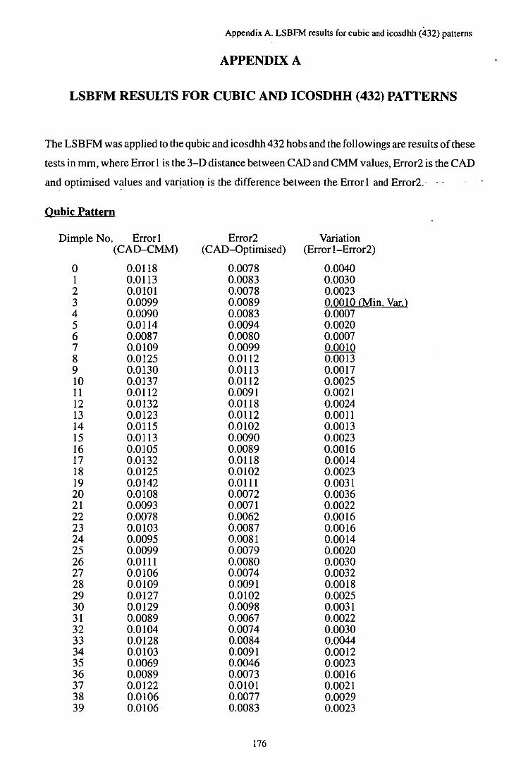
Appendix A. LSBFM results for cubic and icosdhh (432) patterns
APPENDIX A
LSBFM RESULTS FOR CUBIC AND ICOSDHH (432) PATTERNS
The LSBFM was applied to the qubic and icosdhh 432 hobs and the followings are results of these
tests in mm, where Error I is the 3-D distance between CAD and CMM values, Error2 is the CAD
and optimised values and variatioll is the difference between the Error! and Error2.
Qubic Pattern
Dimple No. Error I Error2 Variation (CAD-CMM) (CAD-Optimised) (Error I-Error2)
0 0.0118 0.0078 0.0040 I 0.0113 0.0083 0.0030 2 0.0101 0.0078 0.0023 3 0.0099 0.0089 O,QOIO (Min. Var.) 4 0.0090 0.0083 0.0007 5 0.0114 0.0094 0.0020 6 0.0087 0.0080 0.0007 7 0.0109 0.0099 0.0010 8 0.0125 0.0112 0.0013 9 0.0130 0.0113 0.0017 10 0.0137 0.0112 0.0025 11 0.0112 0.0091 0.0021 12 0.0132 0.0118 0.0024 13 0.0123 0.0112 0.0011 14 0.0115 0.0102 0.0013 15 0.0113 0.0090 0.0023 16 0.0105 0.0089 0.0016 17 0.0132 0.0118 0.0014 18 0.0125 0.0102 0.0023 19 0.0142 0.01ll 0.0031 20 0.0108 0.0072 0.0036 21 0.0093 0.0071 0.0022 22 0.0078 0.0062 0.0016 23 0.0103 0.0087 0.0016 24 0.0095 0.0081 0.0014 25 0.0099 0.0079 0.0020 26 0.0111 0.0080 0.0030 27 0.0106 0.0074 0.0032 28 0.0109 0.0091 0.0018 29 0.0127 0.0102 0.0025 30 0.0129 0.0098 0.0031 31 0.0089 0.0067 0.0022 32 0.0104 0.0074 0.0030 33 0.0128 0.0084 0.0044 34 0.0103 0.0091 0.0012 35 0.0069 0.0046 0.0023 36 0.0089 0.0073 0.0016 37 0.0122 0.0101 0.0021 38 0.0106 0.0077 0.0029 39 0.0106 0.0083 0.0023
176

Appendix A. LSBFM results for cubic and icosdhh (432) patterns
40 0.0103 0.0066 0.0037 41 0.0139 0.0101 0.0038 42 0.0149 0.0111 0.0038 43 0.0111 0.0071 0.0040 44 0.0084 0.0059 0.0025 45 0.0096 0.0063 0.0033 46 0.0102 0.0076 0.0026 47 0.0115 0.0072 0.0043 48 0.0113 0.0085 0.0028 49 0.0117 0.0099 0.00t8 50 - -0.0098 0.0075 0.0023 51 0.0048 0.0023 0.0025 52 0.0129 0.0088 0.0041 53 0.0116 0.0105 0.0011 54 0.0070 0.0057 0.0013 55 0.0106 0.0087 0.0019 56 0.0072 0.0047 0.0025 57 0.0128 0.0091 0.0037 58 0.0104 0.0084 0.0020 59 0.0059 0.0027 0.0032 60 0.0081 0.0049 0.0032 61 0.0086 0.0046 0.0040 62 0.0089 0.0051 0.0038 63 0.0107 0.0087 0.0020 64 0.0099 0.0072 0.0027 65 0.0106 0.0074 0.0032 66 0.0119 0.0090 0.0029 67 0.0098 0.0064 0.0034 68 0.0131 0.0110 0.0021 69 0.0107 0.0091 0.0016 70 0.0110 0.0083 0.0027 71 0.0098 0.0069 0.0029 72 0.0116 0.0069 0.0047 73 0.0069 0.0037 0.0032 74 0.0073 0.0041 0.0032 75 0.0112 0.0091 0.0021 76 0.0109 0.0098 0.0011 77 0.0108 0.0081 0.0027 78 0.0105 0.0082 0.0023 79 0.0118 0.0083 0.0035 80 0.0132 0.0101 0.0031 81 0.0147 0.0106 0.0041 82 0.0077 0.0042 0.0035 83 0.0114 0.0092 0.0022 84 0.0098 0.0068 0.0030 85 0.0113 0.0091 0.0022 86 0.0109 0.0084 0.0025 87 0.0106 0.0086 0.0020 88 0.0109 0.0072 0.0037 89 0.0107 0.0087 0.0020 90 0.0103 0.0079 0.0024 91 0.0108 0.0083 0.0025 92 0.0092 0.0071 0.0021 93 0.0096 0.0072 0.0024 94 0.0127 0.0097 0.0030 95 0.0103 0.0092 0.0011 96 0.0112 0.0080 0.0032 97 0.0124 0.0110 0.0014
177
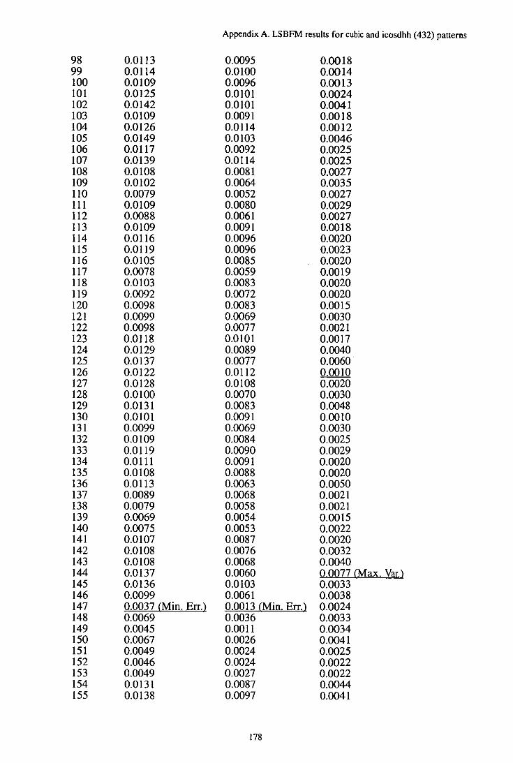
98 99 100 101 102 103 104 105 106 107 108 109 110 111 112 113 114 115 116 117 118 119 120 121 122 123 124 125 126 127 128 129 130 131 132 133 134 135 136 137 138 139 140 141 142 143 144 145 146 147 148 149 150 151 152 153 154 155
0.0113 0.0114 0.0109 0.0125 0.0142 0.0109 0.0126 0.0149 0.0117 0.0139 0.0108 0.0102 0.0079 0.0109 0.0088 0.0109 0.0116 0.0119 0.0105 0.0078 0.0103 0.0092 0.0098 0.0099 0.0098 0.01 18 0.0129 0.0137 0.0122 0.0128 0.0100 0.0131 0.0101 0.0099 0.0109 0.0119 0.0111 0.0108 0.0113 0.0089 0.0079 0.0069 0.0075 0.0107 0.0108 0.0108 0.0137 0.0136 0.0099 0.0037 (Min. Err.) 0.0069 0.0045 0.0067 0.0049 0.0046 0.0049 0.0131 0.0138
Appendix A. LSBFM results for cubic and icosdhh (432) patterns
0.0095 0.0100 0.0096 0.0101 0.0101 0.0091 0.0114 0.0103 0.0092 0.0114 0.0081 0.0064 0.0052 0.0080 0.0061 0.0091 0.0096 0.0096 0.0085 0.0059 0.0083 0.0072 0.0083 0.0069 0.0077 0.0101 0.0089 0.0077 0.0112 0.0108 0.0070 0.0083 0.0091 0.0069 0.0084 0.0090 0.0091 0.0088 0.0063 0.0068 0.0058 0.0054 0.0053 0.0087 0.0076 0.0068 0.0060 0.0103 0.0061 0.0013 (Min. Err.) 0.0036 0.0011 0.0026 0.0024 0.0024 0.0027 0.0087 0.0097
178
0.0018 0.0014 0.0013 0.0024 0.0041 0.0018 0.0012 0.0046 0.0025 0.0025 0.0027 0.0035 0.0027 0.0029 0.0027 0.0018 0.0020 0.0023 0.0020 0.0019 0.0020 0.0020 0.0015 0.0030 0.0021 0.0017 0.0040 0.0060 0.0010 0.0020 0.0030 0.0048 0.0010 0.0030 0.0025 0.0029 0.0020 0.0020 0.0050 0.0021 0.0021 0.0015 0.0022 0.0020 0.0032 0.0040 0.0077 (Max. Var.) 0.0033 0.0038 0.0024 0.0033 0.0034 0.0041 0.0025 0.0022 0.0022 0.0044 0.0041
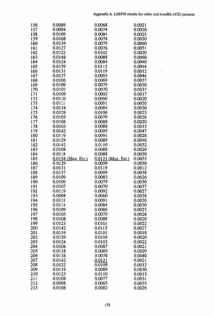
156 157 158 159 160 161 162 163 164 165 166 167 168 169 170 171 172 173 174 175 176 177 178 179 180 181 182 183 184 185 186 187 188 189 190 191 192 193 194 195 196 197 198 199 200 201 202 203 204 205 206 207 208 209 210 211 212 213
0.0089 0.0094 0.0109 0.0108 0.0139 0.0127 0.0122 0.0148 0.0124 0.0159 0.0131 0.0137 0.0106 0.0109 0.0107 0.0109 0.0110 0.0111 0.0114 0.0129 0.0105 0.0108 0.0103 0.0142 0.0119 0.0129 0.0142 0.0108 0.0118 0.0154 CMax. Err.) 0.0129 0.0131 0.0137 0.0109 0.0109 0.0107 0.0119 0.0098 0.0111 0.0114 0.0109 0.0105 0.0108 0.0123 0.0142 0.0119 0.0129 0.0124 0.0108 0.0118 0.0118 0.0142 0.0122 0.0119 0.0123 0.0108 0.0098 0.0108
Appendix A. LSBFM results for cubic and icosdhh (432) patterns
0.0068 0.0074 0.0084 0.0078 0.0079 0.0076 0.0102 0.0088 0.0084 0.0115 0.0119 0.0093 0.0069 0.0079 0.0070 0.0092 0.0090 0.0091 0.0084 0.0106 0.0079 0.0088 0.0088 0.0095 0.0091 0.0089 0.0110 0.0088 0.0088 0.0121 CMax. Err.) 0.0099 0.0119 0.0099 0.0083 0.0079 0.0070 0.0092 0.0060 0.0091 0.0084 0.0086 0.0079 0.0088 0.0101 0.0115 0.0101 0.0109 0.0102 0.0087 0.0089 0.0078 0.0121 0.0109 0.0089 0.0110 0.0077 0.0065 0.0082
179
0.0021 0.0020 0.0025 0.0030 0.0060 0.0051 0.0020 0.0060 0.0040 0.0044 0.0012 0.0044 0.0037 0.0030 0.0037 0.0017 0.0020 0.0020 0.0030 0.0023 0.0026 0.0020 0.0015 0.0047 0.0028 0.0040 0.0032 0.0020 0.0030 0.0033 0.0030 0.0012 0.0038 0.0026 0.0030 0.0037 0.0027 0.0038 0.0020 0.0030 0.0023 0.0026 0.0020 0.0022 0.0027 0.0018 0.0020 0.0022 0.0021 0.0029 0.0040 0.0021 0.0013 0.0030 0.0013 0.0031 0.0033 0.0026
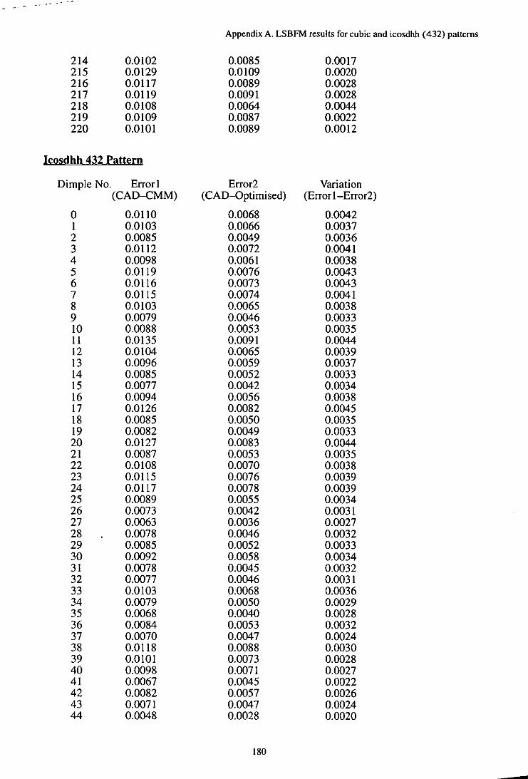
Appendix A. LSBFM results for cubic and icosdhh (432) patterns
214 0.0102 0.0085 0.0017 215 0.0129 0.0109 0.0020 216 0.0117 0.0089 0.0028 217 0.0119 0.0091 0.0028 218 0.0108 0.0064 0.0044 219 0.0109 0.0087 0.0022 220 0.0101 0.0089 0.0012
Icosdhh 432 Pattern
Dimple No. Error 1 Error2 Variation (CAD-CMM) (CAD-Optimised) (Error 1-Error2)
0 0.0110 0.0068 0.0042 1 0.0103 0.0066 0.0037 2 0.0085 0.0049 0.0036 3 0.0112 0.0072 0.0041 4 0.0098 0.0061 0.0038 5 0.0119 0.0076 0.0043 6 0.0116 0.0073 0.0043 7 0.0115 0.0074 0.0041 8 0.0103 0.0065 0.0038 9 0.0079 0.0046 0.0033 10 0.0088 0.0053 0.0035 11 0.0135 0.0091 0.0044 12 0.0104 0.0065 0.0039 13 0.0096 0.0059 0.0037 14 0.0085 0.0052 0.0033 15 0.0077 0.0042 0.0034 16 0.0094 0.0056 0.0038 17 0.0126 0.0082 0.0045 18 0.0085 0.0050 0.0035 19 0.0082 0.0049 0.0033 20 0.0127 0.0083 0.0044 21 0.0087 0.0053 0.0035 22 0.0108 0.0070 0.0038 23 0.0115 0.0076 0.0039 24 0.0117 0.0078 0.0039 25 0.0089 0.0055 0.0034 26 0.0073 0.0042 0.0031 27 0.0063 0.0036 0.0027 28 0.0078 0.0046 0.0032 29 0.0085 0.0052 0.0033 30 0.0092 0.0058 0.0034 31 0.0078 0.0045 0.0032 32 0.0077 0.0046 0.0031 33 0.0103 0.0068 0.0036 34 0.0079 0.0050 0.0029 35 0.0068 0.0040 0.0028 36 0.0084 0.0053 0.0032 37 0.0070 0.0047 0.0024 38 0.0118 0.0088 0.0030 39 0.0101 0.0073 0.0028 40 0.0098 0.0071 0.0027 41 0.0067 0.0045 0.0022 42 0.0082 0.0057 0.0026 43 0.0071 0.0047 0.0024 44 0.0048 0.0028 0.0020
180
-
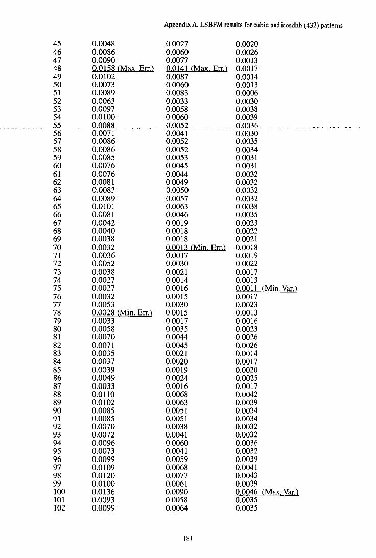
Appendix A. LSBFM results for cubic and icosdbb (432) patterns
45 0.0048 0.0027 0.0020 46 0.0086 0.0060 0.0026 47 0.0090 0.0077 0.0013 48 0.0158 (Max. Err.} Q Ql~l (Max. Err.} 0.0017 49 0.0102 0.0087 0.0014 50 0.0073 0.0060 0.0013 51 0.0089 0.0083 0.0006 52 0.0063 0.0033 0.0030 53 0.0097 0.0058 0.0038 54 0.0100 0.0060 0.0039 55 . _--- ----- 0.0088 . 0.0052 .. ._ . _ ... 0.0036 . . . . - .. - - - - - .
56 0.0071 0.0041 0.0030 57 0.0086 0.0052 0.0035 58 0.0086 0.0052 0.0034 59 0.0085 0.0053 0.0031 60 0.0076 0.0045 0.0031 61 0.0076 0.0044 0.0032 62 0.0081 0.0049 0.0032 63 0.0083 0.0050 0.0032 64 0.0089 0.0057 0.0032 65 0.0101 0.0063 0.0038 66 0.0081 0.0046 0.0035 67 0.0042 0.0019 0.0023 68 0.0040 0.0018 0.0022 69 0.0038 0.0018 0.0021 70 0.0032 Q QQJ 3 (Min. Err.} 0.0018 71 0.0036· 0.0017 0.0019 12 0.0052 0.0030 0.0022 73 0.0038 0.0021 0.0017 74 0.0027 0.0014 0.0013 75 0.0027 0.0016 Q.QQ11 (Min. Var.} 76 0.0032 0.0015 0.0017 77 0.0053 0.0030 0.0023 78 0.0028 (Min. Err.} 0.0015 0.0013 79 0.0033 0.0017 0.0016 80 0.0058 0.0035 0.0023 81 0.0070 0.0044 0.0026 82 0.0071 0.0045 0.0026 83 0.0035 0.0021 0.0014 84 0.0037 0.0020 0.0017 85 0.0039 0.0019 0.0020 86 0.0049 0.0024 0.0025 87 0.0033 0.0016 0.0017 88 0.0110 0.0068 0.0042 89 0.0102 0.0063 0.0039 90 0.0085 0.0051 0.0034 91 0.0085 0.0051 0.0034 92 0.0070 0.0038 0.0032 93 0.0012 0.0041 0.0032 94 0.0096 0.0060 0.0036 95 0.0073 0.0041 0.0032 96 0.0099 0.0059 0.0039 97 0.0109 0.0068 0.0041 98 0.0120 0.0077 0.0043 99 0.0100 0.0061 0.0039 100 0.0136 0.0090 0.0046 (Max. Var.} 101 0.0093 0.0058 0.0035 102 0.0099 0.0064 0.0035
181
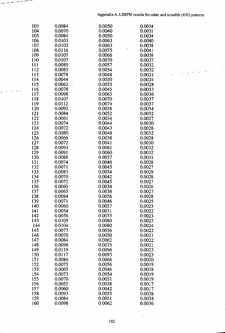
--~------
103 104 105 106 107 108 109 110 111 112 113 114 115 116 117 118 119 120 121 122 123 124 125 126 127 128 129 130 131 132 133 134 135 136 137 138 139 140 141 142 143 144
145 146 147 148 149 150 . 151 152 153 154 155 156 157 158 159 160
0.0084 0.0070 0.0084 0.0103 0.0102 0.0116 0.0105 0.0107 0.0089 0.0085 0.0078 0.0044 0.0062 0.0078 0.0098 0.0107 0.0112 0.0092 0.0084 0.0061 0.0074 0.0072 0.0080 0.0066 0.0072 0.0093 0.0091 0.0088 0.0074 0.0071 0.0083 0.0070 0.0072 0.0060 0.0065 0.0084 0.0071 0.0060 0.0054 0.0056 0.0105 0.0104 0.0077 0.0070 0.0084 0.0096 0.0119 0.0117 0.0086 0.0075 0.0065 0.0073 0.0070 0.0055 0.0060 0.0093 0.0084 0.0098
Appendix A. LSBFM results for cubic and icosdhh (432) patterns
0.0050 0.0040 0.0050 0.0063 0.0063 0.0075 0.0066 0.0070 0.0057 0.0054 0.0048 0.0020 0.0035 0.0045 0.0063 0.0070 0.0074 0.0058 0.0052 0.0034 0.0044 0.0043 0.0048 0.0038 0.0041 0.0061 0.0060 0.0057 0.0046 0.0045 0.0054 0.0042 0.0045 0.0034 0.0038 0.0056 0.0046 0.0037 0.0031 0.0033 0.0080 0.0080 0.0056 0.0050 0.0062 0.0075 0.0096 0.0093 0.0066 0.0056 0.0046 0.0054 0.0051 0.0038 0.0042 0.0055 0.0051 0.0062
182
0.0034 0.0031 0.0034 0.0040 0.0038 0.0041 0.0038 0.0037 0.0032 0.0032 0.0031 0.0024 0.0028 0.0033 0.0036 0.0037 0.0037 0.0034 0.0032 0.0027 0.0030 0.0028 0.0032 0.0028 0.0030 0.0032 0.0032 0.0031 0.0028 0.0027 0.0029 0.0028 0.0027 0.0026 0.0027 0.0028 0.0025 0.0023 0.0022 0.0023 0.0025 0.0024 0.0022 0.0021 0.0022 0.0021 0.0023 0.0023 0.0020 0.0019 0.0018 0.0019 0.0019 0.0017 0.0017 0.0038 0.0034 0.0036
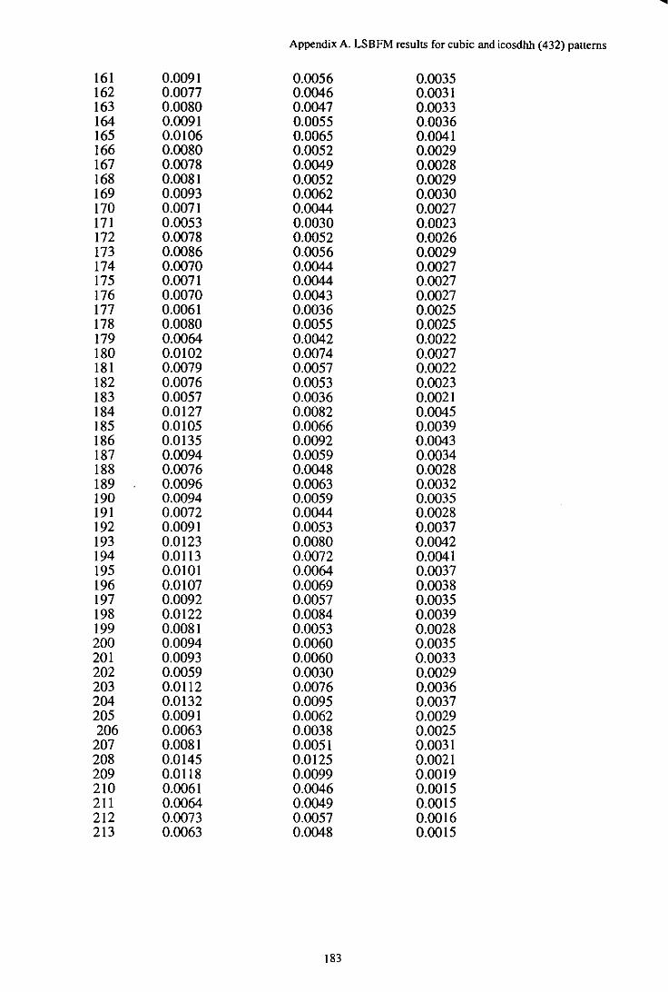
Appendix A. LSBFM results for cubic and icosdhh (432) patterns
161 0.0091 0.0056 0.0035 162 0.0077 0.0046 0.0031 163 0.0080 0.0047 0.0033 164 0.0091 0.0055 0.0036 165 0.0106 0.0065 0.0041 166 0.0080 0.0052 0.0029 167 0.0078 0.0049 0.0028 168 0.0081 0.0052 0.0029 169 0.0093 0.0062 0.0030 170 0.0071 0.0044 0.0027 171 0.0053 0.0030 0.0023 172 0.0078 0.0052 0.0026 173 0.0086 0.0056 0.0029 174 0.0070 0.0044 0.0027 175 0.0071 0.0044 0.0027 176 0.0070 0.0043 0.0027 177 0.0061 0.0036 0.0025 178 0.0080 0.0055 0.0025 179 0.0064 0.0042 0.0022 180 0.0102 0.0074 0.0027 181 0.0079 0.0057 0.0022 182 0.0076 0.0053 0.0023 183 0.0057 0.0036 0.0021 184 0.0127 0.0082 0.0045 185 0.0105 0.0066 0.0039 186 0.0135 0.0092 0.0043 187 0.0094 0.0059 0.0034 188 0.0076 0.0048 0.0028 189 0.0096 0.0063 0.0032 190 0.0094 0.0059 0.0035 191 0.0072 0.0044 0.0028 192 0.0091 0.0053 0.0037 193 0.0123 0.0080 0.0042 194 0.0113 0.0072 0.0041 195 0.0101 0.0064 0.0037 196 0.0107 0.0069 0.0038 197 0.0092 0.0057 0.0035 198 0.0122 0.0084 0.0039 199 0.0081 0.0053 0.0028 200 0.0094 0.0060 0.0035 201 0.0093 0.0060 0.0033 202 0.0059 0.0030 0.0029 203 0.0112 0.0076 0.0036 204 0.0132 0.0095 0.0037 205 0.0091 0.0062 0.0029 206 0.0063 0.0038 0.0025 207 0.0081 0.0051 0.0031 208 0.0145 0.0125 0.0021 209 0.0118 0.0099 0.0019 210 0.0061 0.0046 0.0015 211 0.0064 0.0049 0.0015 212 0.0073 0.0057 0.0016 213 0.0063 0.0048 0.0015
183
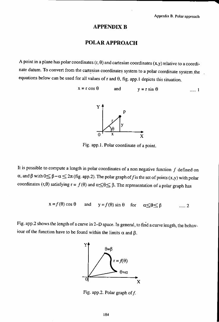
Appendix B. Polar approach
APPENDIXB
POLAR APPROACH
A point in a plane has polar coordinates (r, 6) and cartesian coordinates (x,y) relative to a coordi
nate datum. To convert from the cart~sian coordinates system to a polar coordinate system. the
equations below can be used for all values of r and 6, fig. app.l depicts this situation.
x=rcos6 and y = r sin 6 ..... I
y p
y
o x
Fig. app.l. Polar coordinate of a point.
It is possible to compute a length in polar coordinates of a non negative function 1 defined on
a, and ~ with 0< ~-a< 21t (fig. app.2). The polar graph of lis the set of points (x,y) with polar
coordinates (r,6) satisfying r = 1 (6) and a<6< ~. The representation of a polar graph has
x = 1(6) cos 6 and y = 1 (6) sin 6 for a<6< ~ ..... 2
Fig. app.2 shows the length of a curve in 2-D space. In general, to find a curve length, the behav
iour of the function have to be found within the limits a and ~.
y
r = 1(6)
6=a
o x
Fig. app.2. Polar graph off
184
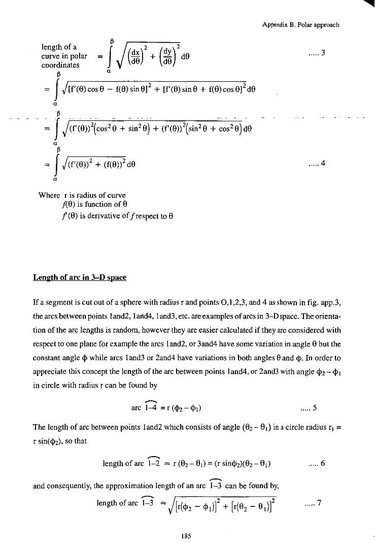
Appendix B. Polar approach
~ length of a f curve in polar = coordinates
~ a
= f j[f'(8)cos8 - f(8) sin 8]2 + [f'(8)sin8 + f(8)cos8]2d8
a
~ j (f'(8»2( cos2 8 + sin2 8) + (f'(8»2( sin2 8 + cos2 8) d8
a ~
= f j(£'(8»2 + (f(8»2 d8
a
Where r is radius of curve !(8) is function of 8
f(8) is derivative ofjrespect to 8
Length of arc in 3-D space
..... 3
..... 4
If a segment is cut out of a sphere with radius r and points 0,1,2,3, and 4 as shown in fig. app.3,
the arcs between points I and2, I and4, I and3, etc. are examples of arcs in 3-D space. The orienta
tion of the arc lengths is random, however they are easier calculated if they are considered with
respect to one plane for example the arcs land2, or 3and4 have some variation in angle 8 but the
constant angle <I> while arcs land3 or 2and4 have variations in both angles e and <1>. In order to
appreciate this concept the length of the arc between points land4, or 2and3 with angle <1>2 - <1>,
in circle with radius r can be found by
.---. arc 1-4 = r (<1>2 - <1>,) ..... 5
The length of arc between points land2 which consists of angle (82 - 8d in a circle radius r, =
r sine <1>2), so that
.---. length of arc 1-2 = r (82 - 8,) = (r sin<l>2)(8z - 8,) ..... 6
.---. and consequently, the approximation length of an arc 1-3 can be found by,
length of arc 1-3 = j[r(<I>2 - <1>1)]2 + [r(82 _ 81)]2 ..... 7
185
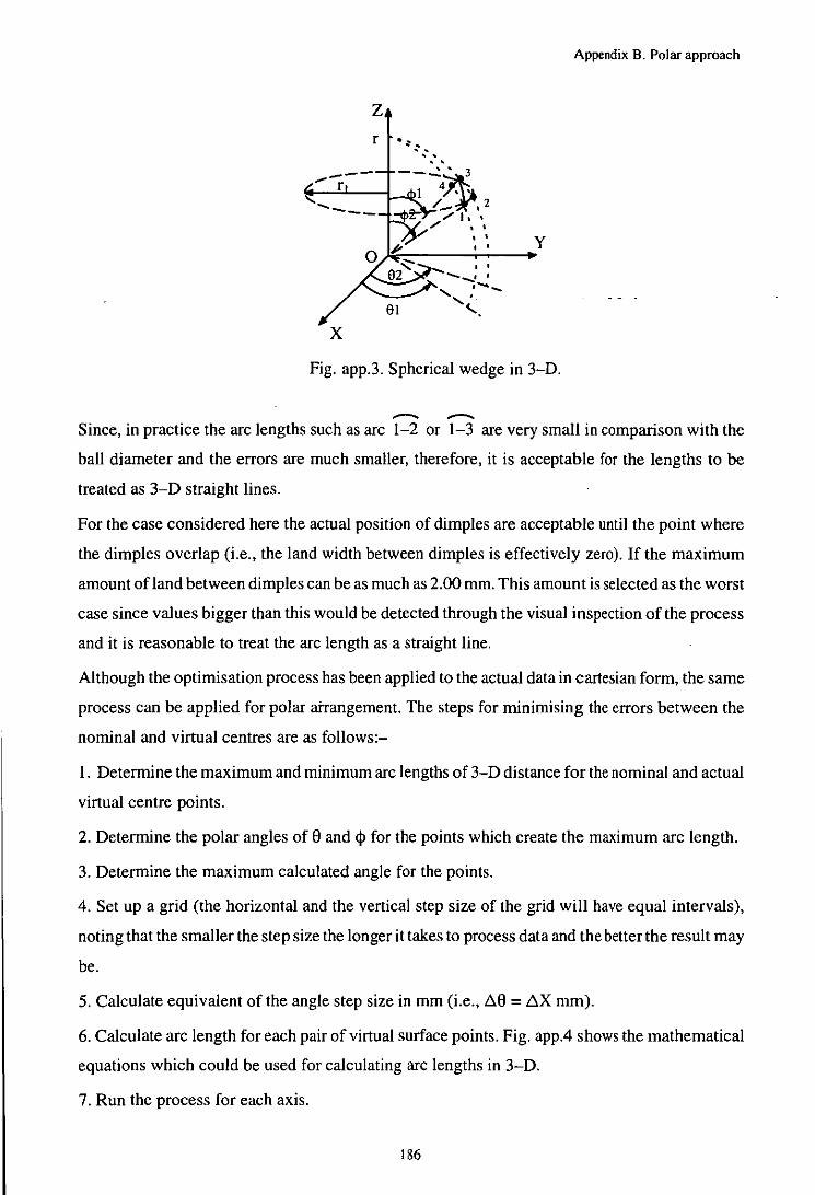
x
z r
, , " y
~~----~'~'---+ - " --....:o:=--" ............. ! I .-',' 91 '. Fig. app.3. Spherical wedge in 3-D .
..---. ..---.
Appendix B. Polar approach
Since, in practice the arc lengths such as arc 1-2 or 1-3 are very small in comparison with the
ball diameter and the errors are much smaller, therefore, it is acceptable for the lengths to be
treated as 3-D straight lines.
For the case considered here the actual position of dimples are acceptable until the point where
the dimples overlap (i.e., the land width between dimples is effectively zero). If the maximum
amount of land between dimples can be as much as 2.00 mm. This amount is selected as the worst
case since values bigger than this would be detected through the visual inspection of the process
and it is reasonable to treat the arc length as a straight line.
Although the optimisation process has been applied to the actual data in cartesian form, the same
process can be applied for polar arrangement. The steps for minimising the errors between the
nominal and virtual centres are as follows:-
I. Determine the maximum and minimum arc lengths of 3-D distance for the nominal and actual
virtual centre points.
2. Determine the polar angles of 8 and <I> for the points which create the maximum arc length.
3. Determine the maximum calculated angle for the points.
4. Set up a grid (the horizontal and the vertical step size of the grid will have equal intervals),
noting that the smaller the step size the longer it takes to process data and the better the result may
be.
5. Calculate equivalent of the angle step size in mm (i.e., ~8 = ~X mm).
6. Calculate arc length for each pair of virtual surface points. Fig. app.4 shows the mathematical
equations which could be used for calculating arc lengths in 3-D.
7. Run the process for each axis.
186
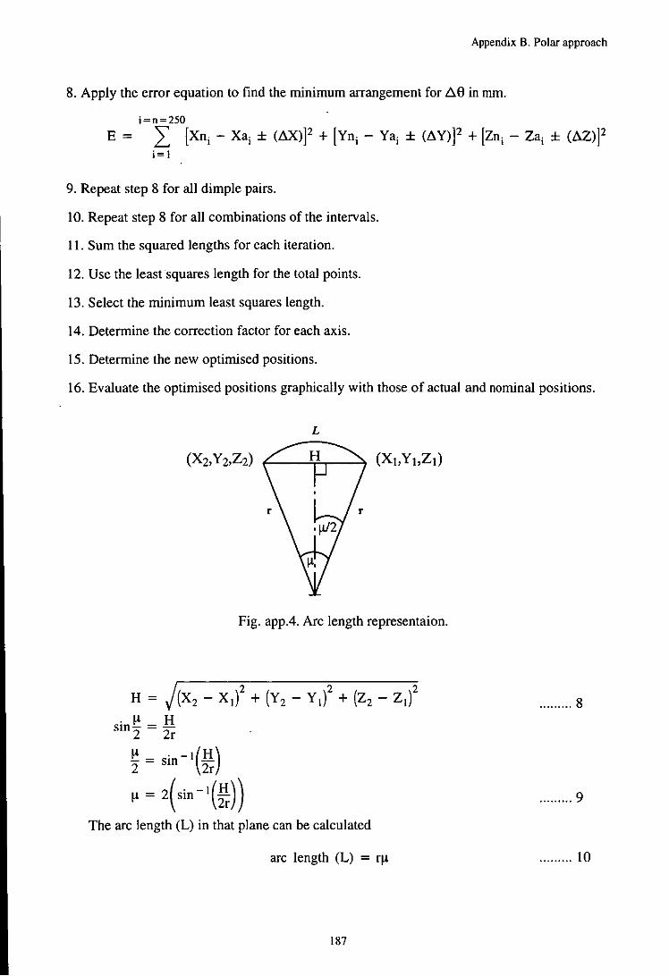
Appendix B. Polar approach
8. Apply the error equation to find the minimum arrangement for Li.8 in nun.
j=n=250
E = I [Xnj - Xaj ± C6X)j2 + [Ynj - Yaj ± CL\YW + [Znj - Zaj ± CL\z)j2 j=1
9. Repeat step 8 for all dimple pairs.
10. Repeat step 8 for all combinations of the intervals.
11. Sum the squared lengths for each iteration.
12. Use the least squares length for the total points.
13. Select the minimum least squares length.
14. Determine the correction factor for each axis.
15. Determine the new optimised positions.
16. Evaluate the optimised positions graphically with those of actual and nominal positions.
L
Fig. app.4. Arc length representaion.
. ........ 8
......... 9
The arc length CL) in that plane can be calculated
arc length CL) = rlt ......... 10
187
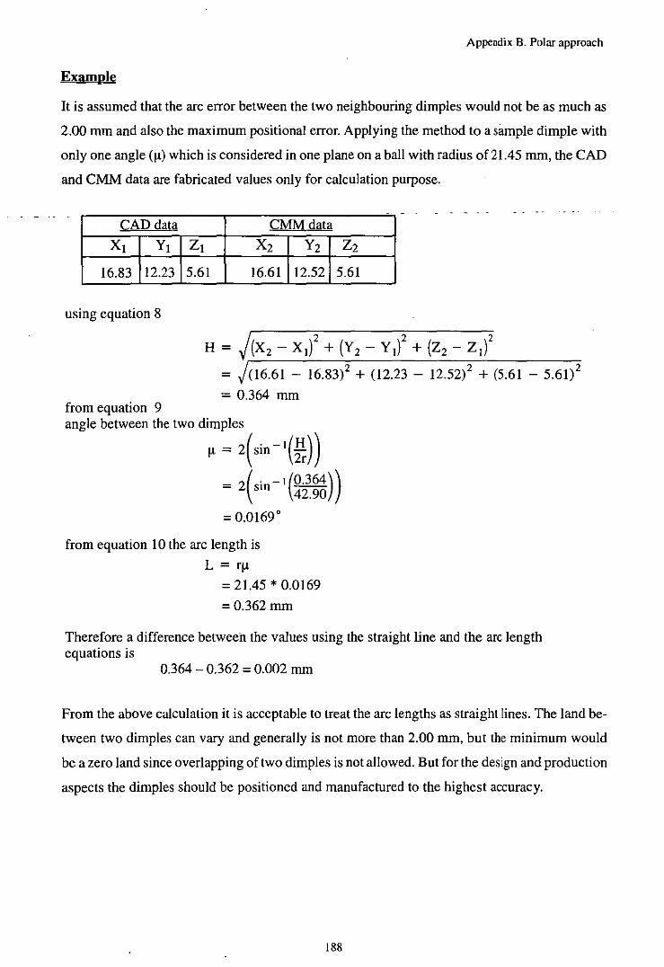
Appendix B. Polar approach
Example
It is assumed that the arc error between the two neighbouring dimples would not be as much as
2.00 mm and also the maximum positional error. Applying the method to a sample dimple with
only one angle (11) which is considered in one plane on a ball with radius of 21.45 mm, the CAD
and CMM data are fabricated values only for calculation purpose.
CAD data CMMdata
Xl YI Zl X2 Y2 Z2
16.83 12.23 5.61 16.61 12.52 5.61
using equation 8
= 0.364 mm from equation 9 angle between the two dimples
11 = 2(sin-I(~)) = 2(sin -1 (0.364))
42.90
= 0.0169°
from equation 10 the arc length is
L = rll
= 21.45 * 0.0169
= 0.362 mm
Therefore a difference between the values using the straight line and the arc length equations is
0.364 - 0.362 = 0.002 mm
From the above calculation it is acceptable to treat the arc lengths as straight lines. The land be
tween two dimples can vary and generally is not more than 2.00 mm, but the minimum would
be a zero land since overlapping of two dimples is not allowed. But forthe design and production
aspects the dimples should be positioned and manufactured to the highest accuracy.
188