1.1 INTEGRATED LEARNING IN MULTI-NET SYSTEMS........................................................................10 1.2 STRUCTURE OF THIS THESIS..........................................................................................................13
2 SINGLE-NET AND MULTI-NET SYSTEMS.............................................................................15
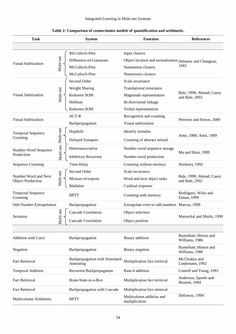
2.1 SINGLE-NET SYSTEMS: LEARNING PARADIGMS AND TECHNIQUES.............................................16 2.2 MULTI-NET SYSTEMS: CATEGORISATION AND COMBINATION STRATEGIES...............................25 2.3 NUMERICAL PROCESSING: PSYCHOLOGICAL AND PHYSIOLOGICAL EVIDENCE ..........................45 2.4 SIMULATING NUMERICAL ABILITIES WITH NEURAL NETWORKS ................................................52 2.5 SUMMARY......................................................................................................................................62
3 IN-SITU LEARNING IN MULTI-NET SYSTEMS....................................................................65
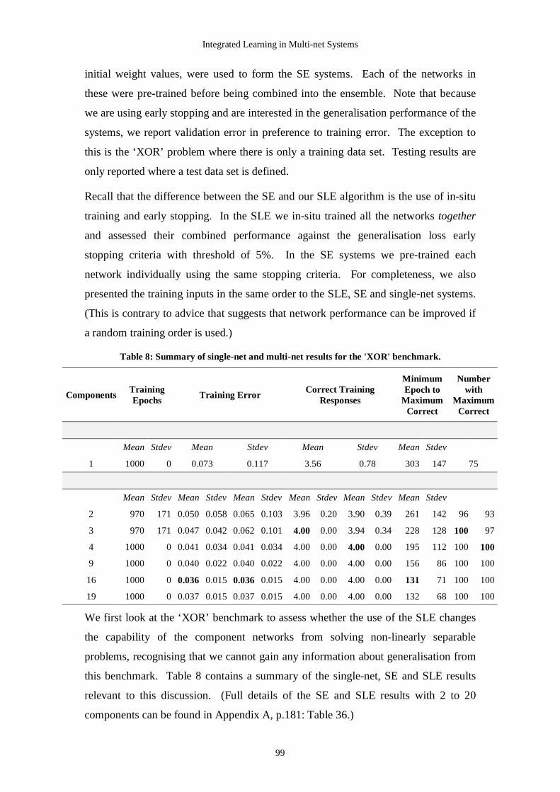
3.1 A FRAMEWORK FOR MULTI-NET SYSTEMS..................................................................................69 3.2 IN-SITU LEARNING IN MULTI-NET SYSTEMS ................................................................................86 3.3 IN-SITU LEARNING AND BENCHMARK CLASSIFICATION ..............................................................94 3.4 SUMMARY....................................................................................................................................110
4 SIMULATING NUMERICAL ABIL ITIES WITH IN-SITU LEARNING ...........................115
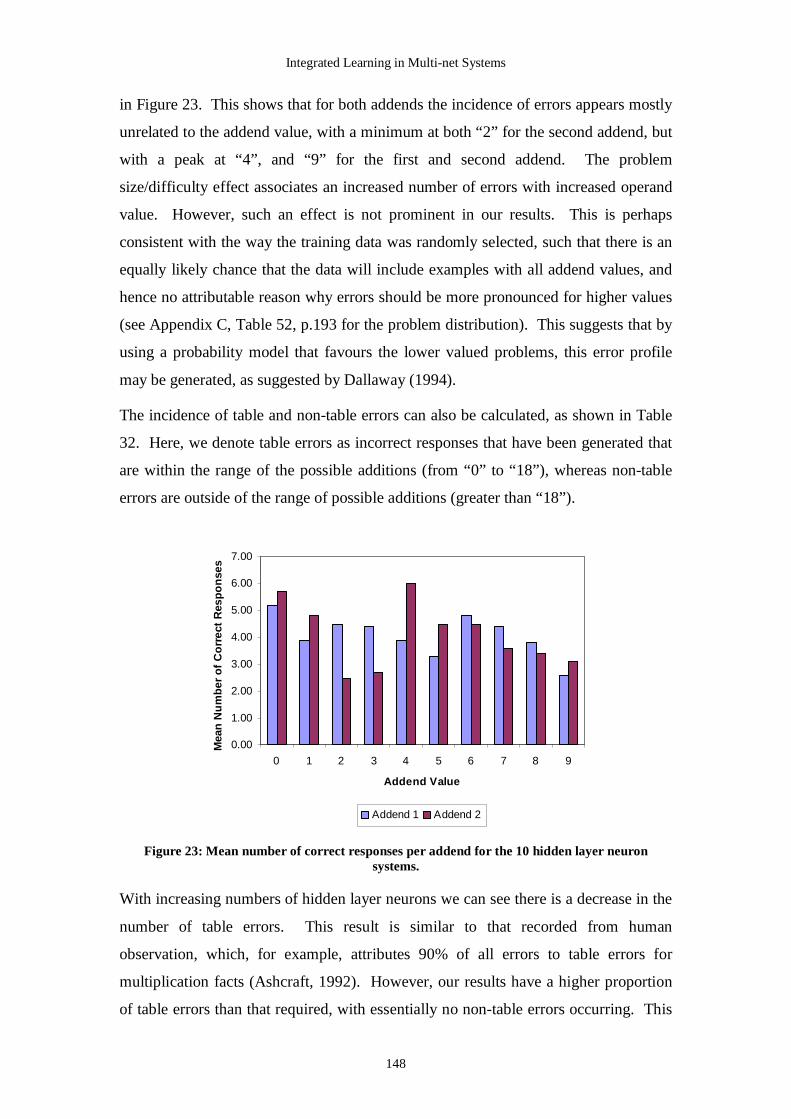
4.1 MAGNITUDE AND SYMBOLIC REPRESENTATIONS OF NUMBER..................................................119 4.2 SIMULATING QUANTIFICATION...................................................................................................125 4.3 SIMULATING ADDITION...............................................................................................................140 4.4 SUMMARY....................................................................................................................................155
5 CONCLUSION AND FUTURE WORK .....................................................................................159
5.1 CONCLUSION ...............................................................................................................................160 5.2 FUTURE WORK ............................................................................................................................164
APPENDIX A SIMPLE LEARNING ENSEMBLE RESULTS...............................................181
APPENDIX B DISTRIBUTION OF NUMBER OF OBJECTS IN DATA SETS.................187
APPENDIX C ADDITION PROBLEM DATA SETS...............................................................193
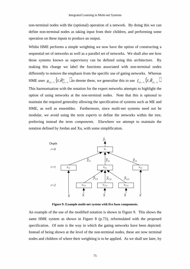
Integrated Learning in Multi-net Systems
9
1 Introduction
The construction of intelligent systems is an important topic within computer science.
It appears that one of the key features of such intelligent systems is the ability to adapt
to their experiences, a process often identified as learning. The Oxford English
Dictionary defines learning as the “process which leads to the modification of
behaviour” (Simpson and Weiner, 1989). For us, learning in artificial systems is
exemplified by connectionism, where changes in behaviour are achieved by
modifying connection strengths in a collection of interacting artificial neurons. Here
the connectionist approach relies upon our understanding of how learning is thought
to occur in biological systems, modelled in an artificial neural network.
Artificial neural networks are mathematical models of biological neuronal systems.
Here, collections of artificial neurons are taught to organise and recognise patterns
according to defined criteria, allowing them to be used for tasks such as classification,
regression and data mining. However, whilst such systems provide us with an
abstract notion of learning, it is not clear how these simple mathematical techniques
can be used to build intelligent systems. Indeed, even if we were able to build such
systems and assess their capabilities against definitions of ‘ thinking’ such as in
Turing’s (1950) imitation game, we do not yet understand how ‘ thinking’ results from
biological neurons.
Investigations into the biological basis of behaviour have noted that in humans and
non-human animals specific areas of the brain can be identified with particular
cognitive abilities. This notion of functional specialism also appears important within
artificial systems, through the decomposition of tasks to be processed by modules.
Here then we see that biological concepts, such as learning in collaboration with
modularisation, may help build artificially intelligent systems.
From a connectionist perspective, modular systems can be constructed by using
multiple neural networks. These multi-net systems have been used in different
configurations because of their statistical properties. For example, the parallel
combination of networks performing the same (non-modular) task has been shown to
improve generalisation performance, the goal of learning systems. Modular multi-net
systems have also demonstrated such capability, with some limited results. However,
a consistent and formal view of multi-net systems has yet to be provided, and this may
Integrated Learning in Multi-net Systems
10
help explore the general properties of multi-net systems, such as efficacy of modular
systems.
Within this thesis we attempt to bring together the ideas of learning taken from
biology, proposing two multi-net systems that exploit in-situ learning. To assist in the
definition of multi-net systems we provide a generalised formal framework and
learning algorithm. By way of application we return to biology, and specifically the
biological basis of behaviour, by simulating certain cognitive abilities using modular
multi-net systems that employ in-situ learning.
1.1 Integrated Learning in Multi-net Systems
The development of neural networks has lead from the construction of single neuronal
models through to the construction of multi-layered single-net systems, which can be
trained to solve wider types of problem. More recently, the properties of multi-net
systems have been seen as important, providing improved solutions to those of single
network systems under a range of conditions, either through collaboration of
networks, or competition between networks. Whilst the motivation to combine
networks is perhaps based upon their statistical properties, we can see how this may
parallel our knowledge of functional specialism in biological neural systems, despite
the apparent divide between these two disciplines.
The divergence between biology and artificial neural computing can perhaps be traced
back to Hebb’s (1949) oft cited examination of perceptual learning in the vision
system of humans and non-human animals. His neurophysiological postulate has
formed an important foundation for artificial systems, with its simple learning scheme
adopted by a number of popular neural network algorithms, and its properties
examined and subsequently enhanced. However, whilst this has seen widespread use,
little of his complementary work on combined learning across (what would now be
termed) multiple neural networks has been examined. It should be noted that Hebb
admitted that his speculation about how humans and other animals learn to integrate
single visual stimuli into perceiving more complex visual structures is ‘ far from the
actual known facts’ (1949:91). With the interest now being shown in combining
artificial neural networks, the question here is whether we can capitalise on this
biological perspective? Here we are motivated by Hebb’s ideas of ‘ superordinate’
systems: systems that are more capable than the sum of their components.
Integrated Learning in Multi-net Systems
11
In order to shed some light on this, we must first examine the theory surrounding the
combination of multiple neural networks. Multi-net systems have developed from the
statistical combination of networks to improve generalisation. Typically these
ensemble systems are formed from redundant sets of networks that perform the same
task. A similar statistical motivation has lead to the development of modular multi-
net systems where networks performing a different task are combined to improve
generalisation.
Multi-net systems have also been developed through the study of cognitive processes,
where multi-net systems have been used to simulate certain abilities. For these
simulations, networks are combined to explore psychological models that are thought
to be composed of several stages of processing. These multi-net systems therefore
rely upon prior knowledge, and do not necessarily conform to any generalised multi-
net system.
Whilst there have been a number of attempts to classify the different types of multi-
net system in use, there is no generalised way of formally specifying multi-net
systems. Not only could this help to unify the different types of multi-net models, but
this could also help explore their general properties.
Multi-net systems also employ different approaches to learning. For example,
traditional ensemble systems pre-train networks before combining them together.
More recently incremental learning techniques have been used, where individually
trained networks are combined iteratively until a desired level of performance is
achieved. The last technique is that of in-situ learning, where networks are combined
prior to training with the learning algorithm operating on this combined system. This
last form of training seems to fit well with Hebb’s ideas on ‘neural integration’
(1949:84), where he proposed that not only do cell assemblies learn through a process
of association, but also that multiple cell assemblies learn to operate together through
association. Here then, to model cognitive processes with multi-net systems, in-situ
learning would appear to be appropriate. Furthermore, this raises the question as to
whether in-situ learning would also be appropriate for the more general class of multi-
net system.
This thesis is attempting to bring together the threads discussed here by exploring the
use of in-situ learning in multi-net systems, as motivated by the theoretical
Integrated Learning in Multi-net Systems
12
development of neural networks, together with the biological basis of behaviour. We
examine in-situ learning from three different perspectives. First we build upon the
artificial domain by providing a formal framework in which multi-net systems can be
specified, including the definition of a multi-net learning algorithm. The framework
and algorithm are intended to provide a way in which general multi-net systems can
be specified. Here it is also recognised that formalising systems is an important step
towards a better understanding of their properties, helping with a rigorous analysis of
their properties.
Second we define two novel in-situ learning multi-net systems, one based upon
ensemble systems and one on modular systems. Ensemble systems are perhaps the
most popular multi-net architectures used currently, with, for example, Freund and
Schapire’s (1996) AdaBoost algorithm and variants in widespread use. Here we take
a simplified approach by examining how in-situ learning can improve ensemble
combination in a simple ensemble, one where the average of the outputs from all the
components is used. Our algorithm relies upon early stopping techniques to capitalise
on in-situ learning to generate improved solutions.
Next, we examine how in-situ learning can be used in sequential systems, and
explicitly how the simple combination of unsupervised and supervised learning can be
achieved to generate systems that are capable of solving a limited set of non-linearly
separable problems. Here we explore Hebb’s concept of superordinate integration by
attempting to sequentially combine networks into a system that is capable of solving
problems that cannot be solved by the component networks individually. To achieve
this we use the sequential combination of a Kohonen self-organising map (Kohonen,
1982) and a single layer network to solve non-linearly separable problems.
Last we return to the cognitive science domain by applying in-situ learning in multi-
net systems to simulate certain cognitive abilities, describing them using the
framework provided. The numerical abilities are examined, dealing explicitly with
quantification using subitization and counting, and addition using fact retrieval and
counting. We build upon single-net simulations of individual abilities to explore how
they interact and integrate through a process of learning in multi-net simulations.
These three different perspectives take us from the world of the artificial neuron back
Integrated Learning in Multi-net Systems
13
to the domain of the biological neuron, following the link between these two areas of
research1.
1.2 Structure of this Thesis
We have detailed above three themes that run through the concept of in-situ learning,
which are consequently reflected in the structure of this document. The main theme is
that of the development of multi-net systems, providing a background on the artificial
neural network domain and existing multi-net systems. Next is the theoretical
specification of multi-net systems, attempting to provide a foundation upon which
they can be described and then used to explore their general properties. Last, we have
the theme of behaviour, and specifically the psychology of the numerical abilities
within humans and other animals. These three themes run in parallel throughout this
thesis.
In chapter 2 we provide the traditional review of the domains discussed in this
document, covering artificial neural networks from single-net systems to multi-net
systems. Here we examine how and why multi-net systems have developed with a
summary of the current literature and problem areas. In this chapter we also explore
the psychology of the numerical abilities with a brief review of the theory and issues
surrounding current work. We relate this to the different single-net and multi-net
simulations of such abilities to provide a comparison to the work carried out in later
chapters.
In chapter 3 we present a formal framework for specifying multi-net systems, together
with a learning algorithm. With this we provide a generalised way in which multi-net
systems can be defined. This is related to the current multi-net literature with a
number of examples. Moving forward from this we use the framework to define two
in-situ learning multi-net systems, one based upon existing ensemble techniques, and
one exploring sequential learning. To conclude this chapter we present a benchmark
evaluation of both algorithms, comparing their performance with existing single-net
and multi-net techniques, demonstrating that they can be used to improve
1 This seems to fit well with current initiatives, such as the Grand Challenges for Computer Science (Hoare et al, 2003) Architecture of Brain and Mind proposal (Denham, 2002), and the Foresight Cognitive Systems Project (Foresight Directorate, 2002).
Integrated Learning in Multi-net Systems
14
generalisation performance as compared with single-net and other multi-net
techniques.
In chapter 4 we shift back to the theme of biology with the biological basis of
behaviour. Here we apply in-situ learning to explore simulations of the interaction
between specific cognitive abilities. We start with exploring quantification, providing
single-net simulations of subitization and counting, before combining these into a
multi-net simulation of quantification, comparing the results with existing simulations
of the quantification abilities. Next we look at addition by simulating the fact
retrieval and ‘count all’ strategies, before again combining these into a multi-net
simulation of addition. We conclude that in-situ learning in modular systems offers
an alternative view of how such abilities can give rise to observed phenomena, such as
the subitization limit.
In chapter 5 we summarise the work presented and look forward to how this work can
be developed in the future.
Integrated Learning in Multi-net Systems
15
2 Single-net and Multi-net Systems
Artificial neural networks (ANNs) are mathematical models of networks of biological
neurons. The elementary artificial neuron constructed by modelling biology forms a
greatly simplified view of the neurophysiological processes found within the brains of
animals and humans. Elements such as connection strength (excitatory or inhibitory),
connection combination and activation threshold are present in these models of
biological neurons, in which learning is achieved through the modification of
connection weights in response to an input stimulus.
According to Hebb learning occurs when ‘some growth process or metabolic change
takes place’ (1949:62). Learning in ANNs is typically achieved through the
application of an algorithm that modifies the connection weights in response to an
input stimulus, making them more excitatory or inhibitory. This plasticity in
connection weight values is a powerful mechanism that provides neural networks with
the ability to adapt to their input and to produce outputs that can be tailored for a
variety of problems, including classification and regression. Furthermore, training is
achieved through modification of network parameters (weights) alone and not the
network architecture (neurons).
The goal of this learning process is to generate a system that can generalise: the
ability to recognise patterns in novel inputs on which a network has not been trained.
Generalisation in ANNs allows them to be applied to those problems for which a
complete definition of the input space is not possible, or indeed practical, but from
which a suitable set of similar values and responses can be defined through a learning
process. Both learning and generalisation are the key elements that make neural
networks useful, yet they only become practical when individual neurons can be
combined together into networks, allowing them to be applied to solve complex
problems with multiple layers of activity, modelling (albeit on a very small scale) the
connectivity of the brain.
Such multi-neuron, parallel distributed processing (PDP) systems (McClelland and
Rumelhart, 1986) demonstrate the importance of how individual processing units may
be combined in a neural network, or single-nets in the context of this thesis.
However, successfully applying neural networks to a problem relies upon suitable
choices of network topology, learning algorithm, parameters and training data. These
Integrated Learning in Multi-net Systems
16
choices are typically based upon prior knowledge coupled with experimentation, with
a balance between the application of prior knowledge and algorithmic changes
required to avoid over or under training and hence potentially poor generalisation.
Improvements in these aspects of ANNs leads to the development of algorithms and
architectures that can demonstrate increased learning speeds and robust generalisation
capabilities.
The combination of neurons into networks demonstrates how simple processing
elements may be combined into systems that are capable of processing complex
problems, learning from examples as a coherent system. What is of interest to us is
the combination of such single-net systems into multi-net systems, exploring whether
a similar approach to learning, where both the networks and their combination learn
in-situ, shows any improvement over the combination of pre-trained networks. With
this in mind in this chapter a selection of single-net architectures and learning
algorithms is presented, followed by a review of the development of these systems
into multi-net architectures, concentrating on those aspects that are important in the
development and formulation of multi-net systems and looking at the ways in which
components can be combined. Lastly, in this chapter we look at multi-net systems
within the context of cognitive science, which lends itself well to exploring the
concepts of in-situ learning through appropriate simulations, and especially the
numerical abilities. This helps us to bring together multi-net systems in the artificial
and biological domains, which are the two key motivations of this thesis.
2.1 Single-net Systems: Learning Paradigms and Techniques
The McCulloch and Pitts (1943) network of ‘all-or-none’ neurons was the first
example of an ANN architecture employing the elementary neuron and encoding a
form of memory. However, the McCulloch and Pitts neuron does not learn, relying
instead on prior information of a problem to hard wire activation thresholds and
network topology. This important first exploration of neural networks has lead to
many architectures and algorithms to be subsequently developed to employ generic
topologies and overcoming the lack of learning ability. The concept of learning in
neuronal models has essentially been categorised into two paradigms: supervised and
unsupervised learning.
Integrated Learning in Multi-net Systems
17
Supervised learning imitates the way in which a teacher helps humans to learn. With
each training input a target output is supplied that is compared with the actual
network’s output, which is then used to generate an error signal that is fed back to
modify the connection weights in the network. A variety of network architectures use
this technique including the perceptron (Rosenblatt, 1958) and multi-layer perceptron
(MLP) utilising backpropagation learning (Werbos, 1974; Rumelhart, Hinton and
Williams, 1986). Reinforcement learning is a form of supervised learning utilising a
critic instead of a teacher (Widrow, Gupta and Maitra, 1973), giving rise to learning
through trial-and-error (Barto, Sutton and Anderson, 1983).
The notion of unsupervised learning is characterised by Hebb’s neurophysiological
postulate (1949) which was formulated from the study of biological neuronal systems.
Essentially, to affect learning in connections between two neuronal cells, the strengths
of the connections are increased when both sides of the connection are active. The
distinction is that no teacher is present to provide feedback and the connection
strengths are modified only by the application of a mathematical rule based upon the
network’s activations. This concept was developed further by Willshaw and von der
Malsburg’s (1976) who used Hebbian-based learning to self-organise synaptic layers.
This concept was used by Kohonen in his self-organising map (1982; 1997).
Whilst supervised and unsupervised techniques are perhaps prevalent, there are other
important models described in the literature. For example, Hopfield’s (1982; 1984)
and Hopfield and Tank’s (1986) deterministic neurodynamic models are often cited as
the foundation of modern neural network theory. However, Hopfield networks do not
learn in the same way that other systems do, instead examples are used to define the
initial parameters only.
There are also different neuronal models other than the elementary model described
above, which re-examine the time and frequency of signals within biological neurons.
Spiking neurons are an attempt at producing a more accurate neurophysiological
model of a neuron where timing is seen as important (see for example Hodgkin and
Huxley, 1952), processing a pulse code rather than the elementary neuron’s rate code
(Maass and Bishop, 1999). However, neither the neurodynamic or pulse code models
shall be considered further in this thesis since the more traditional model provides the
necessary scope and foundation for multi-net systems.
Integrated Learning in Multi-net Systems
18
2.1.1 Supervised Learning
Supervised learning was first formalised by Rosenblatt (1958) after studying
perceptrons that process optical stimuli, describing the “ fundamental phenomena of
learning, perceptual discrimination, and generalization” (1958:406). Similar work
was carried out by Widrow and Hoff (1960) who defined an adaptive linear
classification machine, or Adaline. Both models are consistent with each other,
differing only in the learning rule: Rosenblatt’ s perceptron learning rule or Widrow
and Hoff’s delta rule employing gradient descent.
The key aspect of the perceptron model is the perceptron convergence theorem. This
theorem proves that, given a linearly separable classification problem in the input
space, a perceptron can be taught to correctly classify a set of inputs (Minsky and
Papert, 19882). Whilst this was an important step in the theory of neural networks, the
issue remained that they were not capable of solving the important class of non-
linearly separable problems, as exemplified by the ‘XOR’ logic problem, an instance
of the more general class of parity problems3.
The lack of a suitable architecture and learning algorithm that was capable of solving
such problems lead to a hiatus in the application of neural networks using supervised
learning techniques. The renaissance came with the development of the
backpropagation learning algorithm by Werbos in 1974 operating on a MLP,
formalised as the generalised delta rule by Rumelhart, Hinton and Williams in 1986.
Whereas perceptrons utilise a single layer of neurons that take input and produce
output, MLPs use one or more layers of hidden neurons to encode information to be
presented to the next layer and ultimately the output, with each layer combining the
decision boundaries formed within the previous layers (see example in Figure 1).
Here, the backpropagation algorithm assigns an error to the neurons in the hidden
layers and can hence solve non-linearly separable problems, albeit with no guarantee
of convergence to a solution as the algorithm is subject to being trapped within local
minima. Within the context of multi-net systems, we can see that a MLP can be
viewed as a sequential set of single layer networks each feeding their output to the
2 This edition is an expanded version of the original work in 1969. 3 Whilst such logic tasks provide a way in which different algorithms may be evaluated, it is recognised that they are limited in scope and do not allow testing of the generalisation capabilities of networks given their limited set of examples (see for example Fahlman, 1988).
Integrated Learning in Multi-net Systems
19
next network (or layer). Backpropagation allows an error signal to be assigned to
each of the single layer networks in sequence.
x1 x2 y-1 -1 -1-1 1 11 -1 11 1 -1
Bias
x1
x2
y
True (1)
False (-1)
Hidden Unit 2
Hidden Unit 1
Output Unit
Detects an input of (1, -1).
Detects an input of (-1, 1).
Performs a logical NAND on theoutputs from the hidden layer.
Figure 1: Example output from a multi-layer perceptron using the backpropagation
algorithm trained on the logical ‘XOR’ task, with learning rate 0.1, momentum 0.9 and Hyperbolic Tangent activation function. Over 10 runs, an average of 60 epochs were
required to converge to a solution, with 2 runs taking more than 1000 epochs.
An alternative approach to solving non-linearly separable problems is the application
of high-order neural networks. Giles and Maxwell (1987) describe MLPs as a
cascade of slabs of first-order threshold logic units. The order of the network is
described by the weighted summation that occurs prior to activation, with high-order
units using higher-ordered weighted combinations of the inputs. For example, first-
order units weight each individual input, second-order units weight each input
multiplied by each other input, and so forth. They describe how a single second-order
unit can solve the ‘XOR’ problem, as compared to the three first-order unit solution.
Variations such as this and changes to the backpropagation algorithm have been
defined to improve learning speed and convergence, including Quickprop (Fahlman,
1988), RPROP (Riedmiller and Braun, 1993) and the application of cross entropy
error (Joost and Schiffmann, 1998). Alternative methods to improve convergence
include the application of statistical mechanics techniques, such as simulated
annealing (Kirkpatrick, Gelatt and Vecchi, 1983), or the use of hybrid techniques such
as BP-SOM (Weijters, van den Bosch and van den Herik, 1997). However, as has
Integrated Learning in Multi-net Systems
20
been demonstrated by Schiffmann, Joost and Werner (1992), such algorithms do not
always prove to be effective at solving ‘ real-world’ problems, rather than test
scenarios such as ‘XOR’ . (For a summary of the past work on the limitations of
backpropagation and other related algorithms see Hush and Horne, 1993, and
Riedmiller, 1994.) As we shall see later in this chapter, the concept of automatic task
division, as seen in some senses with the backpropagation algorithm, is exploited in
certain multi-net systems.
A discussion on feedforward systems is not complete without also giving an overview
of the processing requirements for temporal data. Networks built with the elementary
neuron assume that input stimuli are presented synchronously via the input units and
that the propagation of signals through the network, and the subsequent update of the
connection weights, is also synchronised. Furthermore, the perceptron learning rule,
backpropagation and similar algorithms assume that each presentation of inputs at
successive time steps is independent, with no retention of memory as to the order of
signals, unlike the McCulloch and Pitts (1943) model that accumulates activation
across cycles. The problem is that this does not allow the memory of past events to
influence output, which is essential for data such as that based upon events or time-
series.
There are two approaches to this problem. The first is to buffer signals over time and
to process them using existing architectures and algorithms. Although such Time
Delay Neural Networks (TDNNs) are advantageous for existing static architectures,
Elman (1990) highlighted that these temporal buffers are constrained to a particular
size so that all inputs to the network are the same dimension, even if temporal events
occur in different length time intervals. Furthermore, with this spatial encoding of
temporal information feedforward networks that do not share weights have difficulty
recognising the same patterns that occur in different parts of the input at different
times.
The second solution to the processing of temporal patterns is to introduce memory
through state neurons. State neurons store previous activation from normal neurons,
supplying a weighted activation to subsequent layers in feedforward architectures and
acting as short-term memories. Such recurrent architectures, including Elman’s
(1990) Simple Recurrent Network (SRN), use existing learning algorithms for
feedforward systems to process these modified architectures, varying the number and
Integrated Learning in Multi-net Systems
21
position of the state neurons to encode hidden layer or output layer activation as
deemed appropriate. Rumelhart, Hinton and Williams (1986) examined such
recurrence in the application of backpropagation, with Werbos (1990) generalising the
use of state neurons in the Backpropagation Through Time (BPTT) algorithm, with
weighting of past memories, not just weighting the current state, in batch learning.
Further enhancements proposed include Real-Time Recurrent Learning (Williams and
Zipser, 1989) and Truncated BPTT (Williams and Peng, 1990; Williams and Zipser,
1995). However, despite these improvements supervised recurrent networks remain
difficult to train, typically requiring large numbers of cycles to obtain good results or
the use of techniques such as teacher forcing to impose suitable past memories into
the state neurons during training.
Perhaps the most important way in which multi-layer feed forward networks can be
optimised is through the selection of the number of hidden layers and neurons. It is
commonly held that using fewer hidden layer neurons increases the generalisation
capability of the network, whereas a greater number decreases the training cycles
required (see for example Rumelhart, Hinton and Williams, 1986). Here, the conflict
is between learning the underlying patterns in the input space versus memorising the
training set.
A theoretical framework for the measurement of the generalisation capabilities of a
network exists in the form of the Vapnik-Chervonenkis (VC) Dimension, an adaptation
of Vapnik and Chervonenkis’s (1971) probability theory to neural networks. Baum
and Haussler (1989) used the VC Dimension to quantify the lower and upper bounds
on the training sample size versus network size needed, such that valid generalisation
can be expected. This initial theory was limited to networks using hard thresholds,
whereas Koiran and Sontag (1997) extended this to networks using continuous
activations, as generated by the Sigmoidal threshold and consequently networks
employing backpropagation learning. Essentially, this shows that the number of
training samples needed in order to learn a given task reliably is proportional to the
VC Dimension of the network, where the VC Dimension is in the order of the square
of the number of weights. Roughly, the larger the network, the larger the number of
training samples required to reliably learn the task. This is independent of the number
of layers, only the number of weights, providing motivation for the use of simpler
networks. Murata, Yoshizawa and Amari (1994) also defined a statistical method for
Integrated Learning in Multi-net Systems
22
selecting the optimum parameter set for feedforward, non-recurrent neural networks.
Here they concentrated on providing a way in which the optimum number of hidden
neurons can be selected for a problem given the number of training samples and the
required generalisation error.
However, optimisation typically occurs empirically through iterative adjustment of
parameters such as learning rate, momentum, initial weight values and hidden layer
neuron topology, and is often done without fully assessing the generalisation
capabilities of the resultant network. One clear message from both empirical and
theoretical work is that defining a network that is sufficient for the task often produces
the best generalisation results, coupled with good representative training, validation
and testing samples. As a consequence, we can see that more complex problems often
require more complex solutions, yet potentially at the detriment of generalisation
capability.
Such optimisation is of interest when developing multi-net systems since we may use
decomposition of problems to assign a subset of training examples to component
networks. Since these components have less training examples, by the VC Dimension
we can see that they need a lower number of hidden neurons for a required
generalisation performance. In essence, the networks within such a decomposed
multi-net system are simpler given the reduced training examples each requires. This
is a key motivation for the development of modular multi-net systems, where
combination enables solutions to be generated when their individual components are
simpler.
2.1.2 Unsupervised Learning
Hebb’s (1949) foundational work on formulating neuronal learning is the basis of
many unsupervised learning algorithms. The distinction here is that unsupervised
learning offers a way of exploring an input space without predefining a desired
response that is used to calculate a network error and adjust the weights. The concept
of Hebbian learning deals with the way in which ‘ lasting cellular changes’ (1949:62)
were understood to be made in cell assemblies processing visual stimuli.
However, Hebb’s original form of learning algorithm had little biological evidence to
support it, whilst it also lead to exponential weight values. The modified form of the
Hebbian learning rule in typical use associates patterns of activity through positively
Integrated Learning in Multi-net Systems
23
rewarding the coincidence of activations between two inputs, and by punishing
negative association, relying upon the synchronous presentation of patterns of
activity. However connection weights can still grow exponentially with repeated
presentation of input patterns. Normalisation of the weights is typically used to
overcome this saturation, reducing the magnitude of the weights whilst maintaining
their relative strengths. For example, Sejnowski (1977) considered the average firing
rates of biological neurons and co-variance information, which can essentially be
mapped to averaging the input stimuli over time to normalise the weights in Hebbian
learning.
This type of associative learning is a powerful concept that has been developed further
into a number of different algorithms. Whereas the linear association in Hebbian
learning permits many associations to be active at any given time (more than one
neuron to be activated), some interesting algorithms have been defined based upon
this Hebbian principle but restricting activity to one or a small number of neurons at a
time. Such competitive learning algorithms are used to identify relationships in data
sets and to summarise and visualise an input space.
Work of this nature was reported by Willshaw and von der Malsburg (1976) and
Amari (1980), who attempted to extend the mathematical model of learning in
biological systems by demonstrating an algorithm that can be used to form mappings
between a two-dimensional pre-synaptic (input) layer and a post-synaptic (output)
layer of neurons, perhaps an early attempt at using Hebb’s ideas on neural integration
across multiple cell-assemblies. They used Hebbian learning to form a mapping
between the layers, giving rise to self-organisation of patterns of activity such that,
after sufficient cycles of stimulus, small clusters of pre-synaptic neurons become
associated with small clusters of post-synaptic neurons. This model was based upon
the way in which topographically ordered connectivity in the brain, such as
highlighted in the primary visual cortex (or striate cortex), superior colliculus,
somatosensory cortex or motor cortex is thought to occur, for example the way in
which the primary visual cortex has a map of the retina.
The idea of topographic organisation was further explored by Kohonen (1982; 1997),
extending Willshaw and von der Malsburg’s and Amari’s models based upon Hebbian
learning to attempt to produce ‘maps of patterns relating to an arbitrary feature or
attribute space’ (1982:59). Kohonen’s self-organising map (SOM) can produce a
Integrated Learning in Multi-net Systems
24
statistical approximation of the input space by mapping an n-dimensional input to a
one- or two-dimensional (post-synaptic) output layer. The approximation is achieved
by selecting features that characterise the input space through a process of
competition. A temporal version of SOM has also bee proposed by Chappell and
Taylor (1993) using the ideas of the leaky integrator, modelling the retention and
decay of memory and allowing temporal clusters to be formed.
The SOM consists of a single layer of neurons formed into a two-dimensional map.
Each neuron is connected to the input via a set of connections utilising weights, just as
in a perceptron. The values of each neuron’s weight vector are used to visualise the
formed topological ordering and form a cluster prototype that is measured against
each input to determine how ‘close’ the vector is to a given cluster. Since the map is
either one- or two-dimensional and the input typically of high dimensional, the SOM
acts as a dimensional squash allowing an input space to be projected and visualised.
Visualisation of the clusters formed by the SOM algorithm is problematic, and so is
the use of SOM for classification. Here the problem lies in selecting an appropriate
metric for ‘ closeness’ in determining the class of novel inputs. For example, winning
neurons can be labelled via training data, and these used for manual classification.
Alternatively, a context or semantic map (Kohonen, 1997) can be produced. An
alternative is the U-matrix visualisation (Ultsch, 1993; Kraaijveld, Mao and Jain,
1995), which assigns a colour to each neuron within the map to signify the distance
between the weight vector for the neuron and the neighbouring neurons. (See
Vesanto, 1999 for a summary of other visualisation techniques.) However, the
question of whether sufficient clusters have been formed within the constraints of the
map, or of quantifying cluster efficiency and measuring how well cluster formation
has occurred remains open, and is dependent upon the choice of training data, features
and training parameters. Recently attempts at improving cluster formation have been
proposed (Kiang, 2001) as have metrics for assessing cluster formation (Ahmad,
Vrusias and Ledford, 2001).
In spite of its widespread use, SOM’s statistical summarisation of the input space is
biased. For example, Kohonen (1982) himself highlighted a number of properties of
SOM that seem to violate the statistical summarisation, two of which are of interest to
this thesis. Firstly the magnification factor results in larger areas of the map being
used to map to more frequent input patterns: the higher the relative frequency of
Integrated Learning in Multi-net Systems
25
inputs, the larger the map occupation. Secondly, boundary effects describe the
influence edge neurons have because they have less neighbours than central neurons,
degrading the statistical approximation. Ritter and Schulten (1986) also recognise the
statistical flaws in SOM, noting that it will not always produce a faithful
approximation. This is defined as the proportionality between the density of the
weight vectors and the density of the input space. Similarly Lin, Grier and Cowan
(1997) have shown that the SOM under-represents high-density regions and over-
represents low-density regions.
To overcome this deficit in representation, different variations of the model have been
discussed, including the introduction of a conscience mechanism into the learning rule
(DeSieno, 1988), making learning depend upon stimulus density and magnification
factor (Bauer, Der and Herrmann, 1996) and through the use of an equivariant
organising map (ViSOM) works by introducing a regularisation term into the standard
SOM algorithm to preserve distance information in the map, relating map distance to
input space distance whilst still preserving the topological properties. Other parallel
techniques to produce good statistical approximations in topographic maps other than
SOM include using average mutual information (Linsker, 1989) and Bayesian
methods (Luttrell, 1994; Luttrell, 1997).
Competitive learning techniques have also been explored in the context of high-order
neural networks. Recall that a single second-order neuron is required to solve the
‘XOR’ problem, as compared to three first-order neurons using backpropagation.
Giles and Maxwell (1987) explored the use of high-order neurons for competitive
learning, demonstrating how such a system could be used to process a visual scene for
translation-invariance.
2.2 Multi-net Systems: Categorisation and Combination Strategies
The idea of interacting neural networks is not new, with Hebb first discussing their
importance (1949). Here he examined how visual processing develops through a
process of neural integration, speculating that cell assemblies that have learnt to
process a particular perceptual element grow together through a similar learning
process to become a superordinate system capable of perceiving the whole visual
stimulus. Indeed, evidence for functionally specific regions in the human brain leads
Integrated Learning in Multi-net Systems
26
us to wonder whether Hebb’s ideas help us to understand the manner in which the
brain operates more generally.
For example, Gazzaniga (1989) reports details of studies on split-brain patients which
provide evidence for functional specialisation in tasks such as language processing.
Dehaene (2000) has similar results for numerical processing, with such studies
leading to quite detailed analyses of brain function. Textbooks on physiology and
psychology typically describe that the brain is divided into localised regions
performing specific functions (Carlson, 1999; Pinel, 2003). For example, the primary
visual cortex, which takes input from the retina via the lateral geniculate nuclei,
performs functions such as responding to straight lines in receptive fields. Such
responses are distributed to other areas of the brain, including the inferotemporal
cortex, prestriate cortex and posterior parietal cortex.
From this there is strong motivation for combining ANNs, especially if we draw an
analogy between localised areas or sub-areas of functionality in the brain, such as the
receptive fields in the primary visual cortex, and individual ANNs trained on specific
functions. The combination of these ANNs, like the combination of functional areas
in the brain, could therefore enable us to create coherent systems, perhaps becoming
superordinate as in Hebb’s suggestion in visual perception.4
In contrast, multi-net systems have principally been developed because they provide a
way of improving upon single-net systems, such as poor generalisation and slow
learning. For example, Gallinari (1995) lists several motivations for constructing
modular systems, including reducing model complexity, incorporating prior
knowledge, fusing data sources, combining different techniques, promoting functional
specialisation and designing for robustness. However, one of the problems inherent in
tackling complex tasks with neural networks is the balance required in network tuning
and inclusion of prior information in order to bring about optimised learning times
and good generalisation. This balance is manifest in the bias/variance dilemma,
which characterises the struggle to find the optimum number of training samples,
epochs and network parameters. Here, bias is defined as the amount by which the
implemented network function differs from the desired function over all of the input
Integrated Learning in Multi-net Systems
27
data sets. Variance is defined as the sensitivity of the network function to the choice
of the training data set, with high variance associated with overfitting of a network to
its training data. Both are therefore affected by the competence of the selector of the
network implementation and training set. Typically such choices are made
empirically, with iterative attempts at obtaining a good solution to a problem.
The discussion related to quantifying the bias and variance in feedforward networks is
an example of this (Geman, Bienenstock and Doursat, 1992). The introduction of bias
and variance within a feedforward system is represented by the choices of network
topology, learning algorithm, parameters, training cycles and data sets. However, it is
such choices that may restrict the ability of the consequent network to be at its
optimum for the specified task, as they are dependent upon experience and
experimentation only, with only limited guidance available as to the best architecture
to use. Methods to control training when using a supervised learning algorithm have
been proposed. For example, Prechelt (1996) compared different techniques for
‘early stopping’ based upon measuring the generalisation loss, stopping training once
there is a measured reduction in generalisation performance greater than a defined
threshold.
With multi-net systems, one of the aims is to be able to reduce both bias and variance,
circumventing this dilemma. As has been demonstrated by the theoretical analyses of
the generalisation capabilities of neural networks employing supervised learning
(Baum and Haussler, 1989; Koiran and Sontag, 1997), simpler networks (those with
fewer weights) need fewer training examples to provide an equivalent generalisation
performance compared with more complex networks performing the same function.
However, simpler networks with a greater number of training examples that are
optimum may lead to overfitting, whereas MLPs with too few hidden neurons may
not be capable of solving the problem. Sharkey (1999) argues that the combination of
simpler networks may well lead to an improvement in generalisation through a
reduction in variance. If such simpler networks can be combined to solve more
complex problems, then gains in generalisation can be made with less computational
complexity, helping to tackle the bias/variance dilemma. Indeed, Jacobs (1997) has
4 This links well with the goal of developing a ‘ computational architecture of the brain and mind’ (Denham, 2002:1) is a recognised Grand Challenge by the UK Computing Research Committee (Hoare et al, 2003).
Integrated Learning in Multi-net Systems
28
performed such an analysis on the ME architecture finding that, although the learning
algorithm generally leads to unbiased results, the components were biased and
negatively correlated, which relates to work on negative correlation learning in
ensemble systems by Liu and Yao (1999a; 1999b) and Liu et al (2002).
Why combine multiple ANNs? From this discussion the answer appears to be
somewhere between the empirical and theoretical work on improving learning and
generalisation in ANNs, and physiology and psychology. ANN theory deals mostly
with supervised learning systems and improvements in generalisation. Physiology
and psychology talk more of principles associated with unsupervised learning
algorithms, such as associative learning and topographic maps. Furthermore, ideas
commensurate with the development of functionally specific areas developing in
parallel with systems combining their functions are apparent as proposed by Hebb’s
neural integration (for a computational perspective see Jacobs, 1999). This thesis
attempts to bring the two areas together, building upon ideas from both and relating
this back to both domains. In this section we concentrate on multi-net systems and
hence combination strategies. We will return to cognitive processing by examining a
specific set of abilities later in this thesis (chapter 4).
2.2.1 Combination Strategies in Multi-net Systems
Multi-net systems, a term used only recently by Sharkey (1999), consist of a number
of neural networks that are combined together. The concept of combining neural
networks to improve generalisation and reduce over-fitting is not new. There have
essentially been two streams of research: those based upon ensemble techniques (see
for example reviews in Clemen and Winkler, 1985; French, 1985; Genest and Zidek,
1986; Xu, Krzyzak and Suen, 1992; Jacobs, 1995 to name but some) and those on
modular techniques (again as examples, Jacobs, Jordan and Barto, 1991; Hampshire
and Waibel, 1992; Happel and Murre, 1994; Ronco and Gawthrop, 1995).
Previous attempts to compare different ways of combining networks in parallel, such
as Jacobs (1995), Auda and Kamel (1998b) and Hansen (1999), tend only to draw a
distinction between ensemble and modular systems, albeit with a slight confusion in
definition between the two. In contrast Gallinari (1995) concentrated on modular
systems alone, including sequentially constructed systems. A first attempt at
widening the definition of multi-net systems was provided by Sharkey (1996; 1999),
Integrated Learning in Multi-net Systems
29
taking into account parallel, sequential and supervisory systems, but with an emphasis
on parallel ensemble and modular combinations. However, her most recent revision
of the categorisation returns focus solely to networks operating in parallel, attempting
to provide a more comprehensive taxonomy of this area (2002).
Recently, Kamel and Wanas (2003) have also proposed a categorisation scheme, this
time based upon whether combination is dependent upon the input data or not, taking
into account serial (sequential) and parallel combinations. Here data independent
approaches only rely upon the output of the components to form the combiner,
whereas data dependent approaches are further divided into those that are implicit or
explicit. Implicit combinations depend upon component output to decide
combination, whereas explicit combinations do not.
Whilst Sharkey’s latest categorisation scheme lacks clarity in places, it does provide a
good way of comparing all the recognised types of multi-net system, unlike the work
by Jacobs, Auda and Kamel, Hansen, and Gallinari. Furthermore, by combining her
original conception and the latest revision we essentially have a comprehensive
definition of current multi-net systems, consisting of combinations that are parallel,
sequential or supervisory, which we take in preference to Kamel and Wanas’ scheme
because of its granularity and despite its lack of clarity in places. However, this
combined taxonomy does suffer from not taking into account learning schemes within
its hierarchy, something that is key to this thesis, such as the type of learning
paradigms and whether components are pre-trained or trained in-situ. For example,
Liu et al (2002) define learning in ensemble systems as either pre-trained
(independent), incremental with components that are trained iteratively as in
AdaBoost (Freund and Schapire, 1996), or in-situ (simultaneous). Furthermore, there
is little scope for classifying architectures that use more than one combination
strategy, such as the parallel and sequential combinations in Lu and Ito’s (1999) min-
max modular network. Note that because the combined scheme is more granular, it
allows us to distinguish between a greater number of systems than Kamel and
Wanas’ .
However, such taxonomies do not support the generalisation of properties of multi-net
systems beyond specific examples. Instead they only seem to provide a way of
categorising such systems in order to determine similarities and potential new avenues
of research, despite some generality existing with the latest schemes, such as the use
Integrated Learning in Multi-net Systems
30
of hybrid components. Within this thesis we look at a formal method of defining
multi-net systems in order to move beyond these limitations, encompassing all types
of multi-net system within a single framework. From such taxonomy we can identify
parallel, sequential and supervisory systems and it is important to understand these in
order to construct a framework in which these (and more) can be contained.
Parallel systems are divided into those that are either competitive or co-operative
(Figure 2). In competitive systems the aim is to select the best, or best set of
components to provide output of the system. In co-operative systems, several
components provide the output, which may or may not be the best. Here we note that
we have used the term components, in preference to existing terms such as experts or
base classifiers, to give the networks combined in such systems some generality,
rather than being associated explicitly with modular processing or specific tasks.
Parallel
Multi-net Systems
Combination Mechanism
Components
Competitive
Ensemble Modular (Fusion)
Hybrid
Co-operative
Top-down Bottom-up Bottom-up
Static
Dynamic
Combination Decision
Bottom-up Combination
Method
Figure 2: Sharkey’s (2002) taxonomy of the different types of parallel multi-net system.
The ensemble or modular nature of the combination in both types of system is
referring to what the components represent; they either solve the whole task
(ensemble) providing redundancy, or decompose the task to solve a sub-task (modular
or fusion schemes). The difference between competitive and co-operative schemes
comes from the way in which components are selected to produce an output. For
example, typically competitive systems select the best component for an input,
whereas co-operative systems typically use all the components.
Looking at the way in which the combination mechanism is applied, this can be either
top-down or bottom-up. For example, top-down systems do not use component
Integrated Learning in Multi-net Systems
31
outputs to decide which components to use; this includes for example fixed
combination schemes such as a simple ensemble. In contrast, bottom-up systems
select components from their outputs. Here, bottom-up systems can use a static
combination, where the choice of combination is pre-determined, or dynamic
combinations, where the selection is based upon a confidence value for each
component.
The sequential combination of networks provides a way in which prior information
about pre-processing may be used to create multi-net systems. Input patterns are
processed in turn by separate networks that perform different transformations upon
the data. The output of a network is fed to the next network’s input, with the last
network in the chain producing the entire system’s output. This technique allows for
different types of network architecture to be used at successive points in the
processing cycle. Such architectures are designed to process elements of a problem at
different stages, allowing for a complex task to be solved in a sequential manner, such
as the framework defined by Bottou and Gallinari (1991). Typically, however,
sequential systems are constructed to solve a very specific problem, rather than
forming a generic architecture (see for example, Amit, 1989; Dehaene and Changeux,
1993; Wright and Ahmad, 1995; Staib and McNames, 1995; Bale, 1998; Ahmad,
Casey and Bale, 2002).
Lastly, supervisory systems see the use of additional networks to control the learning
process of others. McCormack (1997) defined a meta-neural network algorithm that
used three separate networks to solve a task. A meta-network was used to learn how
to modify a network’s weights during training of a second network on an example
task. This was then used to supervise the training of a third network, allowing the
meta-network to influence weight changes. Since the meta-network is learning how a
network is trained, and not how to solve a particular problem, it is also applicable to
supervise networks learning different problems. A similar approach is employed by
BP-SOM (Weijters, van den Bosch and van den Herik, 1997). This uses a Kohonen
SOM in the training of a backpropagation network. In this case though, the SOM is
trained on the hidden layer activations at each training step, and therefore has no prior
information on how to train a network, rather it is improving the choice of parameter
changes. A summary of some of the different types of multi-net system is given in
Table 1.
Integrated Learning in Multi-net Systems
32
Whilst parallel, sequential and supervisory combinations form the currently
recognised types of multi-net system, a formal description of such systems will enable
the properties of all types to be detailed in the context of a set of general parameters,
without recourse to taxonomy. Furthermore, with such a formal framework it may be
possible to explore the general properties of multi-net systems, whereas focus has
mainly been on parallel systems only. Indeed the focus on parallel systems is perhaps
due to the ease in which such systems can be constructed to produce solutions using
existing components. In contrast sequential systems remain under explored, perhaps
due to the difficulty in constructing such systems without significant prior knowledge.
In this thesis we will use the framework to explore in-situ learning in both parallel and
sequential systems. As a consequence further details of parallel and sequential
systems are given in the next two sections.
Integrated Learning in Multi-net Systems
33
Table 1: Comparison of types of multi-net systems using Sharkey’s (1999; 2002) combined classification.
Architecture/Algorithm Categorisation References
Combination Mechanism Components Combination Parallel Sequential Supervisory Ensemble Hybr id M odular Top-down Bottom-up Co-operative Competitive Static Dynamic
Krogh and Vedelsby, 1995; Breiman, 1996; Tumer and Ghosh, 1996; Raviv and Intrator, 1996; Kittler et al, 1998; Liu and Yao, 1999a; 1999b; Giacinto and Roli, 2001; Kuncheva, 2002
Ensembles
(Boosting, AdaBoost)
� � � Schapire, 1990; Freund and Schapire, 1996; Waterhouse and Cook, 1997; Avnimelech and Intrator, 1999
Stacked generalisation � � � Wolpert, 1992
Fusion � � � Murphy, 1995
Feature Based Decision Aggregation
� � � Kamel and Wanas, 2003
Co-operative modular neural networks
� � � Auda and Kamel, 1998a; Buessler, Urban and Gresser, 2002
Unsupervised neural classifiers � � � Wright and Ahmad, 1995; Abidi and Ahmad, 1997; Bale, 1998; Ahmad, Casey and Bale, 2002; Ahmad, Vrusias and Tariq, 2002; Ahmad et al, 2003
Meta-pi � � � Hampshire and Waibel, 1992
ME and HME � � � Jacobs et al, 1991; Jacobs, Jordan and Barto, 1991; Jordan and Jacobs, 1994
Adaptive Training Algorithm for Ensembles � � � Wanas, Hodge and Kamel, 2001
Applied systems � � � Amit, 1989; Dehaene and Changeux, 1993; Staib and McNames, 1995; Bale, 1998; Nagaty, 2003
Min-max � � � Anand et al, 1995; Lu and Ito, 1999
Meta neural network � � � McCormack, 1997
BP-SOM � � � Weijters, van den Bosch and van den Herik, 1997
Integrated Learning in Multi-net Systems
34
2.2.2 Parallel Co-operative Multi-net Systems
In Sharkey’s recent revision of her classification scheme (2002), she has defined
parallel co-operative multi-net systems as being exclusively bottom-up in that they
rely upon the outputs of the components in order to choose the best combination
method. This ranges from a simple combination, such as an average, to more
complex iterative methods that refine component performance through selection
criteria.
This definition somewhat differs from the existing view of multi-net systems
composed of ensemble and modular techniques. Recall that competitive techniques
select the best, or best set of components to provide the output of the system, whereas
co-operative techniques are defined as combining the outputs of several components,
which need not be the best. Traditionally, the co-operative combination of
components has been exemplified by ensemble systems, but now this definition
extends to include certain modular systems. Some ensemble techniques, such as
boosting (Schapire, 1990), improve overall performance by iteratively improving a
weak learning algorithm through weighting the best performing components, but still
combines all weak learners together through weighting. Whereas such ensemble
techniques are typically recognised as being co-operative, we see that they can also be
classed as modular if we view the algorithm as iteratively generating modules on
subsets of the training data. However, such categorisation of algorithms is somewhat
subjective, depending upon how you prioritise the algorithm’s features, and to avoid
such conflict, this section will cover all aspects of ensemble techniques, in addition to
other co-operative techniques.
Co-operative systems, or more traditionally ensembles, are more general systems that
combine different types of component, with neural networks being just one example.
The general characterisation of ensembles is that they combine components that solve
the same problem (no task decomposition), with the goal of combination the
improvement in overall generalisation performance above that of the constituent
elements, allowing for redundancy and using a weighted combination of components.
If the dependency between each constituent component’s output is sufficiently small,
ideally if they are independent, then the components can be combined in such a way
as to provide an improved output (Clemen and Winkler, 1985), where the difference
Integrated Learning in Multi-net Systems
35
of the components can be measured by the component error distributions; essentially
“do the components make the same mistakes?”
One existing view of ensembles is that by careful selection of constituent components
that are chosen to reduce the effects of bias, variance may also be reduced. In neural
networks this can be compared with over-training component networks to reduce bias,
although this is often seen as a problem in ensembles, leading to high variance when,
for example, different training data is used for each component. The ensemble then
exploits the independent error profiles of the components to reduce overall variance.
Ensemble techniques therefore provide a simple way by which both bias and variance
effects can be tackled, therefore improving generalisation capability.
A more consistent view of how ensembles can tackle the bias/variance dilemma, and
more generally improve generalisation, is given by Kuncheva and Whitaker (2003).
They compare a number of candidate measures of diversity, relating these to existing
theory, including the measures of bias and variance. It is proposed that a high
diversity gives rise to ensembles with improved generalisation performance, matching
to the difference in errors that each component makes, however Kuncheva and
Whitaker throw some doubt on this with their results. Furthermore recent work on the
benefits of low variance by Cohen and Intrator (2003), who compared the application
of different ensemble techniques using hybrid neural network components,
demonstrates that improvements can be made with low variance as well.
Component diversity can result from a number of different approaches, as suggested
by Sharkey (1999). She lists four methods for varying components within ensembles,
using different initial conditions, topologies, training algorithms or training data. For
example, ANN algorithms typically assume that the network weights are initially set
to small random values. Therefore, networks with the same topology, input and
training algorithm will produce different results due to the random set of initial
conditions. An ensemble of such networks can then be used to attempt to obtain
better generalisation for a problem. As discussed, the best forms of ensemble require
networks to have low error interdependence, however this technique of varying initial
conditions has been shown in studies to produce networks with correlated errors and
hence results are not significantly improved (Parmanto, Munro and Doyle, 1996).
Integrated Learning in Multi-net Systems
36
The next two techniques for generating constituent networks change the architecture
or training algorithm of the components. For example, network topology can vary by
changing the number of hidden layers or units, whereas the training algorithm can
vary in optimisation terms or parameters (for example Liu and Yao, 1999a; 1999b).
Finally, components may vary in the type of technique employed, for example a
combination of neural networks and Hidden Markov Models (see for example Kittler
et al, 1998).
Perhaps the most common technique in use is to vary the training data that is supplied
to each network. Since it is the training data that dictates the view of the input space
formed by the component, varying this input causes different approximations to be
formed and hence can improve the likelihood of obtaining independent outputs.
Perhaps the most obvious way of varying training data is by using different data
sources, as in sensor fusion schemes (Murphy, 1995) or schemes using different
modalities of information such as image and audio (Kittler et al, 1998) or image and
text (Ahmad et al, 2003). However, there are several methods for generating distinct
training sets from a single data source.
For example, training sets can be sampled with and without replacement. Different
training sets are built by sampling the input space, allowing for duplication of
elements across samples sets (with replacement), useful if there are a small number of
elements (Krogh and Vedelsby, 1995; Breiman, 1996), and no duplication (without
replacement), requiring a larger number of elements (Tumer and Ghosh, 1996). An
alternative to this is to add noise to the input space (Raviv and Intrator, 1996).
A similar technique uses filtering, where training sets are sampled with respect to a
distribution that is iteratively updated to favour examples that are difficult to learn,
thus improving the overall result (Schapire, 1990). This boosting technique is perhaps
the most popular way of constructing an ensemble, and especially Freund and
Schapire’s (1996) AdaBoost algorithm and variants, which couple together training
set selection through filtering, and ensemble combination through weighting.
Once a set of components with appropriate input have been defined, their outputs are
combined to take advantage of the capabilities of each. This may involve taking the
average of the outputs as in a simple ensemble, using a weighted average as in
AdaBoost, passing the output through additional components as in stacked
Integrated Learning in Multi-net Systems
37
generalisation (Wolpert, 1992), using dynamic classifier selection techniques
(Giacinto and Roli, 2001; Kuncheva, 2002), or by using other non-linear techniques.
(See reviews in French, 1985; Genest and Zidek, 1986; Hansen and Salamon, 1990;
Xu, Krzyzak and Suen, 1992; Jacobs, 1995 for further details). The final ensemble is
therefore formed using several of the techniques outlined above, from selection of
training data, selection of networks or statistical models and associated parameters, to
the method used to combine the outputs.
Whilst the ensemble literature has focused on the way in which multiple components
may be combined together through appropriate selection of training data, components,
parameters and combiner function, we must not overlook the role of ensemble
techniques within single-net architectures themselves. For example, looking at a
MLP, each neuron within the hidden layer can be viewed as a component within a
parallel co-operative system. Here the operation of the learning algorithm, for
example backpropagation, determines how the parallel networks are combined;
typically hidden layer neurons will decompose a task into separate sub-tasks for
combination as in a co-operative fusion system. An alternative view of this is that
such a MLP forms a modular system employing both parallel and sequential
components; the distinction rises from how each component is selected (co-
operatively or competitively) and hence into which category backpropagation falls.
However, what is important to us is not only the combination, but the way in which
the components are trained in-situ. There is no equivalent ensemble algorithm
creating such a fusion system. Jacobs, Jordan and Barto’s (1991) ME architecture
does train in-situ, and can be modified to achieve such an ensemble with a suitable
choice of non-competitive gating function, but the operation of the gating network
relies upon the direct input of the training data (or similar) to calculate estimates for
the posterior probabilities in a top-down fashion, rather than taking input as the output
from the hidden layer. Furthermore, there is no sequential element to ME that can be
equated with the operation of the output layer in a MLP.
There have been other attempts to combine components co-operatively other than as
an ensemble. For example, Buessler, Urban and Gresser (2002) defined the co-
operative combination of Kohonen SOMs (1982; 1997) using a supervised training
algorithm that used the combined error to train each map. In contrast, Wright and
Ahmad (1995), Abidi and Ahmad (1997) and Ahmad, Casey and Bale (2002) all
Integrated Learning in Multi-net Systems
38
looked at the ways in which two SOMs could be connected together using Hebbian-
based connections. Here, individual SOMs were trained to cluster separate patterns
and the output of each SOM then combined using the Hebbian connections to
translate one pattern of activity to another. Ahmad, Vrusias and Tariq (2002) and
Ahmad et al (2003) extended this work to train the SOMs and Hebbian connections
in-situ, rather than combining pre-trained SOMs.
Looking further at the question of pre-training co-operative components and their
combination, Duin (2002) discusses the use of combination rules that are either fixed
or trained. He hypothesises that trained combination rules may be able to select
optimum combination strategies, suggesting further that such schemes may be used to
re-train components after evaluating the combination. The idea of this in-situ learning
perhaps relates single-net systems to multi-net systems in that MLPs learn the
combination strategy through weight changes.
2.2.3 Parallel Competitive Multi-net Systems
Sharkey (2002) defines parallel competitive multi-net systems as those systems that
use a combination mechanism that selects the best, or best set of components to
provide the output of the system. Traditionally this has been the domain of modular
systems, whereby each component performs a sub-task, not allowing for any
redundancy. However, this definition has widened this idea by including in her new
categorisation non-modular systems. This new definition allows for systems where
all the components perform the same task (traditionally the realm of ensembles), but
where one, or a few, are optimal under specified conditions, and are selected by the
combination scheme. Whilst this new categorisation is more comprehensive, it
demonstrates some problems in translating the existing ensemble/modular division.
For example, boosting, and particularly AdaBoost (Schapire, 1990; Freund and
Schapire, 1996), is traditionally seen as an ensemble method. However, the variants
of AdaBoost iteratively select different training samples from the available set to train
new components, based upon whether the samples have been correctly classified or
not, and then allocate different weights to the components based upon this
performance. Such a scheme could be classed as being competitive, especially when
the weights for some weak learners become negligible, thus effectively removing
them from the final ensemble combination. Indeed, by selecting different training
data for the components, it can also be argued that this produces a modular system,
Integrated Learning in Multi-net Systems
39
rather than an ensemble. Similarly, ME is traditionally seen as a modular technique,
but can be formed as a co-operative technique through the choice of a non-
competitive gating function. The translation is yet further compromised by the
combination of such techniques, such as applying boosting to competitive systems
(Waterhouse and Cook, 1997; Avnimelech and Intrator, 1999) or with co-operative
systems that can be configured to be competitive (Auda and Kamel, 1998a).
Parallel competitive systems can be either top-down or bottom-up in the way in which
components are selected. In bottom-up systems the component outputs are used to
decide the combination. In top-down systems the component outputs are not used in
the selection process, rather they are either based upon fixed schemes, or those that
rely upon external factors, such as the training inputs. For example, the ME learning
algorithm uses the training input to form an estimate of the posterior probability that
is used to weight or gate the components.
The definition of parallel competitive systems started with Hampshire and Waibel
(1992), who described the meta-pi architecture that learns which component is better
at solving particular tasks. Here, components are pre-trained and then placed within a
hierarchy so that each component’s output is passed into a second layer of networks
that learn which component has a better probability of producing a correct solution to
the presented task. This procedure essentially allows components to compete to
process a particular part of the input space, and this idea was further exploited in the
ME learning algorithm.
ME combines the outputs from a set of components, typically neural networks, using
a gating function, implemented with another neural network, which allocates
components sub-tasks, and hence training samples, based upon estimates of the
posterior probability of a correct output. ME builds upon the meta-pi architecture by
training each component in-situ within the combination scheme, with the amount of
training each component receives dependent upon its contribution to the output (see
example in Figure 3). The key benefits of this approach are the automatic
decomposition of a task into several sub-tasks whilst promoting the training of those
sub-task processors that are best, assuming any have been defined during the initial
configuration, based upon the posterior probability estimate. The competitive process
is based upon the choice of gating activation function, typically the softmax function.
Integrated Learning in Multi-net Systems
40
(For discussions on the type of gating activation function related to different tasks see
Waterhouse and Robinson, 1994; Jacobs and Tanner, 1999; Moerland, 1999).
x1 x2 y-1 -1 -1-1 1 11 -1 11 1 -1
True (1)
False (-1)
Expert 2
Expert 1
Gated Output
Detects an input of (-1, -1).
Detects an input with x2=1.
Combined output given gateweighting.
Gate
Expert 1 used for all patterns with x1<=0,and expert 2 for all patterns with x1>0.
Expert 1
Expert 2
x y�
Gate
Experts
Figure 3: Example output from a mixture-of-exper ts network trained on the logical ‘XOR’ task, with perceptron exper ts and gate using a learning rate of 0.9 with Signum
and softmax activation functions. Over 10 runs, an average of 45.4 epochs were required to converge to a solution, with each converging within the maximum 1000 epochs.
ME has also been used for the processing of temporal signals. Essentially temporal
information may be processed in two different ways within ME: using temporally
sensitive gates to switch modes of operation (Jacobs and Jordan, 1993; Cacciatore and
Nowlan, 1994; Bengio and Frasconi, 1995; Meila and Jordan, 1996); or using
temporally sensitive experts (Bale, 1998; Ahmad, Casey and Bale, 2002). As with
single layer networks, the ideas of temporal buffering has also been explored (Chen,
Xie and Chi, 1996; Bale, 1998).
Wanas, Hodge and Kamel (2001) also define a competitive modular system that is
similar in some respects to ME, although they class their system as an ensemble.
They define an algorithm that selects and trains components based upon the
Integrated Learning in Multi-net Systems
41
performance of the modules on a subset of the training set. Each component
undergoes a short period of pre-training prior to being trained in-situ. Subsequently
components are rated and a subset of the training data is randomly selected to train
each component individually. The final combination is competitive with each
component in the system allocated a weight based upon its performance. The end
result is much like ME but there are two main differences. Firstly the final
combination scheme does not vary depending upon the input; each component’s
weight remains static. Secondly, in ME the gating function is typically independent
of the component outputs (top-down), whereas in Wanas, Hodge and Kamel’s
architecture, the component selection is purely based upon the component outputs
(bottom-up static).
As with all multi-net systems, the choice of component architecture and parameters is
crucial to producing a viable solution to the problem, and this is more prevalent in
such competitive systems where only one component can be selected for a given set
of conditions. For example, in ME sufficient components must be provided to learn
the expected sub-task decompositions, requiring prior knowledge of the type and
number of components required. In order to alleviate this necessity of component
definition, investigation into methods for the automatic addition and pruning of
experts has been undertaken (see for example Ramamurti and Ghosh, 1996;
Waterhouse and Robinson, 1996; Fritsch, Finke and Waibel, 1997; Ramamurti and
Ghosh, 1999).
Ideally component and gating networks should be single layer as this conforms to the
goal of reducing network complexity and improving generalisation and learning speed
and convergence results and probabilities models of ME have concentrated on these
simplified models (see for example Jordan and Xu, 1995; Xu, Jordan and Hinton,
1995; Zeevi, Meir and Maiorov, 1998). Additional work has focused on adding
further levels of divide-and-conquer to produce a hierarchical mixture-of-experts
(HME) network structure in which components themselves may be modular (Jordan
and Jacobs, 1994). Under limited conditions, and using the Expectation Maximisation
(EM) algorithm, HME has been demonstrated to converge (Jordan and Xu, 1995; Xu
and Jordan, 1996; Chen, Xu and Chi, 1999; Ma, Xu and Jordan, 2000). This rigidity
seems contrary to the idea that combining different components together improves
performance, as in the diversity goals of co-operative systems, because the types of
Integrated Learning in Multi-net Systems
42
each component are constrained to be similar single layer networks. Jacobs, Jordan
and Barto’s (1991) original conception of ME, whilst not defining precise
convergence characteristics, did allow for a variety of types of component as well as
multiple gates, and the changes to the model seem to have reduced its generality,
albeit with improved convergence characteristics.
2.2.4 Sequential Multi-net Systems
Sequential systems comprise systems that connect several components together
sequentially, allowing the output of one to be input to the next. Theoretical work on
such systems is limited despite being used in a number of specific applications, where
prior information is used to define processing needs and hence components.
For example, Amit (1989), Dehaene and Changeux (1993), Abidi and Ahmad (1997),
Wright and Ahmad (1995) and Bale (1998) show how different types of network may
be joined sequentially to allow pre-processing of input signals when simulating
psychological abilities. In a more practical application, Staib and McNames (1995)
report how a series of MLPs using backpropagation are used to detect breaks in the
moulding of steel. In contrast, Nagaty (2003) combines a pre-trained MLP and a
SOM for fingerprint classification.
k-ClassInput
k 2-ClassInput
2-ClassExperts
Min CombinationExpert
Max CombinationExpert
k-ClassOutput
a)
b)
c)
Figure 4: Example output from a min-max modular network (Lu and I to, 1999) pre-trained on the logical ‘XOR’ task using class decomposition, with perceptrons using a
learning rate of 0.9 and the Signum activation function. Over 10 runs, each component took an average of: 2-class 1.2, 1.3, 1.3 and 1.4; min 1.5; and max 2.1 epochs to converge.
Integrated Learning in Multi-net Systems
43
A more formal approach was taken by Anand et al (1995) who looked at manual class
decomposition. They defined how a k-class problem could be split into k 2-class
problems, with the benefit that simpler neural networks could solve these simpler
problems and the results combined both in sequence and in parallel. Lu and Ito
(1999) extended this approach into the min-max modular network that uses a
hierarchy of networks to combine the results of the 2-class solving components, using
both parallel and sequential techniques to combine their classification capabilities. A
‘minimum’ network and then a ‘maximum’ network operate on sequential outputs in
order to combine pairs of results to reconstruct the k-class results (see example in
Figure 4).
Sequential systems therefore provide a way in which different stages of processing
may be combined using prior knowledge. Again the ideas explored within the
definition of sequential multi-net systems are not new. If we view a MLP as a multi-
net system, we can see that each layer of the MLP can also be a separate network that
feeds output to the next layer sequentially. The use of the backpropagation algorithm
in such networks enables training to occur at each layer during the backward pass, in
contrast to sequential multi-net systems where pre-training is typical. It is possible
that training in-situ of sequential components may offer improvements in performance
in both components and their combination. Limited attempts at training sequential
components in-situ have been performed by Buessler and Urban (1998), with in-situ
learning motivated by the bi-directional learning systems hypothesised in biological
systems. A similar argument is given by Ahmad et al (2003) where their modular co-
operative system trains bi-directional Hebbian connections in sequence with two
SOMs. We extend this approach to look at how sequential systems may be trained in-
situ using unsupervised learning techniques, overcoming the problem with defining a
supervised learning algorithm for sequential systems.
2.2.5 Summary
In this section we have reviewed the reasons for constructing multi-net systems,
including looking at the different types of system that have been described. The key
motivation for the use of multi-net systems is the potential improvement in
generalisation performance, either through the statistical combination of redundant
components, or the decomposition of tasks to simple components. At the same time,
multi-net systems also seem to give rise to a reduction in learning speed, whilst also
Integrated Learning in Multi-net Systems
44
facilitating the use of prior knowledge. However, as yet there is little understanding
of how and why these improvements can be made, with research appearing to be
limited to those systems that have already shown benefit, namely co-operative
ensembles. Furthermore, whilst learning is a key property of neural networks, it is
only exploited in a small number of architectures to construct multi-net systems that
learn in-situ, with the majority of techniques relying instead on incremental or pre-
training.
In an effort to clarify the subject area, several different attempts have been made to
categorise multi-net systems, with varying degrees of success. Whilst these
categorisation systems help us to understand the type and properties of multi-net
systems, they do little to help us to generalise approaches so that general properties
can be better understood. In this thesis we attempt to address this issue by proposing
a formal framework for multi-net systems that can be used to describe all of the
different combination types as well as training schemes. It is hoped that this scheme
can help us to better understand the general properties of multi-net systems by
generalising the different approaches.
Whilst parallel techniques, such as ME and HME, employ in-situ training, attempts at
using such a training scheme in sequential modular systems are constrained by the
need of supervised learning techniques to feedback an error signal. Furthermore,
whilst popular ensemble algorithms, such as AdaBoost, use incremental training, the
use of in-situ training in ensembles has yet to be fully evaluated. Here the
foundational material generated from the domain of psychology, and specifically the
neuronal basis of behaviour, motivates us, and especially that of Hebb’s concept of
neural integration.
For example, there is some evidence that the use of multi-net systems provides benefit
by its application in the domain of psychological simulation, such as the development
of language skills (Abidi and Ahmad, 1997), language deficit (Wright and Ahmad,
1995) and the numerical abilities (Bale, 1998). Multi-net systems have been used to
simulate the interaction of different cognitive functions, with autonomously
processing modules that receive input either from external sources, such as simulated
sensory input, or other modules within the system. In this way both parallel and
sequential training schemes have been used, predominantly with pre-training, but also
with limited instances of in-situ training (Ahmad, Casey and Bale, 2002).
Integrated Learning in Multi-net Systems
45
The motivation for using in-situ learning in multi-net systems comes both from the
theoretical domain, building upon the ideas used within single-net systems, but also
from the biological domain. Here, the act of cross-fertilisation between the two
disciplines implies a two-way exchange and it is only fitting that we attempt to
explore further the use of in-situ learning in multi-net systems within the simulation of
cognitive processes. For us, examples of interacting neural networks can be found in
the way in which the human brain is thought to process numerical information. We
provide an overview of this topic in the following section, forming a foundation upon
which we perform simulations using multi-net systems in chapter 4.
2.3 Numerical Processing: Psychological and Physiological Evidence
The connectionist simulation of numerical abilities is pertinent because of the wealth
of research that has been undertaken in this area, not only in terms of developed
psychological models, but also in terms of observational data and neural computing
simulations. This means that we can test multi-net system hypotheses within a
domain that has a sufficient foundation for us to explore both the properties of multi-
net systems as well as aspects of simulation and psychology. Within the realm of
numerical abilities, we specifically look at the development of two well-defined
numerical processes: quantification and addition, examining how these processes
develop, building upon a foundation of an understanding of quantity.
Dehaene notes that ‘ these abstract concepts must somehow be encoded in the biology
of neurons and synapses’ (2002:1652), and studies on both animals and humans have
attempted to demonstrate that the basic numerical abilities have a firm neuronal basis,
rather than conforming to the (now outdated) view that ‘ the details of the neural
machinery were irrelevant to the psychological enterprise’ (Dehaene, 2003:145). For
example, Thompson et al (1970) described an investigation of neurons within the
brain of a cat that seemed to demonstrate the coding of numbers. Similar work has
been carried out by Brannon and Terrace (1998) on rhesus monkeys, and Nieder,
Freedman and Miller (2002) and Nieder and Miller (2003) who reported that neurons
within the prefrontal cortex of monkeys demonstrate patterns of activity in accordance
with the number of items in a visual display.
Despite these reports the full influence of biology on the numerical abilities is still
unknown, with Dehaene proposing that ‘ the truth […] seems to stand somewhere
Integrated Learning in Multi-net Systems
46
between the “all innate” and the “all acquired” extremes’ (1997:119). However,
regardless of this debate we can still explore the numerical abilities through
simulation with neural computing techniques. To achieve such simulations, evidence
is taken from psychological models generated as a consequence of observations on
normal and brain damaged patients, together with psychological testing and, relatively
recently, brain imaging (see for example, Brett, Johnsrude and Owen, 2002). These
techniques have lead to an understanding of the psychological processes involved in
numerical abilities, as well as the apparent physical layout of modules within the brain
that fulfil identified functions. In the next three sections, we shall briefly review the
basic concepts together with how the different abilities relate in the current
psychological models, reflecting upon these within the context of multi-net systems.
2.3.1 Quantification
Quantification is the ability to apprehend the numerosity (quantity) of a set of items.
There are three identified quantification processes: subitizing, estimation and
counting. These processes are used in concert, with usage depending upon accuracy
and available time (for example, Mandler and Shebo, 1982).
Kaufman et al (1949) defined numerousness as ‘ that property of a group of objects
which we can discriminate, without counting’ , and the process by which the
numerousness of a group of six or less objects can be determined as subitizing. In
contrast, Gelman and Gallistel (1978) argued that subitizing is a form of preverbal
counting, which does not rely upon a specific apprehension mechanism. The
consensus is that the use of subitizing is generally restricted to values up to six, with
counting and estimation used for larger values. Mandler and Shebo (1982)
demonstrated evidence for the identification of different numerosity detection
processes, whilst they also argued that we learn to subitize through the recognition of
canonical patterns, in contrast to Wynn’s (1995) later argument that the ability to
subitize is inborn.
Estimation was also investigated by Kaufman et al (1949), who defined it as a
complimentary, yet distinct, process to subitization, used under the same conditions,
but for sets with greater than six objects. They reported how the estimation process
differs to subitization through the influence of anchoring stimuli, where example sets
of objects and their numerosity are presented to subjects prior to testing. Whereas the
Integrated Learning in Multi-net Systems
47
presentation of an anchoring stimulus of six objects does not seem to affect the
subitizing response, estimation is influenced and accuracy improved by such
examples. This matches Dehaene’s (1997) findings that estimation can be calibrated
to be remarkably accurate with very few examples.
Counting is the learnt symbolic process by which an accurate, cardinal value for the
numerosity of a set of items can be determined through the use of a serial set of rules.
Gelman and Gallistel (1978) proposed the five ‘how-to-count’ principles by which
counting can be defined: one-to-one correspondence, stable order, cardinality,
abstraction and order irrelevance. Gelman and Meck (1983) identified the first three
of these principles as the counting procedure, the fourth as to which types of set
counting can be applied, and the fifth distinguishes counting from labelling, with
Briars and Siegler (1984) attempting to determine if children could distinguish
between correct or incorrect counting procedures. Fuson (1988) also explored
counting by determining whether children remember items they have already counted.
Despite a varying set of results between the experiments, the conclusions drawn were
that 4-years-old children can count relatively well with help, whilst 5-years-old
children seem to have a good understanding of the counting principles and can count
reliably up to at least 20 objects without help (Nunes and Bryant, 1996).
2.3.2 Arithmetic
As with quantification, arithmetic abilities develop during childhood, although there is
some argument that limited abilities are used by infants and may be innate. These
abilities appear to rely upon an understanding of different magnitudes and their
corresponding ordinality. Gelman and Gallistel (1978) originally argued that an
understanding of arithmetic required the ability to reason about numbers verbally, for
example, through verbal counting, later arguing that it is the preverbal system that
provides this framework (Gallistel and Gelman, 1992).
This is complimented by Wynn’s (1995) experiments probing infant’s abilities to
subitize using habituation scenarios to provoke reactions from subjects when viewing
a change in the number of objects displayed in a scene. The responses indicated that
it was not just an increase or decrease that the children were expecting, but an
increase or decrease by a specific value, showing a rudimentary understanding of
addition and subtraction. However, there has been some debate as to whether these
Integrated Learning in Multi-net Systems
48
apparent numerical skills are actually non-numeric in that the infants are reacting to
other stimuli (see for example, Cohen and Marks, 2002; Vilette, 2002), which has
recently been refuted by Wynn (2002).
It is also evident from observations of older, pre-school children that symbolic
addition and subtraction are performed by counting. For example, Gelman and
Gallistel (1978) report how addition is achieved through a process of counting on
from the first addend by the amount represented by the second addend, with
subtraction dealt with in a similar way. Dehaene (1997) highlights that once this
mechanism has become established, children begin to reason about how best a
calculation may be performed and with more experience, children adopt more
complex strategies that they seem to develop themselves.
For example, through schooling, children are taught to use both addition and
multiplication tables, providing a foundation of number facts. Groen and Parkman
(1972) suggested that adults use some form of memorisation and recall of addition
facts, based upon observed reaction times, falling back on, say, minimum counting
when recall fails, where the largest addend is selected as a starting value. Ashcraft
and Stazyk (1981) further explored the use of strategies in mental arithmetic in order
to determine which strategy seemed to best match the observational data of adults.
They concluded that mental addition mostly relies upon fact retrieval, using
measurements of reaction times and error rates, for example by observing the problem
size/difficulty effect where, as problems grow larger in value, they take longer to
process and are prone to more errors. Other types of error include: operand-related
errors, where the result of a calculation based upon fact retrieval results in an incorrect
answer related to one of the operands; operation errors, where the wrong operation is
performed on the presented numbers, say addition instead of multiplication; table
errors, where the result given resides in the lookup table, but does not share the same
operands; and non-table errors, where the result given does not reside in the lookup
table (Ashcraft, 1992; Edelman, Abdi and Valentin, 1996).
Siegler (1987) also explored the use of different strategies for addition tasks, and later
similar work on multiplication strategies (Siegler, 1988), by recording reaction times
for children performing a variety of addition problems and then asking them to
describe which strategy they had used. He recorded five such strategies: fact retrieval,
‘ count all’ , minimum counting, decomposition of the addition into two or more
Integrated Learning in Multi-net Systems
49
simpler problems, and guessing. He found that children use a variety of strategies,
with an increased tendency to use fact retrieval, minimum counting and
decomposition with age, and a decrease in the use of ‘count all’ and guessing (Figure
5).
0%10%20%
30%40%50%60%70%
80%90%
100%
Kindergarten Grade 1 Grade 2
Age Range of Children
Str
ateg
y P
erce
nta
ge
of
Use
Guess or No Response
Count All
Decomposition
Minimum Counting
Fact Retrieval
Figure 5: Usage of addition strategies in children of different age ranges (Siegler, 1987).
Ashcraft (1992) attempted to unify the then current models of arithmetic fact retrieval,
noting that the common feature was the use of an interrelated memory of facts with
the stored values differing by strength. Recall was seen as the key mechanism,
utilising the operands to recall answers. Here operands are associated with a number
of different answers, including both correct and incorrect responses. As such, this
recall mechanism results in the observed errors that occur in solving arithmetic
problems.
Butterworth et al (2001) also proposed a model of how number facts are stored that
attempted to match observed reaction times. They hypothesised that we just store a
single fact in maximum and minimum order, rather than both commutative pairs,
although they recognised that their model had little psychological evidence.
However, they assume that processing is performed without verbal numeric skills, and
this has evidence both for (Dehaene and Spelke, 1999) and against (Zago et al, 2001)
in brain imaging studies.
2.3.3 Modularity and Models of Numerical Processing
Underlying the numerical processes is an understanding of the size and relationship
between numerosities. Perhaps the first recognition of this was by Piaget (1952), who
suggested that the ability to accurately represent small numbers in young children was
Integrated Learning in Multi-net Systems
50
intuitive. Later, work by Gelman and Gallistel (1978) demonstrated that infants use
abstraction to count diverse sets of objects, suggesting the development of an
underlying process. However, it was McCloskey, Caramazza and Basili (1985) and
McCloskey (1992) who hypothesised that at the core of the human number processing
system is an abstract representation of number, proposing a model of numeral
processing based upon this (see Figure 6). Dehaene (1992) proposed his triple code
model, which has a similar analogue magnitude representation of number linked to
subitizing and estimation (see Figure 7).
Calculation Mechanisms
Abstract Internal
Representation
Numeral Comprehension
Mechanisms
Numeral Production
Mechanisms
Eight Times Three
8 x 3
Twenty- Four
24
Figure 6: McCloskey, Caramazza and Basili’s (1985) and McCloskey’s (1992) model of
numeral processing. Two core modules are used to comprehend and produce numerals, and one for calculation, with an abstract representation of number used between the
modules.
Dehaene (1997) termed the ability to represent number mentally, and to transform
such representations using simple arithmetic, the ‘number sense’ , arguing that this
exists within both humans and non-human animals. This concept has been explored
in chimpanzees (Murofushi, 1997; Beran and Rumbaugh, 2001) and humans (Xu and
Spelke, 2000), where 6-month-old infants were shown to discriminate between the
numerosities 8 and 16. It has also been proposed that, not only do we have an
underlying representation of number, but that we also have the underlying ability to
perform elementary arithmetic operations without needing a symbolic number system
(see for example, Wynn, 1995; Dehaene, Dehaene-Lambertz and Cohen, 1998).
Integrated Learning in Multi-net Systems
51
VisualArabic
AuditoryVerbal
AnalogueMagnitude
Arabic NumeralReading
Arabic NumeralWriting
Subitising Estimation
Written Input
Written Output
Spoken Output
Spoken Input
Addition andMultiplication
Tables
Counting
Parity
Multi-DigitOperations
Comparison ApproximateCalculation
Figure 7: Dehaene's (1992) tr iple-code model for numerical cognition. Three core modules process different representations of number , with transcoding pathways
communicating between the modules.
Whilst there appears to be some consensus that humans and non-human animals
possess some form of internal, abstract representation of number, it is less clear how
this ‘number sense’ is represented. For example, do numbers map to other number
facts (Dehaene and Cohen, 1995) and are they represented as discrete or continuous
magnitudes (Gallistel and Gelman, 2000)? This returns us to the influence of biology
on such representations, with experiments on animals suggest that individual neurons
can code number, with different neurons, or groups of neuron, representing different
numerosities (Thompson et al, 1970; Nieder, Freedman and Miller, 2002; Nieder and
Miller, 2003).
This research focuses on a number line representation of magnitudes, which are
thought to obey the Weber and Fechner laws, whereby the ability to discriminate
between two quantities becomes more difficult with a higher value, which may be
represented by either a linear or logarithmic internal representation of magnitude
(Meck and Church, 1983; Gallistel and Gelman, 1992; Wynn, 1995; Whalen, Gallistel
and Gelman, 1999; Nieder and Miller, 2003; Dehaene, 2003). Other phenomena that
must be accounted for are the distance and magnitude effects. Here, the distance
Integrated Learning in Multi-net Systems
52
effect is defined as the greater occurrence of errors found when comparing numbers
that are close together in magnitude as opposed to further apart, and the magnitude
effect is the drop in performance observed when comparing numbers that are equal in
distance, but have larger magnitudes (see for example, Dehaene, 1997).
Despite some lack of understanding of the details, the two proposed models of
numerical processing show some similarities. Perhaps the most notable difference is
the way in which arithmetic is performed. For example, in McCloskey, Caramazza
and Basili’ s (1985) and McCloskey’s (1992) model of number processing, arithmetic
relies upon the conversion of problems from Arabic or verbal forms into an abstract
representation. Dehaene (1992) places addition and multiplication tables within the
verbal processing system, and multi-digit and parity operations within the Arabic
system, neither of which require an abstract form of number. However, McCloskey’s
model has been revised by Cipolotti and Butterworth (1995) to include transcoding
pathways that bypass the abstract form of number, making both models far similar.
Whichever model is taken, both provide a well-understood and interesting application
area for multi-net systems.
2.4 Simulating Numerical Abilities with Neural Networks
Connectionist simulation of cognitive abilities has attracted some controversy,
especially when difficult concepts such as consciousness are tackled (Aleksander,
1996; Aleksander, 2000). There has also been much debate about whether
connectionist models can truly model cognitive abilities in an argument that parallels
the debate on the neuronal basis of psychological functions. For example, Pinker and
Prince (1988) argued against the ability of neural network techniques to model
language abilities, which appear to be based on symbol processing. They argued that
PDP models are not yet sufficiently developed to explain how symbolic processing
can take place in a neuronal system. They further criticise existing PDP models,
notably those of Rumelhart and McClelland (1986), concluding that they cannot
eliminate rule-based approaches. This view is reinforced by Marcus (1998), who
agrees that eliminative connectionism, where through the development of neural
models it may be possible to perform symbol processing, is not yet viable because
current models fail to generalise to solutions that lie outside of the training set.
Indeed, this extrapolation is a difficult task that PDP approaches have yet to resolve
effectively (see for example, Browne, 2002).
Integrated Learning in Multi-net Systems
53
Despite these reservations, even Pinker and Prince acknowledge that connectionist
models make good demonstrations. Indeed such models have been used to give
feedback to psychologists on proposed mechanisms for particular abilities (for
example, Dehaene and Changeux, 1993), and they therefore provide useful tools for
exploring psychological models. However, despite encouraging results, the
underlying mechanisms used in such models are necessarily simplistic and result from
assumptions made as to both physiology and psychology.
There have been two main connectionist approaches: the first uses fixed models of
connectivity to model observed processing using networks with fixed connection
parameters (for example, McClelland and Rumelhart, 1981), the second approach
concentrates on the ability to learn how to process, and is especially important for
modelling development. Such adaptive processes attempt to model the
neurophysiological learning processes, albeit simplistically, and can provide
additional insight into how psychological processing may develop through time and
change as a result of different input stimuli, or react and recover from selective
damage.
The simplified view of biological networks, and the limited understanding of how
neurophysiological processes give rise to behaviour, results in a variety of choices of
network architecture for simulations. Typical models tend to use MLPs with
backpropagation learning (see for example, Rumelhart and McClelland, 1986; Norris,
1990; McCloskey and Lindemann, 1992; Peterson and Simon, 2000; Mareschal and
Johnson, 2002), hence relying upon supervised learning, despite reservations (Marcus,
1998). In addition to Hebb’s foundational material, Singer provides motivation for
the use of unsupervised learning, stating that ‘ ontogeny has to make use of self-
organisation’ (1990:211), suggesting that it can be used to model development.
Evaluation of connectionist simulations is often achieved through observation of how
well they perform the target task and the profile of the errors that are generated. The
frequency and type of errors produced are an important metric in behavioural studies,
and hence allow simulations to be compared with psychological observations. This is
the main technique used with the simulation of numerical abilities and will be used in
this thesis to evaluate the multi-net simulations produced. A summary of some of the
different quantification and arithmetic simulations is provided in Table 2, with details
in the next two sections.
Integrated Learning in Multi-net Systems
54
Table 2: Comparison of connectionist models of quantification and ar ithmetic.
Task System Function References
Quantification
McCulloch-Pitts Input clusters
Difference-of-Gaussians Object location and normalisation
Heteroassociative Number word sequence storage Number Word Sequence Production Inhibitory Recurrent Number word production
Ma and Hirai, 1989
Sequence Counting Time-Delay Counting without memory Hoekstra, 1992
Second Order Scale invariance
Mixture-of-experts Word and next object tasks Number Word and Next Object Production
Madaline Cardinal response
Bale, 1998; Ahmad, Casey and Bale, 2002
Temporal Sequence Counting
BPTT Counting with memory
Rodriguez, Wiles and Elman, 1999
Odd Number Extrapolation Backpropagation Extrapolate even to odd numbers Marcus, 1998
Cascade Correlation Object selection Seriation
Cascade Correlation Object position Mareschal and Shultz, 1999
Arithmetic
Addition with Carry
Backpropagation Binary addition Rumelhart, Hinton and Williams, 1986
Negation
Backpropagation Binary negation Rumelhart, Hinton and Williams, 1986
Fact Retrieval Backpropagation with Simulated
Annealing Multiplication fact retrieval
McCloskey and Lindemann, 1992
Temporal Addition Recurrent Backpropagation Base-4 addition. Cottrell and Tsung, 1993
Fact Retrieval
Brain-State-in-a-Box Multiplication fact retrieval Anderson, Spoehr and Bennett, 1994
Fact Retrieval Backpropagation with Cascade Multiplication fact retrieval
Multicolumn Arithmetic
BPTT Multicolumn addition and multiplication
Dallaway, 1994
Mul
ti-n
et
Mul
ti-n
et
Mul
ti-n
et
Mul
ti-n
et
Mul
ti-n
et
Mul
ti-n
et
Integrated Learning in Multi-net Systems
55
2.4.1 Quantification
Models of quantification skills have dealt with subitization and counting. Both
require different techniques for processing, where subitization is assumed to be the
immediate identification of a single visual stimulus, and counting is a temporal task
that depends upon the recognition of a sequence of stimuli.
Simulations of subitization have assumed that this ability is either innate, or develops
very early in infants, influencing the types of architectures used for simulations. Here
different approaches have concentrated upon either psychologically plausible
mechanisms (Dehaene and Changeux, 1993; Bale, 1998), or have explored the
constraints that such systems may place upon the observed psychological
characteristics, whether plausible or not (Bale, 1998; Peterson and Simon, 2000;
Ahmad, Casey and Bale, 2002).
Dehaene and Changeux (1993) used a series of networks that could convert a visual
scene input into an internal, abstract representation of numerosity. Their goal was to
concentrate upon observed subitization characteristics in order to provide feedback on
the understanding of how subitization and the internal representation of number
operate. They used a series of four networks that required no training, pre-defining
the parameters at system initialisation. Testing was performed on scenes containing
up to 5 objects presented at random locations and with random size. The resultant
topographic output demonstrated an ordered number line, reportedly demonstrating
both Fechner’s law and the distance effect. They concluded that this representation
provided evidence for subitization as an immediate apprehension of numerosity, and
not as a process of preverbal counting. Furthermore, this apprehension was achieved
without resorting to the recognition of canonical visual patterns as has been suggested
as a suitable mechanism for subitization (Mandler and Shebo, 1982). The limit of 5
objects for subitization was attributed to both the representation of numerosity
internally and accuracy of the visual normalisation, leading to the conclusion that the
limit may vary between both individuals and species.
Bale (1998) also simulated visual subitization with modules: object normalisation and
numerosity representation. Object normalisation was achieved using two sequentially
connected networks that operated on the visual scene to produce a scale invariant
output followed by a translational invariant output. This normalised output was then
presented to a SOM that learnt the topographic relationships between different
Integrated Learning in Multi-net Systems
56
numerosities, much like Dehaene and Changeux’s model. However, each of the
networks used learnt to represent the magnitudes, with object normalisation using
supervised learning, whilst the magnitude representation was unsupervised. In
addition, the system was coupled to another SOM representing phonemes using a
Hebbian network that learnt the association between magnitudes and number words.
All except the Hebbian network were trained separately on example patterns with up
to 5 objects, with the Hebbian network trained in-situ. The results demonstrated how
the magnitude representing topographic SOM learns to order the numerosities into a
compressive number line, demonstrating both the Weber-Fechner law and the distance
effect. Ahmad, Casey and Bale (2002) extended this work by exploring the simulated
subitization limit in the system, concluding that the limit is consequent from the
boundary effects that result from the SOM training algorithm.
Peterson and Simon (2000) simulated subitization with two separate models,
comparing a rule-based system with the PDP approach. SUBIT-R was based upon
Anderson’s (1993) rule-based ACT-R architecture; SUBIT-PDP was based upon a
MLP using backpropagation learning. They simulated just the subitization process,
rather than the abstract, internal representational of number as well.
Looking just at SUBIT-PDP, it used a single MLP to learn the numerosity associated
with a set of up to 6 objects ‘displayed’ within a 4 by 4 grid. With 4 hidden units the
network demonstrated learning of the numerosities in the order ‘1’ , ‘4’ , ‘2’ , ‘6’ , ‘3’
and ‘5’ . Most notable here is the fast learning of numerosity ‘6’ , and the slow
learning of ‘5’ , and they concluded that the early learning of ‘6’ was because it was
the highest value in the training set, with the simulation producing a subitization limit
of ‘4’ due to the lack of adequate learning of ‘5’ . They explored this further by
varying both the number of hidden units and the size of the visual scene. With 3
hidden units and the 4 by 4 grid, the subitization limit remained unaffected, but with 5
hidden units, the limit appeared to correspond to a numerosity of ‘5’ . Increasing the
size of the visual scene to a 6 by 6 grid consisting of up to 8 objects and using
networks with 4 and 5 hidden units demonstrated a subitization limit of ‘3’ , lower
than for the smaller grid. They later attributed the subitization limit to the ‘dynamic
interaction of […] representational capacity with the combinatorics of stimulus
distribution in the environment’ (2000:118), namely the interaction between the
number of hidden units and the size of the visual scene.
Integrated Learning in Multi-net Systems
57
Two approaches to the modelling of counting have been taken. The first has focussed
on the production of an abstract form of counting (Amit, 1988; 1989; Hoekstra, 1992;
Marcus, 1998; Rodriguez, Wiles and Elman, 1999). The second deals more directly
with modelling human counting through the acquisition of the number-word sequence
(Ma and Hirai, 1989; Bale, 1998).
Amit’s (1988; 1989) chime-counting multi-net simulation was used to demonstrate
the identification of temporal sequences using delayed synapse connections. The key
element of Amit’s model was the ‘universal counting network’ (1989:243), which
learnt to count abstract temporal stimuli provided by a Hopfield network that was
used to pre-process the input (chimes). Amit’s network therefore provides a way of
representing an abstract concept of number (or numerosity).
Rodriguez, Wiles and Elman (1999) used a BPTT network to understand a
deterministic context free language (DCFL). In this case, the language consisted of a
string of up to 11 ‘a’s followed by the same number of ‘b’s, with each letter presented
to the network individually. The task of the network was to predict when the string of
‘b’s would finish. In this way, the network was taught to count the number of ‘a’s
presented, in order to predict the number of ‘b’s, albeit without a final cardinal
number response. Training proceeded for approximately 300,000 epochs,
demonstrating the large number of epochs required for training with such recurrent
algorithms, and the network was tested with successively longer strings until it failed
to correctly predict the required number, and hence demonstrating how capable it was
of generalising. Over 50 trials, they found that 8 networks could predict successfully,
with one capable of generalising up to 25. This sort of counting network
demonstrates how the concept of subitizing as a form of preverbal counting may be
implemented, since counting is not based upon a number-word sequence, but only on
an abstract understanding of the number of objects presented sequentially.
In contrast, Ma and Hirai (1989) demonstrated how the development of the number-
word sequence in children could be simulated. They used the combination of a
heteroassociative network and a recurrent inhibitory network to simulate the
production of the number-word sequence as observed in children, including
conventional, stable nonconventional and nonstable elements (see for example, Fuson,
Richards and Briars, 1982). In addition, they demonstrated how learning associations
Integrated Learning in Multi-net Systems
58
for lower numbers could influence the production of higher sequences of numbers and
the lower incidence of irregular numbers during learning.
Bale’s (1998) model of counting also focused on the development of counting over
time, modelling child development. She modelled counting as the act of pointing at
each individual object whilst repeating the number word to establish a one-to-one
correspondence between objects and words. A simplistic visual scene consisting of a
random arrangement of objects in a straight line was presented to a ME system that
contained two experts. The two experts represented the two serial subtasks of number
word production using a recurrent network, and next object pointing using, with
feedback from the output of the ME system used in the input. The model was trained
to count up to 22 objects and tested on up to 29 objects with limited generalisation
demonstrated. The errors of the system were also compared with those observed in
children with the results showing a similar level of errors in production of word
sequences with conventional, stable nonconventional and nonstable elements, and in
pointing with object skipped and multiple-count errors.
Marcus (1998) argues that current PDP models, like those defined for counting above,
cannot generalise to patterns that are not represented in the training set, giving the
recognition of odd numbers as an example when a MLP is trained only on a set of
even numbers. Whilst this result may stand for MLPs trained with backpropagation,
the inclusion of recurrence seems to provide the capability to extrapolate to patterns
not in the training set (for example Ma and Hirai, 1989; Bale, 1998; Rodriguez, Wiles
and Elman, 1999). However, it is not possible to tell if the recurrent networks have
learnt the rules for counting, as is the goal of eliminative connectionism.
These simulations of subitization and counting attempt to demonstrate how
quantification abilities may be constructed using a variety of neural architectures.
Notably, a number of these simulations use multi-net architectures, typically
combining pre-trained components. All of those described above also focus on
simulating a single quantification ability only. None of these simulations addresses
the question of how different processes integrate, such as those which are (possibly)
innate and those that are thought to be symbolic. Bale (1998) proposed the use of ME
to simulate the competition of subitization and counting. However, whilst this
attempted to integrate the simulation of two numerical abilities through learning, both
individual simulations were pre-trained, despite recognition that counting develops
Integrated Learning in Multi-net Systems
59
after subitization as an integrated process. Furthermore, the integration was meant to
depict the selection of quantification strategy based upon external time constraints,
but did not take into account the number of items presented in the input, which is a
key strategy selection factor. In this thesis we look much closer at how a simulation
of general strategy selection may be developed to combine such abilities in an
architecture that uses in-situ learning to learn which strategy to select based upon its
inputs, rather than an external factor alone. We apply this architecture to both
quantification and arithmetic.
2.4.2 Arithmetic
Rumelhart et al discussed how ‘ few (if any) of us can look at a three-digit
multiplication problem […] and see the answer […] we need a kind of serial
processing mechanism’ (1986:45). In essence they were saying that multiplication of
arbitrary large numbers requires a combination of both a procedure (for example,
writing down the numbers in the form used for long multiplication) and pattern
matching (multiplying the component numbers). This concept is key to a number of
simulations of mental arithmetic, with both explicit representations of fact retrieval
(McCloskey and Lindemann, 1992; Anderson, Spoehr and Bennett, 1994; Dallaway,
1994) and combined approaches to procedural processing (Rumelhart, Hinton and
Williams, 1986; Cottrell and Tsung, 1993; Dallaway, 1994).
McCloskey and Lindemann’s (1992) MATHNET learnt multiplication facts by using
a backpropagation network with simulated annealing. Input and output was formed
by numbers coded as magnitude representations, modelling the concept of arithmetic
operating on an internal, abstract representation of number. Furthermore, the model
demonstrated how arithmetic facts may be learnt through a supervised process, much
like children learn such facts, although the validity of such an approach is still a
matter of debate.
Anderson, Spoehr and Bennett’s (1994) approach used a combination of magnitude
and symbolic representations of number to learn multiplication facts. Whilst the
symbolic components of the numbers highlight how arithmetic may operate in
conjunction with auditory processing, performing addition and multiplication using
symbols rather than an abstract magnitude, the magnitude component provides the
network with comparative information about each number. They used the brain-state-
Integrated Learning in Multi-net Systems
60
in-a-box (BSB) mechanism, which was trained on a representative sample of 32 to 34
multiplication facts, with testing producing responses and reaction times. For the
trained set of problems, the ability of the network to detect ‘ false products’ was tested,
demonstrating an increased reaction time similar to human observations. They also
looked at the priming some of the trained patterns, with the model again demonstrated
reduced reaction times for the primed problems similar to human data. Lastly, the
model was tested for its generalisation capabilities by presenting training patterns with
the operands reversed. The results demonstrated that the network had a limited
understanding of commutativity, producing a number of correct responses, whilst
having a greater reaction time regardless of the correctness of the response.
Furthermore, when presented with novel problems the network demonstrated an
ability to apply its previously trained knowledge by producing results with a higher,
but comparative, reaction time.
Dallaway’s (1994) model of multiplication fact retrieval also shows how a neural
network can be used to provide a comparison of reaction times by using the
backpropagation with cascade mechanism (McClelland, 1979). His model input two
digits from 2 to 9, together with a tie input. A “don’ t know” response, together with
the possible multiplication answers formed the output representation. The system was
trained on all the problems from “2 × 2” to “9 × 9” with the frequency of each
pattern weighted to give a higher incidence of lower value problems, as thought for
child learning. The reaction time testing results were reported to show the problem
size/difficulty effect, albeit with the “5” and “9” times tables being produced faster
than their immediate counterparts. Tie problems were also produced faster than non-
tie problems, reflecting the use of the tie input. Furthermore, the networks
demonstrated other types of error, such as operand and table errors, albeit in different
proportions to those observed in humans.
The simulations of procedural processing that have been performed assume that the
retrieval of arithmetic facts is inherent within the architecture and hence provide a
combined approach to arithmetic task simulation. The simplest models assume that
pattern matching within the networks perform the required arithmetic combination
(Rumelhart, Hinton and Williams, 1986; Cottrell and Tsung, 1993), whereas an
explicit, external arithmetic processing unit has also been considered (Dallaway,
1994).
Integrated Learning in Multi-net Systems
61
In Rumelhart, Hinton and Williams’s (1986) extensive set of examples used to
demonstrate the properties of the backpropagation algorithm, they examined both
addition and negation. Both examples simplified the problems by using binary digits,
reducing the arithmetic facts that had to be encoded, and the solutions required the use
of ‘XOR’ solving networks.
Cottrell and Tsung (1993) used Rumelhart et al’s (1986) discussion on procedural
processing for multi-digit multiplication to further examine the possibility of using
neural networks to perform sequential, symbolic processing, such as execution of a
high-level programming language. To demonstrate this, they constructed a recurrent
network that was taught to perform addition of two three-digit base-4 numbers,
employing a network consisting of two forms of recurrence: output to input, and
hidden unit to input (the latter as in the SRN), with the output indicating the action to
be performed (write, carry, next and done) together with the resultant columnar
summation. The network successfully demonstrated that a recurrent neural network
could be taught to add multi-digit numbers, albeit of simplified form. They
themselves highlight that the network uses an explicit, external representation of carry
and other action information, which is perhaps not evident in mental arithmetic.
Dallaway’s (1994) model of multicolumn arithmetic examined the plausibility of
using a neural network to process the symbolic tasks of long addition and
multiplication. He concentrated upon the definition of a set of production rules that
could be used to perform multicolumn arithmetic and used a BPTT network, linked to
an Arithmetic Logic Unit (ALU) that performed single digit addition and
multiplication. The network used an input representation that encoded task (addition
or multiplication), carry and position information. No digit value information was
presented to the network, being used by the ALU only. The output representation
formed the actions that were to be performed to process the arithmetic task. Training
of the model proceeded with an example set of addition and multiplication problems,
arranged in a curriculum of increasing difficulty. Testing highlighted that, despite
constructing a model that performs a symbolic processing task, the model does not fit
the observed child development data in terms of error production. For example, a
significant proportion of the bugs that were produced by the model did not relate to
any observed errors produced by children.
Integrated Learning in Multi-net Systems
62
Of those arithmetic simulations performed, none use a multi-net architecture. This is
despite the evidence linking arithmetic to different processing areas, such as Arabic
and auditory processing in Dehaene’s triple code model (1992). Furthermore, there
has been no simulation of the proposed interaction of different arithmetic strategies.
In this thesis we use our proposed multi-net architecture to combine simulations of
fact retrieval and counting in order to explore the interaction between the two,
paralleling our simulations of quantification.
2.5 Summary
In this chapter we have looked at the development of multi-net systems from both a
theoretical and empirical perspective. From a theoretical perspective, multi-net
systems appear to be a development of the parallel processing paradigm that is at the
foundation of neural computing. Here we can see that neural network techniques
have developed from single neurons in perceptron systems through to MLPs. Multi-
net systems appear to be a modification of single-net architectures such as the MLP.
For example, we can view a two layer MLP as two single layer networks coupled
together in sequence.
The statistical properties of neural networks has also influenced the development of
multi-net systems. For example, by statistically combining networks together that
solve the same problem we can get better generalisation performance. Furthermore,
modular multi-net systems have been constructed for mixture modelling,
automatically dividing up the input space and allocating parts to different expert
networks, again to improve generalisation performance. Yet whilst tangible results
have been achieved in ensemble systems, less is understood about how modular
systems can provide benefits, despite compelling evidence to suggest that they might,
as exemplified by the VC Dimension metric calculated with a limited class of single-
net systems. Here it is hoped that by using simpler components within a multi-net
system that better generalisation performance can be achieved for the same number of
training examples. Evidence for this is yet to be established.
The problem here is that there appears to be no way in which the properties of the
general class of multi-net systems, and particularly modular systems, can be explored.
Whilst interesting, categorisation of multi-net systems does not seem to lead us to
exploring these properties. One method that might be used to achieve this is a general
Integrated Learning in Multi-net Systems
63
formal framework in which multi-net systems can be described, irrespective of their
architecture, topology, parameters or training regimen. Currently, this type of work is
restricted to components combined in parallel only, and particularly ensemble
systems. A generalised framework will also need to take into account other types of
combination, such as sequential and supervisory systems. We shall propose such a
framework in the next chapter.
The success of single-net systems has relied upon the combination of neurons into
layered systems capable of solving non-linearly separable problems. This has been
achieved through algorithms such as backpropagation that can be used to train all of
the neurons within the system, even though there can be no direct measure of error for
those in the hidden layer. In multi-net systems, the use of such in-situ training is
restricted to a small number of algorithms, for example within ME and HME. In
ensemble systems incremental or pre-training is preferred, and in sequential systems
limited attempts at defining in-situ learning algorithms have been made, but which are
constrained to particular types of system employing supervised learning. Indeed, in
multi-net categorisation schemes training has little emphasis (for example, Sharkey,
1999), despite the stress placed upon its importance in algorithms such as ME (Jacobs,
Jordan and Barto, 1991) and negative correlation learning (Liu and Yao, 1999a;
1999b). Learning in-situ in modular systems may enable us to reduce learning times
through early stopping, especially since it is hoped that such modular systems will use
simpler components. Whether the use of simpler components helps improve
generalisation performance is still unknown. In the next chapter we shall propose two
multi-net in-situ learning algorithms, one for ensemble systems and one for sequential
systems. The performance of both shall be evaluated against benchmark problems.
Returning to the empirical studies on multi-net systems we have seen that they are an
intuitive way of simulating cognitive abilities. The links between psychology and
neural networks are strong, especially with the theme of exploring the neuronal basis
of behaviour in the psychological literature. Brain imaging and brain damage studies
have demonstrated that human and non-human animal brains have areas of functional
specialisation, and extensive studies on which areas fulfil which functions have been
carried out for a number of years. This is particularly true of the numerical abilities,
where a number of psychological models have been proposed, together with the
associated brain areas that fulfil identified functions. Here questions remain as to the
Integrated Learning in Multi-net Systems
64
biological basis of behaviour, such as how we internally represent numbers or whether
we possess rudimentary arithmetic processing that is not based upon learnt symbols.
Furthermore, despite detailed psychological models, there have been few attempts at
building modular neural systems that simulate multiple numerical functions, and
which would perhaps allow us to explore these ideas and the use of an abstract
representation of number.
Whilst single-net solutions seem to be prevalent, these multi-net simulations have
decomposed single abilities into a number of processing stages. However, none have
successfully combined different abilities together. By doing this, it may be possible to
help describe how combined functionality may develop, and may also help promote
consistent approaches to building multi-net systems.
A scheme whereby the performance of networks is algorithmically selected by
learning criteria, and where the modules learn together, may improve the quality of
simulations by providing more relevant feedback due to the corresponding way in
which biological systems are thought to develop. Furthermore, the interaction of such
modules may provide a new perspective on observed phenomena, in contrast to the
traditional comparison of behaviour and the number of hidden neurons in the system.
In chapter 4 of this thesis we shall bring together the ideas discussed above by
defining two multi-net systems, one for quantification and one for addition, that build
upon the formal framework proposed in the next chapter and the principles of in-situ
learning, using a proposed system for the simulation of strategy selection.
Integrated Learning in Multi-net Systems
65
3 In-situ Learning in Multi-net Systems
Theoretical and empirical research into multi-net systems has shown that they may
offer benefits over monolithic solutions. Whereas individual learning algorithms,
such as backpropagation, have been tuned to improve learning speed and
generalisation capability, evaluation of multi-net systems, and particularly co-
operative ensembles, has demonstrated that generalisation capability can be further
improved through simple techniques such as averaging the responses from a group of
networks. More sophisticated techniques seem to offer even further benefits, in
addition to capitalising on single-net advancements.
The open question remaining here is whether such multi-net systems can offer any
further improvement? So far the benefits of co-operative ensembles are well
established, particularly with techniques such as AdaBoost, which is enjoying
widespread application. But are there gains still to be made? Whilst ensembles seem
to offer a route to improving generalisation they still rely upon either pre-training of
components or lengthy filtering processes in order to promote diversity, both of these
mean that with large numbers of components, training times become significant and
this becomes a drawback to the practical application of these techniques.
Furthermore, there has been little formal work on whether modular systems, as
opposed to ensemble systems, can improve performance, despite researchers
advocating such techniques (for example, Sharkey, 2002). Here empirical evidence is
restricted to a few generalised architectures such as ME (Jacobs, Jordan and Barto,
1991), HME (Jordan and Jacobs, 1994) and the min-max modular network (Lu and
Ito, 1999), with restricted theoretical evidence (Amari, 1995; Jordan and Xu, 1995;
Xu and Jordan, 1996; Jacobs, 1997; Ma, Xu and Jordan, 2000).
There are two sources of motivation for the exploration of modular multi-net
techniques in response to this open question. Firstly, multi-net systems appear to be a
natural development of single-net systems, especially when we consider a multi-
layered network as a multi-net system, either as a sequential set of single layer
networks, or as a parallel set of single-neuron networks. The use of MLPs and
suitable learning algorithms has meant that non-linearly separable problems can be
solved. Here the key to success is the application of a learning algorithm that can be
Integrated Learning in Multi-net Systems
66
used to adjust the weights in neurons that are not directly connected to the output, and
hence have little relation to the target response in supervised learning.
Our second motivation comes from the cognitive sciences, which forms the
foundation of neural computing. The ideas of multi-net systems were perhaps first
discussed by Hebb with his proposition that learning across cell assemblies was
achieved through a schematic process of ‘superordinate integration’ (1949:95). The
key here is the assumption that superordinate systems, where the combined system’s
capability is greater than the sum of its components, can be created from separate
elements through a process of ‘neural integration’ , or learning.
Of interest to us is that both these motivations focus on learning, and particularly in-
situ learning. For example, we can see that the backpropagation algorithm trains in-
situ neurons within a MLP, whereas Hebb’s neural integration describes how cell
assemblies learn to operate together whilst also learning themselves. As with single-
net systems, learning has been demonstrated to be important within multi-net systems.
For example, if we examine AdaBoost and ME, both well-regarded multi-net systems,
we can see that they both exploit learning. The AdaBoost algorithm and variants use
learning to construct an ensemble of progressively better weak learners, with
incremental training of components controlled by a desired level of performance. In
contrast ME uses learning to estimate posterior probabilities of components and use
this to improve performance through a competitive selection, and further uses in-situ
learning.
Whilst AdaBoost can produce demonstrable improvement in generalisation
performance, we must understand whether the approach of training components
individually and then assessing their combined performance can produce an optimal
solution. The AdaBoost algorithm incrementally adds components to improve
generalisation performance (Freund and Schapire, 1996), much like a constructive
approach to neural networks (see for example Kwok and Yeung, 1995). The question
remains as to whether further improvement can be achieved by tuning the existing
components, perhaps using in-situ training rather than the incremental approach?
In contrast ME trains each component together, with training used as a reward for a
good response to an input. Whilst the merits of this in-situ approach to training are
more difficult to quantify, with effects such as prior knowledge and expert network
Integrated Learning in Multi-net Systems
67
composition needing to be taken into account, this technique does seem to follow the
ideas demonstrated in algorithms such as backpropagation, and also seem to fit with
the ideas of neural integration. Furthermore, by using in-situ learning, early stopping
techniques can be employed to attempt to select optimum training times. Perhaps if
we employ in-situ learning in ensembles we may also be able to capitalise on these
techniques by assessing the combined performance during training, potentially
providing better or equivalent generalisation in reduced learning times?
Whilst AdaBoost and ME focus on learning in parallel sets of components, there is
one other combination type on which we wish to focus. From our discussion on
MLPs, we can see how such single-net systems can be viewed as the sequential
combination of single layer networks. Whilst multi-net research has concentrated on
parallel systems, there has been little work on sequential systems, and especially
sequential in-situ learning. Here the difficulty lies in defining an appropriate
algorithm that can affect learning in these sequential components, much like there was
difficulty in defining an appropriate training algorithm for use with MLPs.
It is hoped that modular systems can be used to improve generalisation performance,
much like ensemble systems have improved on single-net solutions. Through task
decomposition we can understand how subsets of training examples can be used to
train modules. Because of the reduced training examples, for the same optimal
generalisation performance the VC Dimension tells us that fewer connections are
required in the modules. It is hoped that by combining such simpler networks that a
coherent system can be constructed that improves upon generalisation performance as
a whole. The problem lies in constructing such a decomposed system. The ME
solution uses in-situ training, and this is a common theme in the discussion above. In
this thesis we explore how in-situ learning can be used to improve generalisation
performance in sequential modular systems, using a SOM and a single layer network
in sequence.
Our hope is that by focusing on in-situ learning that we may be able to improve
learning speed and generalisation over techniques that combine incremental or pre-
trained components. Furthermore, this paradigm may facilitate the generation of new
types of architecture that are capable of solving problems in different, possibly better,
ways. ME gives us one example of how such in-situ learning provides benefits, but
the question is whether the principle can be extended to co-operative techniques as
Integrated Learning in Multi-net Systems
68
well as other types of combination, and whether any benefits can be achieved? To
answer these questions we return to both the simple ensemble as well as sequential
systems. Here the simple ensemble lends itself well to an exploration of in-situ
learning because of its simple combination technique. In sequential systems we look
at how networks can be trained when they are not directly connected to a target
output, building upon unsupervised learning.
In working towards these models of in-situ learning in multi-net systems we also
attempt to address the lack of formal definition in multi-net systems. Whereas there
have been a number of different taxonomy proposed, there is no comprehensive
formal definition for multi-net systems. Whereas there are examples of explicit types,
such as co-operative ensembles and competitive modular systems, no definition
encompasses all types of combination that have been identified, such as sequential
and supervisory systems. Providing a formal way of defining neural network systems
is an important way in which a better understanding can be obtained of the processes
involved (see for example Minsky and Papert, 1988; Amari, 1995; Bishop, 1995), and
may help future exploration of such systems.
Perhaps the most relevant formal approach has been provided by Jordan and Xu
(1995) when they explored the convergence properties of the EM algorithm in the
HME architecture. Here we see a formal description of the architecture and training
algorithm used, leading to a proof of the convergence properties (Xu and Jordan,
1996; Ma, Xu and Jordan, 2000). This provides a good model for further
understanding the properties of the general class of multi-net systems. However, this
requires us to first provide a framework in which the general architecture of a multi-
net system may be described, together with a generalised training algorithm that can
be used to formalise the changes in state of the architecture that correspond with
training. Before looking in more detail at in-situ learning we therefore propose such a
framework, which is principally used to describe the multi-net systems used in this
thesis.
Note that this generalised framework restricts itself to the architecture of multi-net
systems, whereas training details are restricted to a separate learning algorithm. We
do not discuss details such as error functions or probability distributions, except in
respect to examples. It is hoped that this generalised approach to multi-net systems
can lead to an understanding of their general class of properties through bootstrapping
Integrated Learning in Multi-net Systems
69
existing analyses, such as the VC Dimension, bias and variance, or measures of
diversity, which rely upon different training approaches. In the long term it is hoped
that this may even lead to an understanding of the convergence properties of multi-net
systems in general, as exemplified by Jordan and Xu’s work on HME.
With this formalism in place, we define two novel multi-net systems that employ in-
situ learning. The first uses in-situ learning and early stopping in co-operative
ensemble components using supervised learning. The second combines both
unsupervised and supervised modular components in sequence with in-situ learning.
The former attempts to show that improvements in learning speed and generalisation
can be made in co-operative ensemble systems with in-situ learning and early
stopping techniques in assessing the combined performance of components. The
latter attempts to describe an approach to in-situ sequential learning that is
biologically motivated and may provide insight into Hebb’s concept of superordinate
integration. An evaluation of both algorithms is presented at the end of this chapter
using common classification benchmarks.
3.1 A Framework for Multi-net Systems
The discussion in the previous chapter on the different ways in which multi-net
systems can be categorised (section 2.2.1) demonstrates that this evolving area is in
need of some clarity in order to understand whether different types of multi-net
system, other than co-operative ensembles, can give rise to performance
improvements. Whereas taxonomy can lead to a better understanding of the possible
types of system, and hence similarities and possible avenues for development, they do
not seem to offer a way of improving our understanding of the properties of multi-net
systems, or indeed whether, for example, modular systems can be constructed that
improve on both single-net or multi-net ensemble techniques. We attempt to address
this issue by proposing a generalised formal framework that can be used to specify the
architecture of multi-net systems, and a generalised algorithm that can be used to train
them.
There have been early attempts at providing a formal specification of multi-net
systems, such as by Bottou and Gallinari (1991) who defined a framework for the co-
operation of learning algorithms, in which modular systems consisting of parallel and
sequential components can be described. They explicitly looked at ways in which in-
Integrated Learning in Multi-net Systems
70
situ learning of components could be achieved, but whilst their framework seems to
address a number of the issues with learning in multi-net systems, the main drawback
is the restriction that each component uses a supervised learning algorithm.
A further example is the framework defined by Amari (1995). He defined a stochastic
model of neural networks, encompassing both single-net and multi-net systems. This
can be used to describe how neural systems can be trained using either the
Expectation Maximisation (EM) algorithm or the e- and m-projection (em) algorithm.
By way of example, he described three existing neural network systems in terms of
his framework, including the stochastic MLP using backpropagation, and ME.
However, once again, the main drawback with this technique is the assumption that
training is supervised.
Staying with this theme of supervised learning systems, a more recent example
framework has been proposed by Friedman and Popescu (2003). Their Importance
Sampled Learning Ensembles (ISLE), as its name suggests, defines a framework for
ensemble systems, generalising the approach to arbitrary types of component, which
includes neural networks. Of importance is the way that they treat learning. They
approached ensembles as a way of estimating solutions, for example as in a regression
problem. By defining a target function, say through a set of examples, the problem
becomes one of minimising the error between the estimate and the target, as measured
by a loss function. Learning is then the process by which estimates can be generated,
with the goal of producing an estimate that minimises the error to the desired degree.
As a framework ISLE provides a generalised way in which a specific class of multi-
net systems (and beyond) can be defined, together with a mathematical description of
the goals of learning. However, all of these proposed frameworks have two main
problems. First, they approach the problem of formalising multi-net systems from a
specific aspect, either from a modular or an ensemble perspective. Whilst an
important first step in the process of formalising such systems, they are not
sufficiently generalised to meet the needs of the larger class of multi-net systems,
especially those defined within the current taxonomy. For example, ISLE does not
deal with modular combinations, especially those that are sequential, whereas Bottou
and Gallinari’ s solution concentrates of modular systems alone. Second, they do not
abstract the architecture from the process of learning. For example, within ISLE the
focus is on how estimates can be constructed through a number of different statistical
Integrated Learning in Multi-net Systems
71
techniques, including neural networks. The combination of the components, and
hence the architecture, is explicitly linked to this estimation process, with no
generalisation to other types of architecture included. This also leads to the implicit
assumption that learning is supervised.
We propose that the abstraction of the architecture from the algorithm is an important
first step. In multi-net systems there are a number of different approaches to
combining networks, as we have seen in section 2.2.1 (p.28). By concentrating on
only one type of combination, say parallel, generalisation to all types of multi-net
system becomes difficult. Our approach is to look at this from the opposite
perspective. Instead of focusing on a single combination type or technique, such as an
ensemble, and then exploring the generalised properties of such systems, we propose
a generalised multi-net system framework that can be used to describe specific
systems. We do this by separating the architecture from the algorithm. From this it is
hoped that in the future we can provide a way in which the properties of specific
systems, such as the measures of VC Dimension, bias and variance, and diversity, can
be translated into a generalised approach and hence gives rise to a general
understanding of multi-net systems.
3.1.1 Theoretical Specification of the Hierarchical Mixture-of-experts
Our starting point for defining a multi-net system framework is the work on the ME
and HME architectures. The ME architecture (Jacobs et al, 1991; Jacobs, Jordan and
Barto, 1991) defines a generic way of combining neural networks in parallel, known
as expert networks, with a further network used to weight the combination, known as
a gating network. The algorithm used to train the ME system is competitive in that
the gating network learns which of the experts is best at providing a response to a
given input pattern. The associated gating value is not only used to weight the
contribution of the expert, but also to weight the amount of training it receives. This
winner-take-all approach produces a modular system that automatically decomposes
the example inputs to appropriate experts, and is used in context of mixture
modelling.
The HME architecture (Jordan and Jacobs, 1994) extends this approach by adding an
arbitrary number of levels to this parallel system. Whereas ME combines a single
level of experts, HME enables each of the experts themselves to be further
Integrated Learning in Multi-net Systems
72
decomposed, forming a hierarchy or tree of expert networks. Each non-terminal node
in the tree combines the outputs of its children using a gating network, whilst the
terminal nodes are the expert networks. However, despite its use of a tree to define
the architecture, HME still only combines experts in parallel. Here, each non-terminal
node aggregates the responses from the child nodes, and hence the multiple levels
simply provide a way of grouping parallel sets of expert networks together.
Whilst the parallel only nature of HME discounts it from being a generalised multi-net
system framework, it does provide a good example of how the architecture and
learning algorithm of multi-net system can be defined separately. Furthermore,
analyses such as that perform by Jordan and Xu (1995) demonstrate how an approach
such as this can be used to explore properties of multi-net systems, and particularly
how convergence results for a modular multi-net system may be derived (see also Xu
and Jordan, 1996; Ma, Xu and Jordan, 2000).
In order to explore the convergence properties of ME and HME, Jordan and Xu
defined the architecture of both in a consistent and generalised way, such that an
arbitrary number of experts could be described, and for the tree-structured HME, an
arbitrary number of levels to the tree. Furthermore they generalised each of the
functions associated with the expert and gating networks so that they could abstract
the training mechanism prior to exploring the specific use of the EM algorithm. This
generalisation means that ME becomes a specific instance of a HME with just one
level of experts.
For the HME architecture they denoted nodes within the tree at depth r by riiiv ...10,
where the subscript riii ...10 identifies the node’s parentage and order within the tree,
with 0i
v the root of the tree5 and riiiv ...10 is the ri
th daughter of 110 ... −riiiv . The number of
branches at node riiiv ...10 is denoted by
riiiK ...10. An example can be seen in Figure 8
with a tree of depth 2=r . Note that in specifying a particular tree the subscript
riii ...10 is instantiated with the relevant labels to identify each node. Therefore the root
0iv is labelled as 1v , and its children 11v and 12v .
5 However, unlike Jordan and Xu, for completeness we do not omit 0i .
Integrated Learning in Multi-net Systems
73
v112 v111
v11 v12
v1
x x x x
x
g12
g11
1y
g112
g111
11y 12y
111y 112y
Depth
r=0
r=1
r=2
Figure 8: Example hierarchical mixture-of-experts system labelled with Jordan and Xu’s
(1995) notation.
The input to the system is the vector nRx ∈ , taken from the n-dimensional set of real
numbers. This is input directly to each of the expert networks, which produce a
corresponding output miii Ryr∈...10
, the m-dimensional set of real numbers, with the
output of the root node 0i
y taken as the output of the whole system. For non-terminal
nodes, the outputs from the children are weighted by a set of gating coefficients
generated by a gating network, which also takes x as input, with 110 ... +rr iiiig the
coefficients associated with non-terminal node riiiv ...10. This relationship is defined by:
( )�=+
++=
riii
r
rrrrrr
K
iiiii
giiiiiiiiii yxgy
...10
1
11010110101
............ ,θ (1)
Here the linkage between the gating coefficient and the gating network is denoted by
the input x and the use of the parameter vector giii r...10
θ for the gating network.
They continued by examining the training of such a system using the maximum
likelihood methodology and the EM algorithm. To achieve this they defined a
training set ( ){ }N
jjj yx1
,=
=υ that is used to maximise the likelihood function:
{ } { }( ) ( )∏=
====
N
jjj
N
jjN
jj xyPxyPL1
11 (2)
Integrated Learning in Multi-net Systems
74
Here, ( )jj xyP is the probability of observing jy given jx . The end result of this
probability assignment is the following recursive definition that uses the functions
associated with the nodes in the tree to produce probability estimates:
( ) ( ) ( )( )�
�
��
�
>
== �
=+
++
0,,,
0,,,
.........
...1
............
101010
10
...10
1
11010110
10
rrr
r
riii
r
rrrrr
r
iiiiiiiiijj
iii
K
iiiiijj
giiiiiii
iiijj
Kfyxd
KvxyPxgvxyP
θ
θ (3)
where d is the multivariate normal probability model for the experts, such that:
( ) ( )( ) ( )( )Σ=
−Σ−− −m
xfyxfyT
efyxd πθθθ
2,,,,,
21 1
(4)
We can see from this that the implementation of the expert network at the non-
terminal node riiiv ...10 is defined by the parameterised function ( )
rr iiiiii xf ...... 1010,θ . Note
also that the probability distribution in equation (3), when 0...10>
riiiK , can be
modified for the required probability distribution.
Whilst this definition provides a good example of how to formally approach the
specification of a multi-net system, the problem appears to be how a similar approach
can be taken for the general class of multi-net systems. The approach we take is to
build on this, modifying the way the architecture of HME is defined to generalise it to
all types of multi-net system. We follow Jordan and Xu’s example by separating the
architecture from the algorithm. For example, equation (1) defines the weighted
combination of the experts through the use of the gating network, and hence defines
the architecture of the system, based on the tree structure, whereas equations (2) and
(3) are used to define the probability model, which is used as part of the learning
algorithm. In the next two sections we define a generalised multi-net system
specification and learning algorithm, building upon the work of Jordan and Xu
summarised here.
3.1.2 Theoretical Specification of Multi-net Systems
The definition provided by Jordan and Xu gives the desired generality for the HME
architecture and training algorithm, albeit through the use of somewhat confusing
notation such as the subscripts riii ...10 . In order to construct a generic definition of the
architecture of multi-net systems we need to understand how this can be generalised
further. We achieve this by replacing the simple weighting that is performed by the
Integrated Learning in Multi-net Systems
75
non-terminal nodes with the (optional) operation of a network. By doing this we can
define non-terminal nodes as taking input from their children, and performing some
operation on these inputs to produce an output.
Whilst HME performs a simple weighting we now have the option of constructing a
sequential set of networks as well as a parallel set of networks. We shall also see how
those systems known as supervisory can be defined using this architecture. By
making this change we label the functions associated with non-terminal nodes
differently to remove the emphasis from the specific use of gating networks. Whereas
HME uses ( )giiiiii rr
xg ...... 1010,θ to denote these, we generalise this to use ( )
rr iiiiii xf ...... 1010,θ .
This harmonisation with the notation for the expert networks attempts to highlight the
option of using networks at the non-terminal nodes. Note that this is optional to
maintain the required generality allowing the specification of systems such as ME and
HME, as well as ensembles. Furthermore, since multi-net systems need not be
modular, we avoid using the term experts to define the networks within the tree,
preferring instead the term components. Elsewhere we attempt to maintain the
notation defined by Jordan and Xu, with some simplification.
v13
x x x
1y
11y 12y
111y 112y
Depth
r=0
r=1
r=2 v113 v112 v111
x
v12
v1
v11
x
13y
113y
Figure 9: Example multi-net system with five base components.
An example of the use of the modified notation is shown in Figure 9. This shows the
same HME system as shown in Figure 8 (p.73), reformulated with the proposed
specification. Of note is the way in which the gating networks have been depicted.
Instead of being shown at the level of the non-terminal nodes, these are now terminal
nodes and children of where their weighting is to be applied. As we shall see later, by
Integrated Learning in Multi-net Systems
76
doing this the operation of the gating network is unaffected because its usage is taken
into account within the function implementing the non-terminal nodes that are used to
weight the contribution of the expert networks.
Continuing with the formal specification of the framework, we denote a node at depth
r within the tree by riiiv ...10. Here for simplicity, and without loss of generality, we
replace the subscript riii ...10 , which details a node’s parentage and order, with α so
that the node at depth r becomes αv , where riii ...10=α . Therefore denote αK as the
number of children of node α . Furthermore using this substitution we can simplify
the αK children of node αv , defined as { } αα
K
iirr
v111 =++, to be
ααα Kvv ,...,1 . Continuing this
simplification, we instantiate the root node 0i
v as 1v , again without loss of generality.
For convenience we also define the function ( ) rlength =α , giving the length of the
subscript, hence with ( ) 11 =length and ( ) ( ) ilengthilength ∀+= 1αα , where the
arguments to the length function can be taken as the subscript considered as a string.
The input to the system is the vector nRx ∈ , taken from the n-dimensional set of real
numbers. This is input directly to each of the terminal nodes. The output from each
node αv is αy , with mRy ∈1 the output of the whole system. Note that, unlike HME,
the output from each of the nodes does not need to be m-dimensional, only the final
output of the system conforms to this. Therefore define αα
mRy ∈ , the
αm -dimensional set of real numbers.
To produce the outputs each terminal node is associated with a parameterised function
( )αα θ,xf , and each non-terminal node with ( )αααα θα,,...,1 Kyyf , where αθ is the vector
of parameters associated with the function, such that Θ∈αθ , the set of all parameters
for the system. Here, the f for a terminal node is a component operating on the input
x , whereas the f for a non-terminal node is the component that is used to combine the
outputs of the child nodes at depth 1+r . The f for a non-terminal node can vary, for
example, from a weighted average of the outputs from the child nodes, to a single-net
system. This generality encompasses all possible types of combination, especially
those formed by sequential systems. For simplicity, in subsequent examples we drop
from the notation the usage of αθ .
Integrated Learning in Multi-net Systems
77
Definition 1: a multi-net system consists of the ordered tree of depth r defined
by the nodes αv , with 1v the root of the tree associated with the output mRy ∈1 ,
such that:
( )( )��
���
>
==
0 if,,...,
0 if,
1 ααααα
ααα
αθ
θ
αKyyf
Kxfy
K
(5)
where nRx ∈ is the n-dimensional real numbered input to the system, αα
mRy ∈
is the output associated with node αv , Θ∈αθ is the vector of parameters
associated with the function αf , which for a terminal node αα
mn RRf �: maps
the input to the output αy , and for a non-terminal node αf maps the outputs
{ }ααα Kyy ,...,1 to the output αy .
This definition encompasses all possible multi-net systems by using the functions
associated with each node to define the base components and combinations. To
illustrate this further we give the following examples.
Example 1: A single-net system is a trivial case of the multi-net system
definition and is formed as the singleton tree, hence with no child nodes, such
that 01 =K and ( )xfy 11 = is the single component, with mn RRf →:1 .
Example 2: A parallel system with a single level of components can be
defined with 11 ≥K , iK i ∀= 01 , with ( ) � === 1
1 1 1111111 ,...,K
i iiK ywyyfy , where
iRRf mni ∀→ :1 and iw1 is the ith child node’s weight.
The form of the combination defined assumes that the weights are fixed, as in a
simple ensemble (SE), or calculated as in AdaBoost, but fixed during combination,
not varying on the input x . Here we typically restrict the weights to iw i ∀≥ 01 and
11
1 1 =� =
K
i iw , which are used to weight each of the node’s outputs for contribution in
the combined system. For example, in a SE iKw i ∀= 1 11 , giving the final result as
the average of the outputs of all of the nodes.
This parallel system does not assume that the combination mechanism or component
types are constrained, so that this can be used to define either a co-operative or a
competitive system, with ensemble or modular components with appropriate
Integrated Learning in Multi-net Systems
78
combination function, for example, a SE, AdaBoost or sensor fusion system, but not
ME which uses an additional component to calculate the weighting.
Example 3: A sequential system with d components in sequence can be
defined as the multi-net system with depth dr = , such that 11 =K , 1=αK
when ( ) rlength <α , and 0=αK when ( ) rlength =α . Thus when
( ) rlength <α , and hence a non-terminal node in the tree, the component
operating on the output of its single child is such that ( )1αα yf is a single-net,
otherwise for a terminal node, when ( ) rlength =α , the single-net is operating
on the system’s input x .
Therefore the system sequentially applies the output of the child nodes as the input to
the parent nodes, so that xfffy ���� 11111 ... α= , where ( ) 1−= rlength α . Again, the
type of components is not constrained by the general definition of the sequential
system. However, each component is modular, performing a specialised function,
simply because the output of one feeds into the input of the next and hence the
function associated with each node is operating on a different input space.
Example 4: A supervisory system can be defined as the system with 11 ≥K ,
iK i ∀= 01 , with ( ) 1111111 1,... yyyfy K == and mn RRf �:11 , assuming that,
without loss of generality, we have chosen the multi-net system’s output to be
the output of the first node only, with all other nodes used within the operation
of ( )xf11 in a supervisory capacity to produce the output 11y .
The assumption here is that supervisory systems do not use multiple components to
form a combined output, rather the remaining components are used to influence the
generation of a single component during training. For example, in the meta-neural
network system, a second component network is used to modify the training of the
primary component, but is not used to construct the output. The form of the
combination function is selected here to highlight the presence of the remaining
components, even though this essential gives rises to a single-net system definition.
We have now defined a multi-net system in terms of an ordered tree, associating non-
terminal nodes with the combinations and terminal nodes with the components. We
have also given a number of relevant examples of the more traditional multi-net
Integrated Learning in Multi-net Systems
79
systems, summarised in Table 3. These examples relate directly to existing work, but
do not demonstrate how the framework can be used to define more complex
combination types, of which ME and HME are two examples, or even how multiple
types of combination can be applied, such as in the min-max modular network.
Table 3: Summary of framework definition for examples of the three main types of multi-net system.
Parallel Sequential Supervisory
Node Levels
11 ≥K 11 =K 11 ≥K
iK i ∀= 01 1=αK when ( ) rlength <α iK i ∀= 01
0=αK when ( ) rlength =α
Non-terminal Node Functions
( ) � == 1
1 1 111111 ,...,K
i iiK ywyyf ( )11111 ,..., Kyyf is a single-net when ( ) rlength <α ( ) 111111 1
,..., yyyf K =
Example 5: A ME system consisting of a single level of components in
parallel and one gating component used to weight the combined output (see for
example Figure 3, p.40) can be defined with 11 ≥K , iK i ∀= 01 , with
( ) � === 1
1 2 1111111 ,...,K
i iiK ywyyfy , where 111
1: −Kn RRf � and mni RRf �:1 for
1 to2 Ki = , assuming that, without loss of generality, we have chosen the first
node’s output as the gating weights, the function for which maps the input space
to the set of ( )11 −K -dimensional real numbered weights, with
{ }111211 ,..., Kwwy = , where iw1 is the ith child node’s weight, which is explicitly
dependent upon the input x .
In ME, the combination performed by 1f weights the output of each expert based
upon the estimated posterior probabilities calculated by the gating function 11f , the
form of which is dependent upon the probability distribution, with different inputs
giving rise to different probability estimates as to which part of the mixture model the
input belongs. We can view the combination performed by the function in terms of a
set of weights iw1 , such that ( )111 12121111 ...,..., KKK ywywyyf ++= .
Example 6: The HME system depicted in Figure 8 (p.73), consisting of two
experts at level 2, combined with a further expert at level 1, and hence using
two gates, can be described as shown in Figure 9 (p.75) using, without loss of
Integrated Learning in Multi-net Systems
80
generality, the function associated with the first node at each level as the gating
function. The combination functions follow as for the ME example.
Example 7: The min-max modular network used to solve the ‘XOR’
problem, as shown in Figure 4 (p.42), requires both sequential and parallel
combinations of nodes. This can be defined as a multi-net system with
alternating types of combination, starting with a parallel combination of base
components at level 2, combined in sequence with the minimum component at
level 1, then again parallel at level 1 and sequential level 0 (Figure 10).
v1 K1=2
K11=2
v111 v112 K111=0 K112=0
K12=2
v121 v122 K121=0 K122=0
Sequential
Parallel
v11 v12 Sequential
Parallel
Figure 10: Example of the min-max modular network defined using the multi-net system
framework.
The nature of the components at levels 0 and 1 is such that they combine the parallel
elements sequentially via a single-net system. This is achieved by concatenating the
outputs of the parallel components before passing this through either a ‘minimum’
solving network (level 1) or a ‘maximum’ solving network (level 0). For example,
with 11f the ‘minimum’ solving component, the input to the function can be defined
as � =11
1 1111
K
i ii yW , where iW11 is the ith child node’s qp× weight matrix used to
translate the relevant dimensions of the output of the child node to the relevant higher
dimensions, where p is the dimension of the combined output of all child nodes, for
example 11111mKp = , and q is the dimension of output of an individual child node, for
example 111mq = .
For the ‘XOR’ solving system, to concatenate the output of two parallel networks,
each with output of dimension 2, and hence final output dimension 4, we have:
Integrated Learning in Multi-net Systems
81
����
�
�
�
=
����
�
�
�
=
10
01
00
00
,
00
00
10
01
112111 WW , such that
������
�
�
�
=���
�
�+
���
�
�
d
c
b
a
d
cW
b
aW 112111 .
This formulation of the system using three levels of nodes is not the only way this
could be achieved. For example, we could separate out the sequential and parallel
combinations by inserting an additional level at each parallel stage to explicitly
concatenate the outputs. The output of this node would then be passed to the next
level to perform the sequential ‘minimum’ or ‘maximum’ operation.
3.1.3 A Learning Algorithm for Multi-net Systems
In Definition 1 we have provided a way of specifying the architecture of a multi-net
system. However, the full specification of a multi-net system must include details of
how learning is affected through the modification of the system’s state by an
algorithm. Within the specification of the architecture we have included the
parameters αθ associated with each function at each node αv . This enables us to
define the current state of the system as defined by the set of parameters for all of the
nodes Θ , noting that it is the state that encapsulates the current weight values for the
component networks as well as any combination parameters such as ensemble
weights. Training is then abstracted to the modification of the state of the system as
detailed within these parameters as a result of the training algorithm. We denote the
state of the system at time step t by the set of parameters ( )tΘ .
By splitting the architecture from the algorithm we have removed the need to
constrain the components of the system by their learning characteristics, an important
step in generalisation. Consequently, there are no details of the required training
regimen of the components, whether they use supervised or unsupervised training, or
whether they are pre-trained, incrementally trained or in-situ trained. The
combination of the architecture and algorithm gives us this detail. In this section we
provide a generalised training algorithm that can be used to train a multi-net system
described using the formal specification defined above, encompassing components
that either require supervised or unsupervised training, and pre-training or in-situ
training. Note that we assume incremental training is achieved through the
Integrated Learning in Multi-net Systems
82
progressive pre- or in-situ training of components within the main loop of the
algorithm. The generalised algorithm is shown in Figure 11.
Initialisation Phase
1. Initialise the system:
a. Set 0=t , k and l the number of pre-trained and in-situ trained components.
b. Initialise the parameters αθα ∀ , to give ( )0Θ .
c. Let the training set υ be ( ){ }N
jjj yx1
,=
=υ , consisting of the N input nj Rx ∈ and
output vector mj Ry ∈ pairs.
Training Phase
2. While training is not complete:
a. For each of the k pre-trained components:
i) Train the pre-trained component using the training set υ for the required number of epochs or until the performance metric for the component is achieved, modifying the state of the component within ( )tΘ .
b. While training of the l in-situ trained components is not complete:
i) Combine all of the required components for in-situ training with state ( )tΘ .
ii) Train the combined components using the training set υ for one epoch, modifying the state of the components within ( )tΘ .
iii) If in-situ training to a desired level of performance, calculate the performance metric.
c. Combine all of the lk + components in the multi-net system with state ( )tΘ .
d. If training to a desired level of performance, calculate the combined system’s performance metric.
e. Set 1+= tt
Operational Phase
3. Combine all of the components in the multi-net system with state ( )tΘ at the last time step t, to form the final combined system.
Figure 11: Generalised learning algorithm for multi-net systems.
The algorithm consists of initialisation, training and operational phases. The
initialisation phase is used to detail the starting state of the system as defined by the
parameters associated with each node (step 1). Note that for convenience it is
assumed that the training set is formed from inputs and outputs, as used for supervised
Integrated Learning in Multi-net Systems
83
learning, but that this need not be the case with a system that uses only unsupervised
learning.
The training phase is split into two key elements: those for pre-trained components
and those for in-situ trained components, noting that incremental training is achieved
by iterative pre- and in-situ training (the loop in step 2). A component may be pre-
trained prior to being used in the combined system, and hence with any in-situ trained
components (step 2.a). Note that only a single pre-trained component is trained
within the loop at any given iteration to accommodate incrementally trained systems,
such as AdaBoost (step 2.a.i)). In-situ training of the system proceeds after any
required pre-training (step 2.b). First, all of the required components for in-situ
training are combined, noting that this need not be the whole system. These
combined components are then trained for a single epoch (steps 2.b.i) and 2.b.ii)). To
stop in-situ training, performance criteria may be used (step 2.b.iii)). Once both pre-
and in-situ training is complete for this time step, the whole system is combined to
assess its performance, if required. Lastly, in the operational phase, the final trained
state of the system is provided for testing and operational use (step 3).
As discussed, the algorithm defines how the different approaches to training may be
combined, including pre-training, incremental training and in-situ training. Note that
there are limited examples provided in the literature that utilise more than one type of
training (Wanas, Hodge and Kamel, 2001 is one example). However, this aspect is
important to maintain generality, but we have constrained the order in which pre-
training and in-situ training occurs, attempting to accommodate existing algorithms.
The training phase is not dependent on how each component is trained. This includes
the stopping criteria, such as performance metrics used to stop training, for example
training error, validation error or other early stopping metrics (see for example
Prechelt, 1996). For example, in Friedman and Popescu’s (2003) ISLE definition,
they explicitly define how components are formed as estimates to the optimum, where
the estimates are generated during training; similarly for the way in which the
components are combined attempting to minimise the value of a loss function. The
generalised algorithm does not explicitly define such characteristics, as they are
specific to particular multi-net systems.
Integrated Learning in Multi-net Systems
84
The following examples demonstrate how this algorithm may be used to implement
learning in some example multi-net systems.
Example 8: Learning in a single-net system can be defined if we arbitrarily
allocate the single component as being pre-trained. Since no other components
are defined, no training occurs in step 2.b.
Example 9: A SE is defined as a number of pre-trained components
combined in parallel. Once again, since there are no in-situ trained components,
no training occurs in step 2.b.
Example 10: The AdaBoost algorithm performs incremental training of
components until a desired level of performance is achieved through generating
better weak learners. To achieve this incremental training approach, within the
algorithm components can be pre-trained within the loop defined by step 2. By
pre-training in this loop the performance of the combined system can be
determined incrementally in steps 2.c and 2.d, until the desired level of
performance is achieved. Again, since there are no in-situ trained components,
no training occurs in step 2.b.
Example 11: The ME learning algorithm trains all components in-situ, with
any performance assessment made during the training phase. Therefore we note
that no training occurs in step 2.a. As per the discussion on Jordan and Xu’s
work in section 3.1.1 (p.71), the EM algorithm can be can be used to maximise
the likelihood function. Here the probability model of the system is used as the
basis of the training that is performed within step 2.b.ii). Similarly for the HME
algorithm, but with the recursive definition as detailed in equation (3) (p.74).
3.1.4 Discussion
In the preceding two sections we have provided a theoretical specification of the
architecture and learning algorithm for multi-net systems, providing a number of
examples as illustration. We can see from these that the architecture of the system, as
described by the form of the tree and the functions associated with the terminal and
non-terminal nodes, allows us to distinguish between different types of multi-net
system, such as those previously classified as parallel, sequential or supervisory.
Integrated Learning in Multi-net Systems
85
In contrast, the learning algorithm allows us to classify whether such systems use
supervised or unsupervised training, or either pre-training, incremental training or in-
situ training. If we consider both the architecture and algorithm together we can
further classify systems as either bottom-up static or dynamic, or top-down. Table 4
relates the framework to the combination mechanism, component types and
combination decision used in current multi-net system taxonomy (for example,
Sharkey, 1999; 2002).
Table 4: Relationship between framework and multi-net system taxonomy.
Whilst relating a formal definition of multi-net systems to existing taxonomy may
help us to distinguish how existing systems can be described formally, we must
recognise that a formal framework takes us beyond any taxonomy, which are best
used for providing a descriptive way of relating systems without considering their
formal properties. Furthermore this exercise allows us to demonstrate problem areas
with such taxonomy.
For example, different taxonomy for multi-net systems concentrate on system
architecture rather than training regimen. This is apparent from Table 4 where
architectural details of the non-terminal node combinations have been used to describe
the different types of system as classified by Sharkey. We only need to resort to
details of training with supervisory systems, which cannot be distinguished from
single-net systems by architecture alone. Here, the output of the final system may
rely only upon a single component, but which has been trained using additional
networks.
Integrated Learning in Multi-net Systems
86
We can also highlight problems with the way in which the combination scheme is
classified. For example, sequential and supervisory systems use a fixed scheme of
combination, unlike some parallel systems. Does this mean that we can classify them
as being bottom-up static? Similarly, can we identify top-down combinations for
parallel co-operative systems, and are such top-down combinations static or dynamic?
Whilst there may be such ambiguity with taxonomy, a formal framework allows us to
define both the architecture and algorithm without recourse to descriptive language.
As such, our framework appears to provide a generalised way in which multi-net
systems can be specified by the suitable choice of components, combinations and
parameters. It is hoped that this will lead to an understanding of the properties of
multi-net systems through formal analysis, something that has only been undertaken
on a limited set of multi-net systems. For now this is work for the future, and we
content ourselves by using the framework to describe multi-net systems that employ
in-situ learning.
3.2 In-situ Learning in Multi-net Systems
In this thesis we are exploring the importance of in-situ learning within multi-net
systems, building upon motivation from both existing neural computing techniques
and biology. By considering how such in-situ learning can be used, we are interested
in exploring two aspects. Firstly, we will consider the utility of in-situ learning in
multi-net systems to understand if this provides any benefit to, for example,
classification problems, and particularly through using early stopping techniques that
allow us to optimise training times and generalisation performance; and secondly to
explore how such systems can be used to simulate cognitive abilities, potentially
leading us to an understanding of how intelligent systems can be constructed through
learning processes.
In support of this argument we present two novel algorithms that exploit in-situ
learning within multi-net systems. The first exploits such learning in co-operative
ensembles in conjunction with early stopping techniques in order to attempt to
improve generalisation performance over pre-trained systems. The second algorithm
explores the issue of sequential learning in multi-net systems.
Integrated Learning in Multi-net Systems
87
3.2.1 Simple Learning Ensemble
We first look at whether in-situ learning of components can improve co-operative
ensemble systems. There have been two previous examples of such in-situ learning.
Liu and Yao (1999a; 1999b) defined a negative correlation learning algorithm for
ensembles that trains components in-situ using a modified learning rule with a penalty
term. This is used to promote negative correlation by assessing the correlation
between each component and using this to weight a component’s error.
Wanas, Hodge and Kamel (2001) also defined an ensemble algorithm that uses in-situ
learning. In their system each of the components is first pre-trained for a set number
of epochs, and then all the components are combined and training is continued in-situ.
Here each component is trained in-situ on a subset of the training data consisting of
randomly selected examples that the component has correctly classified, similar to
boosting.
However, our work follows that of Liu and Yao with only in-situ training, unlike
Wanas, Hodge and Kamel’s algorithm. In contrast to the negative correlation method
and data sampling, we use the same data set to train all of the components, and rather
than introducing a penalty term, we employ early stopping through assessing the
combined performance of the ensemble instead, exploiting the interaction between
components as advocated by Liu et al (2002).
Our approach is based upon the simple ensemble (SE), which uses a single layer of
components combined in parallel (see example 2, section 3.1.2, p.77). The
combination averages the responses of the pre-trained components. However, instead
of pre-training, our algorithm trains each component in-situ in conjunction with an
early stopping technique. Without such a technique, in-situ training would offer no
benefit because the amount of training applied would not depend upon the combined
system’s performance. Early stopping is used to assess when to stop training of a
network as typically measured by its generalisation performance on a validation data
set. It is used to avoid overfitting to training examples, which can result in poor
generalisation.
By assessing a validation data set, the generalisation performance of the network can
be measured during the training process and used to stop training. Any significant
reduction in generalisation indicates that the network is beginning to overfit. The
Integrated Learning in Multi-net Systems
88
technique we use is the generalisation loss metric (Prechelt, 1996). We call our
approach the simple learning ensemble (SLE).
Definition 2: a simple learning ensemble is a multi-net system where 11 ≥K ,
iK i ∀= 01 , such that:
( ) �=
==1
11
1111111 ,,...,K
iiiK ywyyfy αθ (6)
where ( )iii xfy 111 ,θ= , iRRf mni ∀ :1 � and iw1 is the ith child node’s weight
with iKw i ∀= 1 11 .
Since we employ the generalisation loss metric for early stopping, further detail can
be included in the algorithm definition in addition to that already provided in Figure
11 (p.82). Figure 12 contains the modified algorithm to include this detail, noting
that the modified elements have been highlighted, with all other details remaining
unchanged. Here we note that there are no pre-trained components, hence no training
occurs in step 2.a. We implement the early stopping criteria by checking whether the
generalisation loss has exceeded the threshold percentage β in step 2.b. The
generalisation loss calculation requires the use of a validation data set as specified in
step 1.d, with the calculation performed in step 2.b.iii).
With the exception of the use of supervised components, this approach does not
constrain the component type, nor does it rely upon the use of a simple average
combination, but we use this to demonstrate the principle of in-situ learning, and also
for comparability. However, by using an ensemble the algorithm relies upon the
existing theoretical and empirical work that demonstrates improved generalisation
performance through some degree of diversity in the components. It is also assumed
that the components can be trained in-situ on one training epoch at a time.
Furthermore, whilst we define the use of the generalisation loss metric with squared
error, there is no constraint on which metric could be used. This could range from a
simple measure of the combined error, to more complex generalisation metrics, with
selected method depending upon the problem being solved (see for example Prechelt,
1996).
Integrated Learning in Multi-net Systems
89
Initialisation Phase
1. Initialise the system:
a. Set 0=t , k and l the number of pre-trained and in-situ trained components.
b. Initialise the parameters αθα ∀ , to give ( )0Θ .
c. Let the training set υ be ( ){ }N
jjj yx1
,=
=υ , consisting of the N input nj Rx ∈ and
output vector mj Ry ∈ pairs.
d. Let the validation set υ ′ be ( ){ }N
jjj yx′
=′′=
1,'υ , consisting of the N′ input
nj Rx ∈′ and output vector m
j Ry ∈′ pairs.
Training Phase
2. While training is not complete:
a. For each of the k pre-trained components:
i) Train the pre-trained component using the training set υ for the required number of epochs or until the performance metric for the component is achieved, modifying the state of the component within ( )tΘ .
b. While training of the l in-situ trained components is not complete and not ( ) β>tGL :
i) Combine all of the required components for in-situ training with state ( )tΘ .
ii) Train the combined components using the training set υ for one epoch, modifying the state of the components within ( )tΘ .
iii) Calculate the generalisation loss performance metric:
• Compute the error ( ) ( )�′
=−′=′ N
j j yytE1
212
1.
• If 0=t then set ( ) ( )tEtEopt ′= .
• Compute the generalisation loss ( ) ( )( ) ��
����
� −′
⋅= 1100tE
tEtGL opt .
• If the optimum validation error ( ) ( )tEtEopt ′> then set ( ) ( )tEtEopt ′= .
c. Combine all of the lk + components in the multi-net system with state ( )tΘ .
d. If training to a desired level of performance, calculate the combined system’s performance metric.
e. Set 1+= tt
Operational Phase
3. Combine all of the components in the multi-net system with state ( )tΘ at the last time step t, to form the final combined system.
The improvement in generalisation performance demonstrated by these results can be
attributed to the increased training times experienced by the SLE algorithm. With the
same early stopping criteria, the single-net systems train for less epochs than the SLE
Integrated Learning in Multi-net Systems
103
systems. For example, we can see in MONK 1 that the single-net solutions have a
mean number of 23 training epochs. For 4 or more components the SLE algorithm
undertakes a greater number of epochs, increasing with the addition of more
components. For example with 20 components, the mean is 3546. Note also that in
MONK 2, which is potentially the easiest of the MONK’s problems for a neural
network to solve, given that it only requires 2 hidden layer neurons, the maximum
training epochs (1000) were reached for 11 or more components, with the stopping
criteria not coming into effect.
We can therefore see that in assessing the combined generalisation performance for
early stopping, the SLE algorithm gives a lower error value than the individual
networks, and hence results in a larger number of training epochs. This suggests that
the networks in the SLE systems are over training, as measured by the stopping
criteria. This in turn suggests that the diversity of networks within the ensemble is
improved by potentially overfitting since improved ensemble performance is achieved
with better diversity. However, this is controlled by the combined performance of the
system.
In order to try and compare the algorithms without taking into account these increased
training times, an assessment of when a certain number of correct responses was first
achieved was made (shown as ‘Minimum Epoch to Comparison Validation’ in Table
9 and Table 10). For MONK 1, a validation value of 246 was used, matching to the
(rounded down) mean validation of the single-net solution. For MONK 2, MONK 3,
WBCD and Thyroid the maximum number of correct validation responses for the
single-net solution was used: 296, 340, 161 and 1669, respectively. The question
being examined here is whether the SLE algorithm is faster at obtaining a particular
number of correct responses?
For example, in MONK 1 the single-net mean number of epochs for this number of
correct validation responses to be achieved is 14.37, and the SLE algorithm has a
minimum of 11.03 for 2 networks, which increases to 13.82 with 20 networks, all
approximately the same. Similar results hold for MONK 2 and MONK 3. For
WBCD no real conclusions can be drawn because the number of systems achieving
6 The training epochs standard deviation in both the single-net and SLE algorithm are comparatively large, which may demonstrate the volatility in training that can occur with the use of random weights.
Integrated Learning in Multi-net Systems
104
the desired mean is very low. Similarly for Thyroid the selected maximum value is
achieved by all the systems in 1 epoch, despite being the maximum validation for the
early stopped single-net systems. Here then it appears that the SLE algorithm is
equivalent to the single-nets. However, if we look at the number of ensembles within
the 100 generated that reach the target responses, we can see that with more
components, more reach the desired value. This is especially interesting for MONK 2
and MONK 3, where the early stopping single-nets achieved a very low success rate,
whereas the SLE algorithm gains a far higher return for a greater number of networks.
The SLE appears therefore to be more reliable with more networks.
Whilst the use of in-situ learning in the SLE system appears to be beneficial when
compared to equivalent single-net and SE systems, the key to this comparison is the
use of the same early stopping criteria within each. In contrast, we can compare the
results for the early stopped SLE systems with those of single-net solutions where no
early stopping has been employed, with a constant 1000 epochs of training taking
place (Table 11).
Table 11: Summary of single-net benchmark results without ear ly stopping. Testing results are shown where there are appropriate testing data sets.
Training Epochs
Validation Er ror
Cor rect Validation Responses
M inimum Epoch to
Comparison Validation
Number with
Comparison Validation
Test Er ror Test Cor rect Data Set
Mean Stdev Mean Stdev Mean Stdev Mean Stdev Mean Stdev Mean Stdev
In general, for a larger number of components a better validation error is achieved
with the SLE algorithm than with the 1000 epoch single-net. For example, in MONK
1 the SLE algorithm gives a validation error of 23.946 with 15 networks, in a mean of
248 epochs, which is a smaller error than the 25.165 achieved by the single-net in
1000 epochs. However, this performance seems to depend upon the problem and how
it affects early stopping. In MONK 3, WBCD and Thyroid the 1000 epoch single-net
out-performs the SLE algorithm validation error, and this may be due to the early
stopping criteria, which has been set to stop training if the correct number of
validation responses drops by 5% or more. The assumption here is that, on average, a
Integrated Learning in Multi-net Systems
105
solution to the problem requires a larger number of training epochs than the stopping
criteria allows because there is a significant drop in performance early in the training
phase; the analogy is that the performance must first get a lot worse before it can get
better. Choosing a different generalisation loss threshold or stopping method may
improve the situation here.
3.3.3 Sequential Learning Modules
We tested the SLM system (see Definition 3) on the same benchmark data sets. For
each benchmark we restrict ourselves to combining together a SOM (unsupervised)
and a single layer network employing the delta learning rule (supervised). Neither of
these is capable of solving the benchmark classification problems individually, as
shall be demonstrated. However, we are attempting to determine if an in-situ trained
combination of these can solve such problems.
Table 12: Benchmark component network topology for the SLM and single-net systems, shown as the number of input and output neurons, where the output of the SOM is
detailed as the two dimensions of the map.
SLM System Topology Data Set
SOM Single Layer Network Single Layer System
2-1x2 2-1
2-1x4 4-1
2-2x2 4-1
2-3x3 9-1
XOR
2-4x4 16-1
2-1
6-5x5 25-1 MONK 1
6-10x10 100-1 6-1
6-5x5 25-1 MONK 2
6-10x10 100-1 6-1
6-5x5 25-1 MONK 3
6-10x10 100-1 6-1
WBCD 9-5x5 25-2 9-2
Thyroid 21-5x5 25-3 21-3
To generate an average response for each benchmark 100 SLM systems were
constructed. These had the same topology, but were initialised with different random
real number weights selected using a normal probability distribution with mean 0,
standard deviation 1. For comparison, we compare the performance of the SLM
systems with that of a single layer network with delta learning, trained on the same
Integrated Learning in Multi-net Systems
106
benchmark data sets, both for 1000 epochs. This comparison is possible because both
use supervised learning, unlike SOM, which cannot be compared in such a way.
Details of the topology of the component networks for the SLM and single-net
systems for each benchmark data set are shown in Table 12.
The basic SOM algorithm was used on a rectangular map of qp× neurons, with the
Euclidean distance metric used to calculate the distance between the weights and the
inputs, where ( )2
, � −=i iiwx wxd , ix is the ith component of the input x and iw is
the ith component of the weight w . The selected form of the neighbourhood and
learning rate functions is as per recommended by Kohonen (1997) and Haykin (1999),
with similar values. A Gaussian neighbourhood function was used that varied with
the presentation of each training input at training step t, such that the neighbourhood
function ( )thjw rr , is:
( ) ( )t
d
rr
jrwr
jweth
2
2,
2,
σ−
= (10)
where wr is the 2-dimensional vector describing the winning neuron’s position within
the map, jr is the jth neuron’s 2-dimensional position vector for all neurons in the
map, jw nnd , is the Euclidean distance between the two position vectors and
( ) 10
τσσt
et−
= is the neighbourhood radius function. Here qp,max21
0 =σ and
( )0200001
1 ln στ = . Similarly, we use an exponential learning rate function ( )tη , defined
as:
( ) 20
τηηt
et−
= (11)
where 21
0 =η and 40001
2 =τ .
When combined in the SLM algorithm, to ensure that the output can be combined
with the second network, which uses a vector-based input, the output of the SOM is
converted to a single ( )qp× -dimensional vector by concatenating the outputs from
the neurons in the map, with a value of 1 associated with the winning neuron and 0 for
all other neurons for a given input pattern.
Integrated Learning in Multi-net Systems
107
The single layer network using the delta learning rule had a constant learning rate of
0.1, and a binary threshold activation function: 1=y when the weighted summation
of the inputs is greater than 0, and 0=y otherwise. All reported error values are
calculated using the squared error metric, and are hence comparable with the results
from the single-net, SE and SLE systems above.
In performing these benchmarks we are interested in three aspects. Firstly, can the
SLM system learn to solve the problem as measured by the response to the training
patterns? Secondly, assuming that the system has learnt to solve the problem, in how
many training epochs is an effective solution generated, taking note also of the
number of neurons required to generate the solution? Thirdly, how well does the
system generalise, as measured against the testing data? Because the benchmark data
sets take different approaches to the testing examples, the validation data sets may be
used to assess generalisation performance.
Table 13: Summary of benchmark results from the single layer networks trained using delta learning, for comparison with the SLM system results. Note that results for
validation and testing data sets are only available where they are defined for a benchmark.
Training Validation Testing
Er ror Cor rect Responses Er ror Cor rect
Responses Er ror Cor rect Responses
Data Set
Mean Stdev Mean Stdev Mean Stdev Mean Stdev Mean Stdev Mean Stdev
Comparing the validation results we can see that for MONK 2 and MONK 3 the SLM
system using a 1010× SOM out-performs the best MLP with backpropagation trained
for 1000 epochs (Table 11, p.104) for the number of correct validation responses, with
a validation error that is slightly worse. For example, for MONK 3 we have 363.33
compared with 360.23 correct validation responses, and 34.335 against 29.616
validation error. For the WBCD data set both the validation and testing results are of
a similar value, but are marginally worse. Note that for the WBCD data set, the
validation and testing results of the individual single layer network with delta learning
are still the best. For MONK 1 the results are significantly less than those for the
MLPs, but still have a comparable magnitude. However for the Thyroid data set, the
results show that this approach has not provided any benefit with the number of
correct responses very low and the error significantly high. In comparison with the
SE and SLE systems, for all but the Thyroid data set, the SLM systems out-perform
Integrated Learning in Multi-net Systems
110
the SE systems. For the MONK 3 data set the SLM system out-performs the SLE
system.
We see here then that the in-situ sequential learning approach does seem to offer some
benefit to such classification problems, giving rise to solutions that improve upon
other single-net and multi-net techniques for two classification data sets. Most
importantly, we have demonstrated that by using in-situ learning we can construct a
system that is capable of solving problems that its components cannot solve
individually. However, as we have shown, the generalisation performance of the
SLM system depends upon the problem type and the way in which the unsupervised
network pre-processes the input to allow the supervised network to classify the data.
Furthermore, whilst we have seen some success with the SLM system, it must be
noted that the solutions generated require a greater number of neurons as compared
with existing MLP solutions. For example, the ‘XOR’ solving SLM system has 18
neurons, whereas a comparable MLP system has 3 neurons. Noting that for MONK 1,
MONK 2 and MONK 3 that the best SLM systems consisted of 1010× maps we must
understand what impact this may have on the generalisation performance of the
systems.
We understand from theories such as the VC Dimension that a larger number of
connections can reduce the generalisation capability of a feedforward system. With
the SLM systems, the question remains as to whether this also holds given the
disparity in the number of neurons, whilst recognising that more neurons in the map
means that there is greater separation between winning neurons for training inputs,
and hence potentially better learning of the classification. The results for MONK 2
and MONK 3 seem to indicate that with more neurons that the generalisation
performance is improved, so it would appear that the VC Dimension metric does not
hold in this case.
3.4 Summary
In this chapter we have explored the role of in-situ learning in multi-net systems.
There are two reasons for doing this: firstly to explore whether such techniques can
improve the utility of multi-net systems, and secondly to explore a scheme for the in-
situ learning of sequential modular systems, working towards Hebb’s superordinate
system paradigm.
Integrated Learning in Multi-net Systems
111
To achieve this, we first presented a formal framework in which multi-net systems
can be specified, dividing the definition of the architecture from the algorithm. By
way of example, a number of existing multi-net systems have been described using
this framework and algorithm, with parameters mapped back to existing multi-net
taxonomy. Not only does this framework provide a way in which multi-net systems
can be specified without recourse to taxonomy, it is hoped that it also provides a
foundation upon which the general properties of multi-net systems can be explored,
potentially allowing us to generalise theoretical results from both the ensemble and
modular domain.
Using this framework, we have proposed two novel multi-net systems that exploit in-
situ learning, as motivated by both the study of artificial and biological neural
systems. The SLE system is an ensemble system that uses in-situ learning and early
stopping to generate improved generalisation capability in comparison with existing
ensemble systems. The SLM system has shown how two independent components
can be combined in sequence through a process of learning to generate solutions that
neither is capable individually of achieving, systems that could be classed as
‘superordinate’ .
A systematic evaluation of the two proposed systems has been detailed in the last part
of this chapter, comparing results for a number of benchmark data sets. As a
summary and comparison of the different single-net and multi-net techniques, Table
15 shows the results of the best solutions for the single-net (both with and without
early stopping), SE, SLE and SLM systems shown in this thesis
Whilst the constructed SLE and SLM systems were not intending to produce a ‘best
ever’ classification performance for the benchmark problems, intended instead for
comparison of three different techniques to evaluate in-situ learning, they have
incidentally achieved good classification levels. Here the selection of the best
performing solution is based upon the highest mean number of correct validation
responses, not the test response.
We can see from this that the SLE systems out-perform the rest in both MONK 1 and
MONK 2. For the MONK 3 data set the SLM system is best. For the WBCD and
Thyroid data sets the best performance is achieved by the 1000 epoch trained MLPs,
with the SLM system close for WBCD. However, if we concentrate purely on early
Integrated Learning in Multi-net Systems
112
stopping (MLP, SE and SLE), we note that the SLE systems again out-perform the
single-net and SE solutions for WBCD and Thyroid.
Table 15: Summary of best per forming single-net, SE, SLE and SLM validation and testing results. Results were selected based upon the highest mean number of cor rect validation responses. Testing results are shown where appropriate testing data exists.
Training Epochs
Correct Validation Responses
Correct Test
Responses Data Set System Number of
Components
Mean Mean Mean
MLP 1 1000 84.44%
MLP 1 23 57.13%
SE 3 55.75%
SLE 20 354 90.21%
MONK 1
SLM 2 1000 75.63%
MLP 1 1000 66.29%
MLP 1 314 65.21%
SE 20 66.25%
SLE 20 1000 69.49%
MONK 2
SLM 2 1000 69.24%
MLP 1 1000 83.39%
MLP 1 5 63.10%
SE 18 66.03%
SLE 19 47 78.57%
MONK 3
SLM 2 1000 84.10%
MLP 1 1000 92.68% 95.90%
MLP 1 3 76.01% 82.34%
SE 20 87.23% 83.69%
SLE 16 4 88.47% 83.61%
WBCD
SLM 2 1000 92.14% 92.16%
MLP 1 1000 95.71% 95.58%
MLP 1 9 90.37% 89.90%
SE 16 90.86% 90.09%
SLE 20 246 93.96% 89.94%
Thyroid
SLM 2 1000 25.26% 24.27%
The results for the SLE system give us some insight into how in-situ learning in a
multi-net co-operative ensemble may offer benefit under certain conditions. Firstly, it
has been demonstrated that the use of a SLE (and hence a SE) does not reduce the
capability of its component networks from solving non-linearly separable problems.
This to some extent re-validates the use of ensemble systems. More importantly, it
Integrated Learning in Multi-net Systems
113
has been demonstrated that by using a SLE, improved generalisation performance can
be obtained as compared to a SE, as measured by the validation and test errors and the
correct classification of validation and test examples.
The improvement that can be made with the SLE algorithm is subject to specific
constraints. Here, in general it is only worth using if early stopping techniques are
being employed to generate multiple networks, either as single-net solutions or in a
SE, noting that in some cases the SLE can out-perform single-nets without early
stopping. The SLE algorithm appears to promote longer learning, giving rise to better
generalisation performance, but through an assessment of the generalisation
capabilities of the combined system, rather than the individual networks. The benefit
here is that a target stopping criteria for the combined system can be specified,
something that cannot be achieved by defining the stopping criteria for the individual
networks. This appears to offer some small benefit, but at the expense of more
computational effort that potentially out-weighs this. Indeed, some single-net
solutions that are trained for longer give better solutions. The questions that remain
here are whether the correct stopping criteria are being used for these types of
problem, and, more interestingly, whether in-situ learning promotes some limited
form of diversity, whereby the components of the system are diverse enough to give
rise to improved generalisation.
The question of diversity is a difficult issue to grasp, as this would require having an
explicit understanding of what diversity is and a measurement for it7 (see for example,
Kuncheva and Whitaker, 2003). Once it is possible to consistently measure diversity
a comparison of all possible training states for all components would be required, with
a measurement of each component and the combined system for the specific training
instance. To achieve this for two components over 1000 epochs would require
000,000,110002 = comparisons, for twenty components (a not unreasonable number)
this becomes 6020 1011000 ×= comparisons. Understandably, this is a difficult (if not
infeasible) task.
The issue of computational requirements is one that relates to all ensemble systems,
where better results seem to be obtained through adding components. In contrast,
modular systems, which may use simpler components to solve problems through
Integrated Learning in Multi-net Systems
114
decomposition, appear to allow us to reduce the computational requirements. The
results for the SLM system show how such an approach can improve upon both
ensemble and single-net approaches by combining simpler components. Here we
have seen for a number of benchmark problems that a sequential system can be
constructed that somewhat meets the ‘superordinate’ system criteria, namely that the
system performs a function that is greater than its individual parts can achieve.
Furthermore, the results demonstrate improvement over monolithic solutions as
measured by the number of correct validation and testing examples. Indeed, the
solution for the ‘XOR’ problem also improves upon training speed and reliability.
Whilst this is encouraging, again there are limitations to these results. Firstly, the
systems rely upon a SOM to pre-process the input space for the second component to
correctly classify. Secondly, the results come at the cost of introducing more neurons
into the system than traditional single-net solutions, somewhat against our goal of
combining simpler components.
For a correct classification to be performed in the SLM system, the dimensional
squash performed by SOM must result in patterns that require a different
classification being sufficiently separated within the map to ensure that the coupled
single layer network can be taught to distinguish the different classes correctly. This
is by no means guaranteed, as we can see from some of the benchmark results.
However, what is interesting is that the SLM system provides a way in which a
definite classification can be obtained automatically from a SOM, or potentially other
unsupervised techniques, without manually assigning classes membership to clusters
within the map.
7 Indeed, a similar question can be asked about the VC dimension of multi-net systems.
Integrated Learning in Multi-net Systems
115
4 Simulating Numer ical Abilities with In-situ Learning
In this thesis we started by outlining the development of multi-net systems as a
progression from single-net systems. We have continued by attempting to define a
generalised way of formally specifying multi-net systems. Using this we have
explored the use of in-situ learning within two multi-net systems, comparing the
performance of one that exploits in-situ learning in ensembles, and one that exploits
in-situ learning in sequential modular systems. The results of this comparison
demonstrate that in-situ learning can be used to out-perform existing single-net and
multi-net solutions, with both the simple learning ensemble (SLE) and sequential
learning modules (SLM) systems producing good results in a number of benchmark
classification problems.
Not only is in-situ learning an important characteristic of artificial neural networks, as
evidenced by single-net systems such as the MLP with backpropagation learning, and
multi-net systems such as AdaBoost, ME and now the SLE and SLM systems, but it is
also important in biological neural systems.
For example, the brain appears to be divided into localised regions that perform
specific functions, such as the primary visual cortex, primary auditory cortex and
primary somatosensory cortex, named after the functions they are associated with (see
for example Pinel, 2003). Some of these areas appear to interact in order for key
cognitive tasks to be performed. For example, in a study of the numerical abilities
Dehaene proposes several associations between brain areas and number processing,
including the ‘mesial occipito-temporal sectors of both hemispheres’ with Arabic
number processing, ‘ left perisylvian areas’ with verbal number processing, and the
‘ inferior parietal areas of both hemispheres’ with analogue representations of number
(2000:57). Indeed interactions between brain areas are seen as the cause of
synaesthesia (see for example Ramachandran and Hubbard, 2001).
Not only does it appear that these areas develop individually, but also that they
develop through a process of interaction. This concept was proposed by Hebb (1949)
in his discussion on visual processing and neural integration. Within artificial neural
networks these ideas are encompassed within in-situ learning in multi-net systems,
and we explored this in chapter 3.
Integrated Learning in Multi-net Systems
116
In chapter 2 (sections 2.3 and 2.4) we discussed the numerical abilities from both a
psychological (including the biology of behaviour) and neural computing viewpoint.
We will now explore in-situ learning in simulations of numerical abilities using multi-
net systems, building upon the formal framework and in-situ sequential learning
system provided in the previous chapter.
Here we present simulations of the development of two interrelated numerical
abilities: quantification and arithmetic. We examine subitization, counting and
addition fact retrieval. Our simulation of quantification consists of a combination of
both subitization and counting, with the assumption that subitization develops first as
a self-organising process, with counting developing later. For addition, we explore
the development of both counting and fact retrieval strategies. The common theme
throughout these simulations is the development of different numerical abilities and
their interaction, relating directly to the SLM algorithm proposed in the last chapter,
and also building upon work by Dallaway (1994), Bale (1998) and our own
previously reported results (Ahmad, Casey and Bale, 2002).
Working towards the multi-net simulation of quantification, we first look at the
individual single-net simulations of subitization and counting, based upon past
psychological observations and proposed simulation techniques. Here, the simulation
of subitization uses a SOM, and hence employs unsupervised learning, whereas
counting is simulated as a supervised process using the traditional PDP approach, in
addition to recurrent techniques. Once suitable architectures for subitization and
counting have been defined, we combine these together in our multi-net simulation of
quantification, allowing them to learn individually and through interaction.
The concept being explored by this simulation is how the quantification abilities
develop together, attempting to address certain limitations of previously reported
results by simplifying the approach and focusing on their combined aspects. Here, it
is assumed that subitization is the (possibly innate) foundation upon which other
numerical abilities are based, and hence the subitization SOM is pre-trained in
accordance with the psychological literature, in contrast to later developed symbolic
skills, such as counting. However, despite the element of pre-training, within the
subitization module the translation between the SOM and the symbolic output is still
trained in-situ, supporting the main theme of this thesis.
Integrated Learning in Multi-net Systems
117
In simulating addition we explore two strategies that are employed by adults and
children, the use of which change during development. The first is the ability to
count. Here, it is recognised that when faced with adding two sets of objects, the
development of addition strategies in children tends to begin with counting.
Subsequently, children learn different strategies, and here we focus on the most
prominent of these: fact retrieval, where the result of an addition is memorised,
reducing the effort required in generating the correct response by replacing counting
strategies with recall.
Our single-net simulation of fact retrieval is based upon a SOM, used to simulate a
lookup table of results based upon the addends, whereas our MLP counting module is
trained to ‘count all’ . Once again, we combine these modules into a multi-net system
allowing us to explore how the use of the two strategies changes through learning.
Here, all networks are combined prior to training since it is assumed that both
functions are learnt concurrently during childhood.
The results of these simulations show how observed behaviour of both quantification
and arithmetic strategies can be simulated through the developed interaction of
modules performing individual abilities. For example, when combining simulations
of subitization and counting, we demonstrate that the subitization limit may be
simulated through an assessment of which strategy is the best to produce the required
answer given the input alone. Similarly, we demonstrate how the parallel
development of the fact retrieval and counting addition strategies leads to a particular
strategy becoming dominant depending upon its performance alone.
To support these multi-net simulations we present a development of the SLM
algorithm that capitalises on competitive learning within the ME multi-net system.
Here we attempt to combine both supervised and unsupervised learning techniques
within the same system, promoting both the simulation of abilities with unsupervised
systems as well as utilising the foundation given by PDP systems. This work
implements the ideas first described by Bale (1998).
Our multi-net simulations of quantification and addition rely upon the use of a SOM
to form one of the strategies: subitization and fact retrieval. This is motivated by
biological studies, and especially Hebb’s ideas on neural integration, together with the
results from our SLM system reported in the previous chapter. Here the SLM system
Integrated Learning in Multi-net Systems
118
(Definition 3) provides us with a way of algorithmically converting the output of a
SOM, which is essentially a visualisation in two-dimensional space, into a symbolic
classification. This is combined with the ME system, which itself uses in-situ
learning (example 5, p.79), allowing us to compete an unsupervised learning module
with a supervised learning module. We call this the strategy learning system (SLS).
Definition 4: a strategy learning system is a multi-net system, such that
For input to the subitization and counting simulations, a vector consisting of this
normalised visual scene of objects was used, with varying minimum and maximum
quantities, and hence either 15- or 60-dimensional. For the addition fact retrieval
Integrated Learning in Multi-net Systems
120
experiments the two addends were constructed by concatenating two of these visual
scenes together (Table 17), but with the two scenes restricted to contain up to 9
objects each only, hence a 54-dimensional vector.
Experiments performed to assess counting as a temporal process consisted of
successive inputs of three bits only, representing the successive presentation of single
objects. So, for example, an input of three objects was represented by an input
sequence of four patterns, the first three consisting of three bits set to ‘1’ , the last of
three bits set to ‘0’ to indicate the end of the sequence.
One of the key factors of the input space assessed in the simulations of quantification
is the relative frequency of different numbers of objects. In previous simulations,
equal frequencies of objects in the visual scene have been presented for the systems to
learn on, with the exception of Dallaway’s (1994) multiplication fact simulations.
Looking at learning algorithms in artificial neural networks, we understand that the
frequency of occurrence of a pattern can affect the learning that takes place. For
example, if a pattern occurs rarely within a training set, a network is unlikely to form
a consistent way of recognising the pattern and producing an appropriate response.
This is recognised in both single-nets, for example SOM’s magnification factor
(Kohonen, 1982) and multi-nets, through strategies such as sampling of training data
in AdaBoost.
In order to understand the relative frequency of different numbers that children and
adults may be exposed to, and hence the potential effect on development of the
numerical abilities, a number of different sources were used to construct the model
visual scenes. Each source was analysed to produce a probability model for the
occurrence of different numbers of objects.
The first was an equal probability model, as used in existing simulations (for example
Bale, 1998). The second extended this by taking into account the counting sequence.
For example, we may learn to count 1 object, then 2 objects, 3 objects, and so on.
This can be represented by the sequences “1” , “1, 2” and “1, 2, 3” , giving rise to a
repeat probability model. However, whilst this may be somewhat intuitive, it lacks
substantive supporting evidence. In contrast, the third model is based on Benford’s
Integrated Learning in Multi-net Systems
121
Law8, which in its modified form states that the probability of a number having a first
significant (non-zero) digit d in certain textual documents is ( )dd 11log)Pr( 10 += for
9,...,2,1=d .
Whilst this logarithmic model takes into account the abstract frequency of numbers in
texts and tables, it does not necessarily give us any indication of how the frequency of
objects, or general stimuli, may vary during childhood development. We can go some
way towards understanding this by looking at the frequency of number words in
certain corpora that include spoken language, and especially those that record
conversations with children.
An analysis of the frequency of the number words (for example, ‘one’ , ‘ two’ ) in the
British National Corpus (BNC)9, which includes 4124 spoken and written texts, with
100,106,008 words (Burnard, 1995), gives similar results to the logarithmic model
described above, with the exception that particular number words, such as ‘ ten’ and
‘ twenty’ , are more frequent given their special nature in the spoken decimal system.
However, this still does not demonstrate to what extent children are exposed to
particular numbers. Consequently we analysed a far smaller corpus of conversations
held between young children and adults contained in the CHILDES database10
(MacWhinney, 2000).
The Wells (1981) corpus consists of transcriptions of recorded conversations with
British children ranging in age from 1½ to 5 years old. Performing a similar word
analysis as that performed on the BNC gives rise to a further probability model, albeit
based upon a limited number of words. The results for this model clearly demonstrate
a marked increase in the frequency of the lower numbers in comparison to all of the
models so far discussed. A comparison of the probability models used for 1 to 5 and
1 to 10 objects is given in Figure 14, noting that the probabilities for each of the data
sets has been normalised to give a total probability of 1 within the associated range of
objects.
8 Originally proposed by Newcomb in 1881, and re-discovered by Benford in 1938, with subsequent extension by Hill (1998). 9 Analysis performed using the online BNC sampler at http://sara.natcorp.ox.ac.uk/lookup.html. 10 Available from http://childes.psy.cmu.edu/.
Integrated Learning in Multi-net Systems
122
Here we can conclude that increasing numbers tend to appear with an exponentially
decreasing probability. In contrast, both the equal and repeating probability models
are linear in nature. The Wells corpus also gives us the most rapid decay in
probabilities, and hence starts with the highest probability for 1 object. However we
note that the low number of words in this corpus may skew this result.
0.0
0.1
0.2
0.3
0.4
0.5
0.6
0.7
1 2 3 4 5
0.0
0.1
0.2
0.3
0.4
0.5
0.6
0.7
1 2 3 4 5 6 7 8 9 10
Pro
babi
lity
of O
ccur
renc
e
1 to 5
1 to 10
Number
Figure 14: Comparison of probability models used for generating object data sets. Note the high relative frequency for the lower numbers in the CHILDES model.
These five different models provide us with a way of generating the normalised visual
scenes required for our simulations, giving us the opportunity of exploring the
properties of neural networks when trained on data sets with different probability
models for the distribution of patterns. The inference being explored is that it appears
that children are exposed to different relative frequencies of numbers, and hence it is
interesting to probe what effect this may have on development. We will show that the
choice of probability model has an effect on learning.
Integrated Learning in Multi-net Systems
123
For each of these probability models 10 example data sets were generated, each with
100 example visual scenes. Each of these 100 scenes were generated by randomly
selecting a number of objects using the selected probability model. The resultant
relative frequencies for each of the probability models and number of objects,
compared with the target probabilities, are enumerated in Appendix B (Table 42 to
Table 51, p.187).
Two types of data set were generated: static visual scenes and temporal sequences.
For the static visual scenes data sets were generated for all of the probability models.
For scenes consisting of up to 5 objects a 15-dimensional vector was used to allow
comparison with past simulations, and for up to 10 objects a 60-dimensional vector
was used, accommodating up to 20 objects to allow for testing on higher numbers.
For the temporal sequences only the equal and CHILDES probability models were
used, with 100 examples in each of the 10 data sets were used to generate successive
sequences of input. Because of the low number of unique examples in each data set,
these were used for both training and validation of the subitization and counting
simulations. The data sets are summarised in Table 18.
Table 18: Summary of normalised visual scene data sets generated. Each has 10 individual data sets generated using the selected model, each with 100 example scenes or
sequences.
Vector Dimension Probability Model
Number Range Static Temporal
1 to 5 15 3 Equal
1 to 10 60 3
1 to 5 15 Repeat
1 to 10 60
1 to 5 15 Benford
1 to 10 60
1 to 5 15 BNC
1 to 10 60
1 to 5 15 3 CHILDES
1 to 10 60 3
For the addition experiments only the equal probability model was used to generate
the pairs of addends in a static visual scene. Values for each addend varied from 0 to
9, giving 100 different addition problems, including commutative pairs. The same
representation as above was used, but with two 18-dimensional vectors concatenated
Integrated Learning in Multi-net Systems
124
together, each representing one addend, giving a 54-dimensional vector. The value of
0 was represented by all values in the addend being set to 0.
Three data sets were generated for the addition experiments. In the simulations, we
explore the relationship between commutative addition facts, for example “1+9” and
“9+1”. Consequently, the first data set consisted of all 100 facts, the second consisted
of the 55 unique facts in maximum-minimum order, and the third has the 55 facts in
minimum-maximum order.
To test generalisation in the addition simulations a training, validation and testing set
were constructed by randomly selecting 50%, 25% and 25% of the examples,
respectively (see Table 52, Appendix C, p.193). Whilst this may not conform to the
way children learn addition facts by rote, this gives us a way of testing the
generalisation capabilities of the generated systems. These data sets are summarised
in Table 19.
Table 19: Summary of addition data sets generated using the equal probability model.
Examples Data Set
Training Validation Testing
All commutative pairs 50 25 25
Maximum, Minimum 27 14 14
Minimum, Maximum 27 14 14
A single symbolic output representation was used for both quantification and
arithmetic. In contrast to Bale’s articulation output and Dallaway’s symbolic model,
an abstract place-value decimal representation was used. This consisted of 9 elements
for the tens 10 to 90, and 10 for the units 0 to 9 (Table 20). For those experiments
where only the numbers 1 to 5 were being dealt with, this output vector included only
the 1 to 5 unit values.
Table 20: Examples using the decimal symbolic output representation.
Tens Units Value
10 20 30 40 50 60 70 80 90 1 2 3 4 5 6 7 8 9 0
1 0 0 0 0 0 0 0 0 0 1 0 0 0 0 0 0 0 0 0
…
…
10 1 0 0 0 0 0 0 0 0 0 0 0 0 0 0 0 0 0 1
…
…
99 0 0 0 0 0 0 0 0 1 0 0 0 0 0 0 0 0 1 0
Integrated Learning in Multi-net Systems
125
4.2 Simulating Quantification
Quantification is recognised to consist of three distinct abilities: subitization,
estimation and counting (section 2.3.1). Subitization and counting have been
extensively simulated using a variety of techniques (see section 2.4.1 for details), with
varying results. In this section we simulate quantification as a combination of
subitization and counting, allowing the system to learn when each of the abilities
should be used in response to an input. We start by simulating both subitization and
counting to give a foundation upon which the multi-net simulation of quantification
can be formed.
4.2.1 Subitization
Our simulation of subitization uses a SOM as the mechanism whereby a visual scene
is translated into an internal magnitude representation of number, extending our
previous work (Ahmad, Casey and Bale, 2002). In these simulations we follow
advice that a SOM should be trained for a large number of epochs to allow both
ordering and convergence to occur (see for example, Kohonen, 1997; Haykin, 1999).
Furthermore we exploit the effect of the magnification factor in SOM, which typically
results in a larger number of neurons being allocated to patterns that occur more
frequently in the training set. Here we explore the magnification factor and the
simulated subitization limit through the different probability models used to generate
the training data, attempting to simulate a compressive number line. As we shall see,
our results compare well with those of Dehaene and Changeux (1993), and Peterson
and Simon (2000).
For each simulation we used a one-dimensional SOM. To generate an average
response, 10 SOMs were trained for 1000 epochs on the 10 example data sets
generated from the equal, repeat, Benford, BNC and CHILDES data sets (section 4.1,
p.119). Each SOM had the same topology, but was initialised with random real
number weights selected using a normal probability distribution with mean 0,
standard deviation 1. The same SOM algorithm and parameters were used as reported
for the SLM system (section 3.3.3, p.105). Details of the topology of the SOMs used
for each probability model and range of numbers are shown in Table 21.
Integrated Learning in Multi-net Systems
126
Table 21: SOM topology used for subitization simulations on each of the probability model data sets, where the output of the SOM is detailed as the two dimensions of the
map.
Number Range Topology
15-5x1
15-10x1 1 to 5
15-15x1
60-10x1 1 to 10
60-30x1
A context map was generated from each of the 10 SOMs trained for a particular
probability model, detailing which of the inputs a neuron in the map most resembles.
The mean context map was generated by taking the average of each of the 10 and
rounding the mean response for a neuron to the nearest number of objects it was
associated with, transposing the map to ensure that the response for the left-most
neuron was the lowest out of the two ends of the map. The mean context maps for the
CHILDES probability model is shown in Figure 15, noting that the results for the
equal and repeat models are similar, and the Benford, BNC and CHILDES models are
Figure 15: Mean subitization response for 1 to 5 and 1 to 10 objects for the CHILDES
probability model with a range of map sizes. Results for the equal, repeat, Benford and BNC models are similar to the CHILDES model.
First it is clear that the mean response from each produces an ordering of the numbers,
which is evident for both 1 to 5 and 1 to 10 objects. This is due to the input
Integrated Learning in Multi-net Systems
127
representation (see for example Bale, 1998; Ahmad, Casey and Bale, 2002), where
successive patterns for increasing numbers of objects incorporate all previous
patterns, as shown in Table 16 (p.119).
In these simulations we are interested in the compressive nature of the produced
context map in order to determine if the frequency of objects within the training data,
as determined by the probability model, effects the output representation. Here we
see that when the map size equals that of the maximum number of training objects,
there appears to be a linear relationship between the number of objects and neurons
within the map (5 neurons for 1 to 5 objects, 10 neurons for 1 to 10 objects). The
CHILDES model for 1 to 10 objects provides an exception to this, where there is no
mean response for 8 objects, and the response for 3 objects occupies 2 neurons. This
is due to a larger allocation of neurons for the lower numbers (1, 2 and 3) for 3 of
these simulations. For larger map sizes we can see that the magnification effect is
more prominent.
Here, the results for the Benford, BNC and CHILDES probability models are similar
in that they tend to allocate higher numbers of neurons to the lower numbers of
objects. For example, in the CHILDES model for 1 to 5 objects on the 15 by 1 map, 2
objects are allocated to 5 neurons, whereas 5 objects are allocated to 1 neuron. A
similar pattern can be seen for 1 to 10 objects. Whilst this is perhaps not a dominant
effect in comparison with the marked difference in the relative frequencies of objects
in the different probability models (see Figure 14, p.122), it is sufficient to note that
this is compressive in nature, and therefore matches the required compressive number
line scheme. Boundary effects are also apparent within the results. For example, in
the CHILDES probability model for 1 to 5 objects, by 1 and 5 are allocated less
neurons than the other numbers.
These simulations therefore support two well-known phenomena associated with
number understanding. First, for all of the probability models we can see that the
results generate ordered maps, and hence this demonstrates the distance effect, where
the larger the numerical distance between the number of objects, the further apart on
the map they appear. Second we see that, for the results generated from probability
models that are logarithmic in nature, and particularly the CHILDES model, the
results show a compressive number line, which we can perhaps conclude
demonstrates the Weber-Fechner law, where comparing increasing magnitudes
Integrated Learning in Multi-net Systems
128
becomes more difficult because the representation for successive numbers gets closer
together.
We now turn our attention to the subitization limit in these experiments. Looking
explicitly at the 10 and 30 by 1 maps generated for 1 to 10 objects and the CHILDES
probability model, we tested the maps on scenes consisting of up to 20 objects, to
determine the limit of discrimination between different numbers on patterns for which
the map has not been trained.
For each of the SOMs under test, we calculated the maximum number of objects that
can be discerned without any error, by determining that maximum number of objects
in sequence that can be clearly distinguished by its own winning neuron. For the 10
by 1 map, this gives a mean limit of 8.8, and the 30 by 1 a mean of 9.9, both close to
the maximum number of objects within the training data. Here it appears that a
slightly lower mean value has been generated because of the smaller number of
neurons allocated to the higher numbers, a result of the compressive number line and
the boundary effects. This result is similar to that we previously reported on the
subitization limit for SOM (Ahmad, Casey and Bale, 2002), which was attributed to
the boundary effects.
We can conclude that the subitization limit in our simulation appears to result from
the maximum number of objects in the training data, the relative frequency of the
objects and, to a lesser extent, the map size, where a smaller map in relation to the
maximum number of objects reduces the subitization limit.
These results relate well to Dehaene and Changeux’s (1993) and Peterson and
Simon’s (2000) systems. The results from Dehaene and Changeux’s system also
demonstrate the distance effect and the Weber-Fechner law, however whilst our
system learnt how to represent numbers, their results were a consequence of pre-
defining the connection strengths.
In contrast, Peterson and Simon’s system also learnt how to subitize. They concluded
that the subitization limit in their model arises from the interaction of the number of
hidden units and the size of the visual scene during learning. Whereas their SUBIT-
PDP system used an MLP with backpropagation, our system produces similar results
with a SOM. Here our results differ when we compare the number of hidden units in
the MLP to the number of neurons in the SOM. The subitization limit in SUBIT-PDP
Integrated Learning in Multi-net Systems
129
was partly attributed to the number of hidden neurons, with a greater number giving
rise to a higher limit. In our model, the number of neurons in the map seems to have a
far lesser effect on the subitization limit, but becomes greater when the number of
neurons in the map tends toward the maximum number of objects in the training data.
Of interest however is that our results have been produced using an unsupervised
learning technique, rather than the more popular supervised technique.
4.2.2 Counting
Counting is recognised as the association of the number-word sequence with input
stimuli, in our case the objects in a visual scene. Behavioural observation of counting
in children has given rise to recognised development stages (see for example Fuson,
Richards and Briars, 1982). Existing simulations of counting have reproduced such
developmental characteristics using different types of neural architecture to simulate
both the abstract concepts of counting and the production of the number-word
sequence. We constructed two simulations of counting, one using the static visual
scene as input, and one using a temporal sequence of scenes as input. Our simulations
explore the effect of the frequency of presented numbers of objects, using both a static
and a recurrent supervised learning system.
For the static simulation we followed the traditional PDP approach by using a MLP
with backpropagation learning, with the same algorithm and parameters as used for
the SLE System component networks (section 3.3.2, p.98). Here we assume that the
static visual scene forms a temporal buffer on the input stimuli.
The recurrent simulation employed a Simple Recurrent Network (SRN), which adds
state neurons to a MLP (Elman, 1990). Here the input consists of the presentation of
a number of single objects, followed by the absence of an object to indicate the end of
the sequence. The algorithm and parameters are the same as for the MLP above, with
the exception of the state neurons, which are equal in number to the single layer of
hidden neurons. Here the activation values of the hidden layer neurons are copied to
the state neurons after each feedforward pass, with the weights connecting the state
neurons to the hidden layer modifiable by the training process. At initialisation the
value of the state neurons was set to 0.5. For both simulations the output is the
decimal place-value representation.
Integrated Learning in Multi-net Systems
130
To generate an average response for both the static and recurrent simulations, 10
networks were trained on randomly ordered scenes for 1000 epochs on the 10
example data sets generated from the equal and CHILDES probability models,
supplemented by the decimal place-value target outputs (section 4.1, p.119). Each
network had the same topology, but was initialised with different random real number
weights selected using a normal probability distribution with mean 0, standard
deviation 1. The responses to the inputs were recorded during training to simulate the
developmental progression. Details of the topology of the networks are shown in
Table 22.
Table 22: Static and recur rent network topology for the counting simulations used with the equal and CHILDES probability model data sets, shown as the number of input,
hidden and output neurons. The number of state neurons in the recur rent architecture is not shown, but is equal to the number of hidden layer neurons.
Topology Number Range
Static Recurrent
15-1-5 3-1-5
15-2-5 3-2-5
15-3-5 3-3-5
15-4-5 3-4-5
1 to 5
15-5-5 3-5-5
60-2-19
60-3-19
60-4-19
60-5-19
60-6-19
60-7-19
60-8-19
60-9-19
1 to 10
60-10-19
3-6-19
3-10-19
For the static simulations the mean total number of correct responses after training are
shown in Table 23. We can see from this that the relative frequency of objects within
the training data, as determined by the probability models, has an effect upon the
patterns that have been successfully learnt. For example, with the equal probability
model, 2 hidden layer neurons are sufficient to learn to count from 1 to 5, with 6
required for 1 to 10 objects. In contrast, for the CHILDES probability model all the
mean responses fall below the maximum. Here, the best performance is gained from
3 hidden layer neurons for 1 to 5 objects, and 6 for 1 to 10 objects. Most notable in
Integrated Learning in Multi-net Systems
131
both models is the difficulty in learning the correct response to a larger number of
objects in the input. This is most apparent for the CHILDES probability model,
perhaps reflecting upon the lower relative frequency of higher numbers in this data
set, together with the instances of missing values, as determined by the random
sampling to generate the data set.
Table 23: Mean number of cor rect counting responses for static simulations for number range and probabili ty model. Responses are reported for the varying number of hidden neurons, where for 1 to 5 objects a maximum of 5 correct responses is possible, and for 1
to 10 objects a maximum of 10 is possible.
Number of Correct Responses Number Range
Probability Model Mean Stdev Mean Stdev Mean Stdev Mean Stdev Mean Stdev
We concentrate solely on the CHILDES probability model for the production of
counting sequences during training, using the best performing topologies for 1 to 5
and 1 to 10 objects as discussed above. Counting sequences were generated by
presenting visual scenes with increasing numbers of objects, up to the training
maximum. Table 24 shows these sequences recorded from the two best performing
networks. Note that the networks with the highest number of correct responses to the
test inputs, without taking into account the counting sequence, will be referred to as
the ‘best performing networks’ . So that, for example, epoch 28 of the 1 to 10 network
produces 8 correct responses (‘1’ , ‘2’ , ‘3’ , ‘4’ , ‘5’ , ‘7’ , ‘8’ , ‘9’ ), but only 5 in the
correct sequence order (‘1’ , ‘2’ , ‘3’ , ‘4’ , ‘5’ ). Here, the results for each epoch
highlight when a change occurred in the sequences, so that in intermediate epochs
there are no recorded changes to the last shown.
Comparing these with the known developmental phenomena we can identify
conventional, stable nonconventional and nonstable elements. For example, both
sequences show a gradual improvement in production of correct responses, and these
conform to the conventional portion of the sequence. We can also identify stable
nonconventional elements in, for example, the way ‘5’ is repeated for 1 to 5 objects,
Integrated Learning in Multi-net Systems
132
and ‘9’ and ‘7’ are repeated for 1 to 10 objects. The occurrence of nonstable elements
is also discernable, with the appearance of ‘3’ for 1 to 5 objects, and ‘4’ for 1 to 10
objects.
Table 24: Example counting sequences for the static simulations. The 1 to 5 and 1 to 10 object sequences were recorded at each epoch from the two best per forming networks trained using the CHILDES data sets, where per formance is measured by the cor rect number of responses, rather than cor rect sequences. I ntermediate epochs have been
omitted because they show no change to the last shown. I ncor rect sequence values are shown in bold.
With these results we have successfully shown how a PDP model can learn to count,
with learning dependent upon the probability model used for the training data.
Furthermore these simulations demonstrate a developmental progression as recorded
by the change in produced counting sequences throughout learning, with elements of
the sequence matching observed counting phenomena. However, one problem with
this static approach is that we are ignoring the recognised temporal nature of counting.
The recurrent simulations were used to explore this aspect, with the total number of
correct responses for these simulations shown in Table 25. We can see from these
that it is far more difficult for the SRN to learn the correct response given a sequence
of objects. The best result for 1 to 5 objects can be seen with 4 hidden neurons for
both probability models (70.5% and 61% correct). For 1 to 10 objects, because of the
apparent difficulty in learning, only 6 and 10 hidden layer neurons were tried, with 10
Integrated Learning in Multi-net Systems
133
giving the best results (only 24.1% and 27.7%). We note also that the results for the
two probability models appear similar for the different network topologies, with the
results for the CHILDES model performing slightly better.
Table 25: Mean number of cor rect counting responses for recur rent simulations for number range and probability model. Responses are reported for the varying number of hidden neurons, where for 1 to 5 objects a maximum of 20 cor rect responses is possible,
and for 1 to 10 objects a maximum of 210 is possible.
Number of Correct Responses Number Range
Probability Model Mean Stdev Mean Stdev Mean Stdev Mean Stdev Mean Stdev
The problem with these simulations appears to be that the SRN is not reliably learning
the responses for larger sequences of objects, and hence higher numbers, with most
learning to count 1 or 2 objects only. We attempted to alleviate this by training the 4
hidden layer neuron systems for the CHILDES 1 to 5 data sets again for a total of
2000 and then 10,000 epochs. Neither of these extended periods of training improved
the results significantly, with 2000 epochs giving a mean of 14.30 correct responses
and 10,000 epochs giving a mean of 13.40.
Whilst the longer training times have improved the success rate, the systems still do
not reliably learn to count to the higher numbers. Comparing the results from the
different probability models seems to suggest that better results are obtained with the
CHILDES model, possibly due to the higher frequency of lower numbers in the
training data, which reinforces the learning in the recurrent system for these lower
numbers.
The changes to the counting sequence recorded for the best performing networks for
the CHILDES model are shown in Table 26. Once again we can identify the
conventional portion of the sequence in later epochs, as well as stable
nonconventional and nonstable elements. For example, correct sequences are being
generated with only one or two missing lower values, such as ‘3, 4, 5, 6’ in epoch 600
for 1 to 10 objects. What these sequences demonstrate is that, despite problems
Integrated Learning in Multi-net Systems
134
apparent in learning, the recurrent architecture does allow sequential associations to
be formed, utilising the state neurons.
Table 26: Example counting sequences for the recur rent simulations. The 1 to 5 and 1 to 10 object sequences were recorded at regular epoch intervals from the two best
per forming networks trained using the CHILDES data sets, where performance is measured by the correct number of responses, rather than cor rect sequences. I ncor rect
sequence values are shown in bold.
Epochs 1 to 5 Sequence 1 to 10 Sequence
200 1, 1, 1, 2, 3 1, 3, 4, 2, 3, 4
400 2, 3, 4, 4 1, 2, 4, 5, 6, 4, 5, 6
600 2, 3, 4, 4 1, 3, 4, 5, 6, 8, 9, 10, 6
800 2, 3, 4, 4 1, 2, 3, 4, 6, 7, 8, 6
1000 2, 3, 4 1, 8, 6, 7, 8, 6
1200 2, 3, 4 1, 3, 4, 5, 6, 7, 8, 5, 6
1400 1, 2, 3, 4 1, 3, 4, 5, 6, 5, 6
1600 1, 2, 3, 4 1, 2, 3, 4, 5, 6, 1
1800 1, 2, 3, 4 1, 2, 3, 4, 5, 6
2000 1, 2, 3, 4, 5 1, 2
Similar results to those discussed above have been previously reported. For example,
Bale’s multi-net system is capable of counting up to approximately 20, demonstrating
conventional, stable nonconventional and nonstable elements in the produced
counting sequences. However, we have demonstrated that the relative frequency of
numbers within the training data does have an effect on learning in a similar way to
our results for subitization. For example, the static simulations using the equal
probability model produce the best solutions, whereas for the recurrent simulations
the CHILDES probability model appears best. Given that we assume children
develop with exposure to such a skewed relative frequency of numbers, these results
appear to support this temporal model, despite the best performance being obtained by
the static system.
Whilst the recurrent system appears to fit the temporal model of counting, this
presents us with a problem in terms of simulating quantification with a multi-net
system. Within the SLS, learning occurs in-situ concurrently in both strategy
modules. If we use a recurrent network to simulate counting, not only is the input
different, but also the way the output is interpreted, since a final counting response is
only generated after successive presentations of different input. We therefore note
that the best counting results have been produced with the static simulation, and since
Integrated Learning in Multi-net Systems
135
this static model fits well within the multi-net system described, we continue by using
the static model in the multi-net simulation of quantification.
4.2.3 Multi-net Simulation of Quantification
With these single-net simulations of subitization and counting, we now look at how
they can be used in a multi-net simulation of quantification (MNQ), using the SLS
system (Definition 4). Here, our quantification system consists of both subitization
and counting modules, where the requirement is to quantify a normalised visual scene,
outputting a symbolic number response by using either subitization or counting, as
appropriate, based upon the input scene alone. The architecture for the MNQ is
shown in Figure 16, with annotation showing the function of the different modules
and the input and output vector dimensions.
v1
v12 v13
v121
Gate Single Layer
Network
v11
Magnitude to Symbolic
Single Layer Network
Counting Multi Layer
Network
Subitization SOM
2-d 19-d 19-d
30-d
60-d
Symbolic Output
19-d
Subitization Strategy
Counting Strategy
Normalised Visual Scene
Gate
Figure 16: Annotated architecture of the M ulti-net Simulation of Quantification, an instance of the Strategy Learning System, which combines subitization and counting simulations. The dimensions of the input and output vectors for each component are
shown.
The components within the MNQ are based upon the best performing subitization and
counting simulations, as described in sections 4.2.1 (p. 125) and 4.2.2 (p.129), with
the same algorithm and parameter details. Within the MNQ we assume that the
subitization module is pre-trained, simulating the innate or early development of this
ability prior to the development of counting. However, all other components,
including the magnitude to symbolic translation network are trained in-situ.
Integrated Learning in Multi-net Systems
136
To train the MNQ we use the CHILDES probability model data sets for 1 to 10
objects, supplemented by the decimal place-value target outputs (section 4.1, p.119).
The responses to the inputs were recorded during training to simulate the
developmental progression, together with the corresponding gate weight values for the
two modules. To generate an average response, 10 MNQ systems were trained on
randomly ordered scenes for 1000 epochs on the 10 example CHILDES data sets.
Each MNQ had the same topology, but was initialised with different random real
number weights selected using a normal probability distribution with mean 0,
standard deviation 1, except for the pre-trained subitization SOM, which has weights
as defined after training (section 4.2.1). Details of the components within the system
are provided in Table 27.
Table 27: Component details for the M ulti-net Simulation of Quantification, shown as the number of input, hidden and output neurons, where the output of the SOM is
detailed as the two dimensions of the map.
Task Component Type Topology Training
Subitization SOM 60-30x1 Pre-trained
Magnitude to Symbolic Translation Single layer with delta learning 30-19 Trained in-situ
Counting MLP with backpropagation 60-6-19 Trained in-situ
Subitization and Counting Gate Single layer with delta learning 60-2 Trained in-situ
Note that the magnitude to symbolic translation network is a single layer network
using the delta learning rule, with a constant learning rate of 0.1 and binary threshold
activation function: 1=y when the weighted summation of the inputs is greater than
0, and 0=y otherwise. This is as specified for the SLM system in section 3.3.3 (p.
105). The gating network is a single layer network using the delta learning rule, with
a constant learning rate of 0.1, with the softmax activation function, �=j jii xxy .
The mean number of correct responses of the MNQ was 9.30, standard deviation 1.06,
compared with a mean of 9.10 from the counting simulation (see Table 23, p.131).
This first demonstrates that the integrated system is successfully learning to quantify.
However, what is of interest is the way in which this result has been generated as
measured by the allocation of input patterns to either subitization or counting.
Consequently, the mean weight value generated by the gate for the counting module is
shown in Figure 17, for inputs ranging from 1 to 20 objects. Here we note that a low
value indicates that the gate favours the subitization module for the input, and a high
Figure 17: Mean counting module weight for the Multi-net Simulation of Quantification after training on 1 to 10 objects for 1000 epochs, and tested on scenes consisting of 1 to
20 objects. Note that a low value, as shown by the shaded region, indicates that the gate favours the subitization module, a high value the counting module.
We can see that the value indicates on average that the counting module is favoured
for all input visual scenes. However, the mean value is lowest for the lower number
of objects, indicating a tendency towards the subitization module. Indeed, this is
demonstrated in four of the simulations performed, two of which relied solely on the
subitization module and two that relied on the subitization module for just the lower
numbers. Furthermore we see that the systems have generalised the allocation of the
counting module to responses for 11 to 20 objects, albeit without generating a correct
value.
These results show that the MNQ is successfully integrating both the subitization and
counting modules. Whilst the counting module dominates in the majority of the
simulations, the ability of the system to produce the correct response demonstrates
that the required learning is taking place in both the counting module and the
magnitude to symbolic translation for the subitization module. Furthermore, from the
limited number of simulations that used both subitization and counting, we can see
that the gate is selecting which module to use based upon the input visual scene alone,
with generalisation to higher numbers of objects.
The expectation from the psychological literature is that subitization is predominantly
used for numbers up to about six, with counting used otherwise, assuming that
sufficient time is allowed to count. Two of our simulations demonstrate similar
behaviour, but with the mean response showing that counting is predominant.
Integrated Learning in Multi-net Systems
138
In an attempt to increase the use of subitization for the lower numbers, we increased
the learning rate for the magnitude to symbolic translation network and re-trained the
systems, this time recording the output after just 100 epochs, which is sufficient to
show any effect this may have. Figure 18 shows the mean weight value generated by
the gate for the counting module, with a learning rate of 0.1, 0.2 and 0.5.
Figure 18: Mean counting module weight for the Multi-net Simulation of Quantification after training on 1 to 10 objects for 100 epochs, and tested on scenes consisting of 1 to 20 objects, with a magnitude to symbolic translation network learning rate of 0.1, 0.2 and
0.5. Note that a low value, as shown by the shaded region, indicates that the gate favours the subitization module, a high value the counting module.
For a learning rate of 0.2 we see that the counting module is favoured more than the
subitization module, and for a learning rate of 0.5 we have a greater reliance on the
subitization module. Whilst this demonstrates some volatility in the allocation of the
modules when varying this learning rate parameter, which is perhaps a consequence
of the random initial weights, we can see that it is possible to influence the dominance
of a particular strategy in this way, with the mean subitization limit of the system
raised to 2 for the higher learning rate, and a lower mean weight value for all
responses.
Returning to the system with a learning rate of 0.1, Table 28 shows the counting
sequences recorded from one the systems that demonstrated the use of both
subitization and counting. Here we can see that the subitization module is used for
the numbers from 1 to 4, and above this the counting module is used, with the system
capable of counting up to 6 after 80 epochs of training. These results also
Integrated Learning in Multi-net Systems
139
demonstrate conventional, stable nonconventional and nonstable elements of the
sequence.
Table 28: Example counting sequence for one of the M ulti-net Simulation of Quantification systems trained for 100 epochs, with responses recorded at regular epoch
intervals. I ncor rect sequence values are shown in bold.
1 to 10 Sequence Epoch Module
1 2 3 4 5 6 7 8 9 10
Subitization 1 2 1 1 40 1
Counting
Subitization 1 2 3 1 2
Counting
Subitization 1 2 3 4 4
Counting
Subitization 1 2 3 4 9
Counting 5
Subitization 1 2 3 4 40
Counting 5 6 6 6
Subitization 1 2 3 4 60
Counting 5 6
Subitization 1 2 3 4 70
Counting 5 6 5 5
Subitization 1 2 3 4 80
Counting 5 6
We also note that our model bears some similarity to the recently published work of
Grossberg and Repin (2003), who explored the development of multi-digit numbers.
Their Spatial Number Network (SpaN) model is formed with three layers: the first to
pre-process sensory input, the second to organise signals topographically and the third
to numerically compare two numbers. Our MNQ system has some similarities with
this, notably the way in which signals are pre-processed by a topographic map prior to
being processed by an output stage, in our case to generate a symbolic number.
What is interesting from our results is that it is possible to discern a new reason for the
subitization limit. Whereas we have explored the observed subitization limit as a
consequence of the architecture and training parameters used to simulate subitization
(section 4.2.1), the MNQ results show that we can also attribute the limit to the
interaction between different quantification abilities. Here we see that in learning to
use both subitization and counting through a process of in-situ learning, that the
Integrated Learning in Multi-net Systems
140
subitization limit can result from the competitive allocation of input patterns to
modules based upon the input.
We recognise that this competitive process depends upon the performance of the two
modules. The pre-trained subitization SOM is only capable of recognising patterns up
to the maximum it has been trained on, with a compressive output representation. The
output of the SOM is translated into the symbolic representation by a single layer
network that learns to associate the appropriate symbolic output. The untrained
counting module competes with this partially trained subitization module, and hence
the limit therefore appears to depends upon the speed at which each module can learn
the appropriate output, given that the SOM has difficulty in representing higher
numbers. In-situ learning has given us a way of exploring this interaction and hence
provides us with a new computational perspective on the subitization limit.
4.3 Simulating Addition
In learning to add, children use a number of different strategies to produce a response,
the use of which changes during development. For example, it is recognised that
children first use counting strategies, such as counting through all the presented
numbers, before developing skills such as fact retrieval (see section 2.3.2 for details).
Previous arithmetic simulations have included addition, negation, multicolumn
addition, multicolumn multiplication, and multiplication fact retrieval, with the use of
MLPs with backpropagation learning the predominant technique (see section 2.4.2 for
details). In this section we simulate the combination of the fact retrieval and ‘count
all’ strategies. We start by simulating fact retrieval with an unsupervised learning
technique, then we re-examine our previous counting simulation (section 4.2.2, p.129)
in the context of addition. We conclude with a multi-net simulation of addition.
4.3.1 Fact Retrieval
The learning and retrieval of arithmetic facts is a well-established phenomenon of
numerical skills. However, how we encode such facts within the brain remains
uncertain, with observed errors in recall used to evaluate proposed models due to their
well-established type and frequency of occurrence. We explore Ashcraft’s (1992) and
Butterworth et al’s (2001) ideas on the way in which facts are stored as an interrelated
memory accessed by operand (see section 2.3.2 for further details), using Kohonen’s
SOM to act as a memory that is indexed by the two operands. Whilst past simulations
Integrated Learning in Multi-net Systems
141
of fact retrieval have concentrated exclusively on multiplication facts, we simulate the
storage and recall of addition facts.
SOMs with a variety of map sizes were used for the simulations. We trained 10
SOMs for 1000 epochs on training data generated from the equal probability model,
consisting of a randomly selected 50% of the possible examples for the commutative
and non-commutative minimum-maximum and maximum-minimum data, which is
formed from two visual scenes representing the two sets of objects to be added
together (section 4.1, p.119). Each SOM had the same topology, but was initialised
with random real number weights selected using a normal probability distribution
with mean 0, standard deviation 1. The same SOM algorithm and parameters were
used as reported for the SLM system (section 3.3.3, p.105). Details of the different
topologies used are shown in Table 29.
Table 29: SOM topology used for fact retr ieval simulations on each of the data sets, where output of the SOM is detailed as the two dimensions of the map. Note that the 54-
dimensional input represents two sets of 0 to 9 objects in the visual scene.
Data Set Topology
54-11x5
All commutative pairs / 54-9x9
Maximum, Minimum / 54-10x10
Minimum, Maximum 54-55x1
54-100x1
Once training was complete, all of the 100 single digit addition problems were
presented to each SOM, including those only trained on non-commutative pairs.
Here, maps with 100 and 55 neurons in different configurations were selected to
match the total number of commutative and non-commutative examples, respectively,
exploring whether the map organised the facts by addend. The map with 99×
neurons was selected to explore how the representation of 0 was treated, and whether
such a representation was therefore redundant.
For the commutative data sets the best results appear to occur with the 99× and
1010× maps, with all of the simulations for these two map sizes producing similar
results. Figure 19 shows an example for both map sizes. Here the visualisation shows
the results for probing the SOM to find the winning neuron for each of the 100
examples. Winning neurons for each problem are shown with a circle depicting the
size of the value of the associated addition.
Integrated Learning in Multi-net Systems
142
These results demonstrate that the SOM has associated each addend to a map axis,
with each ordered depending upon the addend value, fitting well with Ashcraft’s
(1992) model of fact retrieval. For example, we can see that for the 99× map that
low addend values are associated in the bottom left corner, whilst high addend values
are associated with the top right corner; similarly, but in reverse, for the 1010× map.
Furthermore, this unsupervised learning technique produces good generalisation, with
responses to the test data associated with the appropriate areas of the map for the test
addends, as shown by consistent circle sizes for problems not in the training data. The
results for the remaining map sizes show either no relation to addend or highly
overlapping results.
10 9 8 7 6 5 4 3 2 1
10 9 8 7 6 5 4 3 2 1
9 8 7 6 5 4 3 2 1
9 8 7 6 5 4 3 2 1 In
crea
sing
Add
end
Val
ue
Increasing Addend Value
Increasing Addend Value
Incr
easi
ng A
dden
d V
alue
Neuron
Neu
ron
Figure 19: Example results for the 9x9 and 10x10 SOMs trained on commutative
addition facts. Winning neurons for each of the 100 addition problems are shown with a circle depicting the size of the value of the associated addition.
Whilst these results support the current model of fact retrieval, it is difficult to
compare these simulations with observed behaviour such as reaction times or errors in
recall. However, a limited exploration of errors can be achieved by examining the
way the algorithm has organised the patterns within the map.
For example, we can see from Figure 19 that not all of the neurons are associated with
addition facts, and hence that there is some overlap in the results. In the 99× map
the mean number of facts per neuron is 1.23, standard deviation 1.76. For example,
“0+0=0”, “0+1=1” and “0+2=2” are associated with the same winning neuron, and
also “1+7=8”, “2+7=9”, “0+8=8” and “1+8=9”. Whilst the first group has “0” as a
common addend, in the second group it appears in only one of the facts. For the
Integrated Learning in Multi-net Systems
143
1010× map the mean number of facts per neuron is 1.00, standard deviation 0.77,
with an addend of “0” treated separately. This suggests that given sufficient neurons,
“0” can be treated as a separate addend value, in-line with the others.
The overlap for particular pairs of addends shows how incorrect facts may be
retrieved, giving us some idea as to how observed errors in humans may be simulated.
Since the facts have been organised by addend, but with some overlap, we can see
how this can lead to table-errors (for addition facts this is also equivalent to operand
errors). For example, for the 99× map, inputting “1+7” can lead to an answer of “8”
or “9” (from “2+7”). However there appears to be little scope for non-table errors
because the weights for all neurons have been adjusted during training because of the
initial neighbourhood size, as demonstrated by the consistent spread of addend values.
This consistent spread suggests that the associated facts, as encoded with the weight
vectors, will have a value within the range of the addition table. Consequently, we
can see that there will be a greater incidence of table errors as compared with non-
table errors, and this is in-line with current human observations. Furthermore,
because in the 1010× map “0” is treated as just another addend value, the same
number of errors should occur with the associated facts, contrary to the psychological
theory.
10 9 8 7 6 5 4 3 2 1
10 9 8 7 6 5 4 3 2 1
Increasing Addend Value
Incr
easi
ng A
dden
d V
alue
Neu
ron
Neuron
Figure 20: Example result for the 10x10 SOM trained on non-commutative (maximum-minimum) addition facts. Winning neurons for each of the 100 addition problems are
shown with a circle depicting the size of the value of the associated addition.
Integrated Learning in Multi-net Systems
144
For the SOMs trained on the non-commutative data sets only, a similar visualisation
of the results can be generated by probing with all 100 facts, rather than just the non-
commutative data, as shown in Figure 20 for the 1010× map.
Once again the results for the 99× and 1010× maps seem to provide the required
representation of the addends on the two map axes, whether trained on maximum-
minimum or minimum-maximum facts, with the 155× and 1100× maps also
demonstrating an improved ordering compared with the commutative results. Here
we note that the full range of values for each addend are important, even with non-
commutative pairings, as demonstrated by the results with the 1010× maps.
To explore the relationship between maximum-minimum and minimum-maximum
facts we probed the 1010× map (trained on maximum-minimum facts only) with both
sets of data to determine if there was any overlap. Figure 21 shows a comparison for
one of the simulations between the winning neurons for the maximum-minimum facts
and the minimum-maximum facts.
‘Maximum-minimum’ results for bas += where ba ≥
10 9 8 7 6 5 4 3 2 1
10 9 8 7 6 5 4 3 2 1
Increasing Addend Value
Incr
easi
ng A
dden
d V
alue
Neu
ron
Neuron
‘Minimum-maximum’ results for bas += where ab ≥
10 9 8 7 6 5 4 3 2 1
10 9 8 7 6 5 4 3 2 1
Figure 21: Example result for the 10x10 SOM trained on non-commutative (maximum-minimum) addition facts. Winning neurons for 55 maximum-minimum and minimum-
maximum problems are shown with a circle depicting the size of the value of the associated addition.
Whilst the maximum-minimum probing shows the addend per axis representation, the
minimum-maximum probing does not, and also suffers from significant overlap.
Here, it appears that the map has not formed a sufficient set of prototype vectors to
correctly organise these patterns, and hence gives poor generalisation to these
Integrated Learning in Multi-net Systems
145
problems. There also appears to be few of the minimum-maximum pairs being
associated with their maximum-minimum counterparts. The SOM algorithm has
therefore organised the patterns based upon commutative information only, and hence
the full range for both addends. Whilst demonstrating that SOM cannot be trained on
non-commutative data, and then used for recall of the commutative facts, this suggests
that with this addend representation a further mechanism is required to order the
addends, as proposed by Butterworth et al (2001).
In comparison to other fact retrieval models, our simulations have shown how an
unsupervised learning technique can be used to simulate the storage of addition facts
in a two-dimensional map. Whilst Anderson, Spoehr and Bennett’s (1994) model
takes into account commutative information, our model treats commutative pairs
separately by associating each axis of the map with one of the two addends.
The ordering of addend value within our simulation is reliant upon the form of the
input, which essentially encodes objects as magnitudes in a similar way to McCloskey
and Lindemann’s (1992) MATHNET. Dallaway’s (1994) model of fact retrieval
explicitly coded overlapping addends in the input representation in order to generate
errors. It appears that our model can generate errors without such an explicit
encoding, which are generated as a consequence of overlapping activations for
different addition facts as a consequence of learning. However, the full extent of the
errors that are produced and their proportions can only be assessed once the output
from the map is coupled with a symbolic representation, and this will be explored in
the multi-net simulation of addition later in this chapter.
4.3.2 Count All
We now return to simulating counting for the ‘count all’ addition strategy, extending
our previous static counting simulation to operate on the commutative addition data
set, which is formed from two visual scenes representing the two sets of objects to be
added together. The same algorithm and parameters are used for the MLP with
To generate an average response, 10 MLPs were trained on the randomly ordered
example training data generated from the equal probability model, consisting of a
randomly selected 50% of the possible examples for the commutative facts,
Integrated Learning in Multi-net Systems
146
supplemented by the decimal place-value target outputs (section 4.1, p.119). Details
of the topology of the networks are shown in Table 30.
Table 30: MLP network topology for the ‘count all’ simulations used, shown as the number of input, hidden and output neurons.
Data Set Topology
54-6-19
54-10-19
54-15-19 All commutative pairs
54-20-19
For each simulation the mean number of correct responses are shown in Table 31,
broken down by training data (maximum 50 correct responses), validation data
(maximum 25) and testing data (maximum 25). The mean response for each of the
100 addition problems was also calculated. The modulus of the sum of the difference
between these mean responses and the target values is also shown (shown as
‘Absolute Mean Difference’ in Table 31), and provides an indication of the magnitude
of the generalisation from the systems, ignoring whether the mean value was over or
under the target value. Note that this is not a mean value itself, but is the accumulated
magnitude of the differences between the mean and target responses.
Table 31: Mean number of cor rect responses for ‘count all’ simulations for the training, validation and testing data. Responses are reported for the varying number of hidden neurons, where for the training data a maximum of 50 cor rect responses is possible, for
validation and testing a maximum of 25. The sum of all the absolute differences between the mean and target answers are also shown to give an indication of the magnitude of the
generalisation of the simulations.
Number of Correct Responses
Training Validation Testing Number
of Hidden Neurons
Mean Stdev Mean Stdev Mean Stdev
Absolute Mean
Difference
6 26.20 2.90 0.90 0.88 1.30 1.16 194.30
10 39.40 3.34 0.60 0.52 0.80 0.79 125.30
15 43.10 3.28 0.40 0.70 0.80 0.79 133.80
20 43.70 2.95 0.10 0.32 1.20 0.63 129.70
We can see from these results that, whilst a feedforward network can be trained to
correctly produce results for the different addition problems in the training set, the
generalisation performance is poor. This is not surprising given that the static
counting model also suffered from poor generalisation (section 4.2.2). However, the
absolute mean difference value, which measures the mean difference between the
response from the network and the target response for all the addition problems, has a
Integrated Learning in Multi-net Systems
147
minimum of 125.30 for 10 hidden layer neurons. This shows that there is some
degree of generalisation occurring, albeit with incorrect responses being output.
For example, the problem “7+9=16” is in the training data, and this seems to give rise
to a test response of “16” to the problem “8+9”, classed as a table error since the
result falls within the valid range of the table (“0” to “18”). Similar results are seen
across the range of addends, due to the random spread of training problems. Of the
100 problems, this indicates that the average network’s response is within 1.25 of the
correct response, and hence that the generalised responses are at least similar in
magnitude to those required.
We can see this if we plot a two-dimensional representation of the mean responses to
all of the 100 problems for the 10 hidden layer neuron systems, with each addend
associated with an axis of the graph, and the mean response depicted as the size of the
circle associated with the addends, shown in Figure 22. Here we see that with
increasing addend value in both the x-axis and y-axis that the response from the
system in general demonstrates an increasing value for the answer. Consequently, not
only do the 10 hidden layer neuron systems produce a mean of 78.8% correct
responses to the training data, but they also appear to generalise the magnitude of the
validation and testing results, even though they cannot produce the correct answers.
9 8 7 6 5 4 3 2 1 0
9
8 7 6 5 4 3 2 1 0
Addend
Add
end
Figure 22: Mean response per addend for the 10 hidden layer neuron systems, with mean response shown with a circle depicting the size of the value of the associated
addition.
To compare the errors in the generated responses with the incidence of errors reported
for humans, we examine the mean number of correct responses per addend, as shown
Integrated Learning in Multi-net Systems
148
in Figure 23. This shows that for both addends the incidence of errors appears mostly
unrelated to the addend value, with a minimum at both “2” for the second addend, but
with a peak at “4” , and “9” for the first and second addend. The problem
size/difficulty effect associates an increased number of errors with increased operand
value. However, such an effect is not prominent in our results. This is perhaps
consistent with the way the training data was randomly selected, such that there is an
equally likely chance that the data will include examples with all addend values, and
hence no attributable reason why errors should be more pronounced for higher values
(see Appendix C, Table 52, p.193 for the problem distribution). This suggests that by
using a probability model that favours the lower valued problems, this error profile
may be generated, as suggested by Dallaway (1994).
The incidence of table and non-table errors can also be calculated, as shown in Table
32. Here, we denote table errors as incorrect responses that have been generated that
are within the range of the possible additions (from “0” to “18”), whereas non-table
errors are outside of the range of possible additions (greater than “18”).
0.00
1.00
2.00
3.00
4.00
5.00
6.00
7.00
0 1 2 3 4 5 6 7 8 9
Addend Value
Mea
n N
um
ber
of
Co
rrec
t R
esp
on
ses
Addend 1 Addend 2
Figure 23: Mean number of cor rect responses per addend for the 10 hidden layer neuron
systems.
With increasing numbers of hidden layer neurons we can see there is a decrease in the
number of table errors. This result is similar to that recorded from human
observation, which, for example, attributes 90% of all errors to table errors for
multiplication facts (Ashcraft, 1992). However, our results have a higher proportion
of table errors than that required, with essentially no non-table errors occurring. This
Integrated Learning in Multi-net Systems
149
can perhaps be attributed to the random spread of training problems giving incorrect
responses that are at least within the range of “0” to “18” .
Table 32: Mean number of table and non-table er rors for the ‘count all’ simulations. Table errors are incor rect responses within the range “ 0” to “ 18” , whereas non-table
er rors are responses greater than “ 18” .
Table Errors Non-table Er rors Number of Hidden Neurons Mean Stdev Mean Stdev
6 71.60 2.91 0.00 0.00
10 59.10 3.03 0.10 0.32
15 55.60 3.13 0.10 0.32
20 54.80 2.62 0.20 0.63
These simulations have therefore shown that a feedforward system can learn to add,
but suffers from poor generalisation to the correct responses, but with at least a similar
magnitude. We now couple together this with fact retrieval in a multi-net simulation
of addition.
4.3.3 Multi-net Simulation of Addition
With these single-net simulations of addition fact retrieval and ‘count all’ , we build a
multi-net simulation of addition (MNA), using the SLS system (Definition 4). We are
interested in simulating the development of the two strategies as they interact,
attempting to learn solutions to adding two sets of objects within a normalised visual
scene, outputting a symbolic number response. The architecture for the MNA is
shown in Figure 24, annotated with the input and output vector dimensions, and
identifying the different strategy modules.
The components within the MNA are based upon the best performing fact retrieval
and ‘count all’ simulations, as described in sections 4.3.1 (p.140) and 4.3.2 (p.145),
with the same algorithm and parameter details, and with all networks trained in-situ.
To train the MNA we use the visual scenes generated with the equal probability
model, consisting of a randomly selected 50% of the possible examples for the
commutative addition facts, supplemented by the decimal place-value target outputs
(section 4.1, p.119). The responses to the inputs were recorded during training to
simulate the developmental progression, together with the corresponding gate weight
values for the two modules.
Integrated Learning in Multi-net Systems
150
v1
v12 v13
v121
Gate Single Layer
Network
v11
Fact Retrieval Strategy
Count All Strategy
Fact to Symbolic
Single Layer Network
Count All Multi Layer
Network
Fact Retrieval SOM
2-d 19-d 19-d
100-d
Normalised Visual Scene (Two Sets of Objects)
54-d
Symbolic Output
19-d
Gate
Figure 24: Annotated architecture of the M ulti-net Simulation of Addition, an instance
of the Strategy Learning System, which combines fact retr ieval and ‘count all’ simulations. The dimensions of the input and output vectors for each component are
shown.
To generate an average response, 10 MNA systems were trained on randomly ordered
scenes for 1000 epochs on the example training data. Each MNA had the same
topology, but was initialised with different random real number weights selected
using a normal probability distribution with mean 0, standard deviation 1. The same
learning algorithm and parameters were used to train the MNA as the MNQ (section
4.2.3, p.135). Details of the components within the system are provided in Table 33.
Table 33: Component details for the M ulti-net Simulation of Addition, shown as the number of input, hidden and output neurons, where the output of the SOM is detailed as
the two dimensions of the map.
Task Component Type Topology Training
Fact Retrieval SOM 54-10x10 Trained in-situ
Fact to Symbolic Translation Single layer with delta learning 100-19 Trained in-situ
Count All MLP with backpropagation 54-10-19 Trained in-situ
Fact Retrieval and Count All Gate Single layer with delta learning 54-2 Trained in-situ
The mean number of correct responses of the MNA for the training (maximum 50),
validation (maximum 25) and testing (maximum 25) data sets are shown in Table 34.
The mean response for each of the 100 addition problems was also calculated. The
sum of the absolute difference between these mean responses and the target values is
also shown, and provides an indication of the magnitude of the generalisation from
the systems.
Integrated Learning in Multi-net Systems
151
Comparing these results with those for the single-net ‘count all’ simulation (Table 31,
p.146) we see that the MNA appears to produce a comparable mean number of correct
responses for the 10 hidden neuron system, and just a slightly lower absolute mean
difference, with a value of 116.00 as compared with the ‘count all’ value of 125.30.
This suggests that, although the system is not producing a greater number of correct
answers, the systems are at least generalising the magnitude of the responses. These
results therefore indicate that the integrated MNA system is successfully learning to
add in the same way as the ‘count all’ simulation. However, of interest is the
allocation of the strategy modules to these solutions, and how this varies through
development.
Table 34: Mean number of cor rect responses for the M ulti-net Simulation of Addition for the training, validation and testing data. For the training data a maximum of 50
correct responses is possible, for validation and testing a maximum of 25. The sum of all the absolute differences between the mean and target answers are also shown to give an
indication of the magnitude of the generalisation of the simulations.
Number of Correct Responses
Training Validation Testing
Mean Stdev Mean Stdev Mean Stdev
Absolute Mean
Difference
39.90 3.21 0.60 0.52 1.10 1.73 116.00
After training the mean ‘count all’ gating weight for each of the 100 addition
problems is 1.00, indicating that, on average, the ‘count all’ module is being used to
provide the response for the system, with fact retrieval remaining unused. Since the
MNA learning algorithm competes the two modules together, this suggests that the
‘count all’ module is learning the addition task faster than the fact retrieval module,
despite its poor generalisation. If our simulation is to produce behaviour that is
similar to human observation, then during the early part of training counting should be
dominant, with fact retrieval becoming dominant later (see for example Siegler, 1987,
with results depicted in Figure 5, p.49). This first simulation has counting dominant
in both early and late stages of training.
Integrated Learning in Multi-net Systems
152
Table 35: Mean number of cor rect responses for the M ulti-net Simulation of Addition for the training, validation and testing data, with varying component learning rate
parameters. For the training data a maximum of 50 cor rect responses is possible, for validation and testing a maximum of 25. The sum of all the absolute differences between the mean and target answers are also shown to give an indication of the magnitude of the generalisation of the simulations. With a high mean ‘count all’ gate weight, the ‘count
all’ strategy is dominant, for a low value the fact retr ieval strategy is dominant.
Component Learning Rate Number of Correct Responses
To attempt to simulate this transition from counting to fact retrieval, we varied the
learning rates in all of the components, including the gate, to determine whether this
would have an effect on the allocation of modules during training. Table 35
summarises these results for systems after 100 epochs of training.
These results demonstrate that the allocation of the dominant module after training
can be controlled by a suitable choice of values for the learning rate parameters. For
example, by increasing the SOM or delta learning rate in the fact retrieval module, or
by decreasing the backpropagation learning rate in the ‘count all’ module, the mean
‘count all’ weight can be reduced, indicating that the fact retrieval module can be
made more dominant. However, whilst this effects the final module allocation, we are
interested in whether there is a developmental change during training. By slowing or
speeding learning in the components, we only appear to affect which module is
dominant from the beginning, and because of the ‘winner takes all’ competitive
learning process, once a module is dominant it will remain dominant.
Integrated Learning in Multi-net Systems
153
9 8 7 6 5 4 3 2 1 0
9 8 7 6 5 4 3 2 1 0
10 epochs 100 epochs
Add
end
9 8 7 6 5 4 3 2 1 0
9 8 7 6 5 4 3 2 1 0
Figure 25: Mean gating weight value for the ‘count all’ module for the M ulti-net
Simulation of Addition with gating, ‘count all’ , SOM and delta learning rates of 0.1, 0.1, 0.5 and 0.5, trained for 10 and 100 epochs. Mean gating weight is depicted as the size of
a circle associated with the pair of addends for each of the 100 commutative addition problems. A high value (larger circle) indicates the problem is associated with ‘count
all’ , a low value (smaller circle) with fact retr ieval.
Figure 25 shows the ‘count all’ gate weight after 10 and 100 epochs of training for
one of the MNA systems with gating, ‘count all’ , SOM and delta learning rates of 0.1,
0.1, 0.5 and 0.5, respectively (the second entry in Table 35). After 10 epochs of
training 99 of the addition problems are allocated to the counting strategy, with just
“0+0”. Gradually more problems are allocated to fact retrieval, so that after 100
epochs of training 95 are allocated to counting with 5 allocated to fact retrieval: “0+0”
(testing), “0+2” (validation), “0+3” (training), “0+4” (training) and “0+5” (training).
This appears to be stable with continued training.
Whilst this does not demonstrate a significant allocation of the addition problems to
fact retrieval through learning, it does demonstrate that the desired change in strategy
can be achieved with a suitable choice of learning parameters. Most notable here is
that each example is associated with an addend of “0” , suggesting that the fact
retrieval module is producing a better response for these types of problem, and may
indicate the lower observed incidence of errors associated in humans for “0”
problems.
Of greater occurrence is the change of strategies towards counting away from fact
retrieval. Where the fact retrieval module initially starts dominant, for example when
the backpropagation learning rate is low, the system tends to change towards using the
counting strategy through training. This suggests that, given sufficient opportunity,
Integrated Learning in Multi-net Systems
154
the MLP with backpropagation module is better at solving the addition problem as
presented, learning the tasks faster. Whilst not demonstrating the later development
of fact retrieval, this does show a developmental strategy change.
0.00
1.00
2.00
3.00
4.00
5.00
0 1 2 3 4 5 6 7 8 9
Addend Value
Mea
n N
um
ber
of
Co
rrec
t R
esp
on
ses
Addend 1 Addend 2
Figure 26: Mean number of cor rect responses per addend for the M ulti-net Simulation
of Addition with gating, ‘count all’ , SOM and delta learning rates of 0.1, 0.1, 0.5 and 0.5, trained for 100 epochs.
Comparing the incidence of errors in the generated responses with those reported for
humans, we examine the mean number of correct responses per addend, as shown in
Figure 26. We can see from this that there is a similar profile for the number of errors
as compared with the single-net ‘count all’ simulation (Figure 23, p.148), albeit with a
higher incidence of errors for higher addend values. This result is not surprising given
that the MNA is relying mostly on the counting strategy. Quantifying the incidence of
table and non-table errors as before, table errors occur with a mean of 73.50, standard
deviation 5.34, whereas there are no recorded non-table errors, mean 0.00, standard
deviation 0.00. This profile is again similar to the ‘count all’ simulations.
With the MNA we have attempted to simulate the change in addition strategy use
during development. Whilst previous simulations of arithmetic abilities have
concentrated on individual simulations, such as Dallaway’s (1994) simulations of fact
retrieval and multicolumn arithmetic, we have combined two simulations together to
explore strategy selection. Our results show that the in-situ learning of two such
strategies can demonstrate how the dominance of one can change, giving rise to one
strategy being used for particular addition problems. However, whilst we have
Integrated Learning in Multi-net Systems
155
simulated a developmental change with in-situ learning, our results show that our
‘count all’ module is preferred in most situations, with the unsupervised fact retrieval
module being demoted in preference to counting. Here we can see how the in-situ
competitive learning is selecting the best performing module for the current input.
This comparison of the unsupervised fact retrieval with the supervised counting
modules has typically demonstrated that the MLP with backpropagation learning, in
the form described, is faster at learning to add the two values. Despite this, in-situ
learning still seems to provide a way in which the developmental change of two
strategies can be simulated, with strategy selection based upon input alone.
4.4 Summary
In this chapter we have taken our proposed theoretical specification of multi-net
systems, together with the ideas of in-situ learning, and simulated two numerical
abilities, which form a relatively well-defined set of modular processes that interact.
This has been motivated by the theoretical study of neural networks and the study of
learning in biological systems, for example Hebb’s ideas on neural integration (1949).
To explore in-situ learning we defined a modular system that uses in-situ learning to
compete two modules in parallel, borrowing from the ME architecture and our SLM
system (section 3.2.2), and building on our proposed multi-net system framework.
The simplicity of this strategy learning system (SLS) enables different interacting
processes to be simulated, and hence helps explore how in-situ learning in such
processes can affect perceived behaviour.
We have used this system to simulate two different numerical abilities: quantification
and addition. For quantification we provided brief simulations of both subitization
and counting using data derived from a number of different probability models based
upon spoken and written language. For subitization we examined if the probability
models had an effect on learning. Our simulation used a SOM to demonstrate that a
probability model in line with children’s spoken language produces a compressive
number line that shows the distance effect, which can be interpreted as showing the
Weber-Fechner law. We also examined the subitization limit in our simulations,
concluding that the limit observed in our system is a result of the maximum number of
objects presented in the training data, the relative frequency of these objects and, to a
lesser extent, the map size.
Integrated Learning in Multi-net Systems
156
We approached the simulation of counting from both a static and temporal
perspective. Here we followed the traditional PDP approach with a MLP using
backpropagation, concluding that, whilst the temporal approach is more plausible
from a procedural point of view, the static approach produces comparable results.
Both approaches demonstrated that the probability model for the presented number of
objects has an effect on learning, with less frequent inputs being more difficult to
learn, however we note the limitations of such PDP techniques on the counting task,
which have difficulty generalising counting to higher numbers of objects for which
they have not been trained, the so-called problem with extrapolation (see for example
Browne, 2002).
For fact retrieval we used a SOM to simulate the storage of addition facts, which
organised the facts based upon the addends, similar to the way they are thought to be
stored in humans. With this we explored the role of commutative information and the
representation of “0” , with the SOM organising facts based upon the full range of both
addends, including “0” and hence not treating it as a special case, and also ignoring
any commutative information.
Our ‘count all’ simulation built upon the static quantification counting simulation,
with the two addends presented as two sets of objects in a normalised visual scene.
Once again we noted the poor level of generalisation to correct responses, despite the
responses being of the correct magnitude. Furthermore we examined the incidence of
errors in relation to those observed in behavioural studies, with results showing some
similarities, but also some differences, particularly the poor simulation of the problem
size/difficulty effect, attributed to the random spread of training data, rather than data
biased towards the lower valued problems.
These four single-net simulations form the foundation upon which the multi-net
simulations of quantification and addition were constructed. For quantification we
combined the subitization and counting single-net systems using the SLS to determine
if observed quantification phenomena could be simulated, noting that the subitization
SOM was pre-trained. Most interesting from this is the way in which the processing
was allocated to the two modules based upon their estimated performance, as per the
ME gating weight. This demonstrated the way in which quantification can be
simulated as a coherent usage of both subitization and counting through the use of
subitization for low numbers and counting for higher numbers; this behaviour was
Integrated Learning in Multi-net Systems
157
learnt, resulting from the use of a pre-trained subitization SOM and the in-situ trained
magnitude to symbolic translation and counting networks.
This simulation also gives rise to a new explanation for the subitization limit, which
we describe through the interaction of the two quantification processes, based upon
the capabilities of each. Here, the compressive representation used in the subitization
SOM, and hence its limit of quantification, shows through the allocation of higher
numbers to the counting module, which produces better responses. The subitization
limit can therefore be attributed to the combination of the different quantification
abilities through a process of learning, rather than to specific network parameters as in
other simulations.
Our multi-net simulation of addition provides a second application for the SLS,
exploring the combination and development of addition strategies. Here we combined
the fact retrieval and ‘count all’ simulations to determine whether the change in
addition strategies could be simulated through learning. However, whilst the
developmental change in dominant strategy was simulated, the use of fact retrieval
was limited to just a small proportion of the addition problems, with counting being
the fastest to learn how to add and remaining dominant. Furthermore, we note that the
reverse change, from fact retrieval to the counting strategy, was more marked. Whilst
this is not the desired behaviour, these results at least support the use of the SLS to
simulate developmental changes.
Through in-situ learning we have simulated certain aspects of the development of
cognitive processes, through the competition of different abilities. Not only do these
multi-net simulations allow us to simulate the interaction of such abilities, but they
also provide alternate explanations of the causes of observed behavioural phenomena,
such as the subitization limit. Here we see that a modular multi-net system utilising
in-situ learning is at least as capable as an equivalent single-net system, producing
similar results as demonstrated with the responses and behaviour from the MNQ and
MNA systems. However, through in-situ learning we can observe how certain
behaviour emerges as a consequence of the interaction of multiple abilities through
competitive in-situ learning. This we call integrated learning.
Integrated Learning in Multi-net Systems
159
5 Conclusion and Future Work
In this thesis we have explored the idea of learning within multi-net systems.
Learning is seen as a key factor in the development of intelligent systems, with the
recognition that the ability to adapt is perhaps one of the most important intelligent
abilities. Artificial neural networks are seen as one way in which systems can be built
that can adapt. These techniques have been developed from ideas taken from
biological studies of the brain, with model neurons explored to understand how large
numbers of these simple processing elements can be combined to produce complex
systems.
From these single neuron models, more complex single-net systems have been
developed that solve a variety of tasks, exploiting the way they can recognise patterns
based upon representations built up from a set of training examples. However, such
neural systems have reached the point whereby it is increasingly more difficult to
apply them to more complex problems, including those that require the processing of
multiple different forms of input. Recently there has been a move towards the use of
multiple neural networks working together to solve complex tasks. These multi-net
systems seem to offer benefits over and above their single-net counterparts, but their
properties remain to be fully understood or explored. Without such an understanding
it is difficult to determine whether multi-net systems are better, and under what
conditions.
Whilst some ensemble systems have given measurable improvements in
generalisation performance, modular systems remain under-explored. One important
question outstanding is whether modular systems, which are typically constructed
using extensive prior knowledge, can offer improvement over other types of
combination? Whilst our understanding of ensemble systems has improved to the
point where we can begin to measure how generalisation may be improved through
careful component selection, work on modular systems is restricted to empirical
evidence and limited theoretical results for particular architectures and algorithms.
Yet modular systems are still recognised as being important. Here we are interested
in how the networks within such multi-net systems can collaborate, much like the
neurons within single-net systems collaborate.
Integrated Learning in Multi-net Systems
160
The motivation for exploring this collaboration comes from the development of neural
networks from single neuron systems to multi-layered, multi-neuron systems. Within
these multi-neuron systems it is typical for all of the neurons to be trained together,
yet in multi-net systems, which we view as a natural extension of the parallel
distributed paradigm, such in-situ learning is restricted to being applied to just a few
architectures.
Motivation also comes from studies on the human brain, and we have taken the
numerical processing as an example, although evidence appears to be more
widespread. Within numerical processing, abilities are made up of different elements
associated with different parts of the brain, but with each collaborating. For example,
subitization appears to use both spatial and visual processes to generate numerosity.
In counting, areas for speech, motor functions and numerosity all appear to
collaborate. Whilst we have concentrated on such numerical abilities in this thesis,
such functional specialism is not constrained to just these areas.
5.1 Conclusion
In this thesis our contribution has been to explore how networks might collaborate,
examining the role of in-situ learning in multi-net systems. Some existing multi-net
systems treat learning as a pre-processing stage, by only combining pre-trained
components. A number of systems, such as ME, have demonstrated that learning in-
situ can be used effectively, helping to automatically decompose problems to be
solved by simpler components. However, this is only one example of in-situ learning
that focuses on a particular type of combination strategy, using a parallel set of
components. We have demonstrated that in-situ learning in multi-net systems can
give improved generalisation performance, not only in parallel systems, but also in
sequential systems.
In working towards an understanding of the benefits of in-situ learning, we provided a
formal framework and learning algorithm for multi-net systems. Previously, there
was no way in which the general properties of multi-net systems could be explored.
Whilst there has been some effort on this for particular types of combination strategy,
there was no generalised framework. Our framework generalises multi-net systems
and we have demonstrated how it can be used with relevant examples. It is hoped that
Integrated Learning in Multi-net Systems
161
our formalism provides a foundation upon which the general properties of multi-net
systems can be explored to give us insight into their further benefits and limitations.
5.1.1 In-situ Learning in Multi-net Systems
To explore in-situ learning in multi-net systems we defined two novel systems. Our
simple learning ensemble (SLE) builds upon the properties of pre-trained ensembles
to determine if in-situ learning can improve generalisation performance. Our
sequential learning modules (SLM) system explores the area of sequential learning in
modular systems, with processing decomposed to several modules. From both
systems the results demonstrate that in-situ learning does provide some improvement
as compared with the generalisation performance of other single-net and existing
multi-net systems. The main limitations of this approach are the commensurate
increases in computational effort and the restriction of the sequential results to
particular classification tasks only, perhaps due to the failure of the SOM to organise
the training patterns in a way in which the correct classification could be formed.
The results for the SLE system are encouraging with improved generalisation
performance in comparison to the simple ensemble and single-net solutions. This
technique has been demonstrated as viable if early stopping techniques are employed
to shorten learning times and to prevent overfitting. The key aspect is the way in
which the SLE uses the combined generalisation response of the system to determine
when training should stop, rather than early stopping in the individual components.
This is a direct effect of in-situ learning, and shows that the approach can be used to
improve traditional multi-net systems.
The SLM system explores sequential in-situ learning in multi-net systems.
Sequentially constructed systems have proven popular in a number of different
applications from control systems to cognitive simulations, but they are constrained
by an inability to train their components in-situ. By using prior knowledge, pre-
trained components can be combined that perform a number of different processing
tasks. Whilst this provides a way in which prior knowledge can be applied to multi-
net systems, there are limited ways in which learning can be applied to explore if
sequential processing can be determined algorithmically.
Sequential learning is important within single-net systems. Here, the development of
algorithms such as backpropagation has demonstrated that sequential learning gives
Integrated Learning in Multi-net Systems
162
us the techniques to solve complex tasks. Within MLPs, backpropagation allows an
error signal to be propagated back through several layers of neurons, each essentially
acting independently on an intermediate input and output space that is not pre-defined.
These multiple layers of neurons allow non-linearly separable problems to be broken
down into manageable tasks that are combined in successive layers. However, little
work has been performed on generating equivalent algorithms within the multi-net
domain because of the difficulty in propagating back an error signal.
The SLM system was presented as a way in which this sequential learning in multi-
net systems could be achieved by combining unsupervised and supervised learning
components. By doing this, the problem of backward propagation is avoided.
Instead, the system relies upon the ability of each component to self-organise patterns.
In order to explore this concept SLM systems consisting of two components were
evaluated, combining a SOM with a single layer network using the delta learning rule.
Once again by using this in-situ learning technique encouraging results have been
demonstrated on benchmark problems. The combination of the two components
demonstrates how a self-organising technique can be used to produce a classification,
without resorting to subjective labelling or biasing of the input data. The benchmark
results not only demonstrate that correct classifications can be learnt and generalised,
but also that the system can improve upon learning speed in other multi-net and
single-net systems, albeit at the detriment of processing requirements.
5.1.2 In-situ Learning and Simulation
Finally in this thesis we returned to the realm of biology by simulating a number of
cognitive processes. This is the foundation upon which artificial systems have been
developed, but which is still showing importance in this increasingly abstract domain,
not only in the transference of ideas, such as in-situ learning, but also in reverse with
the simulation of cognitive skills with artificial learning systems. The last part of this
thesis therefore returned to this domain through the simulation of a number of
numerical abilities.
The idea presented was that observed phenomena might be explained through the
interaction of different skills. Whereas the traditional approach to simulation attempts
to explain behaviour by using monolithic systems and their parameters, we have
explored how such behaviour may result from integrated learning between modules.
Integrated Learning in Multi-net Systems
163
Consequently we defined the strategy learning system (SLS), which provides a simple
way in which two different simulations can be evaluated through a process of
competition. Of interest here is that the core of both modules use different learning
paradigms, enabling us to explore the impact of unsupervised learning techniques in
simulations as compared with the more traditional PDP approach using supervised
learning.
Using the SLS, we built the multi-net simulation of quantification (MNQ), which was
defined to simulate quantification processes using single-net simulations of
subitization and counting. In the MNQ, subitization was taken as a pre-trained self-
organising system, whereas counting was taken as a supervised system that is learnt
upon the foundation of subitization. The results from this system demonstrated that
observed quantification behaviour could be successfully simulated, with the allocation
of low number responses to subitization and high number responses to counting.
Furthermore, the allocation of the modules was learnt based upon the performance on
each input, and was not pre-determined. Given that both modules were trained using
the same data sets, the most interesting result is seen in the threshold value for module
selection as characterised by the subitization limit. Here, it appears that the simulated
subitization limit is consequent from the SOM’s inability to sufficiently distinguish
between higher numbers of objects, whereas the counting module was able to
correctly identify such patterns. This interpretation reinforces previous results about
the subitization limit and adds to the discussion by demonstrating that this could be
consequent from the interaction between strategies, rather than solely based upon
network parameters.
Exploring this strategy selection further, we built the multi-net simulation of addition
(MNA) using the SLS to simulate addition strategy selection. In the MNA we
combined a SOM designed for fact retrieval and an MLP with backpropagation
learning the ‘count all’ strategy, both of which were trained in-situ. The observed
phenomena suggests that through development children learn how to use a number of
different strategies, with those that are more efficient becoming prominent over time.
Looking at just the two strategies simulated, children are observed to use counting at
first, followed by an increase in the use of fact retrieval as facts are learnt. With the
MNA we attempted to see how such a change in strategy could be simulated through
Integrated Learning in Multi-net Systems
164
in-situ learning, also exploring strategy variance by evaluating results for a number of
different learning parameters.
Whilst these results demonstrate that the SLS can be used to simulate the interactive
development of different abilities, the counting strategy remained the most dominant
in the majority of cases from the start of training to the end. However, some
simulations did show limited success in the change of strategies over time. For those
demonstrating a change from counting to fact retrieval, only a small number of the
addition problems learnt were affected. Most notable was the incidence of problems
associated with a “0” addend, suggesting perhaps that there is an explanation here for
the lower incidence of errors in humans with problems involving “0” . In contrast, for
those systems that showed a reliance on fact retrieval at the start of training, there was
a greater incidence of change in strategy to counting by the end. Whilst this
demonstrates that the SLS can be used to model such strategy change successfully, it
perhaps demonstrates that the selected modules were inappropriate for the required
results, with the MLP learning counting both faster and well, as compared to the fact
retrieval SOM.
By building these simulations of numerical abilities, we have explored the biological
foundation of neuronal models and in-situ, or integrated learning. Processing and
storage mechanisms have been explored with the different components, such as a
SOM used to store addition facts. Finally, the high-level quantification and addition
functions have been simulated.
5.2 Future Work
Following on from this thesis, we propose three streams of future work. The first, and
perhaps the most important for theoretical neural computing, concerns the formalism
for multi-net systems. The formalism generalises multi-net systems into an ordered
tree of components. It is hoped that with this it may be possible to recursively reason
over components within the tree, giving us an understanding of the properties of the
system by generalising from the components. Here metrics such as the VC
Dimension, and bias and variance can be explored both formally and empirically,
building an understanding of single-net systems. To achieve this it may be better to
re-formulate the multi-net learning algorithm to take advantage of the tree by using
recursion from the terminal nodes through to the root.
Integrated Learning in Multi-net Systems
165
With regard to the SLE system, the question remains as to whether in-situ learning
can be used to promote diversity in components, as seen as important for ensemble
systems? In order to generate good generalisation performance in an ensemble, it is
recognised that the components must be sufficiently diverse, although there is yet no
consistent method for measuring this. Whilst there are a number of different ways
proposed in which diversity can be generated, we propose that in-situ learning can
help. The initial results demonstrated here show that by assessing the combined
performance of an ensemble, longer training times are experienced before the
stopping criteria are met, as compared to the equivalent pre-trained system. The
component networks in the SLE are trained for longer, even to the point of being over
trained. Here further work is required to understand if such over training results in
improved diversity.
For the SLM system, more experiments are required to understand the efficacy of this
configuration. For example, measures such as the VC Dimension seem not to apply
to the system given that it potentially uses a larger number of neurons as compared the
equivalent single-net system, but still results in comparable or better generalisation.
Furthermore, in this thesis we have restricted ourselves to combining a SOM with a
single layer network. For some benchmarks the SOM does not offer any benefit given
that it does not sufficiently separate inputs for classification. Further work is required
to explore this by using different types of unsupervised system.
Whilst our simulations of numerical processing have produced comparable results to
other simulations reported in the literature, we note that our single-net components
need further development to produce better results. For example, neither of our multi-
net simulations allows the use of recurrent networks, and hence these have no
memory capability. In contrast, memory and temporal information is a key aspect of
numerical processing, and especially in operations such as counting.
In addition, we need to understand the effect of the different probability models on
addition fact storage and recall. Improvements in strategy selection in our multi-net
simulation of addition are also required. Last, we note that our multi-net simulations
have assumed that there are modules available that can be developed to perform
specific functions. This is perhaps contrary to other developmental techniques that
have been used for simulation, such as cascade correlation. We may perhaps be able
to build some of these ideas into our multi-net systems to provide better
Integrated Learning in Multi-net Systems
166
developmental simulations through constructive network techniques. Furthermore,
this provides a foundation upon which a greater number of different types of
processes may be combined, which may be used to build complex cognitive
simulations.
Integrated Learning in Multi-net Systems
167
Bibliography
Abidi, S.S.R. & Ahmad, K. (1997). Conglomerate Neural Network Architectures: The Way Ahead for Simulating Early Language Development. Journal of Information Science and Engineering, vol. 13(2), pp. 235-266.
Ahmad, K., Casey, M.C. & Bale, T. (2002). Connectionist Simulation of Quantification Skills. Connection Science, vol. 14(3), pp. 165-201.
Ahmad, K., Casey, M.C., Vrusias, B. & Saragiotis, P. (2003). Combining Multiple Modes of Information using Unsupervised Neural Classifiers. In Windeatt, T. & Roli, F. (Ed), Proceedings of the 4th International Workshop on Multiple Classifier Systems (MCS 2003), Lecture Notes in Computer Science 2709, pp. 236-245. Heidelberg: Springer-Verlag.
Ahmad, K., Vrusias, B. & Ledford, A. (2001). Choosing Feature Sets for Training and Testing Self-organising Maps: A Case Study. Neural Computing and Applications, vol. 10(1), pp. 56-66.
Ahmad, K., Vrusias, B. & Tariq, M. (2002). Co-operative Neural Networks and 'Integrated' Classification. Proceedings of the 2002 International Joint Conference on Neural Networks (IJCNN'02), vol. 2, pp. 1546-1551. Los Alamitos, CA.: IEEE Computer Society Press.
Aleksander, I. (1996). Neuroconsciousness: A Theoretical Framework. Neurocomputing, vol. 12, pp. 91-111.
Aleksander, I. (2000). How to Build a Mind. London: Weidenfeld & Nicolson.
Amari, S.-I. (1995). Information Geometry of the EM and em Algorithms for Neural Networks. Neural Networks, vol. 8(9), pp. 1379-1408.
Amari, S. (1980). Topographic Organization of Nerve Fields. Bulletin of Mathematical Biology, vol. 42, pp. 339-364.
Amit, D.J. (1988). Neural Networks Counting Chimes. Proceedings of the National Academy of Sciences, USA, vol. 85, pp. 2141-2145.
Amit, D.J. (1989). Modelling Brain Function: The World of Attractor Neural Networks. Cambridge, UK: Cambridge University Press.
Anand, R., Mehrotra, K.G., Mohan, C.K. & Ranka, S. (1995). Efficient Classification for Multiclass Problems Using Modular Neural Networks. IEEE Transactions on Neural Networks, vol. 6(1), pp. 117-124.
Anderson, J.A., Spoehr, K.T. & Bennett, D.J. (1994). A Study in Numerical Perversity: Teaching Arithmetic to a Neural Network. In Levine, D. S. & Aparicio, M. (Ed), Neural Networks for Knowledge Representation and Inference, pp. 311-335. Hillsdale, New Jersey: Lawrence Erlbaum Associates.
Anderson, J.R. (1993). Rules of the Mind. Hillsdale, New Jersey: Lawrence Erlbaum Associates.
Ashcraft, M.H. (1992). Cognitive Arithmetic: a Review of Data and Theory. In Numerical Cognition (1993), pp. 75-106. Cambridge, MA.: Blackwell Publishers.
Ashcraft, M.H. & Stazyk, E.H. (1981). Mental Addition: A Test of Three Verification Models. Memory and Cognition, vol. 9(2), pp. 185-196.
Integrated Learning in Multi-net Systems
168
Auda, G. & Kamel, M.S. (1998a). CMNN: Cooperative Modular Neural Networks. Neurocomputing, vol. 20(1-3), pp. 189-207.
Auda, G. & Kamel, M.S. (1998b). Modular Neural Network Classifiers: A Comparative Study. Journal of Intelligent and Robotic Systems, vol. 21, pp. 117-129.
Avnimelech, R. & Intrator, N. (1999). Boosted Mixture of Experts: An Ensemble Learning Scheme. Neural Computation, vol. 11(2), pp. 483-497.
Bale, T. (1998). Modular Connectionist Architectures and the Learning of Quantification Skills. Unpublished doctoral thesis. Guildford, UK.: University of Surrey.
Barto, A.G., Sutton, R.S. & Anderson, C.W. (1983). Neuronlike Adaptive Elements that can Solve Difficult Learning Control Problems. IEEE Transactions on Systems, Man, and Cybernetics, vol. SMC-13, pp. 834-846.
Bauer, H.-U., Der, R. & Herrmann, M. (1996). Controlling the Magnification Factor of Self-Organizing Feature Maps. Neural Computation, vol. 8(4), pp. 757-771.
Baum, E.B. & Haussler, D. (1989). What Size Net Gives Valid Generalisation? Neural Computation, vol. 1(1), pp. 151-160.
Benford, F. (1938). The Law of Anomalous Numbers. Proceedings of the American Philosophical Society, vol. 78, pp. 551-572.
Bengio, Y. & Frasconi, P. (1995). An Input-Output HMM Architecture. In Tesauro, G., Touretzky, D.S. & Leen, T.K. (Ed), Advances in Neural Information Processing Systems, vol. 7, pp. 427-434.
Beran, M.J. & Rumbaugh, D.M. (2001). "Constructive" Enumeration by Chimpanzees (Pan Troglodytes) on a Computerized Task. Animal Cognition, vol. 4(2), pp. 81-89.
Blake,C.L. & Merz,C.J. (1998). UCI Repository of Machine Learning Databases. http://www.ics.uci.edu/~mlearn/MLRepository.html. Irvine, CA.: University of California, Irvine, Department of Information and Computer Sciences.
Bottou, L. & Gallinari, P. (1991). A Framework for the Cooperation of Learning Algorithms. In Lippmann, R.P., Moody, J.E. & Touretzky, D.S. (Ed), Advances in Neural Information Processing Systems, vol. 3, pp. 781-788.
Brannon, E.M. & Terrace, H.S. (1998). Ordering of the Numerosities 1-9 by Monkeys. Science, vol. 282(5389), pp. 746-749.
Breiman, L. (1996). Bagging Predictors. Machine Learning, vol. 26(2), pp. 123-140.
Brett, M., Johnsrude, I.S. & Owen, A.M. (2002). The Problem of Functional Localization in the Human Brain. Nature Reviews Neuroscience, vol. 3, pp. 243-249.
Briars, D. & Siegler, R.S. (1984). A Featural Analysis of Preschoolers' Counting Knowledge. Developmental Psychology, vol. 20(4), pp. 607-618.
Browne, A. (2002). Representation and Extrapolation in Multilayer Perceptrons. Neural Computation, vol. 14, pp. 1739-1754.
Integrated Learning in Multi-net Systems
169
Buessler, J.L. & Urban, J.P. (1998). Visually Guided Movements: Learning with Modular Neural Maps in Robotics. Neural Networks, vol. 11(7-8), pp. 1395-1415.
Buessler, J.L., Urban, J.P. & Gresser, J. (2002). Additive Composition of Supervised Self-organizing Maps. Neural Processing Letters, vol. 15(1), pp. 9-20.
Burnard, L. (1995). British National Corpus: Users Reference Guide for the British National Corpus, Version 1.0. (British National Corpus Consortium)
Butterworth, B., Zorzi, M., Girelli, L. & Jonckheere, A.R. (2001). Storage and Retrieval of Addition Facts: The Role of Number Comparison. Quarterly Journal Of Experimental Psychology, vol. 54A(4), pp. 1005-1029.
Cacciatore, T.W. & Nowlan, S.J. (1994). Mixtures of Controllers for Jump Linear and Non-Linear Plants. In Tesauro, G., Touretzky, D.S. & Leen, T.K. (Ed), Advances in Neural Information Processing Systems, vol. 6, pp. 719-726.
Carlson, N.R. (1999). Foundations of Physiological Psychology, 4 Ed. Needham Heights, MA.: Allyn & Bacon.
Chappell, G.J. & Taylor, J.G. (1993). The Temporal Kohonen Map. Neural Networks, vol. 6(3), pp. 441-445.
Chen, K., Xie, D. & Chi, H. (1996). Speaker Identification Using Time-Delay HMEs. International Journal of Neural Systems, vol. 7(1), pp. 29-43.
Chen, K., Xu, L. & Chi, H. (1999). Improved Learning Algorithms for Mixture of Experts in Multiclass Classification. Neural Networks, vol. 12(9), pp. 1229-1252.
Cipolotti, L. & Butterworth, B. (1995). Toward a Multiroute Model of Number Processing: Impaired Number Transcoding with Preserved of Calculation Skills. Journal of Experimental Psychology: General, vol. 124(4), pp. 375-390.
Clemen, R.T. & Winkler, R.L. (1985). Limits for the Precision and Value of Information from Dependent Sources. Operational Research, vol. 33, pp. 427-442.
Cohen, L.B. & Marks, K.S. (2002). How Infants Process Addition and Subtraction Events. Developmental Science, vol. 5(2), pp. 186-212.
Cohen, S. & Intrator, N. (2003). A Study of Ensemble of Hybrid Networks with Strong Regularization. In Windeatt, T. & Roli, F. (Ed), Proceedings of the 4th International Workshop on Multiple Classifier Systems (MCS 2003), Lecture Notes in Computer Science 2709, pp. 227-235. Heidelberg: Springer-Verlag.
Cottrell, G.W. & Tsung, F. (1993). Learning Simple Arithmetic Procedures. Connection Science, vol. 5(1), pp. 37-58.
Dallaway, R. (1994). Dynamics of Arithmetic: A Connectionist View of Arithmetic Skills. Cognitive Science Research Papers 306. Brighton, UK.: University of Sussex.
Dehaene, S. (1992). Varieties of Numerical Abilities. In Numerical Cognition (1993), pp. 1-42. Cambridge, MA.: Blackwell Publishers.
Dehaene, S. (1997). The Number Sense: How the Mind Creates Mathematics. London: Allen Lane, The Penguin Press.
Dehaene, S. (2000). The Cognitive Neuroscience of Numeracy: Exploring the Cerebral Substrate, the Development, and the Pathologies of Number Sense. In
Integrated Learning in Multi-net Systems
170
Fitzpatrick, S. M. & Bruer, J. T. (Ed), Carving Our Destiny: Scientific Research Faces a New Millennium, pp. 41-76. Washington: Joseph Henry Press.
Dehaene, S. (2002). Single-Neuron Arithmetic. Science, vol. 297(5587), pp. 1652-1653.
Dehaene, S. (2003). The Neuronal Basis of the Weber-Fechner Law: A Logarithmic Mental Number Line. Trends in Cognitive Sciences, vol. 7(4), pp. 145-147.
Dehaene, S. & Changeux, J.P. (1993). Development of Elementary Numerical Abilities: A Neuronal Model. Journal of Cognitive Neuroscience, vol. 5(4), pp. 390-407.
Dehaene, S. & Cohen, L.B. (1995). Towards an Anatomical and Functional Model of Number Processing. Mathematical Cognition, vol. 1(1), pp. 83-120.
Dehaene, S., Dehaene-Lambertz, G. & Cohen, L.B. (1998). Abstract Representations of Numbers in the Animal and Human Brain. Trends in Neurosciences, vol. 21(8), pp. 355-349.
Dehaene, S. & Spelke, E. (1999). Sources of Mathematical Thinking: Behavioral and Brain-Imaging Evidence. Science, vol. 284(5416), pp. 970-974.
Denham,M. (2002). The Architecture of Brain and Mind: Integrating Low-level Neuronal Brain Processes with High-level Cognitive Behaviours. http://www.nesc.ac.uk/esi/events/Grand_Challenges/proposals/ArchitectureOfBrainAndMind.pdf. UK Computing Research Committee (UKCRC).
DeSieno, D. (1988). Adding a Conscience to Competitive Learning. IEEE International Conference on Neural Networks, vol. I, pp. 117-124.
Duin, R.P.W. (2002). The Combining Classifier: to Train or Not to Train? In Kasturi, R., Laurendeau, D. & Suen, C. (Ed), Proceedings of the 16th International Conference on Pattern Recognition (ICPR 2002), vol. 2, pp. 765-770. Los Alamitos, CA.: IEEE Computer Society Press.
Edelman, B., Abdi, H. & Valentin, D. (1996). Multiplication Number Facts: Modeling Human Performance with Connectionist Networks. Psychologica Belgica, vol. 36(1/2), pp. 31-63.
Elman, J.L. (1990). Finding Structure in Time. Cognitive Science, vol. 14, pp. 179-211.
Fahlman, S.E. (1988). An Empirical Study of Learning Speed in Back-Propagation Networks. Technical Report CMU-CS-88-162. Pittsburgh, PA.: Carnegie-Mellon University, Computer Science Department.
French, S. (1985). Group Consensus Probability Distributions: A Critical Survey. In Bernardo, J. M., DeGroot, M. H., Lindley, D. V. & Smith, A. F. M. (Ed), Bayesian Statistics 2, pp. 183-202. North Holland: Elsevier Science Publishers B-V.
Freund, Y. & Schapire, R.E. (1996). Experiments with a New Boosting Algorithm. Machine Learning: Proceedings of the 13th International Conference, pp. 148-156. Morgan Kaufmann.
Integrated Learning in Multi-net Systems
171
Friedman,J.H. & Popescu,B. (2003). Importance Sampling: An Alternative View of Ensemble Learning. Presented at the 4th International Workshop on Multiple Classifier Systems (MCS 2003). Guildford, UK.
Fritsch, J., Finke, M. & Waibel, A. (1997). Adaptively Growing Hierarchical Mixtures of Experts. In Mozer, M.C., Jordan, M.I. & Petsche, T. (Ed), Advances in Neural Information Processing Systems, vol. 9, pp. 459-465.
Fuson, K.C. (1988). Children's Counting and Concepts of Number. Berlin, Heidelberg, New York: Springer-Verlag.
Fuson, K.C., Richards, J. & Briars, D.J. (1982). The Acquisition and Elaboration of the Number Word Sequence. In Brainerd, C. J. (Ed), Children's Logical and Mathematical Cognition: Progress in Cognitive Development Research, pp. 33-92. Berlin, Heidelberg, New York: Springer-Verlag.
Gallinari, P. (1995). Modular Neural Net Systems, Training of. In Arbib, M. A. (Ed), The Handbook of Brain Theory and Neural Networks, pp. 582-585. Cambridge, MA.: MIT Press.
Gallistel, C.R. & Gelman, R. (1992). Preverbal and Verbal Counting and Computation. In Dehaene, S. (Ed), Numerical Cognition (1993), pp. 43-74. Cambridge, MA.: Blackwell Publishers.
Gallistel, C.R. & Gelman, R. (2000). Non-verbal Numerical Cognition: From Reals to Integers. Trends in Cognitive Sciences, vol. 4(2), pp. 59-65.
Gazzaniga, M.S. (1989). Organization of the Human Brain. Science, vol. 245, pp. 947-952.
Gelman, R. & Gallistel, C.R. (1978). The Child's Understanding of Number. Cambridge, MA.: Harvard University Press.
Gelman, R. & Meck, E. (1983). Preschoolers' Counting: Principles Before Skill. Cognition, vol. 13, pp. 343-359.
Geman, S., Bienenstock, E. & Doursat, R. (1992). Neural Networks and the Bias/Variance Dilemma. Neural Computation, vol. 4(1), pp. 1-58.
Genest, C. & Zidek, J.V. (1986). Combining Probability Distributions: A Critique and Annotated Bibliography. Statistical Science, vol. 1, pp. 114-148.
Giacinto, G. & Roli, F. (2001). Dynamic Classifier Selection Based on Multiple Classifier Behaviour. Pattern Recognition, vol. 34(9), pp. 1879-1881.
Giles, C.L. & Maxwell, T. (1987). Learning, Invariance, and Generalization in High-order Neural Networks. Applied Optics, vol. 26(23), pp. 4972-4978.
Groen, G.J. & Parkman, J.M. (1972). A Chronometric Analysis of Simple Addition. Psychological Review, vol. 79, pp. 329-343.
Grossberg, S. & Repin, D.V. (2003). A Neural Model of How the Brain Represents and Compares Multi-digit Numbers: Spatial and Categorical Processes. Neural Networks, vol. 16(8), pp. 1107-1140.
Hampshire, J.B. & Waibel, A.H. (1992). The Meta-Pi Network: Building Distributed Knowledge Representations for Robust Multisource Pattern Recognition. IEEE Transactions on Pattern Analysis and Machine Intelligence, vol. 14(7), pp. 751-769.
Integrated Learning in Multi-net Systems
172
Hansen, J.V. (1999). Combining Predictors: Comparison of Five Meta Machine Learning Methods. Information Sciences, vol. 119(1-2), pp. 91-105.
Hansen, L.K. & Salamon, P. (1990). Neural Network Ensembles. IEEE Transactions on Pattern Analysis and Machine Intelligence, vol. 12(10), pp. 993-1001.
Happel, B.L.M. & Murre, J.M.J. (1994). Design and Evolution of Modular Neural Network Architectures. Neural Networks, vol. 7(6-7), pp. 985-1004.
Haykin, S. (1999). Neural Networks: A Comprehensive Foundation, 2nd Ed. Upper Saddle River, NJ.: Prentice-Hall Inc.
Hebb, D.O. (1949). The Organization of Behavior: A Neuropsychological Theory. New York: John Wiley & Sons.
Hill, T.P. (1998). The First-digit Phenomenon. American Scientist, vol. 86(4), pp. 358-363.
Hoare,T., Atkinson,M., Bundy,A., Crowcroft,J., McDermid,J., Milner,R., Moore,J., Rodden,T., & Thomas,M. (2003). The Grand Challenges Exercise of the UKCRC. http://www.nesc.ac.uk/esi/events/Grand_Challenges/PC-report.pdf. UK Computing Research Committee (UKCRC).
Hodgkin, A.L. & Huxley, A.F. (1952). A Quantitative Description of Membrane Current and its Application to Conduction and Excitation in Nerve. Journal of Physiology, vol. 117, pp. 500-544.
Hoekstra, J. (1992). Counting with Artificial Neural Networks: An Experiment. In Aleksander, I. & Taylor, J. (Ed), Artificial Neural Networks, vol. 2, pp. 1311-1314.
Hopfield, J.J. (1982). Neural Networks and Physical Systems with Emergent Collective Computational Abilities. Proceedings of the National Academy of Sciences, vol. 79, pp. 2554-2558.
Hopfield, J.J. (1984). Neurons With Graded Response Have Collective Computational Properties Like Those of Two-State Neurons. Proceedings of the National Academy of Sciences, vol. 81, pp. 3088-3092.
Hopfield, J.J. & Tank, D.W. (1986). Computing with Neural Circuits: A Model. Science, vol. 233, pp. 625-633.
Hush, D.R. & Horne, B.G. (1993). Progress in Supervised Neural Networks. IEEE Signal Processing Magazine, vol. 10(1), pp. 8-39.
Jacobs, R.A. (1995). Methods for Combining Experts' Probability Assessments. Neural Computation, vol. 7(5), pp. 867-888.
Jacobs, R.A. (1997). Bias / Variance Analysis of Mixtures of Experts Architectures. Neural Computation, vol. 9(2), pp. 369-383.
Jacobs, R.A. (1999). Computational Studies of the Development of Functionally Specialised Neural Modules. Trends in Cognitive Sciences, vol. 3(1), pp. 31-38.
Jacobs, R.A. & Jordan, M.I. (1993). Learning Piecewise Control Strategies in a Modular Neural Network Architecture. IEEE Transactions on Systems, Man, and Cybernetics, vol. 23(2), pp. 337-345.
Jacobs, R.A., Jordan, M.I. & Barto, A.G. (1991). Task Decomposition through Competition in a Modular Connectionist Architecture: The What and Where Vision Tasks. Cognitive Science, vol. 15, pp. 219-250.
Integrated Learning in Multi-net Systems
173
Jacobs, R.A., Jordan, M.I., Nowlan, S.J. & Hinton, G.E. (1991). Adaptive Mixtures of Local Experts. Neural Computation, vol. 3(1), pp. 79-87.
Jacobs, R.A. & Tanner, M. (1999). Mixtures of X. In Sharkey, A. J. C. (Ed), Combining Artificial Neural Nets: Ensemble and Modular Multi-Net Systems, pp. 267-295. Berlin, Heidelberg, New York: Springer-Verlag.
Joost, M. & Schiffmann, W. (1998). Speeding Up Backpropagation Algorithms by Using Cross-entropy Combined with Pattern Normalization. International Journal of Uncertainty, Fuzziness and Knowledge-Based Systems (IJUFKS), vol. 6(2), pp. 117-126.
Jordan, M.I. & Jacobs, R.A. (1994). Hierarchical Mixtures of Experts and the EM Algorithm. Neural Computation, vol. 6(2), pp. 181-214.
Jordan, M.I. & Xu, L. (1995). Convergence Results for the EM Approach to Mixtures of Experts Architectures. Neural Networks, vol. 8, pp. 1409-1431.
Kamel, M.S. & Wanas, N.M. (2003). Data Dependence in Combining Classifiers. In Windeatt, T. & Roli, F. (Ed), Proceedings of the 4th International Workshop on Multiple Classifier Systems (MCS 2003), Lecture Notes in Computer Science 2709, pp. 1-14. Heidelberg: Springer-Verlag.
Kaufman, E.L., Lord, M.W., Reese, T.W. & Volkmann, J. (1949). The Discrimination of Visual Number. American Journal of Psychology, vol. 62, pp. 498-525.
Kiang, M.Y. (2001). Extending the Kohonen Self-organizing Map Networks for Clustering Analysis. Computational Statistics & Data Analysis, vol. 38, pp. 161-180.
Kirkpatrick, S., Gelatt, C.D.Jr. & Vecchi, M.P. (1983). Optimization by Simulated Annealing. Science, vol. 220, pp. 671-680.
Kittler, J., Hatef, M., Duin, R.P.W. & Matas, J. (1998). On Combining Classifiers. IEEE Transactions on Pattern Analysis and Machine Intelligence, vol. 20(3), pp. 226-239.
Kohonen, T. (1982). Self-Organized Formation of Topologically Correct Feature Maps. Biological Cybernetics, vol. 43, pp. 59-69.
Kohonen, T. (1997). Self-Organizing Maps, 2nd Ed. Berlin, Heidelberg, New York: Springer-Verlag.
Koiran, P. & Sontag, E.D. (1997). Neural Networks With Quadratic VC Dimension. Journal of Computer and System Sciences, vol. 54(1), pp. 190-198.
Kraaijveld, M., Mao, J. & Jain, A.K. (1995). A Nonlinear Projection Method Based on Kohonen's Topology Preserving Maps. IEEE Transactions on Neural Networks, vol. 6(3), pp. 548-559.
Krogh, A. & Vedelsby, J. (1995). Neural Network Ensembles, Cross Validation, and Active Learning. In Tesauro, G., Touretzky, D.S. & Leen, T.K. (Ed), Advances in Neural Information Processing Systems, vol. 7, pp. 231-238.
Kuncheva, L.I. (2002). Switching Between Selection and Fusion in Combining Classifiers: An Experiment. IEEE Transactions on Systems, Man, and Cybernetics, Part B, vol. 32(2), pp. 146-156.
Integrated Learning in Multi-net Systems
174
Kuncheva, L.I. & Whitaker, C.J. (2003). Measures of Diversity in Classifier Ensembles. Machine Learning, vol. 51(2), pp. 181-207.
Kwok, T.-Y. & Yeung, D.-Y. (1995). Constructive Feedforward Neural Networks for Regression Problems: A Survey. Technical Report HKUST-CS95-43. Hong Kong: Hong Kong University of Science and Technology, Department of Computer Science.
Le Cun, Y. (1988). A Theoretical Framework for Back-Propagation. In Touretzky, D.S., Hinton, G.E. & Sejnowski, T.J. (Ed), Proceedings of the 1988 Connectionist Models Summer School, pp. 21-28. Carnegie Mellon University, Pittsburgh, PA.: Morgan Kaufmann.
Lin, J.K., Grier, D.G. & Cowan, J.D. (1997). Faithful Representation of Separable Distributions. Neural Computation, vol. 9(6), pp. 1305-1320.
Linsker, R. (1989). How to Generate Ordered Maps by Maximising the Mutual Information Between Input and Output Signals. Neural Computation, vol. 1(3), pp. 402-411.
Liu, Y. & Yao, X. (1999a). Ensemble Learning via Negative Correlation. Neural Networks, vol. 12(10), pp. 1399-1404.
Liu, Y. & Yao, X. (1999b). Simultaneous Training of Negatively Correlated Neural Networks in an Ensemble. IEEE Transactions on Systems, Man, and Cybernetics, Part B, vol. 29(6), pp. 716-725.
Liu, Y., Yao, X., Zhao, Q. & Higuchi, T. (2002). An Experimental Comparison of Neural Network Ensemble Learning Methods on Decision Boundaries. Proceedings of the 2002 International Joint Conference on Neural Networks (IJCNN'02), vol. 1, pp. 221-226. Los Alamitos, CA.: IEEE Computer Society Press.
Lu, B. & Ito, M. (1999). Task Decomposition and Module Combination Based on Class Relations: A Modular Neural Network for Pattern Classification. IEEE Transactions on Neural Networks, vol. 10(5), pp. 1244-1256.
Luttrell, S.P. (1994). A Bayesian Analysis of Self-Organising Maps. Neural Computation, vol. 6(5), pp. 767-794.
Luttrell, S.P. (1997). A Theory of Self-Organising Neural Networks. In Ellacott, S. W., Mason, J. C. & Anderson, I. J. (Ed), Mathematics of Neural Networks: Models, Algorithms and Applications, pp. 240-244. Boston: Kluwer Academic Publishers.
Ma, J., Xu, L. & Jordan, M.I. (2000). Asymptotic Convergence Rate of the EM Algorithm for Gaussian Mixtures. Neural Computation, vol. 12(12), pp. 2881-2908.
Ma, Q. & Hirai, Y. (1989). Modeling the Acquisition of Counting with an Associative Network. Biological Cybernetics, vol. 61, pp. 271-278.
Maass, W. & Bishop, C.M. (1999). Pulsed Neural Networks. Cambridge, MA.: MIT Press.
MacWhinney, B. (2000). The CHILDES Project: Tools for Analyzing Talk, Third Ed. Mahwah, NJ.: Lawrence Erlbaum Associates.
Mandler, G. & Shebo, B.J. (1982). Subitizing: An Analysis of its Component Processes. Journal of Experimental Psychology: General, vol. 111, pp. 1-22.
Mareschal, D. & Johnson, S.P. (2002). Learning to Perceive Object Unity: A Connectionist Account. Developmental Science, vol. 5(2), pp. 151-185.
Mareschal, D. & Shultz, T.R. (1999). Development of Children's Seriation: A Connectionist Approach. Connection Science, vol. 11(2), pp. 149-186.
McClelland, J.L. (1979). On the Time-relations of Mental Processes: An Examination of Systems of Processes in Cascade. Psychological Review, vol. 86(4), pp. 287-330.
McClelland, J.L. & Rumelhart, D.E. (1981). An Interactive Activation Model of Context Effects in Letter Perception: Part 1. An Account of Basic Findings. Psychological Review, vol. 88, pp. 375-407.
McClelland, J.L. & Rumelhart, D.E. (1986). Parallel Distributed Processing: Explorations in the Microstructure of Cognition, Volume 2: Psychological and Biological Models. Cambridge, MA.: A Bradford Book, MIT Press.
McCloskey, M. (1992). Cognitive Mechanisms in Numerical Processing and Calculation: Evidence from Acquired Dyscalculia. In Dehaene, S. (Ed), Numerical Cognition (1993), pp. 107-157. Cambridge, MA.: Blackwell Publishers.
McCloskey, M., Caramazza, A. & Basili, A. (1985). Cognitive Mechanisms in Number Processing and Calculation: Evidence from Dyscalculia. Brain and Cognition, vol. 4, pp. 171-196.
McCloskey, M. & Lindemann, A.M. (1992). MATHNET: Preliminary Results from a Distributed Model of Arithmetic Fact Retrieval. In Campbell, J. I. D. (Ed), The Nature and Origins of Mathematical Skills, pp. 365-409. North Holland: Elsevier Science Publishers B-V.
McCormack, C. (1997). Adaptation of Learning Rule Parameters Using a Meta Neural Network. Connection Science: Special Issue on Combining Artificial Neural Nets: Modular Approaches, vol. 9(1), pp. 123-136.
McCulloch, W.S. & Pitts, W. (1943). A Logical Calculus of the Ideas Immanent in Neurons Activity. Bulletin of Mathematical Biophysics, vol. 5, pp. 115-133.
Meck, W.H. & Church, R.M. (1983). A Mode Control Model of Counting and Timing Processes. Journal of Experimental Psychology: Animal Behavior Processes, vol. 9(3), pp. 320-334.
Meila, M. & Jordan, M.I. (1996). Learning Fine Motion by Markov Mixtures of Experts. In Touretzky, D.S., Mozer, M.C. & Hasselmo, M.E. (Ed), Advances in Neural Information Processing Systems, vol. 8, pp. 1003-1009.
Minsky, M.L. & Papert, S. (1988). Perceptrons: An Introduction to Computational Geometry, Expanded Ed. Cambridge, MA.: MIT Press.
Moerland, P. (1999). Classification Using Localised Mixtures of Experts. Proceedings of the International Conference on Artificial Neural Networks (ICANN'99), vol. 2, pp. 838-843.
Murata, N., Yoshizawa, S. & Amari, S. (1994). Network Information Criterion – Determining the Number of Hidden Units for an Artificial Neural Network Model. IEEE Transactions on Neural Networks, vol. 5(6), pp. 865-872.
Integrated Learning in Multi-net Systems
176
Murofushi, K. (1997). Numerical Matching Behaviour by a Chimpanzee (Pan Troglodytes): Subitizing and Analogue Magnitude Representation. Japanese Psychological Research, vol. 39(3), pp. 140-153.
Murphy, R.R. (1995). Sensor Fusion. In Arbib, M. A. (Ed), The Handbook of Brain Theory and Neural Networks, pp. 857-860. Cambridge, MA.: MIT Press.
Nagaty, K.A. (2003). On Learning to Estimate the Block Directional Image of a Fingerprint using a Hierarchical Neural Network. Neural Networks, vol. 16, pp. 133-144.
Nieder, A., Freedman, D.J. & Miller, E.K. (2002). Representation of the Quantity of Visual Items in the Primate Prefrontal Cortex. Science, vol. 297(5587), pp. 1708-1709.
Nieder, A. & Miller, E.K. (2003). Coding of Cognitive Magnitude: Compressed Scaling of Numerical Information in the Primate Prefrontal Cortex. Neuron, vol. 37, pp. 149-157.
Norris, D. (1990). How to Build a Connectionist Idiot (Savant). Cognition, vol. 35, pp. 277-291.
Nunes, T. & Bryant, P. (1996). Children Doing Mathematics. Cambridge, MA.: Blackwell Publishers.
Oza, N.C. (2003). Boosting with Averaged Weight Vectors. In Windeatt, T. & Roli, F. (Ed), Proceedings of the 4th International Workshop on Multiple Classifier Systems (MCS 2003), Lecture Notes in Computer Science 2709, pp. 15-24. Heidelberg: Springer-Verlag.
Parmanto, B., Munro, P.W. & Doyle, H.R. (1996). Reducing Variance of Committee Prediction with Resampling Techniques. Connection Science: Special Issue on Combining Artificial Neural Nets: Ensemble Approaches, vol. 8(3 & 4), pp. 405-425.
Peterson, S.A. & Simon, T.J. (2000). Computational Evidence for the Subitizing Phenomenon as an Emergent Property of the Human Cognitive Architecture. Cognitive Science, vol. 24(1), pp. 93-122.
Piaget, J. (1952). The Child's Conception of Number. London: Routledge & Kegan Paul Limited.
Pinker, S. & Prince, A. (1988). On Language and Connectionism: Analysis of a Parallel Distributed Processing Model of Language Acquisition. Cognition, vol. 28, pp. 73-193.
Prechelt, L. (1994). Proben1: A Set of Neural Network Benchmark Problems and Benchmarking Rules. Technical Report 21 / 94. Karlsruhe, Germany: University of Karlsruhe.
Prechelt, L. (1996). Early Stopping - But When? In Orr, G. B. & Müller, K-R. (Ed), Neural Networks: Tricks of the Trade, 1524, pp. 55-69. Berlin, Heidelberg, New York: Springer-Verlag.
Ramachandran, V.S. & Hubbard, E.M. (2001). Synaesthesia - A Window into Perception, Thought and Language. Journal of Consciousness Studies, vol. 8(12), pp. 3-34.
Integrated Learning in Multi-net Systems
177
Ramamurti, V. & Ghosh, J. (1996). Structural Adaptation in Mixture of Experts. Proceedings of the International Conference of Pattern Recognition, track D, pp. 704-708.
Ramamurti, V. & Ghosh, J. (1999). Structurally Adaptive Modular Networks for Non-Stationary Environments. IEEE Transactions on Neural Networks, vol. 10(1), pp. 152-160.
Raviv, Y. & Intrator, N. (1996). Bootstrapping with Noise: An Effective Regularization Technique. Connection Science, vol. 8(3), pp. 355-372.
Riedmiller, M. (1994). Advanced Supervised Learning in Multi-Layer Perceptrons: From Backpropagation to Adaptive Learning Algorithms. International Journal of Computer Standards and Interfaces, vol. 16(3), pp. 265-278.
Riedmiller, M. & Braun, H. (1993). A Direct Adaptive Method for Faster Backpropagation Learning: The RPROP Algorithm. Proceedings of the IEEE International Conference on Neural Networks, pp. 586-591.
Ritter, H. & Schulten, K. (1986). On the Stationary State of Kohonen's Self-Organizing Sensory Mapping. Biological Cybernetics, vol. 54, pp. 99-106.
Rodriguez, P., Wiles, J. & Elman, J.L. (1999). A Recurrent Neural Network that Learns to Count. Connection Science, vol. 11(1), pp. 5-40.
Ronco, E. & Gawthrop, P. (1995). Modular Neural Networks: A State of the Art. Technical Report CSC-95026. Glasgow, UK: University of Glasgow, Centre for System and Control.
Rosenblatt, F. (1958). The Perceptron: A Probabilistic Model for Information Storage and Organization in the Brain. Psychological Review, vol. 65(6), pp. 386-408.
Rumelhart, D.E., Hinton, G.E. & Williams, R.J. (1986). Learning Internal Representations by Error Propagation. In Rumelhart, D. E. & McClelland, J. L. (Ed), Parallel Distributed Processing: Explorations in the Microstructure of Cognition, Volume 1: Foundations, pp. 318-362. Cambridge, MA.: MIT Press.
Rumelhart, D.E. & McClelland, J.L. (1986). On Learning the Past Tenses of English Verbs. In McClelland, J. L. & Rumelhart, D. E. (Ed), Parallel Distributed Processing: Explorations in the Microstructure of Cognition, Volume 2: Psychological and Biological Models, pp. 216-271. Cambridge, MA.: MIT Press.
Rumelhart, D.E., Smolensky, P., McClelland, J.L. & Hinton, G.E. (1986). Schemata and Sequential Thought Processes in PDP Models. In McClelland, J. L. & Rumelhart, D. E. (Ed), Parallel Distributed Processing: Explorations in the Microstructure of Cognition, Volume 2: Psychological and Biological Models, pp. 7-57. Cambridge, MA.: MIT Press.
Schapire, R.E. (1990). The Strength of Weak Learnability. Machine Learning, vol. 5, pp. 197-227.
Schiffmann, W., Joost, M. & Werner, R. (1992). Optimization of the Backpropagation Algorithm for Training Multi-Layer Perceptrons. Technical Report. Koblenz, Germany: Institute of Physics, University of Koblenz.
Sejnowski, T.J. (1977). Storing Covariance with Nonlinearly Interacting Neurons. Journal of Mathematical Biology, vol. 4, pp. 303-321.
Integrated Learning in Multi-net Systems
178
Sharkey, A.J.C. (1996). On Combining Artificial Neural Nets. Connection Science, vol. 8(3), pp. 299-314.
Sharkey, A.J.C. (1999). Multi-Net Systems. In Sharkey, A. J. C. (Ed), Combining Artificial Neural Nets: Ensemble and Modular Multi-Net Systems, pp. 1-30. London: Springer-Verlag.
Sharkey, A.J.C. (2002). Types of Multinet System. In Roli, F. & Kittler, J. (Ed), Proceedings of the Third International Workshop on Multiple Classifier Systems (MCS 2002), pp. 108-117. Berlin, Heidelberg, New York: Springer-Verlag.
Siegler, R.S. (1987). The Perils of Averaging Data Over Strategies: An Example from Children's Addition. Journal of Experimental Psychology: General, vol. 116(3), pp. 250-264.
Siegler, R.S. (1988). Strategy Choice Procedures and the Development of Multiplication Skill. Journal of Experimental Psychology: General, vol. 117(3), pp. 258-275.
Simpson, J.A. & Weiner, E.S.C. (Ed) (1989). Oxford English Dictionary, 2nd. Oxford, UK: Clarendon Press.
Singer, W. (1990). Ontogenetic Self-Organization and Learning. In McGaugh, J. L., Weinberger, N. M. & Lynch, G. (Ed), Brain Organization and Memory: Cells, Systems, and Circuits, pp. 211-233. Oxford: Oxford University Press.
Staib, W.E. & McNames, J.N. (1995). Steelmaking. In Arbib, M. A. (Ed), The Handbook of Brain Theory and Neural Networks, pp. 934-937. Cambridge, MA.: MIT Press.
Thompson, R.F., Mayers, K.S., Robertson, R.T. & Patterson, C.J. (1970). Number Coding in Association Cortex of the Cat. Science, vol. 168, pp. 271-273.
Thrun, S.B., Bala, J., Bloedorn, E., Bratko, I., Cestnik, B., Cheng, J., De Jong, K., Dzeroski, S., Fahlman, S.E., Fisher, D., Hamann, R., Kaufman, K., Keller, S., Kononenko, I., Kreuziger, J., Michalski, R.S., Mitchell, T., Pachowicz, P., Reich, Y., Vafaie, H., van de Welde, W., Wenzel, W., Wnek, J. & Zhang, J. (1991). The MONK's Problems: A Performance Comparison of Different Learning Algorithms. Technical Report CMU-CS-91-197. Pittsburgh, PA.: Carnegie-Mellon University, Computer Science Department.
Tumer, K. & Ghosh, J. (1996). Error Correction and Error Reduction in Ensemble Classifiers. Connection Science, vol. 8(3), pp. 385-404.
Turing, A.M. (1950). Computing Machinery and Intelligence. Mind, vol. LIX(236), pp. 433-460.
Ultsch, A. (1993). Self-Organizing Neural Networks for Visualisation and Classification. In Opitz, O., Lausen, B. & Klar, R. (Ed), Information and Classification: Concepts, Methods and Applications, pp. 864-867. Berlin, Heidelberg, New York: Springer-Verlag.
Vapnik, V.N. & Chervonenkis, A.Ya. (1971). On the Uniform Convergence of Relative Frequencies of Events to their Probabilities. Theory of Probability and Its Applications, vol. XVI(2), pp. 264-280.
Vesanto, J. (1999). SOM-based Data Visualization Methods. Intelligent Data Analysis, vol. 3, pp. 111-126.
Integrated Learning in Multi-net Systems
179
Vilette, B. (2002). Do Young Children Grasp the Inverse Relationship Between Addition and Subtraction? Evidence Against Early Arithmetic. Cognitive Development, vol. 17(3-4), pp. 1365-1383.
Wanas, N.M., Hodge, L. & Kamel, M.S. (2001). Adaptive Training Algorithm for an Ensemble of Networks. Proceedings of the 2001 International Joint Conference on Neural Networks (IJCNN'01), vol. 4, pp. 2590-2595. Los Alamitos, CA.: IEEE Computer Society Press.
Waterhouse, S.R. & Cook, G. (1997). Ensemble Methods for Phoneme Classification. In Mozer, M.C., Jordan, M.I. & Petsche, T. (Ed), Advances in Neural Information Processing Systems, vol. 9, pp. 800-806.
Waterhouse, S.R. & Robinson, A.J. (1994). Classification Using Hierarchical Mixtures of Experts. Proceedings of the IEEE Workshop on Neural Networks for Signal Processing IV, pp. 177-186.
Waterhouse, S.R. & Robinson, A.J. (1996). Constructive Algorithms for Hierarchical Mixture of Experts. In Touretzky, D.S., Mozer, M.C. & Hasselmo, M.E. (Ed), Advances in Neural Information Processing Systems, vol. 8, pp. 584-590.
Weijters, A.J.M.M., van den Bosch, A. & van den Herik, H.J. (1997). Behavioural Aspects of Combining Backpropagation Learning and Self-Organising Maps. Connection Science, vol. 9(3), pp. 235-251.
Wells, C.G. (1981). Learning Through Interaction: The Study of Language Development. Cambridge, UK.: Cambridge University Press.
Werbos, P.J. (1974). Beyond Regression: New Tools for Prediction and Analysis in the Behavioral Sciences. Unpublished doctoral thesis. Cambridge, MA.: Harvard University.
Werbos, P.J. (1990). Backpropagation Through Time: What it does and How to do it. Proceedings of the IEEE, vol. 78(10), pp. 1550-1560.
Whalen, J., Gallistel, C.R. & Gelman, R. (1999). Non-Verbal Counting in Humans: The Psychophysics of Number Representation. Psychological Science, vol. 10, pp. 130-137.
Widrow, B., Gupta, N.K. & Maitra, S. (1973). Punish / Reward: Learning with a Critic in Adaptive Threshold Systems. IEEE Transactions on Systems, Man, and Cybernetics, vol. 3, pp. 455-465.
Widrow, B. & Hoff, M.E.Jr. (1960). Adaptive Switching Circuits. IRE WESCON Convention Record, pp. 96-104.
Williams, R.J. & Peng, J. (1990). An Efficient Gradient-Based Algorithm for On-line Training of Recurrent Network Trajectories. Neural Computation, vol. 2(4), pp. 490-501.
Williams, R.J. & Zipser, D. (1989). A Learning Algorithm for Continually Running Fully Recurrent Neural Networks. Neural Computation, vol. 1(2), pp. 270-280.
Williams, R.J. & Zipser, D. (1995). Gradient-Based Learning Algorithms for Recurrent Neural Networks and their Computational Complexity. In Chauvin, Y. & Rumelhart, D. E. (Ed), Backpropagation; Theory, Architectures and Applications, pp. 433-486. Hillsdale, New Jersey: Lawrence Erlbaum Associates.
Integrated Learning in Multi-net Systems
180
Willshaw, D.J. & von der Malsburg, C. (1976). How Patterned Neural Connections can be set up by Self-Organization. Proceedings of the Royal Society, Series B, vol. 194, pp. 431-445.
Wolberg, W.H. & Mangasarian, O.L. (1990). Multisurface Method of Pattern Separation for Medical Diagnosis Applied to Breast Cytology. Proceedings of the National Academy of Sciences, USA, vol. 87(23), pp. 9193-9196.
Wright, J.F. & Ahmad, K. (1995). The Connectionist Simulation of Aphasic Naming. Brain and Language, vol. 59(2), pp. 367-389.
Wynn, K. (1995). Origins of Numerical Knowledge. Mathematical Cognition, vol. 1(1), pp. 35-60.
Wynn, K., Bloom, P. & Chiang, W.-C. (2002). Enumeration of Collective Entities by 5-month-old Infants. Cognition, vol. 83(3), pp. B55-B62.
Xu, F. & Spelke, E.S. (2000). Large Number Discrimination in 6-Month-Old Infants. Cognition, vol. 74(1), pp. B1-B11.
Xu, L. & Jordan, M.I. (1996). On Convergence Properties of the EM Algorithm for Gaussian Mixtures. Neural Computation, vol. 8(1), pp. 129-151.
Xu, L., Jordan, M.I. & Hinton, G.E. (1995). An Alternative Model for Mixtures of Experts. In Tesauro, G., Touretzky, D.S. & Leen, T.K. (Ed), Advances in Neural Information Processing Systems, vol. 7, pp. 633-640.
Xu, L., Krzyzak, A. & Suen, C.Y. (1992). Methods of Combining Multiple Classifiers and Their Applications to Handwriting Recognition. IEEE Transactions on Systems, Man, and Cybernetics, vol. 22(3), pp. 418-435.
Yin, H. (2002). Data Visualisation and Manifold Mapping using the ViSOM. Neural Networks, vol. 15, pp. 1005-1016.
Zago, L., Pesenti, M., Mellet, E., Crivello, F., Mazoyer, B. & Tzourio-Mazoyer, N. (2001). Neural Correlates of Simple and Complex Mental Calculation. NeuroImage, vol. 13(2), pp. 314-327.
Zeevi, A.J., Meir, R. & Maiorov, V. (1998). Error Bounds for Functional Approximation and Estimation Using Mixtures of Experts. IEEE Transactions on Information Theory, vol. 44(3), pp. 1010-1025.
Integrated Learning in Multi-net Systems
181
Appendix A Simple Learning Ensemble Results
Table 36: Summary of ‘XOR’ multi-net benchmark results.
Training Epochs
Training Er ror Correct Training Responses
Minimum Epoch to
Maximum Correct
Number with
Maximum Correct
SLE SE SLE SE SLE SLE SE SLE
Com
pone
nts
Mean Stdev Mean Stdev Mean Stdev Mean Stdev Mean Stdev Mean Stdev