Integrated Management of the Persistent-Storage and Data-Processing Layers in Data-Intensive Computing Systems by Nedyalko Borisov Department of Computer Science Duke University Date: Approved: Shivnath Babu, Supervisor Jeffrey Chase Sandeep Uttamchandani Jun Yang Dissertation submitted in partial fulfillment of the requirements for the degree of Doctor of Philosophy in the Department of Computer Science in the Graduate School of Duke University 2012
Transcript
Integrated Management of the Persistent-Storage
and Data-Processing Layers in Data-Intensive
Computing Systems
by
Nedyalko Borisov
Department of Computer ScienceDuke University
Date:Approved:
Shivnath Babu, Supervisor
Jeffrey Chase
Sandeep Uttamchandani
Jun Yang
Dissertation submitted in partial fulfillment of the requirements for the degree ofDoctor of Philosophy in the Department of Computer Science
in the Graduate School of Duke University2012
Abstract
Integrated Management of the Persistent-Storage and
Data-Processing Layers in Data-Intensive Computing Systems
by
Nedyalko Borisov
Department of Computer ScienceDuke University
Date:Approved:
Shivnath Babu, Supervisor
Jeffrey Chase
Sandeep Uttamchandani
Jun Yang
An abstract of a dissertation submitted in partial fulfillment of the requirements forthe degree of Doctor of Philosophy in the Department of Computer Science
et al., 2010; Zhang et al., 2010). Hardware problems such as errors in magnetic media
(bit rot), erratic disk-arm movements or power supplies, and bit flips in CPU or RAM
due to alpha particles can cause data corruption. Bugs in software or firmware as well
as mistakes by human SAs are more worrisome. Bugs in the hundreds of thousands of
lines of disk firmware code have caused corruption due to misdirected writes, partial
writes, and lost writes (Krioukov et al., 2008). Bugs in storage software (Treynor,
2011), OS device drivers, and higher-level layers like load balancers (e.g., Brunette,
2008) and database software (CouchDB Data Loss, 2010) have caused corruption
and data loss. Recent trends make data corruption more likely to occur than ever:
• Production use of fairly new data management systems: A bug in the CouchDB
NoSQL system caused data loss because writes were not being committed to
disk (CouchDB Data Loss, 2010). A recent bug (Treynor, 2011) triggered by a
storage software update caused 0.02% of Gmail users to lose their email data
(which had to be restored from tape).
• Use of large numbers of commodity “white-box” systems in datacenters in-
stead of more expensive servers. The lower price comes from the use of less
reliable hardware components that are more prone to corruption and failures
(Bairavasundaram et al., 2008; Schroeder et al., 2009).
11
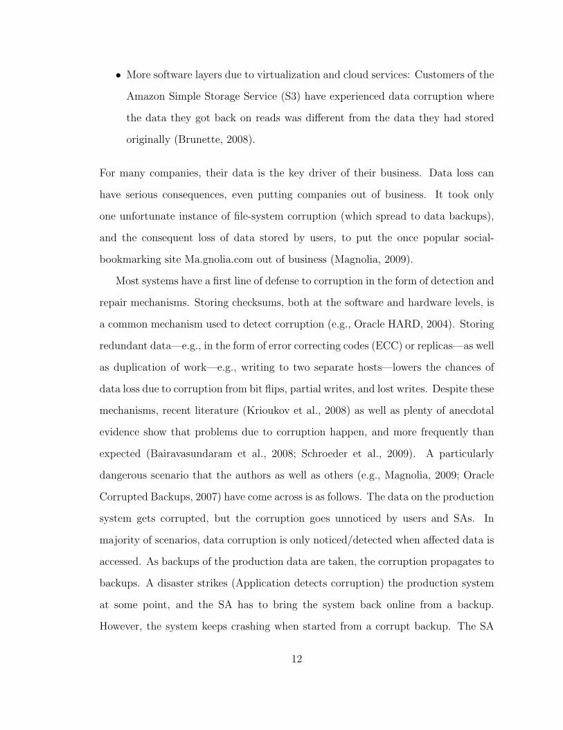
• More software layers due to virtualization and cloud services: Customers of the
Amazon Simple Storage Service (S3) have experienced data corruption where
the data they got back on reads was different from the data they had stored
originally (Brunette, 2008).
For many companies, their data is the key driver of their business. Data loss can
have serious consequences, even putting companies out of business. It took only
one unfortunate instance of file-system corruption (which spread to data backups),
and the consequent loss of data stored by users, to put the once popular social-
bookmarking site Ma.gnolia.com out of business (Magnolia, 2009).
Most systems have a first line of defense to corruption in the form of detection and
repair mechanisms. Storing checksums, both at the software and hardware levels, is
a common mechanism used to detect corruption (e.g., Oracle HARD, 2004). Storing
redundant data—e.g., in the form of error correcting codes (ECC) or replicas—as well
as duplication of work—e.g., writing to two separate hosts—lowers the chances of
data loss due to corruption from bit flips, partial writes, and lost writes. Despite these
mechanisms, recent literature (Krioukov et al., 2008) as well as plenty of anecdotal
evidence show that problems due to corruption happen, and more frequently than
expected (Bairavasundaram et al., 2008; Schroeder et al., 2009). A particularly
dangerous scenario that the authors as well as others (e.g., Magnolia, 2009; Oracle
Corrupted Backups, 2007) have come across is as follows. The data on the production
system gets corrupted, but the corruption goes unnoticed by users and SAs. In
majority of scenarios, data corruption is only noticed/detected when affected data is
accessed. As backups of the production data are taken, the corruption propagates to
backups. A disaster strikes (Application detects corruption) the production system
at some point, and the SA has to bring the system back online from a backup.
However, the system keeps crashing when started from a corrupt backup. The SA
12
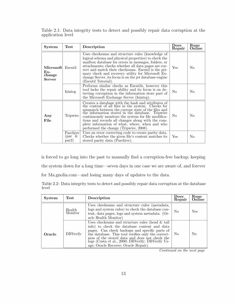
Table 2.1: Data integrity tests to detect and possibly repair data corruption at theapplication level
System Test Description DoesRepair
RunsOnline
MicrosoftEx-changeServer
Eseutil
Uses checksums and structure rules (knowledge oflogical schema and physical properties) to check themailbox database for errors in messages, folders, orattachments; checks whether all data pages are cor-rect and match their checksums. Eseutil is the pri-mary check and recovery utility for Microsoft Ex-change Server, its focus is on the jet database engine(Eseutil Tutorial).
Yes No
IsintegPerforms similar checks as Eseutils, however thistool lacks the repair ability and its focus is on de-tecting corruption in the information store part ofthe Microsoft Exchange Server (Isinteg).
No No
AnyFile
Tripwire
Creates a database with the hash and attributes ofthe content of all files in the system. Checks formismatch between the current state of the files andthe information stored in the database. Tripwirecontinuously monitors the system for file modifica-tions and records all changes along with the com-plete information of what, where, when and whoperformed the change (Tripwire, 2008).
No No
Parchive(par &par2)
Uses an error correcting code to create parity data.Checks whether the given file’s content matches itsstored parity data (Parchive).
Yes No
is forced to go long into the past to manually find a corruption-free backup; keeping
the system down for a long time—seven days in one case we are aware of, and forever
for Ma.gnolia.com—and losing many days of updates to the data.
Table 2.2: Data integrity tests to detect and possibly repair data corruption at the databaselevel
System Test Description DoesRepair
RunsOnline
Oracle
HealthMonitor
Uses checksums and structure rules (metadata,logs and system rules) to check the database con-tent, data pages, logs and system metadata. (Or-acle Health Monitor)
No Yes
DBVerify
Uses checksums and structure rules (head & tailinfo) to check the database content and datapages. Can check backups and specific parts ofthe database. This tool verifies only the correct-ness of the stored data and does not check thelogs (Costa et al., 2000; DBVerify; DBVerify Us-age; Oracle Recover; Oracle Repair).
No No
Continued on the next page
13
Table 2.2 – Continued from the previous page
System Test Description DoesRepair
RunsOnline
DBMS Re-pair
Uses checksums and structure rules (metadataand system rules) to check and repair all tablestructures, marks data pages as corrupted if thereis a checksum mismatch. This tool will repair cor-rupted table structures but will not recover data(DBMS Repair; Oracle Recover; Oracle Repair).
Yes No
RMAN
Performs backups and uses checksums and struc-ture rules (metadata, logs and system rules) tofind corrupted data pages and restored them froma backup (Oracle Recover; Vargas, 2008).
Yes No
DB2
db2inspect,Inspectcommand
Uses checksums and structure rules (page head-ers, properties of records) to check the database,data pages, records and the database memorystructures (DB2 Inspect Command; db2inspectTool; Inspect vs db2dart).
No Yes
db2dart
Uses checksums and structure rules (page head-ers, properties of records) to check and repair thedatabase, data pages, and records (db2dart Tool;Inspect vs db2dart).
Yes No
Check Data,Check In-dex
Use checksums and structure rules (table and in-dex metadata) to check the table data pages, in-dex data pages and index entries point to the cor-rect records (DB2 Check Utilities).
No Yes
db2ckbkp
Uses checksums and structure rules (metadataand page headers) to check the data page con-sistency in a backup. Determines if a backup isvalid for restore operation (db2ckbkp Tool).
No No
MicrosoftSQLServer
Checkdb,Check-table
Use structure rules (page headers, properties ofindexes) to check and repair storage of the datapages and index entries point to the correctrecords (SQL Server checkDB).
Yes No
RestoreUses backups to restore and recover the fulldatabase content, tables, data pages and logs(SQL Server Restore Command).
Yes No
MySQL
myisamchk
Uses checksums and structure rules (flags, tablemetadata) to check and repair data pages, recordsand indexes to point to correct records. Thissuite contains 5 distinct tests that do increasinglyrigorous and time-consuming checks (myisamchkCommand; Subramanian et al., 2010).
Yes No
mysqlchk
Uses checksums and structure rules (flags, tablemetadata) to check and repair data pages, recordsand indexes to point to correct records. Worksagainst all storage engines, but its functionalityis limited by the storage engine API (mysqlcheckCommand; Subramanian et al., 2010).
Yes Yes
End of Table 2.2
14
Table 2.3: Data integrity tests to detect and possibly repair data corruption at the file-system level
System Test Description DoesRepair
RunsOnline
XFS
xfs check
Uses the file-system’s journal (log of operationsdone) and verifies the integrity of the inode hi-erarchy and that the content of the inodes is insync with the stored file-system data. Checks su-perblock, free-space maps, inode maps and datablocks (Fixing XFS).
No No
xfs repair
Uses the file-system’s journal (log of operationsdone) to repair the integrity of the inode hierarchyand the connections between the the content of theinodes and the stored file-system data. Repairs su-perblock, free-space, and inode maps (Fixing XFS).
Yes No
Ext3 &Ext4
fsck
Uses the journal (in ext4) and file structures (inext3) to check the superblock, file pathnames, datablock connectivity, and the file and inode referencecounts (Admin’s Choice, 2009).
Yes No
StellarPhoenixRecovery
Uses the journal (in ext4) and file structures (inext3) to recover lost files and folders, and the su-perblock content and placement (Stellar PhoenixLinux Data Recovery).
Yes No
FAT* &NTFS
ScanDiskUses file structures to check the disk headers,FAT media, file content, file attributes, lost diskspace, incorrect free space, internal clusters, andfile crosslinks (Quirke, 2002).
Yes No
ChkDskUses file structures and the physical structure of adisk to check the file content, file attributes, freedisk space, and file crosslinks (Laurie, 2011).
Yes No
ZFS zpoolscrub
Uses built-in block checksums and block replica-tion mechanisms in the ZFS file-system to check filecontent for errors. ZFS built-in redundancy (rang-ing from mirroring to RAID-5) with the transac-tion Copy-on-Write (COW) mechanism are used torepair block corruptions (Hablador, 2009; Cromar,2011; Sun Microsystems ZFS, 2006; Zhang et al.,2010).
Yes Yes
End of Table 2.3
Table 2.4: Data integrity tests to detect and possibly repair data corruption at thehardware level
System Test Description DoesRepair
RunsOnline
HardDiskDrive
Scrubbing
Uses checksums stored at the level of disk mediablocks to verify that each block’s content matchesits checksum. Each hardware vendor has a spe-cific implementation of the scrubbing algorithm(Schwarz et al., 2004).
No No
RAID ScrubbingUses stored parity information or replicas at theRAID level (instead of per disk) to verify the con-tent of each data block (Krioukov et al., 2008).
Yes Yes
15
Thus, systems have developed a second line of defense in the form of data-integrity
tests (hereafter, tests). A test: (a) performs checks in order to detect specific types
of data corruption, and/or (b) repairs specific types of data corruption. Just like
software bugs, prevention is better than cure in the case of data corruption. However,
prevention is not always possible. Tables 2.1, 2.2, 2.3 and 2.4 list popular tests
for detecting and repairing corruption that occur in different systems as well as in
different system layers such as storage, file-system, and database. Tests have the
following characteristics:
• Tests perform more sophisticated detection and repair of corruption than is
possible automatically during regular system operation through mechanisms
like checksums and RAID (Subramanian et al., 2010).
• Barring few exceptions, tests have been developed to be run offline when the
system is not serving a workload. If a workload changes the data concurrently
with a test execution, the test may detect (and worse, fix) spurious corruptions.
The workload could also return incorrect results because of modifications made
by the test. As one example, it is recommended that the file-system be un-
mounted while running the fsck test.
• Most of the tests are very resource-intensive.
Because of the above characteristics of tests, database and storage SAs often struggle
with questions on when and where to run tests. If the SA is not proactive in running
tests, then, when corruption strikes eventually, high system downtime and data loss
(and possibly, loss of the SA’s job) will result.
SAs usually have specific objectives in mind for proactive detection and repair
of data corruption. Table 2.5 gives examples of such objectives. To our knowledge,
no system today helps SAs specify objectives like these easily, and automates the
16
Table 2.5: Examples of objectives that a SA may have regarding timely detectionand repair of data corruption
Description of Example Objectives in English1 If the myisamchk test detects corruption in the lineitem table in my MySQL OLTP
DBMS, then I want to have immediate access to an older corruption-free version ofthe table that is less than 1 hour old.
2 (A security vulnerability patch was applied in the ext4 file-system that my pro-duction DBMS is using. I am afraid that the patch may inadvertently cause datacorruption.) Run the fsck file-system test at least once every hour. Notify meimmediately of any corruption detected.
3 My production DBMS runs on an Amazon EC2 m1.large host. I have the sameobjectives as in 1, but I am willing to spend up to 12 dollars per day for additionalresources on the Amazon cloud to meet these objectives. How recent of a corruption-free version of the data can I have immediate access to if a corruption were to bedetected?
4 My objectives are a combination of 1 and 2, but I want the time intervals to be 30minutes instead of 60. I am cost conscious. What minimum number of m1.smallEC2 hosts should I rent to run tests?
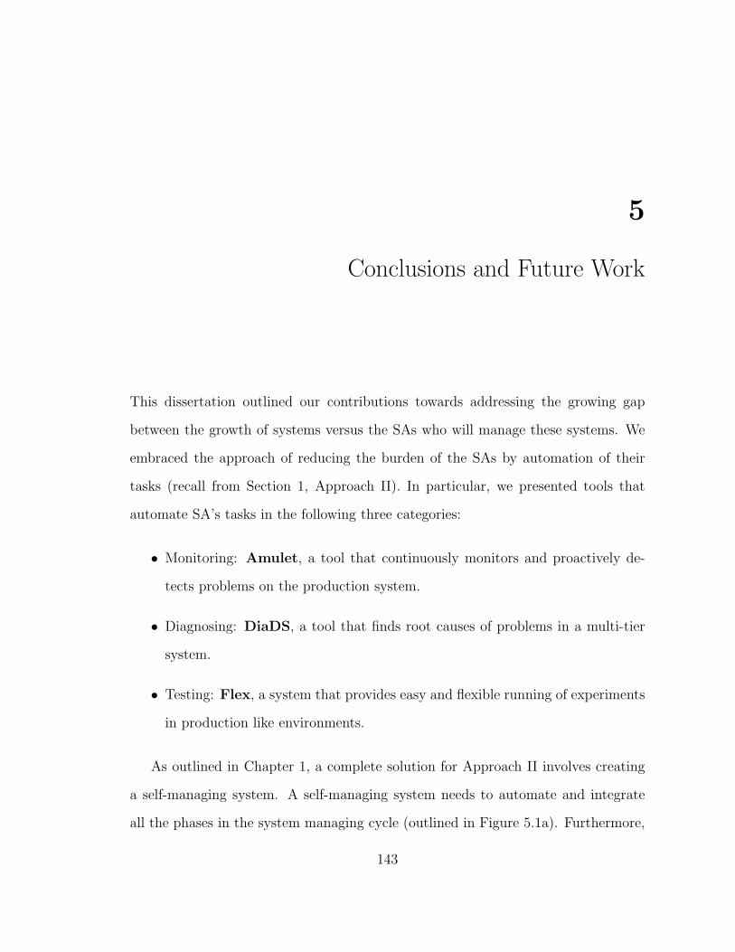
nontrivial task of running tests to meet these objectives. The result is usually a
convoluted mix of ad hoc scripts and testing practices with nobody having a clear
idea of the downtime and data loss a potential corruption can cause. In an informal
survey we conducted among SAs of clients of a large company, a pressing need to
improve the current state of testing was expressed.
2.1.1 Amulet: Challenges and Overview
A typical database software stack that production systems use is shown in Figure 2.1.
Different levels of the software stack maintain different sources of data. All these
data sources have to be kept corruption-free to guarantee correct behavior, good
performance, and availability of applications running on the software stack.
The database level has data in tables as well as plenty of metadata such as indexes,
materialized views, and information in the database catalog. Databases store their
data and metadata as files and directories in a file-system or directly as blocks on
volumes. The file-system level has files containing data stored by the database level,
as well as metadata such as the directory structure, inodes (indexes storing file-to-
Figure 2.2: Actual execution timeline, in minutes, of a testing plan in Amulet forExample 1 from Table 2.5. Each box denotes a run of the myisamchk (TM) test onthe respective snapshot Si. The horizontal width of each box corresponds to the testexecution time.
block mappings) and journals (log of operations done). A file-system, in turn, stores
its own data and metadata on a volume. A volume provides an interface to read and
write blocks of data. Beneath this interface, the volume may be a physical block
device (e.g., a hard disk or solid state drive) or a logical entity (e.g., representing
storage on a networked server or a combination of partitions from multiple hard
disks).
Proactive Testing for Data Corruption: Tests are run to verify the correctness
of data. Tables 2.1, 2.2, 2.3 and 2.4 list commonly-used tests at each level of the
database software stack. For example, MySQL’s myisamchk suite contains five differ-
ent tests invoked through distinct invocation options: fast, check-only-changed, check
(default), medium-check, and extended-check. These tests apply checks of increas-
18
ing sophistication and thoroughness to verify the correctness of tables and indexes in
the database. The checks include verifying page-level and record-level checksums as
well as verifying that each index entry points to a valid record in the corresponding
table, and vice versa. The fsck and xfs check tests verify the correctness of metadata
and data in the ext3 and XFS file-systems respectively. For example, they ensure
consistency between the file-system journal and the data blocks, and verify that all
the data block pointers in the inodes are correct.
The first challenge that Amulet faces is how to run a test automatically. Most of
the tests in Tables 2.1, 2.2, 2.3 and 2.4 cannot be run concurrently with the regular
workload on the production system because of performance and correctness problems.
The tests can consume significant CPU or I/O resources. The tests may also have to
lock large amounts of data, making response times for the production workload slow
and unpredictable. Amulet addresses these problems using the following three-step
approach to run tests automatically:
1. Create snapshot: A snapshot is a persistent copy of a point-in-time version
of the data needed for a test. Snapshots can be taken at the database, file-
system, or volume levels. In this work, we focus on volume-level snapshots
because they capture the data needed for any test in the software stack. While
the time to create the first snapshot will depend on the volume size, later
snapshots only need to copy the changes since the last snapshot (similar to
incremental backups).1
2. Run tests: A snapshot is loaded on to one or more testing hosts where tests are
run. As shown in Figure 2.1, testing hosts are different from the production
host to avoid performance problems.
1 Production deployments that need near-real-time disaster recovery take snapshots regularly andstore them on cloud storage (Wood et al., 2010).
19
3. Apply changes: If tests detect and repair corruption in a snapshot, then the
administrator can choose to apply these changes or load the repaired snapshot
on the production system.
Amulet’s Declarative Language: Making it easy and intuitive for administrators
to declare objectives like those in Table 2.5 poses a nontrivial language design prob-
lem. A dissection of the examples in Table 2.5 reveals the important features that
are needed:
• Specification of one or more tests t, and associating t with the data and type
of resources on which it should be run.
• Specification of tested recovery points to be maintained over a recent window
of time. These points enable quick system recovery in case serious corruption
is detected.
• Ability to declare different objectives such as the minimum number of test runs
per time window or a cost budget for provisioning pay-as-you-go resources to
run tests.
• Ability to combine multiple objectives as well as to specify an optimization
objective.
Angel, Amulet’s declarative language, is designed to support such features. The
semantics and simplified syntax of Angel are described in Section 2.4 and Table 2.7.
Amulet’s Optimization Phase: Amulet can run a comprehensive suite of tests,
including new user-defined ones, to detect and possibly repair data corruption any-
where in the software stack. To use Amulet, as shown in Figure 2.1, a user or
application submits a declarative Angel program that references one or more vol-
umes on the production system. For each volume V , the program specifies: (a) the
20
tests to be run on data contained in V , and (b) the objectives to be met. For volume
V , Amulet’s Optimizer will generate an efficient execution strategy—called a testing
plan—using an optimization algorithm that maximizes or minimizes one objective
subject to satisfying all other objectives. Amulet’s Orchestrator will execute the test-
ing plan automatically and continuously by provisioning testing hosts and scheduling
tests on a resource provider.
Figure 2.2 shows an actual execution timeline of a testing plan P for an Angel
program corresponding to Example 1 from Table 2.5. Plan P uses one testing host
that runs the myisamchk test on snapshots taken from the production host. One
snapshot is tested every 30 minutes, and each test takes around 20 minutes to com-
plete. As we will see in Section 2.7, this plan minimizes execution cost while meeting
the objective of continuously maintaining a tested recovery point for a past 1-hour
window. This testing plan, while simple, illustrates a number of challenges facing
Amulet.
Characterizing the testing plan space: A testing plan has multiple aspects. First,
there is a provisioning aspect that determines how many testing hosts are used to
meet the specified objectives. Second, there is a scheduling aspect that determines
the rate at which snapshots are tested and how test runs are scheduled on the provi-
sioned hosts. Third, there is a sustainability aspect that determines whether the plan
will continuously meet the specified objectives as time progresses. Section 2.5 gives
a formal characterization of a testing plan in Amulet, thereby defining the space of
testing plans.
Developing a cost model for tests: To find whether a plan enumerated from the testing
plan space will meet the objectives specified in an Angel program, the Optimizer
needs models to estimate the execution times of tests scheduled by the plan. A
novel component of Amulet is a library of models to estimate test execution times.
21
The library currently covers tests for the MySQL database and the ext3 and XFS
file-systems; discussed further in Section 2.3.
Finding a good testing plan: For each volume referenced in an Angel program, the
Optimizer has to find a good plan from a huge plan space. We propose a novel
algorithm for this optimization problem that considers all three aspects of testing
plans: provisioning testing hosts, scheduling tests on snapshots and hosts, and ensur-
ing plan sustainability over time. While our algorithm is not guaranteed to find the
optimal plan, we show empirically—based on comparisons with an exhaustive search
algorithm—that our algorithm is very efficient and finds the optimal plan most of
the time.
Amulet’s Orchestration Phase: After submitting an Angel program, the admin-
istrator can view the testing plans generated, and when satisfied, submit the plans to
Amulet’s Orchestrator for execution. The Orchestrator executes testing plans contin-
uously by working in conjunction with a Snapshot Manager and a resource provider,
both of which are external to Amulet. The Snapshot Manager notifies the Orches-
trator when a new snapshot of a volume on the production system is available for
testing. The Orchestrator allocates testing hosts from the resource provider which,
currently, can be any infrastructure-as-a-service cloud provider. A major challenge
faced by the Orchestrator is in dealing with unpredictable events arising during plan
execution:
• Repairs: It is impossible to predict when a corruption will be detected and a
repair action needs to be taken.
• Straggler hosts: A host used to run tests on the cloud may become slow
temporarily, causing the test execution schedule to lag behind the optimizer-
planned schedule.
22
• Wrong estimates: Lags in the testing schedule can also be caused by inaccurate
estimates of test execution times from the models.
Rather than complicating the Optimizer or making unrealistic assumptions, Amulet’s
solution is to reserve a cost budget in each testing plan that the Orchestrator can use
to provision additional hosts on demand to deal with unpredictable events; discussed
in Section 2.6. The novel effect is that a testing plan has a statically-planned com-
ponent generated by the Optimizer as well as an adaptive component managed by
the Orchestrator. Section 2.7 will present comprehensive experimental results from
a prototype of Amulet running on the Amazon cloud.
2.2 Related Work
A number of recent empirical studies show that corruption of critical data is a reality
and occurs much more commonly than assumed previously. It is perhaps surprising
that the database research community has paid little attention to this problem.
2.2.1 The Dangers of Data Corruption
Bairavasundaram, Goodson, Schroeder, Arpaci-Dusseau, and Arpaci-Dusseau ana-
lyzed corruption instances recorded in more than 10,000 production and development
storage systems. Their main focus was on studying silent data corruption which is
corruption undetected by the disk drive or by any other hardware component. Among
corruption instances logged over a 41-month period among a total of 1.53 million disk
drives of various types, the authors found more than 400,000 instances of checksum
mismatches. The study also showed that cheaper nearline SATA disks (and their
adapters) develop checksum mismatches an order of magnitude more often than the
more expensive and carefully-engineered SCSI disks. However, corruption can also
occur in the latter which are enterprise-class drives.
23
Schroeder, Pinheiro, and Weber analyzed memory errors collected over a period
of 2.5 years in the majority of servers used by Google. The authors found that
the rate of data corruption in DRAM is orders of magnitude higher than previously
reported, with more than 8% of dual in-line memory modules (DIMMs) affected by
errors per year. Memory errors can be classified into soft errors, that corrupt bits
randomly but do not leave physical damage; and hard errors, that corrupt bits in a
repeatable manner because of a physical defect. Memory errors found in the study
were dominated by hard errors, rather than soft errors as assumed previously.
Injecting faults into the database software stack provide insights into system
behavior and data loss under different types of corruption. A recent study used fault
injections into a popular open-source DBMS (MySQL) to show that certain types
of data corruption can harm the system, e.g., causing system crashes, data loss,
and incorrect results (Subramanian et al., 2010). The authors also point out that
concurrency control and recovery features of database systems are not designed to
detect or repair corrupted data or metadata resulting from hardware, software, or
human errors. A similar study has been done for the ZFS file-system that, compared
to popular Linux file-systems like ext3 and XFS, has novel features like end-to-end
checksums for corruption detection (Zhang et al., 2010). The authors show that while
ZFS is very resilient to disk-level corruption, memory-level corruption can lead to
crashes and incorrect results.
2.2.2 Dealing with Data Corruption
The techniques categorized as the first line of defense in Section 2.1 check for data
correctness during reads and writes in the production workload; usually based on
additional stored information like parity bits and checksums. These techniques are
not sufficient to prevent or detect corruption caused by complex issues such as lost
and misdirected writes due to bugs in the software stack (Bairavasundaram et al.,
24
2008). For example, Krioukov, Bairavasundaram, Goodson, Srinivasan, Thelen,
Arpaci-Dusseau, and Arpaci-Dusseau show the inability of techniques like parity-
based RAID to avoid data corruption. The authors also show how common tech-
niques used in RAID can spread data corruption across multiple disks and cause
data loss. The first line of defense adds performance overheads during workload exe-
cution. Graefe and Stonecipher present a technique for an online B-tree verification
with minimum overhead. However, enterprise systems have historically preferred
performance over the (wrongly assumed) rare chance of data corruption. Amulet
addresses these problems by enabling complex and resource-intensive tests like those
in Tables 2.1, 2.2, 2.3 and 2.4 to be run in a timely fashion. To our knowledge,
Amulet is the first system of its kind that works across different point-in-time copies
of data to detect and repair data corruption efficiently in the end-to-end software
stack.
System designers take different approaches to tackling data corruption. Some
systems are designed resilient, i.e., end-to-end checksums, parity/checksum verifica-
tions at every level in the system stack in the datapath, where as others rely on
offline detection tools or utilities. Modern file-systems like ZFS fall under the former
category. Most enterprise systems fall under the latter category, sacrificing integrity
in favor of performance. Due to proprietary nature of these applications, detection
and correction utilities are also tightly controlled by the vendors. Section 2.3 and
Tables 2.1, 2.2, 2.3 and 2.4 provided a fairly comprehensive listing of tests used in
systems today.
Modeling the performance of tests or improving their efficiency has received little
attention. For example, most tests still use single-threaded execution and cannot
exploit multicore CPUs. Currently, every test t is an opaque execution script to
Amulet apart from the model used to estimate t’s execution time. With more visi-
bility into tests, Amulet can do a better job of optimizing t’s execution. A promising
25
development in this regard is the writing of tests in declarative languages like SQL
as done by Gunawi et al. (2008).
Amulet’s goal of early detection and repair of data corruption forms a crucial
part of disaster recovery planning. Wood, Cecchet, Ramakrishnan, Shenoy, van der
Merwe, and Venkataramani argue that cloud computing platforms are well suited for
offering disaster recovery as a service due to (a) the cloud’s pay-as-you-go pricing
model that can lower costs, and (b) the cloud’s use of elastic virtual platforms.
Amulet is a proof-of-concept system for this argument applied to the problem of
data corruption.
The concept of declarative system management is gaining currency. Chef, Pup-
pet, and Microsoft SQL Server’s policy-driven manager are now popular tools that
take declarative specifications as input, and then configure and maintain systems au-
tomatically (Guo et al., 2009). However, unlike Amulet, these tools do not support
objectives that are specified declaratively and optimized automatically.
2.3 Modeling of Tests
For each test t, Amulet’s Optimizer needs a model to estimate t’s run-time behavior—
e.g., execution time, usage of CPU, memory, and I/O resources—when t is run on
given data and system resources. We divide the input parameters for a test model into
three categories: (i) data-dependent attributes, (ii) resource-dependent attributes,
and (iii) attributes to capture transient effects. In this section, we discuss attributes
in the test model and their impact for the myisamchk, fsck, and xfs check tests from
Tables 2.2 and 2.3. Our focus is on models for estimating test execution time. Note
that we generate separate models for the same test when invoked with significantly
different options. For example, fsck has separate models based on whether it is
invoked to check file-system metadata compared to data. The fsck metadata test
26
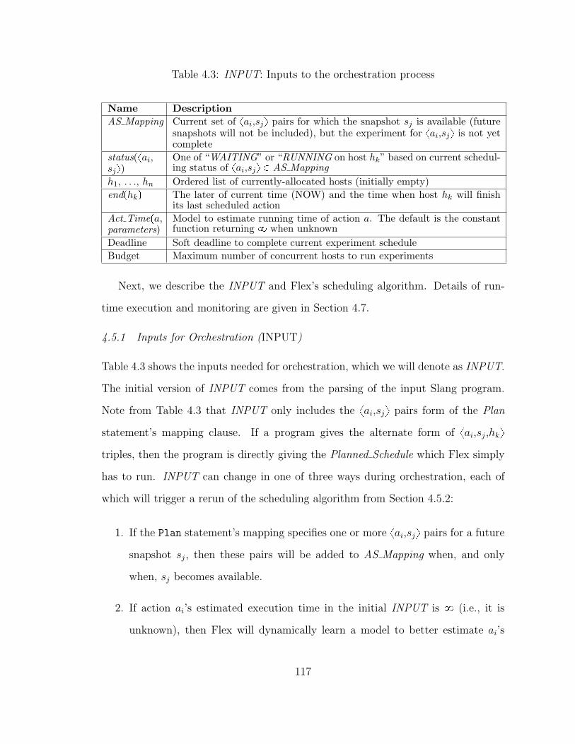
0 20 40 60 80 100 120 140 160 180 2000
5
10
15
20
25
30
35
40
45
File-system Size (in GB)
Co
mp
leti
on
Tim
e (
min
)
(a) Varying the file-system size for fsck test onext3
0 1 2 3 4 5 6 7 8 9 10 110
20
40
60
80
100
120
140
160
180File size =1 KB File size = 64 KB
Used Inodes (in millions)
Co
mp
leti
on
Tim
e (
min
)
(b) Varying the number of used inodes forxfs check on XFS
plans) over potential optimality since the former is more important in proactive
testing.
Warm Vs. cold caches: Data caching for the memory/disk interface within a host
does not benefit tests such as fsck and xfs check that access data directly at the block
level. However, as mentioned before, such caching benefits higher-level tests such
as myisamchk. Data caching at the host/network interface while using networked
storage benefits most tests. We have observed up to 2x differences in test execution
times for warm Vs. cold caches in this context. The test models have been enhanced
to account for these effects.
2 We did manage to improve the execution time of the fsck data test by 40% using software-RAID-like techniques on the Amazon cloud.
30
Concurrent execution of tests on the same host: Concurrent execution makes test
execution times difficult to estimate. Figure 2.4c illustrates this complexity. Test sets
1 and 2 are runs of two myisamchk tests on two different tables. The tests in each
set lead to different outcomes when run in concurrent versus sequential fashion. The
tests in set 2 cause memory thrashing when run concurrently. Since the number of
distinct tests is not large,3 we can train models to estimate execution times for tests
run concurrently in pairs. As such, if Amulet’s Optimizer does not have a model to
estimate the running time of concurrent tests, it will simply choose not to consider
testing plans with concurrent tests. The goal of the Optimizer is to find a robust
testing plan, where a robust plan is one whose performance is almost never much
worse than promised.
Time-of-day effects: External workload on the IaaS provider may influence the test
completion time. However, for our test bed with Amazon we did not observe any
significant variation in the test run-times as a function of time-of-day.
In summary, there are only a few popular tests, so test models can be built
once and reused. As Amulet controls the resource on which tests are run, the tool
can ensure that tests are run in similar settings to the one used for the modeling.
Furthermore, the discretization and isolation provided by the cloud environment
significantly helps limit the attribute permutations in the models.
2.4 The Angel Declarative Language
This section and Table 2.7 summarizes the main statements in the Angel 4 declarative
programming language. An Angel program specifies tests as well as the objectives
3 From our experience, most SAs prefer to use standard tests that come with each system, ratherthan writing new tests.
4 Angel script was a form of writing used by the philosopher-king Solomon in amulets he designedfor various life’s problems (King Solomon’s Amulets)
31
Table 2.6: Notation used in this chapter
Name DescriptionO1-On SSO, RPO, SIO, TCO, or CO objectives specified per volume in an
Angel program (Table 2.7 gives a summary)Oopt Optimization objective for a volume in an Angel programt, s, h, τ , x,and d
Used to denote respectively tests, volume snapshots, hosts, time inter-vals, numeric constants, and currency values
τrpo The time interval in an RPO (see Table 2.7)dco The maximum cost budget in a CO (see Table 2.7)P Testing plan for a volume in an Angel programPW Plan P ’s window. The plan repeats every PW time unitsPI Time interval between successive snapshots in plan P
PM Test-to-snapshot mapping in plan P
PS Schedule of test execution in plan P
PR P ’s cost budget reserved to handle unpredictable eventsExecTimeptq Execution time of test tTimepsiq Time when ith snapshot si, 1 ¤ i ¤ PW
PI, is available in plan P relative
to the start of the plan window PWstartphq Time when host h is first used in the plan windowendphq Time when host h will finish its last scheduled test for the plan window
(endphq can be ¡ PW )costpPSq,costphq
Cost incurred for the plan schedule PS or a host h for one plan window
to be met while running these tests. Figure 2.5, which we will use for illustration in
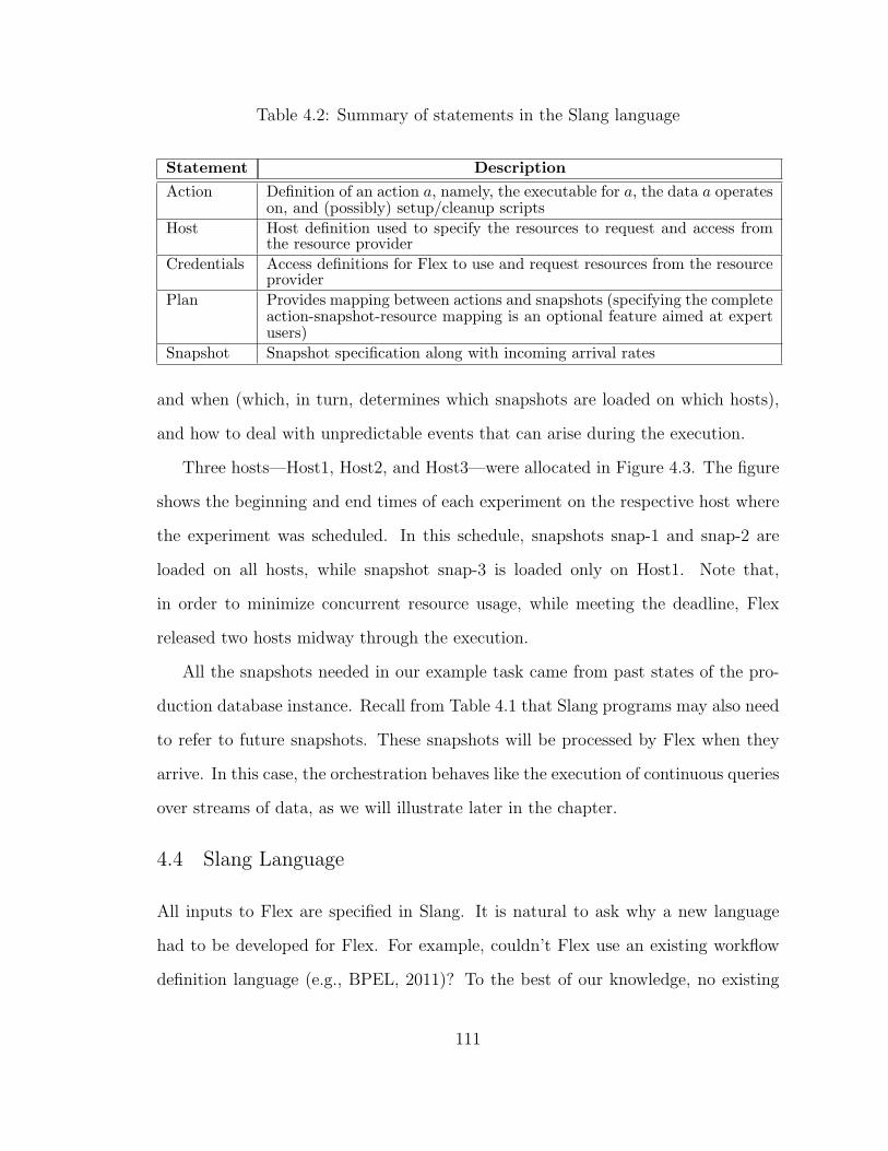
this section, shows an Angel program for Example 1 in Table 2.5.
Tests: Angel’s Test statement defines a test t by specifying the command to run t
as well as references to t’s input data (specified by a Data statement) and the type of
host on which to run t (specified by a Host statement). The Test lineCheck state-
ment in Figure 2.5 defines the myisamchk medium test for MySQL from Table 2.2.
Angel’s Repair statement enables a repair action to be associated with a test t for
invocation if t detects a corruption (as indicated by a specific return code from t).
Data: Angel’s Data and related statements define the input data for a test, including
the volume that the data belongs to, the data type (from a set of supported types),
and the data properties. The properties, which are specific to the type of data, form
inputs to the models that the Optimizer uses to estimate test execution times. The
32
Table 2.7: Summary of important Angel statements. Op P t¤,¥u. t, τ , x, and d areconstants of respective types test, time interval, numeric, and currency
Name Simplified Specification SyntaxTest Test(Data: data, Host: host, exec scripts, . . .)Input data for test Data(Volume: V , type, properties, . . .)Host to run test Host(type, setup scripts, . . .)Volume Volume(Host: production host where V is located,
path on host, volume id, properties, . . .)Repair action Repair(Test: t, t’s return code, exec scripts, . . .)SSO: Safe Snapshot Objective List of tests tt1, t2, . . . , tku, for volume VRPO: Recovery Point Objec-tive
Recovery point ¤ τ , for volume V
SIO: Snapshot Interval Objec-tive
Snapshot interval Op τ , for volume V
TCO: Test Count Objective Test countptq Op x, in time interval τ , for volume VCO: Cost Objective Cost ¤ d, in time interval τ , with reservation x%, for
volume VOopt: Optimization Objective Maximize (when Op is ¥ in an SIO or TCO), Minimize
(when Op is ¤ in an RPO, SIO, or CO)Notification SQL triggers on event tables in log database
Optimizer does semantic checks to ensure that the Angel program specifies values
for all input parameters required by the model for each test in the program. While
helper tools are available to extract these values from the corresponding input data,
the SA can also specify values based on their domain knowledge.
Hosts: The primary use of Angel’s Host statement is to define a host type (from a
set of supported types) for a test t so that the Orchestrator guarantees that t will
always be run on hosts of that type. Figure 2.5 shows 2 host definitions (prodHost
and testHost). The current implementation of the Orchestrator supports all the EC2
host types on the Amazon cloud.
2.4.1 Objectives
An Angel program can specify one of five types of objectives. These objectives can
be used independently or combined together to specify a variety of requirements for
running tests. Each objective O references a unique volume. The Optimizer will
Figure 2.5: Angel program for Example 1 in Table 2.5
partition the objectives in an Angel program based on the volumes referenced, and
generate one testing plan per volume.
Safe Snapshot Objective (SSO): An SSO for a volume V specifies a list of tests
t1,. . .,tk that Amulet must run on every snapshot s given for V by the Snapshot
Manager. Note that a volume-level snapshot will contain the input data needed
for any test. (The Optimizer checks to ensure semantic consistency across all the
statements in a program.) If none of the tests t1,. . .,tk find corruption on s, then
Amulet will label s as corruption-free. If a repair action is associated with a test t,
then Amulet will run the repair on snapshot s if t were to detect a corruption in s.
Recovery Point Objective (RPO): When one or more tests detect corruption in
a snapshot of a volume V , it is useful to have another snapshot of V in the recent
past where the corruption did not exist. This objective usually arises from recovery
needs. If a corruption causes an application to crash or misbehave, then the SA may
have to find a recent recovery point quickly (Wood et al., 2010). A recovery point
34
����������
���
���� ��� ���� ��������� �����
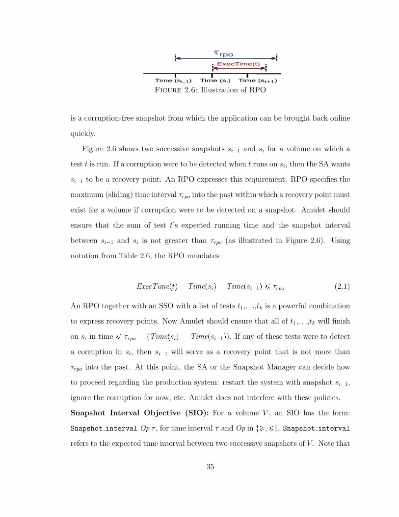
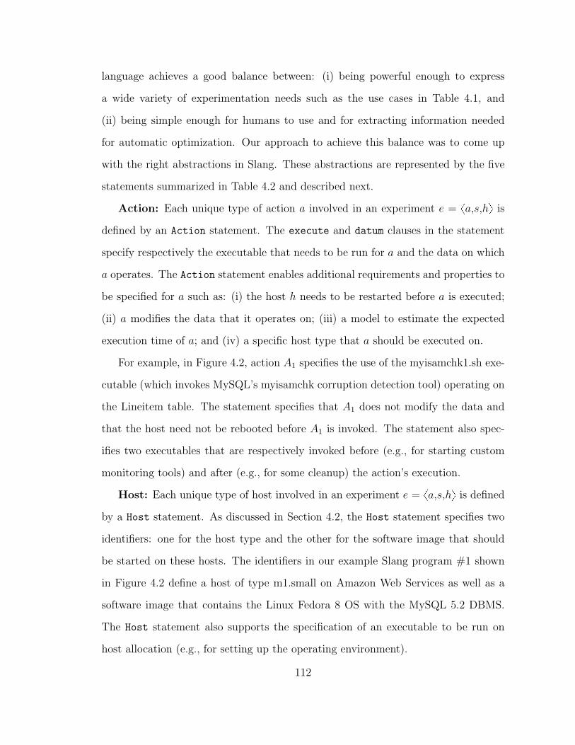
Figure 2.6: Illustration of RPO
is a corruption-free snapshot from which the application can be brought back online
quickly.
Figure 2.6 shows two successive snapshots si�1 and si for a volume on which a
test t is run. If a corruption were to be detected when t runs on si, then the SA wants
si�1 to be a recovery point. An RPO expresses this requirement. RPO specifies the
maximum (sliding) time interval τrpo into the past within which a recovery point must
exist for a volume if corruption were to be detected on a snapshot. Amulet should
ensure that the sum of test t’s expected running time and the snapshot interval
between si�1 and si is not greater than τrpo (as illustrated in Figure 2.6). Using
notation from Table 2.6, the RPO mandates:
ExecTimeptq � Timepsiq � Timepsi�1q ¤ τrpo (2.1)
An RPO together with an SSO with a list of tests t1,. . .,tk is a powerful combination
to express recovery points. Now Amulet should ensure that all of t1,. . .,tk will finish
on si in time ¤ τrpo � (Timepsiq � Timepsi�1q). If any of these tests were to detect
a corruption in si, then si�1 will serve as a recovery point that is not more than
τrpo into the past. At this point, the SA or the Snapshot Manager can decide how
to proceed regarding the production system: restart the system with snapshot si�1,
ignore the corruption for now, etc. Amulet does not interfere with these policies.
Snapshot Interval Objective (SIO): For a volume V , an SIO has the form:
Snapshot interval Op τ , for time interval τ and Op in t¥,¤u. Snapshot interval
refers to the expected time interval between two successive snapshots of V . Note that
35
Amulet does not control the Snapshot Manager which collects snapshots from the
production system. SIOs express the feasible snapshot intervals that Amulet should
consider during plan selection.
Test Count Objective (TCO): For a volume V , a TCO has the form: Test countptqOp x, in a time interval τ for a test t. Here, Test count specifies the number of
unique snapshots of V in the interval τ on which Amulet should run test t. The
typical use of TCOs are to express requirements of the form: “Run t at least four
times every day.” A plan chosen by the Optimizer for this TCO will do the intuitive
thing of spacing out the four test runs uniformly in the specified time interval of 1
day.
Cost Objective (CO): A CO for a volume V has the form: Cost ¤ d, in a time
interval τ , with (optional) reservation x. Here, d is a cost measure for the resource
provider from which the Orchestrator will allocate resources to run tests. Costs may
be specified in real or virtual currency units depending on the provider. The CO
applies to the entire testing plan that the Optimizer generates for V . For example,
a CO for the Amazon cloud could be (see Table 2.5): “The testing plan can use up
to 12 U.S. dollars per day.” A CO can be specified only if the pricing model that the
resource provider uses to charge for resource usage is input to Amulet. Section 2.7
describes the pricing model that Amulet uses for the Amazon cloud.
The CO specifies a fraction of the overall cost budget that is reserved for the
Orchestrator to respond to three types of unpredictable events that can occur during
the execution of the testing plan: repairs, straggler hosts, and inaccurate predictions
of test execution times by the models used in the Optimizer (recall Section 2.1.1).
Section 2.6 will discuss how the Orchestrator uses the reserved cost budget to pro-
vision hosts on demand to handle these unpredictable events. When Amulet is used
on the Amazon cloud, by default, the reservation is set to the cost of one host that
can run all the tests specified in the Angel program.
36
Find the Least-Cost Plan P=xPW ,PI ,PM ,PS,PRy that Satisfiesthe n Objectives O1-On (without Oopt) for a Volume V in an Angel Program
1. Use Figure 2.8 to pick the snapshot interval PI for O1-On;2. Select the plan window PW , and scale O1-On to PW (Section 2.5.3);3. Use Figure 2.9 to pick the test-to-snapshot mappingPM for O1-On,PW ,PI ;4. Use Figure 2.10 to pick the test execution schedule PS for PW ,PI ,PM ;5. PR is available from the CO in O1-On, or a default is used;
Figure 2.7: Finding the least-cost plan for given objectives O1-On
Optimization Objective (Oopt): An appropriate Maximize or Minimize optimiza-
tion objective (Oopt) can be specified along with an RPO, SIO, TCO, or CO for a
volume V in an Angel program. Maximize can be used when Op in the objective
is ¥, and Minimize can be used when Op is ¤. Specifically, applying Maximize to
an SIO or TCO of the form value ¥ const asks to make const as high as possible.
Applying Minimize to an RPO, SIO, or CO of the form value ¤ const asks to make
const as low as possible. One and only one Oopt is allowed per volume. The default
is Minimize CO if no Oopt is specified in the program.
Notifications: Users can request notifications when certain events or sequences
of events occur when a plan is executed by the Orchestrator. A comprehensive
logging framework in the Orchestrator logs a range of events of interest, including
snapshot collection, start and completion of tests, detection of corruption, application
of repairs, and lags in the testing schedule. The logs are persisted into a database
system which runs continuous queries to provide the notifications specified in the
Angel program. Our current implementation uses the PostgreSQL database system
and provides notifications using triggers.
2.5 Optimizer
In this section, we will discuss the algorithm used by Amulet’s Optimizer. Given an
Angel program, the Optimizer first partitions the objectives in the program based on
37
the volumes referenced, and then selects one testing plan per volume. The selection
of the testing plan is treated as the following optimization problem:
Testing-plan Selection Problem for Volume V : Given n objectives O1-On
(each of type SSO, RPO, SIO, TCO, or CO) and an optimization objective Oopt (of
type Maximize or Minimize on one of O1-On) for a volume V , find the testing plan
(if any) that meets all of O1-On while giving the best (maximum or minimum, as
appropriate) value for Oopt.
We will first describe the structure of a testing plan generated by Amulet’s Optimizer,
and then describe the various stages employed by the Optimizer as it attempts to
find the optimal plan from the large plan space. In Section 2.7, we will compare our
Optimizer with an exhaustive optimizer that works by systematically enumerating
plans from this large plan space (and scales poorly because of this nature).
2.5.1 Testing Plans in Amulet for a Volume V
Formally, a testing plan P contains five components:
1. Snapshot interval PI is the uniformly-spaced minimum time interval between
consecutive snapshots that the plan needs to test to meet all the objectives
specified.
2. Window PW is a time interval such that the plan repeats every PW time units.
The plan processes PW
PIsnapshots per window.
3. Test-to-snapshot mapping PM specifies, for each snapshot s in the plan window,
the set of tests that need to be run on s.
4. Test execution schedule PS specifies the number and respective types of testing
hosts to use, and when to run each test from PM on these hosts.
38
5. Reserved cost budget PR is the part of the plan’s total cost budget that is
reserved for the Orchestrator to deal with unpredictable events that can arise
during plan execution.
The core of Amulet’s Optimizer is a cost-optimal planning algorithm that can find
the minimum-cost plan (if valid plans exist) to meet a given set of objectives. We
will begin in Sections 2.5.3–2.5.5 by describing the stages in which the cost-optimal
planning algorithm works. As illustrated in Figure 2.7, each stage selects one of the
five components of the minimum-cost plan, going in the order PI , PW , PM , PS, and
PR. Section 2.6 will describe how the Orchestrator uses the reserved cost budget PR.
If the Angel program’s optimization objective is not cost minimization, then
Amulet uses a higher-level planning algorithm, described in Section 2.5.6.
We use ExecTime(t) to denote the running time of test t as estimated by the
models available to the Optimizer. If all input parameters required by the model(s)
for t have not been specified in the Angel program, then the Optimizer will catch
this error during its semantic checking phase. Since the Optimizer reads the model
for each test t from a model library, an Amulet user can override an existing model
or supply a model for a new test they have defined. A model can be as simple as a
function that always returns a constant value for ExecTime(t) (e.g., representing t’s
running time for the host type specified in the program). With this feature, the SA
can ask useful what-if questions, e.g., “how much additional cost will be needed to
meet my objectives if test execution times were to increase by x%?”.
2.5.2 Selecting the Snapshot Interval
The Optimizer’s goal in this stage is to pick the maximum value that PI can have
while meeting all the RPO, SIO, and TCO objectives specified. Maximizing PI
translates into minimizing the number of snapshots that need to be processed. Con-
39
Selecting the Plan Snapshot Interval PI in a Testing PlanInputs: Objectives O1-On (with syntax from Table 2.7)1. PminI = Snapshot interval from the Snapshot Manager;2. PmaxI = 8; τrpo = 8;3. if (O1, . . . , On contains RPO: Recovery point ¤ τ) {4. τrpo = τ ; PmaxI = τrpo
2 ; /* test ¥2 snapshots in τrpo to meet RPO */}5. for (every Objective O in O1, . . . , On) {6. if (O is SSO: List of tests tt1, . . . , tku) {7. for (Test t in t1, . . . , tk)8. PmaxI = Min[PmaxI , τrpo - ExecTime(t)]; } /* Equation 2.1 */9. if (O is TCO: Test countptq ¥ x, in time interval τ)10. PmaxI = Min[PmaxI , τrpo - ExecTime(t), τ
x ]; /* Equation 2.1 */11. if (O is SIO: Snapshot interval ¥ τ)12. PminI = Max[PminI , τ ];13. if (O is SIO: Snapshot interval ¤ τ)14. PmaxI = Min[PmaxI , τ ];15. }16. if (PmaxI PminI ) return “No feasible PI exists for O1-On”;17. else set PI � PmaxI ;
Figure 2.8: Selection of PI (notation used from Tables 2.6 and 2.7)
sequently, the cost of the plan is minimized—which is our goal—since more snapshots
mean higher test execution and host requirements.
Figure 2.8 shows the steps involved in this stage. The algorithm goes through the
objectives one by one, while maintaining an upper (PmaxI ) and lower (Pmin
I ) bound
on feasible values of PI . Finally, the largest feasible value of PI , if any, is selected.
2.5.3 Selecting the Plan Window
Recall from Section 2.4 and Table 2.7 that the objectives RPO, TCO, and CO for a
volume V in an Angel program specify time intervals. The plan window PW serves as
a mechanism for the Optimizer to consider the intervals in all objectives in a uniform
fashion. PW is picked as the least multiple of PI pPW = n � PI , n P Nq such that
PW is greater than or equal to the maximum among: (a) the time intervals in RPO,
TCO, and CO objectives, and (b) ExecTimeptq for each test t specified in an SSO
40
Selecting the Test-to-Snapshot Mapping PM in a Testing PlanInputs: Scaled objectives O1-On, Plan Window PW , Snapshot Interval PI1. for (every test t referenced in an SSO or TCO in O1, . . . , On) {2. COUNTmin
t = 0; COUNTmaxt = PW
PI; }
3. for (every Objective O in O1, . . . , On) {4. if (O is SSO: List of tests tt1, . . . , tku) {5. for (Test t in t1, . . . , tk) /* t has to run on all PW
PIsnapshots */
6. COUNTmint = Max[COUNTmin
t , PWPI
]; }7. if (O is TCO: Test countptq ¥ x, in time interval PW )8. COUNTmin
t = Max[COUNTmint , x];
9. if (O is TCO: Test countptq ¤ x, in time interval PW )10. COUNTmax
t = Min[COUNTmaxt , x];
11. }12. PM = H;13. for (every test t referenced in an SSO or TCO in O1, . . . , On) {14. if (COUNTmax
t COUNTmint ) return “No feasible PM exists”;
15. else {16. Map test t to COUNTmin
t snapshots spread uniformly across thePWPI
snapshots in the plan window. Add the mappings to PM ; }17. }
Figure 2.9: Selection of PM (notation used from Tables 2.6 and 2.7)
or TCO objective. Picking PW ¡ ExecTimeptq for all tests (i.e., Case (b) above) is
needed to ensure the sustainability of schedules as we will explain in Section 2.5.5.
Once PW has been determined, the corresponding parameters in all TCO and
CO objectives are scaled proportionately to PW . For example, a CO that specifies a
cost budget pdcoq of U.S. $10 in 1 hour, will be scaled to a cost budget of U.S. $15
for PW � 1.5 hours. Note that the time interval in an RPO (τrpo) is independent of
PW , and should not be scaled.
2.5.4 Selecting the Test-to-Snapshot Mapping
For the PW
PIsnapshots in a plan window, this stage decides which tests need to be run
on which snapshots. Figure 2.9 shows the steps involved. For each test t specified
in an SSO or TCO, the algorithm in Figure 2.9 maintains upper (COUNTmaxt ) and
41
lower (COUNTmint ) bounds on how many snapshots t should be run on. Test t is
mapped at uniformly-spaced intervals to the minimum number of snapshots that t
needs to be run on. Note that the tests in an SSO should be run on all PW
PIsnapshots
(Lines 4-6 in Figure 2.9).
2.5.5 Selecting the Schedule of Test Execution
After the test-to-snapshot mapping PM has been generated, the Optimizer selects
the schedule as well as the minimum number of hosts needed for running these tests.
This stage, whose steps are shown in Figure 2.10, is by far the most complex one
in the Optimizer. Note that the Optimizer is only identifying a good schedule. The
schedule will be executed—including actual host allocation and test runs on the
resource provider—only after the testing plan is submitted to the Orchestrator.
The self-explanatory Lines 1-13 in Figure 2.10 give an overview of the greedy
algorithm used to select the test execution schedule. The algorithm goes through
the snapshots si in one plan window in order from i=1 to i=PW
PI, as well as the tests
tij that have been mapped to si. A host hk is identified to run tij on si in one of the
three ways listed respectively in Lines 5, 7, and 9.
The first way (described in Lines 14-24) is by means of test grouping, where tij
will be run concurrently with another test or group of tests on a host that has already
been allocated to the plan. Line 16 comes from Amulet’s goal to generate a robust
plan (Babcock and Chaudhuri, 2005), i.e., a plan whose chances of performing worse
than estimated is low. If there is no model to estimate how the concurrent execution
of a set of tests will perform, then the Optimizer takes the low-risk route of avoiding
such executions.
Line 19 (similarly, Line 29) addresses the important issue of schedule sustainability
which ensures that the plan generated for one window can be run continuously for
multiple windows that come one after the other. Using notation from Table 2.6, let
42
Selecting the Schedule of Test Execution PS in a Testing PlanInputs: Plan Window PW , Snapshot Interval PI , Test mapping PM , Resource provider’s
pricing model costp...q, and Plan cost budget dco
1. PS = H;2. for (each of the PW
PIsnapshots si in PM ) {
3. for (each test tij mapped to snapshot si in PM ) {4. for (each host hk added so far to PS and whose host type matches the host type needed
to run tij) {5. [Line 14] if (tij can be scheduled by grouping tij with an already-scheduled test t1
on si and hk) {6. Update PS to add the new Groupedpt1, tijq test instead of t1 on hk.
Go to the next test; }7. [Line 25] else if (tij can be scheduled on hk after all currently-scheduled tests on hk
have completed) {8. Update PS to schedule tij on hk; Go to the next test; }9. [Line 35] else if (tij can be scheduled on a new host h1) {10. Update PS to schedule tij on h1; Go to the next test; }11. else return “Could not find a feasible schedule PS for PM”;12. }}}13. return “Minimum-cost PS is now available for the testing plan”;
14. Function invoked from Line 5: Check grouping of test tij with a (possibly grouped) test t1
scheduled on snapshot si and host hk {15. tij can be grouped with t1 if all four conditions (a)-(d) hold {
/* avoids risky plans */16. (a) A model is available to estimate grouped execution times for the types of tests t1 and tij ;17. (b) The grouping runs the tests faster than running them serially:
ExecTime(Groupedpt1, tijq) ExecTimept1q + ExecTimeptijq;18. (c) The grouping will not violate RPO:
Timepsi�1q + τrpo ¥ endphkq - ExecTimept1q + ExecTime(Groupedpt1, tijq);19. (d) The schedule with grouping is sustainable:
PW + startphkq¡ endphkq - ExecTimept1q + ExecTime(Groupedpt1, tijq);20. }21. if (tij can be grouped with t1 on hk) {22. endphkq= endphkq - ExecTimept1q+ ExecTime(Groupedpt1, tijq);23. return true; }24. else return false; }
25. Function invoked from Line 7: Check if test tij can be scheduled on host hk after allcurrently-scheduled tests complete on hk{
26. tij can be scheduled on hk if all three conditions (e)-(g) hold {27. (e) tij can be started on hk before the next snapshot si�1 arrives:
Timepsi�1q ¡ endphkq; /*smoothing the load in PW */28. (f) The new schedule will not violate RPO:
Figure 2.10: Selection of PS (notation used from Tables 2.6 and 2.7)
43
29. (g) The new schedule is sustainable:PW + startphkq ¡ Max[endphkq, Timepsi)] + ExecTimeptijq;
30. }31. if (tij can be scheduled on hk) {32. endphkq = Max[endphkq, Timepsi)] + ExecTimeptijq;33. return true; }34. else return false; }
35. Function invoked from Line 9: Check if test tij can be scheduled on a new host h1 to beadded to PS{
36. tij can be scheduled on h1 if both conditions (h) and (i) hold {37. (h) The host type of h1 matches the host type needed for tij ;38. (i) The new schedule will not violate plan P ’s CO in the window:
costpP q + costph1q + PR ¤ dco;39. if (tij can be scheduled on h1) {40. startph1q = Timepsi); endph1q = Timepsi) + ExecTimeptijq;41. costpP q = costpP q + costph1q; return true; }42. else return false; }
Figure 2.10: Selection of PS (notation used from Tables 2.6 and 2.7)
startphq denote the time (relative to the start of the plan window) when a host h is
first used to run a test in the window. endphq denotes the corresponding time when
host h will finish its last scheduled test for the window. (endphq can be greater than
PW .) For the schedule to be sustainable across multiple successive windows, we need:
PW � startphq ¡ endphq (2.2)
This condition ensures that by the time host h is needed to run tests for a plan
window, all tests scheduled on h for the previous plan window will have completed.
In fact, tests scheduled on h for all past windows will have completed because our
technique from Section 2.5.3 to select the window size PW ensures that no test run
will span more than two consecutive windows.
The second way (described in Lines 25-34) to schedule test tij in Figure 2.10 is
to run tij on a host hk after all tests currently scheduled on hk complete. Apart
from the standard checks for RPO violation (Line 28) and sustainability (Line 29),
the Optimizer also checks (Line 27) whether tij can be started over si on hk before
44
Find Best Plan for Objectives O1-On and Optimization Objective Oopt1. Plan P = Least-cost plan from Figure 2.7 for O1-On;2. if (no valid P found) return “No plan found for O1-On and Oopt”;3. if (Oopt is minimize for a CO or maximize for an SIO in O1-On) {4. return “Found best plan P for O1-On and Oopt”;5. } else if (Oopt is minimize for an RPO or SIO or maximize for a TCO) {6. Use the following steps to create a new objective Onew {7. if (Oopt is minimize for an RPO or SIO) {8. Onew is Snapshot interval ¤ PW
PWPI�1
, where PW and PI are respectively
plan window and snapshot interval in P ; }9. else { Onew is Test countptq ¥ x+1, where P satisfies Test countptq ¥ x for the
TCO on which it has a minimize; }10. }11. Plan Pnew = Least-cost plan from Figure 2.7 for O1-On,Onew;12. if (valid Pnew found) { Set P = Pnew; Go To Line 5 and repeat; }13. else return “Found best plan P for O1-On and Oopt”;14. }15. else return “Unsupported optimization objective Oopt”;
Figure 2.11: Linear search algorithm to find the best plan for a volume
the next snapshot si�1 arrives. The aim here is to achieve a balanced test execution
workload (to the extent possible) throughout the window.
If it is not feasible to schedule tij on a host that is already allocated, then the
third way is to schedule tij on a new host added to the plan (described in Lines
35-42). The addition of a new host should not overshoot any cost budget specified
(Line 38). This step uses the resource provider’s pricing model. Note that allocation
of a new host to run tij will not violate schedule sustainability (Line 40) because
ExecTimeptijq ¤ PW from Section 2.5.3.
2.5.6 Handling Non-cost Optimization Objectives
So far we focused on finding a testing plan that minimizes cost while meeting all the
given objectives. Amulet’s Optimizer can handle non-cost optimization objectives as
well, and does so by repeatedly invoking the cost-optimal planning algorithm with
increasingly stricter objectives until no valid plan can be found. We have developed
45
Find Best Plan using Binary Search for Objectives O1-On and OptimizationObjective Oopt
1. Plan P = Least-cost plan from Figure 2.7 for O1-On;2. if (no valid P found) return “No plan found for O1-On and Oopt”;3. if (Oopt is minimize for a CO or maximize for an SIO in O1-On) {4. return “Found best plan P for O1-On and Oopt”; }5. else if (Oopt is minimize for an RPO or SIO or maximize for a TCO) {6. Lower Bound (LB) = 1; Upper Bound (UB) = PW ;7. if (Oopt is minimize for an RPO or SIO) {8. UB = τ , where τ is the time interval of the RPO or SIO objective }9. if (Oopt is maximize for an TCO) {10. UL = x, where x is the TCO, Test countptq ¥ x }11. middle � UB�LB
2 ;12. Use the following steps to create a new objective Onew {13. if (Oopt is minimize for an RPO or SIO) {14. Onew is Snapshot interval ¤ middle }15. else { Onew is Test countptq ¥ middle }16. }17. Plan Pnew = Least-cost plan from Figure 2.7 for O1-On,Onew;18. if (valid Pnew found) {19. Set P = Pnew;20. if (Oopt is maximize) { LB � middle� 1; }21. else { UB � middle� 1; }22. }23. else { UB � middle� 1; }24. if ( LB ¤ UBq { Go To Line 11 and repeat; }25. else return “Found best plan P for O1-On and Oopt”;26. }27. else return “Unsupported optimization objective Oopt”;
Figure 2.12: Binary search algorithm to find the best plan for a volume
two algorithms for non-cost optimization showed in Figure 2.11 and Figure 2.12.
These algorithms differ in how the stricter objectives are generated: one algorithm
does so in linear increments while the second algorithm uses a binary-search technique
to improve efficiency.
Consider the objective of minimizing the interval τrpo in an RPO. (Example 3
from Table 2.5 has this optimization objective.) It emerges from Equation 2.1 that
the way to achieve lower values of τrpo is by reducing the snapshot interval PI =
46
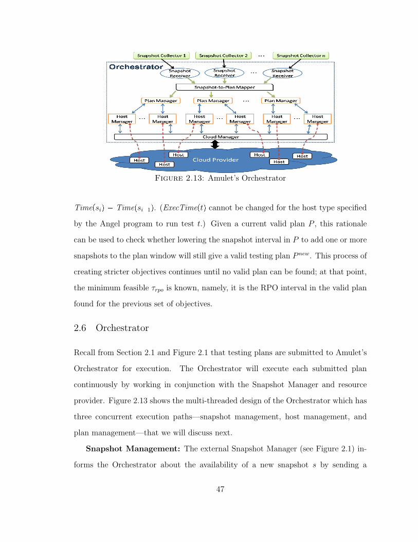
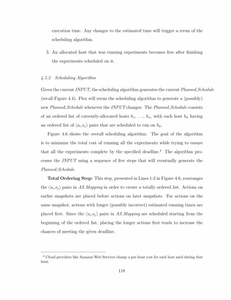
Figure 2.13: Amulet’s Orchestrator
Timepsiq � Timepsi�1q. (ExecTimeptq cannot be changed for the host type specified
by the Angel program to run test t.) Given a current valid plan P , this rationale
can be used to check whether lowering the snapshot interval in P to add one or more
snapshots to the plan window will still give a valid testing plan P new. This process of
creating stricter objectives continues until no valid plan can be found; at that point,
the minimum feasible τrpo is known, namely, it is the RPO interval in the valid plan
found for the previous set of objectives.
2.6 Orchestrator
Recall from Section 2.1 and Figure 2.1 that testing plans are submitted to Amulet’s
Orchestrator for execution. The Orchestrator will execute each submitted plan
continuously by working in conjunction with the Snapshot Manager and resource
provider. Figure 2.13 shows the multi-threaded design of the Orchestrator which has
three concurrent execution paths—snapshot management, host management, and
plan management—that we will discuss next.
Snapshot Management: The external Snapshot Manager (see Figure 2.1) in-
forms the Orchestrator about the availability of a new snapshot s by sending a
47
descriptor for s. Snapshots are never copied to the Orchestrator. Since s is at the
level of a volume V , the Plan Manager in charge of the testing plan for V is noti-
fied. In turn, the Host Managers responsible for hosts allocated to this plan from
the external resource provider get notified. Recall that the plan generated by the
Optimizer was based on PW
PIuniformly-spaced snapshots per plan window. The Plan
and Host Managers determine which snapshot in the window, if any, s should be
mapped to.
Host Management: A Host Manager is responsible for using and monitoring a
host allocated to a testing plan from the resource provider. Amulet’s implementation
supports any infrastructure-as-a-service cloud provider (e.g., Amazon Web Services,
Joyent, Rackspace) as the resource provider by using an appropriate Cloud Manager
(Figure 2.13). The Host Manager uses the API provided by the Cloud Manager to
allocate, establish connections with, and terminate hosts as well as to load snapshots
on to allocated hosts.
Plan Management: A Plan Manager is responsible for shepherding the execu-
tion of a testing plan P through one or more plan windows until P is terminated.
The Plan Manager’s role is straightforward at the conceptual level if P behaves as
the Optimizer estimated when P was generated. The challenge is when the Plan
Manager has to deal with unpredictable lags in the actual schedule of execution
from the Optimizer-estimated schedule, and with repair actions that need to be run
when corruption is detected.
Dealing with Lags: This process involves two steps: (i) identifying straggler hosts
on which the lag is observed; and (ii) allocating one or more helper hosts for each
straggler host subject to the reserved cost budget PR earmarked for the Orchestrator
to deal with unpredictable events. A testing host h is marked as a straggler when
two conditions hold:
48
1. The actual execution time of tests for a snapshot s on h has overshot the
corresponding estimated time by more than an allowed slack. (The slack is
used to prevent overreaction.) Straggler hosts are prioritized based on the age
of s.
2. The next snapshot s1 on which host h is scheduled to run tests has become
available.
Each helper host h1 for a straggler host h will take a share of h’s workload adap-
tively. The helper host h1 will be terminated if, on completing the execution of
tests on a snapshot, it is found that the corresponding testing host h is no longer a
straggler.
Handling Repairs: This process also involves two steps:
1. The first test t that detects a corruption on a snapshot s, and has an associated
repair action, will cause a repair host to be allocated to run the repair. Repairs
for any future tests that detect corruption on s will be run on the same host in
order to generate a single fully-repaired snapshot. Note that applying repairs
offers much less scope for parallel execution compared to running tests to detect
different types of corruption.
2. Once the repairs complete, a snapshot is taken to preserve the repaired version
of s, and the repair host is terminated.
When a new helper or repair host is needed, the Plan Manager checks whether it
has enough remaining budget from PR to allocate a new host. If not, the Plan Man-
ager will repeat the check at frequent intervals. In the worst case—e.g., if estimates
of test execution times from models were significantly lower than actual execution
times—an RPO or TCO objective will eventually get violated before a host can be
49
allocated. In that case, the Orchestrator will terminate the plan and send a notifi-
cation to the SA.
2.7 Experimental Evaluation
To the best of our knowledge, no other tool supports the functionality that Amulet
provides. So, we evaluated Amulet for correctness and we present a couple of use
cases along with insights from the developing and testing process.
2.7.1 Experimental Methodology and Setup
Methodology: We have implemented Amulet with all the components and al-
gorithms as described in the previous sections. We now present a comprehensive
evaluation of Amulet when run using the Amazon Web Services platform as the
infrastructure-as-a-service cloud provider. Section 2.7.2 considers the end-to-end ex-
ecution, with both optimization and orchestration, of Angel programs in Amulet. For
ease of exposition, we consider four scenarios that are simple in terms of Amulet’s
functionality, but illustrate the challenges that Amulet has to deal with. Amulet’s
power will become more clear in Section 2.7.3 where we consider both the efficiency
(how fast?) and effectiveness (how good is the selected plan?) of the Optimizer while
generating testing plans for huge plan spaces.
Database software stack and tests: For the production system, we choose a
popular database software stack composed of MySQL as the database system, XFS
or ext3 as the file-system, and Amazon’s Elastic Block Storage (EBS) volumes for
persistent storage (we used 50GB volumes) (Running MySQL on Amazon EC2 with
EBS). For each layer of the stack, we chose a representative test from Table 2.2:
myisamchk for MySQL database integrity checking, and fsck and xfs check for file-
system integrity checking. Execution-time estimation models for these tests were
trained and validated on the Amazon cloud (see Section 2.3).
50
Snapshots and storage: We implemented a Snapshot Manager that automates
periodic volume-level snapshots (currently, the only type supported by the Amazon
cloud). When the XFS file-system is used, the Snapshot Manager freezes the MySQL
database as well as the XFS file-system (all caches are flushed to the disk) before a
volume-level snapshot is taken (Running MySQL on Amazon EC2 with EBS). This
process finishes within seconds. For the ext3 file-system, only the database is frozen
since ext3 does not support the freeze feature of XFS.
Amazon provides two persistent storage services: Simple Storage Service (S3)
and Elastic Block Storage (EBS). EBS provides much faster data access rates than
S3, but has lower redundancy. Amazon supports snapshots of EBS volumes with
the caveat that these snapshots are stored in S3. Specifically, when the Snapshot
Manager initiates a snapshot, Amazon copies the EBS volume data to S3. All but
the first snapshot request to the same EBS volume will copy to S3 only the changed
data since the last snapshot.
Amazon does not provide direct access to data in a snapshot s. Instead, Amulet
can create an EBS volume from s, and attach this volume to a testing host h that
needs to run tests on s. This process copies data in a background fashion from the
snapshot stored in S3 to h—prioritizing block read/write requests from h—making
the volume accessible in h before the data movement is complete. Snapshot creation
and restore times depend on bandwidth constraints and the amount of data that
needs to be copied from S3 to EBS or EBS to S3. In our experiments, we observed
an average bandwidth of 20 MB/s in both directions. This process can be made
much faster by removing the intermediate copy to S3, which is part of our future
work.
Plan costs: Recall from Section 2.4.1 that a pricing model for the resource
provider has to be input to Amulet in order to specify cost objectives in Angel
programs. For evaluation purposes, we used a pricing model motivated by how
51
Table 2.8: Pricing model used in our evaluation
Resource Used Pay-as-you-go Pricing Method
Testing hostsHosts of the Small type (see Figure 2.4a) cost $0.085 per hour.Medium / Large types cost $0.17 / $0.34 per hour respectively
Storage $0.10 per month per 1 GB of persistent storage usedI/O to storage $0.10 per 1 million block I/O requests to persistent storageSnapshot access $0.05 per 1000 store or load requests for snapshots
Figure 2.14: Actual execution timeline on the Amazon Cloud for Case 2 in ourevaluation
resource usage is charged in a pay-as-you-go fashion on the Amazon cloud (Amazon
Web Services). Table 2.8 outlines this pricing model in terms of how the four main
types of resources used in a testing plan are charged. Given a testing plan P , Amulet’s
Optimizer will use the pricing model to find how much P ’s use of each resource will
cost in one plan window; and add all the per-resource costs to estimate P ’s total cost
per plan window. The total number of block I/O requests to persistent storage is
computed based on the total input data size for each test and the file-system’s block
size. This strategy was chosen based on our empirical observations. Enhancing each
test model to estimate the number of I/O requests that the test will make is part of
our future work.
2.7.2 End-to-End Processing of Angel Programs
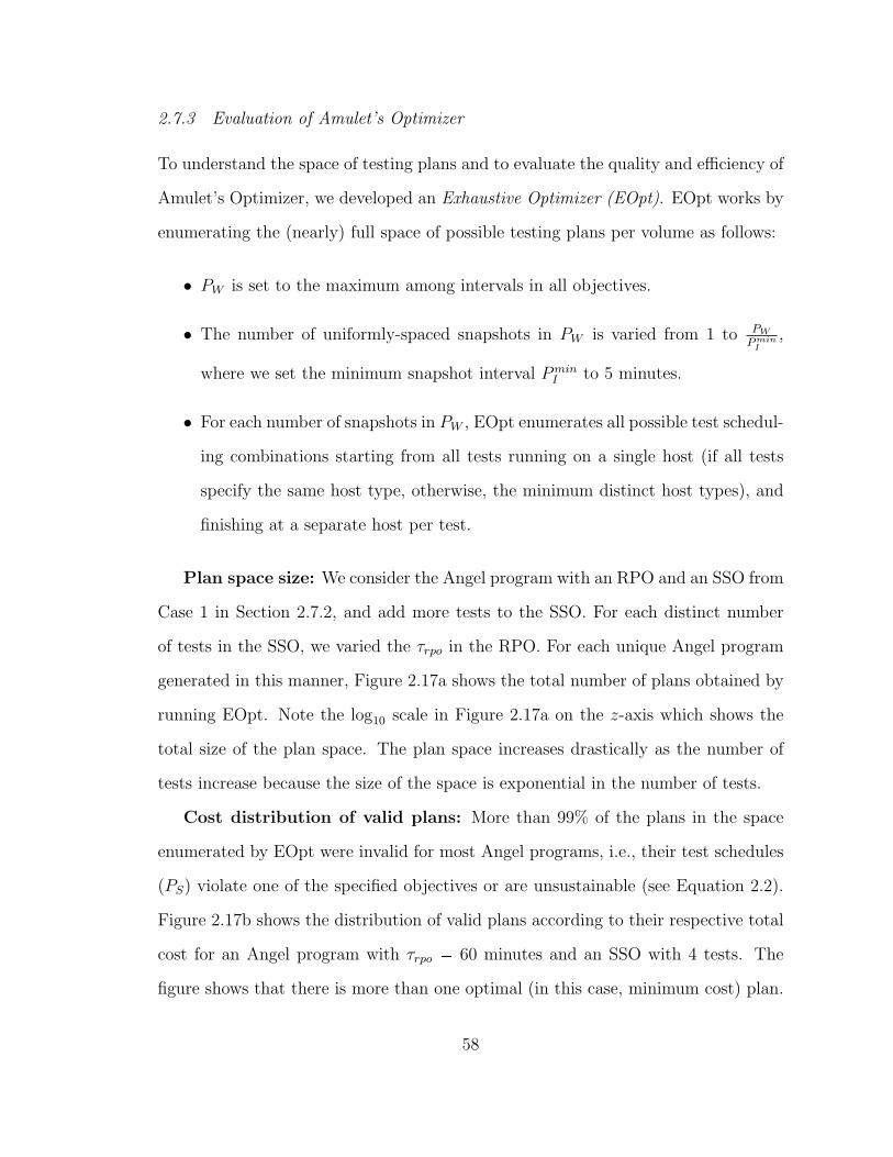
Case 1: Maintaining a Tested Recovery Point
Angel program: We first submit to Amulet the Angel program corresponding to
Example 1 from Table 2.5. The program specifies two objectives, an RPO and an
52
SSO, for a single volume. The time interval τrpo in the RPO is 60 minutes. The SSO
specifies a single test: a myisamchk medium test (denoted TM) on a database table
of size approximately 10 GB with no indexes. The test has to be run on hosts of
type Small (m1.small on the Amazon cloud). The Snapshot Manager sends snapshot
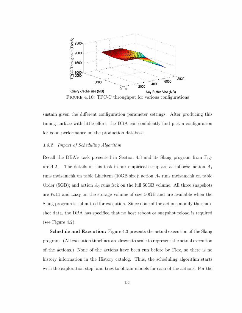
descriptors announcing new snapshots to Amulet every 15 minutes on average.
Testing Plan from the Optimizer: The model for estimating TM ’s execution
time returns an estimate of 20 minutes when invoked by the Optimizer for this setting.
The minimum-cost plan P generated by the Optimizer’s algorithm in Figure 2.7 for
this setting has:
• PI = 30 minutes
• PW = 60 minutes (PW
PI= 2 snapshots s1 and s2 per window)
• PM consists of test TM mapped to both snapshots in PW
• PS assigns one Small host to run TM on s1 and s2
• Since no CO is specified, PR takes the default value which in this case is the
cost of one Small host (see Section 2.4.1)
Orchestration Timeline: Figure 2.2 shows the actual execution timeline of
plan P when it is submitted to and run by the Orchestrator on the Amazon cloud.
The meaning of each important symbol used in the figure is described at the top.
The execution of P is shown for three plan windows, i.e., a total of 3 hours. When
P is submitted, the Orchestrator starts by requesting the needed testing host from
the cloud provider. When the host is available, the Orchestrator starts the plan
execution (0 minutes in the timeline in Figure 2.2).
The Orchestrator is continuously executing the schedule PS given by the Opti-
mizer for each plan window. As part of this process, the Orchestrator (actually the
53
Plan and Host Managers from Section 2.6) has to map the snapshots si, 1 ¤ i ¤PW
PI, identified by the Optimizer in the plan window to actual snapshots Sj collected
by the Snapshot Manager. Notice from Figure 2.2 that the Snapshot Manager is
submitting snapshot descriptors every 15 minutes on average, while the snapshot
interval PI in the plan is 30 minutes.
At Timepsiq, 1 ¤ i ¤ PW
PI, in the plan window, the Orchestrator checks whether a
snapshot S is available from the Snapshot Manager; if so, S will be tested. Otherwise,
the Orchestrator waits for a slack interval to see whether a new snapshot is submitted.
If no new snapshot arrives, then the last submitted snapshot will be tested. If this
snapshot has already been tested, then an error notification is generated. The Host
Manager uses PS to find out whether it has to load a submitted snapshot (and if so,
which tests it needs to run on the snapshot and how). Notice from Figure 2.2 that
every other snapshot submitted is tested. The boxes with notation SjTM in Figure 2.2
denote the actual run of test TM on snapshot Sj submitted by the Snapshot Manager.
The width of each box is the actual execution time of the test. These times are in
the 18-22 minutes range which matches the estimated execution time of 20 minutes.
Case 2: Multiple Tests and Multiple Objectives
Angel program: We now consider a more complex Angel program with more tests
as well as more and stricter objectives. The program specifies an RPO, an SSO,
and an SIO for a single volume. The time interval τrpo in the RPO is reduced to
30 minutes from before. The SSO specifies three tests: two myisamchk medium
tests respectively on a 2.4 GB lineitem table and a 1 GB orders table (with no
index on either table), and an fsck metadata test. All tests have to be run on Small
hosts. The SIO specifies Snapshot interval ¤ 10 minutes. The Snapshot Manager
sends snapshot descriptors announcing new snapshots to Amulet every 10 minutes
on average.
54
Testing Plan from the Optimizer: The minimum-cost plan P generated by
the Optimizer is more complex than before:
• PI = 10 minutes
• PW = 30 minutes (PW
PI= 3 snapshots s1, s2, s3 per window)
• PM has all three tests mapped to all three snapshots in PW
• PS assigns one host to run the fsck test (estimated to run in 6 minutes). The two
myisamchk tests are run concurrently on a second Small host, with estimated
times of 9 and 7 minutes.
• PR takes the default value as in Case 1
Orchestration Timeline: Figure 2.14 shows the actual execution timeline of
the above plan P . Note that PI = 10 minutes causes all submitted snapshots to be
tested. TML denotes the myisamchk test on lineitem, TMO denotes the myisamchk
test on orders, and TF denotes the fsck test. While there is some variance in the
actual execution times of the grouped test (1-2 minutes deviation from the estimates),
the plan works as the optimizer estimated.
Case 3: Dealing with Unpredictable Lags
Here we run the same Angel program as in Case 2. Thus, the same plan P is picked
and run as in Section 2.7.2. However, in this case, we cause a problem on Host1 which
causes the TML test on the host to run almost 2x slower than expected. Figure 2.15
shows the actual execution timeline.
Notice that test TML on snapshot S4 now takes around 16 minutes to run com-
pared to the estimated time of 9 minutes. The Plan Manager will mark Host1 as
a straggler because the two conditions for stragglers from Section 2.6 get satisfied
at around 52 minutes in the timeline. Host1 has overshot the estimated time, and
55
the next snapshot S5 on which Host1 has to run tests is ready. (A slack interval
of 2 minutes is used.) The Plan Manager will use the reserved cost budget PR to
request a helper host at time 52 minutes. The helper host is available at time 54
minutes, and takes over the running of the TML and TMO tests on snapshot S5 from
Host1. These tests complete at time 63. At that point, a check reveals that Host1
is no longer a straggler host; thus, the helper host is released back to the resource
provider. Intuitively, the helper host was pulled in adaptively to help the plan tide
over a transient problem.
Case 4: Corruption Detection and Repair
In this case, we cause a data corruption in the production system that manifests
itself in two snapshots. We create a scenario where a corruption happens due to
a software bug that does a misdirected write on the production system. We run
the Angel program from Case 2 with one change. The modified program associates
repair actions with the myisamchk tests on the lineitem and orders tables. The repair
actions invoke myisamchk with the “-r” option.
Figure 2.16 shows the actual execution timeline in this case. We inject the misdi-
rected write in the interval between 30 and 40 minutes in the timeline, which corrupts
the data in the lineitem table. Snapshots S4 and S5 submitted by the Snapshot Man-
ager contain this corruption. The corruption will be detected by TML when executed
on S4 (S4, TML in Figure 2.16). The corruption is reported to the Plan Manager
which uses the reserved cost budget PR to request a repair host. The repair action is
run on the repair host. When the repair finishes around time 60, a snapshot of the
repaired data is taken and the Snapshot Manager is notified. Around that time, the
Plan manager gets notified of the corruption detected in S5. The repair on S5 is run
on the same repair host, and the repaired snapshot is available at time 66. Since no
pending repairs exist at this point, the repair host is released.
56
��������� ������ ������ ������
������������
�������
����� �����������
�����������
���
��������
����� ��������� ������ ������ ������
����� ����� ���� ����� �����
����� ����� ����� �����
���
���
������������� ����� ���� ����� �����
�� �� �� �� �� ��
�����
���������� �� �� �� ��
���
����
���
��������
���������� �� �� �� ��
���
Figure 2.15: Actual execution timeline for Case 3
����� ��������� ������
������
������������
�����������
������ �����
��
� �� � �� � �� � �� � ��
������������
�������
���
����� ��� ���
����� ���
����� ����� ���� ����� �����
������ ������ ����� ������ ������
����
���
�� �� �� �� �� ��
����� �� �� �� �������
�����
����
���
��� �� �� �� �� �������
Figure 2.16: Actual execution timeline for Case 4
(a) Number of plans in the testing plan space
1 1.2 1.43 1.63 1.84 2.04 2.24 2.470
100
200
300
400
500
600
700
800
900
1000
1100
81
192
375
540
735
840
945 935
Plan Cost Relative to the Optimal Cost
Num
ber o
f Pla
ns
(b) Number of valid plans per price bucket
(c) Amulet Optimizer’s running time for costoptimization
(d) Amulet Optimizer’s running time for non-cost optimization
Figure 2.17: Characteristics of the testing plan space and the performance ofAmulet’s Optimizer
57
2.7.3 Evaluation of Amulet’s Optimizer
To understand the space of testing plans and to evaluate the quality and efficiency of
Amulet’s Optimizer, we developed an Exhaustive Optimizer (EOpt). EOpt works by
enumerating the (nearly) full space of possible testing plans per volume as follows:
• PW is set to the maximum among intervals in all objectives.
• The number of uniformly-spaced snapshots in PW is varied from 1 to PW
PminI
,
where we set the minimum snapshot interval PminI to 5 minutes.
• For each number of snapshots in PW , EOpt enumerates all possible test schedul-
ing combinations starting from all tests running on a single host (if all tests
specify the same host type, otherwise, the minimum distinct host types), and
finishing at a separate host per test.
Plan space size: We consider the Angel program with an RPO and an SSO from
Case 1 in Section 2.7.2, and add more tests to the SSO. For each distinct number
of tests in the SSO, we varied the τrpo in the RPO. For each unique Angel program
generated in this manner, Figure 2.17a shows the total number of plans obtained by
running EOpt. Note the log10 scale in Figure 2.17a on the z-axis which shows the
total size of the plan space. The plan space increases drastically as the number of
tests increase because the size of the space is exponential in the number of tests.
Cost distribution of valid plans: More than 99% of the plans in the space
enumerated by EOpt were invalid for most Angel programs, i.e., their test schedules
(PS) violate one of the specified objectives or are unsustainable (see Equation 2.2).
Figure 2.17b shows the distribution of valid plans according to their respective total
cost for an Angel program with τrpo � 60 minutes and an SSO with 4 tests. The
figure shows that there is more than one optimal (in this case, minimum cost) plan.
58
In this case—as well as in all cases where we could run EOpt in a reasonable time
frame—Amulet’s Optimizer generated one of the optimal plans.
Given the large plan space per volume and the speed at which it grows (Fig-
ure 2.17a), we measured the time that each optimizer takes to find a testing plan
per volume. We fixed τrpo to 60 minutes in the RPO, and varied the number of tests
in the SSO from 1 to 6. EOpt’s times increased rapidly from 0.5 seconds to 30+
minutes. (With 6 tests, we killed EOpt after 35 minutes.) Amulet’s Optimizer ran
in under 0.5 seconds in all these cases. We further increased the number of tests
up to 16 (which would be a high-end number for tests on a single volume). Our
Optimizer’s running time remained under 0.5 seconds.
Next, we increased the τrpo interval in the RPO, and specified an SIO with a
maximum snapshot interval of 1 minute to force our Optimizer to come up with a
plan where a snapshot is tested every minute. Figure 2.17c summarizes the results.
Planning for 3000 snapshots on each of which 16 tests should be run on average,
gave an Optimizer running time under 1 minute. We can see this result as: If the
snapshot interval PI is 5 minutes, then Amulet’s optimizer needs less than a minute
to produce a plan with a window PW spanning 10 days (3000 snapshots at PI=5
minutes per snapshot). We conclude that Amulet’s Optimizer is efficient for today’s
needs.
Finally, Figure 2.17d shows how Amulet’s Optimizer continues to remain efficient
even under non-cost optimization objectives. We used the binary-search algorithm
from Section 2.5.6 as the linear-search algorithm has a worse average case compared
to the binary-search. We defined a TCO and varied the time interval and the number
of tests that are part of the TCO. No cost objective was specified. The goal was to
maximize the number of tests in the plan. While non-cost optimization is more
expensive, the trend in Figure 2.17d is similar to what we observed for the cost
optimization objective in Figure 2.17c.
59
2.8 Conclusions and Future Work
Hardware errors, software bugs, and mistakes by human SAs can corrupt impor-
tant sources of data. Current approaches to deal with data corruption are ad hoc
and labor-intensive. We introduced the Amulet system that gives SAs a declarative
language to specify their objectives regarding the detection and repair of data cor-
ruption. Amulet automatically finds and orchestrates efficient testing plans that run
integrity tests to meet the specified objectives in cost-effective ways. We believe that
Amulet provides a general framework for SAs to analyze cost versus risk tradeoffs
regarding data protection. Although we prototyped Amulet on a cloud platform,
Amulet can be applied to conventional enterprise environments with minor modi-
fications. As future work we plan to explore several directions including adaptive
techniques for plan optimization.
60
3
Diagnosing with DiaDS
In this chapter, we present our contributions in the Diagnosing category, namely, a
tool called DiaDS. The main goal of DiaDS is to diagnose and find the root causes
of performance problems in multi-tier systems. This tool was evaluated and tested
on a Database System that runs on top of a Storage Area Network (SAN). Existing
diagnosis tools in this domain have a level-specific focus. Examples of such tools
include database-only diagnosis tools such as Dias et al. (2005) or SAN-only diagnosis
tools such as Shen et al. (2005).
DiaDS is a tool that carefully integrates information from several system layers,
including database and SAN systems (in our prototype implementation). The in-
tegration is not a simple concatenation of the monitoring data, but also includes
annotation of the monitoring data as well as attaching the relevant monitoring data
to the related system elements. This approach not only increases the accuracy of
diagnosis, but also leads to significant improvements in efficiency.
DiaDS uses a novel combination of non-intrusive machine learning techniques
(e.g., Kernel Density Estimation) and domain knowledge encoded in a new symp-
toms database design. The machine learning component provides core techniques for
61
problem diagnosis from monitoring data, and domain knowledge acts as checks-and-
balances to guide the diagnosis in the right direction. This unique system design
enables DiaDS to function effectively even in the presence of multiple concurrent
problems as well as noisy data prevalent in production environments. We present
the details of the implementation as well as the experimental evaluation in this chap-
ter.
3.1 Introduction
“The online transaction processing database myOLTP has a 30% slow down in pro-
cessing time, compared to performance two weeks back.” This is a typical problem
ticket a database administrator would create for the SAN administrator to analyze
and fix. Unless there is an obvious failure or degradation in the storage hardware or
the connectivity fabric, the response to this problem ticket would be: “The I/O rate
for myOLTP tablespace volumes has increased 40%, with increased sequential reads,
but the response time is within normal bounds.” This to-and-fro may continue for a
few weeks, often driving SAN administrators to take drastic steps such as migrating
the database volumes to a new isolated storage controller or creating a dedicated
SAN silo (the inverse of consolidation, explaining in part why large enterprises still
continue to have highly under-utilized storage systems). The myOLTP problem may
be fixed eventually by the database administrator realizing that a change in a table’s
properties had made the plan with sequential data scans inefficient; and the I/O
path was never an issue.
The above example is a realistic scenario from large enterprises with separate
teams of database and SAN administrators, where each team uses tools specific to
its own subsystem. With the growing popularity of Software-as-a-Service, this di-
vision is even more predominant with application administrators belonging to the
customer, while the computing infrastructure is provided and maintained by the ser-
62
SalesReports
[J2EE Enterprise Reporting Application]
SalesAppDB
[Postgres]
Query Query Query
Index Scan Table [ Product ]
Redhat Linux [Server]
WWN: 10000000C959F676
[HBA]
WWN: 1000000051E90550
[FCSwitch]
WWN: 1000000042D89053
[FCSwitch]
Fabric
Enterprise Class
[Storage Subsystem]
Pool2
[Storage Pool]
v4
[Storage Volume]
v1
[Storage Volume]
v2
[Storage Volume]
v3
[Storage Volume]
Pool1
[Storage Pool]
Disk
1
Disk
6
Disk
7
Disk
8
Disk
5
Disk
2
Disk
3
Disk
4
Record Fetch
Sort
Groupby
Index on Product.Price
Figure 3.1: Example database/SAN deployment.The dotted arrows indicate theeffect of noise in real-world data causing mis-classification of the root-cause
vice provider administrators. The result is a lack of end-to-end correlated informa-
tion across the system stack that makes problem diagnosis hard. Problem resolution
in such cases may require either throwing iron at the problem and re-creating re-
source silos, or employing highly-paid consultants who understand both databases
and SANs to solve the performance problem tickets.
The goal of this work is to develop an integrated diagnosis tool (called DiaDS)
that spans the database and the underlying SAN consisting of end-to-end I/O paths
63
Figure 3.2: Taxonomy of scenarios for root-cause analysis
with servers, interconnecting network switches and fabric, and storage controllers.
The input to DiaDS is a problem ticket from the SA with respect to a degradation
in database query performance. The output is a collection of top-K events from the
database and SAN that are candidate root causes for the performance degradation.
Internally, DiaDS analyzes thousands of entries in the performance and event logs of
the database and individual SAN devices to shortlist an extremely selective subset
for further analysis.
3.1.1 Challenges in Integrated Diagnosis
Figure 3.1 shows an integrated database and SAN taxonomy with various logical (e.g.,
sort and scan operators in a database query plan) and physical components (e.g.,
server, switch, and storage controller). Diagnosis of problems within the database
64
or SAN subsystem is an area of ongoing research (described later in Section 3.2).
Integrated diagnosis across multiple subsystems is even more challenging:
• High-dimensional search space: Integrated analysis involves a large num-
ber of entities and their combinations (see Figure 3.1). Pure machine learning
techniques that aim to find correlations in the raw monitoring data—which
may be effective within a single subsystem with few parameters—can be inef-
fective in the integrated scenario. Additionally, real-world monitoring data has
inaccuracies (i.e., the data is noisy). The typical source of noise is the large
monitoring interval (5 minutes or higher in production environments) which
averages out the instantaneous effects of spikes and other bursty behavior.
• Event cascading and impact analysis: The cause and effect of a problem
may not be contained within a single subsystem (i.e., event flooding may result).
Analyzing the impact of an event across multiple subsystems is a nontrivial
problem.
• Deficiencies of rule-based approaches: Existing diagnosis tools for some
commercial databases (e.g., Dias et al., 2005) use a rule-based approach where
a root-cause taxonomy is created and then complemented with rules to map
observed symptoms to possible root causes. While this approach has the merit
of encoding valuable domain knowledge for diagnosis purposes, it may become
complex to maintain and customize.
3.1.2 Contributions
The taxonomy of problem determination scenarios handled by DiaDS is shown in
Figure 3.2. The events in the SAN subsystem can be broadly classified into config-
uration changes (such as allocation of new applications, change in interconnectivity,
firmware upgrades, etc.) and component failure or saturation events. Similarly,
65
database events could correspond to changes in the configuration parameters of the
database, or a change in the workload characteristics driven by changes in query
plans, data properties, etc. The figure represents a matrix of change events, with rel-
atively complex scenarios arising due to combinations of SAN and database events.
In real-world systems, the no change category is misleading, since there will always
be change events recorded in management logs that may not be relevant or may not
impact the problem at hand; those events still need to be filtered by the problem de-
termination tool. For completeness, there is another dimension (outside the scope of
this work) representing transient effects, e.g., workload contention causing transient
saturation of components.
The key contributions of this work are:
• A novel workflow for integrated diagnosis that uses an end-to-end canonical
representation of database query operations combined with physical and logi-
cal entities from the SAN subsystem (referred to as dependency paths). DiaDS
generates these paths by analyzing system configuration data, performance
metrics, as well as event data generated by the system or by user-defined trig-
gers.
• The workflow is based on an innovative combination of machine learning, do-
main knowledge of configuration and events, and impact analysis on query
performance. This design enables DiaDS to address the integrated diagnosis
challenges of high-dimensional space, event propagation, multiple concurrent
problems, and noisy data.
• An empirical evaluation of DiaDS on a real-world testbed with a PostgreSQL
database running on an enterprise-class storage controller. We describe prob-
lem injection scenarios including combinations of events in the database and
SAN layers, along with a drill-down into intermediate results given by DiaDS.
66
3.2 Related Work
We give an overview of relevant database (DB), storage, and systems diagnosis work,
some of which is complementary and leveraged by our integrated approach.
3.2.1 Independent DB and Storage Diagnosis
There has been significant prior research in performance diagnosis and problem de-
termination in databases (e.g., Dias et al., 2005; Dageville et al., 2004; Mehta et al.,
2008) as well as enterprise storage systems (e.g., Pollack and Uttamchandani, 2006;
Shen et al., 2005). Most of these techniques perform diagnosis in an isolated manner
attempting to identify root cause(s) of a performance problem in individual database
or storage silos. In contrast, DiaDS analyzes and correlates data across the database
(Dageville et al., 2004; Dias et al., 2005) performs fine-grained monitoring to diag-
nose database performance problems, and to provide tuning recommendations. A
similar system (Chaudhuri et al., 2004) has been proposed for Microsoft SQLServer.
(Interested readers can refer to Weikum et al. (2002) for a survey on database prob-
lem diagnosis and self-tuning.) However, these tools are oblivious to the underlying
SAN layer. They cannot detect problems in the SAN, or identify storage-level root
causes that propagate to the database subsystem.
Storage-only Diagnosis: Similarly, there has been research in problem determi-
nation and diagnosis in enterprise storage systems. Genesis (Pollack and Uttam-
chandani, 2006) uses machine learning to identify abnormalities in SANs. A disk
I/O throughput model and statistical techniques to diagnose performance problems
in the storage layer are described in Shen et al. (2005). There has also been work
on profiling techniques for local file systems (e.g., Aranya et al., 2004; Zhou et al.,
67
1985) that help collect data useful in identifying performance bottlenecks as well as
in developing models of storage behavior (Joukov et al., 2006; Thereska et al., 2006;
Mesnier et al., 2007).
Drawbacks: Independent database and storage analysis can help diagnose prob-
lems like deadlocks or disk failures. However, independent analysis may fail to di-
agnose problems that do not violate conditions in any one layer, rather contribute
cumulatively to the overall poor performance. Two additional drawbacks exist. First,
it can involve multiple sets of experts and be time consuming. Second, it may lead
to spurious corrective actions as problems in one layer will often surface in another
layer. For example, slow I/O due to an incorrect storage volume placement may lead
a DB administrator to change the query plan. Conversely, a poor query plan that
causes a large number of I/Os may lead the storage administrator to provision more
storage bandwidth.
Studies measuring the impact of storage systems on database behavior (Reiss and
Kanungo, 2003; Qin et al., 2007) indicate a strong interdependence between the two
subsystems, highlighting the importance of an integrated diagnosis tool like DiaDS.
3.2.2 System Diagnosis Techniques
Diagnosing performance problems has been a popular research topic in the general
systems community in recent years (e.g., Wang et al., 2004; Cohen et al., 2004,
2005; Zhang et al., 2005; Basu et al., 2007; Manji). Broadly, this work can be split
into two categories: (a) systems using machine learning techniques, and (b) systems
using domain knowledge. As described later, DiaDS uses a novel mix where machine
learning provides the core diagnosis techniques while domain knowledge serves as
checks-and-balances against spurious correlations.
Diagnosis based on Machine Learning: PeerPressure (Wang et al., 2004) uses
statistical techniques to develop models for a healthy machine, and uses these models
68
to identify sick machines. Another proposed method (Basu et al., 2007) builds models
from process performance counters in order to identify anomalous processes that
cause computer slowdowns. There is also work on diagnosing problems in multi-tier
Web applications using machine learning techniques. For example, modified Bayesian
network models (Cohen et al., 2004) and ensembles of probabilistic models (Zhang
et al., 2005) that capture system behavior under changing conditions have been used.
These approaches treat data collected from each subsystem equally, in effect creating
a single table of performance metrics that is input to machine learning modules. In
contrast, DiaDS adds more structure and semantics to the collected data, e.g., to
better understand the impact of database operator performance vs. SAN volume
performance. Furthermore, DiaDS complements machine learning techniques with
domain knowledge.
Diagnosis based on Domain Knowledge: There are also many systems, espe-
cially in the DB community, where domain knowledge is used to create a symptoms
database that associates performance symptoms with underlying root causes (Yemini
et al., 1996; Manji; Perazolo, 2005; Dageville et al., 2004; Dias et al., 2005). Com-
mercial vendors like EMC, IBM, and Oracle use symptom databases for problem
diagnosis and correction. While these databases are created manually and require
expertise and resources to maintain, recent work attempts to partially automate this
process (Cohen et al., 2005; Duan et al., 2009a).
We believe that a suitable mix of machine learning techniques and domain knowl-
edge is required for a diagnosis tool to be useful in practice. Pure machine learning
techniques can be misled by spurious correlations in data resulting from noisy data
collection or event propagation (where a problem in one component impacts another
component). Such effects need to be addressed using appropriate domain knowl-
edge, e.g., component dependencies, symptoms databases, and knowledge of query
plan and operator relationships.
69
It is also important to differentiate DiaDS from tracing-based techniques (e.g.,
Chen et al., 2004; Aguilera et al., 2003) that trace messages through systems end-to-
end to identify performance problems and failures. Such tracing techniques require
changes in production system deployments and often add significant overhead in day-
to-day operations. In contrast, DiaDS performs a postmortem analysis of monitored
performance data collected at industry-standard intervals to identify performance
problems.
3.3 Overview of DiaDS
Suppose a query Q that a report-generation application issues periodically to the
database system shows a slowdown in performance. One approach to track down the
cause is to leverage historic monitoring data collected from the entire system. There
are several product offerings (e.g., EMC Control Center; Hewlett Packard Systems
Insight Manager; IBM Tivoli Network Manager; IBM TotalStorage Productivity Cen-
ter; VMWare Virtual Center) in the market that collect and persist monitoring data
from IT systems.
DiaDS uses a commercial storage management server – IBM TotalStorage Pro-
ductivity Center (IBM TotalStorage Productivity Center) – that collects monitoring
data from multiple layers of the IT stack including databases, servers, and the SAN.
The collected data is transformed into a tabular format, and persisted as time-series
data in a relational database.
SAN-level data: The collected data includes: (i) configuration of components
(both physical and logical), (ii) connectivity among components, (iii) changes in
configuration and connectivity information over time, (iv) performance metrics of
components, (v) system-generated events (e.g., disk failure, RAID rebuild) and (vi)
events generated by user-defined triggers (Garcia-Molina et al., 2001) (e.g., degrada-
tion in volume performance, high workload on storage subsystem).
70
Database-level data: To execute a query, a database system generates a plan
that consists of operators selected from a small, well-defined family of operators
(Garcia-Molina et al., 2001). Let us consider an example query Q:
SELECT Product.Category, SUM(Product.Sales)
FROM Product
WHERE Product.Price > 1000
GROUP BY Product.Category
Q asks for the total sales of products, priced above 1000, grouped per category.
Figure 3.1 shows a plan P to execute Q. P consists of four operators: an Index
Scan of the index on the Price attribute, a Fetch to bring matching records from
the Product table, a Sort to sort these records on Category values, and a Grouping
to do the grouping and summation. For each execution of P , DiaDS collects some
monitoring data per operator O. The relevant data includes: O’s start time, stop
time, and record-count (number of records returned in O’s output).
DiaDS’s Diagnosis Interface: DiaDS presents an interface where a SA can
mark a query as having experienced a slowdown. Furthermore, the SA either specifies
declaratively or marks directly the runs of the query that were satisfactory and those
that were unsatisfactory. For example, runs with running time below 100 seconds
are satisfactory, or all runs between 8 AM and 2 PM were satisfactory, and those
between 2 PM and 3 PM were unsatisfactory.
Diagnosis Workflow: DiaDS then invokes the workflow shown in Figure 3.3 to
diagnose the query slowdown based on the monitoring data collected for satisfactory
and unsatisfactory runs. By default, the workflow is run in a batch mode. However,
the SA can choose to run the workflow in an interactive mode where only one module
is run at a time. After seeing the results of each module, the SA can edit the data
or results before feeding them to the next module, bypass or reinvoke modules, or
stop the workflow.
71
Admin identifies instances of a query Q when it ran fine and when it did not
If plans are
different
Module PD: Look for changes in the plan used to execute Q when its
performance was satisfactory Vs. when performance was unsatisfactory
Same plan P involved in
good and bad performance
Plan−change analysis to pinpoint the cause
of plan changes (ex: index dropping, change in data
properties, change in configuration parameters, etc.)
Module CO: Correlate P’s slowdown with the running−time data of P’s operators
Module DA: Generate dependency paths for correlated operators from Module CO.
Prune the paths by correlating operator running times with component performance
Find causes with high confidence scores
Module SD: Match symptoms from Modules CR, CO, and
DA with symptoms database.
Module IA: For each high−confidence cause identified, find
Extract more symptoms
as needed by the database
how much of plan P’s slowdown can be explained by it
Module CR: Correlate P’s slowdown
with record−count data of P’s operators
Query
Plans
Operators
Components
Events
Symptoms
Impact
Figure 3.3: DiaDS’s diagnosis workflow
The first module in the workflow, called Module Plan-Diffing (PD), looks for
significant changes between the plans used in satisfactory and unsatisfactory runs. If
such changes exist, then DiaDS tries to pinpoint the cause of the plan changes (which
includes, e.g., index addition or dropping, changes in data properties, or changes in
configuration parameters used during plan selection).
The remaining modules are invoked if DiaDS finds a plan P that is involved in
both satisfactory and unsatisfactory runs of the query. We give a brief overview
before diving into the details in Section 3.4:
• Module Correlated Operators (CO): DiaDS finds the (nonempty) sub-
set of operators in P whose change in performance correlates with the query
slowdown. The operators in this subset are called correlated operators.
72
• Module Dependency Analysis (DA): Having identified the correlated op-
erators, DiaDS uses a combination of correlation analysis and the configuration
and connectivity information collected during monitoring to identify the com-
ponents in the system whose performance is correlated with the performance
of the correlated operators.
• Module Correlated Record-counts (CR): Next, DiaDS checks whether the
change in P ’s performance is correlated with the record-counts of P ’s operators.
If significant correlations exist, then it means that data properties have changed
between satisfactory and unsatisfactory runs of P .
• Module Symptoms Database (SD): The correlations identified so far are
likely symptoms of the root cause(s) of query slowdown. Other symptoms
may be present in the stream of system-generated events and trigger-generated
(user-defined) semantic events. The combination of these symptoms is used
to probe a symptoms database that maps symptoms to the underlying root
cause(s). The symptoms database improves diagnosis accuracy by dealing with
the propagation of faults across components as well as missing symptoms, un-
expected symptoms (e.g., spurious correlations), and multiple simultaneous
problems.
• Module Impact Analysis (IA): The symptoms database computes a confi-
dence score for each suspected root cause. For each high-confidence root cause
R, DiaDS performs impact analysis to answer the following question: if R is
really a cause of the query slowdown, then what fraction of the query slow-
down can be attributed to R. To the best of our knowledge, DiaDS is the first
automated diagnosis tool to have an impact-analysis module.
73
Integrated database/SAN diagnosis: Note that the workflow “drills down”
progressively from the level of the query to plans and to operators, and then uses
dependency analysis and the symptoms database to further drill down to the level
of performance metrics and events in components. Finally, impact analysis is a “roll
up” to tie potential root causes back to their impact on the query slowdown. The
drill down and roll up are based on a careful integration of information from the
database and SAN layers; and is not a simple concatenation of database-only and
SAN-only modules. Only low overhead monitoring data is used in the entire process.
Machine learning + domain knowledge: DiaDS’s workflow is a novel com-
bination of elements from machine learning with the use of domain knowledge. A
number of modules in the workflow use correlation analysis which is implemented
using machine learning; the details are in Sections 3.4.1 and 3.4.2. Domain knowl-
edge is incorporated into the workflow in Modules DA, SD, and IA; the details are
given respectively in Section 3.4.2–3.4.4. As we will demonstrate, the combination
of machine learning and domain knowledge provides built-in checks and balances to
deal with the challenges listed in Section 3.1.
3.4 Modules in the Workflow
We now provide details for all modules in DiaDS’s diagnosis workflow. Upfront, we
would like to point out that our main goal is to describe an end-to-end instantiation
of the workflow. We expect that the specific implementation techniques used for the
modules will change with time as we gain more experience with DiaDS.
3.4.1 Identifying Correlated Operators
Objective: Given a plan P that is involved in both satisfactory and unsatisfactory
runs of the query, DiaDS’s objective in this module is to find the set of correlated
operators. Let O1, O2, . . . , On be the set of all operators in P . The correlated
74
operators form the subset of O1, . . . , On whose change in running time best explains
the change in P ’s running time (i.e., P ’s slowdown).
Technique: DiaDS identifies the correlated operators by analyzing the monitor-
ing data collected during satisfactory and unsatisfactory runs of P . This data can
be seen as records with attributes A, tpP q, tpO1q, tpO2q, . . . , tpOnq for each run of P .
Here, attribute tpP q is the total time for one complete run of P , and attribute tpOiqis the running time of operator Oi for that run. Attribute A is an annotation (or
label) associated with each record that represents whether the corresponding run of
P was satisfactory or not. Thus, A takes one of two values: satisfactory (denoted S)
or unsatisfactory (denoted U).
Let the values of attribute tpOiq in records with annotation S be s1, s2, . . . , sk,
and those with annotation U be u1, u2, . . . , ul. That is, s1, . . . , sk are k observations
of the running time of operator Oi when the plan P ran satisfactorily. Similarly,
u1, u2, . . . , ul are l observations of the running time of Oi when the running time of
P was unsatisfactory. DiaDS pinpoints correlated operators by characterizing how
the distribution of s1, . . . , sk differs from that of u1, . . . , ul. For this purpose, DiaDS
uses Kernel Density Estimation (KDE) (Parzen, 1962).
KDE is a non-parametric technique to estimate the probability density function
of a random variable. Let Si be the random variable that represents the running
time of operator Oi when the overall plan performance is satisfactory. KDE applies a
kernel density estimator to the k observations s1, . . . , sk of Si to learn Si’s probability
density function fipSiq.
fipSiq �°kj�1KpSi�sj
hq
kh(3.1)
Here, K is a kernel function and h is a smoothing parameter. A typical kernel is
75
the standard Gaussian function Kpxq � e�x2
2?2π
. (Intuitively, kernel density estimators
are a generalization and improvement over histograms.)
Let u be an observation of operator Oi’s running time when the plan performance
was unsatisfactory. Consider the probability estimate probpSi ¤ uq � ³u�8 fipSiqdsi.
Intuitively, as u becomes higher than the typical range of values of Si, probpSi ¤ uqbecomes closer to 1. Thus, a high value of probpSi ¤ uq represents a significant
increase in the running time of operator Oi when plan performance was unsatisfactory
compared to that when plan performance was satisfactory.
Specifically, DiaDS includes Oi in the set of correlated operators if probpSi ¤uq ¥ 1 � α. Here, u is the average of u1, . . . , ul and α is a small positive constant.
α � 0.1 by default. For obvious reasons, probpSi ¤ uq is called the anomaly score of
operator Oi.
3.4.2 Dependency Analysis
Objective: This module takes the set of correlated operators as input, and finds
the set of system components that show a change in performance correlating with
the change in running time of one of more correlated operators.
Technique: DiaDS implements this module using dependency analysis which is
based on generating and pruning dependency paths for the correlated operators. We
describe the generation and pruning of dependency paths in turn.
Generating dependency paths: The dependency path of an operator Oi is the set
of physical (e.g., server CPU, database buffer cache, disk) and logical (e.g., volume,
external workload) components in the system whose performance can have an impact
on Oi’s performance. DiaDS generates dependency paths automatically based on the
following data:
76
1. System-wide configuration and connectivity data as well as updates to this
data collected during the execution of each operator (recall Section 3.3).
2. Domain knowledge of how each database operator executes. For example, the
dependency path of a sort operator that creates temporary tables on disk will
be different from one that does not create temporaries.
We distinguish between inner and outer dependency paths. The performance
of components in Oi’s inner dependency path can affect Oi’s performance directly.
Oi’s outer dependency path consists of components that affect Oi’s performance
indirectly by affecting the performance of components on the inner dependency path.
As an example, the inner dependency path for the Index Scan operator in Figure 3.1
includes the server, HBA, FCSwitches, Pool2, Volume v2, and Disks 5-8. The outer
dependency path will include Volumes v1 and v3 (because of the shared disks) and
other database queries.
Pruning dependency paths: The fact that a component C is in the dependency
path of an operator Oi does not necessarily mean that Oi’s performance has been
affected by C’s performance. After generating the dependency paths conservatively,
DiaDS prunes these paths based on correlation analysis using KDE.
Recall from Section 3.3 that the monitoring data collected by DiaDS contains
multiple observations of the running time of operator Oi both when the overall plan
ran satisfactorily and when the plan ran unsatisfactorily. For each run of Oi, consider
the performance data collected by DiaDS for each component C in Oi’s dependency
path; this data is collected in the rtb, tes time interval where tb and te are respectively
Oi’s (absolute) start and stop times for that run. Across all runs, this data can
be represented as a table with attributes A, tpOiq,m1, . . . ,mp. Here, m1-mp are
performance metrics of component C, and the annotation attribute A represents
whether Oi’s running time tpOiq was satisfactory or not in the corresponding run.
77
It follows from Section 3.4.1 that we can set A’s value in a record to U (denoting
unsatisfactory) if probpSi ¤ tpOiqq ¥ 1� α; and to S otherwise.
Given the above annotated performance data for an xOi, Cy operator-component
pairing, we can apply correlation analysis using KDE to identify C’s performance
metrics that are correlated with the change in Oi’s performance. The details are
similar to that in Section 3.4.1 except for the following: for some performance metrics,
observed values lower than the typical range are anomalous. This correlation can
be captured using the condition probpM ¤ vq ¤ α, where M is the random variable
corresponding to the metric, v is a value observed for M , and α is a small positive
constant.
In effect, the dependency analysis module will identify the set of components
that: (i) are part of Oi’s dependency path, and (ii) have at least one performance
metric that is correlated with the running time of a correlated operator Oi. By
default, DiaDS will only consider the components in the inner dependency paths of
correlated operators. However, components in the outer dependency paths will be
considered if required by the symptoms database (Module SD).
Recall Module CR in the diagnosis workflow where DiaDS checks for significant
correlation between plan P ’s running time and the record counts of P ’s operators.
DiaDS implements this module using KDE in a manner almost similar to the use of
KDE in dependency analysis; hence Module CR is not discussed further.
3.4.3 Symptoms Database
The modules so far in the workflow drilled down from the level of the query to that of
physical and logical components in the system; in the process identifying correlated
operators and performance metrics. While this information is useful, the detected
correlations may only be symptoms of the true root cause(s) of the query slowdown.
This issue, which can mask the true root cause(s), is generally referred to as the event
78
(fault) propagation problem in diagnosis. For example, a change in data properties
at the database level may, in turn, propagate to the volume level causing volume
contention, and to the server level increasing CPU utilization. In addition, some
spurious correlations may creep in and manifest themselves as unexpected symptoms
in spite of our careful drill down process.
Objective: DiaDS’s Module SD tries to map the observed symptoms to the
actual root cause(s), while dealing with missing as well as unexpected symptoms
arising from the noisy nature of production systems.
Technique: DiaDS uses a symptoms database to do the mapping. This database
streamlines the use of domain knowledge in the diagnosis workflow to:
• Generate more accurate diagnosis results by dealing with event propagation.
• Generate diagnosis results that are semantically more meaningful to SAs (for
example, reporting lock contention as the root cause instead of reporting some
correlated metrics only).
We considered a number of formats proposed previously in the literature to input
domain knowledge for aiding diagnosis. Our evaluation criteria were the following:
I. How easy is the format for SAs to use? Here, usage includes customization,
maintenance over time, as well as debugging. When a diagnosis tool pinpoints
a particular cause, it is important that the SAs are able to understand and
validate the tool’s reasoning. Otherwise, SAs may never trust the tool enough
to use it.
II. Can the format deal with the noisy conditions in production systems, including
multiple simultaneous problems, presence of spurious correlations, and missing
symptoms.
79
symp2
symp1
symp3
symp4
1R
2R
3R
1 1
1
111
0
0 0
0
1 0
Figure 3.4: Example codebook
One of the formats from the literature (IBM Tivoli Network Manager) is an
expert knowledge-base of rules where each rule expresses patterns or relationships
that describe symptoms, and can be matched against the monitoring data. Most of
the focus in this work has been on exact matches, so this format scores poorly on
Criterion II. Representing relationships among symptoms (e.g., event X will cause
event Y ) using deterministic or probabilistic networks like Bayesian networks (Pearl,
2000) has been gaining currency recently. This format has high expressive power,
but remains a black-box for SAs who find it hard to interpret the reasoning process
(Criterion I).
Another format, called the Codebook (Yemini et al., 1996), is very intuitive as
well as implemented in a commercial product. This format assumes a finite set of
symptoms such that each distinct root cause R has a unique signature in this set.
That is, there is a unique subset of symptoms that R gives rise to which differs makes
it distinguishable from all other root causes. This information is represented in the
Codebook which is a matrix whose columns correspond to the symptoms and rows
correspond to the root causes. A cell is mapped to 1 if the corresponding root cause
should show the corresponding symptom; and to 0 otherwise. Figure 3.4 shows an
example Codebook where there are four hypothetical symptoms symp1–symp4 and
three root causes R1–R3.
When presented with a vector V of symptoms seen in the system, the Codebook
computes the distance dpV,Rq of V to each row R (i.e., root cause). Any number
of different distance metrics can be used, e.g., Euclidean (L2) distance or Hamming
80
distance (Yemini et al., 1996). dpV,Rq is a measure of the confidence that R is a
root cause of the problem. For example, given a symptoms vector x1, 0, 0, 1y (i.e.,
only symp1 and symp4 are seen), the Euclidean distances to the three root causes in
Figure 3.4 are 0,?
2, and 1 respectively. Hence, R1 is the best match.
The Codebook format does well on both our evaluation criteria. Codebooks can
handle noisy situations, and SAs can easily validate the reasoning process. However,
DiaDS needs to consider complex symptoms such as symptoms with temporal prop-
erties. For example, we may need to specify a symptom where a disk failure is seen
within X minutes of the first incidence of the query slowdown, where X may vary
depending on the installation. Thus, it is almost impossible in our domain to fully
enumerate a closed space of relevant symptoms, and to specify for each root cause
whether each symptom from this space will be seen or not. These observations led
to DiaDS’s new design of the symptoms database:
1. We define a base set of symptoms consisting of: (i) operators in the database
system that can be included in the correlated set, (ii) performance metrics
of components that can be correlated with operator performance, and (iii)
system-monitored and user-defined events collected by DiaDS.
2. The language defined by IBM’s Active Correlation Technology (ACT) is used
to express complex symptoms over the base set of symptoms (Biazetti and
Gajda, 2005). The benefit of this language comes from its support for a range of
built-in patterns including filter, collection, duplicate, computation, threshold,
sequence, and timer. ACT can express symptoms like: (i) the workload on a
volume is higher than 200 IOPS, and (ii) event E1 should follow event E2 in
the 30 minutes preceding the first instance of query slowdown.
3. DiaDS’s symptoms database is a collection of root cause entries each of which
has the format Cond1 & Cond2 & . . . & Condz, for some z ¡ 0 which can differ
81
across entries. Each Condi is a Boolean condition of the form Dsympj (denoting
presence of sympj) or Dsympj (denoting absence of sympj). Here, sympj is
some base or complex symptom. Each Condi is associated with a weight wi
such the sum of the weights for each individual root cause entry is 100%. That
is,°zi�1wi � 100%.
4. Given a vector of base symptoms, DiaDS computes a confidence score for each
root cause entry R as the sum of the weights of R’s conditions that evaluate
to true. Thus, the confidence score for R is a value in r0%, 100%s equal to°zi�1wi|Condi � true.
DiaDS’s symptoms database tries to balance the expressive power of rules with
the intuitive structure and robustness of Codebooks. The symptoms database differs
from conventional Codebooks in a number of ways. For each root cause entry, DiaDS
avoids the “closed-world” assumption for symptoms by mapping symptoms to 0, 1, or
“don’t care”. Conventional Codebooks are constrained to 0 or 1 mappings. DiaDS’s
symptoms database can contain mappings for fixes to problems in addition to root
causes. This feature is useful because it may be easier to specify a fix for a query
slowdown (e.g., add an index) instead of trying to find the root cause. DiaDS also
allows multiple distinct entries for the same root cause.
Generation of the symptoms database: Companies like EMC, IBM, HP,
and Oracle are investing significant (currently, mostly manual) effort to create symp-
toms databases for different subsystems like networking infrastructure, application
servers, and databases (Yemini et al., 1996; Manji; Perazolo, 2005; Cohen et al.,
2005; Dageville et al., 2004; Dias et al., 2005). Symptoms databases created by some
of these efforts are already in commercial use. The creation of these databases can
be partially automated, e.g., through a combination of fault injection and machine
learning (Cohen et al., 2005; Duan et al., 2009a). In fact, DiaDS’s modules like corre-
82
lation, dependency, and impact analysis can be used to identify important symptoms
automatically.
3.4.4 Impact Analysis
Objective: The confidence score computed by the symptoms database module for
a potential root cause R captures how well the symptoms seen in the system match
the expected symptoms of R. For each root cause R whose confidence score exceeds
a threshold, the impact analysis module computes R’s impact score. If R is an actual
root cause, then R’s impact score represents the fraction of the query slowdown that
can be attributed to R individually. DiaDS’s novel impact analysis module serves
three significant purposes:
• When multiple problems coexist in the system, impact analysis can separate
out high-impact causes from the less significant ones; enabling prioritization of
SA effort in problem solving.
• As a safeguard against misdiagnoses caused by spurious correlations due to
noise.
• As an extra check to find whether we have identified the right cause(s) or all
cause(s).
Technique: Interestingly, one approach for impact analysis is to invert the pro-
cess of dependency analysis from Section 3.4.2. Let R be a potential root cause
whose impact score needs to be estimated:
1. Identify the set of components, denoted comppRq, that R affects in the inner
dependency path of the operators in the query plan. DiaDS gets this informa-
tion from the symptoms database.
83
2. For each component C P comppRq, find the subset of correlated operators,
denoted oppRq, such that for each operator O in this subset: (i) C is in O’s
inner dependency path, and (ii) at least one performance metric of C is corre-
lated with the change in O’s performance. DiaDS has already computed this
information in the dependency analysis module.
3. R’s impact score is the percentage of the change in plan running time (query
slowdown) that can be attributed to the change in running time of operators
in oppRq. Here, change in running time is computed as the difference between
the average running times when performance is unsatisfactory and that when
performance is satisfactory.
The above approach will work as long as for any pair of suspected root causes R1
and R2, oppR1q X oppR2q � H. However, if there are one or more operators common
to oppR1q and oppR2q whose running times have changed significantly, then the above
approach cannot fully separate out the individual impacts of R1 and R2.
DiaDS addresses the above problem by leveraging plan cost models that play a
critical role in all database systems. For each query submitted to a database system,
the system will consider a number of different plans, use the plan cost model to
predict the running time (or some other cost metric) of each plan, and then select
the plan with minimum predicted running time to run the query to completion.
These cost models have two main components:
• Analytical formula per operator type (e.g., sort, index scan) that estimates
the resource usage (e.g., CPU and I/O) of the operator based on the values of
input parameters. While the number and types of input parameters depend
on the operator type, the main ones are the sizes of the input processed by the
operator.
84
• Mapping parameters that convert resource-usage estimates into running-time
estimates. For example, IBM DB2 uses two such parameters to convert the
number of estimated I/Os into a running-time estimate: (i) the overhead per
I/O operation, and (ii) the transfer rate of the underlying storage device.
The following are two examples of how DiaDS uses plan cost models:
• Since DiaDS collects the old and new record-counts for each operator, it es-
timates the impact score of a change in data properties by plugging the new
record-counts into the plan cost model.
• When volume contention is caused by an external workload, DiaDS estimates
the new I/O latency of the volume from actual observations or the use of device
performance models. The impact score of the volume contention is computed
by plugging this new estimate into the plan cost model.
DiaDS’s use of plan cost models is a general technique for impact analysis, but it
is limited by what effects are accounted for in the model. For example, if wait times
for locks are not modeled, then the impact score cannot be computed for locking-
based problems. Addressing this issue—e.g., by extending plan cost models or by
using planned experiments at run time—is an interesting avenue for future work.
3.5 Experimental Evaluation
The taxonomy of scenarios considered for diagnosis in the evaluation follows from
Figure 3.2. DiaDS was used to diagnose query slowdowns caused by (i) events within
the database and the SAN layers, (ii) combinations of events across both layers, as
well as (iii) multiple concurrent problems (a capability unique to DiaDS). Due to
space limitations, it is not possible to describe all the scenario permutations from
Figure 3.2. Instead, we start with a scenario and make it increasingly complex by
85
combining events across the database and SAN. We consider: (i) volume contention
caused by SAN misconfiguration, (ii) database-level problems (change in data prop-
erties, contention due to table locking) whose symptoms propagate to the SAN, and
(iii) independent and concurrent database-level and SAN-level problems.
We provide insights into how DiaDS diagnoses these problems by drilling down
to the intermediate results like anomaly, confidence, and impact scores. While there
is no equivalent tool available for comparison with DiaDS, we provide insights on the
results that a database-only or SAN-only tool would have generated; these insights
are derived from hands-on experience with multiple in-house and commercial tools
used by SAs today. Within the context of the scenarios, we also report sensitivity
analysis of the anomaly score to the number of historic samples and length of the
monitoring interval.
3.5.1 Setup Details
Our experimental testbed is part of a production SAN environment, with the inter-
connecting fabric and storage controllers being shared by other applications. Our
experiments ran during low activity time-periods on the production environment.
The testbed runs data-warehousing queries from the popular TPC-H benchmark
(tpch, 2009) on a PostgreSQL database server configured to access tables using two
Ext3 filesystem volumes created on an enterprise-class IBM DS6000 storage con-
troller. The database server is a 2-way 1.7 GHz IBM xSeries machine running Linux
(Redhat 4.0 Server), connected to the storage controller via Fibre Channel (FC) host
bus adaptor (HBA). Both the storage volumes are RAID 5 configurations consisting
of (4 + 2P) 15K FC disks.
An IBM TotalStorage Productivity Center (IBM TotalStorage Productivity Cen-
ter) SAN management server runs on a separate machine recording configuration
details, statistics, and events from the SAN as well as from PostgreSQL (which was
86
instrumented to report the data to the management tool). Figure 3.6 shows the key
performance metrics collected from the database and SAN. The monitoring data is
stored as time-series data in a DB2 database. Each module in DiaDS’s workflow is
implemented using a combination of Matlab scripts (for KDE) and Java. DiaDS uses
a symptoms database that was developed in-house to diagnose query slowdowns in
database over SAN deployments.
Our experimental results focus on the slowdown of the plan shown in Figure 3.5
for Query 2 from TPC-H. Figure 3.5 shows the 25 operators in the plan, denoted
O1–O25. In database terminology, the operators Index Scan and Sequential Scan are
leaf operators since they access data directly from the tables; hence the leaf operators
are the most sensitive to changes in SAN performance. The plan has 9 leaf operators.
The other operators process intermediate results.
3.5.2 Scenario 1: Volume Contention due to SAN Misconfiguration
Problem Setting
In this scenario, a contention is created in volume V1 (from Figure 3.5) causing a
slowdown in query performance. The root cause of the contention is another appli-
cation workload that is configured in the SAN to use a volume V’ that gets mapped
to the same physical disks as V1. For an accurate diagnosis result, DiaDS needs to
pinpoint the combination of SAN configuration events generated on: (i) creation of
the new volume V’, and (ii) creation of a new zoning and mapping relationship of
the server running the workload that accesses V’.
Module CO
DiaDS analyzes the historic monitoring samples collected for each of the 25 query
operators. The monitoring samples for an operator are labeled as satisfactory or
unsatisfactory based on past problem reports from the SA. Using the operator run-
87
Figure 3.5: Query plan, operators, and dependency paths for the experimentalresults
ning times in these labeled samples, Module CO in the workflow uses KDE to com-
pute anomaly scores for the operators (recall Section 3.4.1). Table 3.1 shows the
anomaly scores of the operators identified as the correlated operators; these opera-
tors have anomaly scores ¥ 0.8 (the significance of the anomaly scores is covered in
Section 3.4.1). The following observations can be made from Table 3.1:
88
Database Metrics Server Metrics Network Metrics Storage Metrics
Operator Start Stop Times
Record-counts
Plan Start Stop Times
Locks outstanding and
held
Lock wait times Space Usage
Blocks Read
Buffer Hits
Index Scans
Index Reads Index Fetches
Sequential Scans
CPU Usage (%ge)
CPU Usage (Mhz)
Handles
Threads
Processes
Heap Memory Usage(KB) Physical Memory Usage (%)
Kernel Memory(KB)
Memory Being Swapped(KB)
Reserved Memory
Capacity(KB) Wait I/O
Network Bandwidth (HBA)
Bytes Transmitted
Bytes Received
Packets Transmitted
Packets Received
LIP Count NOS Count
Error Frames
Dumped Frames
Link Failures
CRC Errors Address Errors
Bytes Read
Bytes Written
Contaminating Writes
PhysicalStorageRead Operations
Physical Storage Read Time PhysicalStorageWriteOperations
Physical Storage Write Time
Sequential Read Requests
Sequential Write Requests
Total IOs
Figure 3.6: Important performance metrics collected by DiaDS
• Leaf operators O8 and O22 were correctly identified as correlated. These two
are the only leaf operators that access data on the Volume V1 under contention.
• Eight intermediate operators were ranked highly as well. This ranking can be
explained by event propagation where the running times of these operators are
affected by the running times of the “upstream” operators in the plan (in this
case O8 and O22).
• A false positive for leaf operator O4 which operates on tables in Volume V2.
This could be a result of noisy monitoring data associated with the operator.
In summary, Module CO’s KDE analysis has zero false negatives and one false
positive from the total set of 9 leaf operators. The false positive gets filtered out
later in the symptoms database and impact analysis modules.
To further understand the anomaly scores, we conducted a series of sensitivity
tests. Figure 3.7 shows the sensitivity of the anomaly scores of three representative
operators to the number of samples available from the satisfactory runs. O22’s score
converges quickly to 1 because O22’s running time under volume contention is almost
5X the normal. However, the scores for leaf operator O11 and intermediate operator
O1 take around 20 samples to converge. With fewer than these many samples, O11
could have become a false positive. In all our results, the anomaly scores of all
89
Table 3.1: Anomaly scores for query operators from Figure 3.5 in Scenario 1
Figure 3.7: Sensitivity of anomaly scores to the number of satisfactory samples.While O22 shows highly anomalous behavior, scores for O1 and O11 should be low
25 operators converge within 20 samples. While more samples may be required in
environments with higher noise levels, the relative simplicity of KDE (compared to
models like Bayesian networks) keeps this number low.
Figure 3.8 shows the sensitivity of O22’s anomaly score to the length of the mon-
itoring interval during a 4-hour period. Intuitively, larger monitoring intervals sup-
press the effect of spikes and bursty access patterns. In our experiments, the query
running time was around 4 minutes under satisfactory conditions. Thus, monitoring
intervals of 10 minutes and larger in Figure 3.8 cause the anomaly score to deviate
more and more from the true value.
90
5min(48) 10min(24)20min(12) 40min(6) 80min(3)0
0.10.20.30.40.50.60.70.80.9
1
Time Interval(Number of samples)
An
om
aly
sco
re
Figure 3.8: Sensitivity of anomaly scores to noise in the monitoring data
Table 3.2: Anomaly scores computed during dependency analysis for performancemetrics from Volumes V1, V2
Volume, Anomaly Score Anomaly ScorePerf. Metric (no contention in V2) (contention in V2)V1, writeIO 0.894 0.894
V1, writeTime 0.823 0.823V2, writeIO 0.063 0.512
V2, writeTime 0.479 0.879
Module DA
This module generates and prunes dependency paths for correlated operators in order
to relate operator performance to database and SAN component performance. For
ease of presentation, we will focus on the leaf operators in Figure 3.5 since they are
the most sensitive to SAN performance. Given the configuration of our experimental
testbed in Figure 3.5, the primary difference between the dependency paths of various
operators is in the volumes they access: V1 is in the dependency path of O8 and O22,
and V2 is in the paths of O4, O11, O14, O16, O19, O23, and O25.
The set of correlated operators from Module CO are O4, O8, and O22. Thus,
DiaDS will compute anomaly scores for the performance metrics of both V1 and V2.
Table 3.2’s second column shows the anomaly scores for two representative metrics
each from V1 and V2. (Table 3.2’s third column is described later in this section.)
As expected, none of V2’s metrics are identified as correlated because V2 has no
contention; while those of V1 are.
91
Module CR
Anomaly scores are low in this module because data properties do not change.
Module SD
The symptoms identified up to this stage are:
• High anomaly scores for operators dependent on V1.
• High anomaly scores for V1’s performance metrics.
• High anomaly score for only one V2-dependent operator (out of seven such
operators).
These symptoms are strong evidence that V1’s performance is a cause of the query
slowdown, and V2’s performance is not. Thus, even when a symptoms database is
not available, DiaDS correctly narrows down the search space a SA has to consider
during diagnosis. An impact analysis will further point out that the false positive
symptom due to O4 has little impact on the query slowdown.
However, without a symptoms database or further diagnosis effort from the SA,
the root cause of V1’s change of performance is still unknown among possible candi-
dates like: (i) change of performance of an external workload, (ii) a runaway query
in the database, or (iii) a RAID rebuild. We will now report results from the use
of a symptoms database that was developed in-house. DiaDS uses this database
as described in Section 3.4.3 except that instead of reporting numeric confidence
scores to SAs, DiaDS reports confidence as one of High (score ¥ 80%), Medium
(80% ¡ score ¥ 50%), or Low (50% ¡ score ¥ 0%). The summary of Module SD’s
output in the current scenario is:
• All root causes with contention-related symptoms for V2 have Low confidence
(few symptoms are found).
92
• RAID rebuild gets Low confidence because no RAID rebuild start or end events
are found.
• V1 contention due to changes in data properties gets Low confidence because
symptoms are missing.
• V1 contention due to change in external workload gets Low confidence because
no external workload was on the outer dependency path of a correlated operator
when performance was satisfactory.
• V1 contention due to change in database workload gets Medium confidence
because of a weak correlation between the performance of some correlated
operators and the rest of the database workload.
• V1 contention due to the SAN misconfiguration problem gets High confidence
because all specified symptoms are found including: (i) creation of a new vol-
ume (parametrized with the physical disk information), and (ii) creation of new
masking and zoning information for the volume.
The symptoms database had an entry for the actual root cause because this
problem is common. Hence, DiaDS was able to diagnose the root cause for this
scenario. Note that DiaDS had to consider more than 900 events (system generated
as well as user-defined) for the database and SAN generated during the course of the
satisfactory and unsatisfactory runs for this experiment.
Module IA
Impact analysis done using the inverse dependency analysis technique gives an impact
score of 99.8% for the high-confidence root cause found. This score is high because
the slowdown is caused entirely by the contention in V1.
93
In keeping with our experimental methodology, we complicated the problem sce-
nario to test DiaDS’s robustness. Everything was kept the same except that we
created extra I/O load on Volume V2 in a bursty manner such that this extra load
had little impact on the query beyond the original impact of V1’s contention. With-
out intrusive tracing, it would not be possible to rule out the extra load on V2 as a
potential cause of the slowdown.
Interestingly, DiaDS’s integrated approach is still able to give the right answer.
Compared to the previous scenario, there will now be some extra symptoms due to
higher anomaly scores for V2’s performance metrics (as shown in the third column
in Table 3.2). However, root causes with contention-related symptoms for V2 will
still have Low confidence because most of the leaf operators depending on V2 will
have low anomaly scores as before. Also, impact scores will be low for these causes.
Unlike DiaDS, a SAN-only diagnosis tool may spot higher I/O loads in both V1
and V2, and attribute both of these as potential root causes. Even worse, the tool
may give more importance to V2 because most of the data is on V2. A database-only
tool can pinpoint the slowdown in the operators. However, this tool cannot track the
root cause down to the SAN level because it has no visibility into SAN configuration
or performance. From our experience, database-only tools may give several false
positives in this context, e.g., suboptimal bufferpool setting or a suboptimal choice
of execution plan.
3.5.3 Scenario 2: Database-Layer Problem Propagating to the SAN-Layer
In this scenario we cause a query slowdown by changing the properties of the data,
causing extra I/O on Volume V2. The change is done by an update statement that
modifies the value of an attribute in some records of the part table. The overall size of
all tables, including part, are unchanged. There are no external causes of contention
on the volumes.
94
Modules CO, DA, and CR behave as expected. In particular, module CR cor-
rectly identifies all the operators whose record-counts show a correlation with plan
performance: operators O1, O2, O3, and O4 show increased record-counts, while op-
erators O5 and O6 show reduced record-counts. The root-cause entry for changes
in data properties gets High confidence in Module SD because all needed symptoms
match. All other root-cause entries get Low confidence, including contention due
to changes in external workload and database workload because no correlations are
detected on the outer dependency paths of correlated operators (as expected).
The impact analysis module gives the final confirmation that the change in data
properties is the root cause, and rules out the presence of high-impact external causes
of volume contention. As described in Section 3.4.4, we can use the plan cost model
from the database to estimate the individual impact of any change in data properties.
In this case, the impact score for the change in data properties is 88.31%. Hence,
DiaDS could have diagnosed the root cause of this problem even if the symptoms
database was unavailable or incomplete.
3.5.4 Scenario 3: Concurrent Database-Layer and SAN-Layer Problems
We complicate Scenario 2 by injecting contention on Volume V2 due to SAN miscon-
figuration along with the change in data properties. Both these problems individually
cause contention in V2. The SAN misconfiguration is the higher-impact cause in our
testbed. This key scenario represents the occurrence of multiple, possibly related,
events at the database and SAN layers, complicating the diagnosis process. The
expected result from DiaDS is the ability to pinpoint both these events as causes,
and giving the relative impact of each cause on query performance.
The CO, DA, and CR Modules behave in a fashion similar to Scenario 2, and
drill down to the contention in Volume V2. We considered DiaDS’s performance in
two cases: with and without the symptoms database. When the symptoms database
95
is unavailable or incomplete, DiaDS cannot distinguish between Scenarios 2 and
3. However, DiaDS’s impact analysis module computes the impact score for the
change in data properties, which comes to 0.56%. (This low score is representative
because the SAN misconfiguration has more than 10X higher impact on the query
performance than the change in data properties.) Hence, DiaDS final answer in this
case is as follows: (i) a change in data properties is a high-confidence but low-impact
cause of the problem, and (ii) there are one or more other causes that impact V2
which could not be diagnosed.
When the symptoms database is present, both the actual root causes are given
High confidence by Module SD because the needed symptoms are seen in both cases.
Thus, DiaDS will pinpoint both the causes. Furthermore, impact analysis will con-
firm that the full impact on the query performance can be explained by these two
causes.
A database-only diagnosis tool would have successfully diagnosed the change in
data properties in both Scenarios 2 and 3. However, the tool may have difficulty
distinguishing between these two scenarios or pinpointing causes at the SAN layer.
A SAN-only diagnosis tool will pinpoint the volume overload. However, it will not
be able to separate out the impacts of the two causes. Since the sizes of the tables
do not change, we also suspect that such a tool may even rule out the possibility of
a change in data properties being a cause.
3.5.5 Discussion
The scenarios described in the experimental evaluation were carefully chosen to be
simple, but not simplistic. They are representative of event categories occurring
within the DB and SAN layers as shown in Figure 3.2. We have additionally ex-
perimented with different events within those categories such as CPU and memory
contention in the SAN in addition to disk-level saturation, different types of database
96
misconfiguration, and locking-based database problems. Locking-based problems are
hard to diagnose because they can cause different types of symptoms in the SAN
layer, including contention as well as underutilization. We have also considered con-
current occurrence of three or more problems, e.g., change in data properties, SAN
misconfiguration, and locking-based problems. The insights from these experiments
are similar to those seen already, and further confirm the utility of an integrated
tool. However:
• High levels of noise in the monitoring data can reduce DiaDS’s effectiveness.
• While DiaDS would still be effective when the symptoms database is incom-
plete, more manual effort will be needed to pinpoint actual root causes.
• Incomplete or inaccurate plan cost models reduce the accuracy of impact anal-
ysis.
3.6 Conclusions and Future Work
This chapter presented an integrated database and storage diagnosis tool called Di-
aDS. Using a novel combination of machine learning techniques with database and
storage expert domain-knowledge, DiaDS accurately identifies the root cause(s) of
problems in query performance; irrespective of whether the problem occurs in the
database or the storage layer. This integration enables a more accurate and effi-
cient diagnosis tool for SAs. Through a detailed experimental evaluation, we also
demonstrated the robustness of our approach: with its ability to deal with multiple
concurrent problems as well as the presence of noisy data.
In future, we are interested in exploring two directions of research. First, we are
investigating approaches that further strengthen the analysis done as part of DiaDS
modules, e.g., techniques that complement database query plan models using planned
97
run-time experiments. Second, we aim to generalize our diagnosis techniques to
support applications other than databases in conjunction with enterprise storage.
98
4
Testing with Flex
In this chapter we present our contributions in the Testing category, namely, a system
called Flex. Flex is motivated by the routine need from the SAs to perform testing of
productions systems with production-like workloads (W ), configurations (C), data
(D), and resources (R). The further W , C, D, and R used in testing and tuning
deviate from what is observed on the production database instance, the lower is the
trustworthiness of the testing and tuning tasks done. For example, it is common
to hear about performance degradations observed after the production system is
upgraded from one software version to another. A typical cause of this problem is
that the W , C, D, or R used during upgrade testing differed in some way from that
on the production database. Performing testing and tuning tasks in principled and
automated ways is very important, especially since—spurred by innovations in cloud
computing—the number of systems that a SA has to manage is growing rapidly.
Flex is a platform for trustworthy testing and tuning of production systems. To
make the presentation concrete, we present the integration of Flex with production
database system instances. Flex gives DataBase Administrators (DBAs) a declara-
tive language, called Slang, to specify definitions and objectives regarding running
99
experiments for testing and tuning. Flex’s orchestrator schedules and runs these
experiments in an automated manner that meets the DBA-specified objectives. In
this chapter, we present the implementation as well as results from a comprehensive
empirical evaluation that reveals the effectiveness of Flex on diverse problems such
as upgrade testing, near-real-time testing to detect corruption of data, and server
configuration tuning.
4.1 Introduction
It is estimated that, over the next decade, the number of servers (virtual and physical)
in enterprise datacenters will grow by a factor of 10, the amount of data managed by
these datacenters will grow by a factor of 50, and the number of files the datacenter
has to deal with will grow by a factor of 75 (Digital Universe, 2011). Meanwhile,
skilled information technology (IT) staff to manage the growing number of servers
and data will increase less than 1.5 times (Digital Universe, 2011).
The implication of this trend is clear. The days where a database administrator
(DBA) is responsible for managing one or few production database instances are
numbered. In the near future, a DBA will be responsible for the administration
of tens to hundreds of database instances. The DBA will need to ensure that the
production databases, each serving real applications and users, are available 24x7,
and that the databases perform as per specified requirements. We are already starting
to see very high database-to-DBA ratios in pioneering companies like Salesforce.
High database-to-DBA ratios are only possible through extensive automation of
database administration. Automation of tasks like database installation and moni-
toring has seen major advances. Significant progress has also been made towards
automating administrative tasks like backups, failover, defragmentation, index re-
builds, and patch installation (e.g., Elmore et al., 2011; Oracle Online Index Re-
build). However, more challenging administrative tasks to meet database availabil-
100
ity and performance goals are harder to automate. We will first give examples of
problems that have often happened in practice, and will continue to happen unless
new solutions are developed.
Upgrade problems: Consider an upgrade of the database software from one
version to another. The database developers will run standard test suites to test the
new version. However, when a customer upgrades her production database instance
to the new version, a performance degradation is experienced. Many instances of this
problem are documented for database systems such as MySQL (Peter Zaitsev, 2007),
Oracle (Oracle Upgrade Regression), PostgreSQL (PostgreSQL TPC-H Bug), and
others. Typically, some unique characteristic of the production instance—e.g., the
scale or correlations in the production data, the properties of the production server
hardware or operating environment, or mix of queries in the production workload—
causes the problem to manifest during production use but not during offline testing.
Tuning problems: A production database instance will need to be tuned when
it is not meeting specified performance requirements. A DBA’s usual course of action
is to try to replicate the production environment in a test setting. The DBA would
then run and monitor parts of the workload on the test database instance to recreate
the problem, narrow down its possible causes, and identify a fix for the problem.
A highly nontrivial next step is to estimate whether the fix will actually solve the
performance problem on the production database instance; multiple trial-and-error
steps may be needed. Well-meaning changes to production instances have led to
performance or availability problems in the past (CouchDB Data Loss, 2010).
Data integrity problems: Corruption of data is a serious problem where bits of
data stored in persistent storage differ from what they are supposed to be (Borisov
et al., 2011). Data corruption can lead to three undesirable outcomes: data loss,
system unavailability, and incorrect results. Such problems have been caused in
production database instances due to hardware problems such as errors in magnetic
101
media (bit rot), bit flips in CPU or RAM due to alpha particles, bugs in software or
firmware, as well as mistakes by human administrators (Subramanian et al., 2010).
It took only one unfortunate instance of data corruption (which spread from the
production instance to backups), and the consequent loss of data stored by users, to
put a popular social-bookmarking site out of business (Magnolia, 2009).
The above problems indicate the need to test and tune the production database
instance in an efficient and timely fashion with production-like workloads (W ), con-
figurations (C), data (D), and hardware and software resources (R). The further W ,
C, D, and R deviate from what is observed in the production instance, the lower is
the trustworthiness of the testing and tuning tasks done.
At the same time, the interactions of the testing and tuning tasks with the produc-
tion database instance have to be managed carefully. First, the performance overhead
on the production instance must be minimal. Thus, the resources used for testing
and tuning have to be well isolated from those used by the production database in-
stance to serve real applications and users. Second, the impact of potential changes
recommended for the production instance have to be verified as thoroughly as pos-
sible before they are actually made. These challenges are nontrivial partly because
an automated solution is needed to handle the scale where a single DBA manages
hundreds of production database instances. The Flex platform is designed to address
these challenges.
Table 4.1: Listing of some nontrivial uses enabled by the Flex platform. W ptq, Cptq, Dptq,and Rptq respectively denote the respective states of the workload, configuration, data, andresources for the production database instance at time t
A/B testingDescription of databaseadministration task inEnglish
How would the current database workload have performedif index I1 had (hypothetically) been part of the productiondatabase’s configuration?
Continued on next page
102
Task specification usingw,c,r,d representation
Run experiment e = xw=W ptcurq,c,r=Rptcurq,d=Dptcurqy,where c=CptcurqYtI1u, and compare the observed per-formance with the production database’s performance onits current workload W ptcurq, configuration Cptcurq, dataDptcurq, and resources Rptcurq
Things to note Tries a configuration different from the production database’scurrent one
Tuning surface creation (Figure 4.10)Description of databaseadministration task inEnglish
How does the throughput obtained for my website’s OLTPworkload due to my MySQL database change as itsquery cache size and key buffer size parameters are varied inthe ranges [0,10GB] and [0,8GB] respectively?
Task specification usingw,c,r,d representation
For qiP[0,10GB] & kjP[0,8GB], run experiment eij =xw=W ptcurq,cij ,r=Rptcurq,d=Dptcurqy, where cij is Cptcurqwith two changes: parameter query cache size is set to qiand key buffer size is set to kj
Things to note Gives potential to run multiple independent experiments inparallel
Upgrade planningDescription of databaseadministration task inEnglish
Suppose my production PostgreSQL database was runningthe newer version 9.0 instead of the current version 8.4.Would any performance regression have been observed forthe workload and data from 10.00 AM of each day of lastweek as well as each day of the coming week?
Task specification usingw,c,r,d representation
For time tP 24 hour increments from [6/1/2012,10AM]to [6/14/2012,10AM], run experiment ei = xw=W ptq,c �Cptq,ri,d=Dptqy, where ri has the same hardware charac-teristics as Rptq, but runs the newer database software 9.0instead of 8.4 in order to find the performance difference
Things to note Tries a different software image on the production database’spast and future states
Data integrity testingDescription of databaseadministration task inEnglish
A security patch was applied to my production Oracle DB.The patch could cause data corruption. Run Oracle’s DB-verify corruption detection tool on the Lineitem and Ordertables once every hour. (Alert if corruption is detected)
Task specification usingw,c,r,d representation
For time t in 1 hour increments starting now, run experimente = xw,c=Cptq,r=Rptq,d=Dptqy, where w is the DBverifytool run on the Lineitem and Order tables
Things to note Runs a custom workload on an indefinite number of futurestates
Stress testingDescription of databaseadministration task inEnglish
If the workload on my production database goes up by 10xin the coming holiday season, then how will it perform?
Task specification usingw,c,r,d representation
Run experiment e = xw,c=Cptcurq,r=Rptcurq,d=Dptcurqy,where w is W ptcurq scaled by a factor of 10
Things to note Uses a scaled version of workload1
End of Table 4.1
103
4.1.1 Flex
The Flex platform enables efficient experimentation for trustworthy testing and tun-
ing of production database instances. Figure 4.1 gives a high-level illustration of the
core concepts that Flex is based on. These concepts will be defined precisely later
in the chapter.
Flex treats the production database instance as an entity that can evolve over
time. As illustrated in Figure 4.1, this entity is represented in terms of the workload
W on the database, the configuration C (such as indexes and configuration param-
eters) of the database, the data D in the database, and the resources R (such as
server hardware and software image) used by the database. Since each of W , C, D,
and R can change over time, we will use W ptq, Cptq, Dptq, and Rptq to denote their
respective point-in-time states at time t.
For testing or tuning the production database instance, a DBA can ask Flex to
run one or more experiments. An experiment e = xw,c,r,dy starts a database instance
on resources r with configuration c and data d, and runs workload w. As illustrated
in Figure 4.1, Flex enables w, c, r, and d to be derived directly from the state of
the production database instance at a specific time in the past, current, or future;
or they can come from a custom specification.
Table 4.1 gives a number of nontrivial tasks that can be achieved by the DBA
through experiments using Flex. Flex will run each specified experiment automat-
ically and efficiently. Flex ensures that the resources r used in any experiment are
well isolated from the resources used by the production database instance. Multi-
ple experiments can be run in parallel subject to the DBA’s objectives regarding
experiment completion times and number of usable hosts.
Figure 4.1: Overview of how Flex enables trustworthy experimentation with state(workload, configuration, and data) derived from the production database instance
4.1.2 Contributions and Challenges
Slang declarative language: The first challenge in Flex is to develop a language
in which DBAs or higher-level services can express a wide spectrum of experiment-
driven administrative tasks like those illustrated in Table 4.1. We have developed
the Slang2 declarative language that supports the key abstractions needed to specify
such tasks easily and intuitively. In addition, Slang enables users and services to
specify objectives on the number of hosts and completion times that Flex should
meet while running the experiments. Section 4.2 and Section 4.4 describe Slang and
its abstractions.
Orchestration of experiments: Given a Slang program, Flex automates the
entire orchestration from planning and execution of the program, to run-time moni-
toring and adaptation. The orchestration process has to address multiple challenges
in order to run the needed experiments while meeting the objectives specified:
1 Similar experiments can be done in Flex with scaled data sizes.2 The name slang came from Fl{ex lang}uage.
105
• How much resources to allocate for running the experiments?
• In what order to schedule the experiments on these resources?
• How to efficiently load data needed for experiments from the production database
instance on to the allocated resources?
We have developed a novel technique for orchestration in Flex that uses a mix of
exploration (to learn models to predict experiment running times) and exploitation
(use of the learned models for planning) to meet the objectives in the Slang program.
This technique is both elastic (it can grow and shrink its resource usage) and adaptive
(it can react as unforeseen events such as failures arise or new information such as
experiment running times is available). Flex also supports a number of different
techniques to transfer evolving data from the production database instance to the
resources allocated to run experiments. The details of the orchestration techniques
are presented in Section 4.5 and Section 4.6.
Prototype system: We have implemented the full set of language and system
features in a prototype of Flex where the production database instance and experi-
ments all run on a cloud platform such as Amazon Web Services (AWS), Rackspace,
or SQL Azure. Cloud platforms are an excellent fit for Flex because these platforms
are leading the massive growth in the use of compute and storage resources and the
accompanying increase in database-to-DBA ratios. Furthermore, Flex is designed
to take advantage of the elastic and pay-as-you-go nature of cloud platforms. The
architecture and implementation of Flex are presented in Section 4.7.
Section 4.8 presents results from a comprehensive empirical evaluation of the
Flex platform. We demonstrate how Flex simplifies and improves the effectiveness
of upgrade testing, production database tuning, and data integrity testing. We have
taken a testing application from the literature and ported it to run on Flex as a
106
Flex Service. We dive into the details in order to demonstrate the ease of developing
higher-level testing and tuning applications using Flex. We also give a comparison
of this service when it runs on Flex versus when it runs as written originally.
4.2 Abstraction of an Experiment
Intuitively, a replica of the production database instance has to be created in order
to run an experiment. Three steps are involved in order to run an experiment:
• Identifying—with the possibility of having to provision dynamically—a host h
that will provide the resources to run the experiment.3
• Loading a snapshot s of some specific state from the production database in-
stance on to the selected host h.
• Running an action a associated with the experiment on the combination of the
host h and snapshot s.
In this fashion, an experiment in Flex is represented as e = xa,s,hy. The rest of
this section will elaborate on the three steps listed above, and also clarify how the
xa,s,hy representation subsumes the xw,c,d,ry representation from Section 4.1.
Host: In this work, we consider database instances that run on a single (possibly
multicore) server. These instances are similar to the main database server product
sold by most commercial database vendors as well as popular open-source databases
like MySQL and PostgreSQL. (Extending Flex to support parallel database instances
is an interesting avenue for future work which is discussed in Section 4.10.) A host
in Flex is a server that can run a database instance as part of an experiment. Flex
associates two types of information with a host: the underlying server’s hardware
characteristics as well as the software image that runs on the server.
3 It is inadvisable to run experiments on the production database instance since the experimentscould cause unpredictable behavior.
107
A host can be represented in a number of ways, and Flex can adopt any one
of these. We have chosen to use a simple methodology that is motivated by how
cloud providers represent hosts. The host’s hardware resources are represented by a
host type. As an example, AWS’s Elastic Compute Cloud (EC2) supports thirteen
different host types currently (Amazon Host Types). Each host type maps to a
specification of resources that will be contained in any host allocated of that type.
For example, AWS’s default m1.small type is a 32-bit host with 1.7 GB memory, 1
EC2 Compute Unit, and 160 GB local storage with moderate I/O performance.
The software that runs on a host is represented by an image. Each software image
has a unique identifier that represents the combination of software components in
that image such as the OS, file-system, and database management system. For
example, an image on AWS comes with pre-configured OS and application software
that is started when a host is allocated. Most database vendors provide images to
run their database software on EC2 hosts.
Snapshot: A snapshot is a point-in-time representation of the entire state of a
database system. A snapshot collection process that runs on the production database
instance generates a snapshot whenever one is needed. This snapshot collection
process—we give the details of one in Section 4.6—may also ensure that the snapshots
are made persistent on a local or remote storage volume. Three types of state are
captured in a snapshot:
• The actual data (D) stored in the database.
• The database configuration (C) which includes information such as indexes and
materialized views, the database catalog, and server configuration parameters
such as buffer pool settings.
• The database workload (W ) in the form of logs such as SQL query logs and
Figure 4.2: Example slang program #1 that references past snapshots
Thus, a snapshot captures the data D, configuration C, and workload W in the
production database instance at a point of time. The snapshot needed by one or more
experiments has to be transferred to the host allocated to run these experiments. Flex
manages this transfer efficiently as we will describe in Section 4.6.
Action: To run an experiment e = xa,s,hy, Flex will load the snapshot s on
to the host h, and then run the action a. The action a can be specified as a new
user-defined executable or from a library of commonly-used actions. As illustrated
in Table 4.1, the following are some commonly-used actions in experiments that Flex
runs:
• Replay the workload as captured in the snapshot s (Galanis et al., 2008).
• Update the existing configuration by building a new index or changing one or
more server configuration parameters, and then replay the SQL query workload.
• Run a custom workload such as a corruption detection tool or a scaled version
of the workload logged in the snapshot s.
109
����������
���� �
�������������� ����������
�����
� �������
������������
���� �
�����������
����
����������
���� �
���� �
�����
����� ���� �
����������������
���� �� ���� �
�����������
���� � ���������������� ���������������
�� �� �� �� �� �� �� �� ��!�"��
����
#"��$
Figure 4.3: Execution of example slang program #1 from Figure 4.2 (Section 4.8.2gives a detailed description)
4.3 Walk-through of Flex Usage
We will begin with a walk-through of how Flex is used for a specific task by a human
user such as a DBA or a database developer. (The “user” here can also be a Flex
Service for automated testing or tuning.) The task is expressed in English as: Verify
the data integrity of the three collected snapshots—snap-1, snap-2, and snap-3—by
running the myisamchk tool on the Lineitem and Order tables as well as the fsck tool
on the file-system. Complete this task within 90 minutes. Use m1.small hosts on
Amazon Web Services and do not use more than 3 hosts concurrently.
Example Slang program #1 in Figure 4.2 shows how the user will express this
task in the Slang declarative language. Broadly speaking, Slang provides support
for: (i) definitions of actions, snapshots, and hosts; (ii) mappings that stitch the
definitions together into each one of the experiments that needs to be run; (iii) and
the objectives that should be met while running the experiments.
Flex will parse the input Slang program and do some semantic checks. The ex-
tracted definitions, mappings, and objectives are given to Flex’s Orchestrator which
coordinates the scheduling, execution, and monitoring of experiments. Figure 4.3
shows the complete execution timeline of the example Slang program #1 from Fig-
ure 4.2. Notice from Figure 4.3 that the Orchestrator has to make choices regarding
when to allocate and release hosts, which experiments to schedule on which hosts
110
Table 4.2: Summary of statements in the Slang language
Statement Description
Action Definition of an action a, namely, the executable for a, the data a operateson, and (possibly) setup/cleanup scripts
Host Host definition used to specify the resources to request and access fromthe resource provider
Credentials Access definitions for Flex to use and request resources from the resourceprovider
Plan Provides mapping between actions and snapshots (specifying the completeaction-snapshot-resource mapping is an optional feature aimed at expertusers)
Snapshot Snapshot specification along with incoming arrival rates
and when (which, in turn, determines which snapshots are loaded on which hosts),
and how to deal with unpredictable events that can arise during the execution.
Three hosts—Host1, Host2, and Host3—were allocated in Figure 4.3. The figure
shows the beginning and end times of each experiment on the respective host where
the experiment was scheduled. In this schedule, snapshots snap-1 and snap-2 are
loaded on all hosts, while snapshot snap-3 is loaded only on Host1. Note that,
in order to minimize concurrent resource usage, while meeting the deadline, Flex
released two hosts midway through the execution.
All the snapshots needed in our example task came from past states of the pro-
duction database instance. Recall from Table 4.1 that Slang programs may also need
to refer to future snapshots. These snapshots will be processed by Flex when they
arrive. In this case, the orchestration behaves like the execution of continuous queries
over streams of data, as we will illustrate later in the chapter.
4.4 Slang Language
All inputs to Flex are specified in Slang. It is natural to ask why a new language
had to be developed for Flex. For example, couldn’t Flex use an existing workflow
definition language (e.g., BPEL, 2011)? To the best of our knowledge, no existing
111
language achieves a good balance between: (i) being powerful enough to express
a wide variety of experimentation needs such as the use cases in Table 4.1, and
(ii) being simple enough for humans to use and for extracting information needed
for automatic optimization. Our approach to achieve this balance was to come up
with the right abstractions in Slang. These abstractions are represented by the five
statements summarized in Table 4.2 and described next.
Action: Each unique type of action a involved in an experiment e = xa,s,hy is
defined by an Action statement. The execute and datum clauses in the statement
specify respectively the executable that needs to be run for a and the data on which
a operates. The Action statement enables additional requirements and properties to
be specified for a such as: (i) the host h needs to be restarted before a is executed;
(ii) a modifies the data that it operates on; (iii) a model to estimate the expected
execution time of a; and (iv) a specific host type that a should be executed on.
For example, in Figure 4.2, action A1 specifies the use of the myisamchk1.sh exe-
cutable (which invokes MySQL’s myisamchk corruption detection tool) operating on
the Lineitem table. The statement specifies that A1 does not modify the data and
that the host need not be rebooted before A1 is invoked. The statement also spec-
ifies two executables that are respectively invoked before (e.g., for starting custom
monitoring tools) and after (e.g., for some cleanup) the action’s execution.
Host: Each unique type of host involved in an experiment e = xa,s,hy is defined
by a Host statement. As discussed in Section 4.2, the Host statement specifies two
identifiers: one for the host type and the other for the software image that should
be started on these hosts. The identifiers in our example Slang program #1 shown
in Figure 4.2 define a host of type m1.small on Amazon Web Services as well as a
software image that contains the Linux Fedora 8 OS with the MySQL 5.2 DBMS.
The Host statement also supports the specification of an executable to be run on
host allocation (e.g., for setting up the operating environment).
112
Snapshot: Snapshot is an optional statement. Most Slang programs, including
the one in Figure 4.2, refer to snapshots that have already been collected. An index
entry appears in Flex’s History catalog for all past snapshots. (The History Catalog
is covered in Section 4.7.) The key for this index entry has the form snap-id where
id is a positive integer identifier given by the History catalog. Slang programs refer
to past snapshots using their keys. For example, see the mapping clause of the Plan
statement in Figure 4.2.
The Snapshot statement is needed in a Slang program when the program has
to run experiments on future snapshots, i.e., snapshots that will be collected in the
future. (The Upgrade planning and Data integrity testing tasks in Table 4.1 have
this property.) In this scenario, the Snapshot statement is provided to specify the
arrival frequency and type of future snapshots. Section 4.6 will give more details of
how snapshots are collected and the types of snapshots that Flex supports. Future
snapshots are referred to in a Slang program in the form exp-id where id is a positive
integer corresponding to the number of the snapshot received after the program is
submitted.
Credentials: Flex enables a wide variety of users—e.g., DBAs, database and
application developers, and automated services—to run experiments on demand for
trustworthy testing and tuning of database instances. An experiment needs to allo-
cate hosts from a resource provider as well as access specific data. Therefore, access
control is a necessary feature in Flex so that users and applications cannot allo-
cate resources or access data that their role does not permit. A user or application
submitting a Slang program has to include a Credentials statement as shown in
Figure 4.2 and Table 4.2. These credentials are used during orchestration to authen-
ticate Flex to the resource provider and database instances so that the appropriate
access controls can be enforced.
113
Plan: The definitions in a Slang program are provided by the Action, Host,
Snapshot, and Credentials statements. The Plan statement is the crucial glue that
combines the definitions together with the mappings and objectives. The mapping
clause of the Plan statement takes one of two forms.
Mapping: The first and more common form of mapping is a set of pairs where
each pair has the form xai,sjy specifying that action ai should be run on snapshot
sj. The choice of how to schedule the execution of this mapping is left to Flex. The
second form of mapping is a set of triples where each triple has the form xai,sj,hkyspecifying that action ai should be run on snapshot sj and scheduled on host hk.
The second form of mapping is provided for the benefit of higher-level applications
and expert users who want fine control over the scheduling of experiments.
Objectives: The Plan statement contains multiple clauses for users and services
to specify their objectives. The two main types are:
• Deadline: A soft deadline by which Flex must complete all the experiments
specified in the plan.
• Budget: The maximum number of hosts that Flex can allocate concurrently
in order to run the experiments. Recall from Sections 4.1 and 4.2 that cloud
platforms are the typical resource providers for Flex.
In our example program in Figure 4.2, all three actions A1, A2 and A3 are mapped
to all three snapshots snap-1, snap-2 and snap-3. The deadline is 90 minutes and
the budget is 3 hosts.
We expect the typical workload of Flex to be bursty. For example, a DBA or
testing service may submit many fairly similar Slang programs in a short period of
time when a system upgrade is imminent. The releaseHosts and reuseHosts clauses
of the Plan statement enable Flex to reuse hosts across multiple plans in order to
114
�����
���������������������
��������
���������������
������������ �����
���������
���� ��������� ���
������������
���������
���� ��������� ���
����������������������
�������
����������
�����
�������
���� ������
������� �������
���� ������
Figure 4.4: Steps in Flex’s orchestration of experiments
Figure 4.5: Example slang program #2 that references future snapshots
minimize the resource allocation and initialization overhead. For example, allocation
of a new host from AWS usually takes a few minutes, and possibly higher under load.
If the repeat clause of the Plan statement is set to true, then Flex will repeatedly
restart the program execution after each deadline. This feature is used mainly when
the program refers to future snapshots. Flex will reset the snapshot counter so that
the first snapshot after the restart is exp-1, the next is exp-2, and so on. The example
Slang program in Figure 4.5 has this nature.
A Slang program should contain at least one Plan statement. A useful feature
provided by Flex for the convenience of users and services is the ability to specify
multiple Plan statements in a Slang program.
115
4.5 Orchestration of Experiments
Figure 4.4 gives an overview of the orchestration of a Slang program. There are three
phases which are all running concurrently:
1. Keeping track of the inputs to the orchestration process (denoted INPUT).
Changes to the INPUT will trigger a rerun of the scheduling algorithm.
2. Running the scheduling algorithm based on the most recent INPUT in order
to generate a Planned Schedule.
3. Scheduling and running experiments on hosts based on the Planned Schedule,
and monitoring this execution in order to make any updates that are needed
to the INPUT.
Despite a large number of seemingly related scheduling algorithms proposed in
the literature, we had to design a new scheduling algorithm in Flex for the following
reasons:
• Unlike many scheduling algorithms, Flex cannot assume that the running times
of experiments are known beforehand, or that predetermined performance mod-
els are available to predict these running times. Flex uses a careful mix of
exploration and exploitation to both learn and use such models adaptively.
• Flex cannot preempt running experiments to adapt the schedule as new infor-
mation becomes available. Preemption can give incorrect results for testing
and tuning.
• Unlike many algorithms from real-time scheduling, Flex cannot assume that
every experiment comes with a deadline. Deadlines are optional in Flex for
usability reasons.
116
Table 4.3: INPUT: Inputs to the orchestration process
Name DescriptionAS Mapping Current set of xai,sjy pairs for which the snapshot sj is available (future
snapshots will not be included), but the experiment for xai,sjy is not yetcomplete
status(xai,sjy)
One of “WAITING” or “RUNNING on host hk” based on current schedul-ing status of xai,sjy P AS Mapping
h1, . . ., hn Ordered list of currently-allocated hosts (initially empty)endphkq The later of current time (NOW) and the time when host hk will finish
its last scheduled actionAct Timepa,parameters)
Model to estimate running time of action a. The default is the constantfunction returning 8 when unknown
Deadline Soft deadline to complete current experiment scheduleBudget Maximum number of concurrent hosts to run experiments
Next, we describe the INPUT and Flex’s scheduling algorithm. Details of run-
time execution and monitoring are given in Section 4.7.
4.5.1 Inputs for Orchestration (INPUT)
Table 4.3 shows the inputs needed for orchestration, which we will denote as INPUT.
The initial version of INPUT comes from the parsing of the input Slang program.
Note from Table 4.3 that INPUT only includes the xai,sjy pairs form of the Plan
statement’s mapping clause. If a program gives the alternate form of xai,sj,hkytriples, then the program is directly giving the Planned Schedule which Flex simply
has to run. INPUT can change in one of three ways during orchestration, each of
which will trigger a rerun of the scheduling algorithm from Section 4.5.2:
1. If the Plan statement’s mapping specifies one or more xai,sjy pairs for a future
snapshot sj, then these pairs will be added to AS Mapping when, and only
when, sj becomes available.
2. If action ai’s estimated execution time in the initial INPUT is 8 (i.e., it is
unknown), then Flex will dynamically learn a model to better estimate ai’s
117
execution time. Any changes to the estimated time will trigger a rerun of the
scheduling algorithm.
3. An allocated host that was running experiments becomes free after finishing
the experiments scheduled on it.
4.5.2 Scheduling Algorithm
Given the current INPUT, the scheduling algorithm generates the current Planned Schedule
(recall Figure 4.4). Flex will rerun the scheduling algorithm to generate a (possibly)
new Planned Schedule whenever the INPUT changes. The Planned Schedule consists
of an ordered list of currently-allocated hosts h1, . . ., hn, with each host hk having
an ordered list of xai,sjy pairs that are scheduled to run on hk.
Figure 4.6 shows the overall scheduling algorithm. The goal of the algorithm
is to minimize the total cost of running all the experiments while trying to ensure
that all the experiments complete by the specified deadline.4 The algorithm pro-
cesses the INPUT using a sequence of five steps that will eventually generate the
Planned Schedule.
Total Ordering Step: This step, presented in Lines 1-2 in Figure 4.6, rearranges
the xai,sjy pairs in AS Mapping in order to create a totally ordered list. Actions on
earlier snapshots are placed before actions on later snapshots. For actions on the
same snapshot, actions with longer (possibly incorrect) estimated running times are
placed first. Since the xai,sjy pairs in AS Mapping are scheduled starting from the
beginning of the ordered list, placing the longer actions first tends to increase the
chances of meeting the given deadline.
4 Cloud providers like Amazon Web Services charge a per-hour cost for each host used during thathour.
1. /* Total Ordering step: prioritizes earlier snapshots & longer run times */2. Order xai,sjy entries in AS Mapping so that xa,sy precedes xa1,s1y if:
(a) s is an earlier snapshot than s1, OR(b) s=s1 AND Act Time(a, tsu) ¥ Act Time(a1, ts1u)
3. /* No Preemption step: running actions are never preempted */4. For each xai,sjy P AS Mapping from first to last {5. if (status(xai,sjy) = “RUNNING on host hk”) {6. Add To Planned Schedule(ai, sj , hk); }}
7. /* Exploration step: collects info on actions with unknown run times */8. For each xai,sjy P AS Mapping from first to last {9. if (status(xai,sjy) = “WAITING” AND Act Time(ai, tsju) = 8 AND10. Es: xai,syPAS Mapping with status(xai,sy) = “RUNNING on host h”) {11. Let hk be the first free host in h1. . .hn or a newly allocated host
with the given Budget. Add To Planned Schedule(ai, sj , hk); }}
12. /* Greedy Packing step: in-order bin-packing of experiments to hosts */13. For each xai,sjy P AS Mapping in the order from first to last with
status(xai,sjy) = “WAITING” {14. For host hk in order from the list of hosts h1 to hn {15. if (hk is a free host) {16. Add To Planned Schedule(ai, sj , hk); CONTINUE Line 13; }17. if (Deadline has not already passed) {18. if (a) or (b) hold, then Add To Planned Schedule(ai, sj , hk):
/* when there is an estimate of ai’s running time */(a) end(hk) + Act Time(ai, tsj , hku) ¤ Deadline;/* when there is no estimate yet of ai’s running time */
(b) Act Time(ai, tsj , hku) = 8 AND end(hk) Deadline;}} /* end of loop for host hk */
19. if xai,sjy is not yet scheduled, then: if Budget allows, allocate anew host hnew and Add To Planned Schedule(ai, sj , hnew);
20. }
21. /* Deallocation step: mark unused hosts for release. Marked hosts arereleased subject to the releaseHosts clause in the Plan statement */
22. For host hk in hosts h1 to hn, mark hk for release if it is free;
Continued on the next page
Figure 4.6: Flex’s scheduling algorithm
119
Function Add To Planned Schedule (action a, snapshot s, host h) {23. if (status(xa,sy) = “RUNNING on host h”) {24. Add xa,sy as the head of h’s list in Planned Schedule; }
/* status(xa,sy) is currently “WAITING” */25. else if (host h is currently free) {26. Add xa,sy as the head of h’s list in Planned Schedule;27. Set status(xa,sy) to “RUNNING on host h”;28. end(h) = NOW + Act Time(a, ts, hu); }29. else {30. Add xa,sy to the end of h’s list in Planned Schedule;31. end(h) = end(h) + Act Time(a, ts, hu); }}
Figure 4.6: Flex’s scheduling algorithm
No-Preemption Step: This step is presented in Lines 3-6 in Figure 4.6. Once
an action starts running on a host, Flex will never preempt the action because
preemption can interfere with the testing or tuning activities being performed.
Exploration Step: This step is presented in Lines 7-11 in Figure 4.6. In order
to generate good schedules, Flex needs good models to estimate the running times
of actions. The rationale behind the Exploration step is that, if the scheduling
algorithm is invoked without being given a model for action ai, then scheduling
an instance of ai upfront (in conjunction with the run-time monitoring that Flex
does) can collect valuable information about ai quickly; and lead to the generation
of an efficient schedule overall. Caution is applied to only schedule actions that have
unknown times and a similar action is not running already.
Greedy Packing Step: This step uses the current estimates of the execution
time of actions in order to do a bin packing of the xai,sjy pairs (experiments) into as
few hosts as possible—to minimize the number of hosts used—while ensuring that
all experiments will complete within the deadline. Lines 12-20 in Figure 4.6 describe
the greedy technique used for bin packing. The two scenarios—when the deadline
has passed, and when it has not—are handled differently.
120
If the deadline has already passed, then the algorithm tries aggressively to com-
plete the remaining experiments as fast as possible: (i) preferably, by running them
on a free host if one is available, or (ii) by allocating a new host if the Budget is not
violated. If there is still time to the deadline (the typical case), then the algorithm is
more conservative. An experiment is scheduled on host hk if hk can run this experi-
ment within the deadline in addition to all other experiments already scheduled on
hk. A new host will be added, subject to the Budget, if no such host can be found.
Actions with unknown (8) running times have to be considered during packing as
well. Since such action types are given priority in the Exploration step, they are
treated more conservatively during packing.
Recall the Total Ordering step that groups xai,sjy pairs based on the snapshot.
The Greedy Packing step considers the xai,sjy pairs in this order for packing on to
the hosts which are also considered in a specific order. The combination of the two
ordered traversals gives a desired effect: the actions on the same snapshot have a
good chance of being assigned to the same host (subject to the Deadline and Budget
goals). If multiple actions on a snapshot sj are assigned to host hk, then hk can share
the overhead of snapshot loading across these actions; which can reduce experiment
running times significantly as we will see in Section 4.8.
Deallocation Step: The final step of the algorithm (Lines 21-22) marks any
unused hosts for release. These hosts can be released subject to the releaseHosts
clause in the Plan statement.
4.6 Snapshot Management
Recall that a snapshot is a point-in-time state of the production database instance.
This section discusses how snapshots are collected on the production database in-
stance and then loaded on to hosts for running experiments. An overview of the
tions. Based on the workload observed, the service will use tuning tools like
index wizards (Agrawal et al., 2001; Introduction to Oracle Index Tuning Wiz-
ard) and iTuned (Duan et al., 2009b) to come up with potential fixes. The
service will perform experiments to find and validate the best fix, which will
then be applied to the production database to complete the loop.
• Extending Flex to support parallel databases: A promising direction is the inte-
gration of Flex with Mesos (Hindman et al., 2011) which is a cluster manager
that provides efficient resource isolation and sharing across distributed applica-
tions. Flex can use Mesos to create a “distributed host” which will encapsulate
a set of hosts required to run an experiment for a parallel OLTP database or
a NoSQL engine.
141
• Making the Flex platform richer: Many opportunities exist to integrate Flex
with orthogonal tools like fine-grained workload replay (e.g., Galanis et al.,
2008) or the UpSizeR that enables data sizes to be scaled up or down in a
trustworthy manner (UpSizeR). Flex can also be extended with fine-grained
access control when providing access to production data; enforced currently by
the coarse-grained Credentials statement in Slang.
142
5
Conclusions and Future Work
This dissertation outlined our contributions towards addressing the growing gap
between the growth of systems versus the SAs who will manage these systems. We
embraced the approach of reducing the burden of the SAs by automation of their
tasks (recall from Section 1, Approach II). In particular, we presented tools that
automate SA’s tasks in the following three categories:
• Monitoring: Amulet, a tool that continuously monitors and proactively de-
tects problems on the production system.
• Diagnosing: DiaDS, a tool that finds root causes of problems in a multi-tier
system.
• Testing: Flex, a system that provides easy and flexible running of experiments
in production like environments.
As outlined in Chapter 1, a complete solution for Approach II involves creating
a self-managing system. A self-managing system needs to automate and integrate
all the phases in the system managing cycle (outlined in Figure 5.1a). Furthermore,
143
(a) SA Management (b) Self-ManagingFigure 5.1: Overview of the system management cycle.
a self-managing system needs to initiate the transition between phases as well as
provide the appropriate information from one phase to the next.
The first phase in the self-managing cycle is the Production Monitoring phase.
This phase keeps track of the health of the system and collects monitoring data.
When a problem occurs, i.e., the system is not able to meet its objectives, then
the system should move to the next phase, namely Diagnoses and Tuning. The
Diagnosing and Tuning phase takes as input monitoring data as well as the problem.
This phase analyzes the problem and identifies a set of possible fixes (fix is any
action that will resolve the problem on the production system - e.g., change of a
configuration parameter, index creation, repair tool invocation, or system restart).
As a next step, the system should go to the Fixes and Testing phase. This phase
takes as an input the set of fixes identified in the previous phase, and selects the
the fix that: (i) will fix the problem on the production system, and (ii) has the
smallest amount of side effects. The fix selection process applies the set of fixes on a
production-like environment, and examines the results to identify the best candidate.
After the completion of this phase, the selected fix is sent to the next phase, namely
144
Applying the Fix. This phase applies the fix on the production system and ensures
that all the SA’s objectives are met. Once the fix is applied, the system transfers
back to the Production Monitoring phase which completes the self-managing cycle.
A production system that is self-managing will shift the role of the SAs from the
main driving force to a supervisor position (depicted in Figure 5.1b).
Our contributions are in the automation of the Production Monitoring, Diagnos-
ing, and Testing phases. Our tools described in Chapters 2 to 4 automate the tasks
in these phases and function without SA intervention. However, more challenges
need to be addressed to complete the self-managing cycle. Important future work
includes: (i) extensions to these phases, (ii) addressing the challenges involved in
the Applying the Fix phase, and (iii) addressing the challenges of integrating all the
phases together.
145
Bibliography
Admin’s Choice (2009), Checking and Repairing Unix File system with fsck, http://adminschoice.com/repairing-unix-file-system-fsck.
Agrawal, S., Chaudhuri, S., Kollar, L., and Narasayya, V. (2001), Index TuningWizard SQL Server 2000, http://technet.microsoft.com/library/Cc966541.
Aguilera, M. K., Mogul, J. C., Wiener, J. L., Reynolds, P., and Muthitacharoen,A. (2003), “Performance Debugging for Distributed Systems of Black Boxes”, inProceedings of the ACM Symposium on Operating Systems Principles (SOSP).
Aranya, A., Wright, C. P., and Zadok, E. (2004), “Tracefs: A File System to TraceThem All”, in Proceedings of the USENIX Conference on File and Storage Tech-nologies (FAST).
Babcock, B. and Chaudhuri, S. (2005), “Towards a Robust Query Optimizer: A Prin-cipled and Practical Approach”, in Proceedings of the ACM International Confer-ence on Management of Data (SIGMOD).
Bairavasundaram, L. N., Goodson, G. R., Schroeder, B., Arpaci-Dusseau, A. C., andArpaci-Dusseau, R. H. (2008), “An Analysis of Data Corruption in the StorageStack”, in Proceedings of the USENIX Conference on File and Storage Technologies(FAST).
Basu, S., Dunagan, J., and Smith, G. (2007), “Why Did My PC Suddenly SlowDown?” in Proceedings of the USENIX workshop on Tackling computer systemsproblems with machine learning techniques (SYSML).
Biazetti, A. and Gajda, K., “Achieving Complex Event Processing with Active Corre-lation Technology”, http://www.ibm.com/developerworks/library/ac-acact/index.html.
Bodik, P., Griffith, R., Sutton, C., Fox, A., Jordan, M. I., and Patterson, D. A.(2009), “Automatic Exploration of Datacenter Performance Regimes”, in Auto-mated Control for Datacenters and Clouds.
Borisov, N., Babu, S., Mandagere, N., and Uttamchandani, S. (2011), “Wardingoff the Dangers of Data Corruption with Amulet”, in Proceedings of the ACMInternational Conference on Management of Data (SIGMOD).
BPEL (2011), Business Process Execution Language, https://en.wikipedia.org/wiki/Business_Process_Execution_Language.
Brunette, G. (2008), Data corruption in Amazon S3, http://glennbrunette.
sys-con.com/node/991097/mobile.
Chaudhuri, S., Konig, A., and Narasayya, V. (2004), “SQLCM: a Continuous Mon-itoring Framework for Relational Database Engines”, in Proceedings of the Inter-national Conference on Data Engineering (ICDE).
Chaudhuri, S., Narasayya, V. R., and Ramamurthy, R. (2009), “Exact CardinalityQuery Optimization for Optimizer Testing”, PVLDB.
Chen, M. Y., Accardi, A., Kiciman, E., Lloyd, J., Patterson, D., Fox, A., and Brewer,E. (2004), “Path-based Faliure and Evolution Management”, in Proceedings of theSymposium on Networked Systems Design and Implementation (NSDI).
Cohen, I., Chase, J. S., Goldszmidt, M., Kelly, T., and Symons, J. (2004), “Corre-lating Instrumentation Data to System States: A Building Block for AutomatedDiagnosis and Control”, in Proceedings of the USENIX Symposium on OperatingSystems Design and Implementation (OSDI).
Cohen, I., Zhang, S., Goldszmidt, M., Symons, J., Kelly, T., and Fox, A. (2005),“Capturing, Indexing, Clustering, and Retrieving System History”, in ACM sym-posium on Operating systems principles (SOSP).
Costa, D., Rilho, T., and Madeira, H. (2000), “Joint Evaluation of Performanceand Robustness of a COTS DBMS through Fault-Injection”, in Proceedings of theInternational Conference on Dependable Systems and Networks.
CouchDB Data Loss (2010), Data corruption in CouchDB, https://news.
ycombinator.com/item?id=1586486.
Cromar, S. (2011), ZFS Management, http://www.princeton.edu/~unix/
Solaris/troubleshoot/zfs.html.
Dageville, B., Das, D., Dias, K., Yagoub, K., Zait, M., and Ziauddin, M. (2004),“Automatic SQL Tuning in Oracle 10g.” in Proceedings of the International Con-ference on Very Large Data Bases (VLDB).
DB2 Check Utilities, “Checking data consistency with the CHECK util-ities”, http://publib.boulder.ibm.com/infocenter/dzichelp/v2r2/topic/
Dias, K., Ramacher, M., Shaft, U., Venkataramani, V., and Wood, G. (2005), “Auto-matic Performance Diagnosis and Tuning in Oracle.” in Proceedings of Conferenceon Innovative Data Systems Research (CIDR).
Digital Universe, “The Exploding Digital Universe”, www.emc.com/leadership/
programs/digital-universe.htm.
Duan, S., Babu, S., and Munagala, K. (2009a), “Fa: A System for AutomatingFailure Diagnosis”, in Proceedings of the International Conference on Data Engi-neering (ICDE).
Duan, S., Thummala, V., and Babu, S. (2009b), “Tuning Database ConfigurationParameters with iTuned”, in Proceedings of the International Conference on VeryLarge Data Bases (VLDB).
Elmore, A. J., Das, S., Agrawal, D., and Abbadi, A. E. (2011), “Zephyr: Live Mi-gration in Shared Nothing Databases for Elastic Cloud Platforms”, in Proceedingsof the ACM International Conference on Management of Data (SIGMOD).
EMC Control Center, http://www.emc.com/data-center-management/
Farrar, D. J. (2010), “Schema-driven Experiment Management: Declarative Testingwith Dexterity”, in Proceedings of the International Workshop on Testing DatabaseSystems (DBTest).
Galanis, L., Buranawatanachoke, S., Colle, R., Dageville, B., Dias, K., Klein, J.,Papadomanolakis, S., Tan, L. L., Venkataramani, V., Wang, Y., and Wood, G.(2008), “Oracle Database Replay”, in Proceedings of the ACM International Con-ference on Management of Data (SIGMOD).
Garcia-Molina, H., Ullman, J., and Widom, J. (2001), Database Systems: The Com-plete Book, Prentice Hall, Upper Saddle River, New Jersey.
Graefe, G. and Stonecipher, R. (2009), “Efficient Verification of B-tree Integrity”, inProceedings of the Database Systems for Business, Technology, and Web (BTW).
Gunawi, H. S., Rajimwale, A., Arpaci-Dusseau, A. C., and Arpaci-Susseau, R. H.(2008), “SQCK: A Declarative File System Checker”, in Proceedings of theUSENIX Symposium on Operating Systems Design and Implementation (OSDI).
Guo, H., Jones, D., Beckmann, J. L., and Seshadri, P. (2009), “Declarative DatabaseManagement in SQLServer”, PVLDB.
Hablador, P., “Should ZFS Have a fsck Tool?” http://www.osnews.com/story/
22423/Should_ZFS_Have_a_fsck_Tool_.
Haftmann, F., Kossmann, D., and Lo, E. (2005), “Parallel Execution of Test Runsfor Database Application Systems”, in Proceedings of the International Conferenceon Very Large Data Bases (VLDB).
Hewlett Packard Systems Insight Manager, http://h18002.www1.hp.com/
products/servers/management/hpsim/index.html.
Hindman, B., Konwinski, A., Zaharia, M., Ghodsi, A., Joseph, A., Katz, R., Shenker,S., and Stoica, I. (2011), “Mesos: A Platform for Fine-Grained Resource Sharing inthe Data Center”, in Proceedings of the Symposium on Networked Systems Designand Implementation (NSDI).
Introduction to Oracle Index Tuning Wizard, http://docs.oracle.com/cd/
A97630_01/em.920/a88749/indxtun.htm.
Isinteg, “Description of the Isinteg utility”, http://support.microsoft.com/kb/182081.
Joukov, N., Traeger, A., Iyer, R., Wright, C. P., and Zadok, E. (2006), “OperatingSystem Profiling via Latency Analysis”, in Proceedings of the USENIX Symposiumon Operating Systems Design and Implementation (OSDI).
King Solomon’s Amulets, “King Solomon’s Amulets”, http://www.
kabbalah-corner.com/king-solomons-amulets.asp.
Kohavi, R., Crook, T., and Longbotham, R. (2010), “Online Experimentation atMicrosoft”, in Workshop on Data Mining Case Studies and Practice Prize.
Krioukov, A., Bairavasundaram, L. N., Goodson, G. R., Srinivasan, K., Thelen,R., Arpaci-Dusseau, A. C., and Arpaci-Dusseau, R. H. (2008), “Parity Lost andParity Regained”, in Proceedings of the USENIX Conference on File and StorageTechnologies (FAST).
Laurie, V., “How to Use Chkdsk”, http://best-windows.vlaurie.com/chkdsk.
html.
Magnolia (2009), Data corruption at Ma.gnolia.com, en.wikipedia.org/wiki/
Gnolia.
Manji, A., “Creating Symptom Databases to Rervice J2EE Applications in Web-Sphere Studio”, https://www.ibm.com/developerworks/websphere/library/
techarticles/0407_manji/0407_manji.html.
Mehta, A., Gupta, C., Wang, S., and Dayal, U. (2008), “Automatic Workload Man-agement for Enterprise Data Warehouses”, IEEE Data Engineering Bulletin, 31.
Mesnier, M. P., Wachs, M., Sambasivan, R. R., Zheng, A. X., and Ganger, G. R.(2007), “Modeling the Relative Fitness of Storage”, SIGMETRICS PerformanceEvaluation, 35.
Pollack, K. T. and Uttamchandani, S. (2006), “Genesis: A Scalable Self-EvolvingPerformance Management Framework for Storage Systems”, in IEEE InternationalConference on Distributed Computing Systems (ICDCS).
Qin, Y., Salem, K., and Goel, A. K. (2007), “Towards Adaptive Costing of DatabaseAccess Methods”, in Proceedings of the International Workshop on Self-ManagingDatabase Systems (SMDB).
Quirke, C. (2002), Understanding ScanDisk, http://cquirke.mvps.org/9x/
scandisk.htm.
Reiss, F. and Kanungo, T. (2003), “A Characterization of the Sensitivity of QueryOptimization to Storage Access Cost Parameters”, in Proceedings of the ACMInternational Conference on Management of Data (SIGMOD).
Running MySQL on Amazon EC2 with EBS, http://aws.amazon.com/articles/1663.
Schroeder, B., Pinheiro, E., and Weber, W. D. (2009), “DRAM Errors in the Wild:A Large-Scale Field Study”, in SIGMETRICS.
Schwarz, T., Xin, Q., Miller, E., Long, D., Hospodor, A., and Ng, S. (2004), “DiskScrubbing in Large Archival Storage Systems”, in MASCOTS.
Shen, K., Zhong, M., and Li, C. (2005), “I/O System Performance Debugging UsingModel-driven Anomaly Characterization”, in Proceedings of the 4th conference onUSENIX Conference on File and Storage Technologies (FAST).
SQL Server checkDB, “Microsoft SQL Server checkDB command”, http://msdn.microsoft.com/en-us/library/aa258278%28v=sql.80%29.aspx.
SQL Server Restore Command, “Microsoft SQL Server restore command”, http:
//msdn.microsoft.com/en-us/library/ms186858.aspx.
Stellar Phoenix Linux Data Recovery, “Stellar Phoenix Linux Data Recovery”, http://www.data-recovery-linux.com/linux-ext2-ext3-reiserfs-recovery.
php.
Subramanian, S., Zhang, Y., Vaidyanathan, R., Gunawi, H. S., Arpaci-Dusseau,A. C., Arpaci-Dusseau, R. H., and Naughton, J. F. (2010), “Impact of Disk Cor-ruption on Open-Source DBMS”, in Proceedings of the International Conferenceon Data Engineering (ICDE).
Sun Microsystems ZFS (2006), Solaris ZFS Administration Guide, http:
Thereska, E., Salmon, B., Strunk, J., Wachs, M., Abd-El-Malek, M., Lopez, J.,and Ganger, G. R. (2006), “Stardust: Tracking Activity in a Distributed StorageSystem”, SIGMETRICS Performance Evaluation, 34.
tpch (2009), TPC Benchmark H Standard Specification, TPC, http://www.tpc.
org/tpch/spec/tpch2.9.0.pdf.
Treynor, B., “Storage software update causes 0.02% of Gmail usersto lose their emails”, http://gmailblog.blogspot.com/2011/02/
Vargas, A. (2008), RMAN Hands on, http://static7.userland.com/oracle/
gems/alejandroVargas/RmanHandsOn.pdf.
VMWare Virtual Center, http://www.vmware.com/products/vi/vc/.
Wang, H. J., Platt, J. C., Chen, Y., Zhang, R., and Wang, Y.-M. (2004), “Auto-matic Misconfiguration Troubleshooting with PeerPressure”, in Proceedings of theUSENIX Symposium on Operating Systems Design and Implementation (OSDI).
Weikum, G., Moenkeberg, A., Hasse, C., and Zabback, P. (2002), “Self-tuningDatabase Technology and Information Services: from Wishful Thinking to Vi-able Engineering”, in Proceedings of the International Conference on Very LargeData Bases (VLDB).
Wood, T., Cecchet, E., Ramakrishnan, K., Shenoy, P., van der Merwe, J., andVenkataramani, A. (2010), “Disaster Recovery as a Cloud Service: Economic Ben-efits and Deployment Challenges”, in HotCloud.
Yagoub, K., Belknap, P., Dageville, B., Dias, K., Joshi, S., and Yu, H. (2008),“Oracle’s SQL Performance Analyzer”, DEB, 31.
Yemini, S. A., Kliger, S., Mozes, E., Yemini, Y., and Ohsie, D. (1996), “High Speedand Robust Event Correlation”, IEEE Communications Magazine, 34.
Zhang, S., Cohen, I., Symons, J., and Fox, A. (2005), “Ensembles of Models forAutomated Diagnosis of System Performance Problems”, in Proceedings of Inter-national Conference on Dependable Systems and Networks (DSN).
Zhang, Y., Rajimwale, A., Arpaci-Dusseau, A. C., and Arpaci-Dusseau, R. H. (2010),“End-to-end Data Integrity for File Systems: A ZFS Case Study”, in Proceedingsof the USENIX Conference on File and Storage Technologies (FAST).
Zheng, W., Bianchini, R., Janakiraman, G. J., Santos, J. R., and Turner, Y. (2009),“JustRunIt: Experiment-Based Management of Virtualized Data Centers”, inUSENIX.
Zhou, S., Costa, H. D., and Smith, A. J. (1985), “A File System Tracing Package forBerkeley UNIX”, Tech. rep.
154
Biography
Nedyalko Krasimirov Borisov was born and raised in Bulgaria. He graduated in 2002
from the Math High School “PMG Nancho Popovich” in Shoumen. During his high-
school years he participated in Mathematics and Computer Science competitions on
a regional and national level.
After High school, Nedyalko attended Sofia University in Sofia, Bulgaria where he
received his bachelor degree in Computer Science. While he was an undergraduate,
he worked for Sciant Ltd as a full-time Software Engineer. He started as a Trainee
Software Engineer and was promoted to Senior Software Engineer withing 2.5 years.
In August 2007, he enrolled as a graduate student in the Computer Science De-
partment at Duke University in Durham, North Carolina. In 2009, he was one of
the finalist for the IBM PhD Fellowship. In 2010, he received the Outstanding Re-
search Initiation Project Award from the Computer Science Department. Nedyalko
obtained his Master of Science in May 2010, focusing on the integrated manage-
ment of the persistent-storage and data-processing layers in data-intensive comput-
ing systems. He continued this work with his advisor Shivnath Babu for his doctoral
research. After graduation, he will pursue an industrial career at Facebook Inc.