Program for Env ironmental & Re gional Equity 1 Air Pollution and Environmental Justice: Integrating Indicators of Cumulative Impact and Socioeconomic Vulnerability into Regulatory Decision-making Source: CBE Source: David Woo Presentation: April 21, 2010 Manuel Pastor, USC Rachel Morello-Frosch, UC Berkeley Jim Sadd, Occidental College
Transcript
Program for Environmental & Regional Equity
1 Air Pollution and Environmental Justice: Integrating Indicators of Cumulative Impact and
Socioeconomic Vulnerability into Regulatory Decision-making
Source: CBE Source: David Woo
Presentation: April 21, 2010
Manuel Pastor, USC Rachel Morello-Frosch, UC Berkeley
Jim Sadd, Occidental College
2
The Primary Research Team
Manuel Pastor, Ph.D. in Economics, responsible for project coordination, statistical analyses, including multivariate and spatial modeling, and popularization
James Sadd, Ph.D. in Geology, responsible for developing and maintaining geographic information systems (GIS), including location of site and sophisticated geo-processing
Rachel Morello-Frosch, Ph.D. in Environmental Health Science, responsible for statistical analysis, health end-points, and estimates of risk.
3 Project Summary: Integrating Indicators of Cumulative Impact and Socioeconomic into Regulatory Decision-making
Address data and analytical needs for implementation of 2004 EJ Working Group Recommendations Analyze air pollution data for disparities statewide and
regionally (facility location, exposures, estimated health risks) Examine air pollution data in relation to health (birth
outcomes) Conduct local-scale study utilizing community-based
participatory research (CBPR) methods to: ‘ground-truth’ information from emissions inventory data Conduct PM sampling using low cost monitors
Develop indicators of cumulative impact and community vulnerability/resilience using existing data sources Relevance for research, policy, and regulation Develop screening methods with indicators to flag
locations and populations that may be of regulatory concern for disparate impact
Consider alternative siting scenarios for CEC
4 Presentation Today (three of the sub-projects):
Analyze air pollution data for disparities regionally (facility location,exposures, estimated health risks)
Examine air pollution data in relation to health (birth outcomes)
Develop indicators of cumulative impact and community vulnerability/resilience using existing data sources – an Environmental Justice Screening Method (EJSM)
5
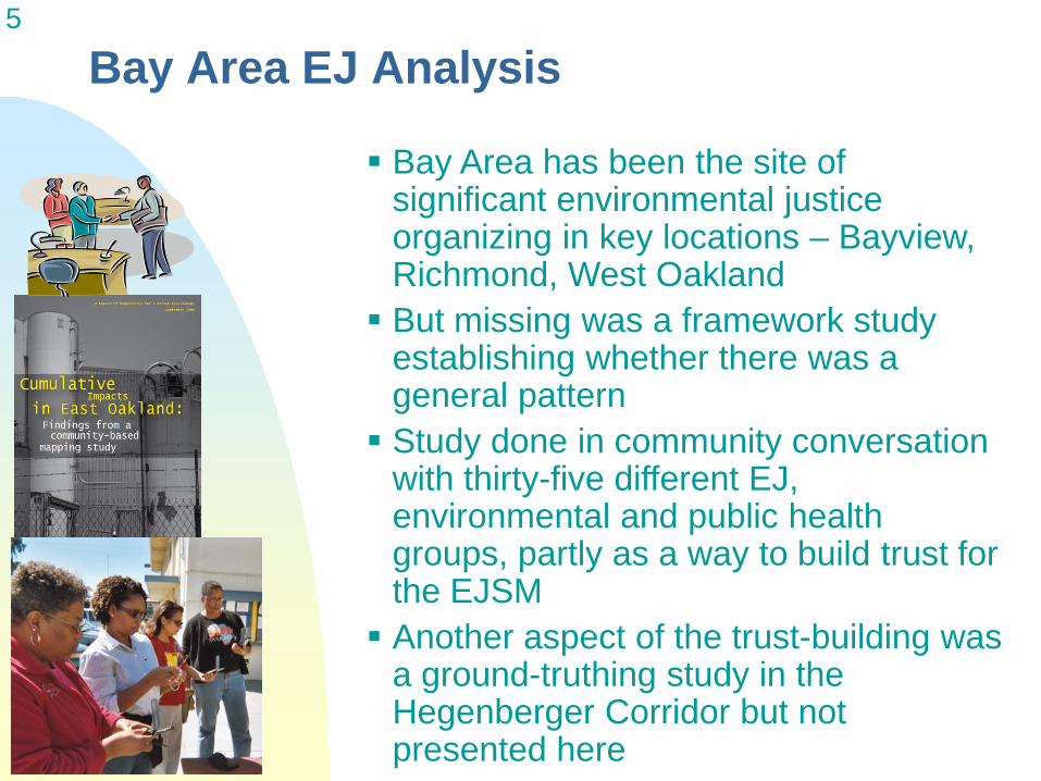
Bay Area EJ Analysis
Bay Area has been the site of significant environmental justice organizing in key locations – Bayview, Richmond, West Oakland But missing was a framework study
establishing whether there was a general pattern Study done in community conversation
with thirty-five different EJ,environmental and public health groups, partly as a way to build trust for the EJSM Another aspect of the trust-building was
a ground-truthing study in the Hegenberger Corridor but notpresented here
6
Assembling the Data for Analysis Toxic Release Inventory – annual self-reports
from point facilities, with analysis attempting to separate out carcinogenic releases, and facilities geocoded as of 2003. The TRI data is standard in national studies although much analysis is flawed due to poor geographic matching.
NATA – National Air Toxics Assessment (1999). Takes into account national emissions database with modeling of stationary, mobile, and point sources. Publicly available NATA fails to account for cancer risk associated with diesel; we apply risk factors to modeled diesel to complete the California picture.
###############SSSSSSSSSSSSSSSSSSSSSSSS #####SSSSS#S #S S#############SSSSSSSSSSSS ####SSS#################SSSSSSSSSSSSSSSSSS# #S S
######SSSSSS##SS######SSSSSS
##SS
#S###SSS
##SS#S
7 At First Glance . . . San Francisco Bay Area, 2003 Toxic Release Inventory Air Release FacilitiesTRI Facilities Relative to Neighborhood Demographicsby 2000 Census Tract Demographics
Toxic Release Inventory S# Air ReleaseFacilities (2003)
Percent People of Color < 34% 34 - 61% > 61%
0 10 20 Miles
#S
#S#S #S#S#S ## SS #S S#S ## #SS #S # SS #S## #SS #S# S #S #S S#S
#S #S
#S #S#S#S#S #S #S#S #S#S#S#S #S #S#S ##S
#S#S #S#S#S ## SS ## SS #S
#S #S#S # #S S#S# #S S #S#S##SS #S #S#S #S#S #S#SS ## S #S##S#S#S S# ## S SS# #S # SS #S#S#S
8How do we determine TRI proximity? The one-mile case
#
# 1-Mile Radius
280 # TRI Facility.,-Census Tract Boundaries
.,-380 Total Population by Census Block0 - 10 10 - 100 100 - 1000 N
# 1000 + 0.5 1 Miles 0
9
Population by Race/Ethnicity (2000) and Proximity to a TRI Facility with Air Releases (2003) in the 9-County Bay Area
100%
Perc
enta
ge o
f Pop
ulat
ion
80%
60%
40%
20%
0%
33% 45%
63%
30%
21%
12%12% 8%
4%
20% 21% 17%
4% 4% 4%
within 1 mile 1 to 2.5 miles more than 2.5 miles away
Proximity to an active TRI
Other
Asian/Pacific Islander
African American
Latino
Non-Hispanic White
■
□
□
■
□
Differences by Proximity:
10 TRI Facilities Relative to NeighborhoodDemographics Aside from Race
TRI Proximity
Between 1 More than Less than mile and 2.5 miles
Variables 1 mile 2.5 miles away
% persons in poverty 12% 9% 6%
Median per capita income $19,702 $25,140 $34,187 % home owner 52% 57% 61% % industrial, commercial and transportation land use 17% 9% 5% Population density (persons per square mile) 9,202 10,107 9,748 % manufacturing employment 19% 16% 12% % recent immigrants (1980s and later) 26% 21% 15%
% linguistically isolated households 12% 9% 6%
.......
■ ■ ■ ■ ■ ■ ---
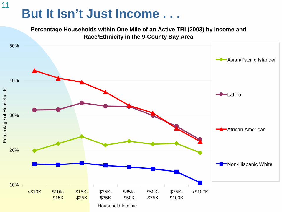
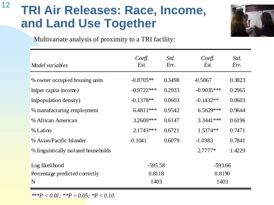
11 But It Isn’t Just Income . . .
Percentage Households within One Mile of an Active TRI (2003) by Income and Race/Ethnicity in the 9-County Bay Area
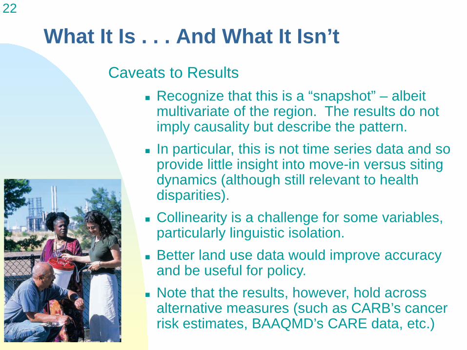
What It Is . . . And What It Isn’t Caveats to Results
Recognize that this is a “snapshot” – albeit multivariate of the region. The results do not imply causality but describe the pattern.
In particular, this is not time series data and so provide little insight into move-in versus siting dynamics (although still relevant to health disparities).
Collinearity is a challenge for some variables, particularly linguistic isolation.
Better land use data would improve accuracy and be useful for policy.
Note that the results, however, hold across alternative measures (such as CARB’s cancer risk estimates, BAAQMD’s CARE data, etc.)
$pat1JI AulOCOlftlMIOII fun<:111)n for fnt lmagt
23
Takeaways from This Analysis
Analytic: There is a pattern and it holds even we
control for spatial autocorrelation Important findings are linguistic isolation
which may have policy implications Process:
Engaging communities in research process strengthens research and policy relevance
It also builds trust in what can be complicated processes such as the eventual goal of this project: the EJSM.
24
Birth Outcomes and Air Pollution
25
Methods: data sources
California natality files 1996-2006 Information on live births & mothers
CalAIRS database CO & O3 daily maximum 8 hour average. NO2,SO2, PM10, & PM2.5 daily averages. PM estimated by subtracting PM2.5 from PM10coarse
US Census 2000 Poverty rate (proportion of residents living in households under
FPL) Unemployment rate (workers 16 and older seeking work) Home ownership rate (owner-occupied vs. renter-occupied) Low educational attainment (population over age 25 with less
than a high school education)
26
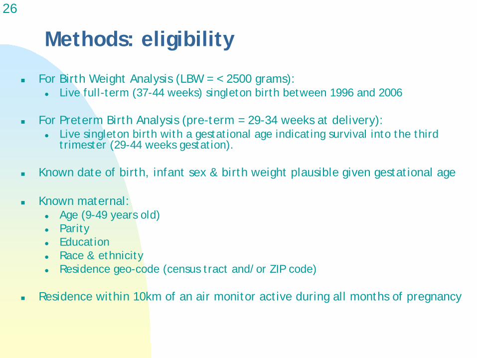
Methods: eligibility
For Birth Weight Analysis (LBW = < 2500 grams): Live full-term (37-44 weeks) singleton birth between 1996 and 2006
For Preterm Birth Analysis (pre-term = 29-34 weeks at delivery): Live singleton birth with a gestational age indicating survival into the third
trimester (29-44 weeks gestation).
Known date of birth, infant sex & birth weight plausible given gestational age
Known maternal: Age (9-49 years old) Parity Education Race & ethnicity Residence geo-code (census tract and/or ZIP code)
Residence within 10km of an air monitor active during all months of pregnancy
27
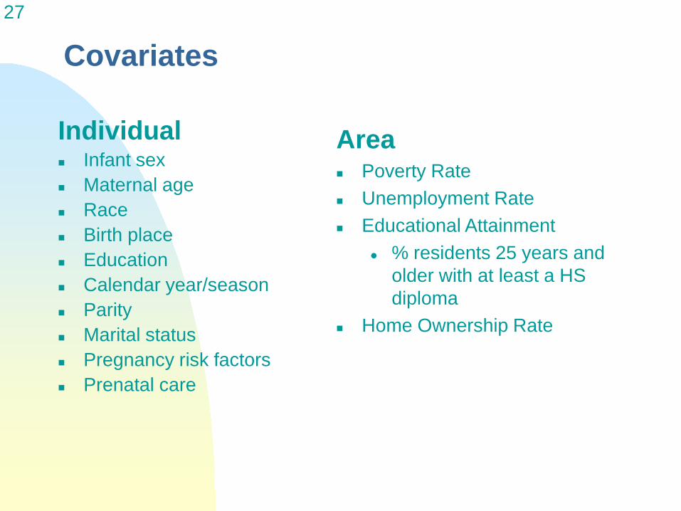
Covariates
Individual Infant sex Maternal age Race Birth place Education Calendar year/season Parity Marital status Pregnancy risk factors Prenatal care
Area Poverty Rate Unemployment Rate Educational Attainment
% residents 25 years and older with at least a HS diploma
Home Ownership Rate
28
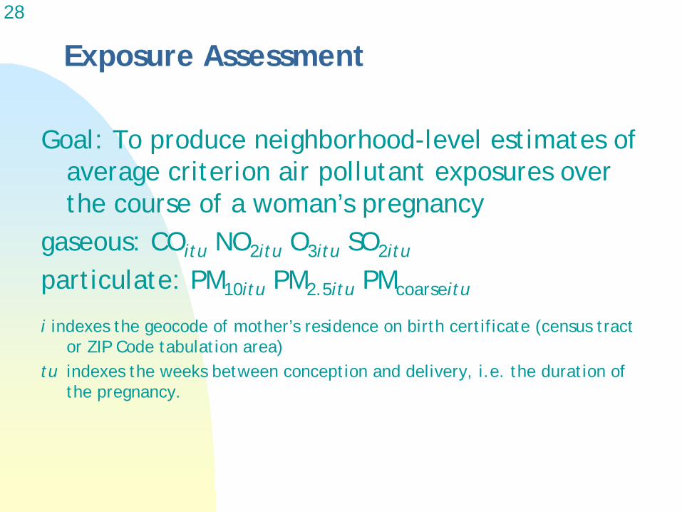
Exposure Assessment
Goal: To produce neighborhood-level estimates of average criterion air pollutant exposures over the course of a woman’s pregnancy
gaseous: COitu NO2itu O3itu SO2itu
particulate: PM10itu PM2.5itu PMcoarseitu
i indexes the geocode of mother’s residence on birth certificate (census tract or ZIP Code tabulation area)
tu indexes the weeks between conception and delivery, i.e. the duration of the pregnancy.
29
Overview
For each geo-reference, in each week, for each pollutant, calculate: 1) pollutant level from closest monitor* 2) distance to monitor
* We have calculated both nearest neighbor (the approach used in the analyses) and also an IDW averaged value, but since the monitoring network is sparse, these are interchangeable in most cases.
For each pregnancy, average the weekly pollutant levels across the duration of the pregnancy for the mother’s residential georeference, only for those measures within a specified distance (2km, 3km, 5km, 10km)
Use AQS & CalAIRS.
For each monitor in each week:
Calculate daily summary average of 18-24 hourly measures, fewer than 18 hourly measures discarded
Calculate weekly summary average of daily summaries only one daily summary required to assign a weekly summary
Specifics Verify monitor locations.
For each census block, find nearest monitor active during week, assign pollutant level from that monitor.
Aggregate blocks into: census tracts (2000) census tracts (1990) ZCTA’s (200)
For each pregnancy: Calculate monthly
summaries average of at least 3 weekly summary exposure measures, otherwise discarded
Calculate trimester-specific exposures 1st: average of first 4 monthly summaries 2nd: average months 5 to 7 3rd: average months 8 to 10 (less if pregnancy shorter)
Full pregnancy exposure average all months of pregnancy (if any one month invalid, then full pregnancy invalid)
31
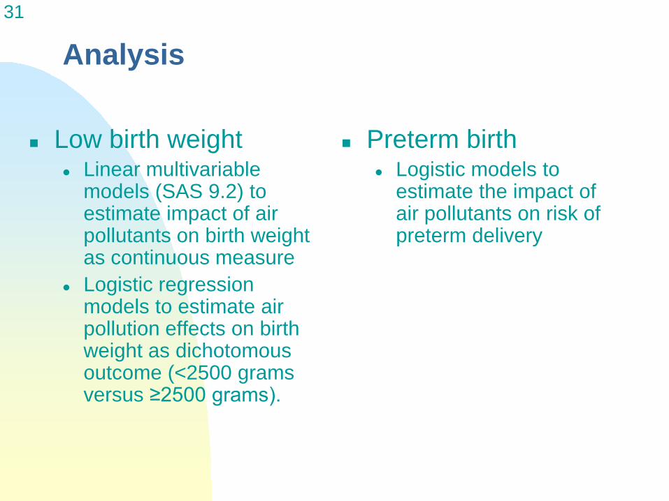
Analysis
Low birth weight Linear multivariable
models (SAS 9.2) to estimate impact of airpollutants on birth weight as continuous measure
Logistic regression models to estimate air pollution effects on birth weight as dichotomousoutcome (<2500 grams versus ≥2500 grams).
Preterm birth Logistic models to
estimate the impact of air pollutants on risk of preterm delivery
70%
60%
50%
40%
30%
20%
10%
0%
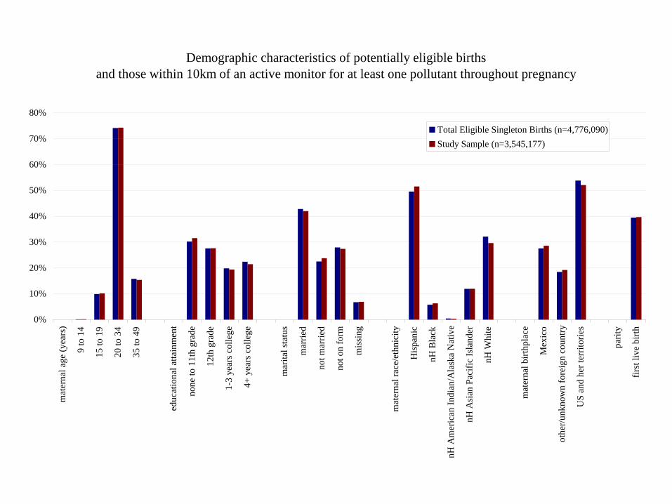
Demographic characteristics of potentially eligible births and those within 10km of an active monitor for at least one pollutant throughout pregnancy
80%
Total Eligible Singleton Births (n=4,776,090) Study Sample (n=3,545,177)
mat
erna
l age
(yea
rs)
9 to
14
15 to
19
20 to
34
35 to
49
educ
atio
nal a
ttain
men
t
none
to 1
1th
grad
e
12th
gra
de
1-3
year
s col
lege
4+ y
ears
col
lege
mar
ital s
tatu
s
mar
ried
not m
arrie
d
not o
n fo
rm
mis
sing
mat
erna
l rac
e/et
hnic
ity
His
pani
c
nH B
lack
nH A
mer
ican
Indi
an/A
lask
a N
ativ
e
nH A
sian
Pac
ific
Isla
nder
nH W
hite
mat
erna
l birt
hpla
ce
Mex
ico
othe
r/unk
now
n fo
reig
n co
untry
US
and
her t
errit
orie
s
parit
y
first
live
birt
h
33
Results
Pre-term birth (3.1%)
A ◊ ◊ A
?
A A ◊
◊
◊ A
A
A
A
A A
◊ ◊ ? A
A
Odd
Rat
io
1.3
1.2
1.1
CO,
per
ppm
at 3
km
at 5
km
at 1
0km
NO
2, p
er p
phm
at 3
km
at 5
km
at 1
0km
O3,
per
pph
m
at 3
km
at 5
km
at 1
0km
SO2,
per
ppb
at 3
km
at 5
km
at 1
0km
odds ratio of premature delivery (29-34 vs. 39-44 weeks), per change in full-pregnancy gaseous air pollutant average exposure
odds ratio of premature delivery (29-34 vs. 39-44 weeks), per change in full-pregnancy gaseous air pollutant average exposure, models controlled
for maternal & neighbohood characteristics, 3km, 5km, 10km CO
, pe
r pp
m
at 3
km
at 5
km
at 1
0km
NO
2, p
er p
phm
at 3
km
at 5
km
at 1
0km
O3,
per
pph
m
at 3
km
at 5
km
at 1
0km
SO2,
per
ppb
at 3
km
at 5
km
at 1
0km
1.00
0.90
A A
A
◊ ◊
◊ A A
A
A
◊ A
◊ ◊
A A
A A ◊ ◊
◊ A
A
1.3
1.2
1.1 Odd
s Ra
tio
odds ratio of premature delivery (29-34 vs. 39-44 weeks), per change in full-pregnancy particulate matter average exposure,
crude models, 3km, 5km, 10km PM
10,
per
10μg/m
3
at 3
km
at 5
km
at 1
0km
PM2.
5, p
er
10μg/m
3
at 3
km
at 5
km
at 1
0km
PMco
arse
, pe
r 10
μg/m
3
at 3
km
at 5
km
at 1
0km
1
0.9
A A
A
◊ ◊ A
A ◊ ◊
◊ A
A ◊ A A
A A
◊ ◊ A
A
1.30
1.20
1.10 Odd
s Ra
tio
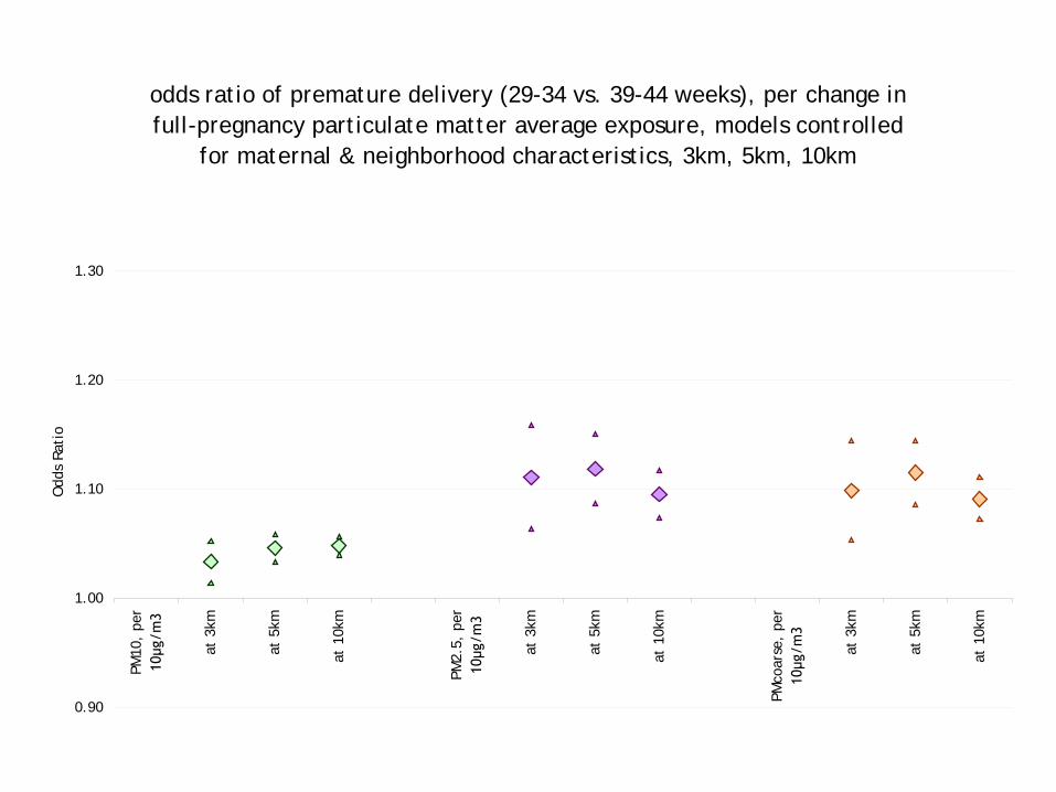
odds ratio of premature delivery (29-34 vs. 39-44 weeks), per change in full-pregnancy particulate matter average exposure, models controlled
for maternal & neighborhood characteristics, 3km, 5km, 10km PM
10,
per
10μg/m
3
at 3
km
at 5
km
at 1
0km
PM2.
5, p
er
10μg/m
3
at 3
km
at 5
km
at 1
0km
PMco
arse
, pe
r 10
μg/m
3
at 3
km
at 5
km
at 1
0km
1.00
0.90
t t t t + + + ❖
+ + t t _______!__t - -
1.2
odds
ratio
of p
rete
rm b
irth
per c
hang
e in
pol
luta
nt le
vel t
hrou
ghou
t pre
gnan
cy
1.1
1.0
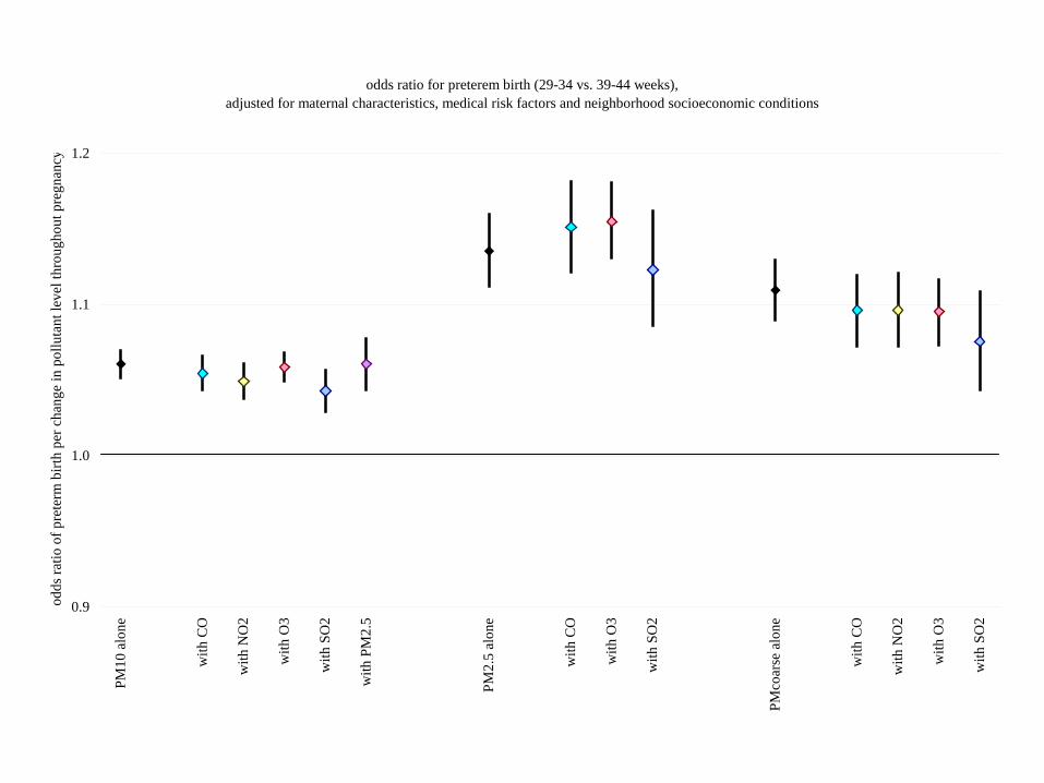
odds ratio for preterem birth (29-34 vs. 39-44 weeks), adjusted for maternal characteristics, medical risk factors and neighborhood socioeconomic conditions
CO
alo
ne
with
O3
with
PM
10
NO
2 al
one
with
O3
with
PM
10
O3
alon
e
with
CO
with
NO
2
with
PM
10
PM10
alo
ne
with
CO
with
NO
2
with
O3
0.9
t t t t t t
1.2
odds
ratio
of p
rete
rm b
irth
per c
hang
e in
pol
luta
nt le
vel t
hrou
ghou
t pre
gnan
cy
1.1
1.0
odds ratio for preterem birth (29-34 vs. 39-44 weeks), adjusted for maternal characteristics, medical risk factors and neighborhood socioeconomic conditions
PM10
alo
ne
with
CO
with
NO
2
with
O3
with
SO
2
with
PM
2.5
PM2.
5 al
one
with
CO
with
O3
with
SO
2
PMco
arse
alo
ne
with
CO
with
NO
2
with
O3
with
SO
2
0.9
42
Results
Low Birth Weight (2.3%)
t
5
gram
s birt
h w
eigh
t per
cha
nge
in p
ollu
tant
leve
l
0
-5
-10
-15
-20
Difference in birth weight associated with full pregnancy gaseous pollutant exposures for births within 10 km monitor distance, single and two-pollutant
CO
alo
ne
with
O3
with
SO
2
with
PM
10
with
PM
2.5
with
PM
coar
se
NO
2 al
one
with
O3
with
SO
2
with
PM
10
with
PM
2.5
with
PM
coar
se
O3
alon
e
with
CO
with
NO
2
with
SO
2
with
PM
10
with
PM
2.5
with
PM
coar
se
linear models
t t t gram
s birt
h w
eigh
t per
cha
nge
in p
ollu
tant
leve
l
-5
-10
-15
-20
0
5
PM10
alo
ne
with
CO
with
NO
2
with
O3
with
SO
2
with
PM
2.5
PM2.
5 al
one
with
CO
with
O3
with
SO
2
PMco
arse
alo
ne
with
CO
with
NO
2
with
O3
with
SO
2
Difference in birth weight associated with full pregnancy particulate pollutant exposures for births within 10 km monitor distance, single and two-pollutant
linear models
♦ ♦
+ + ♦
t gram
s birt
h w
eigh
t per
cha
nge
in p
ollu
tant
leve
l .
per p
pm C
O
His
pani
cs
non-
His
pani
c B
lack
s
non-
His
pani
c A
sian
s & P
acifi
c Is
land
ers
non-
His
pani
c W
hite
s
per p
phm
NO
2
His
pani
cs
non-
His
pani
c B
lack
s
non-
His
pani
c A
sian
s & P
acifi
c Is
land
ers
non-
His
pani
c W
hite
s
per p
phm
ozo
ne
His
pani
cs
non-
His
pani
c B
lack
s
non-
His
pani
c A
sian
s & P
acifi
c Is
land
ers
non-
His
pani
c W
hite
s
Difference in birth weight in grams associated with full pregnancy gaseous pollutant exposures for births within 10 km monitor distance,
stratified by maternal race and ethnicity
-30
-20
-10
0
10
♦ f t ♦ + t t
+ t
gram
s birt
h w
eigh
t per
cha
nge
in p
ollu
tant
leve
l .
per 1
0μg/
m3
of P
M10
His
pani
cs
non-
His
pani
c B
lack
s
non-
His
pani
c A
sian
s & P
acifi
c Is
land
ers
non-
His
pani
c W
hite
s
per 1
0μg/
m3
of P
M2.
5
His
pani
cs
non-
His
pani
c B
lack
s
non-
His
pani
c A
sian
s & P
acifi
c Is
land
ers
non-
His
pani
c W
hite
s
per 1
0μg/
m3
of P
Mco
arse
His
pani
cs
non-
His
pani
c B
lack
s
non-
His
pani
c A
sian
s & P
acifi
c Is
land
ers
non-
His
pani
c W
hite
s
-30
-20
-10
0
10
Difference in birth weight in grams associated with full pregnancy particulate pollutant exposures for births, stratified by maternal race
and ethnicity
47
Summary of findings
Modest relationship between ambient criteria air pollutant exposure (PM2.5, PM10, coarse PM, CO, NO2 and O3) and lower average birth weight among full-term infants as well as higher risk of preterm birth.
Associations between increasing pollutant exposures and decrements in birth weight and risk of preterm delivery persist during different trimesters
Strongest effects seen for exposures during the entire gestational period.
Did not find consistent evidence of effect modification PM2.5 and course PM effect estimates strongest for African
Americans
48
Caveats
Smoking: Has a large effect on birth weight, but in studies of
ambient air pollution not a significant confounder Limits of single pollutant analysis:
Future work can take source-based approach to assessing health effects rather than isolating the impacts of individual pollutants (e.g traffic density)
Does not account for transient spikes in air pollutant levels (e.g. fires)
49 Implications
Small difference in means
Large difference in area under
the curve
^Clinically relevant level
Small shift in the population distribution of birth weights may have broader health implications that need to be further examined.
50 Purpose of Environmental JusticeScreening Methodology (EJSM)
Develop indicators of cumulative impact that: Reflect research on air pollution, environmental
justice, and health Are transparent and relevant to policy-makers and
communities Reviewed by community EJ groups, California Air
Resources Board, academic peers and other agencies
Apply EJ “screening method” to multiple uses: Local land use planning
(e.g. Los Angeles, City of Commerce & Richmond – community plans)
Regulatory decision-making and enforcement Community outreach
51 Focus of EJSM
Developed with specific reference to ambient air quality in neighborhoods
Not screening for occupational, indoor, water or pesticides.
Developed to incorporate land use information into environmental decision-making
Performs best with detailed and high spatial resolution land use data.
Developed using publically available secondary databases, not micro-studies
This is screening not assessment
y zar la
al e o
OC al 111 y
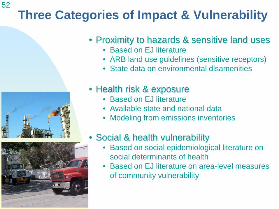
52 Three Categories of Impact & Vulnerability
• Proximity to hazards & sensitive land uses • Based on EJ literature • ARB land use guidelines (sensitive receptors) • State data on environmental disamenities
• Health risk & exposure
• Social & health vulnerability
4/20/2010
• Based on EJ literature • Available state and national data • Modeling from emissions inventories
• Based on social epidemiological literature on social determinants of health
• Based on EJ literature on area-level measures of community vulnerability
,..____ EJSM Completed
In Progress
D Air Basins
53
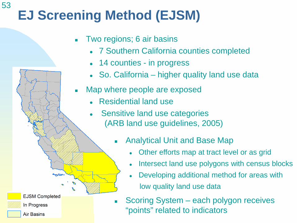
14 counties - in progress
Map where people are exposed Residential land use
EJ Screening Method (EJSM) Two regions; 6 air basins
7 Southern California counties completed
So. California – higher quality land use data
Sensitive land use categories (ARB land use guidelines, 2005)
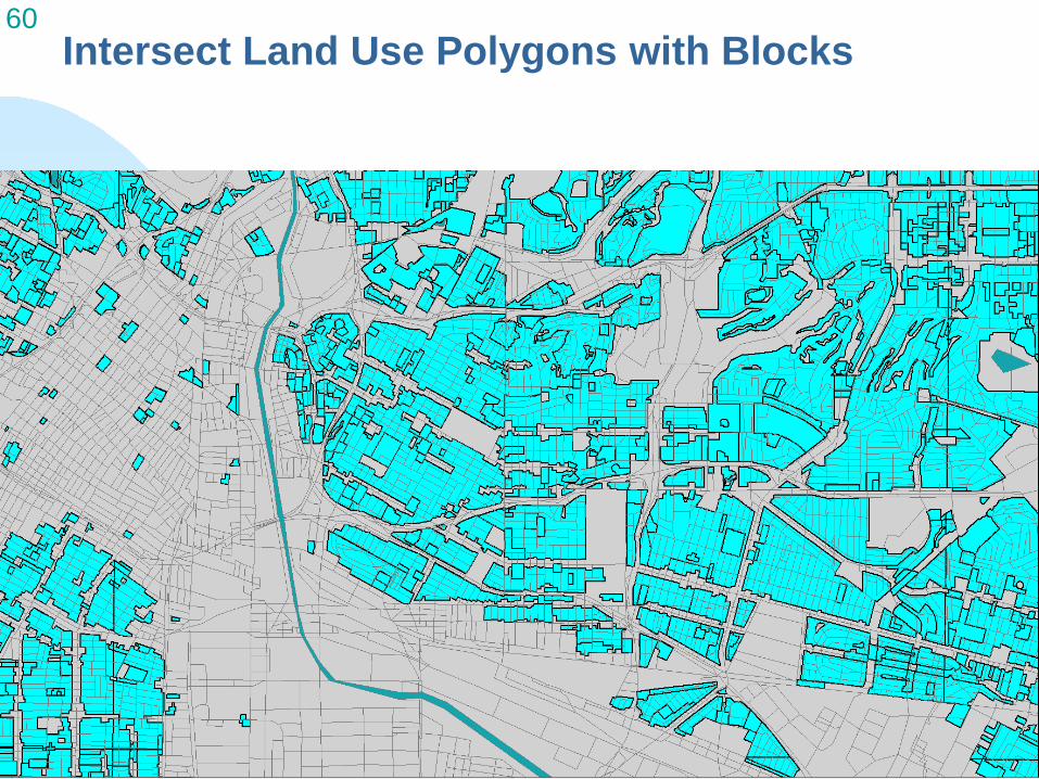
Analytical Unit and Base Map Other efforts map at tract level or as grid Intersect land use polygons with census blocks Developing additional method for areas with
low quality land use data
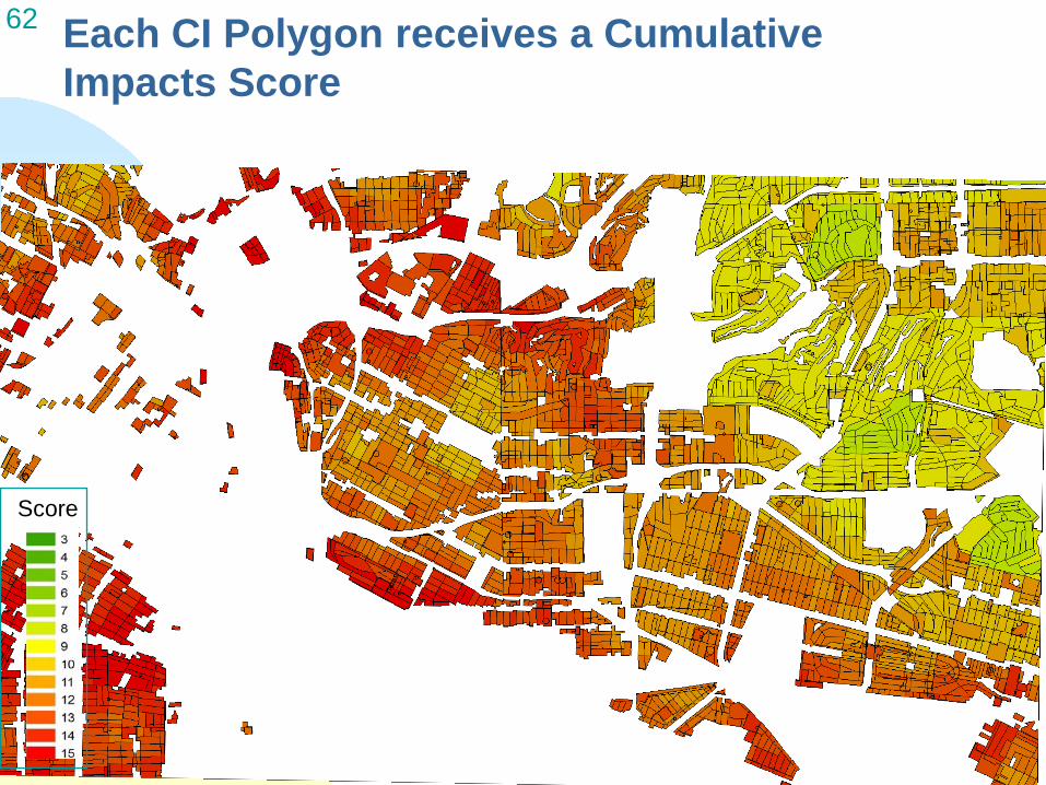
Scoring System – each polygon receives “points” related to indicators
54 Screening Method Architecture
Metrics & CI Scoring
QA/QC
Linking & Mapping
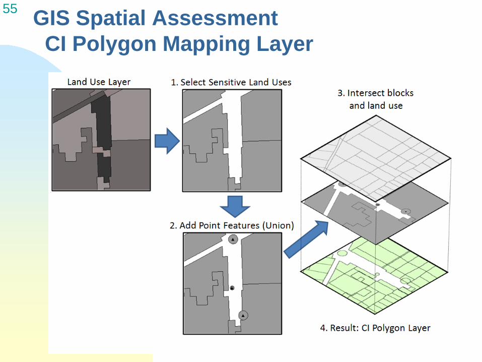
Step 1: GIS Spatial Assessment Derive land use layer – select land use types Create CI polygon mapping layer (intersect land use
polygons with census blocks) Calculate land use and hazard proximity metrics for
CI polygons
Step 2: Programming (SPSS) Data processing and cleaning Metrics development and ranking Derivation of CI scores
By category (Risk, hazard proximity, SES) Total CI score
Analytics This work can be done in SAS or R
Step 3: GIS Mapping of Results
Essential to Steps 1 and 2: Quality control of data layers Document and verify metric derivation and scoring
Use Layer 1. Select Sensit ive Land Uses
,..J
2. Add Point Features (Union)
0
3. Int ersect blocks
and land use
4. Resu lt : Cl Polygon Layer
55 GIS Spatial Assessment CI Polygon Mapping Layer
a dU e oc c ee
(
\
• go ere eo
~
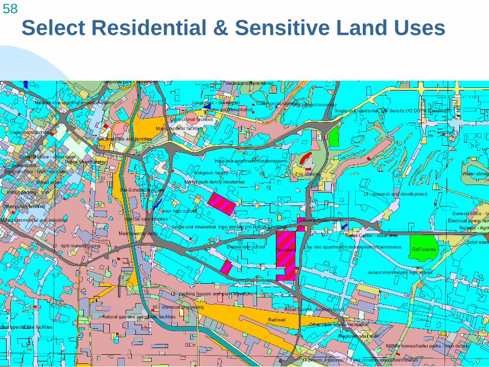
56 Land Use – Focus screening on where people live Dark Gray = Industrial, Transportation, etc.; Light Gray = Open Space, Vacant, etc. White = Residential and Sensitive Land Uses – only these areas are scored
57 Southern California Assoc. of Governments (SCAG) 2005 Land Use Polygons
Cemetery—No one ‘living’ here
58
Select Residential & Sensitive Land Uses
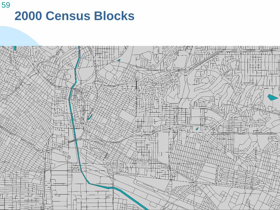
59 2000 Census Blocks
60
Intersect Land Use Polygons with Blocks
1,f;&?
\) ~ ~
~~ 0 □ Po 6) <'.l: <l
"0 v><t, !Ji Ll
ca
Q
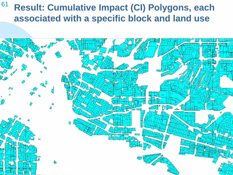
61 Result: Cumulative Impact (CI) Polygons, each associated with a specific block and land use
~; • ~~ #
◊ ' I • .,
- 3 -4 -5 6
7
8 -9
10 11
- 12 - • - 13 ' - 14 - 15
62 Each CI Polygon receives a Cumulative Impacts Score
Score
63 Sensitive Land Uses
Defined by ARB Air Quality and Land Use Handbook, 2005
Identified from different data sources SCAG 2005 land use data layer (GIS polygons) Automated from address lists (geocoded points)
Childcare facilities (SCAG, NAICS address list)
Healthcare facilities (CaSIL/SCAG)
Schools (SCAG, CA Dept of Education)
Urban Playgrounds & Parks (SCAG)
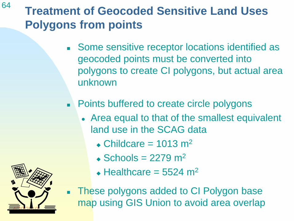
64 Treatment of Geocoded Sensitive Land Uses Polygons from points
4/20/2010
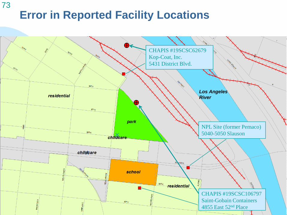
Some sensitive receptor locations identified as geocoded points must be converted into polygons to create CI polygons, but actual area unknown
Points buffered to create circle polygons Area equal to that of the smallest equivalent
land use in the SCAG data Childcare = 1013 m2
Schools = 2279 m2
Healthcare = 5524 m2
These polygons added to CI Polygon base map using GIS Union to avoid area overlap
60TH
school
AllEY
~~======16~-~~~~ ~-------
res id . ntial school
rsidential
65 Geocoded Sensitive Land Uses - Polygons from points (City of Maywood)
Maywood Preschool Academy (point)
St. Rose of Lima Parish School (polygon) Maywood Pre-K Education
Center (point)
SCAG Land Use Polygon “under construction” Emmanuel Health Care
Center (point)
SouthEast Area New Learning Center LAUSD (point)
Nueva Vista Elementary LAUSD (polygon)
66 Geocoded Sensitive Receptor Land Uses Polygons from points
Maywood Preschool
St. Rose of Lima Parish School (polygon)
Academy (point)
Emmanuel Health Care Center (point)
Maywood Pre-K Education Center (point)
SouthEast Area New Learning
SCAG Land Use Polygon “under construction”
Center LAUSD (point)
Nueva Vista Elementary LAUSD (polygon)
d Uses No Sensitive Lan d
Contains Sensitive Lan
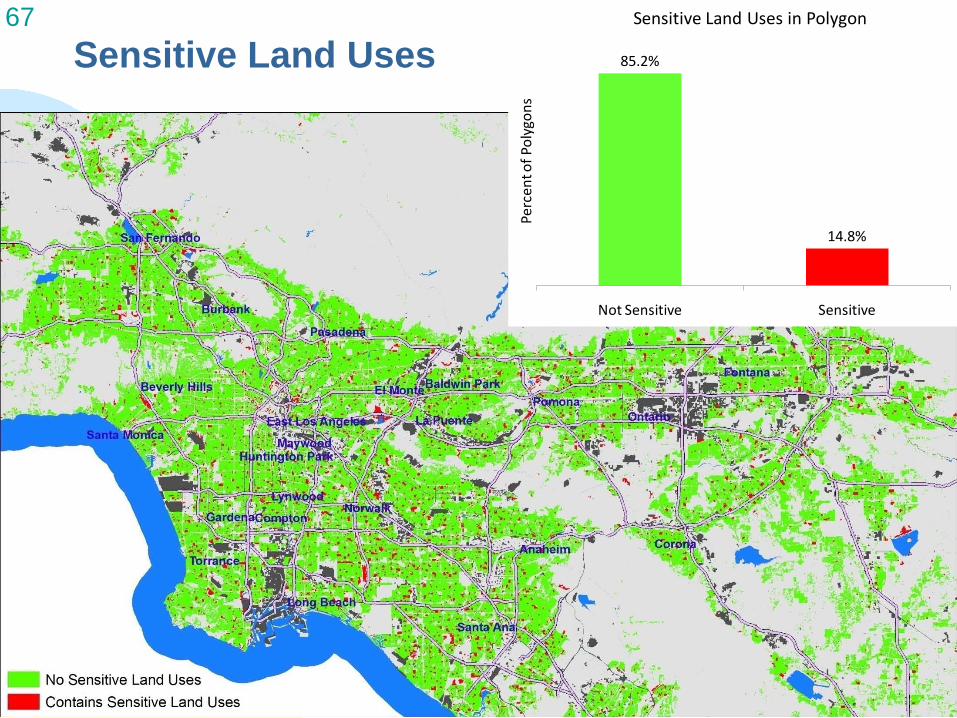
67 Sensitive Land Uses in Polygon
85.2% Sensitive Land Uses
14.8%
Not Sensitive Sensitive
Perc
ent o
f Pol
ygon
s
68 GIS Spatial Assessment
Calculate hazard proximity and sensitive land use metrics
Initial analysis using CI polygons
Transferred to census tracts using a population-weighting procedure
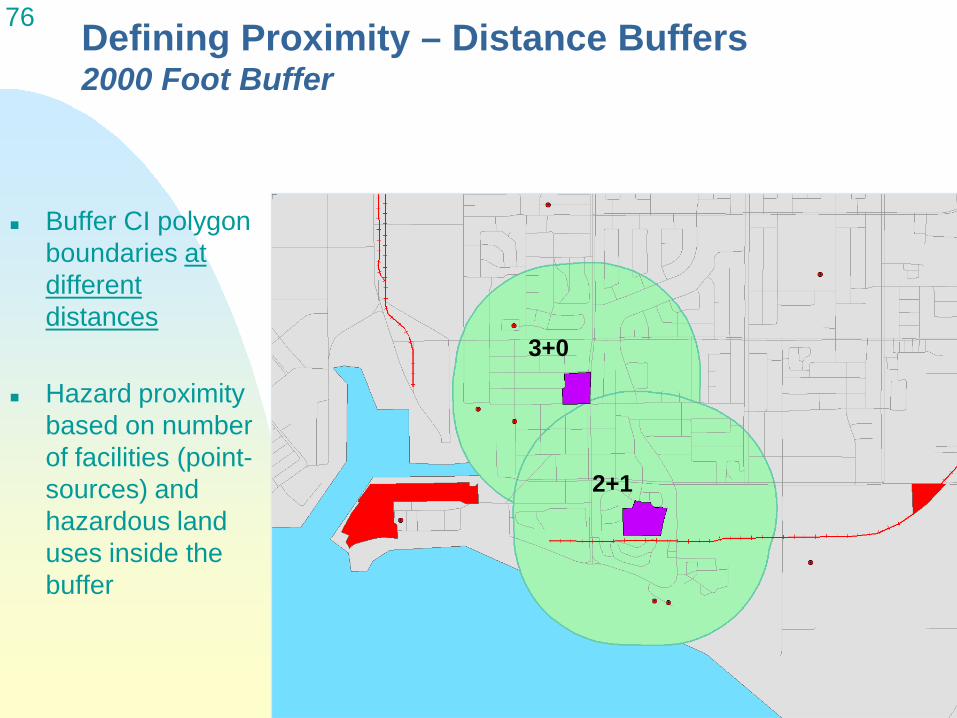
69 Proximity to Air Pollution Sources & Hazardous Land Uses
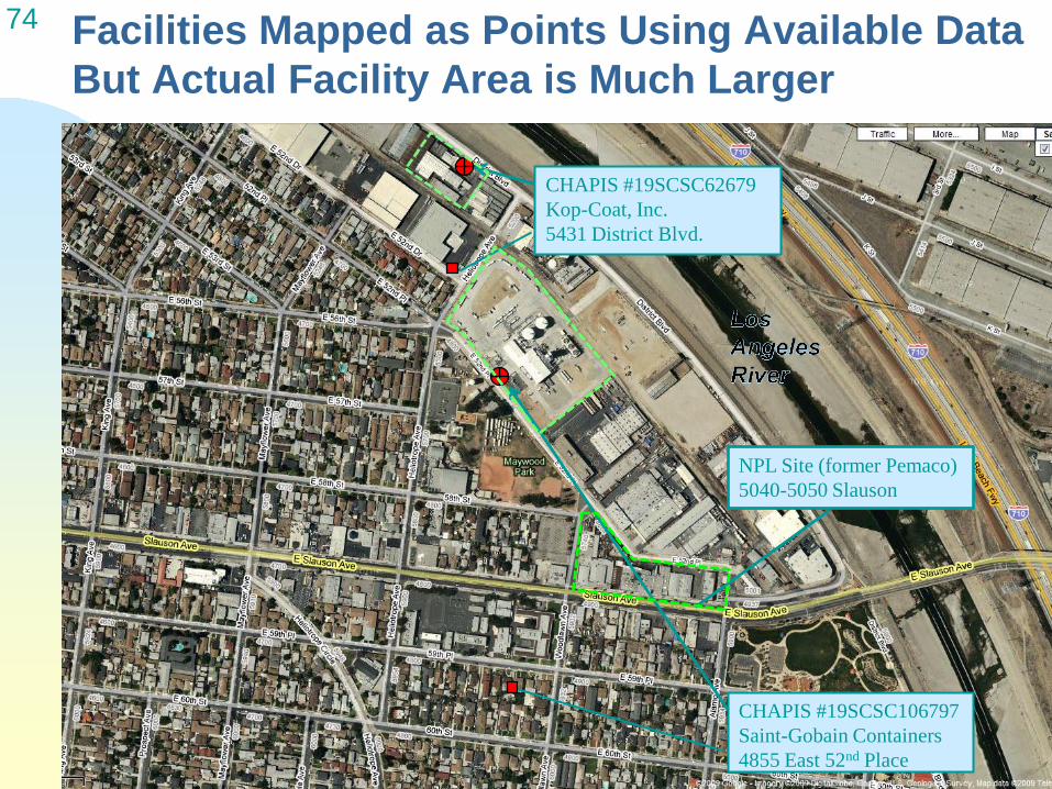
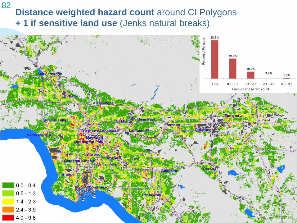
82 Distance weighted hazard count around CI Polygons + 1 if sensitive land use (Jenks natural breaks)
55.8%
29.3%
10.2% 3.8% 1.0%
Perc
ent o
f Pol
ygon
s
< 0.5 0.5 - 1.3 1.4 - 2.3 2.4 - 3.9 4.0 - 9.8 Land use and hazard count
83 Calculating Hazard Proximity & Sensitive Land Counts at the Tract Level Why? Tracts are a consistent level of geography for many
sources of data; avoid misrepresenting precision
All of the health risk and social vulnerability measures (discussed later) are available at the tract level
How Calculated:
Estimate population in each CI polygon (area-weighting of population of its host block)
Calculate population-weighted average of the hazard and sensitive land use counts across the CI Polygons within each census tract
D No data
1111 0.0- 0.5
0.5 - 1.2
1.2-2.3
1111 2.3-4.0 1111 4.0- 8.0
84 Tract-level Hazard Proximity & Sensitive Land Use Counts Distance weighted hazard count (+1 if sensitive land use), population weighted to the tract level (Jenks natural breaks)
85 Tract-level Hazard Proximity & Sensitive Land Use Counts Distance weighted hazard count (+1 if sensitive land use), population weighted to the tract level, mapped on CI Polygons (Jenks natural breaks)
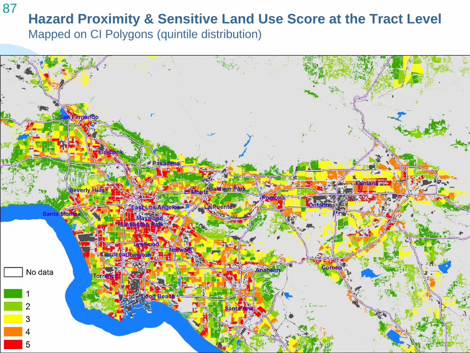
86 Hazard Proximity & Sensitive Land Use Scores at the Tract Level Tract-level hazard and sensitive land use counts are
ranked into quintiles across all tracts in the region
Assigned score of 1-5 based on quintile rank - final hazard proximity and sensitive land use score at the tract level
Quintile distribution is used throughout the EJ Screening Method because it is an accessible and recognizable ranking procedure
• No “right” distribution to follow (magnitudes of hazards unknown)
87 Hazard Proximity & Sensitive Land Use Score at the Tract Level Mapped on CI Polygons (quintile distribution)
88 Health Risk & Exposure Indicators (Tract Level)
RSEI (Risk Screening Environmental Indicators) (2005) toxic conc. hazard scores from TRI facilities
NATA 1999 (National Air Toxics Assessment) Respiratory hazard from mobile & stationary sources
CARB Estimated Inhalation Cancer Risk 2001 Calculated from modeled air toxics concentrations using emissions from CHAPIS (mobile & stationary) Corrected version of this data
CARB estimated PM2.5 concentration
CARB estimated Ozone concentration
89 Health Risk & Exposure Scores (Tract Level)
Each health risk indicator is ranked into quintiles (1-5) across all tracts in the region
Quintile rank values are summed by tract across all indicators
These tract sums are ranked once again into quintiles and assigned scores 1-5.
The resulting quintile rank for each tract is it’s final health risk score
90 Health Risk & Exposure Score at the Tract Level Mapped on CI Polygons (quintile distribution)
91 Social & Health Vulnerability Indicators Census Tract Level Metrics (2000)
% residents of color (non-White)
% residents below twice national poverty level
Home ownership - % living in rented households
Housing value – median housing value
Educational attainment – % population > age 24 with less than high school education
Age of residents (% <5)
Age of residents (% >60)
Linguistic isolation - % pop. >age 4 in households where no one >age 15 speaks English well
Voter turnout - % votes cast among all registered voters in 2000 general election
Birth outcomes – % preterm or SGA infants 1996-03
92 Social & Health Vulnerability Scores Each social and health vulnerability metric is ranked into quintiles (1-5) across all tracts in the region
Final score is derived by taking average ranking (across all metrics) for each tract, and ranking the average once again into quintiles (1-5)
A note on missing values: To help ensure that the social and health vulnerability scores are reliable, we exclude tracts with less than 50 people, and those with 5 or more missing values among the 10 metrics considered. To account for missing values in tracts with 1 to 4 missing metrics, the average quintile ranking is taken across only the non-missing metrics.
,.J • • _J
D No data
1111 1 1111 2
3
1111 4 1111 s
. " r , ,. '-- "Q -
I ' , 'l_..- -·--~ .
_...,. -V ~ ... . .,,
I
-~
7·-i3?iJ~-.-. -~ ~ ""'" -,,.,,. -· I -
~ ! ~ ~~idf __ i -. - ~
. "''<:" "'' ·
.~ '\, --...."':'.,
' .. __,.
J
93 Social Health & Vulnerability Score at the Tract Level Mapped on CI Polygons (quintile distribution)
94
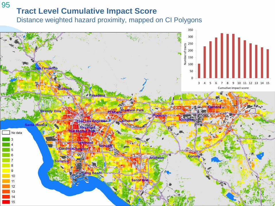
Cumulative Impact Scores at the Tract Level
Combine three categories of tract level impact and vulnerability to get Cumulative Impact Score
Cumulative Impact Score =
Hazard Proximity and Sensitive Land Use Score (1-5) +
Health Risk and Exposure Score (1-5) +
Social and Health Vulnerability Score (1-5)
Final Cumulative Impact Score Ranges from 3-15
. ·' ... -+<!IC,; ,!'• ,._ v. -~ ~ - .:. -rr~ ~ y ,~
"' ~ ~ ...... .... ~ .... . . .
~ I ~ J
. :;,...., ,· . ·. ~~ I • •
-3 -4 -5 -6 7
8
9
10
11
- 12
- 13
- 14
- 15
r ,I
.,, ♦ At-• -••
"'.
. .. r_ ' ,.,...,,. 0 ••11 -
,.... .· .
95 Tract Level Cumulative Impact Score Distance weighted hazard proximity, mapped on CI Polygons
98 Alternative Approach: Cumulative Impact Scores at the CI Polygon Level
Tract level health risk and exposure & social and health vulnerability scores (from above) are applied directly to the CI Polygons in each tract, but...
Hazard proximity and sensitive land use score is based on Jenks Natural Breaks with 5 categories rather than quintiles
Cumulative Impact Score =
Hazard Proximity and Sensitive Land Use Score (1-5) +
Health Risk and Exposure Score (1-5) +
Social and Health Vulnerability Score (1-5)
Final Cumulative Impact Score Ranges from 3-15
99
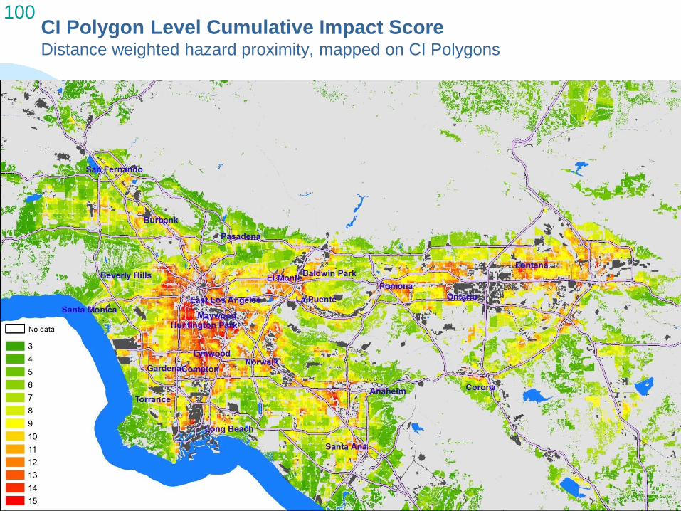
Cumulative Impact Scores at the CI Polygon Level
Why the CI Polygon Level?
Benefit:
Finer level of geography that preserves the accuracy of the hazard proximity & sensitive land use information – may be good for land-use decision making
Caution:
May give a false sense of geographic accuracy in the health risk & exposure and social & health vulnerability measure, which are derived at the tract level
Generally results in lower Cumulative Impact scores for CI Polygons that are not in upper reaches of the distribution of the hazard proximity & sensitive land use counts
100 CI Polygon Level Cumulative Impact Score Distance weighted hazard proximity, mapped on CI Polygons
101 Recommended Approach:
Tract Level Cumulative Impact Score using Distance Weighted hazard proximity is best…
The tract level is a appropriate geographic unit without overemphasizing precision of underlying data
Air quality and social demographic measures are available at the tract level
Using distance weighting on the hazard count: allows for flexibility in changing weights in
the face of new standards accounts better for geographic inaccuracies,
including the representation of some hazards as points with no geographic dimensions
102
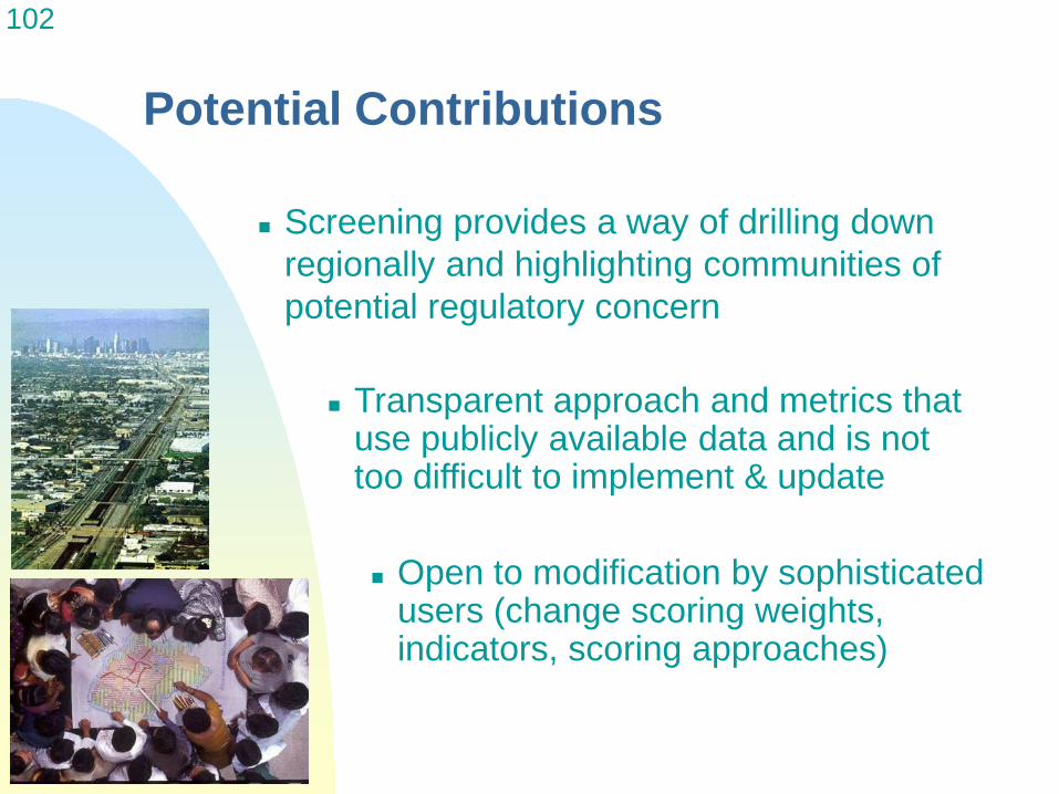
Potential Contributions
Screening provides a way of drilling down regionally and highlighting communities of potential regulatory concern
Transparent approach and metrics that use publicly available data and is not too difficult to implement & update
Open to modification by sophisticated users (change scoring weights,indicators, scoring approaches)
103
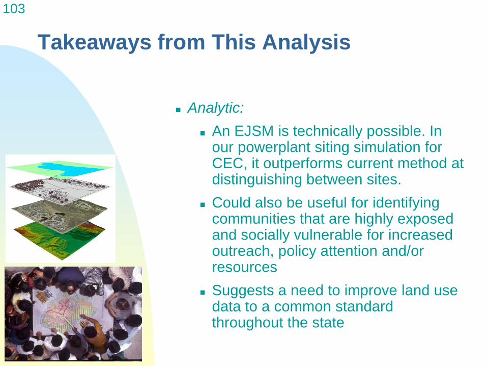
Takeaways from This Analysis
Analytic: An EJSM is technically possible. In
our powerplant siting simulation for CEC, it outperforms current method at distinguishing between sites.
Could also be useful for identifying communities that are highly exposed and socially vulnerable for increased outreach, policy attention and/or resources
Suggests a need to improve land use data to a common standard throughout the state
104
Takeaways from This Analysis
Process: Engaging communities in the
development of the method involvesrisks – will the information get out too early?
Community engagement also means making variable and ranking choices in ways that are intuitive and easier to explain
Such a process also builds trust in the potential use of the EJSM for policy and other purposes.