S C I E N C E O F T H E T O T A L E N V I R O N M E N T 3 9 6 ( 2 0 0 8 ) 1 8 0 – 1 9 2
ava i l ab l e a t www.sc i enced i rec t . com
www.e l sev i e r. com/ loca te / sc i to tenv
Integrating monitoring networks to obtain estimates ofground-level ozone concentrations — A proof ofconcept in Tuscany (central Italy)☆
Marco Ferrettia,⁎, Sara Andreia, Gabriella Caldinib, Daniele Grechib, Cristina Mazzalia,Emilio Galantic, Marco Pellegrinid
aLinnaeambiente Ricerca Applicata Srl, Via G. Sirtori 37, I-50137 Firenze, ItalybARPAT-Dipartimento di Firenze, Via Ponte alle Mosse 211, I-50144 Firenze, ItalycProvincia di Firenze, Dipartimento Sviluppo Territorio-Direzione Ambiente e Gestione Rifiuti, Via Mercadante 42, I-50144 Firenze, ItalydARPAT-Dipartimento di Lucca, Via Vallisneri 6 I-55100 Lucca (formerly at the Provincia di Firenze, Dipartimento Ambiente), Italy
A R T I C L E I N F O
☆ Project supported by the Provincia diresponsibility of the reported data and any s⁎ Corresponding author. Current address: Te
Article history:Received 13 November 2007Received in revised form1 February 2008Accepted 5 February 2008Available online 2 April 2008
Prior to 2000 anetwork of conventional ozone (O3) analysers existed in the Province of Firenze(Tuscany, central Italy). Between 2000 and 2004 the network was extended to incorporate anewly designed bioindicator network of tobacco plants (Nicotiana tabacum Bel W3). Theobjective was to set-up an integratedmonitoring system to obtain estimates of ground-levelO3 concentrations over the whole study area (3513 km2) in order to fill data gaps and coverreporting requirements. The existing conventional monitors were purposefully locatedmainly in urban areas. A total of 45 biomonitoring sites were selected using a systematicdesign to cover the target area. Two to five additional biomonitoring sites were co-locatedwith conventional O3 analysers for calibration purposes, and fivemore sites for independentvalidation ofmodelled O3 concentrations. Visible Leaf Injury Index (LII) on the tobacco plantswas significantly correlated (P: 0.018÷0.0014) with a series of O3 exposure variables (mean ofweekly 1-hour maxima, M1; mean of 7-hour means, M7; 24-hour mean, M24; and weeklyAOT40). LII was found to be a significant predictor of weekly means of the O3 exposurevariables with a standard error of estimates between 13.6 and 24.3 μg m−3 (absolute values).LII wasmappedwith an ad-hoc spatialmodel over the study area at a 2 ⁎2 kmgrid resolution,and mapped values were used to predict O3 concentrations by means of a first order linearmodel. Results showed that high estimates of O3 (up to 188 μg m−3 as mean of weeklymaxima, M1) occurred more frequently in hilly and mountainous areas, with a spatialpattern changing on an annual basis. Predicted O3 concentrations were not significantlydifferent from the measured concentrations (P: 0.34), although marked differences wereobserved for individual sites and years. The study provided evidence that integration ofmonitoring networks using differentmethods can be a viable option to obtain estimates of O3
Firenze, Dipartimento Sviluppo Territorio-Direzione Ambiente e Gestione Rifiuti. Theubsequent interpretation lies with the authors.rraData environmetrics, Dipartimento di Scienze Ambientali, Università di Siena, Via P.A.5415; fax: +39 0577 232896.rretti).
181S C I E N C E O F T H E T O T A L E N V I R O N M E N T 3 9 6 ( 2 0 0 8 ) 1 8 0 – 1 9 2
1. Introduction
Tropospheric ozone (O3) concentrations are considered to be ofserious environmental concern in Southern Europe and else-where (EEA, 2005). This is because: firstly, O3 concentrationshave increased steadily over the last century (Volz and Kley,1988) and are predicted to increase even further over thecoming decades, (e.g. Fowler et al., 1999; Vingarzan, 2004).Secondly, high O3 concentrations have been attributed toadverse effects on both human health (Brunekreef andHolgate, 2002) and vegetation (UN/ECE, 2004). Thirdly, tropo-spheric O3 has been recognised as significantly contributing toglobal warming because of its positive radiative forcingpotential (IPCC, 2007) and it is likely to play a considerablerole in reducing the ability of crops and forests to remove Cfrom the atmosphere (Felzer et al., 2004).
In many parts of Southern Europe a major limitation toproviding accurate estimates of the risk posed by increasingconcentrations of O3 to human health, crops and forestvegetation is thatmonitoring has not been consistently carriedout in rural and remote areas. This is particularly importantbecause O3 concentrationsmeasured in urban areas cannot beextrapolated to rural/remote situations (Nali et al., 2002a,b)and the use of mapping procedures is seriously constrained bythe unevendistribution ofO3monitoring sites (VanMeirvenne,1991). In the case of Tuscany (central Italy), a governmentalreport estimated that O3 concentrations were not knownfor 91% of the region (total area: 24,388.69 km2) and for 64%of the population (total population in 2001: 3,497,042) (RegioneToscana, 2004). This situation does not comply with the re-quirements of EU directive 2002/3, which requires (a) anassessment by means of “direct measurements, models orobjective estimates”, and (b) that decisionmakers and resourcemanagers have information about the potential risks due to O3
for people, crops and forests.A number of methods exist by which to estimate O3 con-
centrations in areas not covered by conventional O3 monitors.These includesmodelling (e.g. Simpson et al., 2003; Yamartinoet al., 1992), portable O3 analysers (Bytnerowicz, personal com-munication), measurements by passive sampling (e.g. Sanzet al., 2007), and collection of proxy data through the use ofbioindicators (e.g., Manning and Feder, 1980). BiomonitoringwithO3 sensitive plants has beenwidely used as a possible toolto collect low-cost data on O3 in rural and remote areas,especially when a direct determination of the possible impacton living organisms is of concern (e.g., Manning and Feder,1980; Steubing and Jäger, 1982). In particular, biomonitoringwith the supersensitive tobacco plant,Nicotiana tabacum cv. BelW3 has been successfully applied worldwide (see Heggestad,1991;Vergéet al., 2002; RibasandPeñuelas, 2003; Saitanis, 2003;Klumpp et al., 2006 and references therein), including Italy andTuscany (e.g., Ferretti et al., 1992; Lorenzini et al., 1988; 1995).Preliminary surveys carried out in the area of Firenze, Tuscany,demonstrated the potential of the system when integratedwith conventional real-timeautomaticO3 analysers (Nali et al.,2001; Ferretti et al., 2004). Following the success of the pilotprojects, a multi-annual project was launched by the Provinceof Firenze in 2000 with twomajor objectives in mind: (i) to set-up a fully integrated system consisting of both automatic
analysers and biomonitors and, by the means of this integra-tion, (ii) to obtain estimates of tropospheric O3 concentrationsand their spatial distribution at the provincial level (3513 km2)over a 5-year period. If the system proved valid, the approachcould help environmental authorities to obtain low-cost,quantitative data on exposure to O3 of people and naturalresources that may allow estimates of potential risk and itschanges through time. This paper describes the design of thesystem and the results obtained over the 2000–2004 period.
2. Methods
2.1. Study area
The studycovered theadministrative areaofFirenze inTuscany,central Italy (Fig. 1). The area is about 3513 km2 and includes arange of land uses with elevations ranging from 50m to 1654mabove sea level (a.s.l.). According to the CORINE Land Coverclassification, approximately 45% of the total area is coveredby forest (mostly broadleaved) and a further 43% by differentarboricultural, horticultural and agricultural activity. Urbanizedand artificial areas (including urban vegetation and recreationalareas, airports, motorways, railways, mines) account for about5% of the total area. The remaining area is classified into sev-eral different categories, including water bodies, rock outcrops,meadows, burned areas. The population of the area amounts to962,920 and ismainly concentrated in the urban area of Firenze.According to themost recent data, annual emissions of primaryatmospheric pollutants in Firenze amount to 84.0⁎103 t of CO,35.3⁎103 t of COV, 26.2⁎103 t of NOx, 5.2 ⁎103 t of PM10, and3.8⁎103 t of SO2 (source: Regione Toscana, Dip.to P.T.A., Qualitàdell'aria). The climate in Firenze is typically Mediterranean withlong, dry, hot summers with precipitation mainly concentratedin spring and autumn.
2.2. Monitoring design
2.2.1. ConceptThe monitoring system was developed following a pilot surveyin 1998. The design took into account two major components:(i) the existing O3 measurement system based on automatic O3
analysers, and (ii) a newly designed biomonitoring network(Ferretti et al., 2004). The O3 measurement system includeda number of automatic O3 analysers located mainly in urbanareas on the basis of current national air quality legislation(which does not require any statistical design). These automaticanalysers are run as part of the routine air quality monitoringnetwork by the Province of Firenze. It isworth noting that, giventhe non-statistical design of the monitoring network and theuneven spatial coverage, data from these analysers have beenconsidered as “found data” (Overton et al., 1993) and used as“off-network” calibration and validation sites for the bioindi-cator data (see below). The biomonitoring network was de-signed to span 5 years (2000–2004) with the aim to upscalethe data obtained by the O3 monitoring system (Ferretti et al.,2004). Sampling design is essential for mapping (Eberhardtand Thomas, 1991; Elzinga et al., 2001) and, in this respect,systematic sampling designs (either aligned or unaligned) of-fer considerable advantages (Van Meirvenne, 1991). A target
Fig. 1 –Thestudyarea (in grey)withinTuscany, central Italy. Thesampling sites for each surveyyear arepresentedwithdifferentsymbols. Calibration and validation sites are also shown.
182 S C I E N C E O F T H E T O T A L E N V I R O N M E N T 3 9 6 ( 2 0 0 8 ) 1 8 0 – 1 9 2
sampling density (see below) was identified at the beginning oftheproject and a systemof 4 interpenetrating, rotatingpanels ofsample sites (e.g., Stevens, 1994)wasadopted for biomonitoring.Each panel consists of a ca. 1/4 of the total number of samplesites systematically distributed over the region of interest(Fig. 1). Each year, one panel was considered. At the fifth year,the first panel was re-visited. Two to five “off-network” cal-ibration sites have been used over the 5 years for comparisonand calibration between bioindicators and automatic analysers.At thosecalibration sites, automatic analysers andbioindicatorswere run together. In addition, another set of 5 “off-network”sites were considered for a post-hoc, for independent validation.
2.2.2. Sampling design for biomonitoringPrevious studies have indicated that the optimal yearlysampling density for O3 biomonitoring in the Firenze areashould not be lower than 10 sites nor exceed 15, because ofpractical constrains, e.g., costs and availability of trainedpersonnel (Ferretti et al., 2004). Setting 15 as the maximumpossible number of sites per year, the Firenze area was first
divided into a total of N=45 (N1, N2,…, N45) contiguous spatialstrata constituted by 45 non-overlapping 9 ⁎9 km grid cells,each with a surface area of S=81 km2. For each year a subset n(called “panel”) of the N strata was sampled on a systematicbasis according to an 18 ⁎18 km grid. This has resulted in amaximum number n (10bnb13) of strata (approximately 1/4 ofN) being visited each year between 2000 and 2003. In 2004, thesame set selected for 2000 was re-visited. For each strata, thesampling siteswere located at the centre (±500m, according tothe local condition) of the grid cell. Table 1 summarizes thesites investigated over the 5-year period and Fig. 1 shows thesampling format adopted.
2.3. Indicator plants and their assessment
The supersensitive tobacco cultivarN. tabacum Bel W3 (Hegges-tad, 1991) was used during this investigation. The cultivationmethod followed Lorenzini (1999): seeds of tobacco cv. BelW3 were sown on the surface of standard compost on a seedtray; after 3 weeks the seedlings were transplanted into pots
Table 1 – Summary data of the five campaigns carried out over the period 2000–2004
Year Monitoringperiod
Biomonitoring stations “Off-network” validationsites (O3 analysers only), n
Weeks,no.
“In-network” sites(bioindicators only), n
“Off-network” calibration sites(bioindicators+O3 analysers), n
Totalsites, n
2000 24 July–11 Sept.
8 10 2 12 2
2001 13 June–8 Aug.
8 10 2 12 5
2002 5 June–31 July
8 13 5 18 4
2003 12 June–7 Aug.
8 12 4 16 5
2004 9 June–4 Aug.
8 10 5 15 5
Tobacco plants were always 6 per site. See text for details.
Fig. 2 –Example of typical visible leaf injury (LI) on tobaccoplant. The leaf displayed was from the 2003 campaign: itwas photographed just after the collection at the end of thecampaign and the photo filed as Item 126. Reference score forthis LI was 4 (>15 – 20% of leaf area injured).
183S C I E N C E O F T H E T O T A L E N V I R O N M E N T 3 9 6 ( 2 0 0 8 ) 1 8 0 – 1 9 2
containing a suitable potting compost. The plantswere raised ina controlled environment with no air filtering. Eight-week-oldpotted plants were selected randomly from the total pool ofplants available andallocated randomly to thevarioussites. Theoptimum number of plants per site was set at six which wasconsidered to be sustainable, and at the same time representedan acceptable level of precision for site-level mean visible leafinjury estimates (Ferretti et al., 2004). Two plants were assignedto each of three plastic plateaus at each site and all plants wereprotected from direct sunlight by a net thereby reducing totalsolar radiation by 50%. Soilmoisture contentwasmaintained bymeans of a water reservoir on the plateau. Biomonitoring siteswere visited on a weekly basis and plants were replaced with anew set every 4 weeks. Each leaf N6 cm in length of each plantwas scored for visible leaf injury (LI) according to StandardOperative Procedures (SOPs) (Ferretti et al., unpublished data).Typical visible O3 injury is recognised by small necrotic spots ofvariable colour (from white to black) and size, and was scoredaccording to the percentage foliar area injured (Fig. 2). Then, theLeaf Injury Index (LII) was calculated for each site and week:
LII ¼ 1N
XNm¼1
1n
Xnj¼1
LIm;j;t � LIm;j;t�1� � ð1Þ
where:
N number of indicator plants at the site (usually equalto 6)
n number of leaves of the m-th tabacco plantLIm,j,t leaf injury of leaf j-th of plant m-th at week t.LIm,j,t−1 leaf injury of leaf j-th of plant m-th at week t−1.
For the purposes of correlation and regression analyses, inorder to avoid influences due to possible changes in bioindi-cators sensitivity between years, data were standardized onan annual basis according to:
Xstdi ¼xi � Pxð Þ
sð2Þ
where:
Xstdi is the standardized value of LII at site i,xi is the measured value of LII at site i,
xP is the mean value between the n sites,s is the standard deviation between the n sites.
2.4. “Off-network” calibration and validation sites withconventional monitors
A total of eleven stations equipped with automatic O3
analysers have been used as “off-network” calibration andvalidation sites. “Off-network” sites are those sites out ofthe 18 ⁎18 systematic network. “Calibration” sites means thatthese sites contained an automatic O3 analyser and abiomonitoring station. At these sites, recorded LII on tobaccoplants was compared with measured O3 concentrations toderive a calibration function. There were five sites usedfor calibration purposes, i.e. Novoli and Settignano in the
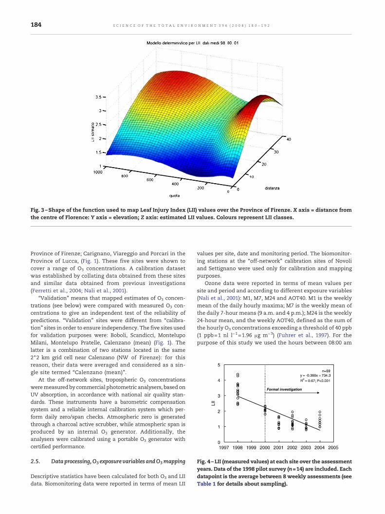
Fig. 3 –Shape of the function used to map Leaf Injury Index (LII) values over the Province of Firenze. X axis = distance fromthe centre of Florence: Y axis = elevation; Z axis: estimated LII values. Colours represent LII classes.
Fig. 4 –LII (measured values) at each site over the assessmentyears. Data of the 1998 pilot survey (n=14) are included. Eachdatapoint is the average between 8 weekly assessments (seeTable 1 for details about sampling).
184 S C I E N C E O F T H E T O T A L E N V I R O N M E N T 3 9 6 ( 2 0 0 8 ) 1 8 0 – 1 9 2
Province of Firenze; Carignano, Viareggio and Porcari in theProvince of Lucca, (Fig. 1). These five sites were shown tocover a range of O3 concentrations. A calibration datasetwas established by collating data obtained from these sitesand similar data obtained from previous investigations(Ferretti et al., 2004; Nali et al., 2001).
“Validation” means that mapped estimates of O3 concen-trations (see below) were compared with measured O3 con-centrations to give an independent test of the reliability ofpredictions. “Validation” sites were different from “calibra-tion” sites in order to ensure independency. The five sites usedfor validation purposes were: Boboli, Scandicci, MontelupoMilani, Montelupo Pratelle, Calenzano (mean) (Fig. 1). Thelatter is a combination of two stations located in the same2 ⁎2 km grid cell near Calenzano (NW of Firenze): for thisreason, their data were averaged and considered as a sin-gle site termed “Calenzano (mean)”.
At the off-network sites, tropospheric O3 concentrationsweremeasured by commercial photometric analysers, basedonUV absorption, in accordance with national air quality stan-dards. These instruments have a barometric compensationsystem and a reliable internal calibration system which per-form daily zero/span checks. Atmospheric zero is generatedthrough a charcoal active scrubber, while atmospheric span isproduced by an internal O3 generator. Additionally, theanalysers were calibrated using a portable O3 generator withcertified performance.
Descriptive statistics have been calculated for both O3 and LIIdata. Biomonitoring data were reported in terms of mean LII
values per site, date and monitoring period. The biomonitor-ing stations at the “off-network” calibration sites of Novoliand Settignano were used only for calibration and mappingpurposes.
Ozone data were reported in terms of mean values persite and period and according to different exposure variables(Nali et al., 2001): M1, M7, M24 and AOT40. M1 is the weeklymean of the daily hourly maxima; M7 is the weekly mean ofthe daily 7-hour means (9 a.m. and 4 p.m.); M24 is the weekly24-hour mean, and the weekly AOT40, defined as the sum ofthe hourly O3 concentrations exceeding a threshold of 40 ppb(1 ppb=1 nl l−1=1.96 μg m−3) (Fuhrer et al., 1997). For thepurpose of this study we used the hours between 08:00 am
Fig. 5 –Spatial distribution of mean estimated LII values over the period 2000–2003. LII classes are reported. The map refers tothe grey area of Fig. 1.
185S C I E N C E O F T H E T O T A L E N V I R O N M E N T 3 9 6 ( 2 0 0 8 ) 1 8 0 – 1 9 2
and 08:00 pm (EC Directive 2002/3), which is slightly differentfrom the hours with global radiation N50 W m−2, recom-mended by the UN/ECE (UN/ECE, 2004).
The relationship between the O3 exposure variables (M1,M7, M24 and AOT40) and LII was investigated by means of
Table 2 – Descriptive statistics ofweeklyM1,M7,M24 andAOT40of Florence over the investigated periods (see Table 1) in the re
Mean of weekly mean vales between different stations and standard dev
non-parametric correlation analysis (Spearman Rank OrderCorrelation). First order linear regressionwas used to derive acalibration function and to predict O3 concentrations. Uncer-tainty in prediction was evaluated by the standard error ofestimates of the regression.
registered at the automaticmonitoring sites in the Provincelevant years
Fig. 6 –Time development of O3 M1 (μg m−3) over the period1996–2004 at the conventional monitoring station of theProvince of Florence (after Ferretti et al., 2004). The regressionrefers only to those site active at all monitoring years (Boboli,Montelupo Milani, Novoli, Settignano).
Fig. 7 –Standardized LII (LIIstd) regressed against O3M1 at thecalibration sites. Calibration sites within the Florence areaare denoted by filled symbols; calibration sites in theProvince of Lucca are denoted by open symbols. A: Individualsurvey years; B: average between years. Error bars on graph Brepresent the standard deviation between the various surveyyears at the same site.
186 S C I E N C E O F T H E T O T A L E N V I R O N M E N T 3 9 6 ( 2 0 0 8 ) 1 8 0 – 1 9 2
Mapping of LII over the study area was carried outaccording to an ad-hoc deterministic model parameterisedon the basis of the data obtained from the pilot study in 1998and the two “formal” surveys in 2000 and 2001. The modelaccounted for the dependence of LII on elevation and distancefrom the centre of Firenze (Ferretti et al., 2004). The modelused was as follows and included two Gaussian components(Fig. 3):
LII d:qð Þ ¼ a21 � exp � d� d1rd1
!2
� q� q1rq1
!224
35
þa22 � exp � d� d2rd2
!2
� q� q2rq2
!224
35
ð3Þ
where:
d and q are distance from the city centre of Firenze andelevation, respectively;a1 and a2 are squared to avoid negative values that wouldinvert the relevant Gaussian component;(d1, q1) and (d2, q2) are the points where the two Gaussiancomponents of the model reach their maximumσ1d, σ2
d, σ1q, σ2
q are the variances of the Gaussian components.
The model was used to estimate LII values for 2 ⁎2 kmgeographical grid cells for each survey year: 2000, 2001, 2002,2003 and 2004. “Average”mapswere produced on the basis of
Table 3 – Correlation and regression analysis between ozone (v
No. of observations, Spearman correlation coefficient, and P-level. Coefficlinear models and standard error of the estimates of the regressions.
all stations that were operational over the period 2000–2003.Data from the year 2004were not used for the “average”mapsbecause the sites in 2004 were the same as in 2000.
2.6. Quality Assurance
QualityAssurance (QA) procedureswere adopted to ensure dataconsistency and comparability in both time and space. For the
ient of determination, P-level, equation coefficients for the first order
187S C I E N C E O F T H E T O T A L E N V I R O N M E N T 3 9 6 ( 2 0 0 8 ) 1 8 0 – 1 9 2
biomonitoring network, they included: adoption of StandardOperating Procedures (SOPs), annual training and inter-calibra-tion between observers, and field checks. Measurement QualityObjective (MQO) was set at ±1 assessment class and DataQuality Limits (DQLs) at 90% of compliance of MQOs (Ferretti etal., unpublished data). Overall, 4350 cross-comparisonsof individual leaf injury assessment were carried out in thetraining sessions of the surveys. MQOs were achieved in mostcases (range: 70–95%), while deviations exceeding two assess-mentclasseswere limited (3–7%). For theair qualitynetwork,QAprocedures included SOPs, daily 0-span, data completenesschecks and seasonal calibration of the O3 analysers.
3. Results
3.1. Leaf injury and ozone levels during the2000–2004 period
Ozone inducedvisible leaf injurywas recordedonaweeklybasisat all sites. There were considerable spatial and temporal var-iations (Figs. 4 and 5). When the data from the 1998 pilot sur-vey were taken into account, a significant decrease in visible LIIvalues was observed (Fig. 4). However, within the formal inves-tigation period, a statistically significant difference was identi-fied between 2000 and the other years (Tukey HSD, HonestSignificance Difference, Pb0.05). This may in part be explainedby the fact that samplingwas carried out from July to Septemberin 2000 as opposed to June to August in the other years (2002–2004) (see Table 1), although differences in plant sensitivitybetween years cannot be ruled out. On average (2000–2003),mapped LII was higher for a broad band surrounding Firenze,from north-east to west. Another area with high visible LII wasobserved to the east of Firenze, corresponding to the Apenninemountains (Fig. 5).
Measured O3 concentrations are presented in Table 2 andFig. 6. Minimum concentrations were recorded at Novoli whilemaximum concentrations were reported for Montelupo Pra-telle. Significant differences occurred between Novoli and theother stations (TukeyHSDafter 1-wayANOVA, P=0.03). Similarto the LII data, a significant decrease was observed when the1998 data were considered (Fig. 6), but no statistically sig-nificant change was recorded over the period 2000–2004. Notethat O3 concentrations from 2003, a year often reported ashaving particularly high O3 concentrations in many parts ofEurope (see EEA, 2003), were only slightly different from theother years in the Firenze area, at least over the survey period.It is worth noting, however, that significant differences be-tween 2003 O3 concentration data and the historical serieswere reported for theperiod4–13August (Pellegrini et al., 2007),a period only partly covered by this project.
M24, M7, M1 and AOT40 calculated from the automaticanalyserswere averaged and comparedwithmeanLII from thesame sites and time period. Table 3 reports the correlationcoefficients between O3 exposure variables and standardizedLII; the same table also reports the coefficients of the re-gression functionswhen LII was used as a proxy indicator of O3
concentration. In addition, Fig. 7 shows a scatterplot of M1 vs.standardized LII based on individual sites and years (a) and ondata averaged at site level over all the investigated years (b).
The scatter in Fig. 7 (a), was considered to result fromanumberof factors including the fact thatO3 effects on plants aremainlydriven by uptake, rather then concentration in the atmosphere(e.g., Reich, 1987; UN/ECE, 2004). Therefore, some variability inresponse can be due to unexpected conditions leading to O3
uptake (Reich, 1987; Klumpp et al., 2006). In addition, factorsrelated to thebiological component of the system (e.g., possiblechanges in plant sensitivity, random factors affecting plants,such as insect, fungal, mechanical damage, which may alsoalter the response to O3), the conventional analyser compo-nent (e.g., measurement errors), and the observers (e.g., clas-sification and measurement error) may also result in somenoise. When data were aggregated (Fig. 7, b), there was con-siderable smoothing of the variation inherent in the systemand an increase in the proportion of variance explained(R2=0.95). Similar results were obtained by Ribas and Peñuelas(2003).
3.2. Estimates of ozone concentration and their reliability
The spatial distribution of the predicted M1 O3 concentrationsare reported for each year of investigation in Fig. 8 at a 2 ⁎2 kmspatial resolution. High O3 concentrations were estimatedoutside the urban area of Firenze, and mainly related to the Nand N–E part of the province, up to the most remote Apennineranges. A second area of high O3 concentrations was south ofFirenze, a hilly area with extensive vineyards. It is worthnoting the completely different pattern in the year 2003, whenhigher O3 concentrations were estimated for the area west ofFirenze. M7, M24 and AOT40 had similar spatial patterns withrespect to M1(data not shown). Table 4 reports the frequencyof grid cells in different classes of M1. The year 2003 was theone with the highest frequency of high values, and the year2004 the year with the lowest.
Given the considerable year to year variation in terms ofspatial pattern, a more robust picture of O3 pollution over agiven region requires several years of monitoring. For exam-ple, the UN/ECE (UN/ECE, 2004) and the EUDirective 2002/3 (EC,2002) recommend a 5-year period is necessary to obtainreliable estimates useful for risk analysis for forest vegetation.Consequently, 2000–2003 data have been processed jointly. Itis worth noting that the 2000–2003 map is based on 53 sites,while annual maps used a maximum of 15 sites. The average(2000 to 2003) M1 map is shown in Fig. 8 (bottom right). Highvalues were estimated in the areas E and NE of Firenze (meanM1 120–160 μg m−3, with peak of 160–200 μg m−3) and in the Sand SW part of the province (120–140 μgm−3). The pattern wassimilar for all O3 exposure variables (data not shown) and wasparticularly important for AOT40, whose estimated values canreach 5000 μg m−3 h per week (ca. 2500 ppbh per week). Thismeans that the critical levels set to protect crops, seminaturalvegetation (6000 μg m−3 h over three months, UN/ECE 2004)and forests (10,000 μg m−3 h over six months, UN/ECE, 2004)may often be exceeded in summer months. These results areof particular interest when considering that the Province ofFirenze includes approximately 1570 km2 of forest, approxi-mately 1530 km2 of crops and 136 km2 of vineyards.
In order to test the reliability of the estimates, the mappedestimates of O3 M1 values for two to five “off-network” val-idation sites were compared to measured values. Overall, the
188 S C I E N C E O F T H E T O T A L E N V I R O N M E N T 3 9 6 ( 2 0 0 8 ) 1 8 0 – 1 9 2
Table 4 – Frequency of 2×2 km grid cells in differentclasses of ozone concentration (M1)
Estimatedozone, M1,μg m−3
Frequency of grid cells, %
2000(n=857)
2001(n=857)
2002(n=857)
2003(n=857)
2004(n=857)
b80 4.67 5.83 4.67 3.15 5.7280 to b100 16.34 13.89 11.67 18.79 8.05100 to b120 34.65 35.35 39.31 38.97 34.54120 to b140 30.22 30.11 31.16 23.80 40.14140 to b160 10.74 13.65 10.15 10.27 11.55160 to b180 3.38 1.17 2.57 4.32 0.00N180 0.00 0.00 0.47 0.70 0.00
189S C I E N C E O F T H E T O T A L E N V I R O N M E N T 3 9 6 ( 2 0 0 8 ) 1 8 0 – 1 9 2
two data series (measured vs. predicted) did not differ sig-nificantly and estimated values were within the range ofmeasured values (Wilcoxon Matched Pairs test, P=0.34). At theindividual site level, in general, the consistency betweenmeasured and estimated values was acceptable (Fig. 9),although considerable differences existed for certain sites andyears. In particular, a substantial, generalized underestimationwas observed for the 1998 pilot dataset. Estimated O3 concen-trations had on average an error of 18% (ranging from 1.6–58%)for M1: this falls within the accepted range of uncertaintyas defined in the EU Directive 2002/3 for modelled valuesand estimates, which have an accepted level of 50 and 75%,respectively.
4. Discussion
The scientific value and importance of the results obtained inthis study can be considered in relation to their practicalapplication for environmental management. From a scientificpoint of view, there are three main elements to be considered:the integration of O3 networks, the reliability of bioindicators,and the value of exposure–response functions.
The integration of originally disparate and independent O3
networks is an issue of concern for managers of monitoringprogrammes who are currently facing reductions in fundingcoupled with increasing reporting obligations (Olsen et al., 1999).When networks to be integratedwere originally designed using astatistical (probabilistic) approach, the integration is possible,although difficult. Unfortunately, air quality and biomonitoringnetworks have not traditionally been established following aprobabilistic sampling design and therefore statistical inferenceand/or integration is a challenging task. In our investigation,while the biomonitoring network was designed on the basis of asampling design, the existing network of conventional O3 mon-itors was based on a purposive selection of sites. Consequently,the only option for integration was to locate some “off-network”biomonitoring sites on the same sites as the conventional O3
monitors, derive a calibration function, anduse sucha function topredict the value of the variable of concern (O3 concentration) atthe “in-network” biomonitoring sites (see Overton et al., 1993). Inthis respect, the importance of adopting formal statistical designprinciples in biomonitoring should be emphasised (e.g. Ferrettiand Erhardt, 2002). When large-scale networks are concerned,however, some question may arise regarding their feasibility inrelation to the considerable logistic effort required. Althoughexamples of feasibility exists (see Klumpp et al., 2006), optionssuch as the US Forest Service bioindicator programme andthe European ICP-Forests O3 symptoms survey (Bussotti et al.,2006; Smithet al., 2003) canbeof value, especially in remoteareas.These approaches are based on sensitive native species at thesites, and thishasconsiderableadvantages froma logisticpointofview. However, the use of native, non-standard bioindicatorsimplies considerable noise due to different intra- ad inter-speciessensitivity.
Fig. 8 –Predicted mean M1 values (μg m−3) for the 8-week per5 June – 31 July 2002; 12 June – 7 August 2003; and 9 June – 4 Asampling sites. The maps refer to the grey area of Fig. 1.
Reliability of data from tobacco plant were discussed byLorenzini et al. (2000) in terms of observer error (thatmay affectthe comparability of results through time and space), and byVergé et al. (2002) in terms of intra-population variability andnon-linearityof response (thatmayaffect the comparability andthevalue of linearmodels to predict leaf injuryon the basis ofO3
concentrations). In the former case, a reliableQuality Assuranceprogramme has been shown to be essential to control observererror, and our results support this view. In the latter case, intra-population variability certainly exists, but the effects on thesurvey results might be minimal if population individuals wereallocated at monitoring stations on a random basis.
The value of the exposure–response function has beenpreviously reported by Krupa et al. (1993). In their study, basedon the analysis of exposure–response functions obtained fromopen-top chamber experiments, they stated that “visible foliarresponse of tobacco Bel W3 can be used as a qualitative, but notnecessarily as a quantitative indicator of relative ambient O3 on ageneralized temporal or spatial scale”. In a more recent study,Ribas and Peñuelas (2003) pointed out the importance of soil andatmospheric factors (e.g., Vapour Pressure Deficit) in controllingfoliar O3 uptake (that may affect the nature of the exposure–response functions). However, they concluded that, despitecertain limitations, “it was possible to make quantitativeinferences about air quality for O3 on the basis of plant symptomexpression alone, at least at the annual and regional scales”.According to the results of thepresent investigation, bothauthorsare right in the sense that exposure–response functionscannotbegeneralized, but must be developed for each investigation, andmust always be evaluated against independent measurements.Regular watering of plants is also essential to control soil andatmospheric humidity. In our project, the planned use ofcalibration sites allow tailored calibration functions, and regularwatering allowed the performance of the plants to bemaintainedat an optimum, thus reducing the influence of themodifiers of O3
uptake. Also, aggregating data on a temporal basis helped reducethe effects of random natural factors.
From a practical point of view, it is worth noting that, inEurope, national to regional administrations are mandated fromthe European Union to identify and classify those areas where O3
concentrations are expected to exceed the target and the long-
iods: 17 July–11 September 2000; 13 June – 8 August 2001;ugust 2004. Grid cells are 2×2 km. Crosses represent the
190 S C I E N C E O F T H E T O T A L E N V I R O N M E N T 3 9 6 ( 2 0 0 8 ) 1 8 0 – 1 9 2
termobjectives set by the EU 2002/3Directive. Given the nature ofground level O3 (it persists in high levels particularly in rural andremote areas), it is unlikely that this classification can be done onthe basis of the traditional O3 analysers which aremostly locatedin urban areas: Fig. 1 clearly demonstrates the uneven spatialcoverage of the Firenze area by the conventional O3 monitors.Large-scale models (e.g. EMEP, Simpson et al., 2003) are dataintensive andmay not functionwell at local scales, while the useof models such as CALGRID (Yamartino et al., 1992) that can berunat a local level, require considerable investmentandexpertiseas well as also being data intensive. In both cases, independentvalidation is required. While some effort is currently beingmadeto install aminimum set of background automatic O3monitoringstations, it is unlikely that this will allow a satisfactory spatial
Fig. 9 –Measured and predicted ozone M1 concentrations at theMeasured valueswere actuallymeasured using conventional O3
cell where the conventionalmonitor is located. Error bars indicatvalues are one per year, no standard deviation is reported for trefers to the pilot study undertaken before the formal survey 2
coverage. In this respect, together with (e.g.) passive sampling(Sanz et al., 2007), biomonitoring represents a valid and reliablesolution to supplement physical–chemical O3 monitors, espe-ciallywhennot only the concentrations, but also the impact of O3
on living organisms is of concern.
5. Conclusions
A pre-existing network of conventional O3 analysers togetherwith a newly designed biomonitoring network containing thesupersensitive tobacco Bel W3 plants was integrated into onescheme in order to obtain estimates of O3 concentrations over
“off-network” validation sites in different years (see Fig. 1).monitors. Predicted values are estimates for the 2×2 km gride the standard deviation ofmeasured values. Since predictedhe prediction at individual sites. The data for the year 1998000–2004 and recalculated afterwards.
191S C I E N C E O F T H E T O T A L E N V I R O N M E N T 3 9 6 ( 2 0 0 8 ) 1 8 0 – 1 9 2
a 3513 km2 area, around Firenze, Tuscany, Italy. Leaf InjuryIndex (LII) on tobacco plants was significantly related to O3
exposure (P values between 0.018 and 0.0014) as expected andwas used to predict atmospheric O3 concentrations (P valuesbetween 0.0048 and 0.0009). Estimated O3 concentrations overthe study area exhibited an average error of 18% (ranging from1.6–58%) for the M1. The study provided evidence that in-tegration of monitoring networks using different methods,with different set-up mechanisms and costs can be a viableoption when acceptable (e.g., statistically significant, withknown precision) estimates of O3 concentrations over largeareas is of concern. In our application, bioindicators wereused to supplement physical–chemical monitoring systems,but in principle this applies also to different, low-cost mea-surement techniques (e.g. passive sampling). In future appli-cations, our mapped estimates will render it possible toidentify and quantify areas where human health and vegeta-tion can be at potential risk from O3 according to the currentregulations, knowledge, protection limits and uncertaintylevel. This information is essential formonitoring the progressin achieving the target of reducing areas where O3 concentra-tions exceed critical concentrations.
Acknowledgements
A number of people from the Provincia di Firenze, the regionalenvironmental protection agency (ARPAT) and commoncitizens that cannot be mentioned here contributed to thisproject. We acknowledge in particular Enrico Cenni, AlbertoCozzi, Renzo Nibbi and Cinzia Sarti (Linnaeambiente RicercaApplicata), involved in setting-up the system, designing thebiomonitoring stations and carrying out the field checks.Federico Lazzaroni produced Figs. 1, 5 and 8 and assisted at theearly stages of the monitoring design. We are also grateful toDr. Alison Donnelly (Trinity College, Dublin) for the linguisticrevision and stimulating comments.
R E F E R E N C E S
Brunekreef B, Holgate ST. Air pollution and health. Lancet2002;360:1233–42.
Bussotti F, Cozzi A, Ferretti M. Field surveys of ozone symptomson spontaneous vegetation. Limitations and potentialities ofthe European programme. Environ Monit Assess2006;115:335–48.
Eberhardt LL, Thomas JM. Designing environmental field studies.Ecol Monogr 1991;61:53–73.
EEA—European Environment Agency. Air pollution by ozone inEurope in summer 2004. Copenhagen: European EnvironmentAgency; 2005. 34 pp.
EEA—European Environment Agency. Air pollution by ozone inEurope in summer 2003. Summary report. Copenhagen:European Environment Agency; 2003. 5 ps.
EC—European Commission. Directive 2002/3/EC of the EuropeanParliament and of the Council of 12 February 2002 relating toozone in ambient air, vol. 067. Official Journal L; 2002. p. 0014–30.09/03/2002.
Felzer BS, Reilly JM, Melillo JM, Kicklighter DW, Wang C, Prinn RG,et al. Past and future effects of O3 on net primary productionand C sequestration using a global biogeochemical model. MITjoint programme on the science and policy of global change,vol. 103. Report; 2004.
Ferretti M, Erhardt W. Key issues in designing biomonitoringprogrammes. Monitoring scenarios, sampling strategies andquality assurance. In: Nimis PL, Scheidegger C, Wolseley PA,editors. Monitoring with lichens — monitoring lichens. KluwerAcademic Publisher; 2002. p. 111–39.
FerrettiM,Cenni E, PisaniB,Righini F,GambicortiD,DeSantisP, etal.Biomonitoraggio di inquinanti atmosferici - un'esperienzaintegrata nella Toscana costiera. Acqua Aria 1992;8:747–58.
Ferretti, M., Mansuino, S., Pallicca, P. Progetto pilota europeo sull'usodi bioindicatori di inquinamento atmosferico in aree urbane -Manuale di Campagna, unpublished data. Unpublished, forinternal use. Available by [email protected].
Ferretti, M., Andrei, S., Caldini, G., Galanti, E., Grechi, D. Il SistemaPermanente Integrato per il Monitoraggio della Qualitàdell'Aria nella Provincia di Firenze (SPIMQA). Sintesi deirisultati 2000–2004. Progetto “Qualità dell'aria nella provincia diFirenze valutata mediante monitoraggio biologico.” Projectpackage 1. Report to the Provincia di Firenze, Direzione TutelaAmbiente, 2004; 37 pp.
Fowler D, Cape N, Coyle, Flechard C, Kuylenstierna J, Hicks K, et al.The global exposure of forest ecosystems to air pollutants.Water Air Soil Pollut 1999;116:5–32.
Fuhrer J, Skärbi L, Ashmore MR. Critical levels for ozone effects onvegetation in Europe. Environ Pollut 1997;97:91–106.
Heggestad HE. Origin of Bel-W3, Bel-C and Bel-B tobacco varietiesand their use as indicator of ozone. Environ Pollut1991;74:264–91.
IPCC. Climate change 2007: the physical science basis. Summaryfor policymakers. Contribution of working group I to the fourthassessment report of the intergovernmental panel on climatechange. IPCC Secretariat, Geneva (CH); 2007. ND: 21 ps.
Klumpp A, AnselaW, Klumpp G, Vergne P, Sifakis N, Sanz MJ, et al.Ozone pollution and ozone biomonitoring in European citiespart II. Ozone-induced plant injury and its relationship withdescriptors of ozone pollution. Atmos Environ 2006;40(38):7437–48.
Krupa SV, Manning WJ, Nosal M. Use of tobacco cultivars asbiological indicators of ambient ozone pollution: an analysis ofexposure–response relationships. Environ Pollut 1993.
Lorenzini G. Piante vascolari come bioindicatori della qualitàdell'aria (inquinamento da ozono): proposte metodologiche.In: Piccini C, Salvati S, editors. Atti del WorkshopBiomonitoraggio della qualità dell'aria sul territorionazionale. Serie: Atti 2/1999, Agenzia Nazionale per laProtezione dell'Ambiente; 1999. p. 199–216.
Lorenzini G, Guidi L, Panattoni A. Valutazione dei livelli e deglieffetti di inquinanti atmosferici con l'impiego di indicatoribiologici. Risultati di un'esperienza su scala regionale. AcquaAria 1988;3:289–302.
Lorenzini G, Nali C, Biagioni M. Long-range transport ofphotochemical ozone over the Tyrrhenian Sea demonstratedby a new miniaturized bioassay with ozone-sensitive tobaccoseedlings. Sci Total Environ 1995;166(1–3):193–9.
Lorenzini G, Nali C, Dota MR, Martorana F. Visual assessment offoliar injury induced by ozone on indicator tobacco plants: adata quality evaluation. Environ Monit Assess 2000;62:175–91.
Manning WJ, Feder W. Biomonitoring air pollutants with plants.Barking: Applied Science Publishers; 1980. 142 pp.
Nali C, Ferretti M, Pellegrini M, Lorenzini G. Monitoring andbiomonitoring of surface ozone in Firenze, Italy. Environ MonitAssess 2001;69(2):159–74.
Nali C, Pucciariello C, Lorenzini G. Mapping ozone critical levels forvegetation in Central Italy. Water Air Soil Pollut 2002a;141(1–4):337–47.
192 S C I E N C E O F T H E T O T A L E N V I R O N M E N T 3 9 6 ( 2 0 0 8 ) 1 8 0 – 1 9 2
Nali C, Pucciariello C, Lorenzini G. Ozone distribution in centralItaly and its effect on crop productivity. Agric Ecosyst Environ2002b;90(3):277–89.
Olsen AR, Sedrransk J, Edwards D, Gotway CA, Ligget W, RathbunS, et al. Statistical issues for monitoring ecological and naturalresources in the United States. Environ Monit Assess1999;54:1–45.
Overton JMcC, Young TC, Overton WS. Using “found” data toaugment a probability sample: procedure and case study.Environ Monit Assess 1993;26:65–83.
Pellegrini W, Lorenzini G, Nali C. The 2003 European heat wave:which role for ozone? Some data from Tuscany, Central Italy.Water Air Soil Pollut 2007;181:401–8.
Regione Toscana Giunta Regionale. Direzione Generale PoliticheTerritoriali e Ambientali, area Qualità dell'aria, rischiindustriali, prevenzione e riduzione integratadell'inquinamento, – Valutazione della qualità dell'ariaambiente nel periodo 2000–2002 e classificazione del territorioregionale ai sensi degli articoli 6, 7, 8 e 9 del Decreto Legislativon. 351/99. Firenze: EDIFIR; 2004. 94 pp.
Reich PB. Quantifying plant response to ozone: a unifying theory.Tree Physiol 1987;3:63–91.
Ribas A, Peñuelas J. Biomonitoring of tropospheric ozonephytotoxicity in rural Catalonia. Atmos Environ 2003;37:63–71.
Sanz MJ, Calatayud V, Sanchez-Peña G. Ozone concentrationsmeasured by passive sampling at the Intensive MonitoringPlots of South Western Europe. Environ Pollut 2007;145:620–8.
Saitanis CJ. Background ozone monitoring and phytodetection inthe greater rural area of Corinth—Greece. Chemosphere2003;51:913–23.
Simpson D, Fagerli H, Jonson JE, Tsyro S, Wind P. Transboundaryacidification, eutrophication and ground level ozone in Europe.Part I — unified EMEP model description. Oslo: Norwegian
Meteorological Institute; 2003. p. 104. EMEPMSC-WNote 1/2003,(http://www.emep.int/publ/common_publications.html).
Smith G, Coulston J, Jepsen E, Prichard T. A national biomonitoringprogram — results from field surveys of ozone sensitive plantsin northeastern forests (1994–2000). Environ Monit Assess2003;87:271–91.
Steubing L, Jäger HJ. Monitoring of air pollutants byplants — methods and problems. Proceed. Internationalworkshop, Osnabrück 24–25, 1981. The Hague, The Netherlands:Dr. W. Junk Publishers; 1982.
Stevens D. Implementation of a national monitoring program.J Environ Manag 1994;42:1–29.
UN/ECE. Mapping Manual Revision 2004. UNECE Convention onLong-range Transboundary Air Pollution. Manual on themethodologies and criteria for modelling and mapping criticalloads and levels and air pollution effects, risks and trends.2004. www.icpmapping.org.
Van Meirvenne, M. Characterization of soil spatial variation usinggeostatistics. Rijksuniversiteit Gent, Fakultet van deLandbouwwetenschappen, Laboratorium voor AgrarischeBodenkunde, Ph. D. Thesis, 1991: 45 pp.
Vergé X, Chapuis A, Delpoux M. Bioindicator reliability: theexample of BelW3 tobacco (Nicotiana tabacum L.). Environ Pollut2002;118:337–49.
Vingarzan R. A review of surface ozone background levels andtrends. Atmos Environ 2004;38:3431–42.
Volz A, Kley D. Evaluation of the Montsouris series of ozonemeasurements made in the nineteenth century. Nature1988;332:240–2.
Yamartino RJ, Scire JS, Carmichael GR, Chang YS. The CALGRIDmesoscale photochemical grid model — I. Model formulation.Atmos Environ 1992;26A:1493–512.